Distributed robust secondary frequency control of inverter-based microgrids under time-varying communication delays

Abstract

This paper presents a robust secondary control strategy for frequency synchronization and active power sharing for inverter-based microgrids. The problem is addressed in a multi-agent fashion where the local controllers of the distributed generators play the role of agents, and communication is affected by time-varying delays. The approach is fully distributed and based on a synergic combination of linear consensus and integral sliding-mode control. Lyapunov analysis is presented to assess the stability properties of the closed loop. Delay-dependent stability conditions are expressed as a set of linear matrix inequalities whose solution yields appropriate control gains such that frequency restoration is achieved despite delays and active power sharing constraints. Simulations confirm the effectiveness of the proposed control strategy.

I Introduction

Microgrids (MGs) are small-scale power grids consisting of localized grouping of heterogeneous renewable Distributed Generators (DGs), storage systems, and loads. MGs operate either in islanded, autonomous mode or connected to the main power grid. The control of an AC MG has been recently standardized into a three-layered, nested, control architecture [1]. This structure includes a local Primary Control (PC) level (droop control and primary stabilization), a centralized or distributed Secondary Control (SC) level (voltage and frequency restoration), and a tertiary control level (optimal operation). Among the three, the frequency SC task is of more practical interest to make the integration of renewable generation compliant in the existing fixed-frequency power transmission paradigm. It is also worth mentioning that temporarily modifying the MG frequency while preserving the power sharing among DGs is also useful to perform seamless transition of the MG from islanded to grid-connected mode [2].
Early SCs were centralized [1]. These solutions are now discouraged in favour of distributed approaches because they scale better with the MG size, are more robust to failures, and dispense from costly central computing and communication units [3]. Pioneering work that solves the frequency SC problem in a distributed fashion is reported in [4]. There, a distributed averaging proportional integral scheme is proposed, and power compensation terms are aimed to meet the desired power sharing among DGs. In contrast with [4], where the SC set-points are assumed known to all the DGs, later leader-follower strategies have been proposed. These allow for arbitrary adjusting of the MG frequency in a distributed way by acting on the leader DG only. As an example, [5] proposes a leader-based interaction rule and proves its stability features in the local sense.
Although the mentioned strategies require a communication infrastructure, network-induced communication delays, which may degrade the MG performance and even destabilize it, have seldom been considered. The impact on SC of a constant identical delay for all communication links is analyzed in [6] and [7]. An SC that accounts for time-varying delay is considered in [8]. A distributed finite-time control protocol for frequency and voltage restoration under a unique constant delay affecting the communication network is proposed in [9], whereas [10] only addresses the finite-time voltage control problem. Along this line, recent works [11, 12, 13] suggest event-triggered SC approaches with time-varying communication delays. Although all works mentioned above are promising, they all rely on perfect knowledge of the DG mathematical models and power measurements.
Thus motivated, this paper proposes a leader-oriented frequency SC strategy capable of restoring DG frequencies to the desired value and establishing active power sharing accuracy in spite of delays in the communication between DGs and unknown load variations. We design a distributed SC consensus protocol consisting of two distinct terms: a nonlinear sliding-mode-based discontinuous term and a linear time-delay consensus protocol. The nonlinear part of the proposed scheme is an Integral Sliding Mode (ISM)-based discontinuous term using only local measurements, which is employed to suppress the effect of disturbances on the MG emerging behavior. The second term aims to compensate for the unavoidable deviations of the DG output frequencies from the set-point value while preserving the power sharing accuracy condition. In comparison with [6, 7, 8, 11, 12, 13, 9], the proposed strategy requires neither power measurements nor the use of globally known frequency set-points, thus allowing for SC design independently from the PC loop (i.e., the frequency restoration approach presented in this work is inherently robust against load variations). As opposed to [10], the frequency restoration problem and achieving active power-sharing are the focus of this paper. The main contributions of the present work are as follows: (i) We demonstrate that in the absence of disturbance terms affecting the MG, the linear time-delay consensus protocol forces the output frequency of each DG to synchronize with the set-point value despite time-varying communication delays. (ii) We prove that considering the presence of the disturbance terms yields after a finite transient a sliding motion along which the MG exhibits the same trajectories of the disturbance-free linear dynamics under the linear time delay consensus protocol, for which the achievement of frequency restoration and active power sharing accuracy was previously demonstrated. (iii) By employing a Lyapunov-Krasovskii function, we derive a delay-dependent control gain tuning procedure, represented as a set of Linear Matrix Inequalities (LMIs) whose solution allows for finding the appropriate control gains. (iv) Lastly, it is worth mentioning that although the proposed SC has some discontinuous control components since they appear only in their time derivatives, the actual control inputs are smooth. Therefore, they can safely be used to feed the inner PCs [1]. Preliminary results of this research, limited to the voltage SC design, have been presented in [14].

The article is structured as follows: some preliminary notions and notations are recalled in Section II. Section III provides the nonlinear inverter-based MG model for SC purposes. The frequency SC problem, along with the proposed strategy and the main results are illustrated in Section V. Computer simulations are discussed in Section VI. Finally, Section VII provides concluding remarks.

II Mathematical Preliminaries and Notations

Notation: The complex, real, and positive numbers sets are denoted by $\mathbb{C}$, $\mathbb{R}$, and $\mathbb{R}^{+}$, and $\imath=\sqrt{-1}$. Let $A=[A_{ij}]\in\mathbb{R}^{n\times n}$, its transpose is $A^{\intercal}$. Assume $A$ symmetric, $A\succ 0$ ($A\succeq 0$) denotes $A$ positive (semi-) definite. $I_{n}$ is the $n$-dimensional identity matrix and $1_{N}$ is a vector with all $N$ elements equal to 1. $\mathrm{card}(\mathcal{X})$ is the cardinality of set $\mathcal{X}$. Finally, the $\text{SIGN}(\cdot)$ operator denotes the discontinuous multi-valued function

$$\text{SIGN}(\mathcal{S}_{i}(t))\in\begin{cases}1&\text{if }\mathcal{S}_{i}(t)>0\\ [1,-1]&\text{if }\mathcal{S}_{i}(t)=0\\ -1&\text{if }\mathcal{S}_{i}(t)<0\end{cases}$$

Graph Theory: A graph $\mathcal{G}_{N}(\mathcal{V},\mathcal{E})$ is a topological tool used to describe pairwise interactions between nodes, or agents in the multi-agent field. The node set is $\mathcal{V}=\{1,2,\ldots,N\}$, whereas the edge set $\mathcal{E}\subseteq\{\mathcal{V}\times\mathcal{V}\}$ describes the pairwise interactions between nodes. The adjacency matrix of $\mathcal{G}_{N}$ is $\mathcal{A}=[\alpha_{ij}]\in\mathbb{C}^{N\times N}$, and $\alpha_{ij}$ denotes the edge’s weight. If $(i,j)\notin\mathcal{E}$ then $\alpha_{ij}=0$, otherwise $\alpha_{ij}\neq 0$. A directed path is an alternating sequence of nodes and edges with both endpoints of an edge appearing adjacent to it in the sequence. Node $i$ is a root node if it can be reached from any other vertex by traversing a directed path.

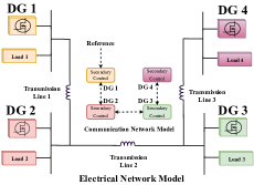
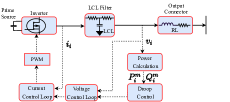
Figure 1: (Left) Cyber and physical layers of a MG composed of four DGs and loads; (Right) Block diagram of the PC.

III Microgrid modeling for SC design

A MG is a cyber-physical system with deeply intertwined components. Interactions among DGs at the cyber and electrical layers can thus be encoded using Graph Theory (see Fig. 1-Left). A DG includes a DC source, a DC/AC inverter, a smoothing filter, a bus connector, and the PC, which embeds current, voltage, and droop control (see Fig. 1-Right). Its aim is to enforce MG stability under the desired power sharing among DGs. By applying the separation principle, the inner current and voltage PC loops can be neglected [15], thus yielding the following simplified DG model [5]

$${\dot{\delta}_{i}(t)=} {~{}\omega_{i}(t)=\bar{\omega}_{i}(t)-k_{P_{i}}P_{i}(t)},\quad\forall i\in\mathcal{V}$$ (1)

$${k_{v_{i}}\dot{v}_{i}(t)=} {-v_{i}(t)+\bar{v}_{i}(t)-k_{Q_{i}}Q_{i}(t)},$$ (2)

where $\delta_{i}$ is the $i$-th DG voltage’s phase angle, $\omega_{i}$ its frequency in rad/sec, and $v_{i}$ its magnitude in $\mathrm{V_{rms}}$. The frequency and voltage SC inputs are $\bar{\omega}_{i}$ and $\bar{v}_{i}$, respectively, $k_{v_{i}}>0$ is the voltage gain, and $k_{P_{i}}$ and $k_{Q_{i}}>0$ are the so-called droop coefficients selected to meet the given real and reactive power sharing specifications. $P_{i}(t)$ and $Q_{i}(t)$ represent active and reactive powers at the DG output ports, dependent on power transmission lines ($P_{ij}$ and $Q_{ij}$) and absorbed powers ( $P_{i}^{L}$ and $Q_{i}^{L}$) at load $i$. For more details on the active and reactive power equations, we refer to [14]. The electrical interaction among DGs over the MG can be encoded by a complex-weighted connected graph $\mathcal{G}^{e}(\mathcal{V},\mathcal{E}^{e})$ being $\mathcal{V}$ the DG set, $\mathcal{E}^{e}$ the power lines, and $\mathcal{A}^{e}=[G_{ij}+\imath B_{ij}]\in\mathbb{C}^{N\times N}$ the complex adjacency matrix, where $G_{ij}$ and $B_{ij}$ denote the conductance and the inductive dominant susceptance between two DGs, respectively. If no connection between the $i$-th DG and the $k$-th DG exists, then $G_{ik}=B_{ik}=0$. Let $\mathcal{N}_{i}^{e}=\{k:k\in\mathcal{V},k\neq i,B_{ik}\neq 0\}$. Finally, it is worth mentioning that if the SC is inactive, then $\bar{\omega}_{i}$ and $\bar{v}_{i}$ in (1)-(2) correspond to the nominal MG utility frequency and rated voltage, e.g., $2\pi 50\mathrm{Hz}$ and $220\mathrm{V_{rms}}$. In the sequel, the following reasonable assumption is made:
Assumption 1 The actual real and reactive power flows at the DG’s output-ports in (1)-(2) are assumed bounded-in-magnitude by a-priori known constants as $|P_{i}(t)|\leq\Pi^{P}_{i}~{},|Q_{i}(t)|\leq\Pi^{Q}_{i},~{}\forall~{}i\in\mathcal{V}.$
Remark 1 Assumption 1 is justified because the power flowing in the lines and/or absorbed by the load is bounded everywhere due to: a) the passive behaviour of loads and lines; b) the bounded operating range of the DC-AC power-converters due to their physical limits; c) the presence of protection apparatus and inner voltage and current PC. This keeps the power flows within pre-specified ranges as discussed, e.g., in [15] and [16].
Define $d_{i}(t)$ as the right-hand side of (1) without the control term, i.e., $d_{i}(t)=-k_{P_{i}}{P}_{i}(t)$. Given Assumption 1 and the stability ensured by the PC, the following holds

$$\exists~{}\Pi\in\mathbb{R}^{+}~{}~{}:~{}~{}|\dot{d}_{i}(t)|\leq\Pi,\quad\forall~{}t\geq 0.$$ (3)

Thus Eq. (1) can be expressed in the next augmented form

$$\dot{\omega}_{i}(t)= \dot{\bar{\omega}}_{i}(t)+\dot{d}_{i}(t)\quad\text{with}\quad\dot{d}_{i}(t)=-k_{P_{i}}\dot{P}_{i}(t)$$ (4)

where $\dot{\bar{\omega}}_{i}$ is the actual control that needs to be designed, and $\dot{d}_{i}$ plays the rule of a time-varying disturbance term.
Remark 2 It is worth remarking that the upper bound (3) on signals $\dot{d}_{i}(t)$ can easily be estimated by means of a terminal sliding-mode disturbance observer implemented within each local controller, see, e.g., [17] and [18].
Cyber MG model: To achieve the SC objectives in a distributed way, DGs are assumed to be provided with computing and communication facilities embedded within their controllers, which play the role of agents. Agents communicate over a network whose topology is encoded by a real-weighted graph $\mathcal{G}^{c}(\mathcal{V},\mathcal{E}^{c})$, where $\mathcal{V}$ is the same node set used to model electrical network $\mathcal{G}^{e}(\mathcal{V},\mathcal{E}^{e})$, whereas $\mathcal{E}^{c}$ is the set of the available communication links. The set of communication neighbors of the $i$-th DG is $\mathcal{N}_{i}^{c}=\{j\in\mathcal{V}:~{}(i,j)\in\mathcal{E}^{c}\}$. According to the leader-follower paradigm, we further assume the existence of a root node, labeled by $0$ in the augmented graph $\mathbb{G}_{N}^{c}(\{0\}\cup\mathcal{V},\mathbb{E}^{c}_{N})$, aimed to provide the SC set-points to a non-empty set of DGs. Clearly, $\mathrm{card}(\mathbb{E}^{c}_{N})>\mathrm{card}(\mathcal{E}^{c})$. Lastly, the set of communication neighbors of the $i$-th DG with respect to graph $\mathbb{G}_{N}^{c}$ is denoted as $\mathbb{N}_{i}^{c}=\{j\in\mathcal{V}:~{}(i,j)\in\mathbb{E}^{c}_{N}\}$.

IV Frequency restoration control problem

Let the desired frequency set-point from the virtual node $0$ be $\omega_{0}>0$. In the absence of SCs, with $\bar{\omega}_{i}=\omega_{0}$ according to (1), the steady-state ($ss$) equilibrium results in $\omega_{i}(\infty)=\omega_{ss}<\omega_{0}$, necessitating frequency restoration. As discussed in [4] and [5] the synchronization condition depends on droop coefficients and the real power balance as

$$\omega_{ss}=\omega_{i}(\infty)=\omega_{0}-\frac{\sum_{k=1}^{N}P_{k}(\infty)}{\sum_{k=1}^{N}\frac{1}{k_{P_{k}}}}\quad\forall~{}i\in\mathcal{V}$$ (5)

and preserves the so-called power-sharing PC objective

$$k_{P_{i}}{P_{i}(\infty)}=k_{P_{k}}P_{k}(\infty)\quad\forall~{}i,~{}k\in\mathcal{V},$$ (6)

whose aim is to enforce a well-defined ratio between the DG injected real power flows. Consider now (1), clearly the achievement of frequency restoration

$$\omega_{ss}=\omega_{i}(\infty)=\omega_{0}\quad\forall~{}i\in\mathcal{V},$$ (7)

under the constraint (6) implies that the frequency SC inputs should be equal to each other at the steady state

$$\bar{\omega}_{i}(\infty)=\bar{\omega}_{ss}\quad\forall~{}i\in\mathcal{V}$$ (8)

being $\bar{\omega}_{ss}$ the frequency SC input at the steady state.

V Frequency secondary control design

To solve the SC problem in a distributed setting with network-induced communication delays, we consider a two-component local interaction protocol as follows

$$\dot{\bar{\omega}}_{i}(t)=\dot{u}^{c}_{i}(t)+\dot{u}^{d}_{i}(t).$$ (9)

The first component $\dot{u}^{c}_{i}(t)$ satisfies the linear consensus protocol dynamics

$$\begin{array}[]{rl}\dot{u}^{c}_{i}(t)=&-\sum_{j\in\mathbb{N}_{i}^{c}}k_{ij}\left(\omega_{i}(t-\tau(t))-\omega_{j}(t-\tau(t)))\right.\\ &-\sum_{j\in\mathcal{N}_{i}^{c}}\overline{k}_{ij}\left(u^{c}_{i}(t-\tau(t))-u^{c}_{j}(t-\tau(t))\right)\end{array}$$ (10)

where ${k_{ij}}$ and $\overline{k}_{ij}$ are scalar control gains to be designed, such that if $(i,j)\in\mathbb{E}^{c}_{N}$ then ${k_{ij}}>0$ and $\overline{k}_{ij}>0$, otherwise ${k_{ij}}=0$ and $\overline{k}_{ij}=0$. $\tau(t)$ is a uniform time-varying delay associated with communication channels. The common assumption of rate-bounded time-varying delays is made [7], [10], and [19].
Assumption 2 Let known bounds $\tau^{\star}$, $\tau_{g}$, exist, such that

$$0\leq\tau(t)\leq\tau^{\star},\quad|\dot{\tau}(t)|\leq\tau_{g}.$$ (11)

To correlate the data received from a DG for feedback purposes, we further assume that:
Assumption 3 $\tau(t)$ is measurable for all $t\geq 0$.
Remark 3 Communication protocols usually include a data-packet time-stamp. Thus, the requirement for detectable delays is costless. Once the delay $\tau(t)$ is detected, by means of local buffers, each controller is enabled to retrieve its own state at that time $t-\tau(t)$, and performs (10). This assumption is common in networked applications, see, e.g., [20] and [7].
The second control component $\dot{u}_{i}^{d}(t)$ in (9) is the discontinuous nonlinear control

$$\dot{u}_{i}^{d}(t)=-m_{i}\;\text{SIGN}(\mathcal{S}_{i}(t)),$$ (12)

where $m_{i}$ are scalar control gains and the sliding variable is defined as $\mathcal{S}_{i}(t)=\omega_{i}(t)-z_{i}(t)$ where $z_{i}(t)$ satisfies

$$\dot{z}_{i}(t)=\dot{u}_{i}^{c}(t),\quad z_{i}({0})=\omega_{i}(0).$$ (13)

Theorem 1 Consider the MG dynamics (1)-(2) under Assumptions 1-3 along with the local interaction rule (9)-(13). Let the gain parameters $m_{i}$ be chosen such that

$$m_{i}>\Pi.$$ (14)

Then, the trajectories of the closed-loop system converge to those of the linear disturbance-free MG dynamics

$$\dot{\omega}_{i}(t)= \dot{u}^{c}_{i}(t)$$ (15)

Proof of Theorem 1. Consider the Lyapunov function

$$\begin{array}[]{rl}V_{i}(t)=&\frac{1}{2}\mathcal{S}_{i}(t)^{2}.\end{array}$$ (16)

By straightforward manipulations, we obtain that along the trajectories of (4), (9)-(13) the time derivative of the sliding variable $\mathcal{S}_{i}(t)$ is given by

$$\begin{array}[]{ll}\dot{\mathcal{S}}_{i}(t)&=\dot{\omega}_{i}(t)-\dot{z}_{i}(t)=\dot{d}_{i}(t)+\dot{u}_{i}^{d}(t)\\ &=\dot{d}_{i}(t)-m_{i}\text{SIGN}(\mathcal{S}_{i}(t)).\end{array}$$ (17)

Hence,

$$\begin{array}[]{rl}\dot{V}_{i}(t)=&\mathcal{S}_{i}(t)\cdot\dot{\mathcal{S}}_{i}(t)=\mathcal{S}_{i}(t)\cdot\dot{d}_{i}(t)-m_{i}\cdot|\mathcal{S}_{i}(t)|.\end{array}$$ (18)

Therefore, by (3) and (14)

$$\begin{array}[]{rl}\dot{V}_{i}(t)\leq&-|\mathcal{S}_{i}(t)|\cdot(m_{i}-\Pi)<0.\end{array}$$ (19)

Then by (13), $V_{i}(0)=0$, which along with (19) yields that

$$V_{i}(t)=0,\quad\forall t\geq 0\quad\rightarrow\quad\mathcal{S}_{i}(t)=0,\quad\forall t\geq 0,$$ (20)

i.e. a sliding motion along the manifold $\mathcal{S}_{i}(t)=0$ takes place from the initial time on. According to the equivalent control method for analyzing the sliding-mode dynamics [21], the trajectories of the discontinuous closed-loop system can be achieved by solving the equivalent closed-loop system where the discontinuous control term $\dot{u}_{i}^{d}(t)$ is substituted by the associated equivalent control $\dot{u}_{i,eq}^{d}(t)$. The latter is computed by solving the equation $\dot{\mathcal{S}}_{i}=0$. It follows from (17) that

$$\dot{u}_{i,eq}^{d}(t)=-\dot{d}_{i}(t),$$ (21)

Replacing (21) for $\dot{u}_{i}^{d}(t)$ in the discontinuous closed-loop dynamics (4), (9)-(13), we can get the disturbance-free MG dynamics (15). $\square$
The point now is to design $\dot{u}_{i}^{c}(t)$ in (15) to achieve the control objectives (7) and (8) asymptotically. Up to now, we found that (9) degenerates into (15) for all $t\geq 0$ according to Theorem 1. It follows that the achievement (7) and (8) along the trajectories of (9), could be met if and only if the synchronization error vector

$$e(t)=\begin{pmatrix}e_{1}(t),\dots,e_{N}(t)\end{pmatrix}^{\intercal}\quad\mathrm{with}\quad e_{i}(t)=\omega_{i}(t)-\omega_{0}$$ (22)

and the disagreement vector associated with $u^{c}_{i}(t)$, $\forall i\in\mathcal{V}$

$$\varepsilon(t)=\begin{pmatrix}\varepsilon_{1}(t),&\dots,\varepsilon_{N}(t)\end{pmatrix}^{\intercal}=\Omega\begin{pmatrix}u^{c}_{1}(t),\dots,u^{c}_{N}(t)\end{pmatrix}^{\intercal}$$ (23)

go to zero, where $\Omega=I_{N}-{1_{N}1_{N}^{\intercal}}/{N}$ is the so-called average disagreement matrix, which satisfies

$$\Omega=\Omega^{\intercal}\quad,\quad 1_{N}^{\intercal}\Omega=0_{N}^{\intercal}.$$

Indeed, one may observe that $\varepsilon_{i}=0$ $\forall$ $i$ implies $u^{c}_{i}(t)=u^{c}_{j}(t)$ $\forall$ $i,j\in\mathcal{V}$.
Let us now compute the compact form of the error dynamics on the sliding manifold by substituting (10) into (4) as

$$\begin{array}[]{rl}\dot{\omega}_{i}(t)=&-\sum_{j\in\mathbb{N}_{i}^{c}}{k}_{ij}\left(\omega_{i}(t-\tau(t))-\omega_{j}(t-\tau(t))\right)\\ &-\sum_{j\in\mathcal{N}_{i}^{c}}\overline{k}_{ij}\left(u^{c}_{i}(t-\tau(t))-u^{c}_{j}(t-\tau(t)\right)\end{array}$$ (24)

Then by differentiating $e_{i}(t)$ in (22) along the trajectories of (24), one has

$$\begin{array}[]{rl}\dot{e}_{i}(t)=&-{k}_{i0}e_{i}(t-\tau(t))\\ &-\sum_{j\in\mathcal{N}_{i}^{c}}{k}_{ij}(e_{i}(t-\tau(t))-e_{j}(t-\tau(t)))\\ &-\sum_{j\in\mathcal{N}_{i}^{c}}\overline{k}_{ij}(u^{c}_{i}(t-\tau(t))-u^{c}_{i}(t-\tau(t))).\end{array}$$ (25)

Moreover, by simple manipulation, the error dynamics associated with the vectors $e(t)$ and $\varepsilon(t)$ can be written as

$$\underbrace{\begin{pmatrix}\dot{e}(t)\\ \dot{\varepsilon}(t)\end{pmatrix}}_{\dot{\chi}(t)}=\underbrace{\begin{pmatrix}{K}^{c}&\overline{K}^{c}\\ \Omega{K}^{c}&\Omega\overline{K}^{c}\end{pmatrix}}_{A}\underbrace{\begin{pmatrix}{e}(t-\tau(t))\\ \varepsilon(t-\tau(t))\end{pmatrix}}_{\chi(t-\tau(t))}$$ (26)

where ${K}^{c}=[k_{ij}^{c}]\in\mathbb{R}^{N\times N}$ and $\overline{K}^{c}=[\overline{k}_{ij}^{c}]\in\mathbb{R}^{N\times N}$ have entries as

$$\begin{array}[]{rl}k_{ij}^{c}=\left\{\begin{array}[]{cl}\sum_{j\in\mathbb{N}_{i}^{c}}k_{ij}&\mbox{if }~{}i=j\\ -k_{ij}&\mbox{if }~{}(i,j)\in\mathcal{E}^{c}_{N}~{}\mbox{and }~{}i\neq j\\ 0&\mbox{otherwise}\\ \end{array}\right.,\\ \\ \overline{k}_{ij}^{c}=\left\{\begin{array}[]{cl}\sum_{j\in\mathcal{N}_{i}^{c}}\overline{k}_{ij}&\mbox{if }~{}i=j\\ -\overline{k}_{ij}&\mbox{if }~{}(i,j)\in\mathcal{E}^{c}_{N}~{}\mbox{and }~{}i\neq j\\ 0&\mbox{otherwise}\end{array}\right.,\end{array}$$

We are now in a position to present sufficient conditions guaranteeing the global asymptotic stability of the closed-loop collective error dynamics on the sliding manifold (26).
Theorem 2 Consider a MG of $\mathcal{V}=\{1,2,\dots,N\}$ DGs as in (1)-(2), under the SC (10). Let the communication topology $\mathcal{G}_{N}^{c}$ be connected and undirected. Let node $0$ be a root node over $\mathbb{G}_{N}^{c}(0\cup\mathcal{V},\mathbb{E}_{N}^{c})$. Assume the communications subjected to time-varying delays $\tau$, with given upper-bounds $\tau^{\star}$ and $\tau_{g}$ as in (11). Let Assumptions 1, 2, and 3 be in force. Let there exist $2N\times 2N$ symmetric positive definite matrices $Q$, $R$, $P$, $2N\times 2N$ free matrices $M$, $T$, $X$, and positive scalars $k_{ij}$ $\forall(i,j)\in\mathbb{E}^{c}_{N}$ and $\overline{k}_{ij}$ $\forall(i,j)\in\mathcal{E}^{c}_{N}$, such that the following LMIs hold:

$$\Xi=\begin{pmatrix}\Xi_{11}&-{M}^{\intercal}+{T}&-A-{M}^{\intercal}+R^{\intercal}&0_{2N\times 2N}\\ \star&\Xi_{22}&-{T}^{\intercal}-R^{\intercal}&-A^{\intercal}\\ \star&\star&-2{R}&0_{2N\times 2N}\\ \star&\star&\star&\Xi_{44}\end{pmatrix}\prec 0$$ (27)

with $\Xi_{11}=A+A^{\intercal}+{Q}+{M}^{\intercal}+{M}$, $\Xi_{22}=-{Q}(1-\tau_{g})-{T}^{\intercal}-{T}$, $\Xi_{44}={\tau^{\star}}{P}+X^{\intercal}+X$. Then the error dynamics on the sliding manifold (26) are globally asymptotically stable.
Proof of Theorem 2 Pick the Lyapunov function

$$\begin{array}[]{rl}{V}(t)&={V}_{1}(t)+{V}_{2}(t)+{V}_{3}(t)\end{array}$$ (28)

where

$$\begin{array}[]{rl}\ {V}_{1}(t)&=\chi(t)^{\intercal}\chi(t)\\ {V}_{2}(t)&=\int_{t-\tau(t)}^{t}\chi(s)^{\intercal}{Q}\chi(t)ds\\ {V}_{3}(t)&=\int_{-\tau^{\star}}^{0}\int_{t+\theta}^{t}\dot{\chi}(s)^{\intercal}W\dot{\chi}(s)dsd\theta\end{array}$$ (29)

where $W$ is some symmetric positive definite matrix. Differentiating $V_{1}(t)$ along the solution of (26), one has

$$\begin{array}[]{rl}\dot{{V}}_{1}(t)=&2\chi(t)^{\intercal}A\chi(t-\tau(t))\end{array}$$ (30)

By employing the Newton-Leibnitz formula $\chi(t-\tau(t))=\chi(t)-\int_{t-\tau(t)}^{t}\dot{\chi}(s)ds,$ Eq. (30) can be rewritten as

$$\begin{array}[]{rl}\dot{{V}}_{1}(t)=&\chi(t)^{\intercal}(A+A^{\intercal})\chi(t)-2\chi(t)^{\intercal}A\int_{t-\tau(t)}^{t}\dot{\chi}(t)ds\end{array}$$ (31)

Taking the time derivative of $V_{2}(t)$ and $V_{3}(t)$ along the solution of (26), and performing lengthy but straightforward manipulations taking advantage of (11), it holds

$$\dot{{V}}_{2}(t)\leq\chi(t)^{\intercal}{Q}\chi(t)-\chi(t-\tau(t))^{\intercal}{Q}(1-\tau_{g})\chi(t-\tau(t)),$$ (32)

$$\dot{{V}}_{3}(t)\leq\tau^{\star}\dot{\chi}(t){W}\dot{\chi}(t)-\int_{t-\tau(t)}^{t}\dot{\chi}(s)^{\intercal}{W}\dot{\chi}(s)ds.$$ (33)

Now, by applying the Jensen inequality to the integral term in (33), it yields that

$$\begin{array}[]{rl}-\int_{t-\tau(t)}^{t}\dot{\chi}(s)^{\intercal}{W}&\dot{\chi}(s)ds\leq\\ &-\big{(}\int_{t-\tau(t)}^{t}\dot{\chi}(s)ds\big{)}^{\intercal}{W}\big{(}\int_{t-\tau(t)}^{t}\dot{\chi}(s)ds\big{)}\end{array}$$

Hence, (33) can be recast as follows:

$$\begin{array}[]{rl}\dot{{V}}_{3}(t)\leq\tau^{\star}\dot{\chi}(t){W}\dot{\chi}(t)-\big{(}\int_{t-\tau(t)}^{t}\dot{\chi}(s)ds\big{)}^{\intercal}{W}\big{(}\int_{t-\tau(t)}^{t}\dot{\chi}(s)ds\big{)}\end{array}$$ (34)

and

$$\begin{array}[]{rl}\dot{{V}}_{3}(t)\leq\tau^{\star}\dot{\chi}(t){W}\dot{\chi}(t)\end{array}$$ (35)

Finally, summing up (31), (32) and (35), and adding the identically zero terms

$$\begin{array}[]{ll}2\big{(}\chi(t)^{\intercal}{M}^{\intercal}+\chi(t-\tau(t))^{\intercal}{T}^{\intercal}\big{)}\times\\ \big{(}\chi(t)-\chi(t-\tau(t))-\int_{t-\tau(t)}^{t}\dot{\chi}(t)ds\big{)}\end{array}$$ (36)

$$\begin{array}[]{ll}2\int_{t-\tau(t)}^{t}\dot{\chi}^{\intercal}(t)dsR\times\big{(}\chi(t)-\chi(t-\tau(t))-\int_{t-\tau(t)}^{t}\dot{\chi}(t)ds\big{)}\end{array}$$ (37)

and $2\dot{\chi}(t)^{\intercal}F^{\intercal}\Big{(}\dot{\chi}(t)-A\chi(t-\tau(t))\Big{)}$ where $F$ is a nonsingular matrix, we get

$$\begin{array}[]{rl}\dot{V}(t)\leq\rho(t)^{\intercal}\Sigma\rho(t)\end{array}$$ (38)

$$\Sigma=\begin{pmatrix}\Xi_{11}&-{M}^{\intercal}+{T}&-A-{M}^{\intercal}+R^{\intercal}&0_{2N\times 2N}\\ \star&\Xi_{22}&-{T}^{\intercal}-{R}^{\intercal}&-A^{\intercal}F\\ \star&\star&-2{R}&0_{2N\times 2N}\\ \star&\star&\star&{\tau^{\star}}{W}+F^{\intercal}+F\end{pmatrix}$$ (39)

$$\begin{array}[]{rl}\rho(t)=\begin{pmatrix}\chi(t)^{\intercal},\chi(t-\tau(t))^{\intercal},\int_{t-\tau(t)}^{t}\dot{\chi}(s)^{\intercal}ds,\dot{\chi}(t)^{\intercal}\end{pmatrix}^{\intercal}\end{array}$$ (40)

Thus if $\Sigma\prec 0$ is satisfied, then $\dot{V}(t)$ is negative definite. Clearly, $\Sigma\prec 0$ if and only if $\Theta=\Gamma^{-1}\Sigma\Gamma\prec 0$ where $\Gamma=diag\{I,I,I,F^{-1}\}$. It is easily seen that if (27) holds, then $\Theta\prec 0$ by taking $F=X^{-1}$ and $W=FPF^{-1}$. Once the LMI problem (27) is solved, the control gains ${k_{ij}}$ and $\overline{k}_{ij}$ for the local interaction rule (10) are derived.

Once a solution to the LMI problem (27) is found, the control gains ${k_{ij}}$ and $\overline{k}_{ij}$ to be used in the local interaction rule (10) are derived. $\square$
The consequence of Theorems 1 and 2 is that with appropriate $m_{i}$ gains (according to (14)) and by solving the LMI problem (27) for ${k_{ij}}$ and $\overline{k}_{ij}$, the MG dynamics (1)-(2) with Assumptions 1-3 and the local interaction rule (9)-(13) ensure the frequency restoration condition (7) and maintain the active power sharing accuracy condition (6) despite disturbance terms and time-delayed measurements.

VI Numerical simulation

The proposed frequency SC is tested on a MG composed of $N=4$ DGs. Its rated voltage of $220\mathrm{V_{rms}}$ per phase at $50\mathrm{Hz}$. The MG is implemented according to (1)-(2) under the MATLAB/Simulink environment. The ode1 solver is used with a sample time of $50\mathrm{\mu s}$. The MG parameters are listed in Table I. The electrical and communication topologies, $\mathcal{G}^{e}_{N}$ and $\mathcal{G}_{N}^{c}$, are as in Fig. 1-Left. Only DG 1 can access the SC set-points from virtual node $0$.

TABLE I: Parameters of the MG Test System.

DG 1		DG 2		DG 3		DG 4
$\tau_{P_{1}}$	$0.016$	$\tau_{P_{2}}$	$0.016$	$\tau_{P_{3}}$	$0.016$	$\tau_{P_{4}}$	$0.016$
$\tau_{Q_{1}}$	$0.016$	$\tau_{Q_{2}}$	$0.016$	$\tau_{Q_{3}}$	$0.016$	$\tau_{Q_{4}}$	$0.016$
$k_{P_{1}}$	$6e^{-5}$	$k_{P_{2}}$	$3e^{-5}$	$k_{P_{3}}$	$2e^{-5}$	$k_{P_{4}}$	$1.5e^{-5}$
$k_{Q_{1}}$	$4.2e^{-4}$	$k_{Q_{2}}$	$4.2e^{-4}$	$k_{Q_{3}}$	$4.2e^{-4}$	$k_{Q_{4}}$	$4.2e^{-4}$
$k_{v_{1}}$	$1e^{-2}$	$k_{v_{2}}$	$1e^{-2}$	$k_{v_{3}}$	$1e^{-2}$	$k_{v_{4}}$	$1e^{-2}$
Real and reactive local loads - $(\mathrm{W},\mathrm{VAR})$
$P_{1}^{\ell_{1}}$	$0.01$	$P_{2}^{\ell_{1}}$	$0.01$	$P_{3}^{\ell_{1}}$	$0.01$	$P_{4}^{\ell_{1}}$	$0.01$
$P_{1}^{\ell_{2}}$	$1$	$P_{2}^{\ell_{2}}$	$2$	$P_{2}^{\ell_{3}}$	$3$	$P_{4}^{\ell_{3}}$	$4$
$P_{1}^{\ell_{3}}$	$1e^{4}$	$P_{2}^{\ell_{3}}$	$1e^{4}$	$P_{3}^{\ell_{3}}$	$1e^{4}$	$P_{4}^{\ell_{3}}$	$1e^{4}$
$Q_{1}^{\ell_{1}}$	$0.01$	$Q_{2}^{\ell_{1}}$	$0.01$	$Q_{3}^{\ell_{1}}$	$0.01$	$Q_{4}^{\ell_{1}}$	$0.01$
$Q_{1}^{\ell_{2}}$	$1$	$Q_{2}^{\ell_{2}}$	$2$	$Q_{3}^{\ell_{2}}$	$3$	$Q_{4}^{\ell_{2}}$	$4$
$Q_{1}^{\ell_{3}}$	$1e^{4}$	$Q_{2}^{\ell_{3}}$	$1e^{4}$	$Q_{3}^{\ell_{3}}$	$1e^{4}$	$Q_{4}^{\ell_{3}}$	$1e^{4}$
Lines - $[\Omega^{-1}]$		$B_{12}=10$		$B_{23}=10.67$		$B_{34}=9.82$

Communication delays are time-varying and such that, for each oriented link $(i,j)\in\mathbb{E}_{N}^{c}$, $\dot{\tau}(t)$ is randomly uniformly distributed within $(-1,1)$. The delay bounds in (11) are $\tau=0.5\mathrm{s}$, and $\tau_{g}=1000$. We selected an upper bound (3) on signals $\dot{d}_{i}(t)$ as $\Pi=0.05$ by employing the terminal sliding-mode disturbance observer proposed in [17]. Thus the parameters $m_{i}=0.1$ set according to (14). To account for a more realistic use case, the presence of the time-delay voltage SC proposed in [14], is also considered. The appropriate control gains in (10), achieved by verifying the feasibility problem of LMI in (27) through Yalmip Toolbox via SeDuMi solver [22], are $k_{10}=2.18$, $k_{12}=1.58$, $k_{21}=1.65$, $k_{23}=1.7$, $k_{32}=1.69$, $k_{34}=1.65$, $k_{43}=1.83$, $\overline{k}_{12}=1.91$, $\overline{k}_{21}=1.65$, $\overline{k}_{23}=1.7$, $\overline{k}_{32}=1.7$, $\overline{k}_{34}=1.65$, $\overline{k}_{43}=1.83$. To show the robustness features of the proposed SC to different variations on the MG operating working-points, during the simulation, the following events are scheduled:
$\bullet$ Event 1 ($t=0\mathrm{s}$): Only the PC is active, with $\bar{\omega}_{i}(t)=2\pi 50\mathrm{Hz}\approx 314\mathrm{rad/s}$ and $\bar{v}_{i}(t)=220\mathrm{V_{rms}}$;
$\bullet$ Event 2 ($t=5\mathrm{s}$): The frequency SC loop with $\bar{\omega}_{i}(t)$ as in (10) and $\omega_{0}=2\pi 50\mathrm{Hz}\approx 314\mathrm{rad/s}$ is closed;
$\bullet$ Event 3 ($t=20\mathrm{s}$): Load 4, i.e. $(P_{4}^{{L}},Q_{4}^{{L}})$ is disconnected;
$\bullet$ Event 4 ($t=35\mathrm{s}$): Load 4, i.e. $(P_{4}^{{L}},Q_{4}^{{L}})$ is connected;
$\bullet$ Event 5 ($t=40\mathrm{s}$): The voltage SC loop with $\bar{v}_{i}(t)$ as in [14] is closed, with $v_{0}=220\mathrm{V_{rms}}$;
$\bullet$ Event 6 ($t=70\mathrm{s}$): The leader reference for the frequency SC is changed from $50\mathrm{Hz}$ to $50.1\rm{Hz}$.

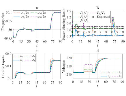
Figure 2: ($a$) Output frequencies $\omega_{i}(t)$; ($b$) Comparison between the actual ($P_{i}/P_{j}$) and the expected $k_{P_{i}}/k_{P_{j}}$, active power sharing ratio;($c$) Frequency SC control signals $\bar{\omega}_{i}(t)$; ($d$) Output voltages $v_{i}(t)$.

The simulation results in Fig. 2 confirm that the proposed frequency SC scheme effectively and robustly accomplishes the control objectives (6) and (7) despite the presence of communication time-varying delays, the MG operating working points changes due to either the activation of the voltage SC at $t=40\mathrm{s}$, or the disconnection/connection of the loads, resp., at $t=20\mathrm{s}$, and $t=35\mathrm{s}$. More specifically, when our frequency SC is inactive during Event 1, all the DGs frequencies deviate from their reference values, and the PC cannot succeed in restoring them (see Fig. 2 (a)). Once activated at $t=5s$, the proposed distributed SC not only robustly restores the DG frequencies to the expected values (see Fig. 2 (a)) but also preserves the active power sharing (see Fig. 2 (b)). Let us further note that, once at $t=75s$ $\omega_{0}$ is changed from $50Hz$ to $50.1Hz$, the MG correctly modifies its synchronous frequency while preserving the desired power sharing, cfr. Figs. 2 (a) and (b). Lastly, it is clear from Fig. 2 (c) that the frequency SC shows a satisfactory performance and smooth control signals.

VII Conclusions

This paper has proposed a frequency SC protocol for inverter-based microgrids accounting for disturbance terms and time-varying delays in the communication links. The method improves the current State of the Art because it is fully distributed, model-free, and robust against network-induced time-varying delays. Future research activities could be devoted to considering more general, possibly multi-time varying communication delays and switching topologies.

References

- [1] Josep M Guerrero et al. “Hierarchical control of droop-controlled AC and DC microgrids—A general approach toward standardization” In IEEE Transactions on industrial electronics 58.1 IEEE, 2010, pp. 158–172
- [2] S D’Silva, M Shadmand, S Bayhan and H Abu-Rub “Towards grid of microgrids: Seamless transition between grid-connected and islanded modes of operation. IEEE Open J Ind Electron Soc 2020; 1 (1): 66–81”, 2020
- [3] Florian Dörfler, John W. Simpson-Porco and Francesco Bullo “Breaking the Hierarchy: Distributed Control and Economic Optimality in Microgrids” In IEEE Transactions on Control of Network Systems 3.3, 2016, pp. 241–253 DOI: 10.1109/TCNS.2015.2459391
- [4] John W Simpson-Porco, Florian Dörfler and Francesco Bullo “Synchronization and power sharing for droop-controlled inverters in islanded microgrids” In Automatica 49.9 Elsevier, 2013, pp. 2603–2611
- [5] Fanghong Guo, Changyun Wen, Jianfeng Mao and Yong-Duan Song “Distributed secondary voltage and frequency restoration control of droop-controlled inverter-based microgrids” In IEEE Transactions on industrial Electronics 62.7 IEEE, 2014, pp. 4355–4364
- [6] Shichao Liu, Xiaoyu Wang and Peter Xiaoping Liu “Impact of communication delays on secondary frequency control in an islanded microgrid” In IEEE Transactions on Industrial Electronics 62.4 IEEE, 2014, pp. 2021–2031
- [7] Jingang Lai et al. “Droop-based distributed cooperative control for microgrids with time-varying delays” In IEEE Transactions on Smart Grid 7.4 IEEE, 2016, pp. 1775–1789
- [8] Jingang Lai, Xiaoqing Lu and Xinghuo Yu “Stochastic distributed frequency and load sharing control for microgrids with communication delays” In IEEE Systems Journal 13.4 IEEE, 2019, pp. 4269–4280
- [9] Boda Ning, Qing-Long Han and Lei Ding “Distributed finite-time secondary frequency and voltage control for islanded microgrids with communication delays and switching topologies” In IEEE Transactions on Cybernetics 51.8 IEEE, 2020, pp. 3988–3999
- [10] Amedeo Andreotti, Bianca Caiazzo, Alberto Petrillo and Stefania Santini “Distributed robust finite-time secondary control for stand-alone microgrids with time-varying communication delays” In IEEE Access 9 IEEE, 2021, pp. 59548–59563
- [11] Guannan Lou, Yinqiu Hong, Wei Gu and Jihua Xie “Event-triggered time synchronization strategy for distributed secondary control with consideration of time-varying delays” In CSEE Journal of Power and Energy Systems, 2022, pp. 1–10 DOI: 10.17775/CSEEJPES.2021.05640
- [12] Kai Zhao, Feng Xiao and Bo Wei “Distributed Asynchronous Event-Triggered Secondary Control of Microgrids with Time-Varying Communication Delays” In 2022 41st Chinese Control Conference (CCC), 2022, pp. 4637–4642 DOI: 10.23919/CCC55666.2022.9902187
- [13] Guanglei Zhao, Lanqing Jin, Hailong Cui and Yifeng Wang “Distributed Dynamic Event-Triggered Secondary Control for Islanded Microgrids with Disturbances and Communication Delays: A Hybrid Systems Approach” In IEEE Transactions on Industrial Informatics, 2022, pp. 1–10 DOI: 10.1109/TII.2022.3222378
- [14] Milad Gholami et al. “Robust consensus-based secondary voltage restoration of inverter-based islanded microgrids with delayed communications” In 2018 IEEE Conference on Decision and Control (CDC), 2018, pp. 811–816 IEEE
- [15] Alessandro Pilloni, Alessandro Pisano and Elio Usai “Robust finite-time frequency and voltage restoration of inverter-based microgrids via sliding-mode cooperative control” In IEEE Transactions on Industrial Electronics 65.1 IEEE, 2017, pp. 907–917
- [16] Ali Bidram, Ali Davoudi, Frank L Lewis and Josep M Guerrero “Distributed cooperative secondary control of microgrids using feedback linearization” In IEEE transactions on power systems 28.3 IEEE, 2013, pp. 3462–3470
- [17] Ke Shao et al. “Leakage-type adaptive state and disturbance observers for uncertain nonlinear systems” In Nonlinear Dynamics 105 Springer, 2021, pp. 2299–2311
- [18] Saleh Mobayen and Fairouz Tchier “Nonsingular fast terminal sliding-mode stabilizer for a class of uncertain nonlinear systems based on disturbance observer” In Scientia Iranica. Transaction D, Computer Science & Engineering, Electrical 24.3 Sharif University of Technology, 2017, pp. 1410–1418
- [19] Emilia Fridman and Yury Orlov “Exponential stability of linear distributed parameter systems with time-varying delays” In Automatica 45.1 Elsevier, 2009, pp. 194–201
- [20] Gang Chen and Frank L Lewis “Leader-following control for multiple inertial agents” In International Journal of Robust and Nonlinear Control 21.8 Wiley Online Library, 2011, pp. 925–942
- [21] Vadim Utkin and Jingxin Shi “Integral sliding mode in systems operating under uncertainty conditions” In Proceedings of 35th IEEE conference on decision and control 4, 1996, pp. 4591–4596 IEEE
- [22] Stephen Boyd, Laurent El Ghaoui, Eric Feron and Venkataramanan Balakrishnan “Linear matrix inequalities in system and control theory” SIAM, 1994