Variability in SSTc2d J163134.1-240100, a brown dwarf with quasi-spherical mass loss

Abstract

We report on a search for variability in the young brown dwarf SST1624 ($\sim$M7 spectral type, $M\sim 0.05\,M_{\odot}$), previously found to feature an expanding gaseous shell and to undergo quasi-spherical mass loss. We find no variability on timescales of 1-6 hours. Specifically, on these timescales, we rule out the presence of a period with amplitude $>1\%$. A photometric period in that range would have been evidence for either pulsation powered by Deuterium burning or rotation near breakup. However, we see a 3% decrease in the K-band magnitude between two consecutive observing nights (a 10 $\sigma$ result). There is also clear evidence for variations in the WISE lightcurves at 3.6 and 4.5$\,\mu m$ on timescales of days, with a tentative period of 6 d, and potentially long-term variations over time windows of years. The best explanation for the variations over days is rotational modulation due to spots. These results disfavour centrifugal winds driven by fast rotation as mechanism for the mass loss, which, in turn, makes the alternative scenario – a thermal pulse due to Deuterium burning – more plausible.

1 Introduction

Photometric monitoring has proven to be a useful observational tool in the exploration of brown dwarfs. When they are young, substellar objects often show variability due to magnetic activity, accretion, and disks, analogous to the more massive T Tauri stars (Scholz et al., 2009; Moore et al., 2019). For evolved brown dwarfs, photometric variability can signify the presence and evolution of clouds in the atmosphere (e.g. Metchev et al., 2015). Variability studies have been able to measure substellar rotation periods as a function of age (Bouvier et al., 2014), as well as constrain atmospheric properties and early evolutionary processes in brown dwarfs.

Thanks to numerous monitoring studies in the past twenty years, we know that young brown dwarfs show rotation periods ranging from a few hours to several days, whereas old evolved brown dwarfs generally have periods shorter than one day (Moore et al., 2019; Vos et al., 2022). At young ages, the shortest measured periods are around the physical limit – the period corresponding to breakup velocity, where centrifugal and gravitational forces are in balance at the equator. Rotation near or around breakup in young brown dwarfs has been reported by various authors, including Zapatero Osorio et al. (2003); Caballero et al. (2004); Scholz & Eislöffel (2005); Rodríguez-Ledesma et al. (2009). Such fast rotation will have significant effects on internal structure and early evolution, which needs to be accounted for in models (Yoshida, 2023).

The breakup velocity is calculated using $v=\sqrt{2GM/3R}$, following Porter (1996). The factor $2/3$ accounts for the fact that an object rotating at breakup will be oblate. For convenience, this corresponds to $P=0.14205\times R^{1.5}/M^{0.5}$. For substellar masses and ages 1-5 Myr, this yields breakup periods $>5$ h, as shown in Fig. 1 for two radii, typical for young brown dwarfs. As the objects age and contract, the breakup period drops with $\sim R^{1.5}$, but the rotation period (assuming angular momentum conservation) changes with $\sim R$, i.e. with increasing age the breakup period will drop further below the rotation period. As a result, field brown dwarfs which sometimes feature very short rotation periods of $\sim 1$ d (Tannock et al., 2021) are still significantly above breakup.

Another physical process that can be probed by photometric monitoring is pulsations. Brown dwarfs exhibit Deuterium burning during the first few Myrs of their existence, predicted to lead to a luminosity burst (Salpeter, 1992) and to radial or non-radial pulsations. Palla & Baraffe (2005) show in a stability analysis of Deuterium burning brown dwarfs the presence of fundamental modes with periods between 1 and 5 h. For 0.1$\,M_{\odot}$ stars, Rodríguez-López et al. (2012) find periods of modes excited by Deuterium burning of 4.2-5.2 h. A dedicated observational search for pulsation periods down to mmag precision, by Cody & Hillenbrand (2014), however, remained unsuccessful. In principle, some of the shortest photometric periods measured so far for brown dwarfs (see above) could be caused by pulsations. Most authors prefer, however, to interpret the periodic variability in young brown dwarfs as a result of rotation combined with magnetic surface spots. If pulsations were confirmed, it would open a new route to determine and ascertain fundamental properties in brown dwarfs during the phase of contraction.

In Figure 1 we include the estimated pulsation periods from Palla & Baraffe (2005) for ages of 1-3 Myr and substellar masses. As can be appreciated from this figure, the gap between pulsation periods and breakup periods widens with decreasing mass and increasing radius. A period below 4 h for such a young very low mass object would be very difficult to interpret as rotation period, offering a window to search for pulsations.

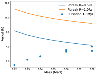
Figure 1: Estimated rotation period at breakup velocity (lines) and pulsation period (dots) for young brown dwarfs, as a function of mass. The breakup periods are shown for two different radii, consistent with the expected values for inflated, young substellar objects. Pulsation periods are the values given by Palla & Baraffe (2005) for ages between 1 and 3 Myr (their Table 1).

2 The target

SSTc2d J163134.1-240100 (hereafter SST1624) is a young brown dwarf in the Ophiuchus star forming complex, identified originally in the Spitzer ’Cores to Disks’ survey (Evans et al., 2009) as a faint, red young stellar object. In recent ALMA observations as part of the ODISEA program (Cieza et al., 2019), it was found to have a spherical, oblate envelope with a diameter of 200-300 AU, which shows the kinematics of an expanding shell (Ruíz-Rodríguez et al., 2022). The shell has been detected in ¹²CO, but not in the mm continuum. After correcting for extinction, the object has an infrared spectral energy distribution consistent with a diskless photosphere. This is very unusual – so far very few young brown dwarfs have been detected in CO with ALMA, and the ones that are, usually have an obvious disk (Ricci et al., 2014). On the other hand, numerous young brown dwarfs have been detected in the submm/mm continuum (Testi et al., 2016; Sanchis et al., 2020). We are thus confronted with an entirely new phenomenon that requires new ideas, continued exploration, and follow-up observations.

Ruíz-Rodríguez et al. (2022) determine the nature of the source based on KMOS spectra, and are careful to rule out alternative explanations, such as an AGB star in the background or a collapsing molecular core. Proper motions confirm that the object is indeed a member of the young population in Ophiuchus, with an age of $\sim 2$ Myr. Most likely, it is a 0.05$\,M_{\odot}$ brown dwarf, with mid/late M spectral type, overluminous, and seen through significant extinction of $A_{V}\sim 42$ mag. The best explanation for the gaseous expanding shell is strong, uncollimated mass loss. The age of the shell has been estimated kinematically to be $\sim 10^{4}$ years, a small fraction of the brown dwarf’s age, and its gas mass (under plausible assumptions) is $1.5\,M_{\oplus}$. The $4\,\sigma$ upper limit in the continuum observations corresponds to a dust mass of $<1\,M_{\oplus}$.

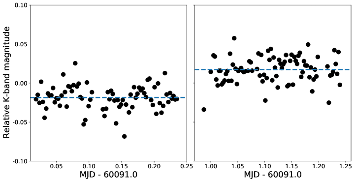
Figure 2: K-band lightcurve for SSTc2d J163134.1-240100, measured over two nights in May 2023. The magnitudes are measured relative to the average of four field stars. The blue dashed lines mark the average for a given night.

At this point the origin of the expanding shell is unknown. Ruíz-Rodríguez et al. (2022) suggest that the mass loss may be the result of a thermal pulse produced by the onset of Deuterium burning, analogous to the thermal pulses that drive mass loss in AGB stars Kerschbaum et al. (2017). Another option for a brown dwarf to eject a gaseous shell, originally suggested by Scholz & Eislöffel (2005), is through non-steady centrifugal winds caused by extremely fast rotation close to breakup speed – analogous to fast rotating OB stars (Porter, 1996). This would lead initially to a ring (a ’decretion disk’), expanding and dispersing to a quasi-spherical structure, consistent with the oblate shape of the shell of SST1624.

As pointed out in Section 1, both pulsation and fast rotation can cause a periodic flux change detectable by photometric monitoring, with the plausible periods for pulsations being shorter than those for fast rotation near breakup (see Figure 1). Testing for variability in SST1624 is therefore a promising way to explore the origin of its shell. This is the purpose of this paper.

For the record, Ruíz-Rodríguez et al. (2022) also discuss another option to explain the shell, the engulfment and consumption of a planetary companion. They deem this scenario as more exotic and less probable than the thermal pulse. As this idea would not produce a variability signature, we will not discuss it further here.

3 Observations and data reduction

3.1 K-band monitoring

We have monitored SST1624 over two nights, May 27th and May 28th 2023, with ESO/NTT and the infrared camera SOFI, under proposal ID 111.24GN. Overall, this observing run comprised three nights, but the third one was not usable due to clouds. In each of the two nights, we stayed on the target for 5-6 h, using the $K_{S}$ filter, DIT of 20 s, NDIT of 5 or 10, and employing random dithers. The data reduction includes cross-talk correction, flat fielding, sky subtraction, and bad-pixel correction. Individual exposures were combined, where necessary, to achieve a uniform total exposure time per frame of 200 s. On each image, we performed aperture photometry using photutils (Bradley et al., 2023) using a constant aperture of 10 pixels, which typically corresponds to 2-3 FWHMs of the seeing-limited PSF. This includes background subtraction, where the background was measured in an annulus around the source.

The raw lightcurve for SST1624 and all other stars in the field show substantial variations due to the change in airmass over the course of the night. We chose four stars in the same field that are brighter than our target, averaged their lightcurves, and subtracted this average from the target lightcurve (in units of magnitudes) to correct for atmospheric effects. The final lightcurve for SST1624 for those two nights is shown in Figure 2. We made sure that the lightcurve does not depend significantly on the choice of comparison stars, by checking the result with only a subset of them. We also checked the comparison stars against each other, and do not find any signs of variability in them. Using the comnparison stars for calibration, we determine that SST1624 has a K-band magnitude of $14.08\pm 0.05$ in the 2MASS system, consistent with its 2MASS value of 14.06.

3.2 Archival WISE lightcurves

We also obtain the WISE lightcurve at 3.6 (W1) and 4.5$\,\mu m$ (W2) for SST1624 from the ’ALLWISE Multiepoch Photometry Table’ (Cutri et al., 2021) and the ’NEOWISE-R Single Exposure (L1b) Source Table’ (Mainzer et al., 2014). The ALLWISE table contains 23 epochs for this source within 200 d, starting at MJD55254. With one exception, all of these measurements are concentrated in two 24 h spans, separated by $\sim 180$ d, and shown in Figure 3.

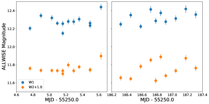
Figure 3: ALLWISE lightcurve for SSTc2d J163134.1-240100, comprising 22 of the 23 datapoints in the archive. The W2 magnitudes are offset by 1.0 mag for clarity.

NEOWISE-R provides 214 good detections (as of June 2023), over a duration of $\sim 3000$ d, starting at MJD 56700.0, with 18 day-long spans covered by about 10 datapoints each. Again the measurements are available for the two bands W1 and W2. We note that this lightcurve ends at MJD 59803 which corresponds to December 2022, a few months prior to our dedicated K-band monitoring. More NEOWISE-R data for this source will become available in the coming years. The full lightcurve is shown in Figure 4.

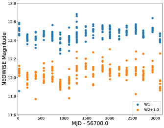
Figure 4: NEOWISE-R lightcurve for SSTc2d J163134.1-240100, comprising 214 datapoints. A few outliers are not shown here. The W2 magnitudes are offset by 1.0 mag for clarity. The typical photometric error is 0.03 mag.

4 Lightcurve analysis

4.1 K-band monitoring

The lightcurve we obtained from the SOFI observations appears unremarkable. By eye, it shows noise around a flat mean, in each of the two consecutive nights, as can be appreciated from Figure 2. There is no obvious structure, in particular no obvious periodic variability. The standard deviation is 1.5 and 1.6%, for night 1 and night 2 respectively.

To check for gradual trends, we fit the data in individual nights with a line. In the first night, the best fitting slope is -0.006 mag/day, which is consistent with zero. In the second night, the fit gives 0.026 mag/day or 0.010 mag/day when ignoring the very first outlying datapoint. Again this would be consistent with zero over a time window of 6 h.

There is, however, a significant offset between the mean magnitude in the two nights; the object dimmed by 3% over the course of 1 d, a 10 $\sigma$ detection given the error of the mean in the lightcurves in individual nights. This shift is not seen in individual comparison stars. Given that the observing setup was identical in both nights, and the range of airmasses was the same, too, this dimming is likely caused by intrinsic variability in our target. We note that this offset, in combination with the linear slopes measured for individual nights, could be consistent with a sinusoidal variation – in that case the object would be near maximum in the first night; the period would be on the order of days.

We devised a simple, robust test to check for the presence of a period in noisy data by comparing the variance in the lightcurve before and after subtracting a periodicity, a procedure hereafter called Max-F. We define a range of test periods, from 0.1 h to 6 h in steps of 0.05 h. For each test period we calculate the phases of the datapoints (between 0.0 and 1.0). Then we subtract sinecurves, varying the amplitude between 5% and 100% the maximum range of datapoints (in steps of 5%) and varying the phase of the zeropoint (in steps of 0.01). We record the standard deviation of the lightcurve for each subtracted sinecurve, $\sigma_{P,i}$, and the variance ratio $F=\sigma^{2}/\sigma_{P,i}^{2}$. We find the maximum value for $F_{P}$ for each period, and plot that as a function of period. This procedure gives us a measure of the maximum fraction of the noise that could be explained by the presence of a sinusoidal period. The routine constitutes in essence an F-test for the equality of variances. For normally distributed datasets, the quantity $F$ should follow an F-distribution (hence the name). For our case with $N\sim 80$, a F-value of $>1.5$ would mean that the two variances are significantly different with a false alarm probability $<5$%.

For the first night, we find that the maximum value of $F$ is 1.16, for a period of 3.0 h. For the second night, the maximum $F$ is 1.22, but only for periods shorter than 1 h; for longer periods the maximum is 1.03. Taken together, these results are consistent with the variances being equal before and after period subtraction, i.e. with the non-detection of a period. It also means that at most a few percent of the variance can be explained by a potential period.

We applied the same test after injecting a period into the lightcurve, and find for periods of 1-5 h and amplitudes of 0.01 mag (1%), $F$ would be $\sim 1.3$, depending slightly on period, with a clearly defined maximum at the injected period value. The injected period is then also visible by eye in the lightcurve. This demonstrates that periods with these characteristics are recovered by Max-F, but are not present in the original dataset.

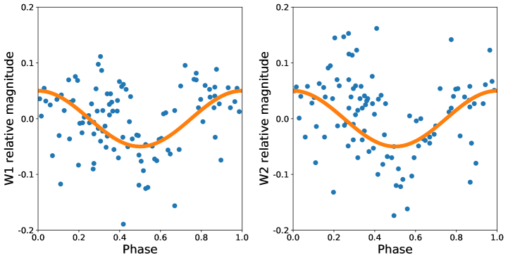
Figure 5: The first half of the NEOWISE-R dataset, plotted in phase to a period of $P=6.0\,d$. Overplotted is the sinecurve with an amplitude of 0.05 mag to guide the eye. The typical photometric error is 0.03 mag.

4.2 WISE lightcurves

In the ALLWISE and NEOWISE-R lightcurves, SST1624 shows significant variability, dominated by modulations on timescales of days, with typical peak-to-peak amplitudes of 0.1-0.3 mag (see Figures 3 and 4). For comparison, the average photometric error is 0.03 mag for a single epoch. Taken the two datasets together, the variability is sustained over more than 12 years. Over long timescales, the brightness of this object appears to be mostly stable within the margins of the intra-night variations.

The NEOWISE-R dataset allows a more detailed analysis. It consists of 18 sets of points, each measured within a couple of days, and separated by about 180 d (see Figure 4). Given this sampling, the NEOWISE-R lightcurve is not sensitive to the short timescales covered with our K-band monitoring, but can be useful to pick up variability on timescales ranging from days to years.

We carried out the same Max-F test we described in the previous section, to search for a possible periodicity. For periods ranging from 1 to 10 d, and for the full NEOWISE-R lightcurves, the maximum $F$ is 1.08 in W1 and 1.14 in W2. In both cases this maximum is achieved for periods of 6 d. We noticed that the maximum $F$ increases significantly if we run the test only on the first half of the dataset. For band W1, we obtain peaks at 3.5, 4.0, 5.9, 6.1, all with $F>1.25$. For W2, the highest peak is for $P=6.0$ d, with $F\sim 1.25$. As a reminder, this means that the variance is reduced to 80% ($1/1.25$) when subtracting this specific periodicity. However, for this value of $F$ there is still a substantial probability (12%) that the two variances before and after subtracting the period are equal (assuming normally distributed samples).

In Figure 5 we show the first half of the NEOWISE-R datapoints plotted in phase for $P=6.0$ d. As can be appreciated from this figure, the periodicity looks plausible by eye. It is conceivable that parts or all of the variability seen in WISE data is caused by a flux modulation with a period of 6 d and an amplitude of $\pm 0.05$ mag.

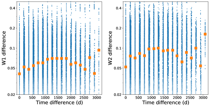
Figure 6: Differences between NEOWISE-R magnitudes, as a function of time difference, for the two bands separately (W1 in the right panel, W2 in the left panel). The orange square show the median for an interval of $\pm 10$ d around a given time difference. The typical error in the magnitude difference is 0.04 mag.

To quantify typical timescales of variability from the NEOWISE-R lightcurve, we calculated the difference between each pair of datapoints $\Delta M$, and plot this over their time difference $\Delta t$ (see Figure 6). This analysis was carried out for the two bands separately, but they both give very similar results. As can be seen in the figure, the overall range of $\Delta M$ is not a strong function of time difference $\Delta t$. The median of $\Delta M$ (shown as orange squares) is 0.04-0.05 for the shortest $\Delta t$ (hours to days), slightly larger than the photometric error of 0.03 mag. Thus, this test confirms that most of the variability occurs on timescales of days, consistent with the possible periodicity discussed above. The median of $\Delta M$ increases gradually to 0.07-0.10 up to $\Delta t\sim 1000$ d, where it plateaus. This may show that additional long-term variability is introduced on timescales of several years.

5 Summary and discussion

SST1624 is a brown dwarf with quasi-spherical mass loss, a unique object that may give us insights into important aspects of the early evolution of substellar objects. Two possible mechanisms to explain the mass loss are a thermal pulse from the onset of Deuterium burning or centrifugal winds due to very fast rotation. In both cases, we may expect variability in short timescales, either due to pulsation or rotation.

We present here infrared lightcurves for SST1624 from newly obtained high-cadence K-band ESO/NTT observations and from the publicly available ALLWISE and NEOWISE-R archives. Overall, there is clear evidence for variability in SST1624, on timescales of $>6$ h to days, measured at 2-4.5$\,\mu m$ in all available datasets. On the other hand, we rule out variability, and specifically the presence of a photometric period on timescales $<6$ h, for amplitudes $>1$%. We do identify a possible photometric period of 6 d in the first half of the NEOWISE-R dataset, seen at 3.6 and 4.5$\,\mu m$. There may be additional variability on timescales of years.

We note that our target was included in the variability search by Park et al. (2021) using the first 6.5 yr of NEOWISE data – no variability was found. This study, however, was only focused on long-term variations over timescales longer than days. Also, the NEOWISE-R dataset is now significantly longer.

The variability on day-long timescales, and the tentative period of 6 d, is best explained by magnetic activity, i.e. spots on the surface co-rotating with the object. This implies that the rotation period for this object is in the order of a few days. Period and amplitude are comparable to what has been found for young brown dwarfs (e.g. Scholz & Eislöffel, 2005; Moore et al., 2019). The WISE lightcurve is very clumpy, with gaps of 6 months between clumps of data. Over such long timescales, the spot distribution can change, leading to phaseshifts and amplitude changes. For timescales around 1 d, the number of datapoints is very low. These two characteristics in combination hamper any period search and can easily explain why the period is not apparent in the entire dataset. To robustly confirm the tentative period of 6 d as the rotation period, a dedicated monitoring campaign over at least one week, if possible without daytime gaps, would be needed.

The only other conceivable explanation for the observed variability is the presence of some residual circum-sub-stellar dust close to the object that causes variability through obscuration (Scholz et al., 2009) – however, the lack of an infrared excess and the lack of a mm continuum detection renders this interpretation unlikely.

Coming back to the topic of the quasi-spherical mass loss, the unique feature of this object: With our dedicated K-band monitoring, we set out to find periods on timescales of hours, to distinguish between pulsations (1-4 h) and rotation near breakup ($>5$ h). Since we did not find periods on these timescales, the available data does not give us a definitive answer on the cause of the mass loss. Having said that, the fact that there is clear variability over timescales of days, best explained by rotational modulations, would imply that the object is in fact not rotating close to breakup. Rotation periods of several days are at the high end of the period distribution for young brown dwarfs, see Figure 13 in Moore et al. (2019). This renders the scenario where the mass loss is due to the onset of Deuterium burning, favoured and worked out by Ruíz-Rodríguez et al. (2022), more likely. The absence of a pulsation period in the lightcurves could mean that the object has stopped pulsating since the ejection of the shell, or that the pulsations happen at amplitudes below 1%, as it is likely the case for pulsating M dwarfs (Rodríguez et al., 2016; Rodríguez-López, 2019).

This brown dwarf deserves further time-series observations to a) verify the rotation period and b) search for pulsations with higher precision. As the first brown dwarf with observed quasi-spherical mass loss, this source may present an opportunity to learn more about the hitherto unexplored aspects in the early evolution of brown dwarfs. Deuterium burning is a common feature in all young brown dwarfs, and if this leads to mass loss, either sustained, or in bursts, it would affect the substellar mass function and angular momentum evolution. Exploring the prevalence and duration of substellar mass loss is an important task for future work.