Actions Speak What You Want: Provably Sample-Efficient Reinforcement Learning of the Quantal Stackelberg Equilibrium from Strategic Feedbacks

Siyu Chen   Mengdi Wang   Zhuoran Yang Department of Statistics and Data Science, Yale University. Email: siyu.chen.sc3226@yale.edu.Department of Electrical and Computer Engineering, Princeton University. Email: mengdiw@princeton.edu.Department of Statistics and Data Science, Yale University. Email: zhuoran.yang@yale.edu.
Abstract

We study reinforcement learning (RL) for learning a Quantal Stackelberg Equilibrium (QSE) in an episodic Markov game with a leader-follower structure. In specific, at the outset of the game, the leader announces her policy to the follower and commits to it. The follower observes the leader’s policy and, in turn, adopts a quantal response policy by solving an entropy-regularized policy optimization problem induced by leader’s policy. The goal of the leader is to find her optimal policy, which yields the optimal expected total return, by interacting with the follower and learning from data. A key challenge of this problem is that the leader cannot observe the follower’s reward, and needs to infer the follower’s quantal response model from his actions against leader’s policies. We propose sample-efficient algorithms for both the online and offline settings, in the context of function approximation. Our algorithms are based on (i) learning the quantal response model via maximum likelihood estimation and (ii) model-free or model-based RL for solving the leader’s decision making problem, and we show that they achieve sublinear regret upper bounds. Moreover, we quantify the uncertainty of these estimators and leverage the uncertainty to implement optimistic and pessimistic algorithms for online and offline settings. Besides, when specialized to the linear and myopic setting, our algorithms are also computationally efficient. Our theoretical analysis features a novel performance-difference lemma which incorporates the error of quantal response model, which might be of independent interest.

1 Introduction

Multi-agent reinforcement learning (RL) (Busoniu et al., 2008; Zhang et al., 2021) studies sequential decision making problems where multiple agents interact with each other. Such a problem is often modeled as a Markov game, where at each timestep, each agent takes an action at the current state of the environment, receives an immediate reward, and the environment moves to a new state according to a Markov transition kernel. Here the agents affect each other because the rewards and state transitions depend on the actions of all players. The goal of each agent is to learn her optimal policy that maximizes her expected total return, in the presence of strategic plays of other agents.

Compared with single-agent RL, one of the most salient challenges of multi-agent RL is nonstationarity. That is, from the perspective of each agent, she faces a Markov decision process (MDP) induced by the policy of the other agents, which changes abruptly once the other agents adopt new policies. To deal with such a challenge, most of the existing literature either (i) assumes a central controller that learns the policies for all agents, or (ii) designs decentralized methods based on adversarial bandits algorithms (see Section 2 for details). The way these works deal with nonstationarity is rather “passive”. In particular, nonstationarity is out of the scope given (i), and (ii) assumes the other agents change arbitrarily and only hopes to compete against the best fixed policy in hindsight.

In contrast, an “active” approach of dealing nonstationarity would actively infer how other agents adjust their policies from their history actions, and leveraging such information to better design her own policy. Such an active approach is particularly promising in human-robot interaction, where we aim to train robots to better assist human by learning from human feedback.

In this work, we aim to design provably efficient RL algorithms for Markov games that actively address the challenge of nonstationarity. As an initial attempt, we focus on the setting of a two-player Markov games with a leader-follower structure. In specific, in such a game, the leader takes on the role of the primary decision-maker who commits to a policy π𝜋\pi upfront, while the follower, knowing π𝜋\pi, chooses a best-response policy νπsuperscript𝜈𝜋\nu^{\pi} that maximizes his expected rewards. Here we assume the follower’s response νπsuperscript𝜈𝜋\nu^{\pi} is unique, which is obtained by solving an entropy-regularized MDP induced by π𝜋\pi. Here νπsuperscript𝜈𝜋\nu^{\pi} is also called the quantal response to leader’s policy π𝜋\pi. We allow the follower to be either myopic, considering only the immediate reward, or farsighted, planning ahead across all future steps. The leader’s objective is to find her optimal policy πsuperscript𝜋\pi^{*} such that the policy pair (π,νπ)superscript𝜋superscript𝜈superscript𝜋(\pi^{*},\nu^{\pi^{*}}) optimizes her expected total rewards, and (π,νπ)superscript𝜋superscript𝜈superscript𝜋(\pi^{*},\nu^{\pi^{*}}) is called a quantal Stackelberg equilibrium (QSE) (Başar and Olsder, 1998; McKelvey and Palfrey, 1995). The objectives of the leader and the follower are misaligned as their reward functions u𝑢u and r𝑟r are different. Our goal is to design online and offline RL algorithms for the leader under the episodic and function approximation setting, based only on information available to the leader, i.e., states, joint actions, and the leader’s rewards. In particular, the leader only observes the follower’s actions, not rewards.

To efficiently learn πsuperscript𝜋\pi^{*}, the leader needs to efficiently optimize her own expected return by strategically guiding the follower’s behavior, which necessitates actively learning the follower’s quantal response mapping from the data. Learning a QSE poses a few unique challenges. (a) First, the leader must infer the follower’s quantal response mapping from follower’s actions, which requires building a response model and inferring follower’s reward function by observing how the follower responds to different leader policies. Such a challenge is exacerbated when the follower is farsighted. (b) Second, QSE is posed as the solution to a bilevel optimization where the leader optimizes her policy subject to the constraint that the follower adopts the quantal response policy. Characterizing the performance of the leader’s learned policy requires novel analysis that bridges the upper and lower-level problems. In specific, we need to determine how the error of the inferred quantal response affects the performance of the learned policy. (c) Third, we need to understand how to incentivize exploration in the online setting or how to guard against insufficient data coverage in the offline setting, in the presence of an inaccurate response model. Handling this challenge requires modifying the optimism/pessimism principle for the problem of learning a QSE.

We successfully tackle these challenges and establish provably sample-efficient RL algorithms for both online and offline settings, in the context of function approximation, where the follower can be either myopic or farsighted. In specific, our algorithms are based on (i) a model-based approach for learning the follower’s quantal-response via maximum likelihood estimation (Challenge (a)), and (ii) a single-agent reinforcement learning method for leader’s decision making problem. In specific, for a myopic follower, we adopt a model-free least-squares value iteration (LSVI) (Sutton and Barto, 2018) approach to learn the leader’s optimal value function. For a farsighted follower, we leverage model-based RL to learn the transition model and the leader’s reward function. In addition, to promote exploration in the online setting, we construct confidence sets for both the response model and leader’s value function (or transition and reward model), and propose to update the leader’s policies via optimistic planning (Auer et al., 2008). Such an algorithm can be easily modified for the offline setting via pessimistic planning (Challenge (c)). Both these algorithms are able to incorporate general function approximation. Furthermore, in the special case with myopic follower and linear function approximation, we establish variants of optimistic and pessimistic algorithms that can be efficiently implemented using bonus and penalty functions. Furthermore, we prove that all of these methods enjoy sublinear regret or suboptimality bounds, hence proving statistical efficiency. In the case with general function approximation, we introduce novel eluder dimensions that captures the challenge of exploration for learning a QSE. Finally, to characterize the suboptimality of leader’s policy, we establish a novel performance difference lemma which relates the suboptimality of the learned policy to the Bellman error of the upper level problem and the estimation error of the response model in the lower level problem (Challenge (b)). Such a result might be of independent interest.

Our Contributions. In summary, this work proposes provably sample-efficient algorithms for learning the QSE in an episodic Markov game with a leader-follower structure. In such a game, when the leader announces her policy, the follower adopts the corresponding quantal response, and the leader only observes the follower’s actions but not rewards. To address the challenge of nonstationarity, the leader needs to actively infer how the follower reacts to her announced policy, and leverage such information to drive the game towards the QSE. We successfully address such a challenge for both online and offline RL settings with linear and general function approximation. We also allow the follower to be both myopic and farsighted. Specifically, our contributions are three-fold.

  • (i)

    First, for the case of a linear Markov game with a myopic follower, we establish sample-efficient RL algorithms for both the offline and online settings. These algorithms are based on the principle of pessimism/optimism in the face of uncertainty, where we quantify the estimation uncertainty of leader’s value function and follower’s quantal response model. Thanks to the linear structure, both the offline and online algorithms have versions that are computationally efficient (Algorithm 1 with S3 and Algorithm 3 with S5).

  • (ii)

    Second, for the case with general function approximation, we propose provably sample-efficient algorithms for both the online and offline settings, where the follower is allowed to be either myopic or farsighted. In particular, in the case with a myopic follower, our algorithms combine model-free value estimation for the leader and maximum likelihood estimation of the follower’s quantal response mapping (Algorithm 2 and Algorithm 4). For the case with a farsighted follower, we propose model-based algorithms by combining pessimism and optimism with maximum likelihood estimation for Markov game model (Algorithm 5 and Algorithm 6). We prove that these algorithm are all sample-efficient by establishing upper bounds on the suboptimality or cumulative regret.

  • (iii)

    Third, we establish a novel performance difference lemma which relates the suboptimality of the leader’s policy to leader’s Bellman error and the error incurred in estimating the follower’s quantal response model, which is measured in terms of the total variation (TV) distance. (See (4.1) or Lemma B.1 for details.) Moreover, due to the nonlinear nature of the quantal response mapping, we further expand the estimation error of the quantal response model into a first-order and a second-order term, which can be further controlled by the maximum likelihood analysis. (See (4.4) or Lemma B.2 for details.) From the lens of bilevel optimization, our regret analysis connects the Bellman error in the upper level with the quantal response error in lower level, which might be of independent interest.

2 Related Works

Our work is most related to works that learn Stackelberg equilibria in (Markov) games via online RL (Bai et al., 2021; Zhong et al., 2023; Kao et al., 2022; Zhao et al., 2023). All of these works assume the follower is myopic and perfectly rational. In the following, we discuss these works in detail. Moreover, our work adds to the large body of literature of of single-agent and multi-agent online and offline RL, as well as the literature of maximum entropy inverse RL.

Online Single-Agent Reinforcement Learning with Function Approximation. Our works is related to the line of work that designs provably sample-efficient RL algorithms for MDPs in the context of function approximation. Various works propose RL algorithms that focus on the linear case, (Wang et al., 2019; Yang and Wang, 2019; Cai et al., 2020; Jin et al., 2020; Zanette et al., 2020; Ayoub et al., 2020; Modi et al., 2020; Yang et al., 2020; Zhou et al., 2021a). Among these works, our work is most related to Jin et al. (2020). In particular, the linear Markov game model we study for the linear case is a direct extension of the linear MDP model in Jin et al. (2020). Moreover, the bonus function Γh(1)superscriptsubscriptΓ1\Gamma_{h}^{(1)} and the U𝑈U-function (which plays the same role as the Q-function in single-agent RL) constructed in (6.1) are the same as the UCB bonus function and the optimistic value function in Jin et al. (2020). Furthermore, more recently, there is a line of research that study sample-efficient RL in the context of general function approximation. See, e.g., Jiang et al. (2017); Sun et al. (2019); Wang et al. (2020); Jin et al. (2021a); Du et al. (2021); Dann et al. (2021); Zhong et al. (2022b); Foster et al. (2021, 2023) and the references therein. Among these works, our work is particularly related to the work of Jin et al. (2021a), which proposes a model-free algorithm named GOLF that is an optimistic variant of least-squares value iteration. For the case of online RL with general function approximation, our algorithm for updating the leader’s value functions is based on a modified version of GOLF, where we additionally take into account the estimation uncertainty of the follower’s quantal response model. Moreover, Jin et al. (2021a) introduce the Bellman eluder dimension that characterizes the exploration difficulty of the MDP problem. In the regret analysis, we introduce similar notions of eluder dimension for learning the leader’s optimal policy. In particular, we introduce two versions of eluder dimensions that captures the complexity of leader’s Bellman error and the follower’s quantal response error.

Online Multi-Agent Reinforcement Learning. Our work is also related to the literature on online multi-agent RL. Most of the existing research focus on learning Markov perfect equilibria in two-agent zero-sum Markov games or correlated or coarse correlated equilibria in general-sum Markov games. These works can be divided into two strands depending whether the proposed algorithm is centralized or decentralized. When there is a central controller that learns the policies of all agents, a few recent works propose extensions of single-agent RL algorithms to Markov games based on the principle of optimism in the face of uncertainty (Bai et al., 2020; Bai and Jin, 2020; Liu et al., 2020; Jin et al., 2021c; Huang et al., 2021; Xiong et al., 2022; Xie et al., 2020; Chen et al., 2021). The second strand of research develops decentralized online RL algorithm for a single-agent of in a Markov games. See, e.g., Jin et al. (2021b); Liu et al. (2022); Zhan et al. (2022); Song et al. (2021); Tian et al. (2021); Mao and Başar (2023); Erez et al. (2022); Wang et al. (2023); Cui et al. (2023) and the references therein. The algorithms proposed in most of these works handle the nonstationary due to other agents by leveraging techniques from adversarial bandit literature.

Our work is more related to works that learns Stackelberg equilibria in (Markov) games via online RL (Bai et al., 2021; Zhong et al., 2023; Kao et al., 2022; Zhao et al., 2023). All of these works assume the follower is myopic and perfectly rational. In specific, Bai et al. (2021); Zhao et al. (2023) focus on the static setting. Bai et al. (2021) consider a centralized setting where central controller can determines the actions taken by both the leader and the follower. Zhao et al. (2023) assume the follower is omniscient in the sense that the follower always plays the best response policy, which is similar to our setting. They show that when the follower is perfectly rational, the regret of the leader exhibits different scenarios depending on the relationship between the leader’s and follower’s rewards. Besides, Kao et al. (2022) assume that the leader and follower are cooperative and design a decentralized algorithm for both the leader and follower, under the tabular setting. Zhong et al. (2023) study online and offline RL for the leader, assuming the follower’s reward function is known, and thus the best response of the follower is known to the leader.

Offline Reinforcement Learning with Pessimism. Our work is also related to the recent line of research on the efficacy of pessimism in offline RL. See, e.g., (Yu et al., 2020; Kidambi et al., 2020; Kumar et al., 2020; Buckman et al., 2020; Jin et al., 2021d; Rashidinejad et al., 2021; Zanette et al., 2021; Uehara and Sun, 2021; Xie et al., 2021; Lyu et al., 2022; Shi et al., 2022; Yan et al., 2022; Zhong et al., 2022a; Cui and Du, 2022b, a; Yu et al., 2022; Zhang et al., 2023) and the references therein for algorithms for MDP or Markov games based on the pessimism principle. Among these works, our work is particularly related to Jin et al. (2021d); Xie et al. (2021); Uehara and Sun (2021); Yu et al. (2022). In particular, in the case of myopic follower and linear function approximation, our offline RL is based on the LSVI-LCB algorithm introduced in (Jin et al., 2021d), which uses a penalty function to perform pessimism. Furthermore, in the case of myopic follower and general function approximation, our algorithm is an extension of the value-based pessimistic algorithm proposed in Xie et al. (2021) to leader-follower game, and when the follower is farsighted, our algorithm is an extension of the model-based pessimistic algorithm proposed in Uehara and Sun (2021). Finally, Yu et al. (2022) studies a different leader-follower game with myopic followers and they propose a model-based and pessimistic algorithm that leverages nonparametric instrumental variable regression.

Maximum Entropy Inverse Reinforcement Learning (MaxEnt IRL). Our approach of learning the quantal response mapping via maximum likelihood estimation is related to the existing works on MaxEnt IRL, where the goal is to recover the reward function from expert trajectories based on an energy-based model (Ziebart et al., 2008; Neu and Szepesvári, 2009; Ziebart et al., 2010; Choi and Kim, 2012; Gleave and Toyer, 2022; Zhu et al., 2023). Among these works, our work is more relevant to Zhu et al. (2023), which establishes the sample complexity of MaxEnt IRL, and learning reward functions from comparison data in both bandits and MDPs. The analysis in Zhu et al. (2023) builds upon the body of literature on learning from comparisons (Bradley and Terry, 1952; Plackett, 1975; Luce, 2012; Hajek et al., 2014; Shah et al., 2015; Negahban et al., 2012). Zhu et al. (2023) considers maximum likelihood estimation with linear rewards, whereas we also consider general function approximation. More importantly, learning quantal response model from follower’s actions is only the lower level problem, and our eventual goal is to learn the optimal policy of the leader. Such a bilevel structure is not considered in Zhu et al. (2023).

3 Preliminaries

Notations. We denote by 𝕊+dsuperscriptsubscript𝕊𝑑\mathbb{S}_{+}^{d} the class of d𝑑d-dimensional symmetric nonnegative definite matrices, (𝒳)𝒳{\mathcal{F}}({\mathcal{X}}) the class of measurable functions on space 𝒳𝒳{\mathcal{X}}, [N]={1,,N}delimited-[]𝑁1𝑁[N]=\{1,\dots,N\}, Δ(𝒳)Δ𝒳\Delta({\mathcal{X}}) the probability space on 𝒳𝒳{\mathcal{X}}, Cov[v]Cov𝑣\operatorname{\rm Cov}[v] the covariance matrix for random vector v𝑣v, and P\left\|\cdot\right\|_{P} the vector norm induced by P𝕊+d𝑃superscriptsubscript𝕊𝑑P\in\mathbb{S}_{+}^{d}. We denote by less-than-or-similar-to\lesssim the inequality relationship up to some constants and logarithmic factors. We denote by |||{\mathcal{B}}| the size of a class {\mathcal{B}}.

3.1 Episodic Leader-Follower Markov Game

We consider an episodic two-player Markov game between a leader and a follower, denoted by M={𝒮,𝒜,,H,ρ0,P,u,r}.𝑀𝒮𝒜𝐻subscript𝜌0𝑃𝑢𝑟M=\{{\mathcal{S}},{\mathcal{A}},{\mathcal{B}},H,\rho_{0},P,u,r\}. Here 𝒮𝒮{\mathcal{S}} denotes the state space, 𝒜𝒜{\mathcal{A}} and {\mathcal{B}} are the action spaces of the leader and follower, respectively, H𝐻H is the horizon length. In addition, P={Ph:𝒮×𝒜×Δ(𝒮)}h[H]𝑃subscriptconditional-setsubscript𝑃𝒮𝒜Δ𝒮delimited-[]𝐻P=\{P_{h}\colon{\mathcal{S}}\times{\mathcal{A}}\times{\mathcal{B}}\rightarrow\Delta({\mathcal{S}})\}_{h\in[H]} are the transition kernels, and u={uh:𝒮×𝒜×[0,1]}h[H]𝑢subscriptconditional-setsubscript𝑢𝒮𝒜01delimited-[]𝐻u=\{u_{h}\colon{\mathcal{S}}\times{\mathcal{A}}\times{\mathcal{B}}\rightarrow[0,1]\}_{h\in[H]} and r={rh:𝒮×𝒜×[0,1]}h[H]𝑟subscriptconditional-setsubscript𝑟𝒮𝒜01delimited-[]𝐻r=\{r_{h}\colon{\mathcal{S}}\times{\mathcal{A}}\times{\mathcal{B}}\rightarrow[0,1]\}_{h\in[H]} are the reward functions of the leader and the follower, respectively. In such a game, for any h[H]delimited-[]𝐻h\in[H], at step hh, both the leader and follower observe the current state sh𝒮subscript𝑠𝒮s_{h}\in{\mathcal{S}}, take actions ah𝒜subscript𝑎𝒜a_{h}\in{\mathcal{A}} and bhsubscript𝑏b_{h}\in{\mathcal{B}}, receives rewards uh(sh,ah,bh)subscript𝑢subscript𝑠subscript𝑎subscript𝑏u_{h}(s_{h},a_{h},b_{h}) and rh(sh,ah,bh)subscript𝑟subscript𝑠subscript𝑎subscript𝑏r_{h}(s_{h},a_{h},b_{h}) respectively, and the environment moves to a new state sh+1Ph(|sh,ah,bh)s_{h+1}\sim P_{h}(\cdot{\,|\,}s_{h},a_{h},b_{h}). Here the initial state s1ρ0Δ(𝒮)similar-tosubscript𝑠1subscript𝜌0Δ𝒮s_{1}\sim\rho_{0}\in\Delta({\mathcal{S}}) and the game terminates after sH+1subscript𝑠𝐻1s_{H+1} is generated.

Leader-Follower Structure and Policies. We assume that the leader is a more powerful player who is able to coordinate the follower’s behaviors. In specific, at the beginning of the game, the leader announces her policy π={πh}h[H]𝜋subscriptsubscript𝜋delimited-[]𝐻\pi=\{\pi_{h}\}_{h\in[H]} for the entire game to the follower, where πh:𝒮𝒜:subscript𝜋𝒮𝒜\pi_{h}\colon{\mathcal{S}}\rightarrow{\mathscr{A}} maps the current state to an element in 𝒜𝒜{\mathscr{A}}. Here 𝒜={Δ(𝒜)}𝒜Δ𝒜{\mathscr{A}}=\{{\mathcal{B}}\rightarrow\Delta({\mathcal{A}})\} denotes the set of functions that maps each action b𝑏b of the follower to a distribution over 𝒜𝒜{\mathcal{A}}. In other words, each element α𝒜𝛼𝒜\alpha\in{\mathscr{A}} can be viewed as a prescription (Nayyar et al., 2014) that specifies the leader’s action contingent on the follower’s action. When the leader announces π𝜋\pi beforehand, she informs the follower how she will choose her action ahsubscript𝑎a_{h} at each state shsubscript𝑠s_{h}, given the follower’s action bhsubscript𝑏b_{h}. To simplify the notation, in the sequel, we regard πhsubscript𝜋\pi_{h} as a function πh(|sh,bh)Δ(𝒜)\pi_{h}(\cdot{\,|\,}s_{h},b_{h})\in\Delta({\mathcal{A}}), which specifies the distribution of ahsubscript𝑎a_{h}.111Here we assume that the leader is a more powerful player in the sense that her policy π𝜋\pi takes the follower’s action bhsubscript𝑏b_{h} as an input, although she does not observe bhsubscript𝑏b_{h} when announcing π𝜋\pi. This can be easily modified for a slightly weaker leader, whose policies π𝜋\pi does not depend on bhsubscript𝑏b_{h}. That is, πh(|sh)\pi_{h}(\cdot{\,|\,}s_{h}) maps shsubscript𝑠s_{h} to a distribution over 𝒜𝒜{\mathcal{A}}.

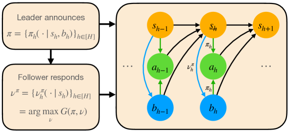
Furthermore, the follower’s policy is denoted by ν={νh}h[H]𝜈subscriptsubscript𝜈delimited-[]𝐻\nu=\{\nu_{h}\}_{h\in[H]}, where νh:𝒮Δ():subscript𝜈𝒮Δ\nu_{h}\colon{\mathcal{S}}\rightarrow\Delta({\mathcal{B}}) specifies how the follower takes action bhsubscript𝑏b_{h} at state shsubscript𝑠s_{h}. With the leader-follower structure, the actions {ah,bh}subscript𝑎subscript𝑏\{a_{h},b_{h}\} are generated as follows. At the beginning, the leader announces her policy π𝜋\pi. The follower observes π𝜋\pi and chooses a policy ν𝜈\nu. For any h[H]delimited-[]𝐻h\in[H], at the hh-th time step, the leader commits to the announced policy and samples αh=πh(sh)subscript𝛼subscript𝜋subscript𝑠\alpha_{h}=\pi_{h}(s_{h}) at state shsubscript𝑠s_{h}, the follower chooses bhνh(|sh)b_{h}\sim\nu_{h}(\cdot{\,|\,}s_{h}), and then the leader executes ahαh(|bh)=πh(|sh,bh)a_{h}\sim\alpha_{h}(\cdot{\,|\,}b_{h})=\pi_{h}(\cdot{\,|\,}s_{h},b_{h}). The structure of this Markov game is depicted in Figure 1.

Refer to caption
Figure 1: Structure of the Markov game. After the leader announces her H𝐻H-step policies, the follower picks his quantal response according to (3.1), which can also be computed iteratively via (3.2) and (3.3). As a result, such a Markov game on the follower’s side can also be formulated as a logistic dynamic choice model where the follower assesses his future total rewards and selects an action according to the quantal response model.

Follower’s Quantal Response. We assume the follower has bounded rationality (Simon, 1955) in response to the leader’s announced policy π𝜋\pi. In particular, let η>0𝜂0\eta>0 be a parameter and let γ[0,1]𝛾01\gamma\in[0,1] be a discount factor. We define the quantal response policy of the follower with respect to π𝜋\pi, denoted by νπsuperscript𝜈𝜋\nu^{\pi}, as the solution to an entropy regularized policy optimization problem:

νπ=argmaxνG(π,ν),G(π,ν)=𝔼π,ν[h=1Hγh1(rh(sh,ah,bh)+η1(νh(|sh)))],\displaystyle\nu^{\pi}=\mathop{\mathrm{argmax}}_{\nu}G(\pi,\nu),\quad G(\pi,\nu)=\mathbb{E}^{\pi,\nu}\left[{\sum_{h=1}^{H}}\gamma^{h-1}\big{(}r_{h}(s_{h},a_{h},b_{h})+\eta^{-1}{\mathcal{H}}\left(\nu_{h}(\cdot{\,|\,}s_{h})\right)\big{)}\right], (3.1)

where we let (){\mathcal{H}}(\cdot) denote the Shannon entropy and the expectation 𝔼π,νπsuperscript𝔼𝜋superscript𝜈𝜋\mathbb{E}^{\pi,\nu^{\pi}} is taken over the randomness of the trajectory {(sh,ah,bh)}h[H]subscriptsubscript𝑠subscript𝑎subscript𝑏delimited-[]𝐻\{(s_{h},a_{h},b_{h})\}_{h\in[H]} generated by the policy pair (π,νπ)𝜋superscript𝜈𝜋(\pi,\nu^{\pi}). Here η𝜂\eta in (3.1) reflects the degree of bounded rationality. In particular, when η𝜂\eta approaches ++\infty, νπsuperscript𝜈𝜋\nu^{\pi} becomes the optimal policy of the MDP induced by π𝜋\pi, which means the follower is perfectly rational. Moreover, γ>0𝛾0\gamma>0 in (3.1) reflects the level of farsightedness of the follower. In particular, a myopic follower with γ=0𝛾0\gamma=0 only maximizes his immediate reward, whereas a farsighted follower γ=1𝛾1\gamma=1 maximizes the cumulative rewards across the H𝐻H steps.

Thanks to the entropy regularization in (3.1), the quantal response policy νπsuperscript𝜈𝜋\nu^{\pi} is unique for any π𝜋\pi. Furthermore, by the equivalence between entropy regularization and soft Q-learning (Haarnoja et al., 2017; Geist et al., 2019), we can alternatively characterize νπsuperscript𝜈𝜋\nu^{\pi} using the soft Bellman equation. Specifically, for any h[H]delimited-[]𝐻h\in[H], νhπ:𝒮Δ():subscriptsuperscript𝜈𝜋𝒮Δ\nu^{\pi}_{h}\colon{\mathcal{S}}\rightarrow\Delta({\mathcal{B}}) can be written as the exponential of the advantage (A) function Ahπ:𝒮×:superscriptsubscript𝐴𝜋𝒮A_{h}^{\pi}:{\mathcal{S}}\times{\mathcal{B}}\rightarrow\mathbb{R},

νhπ(bh|sh)superscriptsubscript𝜈𝜋conditionalsubscript𝑏subscript𝑠\displaystyle\nu_{h}^{\pi}(b_{h}{\,|\,}s_{h}) =exp(ηAhπ(sh,bh)),whereAhπ(sh,bh)=Qhπ(sh,bh)Vhπ(sh),formulae-sequenceabsent𝜂superscriptsubscript𝐴𝜋subscript𝑠subscript𝑏wheresuperscriptsubscript𝐴𝜋subscript𝑠subscript𝑏superscriptsubscript𝑄𝜋subscript𝑠subscript𝑏superscriptsubscript𝑉𝜋subscript𝑠\displaystyle=\exp\bigl{(}\eta\cdot A_{h}^{\pi}(s_{h},b_{h})\bigr{)},\quad\text{where}\quad A_{h}^{\pi}(s_{h},b_{h})=Q_{h}^{\pi}(s_{h},b_{h})-V_{h}^{\pi}(s_{h}), (3.2)

and the action-value (Q) function Qhπ:𝒮×:subscriptsuperscript𝑄𝜋𝒮Q^{\pi}_{h}\colon{\mathcal{S}}\times{\mathcal{B}}\rightarrow\mathbb{R} and state-value (V) function Vhπ:𝒮:superscriptsubscript𝑉𝜋𝒮V_{h}^{\pi}\colon{\mathcal{S}}\rightarrow\mathbb{R} are defined respectively as

Qhπ(sh,bh)superscriptsubscript𝑄𝜋subscript𝑠subscript𝑏\displaystyle Q_{h}^{\pi}(s_{h},b_{h}) =(rhπ+γ(PhπVh+1π))(sh,bh),Vhπ(sh)=η1log(bexp(ηQhπ(sh,bh))).formulae-sequenceabsentsuperscriptsubscript𝑟𝜋𝛾superscriptsubscript𝑃𝜋superscriptsubscript𝑉1𝜋subscript𝑠subscript𝑏superscriptsubscript𝑉𝜋subscript𝑠superscript𝜂1subscript𝑏𝜂superscriptsubscript𝑄𝜋subscript𝑠subscript𝑏\displaystyle=\big{(}r_{h}^{\pi}+\gamma\left(P_{h}^{\pi}V_{h+1}^{\pi}\right)\big{)}(s_{h},b_{h}),{\quad}V_{h}^{\pi}(s_{h})=\eta^{-1}\log\big{(}{\textstyle\sum_{b\in{\mathcal{B}}}}\exp\bigl{(}\eta Q_{h}^{\pi}(s_{h},b_{h})\bigr{)}\big{)}. (3.3)

Here we define rhπ(s,b)=πh(|s,b),rh(s,,b)𝒜r_{h}^{\pi}(s,b)=\langle\pi_{h}(\cdot{\,|\,}s,b),r_{h}(s,\cdot,b)\rangle_{{\mathcal{A}}} and Phπ(s|s,b)=πh(|s,b),Ph(s|s,,b)𝒜P_{h}^{\pi}(s^{\prime}{\,|\,}s,b)=\langle\pi_{h}(\cdot{\,|\,}s,b),P_{h}(s^{\prime}{\,|\,}s,\cdot,b)\rangle_{{\mathcal{A}}}, which are the reward function and transition kernel of the follower’s MDP induced by π𝜋\pi. Let Uhπ:𝒮×𝒜×:superscriptsubscript𝑈𝜋𝒮𝒜U_{h}^{\pi}:{\mathcal{S}}\times{\mathcal{A}}\times{\mathcal{B}}\rightarrow\mathbb{R} and Whπ:𝒮:superscriptsubscript𝑊𝜋𝒮W_{h}^{\pi}:{\mathcal{S}}\rightarrow{\mathcal{B}} be the leader’s action-value (U) function and state-value (W) function under policy π𝜋\pi, which are defined respectively as

Uhπ(sh,ah,bh)=uh(sh,ah,bh)+(PhWh+1π)(sh,ah,bh),superscriptsubscript𝑈𝜋subscript𝑠subscript𝑎subscript𝑏subscript𝑢subscript𝑠subscript𝑎subscript𝑏subscript𝑃superscriptsubscript𝑊1𝜋subscript𝑠subscript𝑎subscript𝑏\displaystyle U_{h}^{\pi}(s_{h},a_{h},b_{h})=u_{h}(s_{h},a_{h},b_{h})+\left(P_{h}W_{h+1}^{\pi}\right)(s_{h},a_{h},b_{h}), (3.4)
Whπ(sh)=𝔼πh,νhπ[Uhπ(sh,ah,bh)]=Uhπ(sh,,),πhνhπ(,|sh)νhπ(b|sh),\displaystyle W_{h}^{\pi}(s_{h})=\mathbb{E}^{\pi_{h},\nu_{h}^{\pi}}\left[U_{h}^{\pi}(s_{h},a_{h},b_{h})\right]=\langle U_{h}^{\pi}(s_{h},\cdot,\cdot),\pi_{h}\otimes\nu_{h}^{\pi}(\cdot,\cdot{\,|\,}s_{h})\cdot\nu^{\pi}_{h}(b{\,|\,}s_{h}), (3.5)

where the expectation in (3.5) is with respect to bhνhπ(|sh)b_{h}\sim\nu_{h}^{\pi}(\cdot{\,|\,}s_{h}) and ahπh(|sh,bh)a_{h}\sim\pi_{h}(\cdot{\,|\,}s_{h},b_{h}). Here we define πhνhπ(a,b|s)=πh(a|s,b)νhπ(b|s)tensor-productsubscript𝜋superscriptsubscript𝜈𝜋𝑎conditional𝑏𝑠subscript𝜋conditional𝑎𝑠𝑏subscriptsuperscript𝜈𝜋conditional𝑏𝑠\pi_{h}\otimes\nu_{h}^{\pi}(a,b{\,|\,}s)=\pi_{h}(a{\,|\,}s,b)\cdot\nu^{\pi}_{h}(b{\,|\,}s) for all h[H]delimited-[]𝐻h\in[H]. For ease of presentation, we define a quantal Bellman operator 𝕋hπ:(𝒮×𝒜×)(𝒮×𝒜×):superscriptsubscript𝕋𝜋𝒮𝒜𝒮𝒜\mathbb{T}_{h}^{\pi}:{\mathcal{F}}({\mathcal{S}}\times{\mathcal{A}}\times{\mathcal{B}})\rightarrow{\mathcal{F}}({\mathcal{S}}\times{\mathcal{A}}\times{\mathcal{B}}) for the leader as

(𝕋hπf)(sh,ah,bh)=uh(sh,ah,bh)+𝔼[f(sh+1,,),πh+1νh+1π(,|sh+1)],\displaystyle(\mathbb{T}_{h}^{\pi}f)(s_{h},a_{h},b_{h})=u_{h}(s_{h},a_{h},b_{h})+\mathbb{E}\left[\langle f(s_{h+1},\cdot,\cdot),\pi_{h+1}\otimes\nu_{h+1}^{\pi}(\cdot,\cdot{\,|\,}s_{h+1})\rangle\right], (3.6)

where the expectation is taken over sh+1Ph(|sh,ah,bh)s_{h+1}\sim P_{h}(\cdot{\,|\,}s_{h},a_{h},b_{h}). By definition, Uπ={Uhπ}h[H]superscript𝑈𝜋subscriptsuperscriptsubscript𝑈𝜋delimited-[]𝐻U^{\pi}=\{U_{h}^{\pi}\}_{h\in[H]} in (3.4) satisfy the Bellman equation Uhπ=𝕋hπUh+1πsuperscriptsubscript𝑈𝜋superscriptsubscript𝕋𝜋superscriptsubscript𝑈1𝜋U_{h}^{\pi}=\mathbb{T}_{h}^{\pi}U_{h+1}^{\pi}.

Quantal Stackelberg Equilibrium (QSE). From the leader’s perspective, her goal is to maximize her cumulative rewards under the assumption that the follower adopts the quantal response given by (3.1). Specifically, let Π={Πh}h[H]ΠsubscriptsubscriptΠdelimited-[]𝐻\Pi=\{\Pi_{h}\}_{h\in[H]} be a class of leader’s policies. The leader aims to find πsuperscript𝜋\pi^{*} which maximizes J(π)𝐽𝜋J(\pi) over πΠ𝜋Π\pi\in\Pi, where

J(π):=F(π,νπ),andF(π,ν)=𝔼π,ν[h=1Huh(sh,ah,bh)].𝐽𝜋assign𝐹𝜋superscript𝜈𝜋and𝐹𝜋𝜈superscript𝔼𝜋𝜈delimited-[]superscriptsubscript1𝐻subscript𝑢subscript𝑠subscript𝑎subscript𝑏\displaystyle J(\pi)\operatorname{\vcentcolon=}F(\pi,\nu^{\pi}),\qquad\textrm{and}~{}~{}F(\pi,\nu)=\mathbb{E}^{\pi,\nu}\left[\sum_{h=1}^{H}u_{h}(s_{h},a_{h},b_{h})\right]. (3.7)

Leader’s optimal policy πsuperscript𝜋\pi^{*} and its quantal response νπsuperscript𝜈superscript𝜋\nu^{\pi^{*}}, together constitutes a Quantal Stackelberg Equilibrium (QSE) (Başar and Olsder, 1998; McKelvey and Palfrey, 1995) of the leader-follower Markov game M𝑀M. Because J(π)𝐽𝜋J(\pi) is finite, a QSE is guaranteed to exist but might not be unique. In the sequel, we aim to learn πsuperscript𝜋\pi^{*} within a class Π={Πh}h[H]ΠsubscriptsubscriptΠdelimited-[]𝐻\Pi=\{\Pi_{h}\}_{h\in[H]} from offline or online data. To characterize the sample complexity of the learning algorithm, we define the suboptimality of any leader’s policy π𝜋\pi as

SubOpt(π):=J(π)J(π),SubOpt𝜋assign𝐽superscript𝜋𝐽𝜋\displaystyle\text{SubOpt}(\pi)\operatorname{\vcentcolon=}J(\pi^{*})-J(\pi), (3.8)

which compares the cumulated rewards received by the leader under a QSE and (π,νπ)𝜋superscript𝜈𝜋(\pi,\nu^{\pi}).

Motivating Examples. While traditional game theory assumes all players behave perfectly rational, real world practice proved that it is necessary to take into account human players’ bounded rationality (Conlisk, 1996; Camerer, 1998; Karwowski et al., 2023; Hernandez and Ortega, 2019). In the context of consumer decision-making, when faced with a wide array of product choices, consumers often have limited information and cognitive resources to thoroughly evaluate each option. Thus, it is more realistic to consider the consumers to choose quantally rather than deterministic among the products. On the other hand, the choices made by the followers also reveal the followers’ goals and interests, which can also be used for steering learning algorithms to align with humans’ preferences in the field of robot training, recommender system, and large language models etc (Najar and Chetouani, 2021; Ouyang et al., 2022; Stiennon et al., 2020; Bai et al., 2022; Sadigh et al., 2017; Christiano et al., 2017). In this work, we target the problem of learning the follower’s reward model only from his logistic choices in the context of a Markov game.

3.2 Learning QSE from Data: Information Structure and Performance Metrics

We aim to design online and offline RL algorithms that learns πsuperscript𝜋\pi^{*} on behalf of the leader. That is, the RL algorithms has access to online or offline data that only contains what the leader is able to observe, when interacting with a boundedly rational agent.

Information Structure. Let {\mathcal{M}} be a class of leader-follower Markov Games specified in Definition 3.1 and let Msuperscript𝑀M^{*}\in{\mathcal{M}} denote the true environment. In the reinforcement learning setup, the leader does not know Msuperscript𝑀M^{*} or the quantal response mapping, and need to learn her optimal policy πsuperscript𝜋\pi^{*}. We assume the follower always outputs the quantal response policy νπsuperscript𝜈𝜋\nu^{\pi} when the leader commits to a policy π𝜋\pi, where νπsuperscript𝜈𝜋\nu^{\pi} is defined in (3.1). In particular, in this case, the leader’s knowledge is {sh,ah,bh,uh,πh}h[H]subscriptsubscript𝑠subscript𝑎subscript𝑏subscript𝑢subscript𝜋delimited-[]𝐻\{s_{h},a_{h},b_{h},u_{h},\pi_{h}\}_{h\in[H]}, a trajectory collected by the policy pair (π.νπ)formulae-sequence𝜋superscript𝜈𝜋(\pi.\nu^{\pi}), where bhνhπ(|sh)b_{h}\sim\nu^{\pi}_{h}(\cdot{\,|\,}s_{h}), and ahπh(|sh,bh)a_{h}\sim\pi_{h}(\cdot{\,|\,}s_{h},b_{h}). An information asymmetry exists in the sense that the leader cannot observe the follower’s reward.

Offline RL. In the offline setting, we aim to learn leader’s optimal policy πsuperscript𝜋\pi^{*} from an offline dataset 𝒟={τt={(sht,aht,bht,uht,πht)}h[H],t[T]}𝒟formulae-sequencesuperscript𝜏𝑡subscriptsuperscriptsubscript𝑠𝑡superscriptsubscript𝑎𝑡superscriptsubscript𝑏𝑡superscriptsubscript𝑢𝑡superscriptsubscript𝜋𝑡delimited-[]𝐻𝑡delimited-[]𝑇\mathcal{D}=\{\tau^{t}=\{(s_{h}^{t},a_{h}^{t},b_{h}^{t},u_{h}^{t},\pi_{h}^{t})\}_{h\in[H]},t\in[T]\} collected a priori, which contains T𝑇T trajectories collected on Msuperscript𝑀M^{*}. Here each trajectory τtsuperscript𝜏𝑡\tau^{t} is sampled from a behavior policy πtsuperscript𝜋𝑡\pi^{t} and its quantal response νπtsuperscript𝜈superscript𝜋𝑡\nu^{\pi^{t}}. Given the dataset 𝒟𝒟{\mathcal{D}}, we aim to design an offline RL algorithm that returns a policy π^^𝜋\widehat{\pi} for the leader such that the suboptimality SubOpt(π^)SubOpt^𝜋\text{SubOpt}(\widehat{\pi}) defined in (3.8) is small.

Online RL. In the online setting, the leader learns πsuperscript𝜋\pi^{*} by interacting with the agent for T𝑇T episodes, without any prior knowledge or data. In specific, for any t[T]𝑡delimited-[]𝑇t\in[T], in the t𝑡t-th episode, leader announces and commits to πtsuperscript𝜋𝑡\pi^{t}, the follower adopts quantal response νπtsuperscript𝜈superscript𝜋𝑡\nu^{\pi^{t}}. Then the leader observes a new trajectory τt={(sht,aht,bht,uht,πht)}h[H]superscript𝜏𝑡subscriptsuperscriptsubscript𝑠𝑡superscriptsubscript𝑎𝑡superscriptsubscript𝑏𝑡superscriptsubscript𝑢𝑡superscriptsubscript𝜋𝑡delimited-[]𝐻\tau^{t}=\{(s_{h}^{t},a_{h}^{t},b_{h}^{t},u_{h}^{t},\pi_{h}^{t})\}_{h\in[H]}. The goal of the online RL algorithm is to design policy sequence {πt}t[T]subscriptsuperscript𝜋𝑡𝑡delimited-[]𝑇\{\pi^{t}\}_{t\in[T]} such that the regret

Reg(T)=t=1TSubOpt(πt)=t=1T[J(π)J(πt)]Reg𝑇superscriptsubscript𝑡1𝑇SubOptsuperscript𝜋𝑡superscriptsubscript𝑡1𝑇delimited-[]𝐽superscript𝜋𝐽superscript𝜋𝑡\displaystyle\operatorname{Reg}(T)=\sum_{t=1}^{T}\text{SubOpt}(\pi^{t})=\sum_{t=1}^{T}\bigl{[}J(\pi^{*})-J(\pi^{t})\bigr{]} (3.9)

is small. Besides, the randomized policy pair that chooses (πt,νπt)superscript𝜋𝑡superscript𝜈superscript𝜋𝑡(\pi^{t},\nu^{\pi^{t}}) uniformly random constitutes an approximate QSE with error Reg(T)/TReg𝑇𝑇\operatorname{Reg}(T)/T. In other words, if Reg(T)=o(T)Reg𝑇𝑜𝑇\operatorname{Reg}(T)=o(T), when T𝑇T is sufficiently large, the average policy generated by the online RL algorithm constitutes an approximate QSE.

In the following, we define a linear MDP approximation for this quantal Stackelberg game.

Definition 3.1 (Linear Markov Game).

We call the episodic leader-follower Markov game linear if there exist mappings ϖh:𝒮d:subscriptsuperscriptitalic-ϖ𝒮superscript𝑑\varpi^{*}_{h}:{\mathcal{S}}\rightarrow\mathbb{R}^{d} and feature functions ϕh(,):𝒮×𝒜×d:subscriptitalic-ϕ𝒮𝒜superscript𝑑\phi_{h}(\cdot,\cdot):{\mathcal{S}}\times{\mathcal{A}}\times{\mathcal{B}}\rightarrow\mathbb{R}^{d} for any h[H]delimited-[]𝐻h\in[H] such that the transition probabilities can be expressed as: Ph(sh+1|sh,ah,bh)=ϕh(sh,ah,bh),ϖh(sh+1),subscript𝑃conditionalsuperscriptsubscript𝑠1subscript𝑠subscript𝑎subscript𝑏subscriptitalic-ϕsubscript𝑠subscript𝑎subscript𝑏subscriptsuperscriptitalic-ϖsubscript𝑠1P_{h}(s_{h+1}^{\prime}{\,|\,}s_{h},a_{h},b_{h})=\langle\phi_{h}(s_{h},a_{h},b_{h}),\varpi^{*}_{h}(s_{h+1})\rangle, and the reward functions rhsubscript𝑟r_{h} and uhsubscript𝑢u_{h} are also linear in ϕhsubscriptitalic-ϕ\phi_{h}. That is, uh(sh,ah,bh)=ϕh(sh,ah,bh),ϑh,subscript𝑢subscript𝑠subscript𝑎subscript𝑏subscriptitalic-ϕsubscript𝑠subscript𝑎subscript𝑏subscriptsuperscriptitalic-ϑu_{h}(s_{h},a_{h},b_{h})=\langle\phi_{h}(s_{h},a_{h},b_{h}),\vartheta^{*}_{h}\rangle, rh(sh,ah,bh)=ϕh(sh,ah,bh),θh,subscript𝑟subscript𝑠subscript𝑎subscript𝑏subscriptitalic-ϕsubscript𝑠subscript𝑎subscript𝑏subscriptsuperscript𝜃r_{h}(s_{h},a_{h},b_{h})=\langle\phi_{h}(s_{h},a_{h},b_{h}),\theta^{*}_{h}\rangle, where ϑhdsubscriptsuperscriptitalic-ϑsuperscript𝑑\vartheta^{*}_{h}\in\mathbb{R}^{d} and θhdsubscriptsuperscript𝜃superscript𝑑\theta^{*}_{h}\in\mathbb{R}^{d} are parameters.

4 Error Decomposition for QSE: Learning Quantal Response

As we have mentioned in §1, we need to (i) learn the follower’s quantal response mapping πνπ𝜋superscript𝜈𝜋\pi\rightarrow\nu^{\pi} and (ii) solve the leader’s policy optimization problem given that the follower adopts the quantal response. In this section, we discuss how to handle these two steps. For ease of presentation, we focus on the linear Markov Game defined in Definition 3.1 with a myopic follower. Note that the follower’s reward function is sufficient for determining the quantal response mapping in the myopic case. We let rhθ(sh,ah,bh)=ϕh(sh,ah,bh),θhsuperscriptsubscript𝑟𝜃subscript𝑠subscript𝑎subscript𝑏subscriptitalic-ϕsubscript𝑠subscript𝑎subscript𝑏subscript𝜃r_{h}^{\theta}(s_{h},a_{h},b_{h})=\langle\phi_{h}(s_{h},a_{h},b_{h}),\theta_{h}\rangle and use the notation rhπ,θ(s,b)=πh(|sh,bh),rhθ(sh,,bh)=ϕhπ(s,b),θh,r_{h}^{\pi,\theta}(s,b)=\langle{\pi_{h}(\cdot{\,|\,}s_{h},b_{h})},{r_{h}^{\theta}(s_{h},\cdot,b_{h})}\rangle_{\mathcal{B}}=\langle\phi_{h}^{\pi}(s,b),\theta_{h}\rangle, where ϕhπ(s,b)=ϕh(s,,b),πh(|s,b)𝒜\phi_{h}^{\pi}(s,b)=\langle\phi_{h}(s,\cdot,b),\pi_{h}(\cdot{\,|\,}s,b)\rangle_{\mathcal{A}} is the reward feature mapping under policy π𝜋\pi. We suppose θhΘhsubscript𝜃subscriptΘ\theta_{h}\in\Theta_{h}, which is a bounded subset of dsuperscript𝑑\mathbb{R}^{d}. We let θ={θh}h[H]𝜃subscriptsubscript𝜃delimited-[]𝐻\theta=\{\theta_{h}\}_{h\in[H]} and Θ={Θh}h[H]ΘsubscriptsubscriptΘdelimited-[]𝐻\Theta=\{\Theta_{h}\}_{h\in[H]}. We will define in the sequel a quantal response error (QRE) for myopic follower that characterizes the error incurred in learning the quantal response mapping.

4.1 Performance Difference Lemma for QSE

To quantify how the estimation error of the quantal response affects the suboptimality of the leader’s policy (Challenge (b) in §1), in the following, we introduce a new version of performance difference lemma that bridges the upper and lower level problems in the QSE. The idea is to decompose the performance difference into the the leader’s Bellman error and the follower’s quantal response error.

For any fixed policy π𝜋\pi, recall that the leader’s functions under joint policies (π,νπ)𝜋superscript𝜈𝜋(\pi,\nu^{\pi}) is given by Uπsuperscript𝑈𝜋U^{\pi} and Wπsuperscript𝑊𝜋W^{\pi} in (3.4) and (3.5). Suppose we have an estimated parameter θ~~𝜃\widetilde{\theta} for the follower’s reward, and based on the estimated reward r~=rθ~~𝑟superscript𝑟~𝜃\widetilde{r}=r^{\widetilde{\theta}}, we have an estimated quantal response ν~π=νπ,θ~superscript~𝜈𝜋superscript𝜈𝜋~𝜃\widetilde{\nu}^{\pi}=\nu^{\pi,\widetilde{\theta}} under policy π𝜋\pi. On the leader’s side, we denote by U~~𝑈\widetilde{U} and W~~𝑊\widetilde{W} the estimates of Uπsuperscript𝑈𝜋U^{\pi} and Wπsuperscript𝑊𝜋W^{\pi}, respectively, which satisfy W~h(s)=U~h(s,,),πhν~hπ(,|s)𝒜×\widetilde{W}_{h}(s)=\langle\widetilde{U}_{h}(s,\cdot,\cdot),\pi_{h}\otimes\widetilde{\nu}_{h}^{\pi}(\cdot,\cdot{\,|\,}s)\rangle_{{\mathcal{A}}\times{\mathcal{B}}}. We can hence estimate J(π)𝐽𝜋J(\pi) by J~(π):=𝔼s1ρ0[W~1(s1)]~𝐽𝜋assignsubscript𝔼similar-tosubscript𝑠1subscript𝜌0delimited-[]subscript~𝑊1subscript𝑠1\widetilde{J}(\pi)\operatorname{\vcentcolon=}\mathbb{E}_{s_{1}\sim\rho_{0}}[\widetilde{W}_{1}(s_{1})]. We have the following performance difference decomposition,

J~(π)J(π)~𝐽𝜋𝐽𝜋\displaystyle\widetilde{J}(\pi)-J(\pi) (4.1)
h=1H𝔼π,νπ[(U~huh)(sh,ah,bh)W~h+1(sh+1)]Leader’s Bellman Error+h=1HH𝔼π,νπ[(ν~hπνhπ)(|sh)1]Quantal Response Error,\displaystyle~{}~{}\leq\underbrace{{{\sum_{h=1}^{H}}\mathbb{E}^{\pi,\nu^{\pi}}\!\big{[}\big{(}\widetilde{U}_{h}-u_{h}\big{)}(s_{h},a_{h},b_{h})-\widetilde{W}_{h+1}(s_{h+1})\big{]}}}_{\textstyle\small\textrm{Leader's Bellman Error}}+\underbrace{{\sum_{h=1}^{H}}H\mathbb{E}^{\pi,\nu^{\pi}}\!\bigl{[}\left\|\left(\widetilde{\nu}_{h}^{\pi}-\nu_{h}^{\pi}\right)(\cdot{\,|\,}s_{h})\right\|_{1}\bigr{]}}_{\textstyle\small\textrm{Quantal Response Error}},

See Lemma B.1 for a detailed proof. A unique challenge of our problem is to characterize the quantal response error where we only have observations of the follower’s actions but not the follower’s reward. The nonlinearity of the quantal response model in (3.2) exacerbates the difficulty. Fortunately, we can linearize the quantal response error by Taylor expansion. With slight abuse of notation, we also refer to the following error term as the quantal response error (QRE),

𝚀𝚁𝙴(sh,bh;θ~,π)=(Υhπ(r~hrh))(sh,bh),𝚀𝚁𝙴subscript𝑠subscript𝑏~𝜃𝜋superscriptsubscriptΥ𝜋subscript~𝑟subscript𝑟subscript𝑠subscript𝑏\displaystyle{\mathtt{QRE}}(s_{h},b_{h};\widetilde{\theta},\pi)=(\Upsilon_{h}^{\pi}(\widetilde{r}_{h}-r_{h}))(s_{h},b_{h}), (4.2)

where operator Υhπ:(𝒮×𝒜×)(𝒮×):superscriptsubscriptΥ𝜋𝒮𝒜𝒮\Upsilon_{h}^{\pi}:{\mathcal{F}}({\mathcal{S}}\times{\mathcal{A}}\times{\mathcal{B}})\rightarrow{\mathcal{F}}({\mathcal{S}}\times{\mathcal{B}}) is defined as

(Υhπf)(sh,bh)=πh(|sh,bh),f(sh,,bh)𝒜πhνhπ(,|sh),f(sh,,)𝒜×.\displaystyle\left(\Upsilon_{h}^{\pi}f\right)(s_{h},b_{h})=\left\langle{\pi_{h}(\cdot{\,|\,}s_{h},b_{h})},{f(s_{h},\cdot,b_{h})}\right\rangle_{\mathcal{A}}-\left\langle{\pi_{h}\otimes\nu_{h}^{\pi}(\cdot,\cdot{\,|\,}s_{h})},{f(s_{h},\cdot,\cdot)}\right\rangle_{{\mathcal{A}}\times{\mathcal{B}}}. (4.3)

For myopic follower with a linear reward, we have for the quantal response error in (4.1) that

h=1HH𝔼π,νπ[(ν~hπνhπ)(|sh)1]\displaystyle{\sum_{h=1}^{H}}H\cdot\mathbb{E}^{\pi,\nu^{\pi}}\bigl{[}\left\|\left(\widetilde{\nu}_{h}^{\pi}-\nu_{h}^{\pi}\right)(\cdot{\,|\,}s_{h})\right\|_{1}\bigr{]} (4.4)
2ηHh=1H(𝔼π,νπ[𝚀𝚁𝙴(sh,bh;θ~,π)2]+𝔼π,νπ[𝚀𝚁𝙴(sh,bh;θ~,π)2]),less-than-or-similar-toabsent2𝜂𝐻superscriptsubscript1𝐻superscript𝔼𝜋superscript𝜈𝜋delimited-[]𝚀𝚁𝙴superscriptsubscript𝑠subscript𝑏~𝜃𝜋2superscript𝔼𝜋superscript𝜈𝜋delimited-[]𝚀𝚁𝙴superscriptsubscript𝑠subscript𝑏~𝜃𝜋2\displaystyle\quad\lesssim 2\eta H\cdot{\sum_{h=1}^{H}\Big{(}\sqrt{\mathbb{E}^{\pi,\nu^{\pi}}\big{[}{\mathtt{QRE}}(s_{h},b_{h};\widetilde{\theta},\pi)^{2}\big{]}}+\mathbb{E}^{\pi,\nu^{\pi}}\big{[}{\mathtt{QRE}}(s_{h},b_{h};\widetilde{\theta},\pi)^{2}\big{]}\Big{)}},

where less-than-or-similar-to\lesssim only hides some coefficients in the 2nd-order term on the right-hand side. We defer readers to Corollary B.4 and its follow-up discussions for more details. We remark that 𝚀𝚁𝙴𝚀𝚁𝙴\mathtt{QRE} and the operator ΥhπsuperscriptsubscriptΥ𝜋\Upsilon_{h}^{\pi} capture the comparison nature of the model in the sense that 𝔼π,νπ[𝚀𝚁𝙴(sh,bh;θ~h,π)2]=0superscript𝔼𝜋superscript𝜈𝜋delimited-[]𝚀𝚁𝙴superscriptsubscript𝑠subscript𝑏subscript~𝜃𝜋20\mathbb{E}^{\pi,\nu^{\pi}}[{\mathtt{QRE}}(s_{h},b_{h};\widetilde{\theta}_{h},\pi)^{2}]=0 for any admissible π𝜋\pi if and only if rh(sh,ah,bh)=r~h(sh,ah,bh)+c(sh)subscript𝑟subscript𝑠subscript𝑎subscript𝑏subscript~𝑟subscript𝑠subscript𝑎subscript𝑏𝑐subscript𝑠r_{h}(s_{h},a_{h},b_{h})=\widetilde{r}_{h}(s_{h},a_{h},b_{h})+c(s_{h}) for some function c:𝒮:𝑐𝒮c:{\mathcal{S}}\rightarrow\mathbb{R}, which matches our intuition that the follower’s quantal response should be invariant to any constant shift at a given state. With linear function approximation, we define Σshπ,θ=Covshπ,θ[ϕhπ(sh,bh)]superscriptsubscriptΣsubscript𝑠𝜋superscript𝜃superscriptsubscriptCovsubscript𝑠𝜋superscript𝜃superscriptsubscriptitalic-ϕ𝜋subscript𝑠subscript𝑏\Sigma_{s_{h}}^{\pi,\theta^{*}}=\operatorname{\rm Cov}_{s_{h}}^{\pi,\theta^{*}}\left[\phi_{h}^{\pi}(s_{h},b_{h})\right] with Covshπ,θ[]=Covπ,θ[|sh]\operatorname{\rm Cov}_{s_{h}}^{\pi,\theta}[\cdot]=\operatorname{\rm Cov}^{\pi,\theta}[\cdot{\,|\,}s_{h}], where the covariance is with respect to bhνhπ,θ(|sh)b_{h}\sim\nu_{h}^{\pi,\theta}(\cdot{\,|\,}s_{h}). We note that this covariance matrix satisfies 𝔼π,νπ[𝚀𝚁𝙴(sh,bh;θ~,π)2|sh]=θ~hθhΣshπ,θsuperscript𝔼𝜋superscript𝜈𝜋delimited-[]conditional𝚀𝚁𝙴superscriptsubscript𝑠subscript𝑏~𝜃𝜋2subscript𝑠subscriptnormsubscript~𝜃superscriptsubscript𝜃superscriptsubscriptΣsubscript𝑠𝜋superscript𝜃\mathbb{E}^{\pi,\nu^{\pi}}[{\mathtt{QRE}}(s_{h},b_{h};\widetilde{\theta},\pi)^{2}{\,|\,}s_{h}]=\|\widetilde{\theta}_{h}-\theta_{h}^{*}\|_{\Sigma_{s_{h}}^{\pi,\theta^{*}}}. The QRE defined in (4.2) as well as the covariance matrix Σshπ,θsuperscriptsubscriptΣsubscript𝑠𝜋superscript𝜃\Sigma_{s_{h}}^{\pi,\theta^{*}} will be useful in handling the offline distributional shift and characterizing the online learning complexity.

4.2 Learning Quantal Response from Follower’s Feedbacks via MLE

In the following, we show that the quantal response mapping defined in (3.1) can be estimated from the follower’s history action choices via maximum likelihood estimation (MLE). For any θΘ𝜃Θ\theta\in\Theta and any policy π𝜋\pi of the leader, we let νπ,θsuperscript𝜈𝜋𝜃\nu^{\pi,\theta}, Aπ,θsuperscript𝐴𝜋𝜃A^{\pi,\theta}, Qπ,θsuperscript𝑄𝜋𝜃Q^{\pi,\theta} and Vπ,θsuperscript𝑉𝜋𝜃V^{\pi,\theta} denote the quantal response of π𝜋\pi, advantage function, and Q- and V-functions under model rθsuperscript𝑟𝜃r^{\theta}, which are defined according to (3.2) and (3.3). Thus, given a (possibly adaptive) dataset 𝒟={(sht,aht,bht,uht,πht)}t[T],h[H]𝒟subscriptsuperscriptsubscript𝑠𝑡superscriptsubscript𝑎𝑡superscriptsubscript𝑏𝑡superscriptsubscript𝑢𝑡superscriptsubscript𝜋𝑡formulae-sequence𝑡delimited-[]𝑇delimited-[]𝐻{\mathcal{D}}=\{(s_{h}^{t},a_{h}^{t},b_{h}^{t},u_{h}^{t},\pi_{h}^{t})\}_{t\in[T],h\in[H]}, the negative loglikelihood function at step hh is given by

h(θh)subscriptsubscript𝜃\displaystyle{\mathcal{L}}_{h}(\theta_{h}) =i=1Tlogνhπi,θ(bhi|shi)=i=1TηAhπi,θ(shi,bhi),absentsuperscriptsubscript𝑖1𝑇superscriptsubscript𝜈superscript𝜋𝑖𝜃conditionalsuperscriptsubscript𝑏𝑖superscriptsubscript𝑠𝑖superscriptsubscript𝑖1𝑇𝜂superscriptsubscript𝐴superscript𝜋𝑖𝜃superscriptsubscript𝑠𝑖superscriptsubscript𝑏𝑖\displaystyle=-{\sum_{i=1}^{T}}\log\nu_{h}^{\pi^{i},\theta}(b_{h}^{i}{\,|\,}s_{h}^{i})=-{\sum_{i=1}^{T}}\eta\cdot A_{h}^{\pi^{i},\theta}(s_{h}^{i},b_{h}^{i}), (4.5)

where the second equality in (4.5) is due to (3.2). Note that for the myopic follower case, the right-hand side of (4.5) only depends on θhsubscript𝜃\theta_{h}. Note that leveraging the pessimism and optimism principles in offline or online RL necessitates uncertainty quantification. Thus, instead of constructing a point estimator for θhsuperscriptsubscript𝜃\theta_{h}^{*}, we aim to construct a confidence set that contains θhsuperscriptsubscript𝜃\theta_{h}^{*} with high probability. To this end, we define

𝒞h,Θ(β)={θhΘh:h(θh)infθhΘhh(θh)+β},subscript𝒞Θ𝛽conditional-setsubscript𝜃subscriptΘsubscriptsubscript𝜃subscriptinfimumsuperscriptsubscript𝜃subscriptΘsubscriptsuperscriptsubscript𝜃𝛽\displaystyle{{\mathcal{C}}}_{h,\Theta}(\beta)=\big{\{}\theta_{h}\in\Theta_{h}:{\mathcal{L}}_{h}(\theta_{h})\leq{\textstyle\inf_{\theta_{h}^{\prime}\in\Theta_{h}}}{\mathcal{L}}_{h}(\theta_{h}^{\prime})+\beta\big{\}}, (4.6)

where β>0𝛽0\beta>0 is a parameter. Following a standard martingale concentration analysis in Chen et al. (2022a); Foster et al. (2021) but specialized to the quantal response model in Lemma B.5, we are able to establish a guarantee on the QRE as t=1T𝔼πt,νπt[𝚀𝚁𝙴(sh,bh;θ~,πt)2|sht]𝒪(β)superscriptsubscript𝑡1𝑇superscript𝔼superscript𝜋𝑡superscript𝜈superscript𝜋𝑡delimited-[]conditional𝚀𝚁𝙴superscriptsubscript𝑠subscript𝑏~𝜃superscript𝜋𝑡2superscriptsubscript𝑠𝑡𝒪𝛽{\textstyle\sum_{t=1}^{T}}\mathbb{E}^{\pi^{t},\nu^{\pi^{t}}}[{\mathtt{QRE}}(s_{h},b_{h};\widetilde{\theta},\pi^{t})^{2}{\,|\,}s_{h}^{t}]\leq{\mathcal{O}}(\beta) for θ~h𝒞h,Θ(β)subscript~𝜃subscript𝒞Θ𝛽\widetilde{\theta}_{h}\in{{\mathcal{C}}}_{h,\Theta}(\beta) with high probability. Specifically, under the linear approximation, we have

h=1Hθ^hθhΣh,𝒟θ2𝒪(βT1),superscriptsubscript1𝐻superscriptsubscriptnormsubscript^𝜃superscriptsubscript𝜃superscriptsubscriptΣ𝒟superscript𝜃2𝒪𝛽superscript𝑇1\displaystyle{\sum_{h=1}^{H}}\big{\|}\widehat{\theta}_{h}-\theta_{h}^{*}\big{\|}_{\Sigma_{h,{\mathcal{D}}}^{\theta^{*}}}^{2}\leq{\mathcal{O}}(\beta T^{-1}), (4.7)

where the matrix Σh,𝒟θsuperscriptsubscriptΣ𝒟𝜃\Sigma_{h,{\mathcal{D}}}^{\theta} depends on the data and is defined as

Σh,𝒟θ=T1t=1TCovshtπt,θ[ϕhπt(sh,bh)]=T1t=1TΣshtπt,θ.superscriptsubscriptΣ𝒟𝜃superscript𝑇1superscriptsubscript𝑡1𝑇superscriptsubscriptCovsuperscriptsubscript𝑠𝑡superscript𝜋𝑡𝜃superscriptsubscriptitalic-ϕsuperscript𝜋𝑡subscript𝑠subscript𝑏superscript𝑇1superscriptsubscript𝑡1𝑇superscriptsubscriptΣsuperscriptsubscript𝑠𝑡superscript𝜋𝑡𝜃\displaystyle\Sigma_{h,{\mathcal{D}}}^{\theta}=T^{-1}\cdot{\sum_{t=1}^{T}}{\operatorname{\rm Cov}_{s_{h}^{t}}^{\pi^{t},\theta}[\phi_{h}^{\pi^{t}}(s_{h},b_{h})]}=T^{-1}\cdot{\sum_{t=1}^{T}}\Sigma_{s_{h}^{t}}^{\pi^{t},\theta}. (4.8)

Inequality (4.7) characterizes the accuracy of the confidence set based on the Σh,𝒟θsuperscriptsubscriptΣ𝒟𝜃\Sigma_{h,{\mathcal{D}}}^{\theta}-norm in dsuperscript𝑑\mathbb{R}^{d} space. In the case of linear function approximation, we set β=𝒪~(d)𝛽~𝒪𝑑\beta=\widetilde{\mathcal{O}}(d) and thus we obtain a 𝒪~(dT1)~𝒪𝑑superscript𝑇1\widetilde{\mathcal{O}}(dT^{-1}) rate in (4.7) with respect to the weighted norm induced by Σh,𝒟θsuperscriptsubscriptΣ𝒟superscript𝜃\Sigma_{h,{\mathcal{D}}}^{\theta^{*}}. In contrast to Theorem 4 of Shah et al. (2015) where they study the MLE estimator of a K𝐾K-wise choice model and only provides an expectation bound, our result characterizes the confidence set and further provides high probability bound. Moreover, we allow the follower to have infinitely many choices by using a linear class for the follower’s reward. In particular, our results characterize how the leader’s past policies affect the learning of the follower’s reward parameter through this Σh,𝒟θsuperscriptsubscriptΣ𝒟superscript𝜃\Sigma_{h,{\mathcal{D}}}^{\theta^{*}} matrix. Informally speaking, the MLE guarantee in (4.7) suggests that the first order quantal response error in (4.4) enjoys a 𝒪~((d/T)1/2)~𝒪superscript𝑑𝑇12\widetilde{\mathcal{O}}((d/T)^{1/2}) rate subject to some concentrability coefficient (Munos and Szepesvári, 2008; Szepesvári and Munos, 2005), e.g., Tr1/2(𝔼π,MΣshπ,θΣh,𝒟θ)superscriptTr12superscript𝔼𝜋superscript𝑀superscriptsubscriptΣsubscript𝑠𝜋superscript𝜃superscriptsuperscriptsubscriptΣ𝒟superscript𝜃\mathop{\mathrm{Tr}}^{1/2}\big{(}\mathbb{E}^{\pi,M^{*}}\Sigma_{s_{h}}^{\pi,\theta^{*}}{\Sigma_{h,{\mathcal{D}}}^{\theta^{*}}}^{\dagger}\big{)} in the offline setting (Here, we only focus on the first order term since the second order term gives a faster convergence rate in terms of T𝑇T). In the online setting, we build a self-normalized process with respect to this nonnegative definite matrix Σshiπi,θsuperscriptsubscriptΣsuperscriptsubscript𝑠𝑖superscript𝜋𝑖superscript𝜃\Sigma_{s_{h}^{i}}^{\pi^{i},\theta^{*}} and control the online regret by the elliptical potential lemma on nonnegative definite matrices. In the following, we discuss the quantal response learning results in more details.

Covariance Matrix versus Laplacian Matrix.

We first point out that unlike the use of the covariance matrix in (4.7), Shah et al. (2015) uses a different Laplacian matrix for the norm, which shall take the form L𝒟=T1t=1TCovshtu[ϕπt(sh,bh)]subscript𝐿𝒟superscript𝑇1superscriptsubscript𝑡1𝑇superscriptsubscriptCovsuperscriptsubscript𝑠𝑡𝑢superscriptitalic-ϕsuperscript𝜋𝑡subscript𝑠subscript𝑏L_{\mathcal{D}}=T^{-1}\sum_{t=1}^{T}{\operatorname{\rm Cov}_{s_{h}^{t}}^{u}[\phi^{\pi^{t}}(s_{h},b_{h})]} under our settings with u𝑢u being a uniform distribution over {\mathcal{B}}. We remark that although both Σh,𝒟θsuperscriptsubscriptΣ𝒟𝜃\Sigma_{h,{\mathcal{D}}}^{\theta} and L𝒟subscript𝐿𝒟L_{\mathcal{D}} capture the comparison nature of the model (since any constant shifting in the reward function at each state does not influence the myopic follower’s decisions), our choice of the covariance matrix Σh,𝒟θsuperscriptsubscriptΣ𝒟𝜃\Sigma_{h,{\mathcal{D}}}^{\theta} is indeed more natural in the sense that Σh,𝒟θsuperscriptsubscriptΣ𝒟𝜃\Sigma_{h,{\mathcal{D}}}^{\theta} is the Hessian of the negative loglikelihood evaluated at θ𝜃\theta. By using the Laplacian instead of our covariate matrix, the guarantee can be deteriorate by some poly(||exp(2η))poly2𝜂\operatorname{poly}(|{\mathcal{B}}|\exp(2\eta)) factor, e.g., Theorem 4 of Shah et al. (2015) or Theorem 4.1 of Zhu et al. (2023).222This is due to a change of kernel norm from the covariance matrix to the Laplacian matrix in the bound.

Identifiability of the Follower’s Reward Function.

Generally speaking, there is no guarantee that we can learn the absolute value of the follower’s utilities when the leader only observes the quantal response. Intuitively, any constant shift in the utilities has no effect on the follower’s behavior model. Mathematically, consider a tabular case with identity feature mapping ϕh=I|𝒮||||𝒜|subscriptitalic-ϕsubscript𝐼𝒮𝒜\phi_{h}=I_{|{\mathcal{S}}||{\mathcal{B}}||{\mathcal{A}}|}. Recall that by definition, the covariance matrix

Σh,𝒟θsuperscriptsubscriptΣ𝒟𝜃\displaystyle\Sigma_{h,{\mathcal{D}}}^{\theta} =T1t=1TCovshtπt,θ[ϕhπt(sh,bh)]absentsuperscript𝑇1superscriptsubscript𝑡1𝑇superscriptsubscriptCovsuperscriptsubscript𝑠𝑡superscript𝜋𝑡𝜃superscriptsubscriptitalic-ϕsuperscript𝜋𝑡subscript𝑠subscript𝑏\displaystyle=T^{-1}\cdot{\sum_{t=1}^{T}}{\operatorname{\rm Cov}_{s_{h}^{t}}^{\pi^{t},\theta}[\phi_{h}^{\pi^{t}}(s_{h},b_{h})]}
=T1t=1T𝔼shtπt,θ[(Υhπtϕh)(sh,bh)(Υhπtϕh)(sh,bh)]absentsuperscript𝑇1superscriptsubscript𝑡1𝑇superscriptsubscript𝔼superscriptsubscript𝑠𝑡superscript𝜋𝑡𝜃delimited-[]superscriptsubscriptΥsuperscript𝜋𝑡subscriptitalic-ϕsubscript𝑠subscript𝑏superscriptsubscriptΥsuperscript𝜋𝑡subscriptitalic-ϕsuperscriptsubscript𝑠subscript𝑏top\displaystyle=T^{-1}\cdot{\sum_{t=1}^{T}}\mathbb{E}_{s_{h}^{t}}^{\pi^{t},\theta}\left[(\Upsilon_{h}^{\pi^{t}}\phi_{h})(s_{h},b_{h})(\Upsilon_{h}^{\pi^{t}}\phi_{h})(s_{h},b_{h})^{\top}\right]

belongs to |𝒮||||𝒜|×|𝒮||||𝒜|superscript𝒮𝒜𝒮𝒜\mathbb{R}^{|{\mathcal{S}}||{\mathcal{B}}||{\mathcal{A}}|\times|{\mathcal{S}}||{\mathcal{B}}||{\mathcal{A}}|} with v(sh,ah,bh)=𝟙(ah,bh)c(sh)𝑣subscript𝑠subscript𝑎subscript𝑏1subscript𝑎subscript𝑏𝑐subscript𝑠v(s_{h},a_{h},b_{h})=\operatorname{\mathds{1}}(a_{h},b_{h})c(s_{h}) lying in the null space for any c(𝒮)𝑐𝒮c\in{\mathcal{F}}({\mathcal{S}}) (One can easily check that v𝑣v always lies in the null space of (Υhπtϕh)(sh,bh)superscriptsubscriptΥsuperscript𝜋𝑡subscriptitalic-ϕsubscript𝑠subscript𝑏(\Upsilon_{h}^{\pi^{t}}\phi_{h})(s_{h},b_{h}) by definition of ΥhπsuperscriptsubscriptΥ𝜋\Upsilon_{h}^{\pi} in (4.3) and noting that ϕhsubscriptitalic-ϕ\phi_{h} is an identity matrix). The same argument also holds for the Laplacian matrix. To ensure identifiability, one can impose an additional linear constraint on the utilities such as 𝟙(),rh(sh,ah,)=||/2subscript1subscript𝑟subscript𝑠subscript𝑎2\langle\operatorname{\mathds{1}}(\cdot),r_{h}(s_{h},a_{h},\cdot)\rangle_{\mathcal{B}}=|{\mathcal{B}}|/2. However, such a condition is only needed for the farsighted follower case for technical reasons and is not without loss of generality.333Such a linear constraint is without loss of generality for a myopic follower since any constant shifting at a certain state does not affects the follower’s behavior. However, the claim does not hold for a farsighted follower since a shifting at state shsubscript𝑠s_{h} might cause nontrivial fluctuations in the follower’s Q function at preceding states.

Single Offline Policy Fails in Learning the Behavior Model.

Another observation from (4.7) is that it can fail in learning the follower’s behavior model if the data is collected using a single policy, even with guarantee of full coverage of every state and action. The intuition is that if the leader commits to the same policy all the time, the follower always faces the same dynamics with the same effective utilities rπ(sh,bh)=π(|sh,bh),r(sh,,bh)𝒜r^{\pi}(s_{h},b_{h})=\langle\pi(\cdot{\,|\,}s_{h},b_{h}),r(s_{h},\cdot,b_{h})\rangle_{\mathcal{A}}, which is only a small linear subspace and therefore the follower’s action choice reveals no information about what is going to happen if the leader picks another policy that does not lie within this subspace. Such an issue suggests that the the offline dataset should contains diverse leader’s policies that are linearly independent to learn follower’s behavior model, which in the online setting naturally incurs a trade-off between exploration and exploitation.

5 Offline Learning with Myopic Follower

In this section, we study the problem of offline learning the optimal policy for the leader when the follower is myopic. In the offline setting, the offline dataset is collected as 𝒟={(shi,ahi,bhi,uhi,πhi)h=1H}i[T]𝒟subscriptsuperscriptsubscriptsuperscriptsubscript𝑠𝑖superscriptsubscript𝑎𝑖superscriptsubscript𝑏𝑖superscriptsubscript𝑢𝑖superscriptsubscript𝜋𝑖1𝐻𝑖delimited-[]𝑇{\mathcal{D}}=\{(s_{h}^{i},a_{h}^{i},b_{h}^{i},u_{h}^{i},\pi_{h}^{i})_{h=1}^{H}\}_{i\in[T]}. Here, πisuperscript𝜋𝑖\pi^{i} should be thought of as a random variable. We let 𝔼𝒟subscript𝔼𝒟\mathbb{E}_{\mathcal{D}} denote the expectation with respect to the data generating distribution (also over the randomness of πisuperscript𝜋𝑖\pi^{i}). We study two function approximation schemes, namely the linear function approximation and the general function approximation.

5.1 Offline Learning for Linear Markov Game

In this subsection, we develop a computationally efficient and value iteration-based algorithm for the linear Markov game setting which is defined in Definition 3.1. Recall the guarantee we have for the confidence set based on the negative log-likelihood. A blessing of the myopic follower case is that at each state shsubscript𝑠s_{h}, the follower’s quantal response is only a function of the policy πhsubscript𝜋\pi_{h} and the reward rhsubscript𝑟r_{h} with model parameter θhΘhsubscript𝜃subscriptΘ\theta_{h}\in\Theta_{h} at the same step. Therefore, the negative log-likelihood for the follower’s behavior at step hh is given by

h(θh)=i=1T(ηrhπi,θ(shi,bhi)log(bexp(ηrhπi,θ(shi,b)))).subscriptsubscript𝜃superscriptsubscript𝑖1𝑇𝜂superscriptsubscript𝑟superscript𝜋𝑖𝜃superscriptsubscript𝑠𝑖superscriptsubscript𝑏𝑖subscriptsuperscript𝑏𝜂superscriptsubscript𝑟superscript𝜋𝑖𝜃superscriptsubscript𝑠𝑖superscript𝑏\displaystyle{\mathcal{L}}_{h}(\theta_{h})=-\sum_{i=1}^{T}\left(\eta r_{h}^{\pi^{i},\theta}(s_{h}^{i},b_{h}^{i})-\log\left(\sum_{b^{\prime}\in{\mathcal{B}}}\exp\left(\eta r_{h}^{\pi^{i},\theta}(s_{h}^{i},b^{\prime})\right)\right)\right). (5.1)

Here, the follower’s reward function rhπi,θsuperscriptsubscript𝑟superscript𝜋𝑖𝜃r_{h}^{\pi^{i},\theta} only depends on θhsubscript𝜃\theta_{h}. One can construct confidence sets

𝒞h,Θ(β)={θhΘh:h(θh)infθdh(θ)+β},h[H]formulae-sequencesubscript𝒞Θ𝛽conditional-setsubscript𝜃subscriptΘsubscriptsubscript𝜃subscriptinfimumsuperscript𝜃superscript𝑑subscriptsuperscript𝜃𝛽for-alldelimited-[]𝐻{{\mathcal{C}}}_{h,\Theta}(\beta)=\left\{\theta_{h}\in\Theta_{h}:{\mathcal{L}}_{h}(\theta_{h})\leq\inf_{\theta^{\prime}\in\mathbb{R}^{d}}{\mathcal{L}}_{h}(\theta^{\prime})+\beta\right\},\quad\forall h\in[H]

following the same manner as (4.6). Here, we can let each parameter class ΘhsubscriptΘ\Theta_{h} be a bounded subset of dsuperscript𝑑\mathbb{R}^{d} with θh2BΘsubscriptnormsubscript𝜃2subscript𝐵Θ\left\|\theta_{h}\right\|_{2}\leq B_{\Theta}. In the following, we seperately discuss how to deal with the uncertainty in the environment model and the behavior model by adding penalties in the leader’s value functions.

Environment Model Uncertainty Quantification.

The value interation follows a very similar idea as Zhong et al. (2023); Jin et al. (2020), but the main difference is that we need to handle the uncertainty in the behavior model parameter θhsubscript𝜃\theta_{h}. We first give the update of the state-action value functions U^h(,,)subscript^𝑈\widehat{U}_{h}(\cdot,\cdot,\cdot) at each step. The idea is to exploit the linear structure Uh(sh,ah,bh)=uh(sh,ah,bh)+𝕋hWh+1(sh,ah,bh)=ϕh(sh,ah,bh),ωhsubscript𝑈subscript𝑠subscript𝑎subscript𝑏subscript𝑢subscript𝑠subscript𝑎subscript𝑏subscript𝕋subscript𝑊1subscript𝑠subscript𝑎subscript𝑏subscriptitalic-ϕsubscript𝑠subscript𝑎subscript𝑏subscript𝜔U_{h}(s_{h},a_{h},b_{h})=u_{h}(s_{h},a_{h},b_{h})+\mathbb{T}_{h}W_{h+1}(s_{h},a_{h},b_{h})=\langle\phi_{h}(s_{h},a_{h},b_{h}),\omega_{h}\rangle with ωh=ϑh+sh+1μh(sh+1)Wh+1(sh+1)subscript𝜔superscriptsubscriptitalic-ϑsubscriptsubscript𝑠1subscript𝜇subscript𝑠1subscript𝑊1subscript𝑠1\omega_{h}=\vartheta_{h}^{*}+\sum_{s_{h+1}}\mu_{h}(s_{h+1})W_{h+1}(s_{h+1}), and solve for the state-action value function U^h(,,)subscript^𝑈\widehat{U}_{h}(\cdot,\cdot,\cdot) by the following ridge regression,

ω^h=argminωdi=1T(ϕh(shi,ahi,bhi)ωuhiW^h(sh+1i))2+ω22,subscript^𝜔subscriptargmin𝜔superscript𝑑superscriptsubscript𝑖1𝑇superscriptsubscriptitalic-ϕsuperscriptsuperscriptsubscript𝑠𝑖superscriptsubscript𝑎𝑖superscriptsubscript𝑏𝑖top𝜔superscriptsubscript𝑢𝑖subscript^𝑊superscriptsubscript𝑠1𝑖2superscriptsubscriptnorm𝜔22\displaystyle\widehat{\omega}_{h}=\mathop{\mathrm{argmin}}_{\omega\in\mathbb{R}^{d}}\sum_{i=1}^{T}\left(\phi_{h}(s_{h}^{i},a_{h}^{i},b_{h}^{i})^{\top}\omega-u_{h}^{i}-\widehat{W}_{h}(s_{h+1}^{i})\right)^{2}+\left\|\omega\right\|_{2}^{2}, (5.2)
U^h(sh,ah,bh)=ϕh(sh,ah,bh)ω^hΓh(1)(sh,ah,bh),subscript^𝑈subscript𝑠subscript𝑎subscript𝑏subscriptitalic-ϕsuperscriptsubscript𝑠subscript𝑎subscript𝑏topsubscript^𝜔subscriptsuperscriptΓ1subscript𝑠subscript𝑎subscript𝑏\displaystyle\widehat{U}_{h}(s_{h},a_{h},b_{h})=\phi_{h}(s_{h},a_{h},b_{h})^{\top}\widehat{\omega}_{h}-\Gamma^{(1)}_{h}(s_{h},a_{h},b_{h}),

where Γh(1)subscriptsuperscriptΓ1\Gamma^{(1)}_{h} is an uncertainty quantifier (Jin et al., 2021d; Zhong et al., 2023) for the uncertainty in the environment model, and this term is included to ensure pessimism. Here, we can choose Γh(1)(sh,ah,bh)=𝒪~(ϕh(sh,ah,bh)Λhϕh(sh,ah,bh))subscriptsuperscriptΓ1subscript𝑠subscript𝑎subscript𝑏~𝒪subscriptitalic-ϕsuperscriptsubscript𝑠subscript𝑎subscript𝑏topsuperscriptsubscriptΛsubscriptitalic-ϕsubscript𝑠subscript𝑎subscript𝑏\Gamma^{(1)}_{h}(s_{h},a_{h},b_{h})=\widetilde{\mathcal{O}}\big{(}\sqrt{\phi_{h}(s_{h},a_{h},b_{h})^{\top}\Lambda_{h}^{\dagger}\phi_{h}(s_{h},a_{h},b_{h})}\big{)} where

Λh=i=1Tϕh(shi,ahi,bhi)ϕh(shi,ahi,bhi)+IdsubscriptΛsuperscriptsubscript𝑖1𝑇subscriptitalic-ϕsuperscriptsubscript𝑠𝑖superscriptsubscript𝑎𝑖superscriptsubscript𝑏𝑖subscriptitalic-ϕsuperscriptsuperscriptsubscript𝑠𝑖superscriptsubscript𝑎𝑖superscriptsubscript𝑏𝑖topsubscript𝐼𝑑\Lambda_{h}=\sum_{i=1}^{T}\phi_{h}(s_{h}^{i},a_{h}^{i},b_{h}^{i})\phi_{h}(s_{h}^{i},a_{h}^{i},b_{h}^{i})^{\top}\allowbreak+I_{d}

is the kernel obtained from the ridge regression problem (6.1). One should also be aware that the ridge regression problem (6.1) has a closed form solution ω^hΛh1(i=1Tϕh(shi,ahi,bhi)(uhi+W^h+1(sh+1i)))subscript^𝜔superscriptsubscriptΛ1superscriptsubscript𝑖1𝑇subscriptitalic-ϕsuperscriptsubscript𝑠𝑖superscriptsubscript𝑎𝑖superscriptsubscript𝑏𝑖superscriptsubscript𝑢𝑖subscript^𝑊1superscriptsubscript𝑠1𝑖\widehat{\omega}_{h}\leftarrow\Lambda_{h}^{-1}(\sum_{i=1}^{T}\phi_{h}(s_{h}^{i},a_{h}^{i},b_{h}^{i})(u_{h}^{i}+\widehat{W}_{h+1}(s_{h+1}^{i}))). Plugging this closed form solution into (6.1), we get an update for the leader’s U function.

Behavior Model Uncertainty Quantification.

We next show how to deal with the behavior model uncertainty and find a good policy for the leader. Recall the confidence set 𝒞h,Θ(β)subscript𝒞Θ𝛽{{\mathcal{C}}}_{h,\Theta}(\beta) we construct for the follower’s behavior model. Given the fact that the follower is myopic, the behavior model at step hh is fully characterized by θhsubscript𝜃\theta_{h} and the leader can decides on what policy to use simply by looking at U^hsubscript^𝑈\widehat{U}_{h} given by (6.1) and 𝒞h,Θ(β)subscript𝒞Θ𝛽{{\mathcal{C}}}_{h,\Theta}(\beta), and take the policy that maximizes the one-step value subject to the pessimistic estimation, which gives us the first scheme

S1:π^h(sh)=argmaxπh(sh)𝒜minθh𝒞h,Θ(β)U^h(sh,,),πhνhπ,θ(,|sh)𝒜×,\displaystyle\textbf{S1:}\quad\widehat{\pi}_{h}(s_{h})=\mathop{\mathrm{argmax}}_{\pi_{h}(s_{h})\in{\mathscr{A}}}\min_{\theta_{h}\in{{\mathcal{C}}}_{h,\Theta}(\beta)}\big{\langle}\widehat{U}_{h}(s_{h},\cdot,\cdot),\pi_{h}\otimes\nu_{h}^{\pi,\theta}(\cdot,\cdot{\,|\,}s_{h})\big{\rangle}_{{\mathcal{A}}\times{\mathcal{B}}}, (5.3)

where W^h(sh)subscript^𝑊subscript𝑠\widehat{W}_{h}(s_{h}) is just the optimal value to the maximin problem and we remind the readers that 𝒜𝒜{\mathscr{A}} is the prescription space. However, we should note that the problem is highly nonlinear and it is often hard to compute this maximin problem. Note that the inner minimization is included just to ensure pessimism. We should ask ourselves if we can turn the inner minimization problem into a maximization problem by adding penalties for the uncertainty in the behavior model θhsubscript𝜃\theta_{h}. By an analysis of the TV distance DTV(νhπ,θh(|sh),νhπ,θh(|sh))D_{\mathop{\mathrm{TV}}}(\nu_{h}^{\pi,\theta_{h}}(\cdot{\,|\,}s_{h}),\nu_{h}^{\pi,\theta_{h}^{*}}(\cdot{\,|\,}s_{h})) specialized to the linear case,444See Corollary B.4 and Remark B.7 for more details. we are able to include a penalty term to ensure pessimism and turn the problem into a maximization for sh𝒮for-allsubscript𝑠𝒮\forall s_{h}\in{\mathcal{S}}.

S2:π^h(sh)=argmaxπh(sh)𝒜,θh𝒞h,Θ(β)U^h(sh,,),πhνhπ,θ(,|sh)𝒜×Γh(2)(sh;πh,θh),\displaystyle\textbf{S2:}\quad\widehat{\pi}_{h}(s_{h})=\mathop{\mathrm{argmax}}_{\pi_{h}(s_{h})\in{\mathscr{A}},\atop\theta_{h}\in{{\mathcal{C}}}_{h,\Theta}(\beta)}\big{\langle}\widehat{U}_{h}(s_{h},\cdot,\cdot),\pi_{h}\otimes\nu_{h}^{\pi,\theta}(\cdot,\cdot{\,|\,}s_{h})\big{\rangle}_{{\mathcal{A}}\times{\mathcal{B}}}-\Gamma^{(2)}_{h}(s_{h};\pi_{h},\theta_{h}), (5.4)

where Γh(2)(sh;πh,θh)=2BU(ηξ(sh;πh,θh)+C(3)ξ(sh;πh,θh)2)subscriptsuperscriptΓ2subscript𝑠subscript𝜋subscript𝜃2subscript𝐵𝑈𝜂𝜉subscript𝑠subscript𝜋subscript𝜃superscript𝐶3𝜉superscriptsubscript𝑠subscript𝜋subscript𝜃2\Gamma^{(2)}_{h}(s_{h};\pi_{h},\theta_{h})=2B_{U}(\eta\xi(s_{h};\pi_{h},\theta_{h})+C^{(3)}\xi(s_{h};\pi_{h},\theta_{h})^{2}) with

C(3)=(2+exp(2ηBA)ηBA)η2exp(2ηBA)/2,superscript𝐶322𝜂subscript𝐵𝐴𝜂subscript𝐵𝐴superscript𝜂22𝜂subscript𝐵𝐴2C^{(3)}=\left(2+\exp\left(2\eta B_{A}\right)\eta B_{A}\right)\eta^{2}\exp\left(2\eta B_{A}\right)/{2},

and

ξ(sh;πh,θh)=Tr((TΣh,𝒟θh+Id)Σshπh,θh)8Cη2β+4BΘ2.𝜉subscript𝑠subscript𝜋subscript𝜃Trsuperscript𝑇superscriptsubscriptΣ𝒟subscript𝜃subscript𝐼𝑑superscriptsubscriptΣsubscript𝑠subscript𝜋subscript𝜃8superscriptsubscript𝐶𝜂2𝛽4superscriptsubscript𝐵Θ2\xi(s_{h};\pi_{h},\theta_{h})=\sqrt{\mathop{\mathrm{Tr}}\Big{(}\big{(}T\Sigma_{h,{\mathcal{D}}}^{\theta_{h}}+I_{d}\big{)}^{\dagger}\Sigma_{s_{h}}^{\pi_{h},\theta_{h}}\Big{)}}\cdot\sqrt{8C_{\eta}^{2}\beta+4B_{\Theta}^{2}}. (5.5)

Here, Σh,𝒟θ=T1i=1TCovshiπi,θ[ϕhπi(shi,bh)]superscriptsubscriptΣ𝒟𝜃superscript𝑇1superscriptsubscript𝑖1𝑇superscriptsubscriptCovsuperscriptsubscript𝑠𝑖superscript𝜋𝑖𝜃superscriptsubscriptitalic-ϕsuperscript𝜋𝑖superscriptsubscript𝑠𝑖subscript𝑏\Sigma_{h,{\mathcal{D}}}^{\theta}=T^{-1}\sum_{i=1}^{T}\operatorname{\rm Cov}_{s_{h}^{i}}^{\pi^{i},\theta}\allowbreak[\phi_{h}^{\pi^{i}}(s_{h}^{i},b_{h})] is the data-dependent covariance matrix defined in (4.8), and Σshπ,θ=Covshπ,θ[ϕhπh(sh,bh)]superscriptsubscriptΣsubscript𝑠𝜋𝜃superscriptsubscriptCovsubscript𝑠𝜋𝜃superscriptsubscriptitalic-ϕsubscript𝜋subscript𝑠subscript𝑏\Sigma_{s_{h}}^{\pi,\theta}=\operatorname{\rm Cov}_{s_{h}}^{\pi,\theta}\allowbreak[\phi_{h}^{\pi_{h}}(s_{h},b_{h})] is the covariance matrix that actually only depends on πh(sh)subscript𝜋subscript𝑠\pi_{h}(s_{h}) and parameter θhsubscript𝜃\theta_{h}. Here, we remark that Γh(2)subscriptsuperscriptΓ2\Gamma^{(2)}_{h} is a valid uncertainty quantifier which also captures the nonlinear effect of the TV distance DTV(νhπ,θh(|sh),νhπ,θh(|sh))D_{\mathop{\mathrm{TV}}}(\nu_{h}^{\pi,\theta_{h}}(\cdot{\,|\,}s_{h}),\nu_{h}^{\pi,\theta_{h}^{*}}(\cdot{\,|\,}s_{h})) by the second order term and the analysis of Γh(2)subscriptsuperscriptΓ2\Gamma^{(2)}_{h} is available in Corollary B.4.

Although Scheme 2 already avoids the maximin optimization in Scheme 1, we are still not satisfied since the data-dependent covariance matrix Σh,𝒟θsuperscriptsubscriptΣ𝒟𝜃\Sigma_{h,{\mathcal{D}}}^{\theta} also depends on the optimization variable θhsubscript𝜃\theta_{h}, which poses challenges in computation. One way to deal with the problem is considering a fixed θhsubscript𝜃\theta_{h}. As a matter of fact, we are able to replace the θhsubscript𝜃\theta_{h} in (5.4) with the MLE estimator θ^h,MLE=argminθhΘh(θh)subscript^𝜃MLEsubscriptargminsubscript𝜃Θsubscriptsubscript𝜃\widehat{\theta}_{h,{\rm MLE}}=\mathop{\mathrm{argmin}}_{\theta_{h}\in\Theta}{\mathcal{L}}_{h}(\theta_{h}), which gives the following scheme,

S3:π^h(sh)=argmaxπh(sh)𝒜U^h(sh,,),πhνπ,θ^h,MLE(,|sh)𝒜×Γh(2)(sh;πh,θ^h,MLE).\displaystyle\textbf{S3:}\quad\widehat{\pi}_{h}(s_{h})=\mathop{\mathrm{argmax}}_{\pi_{h}(s_{h})\in{\mathscr{A}}}\big{\langle}\widehat{U}_{h}(s_{h},\cdot,\cdot),\pi_{h}\otimes\nu^{\pi,\widehat{\theta}_{h,{\rm MLE}}}(\cdot,\cdot{\,|\,}s_{h})\big{\rangle}_{{\mathcal{A}}\times{\mathcal{B}}}-\Gamma^{(2)}_{h}(s_{h};\pi_{h},\widehat{\theta}_{h,{\rm MLE}}). (5.6)

Here, the uncertainty quantifier Γh(2)superscriptsubscriptΓ2\Gamma_{h}^{(2)} is still needed to ensure pessimism. To bridge the estimation error of θ^h,MLEsubscript^𝜃MLE\widehat{\theta}_{h,{\rm MLE}} in Scheme 3 to the previous two schemes, one can show that both Σh,𝒟θ^h,MLEsuperscriptsubscriptΣ𝒟subscript^𝜃MLE\Sigma_{h,{\mathcal{D}}}^{\widehat{\theta}_{h,{\rm MLE}}} and Σshπ,θ^h,MLEsuperscriptsubscriptΣsubscript𝑠𝜋subscript^𝜃MLE\Sigma_{s_{h}}^{\pi,\widehat{\theta}_{h,{\rm MLE}}} are upper and lower bounded by their correspondences with θsuperscript𝜃\theta^{*} plugged in. The analysis is available in Proposition F.1. Finally, the Maximal Likelihood Estimation with Pessimistic Value Iteration (MLE-PVI) algorithm is summarized as the following.

1:η,𝒟𝜂𝒟\eta,{\mathcal{D}}
2:Initialize W^H+1=0subscript^𝑊𝐻10\widehat{W}_{H+1}=0.
3:for h=H,H1,,1𝐻𝐻11h=H,H-1,\dots,1 do
4:     Obtain kernel Λhi=1Tϕh(shi,ahi,bhi)ϕh(shi,ahi,bhi)+IsubscriptΛsuperscriptsubscript𝑖1𝑇subscriptitalic-ϕsuperscriptsubscript𝑠𝑖superscriptsubscript𝑎𝑖superscriptsubscript𝑏𝑖subscriptitalic-ϕsuperscriptsuperscriptsubscript𝑠𝑖superscriptsubscript𝑎𝑖superscriptsubscript𝑏𝑖top𝐼\Lambda_{h}\leftarrow\sum_{i=1}^{T}\phi_{h}(s_{h}^{i},a_{h}^{i},b_{h}^{i})\phi_{h}(s_{h}^{i},a_{h}^{i},b_{h}^{i})^{\top}+I.
5:     Solve the ridge regression for ω^hΛh1(i=1Tϕh(shi,ahi,bhi)(uhi+W^h+1(sh+1i)))subscript^𝜔superscriptsubscriptΛ1superscriptsubscript𝑖1𝑇subscriptitalic-ϕsuperscriptsubscript𝑠𝑖superscriptsubscript𝑎𝑖superscriptsubscript𝑏𝑖superscriptsubscript𝑢𝑖subscript^𝑊1superscriptsubscript𝑠1𝑖\widehat{\omega}_{h}\leftarrow\Lambda_{h}^{-1}\left(\sum_{i=1}^{T}\phi_{h}(s_{h}^{i},a_{h}^{i},b_{h}^{i})\big{(}u_{h}^{i}+\widehat{W}_{h+1}(s_{h+1}^{i})\big{)}\right).
6:     Update U^h(,,)ϕh(,,)ω^hΓh(1)(,,)subscript^𝑈subscriptitalic-ϕsuperscripttopsubscript^𝜔superscriptsubscriptΓ1\widehat{U}_{h}(\cdot,\cdot,\cdot)\leftarrow\phi_{h}(\cdot,\cdot,\cdot)^{\top}\widehat{\omega}_{h}-\Gamma_{h}^{(1)}(\cdot,\cdot,\cdot) and truncate to [0,Hh+1]0𝐻1[0,H-h+1].
7:     Compute (W^h(sh),π^h(sh))subscript^𝑊subscript𝑠subscript^𝜋subscript𝑠(\widehat{W}_{h}(s_{h}),\widehat{\pi}_{h}(s_{h})) as the optimal value and optimal solution to S1 (5.3), S2 (5.4), or S3 (5.6) for each sh𝒮subscript𝑠𝒮s_{h}\in{\mathcal{S}}.
8:end for
9:π^=(π^h)h[H]^𝜋subscriptsubscript^𝜋delimited-[]𝐻\widehat{\pi}=(\widehat{\pi}_{h})_{h\in[H]}.
Algorithm 1 Offline MLE-PVI Algorithm for Myopic Follower under Linear Markov Game

We have the following theoretical guarantee for Algorithm 1.

Theorem 5.1 (Suboptimality for MLE-PVI).

Suppose the data compliance condition

𝒟(uhi=u,sh+1i=s|τi1,{shi,πhi,ahi,bhi}h[h])subscript𝒟formulae-sequencesuperscriptsubscript𝑢𝑖𝑢superscriptsubscript𝑠1𝑖conditional𝑠superscript𝜏𝑖1subscriptsuperscriptsubscript𝑠superscript𝑖superscriptsubscript𝜋superscript𝑖superscriptsubscript𝑎superscript𝑖superscriptsubscript𝑏superscript𝑖superscriptdelimited-[]\displaystyle\mathbb{P}_{\mathcal{D}}(u_{h}^{i}=u,s_{h+1}^{i}=s{\,|\,}\tau^{i-1},\{s_{h^{\prime}}^{i},\pi_{h^{\prime}}^{i},a_{h^{\prime}}^{i},b_{h^{\prime}}^{i}\}_{h^{\prime}\in[h]})
=(uh=u,sh+1=s|sh=shi,ah=ahi,bh=bhi),h[H],i[T],\displaystyle\quad=\mathbb{P}(u_{h}=u,s_{h+1}=s{\,|\,}s_{h}=s_{h}^{i},a_{h}=a_{h}^{i},b_{h}=b_{h}^{i}),\quad\forall h\in[H],i\in[T], (5.7)

holds. We choose Γh(1)(,,)C1dHlog(2dHT/δ)ϕh(,,)Λh1ϕh(,,)subscriptsuperscriptΓ1subscript𝐶1𝑑𝐻2𝑑𝐻𝑇𝛿subscriptitalic-ϕsuperscripttopsuperscriptsubscriptΛ1subscriptitalic-ϕ\Gamma^{(1)}_{h}(\cdot,\cdot,\cdot)\geq C_{1}dH\allowbreak\sqrt{\log(2dHT/\delta)}\cdot\sqrt{\phi_{h}(\cdot,\cdot,\cdot)^{\top}\Lambda_{h}^{-1}\phi_{h}(\cdot,\cdot,\cdot)} for some universal constant C1>0subscript𝐶10C_{1}>0 and βC2dlog(H(1+ηT2)δ1)𝛽subscript𝐶2𝑑𝐻1𝜂superscript𝑇2superscript𝛿1\beta\geq C_{2}d\log(H(1+\eta T^{2})\delta^{-1}) for some universal constant C2>0subscript𝐶20C_{2}>0. For the PMLE-VI algorithm under the above three schemes, we have with probability at least 12δ12𝛿1-2\delta that

SubOpt(π^)h=1H2𝔼π,νπ[Γh(1)(sh,ah,bh)+Γh(2)(sh;πh,θh)],SubOpt^𝜋superscriptsubscript1𝐻2superscript𝔼superscript𝜋superscript𝜈superscript𝜋delimited-[]subscriptsuperscriptΓ1subscript𝑠subscript𝑎subscript𝑏subscriptsuperscriptΓ2subscript𝑠superscriptsubscript𝜋superscriptsubscript𝜃\displaystyle\text{SubOpt}(\widehat{\pi})\leq\sum_{h=1}^{H}2\mathbb{E}^{\pi^{*},\nu^{\pi^{*}}}\left[\Gamma^{(1)}_{h}(s_{h},a_{h},b_{h})+\Gamma^{(2)}_{h}(s_{h};\pi_{h}^{*},\theta_{h}^{\prime})\right],

where θh=θhsuperscriptsubscript𝜃superscriptsubscript𝜃\theta_{h}^{\prime}=\theta_{h}^{*} for Scheme 1 and Scheme 2, and θh=θ^h,MLEsuperscriptsubscript𝜃subscript^𝜃MLE\theta_{h}^{\prime}=\widehat{\theta}_{h,{\rm MLE}} for Scheme 3.

Proof.

See Section C.2 for a detailed proof. ∎

We give the following corollary that characterizes the distribution shift issue.

Corollary 5.2 (Distribution shift).

Suppose for the leader’s side, we have with high probability that ΛhI+c1T𝔼π,νπ[ϕhϕh]succeeds-or-equalssubscriptΛ𝐼subscript𝑐1𝑇superscript𝔼superscript𝜋superscript𝜈superscript𝜋delimited-[]subscriptitalic-ϕsuperscriptsubscriptitalic-ϕtop\Lambda_{h}\succeq I+c_{1}T\mathbb{E}^{\pi^{*},\nu^{\pi^{*}}}[\phi_{h}\phi_{h}^{\top}] for some constant c1>0subscript𝑐10c_{1}>0, and the for the follower’s side, we have with high probability

I+t=1T𝔼πi,νπi[(Υhπiϕh)(Υhπiϕh)|shi]I+c2T𝔼π,νπ[(Υhπϕh)(Υhπϕh)],succeeds-or-equals𝐼superscriptsubscript𝑡1𝑇superscript𝔼superscript𝜋𝑖superscript𝜈superscript𝜋𝑖delimited-[]conditionalsuperscriptsubscriptΥsuperscript𝜋𝑖subscriptitalic-ϕsuperscriptsuperscriptsubscriptΥsuperscript𝜋𝑖subscriptitalic-ϕtopsuperscriptsubscript𝑠𝑖𝐼subscript𝑐2𝑇superscript𝔼superscript𝜋superscript𝜈superscript𝜋delimited-[]superscriptsubscriptΥsuperscript𝜋subscriptitalic-ϕsuperscriptsuperscriptsubscriptΥsuperscript𝜋subscriptitalic-ϕtop\displaystyle I+{\textstyle\sum_{t=1}^{T}}\mathbb{E}^{\pi^{i},\nu^{\pi^{i}}}\big{[}(\Upsilon_{h}^{\pi^{i}}\phi_{h})(\Upsilon_{h}^{\pi^{i}}\phi_{h})^{\top}{\,|\,}s_{h}^{i}\big{]}\succeq I+c_{2}T\mathbb{E}^{\pi^{*},\nu^{\pi^{*}}}\big{[}(\Upsilon_{h}^{\pi^{*}}\phi_{h})(\Upsilon_{h}^{\pi^{*}}\phi_{h})^{\top}\big{]}, (5.8)

for some constant c2>0subscript𝑐20c_{2}>0, where ΥhπϕsuperscriptsubscriptΥ𝜋italic-ϕ\Upsilon_{h}^{\pi}\phi is a short hand of (Υhπϕ)(sh,bh)superscriptsubscriptΥ𝜋italic-ϕsubscript𝑠subscript𝑏(\Upsilon_{h}^{\pi}\phi)(s_{h},b_{h}). We then have for Scheme 1 and Scheme 2,

SubOpt(π^)d3/2H2c1T+ηCηH2d1c2T+e4ηBA(ηCη)3H2d21c2T,less-than-or-similar-toSubOpt^𝜋superscript𝑑32superscript𝐻2subscript𝑐1𝑇𝜂subscript𝐶𝜂superscript𝐻2𝑑1subscript𝑐2𝑇superscript𝑒4𝜂subscript𝐵𝐴superscript𝜂subscript𝐶𝜂3superscript𝐻2superscript𝑑21subscript𝑐2𝑇\displaystyle{\text{SubOpt}(\widehat{\pi})\lesssim\frac{d^{3/2}H^{2}}{\sqrt{c_{1}T}}+\eta C_{\eta}H^{2}d\cdot\sqrt{\frac{1}{c_{2}T}}+e^{4\eta B_{A}}(\eta C_{\eta})^{3}H^{2}d^{2}\cdot\frac{1}{c_{2}T},}

and for Scheme 3,

SubOpt(π^)d3/2H2c1T+e2ηBAηCηH2d1c2T+e8ηBA(ηCη)3H2d21c2T.less-than-or-similar-toSubOpt^𝜋superscript𝑑32superscript𝐻2subscript𝑐1𝑇superscript𝑒2𝜂subscript𝐵𝐴𝜂subscript𝐶𝜂superscript𝐻2𝑑1subscript𝑐2𝑇superscript𝑒8𝜂subscript𝐵𝐴superscript𝜂subscript𝐶𝜂3superscript𝐻2superscript𝑑21subscript𝑐2𝑇\displaystyle{\text{SubOpt}(\widehat{\pi})\lesssim\frac{d^{3/2}H^{2}}{\sqrt{c_{1}T}}+e^{2\eta B_{A}}\eta C_{\eta}H^{2}d\cdot\sqrt{\frac{1}{c_{2}T}}+e^{8\eta B_{A}}(\eta C_{\eta})^{3}H^{2}d^{2}\cdot\frac{1}{c_{2}T}.}
Proof.

See Section C.3 for a detailed proof. ∎

We note that (5.8) is similar to the standard sufficient coverage condition in linear MDP but customized for linear QRE, where the operator ΥhπsuperscriptsubscriptΥsuperscript𝜋\Upsilon_{h}^{\pi^{*}} defined in (4.3) plays a key role in the distribution shift. In particular, (5.8) not only requires coverage over the trajectory induced by πsuperscript𝜋\pi^{*}, but also requires richness in the leader’s prescription πi(sh)superscript𝜋𝑖subscript𝑠\pi^{i}(s_{h}) at those states visited under πsuperscript𝜋\pi^{*}. To understand this point, we note that if the leader announces the same policy π0superscript𝜋0\pi^{0} for all the time, the follower always acts according to the same reward rhπ0(sh,bh)=rh(sh,,bh),πh0(|sh,bh)r_{h}^{\pi^{0}}(s_{h},b_{h})=\langle r_{h}(s_{h},\cdot,b_{h}),\pi^{0}_{h}(\cdot{\,|\,}s_{h},b_{h})\rangle_{\mathcal{B}}, which is only a linear subspace of the reward function and the leader cannot anticipate the follower’s quantal response for other policies.

We next understand the first order terms, i.e., 𝒪(T1/2)𝒪superscript𝑇12{\mathcal{O}}(T^{-1/2}) terms in the suboptimality. The first term characterizes the leader’s Bellman error, which is standard for RL problems. The second term characterizes the follower’s first-order quantal response error (QRE). The first-order QRE term suffers from an exp(2ηBA)2𝜂subscript𝐵𝐴\exp(2\eta B_{A}) coefficient only in Scheme 3. We remark that this is because we fix the follower’s quantal response using the MLE estimator in (5.6) while Scheme 1 and Scheme 2 allow us to pick a more refined estimator θ^hsubscript^𝜃\widehat{\theta}_{h} in the confidence set at the cost of heavier computation.

5.2 Offline Learning with General Function Class

In this subsection, we carry out the offline learning scheme with general function approximation. For the leader’s side, we propose to learn the environment model by minimizing the squared loss of the Bellman error over the U function for each policy π𝜋\pi. For consistency, we still assume that the follower’s reward function at step h[H]delimited-[]𝐻h\in[H] lies in some general function class parameterized by θhΘhsubscript𝜃subscriptΘ\theta_{h}\in\Theta_{h}. We let Θ={Θh}h[H]ΘsubscriptsubscriptΘdelimited-[]𝐻\Theta=\{\Theta_{h}\}_{h\in[H]}. Suppose 𝒰:𝒮×𝒜×:𝒰𝒮𝒜{\mathcal{U}}:{\mathcal{S}}\times{\mathcal{A}}\times{\mathcal{B}}\rightarrow\mathbb{R} is a given function class for the leader’s state-action value function. Following the idea of Bellman-consistent pessimism (Xie et al., 2021), we define a loss function for the environment model error as

h(Uh,Uh+1,θh+1,π)subscriptsuperscriptsubscript𝑈subscript𝑈1subscript𝜃1𝜋\displaystyle\ell_{h}(U_{h}^{\prime},U_{h+1},\theta_{h+1},\pi)
=i=1T(Uh(shi,ahi,bhi)uhiUh+1(sh+1i,,),πh+1νh+1π,θ(,|sh+1i))2.\displaystyle\quad=\sum_{i=1}^{T}\left(U_{h}^{\prime}(s_{h}^{i},a_{h}^{i},b_{h}^{i})-u_{h}^{i}-\big{\langle}U_{h+1}(s_{h+1}^{i},\cdot,\cdot),\pi_{h+1}\otimes\nu_{h+1}^{\pi,\theta}(\cdot,\cdot{\,|\,}s_{h+1}^{i})\big{\rangle}\right)^{2}. (5.9)

Intuitively, the loss hsubscript\ell_{h} going to zero means no Bellman error for the value functions between step hh and step h+11h+1 under π𝜋\pi and νπ,θsuperscript𝜈𝜋𝜃\nu^{\pi,\theta}. Note that the unknown parameters are θ={θh}h[H]Θ𝜃subscriptsubscript𝜃delimited-[]𝐻Θ\theta=\{\theta_{h}\}_{h\in[H]}\in\Theta and {Uh}h[H]𝒰Hsubscriptsubscript𝑈delimited-[]𝐻superscript𝒰tensor-productabsent𝐻\{U_{h}\}_{h\in[H]}\in{\mathcal{U}}^{\otimes H}. Based on the loss functions defined in (5.1) and (5.9), we can construct a confidence set for each leader’s policy π𝜋\pi as

𝒞𝒰,Θπ(β)superscriptsubscript𝒞𝒰Θ𝜋𝛽\displaystyle{{\mathcal{C}}}_{{\mathcal{U}},\Theta}^{\pi}(\beta)
={(U,θ)𝒰H×Θ:(h(θh)infθΘhh(θ)βh(Uh,Uh+1,θh+1,π)infU𝒰hh(U,Uh+1,θh+1,π)H2β),h[H]}.absentconditional-set𝑈𝜃superscript𝒰tensor-productabsent𝐻ΘFRACOPsubscriptsubscript𝜃subscriptinfimumsuperscript𝜃subscriptΘsubscriptsuperscript𝜃𝛽subscriptsubscript𝑈subscript𝑈1subscript𝜃1𝜋subscriptinfimumsuperscript𝑈subscript𝒰subscriptsuperscript𝑈subscript𝑈1subscript𝜃1𝜋superscript𝐻2𝛽for-alldelimited-[]𝐻\displaystyle\quad=\left\{(U,\theta)\in{\mathcal{U}}^{\otimes H}\times\Theta:\left(\displaystyle{\mathcal{L}}_{h}(\theta_{h})-\inf_{\theta^{\prime}\in\Theta_{h}}{\mathcal{L}}_{h}(\theta^{\prime})\leq\beta\atop\displaystyle\ell_{h}(U_{h},U_{h+1},\theta_{h+1},\pi)-\inf_{U^{\prime}\in{\mathcal{U}}_{h}}\ell_{h}(U^{\prime},U_{h+1},\theta_{h+1},\pi)\leq H^{2}\beta\right),\forall h\in[H]\right\}. (5.10)

The first condition in (5.10) characterizes a valid and accurate confidence set for the follower’s behavior model as we have done in (4.7). For the second condition in (5.10), if certain realizability and completeness conditions are satisfied, we have guarantee on small leader’s Bellman errors (Xie et al., 2021; Lyu et al., 2022), which characterizes the uncertainty in the environment model. Combining these two guarantees, we can therefore expect 𝒞𝒰,Θπ(β)superscriptsubscript𝒞𝒰Θ𝜋𝛽{{\mathcal{C}}}_{{\mathcal{U}},\Theta}^{\pi}(\beta) to be a valid and accurate confidence set for both the environment and the behavior models. Following the principle of pessimism, we can output the policy π^^𝜋\widehat{\pi} as,

π^=argmaxπΠmin(U,θ)𝒞𝒰,Θπ(β)𝔼s1ρ0[U1(s1,,),π1ν1π,θ(,|s1)𝒜×].\displaystyle\widehat{\pi}=\mathop{\mathrm{argmax}}_{\pi\in\Pi}\min_{(U,\theta)\in{{\mathcal{C}}}_{{\mathcal{U}},\Theta}^{\pi}(\beta)}\mathbb{E}_{s_{1}\sim\rho_{0}}\left[\big{\langle}U_{1}(s_{1},\cdot,\cdot),\pi_{1}\otimes\nu_{1}^{\pi,\theta}(\cdot,\cdot{\,|\,}s_{1})\big{\rangle}_{{\mathcal{A}}\times{\mathcal{B}}}\right]. (5.11)

To present our results, we first define an optimistic Bellman operator 𝕋h,θ:(𝒮×𝒜×)(𝒮×𝒜×):superscriptsubscript𝕋𝜃𝒮𝒜𝒮𝒜\mathbb{T}_{h}^{*,\theta}:{\mathcal{F}}({\mathcal{S}}\times{\mathcal{A}}\times{\mathcal{B}})\rightarrow{\mathcal{F}}({\mathcal{S}}\times{\mathcal{A}}\times{\mathcal{B}}) for the leader as

(𝕋h,θf)(sh,ah,bh)superscriptsubscript𝕋𝜃𝑓subscript𝑠subscript𝑎subscript𝑏\displaystyle\big{(}\mathbb{T}_{h}^{*,\theta}f\big{)}(s_{h},a_{h},b_{h})
=uh(sh,ah,bh)+𝔼[maxπh+1(sh+1)𝒜f(sh+1,,),πh+1νh+1π,θ(,|sh+1)𝒜×|sh,ah,bh].\displaystyle\quad=u_{h}(s_{h},a_{h},b_{h})+\mathbb{E}\left[\max_{\pi_{h+1}(s_{h+1})\in{\mathscr{A}}}\big{\langle}{f(s_{h+1},\cdot,\cdot)},{\pi_{h+1}\otimes\nu_{h+1}^{\pi,\theta}(\cdot,\cdot{\,|\,}s_{h+1})}\big{\rangle}_{{\mathcal{A}}\times{\mathcal{B}}}{\,\Big{|}\,}s_{h},a_{h},b_{h}\right]. (5.12)

Here, the expectation is taken with respect to sh+1Ph(|sh,ah,bh)s_{h+1}\sim P_{h}(\cdot{\,|\,}s_{h},a_{h},b_{h}). We now summarize our offline policy learning with Maximum Likelihood with Bellman Consistent Pessimism (MLE-BCP) algorithm together with its theoretical guarantee.

1:η,𝒟𝜂𝒟\eta,{\mathcal{D}}
2:Construct confidence set C𝒰,Θπ(β)superscriptsubscript𝐶𝒰Θ𝜋𝛽C_{{\mathcal{U}},\Theta}^{\pi}(\beta) by (5.10).
3:Solve for the policy π^^𝜋\widehat{\pi} with Bellman consistent pessimism in (5.11).
4:π^=(π^h)h[H]^𝜋subscriptsubscript^𝜋delimited-[]𝐻\widehat{\pi}=(\widehat{\pi}_{h})_{h\in[H]}.
Algorithm 2 Offline MLE-BCP for Myopic Follower under General Function Approximation
Theorem 5.3 (Suboptimality for MLE-BCP).

Suppose that each trajectory in the offline dataset is independently collected. Suppose that the following conditions hold for model class ΘΘ\Theta and function class 𝒰𝒰{\mathcal{U}}:

  • (i)

    (Realizability) There exists θΘsuperscript𝜃Θ\theta^{*}\in\Theta such that rhθ=rhsuperscriptsubscript𝑟superscript𝜃subscript𝑟r_{h}^{\theta^{*}}=r_{h} for any h[H]delimited-[]𝐻h\in[H]. For any πΠ,θΘformulae-sequence𝜋Π𝜃Θ\pi\in\Pi,\theta\in\Theta, there exists U𝒰𝑈𝒰U\in{\mathcal{U}} such that Uh=𝕋hπ,θUh+1subscript𝑈superscriptsubscript𝕋𝜋𝜃subscript𝑈1U_{h}=\mathbb{T}_{h}^{\pi,\theta}U_{h+1} for any h[H]delimited-[]𝐻h\in[H];

  • (ii)

    (Completeness) For any U𝒰𝑈𝒰U\in{\mathcal{U}} and πΠ,θΘformulae-sequence𝜋Π𝜃Θ\pi\in\Pi,\theta\in\Theta, there exists U𝒰superscript𝑈𝒰U^{\prime}\in{\mathcal{U}} such that U=𝕋hπ,θUh+1superscript𝑈superscriptsubscript𝕋𝜋𝜃subscript𝑈1U^{\prime}=\mathbb{T}_{h}^{\pi,\theta}U_{h+1} for any h[H]delimited-[]𝐻h\in[H].

By choosing β=cmax{log(H𝒩ρ(𝒴,T1)δ1),log(H𝒩ρ(Θ,T1)/δ)}𝛽𝑐𝐻subscript𝒩𝜌𝒴superscript𝑇1superscript𝛿1𝐻subscript𝒩𝜌Θsuperscript𝑇1𝛿\beta=c\cdot\max\left\{\log(H{\mathcal{N}}_{\rho}({\mathcal{Y}},T^{-1})\delta^{-1}),\log(H{\mathcal{N}}_{\rho}(\Theta,T^{-1})/\delta)\right\} for some universal constant c>0𝑐0c>0, where the covering number for ΘΘ\Theta and 𝒴𝒴{\mathcal{Y}} are defined in (A.16) and (A.19), respectively, we have for the offline algorithm (5.11) that

SubOpt(π^)SubOpt^𝜋\displaystyle\text{SubOpt}(\widehat{\pi}) maxU𝒰,θΘ,h[H]Uh𝕋hπ,θUh+12,dπ2Uh𝕋hπ,θUh+12,𝒟2H2βT1less-than-or-similar-toabsentsubscriptformulae-sequence𝑈𝒰formulae-sequence𝜃Θdelimited-[]𝐻superscriptsubscriptnormsubscript𝑈superscriptsubscript𝕋superscript𝜋𝜃subscript𝑈12superscript𝑑superscript𝜋2superscriptsubscriptnormsubscript𝑈superscriptsubscript𝕋superscript𝜋𝜃subscript𝑈12𝒟2superscript𝐻2𝛽superscript𝑇1\displaystyle\lesssim\max_{U\in{\mathcal{U}},\theta\in\Theta,h\in[H]}\sqrt{\frac{{{\big{\|}{U_{h}-\mathbb{T}_{h}^{\pi^{*},\theta}U_{h+1}}\big{\|}_{2,d^{\pi^{*}}}^{2}}}}{{{\big{\|}U_{h}-\mathbb{T}_{h}^{\pi^{*},\theta}U_{h+1}\big{\|}_{2,{\mathcal{D}}}^{2}}}}}\cdot H^{2}\sqrt{\beta T^{-1}}
+maxθΘ,h[H]Υhπ(rhθrhθ)2,dπ2Υhπi(rhθrhθ)2,𝒟2H2ηCηβT1subscriptformulae-sequence𝜃Θdelimited-[]𝐻superscriptsubscriptnormsuperscriptsubscriptΥsuperscript𝜋superscriptsubscript𝑟𝜃superscriptsubscript𝑟superscript𝜃2superscript𝑑superscript𝜋2superscriptsubscriptnormsuperscriptsubscriptΥsuperscript𝜋𝑖superscriptsubscript𝑟𝜃superscriptsubscript𝑟superscript𝜃2𝒟2superscript𝐻2𝜂subscript𝐶𝜂𝛽superscript𝑇1\displaystyle\qquad+\max_{\theta\in\Theta,h\in[H]}\sqrt{\frac{{\big{\|}\Upsilon_{h}^{\pi^{*}}(r_{h}^{\theta}-r_{h}^{\theta^{*}})\big{\|}_{2,d^{\pi^{*}}}^{2}}}{\big{\|}{\Upsilon_{h}^{\pi^{i}}(r_{h}^{\theta}-r_{h}^{\theta^{*}})}\big{\|}_{2,{\mathcal{D}}}^{2}}}\cdot H^{2}\eta C_{\eta}\sqrt{\beta T^{-1}}
+maxθΘ,h[H]Υhπ(rhθrhθ)2,dπ2Υhπi(rhθrhθ)2,𝒟2H2exp(4ηBA)(ηCη)3βT1,subscriptformulae-sequence𝜃Θdelimited-[]𝐻superscriptsubscriptnormsuperscriptsubscriptΥsuperscript𝜋superscriptsubscript𝑟𝜃superscriptsubscript𝑟superscript𝜃2superscript𝑑superscript𝜋2superscriptsubscriptnormsuperscriptsubscriptΥsuperscript𝜋𝑖superscriptsubscript𝑟𝜃superscriptsubscript𝑟superscript𝜃2𝒟2superscript𝐻24𝜂subscript𝐵𝐴superscript𝜂subscript𝐶𝜂3𝛽superscript𝑇1\displaystyle\qquad+\max_{\theta\in\Theta,h\in[H]}{\frac{{\big{\|}\Upsilon_{h}^{\pi^{*}}(r_{h}^{\theta}-r_{h}^{\theta^{*}})\big{\|}_{2,d^{\pi^{*}}}^{2}}}{\big{\|}{\Upsilon_{h}^{\pi^{i}}(r_{h}^{\theta}-r_{h}^{\theta^{*}})}\big{\|}_{2,{\mathcal{D}}}^{2}}}\cdot H^{2}\exp(4\eta B_{A})(\eta C_{\eta})^{3}\beta T^{-1},

where Cη=η1+BAsubscript𝐶𝜂superscript𝜂1subscript𝐵𝐴C_{\eta}=\eta^{-1}+B_{A} and less-than-or-similar-to\lesssim only hides universal constants.

Proof.

See Section C.1 for a detailed proof. ∎

Theorem 5.3 establishes the suboptimality for offline learning the optimal policy using general function approximation. Similar to the linear case, the first two terms characterizes the leader’s Bellman error and the follower’s first order quantal response error, respectively. The only exponential term appears in the follower’s second order quantal response error term, which is roughly of order 𝒪(T1)𝒪superscript𝑇1{\mathcal{O}}(T^{-1}). In particular, the concentrability coefficients that address the distribution shift issue are characterized by the ratio in both the Bellman error and the QRE error.

6 Online Learning with Myopic Follower

In the previous section, we address the problem of offline learning the QSE with myopic follower under both general function class and linear MDP setting. In this section, we move on to the online scenario with myopic follower. Specifically, the game proceeds as the following. At state shsubscript𝑠s_{h} in episode t𝑡t, the leader announces her prescription αht:Δ(𝒜):superscriptsubscript𝛼𝑡Δ𝒜\alpha_{h}^{t}:{\mathcal{B}}\rightarrow\Delta({\mathcal{A}}), and the myopic follower picks an action bhtsuperscriptsubscript𝑏𝑡b_{h}^{t}. The leader then pick an action ahtαht(|bht)a_{h}^{t}\sim\alpha_{h}^{t}(\cdot{\,|\,}b_{h}^{t}) and the state then transits to sh+1tsuperscriptsubscript𝑠1𝑡s_{h+1}^{t}. The game at episode t𝑡t ends at the H𝐻H-th step and a new episode begins next. We also study the online problem both under the general function class and the linear MDP setting.

6.1 Online Learning for Linear Markov Game

The case for online learning with linear MDP is not so different from the offline one, except for the fact that we have to incorporate optimism for exploration. This is nothing much but just flipping the sign of the penalties and turn them into bonuses. Following the same spirit of Section 5.1, we simply present our algorithm here for the sake of completeness. For updating the U function, we add a bonus to the ridge regression result,

ω^ht(Λht)1(i=1t1ϕh(shi,ahi,bhi)(uhi+W^h+1(sh+1i))),superscriptsubscript^𝜔𝑡superscriptsuperscriptsubscriptΛ𝑡1superscriptsubscript𝑖1𝑡1subscriptitalic-ϕsuperscriptsubscript𝑠𝑖superscriptsubscript𝑎𝑖superscriptsubscript𝑏𝑖superscriptsubscript𝑢𝑖subscript^𝑊1superscriptsubscript𝑠1𝑖\displaystyle\widehat{\omega}_{h}^{t}\leftarrow(\Lambda_{h}^{t})^{-1}\left(\sum_{i=1}^{t-1}\phi_{h}(s_{h}^{i},a_{h}^{i},b_{h}^{i})\big{(}u_{h}^{i}+\widehat{W}_{h+1}(s_{h+1}^{i})\big{)}\right), (6.1)
U^ht(sh,ah,bh)=ϕh(sh,ah,bh)ω^ht+Γh(1,t)(sh,ah,bh),superscriptsubscript^𝑈𝑡subscript𝑠subscript𝑎subscript𝑏subscriptitalic-ϕsuperscriptsubscript𝑠subscript𝑎subscript𝑏topsuperscriptsubscript^𝜔𝑡subscriptsuperscriptΓ1𝑡subscript𝑠subscript𝑎subscript𝑏\displaystyle\widehat{U}_{h}^{t}(s_{h},a_{h},b_{h})=\phi_{h}(s_{h},a_{h},b_{h})^{\top}\widehat{\omega}_{h}^{t}+\Gamma^{(1,t)}_{h}(s_{h},a_{h},b_{h}),

where we choose Γh(1,t)(sh,ah,bh)=𝒪(ϕh(sh,ah,bh)Λhϕh(sh,ah,bh))subscriptsuperscriptΓ1𝑡subscript𝑠subscript𝑎subscript𝑏𝒪subscriptitalic-ϕsuperscriptsubscript𝑠subscript𝑎subscript𝑏topsuperscriptsubscriptΛsubscriptitalic-ϕsubscript𝑠subscript𝑎subscript𝑏\Gamma^{(1,t)}_{h}(s_{h},a_{h},b_{h})={\mathcal{O}}(\sqrt{\phi_{h}(s_{h},a_{h},b_{h})^{\top}\Lambda_{h}^{\dagger}\phi_{h}(s_{h},a_{h},b_{h})}) where Λh=i=1Tϕh(shi,ahi,bhi)ϕh(shi,ahi,bhi)+IdsubscriptΛsuperscriptsubscript𝑖1𝑇subscriptitalic-ϕsuperscriptsubscript𝑠𝑖superscriptsubscript𝑎𝑖superscriptsubscript𝑏𝑖subscriptitalic-ϕsuperscriptsuperscriptsubscript𝑠𝑖superscriptsubscript𝑎𝑖superscriptsubscript𝑏𝑖topsubscript𝐼𝑑\Lambda_{h}=\sum_{i=1}^{T}\phi_{h}(s_{h}^{i},a_{h}^{i},b_{h}^{i})\allowbreak\phi_{h}(s_{h}^{i},a_{h}^{i},b_{h}^{i})^{\top}\allowbreak+I_{d}. For updating the W function, we still define the negative loglikelihood as the one given in (5.1),

ht(θh)=i=1t1(ηrhπi,θ(shi,bhi)log(bexp(ηrhπi,θ(shi,b)))).superscriptsubscript𝑡subscript𝜃superscriptsubscript𝑖1𝑡1𝜂superscriptsubscript𝑟superscript𝜋𝑖𝜃superscriptsubscript𝑠𝑖superscriptsubscript𝑏𝑖subscriptsuperscript𝑏𝜂superscriptsubscript𝑟superscript𝜋𝑖𝜃superscriptsubscript𝑠𝑖superscript𝑏\displaystyle{\mathcal{L}}_{h}^{t}(\theta_{h})=-\sum_{i=1}^{t-1}\left(\eta r_{h}^{\pi^{i},\theta}(s_{h}^{i},b_{h}^{i})-\log\left(\sum_{b^{\prime}\in{\mathcal{B}}}\exp\left(\eta r_{h}^{\pi^{i},\theta}(s_{h}^{i},b^{\prime})\right)\right)\right). (6.2)

We obtain an optimistic policy via the following two schemes,

S4:π^ht(sh)S4:superscriptsubscript^𝜋𝑡subscript𝑠\displaystyle\textbf{S4:}\quad\widehat{\pi}_{h}^{t}(s_{h}) =argmaxπh(sh)𝒜θh𝒞h,Θt(β)U^ht(sh,,),πhνhπ,θ(,|sh)𝒜×,sh𝒮h,\displaystyle=\mathop{\mathrm{argmax}}_{\pi_{h}(s_{h})\in{\mathscr{A}}\atop\theta_{h}\in{{\mathcal{C}}}_{h,\Theta}^{t}(\beta)}\big{\langle}\widehat{U}_{h}^{t}(s_{h},\cdot,\cdot),\pi_{h}\otimes\nu_{h}^{\pi,\theta}(\cdot,\cdot{\,|\,}s_{h})\big{\rangle}_{{\mathcal{A}}\times{\mathcal{B}}},\quad\forall s_{h}\in{\mathcal{S}}_{h}, (6.3)
S5:π^ht(sh)S5:superscriptsubscript^𝜋𝑡subscript𝑠\displaystyle\textbf{S5:}\quad\widehat{\pi}_{h}^{t}(s_{h}) =argmaxπh(sh)𝒜U^ht(sh,,),πhνπ,θ^h,MLEt(,|sh)𝒜×+Γh(2,t)(sh;πh,θ^h,MLEt).\displaystyle=\mathop{\mathrm{argmax}}_{\pi_{h}(s_{h})\in{\mathscr{A}}}\big{\langle}\widehat{U}_{h}^{t}(s_{h},\cdot,\cdot),\pi_{h}\otimes\nu^{\pi,\widehat{\theta}_{h,{\rm MLE}}^{t}}(\cdot,\cdot{\,|\,}s_{h})\big{\rangle}_{{\mathcal{A}}\times{\mathcal{B}}}+\Gamma^{(2,t)}_{h}(s_{h};\pi_{h},\widehat{\theta}_{h,{\rm MLE}}^{t}). (6.4)

which follow from (5.3) and (5.6), respectively. Here, we denote by 𝒞h,Θt(β)={θhΘh:ht(θ)minθhht(θh)+β}superscriptsubscript𝒞Θ𝑡𝛽conditional-setsubscript𝜃subscriptΘsuperscriptsubscript𝑡𝜃subscriptsuperscriptsubscript𝜃superscriptsubscript𝑡superscriptsubscript𝜃𝛽{{\mathcal{C}}}_{h,\Theta}^{t}(\beta)=\{\theta_{h}\in\Theta_{h}:{\mathcal{L}}_{h}^{t}(\theta)\leq\min_{\theta_{h}^{\prime}}{\mathcal{L}}_{h}^{t}(\theta_{h}^{\prime})+\beta\} the confidence set at step t𝑡t with ht(θ)superscriptsubscript𝑡𝜃{\mathcal{L}}_{h}^{t}(\theta) defined in (6.2). Moreover, θ^h,MLEtsuperscriptsubscript^𝜃MLE𝑡\widehat{\theta}_{h,{\rm MLE}}^{t} is the MLE estimator that minimizes the negative log-likelihood ht()superscriptsubscript𝑡{\mathcal{L}}_{h}^{t}(\cdot), and Γh(2,t)(sh;πh,θh)=2H(ηξ+C(3)ξ2)superscriptsubscriptΓ2𝑡subscript𝑠subscript𝜋subscript𝜃2𝐻𝜂𝜉superscript𝐶3superscript𝜉2\Gamma_{h}^{(2,t)}(s_{h};\pi_{h},\theta_{h})=2H(\eta\xi+C^{(3)}\xi^{2}) with C(3)=η2exp(2ηBA)(2+ηBAexp(2ηBA))/2superscript𝐶3superscript𝜂22𝜂subscript𝐵𝐴2𝜂subscript𝐵𝐴2𝜂subscript𝐵𝐴2C^{(3)}=\eta^{2}\exp(2\eta B_{A})(2+\eta B_{A}\exp(2\eta B_{A}))/2 and,

ξ=Tr((Σh,tθh+Id)Σshπh,θh)8Cη2β+4BΘ2.𝜉TrsuperscriptsuperscriptsubscriptΣ𝑡subscript𝜃subscript𝐼𝑑superscriptsubscriptΣsubscript𝑠subscript𝜋subscript𝜃8superscriptsubscript𝐶𝜂2𝛽4superscriptsubscript𝐵Θ2\xi=\sqrt{\mathop{\mathrm{Tr}}\left(\big{(}\Sigma_{h,t}^{\theta_{h}}+I_{d}\big{)}^{\dagger}\Sigma_{s_{h}}^{\pi_{h},\theta_{h}}\right)}\cdot\sqrt{8C_{\eta}^{2}\beta+4B_{\Theta}^{2}}. (6.5)

where Σh,tθh=i=1t1Covshiπhi,θh[ϕhπhi(shi,bh)]superscriptsubscriptΣ𝑡subscript𝜃superscriptsubscript𝑖1𝑡1superscriptsubscriptCovsuperscriptsubscript𝑠𝑖superscriptsubscript𝜋𝑖subscript𝜃superscriptsubscriptitalic-ϕsuperscriptsubscript𝜋𝑖superscriptsubscript𝑠𝑖subscript𝑏\Sigma_{h,t}^{\theta_{h}}=\sum_{i=1}^{t-1}\operatorname{\rm Cov}_{s_{h}^{i}}^{\pi_{h}^{i},\theta_{h}}\allowbreak[\phi_{h}^{\pi_{h}^{i}}(s_{h}^{i},b_{h})] is the covariate matrix and Σshπ,θ=Covshπ,θ[ϕhπh(sh,bh)]superscriptsubscriptΣsubscript𝑠𝜋𝜃superscriptsubscriptCovsubscript𝑠𝜋𝜃superscriptsubscriptitalic-ϕsubscript𝜋subscript𝑠subscript𝑏\Sigma_{s_{h}}^{\pi,\theta}=\operatorname{\rm Cov}_{s_{h}}^{\pi,\theta}\allowbreak[\phi_{h}^{\pi_{h}}(s_{h},b_{h})]. We summary the Maximal Likelihood Estimation with Optimistic Value Iteration (MLE-OVI) algorithm as the following.

1:η,𝒟𝜂𝒟\eta,{\mathcal{D}}
2:Initialize 𝒟=𝒟{\mathcal{D}}=\varnothing.
3:for t=1,,T𝑡1𝑇t=1,\dots,T do
4:     Initialize W^H+1t=0superscriptsubscript^𝑊𝐻1𝑡0\widehat{W}_{H+1}^{t}=0
5:     for h=H,H1,,1𝐻𝐻11h=H,H-1,\dots,1 do.
6:         Obtain kernel Λhti=1t1ϕh(shi,ahi,bhi)ϕh(shi,ahi,bhi)+IsuperscriptsubscriptΛ𝑡superscriptsubscript𝑖1𝑡1subscriptitalic-ϕsuperscriptsubscript𝑠𝑖superscriptsubscript𝑎𝑖superscriptsubscript𝑏𝑖subscriptitalic-ϕsuperscriptsuperscriptsubscript𝑠𝑖superscriptsubscript𝑎𝑖superscriptsubscript𝑏𝑖top𝐼\Lambda_{h}^{t}\leftarrow\sum_{i=1}^{t-1}\phi_{h}(s_{h}^{i},a_{h}^{i},b_{h}^{i})\phi_{h}(s_{h}^{i},a_{h}^{i},b_{h}^{i})^{\top}+I.
7:         Solve the ridge regression for ω^ht(Λht)1(i=1t1ϕh(shi,ahi,bhi)(uhi+W^h+1t(sh+1i)))superscriptsubscript^𝜔𝑡superscriptsuperscriptsubscriptΛ𝑡1superscriptsubscript𝑖1𝑡1subscriptitalic-ϕsuperscriptsubscript𝑠𝑖superscriptsubscript𝑎𝑖superscriptsubscript𝑏𝑖superscriptsubscript𝑢𝑖superscriptsubscript^𝑊1𝑡superscriptsubscript𝑠1𝑖\widehat{\omega}_{h}^{t}\leftarrow\left(\Lambda_{h}^{t}\right)^{-1}\left(\sum_{i=1}^{t-1}\phi_{h}(s_{h}^{i},a_{h}^{i},b_{h}^{i})\big{(}u_{h}^{i}+\widehat{W}_{h+1}^{t}(s_{h+1}^{i})\big{)}\right).
8:         Update U^ht(,,)ϕh(,,)ω^ht+Γh(1,t)(,,)superscriptsubscript^𝑈𝑡subscriptitalic-ϕsuperscripttopsuperscriptsubscript^𝜔𝑡superscriptsubscriptΓ1𝑡\widehat{U}_{h}^{t}(\cdot,\cdot,\cdot)\leftarrow\phi_{h}(\cdot,\cdot,\cdot)^{\top}\widehat{\omega}_{h}^{t}+\Gamma_{h}^{(1,t)}(\cdot,\cdot,\cdot) and truncate to [0,Hh+1]0𝐻1[0,H-h+1].
9:         Compute W^ht(sh)superscriptsubscript^𝑊𝑡subscript𝑠\widehat{W}_{h}^{t}(s_{h}) and π^ht(sh)superscriptsubscript^𝜋𝑡subscript𝑠\widehat{\pi}_{h}^{t}(s_{h}) as the optimal value and optimal solution to S4 (6.3) or S5 (6.4).
10:     end for
11:     Announce π^tsuperscript^𝜋𝑡\widehat{\pi}^{t} and collect a trajectory τt={(sht,aht,bht,π^ht)}h[H]superscript𝜏𝑡subscriptsuperscriptsubscript𝑠𝑡superscriptsubscript𝑎𝑡superscriptsubscript𝑏𝑡superscriptsubscript^𝜋𝑡delimited-[]𝐻\tau^{t}=\{(s_{h}^{t},a_{h}^{t},b_{h}^{t},\widehat{\pi}_{h}^{t})\}_{h\in[H]}.
12:     𝒟𝒟{τt}𝒟𝒟superscript𝜏𝑡{\mathcal{D}}\leftarrow{\mathcal{D}}\cup\{\tau^{t}\}.
13:end for
Algorithm 3 Online MLE-OVI for Myopic Follower under Linear Markov Game

We also provide theoretical guarantee for the MLE-OVI algorithm.

Theorem 6.1 (Regret for MLE-OVI).

We choose

Γh(1,t)(,,)=C1dHlog(2dHT2/δ)ϕh(,,)(Λht)1ϕh(,,)subscriptsuperscriptΓ1𝑡subscript𝐶1𝑑𝐻2𝑑𝐻superscript𝑇2𝛿subscriptitalic-ϕsuperscripttopsuperscriptsuperscriptsubscriptΛ𝑡1subscriptitalic-ϕ\Gamma^{(1,t)}_{h}(\cdot,\cdot,\cdot)=C_{1}dH\allowbreak\sqrt{\log(2dHT^{2}/\delta)}\cdot\sqrt{\phi_{h}(\cdot,\cdot,\cdot)^{\top}(\Lambda_{h}^{t})^{-1}\phi_{h}(\cdot,\cdot,\cdot)}

for some universal constant C1>0subscript𝐶10C_{1}>0 and β=C2dlog(HT(1+ηT2)δ1)𝛽subscript𝐶2𝑑𝐻𝑇1𝜂superscript𝑇2superscript𝛿1\beta=C_{2}d\log(HT(1+\eta T^{2})\delta^{-1}) for some universal constant C2>0subscript𝐶20C_{2}>0. For Scheme 4,

Reg(T)dH2dT+ηCηH2dT+exp(4ηBA)(ηCη)3H2d2logT,less-than-or-similar-toReg𝑇𝑑superscript𝐻2𝑑𝑇𝜂subscript𝐶𝜂superscript𝐻2𝑑𝑇4𝜂subscript𝐵𝐴superscript𝜂subscript𝐶𝜂3superscript𝐻2superscript𝑑2𝑇\displaystyle\operatorname{Reg}(T)\lesssim dH^{2}\sqrt{dT}+\eta C_{\eta}H^{2}d\sqrt{T}+\exp(4\eta B_{A})(\eta C_{\eta})^{3}H^{2}d^{2}\log T,

and for Scheme 5,

Reg(T)dH2dT+exp(4ηBA)ηCηH2dT+exp(8ηBA)(ηCη)3H2d2logT.less-than-or-similar-toReg𝑇𝑑superscript𝐻2𝑑𝑇4𝜂subscript𝐵𝐴𝜂subscript𝐶𝜂superscript𝐻2𝑑𝑇8𝜂subscript𝐵𝐴superscript𝜂subscript𝐶𝜂3superscript𝐻2superscript𝑑2𝑇\displaystyle\operatorname{Reg}(T)\lesssim dH^{2}\sqrt{dT}+\exp(4\eta B_{A})\eta C_{\eta}H^{2}d\sqrt{T}+\exp(8\eta B_{A})(\eta C_{\eta})^{3}H^{2}d^{2}\log T.
Proof.

See Section D.2 for a detailed proof. ∎

We observe from Theorem 6.1 that the the optimistic value iteration methods proposed by both Scheme 4 and Scheme 5 achieve sublinear online regret. Scheme 5 suffers from an additional exponential term in the second term, which corresponds to the first order quantal response error. What happens here resembles the offline suboptimality bound for Scheme 3 in Corollary 5.2 and the reason is quite similar given that we directly use the MLE estimator θ^h,MLEtsubscriptsuperscript^𝜃𝑡MLE\widehat{\theta}^{t}_{h,{\rm MLE}} for Scheme 5 instead of exploiting the confidence set for θ𝜃\theta.

6.2 Online Learning with General Function Class

We develop an online learning algorithm very similar to the one given in Section 5.2 for the offline general function class, despite that we use optimism in leader’s policy learning. However, for the leader’s Bellman loss which is defined by (5.9) in the offline case, we use a slightly different version that directly incorporates the rule of optimism,

ht(Uh,Uh+1,θh+1)superscriptsubscript𝑡superscriptsubscript𝑈subscript𝑈1subscript𝜃1\displaystyle\!\!\!\ell_{h}^{t}(U_{h}^{\prime},U_{h+1},\theta_{h+1})
=i=1t1(Uh(shi,ahi,bhi)uhimaxπh+1(sh+1)𝒜Uh+1(sh+1i,,),πh+1νh+1π,θ(,|sh+1i)𝒜×)2.\displaystyle\!\!\!\quad=\sum_{i=1}^{t-1}\left(U_{h}^{\prime}(s_{h}^{i},a_{h}^{i},b_{h}^{i})\!-\!u_{h}^{i}-\!\!\!\!\max_{\pi_{h+1}(s_{h+1})\in{\mathscr{A}}}\big{\langle}U_{h+1}(s_{h+1}^{i},\cdot,\cdot),\pi_{h+1}\otimes\nu_{h+1}^{\pi,\theta}(\cdot,\cdot{\,|\,}s_{h+1}^{i})\big{\rangle}_{{\mathcal{A}}\times{\mathcal{B}}}\right)^{2}. (6.6)

Here, there is a slight abuse of notation and we distinguish this loss from its correspondence in the offline case by the superscript t𝑡t. We would like to remark that this loss function assembles the one used in GOLF of Jin et al. (2021a). We build the confidence set for both the environment model and the behavior model as

𝒞𝒰,Θt(β)superscriptsubscript𝒞𝒰Θ𝑡𝛽\displaystyle{{\mathcal{C}}}_{{\mathcal{U}},\Theta}^{t}(\beta)
={(U,θ)𝒰H×Θ:(ht(θh)infθhΘhht(θh)βht(Uh,Uh+1,θh+1)infU𝒰hht(U,Uh+1,θh+1)H2β),h[H]}.absentconditional-set𝑈𝜃superscript𝒰tensor-productabsent𝐻ΘFRACOPsuperscriptsubscript𝑡subscript𝜃subscriptinfimumsuperscriptsubscript𝜃subscriptΘsuperscriptsubscript𝑡superscriptsubscript𝜃𝛽superscriptsubscript𝑡subscript𝑈subscript𝑈1subscript𝜃1subscriptinfimumsuperscript𝑈subscript𝒰superscriptsubscript𝑡superscript𝑈subscript𝑈1subscript𝜃1superscript𝐻2𝛽for-alldelimited-[]𝐻\displaystyle\quad=\left\{(U,\theta)\in{\mathcal{U}}^{\otimes H}\times\Theta:\left(\displaystyle{\mathcal{L}}_{h}^{t}(\theta_{h})-\inf_{\theta_{h}^{\prime}\in\Theta_{h}}{\mathcal{L}}_{h}^{t}(\theta_{h}^{\prime})\leq\beta\atop\displaystyle\ell_{h}^{t}(U_{h},U_{h+1},\theta_{h+1})-\inf_{U^{\prime}\in{\mathcal{U}}_{h}}\ell_{h}^{t}(U^{\prime},U_{h+1},\theta_{h+1})\leq H^{2}\beta\right),\forall h\in[H]\right\}. (6.7)

Following the principle of optimism, we can output a pair of optimistic model parameter,

(U^t,θ^t)=argmaxπ1Π1(U,θ)𝒞𝒰,Θt(β)𝔼s1ρ0[U1(s1,,),π1ν1π,θ(,|s1)𝒜×].\displaystyle(\widehat{U}^{t},\widehat{\theta}^{t})=\mathop{\mathrm{argmax}}_{\pi_{1}\in\Pi_{1}\atop(U,\theta)\in{{\mathcal{C}}}_{{\mathcal{U}},\Theta}^{t}(\beta)}\mathbb{E}_{s_{1}\sim\rho_{0}}\left[\big{\langle}U_{1}(s_{1},\cdot,\cdot),\pi_{1}\otimes\nu_{1}^{\pi,\theta}(\cdot,\cdot{\,|\,}s_{1})\big{\rangle}_{{\mathcal{A}}\times{\mathcal{B}}}\right]. (6.8)

Specifically, for any given state shsubscript𝑠s_{h}, an optimistic policy is then given greedily by

π^t(sh)=argmaxπh(sh)𝒜Uh(sh,,),πhνhπ,θ(,|sh)𝒜×.\displaystyle\widehat{\pi}^{t}(s_{h})=\mathop{\mathrm{argmax}}_{\pi_{h}(s_{h})\in{\mathscr{A}}}\big{\langle}U_{h}(s_{h},\cdot,\cdot),\pi_{h}\otimes\nu_{h}^{\pi,\theta}(\cdot,\cdot{\,|\,}s_{h})\big{\rangle}_{{\mathcal{A}}\times{\mathcal{B}}}. (6.9)

We summarize the above Maximum Likelihood Estimation with Global Optimism based on Local Fitting (MLE-GOLF) algorithm as the following.

1:η𝜂\eta
2:Initiate 𝒟=𝒟{\mathcal{D}}=\varnothing.
3:for t=1,,T𝑡1𝑇t=1,\dots,T do
4:     Construct confidence set 𝒞𝒰,Θt(β)superscriptsubscript𝒞𝒰Θ𝑡𝛽{{\mathcal{C}}}_{{\mathcal{U}},\Theta}^{t}(\beta) by (6.7).
5:     Solve for U^t,θ^tsuperscript^𝑈𝑡superscript^𝜃𝑡\widehat{U}^{t},\widehat{\theta}^{t} by (6.8).
6:     Solve for the greedy policy π^tsuperscript^𝜋𝑡\widehat{\pi}^{t} by (6.9).
7:     Deploy π^tsuperscript^𝜋𝑡\widehat{\pi}^{t} and collect a trajectory τt={(sht,aht,bht,π^ht)}h[H]superscript𝜏𝑡subscriptsuperscriptsubscript𝑠𝑡superscriptsubscript𝑎𝑡superscriptsubscript𝑏𝑡superscriptsubscript^𝜋𝑡delimited-[]𝐻\tau^{t}=\{(s_{h}^{t},a_{h}^{t},b_{h}^{t},\widehat{\pi}_{h}^{t})\}_{h\in[H]}.
8:     𝒟𝒟{τt}𝒟𝒟superscript𝜏𝑡{\mathcal{D}}\leftarrow{\mathcal{D}}\cup\{\tau^{t}\}.
9:end for
Algorithm 4 Online MLE-GOLF for Myopic Follower under General Function Approximation

We identify two function classes whose complexities determine the online learning hardness. The first one is the Bellman residuals 𝒢L:𝒮×𝒜×:subscript𝒢𝐿𝒮𝒜{\mathcal{G}}_{L}:{\mathcal{S}}\times{\mathcal{A}}\times{\mathcal{B}}\rightarrow\mathbb{R} defined as

𝒢L={Uh𝕋h,θUh+1,U𝒰,θΘ,h[H]},{\mathcal{G}}_{L}=\{U_{h}-\mathbb{T}_{h}^{*,\theta}U_{h+1},U\in{\mathcal{U}},\theta\in\Theta,h\in[H]\},

where 𝕋h,θ:(𝒮×𝒜×)(𝒮×𝒜×):superscriptsubscript𝕋𝜃𝒮𝒜𝒮𝒜\mathbb{T}_{h}^{*,\theta}:{\mathcal{F}}({\mathcal{S}}\times{\mathcal{A}}\times{\mathcal{B}})\rightarrow{\mathcal{F}}({\mathcal{S}}\times{\mathcal{A}}\times{\mathcal{B}}) is the Bellman optimality operator defined in (5.2). The second one is the QRE defined in (4.2) where we define the class of QREs 𝒢F:𝒮×:subscript𝒢𝐹𝒮{\mathcal{G}}_{F}:{\mathcal{S}}\times{\mathcal{B}}\rightarrow\mathbb{R} as

𝒢F={Υhπ(rhθrh),πΠ,θΘ,h[H]},{\mathcal{G}}_{F}=\{\Upsilon_{h}^{\pi}(r_{h}^{\theta}-r_{h}),\pi\in\Pi,\theta\in\Theta,h\in[H]\},

where recall the operator Υhπ:(𝒮×𝒜×)(𝒮×):superscriptsubscriptΥ𝜋𝒮𝒜𝒮\Upsilon_{h}^{\pi}:{\mathcal{F}}({\mathcal{S}}\times{\mathcal{A}}\times{\mathcal{B}})\rightarrow{\mathcal{F}}({\mathcal{S}}\times{\mathcal{B}}) defined as

(Υhπf)(sh,bh)=πh(|sh,bh),f(sh,,bh)πhνhπ(,|sh),f(sh,,).\displaystyle\left(\Upsilon_{h}^{\pi}f\right)(s_{h},b_{h})=\left\langle{\pi_{h}(\cdot{\,|\,}s_{h},b_{h})},{f(s_{h},\cdot,b_{h})}\right\rangle-\left\langle{\pi_{h}\otimes\nu_{h}^{\pi}(\cdot,\cdot{\,|\,}s_{h})},{f(s_{h},\cdot,\cdot)}\right\rangle.

In the sequel, we let dim(𝒢L)=dimE(𝒢L,T1/2)dimensionsubscript𝒢𝐿subscriptdimensionEsubscript𝒢𝐿superscript𝑇12\dim({\mathcal{G}}_{L})=\dim_{\rm E}({\mathcal{G}}_{L},T^{-1/2}) and dim(𝒢F)=dimE(𝒢F,T1/2)dimensionsubscript𝒢𝐹subscriptdimensionEsubscript𝒢𝐹superscript𝑇12\dim({\mathcal{G}}_{F})=\dim_{\rm E}({\mathcal{G}}_{F},T^{-1/2}) be the eluder dimensions for these two function classes. 555See Section A.2 for definition of the eluder dimension.

Theorem 6.2 (Regret for MLE-GOLF).

Suppose that the following conditions hold for model class ΘΘ\Theta and function class 𝒰𝒰{\mathcal{U}}:

  • (i)

    (Realizability) There exists θΘsuperscript𝜃Θ\theta^{*}\in\Theta such that rhθ=rhsuperscriptsubscript𝑟superscript𝜃subscript𝑟r_{h}^{\theta^{*}}=r_{h} for any h[H]delimited-[]𝐻h\in[H]. For θΘsuperscript𝜃Θ\theta^{*}\in\Theta, there exists U𝒰𝑈𝒰U\in{\mathcal{U}} such that Uh=Uhsubscript𝑈superscriptsubscript𝑈U_{h}=U_{h}^{*} for any h[H]delimited-[]𝐻h\in[H];

  • (ii)

    (Completeness) For any U𝒰𝑈𝒰U\in{\mathcal{U}} and θΘ𝜃Θ\theta\in\Theta, there exists U𝒰superscript𝑈𝒰U^{\prime}\in{\mathcal{U}} such that U=𝕋h,θUsuperscript𝑈superscriptsubscript𝕋𝜃𝑈U^{\prime}=\mathbb{T}_{h}^{*,\theta}U for any h[H]delimited-[]𝐻h\in[H].

By choosing βcmax{log(HT𝒩(𝒵,T1)δ1),log(HT𝒩ρ(Θ,T1)/δ)}𝛽𝑐𝐻𝑇subscript𝒩𝒵superscript𝑇1superscript𝛿1𝐻𝑇subscript𝒩𝜌Θsuperscript𝑇1𝛿\beta\geq c\max\left\{\log(HT{\mathcal{N}}_{\infty}({\mathcal{Z}},T^{-1})\delta^{-1}),\log(HT{\mathcal{N}}_{\rho}(\Theta,T^{-1})/\delta)\right\} for some universal constant c>0𝑐0c>0, where 𝒩ρ(𝒵,ϵ)subscript𝒩𝜌𝒵italic-ϵ{\mathcal{N}}_{\rho}({\mathcal{Z}},\epsilon) and 𝒩ρ(Θ,ϵ)subscript𝒩𝜌Θitalic-ϵ{\mathcal{N}}_{\rho}(\Theta,\epsilon) are the maximal (over h[H]delimited-[]𝐻h\in[H]) ϵitalic-ϵ\epsilon-covering number defined in (A.21), (A.16) for the joint function class 𝒵h=Θh+1×𝒰2subscript𝒵subscriptΘ1superscript𝒰2{\mathcal{Z}}_{h}=\Theta_{h+1}\times{\mathcal{U}}^{2} and ΘhsubscriptΘ\Theta_{h}, respectively. We have for the online algorithm that

Reg(T)H2dim(𝒢L)βT+H2ηCηdim(𝒢F)βT+H2(ηCη)3exp(4ηBA)βlogT,less-than-or-similar-toReg𝑇superscript𝐻2dimensionsubscript𝒢𝐿𝛽𝑇superscript𝐻2𝜂subscript𝐶𝜂dimensionsubscript𝒢𝐹𝛽𝑇superscript𝐻2superscript𝜂subscript𝐶𝜂34𝜂subscript𝐵𝐴𝛽𝑇\displaystyle\operatorname{Reg}(T)\lesssim H^{2}\sqrt{\dim({\mathcal{G}}_{L})\beta T}+H^{2}\eta C_{\eta}\sqrt{\dim({\mathcal{G}}_{F})\beta T}+H^{2}(\eta C_{\eta})^{3}\exp(4\eta B_{A})\beta\log T,

where less-than-or-similar-to\lesssim only hides universal constants.

Proof.

See Section D.1 for a detailed proof. ∎

Theorem 6.2 characterizes the online learning complexity in terms of the eluder dimensions of function classes 𝒢Lsubscript𝒢𝐿{\mathcal{G}}_{L} and 𝒢Fsubscript𝒢𝐹{\mathcal{G}}_{F}. In particular, we do not suffer from any exp(2ηBA)2𝜂subscript𝐵𝐴\exp(2\eta B_{A}) coefficient in the T𝑇\sqrt{T} term thanks to optimism, though the log(T)𝑇\log(T) term still has C(3)=𝒪(ηBAexp(2ηBA))superscript𝐶3𝒪𝜂subscript𝐵𝐴2𝜂subscript𝐵𝐴C^{(3)}={\mathcal{O}}(\eta B_{A}\exp(2\eta B_{A})). We remark that when applied to the linear function approximation, we can reproduce the result in Theorem 6.1 with dim(𝒢L)dless-than-or-similar-todimensionsubscript𝒢𝐿𝑑\dim({\mathcal{G}}_{L})\lesssim d and dim(𝒢F)dless-than-or-similar-todimensionsubscript𝒢𝐹𝑑\dim({\mathcal{G}}_{F})\lesssim d.

7 Extension to Learning with Farsighted Follower

In this section, we explore the possibility of learning the behavior model for a farsighted follower in both the offline and online settings. We extend our previous techniques to online learning the QSE with nonmyopic follower. To ease our presentation, we use M=(rM,uM,PM)𝑀superscript𝑟𝑀superscript𝑢𝑀superscript𝑃𝑀M=(r^{M},u^{M},P^{M})\in{\mathcal{M}} to denote the model and all definitions previously introduced with θ𝜃\theta can be naturally extended to this larger model class M𝑀M. In particular, we let Msuperscript𝑀M^{*} denote the true model. We suppose that the follower’s reward in our model (which contains the true model) satisfies a linear constraint x(),rhM(sh,ah,)=ςsubscript𝑥superscriptsubscript𝑟𝑀subscript𝑠subscript𝑎𝜍\langle x(\cdot),r_{h}^{M}(s_{h},a_{h},\cdot)\rangle_{{\mathcal{B}}}=\varsigma for all (sh,ah)𝒮×𝒜subscript𝑠subscript𝑎𝒮𝒜(s_{h},a_{h})\in{\mathcal{S}}\times{\mathcal{A}} and h[H]delimited-[]𝐻h\in[H], where x::𝑥x:{\mathcal{B}}\rightarrow\mathbb{R} is a known function and ς𝜍\varsigma\in\mathbb{R} is a known constant. In particular, such a constraint rules out a free dimension in the follower’s reward and is introduced to ensure that r𝑟r can be uniquely identified in the quantal response model. For instance, the linear constraint can be that the reward averaged over {\mathcal{B}} is 0.50.50.5. We remark that such an assumption is not without loss of generality for a farsighted follower.

Offline Algorithm.

Although we have gained success in learning the behavior model for the myopic case with both general function approximation and linear function approximation, previous results does not generalize to nonmyopic follower easily. A unique challenge that we face in the farsighted follower case is that the follower’s choice model has a long term dependency, which means that the uncertainty in the transition kernel also enters the estimation error of the follower’s behavior model. Another challenge is that the follower’s choice is a joint effect of the follower’s future expected total utilities, and it takes additional efforts to decompose it stepwise so as to utilize the knowledge for planning.

We propose a model based method for jointly learning the environment model and the behavior model. Recall from Section 3.1 the model is given by M={PhM,rhM,uhM}h[H]𝑀subscriptsuperscriptsubscript𝑃𝑀superscriptsubscript𝑟𝑀superscriptsubscript𝑢𝑀delimited-[]𝐻M=\left\{P_{h}^{M},r_{h}^{M},u_{h}^{M}\right\}_{h\in[H]}. We consider the following negative generalized likelihood

h(M)=i=1T(ηAhπi,M(shi,bhi)logPhM(sh+1i|shi,ahi,bhi)(uhiuhM(shi,ahi,bhi))2),subscript𝑀superscriptsubscript𝑖1𝑇𝜂superscriptsubscript𝐴superscript𝜋𝑖𝑀superscriptsubscript𝑠𝑖superscriptsubscript𝑏𝑖superscriptsubscript𝑃𝑀conditionalsuperscriptsubscript𝑠1𝑖superscriptsubscript𝑠𝑖superscriptsubscript𝑎𝑖superscriptsubscript𝑏𝑖superscriptsuperscriptsubscript𝑢𝑖superscriptsubscript𝑢𝑀superscriptsubscript𝑠𝑖superscriptsubscript𝑎𝑖superscriptsubscript𝑏𝑖2\displaystyle{\mathcal{L}}_{h}(M)=-\sum_{i=1}^{T}\left(\eta A_{h}^{\pi^{i},M}(s_{h}^{i},b_{h}^{i})-\log P_{h}^{M}(s_{h+1}^{i}{\,|\,}s_{h}^{i},a_{h}^{i},b_{h}^{i})-(u_{h}^{i}-u_{h}^{M}(s_{h}^{i},a_{h}^{i},b_{h}^{i}))^{2}\right),

where the first term ηAhπi,M𝜂superscriptsubscript𝐴superscript𝜋𝑖𝑀\eta A_{h}^{\pi^{i},M} comes from the follower’s quantal response under model M𝑀M and policy πisuperscript𝜋𝑖\pi^{i}, and the second term is the likelihood of the transition kernel. Note that computing this Ahπi,Msuperscriptsubscript𝐴superscript𝜋𝑖𝑀A_{h}^{\pi^{i},M} actually requires computing the best response for step h+1,,H1𝐻h+1,\dots,H and update the follower’s Q- and V-functions according to (3.3). Using this generalized likelihood, one can directly obtain a confidence set for model M𝑀M and do planning using pessimism,

π^^𝜋\displaystyle\widehat{\pi} =argmaxπΠminM𝒞M(β)J(π,M),whereabsentsubscriptargmax𝜋Πsubscript𝑀subscript𝒞𝑀𝛽𝐽𝜋𝑀where\displaystyle=\mathop{\mathrm{argmax}}_{\pi\in\Pi}\min_{M\in{{\mathcal{C}}}_{M}(\beta)}J(\pi,M),\quad\text{where}
𝒞(β)subscript𝒞𝛽\displaystyle{{\mathcal{C}}}_{\mathcal{M}}(\beta) ={M|h(M)infMh(M)+β,h[H]},absentconditional-set𝑀formulae-sequencesubscript𝑀subscriptinfimumsuperscript𝑀subscriptsuperscript𝑀𝛽for-alldelimited-[]𝐻\displaystyle=\left\{M\in{\mathcal{M}}{\,|\,}{\mathcal{L}}_{h}(M)\leq\inf_{M^{\prime}\in{\mathcal{M}}}{\mathcal{L}}_{h}(M^{\prime})+\beta,\quad\forall h\in[H]\right\},

and J(π,M)𝐽𝜋𝑀J(\pi,M) is just the total reward for the leader evaluated under an estimated model M𝑀M. We have the following Pessimistic Maximum Likelihood Estimation algorithm for the offline setting.

1:η,𝒟𝜂𝒟\eta,{\mathcal{D}}
2:Build confidence set 𝒞(β)={M:h(M)infMh(M)β,h[H]}subscript𝒞𝛽conditional-set𝑀formulae-sequencesubscript𝑀subscriptinfimumsuperscript𝑀subscriptsuperscript𝑀𝛽for-alldelimited-[]𝐻{{\mathcal{C}}}_{\mathcal{M}}(\beta)=\left\{M\in{\mathcal{M}}:{\mathcal{L}}_{h}(M)-\inf_{M^{\prime}\in{\mathcal{M}}}{\mathcal{L}}_{h}(M^{\prime})\leq\beta,\forall h\in[H]\right\}.
3:Find the pessimistic policy π^=argmaxπΠminM𝒞(β)J(π,M)^𝜋subscriptargmax𝜋Πsubscript𝑀subscript𝒞𝛽𝐽𝜋𝑀\widehat{\pi}=\mathop{\mathrm{argmax}}_{\pi\in\Pi}\min_{M\in{{\mathcal{C}}}_{\mathcal{M}}(\beta)}J(\pi,M).
4:π^^𝜋\widehat{\pi}
Algorithm 5 Pessimistic MLE (PMLE) for Offline Learning with Farsighted Follower
Theorem 7.1 (Suboptimality for PMLE).

We let β9log(3e2H𝒩ρ(,T1)δ1)𝛽93superscript𝑒2𝐻subscript𝒩𝜌superscript𝑇1superscript𝛿1\beta\geq\allowbreak 9\log(3e^{2}H{\mathcal{N}}_{\rho}({\mathcal{M}},T^{-1})\delta^{-1}), where 𝒩ρ(,ϵ)subscript𝒩𝜌italic-ϵ{\mathcal{N}}_{\rho}({\mathcal{M}},\epsilon) is the minimal size of an ϵitalic-ϵ\epsilon-optimistic covering net of {\mathcal{M}}, which is defined in Lemma E.1. Suppose x,rhM(sh,ah,)=ςsubscript𝑥superscriptsubscript𝑟𝑀subscript𝑠subscript𝑎𝜍\langle x,r_{h}^{M}(s_{h},a_{h},\cdot)\rangle_{\mathcal{B}}=\varsigma for all M𝑀M\in{\mathcal{M}}, (sh,ah)𝒮×𝒜subscript𝑠subscript𝑎𝒮𝒜(s_{h},a_{h})\in{\mathcal{S}}\times{\mathcal{A}} and h[H]delimited-[]𝐻h\in[H], and we let κ=x/|x,𝟙|𝜅subscriptnorm𝑥subscript𝑥1\kappa=\left\|x\right\|_{\infty}/|\langle x,\operatorname{\mathds{1}}\rangle_{\mathcal{B}}|. Then with probability at least 1δ1𝛿1-\delta, we have for the PMLE algorithm that

SubOpt(π^)C1πH2βT1+C2πηCηH5/2effH(γ)βT1/2+C3πC(2)L(2)HβT1,less-than-or-similar-toSubOpt^𝜋superscriptsubscript𝐶1superscript𝜋superscript𝐻2𝛽superscript𝑇1superscriptsubscript𝐶2superscript𝜋𝜂subscript𝐶𝜂superscript𝐻52subscripteff𝐻𝛾𝛽superscript𝑇12superscriptsubscript𝐶3superscript𝜋superscript𝐶2superscript𝐿2𝐻𝛽superscript𝑇1\displaystyle\text{SubOpt}(\widehat{\pi})\lesssim C_{1}^{\pi^{*}}H^{2}\sqrt{\beta T^{-1}}+C_{2}^{\pi^{*}}\eta C_{\eta}H^{5/2}\sqrt{{\mathrm{eff}}_{H}(\gamma)\beta T^{-1/2}}+C_{3}^{\pi^{*}}\cdot C^{(2)}L^{(2)}H\beta T^{-1},

where

C1π=maxM,h[H]𝔼[((Uhπ,M(uh+PhWh+1π,M))(sh,ah,bh))2]T1i=1T𝔼i[((Uhπ,M(uh+PhWh+1π,M))(sh,ah,bh))2],superscriptsubscript𝐶1superscript𝜋subscriptformulae-sequence𝑀delimited-[]𝐻𝔼delimited-[]superscriptsuperscriptsubscript𝑈superscript𝜋𝑀subscript𝑢subscript𝑃superscriptsubscript𝑊1superscript𝜋𝑀subscript𝑠subscript𝑎subscript𝑏2superscript𝑇1superscriptsubscript𝑖1𝑇superscript𝔼𝑖delimited-[]superscriptsuperscriptsubscript𝑈superscript𝜋𝑀subscript𝑢subscript𝑃superscriptsubscript𝑊1superscript𝜋𝑀subscript𝑠subscript𝑎subscript𝑏2C_{1}^{\pi^{*}}=\max_{M\in{\mathcal{M}},h\in[H]}\sqrt{\frac{\mathbb{E}\Big{[}\Big{(}\big{(}U_{h}^{\pi^{*},M}-\big{(}u_{h}+P_{h}W_{h+1}^{\pi^{*},M}\big{)}\big{)}(s_{h},a_{h},b_{h})\Big{)}^{2}\Big{]}}{T^{-1}\sum_{i=1}^{T}\mathbb{E}^{i}\Big{[}\Big{(}\big{(}U_{h}^{\pi^{*},M}-\big{(}u_{h}+P_{h}W_{h+1}^{\pi^{*},M}\big{)}\big{)}(s_{h},a_{h},b_{h})\Big{)}^{2}\Big{]}}},
C2π=maxM,h[H]𝔼[((𝔼sh,bh𝔼sh)[l=hHγlh(rlMrl+γ(PlMPl)Vl+1π,M)(sl,al,bl)])2]T1i=1T𝔼i[((𝔼sh,bhi𝔼shi)[l=hHγlh(rlMrl+γ(PlMPl)Vl+1π,M)(sl,al,bl)])2],superscriptsubscript𝐶2superscript𝜋subscriptformulae-sequence𝑀delimited-[]𝐻𝔼delimited-[]superscriptsubscript𝔼subscript𝑠subscript𝑏subscript𝔼subscript𝑠delimited-[]superscriptsubscript𝑙𝐻superscript𝛾𝑙superscriptsubscript𝑟𝑙𝑀subscript𝑟𝑙𝛾superscriptsubscript𝑃𝑙𝑀subscript𝑃𝑙superscriptsubscript𝑉𝑙1superscript𝜋𝑀subscript𝑠𝑙subscript𝑎𝑙subscript𝑏𝑙2superscript𝑇1superscriptsubscript𝑖1𝑇superscript𝔼𝑖delimited-[]superscriptsuperscriptsubscript𝔼subscript𝑠subscript𝑏𝑖superscriptsubscript𝔼subscript𝑠𝑖delimited-[]superscriptsubscript𝑙𝐻superscript𝛾𝑙superscriptsubscript𝑟𝑙𝑀subscript𝑟𝑙𝛾superscriptsubscript𝑃𝑙𝑀subscript𝑃𝑙superscriptsubscript𝑉𝑙1superscript𝜋𝑀subscript𝑠𝑙subscript𝑎𝑙subscript𝑏𝑙2C_{2}^{\pi^{*}}=\max_{M\in{\mathcal{M}},h\in[H]}\sqrt{\frac{\mathbb{E}\Big{[}\left(\left(\mathbb{E}_{s_{h},b_{h}}-\mathbb{E}_{s_{h}}\right)\left[\sum_{l=h}^{H}\gamma^{l-h}\left(r_{l}^{M}-r_{l}+\gamma\big{(}P_{l}^{M}-P_{l}\big{)}V_{l+1}^{\pi^{*},M}\right)(s_{l},a_{l},b_{l})\right]\right)^{2}\Big{]}}{T^{-1}\sum_{i=1}^{T}\mathbb{E}^{i}\Big{[}\left(\left(\mathbb{E}_{s_{h},b_{h}}^{i}-\mathbb{E}_{s_{h}}^{i}\right)\left[\sum_{l=h}^{H}\gamma^{l-h}\left(r_{l}^{M}-r_{l}+\gamma\big{(}P_{l}^{M}-P_{l}\big{)}V_{l+1}^{\pi^{*},M}\right)(s_{l},a_{l},b_{l})\right]\right)^{2}\Big{]}}},
C3π=maxh[H],M𝔼[(𝔼sh,bh[(rhMrh+γ(PhMPh)Vh+1π,M)(sh,ah,bh)])2]T1i=1T𝔼i[(𝔼sh,bhi[(rhMrh+γ(PhMPh)Vh+1π,M)(sh,ah,bh)])2],superscriptsubscript𝐶3superscript𝜋subscriptformulae-sequencedelimited-[]𝐻𝑀𝔼delimited-[]superscriptsubscript𝔼subscript𝑠subscript𝑏delimited-[]superscriptsubscript𝑟𝑀subscript𝑟𝛾superscriptsubscript𝑃𝑀subscript𝑃superscriptsubscript𝑉1superscript𝜋𝑀subscript𝑠subscript𝑎subscript𝑏2superscript𝑇1superscriptsubscript𝑖1𝑇superscript𝔼𝑖delimited-[]superscriptsuperscriptsubscript𝔼subscript𝑠subscript𝑏𝑖delimited-[]superscriptsubscript𝑟𝑀subscript𝑟𝛾superscriptsubscript𝑃𝑀subscript𝑃superscriptsubscript𝑉1superscript𝜋𝑀subscript𝑠subscript𝑎subscript𝑏2C_{3}^{\pi^{*}}=\max_{h\in[H],M\in{\mathcal{M}}}{\frac{\mathbb{E}\left[\left(\mathbb{E}_{s_{h},b_{h}}\left[\big{(}r_{h}^{M}-r_{h}+\gamma\big{(}P_{h}^{M}-P_{h}\big{)}V_{h+1}^{\pi^{*},M}\big{)}(s_{h},a_{h},b_{h})\right]\right)^{2}\right]}{T^{-1}\sum_{i=1}^{T}\mathbb{E}^{i}\left[\left(\mathbb{E}_{s_{h},b_{h}}^{i}\left[{\big{(}r_{h}^{M}-r_{h}+\gamma\big{(}P_{h}^{M}-P_{h}\big{)}V_{h+1}^{\pi^{*},M}\big{)}(s_{h},a_{h},b_{h})}\right]\right)^{2}\right]}},

where the expectation 𝔼𝔼\mathbb{E} without superscript is taken with respect to (π,νπ)superscript𝜋superscript𝜈superscript𝜋(\pi^{*},\nu^{\pi^{*}}), and we have constants

L(2)superscript𝐿2\displaystyle L^{(2)} =cH2effH(c2)2κ2exp(8ηBA)(η1+BA)2,absent𝑐superscript𝐻2subscripteff𝐻superscriptsubscript𝑐22superscript𝜅28𝜂subscript𝐵𝐴superscriptsuperscript𝜂1subscript𝐵𝐴2\displaystyle=cH^{2}{\mathrm{eff}}_{H}(c_{2})^{2}\kappa^{2}\exp\left(8\eta B_{A}\right)(\eta^{-1}+B_{A})^{2},
C(2)superscript𝐶2\displaystyle C^{(2)} =2η2H2exp(6ηBA)(1+4effH(γ))(effH(exp(2ηBA)γ))2.absent2superscript𝜂2superscript𝐻26𝜂subscript𝐵𝐴14efsubscriptf𝐻𝛾superscriptsubscripteff𝐻2𝜂subscript𝐵𝐴𝛾2\displaystyle=2\eta^{2}H^{2}\cdot\exp(6\eta B_{A})\cdot(1+4{\mathrm{eff}}_{H}(\gamma))\cdot\left({\mathrm{eff}}_{H}(\exp(2\eta B_{A})\gamma)\right)^{2}.
Proof.

See Section E.1 for a detailed proof. ∎

Compared to Theorem 5.3, the suboptimality for a farsighted follower becomes more complicated in the sense that concentrability coefficient C2πsuperscriptsubscript𝐶2superscript𝜋C_{2}^{\pi^{*}} for the follower’s quantal response error also depend on estimation errors for both the follower’s reward rhsubscript𝑟r_{h} and the transition Phsubscript𝑃P_{h} along the optimal trajectory. In addition, the second order quantal response error, i.e., the last term in the suboptimality, suffers from a exp(𝒪(ηH))𝒪𝜂𝐻\exp({\mathcal{O}}(\eta H)) coefficient, which occurs as a result of the quantal response model and the coefficient also grows exponentially with respect to the inverse temperature η𝜂\eta. Such a result suggests for small data size T𝑇T, the second order QRE terms dominates.

Online Algorithm.

Similar to the offline setting, the negative generalized-likelihood for the model M={rhM,PhM,uhM}h[H]𝑀subscriptsuperscriptsubscript𝑟𝑀superscriptsubscript𝑃𝑀superscriptsubscript𝑢𝑀delimited-[]𝐻M=\left\{r_{h}^{M},P_{h}^{M},u_{h}^{M}\right\}_{h\in[H]} at step hh and time t𝑡t is given by

ht(M)superscriptsubscript𝑡𝑀\displaystyle{\mathcal{L}}_{h}^{t}(M) =i=1t1(ηAhπi,M(shi,bhi)+logPhM(sh+1i|shi,ahi,bhi)(uhiuhM(shi,ahi,bhi))2),absentsuperscriptsubscript𝑖1𝑡1𝜂superscriptsubscript𝐴superscript𝜋𝑖𝑀superscriptsubscript𝑠𝑖superscriptsubscript𝑏𝑖superscriptsubscript𝑃𝑀conditionalsuperscriptsubscript𝑠1𝑖superscriptsubscript𝑠𝑖superscriptsubscript𝑎𝑖superscriptsubscript𝑏𝑖superscriptsuperscriptsubscript𝑢𝑖superscriptsubscript𝑢𝑀superscriptsubscript𝑠𝑖superscriptsubscript𝑎𝑖superscriptsubscript𝑏𝑖2\displaystyle=-\sum_{i=1}^{t-1}\bigg{(}\eta A_{h}^{\pi^{i},M}(s_{h}^{i},b_{h}^{i})+\log P_{h}^{M}(s_{h+1}^{i}{\,|\,}s_{h}^{i},a_{h}^{i},b_{h}^{i})-\left(u_{h}^{i}-u_{h}^{M}(s_{h}^{i},a_{h}^{i},b_{h}^{i})\right)^{2}\bigg{)}, (7.1)

The OMLE algorithm plays the greedy policy with respect to the leader’s most favorable model in the β𝛽\beta-superlevel set of the above log-likelihood t()superscript𝑡{\mathcal{L}}^{t}(\cdot),

πt=argmaxπΠ,M𝒞t(β)J(π,M),s.t.𝒞t(β)={M|ht(M)infMht(M)+β,h[H]},formulae-sequencesuperscript𝜋𝑡subscriptargmaxformulae-sequence𝜋Π𝑀superscriptsubscript𝒞𝑡𝛽𝐽𝜋𝑀s.t.superscriptsubscript𝒞𝑡𝛽conditional-set𝑀formulae-sequencesuperscriptsubscript𝑡𝑀subscriptinfimumsuperscript𝑀superscriptsubscript𝑡superscript𝑀𝛽for-alldelimited-[]𝐻\displaystyle\pi^{t}=\mathop{\mathrm{argmax}}_{\pi\in\Pi,M\in{{\mathcal{C}}}_{\mathcal{M}}^{t}(\beta)}J(\pi,M),\quad\mbox{s.t.}\quad{{\mathcal{C}}}_{\mathcal{M}}^{t}(\beta)=\left\{M\in{\mathcal{M}}{\,|\,}{\mathcal{L}}_{h}^{t}(M)\leq\inf_{M^{\prime}\in{\mathcal{M}}}{\mathcal{L}}_{h}^{t}(M^{\prime})+\beta,\forall h\in[H]\right\}, (7.2)

where J(π,M)𝐽𝜋𝑀J(\pi,M) is just the total reward for the leader evaluated under an estimated model M𝑀M. We have the following Optimistic Maximum Likelihood Estimation algorithm for the online setting.

1:η,T𝜂𝑇\eta,T
2:Initiate 𝒟=𝒟{\mathcal{D}}=\varnothing.
3:for t=1,,T𝑡1𝑇t=1,\dots,T do
4:     Build confidence set 𝒞t(β)={M:ht(M)infMht(M)β,h[H]}subscriptsuperscript𝒞𝑡𝛽conditional-set𝑀formulae-sequencesuperscriptsubscript𝑡𝑀subscriptinfimumsuperscript𝑀superscriptsubscript𝑡superscript𝑀𝛽for-alldelimited-[]𝐻{{\mathcal{C}}}^{t}_{\mathcal{M}}(\beta)=\left\{M\in{\mathcal{M}}:{\mathcal{L}}_{h}^{t}(M)-\inf_{M^{\prime}\in{\mathcal{M}}}{\mathcal{L}}_{h}^{t}(M^{\prime})\leq\beta,\forall h\in[H]\right\}.
5:     Find the optimistic policy πt=argmaxπΠ,M𝒞t(β)J(π,M)superscript𝜋𝑡subscriptargmaxformulae-sequence𝜋Π𝑀superscriptsubscript𝒞𝑡𝛽𝐽𝜋𝑀\pi^{t}=\mathop{\mathrm{argmax}}_{\pi\in\Pi,M\in{{\mathcal{C}}}_{\mathcal{M}}^{t}(\beta)}J(\pi,M).
6:     Announce πtsuperscript𝜋𝑡\pi^{t} and observe a trajectory τt={(sht,aht,bht,πht)}h[H]superscript𝜏𝑡subscriptsuperscriptsubscript𝑠𝑡superscriptsubscript𝑎𝑡superscriptsubscript𝑏𝑡superscriptsubscript𝜋𝑡delimited-[]𝐻\tau^{t}=\{(s_{h}^{t},a_{h}^{t},b_{h}^{t},\pi_{h}^{t})\}_{h\in[H]}.
7:     Update 𝒟𝒟{τt}𝒟𝒟superscript𝜏𝑡{\mathcal{D}}\leftarrow{\mathcal{D}}\cup\{\tau^{t}\}.
8:end for
Algorithm 6 Optimistic MLE (OMLE) for Online Farsighted Follower

In the sequel, we define three types of errors the corresponding (distributional) eluder dimensions for characterizing the online learning complexities. The first is the leader’s Bellman residuals and the class is defined as 𝒢L={𝔼π[(Uh,MuhWh+1,M)(sh,ah,bh)],M,h[H]}{\mathcal{G}}_{L}=\{\mathbb{E}^{\pi}[(U_{h}^{*,M}-u_{h}-W_{h+1}^{*,M})(s_{h},a_{h},b_{h})],M\in{\mathcal{M}},h\in[H]\}, where we define U,M,W,Msuperscript𝑈𝑀superscript𝑊𝑀U^{*,M},W^{*,M} as the leader’s optimistic U- and W-functions under πM=argmaxπΠJ(π,M)superscript𝜋𝑀subscriptargmax𝜋Π𝐽𝜋𝑀\pi^{M}=\mathop{\mathrm{argmax}}_{\pi\in\Pi}J(\pi,M) and M𝑀M. The second function class is an analogy to the 𝚀𝚁𝙴𝚀𝚁𝙴{\mathtt{QRE}} in (4.2) for farsighted follower defined as

𝒢F1={(𝔼sh,bhπ𝔼shπ)[l=hHγlh(rlMrl+γ(PlMPh)Vl+1,M)(sl,al,bl)]},superscriptsubscript𝒢𝐹1superscriptsubscript𝔼subscript𝑠subscript𝑏𝜋superscriptsubscript𝔼subscript𝑠𝜋delimited-[]superscriptsubscript𝑙𝐻superscript𝛾𝑙superscriptsubscript𝑟𝑙𝑀subscript𝑟𝑙𝛾superscriptsubscript𝑃𝑙𝑀subscript𝑃superscriptsubscript𝑉𝑙1𝑀subscript𝑠𝑙subscript𝑎𝑙subscript𝑏𝑙\displaystyle{\mathcal{G}}_{F}^{1}=\left\{(\mathbb{E}_{s_{h},b_{h}}^{\pi}-\mathbb{E}_{s_{h}}^{\pi})\left[\sum_{l=h}^{H}\gamma^{l-h}\big{(}r_{l}^{M}-r_{l}+\gamma(P_{l}^{M}-P_{h})V_{l+1}^{*,M}\big{)}(s_{l},a_{l},b_{l})\right]\right\}, (7.3)

for all (π,M,h)(Π,,[H])𝜋𝑀Πdelimited-[]𝐻(\pi,M,h)\in(\Pi,{\mathcal{M}},[H]) and (sh,bh)𝒮×subscript𝑠subscript𝑏𝒮(s_{h},b_{h})\in{\mathcal{S}}\times{\mathcal{B}}. Here, we let 𝔼sh,bhπ[]=𝔼π,νπ[|sh,bh]\mathbb{E}_{s_{h},b_{h}}^{\pi}[\cdot]=\mathbb{E}^{\pi,\nu^{\pi}}[\cdot{\,|\,}s_{h},b_{h}] and V,Msuperscript𝑉𝑀V^{*,M} is the follower’s optimistic V-function under πMsuperscript𝜋𝑀\pi^{M} and M𝑀M. In particular, when we take γ=0𝛾0\gamma=0 for myopic follower, (7.3) reduces to the 𝚀𝚁𝙴𝚀𝚁𝙴{\mathtt{QRE}} defined in (4.2). The last function class is unique for the farsighted case, which captures the second order term in the QRE as the follower’s Bellman error,

𝒢F2={𝔼sh,bhπ[(rhMrh+γ(PhMPh)Vl+1,M)(sh,ah,bh)]},superscriptsubscript𝒢𝐹2superscriptsubscript𝔼subscript𝑠subscript𝑏𝜋delimited-[]superscriptsubscript𝑟𝑀subscript𝑟𝛾superscriptsubscript𝑃𝑀subscript𝑃superscriptsubscript𝑉𝑙1𝑀subscript𝑠subscript𝑎subscript𝑏\displaystyle{\mathcal{G}}_{F}^{2}=\left\{\mathbb{E}_{s_{h},b_{h}}^{\pi}\left[\big{(}r_{h}^{M}-r_{h}+\gamma(P_{h}^{M}-P_{h})V_{l+1}^{*,M}\big{)}(s_{h},a_{h},b_{h})\right]\right\},

for all (π,M,h)(Π,,[H])𝜋𝑀Πdelimited-[]𝐻(\pi,M,h)\in(\Pi,{\mathcal{M}},[H]) and (sh,bh)𝒮×subscript𝑠subscript𝑏𝒮(s_{h},b_{h})\in{\mathcal{S}}\times{\mathcal{B}}. We denote by dim(𝒢L)dimensionsubscript𝒢𝐿\dim({\mathcal{G}}_{L}), dim(𝒢F1)dimensionsuperscriptsubscript𝒢𝐹1\dim({\mathcal{G}}_{F}^{1}), and dim(𝒢F2)dimensionsuperscriptsubscript𝒢𝐹2\dim({\mathcal{G}}_{F}^{2}) their eluder dimensions666See Section A.2.2 for definitions. with properly selected parameters.

Theorem 7.2 (Regret for OMLE).

We let β9log(3e2HT𝒩ρ(,T1)δ1)𝛽93superscript𝑒2𝐻𝑇subscript𝒩𝜌superscript𝑇1superscript𝛿1\beta\geq\allowbreak 9\log(3e^{2}HT{\mathcal{N}}_{\rho}({\mathcal{M}},T^{-1})\delta^{-1}), where 𝒩ρ(,ϵ)subscript𝒩𝜌italic-ϵ{\mathcal{N}}_{\rho}({\mathcal{M}},\epsilon) is the minimal size of an ϵitalic-ϵ\epsilon-optimistic covering net of {\mathcal{M}}, which is defined in Lemma E.1. Suppose x,rhM(sh,ah,)=ςsubscript𝑥superscriptsubscript𝑟𝑀subscript𝑠subscript𝑎𝜍\langle x,r_{h}^{M}(s_{h},a_{h},\cdot)\rangle_{\mathcal{B}}=\varsigma for all M𝑀M\in{\mathcal{M}}, (sh,ah)𝒮×𝒜subscript𝑠subscript𝑎𝒮𝒜(s_{h},a_{h})\in{\mathcal{S}}\times{\mathcal{A}} and h[H]delimited-[]𝐻h\in[H], and we let κ=x/|x,𝟙|𝜅subscriptnorm𝑥subscript𝑥1\kappa=\left\|x\right\|_{\infty}/|\langle x,\operatorname{\mathds{1}}\rangle_{\mathcal{B}}|. Then with probability at least 1δ1𝛿1-\delta, we have for the OMLE algorithm that

Reg(T)H2dim(𝒢L)βT+ηCηH2effH(γ)dim(𝒢F1)βT+H2C(2)L(2)dim(𝒢F2)βlog(T),Reg𝑇superscript𝐻2dimensionsubscript𝒢𝐿𝛽𝑇𝜂subscript𝐶𝜂superscript𝐻2subscripteff𝐻𝛾dimensionsuperscriptsubscript𝒢𝐹1𝛽𝑇superscript𝐻2superscript𝐶2superscript𝐿2dimensionsuperscriptsubscript𝒢𝐹2𝛽𝑇\displaystyle\operatorname{Reg}(T)\leq H^{2}\sqrt{\dim({\mathcal{G}}_{L})\beta T}+\eta C_{\eta}H^{2}{\mathrm{eff}}_{H}(\gamma)\sqrt{\dim({\mathcal{G}}_{F}^{1})\beta T}+H^{2}C^{(2)}L^{(2)}\dim({\mathcal{G}}_{F}^{2})\beta\log(T),

where L(2)=cH2effH(c2)2κ2exp(8ηBA)Cη2superscript𝐿2𝑐superscript𝐻2subscripteff𝐻superscriptsubscript𝑐22superscript𝜅28𝜂subscript𝐵𝐴superscriptsubscript𝐶𝜂2L^{(2)}=cH^{2}{\mathrm{eff}}_{H}(c_{2})^{2}\kappa^{2}\exp\left(8\eta B_{A}\right)C_{\eta}^{2} for some universal constant c>0𝑐0c>0 and for c2=γ(2exp(2ηBA)+κexp(4ηBA))subscript𝑐2𝛾22𝜂subscript𝐵𝐴𝜅4𝜂subscript𝐵𝐴c_{2}=\gamma(2\exp(2\eta B_{A})+\kappa\exp(4\eta B_{A})), and C(2)=2η2H2exp(6ηBA)(1+4effH(γ))(effH(exp(2ηBA)γ))2superscript𝐶22superscript𝜂2superscript𝐻26𝜂subscript𝐵𝐴14efsubscriptf𝐻𝛾superscriptsubscripteff𝐻2𝜂subscript𝐵𝐴𝛾2C^{(2)}=2\eta^{2}H^{2}\exp(6\eta B_{A})(1+4{\mathrm{eff}}_{H}(\gamma))\cdot\left({\mathrm{eff}}_{H}(\exp(2\eta B_{A})\gamma)\right)^{2}.

Proof.

See Section E.2 for a detailed proof. ∎

We remark that our theorem handles a wide range of MDP classes, e.g., linear Markov game in Definition 3.1, linear matrix MDP (Zhou et al., 2021b), or linear mixture MDP (Chen et al., 2022a), where we have dim(𝒢L)=dim(𝒢F2)ddimensionsubscript𝒢𝐿dimensionsuperscriptsubscript𝒢𝐹2less-than-or-similar-to𝑑\dim({\mathcal{G}}_{L})=\dim({\mathcal{G}}_{F}^{2})\lesssim d and dim(𝒢F1)Hdless-than-or-similar-todimensionsuperscriptsubscript𝒢𝐹1𝐻𝑑\dim({\mathcal{G}}_{F}^{1})\lesssim Hd. See Section A.2.2 for more details. We also note that the first order terms (with T𝑇\sqrt{T} regret) only depends polynomially on η,H𝜂𝐻\eta,H and the exponential effect lies in the log(T)𝑇\log(T) term, which indicates that we can handle a follower with more rationality. Additionally, in the best case we have κ=||1𝜅superscript1\kappa=|{\mathcal{B}}|^{-1} by taking x=𝟙𝑥1x=\operatorname{\mathds{1}} and how to relax this x(),rhM(sh,ah,)=ςsubscript𝑥superscriptsubscript𝑟𝑀subscript𝑠subscript𝑎𝜍\langle x(\cdot),r_{h}^{M}(s_{h},a_{h},\cdot)\rangle_{{\mathcal{B}}}=\varsigma constraint leaves for future work.

8 Conclusion

In this work, we study the problem of learning a quantal Stackelberg equilibrium (QSE) in a leader-follower Markov game, where the follower always adopts the quantal response policy against the leader. Moreover, in this game, the leader cannot observe the follower’s rewards, and has to infer how the follower reacts to her announced policy from follower’s actions. We propose sample efficient algorithms for both the online and offline settings where the follower can be either myopic or farsighted. Besides, we allow the state space to be very large by incorporating function approximators in value function or transition model estimation. Our algorithms are based on a combination of (i) the principle of pessimism/optimism in the face of uncertainty, (ii) model-free or model-based RL for leader’s problem, and (iii) maximum likelihood estimation for follower’s quantal response mapping. We prove that our algorithms are sample efficient. Moreover, when specialized to the case with a myopic follower and linear function approximation, our algorithms are also computationally efficient. Our theoretical analysis features a novel performance difference lemma that is tailored to the bilevel structure of learning QSE. We believe such a result would be useful in other multi-agent RL problems involving inferring the behaviors of other agents.

References

  • Agarwal et al. (2014) Agarwal, A., Hsu, D., Kale, S., Langford, J., Li, L. and Schapire, R. (2014). Taming the monster: A fast and simple algorithm for contextual bandits. In International Conference on Machine Learning. PMLR.
  • Auer et al. (2008) Auer, P., Jaksch, T. and Ortner, R. (2008). Near-optimal regret bounds for reinforcement learning. Advances in neural information processing systems, 21.
  • Ayoub et al. (2020) Ayoub, A., Jia, Z., Szepesvari, C., Wang, M. and Yang, L. (2020). Model-based reinforcement learning with value-targeted regression. In International Conference on Machine Learning. PMLR.
  • Bai and Jin (2020) Bai, Y. and Jin, C. (2020). Provable self-play algorithms for competitive reinforcement learning. In International Conference on Machine Learning. PMLR.
  • Bai et al. (2021) Bai, Y., Jin, C., Wang, H. and Xiong, C. (2021). Sample-efficient learning of stackelberg equilibria in general-sum games. Advances in Neural Information Processing Systems, 34 25799–25811.
  • Bai et al. (2020) Bai, Y., Jin, C. and Yu, T. (2020). Near-optimal reinforcement learning with self-play. arXiv preprint arXiv:2006.12007, 33 2159–2170.
  • Bai et al. (2022) Bai, Y., Kadavath, S., Kundu, S., Askell, A., Kernion, J., Jones, A., Chen, A., Goldie, A., Mirhoseini, A., McKinnon, C. et al. (2022). Constitutional ai: Harmlessness from ai feedback. arXiv preprint arXiv:2212.08073.
  • Başar and Olsder (1998) Başar, T. and Olsder, G. J. (1998). Dynamic noncooperative game theory. SIAM.
  • Bradley and Terry (1952) Bradley, R. A. and Terry, M. E. (1952). Rank analysis of incomplete block designs: I. the method of paired comparisons. Biometrika, 39 324–345.
  • Buckman et al. (2020) Buckman, J., Gelada, C. and Bellemare, M. G. (2020). The importance of pessimism in fixed-dataset policy optimization. arXiv preprint arXiv:2009.06799.
  • Busoniu et al. (2008) Busoniu, L., Babuska, R. and De Schutter, B. (2008). A comprehensive survey of multiagent reinforcement learning. IEEE Transactions on Systems, Man, and Cybernetics, Part C (Applications and Reviews), 38 156–172.
  • Cai et al. (2020) Cai, Q., Yang, Z., Jin, C. and Wang, Z. (2020). Provably efficient exploration in policy optimization. In International Conference on Machine Learning. PMLR.
  • Camerer (1998) Camerer, C. (1998). Bounded rationality in individual decision making. Experimental economics, 1 163–183.
  • Carpentier et al. (2020) Carpentier, A., Vernade, C. and Abbasi-Yadkori, Y. (2020). The elliptical potential lemma revisited. arXiv preprint arXiv:2010.10182.
  • Chen et al. (2022a) Chen, F., Mei, S. and Bai, Y. (2022a). Unified algorithms for RL with decision-estimation coefficients: No-regret, pac, and reward-free learning. arXiv preprint arXiv:2209.11745.
  • Chen et al. (2022b) Chen, S., Yang, D., Li, J., Wang, S., Yang, Z. and Wang, Z. (2022b). Adaptive model design for markov decision process. In International Conference on Machine Learning. PMLR.
  • Chen et al. (2021) Chen, Z., Zhou, D. and Gu, Q. (2021). Almost optimal algorithms for two-player Markov games with linear function approximation. arXiv preprint arXiv:2102.07404.
  • Choi and Kim (2012) Choi, J. and Kim, K.-E. (2012). Nonparametric bayesian inverse reinforcement learning for multiple reward functions. Advances in neural information processing systems, 25.
  • Christiano et al. (2017) Christiano, P. F., Leike, J., Brown, T., Martic, M., Legg, S. and Amodei, D. (2017). Deep reinforcement learning from human preferences. Advances in neural information processing systems, 30.
  • Conlisk (1996) Conlisk, J. (1996). Why bounded rationality? Journal of economic literature, 34 669–700.
  • Cui and Du (2022a) Cui, Q. and Du, S. S. (2022a). Provably efficient offline multi-agent reinforcement learning via strategy-wise bonus. arXiv preprint arXiv:2206.00159.
  • Cui and Du (2022b) Cui, Q. and Du, S. S. (2022b). When is offline two-player zero-sum markov game solvable? arXiv preprint arXiv:2201.03522.
  • Cui et al. (2023) Cui, Q., Zhang, K. and Du, S. S. (2023). Breaking the curse of multiagents in a large state space: Rl in markov games with independent linear function approximation. arXiv preprint arXiv:2302.03673.
  • Dann et al. (2021) Dann, C., Mohri, M., Zhang, T. and Zimmert, J. (2021). A provably efficient model-free posterior sampling method for episodic reinforcement learning. Advances in Neural Information Processing Systems, 34 12040–12051.
  • Du et al. (2021) Du, S., Kakade, S., Lee, J., Lovett, S., Mahajan, G., Sun, W. and Wang, R. (2021). Bilinear classes: A structural framework for provable generalization in rl. In International Conference on Machine Learning. PMLR.
  • Erez et al. (2022) Erez, L., Lancewicki, T., Sherman, U., Koren, T. and Mansour, Y. (2022). Regret minimization and convergence to equilibria in general-sum markov games. arXiv preprint arXiv:2207.14211.
  • Foster et al. (2023) Foster, D. J., Golowich, N. and Han, Y. (2023). Tight guarantees for interactive decision making with the decision-estimation coefficient. arXiv preprint arXiv:2301.08215.
  • Foster et al. (2021) Foster, D. J., Kakade, S. M., Qian, J. and Rakhlin, A. (2021). The statistical complexity of interactive decision making. arXiv preprint arXiv:2112.13487.
  • Geist et al. (2019) Geist, M., Scherrer, B. and Pietquin, O. (2019). A theory of regularized markov decision processes. In International Conference on Machine Learning. PMLR.
  • Gleave and Toyer (2022) Gleave, A. and Toyer, S. (2022). A primer on maximum causal entropy inverse reinforcement learning. arXiv preprint arXiv:2203.11409.
  • Haarnoja et al. (2017) Haarnoja, T., Tang, H., Abbeel, P. and Levine, S. (2017). Reinforcement learning with deep energy-based policies. In International conference on machine learning. PMLR.
  • Hajek et al. (2014) Hajek, B., Oh, S. and Xu, J. (2014). Minimax-optimal inference from partial rankings. Advances in Neural Information Processing Systems, 27.
  • Hernandez and Ortega (2019) Hernandez, J. G. V. and Ortega, R. P. (2019). Bounded rationality in decision–making. MOJ Research Review, 2 1–8.
  • Huang et al. (2021) Huang, B., Lee, J. D., Wang, Z. and Yang, Z. (2021). Towards general function approximation in zero-sum markov games. arXiv preprint arXiv:2107.14702.
  • Jiang et al. (2017) Jiang, N., Krishnamurthy, A., Agarwal, A., Langford, J. and Schapire, R. E. (2017). Contextual decision processes with low Bellman rank are PAC-learnable. In Proceedings of the 34th International Conference on Machine Learning, vol. 70 of Proceedings of Machine Learning Research. PMLR.
  • Jin et al. (2021a) Jin, C., Liu, Q. and Miryoosefi, S. (2021a). Bellman eluder dimension: New rich classes of rl problems, and sample-efficient algorithms. Advances in neural information processing systems, 34 13406–13418.
  • Jin et al. (2021b) Jin, C., Liu, Q., Wang, Y. and Yu, T. (2021b). V-learning–a simple, efficient, decentralized algorithm for multiagent rl. arXiv preprint arXiv:2110.14555.
  • Jin et al. (2021c) Jin, C., Liu, Q. and Yu, T. (2021c). The power of exploiter: Provable multi-agent rl in large state spaces. arXiv preprint arXiv:2106.03352.
  • Jin et al. (2020) Jin, C., Yang, Z., Wang, Z. and Jordan, M. I. (2020). Provably efficient reinforcement learning with linear function approximation. In Conference on Learning Theory. PMLR.
  • Jin et al. (2021d) Jin, Y., Yang, Z. and Wang, Z. (2021d). Is pessimism provably efficient for offline rl? In International Conference on Machine Learning. PMLR.
  • Kao et al. (2022) Kao, H., Wei, C.-Y. and Subramanian, V. (2022). Decentralized cooperative reinforcement learning with hierarchical information structure. In International Conference on Algorithmic Learning Theory. PMLR.
  • Karwowski et al. (2023) Karwowski, J., Mańdziuk, J. and Żychowski, A. (2023). Sequential stackelberg games with bounded rationality. Applied Soft Computing, 132 109846.
  • Kidambi et al. (2020) Kidambi, R., Rajeswaran, A., Netrapalli, P. and Joachims, T. (2020). Morel: Model-based offline reinforcement learning. Advances in neural information processing systems, 33 21810–21823.
  • Kumar et al. (2020) Kumar, A., Zhou, A., Tucker, G. and Levine, S. (2020). Conservative q-learning for offline reinforcement learning. Advances in Neural Information Processing Systems, 33 1179–1191.
  • Liu et al. (2022) Liu, Q., Wang, Y. and Jin, C. (2022). Learning Markov games with adversarial opponents: Efficient algorithms and fundamental limits. In International Conference on Machine Learning. PMLR.
  • Liu et al. (2020) Liu, Q., Yu, T., Bai, Y. and Jin, C. (2020). A sharp analysis of model-based reinforcement learning with self-play. arXiv preprint arXiv:2010.01604.
  • Luce (2012) Luce, R. D. (2012). Individual choice behavior: A theoretical analysis. Courier Corporation.
  • Lyu et al. (2022) Lyu, B., Wang, Z., Kolar, M. and Yang, Z. (2022). Pessimism meets vcg: Learning dynamic mechanism design via offline reinforcement learning. In International Conference on Machine Learning. PMLR.
  • Mao and Başar (2023) Mao, W. and Başar, T. (2023). Provably efficient reinforcement learning in decentralized general-sum markov games. Dynamic Games and Applications, 13 165–186.
  • McKelvey and Palfrey (1995) McKelvey, R. D. and Palfrey, T. R. (1995). Quantal response equilibria for normal form games. Games and economic behavior, 10 6–38.
  • Modi et al. (2020) Modi, A., Jiang, N., Tewari, A. and Singh, S. (2020). Sample complexity of reinforcement learning using linearly combined model ensembles. In International Conference on Artificial Intelligence and Statistics. PMLR.
  • Munos and Szepesvári (2008) Munos, R. and Szepesvári, C. (2008). Finite-time bounds for fitted value iteration. Journal of Machine Learning Research, 9.
  • Najar and Chetouani (2021) Najar, A. and Chetouani, M. (2021). Reinforcement learning with human advice: a survey. Frontiers in Robotics and AI, 8 584075.
  • Nayyar et al. (2014) Nayyar, A., Mahajan, A. and Teneketzis, D. (2014). The common-information approach to decentralized stochastic control. Information and Control in Networks 123–156.
  • Negahban et al. (2012) Negahban, S., Oh, S. and Shah, D. (2012). Iterative ranking from pair-wise comparisons. Advances in neural information processing systems, 25.
  • Neu and Szepesvári (2009) Neu, G. and Szepesvári, C. (2009). Training parsers by inverse reinforcement learning. Machine Learning. 2009 Dec; 77: 303-37.
  • Ouyang et al. (2022) Ouyang, L., Wu, J., Jiang, X., Almeida, D., Wainwright, C., Mishkin, P., Zhang, C., Agarwal, S., Slama, K., Ray, A. et al. (2022). Training language models to follow instructions with human feedback. Advances in Neural Information Processing Systems, 35 27730–27744.
  • Plackett (1975) Plackett, R. L. (1975). The analysis of permutations. Journal of the Royal Statistical Society Series C: Applied Statistics, 24 193–202.
  • Rashidinejad et al. (2021) Rashidinejad, P., Zhu, B., Ma, C., Jiao, J. and Russell, S. (2021). Bridging offline reinforcement learning and imitation learning: A tale of pessimism. Advances in Neural Information Processing Systems, 34 11702–11716.
  • Sadigh et al. (2017) Sadigh, D., Dragan, A. D., Sastry, S. and Seshia, S. A. (2017). Active preference-based learning of reward functions.
  • Shah et al. (2015) Shah, N., Balakrishnan, S., Bradley, J., Parekh, A., Ramchandran, K. and Wainwright, M. (2015). Estimation from pairwise comparisons: Sharp minimax bounds with topology dependence. In Artificial intelligence and statistics. PMLR.
  • Shi et al. (2022) Shi, L., Li, G., Wei, Y., Chen, Y. and Chi, Y. (2022). Pessimistic q-learning for offline reinforcement learning: Towards optimal sample complexity. In International Conference on Machine Learning. PMLR.
  • Simon (1955) Simon, H. A. (1955). A behavioral model of rational choice. The quarterly journal of economics 99–118.
  • Song et al. (2021) Song, Z., Mei, S. and Bai, Y. (2021). When can we learn general-sum markov games with a large number of players sample-efficiently? In International Conference on Learning Representations.
  • Stiennon et al. (2020) Stiennon, N., Ouyang, L., Wu, J., Ziegler, D., Lowe, R., Voss, C., Radford, A., Amodei, D. and Christiano, P. F. (2020). Learning to summarize with human feedback. Advances in Neural Information Processing Systems, 33 3008–3021.
  • Sun et al. (2019) Sun, W., Jiang, N., Krishnamurthy, A., Agarwal, A. and Langford, J. (2019). Model-based rl in contextual decision processes: Pac bounds and exponential improvements over model-free approaches. In Conference on learning theory. PMLR.
  • Sutton and Barto (2018) Sutton, R. S. and Barto, A. G. (2018). Reinforcement learning: An introduction.
  • Szepesvári and Munos (2005) Szepesvári, C. and Munos, R. (2005). Finite time bounds for sampling based fitted value iteration. In Proceedings of the 22nd international conference on Machine learning.
  • Tian et al. (2021) Tian, Y., Wang, Y., Yu, T. and Sra, S. (2021). Online learning in unknown markov games. In International conference on machine learning. PMLR.
  • Uehara and Sun (2021) Uehara, M. and Sun, W. (2021). Pessimistic model-based offline reinforcement learning under partial coverage. arXiv preprint arXiv:2107.06226.
  • Wang et al. (2020) Wang, R., Salakhutdinov, R. R. and Yang, L. (2020). Reinforcement learning with general value function approximation: Provably efficient approach via bounded eluder dimension. Advances in Neural Information Processing Systems, 33 6123–6135.
  • Wang et al. (2023) Wang, Y., Liu, Q., Bai, Y. and Jin, C. (2023). Breaking the curse of multiagency: Provably efficient decentralized multi-agent rl with function approximation. arXiv preprint arXiv:2302.06606.
  • Wang et al. (2019) Wang, Y., Wang, R., Du, S. S. and Krishnamurthy, A. (2019). Optimism in reinforcement learning with generalized linear function approximation. arXiv preprint arXiv:1912.04136.
  • Xie et al. (2020) Xie, Q., Chen, Y., Wang, Z. and Yang, Z. (2020). Learning zero-sum simultaneous-move markov games using function approximation and correlated equilibrium. In Conference on learning theory. PMLR.
  • Xie et al. (2021) Xie, T., Cheng, C.-A., Jiang, N., Mineiro, P. and Agarwal, A. (2021). Bellman-consistent pessimism for offline reinforcement learning. Advances in neural information processing systems, 34 6683–6694.
  • Xiong et al. (2022) Xiong, W., Zhong, H., Shi, C., Shen, C. and Zhang, T. (2022). A self-play posterior sampling algorithm for zero-sum Markov games. In Proceedings of the 39th International Conference on Machine Learning, vol. 162 of Proceedings of Machine Learning Research. PMLR.
  • Yan et al. (2022) Yan, Y., Li, G., Chen, Y. and Fan, J. (2022). The efficacy of pessimism in asynchronous q-learning. arXiv preprint arXiv:2203.07368.
  • Yang and Wang (2019) Yang, L. and Wang, M. (2019). Sample-optimal parametric q-learning using linearly additive features. In International Conference on Machine Learning. PMLR.
  • Yang et al. (2020) Yang, Z., Jin, C., Wang, Z., Wang, M. and Jordan, M. (2020). Provably efficient reinforcement learning with kernel and neural function approximations. Advances in Neural Information Processing Systems, 33 13903–13916.
  • Yu et al. (2022) Yu, M., Yang, Z. and Fan, J. (2022). Strategic decision-making in the presence of information asymmetry: Provably efficient rl with algorithmic instruments. arXiv preprint arXiv:2208.11040.
  • Yu et al. (2020) Yu, T., Thomas, G., Yu, L., Ermon, S., Zou, J. Y., Levine, S., Finn, C. and Ma, T. (2020). Mopo: Model-based offline policy optimization. Advances in Neural Information Processing Systems, 33 14129–14142.
  • Zanette et al. (2020) Zanette, A., Brandfonbrener, D., Brunskill, E., Pirotta, M. and Lazaric, A. (2020). Frequentist regret bounds for randomized least-squares value iteration. In International Conference on Artificial Intelligence and Statistics. PMLR.
  • Zanette et al. (2021) Zanette, A., Wainwright, M. J. and Brunskill, E. (2021). Provable benefits of actor-critic methods for offline reinforcement learning. Advances in neural information processing systems, 34 13626–13640.
  • Zhan et al. (2022) Zhan, W., Lee, J. D. and Yang, Z. (2022). Decentralized optimistic hyperpolicy mirror descent: Provably no-regret learning in markov games. arXiv preprint arXiv:2206.01588.
  • Zhang et al. (2021) Zhang, K., Yang, Z. and Başar, T. (2021). Multi-agent reinforcement learning: A selective overview of theories and algorithms. Handbook of reinforcement learning and control 321–384.
  • Zhang et al. (2023) Zhang, Y., Bai, Y. and Jiang, N. (2023). Offline learning in markov games with general function approximation. arXiv preprint arXiv:2302.02571.
  • Zhao et al. (2023) Zhao, G., Zhu, B., Jiao, J. and Jordan, M. I. (2023). Online learning in stackelberg games with an omniscient follower. arXiv preprint arXiv:2301.11518.
  • Zhong et al. (2022a) Zhong, H., Xiong, W., Tan, J., Wang, L., Zhang, T., Wang, Z. and Yang, Z. (2022a). Pessimistic minimax value iteration: Provably efficient equilibrium learning from offline datasets. In International Conference on Machine Learning. PMLR.
  • Zhong et al. (2022b) Zhong, H., Xiong, W., Zheng, S., Wang, L., Wang, Z., Yang, Z. and Zhang, T. (2022b). A posterior sampling framework for interactive decision making. arXiv preprint arXiv:2211.01962.
  • Zhong et al. (2023) Zhong, H., Yang, Z., Wang, Z. and Jordan, M. I. (2023). Can reinforcement learning find stackelberg-nash equilibria in general-sum markov games with myopically rational followers? Journal of Machine Learning Research, 24 1–52.
  • Zhou et al. (2021a) Zhou, D., Gu, Q. and Szepesvari, C. (2021a). Nearly minimax optimal reinforcement learning for linear mixture markov decision processes. In Conference on Learning Theory. PMLR.
  • Zhou et al. (2021b) Zhou, D., He, J. and Gu, Q. (2021b). Provably efficient reinforcement learning for discounted mdps with feature mapping. In International Conference on Machine Learning. PMLR.
  • Zhu et al. (2023) Zhu, B., Jiao, J. and Jordan, M. I. (2023). Principled reinforcement learning with human feedback from pairwise or k𝑘k-wise comparisons. arXiv preprint arXiv:2301.11270.
  • Ziebart et al. (2010) Ziebart, B. D., Bagnell, J. A. and Dey, A. K. (2010). Modeling interaction via the principle of maximum causal entropy.
  • Ziebart et al. (2008) Ziebart, B. D., Maas, A. L., Bagnell, J. A., Dey, A. K. et al. (2008). Maximum entropy inverse reinforcement learning. In Aaai, vol. 8. Chicago, IL, USA.

Appendix A Additional Background and Notation

We stick to the following notations and their shorthands in the appendix.

Notations Interpretations
uh,rh,Phsubscript𝑢subscript𝑟subscript𝑃u_{h},r_{h},P_{h} the leader’s and the follower’s rewards and the transition kernel for the MDP.
M𝑀M, Msuperscript𝑀M^{*}, {\mathcal{M}} a model for the leader’s and follower’s rewards and also the transition kernel. Msuperscript𝑀M^{*} is the true model. The model class is {\mathcal{M}}.
θ𝜃\theta, ΘΘ\Theta We use θ𝜃\theta to denote the part of the model (follower’s reward if myopic, and follower’s reward and transition kernel if nonmyopic) that determines the follower’s quantal response mapping πνπ𝜋superscript𝜈𝜋\pi\rightarrow\nu^{\pi}. The model class is ΘΘ\Theta.
π,νπ,M,νπ,θ𝜋superscript𝜈𝜋𝑀superscript𝜈𝜋𝜃\pi,\nu^{\pi,M},\nu^{\pi,\theta} π𝜋\pi is the leader’s policy, νπ,Msuperscript𝜈𝜋𝑀\nu^{\pi,M} is the follower’s response under (π,M)𝜋𝑀(\pi,M), νπ,θsuperscript𝜈𝜋𝜃\nu^{\pi,\theta} has the same meaning as νπ,Msuperscript𝜈𝜋𝑀\nu^{\pi,M}.
J(π,M)𝐽𝜋𝑀J(\pi,M) the total utility collected by the leader as the follower responses is νπ,Msuperscript𝜈𝜋𝑀\nu^{\pi,M}.
Qhπ,M,Vhπ,M,Ahπ,Msuperscriptsubscript𝑄𝜋𝑀superscriptsubscript𝑉𝜋𝑀superscriptsubscript𝐴𝜋𝑀Q_{h}^{\pi,M},V_{h}^{\pi,M},A_{h}^{\pi,M}, Uhπ,M,Whπ,Msuperscriptsubscript𝑈𝜋𝑀superscriptsubscript𝑊𝜋𝑀U_{h}^{\pi,M},W_{h}^{\pi,M} (Q, V, A)-functions for the follower and the (U, W) functions for the leader under (π,νπ,M,PM,rM,uM)𝜋superscript𝜈𝜋𝑀superscript𝑃𝑀superscript𝑟𝑀superscript𝑢𝑀(\pi,\nu^{\pi,M},P^{M},r^{M},u^{M}) at step hh.
𝔼π,M,𝔼superscript𝔼𝜋𝑀𝔼\mathbb{E}^{\pi,M},\mathbb{E} the expectation 𝔼π,Msuperscript𝔼𝜋𝑀\mathbb{E}^{\pi,M} is taken with respect to the trajectory generated by (π,νπ,M,TM)𝜋superscript𝜈𝜋𝑀superscript𝑇𝑀(\pi,\nu^{\pi,M},T^{M}), 𝔼𝔼\mathbb{E} is a always a short hand for 𝔼π,Msuperscript𝔼𝜋superscript𝑀\mathbb{E}^{\pi,M^{*}}.
𝔼sh,bh,𝔼shsubscript𝔼subscript𝑠subscript𝑏subscript𝔼subscript𝑠\mathbb{E}_{s_{h},b_{h}},\mathbb{E}_{s_{h}} 𝔼sh,bhsubscript𝔼subscript𝑠subscript𝑏\mathbb{E}_{s_{h},b_{h}} is a short hand of 𝔼π,M[|sh,bh]\mathbb{E}^{\pi,M^{*}}\left[\cdot{\,|\,}s_{h},b_{h}\right] and 𝔼shsubscript𝔼subscript𝑠\mathbb{E}_{s_{h}} is a short hand of 𝔼π,M[|sh]\mathbb{E}^{\pi,M^{*}}\left[\cdot{\,|\,}s_{h}\right].
rhπ(sh,bh)superscriptsubscript𝑟𝜋subscript𝑠subscript𝑏r_{h}^{\pi}(s_{h},b_{h}) rhπ=rh(sh,,bh),πh(|sh,bh)𝒜r_{h}^{\pi}=\langle r_{h}(s_{h},\cdot,b_{h}),\pi_{h}(\cdot{\,|\,}s_{h},b_{h})\rangle_{\mathcal{A}}
Phπ(sh+1|sh,bh)superscriptsubscript𝑃𝜋conditionalsubscript𝑠1subscript𝑠subscript𝑏P_{h}^{\pi}(s_{h+1}{\,|\,}s_{h},b_{h}) Phπ=Ph(sh+1|sh,,bh),πh(|sh,bh)𝒜P_{h}^{\pi}=\langle P_{h}(s_{h+1}{\,|\,}s_{h},\cdot,b_{h}),\pi_{h}(\cdot{\,|\,}s_{h},b_{h})\rangle_{\mathcal{A}}.
πsuperscript𝜋\pi^{*}, π,Msuperscript𝜋𝑀\pi^{*,M} πsuperscript𝜋\pi^{*} is the best policy for the leader, and π,Msuperscript𝜋𝑀\pi^{*,M} is the best policy for the leader under model M𝑀M, i.e. π,M=argmaxπΠJ(π,M)superscript𝜋𝑀subscriptargmax𝜋Π𝐽𝜋𝑀\pi^{*,M}=\mathop{\mathrm{argmax}}_{\pi\in\Pi}J(\pi,M),
ΥhπsuperscriptsubscriptΥ𝜋\Upsilon_{h}^{\pi} the operator for the QRE defined in (4.3)
Thπ,νsuperscriptsubscript𝑇𝜋𝜈T_{h}^{\pi,\nu}, Thπsuperscriptsubscript𝑇𝜋T_{h}^{\pi}, Thπ,θsuperscriptsubscript𝑇𝜋𝜃T_{h}^{\pi,\theta}, Thsuperscriptsubscript𝑇T_{h}^{*}, Th,θsuperscriptsubscript𝑇𝜃T_{h}^{*,\theta} Thπ,νsuperscriptsubscript𝑇𝜋𝜈T_{h}^{\pi,\nu}, Thπsuperscriptsubscript𝑇𝜋T_{h}^{\pi}, Thπ,θsuperscriptsubscript𝑇𝜋𝜃T_{h}^{\pi,\theta} are integral operators defined in (A.1), (A.2), (A.4), respectively. Thsuperscriptsubscript𝑇T_{h}^{*} and Th,θsuperscriptsubscript𝑇𝜃T_{h}^{*,\theta} are optimality integral operators defined in (A.6) and (A.9), respectively.
𝕋hπsuperscriptsubscript𝕋𝜋\mathbb{T}_{h}^{\pi}, 𝕋hπ,θsuperscriptsubscript𝕋𝜋𝜃\mathbb{T}_{h}^{\pi,\theta}, 𝕋hsuperscriptsubscript𝕋\mathbb{T}_{h}^{*}, 𝕋h,θsuperscriptsubscript𝕋𝜃\mathbb{T}_{h}^{*,\theta} These are Bellman (optimality) operators defined in (A.3), (A.5), (A.7), (A.10), respectively.
BAsubscript𝐵𝐴B_{A} BAsubscript𝐵𝐴B_{A} upper bounds the follower’s Q-, V-, and A-functions and is specified in (A.12).
Table 1: Table for notations.

In the following, we introduce additional background knowledge that will be useful in the proofs. Let ΘΘ\Theta be the set of model parameters that determines the follower’s quantal response model. In particular, when the follower is myopic, i.e., γ=0𝛾0\gamma=0, θ𝜃\theta is the parameter of the follower’s reward function. In this case, we assume that there exists some θΘsuperscript𝜃Θ\theta^{*}\in\Theta such that rh=rhθsubscript𝑟superscriptsubscript𝑟superscript𝜃r_{h}=r_{h}^{\theta^{*}} for all h[H]delimited-[]𝐻h\in[H]. In addition, when the follower is farsighted with γ>0𝛾0\gamma>0, we parameterize both the follower’s reward function and transition kernel and write {rθ,Pθ}θΘsubscriptsuperscript𝑟𝜃superscript𝑃𝜃𝜃Θ\{r^{\theta},P^{\theta}\}_{\theta\in\Theta}. In this case, we assume that there exists θΘsuperscript𝜃Θ\theta^{*}\in\Theta such that rh=rhθsubscript𝑟superscriptsubscript𝑟superscript𝜃r_{h}=r_{h}^{\theta^{*}} and Ph=Phθsubscript𝑃superscriptsubscript𝑃superscript𝜃P_{h}=P_{h}^{\theta^{*}} for all h[H]delimited-[]𝐻h\in[H]. We note that each θ𝜃\theta uniquely specifies a quantal response mapping according to (3.2). We let νπ,θsuperscript𝜈𝜋𝜃\nu^{\pi,\theta} denote the quantal response of a leader’s policy π𝜋\pi under the model with parameter θ𝜃\theta.

Moreover, recall that we denote the leader’s state- and action-value function by W𝑊W and U𝑈U respectively. To simplify the notation, for any leader’s policy π𝜋\pi and follower’s policy ν𝜈\nu, we define integral operators Thπ,ν,Thπ:(𝒮×𝒜×)(𝒮):superscriptsubscript𝑇𝜋𝜈superscriptsubscript𝑇𝜋𝒮𝒜𝒮T_{h}^{\pi,\nu},T_{h}^{\pi}\colon{\mathcal{F}}({\mathcal{S}}\times{\mathcal{A}}\times{\mathcal{B}})\rightarrow{\mathcal{F}}({\mathcal{S}}) by letting

(Thπ,νUh)(sh)=Uh(sh,,),πhνh(,|sh)𝒜×,\displaystyle\bigl{(}T_{h}^{\pi,\nu}U_{h}\bigr{)}(s_{h})=\langle U_{h}(s_{h},\cdot,\cdot),\pi_{h}\otimes\nu_{h}(\cdot,\cdot{\,|\,}s_{h})\rangle_{{\mathcal{A}}\times{\mathcal{B}}}, (A.1)
(ThπUh)(sh)=Uh(sh,,),πhνhπ(,|sh)𝒜×,\displaystyle\bigl{(}T_{h}^{\pi}U_{h}\bigr{)}(s_{h})=\langle U_{h}(s_{h},\cdot,\cdot),\pi_{h}\otimes\nu_{h}^{\pi}(\cdot,\cdot{\,|\,}s_{h})\rangle_{{\mathcal{A}}\times{\mathcal{B}}}, (A.2)

where νπsuperscript𝜈𝜋\nu^{\pi} is the quantal response of π𝜋\pi under the true model. Then the quantal Bellman operator 𝕋hπsubscriptsuperscript𝕋𝜋\mathbb{T}^{\pi}_{h} defined in (3.6) can be equivalently written as

(𝕋hπf)(sh,ah,bh)=uh(sh,ah,bh)+𝔼sh+1Ph(|sh,ah,bh)[(Thπf)(sh+1)].\displaystyle\bigl{(}\mathbb{T}_{h}^{\pi}f\bigr{)}(s_{h},a_{h},b_{h})=u_{h}(s_{h},a_{h},b_{h})+\mathbb{E}_{s_{h+1}\sim P_{h}(\cdot{\,|\,}s_{h},a_{h},b_{h})}\left[\bigl{(}T_{h}^{\pi}f\bigr{)}(s_{h+1})\right]. (A.3)

Similarly, for any θΘ𝜃Θ\theta\in\Theta, we define Thπ,θsubscriptsuperscript𝑇𝜋𝜃T^{\pi,\theta}_{h} by letting

(Thπ,θUh)(sh)=Uh(sh,,),πhνhπ,θ(,|sh)𝒜×.\displaystyle\big{(}T_{h}^{\pi,\theta}U_{h}\bigr{)}(s_{h})=\langle U_{h}(s_{h},\cdot,\cdot),\pi_{h}\otimes\nu_{h}^{\pi,\theta}(\cdot,\cdot{\,|\,}s_{h})\rangle_{{\mathcal{A}}\times{\mathcal{B}}}. (A.4)

We similarly define a quantal Bellman operator 𝕋hθsuperscriptsubscript𝕋𝜃\mathbb{T}_{h}^{\theta} by letting

(𝕋hπ,θf)(sh,ah,bh)=uh(sh,ah,bh)+𝔼sh+1Ph(|sh,ah,bh)[(Thπ,θf)(sh+1)].\displaystyle\bigl{(}\mathbb{T}_{h}^{\pi,\theta}f\bigr{)}(s_{h},a_{h},b_{h})=u_{h}(s_{h},a_{h},b_{h})+\mathbb{E}_{s_{h+1}\sim P_{h}(\cdot{\,|\,}s_{h},a_{h},b_{h})}\bigl{[}\bigl{(}T_{h}^{\pi,\theta}f\bigr{)}(s_{h+1})\bigr{]}. (A.5)

Bellman Optimality Equation in Myopic Case. Furthermore, recall that we let Π={Πh}h[H]ΠsubscriptsubscriptΠdelimited-[]𝐻\Pi=\{\Pi_{h}\}_{h\in[H]} denote the class of leader’s policies. Specifically for the case where the follower is myopic, we define an operator Th:(𝒮×𝒜×)(𝒮):superscriptsubscript𝑇𝒮𝒜𝒮T_{h}^{*}\colon{\mathcal{F}}({\mathcal{S}}\times{\mathcal{A}}\times{\mathcal{B}})\rightarrow{\mathcal{F}}({\mathcal{S}}) as

(Thf)(sh)=maxπhΠhf(sh,,),πhνhπ(,|sh)𝒜×.\displaystyle\bigl{(}T_{h}^{*}f\bigr{)}(s_{h})=\max_{\pi_{h}\in\Pi_{h}}\left\langle{f(s_{h},\cdot,\cdot)},{\pi_{h}\otimes\nu^{\pi}_{h}(\cdot,\cdot{\,|\,}s_{h})}\right\rangle_{{\mathcal{A}}\times{\mathcal{B}}}. (A.6)

In other words, (A.6) can be regarded as finding the “greedy” policy of the leader, assuming leader’s reward function is f𝑓f and the follower is myopic. Based on Thsuperscriptsubscript𝑇T_{h}^{*}, we define the Bellman optimality operator 𝕋h:(𝒮×𝒜×)(𝒮×𝒜×):superscriptsubscript𝕋𝒮𝒜𝒮𝒜\mathbb{T}_{h}^{*}\colon{\mathcal{F}}({\mathcal{S}}\times{\mathcal{A}}\times{\mathcal{B}})\rightarrow{\mathcal{F}}({\mathcal{S}}\times{\mathcal{A}}\times{\mathcal{B}}) by letting

(𝕋hf)(sh,ah,bh)=uh(sh,ah,bh)+𝔼sh+1Ph(|sh,ah,bh)[(Th+1f)(sh+1)],\displaystyle\bigl{(}\mathbb{T}_{h}^{*}f\bigr{)}(s_{h},a_{h},b_{h})=u_{h}(s_{h},a_{h},b_{h})+\mathbb{E}_{s_{h+1}\sim P_{h}(\cdot{\,|\,}s_{h},a_{h},b_{h})}\bigl{[}\bigl{(}T_{h+1}^{*}f\bigr{)}(s_{h+1})\bigr{]}, (A.7)

Note that we let πsuperscript𝜋\pi^{*} denote the optimal policy of the leader. Let Wsuperscript𝑊W^{*} and Usuperscript𝑈U^{*} denote Wπsuperscript𝑊superscript𝜋W^{\pi^{*}} and Uπsuperscript𝑈superscript𝜋U^{\pi^{*}} respectively, which are the value functions of the leader at QSE. Using the Bellman operator defined in (A.7), we obtain the Bellman optimality equation for the leader:

Uh(s,a,b)=(𝕋hUh+1)(s,a,b),Wh(s)=(ThUh)(s),(s,a,b,h),formulae-sequencesuperscriptsubscript𝑈𝑠𝑎𝑏superscriptsubscript𝕋superscriptsubscript𝑈1𝑠𝑎𝑏superscriptsubscript𝑊𝑠superscriptsubscript𝑇superscriptsubscript𝑈𝑠for-all𝑠𝑎𝑏\displaystyle U_{h}^{*}(s,a,b)=\bigl{(}\mathbb{T}_{h}^{*}U_{h+1}^{*}\bigr{)}(s,a,b),\qquad W_{h}^{*}(s)=\bigl{(}T_{h}^{*}U_{h}^{*}\bigr{)}(s),\qquad\forall(s,a,b,h), (A.8)

where we stick to the convention that UH+1=𝟎superscriptsubscript𝑈𝐻10U_{H+1}^{*}=\mathbf{0}.

The key message conveyed in the Bellman equation (A.8) is that, when the model is known and the follower is myopic, the optimal policy of the follower can be computed via dynamic programming, which is similar to the case of an MDP. However, such a benign property cannot be extended to the farsighted case where γ>0𝛾0\gamma>0. The main reason for such dichotomy is that, in the myopic case, for each time step hh, the quantal response νhπsuperscriptsubscript𝜈𝜋\nu_{h}^{\pi} only depends on π𝜋\pi through πhsubscript𝜋\pi_{h}. Thus, whenIn this case, we can regard the leader’s problem with an auxiliary MDP with the action space at step hh being ΠhsubscriptΠ\Pi_{h}. The reward function r~hsubscript~𝑟\widetilde{r}_{h} and the transition kernel P~hsubscript~𝑃\widetilde{P}_{h} of such an auxiliary MDP are given by

r~h(sh,πh)subscript~𝑟subscript𝑠subscript𝜋\displaystyle\widetilde{r}_{h}(s_{h},\pi_{h}) =uh(sh,,),πhνhπ(,|sh)𝒮×𝒜,\displaystyle=\langle u_{h}(s_{h},\cdot,\cdot),\pi_{h}\otimes\nu_{h}^{\pi}(\cdot,\cdot{\,|\,}s_{h})\rangle_{{\mathcal{S}}\times{\mathcal{A}}},
P~h(sh+1|sh,πh)subscript~𝑃conditionalsubscript𝑠1subscript𝑠subscript𝜋\displaystyle\widetilde{P}_{h}(s_{h+1}{\,|\,}s_{h},\pi_{h}) =(sh+1|sh,,),πhνhπ(,|sh)𝒮×𝒜,\displaystyle=\langle(s_{h+1}{\,|\,}s_{h},\cdot,\cdot),\pi_{h}\otimes\nu_{h}^{\pi}(\cdot,\cdot{\,|\,}s_{h})\rangle_{{\mathcal{S}}\times{\mathcal{A}}},

where πhΠhsubscript𝜋subscriptΠ\pi_{h}\in\Pi_{h} is an action, and uhsubscript𝑢u_{h} is the reward of the leader and Phsubscript𝑃P_{h} is the transition kernel of the leader-follower Markov game. The optimal policy πsuperscript𝜋\pi^{*} of the leader is exactly the optimal policy of the auxiliary MDP, and thus can be found via dynamic programming. In contrast, for a farsighted follower, for each timestep hh, the quantal response policy νhπsuperscriptsubscript𝜈𝜋\nu_{h}^{\pi} depends on π𝜋\pi through {π}h.subscriptsubscript𝜋\{\pi_{\ell}\}_{\ell\geq h}. As a result, the quantal response is a complicated mapping of the leader’s policy, which prohibits dynamic programming.777The feedback Stackelberg equilibrium for leader-follower games with farsighted followers can be solved via dynamic programming. See, e.g., Başar and Olsder (1998) for details. Our notion of Stackelberg equilibrium corresponds to the global Stackelberg equilibrium (Başar and Olsder, 1998), which does not admits a dynamic programming formulation in general.

Finally, we can also define the Bellman optimality operator when the follower is critic and has reward rθsuperscript𝑟𝜃r^{\theta}. In this case, similar to Thsuperscriptsubscript𝑇T_{h}^{*} defined in (A.6), we define an operator Th,θsuperscriptsubscript𝑇𝜃T_{h}^{*,\theta} by letting

(Th,θf)(sh)=maxπhΠhf(sh,,),πhνhπ,θ(,|sh)𝒜×,\displaystyle\bigl{(}T_{h}^{*,\theta}f\bigr{)}(s_{h})=\max_{\pi_{h}\in\Pi_{h}}\big{\langle}f(s_{h},\cdot,\cdot),\pi_{h}\otimes\nu^{\pi,\theta}_{h}(\cdot,\cdot{\,|\,}s_{h})\bigr{\rangle}_{{\mathcal{A}}\times{\mathcal{B}}}, (A.9)

where νhθsubscriptsuperscript𝜈𝜃\nu^{\theta}_{h} is the quantal response based on reward rhθsubscriptsuperscript𝑟𝜃r^{\theta}_{h}. Based on Th,θsuperscriptsubscript𝑇𝜃T_{h}^{*,\theta}, we define the Bellman optimality operator for the leader 𝕋h,θ:(𝒮×𝒜×)(𝒮×𝒜×):superscriptsubscript𝕋𝜃𝒮𝒜𝒮𝒜\mathbb{T}_{h}^{*,\theta}:{\mathcal{F}}({\mathcal{S}}\times{\mathcal{A}}\times{\mathcal{B}})\rightarrow{\mathcal{F}}({\mathcal{S}}\times{\mathcal{A}}\times{\mathcal{B}}) by letting

(𝕋h,θf)(sh,ah,bh)=uh(sh,ah,bh)+𝔼sh+1Ph(|sh,ah,bh)[(Th+1,θf)(sh+1)],\displaystyle\bigl{(}\mathbb{T}_{h}^{*,\theta}f\bigr{)}(s_{h},a_{h},b_{h})=u_{h}(s_{h},a_{h},b_{h})+\mathbb{E}_{s_{h+1}\sim P_{h}(\cdot{\,|\,}s_{h},a_{h},b_{h})}\bigl{[}\bigl{(}T_{h+1}^{*,\theta}f\bigr{)}(s_{h+1})\bigr{]}, (A.10)

The Bellman optimality equation corresponding to 𝕋,θsuperscript𝕋𝜃\mathbb{T}^{*,\theta} can be established similar to (A.8).

Additional Notation. In the sequel, we let BAsubscript𝐵𝐴B_{A} be the global upper bound for the follower’s advantage function. We derive an explicit form for BAsubscript𝐵𝐴B_{A} in the sequel. Specifically, for the follower’s true advantage functions, we have Ahπ=QhπVhπsubscriptnormsuperscriptsubscript𝐴𝜋subscriptnormsuperscriptsubscript𝑄𝜋superscriptsubscript𝑉𝜋\left\|A_{h}^{\pi}\right\|_{\infty}=\left\|Q_{h}^{\pi}-V_{h}^{\pi}\right\|_{\infty}. Here, an upper bound for Vhπsuperscriptsubscript𝑉𝜋V_{h}^{\pi} can be derived by

|Vhπ(sh)|=|η1log(bhexp(ηQhπ(sh,bh)))|η1log||+Qhπ(sh,),superscriptsubscript𝑉𝜋subscript𝑠superscript𝜂1subscriptsubscript𝑏𝜂superscriptsubscript𝑄𝜋subscript𝑠subscript𝑏superscript𝜂1subscriptnormsuperscriptsubscript𝑄𝜋subscript𝑠\displaystyle\left|V_{h}^{\pi}(s_{h})\right|=\bigg{|}\eta^{-1}\log\bigg{(}\sum_{b_{h}\in{\mathcal{B}}}\exp\left(\eta Q_{h}^{\pi}(s_{h},b_{h})\right)\bigg{)}\bigg{|}\leq\eta^{-1}\log\left|{\mathcal{B}}\right|+\left\|Q_{h}^{\pi}(s_{h},\cdot)\right\|_{\infty},

where ||\left|{\mathcal{B}}\right| is the number of follower’s actions if {\mathcal{B}} is discrete, and ||\left|{\mathcal{B}}\right| is the length of {\mathcal{B}} on the real line for continuous action case. Moreover, in the continuous action case, we can always normalize {\mathcal{B}} to the unit interval on the real line, i.e., =[0,1]01{\mathcal{B}}=[0,1], which helps us get rid of the η1log||superscript𝜂1\eta^{-1}\log|{\mathcal{B}}| term. In the sequel, we just keep this term in the upper bound and remind the readers what ||\left|{\mathcal{B}}\right| stands for here. Therefore, we have that

Qhπrhπ+γVh+1π(γη1log||+1)+γQh+1π.subscriptnormsuperscriptsubscript𝑄𝜋subscriptnormsuperscriptsubscript𝑟𝜋𝛾subscriptnormsuperscriptsubscript𝑉1𝜋𝛾superscript𝜂11𝛾subscriptnormsuperscriptsubscript𝑄1𝜋\displaystyle\left\|Q_{h}^{\pi}\right\|_{\infty}\leq\left\|r_{h}^{\pi}\right\|_{\infty}+\gamma\left\|V_{h+1}^{\pi}\right\|_{\infty}\leq\left(\gamma\eta^{-1}\log|{\mathcal{B}}|+1\right)+\gamma\left\|Q_{h+1}^{\pi}\right\|_{\infty}.

By a recursive argument, we have for the Q function that

QhπeffHh+1(γ)(γη1log||+1)=:BQ,h[H],πΠ,formulae-sequencesubscriptnormsuperscriptsubscript𝑄𝜋subscripteff𝐻1𝛾𝛾superscript𝜂11absent:subscript𝐵𝑄formulae-sequencefor-alldelimited-[]𝐻𝜋Π\displaystyle\left\|Q_{h}^{\pi}\right\|_{\infty}\leq{\mathrm{eff}}_{H-h+1}(\gamma)\cdot\left(\gamma\eta^{-1}\log\left|{\mathcal{B}}\right|+1\right)\operatorname{=\vcentcolon}B_{Q},\quad\forall h\in[H],\pi\in\Pi, (A.11)

where we define effh(γ)=(1γh)/(1γ)subscripteff𝛾1superscript𝛾1𝛾{\mathrm{eff}}_{h}(\gamma)=(1-\gamma^{h})/(1-\gamma) as the effective horizon for the follower truncated for hh steps and BQsubscript𝐵𝑄B_{Q} as the upper bound for the follower’s Q function. Therefore, for the follower’s advantage function, we have

Ahπsubscriptnormsuperscriptsubscript𝐴𝜋\displaystyle\left\|A_{h}^{\pi}\right\|_{\infty} =QhπVhπabsentsubscriptnormsuperscriptsubscript𝑄𝜋superscriptsubscript𝑉𝜋\displaystyle=\left\|Q_{h}^{\pi}-V_{h}^{\pi}\right\|_{\infty}
=max(sh,bh)𝒮×|Qhπ(sh,bh)maxνΔ()(Qhπ(sh,),ν()+η1(ν))|absentsubscriptsubscript𝑠subscript𝑏𝒮superscriptsubscript𝑄𝜋subscript𝑠subscript𝑏subscriptsuperscript𝜈Δsuperscriptsubscript𝑄𝜋subscript𝑠superscript𝜈superscript𝜂1superscript𝜈\displaystyle=\max_{(s_{h},b_{h})\in{\mathcal{S}}\times{\mathcal{B}}}\Big{|}Q_{h}^{\pi}(s_{h},b_{h})-\max_{\nu^{\prime}\in\Delta({\mathcal{B}})}\left(\left\langle{Q_{h}^{\pi}(s_{h},\cdot)},{\nu^{\prime}(\cdot)}\right\rangle+\eta^{-1}{\mathcal{H}}(\nu^{\prime})\right)\Big{|}
Qhπ+η1log||absentsubscriptnormsuperscriptsubscript𝑄𝜋superscript𝜂1\displaystyle\leq\left\|Q_{h}^{\pi}\right\|_{\infty}+\eta^{-1}\log\left|{\mathcal{B}}\right|
(1+effHh+1(γ))(η1log||+1).absent1subscripteff𝐻1𝛾superscript𝜂11\displaystyle\leq\left(1+{\mathrm{eff}}_{H-h+1}(\gamma)\right)\cdot\left(\eta^{-1}\log\left|{\mathcal{B}}\right|+1\right).

Therefore, it suffices to set

BA=(1+effH(γ))(η1log||+1).subscript𝐵𝐴1subscripteff𝐻𝛾superscript𝜂11\displaystyle B_{A}=\left(1+{\mathrm{eff}}_{H}(\gamma)\right)\cdot\big{(}\eta^{-1}\log\left|{\mathcal{B}}\right|+1\big{)}. (A.12)

Note that this BAsubscript𝐵𝐴B_{A} also boundes Qhsubscript𝑄Q_{h} and Vhsubscript𝑉V_{h} by our derivation. Hence, we also denote by BAsubscript𝐵𝐴B_{A} the upper bounds for the Q and the V functions for the follower.

A.1 Function Classes and Covering Number

We define several function class with their corresponding covering numbers that will be used in establishing our learning guarantees.

General Model Class {\mathcal{M}}.

we consider {\mathcal{M}} to be the model class where each M𝑀M\in{\mathcal{M}} uniquely specifies the environment of a Markov game for both the leader and the follower. Specifically, for any M𝑀M\in{\mathcal{M}}, with slight abuse of notation, we write M=(uM,rM,PM)𝑀superscript𝑢𝑀superscript𝑟𝑀superscript𝑃𝑀M=(u^{M},r^{M},P^{M}), which specifies the leader’s and the follower’s reward as well as the transition kernel. We consider the covering number of {\mathcal{M}} with respect to the following distance:

ϱ(M,M~):=maxh[H],(sh,ah,bh)𝒮×𝒜×{uhu~h,rhr~h,Ph(|sh,ah,bh)P~h(|sh,ah,bh)1},\displaystyle\varrho(M,\widetilde{M})\operatorname{\vcentcolon=}\max_{h\in[H],\atop(s_{h},a_{h},b_{h})\in{\mathcal{S}}\times{\mathcal{A}}\times{\mathcal{B}}}\left\{\big{\|}u_{h}-\widetilde{u}_{h}\big{\|}_{\infty},\big{\|}r_{h}-\widetilde{r}_{h}\big{\|}_{\infty},\big{\|}P_{h}(\cdot{\,|\,}s_{h},a_{h},b_{h})-\widetilde{P}_{h}(\cdot{\,|\,}s_{h},a_{h},b_{h})\big{\|}_{1}\right\},

where (r,u,P)𝑟𝑢𝑃(r,u,P) is a short hand of (rM,uM,PM)superscript𝑟𝑀superscript𝑢𝑀superscript𝑃𝑀(r^{M},u^{M},P^{M}) and (r~,u~,P~)~𝑟~𝑢~𝑃(\widetilde{r},\widetilde{u},\widetilde{P}) is a short hand of (rM~,uM~,PM~)superscript𝑟~𝑀superscript𝑢~𝑀superscript𝑃~𝑀(r^{\widetilde{M}},u^{\widetilde{M}},P^{\widetilde{M}}). With this definition, we have the following proposition that bounds the error betweeen policies and value functions in terms of ϱ(,)italic-ϱ\varrho(\cdot,\cdot).

Proposition A.1.

For any two M,M~𝑀~𝑀M,\widetilde{M}\in{\mathcal{M}} such that ρ(M,M~)ϵ𝜌𝑀~𝑀italic-ϵ\rho(M,\widetilde{M})\leq\epsilon, and two policy π,π~𝜋~𝜋\pi,\widetilde{\pi} such that πhπ~h1ϵsubscriptnormsubscript𝜋subscript~𝜋1italic-ϵ\big{\|}\pi_{h}-\widetilde{\pi}_{h}\big{\|}_{1}\leq\epsilon, we let (U,W,Q,V,ν)𝑈𝑊𝑄𝑉𝜈(U,W,Q,V,\nu) be the value functions and quantal response associated with π𝜋\pi under M𝑀M, , and let (U~,W~,Q~,V~,ν~)~𝑈~𝑊~𝑄~𝑉~𝜈(\widetilde{U},\widetilde{W},\widetilde{Q},\widetilde{V},\widetilde{\nu}) be corresponding terms associated with π~~𝜋\widetilde{\pi} under M~~𝑀\widetilde{M}. Then, for all h[H]delimited-[]𝐻h\in[H] and (sh,ah,bh)𝒮×𝒜×subscript𝑠subscript𝑎subscript𝑏𝒮𝒜(s_{h},a_{h},b_{h})\in{\mathcal{S}}\times{\mathcal{A}}\times{\mathcal{B}}, we have

QhQ~hsubscriptnormsubscript𝑄subscript~𝑄\displaystyle\big{\|}Q_{h}-\widetilde{Q}_{h}\big{\|}_{\infty} 2ϵ(1+γBA)effH(γ),absent2italic-ϵ1𝛾subscript𝐵𝐴subscripteff𝐻𝛾\displaystyle\leq 2\epsilon\cdot(1+\gamma B_{A})\cdot{\mathrm{eff}}_{H}(\gamma),
UhU~hsubscriptnormsubscript𝑈subscript~𝑈\displaystyle\big{\|}U_{h}-\widetilde{U}_{h}\big{\|}_{\infty} ϵH(4ηH(1+γBA)effH(γ)+1+2H),absentitalic-ϵ𝐻4𝜂𝐻1𝛾subscript𝐵𝐴subscripteff𝐻𝛾12𝐻\displaystyle\leq\epsilon H\cdot\big{(}4\eta H(1+\gamma B_{A})\cdot{\mathrm{eff}}_{H}(\gamma)+1+2H\big{)},
VhV~hsubscriptnormsubscript𝑉subscript~𝑉\displaystyle\big{\|}V_{h}-\widetilde{V}_{h}\big{\|}_{\infty} QhQ~h2ϵ(1+γBA)effH(γ),absentsubscriptnormsubscript𝑄subscript~𝑄2italic-ϵ1𝛾subscript𝐵𝐴subscripteff𝐻𝛾\displaystyle\leq\big{\|}Q_{h}-\widetilde{Q}_{h}\big{\|}_{\infty}\leq 2\epsilon\cdot(1+\gamma B_{A})\cdot{\mathrm{eff}}_{H}(\gamma),
WhW~hsubscriptnormsubscript𝑊subscript~𝑊\displaystyle\big{\|}W_{h}-\widetilde{W}_{h}\big{\|}_{\infty} ϵ(H+1)(4ηH(1+γBA)effH(γ)+1+2H).absentitalic-ϵ𝐻14𝜂𝐻1𝛾subscript𝐵𝐴subscripteff𝐻𝛾12𝐻\displaystyle\leq\epsilon(H+1)\cdot\big{(}4\eta H(1+\gamma B_{A})\cdot{\mathrm{eff}}_{H}(\gamma)+1+2H\big{)}.

Meanwhile, for the quantal response,

DH2(ν~h(|sh),νh(|sh))νh(|sh)ν~h(|sh)18ηϵ(1+γBA)effH(γ).\displaystyle D_{\rm H}^{2}(\widetilde{\nu}_{h}(\cdot{\,|\,}s_{h}),\nu_{h}(\cdot{\,|\,}s_{h}))\leq\left\|\nu_{h}(\cdot{\,|\,}s_{h})-\widetilde{\nu}_{h}(\cdot{\,|\,}s_{h})\right\|_{1}\leq 8\eta\epsilon\cdot(1+\gamma B_{A})\cdot{\mathrm{eff}}_{H}(\gamma).
Proof.

See Appendix G.2 for a detailed proof. ∎

Therefore, we see it suffices to control ϱ(,)italic-ϱ\varrho(\cdot,\cdot) in order for the value functions for both the follower and the leader to be under control. Moreover, the quantal response is also under control. Therefore, we define a new distance ρ𝜌\rho for {\mathcal{M}} as

ρ(M,M~):=6maxπΠ,h[H],(sh,ah,bh)𝒮×𝒜×{uhu~h,rhr~h,DH(Ph(|sh,ah,bh),P~h(|sh,ah,bh))QhπQ~hπ,UhπU~hπ,DH(ν~hπ(|sh),νhπ(|sh))}\rho(M,\widetilde{M})\operatorname{\vcentcolon=}6\!\!\!\!\!\!\!\!\!\!\!\!\max_{\pi\in\Pi,h\in[H],\atop(s_{h},a_{h},b_{h})\in{\mathcal{S}}\times{\mathcal{A}}\times{\mathcal{B}}}\!\!\left\{\begin{aligned} &\big{\|}u_{h}-\widetilde{u}_{h}\big{\|}_{\infty},\big{\|}r_{h}-\widetilde{r}_{h}\big{\|}_{\infty},D_{\rm H}(P_{h}(\cdot{\,|\,}s_{h},a_{h},b_{h}),\widetilde{P}_{h}(\cdot{\,|\,}s_{h},a_{h},b_{h}))\\ &\big{\|}Q_{h}^{\pi}-\widetilde{Q}_{h}^{\pi}\big{\|}_{\infty},\big{\|}U_{h}^{\pi}-\widetilde{U}_{h}^{\pi}\big{\|}_{\infty},D_{\rm H}(\widetilde{\nu}_{h}^{\pi}(\cdot{\,|\,}s_{h}),\nu_{h}^{\pi}(\cdot{\,|\,}s_{h}))\end{aligned}\right\} (A.13)

And we denote by 𝒩()=𝒩ρ(,T1)𝒩subscript𝒩𝜌superscript𝑇1{\mathcal{N}}({\mathcal{M}})={\mathcal{N}}_{\rho}({\mathcal{M}},T^{-1}) the covering number for model class {\mathcal{M}}. Note that 𝒩ρ(,ϵ)subscript𝒩𝜌italic-ϵ{\mathcal{N}}_{\rho}({\mathcal{M}},\epsilon) is related to 𝒩ϱ(,ϵ)subscript𝒩italic-ϱitalic-ϵ{\mathcal{N}}_{\varrho}({\mathcal{M}},\epsilon) only by a change of ϵitalic-ϵ\epsilon according to Proposition A.1 where we just take π=π~𝜋~𝜋\pi=\widetilde{\pi}.

Response Model Class ΘΘ\Theta.

Let ΘΘ\Theta be the set of model parameters that determines the follower’s quantal response model. In particular, when the follower is myopic, i.e., γ=0𝛾0\gamma=0, θ𝜃\theta is the parameter of the follower’s reward function. In this case, we assume that there exists some θΘsuperscript𝜃Θ\theta^{*}\in\Theta such that rh=rhθsubscript𝑟superscriptsubscript𝑟superscript𝜃r_{h}=r_{h}^{\theta^{*}} for all h[H]delimited-[]𝐻h\in[H]. In addition, when the follower is farsighted with γ>0𝛾0\gamma>0, we parameterize both the follower’s reward function and transition kernel and write {rθ,Pθ}θΘsubscriptsuperscript𝑟𝜃superscript𝑃𝜃𝜃Θ\{r^{\theta},P^{\theta}\}_{\theta\in\Theta}. In this case, we assume that there exists θΘsuperscript𝜃Θ\theta^{*}\in\Theta such that rh=rhθsubscript𝑟superscriptsubscript𝑟superscript𝜃r_{h}=r_{h}^{\theta^{*}} and Ph=Phθsubscript𝑃superscriptsubscript𝑃superscript𝜃P_{h}=P_{h}^{\theta^{*}} for all h[H]delimited-[]𝐻h\in[H]. We note that each θ𝜃\theta uniquely specifies a quantal response mapping according to (3.2). We consider distance ρ𝜌\rho for model ΘΘ\Theta as

ρ(θ,θ~):=maxπΠ,h[H],(sh,ah,bh)𝒮×𝒜×{rhr~h,Ph(|sh,ah,bh)P~h(|sh,ah,bh)1QhπQ~hπ,DH(ν~hπ(|sh),νhπ(|sh))},\rho(\theta,\widetilde{\theta})\operatorname{\vcentcolon=}\max_{\pi\in\Pi,h\in[H],\atop(s_{h},a_{h},b_{h})\in{\mathcal{S}}\times{\mathcal{A}}\times{\mathcal{B}}}\left\{\begin{aligned} &\big{\|}r_{h}-\widetilde{r}_{h}\big{\|}_{\infty},\big{\|}P_{h}(\cdot{\,|\,}s_{h},a_{h},b_{h})-\widetilde{P}_{h}(\cdot{\,|\,}s_{h},a_{h},b_{h})\big{\|}_{1}\\ &\big{\|}Q_{h}^{\pi}-\widetilde{Q}_{h}^{\pi}\big{\|}_{\infty},D_{\rm H}(\widetilde{\nu}_{h}^{\pi}(\cdot{\,|\,}s_{h}),\nu_{h}^{\pi}(\cdot{\,|\,}s_{h}))\end{aligned}\right\}, (A.14)

where (r,P,Q,ν)𝑟𝑃𝑄𝜈(r,P,Q,\nu) is given under θ𝜃\theta and (r~,P~,Q~,ν~)~𝑟~𝑃~𝑄~𝜈(\widetilde{r},\widetilde{P},\widetilde{Q},\widetilde{\nu}) is given under θ~~𝜃\widetilde{\theta}. We note that θ𝜃\theta is just a subclass of {\mathcal{M}}. We denote by 𝒩ρ(Θ,ϵ)subscript𝒩𝜌Θitalic-ϵ{\mathcal{N}}_{\rho}(\Theta,\epsilon) the covering number of ΘΘ\Theta with respect to this ρ𝜌\rho.

Notably, when the follower is myopic, we just need to cover each ΘhsubscriptΘ\Theta_{h}, where ΘhsubscriptΘ\Theta_{h} only contains the parameters for rhθsuperscriptsubscript𝑟𝜃r_{h}^{\theta}, with respect to the following distance

ρ(θh,θ~h):=maxsh𝒮{(1+η)rhr~h,DH(ν~hπ(|sh),νhπ(|sh))}.\displaystyle\rho(\theta_{h},\widetilde{\theta}_{h})\operatorname{\vcentcolon=}\max_{s_{h}\in{\mathcal{S}}}\left\{(1+\eta)\|r_{h}-\widetilde{r}_{h}\|_{\infty},D_{\rm H}(\widetilde{\nu}_{h}^{\pi}(\cdot{\,|\,}s_{h}),\nu_{h}^{\pi}(\cdot{\,|\,}s_{h}))\right\}. (A.15)

Here, the additional (1+η)1𝜂(1+\eta) term is needed by Lemma B.5. A covering number for ΘhsubscriptΘ\Theta_{h} can be thus denoted by 𝒩ρ(Θh,ϵ)subscript𝒩𝜌subscriptΘitalic-ϵ{\mathcal{N}}_{\rho}(\Theta_{h},\epsilon). Only for the myopic case, we denote by

𝒩ρ(Θ,ϵ)=maxh[H]𝒩ρ(Θh,ϵ).subscript𝒩𝜌Θitalic-ϵsubscriptdelimited-[]𝐻subscript𝒩𝜌subscriptΘitalic-ϵ\displaystyle{\mathcal{N}}_{\rho}(\Theta,\epsilon)=\max_{h\in[H]}{\mathcal{N}}_{\rho}(\Theta_{h},\epsilon). (A.16)

For the nonmyopic case, this covering number 𝒩ρ(Θ,ϵ)subscript𝒩𝜌Θitalic-ϵ{\mathcal{N}}_{\rho}(\Theta,\epsilon) is with respect to the distance defined in (A.14).

We calculate this covering number in (A.16) for a given step h[H]delimited-[]𝐻h\in[H] where the follower’s reward parameter space is ΘhsubscriptΘ\Theta_{h} in the linear myopic case. Specifically, we don’t need to consider the transition for myopic follower, and the Q function is simply the reward function. Therefore, we just need to bound rhr~hmin{ϵ2/(8η),ϵ/(1+η)}subscriptnormsubscript𝑟subscript~𝑟superscriptitalic-ϵ28𝜂italic-ϵ1𝜂\|r_{h}-\widetilde{r}_{h}\|_{\infty}\leq\min\left\{\epsilon^{2}/(8\eta),\epsilon/(1+\eta)\right\}, and by Proposition A.1, we have DH(ν~hπ(|sh),νhπ(|sh))<ϵD_{\rm H}(\widetilde{\nu}_{h}^{\pi}(\cdot{\,|\,}s_{h}),\nu_{h}^{\pi}(\cdot{\,|\,}s_{h}))<\epsilon. Therefore, a covering number for ΘhsubscriptΘ\Theta_{h} is given by

log𝒩ρ(Θh,ϵ)dlog(1+2BΘBϕmin{ϵ2/(8η),ϵ/(1+η)})dlog(1+η/ϵ2+(1+η)/ϵ).subscript𝒩𝜌subscriptΘitalic-ϵ𝑑12subscript𝐵Θsubscript𝐵italic-ϕsuperscriptitalic-ϵ28𝜂italic-ϵ1𝜂less-than-or-similar-to𝑑1𝜂superscriptitalic-ϵ21𝜂italic-ϵ\displaystyle\log{\mathcal{N}}_{\rho}(\Theta_{h},\epsilon)\leq d\log\left(1+\frac{2B_{\Theta}B_{\phi}}{\min\left\{\epsilon^{2}/(8\eta),\epsilon/(1+\eta)\right\}}\right)\lesssim d\log\left(1+\eta/\epsilon^{2}+(1+\eta)/\epsilon\right). (A.17)

where BΘsubscript𝐵ΘB_{\Theta} bounds the ΘhsubscriptΘ\Theta_{h} class in the 2 norm and Bϕsubscript𝐵italic-ϕB_{\phi} bounds the feature mapping ϕitalic-ϕ\phi in the 2 norm for each (sh,ah,bh)subscript𝑠subscript𝑎subscript𝑏(s_{h},a_{h},b_{h}). The covering number for ΘΘ\Theta is just H𝒩ρ(Θh,ϵ)𝐻subscript𝒩𝜌subscriptΘitalic-ϵH{\mathcal{N}}_{\rho}(\Theta_{h},\epsilon).

We remark that {\mathcal{M}} is strictly larger than ΘΘ\Theta in the sense that {\mathcal{M}} also contains the leader’s reward. We introduce {\mathcal{M}} for model-based learning for the leader in Section 7, and ΘΘ\Theta is used for learning the quantal response mapping via model-based maximum likelihood estimation as we have discussed before.

Leader’s Value Function Class 𝒰𝒰{\mathcal{U}}.

For both online and offline learning the leader’s value function with general function approximation and myopic follower, we introduce function class 𝒰:𝒮×𝒜×:𝒰𝒮𝒜{\mathcal{U}}:{\mathcal{S}}\times{\mathcal{A}}\times{\mathcal{B}}\rightarrow\mathbb{R}, which we assume is uniformly bounded by H𝐻H and the following completeness and realizability assumption holds.

Condition A.2 .

We say that 𝒰𝒰{\mathcal{U}} satisfies the realizability and the completeness conditions if the followings hold,

  • (i)

    (Realizability) There exists θΘsuperscript𝜃Θ\theta^{*}\in\Theta such that rhθ=rhsuperscriptsubscript𝑟superscript𝜃subscript𝑟r_{h}^{\theta^{*}}=r_{h} for any h[H]delimited-[]𝐻h\in[H]. For any πΠ,θΘformulae-sequence𝜋Π𝜃Θ\pi\in\Pi,\theta\in\Theta, there exists U𝒰𝑈𝒰U\in{\mathcal{U}} such that Uh=𝕋hπ,θUh+1subscript𝑈superscriptsubscript𝕋𝜋𝜃subscript𝑈1U_{h}=\mathbb{T}_{h}^{\pi,\theta}U_{h+1} for any h[H]delimited-[]𝐻h\in[H];

  • (ii)

    (Completeness) For any U𝒰𝑈𝒰U\in{\mathcal{U}}, πΠ𝜋Π\pi\in\Pi, θΘ𝜃Θ\theta\in\Theta, and h[H]delimited-[]𝐻h\in[H], there exists U𝒰superscript𝑈𝒰U^{\prime}\in{\mathcal{U}} such that U=𝕋hπ,θUh+1superscript𝑈superscriptsubscript𝕋𝜋𝜃subscript𝑈1U^{\prime}=\mathbb{T}_{h}^{\pi,\theta}U_{h+1}.

We consider the covering number of 𝒰𝒰{\mathcal{U}} with respect to ρ(U,U~)=UU~𝜌𝑈~𝑈subscriptnorm𝑈~𝑈\rho(U,\widetilde{U})=\|U-\widetilde{U}\|_{\infty}. Specifically, we denote by 𝒩(𝒰)=𝒩ρ(𝒰,T1)𝒩𝒰subscript𝒩𝜌𝒰superscript𝑇1{\mathcal{N}}({\mathcal{U}})={\mathcal{N}}_{\rho}({\mathcal{U}},T^{-1}) the covering number of 𝒰𝒰{\mathcal{U}}. In the following, we characterize two joint function classes including 𝒰𝒰{\mathcal{U}} and ΘΘ\Theta that will be used under the general function approximation setting with myopic follower.

Joint Class 𝒴𝒴{\mathcal{Y}}.

For studying the offline case with myopic follower using general function approximation, we have a joint class 𝒴h=Θh+1×Πh+1×𝒰2subscript𝒴subscriptΘ1subscriptΠ1superscript𝒰2{\mathcal{Y}}_{h}=\Theta_{h+1}\times\Pi_{h+1}\times{\mathcal{U}}^{2}, where ΘhsubscriptΘ\Theta_{h} only contains the follower’s reward at step hh. This class is used for studying the suboptimality of the MLE-BCP in Algorithm 2, where 𝒰2superscript𝒰2{\mathcal{U}}^{2} is used to approximate the leader’s value function Uhπ,θ,Uh+1π,θsuperscriptsubscript𝑈𝜋𝜃superscriptsubscript𝑈1𝜋𝜃U_{h}^{\pi,\theta},U_{h+1}^{\pi,\theta}, Θh+1subscriptΘ1\Theta_{h+1} is class for the follower’s reward at step h+11h+1, and Πh+1subscriptΠ1\Pi_{h+1} is the leader’s policy class at step h+11h+1. We consider the following distance,

ρ(y,y~)=maxsh+1𝒮{UhU~h,Uh+1U~h+1,supsh+1𝒮(πh+1νh+1π,θπ~h+1νh+1π~,θ~)(,|sh+1)1}.\rho(y,\widetilde{y})=\max_{s_{h+1}\in{\mathcal{S}}}\left\{\begin{aligned} &\big{\|}U_{h}-\widetilde{U}_{h}\big{\|}_{\infty},\big{\|}U_{h+1}-\widetilde{U}_{h+1}\big{\|}_{\infty},\\ &\sup_{s_{h+1}\in{\mathcal{S}}}\big{\|}(\pi_{h+1}\otimes\nu_{h+1}^{\pi,\theta}-\widetilde{\pi}_{h+1}\otimes\nu_{h+1}^{\widetilde{\pi},\widetilde{\theta}})(\cdot,\cdot{\,|\,}s_{h+1})\big{\|}_{1}\end{aligned}\right\}. (A.18)

We let 𝒩(𝒴)=𝒩ρ(𝒴,T1)𝒩𝒴subscript𝒩𝜌𝒴superscript𝑇1{\mathcal{N}}({\mathcal{Y}})={\mathcal{N}}_{\rho}({\mathcal{Y}},T^{-1}). Define 𝒩ρ(Π,ϵ)subscript𝒩𝜌Πitalic-ϵ{\mathcal{N}}_{\rho}(\Pi,\epsilon) as the ϵitalic-ϵ\epsilon-covering number of the policy class ΠΠ\Pi with respect to distance ρ(πh,π~h)=max(sh,bh)𝒮×(πhπ~h)(|sh,bh)1\rho(\pi_{h},\widetilde{\pi}_{h})=\max_{(s_{h},b_{h})\in{\mathcal{S}}\times{\mathcal{B}}}\left\|(\pi_{h}-\widetilde{\pi}_{h})(\cdot{\,|\,}s_{h},b_{h})\right\|_{1}. It is easy to see that 𝒩ρ(𝒴h,ϵ)𝒩ρ(𝒰,ϵ)𝒩ρ(Πh+1,ϵ)𝒩ρ(Θh+1,ϵ)subscript𝒩𝜌subscript𝒴italic-ϵsubscript𝒩𝜌𝒰italic-ϵsubscript𝒩𝜌subscriptΠ1superscriptitalic-ϵsubscript𝒩𝜌subscriptΘ1superscriptitalic-ϵ{\mathcal{N}}_{\rho}({\mathcal{Y}}_{h},\epsilon)\leq{\mathcal{N}}_{\rho}({\mathcal{U}},\epsilon)\cdot{\mathcal{N}}_{\rho}(\Pi_{h+1},\epsilon^{\prime})\cdot{\mathcal{N}}_{\rho}(\Theta_{h+1},\epsilon^{\prime}) following the result in Proposition A.1, where for the myopic follower,

ϵ=ϵ8η(1+γBA)effH(γ)=ϵ8η.superscriptitalic-ϵitalic-ϵ8𝜂1𝛾subscript𝐵𝐴subscripteff𝐻𝛾italic-ϵ8𝜂\epsilon^{\prime}=\frac{\epsilon}{8\eta(1+\gamma B_{A}){\mathrm{eff}}_{H}(\gamma)}=\frac{\epsilon}{8\eta}.

In particular, we let

𝒩ρ(𝒴,ϵ)=maxh[H]𝒩ρ(𝒴h,ϵ).subscript𝒩𝜌𝒴italic-ϵsubscriptdelimited-[]𝐻subscript𝒩𝜌subscript𝒴italic-ϵ\displaystyle{\mathcal{N}}_{\rho}({\mathcal{Y}},\epsilon)=\max_{h\in[H]}{\mathcal{N}}_{\rho}({\mathcal{Y}}_{h},\epsilon). (A.19)
Joint Class 𝒵𝒵{\mathcal{Z}}.

For the online myopic setting with general function approximation 𝒰𝒰{\mathcal{U}}, we consider a joint function class 𝒵h=𝒰2×Θh+1subscript𝒵superscript𝒰2subscriptΘ1{\mathcal{Z}}_{h}={\mathcal{U}}^{2}\times\Theta_{h+1}. This class is used for studying the regret of the MLE-GOLF in Algorithm 4, where 𝒰2superscript𝒰2{\mathcal{U}}^{2} is used to approximate the leader’s optimistic value function Uh,θ,Uh+1,θsuperscriptsubscript𝑈𝜃superscriptsubscript𝑈1𝜃U_{h}^{*,\theta},U_{h+1}^{*,\theta}, Θh+1subscriptΘ1\Theta_{h+1} is class for the follower’s reward at step h+11h+1. We consider the following distance for z,z~𝒵h𝑧~𝑧subscript𝒵z,\widetilde{z}\in{\mathcal{Z}}_{h},

ρ(z,z~)=maxh[H]{UhU~h,Th+1,θUh+1()Th+1,θ~U~h+1()},𝜌𝑧~𝑧subscriptdelimited-[]𝐻subscriptnormsubscript𝑈subscript~𝑈subscriptnormsuperscriptsubscript𝑇1𝜃subscript𝑈1superscriptsubscript𝑇1~𝜃subscript~𝑈1\displaystyle\rho(z,\widetilde{z})=\max_{h\in[H]}\left\{\big{\|}U_{h}-\widetilde{U}_{h}\big{\|}_{\infty},\big{\|}T_{h+1}^{*,\theta}U_{h+1}(\cdot)-T_{h+1}^{*,\widetilde{\theta}}\widetilde{U}_{h+1}(\cdot)\big{\|}_{\infty}\right\}, (A.20)

where the optimistic operator Th+1,θsuperscriptsubscript𝑇1𝜃T_{h+1}^{*,\theta} is defined in (A.9). We denote by 𝒩(𝒵h)=𝒩ρ(𝒵h,T1)𝒩subscript𝒵subscript𝒩𝜌subscript𝒵superscript𝑇1{\mathcal{N}}({\mathcal{Z}}_{h})={\mathcal{N}}_{\rho}({\mathcal{Z}}_{h},T^{-1}) the covering number of the smallest T1superscript𝑇1T^{-1}-covering net for 𝒵hsubscript𝒵{\mathcal{Z}}_{h} with respect to this distance ρ(,)𝜌\rho(\cdot,\cdot). One should notice that for any Uh+1U~h+1ϵsubscriptnormsubscript𝑈1subscript~𝑈1italic-ϵ\big{\|}U_{h+1}-\widetilde{U}_{h+1}\big{\|}_{\infty}\leq\epsilon, rh+1θrh+1θ~ϵsubscriptnormsuperscriptsubscript𝑟1𝜃superscriptsubscript𝑟1~𝜃italic-ϵ\|r_{h+1}^{\theta}-r_{h+1}^{\widetilde{\theta}}\|_{\infty}\leq\epsilon, we have

Th+1,θUh+1()Th+1,θ~U~h+1()subscriptnormsuperscriptsubscript𝑇1𝜃subscript𝑈1superscriptsubscript𝑇1~𝜃subscript~𝑈1\displaystyle\big{\|}T_{h+1}^{*,\theta}U_{h+1}(\cdot)-T_{h+1}^{*,\widetilde{\theta}}\widetilde{U}_{h+1}(\cdot)\big{\|}_{\infty}
maxπΠ{Th+1π,θUh+1()Th+1π,θ~U~h+1(),Th+1π~,θUh+1()Th+1π~,θ~U~h+1()}absentsubscript𝜋Πsubscriptnormsuperscriptsubscript𝑇1𝜋𝜃subscript𝑈1superscriptsubscript𝑇1𝜋~𝜃subscript~𝑈1subscriptnormsuperscriptsubscript𝑇1~𝜋𝜃subscript𝑈1superscriptsubscript𝑇1~𝜋~𝜃subscript~𝑈1\displaystyle\quad\leq\max_{\pi\in\Pi}\left\{\big{\|}T_{h+1}^{\pi,\theta}U_{h+1}(\cdot)-T_{h+1}^{\pi,\widetilde{\theta}}\widetilde{U}_{h+1}(\cdot)\big{\|}_{\infty},\big{\|}T_{h+1}^{\widetilde{\pi},\theta}U_{h+1}(\cdot)-T_{h+1}^{\widetilde{\pi},\widetilde{\theta}}\widetilde{U}_{h+1}(\cdot)\big{\|}_{\infty}\right\}
maxπΠWh+1πW~h+1πabsentsubscript𝜋Πsubscriptnormsuperscriptsubscript𝑊1𝜋superscriptsubscript~𝑊1𝜋\displaystyle\quad\leq\max_{\pi\in\Pi}\big{\|}W_{h+1}^{\pi}-\widetilde{W}_{h+1}^{\pi}\big{\|}_{\infty}
ϵ(H+1)(4ηH+1+2H)absentitalic-ϵ𝐻14𝜂𝐻12𝐻\displaystyle\quad\leq\epsilon(H+1)\left(4\eta H+1+2H\right)

for the myopic case, where we let π𝜋\pi be the optimal policy under θ,U𝜃𝑈\theta,U and π~~𝜋\widetilde{\pi} be the optimal policy under θ~,U~~𝜃~𝑈\widetilde{\theta},\widetilde{U}. Here, the last inequality comes from Proposition A.1 with λ=0𝜆0\lambda=0. Therefore, 𝒩ρ(𝒵h,ϵ)𝒩ρ(𝒰,ϵ)𝒩ρ(𝒰,ϵ)𝒩ρ(Θh+1,ϵ)subscript𝒩𝜌subscript𝒵italic-ϵsubscript𝒩𝜌𝒰italic-ϵsubscript𝒩𝜌𝒰superscriptitalic-ϵsubscript𝒩𝜌subscriptΘ1superscriptitalic-ϵ{\mathcal{N}}_{\rho}({\mathcal{Z}}_{h},\epsilon)\leq{\mathcal{N}}_{\rho}({\mathcal{U}},\epsilon)\cdot{\mathcal{N}}_{\rho}({\mathcal{U}},\epsilon^{\prime})\cdot{\mathcal{N}}_{\rho}(\Theta_{h+1},\epsilon^{\prime}), where

ϵ=ϵ(H+1)(4ηH+1+2H).superscriptitalic-ϵitalic-ϵ𝐻14𝜂𝐻12𝐻\epsilon^{\prime}=\frac{\epsilon}{(H+1)(4\eta H+1+2H)}.

This definition will be used in Lemma E.1 for the farsighted follower case where we directly incorporate MLE algorithm using {\mathcal{M}}. In particular, we let

𝒩ρ(𝒵,ϵ)=maxh[H]𝒩ρ(𝒵h,ϵ).subscript𝒩𝜌𝒵italic-ϵsubscriptdelimited-[]𝐻subscript𝒩𝜌subscript𝒵italic-ϵ\displaystyle{\mathcal{N}}_{\rho}({\mathcal{Z}},\epsilon)=\max_{h\in[H]}{\mathcal{N}}_{\rho}({\mathcal{Z}}_{h},\epsilon). (A.21)

A.2 Eluder Dimension

we present the definition of (distributional) eluder dimension that will be useful for our online learning purpose.

Definition A.3 (Eluder Dimension).

Let 𝒢𝒢{\mathcal{G}} be a function class defined on 𝒳𝒳{\mathcal{X}}. The eluder dimension dimE(𝒢,ϵ)subscriptdimensionE𝒢italic-ϵ\dim_{\rm E}({\mathcal{G}},\epsilon) is the length of the longest sequence {x1,,xn}𝒳subscript𝑥1subscript𝑥𝑛𝒳\{x_{1},\ldots,x_{n}\}\subset{\mathcal{X}} such that there exists ϵϵsuperscriptitalic-ϵitalic-ϵ\epsilon^{\prime}\geq\epsilon where for all m[n]𝑚delimited-[]𝑛m\in[n], there exists gm𝒢subscript𝑔𝑚𝒢g_{m}\in{\mathcal{G}} such that

i=1m1(gm(xi))2ϵ,|gm(xm)|>ϵ.formulae-sequencesuperscriptsubscript𝑖1𝑚1superscriptsubscript𝑔𝑚subscript𝑥𝑖2superscriptitalic-ϵsubscript𝑔𝑚subscript𝑥𝑚superscriptitalic-ϵ\displaystyle\sum_{i=1}^{m-1}\left(g_{m}(x_{i})\right)^{2}\leq\epsilon^{\prime},\quad\left|g_{m}(x_{m})\right|>\epsilon^{\prime}.

We can similarly define an eluder dimension for signed measure.

Definition A.4 (Eluder Dimension for Signed Measures).

Let 𝒢𝒢{\mathcal{G}} be a function class defined on measurable space 𝒳𝒳{\mathcal{X}}, and 𝒫𝒫{\mathscr{P}} be a family of signed measures over 𝒳𝒳{\mathcal{X}}. Suppose that any g𝒢𝑔𝒢g\in{\mathcal{G}} is integrable with respect to any ρ𝒫𝜌𝒫\rho\in{\mathscr{P}}. The eluder dimension for signed measures with respect to 𝒢𝒢{\mathcal{G}} and 𝒫𝒫{\mathscr{P}} is denoted by dimDE(𝒢,𝒫,ϵ)subscriptdimensionDE𝒢𝒫italic-ϵ\dim_{\rm DE}({\mathcal{G}},{\mathscr{P}},\epsilon), which is the length of the longest sequence {ρ1,,ρn}𝒫subscript𝜌1subscript𝜌𝑛𝒫\{\rho_{1},\ldots,\rho_{n}\}\subset{\mathscr{P}} satisfying the following condition: there exists ϵϵsuperscriptitalic-ϵitalic-ϵ\epsilon^{\prime}\geq\epsilon where for any m[n]𝑚delimited-[]𝑛m\in[n], there exists gm𝒢subscript𝑔𝑚𝒢g_{m}\in{\mathcal{G}} such that

i=1m1(𝒳gmdρi)2ϵ,|𝒳gmdρm|>ϵ.formulae-sequencesuperscriptsubscript𝑖1𝑚1superscriptsubscript𝒳subscript𝑔𝑚differential-dsubscript𝜌𝑖2superscriptitalic-ϵsubscript𝒳subscript𝑔𝑚differential-dsubscript𝜌𝑚superscriptitalic-ϵ\displaystyle\sum_{i=1}^{m-1}\left(\int_{\mathcal{X}}g_{m}{\mathrm{d}}\rho_{i}\right)^{2}\leq\epsilon^{\prime},\quad\left|\int_{\mathcal{X}}g_{m}{\mathrm{d}}\rho_{m}\right|>\epsilon^{\prime}.

In the sequel, we will denote by dim(𝒢)=dimDE(𝒢,𝒫,T1/2)dimension𝒢subscriptdimensionDE𝒢𝒫superscript𝑇12\dim({\mathcal{G}})=\dim_{\rm DE}({\mathcal{G}},{\mathscr{P}},T^{-1/2}) the eluder dimension with respect to the class of signed measures 𝒫𝒫{\mathscr{P}}. Note that the standard distributional eluder dimension is a special case for the eluder dimension for signed measures.

A.2.1 Eluder Dimensions in Myopic Case

We discuss the function classes and their corresponding eluder dimensions (with respect to signed measures) that characterize the hardness of leader’s exploration problem in the face of a myopic follower. Such a complexity measure will be used for analyzing the regret of the MLE-GOLF algorithm. Detailed proofs of the regret upper bound in terms of these eluder dimensions are available in Section D.1.

Eluder Dimension for Leader’s Bellman Error.

As is shown in the proof Section D.1, the leader’s Bellman error we are dealing with is

t=1T𝔼π^t[(U^ht𝕋h,θ^tU^h+1t)(sh,ah,bh)],superscriptsubscript𝑡1𝑇superscript𝔼superscript^𝜋𝑡delimited-[]superscriptsubscript^𝑈𝑡superscriptsubscript𝕋superscript^𝜃𝑡superscriptsubscript^𝑈1𝑡subscript𝑠subscript𝑎subscript𝑏\displaystyle\sum_{t=1}^{T}\mathbb{E}^{\widehat{\pi}^{t}}[(\widehat{U}_{h}^{t}-\mathbb{T}_{h}^{*,\widehat{\theta}^{t}}\widehat{U}_{h+1}^{t})(s_{h},a_{h},b_{h})],

where U^t,θ^tsuperscript^𝑈𝑡superscript^𝜃𝑡\widehat{U}^{t},\widehat{\theta}^{t} are just the optimistic estimators obtained at episode t𝑡t. We define a class of functions that corresponds to this error

𝒢L={g:Π×𝒰2×Θ:g=𝔼π[Uh𝕋h,θUh+1]}.subscript𝒢𝐿conditional-set𝑔:Πsuperscript𝒰2Θ𝑔superscript𝔼𝜋delimited-[]subscript𝑈superscriptsubscript𝕋𝜃subscript𝑈1\displaystyle{\mathcal{G}}_{L}=\left\{g:\Pi\times{\mathcal{U}}^{2}\times\Theta\rightarrow\mathbb{R}:g=\mathbb{E}^{\pi}[U_{h}-\mathbb{T}_{h}^{*,\theta}U_{h+1}]\right\}.

For the leader’s Bellman error, we have the following configurations:

  • (i)

    Define function class 𝒢h,L={g:𝒮×𝒜×|g=Uh𝕋h,θUh+1,U𝒰,θΘ}subscript𝒢𝐿conditional-set𝑔formulae-sequence𝒮𝒜conditional𝑔subscript𝑈superscriptsubscript𝕋𝜃subscript𝑈1formulae-sequence𝑈𝒰𝜃Θ{\mathcal{G}}_{h,L}=\big{\{}g:{\mathcal{S}}\times{\mathcal{A}}\times{\mathcal{B}}\rightarrow\mathbb{R}{\,|\,}g=U_{h}-\mathbb{T}_{h}^{*,\theta}U_{h+1},\exists U\in{\mathcal{U}},\theta\in\Theta\big{\}}. Moreover, consider sequence {ghi=U^hi𝕋h,θ^iU^h+1i}i[T]subscriptsuperscriptsubscript𝑔𝑖superscriptsubscript^𝑈𝑖superscriptsubscript𝕋superscript^𝜃𝑖superscriptsubscript^𝑈1𝑖𝑖delimited-[]𝑇\{g_{h}^{i}=\widehat{U}_{h}^{i}-\mathbb{T}_{h}^{*,\widehat{\theta}^{i}}\widehat{U}_{h+1}^{i}\}_{i\in[T]}, where θ^i,U^isuperscript^𝜃𝑖superscript^𝑈𝑖\widehat{\theta}^{i},\widehat{U}^{i} are the estimated θ𝜃\theta, U𝑈U at episode i𝑖i. It is obvious that ghi𝒢h,Lsuperscriptsubscript𝑔𝑖subscript𝒢𝐿g_{h}^{i}\in{\mathcal{G}}_{h,L};

  • (ii)

    Define the class of probability measures as

    𝒫h,L={ρΔ(𝒮×𝒜×)|ρ()=π((sh,ah,bh)=),πΠ}.subscript𝒫𝐿conditional-set𝜌Δ𝒮𝒜formulae-sequence𝜌superscript𝜋subscript𝑠subscript𝑎subscript𝑏𝜋Π{\mathscr{P}}_{h,L}=\left\{\rho\in\Delta({\mathcal{S}}\times{\mathcal{A}}\times{\mathcal{B}}){\,|\,}\rho(\cdot)=\mathbb{P}^{\pi}((s_{h},a_{h},b_{h})=\cdot),\pi\in\Pi\right\}.

    Moreover, consider sequence {ρi()=π^i((sh,ah,bh)=)}i[T]subscriptsuperscript𝜌𝑖superscriptsuperscript^𝜋𝑖subscript𝑠subscript𝑎subscript𝑏𝑖delimited-[]𝑇\{\rho^{i}(\cdot)=\mathbb{P}^{\widehat{\pi}^{i}}((s_{h},a_{h},b_{h})=\cdot)\}_{i\in[T]}, where π^isuperscript^𝜋𝑖\widehat{\pi}^{i} is the optimistic policy used at episode i𝑖i;

Under these definitions, we let low rank property for 𝒢Lsubscript𝒢𝐿{\mathcal{G}}_{L} that dim(𝒢L)=maxh[H]dimDE(𝒢h,L,𝒫h,L,T1/2)dimensionsubscript𝒢𝐿subscriptdelimited-[]𝐻subscriptdimensionDEsubscript𝒢𝐿subscript𝒫𝐿superscript𝑇12\dim({\mathcal{G}}_{L})=\max_{h\in[H]}\dim_{\rm DE}\left({\mathcal{G}}_{h,L},{\mathscr{P}}_{h,L},T^{-1/2}\right). This configuration works because for the chosen sequences, we have

𝔼ρhi[ght]=𝔼i[(U^ht𝕋h,θ^tU^h+1t)(sh,ah,bh)].subscript𝔼superscriptsubscript𝜌𝑖delimited-[]superscriptsubscript𝑔𝑡superscript𝔼𝑖delimited-[]superscriptsubscript^𝑈𝑡superscriptsubscript𝕋superscript^𝜃𝑡superscriptsubscript^𝑈1𝑡subscript𝑠subscript𝑎subscript𝑏\displaystyle\mathbb{E}_{\rho_{h}^{i}}[g_{h}^{t}]=\mathbb{E}^{i}\left[(\widehat{U}_{h}^{t}-\mathbb{T}_{h}^{*,\widehat{\theta}^{t}}\widehat{U}_{h+1}^{t})(s_{h},a_{h},b_{h})\right].

If i=t𝑖𝑡i=t, this will be the leader’s Bellman error we aim to bound. Moreover, the online guarantee will be

i=1t1(𝔼ρi[ght])2=i=1t1𝔼i[(U^ht𝕋h,θ^tU^h+1t)2]H2βsuperscriptsubscript𝑖1𝑡1superscriptsubscript𝔼superscript𝜌𝑖delimited-[]superscriptsubscript𝑔𝑡2superscriptsubscript𝑖1𝑡1superscript𝔼𝑖delimited-[]superscriptsuperscriptsubscript^𝑈𝑡superscriptsubscript𝕋superscript^𝜃𝑡superscriptsubscript^𝑈1𝑡2less-than-or-similar-tosuperscript𝐻2𝛽\sum_{i=1}^{t-1}\left(\mathbb{E}_{\rho^{i}}\left[g_{h}^{t}\right]\right)^{2}=\sum_{i=1}^{t-1}\mathbb{E}^{i}[(\widehat{U}_{h}^{t}-\mathbb{T}_{h}^{*,\widehat{\theta}^{t}}\widehat{U}_{h+1}^{t})^{2}]\lesssim H^{2}\beta

for any t[T]𝑡delimited-[]𝑇t\in[T], which enables us to use Lemma G.11. In particular, for the linear Markov Game in Definition 3.1, we have dim(𝒢L)dless-than-or-similar-todimensionsubscript𝒢𝐿𝑑\dim({\mathcal{G}}_{L})\lesssim d as is discussed in Jin et al. (2021a).

Eluder Dimension for Follower’s Quantal Response Error.

As is shown in the proof of Section D.1, the follower’s quantal response error is characterized by the following term,

t=1T(Υhπ^t(rhθ^trh))(sht,bht)=t=1T𝚀𝚁𝙴(sht,bht;θ^t,π^t).superscriptsubscript𝑡1𝑇superscriptsubscriptΥsuperscript^𝜋𝑡superscriptsubscript𝑟superscript^𝜃𝑡subscript𝑟superscriptsubscript𝑠𝑡superscriptsubscript𝑏𝑡superscriptsubscript𝑡1𝑇𝚀𝚁𝙴superscriptsubscript𝑠𝑡superscriptsubscript𝑏𝑡superscript^𝜃𝑡superscript^𝜋𝑡\displaystyle\sum_{t=1}^{T}\big{(}\Upsilon_{h}^{\widehat{\pi}^{t}}(r_{h}^{\widehat{\theta}^{t}}-r_{h})\big{)}(s_{h}^{t},b_{h}^{t})=\sum_{t=1}^{T}{\mathtt{QRE}}(s_{h}^{t},b_{h}^{t};\widehat{\theta}^{t},\widehat{\pi}^{t}).

We define

𝒢F={g:𝒮××Π×Θ:g=Υhπ(rhθrh)(sh,bh)},subscript𝒢𝐹conditional-set𝑔:𝒮ΠΘ𝑔superscriptsubscriptΥ𝜋superscriptsubscript𝑟𝜃subscript𝑟subscript𝑠subscript𝑏\displaystyle{\mathcal{G}}_{F}=\left\{g:{\mathcal{S}}\times{\mathcal{B}}\times\Pi\times\Theta\rightarrow\mathbb{R}:g=\Upsilon_{h}^{\pi}(r_{h}^{\theta}-r_{h})(s_{h},b_{h})\right\},

where we recall the linear operator Υhπ:(𝒮×𝒜×)(𝒮×):superscriptsubscriptΥ𝜋𝒮𝒜𝒮\Upsilon_{h}^{\pi}:{\mathcal{F}}({\mathcal{S}}\times{\mathcal{A}}\times{\mathcal{B}})\rightarrow{\mathcal{F}}({\mathcal{S}}\times{\mathcal{B}}) defined as

(Υhπf)(sh,bh)=πh(|sh,bh),f(sh,,bh)πhνhπ(,|sh),f(sh,,).\displaystyle\left(\Upsilon_{h}^{\pi}f\right)(s_{h},b_{h})=\left\langle{\pi_{h}(\cdot{\,|\,}s_{h},b_{h})},{f(s_{h},\cdot,b_{h})}\right\rangle-\left\langle{\pi_{h}\otimes\nu_{h}^{\pi}(\cdot,\cdot{\,|\,}s_{h})},{f(s_{h},\cdot,\cdot)}\right\rangle.

Here, (Υhπf)(sh,bh)superscriptsubscriptΥ𝜋𝑓subscript𝑠subscript𝑏(\Upsilon_{h}^{\pi}f)(s_{h},b_{h}) quantifies how far bhsubscript𝑏b_{h} is from being the quantal response of π𝜋\pi at state shsubscript𝑠s_{h}, measured in terms of f𝑓f. One can also think of (Υhπf)(sh,bh)superscriptsubscriptΥ𝜋𝑓subscript𝑠subscript𝑏(\Upsilon_{h}^{\pi}f)(s_{h},b_{h}) as the “advantage” of the reward induced by action bhsubscript𝑏b_{h} compared to the reward induced by the quantal response. We have the following configurations for the follower’s quantal response error:

  • (i)

    We define function class on 𝒮×𝒜×𝒮𝒜{\mathcal{S}}\times{\mathcal{A}}\times{\mathcal{B}} as,

    𝒢h,F={g:𝒮×𝒜×:θΘ,g=rhθrh}.subscript𝒢𝐹conditional-set𝑔:𝒮𝒜formulae-sequence𝜃Θ𝑔superscriptsubscript𝑟𝜃subscript𝑟\displaystyle{\mathcal{G}}_{h,F}=\left\{g:{\mathcal{S}}\times{\mathcal{A}}\times{\mathcal{B}}\rightarrow\mathbb{R}:\exists\theta\in\Theta,g={r_{h}^{\theta}-r_{h}}\right\}.

    In addition, we consider a sequence {ghi=rhθ^irh}i[T]subscriptsuperscriptsubscript𝑔𝑖superscriptsubscript𝑟superscript^𝜃𝑖subscript𝑟𝑖delimited-[]𝑇\{g_{h}^{i}=r_{h}^{\widehat{\theta}^{i}}-r_{h}\}_{i\in[T]}.

  • (ii)

    We define a class of signed measures on 𝒮×𝒜×𝒮𝒜{\mathcal{S}}\times{\mathcal{A}}\times{\mathcal{B}} as

    𝒫h,Fsubscript𝒫𝐹\displaystyle{\mathscr{P}}_{h,F} ={ρ()=π(ah=|sh,bh)δ(sh,bh)()π((ah,bh)=|sh)δ(sh)()\displaystyle=\{\rho(\cdot)=\mathbb{P}^{\pi}(a_{h}=\cdot{\,|\,}s_{h},b_{h})\delta_{(s_{h},b_{h})}(\cdot)-\mathbb{P}^{\pi}((a_{h},b_{h})=\cdot{\,|\,}s_{h})\delta_{(s_{h})}(\cdot)
    |πΠ,(sh,bh)𝒮×},\displaystyle\hskip 30.00005pt{\,\big{|}\,}\pi\in\Pi,(s_{h},b_{h})\in{\mathcal{S}}\times{\mathcal{B}}\},

    where δ(sh,bh)()subscript𝛿subscript𝑠subscript𝑏\delta_{(s_{h},b_{h})}(\cdot) is the measure that assigns measure 111 to state-action pair (sh,bh)subscript𝑠subscript𝑏(s_{h},b_{h}). In addition, we consider a sequence

    {ρhi()=π^i(ah=|sh,bh)δ(sh,bh)()π^i((ah,bh)=|sh)δ(sh)()}i[T].\left\{\rho_{h}^{i}(\cdot)=\mathbb{P}^{\widehat{\pi}^{i}}(a_{h}=\cdot{\,|\,}s_{h},b_{h})\delta_{(s_{h},b_{h})}(\cdot)-\mathbb{P}^{\widehat{\pi}^{i}}((a_{h},b_{h})=\cdot{\,|\,}s_{h})\delta_{(s_{h})}(\cdot)\right\}_{i\in[T]}.

Under these definitions, we let dim(𝒢F)=maxh[H]dimDE(𝒢h,F,𝒫h,F,T1/2)dimensionsubscript𝒢𝐹subscriptdelimited-[]𝐻subscriptdimensionDEsubscript𝒢𝐹subscript𝒫𝐹superscript𝑇12\dim({\mathcal{G}}_{F})=\max_{h\in[H]}\dim_{\rm DE}\left({\mathcal{G}}_{h,F},{\mathscr{P}}_{h,F},T^{-1/2}\right). For simplicity, we denote by ght(shi,bhi,πi)superscriptsubscript𝑔𝑡superscriptsubscript𝑠𝑖superscriptsubscript𝑏𝑖superscript𝜋𝑖g_{h}^{t}(s_{h}^{i},b_{h}^{i},\pi^{i}) the integral of ghtsuperscriptsubscript𝑔𝑡g_{h}^{t} with respect to the signed measure ρhisuperscriptsubscript𝜌𝑖\rho_{h}^{i} since ρhisuperscriptsubscript𝜌𝑖\rho_{h}^{i} is uniquely determined by (shi,bhi,πi)superscriptsubscript𝑠𝑖superscriptsubscript𝑏𝑖superscript𝜋𝑖(s_{h}^{i},b_{h}^{i},\pi^{i}). It is easy to check that

ght(shi,bhi,πi)=(Υhπi(rhθ^trh))(shi,bhi)=𝚀𝚁𝙴(shi,bhi;θ^t,πi).superscriptsubscript𝑔𝑡superscriptsubscript𝑠𝑖superscriptsubscript𝑏𝑖superscript𝜋𝑖superscriptsubscriptΥsuperscript𝜋𝑖superscriptsubscript𝑟superscript^𝜃𝑡subscript𝑟superscriptsubscript𝑠𝑖superscriptsubscript𝑏𝑖𝚀𝚁𝙴superscriptsubscript𝑠𝑖superscriptsubscript𝑏𝑖superscript^𝜃𝑡superscript𝜋𝑖g_{h}^{t}(s_{h}^{i},b_{h}^{i},\pi^{i})=\big{(}\Upsilon_{h}^{\pi^{i}}(r_{h}^{\widehat{\theta}^{t}}-r_{h})\big{)}(s_{h}^{i},b_{h}^{i})={\mathtt{QRE}}(s_{h}^{i},b_{h}^{i};\widehat{\theta}^{t},\pi^{i}).

This configurations work because when we take t=i𝑡𝑖t=i, ght(sht,bht,πt)superscriptsubscript𝑔𝑡superscriptsubscript𝑠𝑡superscriptsubscript𝑏𝑡superscript𝜋𝑡g_{h}^{t}(s_{h}^{t},b_{h}^{t},\pi^{t}) will be exactly the quantal response error, and the online guarantee for these two sequences are

i=1t1(ght(shi,bhi,πi))2Cη2β,less-than-or-similar-tosuperscriptsubscript𝑖1𝑡1superscriptsuperscriptsubscript𝑔𝑡superscriptsubscript𝑠𝑖superscriptsubscript𝑏𝑖superscript𝜋𝑖2superscriptsubscript𝐶𝜂2𝛽\displaystyle\sum_{i=1}^{t-1}(g_{h}^{t}(s_{h}^{i},b_{h}^{i},\pi^{i}))^{2}\lesssim C_{\eta}^{2}\beta,

by our MLE guarantee, which enables us to use Lemma G.11. Moreover, we remark that under the linear Markov game setting, i.e., rh(sh,ah,bh)=ϕh(sh,ah,bh),θsubscript𝑟subscript𝑠subscript𝑎subscript𝑏subscriptsubscriptitalic-ϕsubscript𝑠subscript𝑎subscript𝑏𝜃r_{h}(s_{h},a_{h},b_{h})=\langle\phi_{h}(s_{h},a_{h},b_{h}),\theta\rangle_{\mathcal{B}}, we simply have ght(shi,bhi,πi)=(Υhπiϕh)(shi,bhi),θ^htθhsuperscriptsubscript𝑔𝑡superscriptsubscript𝑠𝑖superscriptsubscript𝑏𝑖superscript𝜋𝑖subscriptsuperscriptsubscriptΥsuperscript𝜋𝑖subscriptitalic-ϕsuperscriptsubscript𝑠𝑖superscriptsubscript𝑏𝑖superscriptsubscript^𝜃𝑡superscriptsubscript𝜃g_{h}^{t}(s_{h}^{i},b_{h}^{i},\pi^{i})=\langle(\Upsilon_{h}^{\pi^{i}}\phi_{h})(s_{h}^{i},b_{h}^{i}),\widehat{\theta}_{h}^{t}-\theta_{h}^{*}\rangle_{\mathcal{B}}, which has a bilinear form and we simply have for the eluder dimension dim(𝒢F)dless-than-or-similar-todimensionsubscript𝒢𝐹𝑑\dim({\mathcal{G}}_{F})\lesssim d.

A.2.2 Eluder Dimensions in Farsighted Case

We discuss the function classes and their corresponding eluder dimensions (with respect to signed measures) that characterize the hardness of leader’s exploration problem in the face of a farsighted follower. Such a complexity measure will be used for analyzing the regret of the OMLE algorithm. Detailed proof using the eluder dimensions of these classes are available in Section E.2.

Eluder Dimension for the Leader’s Bellman Error.

As is shown in Section E.2, the leader’s Bellman error is

t=1T𝔼πt[(U~htuh)(sh,ah,bh)W~h+1t(sh+1)],superscriptsubscript𝑡1𝑇superscript𝔼superscript𝜋𝑡delimited-[]superscriptsubscript~𝑈𝑡subscript𝑢subscript𝑠subscript𝑎subscript𝑏superscriptsubscript~𝑊1𝑡subscript𝑠1\displaystyle\sum_{t=1}^{T}\mathbb{E}^{\pi^{t}}\left[\big{(}\widetilde{U}_{h}^{t}-u_{h}\big{)}(s_{h},a_{h},b_{h})-\widetilde{W}_{h+1}^{t}(s_{h+1})\right],

where U~t=Uπt,Mtsuperscript~𝑈𝑡superscript𝑈superscript𝜋𝑡superscript𝑀𝑡\widetilde{U}^{t}=U^{\pi^{t},M^{t}}, W~t=Wπt,Mtsuperscript~𝑊𝑡superscript𝑊superscript𝜋𝑡superscript𝑀𝑡\widetilde{W}^{t}=W^{\pi^{t},M^{t}}, and Mt,πtsuperscript𝑀𝑡superscript𝜋𝑡M^{t},\pi^{t} are the optimistic model estimator and optimistic policy obtained at episode t𝑡t. We define the following error class

𝒢L={×Π:𝔼π[(UhπM,Muh)(sh,ah,bh)Wh+1πM,M(sh+1)]},subscript𝒢𝐿conditional-setΠsuperscript𝔼𝜋delimited-[]superscriptsubscript𝑈superscript𝜋𝑀𝑀subscript𝑢subscript𝑠subscript𝑎subscript𝑏superscriptsubscript𝑊1superscript𝜋𝑀𝑀subscript𝑠1\displaystyle{\mathcal{G}}_{L}=\left\{{\mathcal{M}}\times\Pi\rightarrow\mathbb{R}:\mathbb{E}^{\pi}\left[\big{(}U_{h}^{\pi^{M},M}-u_{h}\big{)}(s_{h},a_{h},b_{h})-W_{h+1}^{\pi^{M},M}(s_{h+1})\right]\right\},

where πM=argmaxπΠJ(π,M)superscript𝜋𝑀subscriptargmax𝜋Π𝐽𝜋𝑀\pi^{M}=\mathop{\mathrm{argmax}}_{\pi\in\Pi}J(\pi,M) is the optimistic policy corresponding to model M𝑀M. To formally define the eluder dimension for 𝒢Lsubscript𝒢𝐿{\mathcal{G}}_{L}, we consider the following configurations for step h[H]delimited-[]𝐻h\in[H].

  • (i)

    Define function class 𝒢h,Lsubscript𝒢𝐿{\mathcal{G}}_{h,L} as

    𝒢h,Lsubscript𝒢𝐿\displaystyle{\mathcal{G}}_{h,L} ={g:𝒮×𝒜×|g=(UhπM~,M~uPhWh+1πM~,M~)(sh,ah,bh),M~},absentconditional-set𝑔formulae-sequence𝒮𝒜conditional𝑔superscriptsubscript𝑈superscript𝜋~𝑀~𝑀𝑢subscript𝑃superscriptsubscript𝑊1superscript𝜋~𝑀~𝑀subscript𝑠subscript𝑎subscript𝑏~𝑀\displaystyle=\Big{\{}g:{\mathcal{S}}\times{\mathcal{A}}\times{\mathcal{B}}\rightarrow\mathbb{R}{\,\Big{|}\,}g={\big{(}U_{h}^{\pi^{\widetilde{M}},\widetilde{M}}-u-P_{h}W_{h+1}^{\pi^{\widetilde{M}},\widetilde{M}}\big{)}(s_{h},a_{h},b_{h})},\exists\widetilde{M}\in{\mathcal{M}}\Big{\}},

    where we define πM=argmaxπΠJ(π,M)superscript𝜋𝑀subscriptargmax𝜋Π𝐽𝜋𝑀\pi^{M}=\mathop{\mathrm{argmax}}_{\pi\in\Pi}J(\pi,M). Specifically, the expectation is taken under π𝜋\pi and the true model. Consider a sequence of function {ghi=(U~hiuPhW~h+1i)}i[T]subscriptsuperscriptsubscript𝑔𝑖superscriptsubscript~𝑈𝑖𝑢subscript𝑃superscriptsubscript~𝑊1𝑖𝑖delimited-[]𝑇\{g_{h}^{i}=(\widetilde{U}_{h}^{i}-u-P_{h}\widetilde{W}_{h+1}^{i})\}_{i\in[T]}. We have ghi𝒢h,Lsuperscriptsubscript𝑔𝑖subscript𝒢𝐿g_{h}^{i}\in{\mathcal{G}}_{h,L} since we define U~i=Uπi,Misuperscript~𝑈𝑖superscript𝑈superscript𝜋𝑖superscript𝑀𝑖\widetilde{U}^{i}=U^{\pi^{i},M^{i}} and we have by the optimism in the algorithm that πi=πMisuperscript𝜋𝑖superscript𝜋superscript𝑀𝑖\pi^{i}=\pi^{M^{i}}. The same also holds for W~isuperscript~𝑊𝑖\widetilde{W}^{i}.

  • (ii)

    Define a class of probability measures over 𝒮×𝒜×𝒮𝒜{\mathcal{S}}\times{\mathcal{A}}\times{\mathcal{B}} as

    𝒫h,L={π((sh,ah,bh)=),πΠ}.subscript𝒫𝐿superscript𝜋subscript𝑠subscript𝑎subscript𝑏for-all𝜋Π{\mathscr{P}}_{h,L}=\{\mathbb{P}^{\pi}((s_{h},a_{h},b_{h})=\cdot),\forall\pi\in\Pi\}.

    Consider a sequence of probability measures {ρhi()=πi((sh,ah,bh)=)}i[T]subscriptsuperscriptsubscript𝜌𝑖superscriptsuperscript𝜋𝑖subscript𝑠subscript𝑎subscript𝑏𝑖delimited-[]𝑇\{\rho_{h}^{i}(\cdot)=\mathbb{P}^{\pi^{i}}((s_{h},a_{h},b_{h})=\cdot)\}_{i\in[T]}, where πisuperscript𝜋𝑖\pi^{i} is the policy used at episode i𝑖i.

  • (iii)

    Under these two sequences, we denote by ght(πi)=𝔼ρhi[ght]superscriptsubscript𝑔𝑡superscript𝜋𝑖subscript𝔼superscriptsubscript𝜌𝑖delimited-[]superscriptsubscript𝑔𝑡g_{h}^{t}(\pi^{i})=\mathbb{E}_{\rho_{h}^{i}}[g_{h}^{t}] for simplicity. We have

    ght(πi)=𝔼πi[(U~htuPhW~h+1t)(sh,ah,bh)],superscriptsubscript𝑔𝑡superscript𝜋𝑖superscript𝔼superscript𝜋𝑖delimited-[]superscriptsubscript~𝑈𝑡𝑢subscript𝑃superscriptsubscript~𝑊1𝑡subscript𝑠subscript𝑎subscript𝑏g_{h}^{t}(\pi^{i})=\mathbb{E}^{\pi^{i}}\big{[}{\big{(}\widetilde{U}_{h}^{t}-u-P_{h}\widetilde{W}_{h+1}^{t}\big{)}(s_{h},a_{h},b_{h})}\big{]},

    which should be bounded by 3H3𝐻3H.

We thus denote by dim(𝒢L)=maxh[H]dimDE(𝒢h,L,𝒫h,L,T1/2)dimensionsubscript𝒢𝐿subscriptdelimited-[]𝐻subscriptdimensionDEsubscript𝒢𝐿subscript𝒫𝐿superscript𝑇12\dim({\mathcal{G}}_{L})=\max_{h\in[H]}\dim_{\rm DE}({\mathcal{G}}_{h,L},{\mathscr{P}}_{h,L},T^{-1/2}). This is actually the distributional eluder dimension of 𝒢h,Lsubscript𝒢𝐿{\mathcal{G}}_{h,L}, which satisfies dim(𝒢L)dless-than-or-similar-todimensionsubscript𝒢𝐿𝑑\dim({\mathcal{G}}_{L})\lesssim d for the linear Markov game defined in Definition 3.1 because for any g𝒢h,L𝑔subscript𝒢𝐿g\in{\mathcal{G}}_{h,L} and ρ𝒫h,L𝜌subscript𝒫𝐿\rho\in{\mathscr{P}}_{h,L}, the integral of g𝑔g with respect to ρ𝜌\rho always admits a bilinear form 𝔼ρ[g]=𝔼ρ[ϕh(sh,ah,bh)],ζgsubscript𝔼𝜌delimited-[]𝑔subscript𝔼𝜌delimited-[]subscriptitalic-ϕsubscript𝑠subscript𝑎subscript𝑏superscript𝜁𝑔\mathbb{E}_{\rho}[g]=\langle\mathbb{E}_{\rho}[\phi_{h}(s_{h},a_{h},b_{h})],\zeta^{g}\rangle.

Eluder Dimension for the First-Order Error of the Follower’s Quantal Response.

As we will show in the proof Section E.2, the first order term in the quantal response error is just

h=1Ht=1T|Δ~h1,t(sht,bht)|,superscriptsubscript1𝐻superscriptsubscript𝑡1𝑇superscriptsubscript~Δ1𝑡superscriptsubscript𝑠𝑡superscriptsubscript𝑏𝑡\displaystyle\sum_{h=1}^{H}\sum_{t=1}^{T}|\widetilde{\Delta}_{h}^{1,t}(s_{h}^{t},b_{h}^{t})|,

where Δ~h1,tsuperscriptsubscript~Δ1𝑡\widetilde{\Delta}_{h}^{1,t} is defined as

Δ~h(1,t)(sh,bh)subscriptsuperscript~Δ1𝑡subscript𝑠subscript𝑏\displaystyle\widetilde{\Delta}^{(1,t)}_{h}(s_{h},b_{h}) =(𝔼sh,bht𝔼sht)[l=hHγlh(Q~ltrlπtγPlπtV~l+1t)(sl,bl)],absentsuperscriptsubscript𝔼subscript𝑠subscript𝑏𝑡superscriptsubscript𝔼subscript𝑠𝑡delimited-[]superscriptsubscript𝑙𝐻superscript𝛾𝑙superscriptsubscript~𝑄𝑙𝑡superscriptsubscript𝑟𝑙superscript𝜋𝑡𝛾superscriptsubscript𝑃𝑙superscript𝜋𝑡superscriptsubscript~𝑉𝑙1𝑡subscript𝑠𝑙subscript𝑏𝑙\displaystyle=\left(\mathbb{E}_{s_{h},b_{h}}^{t}-\mathbb{E}_{s_{h}}^{t}\right)\Bigg{[}\sum_{l=h}^{H}\gamma^{l-h}{\left(\widetilde{Q}_{l}^{t}-r_{l}^{\pi^{t}}-\gamma P_{l}^{\pi^{t}}\widetilde{V}_{l+1}^{t}\right)(s_{l},b_{l})}\Bigg{]},

Here, r~lt=rlMtsuperscriptsubscript~𝑟𝑙𝑡superscriptsubscript𝑟𝑙superscript𝑀𝑡\widetilde{r}_{l}^{t}=r_{l}^{M^{t}}, P~lt=PlMtsuperscriptsubscript~𝑃𝑙𝑡superscriptsubscript𝑃𝑙superscript𝑀𝑡\widetilde{P}_{l}^{t}=P_{l}^{M^{t}}, V~t=Vπt,Mtsuperscript~𝑉𝑡superscript𝑉superscript𝜋𝑡superscript𝑀𝑡\widetilde{V}^{t}=V^{\pi^{t},M^{t}}, and Q~t=Qπt,Mtsuperscript~𝑄𝑡superscript𝑄superscript𝜋𝑡superscript𝑀𝑡\widetilde{Q}^{t}=Q^{\pi^{t},M^{t}}. Mtsuperscript𝑀𝑡M^{t} is the estimated model and πtsuperscript𝜋𝑡\pi^{t} is the optimistic policy at episode t𝑡t. In particular, πt=argmaxπΠJ(π,Mt)=:πMtsuperscript𝜋𝑡subscriptargmax𝜋Π𝐽𝜋superscript𝑀𝑡absent:superscript𝜋superscript𝑀𝑡\pi^{t}=\mathop{\mathrm{argmax}}_{\pi\in\Pi}J(\pi,M^{t})\operatorname{=\vcentcolon}\pi^{M^{t}}. We define

𝒢F1superscriptsubscript𝒢𝐹1\displaystyle{\mathcal{G}}_{F}^{1} ={Π××𝒮×:\displaystyle=\bigg{\{}\Pi\times{\mathcal{M}}\times{\mathcal{S}}\times{\mathcal{B}}\rightarrow\mathbb{R}:
(𝔼sh,bhπ𝔼shπ)[l=hHγlh(rlMrl+γ(PlMPl)Vl+1πM,M)(sl,al,bl)],h[H]}.\displaystyle\hskip 30.00005pt\textstyle(\mathbb{E}_{s_{h},b_{h}}^{\pi}-\mathbb{E}_{s_{h}}^{\pi})\Big{[}\sum_{l=h}^{H}\gamma^{l-h}\big{(}r_{l}^{M}-r_{l}+\gamma(P_{l}^{M}-P_{l})V_{l+1}^{\pi^{M},M}\big{)}(s_{l},a_{l},b_{l})\Big{]},\forall h\in[H]\bigg{\}}.

We consider the following configurations for the definition of the eluder dimension of 𝒢F1superscriptsubscript𝒢𝐹1{\mathcal{G}}_{F}^{1}.

  • (i)

    Define function class 𝒢h,F1superscriptsubscript𝒢𝐹1{\mathcal{G}}_{h,F}^{1} as

    𝒢h,F1superscriptsubscript𝒢𝐹1\displaystyle{\mathcal{G}}_{h,F}^{1} ={g:(𝒮×𝒜×)Hh+1|M,\displaystyle=\Bigg{\{}g:({\mathcal{S}}\times{\mathcal{A}}\times{\mathcal{B}})^{H-h+1}\rightarrow\mathbb{R}{\,\bigg{|}\,}\exists M\in{\mathcal{M}},
    g((sl,al,bl)l=hH)=l=hHγlh(rlMrl+γ(PlMPl)Vl+1πM,M)(sl,al,bl)},\displaystyle\hskip 30.00005ptg((s_{l},a_{l},b_{l})_{l=h}^{H})={\sum_{l=h}^{H}\gamma^{l-h}\big{(}r_{l}^{M}-r_{l}+\gamma(P_{l}^{M}-P_{l})V_{l+1}^{\pi^{M},M}\big{)}(s_{l},a_{l},b_{l})}\Bigg{\}},

    where we remind the readers that πM=argmaxπΠJ(π,M)superscript𝜋𝑀subscriptargmax𝜋Π𝐽𝜋𝑀\pi^{M}=\mathop{\mathrm{argmax}}_{\pi\in\Pi}J(\pi,M) only depends on M𝑀M. Consider sequences

    {ght=l=hHγlh(r~ltrl+γ(P~ltPl)V~l+1t)}t[T].subscriptsuperscriptsubscript𝑔𝑡superscriptsubscript𝑙𝐻superscript𝛾𝑙superscriptsubscript~𝑟𝑙𝑡subscript𝑟𝑙𝛾superscriptsubscript~𝑃𝑙𝑡subscript𝑃𝑙superscriptsubscript~𝑉𝑙1𝑡𝑡delimited-[]𝑇\left\{g_{h}^{t}=\sum_{l=h}^{H}\gamma^{l-h}(\widetilde{r}_{l}^{t}-r_{l}+\gamma(\widetilde{P}_{l}^{t}-P_{l})\widetilde{V}_{l+1}^{t})\right\}_{t\in[T]}.

    It is clear that ght𝒢h,F1superscriptsubscript𝑔𝑡superscriptsubscript𝒢𝐹1g_{h}^{t}\in{\mathcal{G}}_{h,F}^{1} since V~ht=Vhπt,Mtsuperscriptsubscript~𝑉𝑡superscriptsubscript𝑉superscript𝜋𝑡superscript𝑀𝑡\widetilde{V}_{h}^{t}=V_{h}^{\pi^{t},M^{t}} and πt=argmaxπΠJ(π,Mt)=πMtsuperscript𝜋𝑡subscriptargmax𝜋Π𝐽𝜋superscript𝑀𝑡superscript𝜋superscript𝑀𝑡\pi^{t}=\mathop{\mathrm{argmax}}_{\pi\in\Pi}J(\pi,M^{t})=\pi^{M^{t}}.

  • (ii)

    Define a class of signed measures over (𝒮×𝒜×)Hh+1superscript𝒮𝒜𝐻1({\mathcal{S}}\times{\mathcal{A}}\times{\mathcal{B}})^{H-h+1} as

    𝒫h,F1={π(((sl,al,bl)l=h+1H,ah)=|sh,bh)δ(sh,bh)()π(((sl,al,bl)l=h+1H,ah,bh)=|sh)δ(sh)()|πΠ,(sh,bh)𝒮×},{\mathscr{P}}_{h,F}^{1}=\left\{\begin{aligned} &\mathbb{P}^{\pi}(((s_{l},a_{l},b_{l})_{l=h+1}^{H},a_{h})=\cdot{\,|\,}s_{h},b_{h})\delta_{(s_{h},b_{h})}(\cdot)\\ &\quad-\mathbb{P}^{\pi}(((s_{l},a_{l},b_{l})_{l=h+1}^{H},a_{h},b_{h})=\cdot{\,|\,}s_{h})\delta_{(s_{h})}(\cdot)\end{aligned}{\,\bigg{|}\,}\pi\in\Pi,(s_{h},b_{h})\in{\mathcal{S}}\times{\mathcal{B}}\right\},

    where δsh,bhsubscript𝛿subscript𝑠subscript𝑏\delta_{s_{h},b_{h}} is the measure that puts measure 111 on a single state-action pair (sh,bh)subscript𝑠subscript𝑏(s_{h},b_{h}), and the conditional is well defined by the Markov property. Also, consider the following sequence,

    {ρht()\displaystyle\Big{\{}\rho_{h}^{t}(\cdot) =πt(((sl,al,bl)l=h+1H,ah)=|sht,bht)δ(sht,bht)()\displaystyle=\mathbb{P}^{\pi^{t}}(((s_{l},a_{l},b_{l})_{l=h+1}^{H},a_{h})=\cdot{\,|\,}s_{h}^{t},b_{h}^{t})\delta_{(s_{h}^{t},b_{h}^{t})}(\cdot)
    πt(((sl,al,bl)l=h+1H,ah,bh)=|sht)δ(sht)()}t[T],\displaystyle\qquad-\mathbb{P}^{\pi^{t}}(((s_{l},a_{l},b_{l})_{l=h+1}^{H},a_{h},b_{h})=\cdot{\,|\,}s_{h}^{t})\delta_{(s_{h}^{t})}(\cdot)\Big{\}}_{t\in[T]},

    and we also have ρht𝒫h,F1superscriptsubscript𝜌𝑡superscriptsubscript𝒫𝐹1\rho_{h}^{t}\in{\mathscr{P}}_{h,F}^{1}.

  • (iii)

    In particular, we define ght(shi,bhi,πi)superscriptsubscript𝑔𝑡superscriptsubscript𝑠𝑖superscriptsubscript𝑏𝑖superscript𝜋𝑖g_{h}^{t}(s_{h}^{i},b_{h}^{i},\pi^{i}) as the integral of ghtsuperscriptsubscript𝑔𝑡g_{h}^{t} with respect to ρhisuperscriptsubscript𝜌𝑖\rho_{h}^{i}, which is given by

    ght(shi,bhi,πi)=(𝔼shi,bhiπi𝔼shiπi)[l=hHγlh(r~ltrl+γ(P~ltPl)V~l+1t)(sl,al,bl)],superscriptsubscript𝑔𝑡superscriptsubscript𝑠𝑖superscriptsubscript𝑏𝑖superscript𝜋𝑖superscriptsubscript𝔼superscriptsubscript𝑠𝑖superscriptsubscript𝑏𝑖superscript𝜋𝑖superscriptsubscript𝔼superscriptsubscript𝑠𝑖superscript𝜋𝑖delimited-[]superscriptsubscript𝑙𝐻superscript𝛾𝑙superscriptsubscript~𝑟𝑙𝑡subscript𝑟𝑙𝛾superscriptsubscript~𝑃𝑙𝑡subscript𝑃𝑙superscriptsubscript~𝑉𝑙1𝑡subscript𝑠𝑙subscript𝑎𝑙subscript𝑏𝑙g_{h}^{t}(s_{h}^{i},b_{h}^{i},\pi^{i})=\left(\mathbb{E}_{s_{h}^{i},b_{h}^{i}}^{\pi^{i}}-\mathbb{E}_{s_{h}^{i}}^{\pi^{i}}\right)\left[\sum_{l=h}^{H}\gamma^{l-h}\Big{(}\widetilde{r}_{l}^{t}-r_{l}+\gamma(\widetilde{P}_{l}^{t}-P_{l})\widetilde{V}_{l+1}^{t}\Big{)}(s_{l},a_{l},b_{l})\right],

    Note that the sequence of signed measures is uniquely determined by {(sht,bht,πt)}t[T]subscriptsuperscriptsubscript𝑠𝑡superscriptsubscript𝑏𝑡superscript𝜋𝑡𝑡delimited-[]𝑇\{(s_{h}^{t},b_{h}^{t},\pi^{t})\}_{t\in[T]}. Moreover, we have ght(shi,bhi,πi)superscriptsubscript𝑔𝑡superscriptsubscript𝑠𝑖superscriptsubscript𝑏𝑖superscript𝜋𝑖g_{h}^{t}(s_{h}^{i},b_{h}^{i},\pi^{i}) bounded by effH(γ)(2rh+2Vh+1)4BAeffH(γ)subscripteff𝐻𝛾2subscriptnormsubscript𝑟2subscriptnormsubscript𝑉14subscript𝐵𝐴subscripteff𝐻𝛾{\mathrm{eff}}_{H}(\gamma)(2\left\|r_{h}\right\|_{\infty}+2\left\|V_{h+1}\right\|_{\infty})\leq 4B_{A}{\mathrm{eff}}_{H}(\gamma), where the definition of BAsubscript𝐵𝐴B_{A} is available in (A.12);

We define the maximal eluder dimension of 𝒢h,F1superscriptsubscript𝒢𝐹1{\mathcal{G}}_{h,F}^{1} with respect to 𝒫h,F1superscriptsubscript𝒫𝐹1{\mathscr{P}}_{h,F}^{1} as

dim(𝒢F1)=maxh[H]dimDE(𝒢h,F1,𝒫h,F1,T1/2).dimensionsuperscriptsubscript𝒢𝐹1subscriptdelimited-[]𝐻subscriptdimensionDEsuperscriptsubscript𝒢𝐹1superscriptsubscript𝒫𝐹1superscript𝑇12\dim({\mathcal{G}}_{F}^{1})=\max_{h\in[H]}\dim_{\rm DE}({\mathcal{G}}_{h,F}^{1},{\mathscr{P}}_{h,F}^{1},T^{-1/2}).

We remark that the linear Markov game have eluder dimension dim(𝒢h,F2)Hdless-than-or-similar-todimensionsuperscriptsubscript𝒢𝐹2𝐻𝑑\dim({\mathcal{G}}_{h,F}^{2})\lesssim Hd. Note that for each l{h,,H}𝑙𝐻l\in\{h,\dots,H\} in the expression of ght(shi,bhi,πi)superscriptsubscript𝑔𝑡superscriptsubscript𝑠𝑖superscriptsubscript𝑏𝑖superscript𝜋𝑖g_{h}^{t}(s_{h}^{i},b_{h}^{i},\pi^{i}), we have

(𝔼shi,bhiπi𝔼shiπi)[l=hHγlh(r~ltrl+γ(P~ltPl)V~l+1t)(sl,al,bl)]superscriptsubscript𝔼superscriptsubscript𝑠𝑖superscriptsubscript𝑏𝑖superscript𝜋𝑖superscriptsubscript𝔼superscriptsubscript𝑠𝑖superscript𝜋𝑖delimited-[]superscriptsubscript𝑙𝐻superscript𝛾𝑙superscriptsubscript~𝑟𝑙𝑡subscript𝑟𝑙𝛾superscriptsubscript~𝑃𝑙𝑡subscript𝑃𝑙superscriptsubscript~𝑉𝑙1𝑡subscript𝑠𝑙subscript𝑎𝑙subscript𝑏𝑙\displaystyle\left(\mathbb{E}_{s_{h}^{i},b_{h}^{i}}^{\pi^{i}}-\mathbb{E}_{s_{h}^{i}}^{\pi^{i}}\right)\left[\sum_{l=h}^{H}\gamma^{l-h}\Big{(}\widetilde{r}_{l}^{t}-r_{l}+\gamma(\widetilde{P}_{l}^{t}-P_{l})\widetilde{V}_{l+1}^{t}\Big{)}(s_{l},a_{l},b_{l})\right]
=l=hHγlh(𝔼shi,bhiπi𝔼shiπi)[ϕl(sl,al,bl)],θ^htθh+sl+1(μ^ltμl)(sl+1)V~l+1t(sl+1),absentsuperscriptsubscript𝑙𝐻superscript𝛾𝑙superscriptsubscript𝔼superscriptsubscript𝑠𝑖superscriptsubscript𝑏𝑖superscript𝜋𝑖superscriptsubscript𝔼superscriptsubscript𝑠𝑖superscript𝜋𝑖delimited-[]subscriptitalic-ϕ𝑙subscript𝑠𝑙subscript𝑎𝑙subscript𝑏𝑙superscriptsubscript^𝜃𝑡subscript𝜃subscriptsubscript𝑠𝑙1superscriptsubscript^𝜇𝑙𝑡subscript𝜇𝑙subscript𝑠𝑙1superscriptsubscript~𝑉𝑙1𝑡subscript𝑠𝑙1\displaystyle\quad=\sum_{l=h}^{H}\gamma^{l-h}\Big{\langle}{\big{(}\mathbb{E}_{s_{h}^{i},b_{h}^{i}}^{\pi^{i}}-\mathbb{E}_{s_{h}^{i}}^{\pi^{i}}\big{)}\left[\phi_{l}(s_{l},a_{l},b_{l})\right]},{\widehat{\theta}_{h}^{t}-\theta_{h}+\sum_{s_{l+1}}(\widehat{\mu}_{l}^{t}-\mu_{l})(s_{l+1})\widetilde{V}_{l+1}^{t}(s_{l+1})}\Big{\rangle},

which admits a bilinear form. Since we can stack H𝐻H vectors in the summation together for both sides of bilinear form, which creates a bilinear form with dimension Hd𝐻𝑑Hd, we claim that dim(𝒢F1)Hdless-than-or-similar-todimensionsuperscriptsubscript𝒢𝐹1𝐻𝑑\dim({\mathcal{G}}_{F}^{1})\lesssim Hd in this case.

Eluder Dimension for the Second-Order Error of the Follower’s Quantal Response.

According to Section E.2, the second order term in the quantal response error is just

t=1T𝔼t[((Q~htrhπtγPhπtV~h+1t)(sh,bh))2].superscriptsubscript𝑡1𝑇superscript𝔼𝑡delimited-[]superscriptsuperscriptsubscript~𝑄𝑡superscriptsubscript𝑟superscript𝜋𝑡𝛾superscriptsubscript𝑃superscript𝜋𝑡superscriptsubscript~𝑉1𝑡subscript𝑠subscript𝑏2\displaystyle\sum_{t=1}^{T}\mathbb{E}^{t}\left[\left(\left(\widetilde{Q}_{h}^{t}-r_{h}^{\pi^{t}}-\gamma P_{h}^{\pi^{t}}\widetilde{V}_{h+1}^{t}\right)(s_{h},b_{h})\right)^{2}\right].

We denote by 𝒢F2superscriptsubscript𝒢𝐹2{\mathcal{G}}_{F}^{2} the class of functions corresponding to this second-order QRE,

𝒢F2={𝔼sh,bhπ[(rhMrh+γ(PhMPh)Vl+1,M)(sh,ah,bh)]},superscriptsubscript𝒢𝐹2superscriptsubscript𝔼subscript𝑠subscript𝑏𝜋delimited-[]superscriptsubscript𝑟𝑀subscript𝑟𝛾superscriptsubscript𝑃𝑀subscript𝑃superscriptsubscript𝑉𝑙1𝑀subscript𝑠subscript𝑎subscript𝑏\displaystyle{\mathcal{G}}_{F}^{2}=\big{\{}\mathbb{E}_{s_{h},b_{h}}^{\pi}[(r_{h}^{M}-r_{h}+\gamma(P_{h}^{M}-P_{h})V_{l+1}^{*,M})(s_{h},a_{h},b_{h})]\big{\}},

for all πΠ,M,(sh,ah,bh)𝒮×𝒜×formulae-sequence𝜋Πformulae-sequence𝑀subscript𝑠subscript𝑎subscript𝑏𝒮𝒜\pi\in\Pi,M\in{\mathcal{M}},(s_{h},a_{h},b_{h})\in{\mathcal{S}}\times{\mathcal{A}}\times{\mathcal{B}} and h[H]delimited-[]𝐻h\in[H]. We consider the following configurations.

  • (i)

    We take the same function class 𝒢F2superscriptsubscript𝒢𝐹2{\mathcal{G}}_{F}^{2} as

    𝒢h,F2superscriptsubscript𝒢𝐹2\displaystyle{\mathcal{G}}_{h,F}^{2} ={g:𝒮×𝒜×:M,h[H]\displaystyle=\Bigg{\{}g:{\mathcal{S}}\times{\mathcal{A}}\times{\mathcal{B}}\rightarrow\mathbb{R}:\exists M\in{\mathcal{M}},h\in[H]
    g(sh,bh,ah)=(rhMrh+γ(PhMPh)Vl+1πM,M)(sh,ah,bh)},\displaystyle\hskip 30.00005ptg(s_{h},b_{h},a_{h})={\big{(}r_{h}^{M}-r_{h}+\gamma(P_{h}^{M}-P_{h})V_{l+1}^{\pi^{M},M}\big{)}(s_{h},a_{h},b_{h})}\Bigg{\}},

    where 𝒢F2superscriptsubscript𝒢𝐹2{\mathcal{G}}_{F}^{2} is bounded by 4BA4subscript𝐵𝐴4B_{A}.

  • (ii)

    We define a class of probability measures on 𝒮×𝒜×𝒮𝒜{\mathcal{S}}\times{\mathcal{A}}\times{\mathcal{B}} as

    𝒫h,F2={π(ah=|sh,bh)δ(sh,bh)()|πΠ,(sh,bh)𝒮×},{\mathscr{P}}_{h,F}^{2}=\left\{\mathbb{P}^{\pi}(a_{h}=\cdot{\,|\,}s_{h},b_{h})\delta_{(s_{h},b_{h})}(\cdot){\,|\,}\pi\in\Pi,(s_{h},b_{h})\in{\mathcal{S}}\times{\mathcal{B}}\right\},

    where δ(sh,bh)()subscript𝛿subscript𝑠subscript𝑏\delta_{(s_{h},b_{h})}(\cdot) is the measure that assigns 111 to the state-action pair (sh,bh)subscript𝑠subscript𝑏(s_{h},b_{h}).

  • (iii)

    We take a sequence of functions {ght}t[T]subscriptsuperscriptsubscript𝑔𝑡𝑡delimited-[]𝑇\{g_{h}^{t}\}_{t\in[T]} as {ght=r~htrh+γ(P~htPh)V~l+1t}t[T]subscriptsuperscriptsubscript𝑔𝑡superscriptsubscript~𝑟𝑡subscript𝑟𝛾superscriptsubscript~𝑃𝑡subscript𝑃superscriptsubscript~𝑉𝑙1𝑡𝑡delimited-[]𝑇\{g_{h}^{t}=\widetilde{r}_{h}^{t}-r_{h}+\gamma(\widetilde{P}_{h}^{t}-P_{h})\widetilde{V}_{l+1}^{t}\}_{t\in[T]}, and take a sequence of probability measures as {ρht()=πt(ah=|sht,bht)δ(sht,bht)()}t[T]\{\rho_{h}^{t}(\cdot)=\mathbb{P}^{\pi^{t}}(a_{h}=\cdot{\,|\,}s_{h}^{t},b_{h}^{t})\delta_{(s_{h}^{t},b_{h}^{t})}(\cdot)\}_{t\in[T]}, where we define r~ht=rhMtsuperscriptsubscript~𝑟𝑡superscriptsubscript𝑟superscript𝑀𝑡\widetilde{r}_{h}^{t}=r_{h}^{M^{t}} and P~ht=PhMtsuperscriptsubscript~𝑃𝑡superscriptsubscript𝑃superscript𝑀𝑡\widetilde{P}_{h}^{t}=P_{h}^{M^{t}}. One can check that ght𝒢h,F1superscriptsubscript𝑔𝑡superscriptsubscript𝒢𝐹1g_{h}^{t}\in{\mathcal{G}}_{h,F}^{1} since V~ht=Vhπt,Mtsuperscriptsubscript~𝑉𝑡superscriptsubscript𝑉superscript𝜋𝑡superscript𝑀𝑡\widetilde{V}_{h}^{t}=V_{h}^{\pi^{t},M^{t}} and we have πt=argmaxπΠJ(π,Mt)=πMtsuperscript𝜋𝑡subscriptargmax𝜋Π𝐽𝜋superscript𝑀𝑡superscript𝜋superscript𝑀𝑡\pi^{t}=\mathop{\mathrm{argmax}}_{\pi\in\Pi}J(\pi,M^{t})=\pi^{M^{t}}. In addition, we define ght(shi,bhi,πi)superscriptsubscript𝑔𝑡superscriptsubscript𝑠𝑖superscriptsubscript𝑏𝑖superscript𝜋𝑖g_{h}^{t}(s_{h}^{i},b_{h}^{i},\pi^{i}) as the integral of ghtsuperscriptsubscript𝑔𝑡g_{h}^{t} with respect to ρhisuperscriptsubscript𝜌𝑖\rho_{h}^{i}, which is given by

    ght(shi,bhi,πi)=𝔼shi,bhiπi[(r~htrh+γ(P~htPh)V~l+1t)(sh,ah,bh)],superscriptsubscript𝑔𝑡superscriptsubscript𝑠𝑖superscriptsubscript𝑏𝑖superscript𝜋𝑖superscriptsubscript𝔼superscriptsubscript𝑠𝑖superscriptsubscript𝑏𝑖superscript𝜋𝑖delimited-[]superscriptsubscript~𝑟𝑡subscript𝑟𝛾superscriptsubscript~𝑃𝑡subscript𝑃superscriptsubscript~𝑉𝑙1𝑡subscript𝑠subscript𝑎subscript𝑏\displaystyle g_{h}^{t}(s_{h}^{i},b_{h}^{i},\pi^{i})=\mathbb{E}_{s_{h}^{i},b_{h}^{i}}^{\pi^{i}}\left[\big{(}\widetilde{r}_{h}^{t}-r_{h}+\gamma(\widetilde{P}_{h}^{t}-P_{h})\widetilde{V}_{l+1}^{t}\big{)}(s_{h},a_{h},b_{h})\right],

    Note that the sequence of probability measures is uniquely determined by {(sht,bht,πt)}t[T]subscriptsuperscriptsubscript𝑠𝑡superscriptsubscript𝑏𝑡superscript𝜋𝑡𝑡delimited-[]𝑇\{(s_{h}^{t},b_{h}^{t},\pi^{t})\}_{t\in[T]}.

We let dim(𝒢F2)=maxh[H]dimDE(𝒢h,F2,𝒫h,F2,T1/2)dimensionsuperscriptsubscript𝒢𝐹2subscriptdelimited-[]𝐻subscriptdimensionDEsuperscriptsubscript𝒢𝐹2superscriptsubscript𝒫𝐹2superscript𝑇12\dim({\mathcal{G}}_{F}^{2})=\max_{h\in[H]}\dim_{\rm DE}({\mathcal{G}}_{h,F}^{2},{\mathscr{P}}_{h,F}^{2},T^{-1/2}) be the eluder dimension. Similar to the previous discussion, we also have a bilinear for ght(shi,bhi,πi)superscriptsubscript𝑔𝑡superscriptsubscript𝑠𝑖superscriptsubscript𝑏𝑖superscript𝜋𝑖g_{h}^{t}(s_{h}^{i},b_{h}^{i},\pi^{i}) under the linear Markov game. Hence, dim(𝒢h,F2)dless-than-or-similar-todimensionsuperscriptsubscript𝒢𝐹2𝑑\dim({\mathcal{G}}_{h,F}^{2})\lesssim d.

We remark that for the linear matrix MDP (Zhou et al., 2021b), we just have P(sh+1|sh,ah,bh)=ψh(sh,ah,bh)Whφh(s)𝑃conditionalsubscript𝑠1subscript𝑠subscript𝑎subscript𝑏subscript𝜓superscriptsubscript𝑠subscript𝑎subscript𝑏topsubscript𝑊subscript𝜑superscript𝑠P(s_{h+1}|s_{h},a_{h},b_{h})=\psi_{h}(s_{h},a_{h},b_{h})^{\top}W_{h}\varphi_{h}(s^{\prime}) for some unknown d×dsuperscript𝑑𝑑\mathbb{R}^{d\times d} matrix W𝑊W. By viewing Whφh(s)=μh(s)subscript𝑊subscript𝜑superscript𝑠subscript𝜇superscript𝑠W_{h}\varphi_{h}(s^{\prime})=\mu_{h}(s^{\prime}), our discussions hold for the linear matrix MDP as well. For the linear mixture MDP (Chen et al., 2022a), the rewards and the transition kernel share the same parameter θhsubscript𝜃\theta_{h}, but the transition kernel is given by Ph(sh+1|sh,ah,bh)=ψh(sh+1,sh,ah,bh),θhsubscript𝑃conditionalsubscript𝑠1subscript𝑠subscript𝑎subscript𝑏subscript𝜓subscript𝑠1subscript𝑠subscript𝑎subscript𝑏subscript𝜃P_{h}(s_{h+1}{\,|\,}s_{h},a_{h},b_{h})=\langle\psi_{h}(s_{h+1},s_{h},a_{h},b_{h}),\theta_{h}\rangle. We remark that we can instead take

ght(πi)=𝔼πi[((uhMtuh)+(PhMtPh)W~h+1i)(sh,ah,bh)],superscriptsubscript𝑔𝑡superscript𝜋𝑖superscript𝔼superscript𝜋𝑖delimited-[]superscriptsubscript𝑢superscript𝑀𝑡subscript𝑢superscriptsubscript𝑃superscript𝑀𝑡subscript𝑃superscriptsubscript~𝑊1𝑖subscript𝑠subscript𝑎subscript𝑏g_{h}^{t}(\pi^{i})=\mathbb{E}^{\pi^{i}}\big{[}{\big{(}(u_{h}^{M^{t}}-u_{h})+(P_{h}^{M^{t}}-P_{h})\widetilde{W}_{h+1}^{i}\big{)}(s_{h},a_{h},b_{h})}\big{]},

for the leader’s Bellman error,

ght(shi,bhi,πi)=(𝔼shi,bhiπi𝔼shiπi)[l=hHγlh(r~ltrl+γ(P~ltPl)V~l+1i)(sl,al,bl)],superscriptsubscript𝑔𝑡superscriptsubscript𝑠𝑖superscriptsubscript𝑏𝑖superscript𝜋𝑖superscriptsubscript𝔼superscriptsubscript𝑠𝑖superscriptsubscript𝑏𝑖superscript𝜋𝑖superscriptsubscript𝔼superscriptsubscript𝑠𝑖superscript𝜋𝑖delimited-[]superscriptsubscript𝑙𝐻superscript𝛾𝑙superscriptsubscript~𝑟𝑙𝑡subscript𝑟𝑙𝛾superscriptsubscript~𝑃𝑙𝑡subscript𝑃𝑙superscriptsubscript~𝑉𝑙1𝑖subscript𝑠𝑙subscript𝑎𝑙subscript𝑏𝑙g_{h}^{t}(s_{h}^{i},b_{h}^{i},\pi^{i})=\left(\mathbb{E}_{s_{h}^{i},b_{h}^{i}}^{\pi^{i}}-\mathbb{E}_{s_{h}^{i}}^{\pi^{i}}\right)\left[\sum_{l=h}^{H}\gamma^{l-h}\Big{(}\widetilde{r}_{l}^{t}-r_{l}+\gamma(\widetilde{P}_{l}^{t}-P_{l})\widetilde{V}_{l+1}^{i}\Big{)}(s_{l},a_{l},b_{l})\right],

for the first order quantal response error, and

ght(shi,bhi,πi)=𝔼shi,bhiπi[(r~htrh+γ(P~htPh)V~l+1i)(sh,ah,bh)],superscriptsubscript𝑔𝑡superscriptsubscript𝑠𝑖superscriptsubscript𝑏𝑖superscript𝜋𝑖superscriptsubscript𝔼superscriptsubscript𝑠𝑖superscriptsubscript𝑏𝑖superscript𝜋𝑖delimited-[]superscriptsubscript~𝑟𝑡subscript𝑟𝛾superscriptsubscript~𝑃𝑡subscript𝑃superscriptsubscript~𝑉𝑙1𝑖subscript𝑠subscript𝑎subscript𝑏\displaystyle g_{h}^{t}(s_{h}^{i},b_{h}^{i},\pi^{i})=\mathbb{E}_{s_{h}^{i},b_{h}^{i}}^{\pi^{i}}\left[\big{(}\widetilde{r}_{h}^{t}-r_{h}+\gamma(\widetilde{P}_{h}^{t}-P_{h})\widetilde{V}_{l+1}^{i}\big{)}(s_{h},a_{h},b_{h})\right],

for the second order quantal response error, these errors still admit a low rank factorization. In fact, the online guarantees of these three errors are already implied by (E.2), (E.3), and (E.2), where a change of the V- or the W-functions does not matter because we have strong guarantee on the TV distance for the transition kernel, and the change of V- or W-functions only introduces a 𝒪(β)𝒪𝛽{\mathcal{O}}(\beta) terms in the online guarantee which is caused by the squared TV distance for the transition kernel.

Appendix B More Details of Technical Ingredients

In this section, we summarize and provide proofs of the important techniques used for analyzing the QSE. The following is a table of addition constants used in this section.

Notations Interpretations
C(0)superscript𝐶0C^{(0)} C(0)=2ηHsuperscript𝐶02𝜂𝐻C^{(0)}=2\eta H
C(1)superscript𝐶1C^{(1)} C(1)=η2H(1+4effH(γ))exp(2ηBA)superscript𝐶1superscript𝜂2𝐻14efsubscriptf𝐻𝛾2𝜂subscript𝐵𝐴C^{(1)}=\eta^{2}H\big{(}1+4{\mathrm{eff}}_{H}(\gamma)\big{)}\cdot\exp(2\eta B_{A})
C(2)superscript𝐶2C^{(2)} C(2)=2η2H2exp(6ηBA)(1+4effH(γ))(effH(exp(2ηBA)γ))2superscript𝐶22superscript𝜂2superscript𝐻26𝜂subscript𝐵𝐴14efsubscriptf𝐻𝛾superscriptsubscripteff𝐻2𝜂subscript𝐵𝐴𝛾2C^{(2)}=2\eta^{2}H^{2}\cdot\exp(6\eta B_{A})\cdot(1+4{\mathrm{eff}}_{H}(\gamma))\cdot\left({\mathrm{eff}}_{H}(\exp(2\eta B_{A})\gamma)\right)^{2}
C(3)superscript𝐶3C^{(3)} C(3)=η2exp(2ηBA)(2+ηBAexp(2ηBA))/2superscript𝐶3superscript𝜂22𝜂subscript𝐵𝐴2𝜂subscript𝐵𝐴2𝜂subscript𝐵𝐴2C^{(3)}={\eta^{2}\exp(2\eta B_{A})}\big{(}2+\eta B_{A}\cdot\exp\left(2\eta B_{A}\right)\big{)}/2
L(1)superscript𝐿1L^{(1)} L(1)=6(η1+2BA)effH(γ)superscript𝐿16superscript𝜂12subscript𝐵𝐴subscripteff𝐻𝛾L^{(1)}=6(\eta^{-1}+2B_{A})\cdot{{\mathrm{eff}}_{H}\left(\gamma\right)}
L(2)superscript𝐿2L^{(2)} L(2)=cH2effH(c2)2κ2exp(8ηBA)(η1+BA)2superscript𝐿2𝑐superscript𝐻2subscripteff𝐻superscriptsubscript𝑐22superscript𝜅28𝜂subscript𝐵𝐴superscriptsuperscript𝜂1subscript𝐵𝐴2L^{(2)}=cH^{2}{\mathrm{eff}}_{H}(c_{2})^{2}\kappa^{2}\exp\left(8\eta B_{A}\right)(\eta^{-1}+B_{A})^{2}, where c2=γ(2exp(2ηBA)+κexp(4ηBA))subscript𝑐2𝛾22𝜂subscript𝐵𝐴𝜅4𝜂subscript𝐵𝐴c_{2}=\gamma(2\exp(2\eta B_{A})+\kappa\exp(4\eta B_{A})), and c𝑐c is a universal constant.
Table 2: Constants used for Appendix B

B.1 Performance Difference Lemma for for QSE

In this subsection, we further elaborate on the performance difference lemma introduced in §4.1. For generality, we consider the farsighted case. In the following, we consider a fixed policy π𝜋\pi and let its quantal response under the true model be νπsuperscript𝜈𝜋\nu^{\pi}. Let ν~~𝜈\widetilde{\nu} be an estimate of νπsuperscript𝜈𝜋\nu^{\pi} and let U~~𝑈\widetilde{U} and W~~𝑊\widetilde{W} be any estimates of Uπsuperscript𝑈𝜋U^{\pi} and Wπsuperscript𝑊𝜋W^{\pi}, which are defined respectively in (3.4) and (3.5). We note that W~~𝑊\widetilde{W} and U~~𝑈\widetilde{U} not necessarily satisfy W~h(s)=U~h(s,,),πhν~hπ(,|s).\widetilde{W}_{h}(s)=\langle\widetilde{U}_{h}(s,\cdot,\cdot),\pi_{h}\otimes\widetilde{\nu}_{h}^{\pi}(\cdot,\cdot{\,|\,}s)\rangle.. We present a slightly more general version of the performance difference lemma, which directly implies (4.1).

Lemma B.1 (Performance Difference).

For any fixed policy π𝜋\pi, let ν~~𝜈\widetilde{\nu} be an estimate of the quantal response νπsuperscript𝜈𝜋\nu^{\pi} and let U~~𝑈\widetilde{U} and W~~𝑊\widetilde{W} be estimates of Uπsuperscript𝑈𝜋U^{\pi} and Wπsuperscript𝑊𝜋W^{\pi} respectively. Based on U~~𝑈\widetilde{U} and W~~𝑊\widetilde{W}, we can estimate J(π)𝐽𝜋J(\pi) defined in (3.7) by

𝔼s1ρ0[(T1π,ν~U~1)(s1)]and𝔼s1ρ0[W~1(s1)],subscript𝔼similar-tosubscript𝑠1subscript𝜌0delimited-[]superscriptsubscript𝑇1𝜋~𝜈subscript~𝑈1subscript𝑠1andsubscript𝔼similar-tosubscript𝑠1subscript𝜌0delimited-[]subscript~𝑊1subscript𝑠1\displaystyle\mathbb{E}_{s_{1}\sim\rho_{0}}\bigl{[}(T_{1}^{\pi,\widetilde{\nu}}\widetilde{U}_{1})(s_{1})\bigr{]}\qquad\textrm{and}\qquad\mathbb{E}_{s_{1}\sim\rho_{0}}\bigl{[}\widetilde{W}_{1}(s_{1})\bigr{]},

where we operator Thπ,ν~superscriptsubscript𝑇𝜋~𝜈T_{h}^{\pi,\widetilde{\nu}} is defined in (A.1). The error or these estimators can be bounded as follows:

𝔼s1ρ0[(T1π,ν~U~1)(s1)]J(π)subscript𝔼similar-tosubscript𝑠1subscript𝜌0delimited-[]superscriptsubscript𝑇1𝜋~𝜈subscript~𝑈1subscript𝑠1𝐽𝜋\displaystyle\mathbb{E}_{s_{1}\sim\rho_{0}}\big{[}(T_{1}^{\pi,\widetilde{\nu}}\widetilde{U}_{1})(s_{1})\big{]}-J(\pi)
h=1H𝔼[(U~huh)(sh,ah,bh)(Th+1π,ν~U~h+1)(sh+1)]Leader’s Bellman error+h=1HH𝔼[(ν~hνhπ)(|sh)1]Quantal response error,\displaystyle\quad\leq\underbrace{{\sum_{h=1}^{H}\mathbb{E}\Big{[}(\widetilde{U}_{h}-u_{h})(s_{h},a_{h},b_{h})-(T_{h+1}^{\pi,\widetilde{\nu}}\widetilde{U}_{h+1})(s_{h+1})\Big{]}}}_{\displaystyle\rm\text{Leader's Bellman error}}+\underbrace{\sum_{h=1}^{H}H\cdot\mathbb{E}\big{[}\left\|\left(\widetilde{\nu}_{h}-\nu_{h}^{\pi}\right)(\cdot{\,|\,}s_{h})\right\|_{1}\big{]}}_{\displaystyle\rm\text{Quantal response error}}, (B.1)
𝔼s1ρ0[W~1(s1)]J(π)subscript𝔼similar-tosubscript𝑠1subscript𝜌0delimited-[]subscript~𝑊1subscript𝑠1𝐽𝜋\displaystyle\mathbb{E}_{s_{1}\sim\rho_{0}}\big{[}\widetilde{W}_{1}(s_{1})\big{]}-J(\pi)
=h=1H𝔼[(U~huh)(sh,ah,bh)W~h+1(sh+1)]Leader’s Bellman error+h=1H𝔼[W~h(sh)(Thπ,ν~U~h)(sh)]Value mismatch errorabsentsubscriptsuperscriptsubscript1𝐻𝔼delimited-[]subscript~𝑈subscript𝑢subscript𝑠subscript𝑎subscript𝑏subscript~𝑊1subscript𝑠1Leader’s Bellman errorsubscriptsuperscriptsubscript1𝐻𝔼delimited-[]subscript~𝑊subscript𝑠superscriptsubscript𝑇𝜋~𝜈subscript~𝑈subscript𝑠Value mismatch error\displaystyle\quad=\underbrace{{\sum_{h=1}^{H}\mathbb{E}\big{[}(\widetilde{U}_{h}-u_{h})(s_{h},a_{h},b_{h})-\widetilde{W}_{h+1}(s_{h+1})\big{]}}}_{\displaystyle\rm\text{Leader's Bellman error}}+\underbrace{\sum_{h=1}^{H}\mathbb{E}\big{[}\widetilde{W}_{h}(s_{h})-(T_{h}^{\pi,\widetilde{\nu}}\widetilde{U}_{h})(s_{h})\big{]}}_{\displaystyle\text{Value mismatch error}}
+h=1HH𝔼[(ν~hνhπ)(|sh)1]Quantal response error,\displaystyle\hskip 30.00005pt+\underbrace{\sum_{h=1}^{H}H\cdot\mathbb{E}\big{[}\left\|\left(\widetilde{\nu}_{h}-\nu_{h}^{\pi}\right)(\cdot{\,|\,}s_{h})\right\|_{1}\big{]}}_{\displaystyle\rm\text{Quantal response error}}, (B.2)

where the expectation is taken with respect to the randomness of the trajectory generated by (π,νπ)𝜋superscript𝜈𝜋(\pi,\nu^{\pi}) on the true model Msuperscript𝑀M^{*}.

Here, we provide two ways to estimate J(π)𝐽𝜋J(\pi). The first inequality (B.1) is useful for setting with general function approximation, and the second inequality (B.2) becomes handy particularly in the setting with linear function approximation, where we additionally introduced an algorithm with penalty/bonus terms.

This lemma shows that the estimation error of 𝔼s1ρ0[(T1π,ν~U~1)(s1)]subscript𝔼similar-tosubscript𝑠1subscript𝜌0delimited-[]superscriptsubscript𝑇1𝜋~𝜈subscript~𝑈1subscript𝑠1\mathbb{E}_{s_{1}\sim\rho_{0}}\bigl{[}(T_{1}^{\pi,\widetilde{\nu}}\widetilde{U}_{1})(s_{1})\bigr{]} can be decomposed into a sum of three terms — leader’s Bellman error, the error of the estimated quantal response, and an additional term that measures the mismatch between W~~𝑊\widetilde{W} and U~~𝑈\widetilde{U}, which is included here for generality and will be used in the analysis of both Algorithm 1 and Algorithm 3 where some penalties/bonuses are included in the estimation of W^^𝑊\widehat{W}.

Furthermore, by the definition of Thπ,ν~superscriptsubscript𝑇𝜋~𝜈T_{h}^{\pi,\widetilde{\nu}} in (A.1), W~h(s)=U~h(s,,),πhν~hπ(,|s)\widetilde{W}_{h}(s)=\langle\widetilde{U}_{h}(s,\cdot,\cdot),\pi_{h}\otimes\widetilde{\nu}_{h}^{\pi}(\cdot,\cdot{\,|\,}s)\rangle is equivalent to W~h=Thπ,ν~U~hsubscript~𝑊superscriptsubscript𝑇𝜋~𝜈subscript~𝑈\widetilde{W}_{h}=T_{h}^{\pi,\widetilde{\nu}}\widetilde{U}_{h}. Thus, (B.2) directly implies (4.1) as a special case.

Proof.

By the definitions of Uπsuperscript𝑈𝜋U^{\pi} and Wπsuperscript𝑊𝜋W^{\pi} in (3.4) and (3.5), J(π)𝐽𝜋J(\pi) can be written as

J(π)=𝔼s1ρ0[W1π(s1)]=𝔼s1ρ0[(T1π,νU1π)(s1)],𝐽𝜋subscript𝔼similar-tosubscript𝑠1subscript𝜌0delimited-[]superscriptsubscript𝑊1𝜋subscript𝑠1subscript𝔼similar-tosubscript𝑠1subscript𝜌0delimited-[]superscriptsubscript𝑇1𝜋𝜈superscriptsubscript𝑈1𝜋subscript𝑠1\displaystyle J(\pi)=\mathbb{E}_{s_{1}\sim\rho_{0}}[W_{1}^{\pi}(s_{1})]=\mathbb{E}_{s_{1}\sim\rho_{0}}[(T_{1}^{\pi,\nu}U_{1}^{\pi})(s_{1})],

where we write ν=νπ𝜈superscript𝜈𝜋\nu=\nu^{\pi} to simplify the notation. Recall that we define the quantal Bellman operator 𝕋hπsuperscriptsubscript𝕋𝜋\mathbb{T}_{h}^{\pi} in (3.6), whose fixed point is Uπsuperscript𝑈𝜋U^{\pi}. Then, by direct calculation, we have

𝔼s1ρ0[(T1π,ν~U~1)(s1)]J(π)subscript𝔼similar-tosubscript𝑠1subscript𝜌0delimited-[]superscriptsubscript𝑇1𝜋~𝜈subscript~𝑈1subscript𝑠1𝐽𝜋\displaystyle\mathbb{E}_{s_{1}\sim\rho_{0}}\big{[}(T_{1}^{\pi,\widetilde{\nu}}\widetilde{U}_{1})(s_{1})\big{]}-J(\pi)
=𝔼s1ρ0[(T1π,ν~T1π,ν)U~1(s1)]+𝔼s1ρ0[(T1π,νU~1T1π,νU1π)(s1)].absentsubscript𝔼similar-tosubscript𝑠1subscript𝜌0delimited-[]superscriptsubscript𝑇1𝜋~𝜈superscriptsubscript𝑇1𝜋𝜈subscript~𝑈1subscript𝑠1subscript𝔼similar-tosubscript𝑠1subscript𝜌0delimited-[]superscriptsubscript𝑇1𝜋𝜈subscript~𝑈1superscriptsubscript𝑇1𝜋𝜈superscriptsubscript𝑈1𝜋subscript𝑠1\displaystyle\quad=\mathbb{E}_{s_{1}\sim\rho_{0}}\big{[}(T_{1}^{\pi,\widetilde{\nu}}-T_{1}^{\pi,\nu})\widetilde{U}_{1}(s_{1})\big{]}+\mathbb{E}_{s_{1}\sim\rho_{0}}\big{[}(T_{1}^{\pi,\nu}\widetilde{U}_{1}-T_{1}^{\pi,\nu}U_{1}^{\pi})(s_{1})\big{]}. (B.3)

Furthermore, using the Bellman equation of Uπsuperscript𝑈𝜋U^{\pi}, we have

𝔼s1ρ0[(T1π,νU~1T1π,νU1π)(s1)]=𝔼[U~1(s1,s1,a1)U1π(s1,a1,b1)]subscript𝔼similar-tosubscript𝑠1subscript𝜌0delimited-[]superscriptsubscript𝑇1𝜋𝜈subscript~𝑈1superscriptsubscript𝑇1𝜋𝜈superscriptsubscript𝑈1𝜋subscript𝑠1𝔼delimited-[]subscript~𝑈1subscript𝑠1subscript𝑠1subscript𝑎1superscriptsubscript𝑈1𝜋subscript𝑠1subscript𝑎1subscript𝑏1\displaystyle\mathbb{E}_{s_{1}\sim\rho_{0}}\big{[}(T_{1}^{\pi,\nu}\widetilde{U}_{1}-T_{1}^{\pi,\nu}U_{1}^{\pi})(s_{1})\big{]}=\mathbb{E}\big{[}\widetilde{U}_{1}(s_{1},s_{1},a_{1})-U_{1}^{\pi}(s_{1},a_{1},b_{1})\big{]}
=𝔼[(U~1u1)(s1,s1,a1)T2π,νU~2(s2)]+𝔼[T2π,νU~2(s2)T2π,νU2π(s2)].absent𝔼delimited-[]subscript~𝑈1subscript𝑢1subscript𝑠1subscript𝑠1subscript𝑎1superscriptsubscript𝑇2𝜋𝜈subscript~𝑈2subscript𝑠2𝔼delimited-[]superscriptsubscript𝑇2𝜋𝜈subscript~𝑈2subscript𝑠2superscriptsubscript𝑇2𝜋𝜈superscriptsubscript𝑈2𝜋subscript𝑠2\displaystyle\quad=\mathbb{E}\big{[}(\widetilde{U}_{1}-u_{1})(s_{1},s_{1},a_{1})-T_{2}^{\pi,\nu}\widetilde{U}_{2}(s_{2})\big{]}+\mathbb{E}\big{[}T_{2}^{\pi,\nu}\widetilde{U}_{2}(s_{2})-T_{2}^{\pi,\nu}U_{2}^{\pi}(s_{2})\big{]}. (B.4)

Here the second equality follows from the Bellman equation, and the expectation is taken with respect to the randomness of the trajectory generated by (π,νπ)𝜋superscript𝜈𝜋(\pi,\nu^{\pi}) on the true model Msuperscript𝑀M^{*}. . Furthermore, by replacing T2π,νU~2superscriptsubscript𝑇2𝜋𝜈subscript~𝑈2T_{2}^{\pi,\nu}\widetilde{U}_{2} by T2π,ν~U~2superscriptsubscript𝑇2𝜋~𝜈subscript~𝑈2T_{2}^{\pi,\widetilde{\nu}}\widetilde{U}_{2} in (B.1), and combining (B.1), we obtain that

𝔼s1ρ0[(T1π,ν~U~1)(s1)]J(π)subscript𝔼similar-tosubscript𝑠1subscript𝜌0delimited-[]superscriptsubscript𝑇1𝜋~𝜈subscript~𝑈1subscript𝑠1𝐽𝜋\displaystyle\mathbb{E}_{s_{1}\sim\rho_{0}}\big{[}(T_{1}^{\pi,\widetilde{\nu}}\widetilde{U}_{1})(s_{1})\big{]}-J(\pi)
=h=1H𝔼[(U~huh)(sh,ah,bh)(Th+1π,ν~U~h+1)(sh+1)]+h=1H𝔼[(Thπ,ν~Thπ,ν)U~h(sh)],absentsuperscriptsubscript1𝐻𝔼delimited-[]subscript~𝑈subscript𝑢subscript𝑠subscript𝑎subscript𝑏superscriptsubscript𝑇1𝜋~𝜈subscript~𝑈1subscript𝑠1superscriptsubscript1𝐻𝔼delimited-[]superscriptsubscript𝑇𝜋~𝜈superscriptsubscript𝑇𝜋𝜈subscript~𝑈subscript𝑠\displaystyle\quad={\sum_{h=1}^{H}\mathbb{E}\big{[}\big{(}\widetilde{U}_{h}-u_{h}\big{)}(s_{h},a_{h},b_{h})-(T_{h+1}^{\pi,\widetilde{\nu}}\widetilde{U}_{h+1})(s_{h+1})\big{]}}+\sum_{h=1}^{H}\mathbb{E}\big{[}(T_{h}^{\pi,\widetilde{\nu}}-T_{h}^{\pi,\nu})\widetilde{U}_{h}(s_{h})\big{]}, (B.5)

where we apply recursion over all h[H]delimited-[]𝐻h\in[H]. Finally, note that U~hsubscript~𝑈\widetilde{U}_{h} is bounded by H𝐻H in the subscript\ell_{\infty}-norm. Using Hölder’s inequality, we have

𝔼[(Thπ,ν~Thπ,ν)U~h(sh)]H𝔼[(ν~hνh)(|sh)1].\displaystyle\mathbb{E}\big{[}(T_{h}^{\pi,\widetilde{\nu}}-T_{h}^{\pi,\nu})\widetilde{U}_{h}(s_{h})\big{]}\leq H\cdot\mathbb{E}\big{[}\left\|\left(\widetilde{\nu}_{h}-\nu_{h}\right)(\cdot{\,|\,}s_{h})\right\|_{1}\big{]}. (B.6)

Combining (B.5) and (B.6), we establish (B.1).

It remains to prove (B.2). To this end, it suffices to incorporate the value mismatch error in (B.2) into (B.1). Specifically, for any h[H]delimited-[]𝐻h\in[H], we have

𝔼[(U~huh)(sh,ah,bh)Th+1π,ν~U~h+1(sh+1)]𝔼delimited-[]subscript~𝑈subscript𝑢subscript𝑠subscript𝑎subscript𝑏superscriptsubscript𝑇1𝜋~𝜈subscript~𝑈1subscript𝑠1\displaystyle\mathbb{E}\big{[}\big{(}\widetilde{U}_{h}-u_{h}\big{)}(s_{h},a_{h},b_{h})-T_{h+1}^{\pi,\widetilde{\nu}}\widetilde{U}_{h+1}(s_{h+1})\big{]}
=h=1H𝔼[(U~huh)(sh,ah,bh)W~h+1(sh+1)]+h=2H𝔼[W~h(sh)Thπ,ν~U~h(sh)].absentsuperscriptsubscript1𝐻𝔼delimited-[]subscript~𝑈subscript𝑢subscript𝑠subscript𝑎subscript𝑏subscript~𝑊1subscript𝑠1superscriptsubscript2𝐻𝔼delimited-[]subscript~𝑊subscript𝑠superscriptsubscript𝑇𝜋~𝜈subscript~𝑈subscript𝑠\displaystyle\quad={\sum_{h=1}^{H}\mathbb{E}\big{[}\big{(}\widetilde{U}_{h}-u_{h}\big{)}(s_{h},a_{h},b_{h})-\widetilde{W}_{h+1}(s_{h+1})\big{]}}+\sum_{h=2}^{H}\mathbb{E}\big{[}\widetilde{W}_{h}(s_{h})-T_{h}^{\pi,\widetilde{\nu}}\widetilde{U}_{h}(s_{h})\big{]}. (B.7)

Combining (B.1) and (B.1) we have

𝔼s1ρ0[W~1(s1)]J(π)subscript𝔼similar-tosubscript𝑠1subscript𝜌0delimited-[]subscript~𝑊1subscript𝑠1𝐽𝜋\displaystyle\mathbb{E}_{s_{1}\sim\rho_{0}}\big{[}\widetilde{W}_{1}(s_{1})\big{]}-J(\pi)
=𝔼[W~1(s1)(T1π,ν~U~1)(s1)]+𝔼[(T1π,ν~U~1)(s1)]J(π)absent𝔼delimited-[]subscript~𝑊1subscript𝑠1superscriptsubscript𝑇1𝜋~𝜈subscript~𝑈1subscript𝑠1𝔼delimited-[]superscriptsubscript𝑇1𝜋~𝜈subscript~𝑈1subscript𝑠1𝐽𝜋\displaystyle\quad=\mathbb{E}\big{[}\widetilde{W}_{1}(s_{1})-(T_{1}^{\pi,\widetilde{\nu}}\widetilde{U}_{1})(s_{1})\big{]}+\mathbb{E}\big{[}(T_{1}^{\pi,\widetilde{\nu}}\widetilde{U}_{1})(s_{1})\big{]}-J(\pi)
h=1H𝔼[(U~huh)(sh,ah,bh)W~h+1(sh+1)]+h=1H𝔼[W~h(sh)(Thπ,ν~U~h)(sh)]absentsuperscriptsubscript1𝐻𝔼delimited-[]subscript~𝑈subscript𝑢subscript𝑠subscript𝑎subscript𝑏subscript~𝑊1subscript𝑠1superscriptsubscript1𝐻𝔼delimited-[]subscript~𝑊subscript𝑠superscriptsubscript𝑇𝜋~𝜈subscript~𝑈subscript𝑠\displaystyle\quad\leq{\sum_{h=1}^{H}\mathbb{E}\big{[}\big{(}\widetilde{U}_{h}-u_{h}\big{)}(s_{h},a_{h},b_{h})-\widetilde{W}_{h+1}(s_{h+1})\big{]}}+\sum_{h=1}^{H}\mathbb{E}\big{[}\widetilde{W}_{h}(s_{h})-(T_{h}^{\pi,\widetilde{\nu}}\widetilde{U}_{h})(s_{h})\big{]}
+h=1HH𝔼[(ν~hνh)(|sh)1],\displaystyle\hskip 30.00005pt+\sum_{h=1}^{H}H\cdot\mathbb{E}\big{[}\left\|\left(\widetilde{\nu}_{h}-\nu_{h}\right)(\cdot{\,|\,}s_{h})\right\|_{1}\big{]},

which gives us (B.2). Hence, we complete the proof. ∎

Recall that we estimate the quantal response mapping via model-based maximum likelihood estimation. In particular, we approximate the true quantal response policy νπsuperscript𝜈𝜋\nu^{\pi} within class {νπ,θ}θΘsubscriptsuperscript𝜈𝜋𝜃𝜃Θ\{\nu^{\pi,\theta}\}_{\theta\in\Theta}, where νπ,θsuperscript𝜈𝜋𝜃\nu^{\pi,\theta} can be written as

νhπ,θ(bh|sh)superscriptsubscript𝜈𝜋𝜃conditionalsubscript𝑏subscript𝑠\displaystyle\nu_{h}^{\pi,\theta}(b_{h}{\,|\,}s_{h}) =exp(ηAhπ,θ(sh,bh)),whereAhπ,θ(sh,bh)=Qhπ,θ(sh,bh)Vhπ,θ(sh),formulae-sequenceabsent𝜂superscriptsubscript𝐴𝜋𝜃subscript𝑠subscript𝑏wheresuperscriptsubscript𝐴𝜋𝜃subscript𝑠subscript𝑏superscriptsubscript𝑄𝜋𝜃subscript𝑠subscript𝑏superscriptsubscript𝑉𝜋𝜃subscript𝑠\displaystyle=\exp\bigl{(}\eta\cdot A_{h}^{\pi,\theta}(s_{h},b_{h})\bigr{)},\quad\text{where}\quad A_{h}^{\pi,\theta}(s_{h},b_{h})=Q_{h}^{\pi,\theta}(s_{h},b_{h})-V_{h}^{\pi,\theta}(s_{h}),

Here Aπ,θsuperscript𝐴𝜋𝜃A^{\pi,\theta}, Qπ,θsuperscript𝑄𝜋𝜃Q^{\pi,\theta}, and Vπ,θsuperscript𝑉𝜋𝜃V^{\pi,\theta} are the advantage function, and value functions corresponding to policy π𝜋\pi, under the model {rθ,Pθ}superscript𝑟𝜃superscript𝑃𝜃\{r^{\theta},P^{\theta}\}. In the following, we present a lemma which relates the error of quantal response mapping in (B.1) and (B.2) to estimation errors of the follower’s value functions. To simplify the notation, we consider a fixed policy π𝜋\pi, and define rhπ(sh,bh)=rh(sh,,bh),π(|sh,bh)𝒜r_{h}^{\pi}(s_{h},b_{h})=\langle r_{h}(s_{h},\cdot,b_{h}),\pi(\cdot{\,|\,}s_{h},b_{h})\rangle_{{\mathcal{A}}} and Phπ(sh+1|sh,bh)=Ph(sh+1|sh,,bh),π(|sh,bh)𝒜P_{h}^{\pi}(s_{h+1}{\,|\,}s_{h},b_{h})=\langle P_{h}(s_{h+1}{\,|\,}s_{h},\cdot,b_{h}),\pi(\cdot{\,|\,}s_{h},b_{h})\rangle_{{\mathcal{A}}}. To simplify the notation, in the rest of subsection, we let 𝔼=𝔼π,M𝔼superscript𝔼𝜋superscript𝑀\mathbb{E}=\mathbb{E}^{\pi,M^{*}} and 𝔼z[]=𝔼π,M[|z]\mathbb{E}_{z}[\cdot]=\mathbb{E}^{\pi,M^{*}}[\cdot{\,|\,}z] for any variable z𝑧z.

Lemma B.2 (Response Model Error).

We consider a fixed policy π𝜋\pi and let Q~~𝑄\widetilde{Q} be an estimate of Qπsuperscript𝑄𝜋Q^{\pi}. We define a V-function V~~𝑉\widetilde{V} and an advantage function A~~𝐴\widetilde{A} by letting

V~h(s)=1ηlog(bexp(ηQ~h(s,b))),andA~h(s,a)=Q~h(s,b)V~h(s).formulae-sequencesubscript~𝑉𝑠1𝜂subscript𝑏𝜂subscript~𝑄𝑠𝑏andsubscript~𝐴𝑠𝑎subscript~𝑄𝑠𝑏subscript~𝑉𝑠\displaystyle\widetilde{V}_{h}(s)=\frac{1}{\eta}\cdot\log\bigg{(}\sum_{b\in{\mathcal{B}}}\exp(\eta\cdot\widetilde{Q}_{h}(s,b))\biggr{)},\qquad\textrm{and}\qquad\widetilde{A}_{h}(s,a)=\widetilde{Q}_{h}(s,b)-\widetilde{V}_{h}(s). (B.8)

Furthermore, we define a follower’s policy ν~~𝜈\widetilde{\nu} by letting ν~h(b|s)=exp(ηA~h(s,b))subscript~𝜈conditional𝑏𝑠𝜂subscript~𝐴𝑠𝑏\widetilde{\nu}_{h}(b{\,|\,}s)=\exp(\eta\cdot\widetilde{A}_{h}(s,b)). Then the difference between ν~~𝜈\widetilde{\nu} and νπsuperscript𝜈𝜋\nu^{\pi} can be bounded by

h=1HH𝔼[(ν~hνhπ)(|sh)1]\displaystyle\sum_{h=1}^{H}H\cdot\mathbb{E}\big{[}\left\|\left(\widetilde{\nu}_{h}-\nu_{h}^{\pi}\right)(\cdot{\,|\,}s_{h})\right\|_{1}\big{]}
C(0)h=1H𝔼[|Δ~h(1)(sh,bh)|]1st-order error+C(1)h=1H𝔼[|(A~hAhπ)(sh,bh)|2]2nd-order errorabsentsuperscript𝐶0superscriptsubscript1𝐻subscript𝔼delimited-[]subscriptsuperscript~Δ1subscript𝑠subscript𝑏1st-order errorsuperscript𝐶1superscriptsubscript1𝐻subscript𝔼delimited-[]superscriptsubscript~𝐴superscriptsubscript𝐴𝜋subscript𝑠subscript𝑏22nd-order error\displaystyle\quad\leq C^{(0)}\cdot\sum_{h=1}^{H}\underbrace{\mathbb{E}\big{[}\big{|}\widetilde{\Delta}^{(1)}_{h}(s_{h},b_{h})\big{|}\big{]}}_{\displaystyle\text{1st-order error}}+C^{(1)}\cdot\sum_{h=1}^{H}\underbrace{\mathbb{E}\big{[}\big{|}(\widetilde{A}_{h}-A_{h}^{\pi})(s_{h},b_{h})\big{|}^{2}\big{]}}_{\displaystyle\text{2nd-order error}} (B.9)
C(0)h=1H𝔼[|Δ~h(1)(sh,bh)|]1st-order error+C(2)maxh[H]𝔼[|(Q~hrhπγPhπV~h+1)(sh,bh)|2]2nd-order error,absentsuperscript𝐶0superscriptsubscript1𝐻subscript𝔼delimited-[]subscriptsuperscript~Δ1subscript𝑠subscript𝑏1st-order errorsuperscript𝐶2subscriptdelimited-[]𝐻subscript𝔼delimited-[]superscriptsubscript~𝑄superscriptsubscript𝑟𝜋𝛾superscriptsubscript𝑃𝜋subscript~𝑉1subscript𝑠subscript𝑏22nd-order error\displaystyle\quad\leq C^{(0)}\cdot\sum_{h=1}^{H}\underbrace{\mathbb{E}\big{[}\big{|}\widetilde{\Delta}^{(1)}_{h}(s_{h},b_{h})\big{|}\big{]}}_{\displaystyle\text{1st-order error}}+C^{(2)}\cdot\max_{h\in[H]}\underbrace{\mathbb{E}\big{[}\big{|}(\widetilde{Q}_{h}-r_{h}^{\pi}-\gamma P_{h}^{\pi}\widetilde{V}_{h+1})(s_{h},b_{h})\big{|}^{2}\big{]}}_{\displaystyle\text{2nd-order error}}, (B.10)

where Δ~h(1)(sh,bh)subscriptsuperscript~Δ1subscript𝑠subscript𝑏\widetilde{\Delta}^{(1)}_{h}(s_{h},b_{h}) is defined as

Δ~h(1)(sh,bh)subscriptsuperscript~Δ1subscript𝑠subscript𝑏\displaystyle\widetilde{\Delta}^{(1)}_{h}(s_{h},b_{h}) =(𝔼sh,bh𝔼sh)[l=hHγlh(Q~lrlπγPlπV~l+1)(sl,bl)Follower’s Bellman error].absentsubscript𝔼subscript𝑠subscript𝑏subscript𝔼subscript𝑠delimited-[]superscriptsubscript𝑙𝐻superscript𝛾𝑙subscriptsubscript~𝑄𝑙superscriptsubscript𝑟𝑙𝜋𝛾superscriptsubscript𝑃𝑙𝜋subscript~𝑉𝑙1subscript𝑠𝑙subscript𝑏𝑙Follower’s Bellman error\displaystyle=\left(\mathbb{E}_{s_{h},b_{h}}-\mathbb{E}_{s_{h}}\right)\Bigg{[}\sum_{l=h}^{H}\gamma^{l-h}\underbrace{\left(\widetilde{Q}_{l}-r_{l}^{\pi}-\gamma P_{l}^{\pi}\widetilde{V}_{l+1}\right)(s_{l},b_{l})}_{\displaystyle\text{Follower's Bellman error}}\Bigg{]}.

Furthermore, the constants C(0)superscript𝐶0C^{(0)}, C(1)superscript𝐶1C^{(1)}, and C(2)superscript𝐶2C^{(2)} are given by

C(0)=2ηH,C(1)=η2H(1+4effH(γ))exp(2ηBA),C(2)=2η2H2exp(6ηBA)(1+4effH(γ))(effH(exp(2ηBA)γ))2,\displaystyle\begin{split}C^{(0)}&=2\eta H,\qquad C^{(1)}=\eta^{2}H\big{(}1+4{\mathrm{eff}}_{H}(\gamma)\big{)}\cdot\exp(2\eta B_{A}),\\ C^{(2)}&=2\eta^{2}H^{2}\cdot\exp(6\eta B_{A})\cdot(1+4{\mathrm{eff}}_{H}(\gamma))\cdot\left({\mathrm{eff}}_{H}(\exp(2\eta B_{A})\gamma)\right)^{2},\end{split} (B.11)

where BAsubscript𝐵𝐴B_{A} defined in (A.12) is an upper bound on the magnitude of the advantage function, and we define effH(x)=(1xH)/(1x)subscripteff𝐻𝑥1superscript𝑥𝐻1𝑥{\mathrm{eff}}_{H}(x)=(1-x^{H})/(1-x) as the “effective” horizon with respect to x𝑥x.

Proof.

See Section F.1 for a detailed proof. ∎

If we view the quantal response as a functional of the advantage function (as shown in (3.2)), this lemma plays the role of Taylor expansion of the quantal response into the first- and second-order errors. In particular, the first-order error corresponds to the Bellman error of the follower’s problem, and the second-order term is mean-squared error of the advantage function (as in (B.9)) or the sum of squares of the Bellman error (as in (B.10)). Here we establish two versions of upper bounds because (B.9) is handy for the myopic case while the second (B.10) is more useful for the farsighted case.

In the case with a myopic follower, the Q𝑄Q-function is reduced to the reward function r𝑟r of the follower. We have the following corollary.

Corollary B.3 (Response Model Error for Myopic Case).

Let r𝑟r be the true reward function and let r~~𝑟\widetilde{r} be an estimated reward. Let π:𝒮×Δ(𝒜):𝜋𝒮Δ𝒜\pi\colon{\mathcal{S}}\times{\mathcal{B}}\rightarrow\Delta({\mathcal{A}}) be a fixed policy. Let ν𝜈\nu and ν~~𝜈\widetilde{\nu} be the quantal response function based on r𝑟r and r~~𝑟\widetilde{r}, respectively, i.e.,

ν(b|s)exp(ηrπ(s,b)),ν(b|s)exp(ηr~π(s,b)).formulae-sequenceproportional-to𝜈conditional𝑏𝑠𝜂superscript𝑟𝜋𝑠𝑏proportional-to𝜈conditional𝑏𝑠𝜂superscript~𝑟𝜋𝑠𝑏\displaystyle\nu(b{\,|\,}s)\propto\exp\big{(}\eta\cdot r^{\pi}(s,b)\big{)},\qquad\nu(b{\,|\,}s)\propto\exp\big{(}\eta\cdot\widetilde{r}^{\pi}(s,b)\big{)}.

Here we define rπsuperscript𝑟𝜋r^{\pi} by letting rπ(s,b)=r(s,,b),π(|s,b)r^{\pi}(s,b)=\langle r(s,\cdot,b),\pi(\cdot{\,|\,}s,b)\rangle, and define r~πsuperscript~𝑟𝜋\widetilde{r}^{\pi} similarly. Then for any state s𝒮𝑠𝒮s\in{\mathcal{S}}, we have

DTV(ν(|s),ν~(|s))\displaystyle D_{\mathop{\mathrm{TV}}}\left(\nu(\cdot{\,|\,}s),\widetilde{\nu}(\cdot{\,|\,}s)\right) η𝔼s[|(r~π(s,b)rπ(s,b))𝔼s[r~π(s,b)rπ(s,b)]|]absent𝜂subscript𝔼𝑠delimited-[]superscript~𝑟𝜋𝑠𝑏superscript𝑟𝜋𝑠𝑏subscript𝔼𝑠delimited-[]superscript~𝑟𝜋𝑠𝑏superscript𝑟𝜋𝑠𝑏\displaystyle\leq\eta\mathbb{E}_{s}\left[\left|(\widetilde{r}^{\pi}(s,b)-r^{\pi}(s,b))-\mathbb{E}_{s}\big{[}\widetilde{r}^{\pi}(s,b)-r^{\pi}(s,b)\big{]}\right|\right]
+C(3)𝔼s[((r~π(s,b)rπ(s,b))𝔼s[r~π(s,b)rπ(s,b)])2],superscript𝐶3subscript𝔼𝑠delimited-[]superscriptsuperscript~𝑟𝜋𝑠𝑏superscript𝑟𝜋𝑠𝑏subscript𝔼𝑠delimited-[]superscript~𝑟𝜋𝑠𝑏superscript𝑟𝜋𝑠𝑏2\displaystyle\qquad+C^{(3)}\mathbb{E}_{s}\big{[}\left(\left(\widetilde{r}^{\pi}(s,b)-r^{\pi}(s,b)\right)-\mathbb{E}_{s}\left[\widetilde{r}^{\pi}(s,b)-r^{\pi}(s,b)\right]\right)^{2}\big{]}, (B.12)

where C(3)=η2exp(2ηBA)(2+ηBAexp(2ηBA))/2superscript𝐶3superscript𝜂22𝜂subscript𝐵𝐴2𝜂subscript𝐵𝐴2𝜂subscript𝐵𝐴2C^{(3)}={\eta^{2}\exp(2\eta B_{A})}\big{(}2+\eta B_{A}\cdot\exp\left(2\eta B_{A}\right)\big{)}/2 and BAsubscript𝐵𝐴B_{A} defined in (A.12) is 2+2log||/η22𝜂2+2\log|{\mathcal{B}}|/\eta. Here the expectation 𝔼ssubscript𝔼𝑠\mathbb{E}_{s} is only taken with respect to bν(|s)b\sim\nu(\cdot{\,|\,}s) when conditioned on this s𝑠s.

Proof.

See Section F.2 for a detailed proof. ∎

In the following, we present the result for a special case where the follower is myopic with a linear reward function. In this case, we write Qπ,θ(s,b)=rπ,θ(s,b)=ϕπ(s,b),θsuperscript𝑄𝜋𝜃𝑠𝑏superscript𝑟𝜋𝜃𝑠𝑏superscriptitalic-ϕ𝜋𝑠𝑏𝜃Q^{\pi,\theta}(s,b)=r^{\pi,\theta}(s,b)=\langle\phi^{\pi}(s,b),\theta\rangle for some dsuperscript𝑑\mathbb{R}^{d} kernel ϕ:𝒮×𝒜×d:italic-ϕ𝒮𝒜superscript𝑑\phi:{\mathcal{S}}\times{\mathcal{A}}\times{\mathcal{B}}\rightarrow\mathbb{R}^{d} with ϕπ(s,b)=ϕ(s,,b),π(|s,b)𝒜\phi^{\pi}(s,b)=\langle\phi(s,\cdot,b),\pi(\cdot{\,|\,}s,b)\rangle_{\mathcal{A}} and parameter θd𝜃superscript𝑑\theta\in\mathbb{R}^{d}. The quantal response policy is given by νπ,θ(b|s)exp(ηϕπ(s,b),θ)proportional-tosuperscript𝜈𝜋𝜃conditional𝑏𝑠𝜂superscriptitalic-ϕ𝜋𝑠𝑏𝜃\nu^{\pi,\theta}(b{\,|\,}s)\propto\exp(\eta\cdot\langle\phi^{\pi}(s,b),\theta\rangle). In particular, we show that the 1st- and the 2nd-order QRE decomposition in (4.4) of Section 4 is just a direct result of Corollary B.3. Recall by definition of the 𝚀𝚁𝙴𝚀𝚁𝙴{\mathtt{QRE}} in (4.2),

𝚀𝚁𝙴(sh,bh;θ~,π)𝚀𝚁𝙴subscript𝑠subscript𝑏~𝜃𝜋\displaystyle{\mathtt{QRE}}(s_{h},b_{h};\widetilde{\theta},\pi) =(Υhπ(r~hrh))(sh,bh)absentsuperscriptsubscriptΥ𝜋subscript~𝑟subscript𝑟subscript𝑠subscript𝑏\displaystyle=(\Upsilon_{h}^{\pi}(\widetilde{r}_{h}-r_{h}))(s_{h},b_{h})
=πh(|sh,bh),(r~hrh)(sh,,bh)πhνhπ(,|sh),(r~hrh)(sh,,)\displaystyle=\left\langle{\pi_{h}(\cdot{\,|\,}s_{h},b_{h})},{(\widetilde{r}_{h}-r_{h})(s_{h},\cdot,b_{h})}\right\rangle-\left\langle{\pi_{h}\otimes\nu_{h}^{\pi}(\cdot,\cdot{\,|\,}s_{h})},{(\widetilde{r}_{h}-r_{h})(s_{h},\cdot,\cdot)}\right\rangle
=[(r~hπ(sh,bh)rhπ(sh,bh))𝔼sh[r~hπ(sh,bh)rhπ(sh,bh)]].absentdelimited-[]superscriptsubscript~𝑟𝜋subscript𝑠subscript𝑏superscriptsubscript𝑟𝜋subscript𝑠subscript𝑏subscript𝔼subscript𝑠delimited-[]superscriptsubscript~𝑟𝜋subscript𝑠subscript𝑏superscriptsubscript𝑟𝜋subscript𝑠subscript𝑏\displaystyle=\left[{(\widetilde{r}_{h}^{\pi}(s_{h},b_{h})-r_{h}^{\pi}(s_{h},b_{h}))-\mathbb{E}_{s_{h}}\big{[}\widetilde{r}_{h}^{\pi}(s_{h},b_{h})-r_{h}^{\pi}(s_{h},b_{h})\big{]}}\right].

We plug in the linear representation of the follower’s reward rhπ(sh,bh)=ϕhπ(sh,bh),θhsuperscriptsubscript𝑟𝜋subscript𝑠subscript𝑏superscriptsubscriptitalic-ϕ𝜋subscript𝑠subscript𝑏superscriptsubscript𝜃r_{h}^{\pi}(s_{h},b_{h})=\langle\phi_{h}^{\pi}(s_{h},b_{h}),\theta_{h}^{*}\rangle, which implies that

𝔼sh𝚀𝚁𝙴(sh,bh;θ~,π)2=Covshπ,θ[(r~hπrhπ)(sh,bh)]=θ~hθhΣshπ,θ2,subscript𝔼subscript𝑠𝚀𝚁𝙴superscriptsubscript𝑠subscript𝑏~𝜃𝜋2superscriptsubscriptCovsubscript𝑠𝜋superscript𝜃superscriptsubscript~𝑟𝜋superscriptsubscript𝑟𝜋subscript𝑠subscript𝑏superscriptsubscriptnormsubscript~𝜃subscript𝜃superscriptsubscriptΣsubscript𝑠𝜋superscript𝜃2\displaystyle\mathbb{E}_{s_{h}}{\mathtt{QRE}}(s_{h},b_{h};\widetilde{\theta},\pi)^{2}=\operatorname{\rm Cov}_{s_{h}}^{\pi,\theta^{*}}\left[(\widetilde{r}_{h}^{\pi}-r_{h}^{\pi})(s_{h},b_{h})\right]=\|\widetilde{\theta}_{h}-\theta_{h}\|_{\Sigma_{s_{h}}^{\pi,\theta^{*}}}^{2},

where Σshπ,θ=Covshπ,θ[ϕhπ(sh,bh)]superscriptsubscriptΣsubscript𝑠𝜋superscript𝜃superscriptsubscriptCovsubscript𝑠𝜋superscript𝜃superscriptsubscriptitalic-ϕ𝜋subscript𝑠subscript𝑏\Sigma_{s_{h}}^{\pi,\theta^{*}}=\operatorname{\rm Cov}_{s_{h}}^{\pi,\theta^{*}}[\phi_{h}^{\pi}(s_{h},b_{h})]. Moreover, For the first term on the right hand side of (B.12),

𝔼sh[|(r~π(sh,bh)rπ(sh,bh))𝔼s[r~π(sh,bh)rπ(sh,bh)]|]subscript𝔼subscript𝑠delimited-[]superscript~𝑟𝜋subscript𝑠subscript𝑏superscript𝑟𝜋subscript𝑠subscript𝑏subscript𝔼𝑠delimited-[]superscript~𝑟𝜋subscript𝑠subscript𝑏superscript𝑟𝜋subscript𝑠subscript𝑏\displaystyle\mathbb{E}_{s_{h}}\left[\left|(\widetilde{r}^{\pi}(s_{h},b_{h})-r^{\pi}(s_{h},b_{h}))-\mathbb{E}_{s}\big{[}\widetilde{r}^{\pi}(s_{h},b_{h})-r^{\pi}(s_{h},b_{h})\big{]}\right|\right]
𝔼sh[((r~π(sh,bh)rπ(sh,bh))𝔼sh[r~π(sh,bh)rπ(sh,bh)])2]absentsubscript𝔼subscript𝑠delimited-[]superscriptsuperscript~𝑟𝜋subscript𝑠subscript𝑏superscript𝑟𝜋subscript𝑠subscript𝑏subscript𝔼subscript𝑠delimited-[]superscript~𝑟𝜋subscript𝑠subscript𝑏superscript𝑟𝜋subscript𝑠subscript𝑏2\displaystyle\quad\leq\sqrt{\mathbb{E}_{s_{h}}\big{[}\left(\left(\widetilde{r}^{\pi}(s_{h},b_{h})-r^{\pi}(s_{h},b_{h})\right)-\mathbb{E}_{s_{h}}\left[\widetilde{r}^{\pi}(s_{h},b_{h})-r^{\pi}(s_{h},b_{h})\right]\right)^{2}\big{]}}
=𝔼sh𝚀𝚁𝙴(sh,bh;θ~,π)2,absentsubscript𝔼subscript𝑠𝚀𝚁𝙴superscriptsubscript𝑠subscript𝑏~𝜃𝜋2\displaystyle\quad=\mathbb{E}_{s_{h}}{\mathtt{QRE}}(s_{h},b_{h};\widetilde{\theta},\pi)^{2},

where the inequality holds by the Cauchy-Schwarz inequality. The second term follows similarly. We further generalize the above argument to the following corollary.

Corollary B.4 (Response Model Error for Linear and Myopic Case).

Under the setting of Corollary B.3, we assume the reward function of the myopic follower is a linear function of ϕitalic-ϕ\phi. Let θsuperscript𝜃\theta^{*} be the parameter of the true reward function and let θ~Θ~𝜃Θ\widetilde{\theta}\in\Theta be another parameter. Let πΠ𝜋Π\pi\in\Pi be any policy and let s𝒮𝑠𝒮s\in{\mathcal{S}} be any state. We define a matrix Σsπ,θsuperscriptsubscriptΣ𝑠𝜋𝜃\Sigma_{s}^{\pi,\theta} as Covsπ,θ[ϕπ(s,b)],superscriptsubscriptCov𝑠𝜋𝜃superscriptitalic-ϕ𝜋𝑠𝑏\operatorname{\rm Cov}_{s}^{\pi,\theta}[\phi^{\pi}(s,b)], i.e.,

Σsπ,θ=𝔼s[(ϕπ(s,b)𝔼s[ϕπ(s,b)])(ϕπ(s,b)𝔼s[ϕπ(s,b)])],superscriptsubscriptΣ𝑠𝜋𝜃subscript𝔼𝑠delimited-[]superscriptitalic-ϕ𝜋𝑠𝑏subscript𝔼𝑠delimited-[]superscriptitalic-ϕ𝜋𝑠𝑏superscriptsuperscriptitalic-ϕ𝜋𝑠𝑏subscript𝔼𝑠delimited-[]superscriptitalic-ϕ𝜋𝑠𝑏top\displaystyle\Sigma_{s}^{\pi,\theta}=\mathbb{E}_{s}\bigl{[}(\phi^{\pi}(s,b)-\mathbb{E}_{s}[\phi^{\pi}(s,b)]\bigr{)}(\phi^{\pi}(s,b)-\mathbb{E}_{s}[\phi^{\pi}(s,b)]\bigr{)}^{\top}\bigr{]}, (B.13)

where the expectation is taken with respect to νπ,θ(|s)\nu^{\pi,\theta}(\cdot{\,|\,}s). Then we have

DTV(νπ,θ(|s),νπ,θ~(|s))\displaystyle D_{\mathop{\mathrm{TV}}}\left(\nu^{\pi,\theta^{*}}(\cdot{\,|\,}s),\nu^{\pi,\widetilde{\theta}}(\cdot{\,|\,}s)\right)
min{f(Tr(ΨΣsπ,θ~)θθ~Ψ),f(Tr(ΨΣsπ,θ)θθ~Ψ)},absent𝑓TrsuperscriptΨsuperscriptsubscriptΣ𝑠𝜋~𝜃subscriptnormsuperscript𝜃~𝜃Ψ𝑓TrsuperscriptΨsuperscriptsubscriptΣ𝑠𝜋superscript𝜃subscriptnormsuperscript𝜃~𝜃Ψ\displaystyle\quad\leq\min\Big{\{}f\Big{(}\sqrt{\mathop{\mathrm{Tr}}\big{(}{\Psi}^{\dagger}\Sigma_{s}^{\pi,\widetilde{\theta}}\big{)}}\cdot\big{\|}\theta^{*}-\widetilde{\theta}\big{\|}_{{\Psi}}\Big{)},f\Big{(}\sqrt{\mathop{\mathrm{Tr}}\big{(}{\Psi}^{\dagger}\Sigma_{s}^{\pi,\theta^{*}}\big{)}}\cdot\big{\|}\theta^{*}-\widetilde{\theta}\big{\|}_{{\Psi}}\Big{)}\Big{\}}, (B.14)

where Ψ𝕊+dΨsuperscriptsubscript𝕊𝑑\Psi\in\mathbb{S}_{+}^{d} can be any fixed nonnegative definite matrix, ΨsuperscriptΨ\Psi^{\dagger} is the pseudo-inverse of ΨΨ\Psi, and the univariate function f𝑓f is defined as f(x)=ηx+C(3)x2𝑓𝑥𝜂𝑥superscript𝐶3superscript𝑥2f(x)=\eta x+C^{(3)}x^{2} with

C(3)=η2exp(2ηBA)(2+ηBAexp(2ηBA))/2.superscript𝐶3superscript𝜂22𝜂subscript𝐵𝐴2𝜂subscript𝐵𝐴2𝜂subscript𝐵𝐴2C^{(3)}={\eta^{2}\exp(2\eta B_{A})}\big{(}2+\eta B_{A}\cdot\exp\left(2\eta B_{A}\right)\big{)}/2.
Proof.

See Section F.3 for a detailed proof. ∎

We first show that the uncertainty quantifier Γh(2)(sh;π,θh)subscriptsuperscriptΓ2subscript𝑠𝜋subscript𝜃\Gamma^{(2)}_{h}(s_{h};\pi,\theta_{h}) used in (5.5) of §5.1 . The quantal response under the true model is νπ,θsuperscript𝜈𝜋superscript𝜃\nu^{\pi,\theta^{*}}. Thus, given a (possibly adaptive) dataset 𝒟={(shi,ahi,bhi,πhi)}i[t1],h[H]𝒟subscriptsuperscriptsubscript𝑠𝑖superscriptsubscript𝑎𝑖superscriptsubscript𝑏𝑖superscriptsubscript𝜋𝑖formulae-sequence𝑖delimited-[]𝑡1delimited-[]𝐻{\mathcal{D}}=\{(s_{h}^{i},a_{h}^{i},b_{h}^{i},\pi_{h}^{i})\}_{i\in[t-1],h\in[H]}, the negative log-likelihood at step hh is given by

ht(θ)superscriptsubscript𝑡𝜃\displaystyle{\mathcal{L}}_{h}^{t}(\theta) =i=1t1logνπi,θ(bhi|shi)=i=1t1ηAhπi,θ(si,bi),absentsuperscriptsubscript𝑖1𝑡1superscript𝜈superscript𝜋𝑖𝜃conditionalsuperscriptsubscript𝑏𝑖superscriptsubscript𝑠𝑖superscriptsubscript𝑖1𝑡1𝜂superscriptsubscript𝐴superscript𝜋𝑖𝜃superscript𝑠𝑖superscript𝑏𝑖\displaystyle=-\sum_{i=1}^{t-1}\log\nu^{\pi^{i},\theta}(b_{h}^{i}{\,|\,}s_{h}^{i})=-\sum_{i=1}^{t-1}\eta\cdot A_{h}^{\pi^{i},\theta}(s^{i},b^{i}), (B.15)

where νπi,θ(bhi|shi)superscript𝜈superscript𝜋𝑖𝜃conditionalsuperscriptsubscript𝑏𝑖superscriptsubscript𝑠𝑖\nu^{\pi^{i},\theta}(b_{h}^{i}{\,|\,}s_{h}^{i}) is the probability of observing the follower’s action bhisuperscriptsubscript𝑏𝑖b_{h}^{i} when the model parameter is θ𝜃\theta, state is shisuperscriptsubscript𝑠𝑖s_{h}^{i}, and the leader announces πisuperscript𝜋𝑖\pi^{i}, and the second equality in (B.15) is due to (3.2). Here we assume the data 𝒟𝒟{\mathcal{D}} satisfies the compliance property, i.e., 𝒟πt(bht|sht,(sjt,ajt,bjt,ujt)j[h1],τ1:t1)=νhπt(bht|sht),h[H],t[T]formulae-sequencesubscriptsuperscriptsuperscript𝜋𝑡𝒟conditionalsuperscriptsubscript𝑏𝑡superscriptsubscript𝑠𝑡subscriptsuperscriptsubscript𝑠𝑗𝑡superscriptsubscript𝑎𝑗𝑡superscriptsubscript𝑏𝑗𝑡superscriptsubscript𝑢𝑗𝑡𝑗delimited-[]1superscript𝜏:1𝑡1superscriptsubscript𝜈superscript𝜋𝑡conditionalsuperscriptsubscript𝑏𝑡superscriptsubscript𝑠𝑡formulae-sequencefor-alldelimited-[]𝐻𝑡delimited-[]𝑇\mathbb{P}^{\pi^{t}}_{\mathcal{D}}(b_{h}^{t}{\,|\,}s_{h}^{t},(s_{j}^{t},a_{j}^{t},b_{j}^{t},u_{j}^{t})_{j\in[h-1]},\tau^{1:t-1})=\nu_{h}^{\pi^{t}}(b_{h}^{t}{\,|\,}s_{h}^{t}),\forall h\in[H],t\in[T]. Such a property is satisfied by the online setting and the offline setting where behavior policies are adaptive. Therefore, the MLE estimator of θsuperscript𝜃\theta^{*} can be obtained by minimizing ht(θ)superscriptsubscript𝑡𝜃{\mathcal{L}}_{h}^{t}(\theta) over ΘΘ\Theta. Moreover, based on hsubscript{\mathcal{L}}_{h}, we can construct a confidence set for θsuperscript𝜃\theta^{*}:

𝒞h,Θt(β)={θΘ:ht(θ)infθΘht(θ)+β},superscriptsubscript𝒞Θ𝑡𝛽conditional-set𝜃Θsuperscriptsubscript𝑡𝜃subscriptinfimumsuperscript𝜃Θsuperscriptsubscript𝑡superscript𝜃𝛽\displaystyle{{\mathcal{C}}}_{h,\Theta}^{t}(\beta)=\left\{\theta\in\Theta:{\mathcal{L}}_{h}^{t}(\theta)\leq\inf_{\theta^{\prime}\in\Theta}{\mathcal{L}}_{h}^{t}(\theta^{\prime})+\beta\right\}, (B.16)

where ht(θ)=i=1t1ηAhπi,θ(shi,bhi)superscriptsubscript𝑡𝜃superscriptsubscript𝑖1𝑡1𝜂superscriptsubscript𝐴superscript𝜋𝑖𝜃superscriptsubscript𝑠𝑖superscriptsubscript𝑏𝑖{\mathcal{L}}_{h}^{t}(\theta)=\sum_{i=1}^{t-1}\eta A_{h}^{\pi^{i},\theta}(s_{h}^{i},b_{h}^{i}).

We remark that ht(θ)superscriptsubscript𝑡𝜃{\mathcal{L}}_{h}^{t}(\theta) (B.15) is a function of θ={θh}h[H]𝜃subscriptsubscript𝜃delimited-[]𝐻\theta=\{\theta_{h}\}_{h\in[H]}. The reason is that the follower’s quantal response is obtained by solving the optimal policy of an entropy-regularized MDP, whose optimal policy depends on the reward and transitions across all H𝐻H steps. But if the follower is myopic, then ht(θ)superscriptsubscript𝑡𝜃{\mathcal{L}}_{h}^{t}(\theta) only depends on θhsubscript𝜃\theta_{h}. In this case, we can regard htsuperscriptsubscript𝑡{\mathcal{L}}_{h}^{t} as a function on ΘhsubscriptΘ\Theta_{h}, and replace ΘΘ\Theta in (B.16) by ΘhsubscriptΘ\Theta_{h}. We will leverage such observation in Section 4.

Lemma B.5 (Confidence Set).

We define a distance ρ𝜌\rho on ΘΘ\Theta by letting

ρ(θ,θ~):=maxπΠ,sh𝒮,h[H]{DH(νhπ,θ(|sh),νhπ,θ~(|sh)),(1+η)Qhπ,θQhπ,θ~},\displaystyle\rho(\theta,\widetilde{\theta})\operatorname{\vcentcolon=}\max_{\pi\in\Pi,s_{h}\in{\mathcal{S}},h\in[H]}\left\{D_{\rm H}(\nu_{h}^{\pi,\theta}(\cdot{\,|\,}s_{h}),\nu_{h}^{\pi,\widetilde{\theta}}(\cdot{\,|\,}s_{h})),(1+\eta)\cdot\big{\|}Q_{h}^{\pi,\theta}-Q_{h}^{\pi,\widetilde{\theta}}\big{\|}_{\infty}\right\}, (B.17)

where BAsubscript𝐵𝐴B_{A} upper bounds the follower’s A-, Q-, and V-functions and is specified in (A.12). Let 𝒩ρ(Θ,ϵ)subscript𝒩𝜌Θitalic-ϵ{\mathcal{N}}_{\rho}(\Theta,\epsilon) be the ϵitalic-ϵ\epsilon-covering number of ΘΘ\Theta with respect to the distance ρ𝜌\rho. That is, 𝒩ρ(Θ,ϵ)subscript𝒩𝜌Θitalic-ϵ{\mathcal{N}}_{\rho}(\Theta,\epsilon) is the smallest N1𝑁1N\geq 1 with the following property: there exists {θi}i[N]Θsubscriptsuperscript𝜃𝑖𝑖delimited-[]𝑁Θ\{\theta^{i}\}_{i\in[N]}\subseteq\Theta such that, for any θΘ𝜃Θ\theta\in\Theta, there exists θisuperscript𝜃𝑖\theta^{i} such that ρ(θ,θi)ϵ𝜌𝜃superscript𝜃𝑖italic-ϵ\rho(\theta,\theta^{i})\leq\epsilon. For any δ(0,1)𝛿01\delta\in(0,1), we set β2log(e3H𝒩ρ(Θ,T1)/δ)𝛽2superscript𝑒3𝐻subscript𝒩𝜌Θsuperscript𝑇1𝛿\beta\geq 2\log(e^{3}H\cdot{\mathcal{N}}_{\rho}(\Theta,T^{-1})/\delta). Then with probability at least 1δ1𝛿1-\delta, the following properties hold for 𝒞h,Θt(β)superscriptsubscript𝒞Θ𝑡𝛽{{\mathcal{C}}}_{h,\Theta}^{t}(\beta) defined in (B.16):

  • (i)

    (Validity) θ𝒞h,Θt(β)superscript𝜃superscriptsubscript𝒞Θ𝑡𝛽\theta^{*}\in{{\mathcal{C}}}_{h,\Theta}^{t}(\beta);

  • (ii)

    (Accuracy) For any θΘ,t[T],h[H]formulae-sequence𝜃Θformulae-sequence𝑡delimited-[]𝑇delimited-[]𝐻\theta\in\Theta,t\in[T],h\in[H], it holds that

    i=1t1DH2(νhπi,θ(|shi),νhπi,θ(|shi))12(ht(θ)ht(θ)+β),\displaystyle\sum_{i=1}^{t-1}D_{\rm H}^{2}\big{(}\nu_{h}^{\pi^{i},\theta}(\cdot{\,|\,}s_{h}^{i}),\nu_{h}^{\pi^{i},\theta^{*}}(\cdot{\,|\,}s_{h}^{i})\big{)}\leq\frac{1}{2}\left({\mathcal{L}}_{h}^{t}(\theta)-{\mathcal{L}}_{h}^{t}(\theta^{*})+\beta\right), (B.18)
    i=1t1𝔼πiDH2(νhπi,θ,νhπi,θ)12(ht(θ)ht(θ)+β).superscriptsubscript𝑖1𝑡1superscript𝔼superscript𝜋𝑖superscriptsubscript𝐷H2superscriptsubscript𝜈superscript𝜋𝑖𝜃superscriptsubscript𝜈superscript𝜋𝑖superscript𝜃12superscriptsubscript𝑡𝜃superscriptsubscript𝑡superscript𝜃𝛽\displaystyle\sum_{i=1}^{t-1}\mathbb{E}^{\pi^{i}}D_{\rm H}^{2}\big{(}\nu_{h}^{\pi^{i},\theta},\nu_{h}^{\pi^{i},\theta^{*}}\big{)}\leq\frac{1}{2}\left({\mathcal{L}}_{h}^{t}(\theta)-{\mathcal{L}}_{h}^{t}(\theta^{*})+\beta\right). (B.19)

Furthermore, the above two inequalities ensure respectively that for θ{θ,θ},θΘ,h[H]formulae-sequencefor-allsuperscript𝜃superscript𝜃𝜃formulae-sequence𝜃Θfor-alldelimited-[]𝐻\forall\theta^{\prime}\in\big{\{}\theta^{*},\theta\big{\}},\theta\in\Theta,\forall h\in[H],

i=1t1Varshiπi,θ[Qhπi,θ(sh,bh)Qhπi,θ(sh,bh)]4Cη2(ht(θ)ht(θ)+β),superscriptsubscript𝑖1𝑡1superscriptsubscriptVarsuperscriptsubscript𝑠𝑖superscript𝜋𝑖superscript𝜃superscriptsubscript𝑄superscript𝜋𝑖𝜃subscript𝑠subscript𝑏superscriptsubscript𝑄superscript𝜋𝑖superscript𝜃subscript𝑠subscript𝑏4superscriptsubscript𝐶𝜂2superscriptsubscript𝑡𝜃superscriptsubscript𝑡superscript𝜃𝛽\displaystyle\sum_{i=1}^{t-1}{\operatorname{{\rm Var}}_{s_{h}^{i}}^{\pi^{i},\theta^{\prime}}\big{[}Q_{h}^{\pi^{i},\theta}(s_{h},b_{h})-Q_{h}^{\pi^{i},\theta^{*}}(s_{h},b_{h})\big{]}}\leq 4C_{\eta}^{2}\left({\mathcal{L}}_{h}^{t}(\theta)-{\mathcal{L}}_{h}^{t}(\theta^{*})+\beta\right), (B.20)
i=1t1𝔼πiVarshπi,θ[Qhπi,θ(sh,bh)Qhπi,θ(sh,bh)]4Cη2(ht(θ)ht(θ)+β),superscriptsubscript𝑖1𝑡1superscript𝔼superscript𝜋𝑖superscriptsubscriptVarsubscript𝑠superscript𝜋𝑖superscript𝜃superscriptsubscript𝑄superscript𝜋𝑖𝜃subscript𝑠subscript𝑏superscriptsubscript𝑄superscript𝜋𝑖superscript𝜃subscript𝑠subscript𝑏4superscriptsubscript𝐶𝜂2superscriptsubscript𝑡𝜃superscriptsubscript𝑡superscript𝜃𝛽\displaystyle\sum_{i=1}^{t-1}\mathbb{E}^{\pi^{i}}{\operatorname{{\rm Var}}_{s_{h}}^{\pi^{i},\theta^{\prime}}\big{[}Q_{h}^{\pi^{i},\theta}(s_{h},b_{h})-Q_{h}^{\pi^{i},\theta^{*}}(s_{h},b_{h})\big{]}}\leq 4C_{\eta}^{2}\left({\mathcal{L}}_{h}^{t}(\theta)-{\mathcal{L}}_{h}^{t}(\theta^{*})+\beta\right), (B.21)

where Varsπ,θ[Z]=Varπ,θ[Z|s]=𝔼π,θ[(Z𝔼π,θ[Z|s])2|s]superscriptsubscriptVar𝑠𝜋𝜃𝑍superscriptVar𝜋𝜃conditional𝑍𝑠superscript𝔼𝜋𝜃delimited-[]conditionalsuperscript𝑍superscript𝔼𝜋𝜃delimited-[]conditional𝑍𝑠2𝑠\operatorname{{\rm Var}}_{s}^{\pi,\theta}[Z]=\operatorname{{\rm Var}}^{\pi,\theta}[Z{\,|\,}s]=\mathbb{E}^{\pi,\theta}[(Z-\mathbb{E}^{\pi,\theta}[Z{\,|\,}s])^{2}{\,|\,}s], Cη=η1+BAsubscript𝐶𝜂superscript𝜂1subscript𝐵𝐴C_{\eta}=\eta^{-1}+B_{A}. Moreover, for any θ𝒞Θ(β),h[H]formulae-sequence𝜃subscript𝒞Θ𝛽delimited-[]𝐻\theta\in{{\mathcal{C}}}_{\Theta}(\beta),h\in[H], and a given t[T]𝑡delimited-[]𝑇t\in[T], we have with probability at least 1δ1𝛿1-\delta that

i=1t1((Qhπi,θQhπi,θ)(shi,bhi)𝔼shiπi,θ[(Qhπi,θQhπi,θ)(sh,bh)])2𝒪(Cη2β).superscriptsubscript𝑖1𝑡1superscriptsuperscriptsubscript𝑄superscript𝜋𝑖𝜃superscriptsubscript𝑄superscript𝜋𝑖superscript𝜃superscriptsubscript𝑠𝑖superscriptsubscript𝑏𝑖superscriptsubscript𝔼superscriptsubscript𝑠𝑖superscript𝜋𝑖superscript𝜃delimited-[]superscriptsubscript𝑄superscript𝜋𝑖𝜃superscriptsubscript𝑄superscript𝜋𝑖superscript𝜃subscript𝑠subscript𝑏2𝒪superscriptsubscript𝐶𝜂2𝛽\displaystyle\sum_{i=1}^{t-1}\left(\left(Q_{h}^{\pi^{i},\theta}-Q_{h}^{\pi^{i},\theta^{*}}\right)(s_{h}^{i},b_{h}^{i})-\mathbb{E}_{s_{h}^{i}}^{\pi^{i},\theta^{*}}\left[\big{(}Q_{h}^{\pi^{i},\theta}-Q_{h}^{\pi^{i},\theta^{*}}\big{)}(s_{h},b_{h})\right]\right)^{2}\leq{\mathcal{O}}(C_{\eta}^{2}\beta). (B.22)
Proof.

See Section F.4 for a detailed proof. ∎

We remark that if θ𝒞Θt(β)𝜃superscriptsubscript𝒞Θ𝑡𝛽\theta\in{{\mathcal{C}}}_{\Theta}^{t}(\beta), the guarantees in the accuracy results (B.21) and (B.20) are just 8Cη2β8superscriptsubscript𝐶𝜂2𝛽8C_{\eta}^{2}\beta since ht(θ)ht(θ)ht(θ)infθΘht(θ)βsuperscriptsubscript𝑡𝜃superscriptsubscript𝑡superscript𝜃superscriptsubscript𝑡𝜃subscriptinfimumsuperscript𝜃Θsuperscriptsubscript𝑡superscript𝜃𝛽{\mathcal{L}}_{h}^{t}(\theta)-{\mathcal{L}}_{h}^{t}(\theta^{*})\leq{\mathcal{L}}_{h}^{t}(\theta)-\inf_{\theta^{\prime}\in\Theta}{\mathcal{L}}_{h}^{t}(\theta^{\prime})\leq\beta for all h[H]delimited-[]𝐻h\in[H]. Moreover, the covering number defined here is a special case of a more general version given by (A.14) and also in the myopic case it is given by (A.15). Next, we comment on the myopic case, where it suffices to consider a covering for ΘhsubscriptΘ\Theta_{h} (which only contains the parameters for the follower’s reward function at step hh) instead of the whole H𝐻H-step class ΘΘ\Theta.

Remark B.6 (Myopic case for Lemma B.5).

If the follower is myopic, it suffices to use the distance ρ𝜌\rho for class ΘhsubscriptΘ\Theta_{h} defined in (A.15), and let 𝒩ρ(Θ,ϵ)=maxh[H]𝒩ρ(Θh,ϵ)subscript𝒩𝜌Θitalic-ϵsubscriptdelimited-[]𝐻subscript𝒩𝜌subscriptΘitalic-ϵ{\mathcal{N}}_{\rho}(\Theta,\epsilon)=\max_{h\in[H]}{\mathcal{N}}_{\rho}(\Theta_{h},\epsilon). The conclusion in Lemma B.5 still applies.

Next, we give a proof on Equation 4.7 , which borrows Remark B.6 and the covering number of ΘhsubscriptΘ\Theta_{h} given in (A.17).

Remark B.7 (Formal statement of (4.7) ).

Consider the myopic and linear case, Suppose that βCdlog(H(1+ηT2+(1+η)T)δ1)𝛽𝐶𝑑𝐻1𝜂superscript𝑇21𝜂𝑇superscript𝛿1\beta\geq Cd\log(H(1+\eta T^{2}+(1+\eta)T)\delta^{-1}) for some universal constant C>0𝐶0C>0, (B.20) further implies that for all h[H]delimited-[]𝐻h\in[H]

max{θ^hθhΣh,tθ2,θ^hθhΣh,tθ^2,𝔼πi,Mθ^hθhΣh,tθ2,𝔼πi,Mθ^hθhΣh,tθ^2}8Cη2β,superscriptsubscriptnormsubscript^𝜃superscriptsubscript𝜃superscriptsubscriptΣ𝑡superscript𝜃2superscriptsubscriptnormsubscript^𝜃superscriptsubscript𝜃superscriptsubscriptΣ𝑡^𝜃2superscript𝔼superscript𝜋𝑖superscript𝑀superscriptsubscriptnormsubscript^𝜃superscriptsubscript𝜃superscriptsubscriptΣ𝑡superscript𝜃2superscript𝔼superscript𝜋𝑖superscript𝑀superscriptsubscriptnormsubscript^𝜃superscriptsubscript𝜃superscriptsubscriptΣ𝑡^𝜃28superscriptsubscript𝐶𝜂2𝛽\displaystyle\max\left\{\big{\|}\widehat{\theta}_{h}-\theta_{h}^{*}\big{\|}_{\Sigma_{h,t}^{\theta^{*}}}^{2},\big{\|}\widehat{\theta}_{h}-\theta_{h}^{*}\big{\|}_{\Sigma_{h,t}^{\widehat{\theta}}}^{2},\mathbb{E}^{\pi^{i},M^{*}}\big{\|}\widehat{\theta}_{h}-\theta_{h}^{*}\big{\|}_{\Sigma_{h,t}^{\theta^{*}}}^{2},\mathbb{E}^{\pi^{i},M^{*}}\big{\|}\widehat{\theta}_{h}-\theta_{h}^{*}\big{\|}_{\Sigma_{h,t}^{\widehat{\theta}}}^{2}\right\}\leq 8C_{\eta}^{2}\beta, (B.23)

where Cη=η1+BAsubscript𝐶𝜂superscript𝜂1subscript𝐵𝐴C_{\eta}=\eta^{-1}+B_{A}, BAsubscript𝐵𝐴B_{A} is specified in (A.12), and Σh,tθsuperscriptsubscriptΣ𝑡𝜃\Sigma_{h,t}^{\theta} is a data-dependent covariance matrix defined as

Σh,tθ=i=1t1Covshiπi,θ[ϕπi(sh,bh)],superscriptsubscriptΣ𝑡𝜃superscriptsubscript𝑖1𝑡1superscriptsubscriptCovsuperscriptsubscript𝑠𝑖superscript𝜋𝑖𝜃superscriptitalic-ϕsuperscript𝜋𝑖subscript𝑠subscript𝑏\displaystyle\Sigma_{h,t}^{\theta}=\sum_{i=1}^{t-1}{\operatorname{\rm Cov}_{s_{h}^{i}}^{\pi^{i},\theta}\big{[}\phi^{\pi^{i}}(s_{h},b_{h})\big{]}}, (B.24)

where Covshπ,θ[ϕπ(sh,bh)]superscriptsubscriptCovsubscript𝑠𝜋𝜃superscriptitalic-ϕ𝜋subscript𝑠subscript𝑏\operatorname{\rm Cov}_{s_{h}}^{\pi,\theta}[\phi^{\pi}(s_{h},b_{h})] represents the covariance matrix of the feature ϕπsuperscriptitalic-ϕ𝜋\phi^{\pi} with respect to νhπ,θ(|sh)\nu_{h}^{\pi,\theta}(\cdot{\,|\,}s_{h}).

We next consider a special case where each trajectory in the offline data is independently collected. We have the following lemma for the MLE guarantee with independent dataset.

Lemma B.8 (Confidence in Hellinger Distance with Independent Data).

Suppose the conditions in Lemma B.5 hold. Suppose each trajectory in the offline dataset 𝒟={τt}t[T]𝒟subscriptsuperscript𝜏𝑡𝑡delimited-[]𝑇{\mathcal{D}}=\{\tau^{t}\}_{t\in[T]} is independently collected. For the confidence set 𝒞Θ(β)subscript𝒞Θ𝛽{{\mathcal{C}}}_{\Theta}(\beta) defined in Equation B.16 with β𝛽\beta properly chosen according to Lemma B.5, with probability at least 12δ12𝛿1-2\delta, it holds that (i) θ𝒞Θ(β)superscript𝜃subscript𝒞Θ𝛽\theta^{*}\in{{\mathcal{C}}}_{\Theta}(\beta); (ii) for any θ𝒞Θ(β)𝜃subscript𝒞Θ𝛽\theta\in{{\mathcal{C}}}_{\Theta}(\beta) , h[H]delimited-[]𝐻h\in[H],

i=1T𝔼𝒟[DH2(νhπi,θ(|shi),νhπi,θ(|shi))]𝒪(β),\displaystyle\sum_{i=1}^{T}\mathbb{E}_{\mathcal{D}}\left[D_{\rm H}^{2}\left(\nu_{h}^{\pi^{i},\theta}(\cdot{\,|\,}s_{h}^{i}),\nu_{h}^{\pi^{i},\theta^{*}}(\cdot{\,|\,}s_{h}^{i})\right)\right]\leq{\mathcal{O}}(\beta),

where the expectation is taken for the randomness in both the trajectories and in the leader’s policy choices.

Proof.

See F.5 for a detailed proof. ∎

Up to now, we have obtain all the guarantees we need from the MLE of the follower’s quantal response.

B.2 Learning Leader’s Value Function

In this section, we study the problem of learning the leader’s value function for both the offline and the online setting.

Learning Leader’s Value Function in Offline Setting.

for each π𝜋\pi and estimated follower’s response model θ𝜃\theta. We only focus on myopic follower in this section. Recall the Bellman loss we defined in Section 5, which is defined as

h(Uh,Uh+1,θ,π)=i=1T(Uh(shi,ahi,bhi)uhiThπ,θUh+1(sh+1i))2.subscriptsuperscriptsubscript𝑈subscript𝑈1𝜃𝜋superscriptsubscript𝑖1𝑇superscriptsuperscriptsubscript𝑈superscriptsubscript𝑠𝑖superscriptsubscript𝑎𝑖superscriptsubscript𝑏𝑖superscriptsubscript𝑢𝑖subscriptsuperscript𝑇𝜋𝜃subscript𝑈1superscriptsubscript𝑠1𝑖2\displaystyle\ell_{h}(U_{h}^{\prime},U_{h+1},\theta,\pi)=\sum_{i=1}^{T}\left(U_{h}^{\prime}(s_{h}^{i},a_{h}^{i},b_{h}^{i})-u_{h}^{i}-T^{\pi,\theta}_{h}U_{h+1}(s_{h+1}^{i})\right)^{2}.

where we define Thπ,θUh+1(sh+1)=Uh+1(sh+1,,),πh+1νh+1π,θ(,|sh+1)T_{h}^{\pi,\theta}U_{h+1}(s_{h+1})=\langle U_{h+1}(s_{h+1},\cdot,\cdot),\pi_{h+1}\otimes\nu_{h+1}^{\pi,\theta}(\cdot,\cdot{\,|\,}s_{h+1})\rangle. We aim to characterize the confidence set

𝒞𝒰π,θ(β)={U𝒰:h(Uh,Uh+1,θ,π)infUh𝒰h(Uh,Uh+1,θ,π)β,h[H]}.superscriptsubscript𝒞𝒰𝜋𝜃𝛽conditional-set𝑈𝒰formulae-sequencesubscriptsubscript𝑈subscript𝑈1𝜃𝜋subscriptinfimumsuperscriptsubscript𝑈𝒰subscriptsuperscriptsubscript𝑈subscript𝑈1𝜃𝜋𝛽for-alldelimited-[]𝐻\displaystyle{{\mathcal{C}}}_{{\mathcal{U}}}^{\pi,\theta}(\beta)=\left\{U\in{\mathcal{U}}:\ell_{h}(U_{h},U_{h+1},\theta,\pi)-\inf_{U_{h}^{\prime}\in{\mathcal{U}}}\ell_{h}(U_{h}^{\prime},U_{h+1},\theta,\pi)\leq\beta,\forall h\in[H]\right\}.

Recall the definition of the Bellman operator for the leader in (3.6). Similar to this definition, we define 𝕋hπ,θ:(𝒮×𝒜×)(𝒮×𝒜×):superscriptsubscript𝕋𝜋𝜃𝒮𝒜𝒮𝒜\mathbb{T}_{h}^{\pi,\theta}:{\mathscr{F}}({\mathcal{S}}\times{\mathcal{A}}\times{\mathcal{B}})\rightarrow{\mathscr{F}}({\mathcal{S}}\times{\mathcal{A}}\times{\mathcal{B}}) as

(𝕋hπ,θf)(sh,ah,bh)=uh(sh,ah,bh)+𝔼sh+1Ph(|sh,ah,bh)[(Th+1π,θf)(sh+1)],\displaystyle\left(\mathbb{T}_{h}^{\pi,\theta}f\right)(s_{h},a_{h},b_{h})=u_{h}(s_{h},a_{h},b_{h})+\mathbb{E}_{s_{h+1}\sim P_{h}(\cdot{\,|\,}s_{h},a_{h},b_{h})}\left[\left(T_{h+1}^{\pi,\theta}f\right)(s_{h+1})\right],

and we add θ𝜃\theta to the superscription to remind ourselves that the expectation within 𝕋hπ,θsuperscriptsubscript𝕋𝜋𝜃\mathbb{T}_{h}^{\pi,\theta} is taken with respect to the follower’s quantal behavior guided by both π𝜋\pi and θ𝜃\theta. In the sequel, we denote by Uπ,θsuperscript𝑈𝜋𝜃U^{\pi,\theta} the leader’s U function defined similar to (3.4) but with respect to policy π𝜋\pi and the response model θ𝜃\theta,

Uhπ,θ(sh,ah,bh)superscriptsubscript𝑈𝜋𝜃subscript𝑠subscript𝑎subscript𝑏\displaystyle U_{h}^{\pi,\theta}(s_{h},a_{h},b_{h}) =uh(sh,ah,bh)+(PhTh+1π,θUh+1π,θ)(sh,ah,bh)=𝕋hπ,θUh+1π,θ(sh,ah,bh).absentsubscript𝑢subscript𝑠subscript𝑎subscript𝑏subscript𝑃superscriptsubscript𝑇1𝜋𝜃superscriptsubscript𝑈1𝜋𝜃subscript𝑠subscript𝑎subscript𝑏superscriptsubscript𝕋𝜋𝜃superscriptsubscript𝑈1𝜋𝜃subscript𝑠subscript𝑎subscript𝑏\displaystyle=u_{h}(s_{h},a_{h},b_{h})+\left(P_{h}\circ T_{h+1}^{\pi,\theta}\circ U_{h+1}^{\pi,\theta}\right)(s_{h},a_{h},b_{h})=\mathbb{T}_{h}^{\pi,\theta}U_{h+1}^{\pi,\theta}(s_{h},a_{h},b_{h}).

We clarify that θ𝜃\theta only contains the estimated reward for myopic follower. Now, we present the following corollary on the validity and accuracy of the confidence set 𝒞𝒰π,θ(β)superscriptsubscript𝒞𝒰𝜋𝜃𝛽{{\mathcal{C}}}_{\mathcal{U}}^{\pi,\theta}(\beta).

Lemma B.9 (Confidence Set 𝒞𝒰π,θ(β)superscriptsubscript𝒞𝒰𝜋𝜃𝛽{{\mathcal{C}}}_{{\mathcal{U}}}^{\pi,\theta}(\beta)).

Suppose that each trajectory in the data is independently collected and the function class 𝒰𝒰{\mathcal{U}} satisfies the realizability and the completeness assumption given by Theorem 5.3. Suppose we have β110H2log(H𝒩ρ(𝒴,T1)δ1)+(45H2+60H)𝛽110superscript𝐻2𝐻subscript𝒩𝜌𝒴superscript𝑇1superscript𝛿145superscript𝐻260𝐻\beta\geq{110H^{2}\cdot\log(H{\mathcal{N}}_{\rho}({\mathcal{Y}},T^{-1})\delta^{-1})}+(45H^{2}+60H), where the covering number is defined by (A.19). Here, we have a joint class 𝒴h=Θh+1×Πh+1×𝒰2subscript𝒴subscriptΘ1subscriptΠ1superscript𝒰2{\mathcal{Y}}_{h}=\Theta_{h+1}\times\Pi_{h+1}\times{\mathcal{U}}^{2} and the ϵitalic-ϵ\epsilon-covering number 𝒩ρ(𝒴h,ϵ)subscript𝒩𝜌subscript𝒴italic-ϵ{\mathcal{N}}_{\rho}({\mathcal{Y}}_{h},\epsilon) is with respect to the distance ρ𝜌\rho specified in (A.18). Then for any h[H],θΘ,πΠformulae-sequencedelimited-[]𝐻formulae-sequence𝜃Θ𝜋Πh\in[H],\theta\in\Theta,\pi\in\Pi, we have with probability at least 1δ1𝛿1-\delta: (i) Uπ,θ𝒞𝒰π,θ(β)superscript𝑈𝜋𝜃superscriptsubscript𝒞𝒰𝜋𝜃𝛽U^{\pi,\theta}\in{{\mathcal{C}}}_{\mathcal{U}}^{\pi,\theta}(\beta); (ii) for any U~𝒞𝒰π,θ(β)~𝑈superscriptsubscript𝒞𝒰𝜋𝜃𝛽\widetilde{U}\in{{\mathcal{C}}}_{\mathcal{U}}^{\pi,\theta}(\beta), 𝔼𝒟[U~h𝕋hπ,θU~h+12]4βT1subscript𝔼𝒟delimited-[]superscriptnormsubscript~𝑈superscriptsubscript𝕋𝜋𝜃subscript~𝑈124𝛽superscript𝑇1\mathbb{E}_{\mathcal{D}}[\|\widetilde{U}_{h}-\mathbb{T}_{h}^{\pi,\theta}\widetilde{U}_{h+1}\|^{2}]\leq 4\beta T^{-1}, where 𝔼𝒟subscript𝔼𝒟\mathbb{E}_{\mathcal{D}} is the expectation taken with respect to the data generating distribution.

Proof.

See Section F.6 for a detailed proof. ∎

Learning Leader’s Value Function in Online Setting.

In this subsection, we provide gurantee for online learning the leader’s value function. The analysis in this subsection maily follows Jin et al. (2021a). Recall the online Bellman loss given by (6.6) in Section 6,

ht(Uh,Uh+1,θh+1)superscriptsubscript𝑡superscriptsubscript𝑈subscript𝑈1subscript𝜃1\displaystyle\ell_{h}^{t}(U_{h}^{\prime},U_{h+1},\theta_{h+1})
=i=1t1(Uh(shi,ahi,bhi)uhimaxπh+1𝒜Uh+1(sh+1i,,),πh+1νh+1π,θ(,|sh+1i))2.\displaystyle\quad=\sum_{i=1}^{t-1}\left(U_{h}^{\prime}(s_{h}^{i},a_{h}^{i},b_{h}^{i})-u_{h}^{i}-\max_{\pi_{h+1}\in{\mathscr{A}}}\Big{\langle}U_{h+1}(s_{h+1}^{i},\cdot,\cdot),\pi_{h+1}\otimes\nu_{h+1}^{\pi,\theta}(\cdot,\cdot{\,|\,}s_{h+1}^{i})\Big{\rangle}\right)^{2}.

We define confidence set for each θΘ,t[T]formulae-sequence𝜃Θ𝑡delimited-[]𝑇\theta\in\Theta,t\in[T] as

𝒞𝒰t,θ(β)={U𝒰:ht(Uh,Uh+1,θh+1,π)infU𝒰hht(U,Uh+1,θh+1,π)β,h[H]}.superscriptsubscript𝒞𝒰𝑡𝜃𝛽conditional-set𝑈𝒰formulae-sequencesuperscriptsubscript𝑡subscript𝑈subscript𝑈1subscript𝜃1𝜋subscriptinfimumsuperscript𝑈subscript𝒰superscriptsubscript𝑡superscript𝑈subscript𝑈1subscript𝜃1𝜋𝛽for-alldelimited-[]𝐻\displaystyle{{\mathcal{C}}}_{\mathcal{U}}^{t,\theta}(\beta)=\left\{U\in{\mathcal{U}}:\ell_{h}^{t}(U_{h},U_{h+1},\theta_{h+1},\pi)-\inf_{U^{\prime}\in{\mathcal{U}}_{h}}\ell_{h}^{t}(U^{\prime},U_{h+1},\theta_{h+1},\pi)\leq\beta,\forall h\in[H]\right\}.

In the sequel, we define U,θsuperscript𝑈𝜃U^{*,\theta} as the optimal value function if the follower’s true response model is θ𝜃\theta. Specifically, U,θsuperscript𝑈𝜃U^{*,\theta} satisfies

Uh,θ(sh,ah,bh)=uh(sh,ah,bh)+((PhTh+1,θ)Uh+1,θ)(sh,ah,bh),superscriptsubscript𝑈𝜃subscript𝑠subscript𝑎subscript𝑏subscript𝑢subscript𝑠subscript𝑎subscript𝑏subscript𝑃superscriptsubscript𝑇1𝜃superscriptsubscript𝑈1𝜃subscript𝑠subscript𝑎subscript𝑏\displaystyle U_{h}^{*,\theta}(s_{h},a_{h},b_{h})=u_{h}(s_{h},a_{h},b_{h})+\big{(}\big{(}P_{h}\circ T_{h+1}^{*,\theta}\big{)}U_{h+1}^{*,\theta}\big{)}(s_{h},a_{h},b_{h}),

where Th,θ:(𝒮×𝒜×)(𝒮):superscriptsubscript𝑇𝜃𝒮𝒜𝒮T_{h}^{*,\theta}:{\mathcal{F}}({\mathcal{S}}\times{\mathcal{A}}\times{\mathcal{B}})\rightarrow{\mathcal{F}}({\mathcal{S}}) is the policy optimization operator defined as

Th,θf(sh)=maxπh𝒜f(sh,,),πhνπ,θ(,|sh).\displaystyle T_{h}^{*,\theta}f(s_{h})=\max_{\pi_{h}\in{\mathscr{A}}}\left\langle{f(s_{h},\cdot,\cdot)},{\pi_{h}\otimes\nu^{\pi,\theta}(\cdot,\cdot{\,|\,}s_{h})}\right\rangle.

With respect to T,θsuperscript𝑇𝜃T^{*,\theta}, we define the optimistic Bellman operator for the leader 𝕋h,θ:(𝒮×𝒜×)(𝒮×𝒜×):superscriptsubscript𝕋𝜃𝒮𝒜𝒮𝒜\mathbb{T}_{h}^{*,\theta}:{\mathscr{F}}({\mathcal{S}}\times{\mathcal{A}}\times{\mathcal{B}})\rightarrow{\mathscr{F}}({\mathcal{S}}\times{\mathcal{A}}\times{\mathcal{B}}) as

(𝕋h,θf)(sh,ah,bh)=uh(sh,ah,bh)+𝔼sh+1Ph(|sh,ah,bh)[(Th+1,θf)(sh+1)].\displaystyle\big{(}\mathbb{T}_{h}^{*,\theta}f\bigr{)}(s_{h},a_{h},b_{h})=u_{h}(s_{h},a_{h},b_{h})+\mathbb{E}_{s_{h+1}\sim P_{h}(\cdot{\,|\,}s_{h},a_{h},b_{h})}\big{[}\big{(}T_{h+1}^{*,\theta}f\big{)}(s_{h+1})\big{]}.

We have the following guarantee on the confidence set.

Lemma B.10 (Online guarantee for the confidence set of the leader’s value function).

For the online setting and the function class 𝒰𝒰{\mathcal{U}} that satisfies the realizability and the completeness assumption given by Theorem 6.2. We consider a joint function class 𝒵h=𝒰2×Θh+1subscript𝒵superscript𝒰2subscriptΘ1{\mathcal{Z}}_{h}={\mathcal{U}}^{2}\times\Theta_{h+1} and denote by 𝒩ρ(𝒵h,ϵ)subscript𝒩𝜌subscript𝒵italic-ϵ{\mathcal{N}}_{\rho}({\mathcal{Z}}_{h},\epsilon) the covering number of the smallest ϵitalic-ϵ\epsilon-covering net for 𝒵hsubscript𝒵{\mathcal{Z}}_{h} with respect to this distance ρ𝜌\rho defined in (A.20). By selecting βϵS=cH2log(HT𝒩ρ(𝒵,T1)δ1)+(45H2+60Bu)𝛽subscriptitalic-ϵ𝑆𝑐superscript𝐻2𝐻𝑇subscript𝒩𝜌𝒵superscript𝑇1superscript𝛿145superscript𝐻260subscript𝐵𝑢\beta\geq\epsilon_{S}=cH^{2}\allowbreak\log(HT{\mathcal{N}}_{\rho}({\mathcal{Z}},T^{-1})\delta^{-1})+(45H^{2}+60B_{u}) for some universal constant c𝑐c where the covering number is defined by (A.21), for any t[T],h[H],θΘformulae-sequence𝑡delimited-[]𝑇formulae-sequencedelimited-[]𝐻𝜃Θt\in[T],h\in[H],\theta\in\Theta, we have with probability at least 1δ1𝛿1-\delta: (i) U,θ𝒞𝒰t,θ(β)superscript𝑈𝜃superscriptsubscript𝒞𝒰𝑡𝜃𝛽U^{*,\theta}\in{{\mathcal{C}}}_{\mathcal{U}}^{t,\theta}(\beta); (ii) for any U~𝒞𝒰t,θ(β)~𝑈superscriptsubscript𝒞𝒰𝑡𝜃𝛽\widetilde{U}\in{{\mathcal{C}}}_{\mathcal{U}}^{t,\theta}(\beta), i=1t1𝔼πi[((U~h𝕋h,θU~h+1)(sh,ah,bh))2]4βsuperscriptsubscript𝑖1𝑡1superscript𝔼superscript𝜋𝑖delimited-[]superscriptsubscript~𝑈superscriptsubscript𝕋𝜃subscript~𝑈1subscript𝑠subscript𝑎subscript𝑏24𝛽\sum_{i=1}^{t-1}\mathbb{E}^{\pi^{i}}[((\widetilde{U}_{h}-\mathbb{T}_{h}^{*,\theta}\widetilde{U}_{h+1})(s_{h},a_{h},b_{h}))^{2}]\leq 4\beta and i=1t1((U~h𝕋h,θU~h+1)(shi,ahi,bhi))24βsuperscriptsubscript𝑖1𝑡1superscriptsubscript~𝑈superscriptsubscript𝕋𝜃subscript~𝑈1superscriptsubscript𝑠𝑖superscriptsubscript𝑎𝑖superscriptsubscript𝑏𝑖24𝛽\sum_{i=1}^{t-1}((\widetilde{U}_{h}-\mathbb{T}_{h}^{*,\theta}\widetilde{U}_{h+1})(s_{h}^{i},a_{h}^{i},b_{h}^{i}))^{2}\leq 4\beta.

Proof.

See Section F.7 for a detailed proof. ∎

B.3 Putting Everything Together: Bounding Leader’s Suboptimality

Here, we give a summary of the results presented in this section and show how the results in the previous parts are connected with each other for obtaining a guarantee of the suboptimality.

Controlling Leader’s Bellman Error. In Section B.1, we study the suboptimality decomposition for the leader. From Lemma B.1, we learn that the suboptimality comprises two major terms, namely the leader’s Bellman error and the follower’s response error. The leader’s Bellman error is simply given by

Leader’s Bellman error=h=1H𝔼[(U~huh)(sh,ah,bh)Th+1π,ν~U~h+1(sh+1)]=h=1H𝔼[U~h𝕋hπ,θ~U~h+1],Leader’s Bellman errorsuperscriptsubscript1𝐻𝔼delimited-[]subscript~𝑈subscript𝑢subscript𝑠subscript𝑎subscript𝑏superscriptsubscript𝑇1𝜋~𝜈subscript~𝑈1subscript𝑠1superscriptsubscript1𝐻𝔼delimited-[]subscript~𝑈superscriptsubscript𝕋𝜋~𝜃subscript~𝑈1\displaystyle\text{Leader's Bellman error}=\sum_{h=1}^{H}\mathbb{E}\left[\big{(}\widetilde{U}_{h}-u_{h}\big{)}(s_{h},a_{h},b_{h})-T_{h+1}^{\pi,\widetilde{\nu}}\widetilde{U}_{h+1}(s_{h+1})\right]=\sum_{h=1}^{H}\mathbb{E}\left[\widetilde{U}_{h}-\mathbb{T}_{h}^{\pi,\widetilde{\theta}}\widetilde{U}_{h+1}\right],

where a list of definitions for 𝕋hsubscript𝕋\mathbb{T}_{h} and Thsubscript𝑇T_{h} can be found in Appendix A. For the offline setting with independent collected data, we use the guarantee from Lemma B.9 that 𝔼𝒟[U~h𝕋hπ,θU~h+12]4βT1subscript𝔼𝒟delimited-[]superscriptnormsubscript~𝑈superscriptsubscript𝕋𝜋𝜃subscript~𝑈124𝛽superscript𝑇1\mathbb{E}_{\mathcal{D}}[\|\widetilde{U}_{h}-\mathbb{T}_{h}^{\pi,\theta}\widetilde{U}_{h+1}\|^{2}]\leq 4\beta T^{-1} if U~~𝑈\widetilde{U} if properly chosen from the confidence set 𝒞𝒰π,θ(β)superscriptsubscript𝒞𝒰𝜋𝜃𝛽{{\mathcal{C}}}_{\mathcal{U}}^{\pi,\theta}(\beta). For the online setting, we employ Lemma B.10 to show that i=1t1𝔼πi[U~h𝕋hθU~h+12]4βsuperscriptsubscript𝑖1𝑡1superscript𝔼superscript𝜋𝑖delimited-[]superscriptnormsubscript~𝑈superscriptsubscript𝕋𝜃subscript~𝑈124𝛽\sum_{i=1}^{t-1}\mathbb{E}^{\pi^{i}}[\|\widetilde{U}_{h}-\mathbb{T}_{h}^{\theta}\widetilde{U}_{h+1}\|^{2}]\leq 4\beta if U~~𝑈\widetilde{U} is properly chosen such that U~𝒞𝒰t,θ(β)~𝑈superscriptsubscript𝒞𝒰𝑡𝜃𝛽\widetilde{U}\in{{\mathcal{C}}}_{\mathcal{U}}^{t,\theta}(\beta). Moreover, in the online setting, π𝜋\pi is just the optimistic policy and 𝕋hπ,θ=𝕋hθsuperscriptsubscript𝕋𝜋𝜃superscriptsubscript𝕋𝜃\mathbb{T}_{h}^{\pi,\theta}=\mathbb{T}_{h}^{\theta}. Hence, the leader’s Bellman error and the value function guarantee matches and we can control the leader’s Bellman error by a distribution shift argument leveraging concentrability coefficients in the offline setting or via the eluder dimension of a proper function class that captures the complexity of this Bellman error in the online setting.

Controlling Myopic Follower’s Quantal Response Error. We first look at the easier setting where we aim to control a myopic follower’s quantal response error, which is given by the TV distance betweem ν𝜈\nu and ν~~𝜈\widetilde{\nu}. Recall from Corollary B.3 that for a given state s𝒮𝑠𝒮s\in{\mathcal{S}},

𝔼DTV(ν(|s),ν~(|s))\displaystyle\mathbb{E}D_{\mathop{\mathrm{TV}}}\left(\nu(\cdot{\,|\,}s),\widetilde{\nu}(\cdot{\,|\,}s)\right) η𝔼[|(r~π(s,b)rπ(s,b))𝔼[r~π(s,b)rπ(s,b)]|]absent𝜂𝔼delimited-[]superscript~𝑟𝜋𝑠𝑏superscript𝑟𝜋𝑠𝑏𝔼delimited-[]superscript~𝑟𝜋𝑠𝑏superscript𝑟𝜋𝑠𝑏\displaystyle\leq\eta\mathbb{E}\left[\left|(\widetilde{r}^{\pi}(s,b)-r^{\pi}(s,b))-\mathbb{E}\big{[}\widetilde{r}^{\pi}(s,b)-r^{\pi}(s,b)\big{]}\right|\right]
+C(3)𝔼[((r~π(s,b)rπ(s,b))𝔼[r~π(s,b)rπ(s,b)])2].superscript𝐶3𝔼delimited-[]superscriptsuperscript~𝑟𝜋𝑠𝑏superscript𝑟𝜋𝑠𝑏𝔼delimited-[]superscript~𝑟𝜋𝑠𝑏superscript𝑟𝜋𝑠𝑏2\displaystyle\qquad+C^{(3)}\mathbb{E}\left[\left(\left(\widetilde{r}^{\pi}(s,b)-r^{\pi}(s,b)\right)-\mathbb{E}\left[\widetilde{r}^{\pi}(s,b)-r^{\pi}(s,b)\right]\right)^{2}\right].

If we look at the guarantee of MLE in (B.21) of Lemma B.5 for the myopic case, we directly have

i=1t1𝔼πi,MVarshπi,θ[rπi,θ(s,b)rπi,θ(s,b)]2Cη2β,superscriptsubscript𝑖1𝑡1superscript𝔼superscript𝜋𝑖superscript𝑀superscriptsubscriptVarsubscript𝑠superscript𝜋𝑖superscript𝜃superscript𝑟superscript𝜋𝑖𝜃𝑠𝑏superscript𝑟superscript𝜋𝑖superscript𝜃𝑠𝑏2superscriptsubscript𝐶𝜂2𝛽\displaystyle\sum_{i=1}^{t-1}\mathbb{E}^{\pi^{i},M^{*}}{\operatorname{{\rm Var}}_{s_{h}}^{\pi^{i},\theta^{*}}\big{[}r^{\pi^{i},\theta}(s,b)-r^{\pi^{i},\theta^{*}}(s,b)\big{]}}\leq 2C_{\eta}^{2}\beta,

for both the online and the offline cases, which gives control to both the first order and the second order terms in the TV distance upper bound.

Controlling Farsighted Follower’s Quantal Response Error. The last part is a more challenging case for a farsighted follower. Using the result in Lemma B.2,

Quantal response errorC(0)h=1H𝔼[|Δ~h(1)(sh,bh)|]1st-order error+C(2)maxh[H]𝔼[(Q~hrhπγPhπV~h+1)2]2nd-order error,Quantal response errorsuperscript𝐶0superscriptsubscript1𝐻subscript𝔼delimited-[]subscriptsuperscript~Δ1subscript𝑠subscript𝑏1st-order errorsuperscript𝐶2subscriptdelimited-[]𝐻subscript𝔼delimited-[]superscriptsubscript~𝑄superscriptsubscript𝑟𝜋𝛾superscriptsubscript𝑃𝜋subscript~𝑉122nd-order error\displaystyle\text{Quantal response error}\leq C^{(0)}\sum_{h=1}^{H}\underbrace{\mathbb{E}\left[\left|\widetilde{\Delta}^{(1)}_{h}(s_{h},b_{h})\right|\right]}_{\displaystyle\text{1st-order error}}+C^{(2)}\max_{h\in[H]}\underbrace{\mathbb{E}\left[\left(\widetilde{Q}_{h}-r_{h}^{\pi}-\gamma P_{h}^{\pi}\widetilde{V}_{h+1}\right)^{2}\right]}_{\displaystyle\text{2nd-order error}},

with Δ~(1)superscript~Δ1\widetilde{\Delta}^{(1)} given by

Δ~h(1)(sh,bh)subscriptsuperscript~Δ1subscript𝑠subscript𝑏\displaystyle\widetilde{\Delta}^{(1)}_{h}(s_{h},b_{h}) =(𝔼sh,bh𝔼sh)[l=hHγlh(Q~lrlπγPlπV~l+1)(sl,bl)Follower’s Bellman error],absentsubscript𝔼subscript𝑠subscript𝑏subscript𝔼subscript𝑠delimited-[]superscriptsubscript𝑙𝐻superscript𝛾𝑙subscriptsubscript~𝑄𝑙superscriptsubscript𝑟𝑙𝜋𝛾superscriptsubscript𝑃𝑙𝜋subscript~𝑉𝑙1subscript𝑠𝑙subscript𝑏𝑙Follower’s Bellman error\displaystyle=\left(\mathbb{E}_{s_{h},b_{h}}-\mathbb{E}_{s_{h}}\right)\Bigg{[}\sum_{l=h}^{H}\gamma^{l-h}\underbrace{\left(\widetilde{Q}_{l}-r_{l}^{\pi}-\gamma P_{l}^{\pi}\widetilde{V}_{l+1}\right)(s_{l},b_{l})}_{\displaystyle\text{Follower's Bellman error}}\Bigg{]},

it is not straightforward to see how to bound these two terms by guarantee of the MLE in Lemma B.5. Fortunately, we have the following two lemmas that bound the first-order error and the second-order error separately.

Lemma B.11 (Bounding First-Order Error).

For any πΠ𝜋Π\pi\in\Pi and (U~,W~,Q~,V~,A~,ν~)~𝑈~𝑊~𝑄~𝑉~𝐴~𝜈(\widetilde{U},\widetilde{W},\widetilde{Q},\widetilde{V},\widetilde{A},\widetilde{\nu}) satisfying the conditions in Lemma B.1, we have for all h[H]delimited-[]𝐻h\in[H] that

𝔼[|Δ~h(1)(sh,bh)|]𝔼delimited-[]subscriptsuperscript~Δ1subscript𝑠subscript𝑏\displaystyle\mathbb{E}\left[\left|\widetilde{\Delta}^{(1)}_{h}(s_{h},b_{h})\right|\right] L(1)maxh[H]𝔼[DH(νh(|sh),ν~h(|sh))],\displaystyle\leq L^{(1)}\cdot\max_{h\in[H]}\mathbb{E}\bigl{[}D_{\rm H}(\nu_{h}(\cdot{\,|\,}s_{h}),\widetilde{\nu}_{h}(\cdot{\,|\,}s_{h}))\bigr{]},

where L(1)=6(η1+2BA)effH(γ)superscript𝐿16superscript𝜂12subscript𝐵𝐴subscripteff𝐻𝛾L^{(1)}=6(\eta^{-1}+2B_{A})\cdot{{\mathrm{eff}}_{H}\left(\gamma\right)} and effH(γ)=(1γH)/(1γ)subscripteff𝐻𝛾1superscript𝛾𝐻1𝛾{\mathrm{eff}}_{H}(\gamma)=(1-\gamma^{H})/(1-\gamma) is the effective foresight of the follower. For the second order, we have

(Δ~h(1)(sh,bh))2superscriptsuperscriptsubscript~Δ1subscript𝑠subscript𝑏2\displaystyle\big{(}\widetilde{\Delta}_{h}^{(1)}(s_{h},b_{h})\big{)}^{2}
2((𝔼sh,bh𝔼sh)[(QhQ~h)(sh,bh)])2absent2superscriptsubscript𝔼subscript𝑠subscript𝑏subscript𝔼subscript𝑠delimited-[]subscript𝑄subscript~𝑄subscript𝑠subscript𝑏2\displaystyle\quad\leq 2\left(\left(\mathbb{E}_{s_{h},b_{h}}-\mathbb{E}_{s_{h}}\right)\big{[}(Q_{h}-\widetilde{Q}_{h})(s_{h},b_{h})\big{]}\right)^{2} (B.25)
+16γ2(η1+2BA)2effH(γ)l=h+1Hγlh1(𝔼sh+𝔼sh,bh)[DH2(νl(|sl),ν~l(|sl))].\displaystyle\hskip 30.00005pt+16\gamma^{2}\left(\eta^{-1}+2B_{A}\right)^{2}{\mathrm{eff}}_{H}(\gamma)\sum_{l=h+1}^{H}\gamma^{l-h-1}{\left(\mathbb{E}_{s_{h}}+\mathbb{E}_{s_{h},b_{h}}\right)\left[D_{\rm H}^{2}(\nu_{l}(\cdot{\,|\,}s_{l}),\widetilde{\nu}_{l}(\cdot{\,|\,}s_{l}))\right]}.
Proof.

See Section F.8 for a detailed proof. ∎

An important observation is that the first order term is bounded only by the follower’s quantal response distance without invoking any transition model error, even for farsighted follower. This is because that the first order term only captures parts of the follower’s response error. We next bound the second order term.

Lemma B.12 (Bounding Second-Order Error).

For any πΠ𝜋Π\pi\in\Pi and (U~,W~,Q~,V~,A~,ν~)~𝑈~𝑊~𝑄~𝑉~𝐴~𝜈(\widetilde{U},\widetilde{W},\widetilde{Q},\widetilde{V},\widetilde{A},\widetilde{\nu}) satisfying the conditions in Lemma B.1, we additionally assume Q~h(sh,bh)=r~hπ(sh,bh)+(P~hπV~h+1)(sh,bh)subscript~𝑄subscript𝑠subscript𝑏superscriptsubscript~𝑟𝜋subscript𝑠subscript𝑏superscriptsubscript~𝑃𝜋subscript~𝑉1subscript𝑠subscript𝑏\widetilde{Q}_{h}(s_{h},b_{h})=\widetilde{r}_{h}^{\pi}(s_{h},b_{h})+(\widetilde{P}_{h}^{\pi}\widetilde{V}_{h+1})(s_{h},b_{h}) for estimated reward r~~𝑟\widetilde{r} and transition kernel P~~𝑃\widetilde{P}. Suppose that the follower’s reward at each state satisfies a linear constraint x,rh(sh,ah,)=ς𝑥subscript𝑟subscript𝑠subscript𝑎𝜍\left\langle{x},{r_{h}(s_{h},a_{h},\cdot)}\right\rangle=\varsigma at every (sh,ah)𝒮×𝒜subscript𝑠subscript𝑎𝒮𝒜(s_{h},a_{h})\in{\mathcal{S}}\times{\mathcal{A}} for some x::𝑥x:{\mathcal{B}}\rightarrow\mathbb{R} such that 𝟙,x01𝑥0\langle\operatorname{\mathds{1}},x\rangle\neq 0 and ς𝜍\varsigma\in\mathbb{R}. Define ratio κ=x/|x,𝟙|𝜅subscriptnorm𝑥𝑥1\kappa=\left\|x\right\|_{\infty}/|\langle x,\operatorname{\mathds{1}}\rangle|. Then we have that

maxh[H]𝔼[((Q~hrhπγPhπV~h+1)(sh,bh))2]subscriptdelimited-[]𝐻𝔼delimited-[]superscriptsubscript~𝑄superscriptsubscript𝑟𝜋𝛾superscriptsubscript𝑃𝜋subscript~𝑉1subscript𝑠subscript𝑏2\displaystyle\max_{h\in[H]}\mathbb{E}\left[\left(\left(\widetilde{Q}_{h}-r_{h}^{\pi}-\gamma P_{h}^{\pi}\widetilde{V}_{h+1}\right)(s_{h},b_{h})\right)^{2}\right]
L(2)maxh[H]{𝔼DH2(νh(|sh),ν~h(|sh))+𝔼DTV2(Phπ(|sh,bh),P~hπ(|sh,bh))},\displaystyle\quad\leq L^{(2)}\max_{h\in[H]}\left\{\mathbb{E}D_{\rm H}^{2}(\nu_{h}(\cdot{\,|\,}s_{h}),\widetilde{\nu}_{h}(\cdot{\,|\,}s_{h}))+\mathbb{E}D_{\mathop{\mathrm{TV}}}^{2}(P_{h}^{\pi}(\cdot{\,|\,}s_{h},b_{h}),\widetilde{P}_{h}^{\pi}(\cdot{\,|\,}s_{h},b_{h}))\right\},

where L(2)=cH2effH(c2)2κ2exp(8ηBA)(η1+BA)2superscript𝐿2𝑐superscript𝐻2subscripteff𝐻superscriptsubscript𝑐22superscript𝜅28𝜂subscript𝐵𝐴superscriptsuperscript𝜂1subscript𝐵𝐴2L^{(2)}=cH^{2}{\mathrm{eff}}_{H}(c_{2})^{2}\kappa^{2}\exp\left(8\eta B_{A}\right)(\eta^{-1}+B_{A})^{2} for some absolute constant c>0𝑐0c>0, and

c2=γ(2exp(2ηBA)+κexp(4ηBA)).subscript𝑐2𝛾22𝜂subscript𝐵𝐴𝜅4𝜂subscript𝐵𝐴c_{2}=\gamma\left(2\exp\left(2\eta B_{A}\right)+\kappa\exp\left(4\eta B_{A}\right)\right).
Proof.

See Section F.9 for a detailed proof. ∎

In the farsighted follower case, we will intensively turn to these two lemmas to control the first- and second-order terms both online and offline. Specifically, the first term in (B.11) can be controlled by (B.22) in Lemma B.5, while the second term is just the Hellinger distance, which can be controlled by our guarantee in (B.18). The argument for Lemma B.12 is quite the same, while both the Hellinger distance of the quantal response and the TV distance of the transition kernel is controllable, as we will see in Lemma E.1.

Appendix C Proofs for Offline Myopic Case

We present proof for Section 5 in this part. In all these proofs, less-than-or-similar-to\lesssim only hides universal constants.

C.1 Proof of Theorem 5.3

We give a proof for offline learning the best leader’s policy with myopic follower and general function class. The proof will be carried out in three steps. In the first step, we check the validity and the accuracy of the confidence built by our algorithm. In the second step, we decompose the suboptimality of the leader’s total reward and relate the suboptimality to the leader’s Bellman error and the follower’s response error under the optimal policy πsuperscript𝜋\pi^{*}. In the last step, we relate the suboptimality to the guarantee of the confidence set via a distribution shift argument, which gives us the offline learning guarantee.

Step 1. Validity and Accuracy of the Confidence Set.

We first recall the confidence set constructed in (5.10),

𝒞𝒰,Θπ(β)superscriptsubscript𝒞𝒰Θ𝜋𝛽\displaystyle{{\mathcal{C}}}_{{\mathcal{U}},\Theta}^{\pi}(\beta)
={(U,θ)𝒰H×Θ:(h(θh)infθΘhh(θ)βh(Uh,Uh+1,θh+1,π)infU𝒰hh(U,Uh+1,θh+1,π)H2β),h[H]}.absentconditional-set𝑈𝜃superscript𝒰tensor-productabsent𝐻ΘFRACOPsubscriptsubscript𝜃subscriptinfimumsuperscript𝜃subscriptΘsubscriptsuperscript𝜃𝛽subscriptsubscript𝑈subscript𝑈1subscript𝜃1𝜋subscriptinfimumsuperscript𝑈subscript𝒰subscriptsuperscript𝑈subscript𝑈1subscript𝜃1𝜋superscript𝐻2𝛽for-alldelimited-[]𝐻\displaystyle\quad=\left\{(U,\theta)\in{\mathcal{U}}^{\otimes H}\times\Theta:\left(\displaystyle{\mathcal{L}}_{h}(\theta_{h})-\inf_{\theta^{\prime}\in\Theta_{h}}{\mathcal{L}}_{h}(\theta^{\prime})\leq\beta\atop\displaystyle\ell_{h}(U_{h},U_{h+1},\theta_{h+1},\pi)-\inf_{U^{\prime}\in{\mathcal{U}}_{h}}\ell_{h}(U^{\prime},U_{h+1},\theta_{h+1},\pi)\leq H^{2}\beta\right),\forall h\in[H]\right\}. (C.1)

which contains constraints for both the follower’s reward parameter θ𝜃\theta and the leader’s value function U𝑈U.

To see that this confidence set is valid, we first look at the follower’s side by invoking Lemma B.8. To do so, we need to check the conditions of Lemma B.5 as the following:

  • (i)

    the data compliance condition πt(bht|sht,(sjt,ajt,bjt,ujt)j[h1],τ1:t1)=νhπt(bht|sht),h[H],t[T]formulae-sequencesuperscriptsuperscript𝜋𝑡conditionalsuperscriptsubscript𝑏𝑡superscriptsubscript𝑠𝑡subscriptsuperscriptsubscript𝑠𝑗𝑡superscriptsubscript𝑎𝑗𝑡superscriptsubscript𝑏𝑗𝑡superscriptsubscript𝑢𝑗𝑡𝑗delimited-[]1superscript𝜏:1𝑡1superscriptsubscript𝜈superscript𝜋𝑡conditionalsuperscriptsubscript𝑏𝑡superscriptsubscript𝑠𝑡formulae-sequencefor-alldelimited-[]𝐻𝑡delimited-[]𝑇\mathbb{P}^{\pi^{t}}(b_{h}^{t}{\,|\,}s_{h}^{t},(s_{j}^{t},a_{j}^{t},b_{j}^{t},u_{j}^{t})_{j\in[h-1]},\tau^{1:t-1})=\nu_{h}^{\pi^{t}}(b_{h}^{t}{\,|\,}s_{h}^{t}),\forall h\in[H],t\in[T] is satisfied for independently collected trajectories;

  • (ii)

    β2log(e3H𝒩ρ(Θ,T1)/δ)𝛽2superscript𝑒3𝐻subscript𝒩𝜌Θsuperscript𝑇1𝛿\beta\geq 2\log(e^{3}H\cdot{\mathcal{N}}_{\rho}(\Theta,T^{-1})/\delta) holds by our condition on β𝛽\beta, where 𝒩ρ(Θ,ϵ)=maxh[H]𝒩ρ(Θh,ϵ)subscript𝒩𝜌Θitalic-ϵsubscriptdelimited-[]𝐻subscript𝒩𝜌subscriptΘitalic-ϵ{\mathcal{N}}_{\rho}(\Theta,\epsilon)=\max_{h\in[H]}{\mathcal{N}}_{\rho}(\Theta_{h},\epsilon) and the distance ρ𝜌\rho is specified by (A.14).

  • (iii)

    The confidence set for θ𝜃\theta in (C.1) is exactly the same as (B.16).

Therefore, Lemma B.8 combined with Remark B.6 says it holds with probability at least 12δ12𝛿1-2\delta that (i) θ𝒞𝒰,Θπ(β)superscript𝜃superscriptsubscript𝒞𝒰Θ𝜋𝛽\theta^{*}\in{{\mathcal{C}}}_{{\mathcal{U}},\Theta}^{\pi}(\beta); (ii) for any θ𝒞𝒰,Θπ(β)𝜃superscriptsubscript𝒞𝒰Θ𝜋𝛽\theta\in{{\mathcal{C}}}_{{\mathcal{U}},\Theta}^{\pi}(\beta) and h[H]delimited-[]𝐻h\in[H] that

i=1T𝔼𝒟[DH2(νhπi,θ(|shi),νhπi,θ(|shi))]β.\displaystyle\sum_{i=1}^{T}\mathbb{E}_{\mathcal{D}}\left[D_{\rm H}^{2}\left(\nu_{h}^{\pi^{i},\theta}(\cdot{\,|\,}s_{h}^{i}),\nu_{h}^{\pi^{i},\theta^{*}}(\cdot{\,|\,}s_{h}^{i})\right)\right]\lesssim\beta.

Now, using the relationship between the Hellinger distance and the variance of the Q function given by (B.21) in Lemma B.5, we conclude that for all h[H],θ𝒞𝒰,Θπ(β)formulae-sequencedelimited-[]𝐻𝜃superscriptsubscript𝒞𝒰Θ𝜋𝛽h\in[H],\theta\in{{\mathcal{C}}}_{{\mathcal{U}},\Theta}^{\pi}(\beta), πΠ𝜋Π\pi\in\Pi,

i=1T𝔼𝒟Varshπi,θ[rhπi,θ(sh,bh)rhπi,θ(sh,bh)](η1+BA)2β,less-than-or-similar-tosuperscriptsubscript𝑖1𝑇subscript𝔼𝒟superscriptsubscriptVarsubscript𝑠superscript𝜋𝑖superscript𝜃superscriptsubscript𝑟superscript𝜋𝑖𝜃subscript𝑠subscript𝑏superscriptsubscript𝑟superscript𝜋𝑖superscript𝜃subscript𝑠subscript𝑏superscriptsuperscript𝜂1subscript𝐵𝐴2𝛽\displaystyle\sum_{i=1}^{T}\mathbb{E}_{\mathcal{D}}{\operatorname{{\rm Var}}_{s_{h}}^{\pi^{i},\theta^{*}}\big{[}r_{h}^{\pi^{i},\theta}(s_{h},b_{h})-r_{h}^{\pi^{i},\theta^{*}}(s_{h},b_{h})\big{]}}\lesssim(\eta^{-1}+B_{A})^{2}\beta, (C.2)

where we plug in Qhπ,θ=rhπ,θsuperscriptsubscript𝑄𝜋𝜃superscriptsubscript𝑟𝜋𝜃Q_{h}^{\pi,\theta}=r_{h}^{\pi,\theta} for myopic follower. Therefore, we justify that 𝒞𝒰,Θπ(β)superscriptsubscript𝒞𝒰Θ𝜋𝛽{{\mathcal{C}}}_{{\mathcal{U}},\Theta}^{\pi}(\beta) is a valid confidence set for θ𝜃\theta with probability at least 12δ12𝛿1-2\delta.

We next look at the leader’s side. For the leader’s value function, we invoke Lemma B.9 which says that under the realizability and completeness assumptions, if

H2β110H2log(H𝒩ρ(𝒴,T1)δ1)+(45H2+60H)superscript𝐻2𝛽110superscript𝐻2𝐻subscript𝒩𝜌𝒴superscript𝑇1superscript𝛿145superscript𝐻260𝐻H^{2}\beta\geq{110H^{2}\cdot\log(H{\mathcal{N}}_{\rho}({\mathcal{Y}},T^{-1})\delta^{-1})}+(45H^{2}+60H)

for the joint class 𝒴h=𝒰2×Πh+1×Θh+1subscript𝒴superscript𝒰2subscriptΠ1subscriptΘ1{\mathcal{Y}}_{h}={\mathcal{U}}^{2}\times\Pi_{h+1}\times\Theta_{h+1} where 𝒩ρ()subscript𝒩𝜌{\mathcal{N}}_{\rho}(\cdot) is defined in (A.18), we have with probability at least 1δ1𝛿1-\delta that for any θ𝒞𝒰,Θπ(β)𝜃superscriptsubscript𝒞𝒰Θ𝜋𝛽\theta\in{{\mathcal{C}}}_{{\mathcal{U}},\Theta}^{\pi}(\beta), πΠ𝜋Π\pi\in\Pi and h[H]delimited-[]𝐻h\in[H]: (i) Uπ,θ𝒞𝒰,Θπ(β)superscript𝑈𝜋𝜃superscriptsubscript𝒞𝒰Θ𝜋𝛽U^{\pi,\theta}\in{{\mathcal{C}}}_{{\mathcal{U}},\Theta}^{\pi}(\beta); (ii) 𝔼𝒟[(Uh𝕋hπ,θUh+1)2]4H2βT1subscript𝔼𝒟delimited-[]superscriptsubscript𝑈superscriptsubscript𝕋𝜋𝜃subscript𝑈124superscript𝐻2𝛽superscript𝑇1\mathbb{E}_{\mathcal{D}}[(U_{h}-\mathbb{T}_{h}^{\pi,\theta}U_{h+1})^{2}]\leq 4H^{2}\beta T^{-1} for any U𝒞𝒰,Θπ(β)𝑈superscriptsubscript𝒞𝒰Θ𝜋𝛽U\in{{\mathcal{C}}}_{{\mathcal{U}},\Theta}^{\pi}(\beta). Note that 𝔼𝒟subscript𝔼𝒟\mathbb{E}_{\mathcal{D}} takes expecation with respect to the data generating distribution.

In particular, the condition H2β110H2log(H𝒩ρ(𝒴,T1)δ1)+(45H2+60H)superscript𝐻2𝛽110superscript𝐻2𝐻subscript𝒩𝜌𝒴superscript𝑇1superscript𝛿145superscript𝐻260𝐻H^{2}\beta\geq{110H^{2}\cdot\log(H{\mathcal{N}}_{\rho}({\mathcal{Y}},T^{-1})\delta^{-1})}+(45H^{2}+60H) is automatically satisfied by our choice of β𝛽\beta. Therefore, we conclude that with probabiility at least 13δ13𝛿1-3\delta, we have that: (i) (validity) (θ,Uθ,π)𝒞𝒰,Θπ(β)superscript𝜃superscript𝑈superscript𝜃𝜋superscriptsubscript𝒞𝒰Θ𝜋𝛽(\theta^{*},U^{\theta^{*},\pi})\in{{\mathcal{C}}}_{{\mathcal{U}},\Theta}^{\pi}(\beta) for all πΠ𝜋Π\pi\in\Pi; (ii) (accuracy) 𝔼𝒟[(Uh𝕋hπ,θUh+1)2]H2βT1less-than-or-similar-tosubscript𝔼𝒟delimited-[]superscriptsubscript𝑈superscriptsubscript𝕋𝜋𝜃subscript𝑈12superscript𝐻2𝛽superscript𝑇1\mathbb{E}_{\mathcal{D}}[(U_{h}-\mathbb{T}_{h}^{\pi,\theta}U_{h+1})^{2}]\lesssim H^{2}\beta T^{-1} and (C.2) for all (U,θ)𝒞𝒰,Θπ(β),πΠ,h[H]formulae-sequence𝑈𝜃superscriptsubscript𝒞𝒰Θ𝜋𝛽formulae-sequence𝜋Πdelimited-[]𝐻(U,\theta)\in{{\mathcal{C}}}_{{\mathcal{U}},\Theta}^{\pi}(\beta),\pi\in\Pi,h\in[H]. The following part is based on the sucess of the confidence set 𝒞𝒰,Θπ(β)superscriptsubscript𝒞𝒰Θ𝜋𝛽{{\mathcal{C}}}_{{\mathcal{U}},\Theta}^{\pi}(\beta).

Step 2. Suboptimality Decomposition.

Recall the pessimistic policy optimization in (5.11),

(π^,U^,θ^)=argmaxπΠargmin(U,θ)𝒞𝒰,Θπ(β)𝔼s1ρ0[U1(s1,,),π1ν1π,θ(,|s1)]J(π,U,θ).\displaystyle(\widehat{\pi},\widehat{U},\widehat{\theta})=\mathop{\mathrm{argmax}}_{\pi\in\Pi}\mathop{\mathrm{argmin}}_{(U,\theta)\in{{\mathcal{C}}}_{{\mathcal{U}},\Theta}^{\pi}(\beta)}\underbrace{\mathbb{E}_{s_{1}\sim\rho_{0}}\left[\big{\langle}U_{1}(s_{1},\cdot,\cdot),\pi_{1}\otimes\nu_{1}^{\pi,\theta}(\cdot,\cdot{\,|\,}s_{1})\big{\rangle}\right]}_{\displaystyle J(\pi,U,\theta)}. (C.3)

Define (U~,θ~)=argmin(U,θ)𝒞𝒰,Θπ(β)J(π,U,θ)~𝑈~𝜃subscriptargmin𝑈𝜃superscriptsubscript𝒞𝒰Θsuperscript𝜋𝛽𝐽superscript𝜋𝑈𝜃(\widetilde{U},\widetilde{\theta})=\mathop{\mathrm{argmin}}_{(U,\theta)\in{{\mathcal{C}}}_{{\mathcal{U}},\Theta}^{\pi^{*}}(\beta)}J(\pi^{*},U,\theta) as the pessimistic estimators of U𝑈U and θ𝜃\theta under πsuperscript𝜋\pi^{*}, respectively. We can decompose the suboptimality as

SubOpt(π^)SubOpt^𝜋\displaystyle\text{SubOpt}(\widehat{\pi}) =J(π)J(π^)absent𝐽superscript𝜋𝐽^𝜋\displaystyle=J(\pi^{*})-J(\widehat{\pi})
=J(π)J(π,U~,θ~)+J(π,U~,θ~)J(π^,U^,θ^)(i)+J(π^,U^,θ^)J(π^)(ii)absent𝐽superscript𝜋𝐽superscript𝜋~𝑈~𝜃subscript𝐽superscript𝜋~𝑈~𝜃𝐽^𝜋^𝑈^𝜃isubscript𝐽^𝜋^𝑈^𝜃𝐽^𝜋ii\displaystyle=J(\pi^{*})-J(\pi^{*},\widetilde{U},\widetilde{\theta})+\underbrace{J(\pi^{*},\widetilde{U},\widetilde{\theta})-J(\widehat{\pi},\widehat{U},\widehat{\theta})}_{\displaystyle\rm(i)}+\underbrace{J(\widehat{\pi},\widehat{U},\widehat{\theta})-J(\widehat{\pi})}_{\displaystyle\rm(ii)}
J(π)𝔼s1ρ0[U~1(s1,,),π1ν1π,θ~(,|s1)𝒜×]\displaystyle\leq J(\pi^{*})-\mathbb{E}_{s_{1}\sim\rho_{0}}\left[\big{\langle}\widetilde{U}_{1}(s_{1},\cdot,\cdot),\pi_{1}^{*}\otimes\nu_{1}^{\pi^{*},\widetilde{\theta}}(\cdot,\cdot{\,|\,}s_{1})\big{\rangle}_{{\mathcal{A}}\times{\mathcal{B}}}\right]

where the inequality holds by noting that (i)0i0(\textrm{i})\leq 0 and (ii)0ii0(\textrm{ii})\leq 0. Here, (i)0i0(\textrm{i})\leq 0 simply by policy optimization in (C.3). For (ii)ii(\textrm{ii}), we note that J(π^)=J(π^,Uπ^,θ,θ)J(π^,U^,θ^)𝐽^𝜋𝐽^𝜋superscript𝑈^𝜋superscript𝜃superscript𝜃𝐽^𝜋^𝑈^𝜃J(\widehat{\pi})=J(\widehat{\pi},U^{\widehat{\pi},\theta^{*}},\theta^{*})\geq J(\widehat{\pi},\widehat{U},\widehat{\theta}) following from the validity of the confidence set 𝒞𝒰,Θπ(θ)superscriptsubscript𝒞𝒰Θ𝜋𝜃{{\mathcal{C}}}_{{\mathcal{U}},\Theta}^{\pi}(\theta) that (Uπ^,θ,θ)𝒞𝒰,Θπ^(θ)superscript𝑈^𝜋superscript𝜃superscript𝜃superscriptsubscript𝒞𝒰Θ^𝜋𝜃(U^{\widehat{\pi},\theta^{*}},\theta^{*})\in{{\mathcal{C}}}_{{\mathcal{U}},\Theta}^{\widehat{\pi}}(\theta) and also that U^,θ^^𝑈^𝜃\widehat{U},\widehat{\theta} is the minimizer to J(π^,,)𝐽^𝜋J(\widehat{\pi},\cdot,\cdot). The remaining term is just the estimation error with respect to πsuperscript𝜋\pi^{*}. For simplicity, we let ν~(bh|sh)=νπ,θ~(bh|sh)~𝜈conditionalsubscript𝑏subscript𝑠superscript𝜈superscript𝜋~𝜃conditionalsubscript𝑏subscript𝑠\widetilde{\nu}(b_{h}{\,|\,}s_{h})=\nu^{\pi^{*},\widetilde{\theta}}(b_{h}{\,|\,}s_{h}) and r~π(sh,bh)=rπ,θ~(sh,bh)superscript~𝑟superscript𝜋subscript𝑠subscript𝑏superscript𝑟superscript𝜋~𝜃subscript𝑠subscript𝑏\widetilde{r}^{\pi^{*}}(s_{h},b_{h})=r^{\pi^{*},\widetilde{\theta}}(s_{h},b_{h}). We now invoke Lemma B.1 on the suboptimality decomposition (applied with π,U~,ν~superscript𝜋~𝑈~𝜈\pi^{*},\widetilde{U},\widetilde{\nu}) and Corollary B.3 on the response model error, which gives us,

SubOpt(π^)SubOpt^𝜋\displaystyle\text{SubOpt}(\widehat{\pi}) h=1H𝔼|(U~huh)(sh,ah,bh)Th+1π,ν~U~h+1(sh+1)|+h=1HH𝔼(ν~hνh)(|sh)1\displaystyle\leq{{\sum_{h=1}^{H}\mathbb{E}\left|\big{(}\widetilde{U}_{h}-u_{h}\big{)}(s_{h},a_{h},b_{h})-T_{h+1}^{{\pi^{*}},\widetilde{\nu}}\widetilde{U}_{h+1}(s_{h+1})\right|}}+{\sum_{h=1}^{H}H\mathbb{E}\left\|\left(\widetilde{\nu}_{h}-\nu_{h}\right)(\cdot{\,|\,}s_{h})\right\|_{1}}
h=1H𝔼|(U~huh)(sh,ah,bh)Th+1π,ν~U~h+1(sh+1)|(I1)absentsuperscriptsubscript1𝐻subscript𝔼subscript~𝑈subscript𝑢subscript𝑠subscript𝑎subscript𝑏superscriptsubscript𝑇1superscript𝜋~𝜈subscript~𝑈1subscript𝑠1subscriptI1\displaystyle\leq{\sum_{h=1}^{H}\underbrace{\mathbb{E}\left|\big{(}\widetilde{U}_{h}-u_{h}\big{)}(s_{h},a_{h},b_{h})-T_{h+1}^{{\pi^{*}},\widetilde{\nu}}\widetilde{U}_{h+1}(s_{h+1})\right|}_{\displaystyle\rm(I_{1})}}
+h=1H2Hη𝔼[|(r~hπ(sh,bh)rhπ(sh,bh))𝔼[r~hπ(sh,bh)rhπ(sh,bh)]|](I2)superscriptsubscript1𝐻2𝐻𝜂subscript𝔼delimited-[]superscriptsubscript~𝑟superscript𝜋subscript𝑠subscript𝑏superscriptsubscript𝑟superscript𝜋subscript𝑠subscript𝑏𝔼delimited-[]superscriptsubscript~𝑟superscript𝜋subscript𝑠subscript𝑏superscriptsubscript𝑟superscript𝜋subscript𝑠subscript𝑏subscriptI2\displaystyle\qquad+\sum_{h=1}^{H}2H\eta\underbrace{\mathbb{E}\left[\left|(\widetilde{r}_{h}^{\pi^{*}}(s_{h},b_{h})-r_{h}^{\pi^{*}}(s_{h},b_{h}))-\mathbb{E}\big{[}\widetilde{r}_{h}^{\pi^{*}}(s_{h},b_{h})-r_{h}^{\pi^{*}}(s_{h},b_{h})\big{]}\right|\right]}_{\displaystyle\rm(I_{2})} (C.4)
+h=1H2HC(3)𝔼[((r~hπ(sh,bh)rhπ(sh,bh))𝔼[r~hπ(sh,bh)rhπ(sh,bh)])2](I3),superscriptsubscript1𝐻2𝐻superscript𝐶3subscript𝔼delimited-[]superscriptsuperscriptsubscript~𝑟superscript𝜋subscript𝑠subscript𝑏superscriptsubscript𝑟superscript𝜋subscript𝑠subscript𝑏𝔼delimited-[]superscriptsubscript~𝑟superscript𝜋subscript𝑠subscript𝑏superscriptsubscript𝑟superscript𝜋subscript𝑠subscript𝑏2subscriptI3\displaystyle\qquad+\sum_{h=1}^{H}2HC^{(3)}\underbrace{\mathbb{E}\left[\left(\left(\widetilde{r}_{h}^{\pi^{*}}(s_{h},b_{h})-r_{h}^{\pi^{*}}(s_{h},b_{h})\right)-\mathbb{E}\left[\widetilde{r}_{h}^{\pi^{*}}(s_{h},b_{h})-r_{h}^{\pi^{*}}(s_{h},b_{h})\right]\right)^{2}\right]}_{\displaystyle\rm(I_{3})},

where the expectation is taken with respect to πsuperscript𝜋\pi^{*} and the true model.

Step 3. Handling the Distribution Shift.

For term (I1)subscriptI1(\displaystyle\rm{I_{1}}), we have by the accuracy result on the leader’s side that

(I1)subscriptI1\displaystyle(\displaystyle\rm{I_{1}}) 𝔼[((U~h𝕋hπ,θ~U~h+1)(sh,ah,bh))2]absent𝔼delimited-[]superscriptsubscript~𝑈superscriptsubscript𝕋superscript𝜋~𝜃subscript~𝑈1subscript𝑠subscript𝑎subscript𝑏2\displaystyle\leq\sqrt{\mathbb{E}\left[\left(\left(\widetilde{U}_{h}-\mathbb{T}_{h}^{\pi^{*},\widetilde{\theta}}\widetilde{U}_{h+1}\right)(s_{h},a_{h},b_{h})\right)^{2}\right]}
H2βT1U~h𝕋hπ,θ~U~h+12,dπ2U~h𝕋hπ,θ~U~h+12,𝒟2less-than-or-similar-toabsentsuperscript𝐻2𝛽superscript𝑇1superscriptsubscriptnormsubscript~𝑈superscriptsubscript𝕋superscript𝜋~𝜃subscript~𝑈12superscript𝑑superscript𝜋2superscriptsubscriptnormsubscript~𝑈superscriptsubscript𝕋superscript𝜋~𝜃subscript~𝑈12𝒟2\displaystyle\lesssim\sqrt{H^{2}\beta T^{-1}}\cdot\frac{\sqrt{{\big{\|}{\widetilde{U}_{h}-\mathbb{T}_{h}^{\pi^{*},\widetilde{\theta}}\widetilde{U}_{h+1}}\big{\|}_{2,d^{\pi^{*}}}^{2}}}}{\sqrt{\|\widetilde{U}_{h}-\mathbb{T}_{h}^{\pi^{*},\widetilde{\theta}}\widetilde{U}_{h+1}\|_{2,{\mathcal{D}}}^{2}}}
H2βT1maxU𝒰,θΘUh𝕋hπ,θUh+12,dπ2Uh𝕋hπ,θUh+12,𝒟2.absentsuperscript𝐻2𝛽superscript𝑇1subscriptformulae-sequence𝑈𝒰𝜃Θsuperscriptsubscriptnormsubscript𝑈superscriptsubscript𝕋superscript𝜋𝜃subscript𝑈12superscript𝑑superscript𝜋2superscriptsubscriptnormsubscript𝑈superscriptsubscript𝕋superscript𝜋𝜃subscript𝑈12𝒟2\displaystyle\leq\sqrt{H^{2}\beta T^{-1}}\cdot\max_{U\in{\mathcal{U}},\theta\in\Theta}\sqrt{\frac{{{\big{\|}{U_{h}-\mathbb{T}_{h}^{\pi^{*},\theta}U_{h+1}}\big{\|}_{2,d^{\pi^{*}}}^{2}}}}{{{\big{\|}U_{h}-\mathbb{T}_{h}^{\pi^{*},\theta}U_{h+1}\big{\|}_{2,{\mathcal{D}}}^{2}}}}}. (C.5)

where we define 2,dπ2=𝔼π[()2]\left\|\cdot\right\|_{2,d^{\pi^{*}}}^{2}=\mathbb{E}^{\pi^{*}}\left[(\cdot)^{2}\right] and define 2,𝒟2=𝔼𝒟[()2]\left\|\cdot\right\|_{2,{\mathcal{D}}}^{2}=\mathbb{E}_{\mathcal{D}}\left[(\cdot)^{2}\right]. Here, dπsuperscript𝑑superscript𝜋d^{\pi^{*}} is the distribution of the trajectory generated under πsuperscript𝜋\pi^{*}, and 𝔼𝒟subscript𝔼𝒟\mathbb{E}_{\mathcal{D}} is taken with respect to the data generating distribution, where the policy πisuperscript𝜋𝑖\pi^{i} is also random. Here, the first inequality holds by noting that the leader’s Bellman operator satisifies 𝕋hπ,θ~=uh+PhTh+1π,ν~superscriptsubscript𝕋superscript𝜋~𝜃subscript𝑢subscript𝑃superscriptsubscript𝑇1superscript𝜋~𝜈\mathbb{T}_{h}^{\pi^{*},\widetilde{\theta}}=u_{h}+P_{h}\circ T_{h+1}^{\pi^{*},\widetilde{\nu}} by definition and using the Cauchy-Schwartz inequality, and the first inequality holds by using 𝔼𝒟[U~h𝕋hπ,θ~U~h+12]H2βT1less-than-or-similar-tosubscript𝔼𝒟delimited-[]superscriptnormsubscript~𝑈superscriptsubscript𝕋superscript𝜋~𝜃subscript~𝑈12superscript𝐻2𝛽superscript𝑇1\mathbb{E}_{\mathcal{D}}[\|\widetilde{U}_{h}-\mathbb{T}_{h}^{\pi^{*},\widetilde{\theta}}\widetilde{U}_{h+1}\|^{2}]\lesssim H^{2}\beta T^{-1} for (θ~,U~)~𝜃~𝑈(\widetilde{\theta},\widetilde{U}) in the confidence set 𝒞𝒰,Θπ(β)superscriptsubscript𝒞𝒰Θsuperscript𝜋𝛽{{\mathcal{C}}}_{{\mathcal{U}},\Theta}^{\pi^{*}}(\beta). The last inequality holds by further taking a supreme over all possible (U~,θ~)~𝑈~𝜃(\widetilde{U},\widetilde{\theta}). We remind the readers that the expectation in the numerator is taken with respect to πsuperscript𝜋\pi^{*} and the true model. The supremum taken over both 𝒰𝒰{\mathcal{U}} and ΘΘ\Theta is reasonable because we treat (θ,U)𝜃𝑈(\theta,U) as the model and need small Bellman error ensured from each choice of (θ,U)𝜃𝑈(\theta,U).

For term (I2)subscriptI2\displaystyle\rm(I_{2}) and (I3)subscriptI3\displaystyle\rm(I_{3}), we first note that using the Cauchy Schwartz inequality, we have that (I2)(I3)subscriptI2subscriptI3\displaystyle\rm(I_{2})\leq\sqrt{(\displaystyle\rm I_{3})}. Therefore, we just need to control (I3)subscriptI3(\displaystyle\rm I_{3}). Then, we have by the accuracy of the confidence set on the follower’s side that

(I3)subscriptI3\displaystyle{\displaystyle\rm(I_{3})} =𝔼[((r~hπ(sh,bh)rhπ(sh,bh))𝔼[r~hπ(sh,bh)rhπ(sh,bh)])2]absent𝔼delimited-[]superscriptsuperscriptsubscript~𝑟superscript𝜋subscript𝑠subscript𝑏superscriptsubscript𝑟superscript𝜋subscript𝑠subscript𝑏𝔼delimited-[]superscriptsubscript~𝑟superscript𝜋subscript𝑠subscript𝑏superscriptsubscript𝑟superscript𝜋subscript𝑠subscript𝑏2\displaystyle=\mathbb{E}\left[\left(\left(\widetilde{r}_{h}^{\pi^{*}}(s_{h},b_{h})-r_{h}^{\pi^{*}}(s_{h},b_{h})\right)-\mathbb{E}\left[\widetilde{r}_{h}^{\pi^{*}}(s_{h},b_{h})-r_{h}^{\pi^{*}}(s_{h},b_{h})\right]\right)^{2}\right]
(η1+BA)2βT1𝔼Varshπ,θ[(r~hπrhπ)(sh,bh)]𝔼𝒟Varshπi,θ[(r~hπirhπi)(sh,bh)]less-than-or-similar-toabsentsuperscriptsuperscript𝜂1subscript𝐵𝐴2𝛽superscript𝑇1𝔼superscriptsubscriptVarsubscript𝑠superscript𝜋superscript𝜃superscriptsubscript~𝑟superscript𝜋superscriptsubscript𝑟superscript𝜋subscript𝑠subscript𝑏subscript𝔼𝒟superscriptsubscriptVarsubscript𝑠superscript𝜋𝑖superscript𝜃superscriptsubscript~𝑟superscript𝜋𝑖superscriptsubscript𝑟superscript𝜋𝑖subscript𝑠subscript𝑏\displaystyle\lesssim{(\eta^{-1}+B_{A})^{2}\beta T^{-1}}\cdot{\frac{\mathbb{E}\operatorname{{\rm Var}}_{s_{h}}^{\pi^{*},\theta^{*}}\left[\left(\widetilde{r}_{h}^{\pi^{*}}-r_{h}^{\pi^{*}}\right)(s_{h},b_{h})\right]}{\mathbb{E}_{\mathcal{D}}\operatorname{{\rm Var}}_{s_{h}}^{\pi^{i},\theta^{*}}\left[\left(\widetilde{r}_{h}^{\pi^{i}}-r_{h}^{\pi^{i}}\right)(s_{h},b_{h})\right]}}
(η1+BA)2βT1maxθΘ𝔼Varshπ,θ[(rhπ,θrhπ,θ)(sh,bh)]𝔼𝒟Varshπi,θ[(rhπi,θrhπi,θ)(sh,bh)].absentsuperscriptsuperscript𝜂1subscript𝐵𝐴2𝛽superscript𝑇1subscript𝜃Θ𝔼superscriptsubscriptVarsubscript𝑠superscript𝜋superscript𝜃superscriptsubscript𝑟superscript𝜋𝜃superscriptsubscript𝑟superscript𝜋superscript𝜃subscript𝑠subscript𝑏subscript𝔼𝒟superscriptsubscriptVarsubscript𝑠superscript𝜋𝑖superscript𝜃superscriptsubscript𝑟superscript𝜋𝑖𝜃superscriptsubscript𝑟superscript𝜋𝑖superscript𝜃subscript𝑠subscript𝑏\displaystyle\leq{(\eta^{-1}+B_{A})^{2}\beta T^{-1}}\cdot\max_{\theta\in\Theta}{\frac{\mathbb{E}\operatorname{{\rm Var}}_{s_{h}}^{\pi^{*},\theta^{*}}\left[\left(r_{h}^{\pi^{*},\theta}-r_{h}^{\pi^{*},\theta^{*}}\right)(s_{h},b_{h})\right]}{\mathbb{E}_{\mathcal{D}}\operatorname{{\rm Var}}_{s_{h}}^{\pi^{i},\theta^{*}}\left[\left(r_{h}^{\pi^{i},\theta}-r_{h}^{\pi^{i},\theta^{*}}\right)(s_{h},b_{h})\right]}}. (C.6)

where the first inequality holds by plugging in θ~~𝜃\widetilde{\theta} into the superscript of the follower’s reward function in (C.2), which still ensures the guarantee in (C.2) because θ~𝒞𝒰,Θπ(β)~𝜃superscriptsubscript𝒞𝒰Θsuperscript𝜋𝛽\widetilde{\theta}\in{{\mathcal{C}}}_{{\mathcal{U}},\Theta}^{\pi^{*}}(\beta), and the last inequality holds by taking a supremum over θ~Θ~𝜃Θ\widetilde{\theta}\in\Theta. We remind the readers that Varshπ,θsuperscriptsubscriptVarsubscript𝑠superscript𝜋superscript𝜃\operatorname{{\rm Var}}_{s_{h}}^{\pi^{*},\theta^{*}} is taken with respect to νhπ,θ(|sh)\nu_{h}^{\pi^{*},\theta^{*}}(\cdot{\,|\,}s_{h}). For the follower’s side, recall the linear operator Υhπ:(𝒮×𝒜×)(𝒮×):superscriptsubscriptΥ𝜋𝒮𝒜𝒮\Upsilon_{h}^{\pi}:{\mathcal{F}}({\mathcal{S}}\times{\mathcal{A}}\times{\mathcal{B}})\rightarrow{\mathcal{F}}({\mathcal{S}}\times{\mathcal{B}}) defined as

(Υhπf)(sh,bh)=πh(|sh,bh),f(sh,,bh)πhνhπ(,|sh),f(sh,,).\displaystyle\left(\Upsilon_{h}^{\pi}f\right)(s_{h},b_{h})=\left\langle{\pi_{h}(\cdot{\,|\,}s_{h},b_{h})},{f(s_{h},\cdot,b_{h})}\right\rangle-\left\langle{\pi_{h}\otimes\nu_{h}^{\pi}(\cdot,\cdot{\,|\,}s_{h})},{f(s_{h},\cdot,\cdot)}\right\rangle.

Here, (Υhπf)(sh,bh)superscriptsubscriptΥ𝜋𝑓subscript𝑠subscript𝑏(\Upsilon_{h}^{\pi}f)(s_{h},b_{h}) quantifies how far bhsubscript𝑏b_{h} is from being the quantal response of π𝜋\pi at state shsubscript𝑠s_{h}, measured in terms of f𝑓f. One can also think of (Υhπf)(sh,bh)superscriptsubscriptΥ𝜋𝑓subscript𝑠subscript𝑏(\Upsilon_{h}^{\pi}f)(s_{h},b_{h}) as the “advantage” of the reward induced by action bhsubscript𝑏b_{h} compared to the reward induced by the quantal response. We remark that the distribution shift in (C.6) can be equivalently written as

maxθΘ𝔼Varshπ,θ[(rhπ,θrhπ,θ)(sh,bh)]𝔼𝒟Varshπi,θ[(rhπi,θrhπi,θ)(sh,bh)]subscript𝜃Θ𝔼superscriptsubscriptVarsubscript𝑠superscript𝜋superscript𝜃superscriptsubscript𝑟superscript𝜋𝜃superscriptsubscript𝑟superscript𝜋superscript𝜃subscript𝑠subscript𝑏subscript𝔼𝒟superscriptsubscriptVarsubscript𝑠superscript𝜋𝑖superscript𝜃superscriptsubscript𝑟superscript𝜋𝑖𝜃superscriptsubscript𝑟superscript𝜋𝑖superscript𝜃subscript𝑠subscript𝑏\displaystyle\max_{\theta\in\Theta}\frac{\mathbb{E}\operatorname{{\rm Var}}_{s_{h}}^{\pi^{*},\theta^{*}}\left[\left(r_{h}^{\pi^{*},\theta}-r_{h}^{\pi^{*},\theta^{*}}\right)(s_{h},b_{h})\right]}{\mathbb{E}_{\mathcal{D}}\operatorname{{\rm Var}}_{s_{h}}^{\pi^{i},\theta^{*}}\left[\left(r_{h}^{\pi^{i},\theta}-r_{h}^{\pi^{i},\theta^{*}}\right)(s_{h},b_{h})\right]} =maxθΘ𝔼[((Υhπ(rhθrhθ))(sh,bh))2]𝔼𝒟[((Υhπi(rhθrhθ))(sh,bh))2]absentsubscript𝜃Θ𝔼delimited-[]superscriptsuperscriptsubscriptΥsuperscript𝜋superscriptsubscript𝑟𝜃superscriptsubscript𝑟superscript𝜃subscript𝑠subscript𝑏2subscript𝔼𝒟delimited-[]superscriptsuperscriptsubscriptΥsuperscript𝜋𝑖superscriptsubscript𝑟𝜃superscriptsubscript𝑟superscript𝜃subscript𝑠subscript𝑏2\displaystyle=\max_{\theta\in\Theta}\frac{\mathbb{E}\left[\left(\left(\Upsilon_{h}^{\pi^{*}}(r_{h}^{\theta}-r_{h}^{\theta^{*}})\right)(s_{h},b_{h})\right)^{2}\right]}{\mathbb{E}_{\mathcal{D}}\left[\left(\left(\Upsilon_{h}^{\pi^{i}}(r_{h}^{\theta}-r_{h}^{\theta^{*}})\right)(s_{h},b_{h})\right)^{2}\right]}
=maxθΘΥhπ(rhθrhθ)2,dπ2Υhπi(rhθrhθ)2,𝒟2absentsubscript𝜃ΘsuperscriptsubscriptnormsuperscriptsubscriptΥsuperscript𝜋superscriptsubscript𝑟𝜃superscriptsubscript𝑟superscript𝜃2superscript𝑑superscript𝜋2superscriptsubscriptnormsuperscriptsubscriptΥsuperscript𝜋𝑖superscriptsubscript𝑟𝜃superscriptsubscript𝑟superscript𝜃2𝒟2\displaystyle=\max_{\theta\in\Theta}\frac{{\big{\|}\Upsilon_{h}^{\pi^{*}}(r_{h}^{\theta}-r_{h}^{\theta^{*}})\big{\|}_{2,d^{\pi^{*}}}^{2}}}{\big{\|}{\Upsilon_{h}^{\pi^{i}}(r_{h}^{\theta}-r_{h}^{\theta^{*}})}\big{\|}_{2,{\mathcal{D}}}^{2}}

Now, plugging the results in (C.5) and (C.6) back into the suboptimality decomposition (C.4), we have our result that

SubOpt(π^)SubOpt^𝜋\displaystyle\text{SubOpt}(\widehat{\pi}) maxU𝒰,θΘ,h[H]Uh𝕋hπ,θUh+12,dπ2Uh𝕋hπ,θUh+12,𝒟2H2βT1less-than-or-similar-toabsentsubscriptformulae-sequence𝑈𝒰formulae-sequence𝜃Θdelimited-[]𝐻superscriptsubscriptnormsubscript𝑈superscriptsubscript𝕋superscript𝜋𝜃subscript𝑈12superscript𝑑superscript𝜋2superscriptsubscriptnormsubscript𝑈superscriptsubscript𝕋superscript𝜋𝜃subscript𝑈12𝒟2superscript𝐻2𝛽superscript𝑇1\displaystyle\lesssim\max_{U\in{\mathcal{U}},\theta\in\Theta,h\in[H]}\sqrt{\frac{{{\big{\|}{U_{h}-\mathbb{T}_{h}^{\pi^{*},\theta}U_{h+1}}\big{\|}_{2,d^{\pi^{*}}}^{2}}}}{{{\big{\|}U_{h}-\mathbb{T}_{h}^{\pi^{*},\theta}U_{h+1}\big{\|}_{2,{\mathcal{D}}}^{2}}}}}\cdot H^{2}\sqrt{\beta T^{-1}}
+maxθΘ,h[H]Υhπ(rhθrhθ)2,dπ2Υhπi(rhθrhθ)2,𝒟2H2(1+ηBA)2βT1subscriptformulae-sequence𝜃Θdelimited-[]𝐻superscriptsubscriptnormsuperscriptsubscriptΥsuperscript𝜋superscriptsubscript𝑟𝜃superscriptsubscript𝑟superscript𝜃2superscript𝑑superscript𝜋2superscriptsubscriptnormsuperscriptsubscriptΥsuperscript𝜋𝑖superscriptsubscript𝑟𝜃superscriptsubscript𝑟superscript𝜃2𝒟2superscript𝐻2superscript1𝜂subscript𝐵𝐴2𝛽superscript𝑇1\displaystyle\qquad+\max_{\theta\in\Theta,h\in[H]}\sqrt{\frac{{\big{\|}\Upsilon_{h}^{\pi^{*}}(r_{h}^{\theta}-r_{h}^{\theta^{*}})\big{\|}_{2,d^{\pi^{*}}}^{2}}}{\big{\|}{\Upsilon_{h}^{\pi^{i}}(r_{h}^{\theta}-r_{h}^{\theta^{*}})}\big{\|}_{2,{\mathcal{D}}}^{2}}}\cdot H^{2}\sqrt{(1+\eta B_{A})^{2}\beta T^{-1}}
+maxθΘ,h[H]Υhπ(rhθrhθ)2,dπ2Υhπi(rhθrhθ)2,𝒟2H2C(3)(η1+BA)2βT1.subscriptformulae-sequence𝜃Θdelimited-[]𝐻superscriptsubscriptnormsuperscriptsubscriptΥsuperscript𝜋superscriptsubscript𝑟𝜃superscriptsubscript𝑟superscript𝜃2superscript𝑑superscript𝜋2superscriptsubscriptnormsuperscriptsubscriptΥsuperscript𝜋𝑖superscriptsubscript𝑟𝜃superscriptsubscript𝑟superscript𝜃2𝒟2superscript𝐻2superscript𝐶3superscriptsuperscript𝜂1subscript𝐵𝐴2𝛽superscript𝑇1\displaystyle\qquad+\max_{\theta\in\Theta,h\in[H]}{\frac{{\big{\|}\Upsilon_{h}^{\pi^{*}}(r_{h}^{\theta}-r_{h}^{\theta^{*}})\big{\|}_{2,d^{\pi^{*}}}^{2}}}{\big{\|}{\Upsilon_{h}^{\pi^{i}}(r_{h}^{\theta}-r_{h}^{\theta^{*}})}\big{\|}_{2,{\mathcal{D}}}^{2}}}\cdot H^{2}C^{(3)}{(\eta^{-1}+B_{A})^{2}\beta T^{-1}}.

Moreover, note that

C(3)(η1+BA)2superscript𝐶3superscriptsuperscript𝜂1subscript𝐵𝐴2\displaystyle C^{(3)}(\eta^{-1}+B_{A})^{2} 12η2exp(2ηBA)(2+ηBAexp(2ηBA))(η1+BA)2absent12superscript𝜂22𝜂subscript𝐵𝐴2𝜂subscript𝐵𝐴2𝜂subscript𝐵𝐴superscriptsuperscript𝜂1subscript𝐵𝐴2\displaystyle\leq\frac{1}{2}\eta^{2}\exp(2\eta B_{A})(2+\eta B_{A}\exp(2\eta B_{A}))(\eta^{-1}+B_{A})^{2}
exp(4ηBA)(1+ηBA)3absent4𝜂subscript𝐵𝐴superscript1𝜂subscript𝐵𝐴3\displaystyle\leq\exp(4\eta B_{A})(1+\eta B_{A})^{3}
exp(4ηBA)(ηCη)3,absent4𝜂subscript𝐵𝐴superscript𝜂subscript𝐶𝜂3\displaystyle\leq\exp(4\eta B_{A})(\eta C_{\eta})^{3},

where Cη=η1+BAsubscript𝐶𝜂superscript𝜂1subscript𝐵𝐴C_{\eta}=\eta^{-1}+B_{A}. Therefore, we complete the proof of Theorem 5.3.

C.2 Proof of Theorem 5.1

In this section, we give finite sample guarantee for Algorithm 1. During this proof, we let M^={U^h,W^h}h[H]^𝑀subscriptsubscript^𝑈subscript^𝑊delimited-[]𝐻\widehat{M}=\{\widehat{U}_{h},\widehat{W}_{h}\}_{h\in[H]} be the estimated value functions given by Algorithm 1 and Mπ={Uhπ,Whπ}h[H]superscript𝑀𝜋subscriptsuperscriptsubscript𝑈𝜋superscriptsubscript𝑊𝜋delimited-[]𝐻M^{\pi}=\{U_{h}^{\pi},W_{h}^{\pi}\}_{h\in[H]} be the value functions under policy π𝜋\pi and the true model. We also let π^^𝜋\widehat{\pi} be the estimated policy. We first summarize the three schemes used in Algorithm 1.

S1:π^h(sh)=argmaxπh𝒜minθh𝒞h,Θ(β)U^h(sh,,),πhνhπh,θh(,|sh)𝒜×,\displaystyle\textbf{S1:}\quad\widehat{\pi}_{h}(s_{h})=\mathop{\mathrm{argmax}}_{\pi_{h}\in{\mathscr{A}}}\min_{\theta_{h}\in{{\mathcal{C}}}_{h,\Theta}(\beta)}\big{\langle}\widehat{U}_{h}(s_{h},\cdot,\cdot),\pi_{h}\otimes\nu_{h}^{\pi_{h},\theta_{h}}(\cdot,\cdot{\,|\,}s_{h})\big{\rangle}_{{\mathcal{A}}\times{\mathcal{B}}}, (C.7)
S2:π^h(sh)=argmaxπh𝒜,θh𝒞h,Θ(β)U^h(sh,,),πhνπh,θh(,|sh)𝒜×Γh(2)(sh;πh,θh),\displaystyle\textbf{S2:}\quad\widehat{\pi}_{h}(s_{h})=\mathop{\mathrm{argmax}}_{\pi_{h}\in{\mathscr{A}},\atop\theta_{h}\in{{\mathcal{C}}}_{h,\Theta}(\beta)}\big{\langle}\widehat{U}_{h}(s_{h},\cdot,\cdot),\pi_{h}\otimes\nu^{\pi_{h},\theta_{h}}(\cdot,\cdot{\,|\,}s_{h})\big{\rangle}_{{\mathcal{A}}\times{\mathcal{B}}}-\Gamma^{(2)}_{h}(s_{h};\pi_{h},\theta_{h}), (C.8)
S3:π^h(sh)=argmaxπh𝒜U^h(sh,,),πhνπh,θ^h,MLE(,|sh)𝒜×Γh(2)(sh;πh,θ^h,MLE).\displaystyle\textbf{S3:}\quad\widehat{\pi}_{h}(s_{h})=\mathop{\mathrm{argmax}}_{\pi_{h}\in{\mathscr{A}}}\big{\langle}\widehat{U}_{h}(s_{h},\cdot,\cdot),\pi_{h}\otimes\nu^{\pi_{h},\widehat{\theta}_{h,{\rm MLE}}}(\cdot,\cdot{\,|\,}s_{h})\big{\rangle}_{{\mathcal{A}}\times{\mathcal{B}}}-\Gamma^{(2)}_{h}(s_{h};\pi_{h},\widehat{\theta}_{h,{\rm MLE}}). (C.9)

Moreover, W^h(sh)subscript^𝑊subscript𝑠\widehat{W}_{h}(s_{h}) is the optimal value in these three schemes.

Step 1. Uncertainty Quantifications.

We first invoke the following lemma that characterizes the uncertainty on the leader’s side.

Lemma C.1 (Γh(1)subscriptsuperscriptΓ1\Gamma^{(1)}_{h} as a δ𝛿\delta-uncertainty quantifier, Lemma 5.2 in Jin et al. (2021d)).

Under the data compliance condition 𝒟(uhi=u,sh+1i=s|τi1,{shi,αhi,ahi,bhi}h[h])=(uh=u,sh+1=s|sh=shi,ah=ahi,bh=bhi)\mathbb{P}_{\mathcal{D}}(u_{h}^{i}=u,s_{h+1}^{i}=s{\,|\,}\tau^{i-1},\{s_{h^{\prime}}^{i},\alpha_{h^{\prime}}^{i},a_{h^{\prime}}^{i},b_{h^{\prime}}^{i}\}_{h^{\prime}\in[h]})=\mathbb{P}(u_{h}=u,s_{h+1}=s{\,|\,}s_{h}=s_{h}^{i},a_{h}=a_{h}^{i},b_{h}=b_{h}^{i}), in Algorithm 1, by setting Γh(1)(,,)C1dHlog(2dHT/δ)ϕh(,,)Λh1ϕh(,,)subscriptsuperscriptΓ1subscript𝐶1𝑑𝐻2𝑑𝐻𝑇𝛿subscriptitalic-ϕsuperscripttopsuperscriptsubscriptΛ1subscriptitalic-ϕ\Gamma^{(1)}_{h}(\cdot,\cdot,\cdot)\geq C_{1}dH\sqrt{\log(2dHT/\delta)}\cdot\sqrt{\phi_{h}(\cdot,\cdot,\cdot)^{\top}\Lambda_{h}^{-1}\phi_{h}(\cdot,\cdot,\cdot)} for some universal constant C1>0subscript𝐶10C_{1}>0, we have with probability at least 1δ1𝛿1-\delta that the following holds,

|(PhW^h+1+uhϕhω^h)(sh,ah,bh)|Γh(1)(,,),(sh,ah,bh)𝒮×𝒜×,h[H].formulae-sequencesubscript𝑃subscript^𝑊1subscript𝑢superscriptsubscriptitalic-ϕtopsubscript^𝜔subscript𝑠subscript𝑎subscript𝑏subscriptsuperscriptΓ1formulae-sequencefor-allsubscript𝑠subscript𝑎subscript𝑏𝒮𝒜delimited-[]𝐻\displaystyle\left|\left(P_{h}\widehat{W}_{h+1}+u_{h}-\phi_{h}^{\top}\widehat{\omega}_{h}\right)(s_{h},a_{h},b_{h})\right|\leq\Gamma^{(1)}_{h}(\cdot,\cdot,\cdot),\quad\forall(s_{h},a_{h},b_{h})\in{\mathcal{S}}\times{\mathcal{A}}\times{\mathcal{B}},h\in[H]. (C.10)
Proof.

See Jin et al. (2021d, Lemma 5.2) for a detailed proof. ∎

Here, Lemma C.1 is only slightly different from Lemma 5.2 in Jin et al. (2021d) in terms of the feature map ϕitalic-ϕ\phi since we additionally have a follower’s action. However, nothing much is changed, and we omit the proof here. For the follower, we invoke Equation 4.7 in Remark B.7, and obtain

max{θ^hθhΣh,𝒟θh2,θ^hθhΣh,𝒟θ^h2,𝔼πiθ^hθhΣh,𝒟θh2,𝔼πiθ^hθhΣh,𝒟θ^h2}8Cη2βT1,superscriptsubscriptnormsubscript^𝜃superscriptsubscript𝜃superscriptsubscriptΣ𝒟superscriptsubscript𝜃2superscriptsubscriptnormsubscript^𝜃superscriptsubscript𝜃superscriptsubscriptΣ𝒟subscript^𝜃2superscript𝔼superscript𝜋𝑖superscriptsubscriptnormsubscript^𝜃superscriptsubscript𝜃superscriptsubscriptΣ𝒟superscriptsubscript𝜃2superscript𝔼superscript𝜋𝑖superscriptsubscriptnormsubscript^𝜃superscriptsubscript𝜃superscriptsubscriptΣ𝒟subscript^𝜃28superscriptsubscript𝐶𝜂2𝛽superscript𝑇1\displaystyle\max\left\{\big{\|}\widehat{\theta}_{h}-\theta_{h}^{*}\big{\|}_{\Sigma_{h,{\mathcal{D}}}^{\theta_{h}^{*}}}^{2},\big{\|}\widehat{\theta}_{h}-\theta_{h}^{*}\big{\|}_{\Sigma_{h,{\mathcal{D}}}^{\widehat{\theta}_{h}}}^{2},\mathbb{E}^{\pi^{i}}\big{\|}\widehat{\theta}_{h}-\theta_{h}^{*}\big{\|}_{\Sigma_{h,{\mathcal{D}}}^{\theta_{h}^{*}}}^{2},\mathbb{E}^{\pi^{i}}\big{\|}\widehat{\theta}_{h}-\theta_{h}^{*}\big{\|}_{\Sigma_{h,{\mathcal{D}}}^{\widehat{\theta}_{h}}}^{2}\right\}\leq 8C_{\eta}^{2}\beta T^{-1}, (C.11)

for any θ^h𝒞h,Θ(β)={θhΘ:h,𝒟(θh)minθhΘhh,𝒟(θh)+β}subscript^𝜃subscript𝒞Θ𝛽conditional-setsubscript𝜃Θsubscript𝒟subscript𝜃subscriptsuperscriptsubscript𝜃subscriptΘsubscript𝒟superscriptsubscript𝜃𝛽\widehat{\theta}_{h}\in{{\mathcal{C}}}_{h,\Theta}(\beta)=\{\theta_{h}\in\Theta:{\mathcal{L}}_{h,{\mathcal{D}}}(\theta_{h})\geq\min_{\theta_{h}^{\prime}\in\Theta_{h}}{\mathcal{L}}_{h,{\mathcal{D}}}(\theta_{h}^{\prime})+\beta\}. Note that (C.11) holds because βCdlog(H(1+ηT2+(1+η)T)δ1)𝛽𝐶𝑑𝐻1𝜂superscript𝑇21𝜂𝑇superscript𝛿1\beta\geq Cd\log(H(1+\eta T^{2}+(1+\eta)T)\delta^{-1}) for some universal constant C>0𝐶0C>0, which satisfies the condition in Remark B.7.

It holds straightforward that the confidence set is valid and accurate. In the sequel, for ease of presentation, we take 𝒞Θ(β)={{θh}h[H]:θh𝒞h,Θ(β),h[H]}subscript𝒞Θ𝛽conditional-setsubscriptsubscript𝜃delimited-[]𝐻formulae-sequencesubscript𝜃subscript𝒞Θ𝛽for-alldelimited-[]𝐻{{\mathcal{C}}}_{\Theta}(\beta)=\left\{\{\theta_{h}\}_{h\in[H]}:\theta_{h}\in{\mathcal{C}}_{h,\Theta}(\beta),\forall h\in[H]\right\}, which is just a combination of these H𝐻H independent confidence sets, and all the results still hold for 𝒞Θ(β)subscript𝒞Θ𝛽{{\mathcal{C}}}_{\Theta}(\beta). In the sequel, if we say θ^h𝒞Θ(β)subscript^𝜃subscript𝒞Θ𝛽\widehat{\theta}_{h}\in{{\mathcal{C}}}_{\Theta}(\beta), we actually mean θ^h𝒞h,Θ(β)subscript^𝜃subscript𝒞Θ𝛽\widehat{\theta}_{h}\in{{\mathcal{C}}}_{h,\Theta}(\beta). The following part is based on the success of (C.10) and (C.11).

Step 2. Suboptimality Decompostion via Pessimism.

We define J^=𝔼s1ρ0[W^1(s1)]^𝐽subscript𝔼similar-tosubscript𝑠1subscript𝜌0delimited-[]subscript^𝑊1subscript𝑠1\widehat{J}=\mathbb{E}_{s_{1}\sim\rho_{0}}[\widehat{W}_{1}(s_{1})] where W^1subscript^𝑊1\widehat{W}_{1} is the estimated state value function given by Algorithm 1. By a standard regret decomposition, we have for the estimated policy π^^𝜋\widehat{\pi},

SubOpt(π^)=J(π)J(π^)=J(π)𝔼[W^1(s1)]+𝔼[W^1(s1)]J(π^)(i).SubOpt^𝜋𝐽superscript𝜋𝐽^𝜋𝐽superscript𝜋𝔼delimited-[]subscript^𝑊1subscript𝑠1subscript𝔼delimited-[]subscript^𝑊1subscript𝑠1𝐽^𝜋i\displaystyle\text{SubOpt}(\widehat{\pi})=J(\pi^{*})-J(\widehat{\pi})={J(\pi^{*})-\mathbb{E}[\widehat{W}_{1}(s_{1})]}+\underbrace{\mathbb{E}[\widehat{W}_{1}(s_{1})]-J(\widehat{\pi})}_{\displaystyle\rm(i)}. (C.12)

We invoke Lemma B.1 for π^,U^,W^,ν^^𝜋^𝑈^𝑊^𝜈\widehat{\pi},\widehat{U},\widehat{W},\widehat{\nu}, where ν^=νπ^,θ^^𝜈superscript𝜈^𝜋^𝜃\widehat{\nu}=\nu^{\widehat{\pi},\widehat{\theta}}, and expand term (i) of the suboptimality in (C.12) into

(i)i\displaystyle\displaystyle\rm{(i)} =𝔼π^[W^1(s1)]J(π^)absentsuperscript𝔼^𝜋delimited-[]subscript^𝑊1subscript𝑠1𝐽^𝜋\displaystyle=\mathbb{E}^{\widehat{\pi}}[\widehat{W}_{1}(s_{1})]-J(\widehat{\pi})
=h=1H𝔼π^[(U^huh)(sh,ah,bh)W^h+1(sh+1)]Leader’s Bellman error+h=1H𝔼π^[W^h(sh)Thπ^,ν^U^h(sh)]Value mismatch errorabsentsubscriptsuperscriptsubscript1𝐻superscript𝔼^𝜋delimited-[]subscript^𝑈subscript𝑢subscript𝑠subscript𝑎subscript𝑏subscript^𝑊1subscript𝑠1Leader’s Bellman errorsubscriptsuperscriptsubscript1𝐻superscript𝔼^𝜋delimited-[]subscript^𝑊subscript𝑠superscriptsubscript𝑇^𝜋^𝜈subscript^𝑈subscript𝑠Value mismatch error\displaystyle=\underbrace{{\sum_{h=1}^{H}\mathbb{E}^{\widehat{\pi}}\left[\big{(}\widehat{U}_{h}-u_{h}\big{)}(s_{h},a_{h},b_{h})-\widehat{W}_{h+1}(s_{h+1})\right]}}_{\displaystyle\rm\text{Leader's Bellman error}}+\underbrace{\sum_{h=1}^{H}\mathbb{E}^{\widehat{\pi}}\left[\widehat{W}_{h}(s_{h})-T_{h}^{\widehat{\pi},\widehat{\nu}}\widehat{U}_{h}(s_{h})\right]}_{\displaystyle\text{Value mismatch error}}
+h=1HH𝔼π^(ν^hνh)(|sh)1Quantal response error.\displaystyle\hskip 30.00005pt+\underbrace{\sum_{h=1}^{H}H\mathbb{E}^{\widehat{\pi}}\left\|\left(\widehat{\nu}_{h}-\nu_{h}\right)(\cdot{\,|\,}s_{h})\right\|_{1}}_{\displaystyle\rm\text{Quantal response error}}. (C.13)

We notify the readers that 𝔼π^superscript𝔼^𝜋\mathbb{E}^{\widehat{\pi}} is the expectation taken with respect to π^^𝜋\widehat{\pi} and the true model, ν𝜈\nu is the quantal response under policy π^^𝜋\widehat{\pi} and the true model, and (W^,U^,ν^,π^)^𝑊^𝑈^𝜈^𝜋(\widehat{W},\widehat{U},\widehat{\nu},\widehat{\pi}) are the estimated value funcions, estimated response, and estimated policy given by Algorithm 1. Specifically, we have by the form of these three schemes that ν^=νπ^,θ^sh^𝜈superscript𝜈^𝜋subscript^𝜃subscript𝑠\widehat{\nu}=\nu^{\widehat{\pi},\widehat{\theta}_{s_{h}}} where we denote by θ^sh𝒞Θ(β)subscript^𝜃subscript𝑠subscript𝒞Θ𝛽\widehat{\theta}_{s_{h}}\in{{\mathcal{C}}}_{\Theta}(\beta) the minimizer/maximizer corresponding to the policy optimization problem at each state shsubscript𝑠s_{h} in (C.7) and (C.8), and with a little abuse of notation, we also let θ^shsubscript^𝜃subscript𝑠\widehat{\theta}_{s_{h}} denote the MLE estimator θ^h,MLE=argminθhΘhht(θh)subscript^𝜃MLEsubscriptargminsuperscriptsubscript𝜃subscriptΘsuperscriptsubscript𝑡superscriptsubscript𝜃\widehat{\theta}_{h,{\rm MLE}}=\mathop{\mathrm{argmin}}_{\theta_{h}^{\prime}\in\Theta_{h}}{\mathcal{L}}_{h}^{t}(\theta_{h}^{\prime}) if we are talking about Scheme 3 in (C.9). Next, we aim to show (i)0i0{\displaystyle\rm(i)}\leq 0 by guarantee of pessimism in the value iteration step. Firstly, we have by Lemma C.1 that the leader’s Bellman error is always nonpositive. We just need to look at the value mismatch error and the quantal response error. For the quantal response error, we have by Corollary B.4 that

2HDTV(νh(|sh),ν^h(|sh))\displaystyle 2HD_{\mathop{\mathrm{TV}}}\left(\nu_{h}(\cdot{\,|\,}s_{h}),\widehat{\nu}_{h}(\cdot{\,|\,}s_{h})\right)
2HminΨ𝕊d{f(Tr(ΨΣshπ^,θ^sh)θθ^shΨ),f(Tr(ΨΣshπ^,θh)θθ^shΨ)}absent2𝐻subscriptΨsuperscript𝕊𝑑𝑓TrsuperscriptΨsuperscriptsubscriptΣsubscript𝑠^𝜋subscript^𝜃subscript𝑠subscriptnormsuperscript𝜃subscript^𝜃subscript𝑠Ψ𝑓TrsuperscriptΨsuperscriptsubscriptΣsubscript𝑠^𝜋superscriptsubscript𝜃subscriptnormsuperscript𝜃subscript^𝜃subscript𝑠Ψ\displaystyle\quad\leq 2H\min_{\Psi\in\mathbb{S}^{d}}\left\{f\left(\sqrt{\mathop{\mathrm{Tr}}\left({\Psi}^{\dagger}\Sigma_{s_{h}}^{\widehat{\pi},\widehat{\theta}_{s_{h}}}\right)}\cdot\big{\|}\theta^{*}-\widehat{\theta}_{s_{h}}\big{\|}_{{\Psi}}\right),f\left(\sqrt{\mathop{\mathrm{Tr}}\left({\Psi}^{\dagger}\Sigma_{s_{h}}^{\widehat{\pi},\theta_{h}^{*}}\right)}\cdot\big{\|}\theta^{*}-\widehat{\theta}_{s_{h}}\big{\|}_{{\Psi}}\right)\right\}
Γh(2)(sh;π^(sh),θ^sh),absentsubscriptsuperscriptΓ2subscript𝑠^𝜋subscript𝑠subscript^𝜃subscript𝑠\displaystyle\quad\leq\Gamma^{(2)}_{h}(s_{h};\widehat{\pi}(s_{h}),\widehat{\theta}_{s_{h}}), (C.14)

where in the last inequality, we use the first term in the minimization. Specifically, we notice the definition f(x)=ηx+C(3)x2𝑓𝑥𝜂𝑥superscript𝐶3superscript𝑥2f(x)=\eta x+C^{(3)}x^{2} in Corollary B.4 and the definition of Γh(2)(sh;αh,θh)subscriptsuperscriptΓ2subscript𝑠subscript𝛼subscript𝜃\Gamma^{(2)}_{h}(s_{h};\alpha_{h},\theta_{h}) in (5.5), which are matching with each other, and use the fact that θθ^shΨ8Cη2β+4BΘ2subscriptnormsuperscript𝜃subscript^𝜃subscript𝑠Ψ8superscriptsubscript𝐶𝜂2𝛽4superscriptsubscript𝐵Θ2\big{\|}\theta^{*}-\widehat{\theta}_{s_{h}}\big{\|}_{\Psi}\leq\sqrt{8C_{\eta}^{2}\beta+4B_{\Theta}^{2}} if we plug in Ψ=TΣh,𝒟θ^sh+IdΨ𝑇superscriptsubscriptΣ𝒟subscript^𝜃subscript𝑠subscript𝐼𝑑\Psi=T\Sigma_{h,{\mathcal{D}}}^{\widehat{\theta}_{s_{h}}}+I_{d}. The 8Cη2β8superscriptsubscript𝐶𝜂2𝛽8C_{\eta}^{2}\beta term comes from the second guarantee in (C.11) where we use the property that θ^sh𝒞Θ(β)subscript^𝜃subscript𝑠subscript𝒞Θ𝛽\widehat{\theta}_{s_{h}}\in{{\mathcal{C}}}_{\Theta}(\beta) and the 4BΘ24superscriptsubscript𝐵Θ24B_{\Theta}^{2} term comes from the norm θθ^shId2BΘsubscriptnormsuperscript𝜃subscript^𝜃subscript𝑠subscript𝐼𝑑2subscript𝐵Θ\big{\|}\theta^{*}-\widehat{\theta}_{s_{h}}\big{\|}_{I_{d}}\leq 2B_{\Theta}. Therefore, for Scheme 2 and Scheme 3, we have by (C.13) that

(i)i\displaystyle{\displaystyle\rm(i)} h=1H𝔼π^[W^h(sh)Thπ^,ν^U^h(sh)]+h=1HH𝔼π^(ν^hνh)(|sh)1\displaystyle\leq\sum_{h=1}^{H}\mathbb{E}^{\widehat{\pi}}\left[\widehat{W}_{h}(s_{h})-T_{h}^{\widehat{\pi},\widehat{\nu}}\widehat{U}_{h}(s_{h})\right]+\sum_{h=1}^{H}H\mathbb{E}^{\widehat{\pi}}\left\|\left(\widehat{\nu}_{h}-\nu_{h}\right)(\cdot{\,|\,}s_{h})\right\|_{1}
h=1H(𝔼π^Γh(2)(sh;π^(sh),θ^sh)+𝔼π^Γh(2)(sh;π^(sh),θ^sh))0,absentsuperscriptsubscript1𝐻superscript𝔼^𝜋subscriptsuperscriptΓ2subscript𝑠^𝜋subscript𝑠subscript^𝜃subscript𝑠superscript𝔼^𝜋subscriptsuperscriptΓ2subscript𝑠^𝜋subscript𝑠subscript^𝜃subscript𝑠0\displaystyle\leq\sum_{h=1}^{H}\left(-\mathbb{E}^{\widehat{\pi}}\Gamma^{(2)}_{h}(s_{h};\widehat{\pi}(s_{h}),\widehat{\theta}_{s_{h}})+\mathbb{E}^{\widehat{\pi}}\Gamma^{(2)}_{h}(s_{h};\widehat{\pi}(s_{h}),\widehat{\theta}_{s_{h}})\right)\leq 0,

where the first inequality holds by noting that the leader’s Bellman error is nonpositive by (C.10), the first term in the second inequality comes directly from the definition of W^h(sh)subscript^𝑊subscript𝑠\widehat{W}_{h}(s_{h}), and the second term comes from (C.14). Moreover, for Scheme 1, we have by (B.1) in Lemma B.1 applied to π^,W^,U^,ν^^𝜋^𝑊^𝑈^𝜈\widehat{\pi},\widehat{W},\widehat{U},\widehat{\nu} that

(i)i\displaystyle{\displaystyle\rm(i)} =h=1H𝔼π^[(U^huh)(sh,ah,bh)W^h+1(sh+1)]+h=1H𝔼π^[W^h(sh)Thπ^,ν^U^h(sh)]absentsuperscriptsubscript1𝐻superscript𝔼^𝜋delimited-[]subscript^𝑈subscript𝑢subscript𝑠subscript𝑎subscript𝑏subscript^𝑊1subscript𝑠1superscriptsubscript1𝐻superscript𝔼^𝜋delimited-[]subscript^𝑊subscript𝑠superscriptsubscript𝑇^𝜋^𝜈subscript^𝑈subscript𝑠\displaystyle={\sum_{h=1}^{H}\mathbb{E}^{\widehat{\pi}}\left[\big{(}\widehat{U}_{h}-u_{h}\big{)}(s_{h},a_{h},b_{h})-\widehat{W}_{h+1}(s_{h+1})\right]}+\sum_{h=1}^{H}\mathbb{E}^{\widehat{\pi}}\left[\widehat{W}_{h}(s_{h})-T_{h}^{\widehat{\pi},\widehat{\nu}}\widehat{U}_{h}(s_{h})\right]
+h=1H𝔼π^[(Thπ^,ν^Thπ^,ν)U^h(sh)]0,superscriptsubscript1𝐻superscript𝔼^𝜋delimited-[]superscriptsubscript𝑇^𝜋^𝜈superscriptsubscript𝑇^𝜋𝜈subscript^𝑈subscript𝑠0\displaystyle\qquad+\sum_{h=1}^{H}\mathbb{E}^{\widehat{\pi}}\left[\left(T_{h}^{\widehat{\pi},\widehat{\nu}}-T_{h}^{\widehat{\pi},\nu}\right)\widehat{U}_{h}(s_{h})\right]\leq 0,

where we recall that ν𝜈\nu is the quantal response under policy π^^𝜋\widehat{\pi} and the true model. Similar to our previous discussion, by (C.10) we have the first term nonpositive, and by definition of W^^𝑊\widehat{W}, we have the second term equal to 00. For the third term, by our policy optimization in (C.7), we notice that ν=νπ^,θ𝜈superscript𝜈^𝜋superscript𝜃\nu=\nu^{\widehat{\pi},\theta^{*}} and ν^=νπ^,θ^sh^𝜈superscript𝜈^𝜋subscript^𝜃subscript𝑠\widehat{\nu}=\nu^{\widehat{\pi},\widehat{\theta}_{s_{h}}}, where ν^^𝜈\widehat{\nu} minimizes Thπ^,νU^hsuperscriptsubscript𝑇^𝜋𝜈subscript^𝑈T_{h}^{\widehat{\pi},\nu}\widehat{U}_{h} when θh𝒞Θ(β)subscript𝜃subscript𝒞Θ𝛽\theta_{h}\in{{\mathcal{C}}}_{\Theta}(\beta). Since the confidence set is valid, we conclude that the third term is also nonpositive.

Step 3. Bounding Suboptimality.

As a result of the previous discussions, we have for all these three schemes that

SubOpt(π^)SubOpt^𝜋\displaystyle\text{SubOpt}(\widehat{\pi}) =J(π)𝔼[W^1(s1)]+(i)absent𝐽superscript𝜋𝔼delimited-[]subscript^𝑊1subscript𝑠1i\displaystyle={J(\pi^{*})-\mathbb{E}[\widehat{W}_{1}(s_{1})]}+{\displaystyle\rm(i)}
h=1H𝔼[W^h+1(sh+1)(U^huh)(sh,ah,bh)]+h=1H𝔼[Thπ,νU^h(sh)W^h(sh)]absentsuperscriptsubscript1𝐻𝔼delimited-[]subscript^𝑊1subscript𝑠1subscript^𝑈subscript𝑢subscript𝑠subscript𝑎subscript𝑏superscriptsubscript1𝐻𝔼delimited-[]superscriptsubscript𝑇superscript𝜋superscript𝜈subscript^𝑈subscript𝑠subscript^𝑊subscript𝑠\displaystyle\leq{\sum_{h=1}^{H}\mathbb{E}\left[\widehat{W}_{h+1}(s_{h+1})-\big{(}\widehat{U}_{h}-u_{h}\big{)}(s_{h},a_{h},b_{h})\right]}+\sum_{h=1}^{H}\mathbb{E}\left[T_{h}^{\pi^{*},\nu^{*}}\widehat{U}_{h}(s_{h})-\widehat{W}_{h}(s_{h})\right]
h=1H2𝔼Γh(1)(sh,ah,bh)+h=1H𝔼[Thπ,νU^h(sh)W^h(sh)](ii),absentsuperscriptsubscript1𝐻2𝔼subscriptsuperscriptΓ1subscript𝑠subscript𝑎subscript𝑏superscriptsubscript1𝐻subscript𝔼delimited-[]superscriptsubscript𝑇superscript𝜋superscript𝜈subscript^𝑈subscript𝑠superscriptsubscript^𝑊subscript𝑠ii\displaystyle\leq{\sum_{h=1}^{H}2\mathbb{E}\Gamma^{(1)}_{h}(s_{h},a_{h},b_{h})}+\sum_{h=1}^{H}\underbrace{\mathbb{E}\left[T_{h}^{\pi^{*},\nu^{*}}\widehat{U}_{h}(s_{h})-\widehat{W}_{h}^{*}(s_{h})\right]}_{\displaystyle\rm(ii)},

where the first inequality holds by (i)0i0{\displaystyle\rm{(i)}}\leq 0 and using (B.2) in Lemma B.1 for π,W^,U^,νsuperscript𝜋^𝑊^𝑈superscript𝜈\pi^{*},\widehat{W},\widehat{U},\nu^{*}. We remind the readers that 𝔼𝔼\mathbb{E} is taken with respect to πsuperscript𝜋\pi^{*} and define ν𝜈\nu as the quantal response under πsuperscript𝜋\pi^{*} and the true model. The second inequality holds by (C.10). Note that W^^𝑊\widehat{W} is the optimizer corresponding to π^^𝜋\widehat{\pi}, which is still a mismatch for πsuperscript𝜋\pi^{*} and we use it simply for the purpose of replacing the leader’s Bellman error. However, we are also lucky to have W^^𝑊\widehat{W} as the optimal value to all these schemes, which means that W^h(sh)subscript^𝑊subscript𝑠\widehat{W}_{h}(s_{h}) can be lower bounded by W^h(sh)superscriptsubscript^𝑊subscript𝑠\widehat{W}_{h}^{*}(s_{h}), where W^h(sh)superscriptsubscript^𝑊subscript𝑠\widehat{W}_{h}^{*}(s_{h}) is the optimal value of (C.7), (C.8), or (C.9) when fixing αh=π(sh)subscript𝛼superscript𝜋subscript𝑠\alpha_{h}=\pi^{*}(s_{h}). Therefore, we just need to control (ii) then. We do this separately for these three schemes.

Scheme 1:

For Scheme 1, we have by definition

(ii)ii\displaystyle{\displaystyle\rm(ii)} =𝔼[Thπ,νU^h(sh)W^h(sh)]absent𝔼delimited-[]superscriptsubscript𝑇superscript𝜋superscript𝜈subscript^𝑈subscript𝑠superscriptsubscript^𝑊subscript𝑠\displaystyle=\mathbb{E}\left[T_{h}^{\pi^{*},\nu^{*}}\widehat{U}_{h}(s_{h})-\widehat{W}_{h}^{*}(s_{h})\right]
=𝔼[Thπ,ν^shU^h(sh)W^h(sh)]+𝔼[((Thπ,νThπ,ν^sh)U^h)(sh)]absent𝔼delimited-[]superscriptsubscript𝑇superscript𝜋subscriptsuperscript^𝜈subscript𝑠subscript^𝑈subscript𝑠superscriptsubscript^𝑊subscript𝑠𝔼delimited-[]superscriptsubscript𝑇superscript𝜋superscript𝜈superscriptsubscript𝑇superscript𝜋subscriptsuperscript^𝜈subscript𝑠subscript^𝑈subscript𝑠\displaystyle=\mathbb{E}\left[T_{h}^{\pi^{*},\widehat{\nu}^{*}_{s_{h}}}\widehat{U}_{h}(s_{h})-\widehat{W}_{h}^{*}(s_{h})\right]+\mathbb{E}\left[\left(\left(T_{h}^{\pi^{*},\nu^{*}}-T_{h}^{\pi^{*},\widehat{\nu}^{*}_{s_{h}}}\right)\widehat{U}_{h}\right)(s_{h})\right]
2H𝔼DTV(νh(|sh),ν^sh()),\displaystyle\leq 2H\mathbb{E}D_{\mathop{\mathrm{TV}}}\left(\nu_{h}^{*}(\cdot{\,|\,}s_{h}),\widehat{\nu}_{s_{h}}^{*}(\cdot)\right),

where we define ν^shΔ()subscriptsuperscript^𝜈subscript𝑠Δ\widehat{\nu}^{*}_{s_{h}}\in\Delta({\mathcal{B}}) as the quantal response in (C.7), (C.8), or (C.9) with respect to αh=π(sh)subscript𝛼superscript𝜋subscript𝑠\alpha_{h}=\pi^{*}(s_{h}) and θh=θ^shsubscript𝜃superscriptsubscript^𝜃subscript𝑠\theta_{h}=\widehat{\theta}_{s_{h}}^{*} for θ^shsuperscriptsubscript^𝜃subscript𝑠\widehat{\theta}_{s_{h}}^{*} as the optimizer to (C.7), (C.8), or (C.9) under αh=π(sh)subscript𝛼superscript𝜋subscript𝑠\alpha_{h}=\pi^{*}(s_{h}). Here, the inequality holds by noting that the first term is equal to 00, and upper bounding the second term with the TV bound. Next, we invoke Corollary B.4 as what we have done in (C.14), and we use it for πsuperscript𝜋\pi^{*} and plug in Ψ=TΣh,𝒟θh+IdΨ𝑇superscriptsubscriptΣ𝒟superscriptsubscript𝜃subscript𝐼𝑑\Psi=T\Sigma_{h,{\mathcal{D}}}^{\theta_{h}^{*}}+I_{d},

2HDTV(ν^sh(),νh(|sh))\displaystyle 2HD_{\mathop{\mathrm{TV}}}\left(\widehat{\nu}_{s_{h}}^{*}(\cdot),\nu_{h}^{*}(\cdot{\,|\,}s_{h})\right)
2HminΨ𝕊d{f(Tr(ΨΣshπ,θ^sh)θθ^shΨ),f(Tr(ΨΣshπ,θh)θθ^shΨ)}absent2𝐻subscriptΨsuperscript𝕊𝑑𝑓TrsuperscriptΨsuperscriptsubscriptΣsubscript𝑠superscript𝜋subscriptsuperscript^𝜃subscript𝑠subscriptnormsuperscript𝜃subscript^𝜃subscript𝑠Ψ𝑓TrsuperscriptΨsuperscriptsubscriptΣsubscript𝑠superscript𝜋superscriptsubscript𝜃subscriptnormsuperscript𝜃subscript^𝜃subscript𝑠Ψ\displaystyle\quad\leq 2H\min_{\Psi\in\mathbb{S}^{d}}\left\{f\left(\sqrt{\mathop{\mathrm{Tr}}\left({\Psi}^{\dagger}\Sigma_{s_{h}}^{\pi^{*},\widehat{\theta}^{*}_{s_{h}}}\right)}\cdot\big{\|}\theta^{*}-\widehat{\theta}_{s_{h}}\big{\|}_{{\Psi}}\right),f\left(\sqrt{\mathop{\mathrm{Tr}}\left({\Psi}^{\dagger}\Sigma_{s_{h}}^{\pi^{*},\theta_{h}^{*}}\right)}\cdot\big{\|}\theta^{*}-\widehat{\theta}_{s_{h}}\big{\|}_{{\Psi}}\right)\right\}
min{Γh(2)(sh;π(sh),θ^sh),Γh(2)(sh;π(sh),θh)}.absentsubscriptsuperscriptΓ2subscript𝑠superscript𝜋subscript𝑠superscriptsubscript^𝜃subscript𝑠subscriptsuperscriptΓ2subscript𝑠superscript𝜋subscript𝑠superscriptsubscript𝜃\displaystyle\quad\leq\min\left\{\Gamma^{(2)}_{h}(s_{h};\pi^{*}(s_{h}),\widehat{\theta}_{s_{h}}^{*}),\Gamma^{(2)}_{h}(s_{h};\pi^{*}(s_{h}),\theta_{h}^{*})\right\}. (C.15)

This time, we use the second term in the minimization rather than the first term that we have used in (C.14) for obtaining the last inequaltiy. We also have θθ^shΨ8Cη2β+4BΘ2subscriptnormsuperscript𝜃subscript^𝜃subscript𝑠Ψ8superscriptsubscript𝐶𝜂2𝛽4superscriptsubscript𝐵Θ2\big{\|}\theta^{*}-\widehat{\theta}_{s_{h}}\big{\|}_{\Psi}\leq\sqrt{8C_{\eta}^{2}\beta+4B_{\Theta}^{2}} by the first one in (C.11), which relates the term within the f𝑓f function to Γh(2)subscriptsuperscriptΓ2\Gamma^{(2)}_{h}. Therefore, we conclude with (ii)Γh(2)(sh;π(sh),θh)iisubscriptsuperscriptΓ2subscript𝑠superscript𝜋subscript𝑠superscriptsubscript𝜃{\displaystyle\rm(ii)}\leq\Gamma^{(2)}_{h}(s_{h};\pi^{*}(s_{h}),\theta_{h}^{*}) for Scheme 1. Hence, we have for the suboptimality that

SubOpt(π^)h=1H2𝔼Γh(1)(sh,ah,bh)+𝔼Γh(2)(sh;π(sh),θh).SubOpt^𝜋superscriptsubscript1𝐻2𝔼subscriptsuperscriptΓ1subscript𝑠subscript𝑎subscript𝑏𝔼subscriptsuperscriptΓ2subscript𝑠superscript𝜋subscript𝑠superscriptsubscript𝜃\displaystyle\text{SubOpt}(\widehat{\pi})\leq\sum_{h=1}^{H}2\mathbb{E}\Gamma^{(1)}_{h}(s_{h},a_{h},b_{h})+\mathbb{E}\Gamma^{(2)}_{h}(s_{h};\pi^{*}(s_{h}),\theta_{h}^{*}).
Scheme 2:

For Scheme 2, we notice

W^h(sh)superscriptsubscript^𝑊subscript𝑠\displaystyle\widehat{W}_{h}^{*}(s_{h}) =maxθh𝒞h,Θ(β)U^h(sh,,),πνπ,θh(,|sh)𝒜×Γh(2)(sh;π(sh),θh)\displaystyle=\max_{\theta_{h}\in{{\mathcal{C}}}_{h,\Theta}(\beta)}\big{\langle}\widehat{U}_{h}(s_{h},\cdot,\cdot),\pi^{*}\otimes\nu^{\pi^{*},\theta_{h}}(\cdot,\cdot{\,|\,}s_{h})\big{\rangle}_{{\mathcal{A}}\times{\mathcal{B}}}-\Gamma^{(2)}_{h}(s_{h};\pi^{*}(s_{h}),\theta_{h})
Thπ,νU^h(sh)Γh(2)(sh;π(sh),θh),absentsuperscriptsubscript𝑇superscript𝜋superscript𝜈subscript^𝑈subscript𝑠subscriptsuperscriptΓ2subscript𝑠superscript𝜋subscript𝑠superscriptsubscript𝜃\displaystyle\geq T_{h}^{\pi^{*},\nu^{*}}\widehat{U}_{h}(s_{h})-\Gamma^{(2)}_{h}(s_{h};\pi^{*}(s_{h}),\theta_{h}^{*}),

where the inequality holds by noting that θh𝒞Θ(β)superscriptsubscript𝜃subscript𝒞Θ𝛽\theta_{h}^{*}\in{{\mathcal{C}}}_{\Theta}(\beta) and ν=νπ,θsuperscript𝜈superscript𝜈superscript𝜋superscript𝜃\nu^{*}=\nu^{\pi^{*},\theta^{*}}. Therefore, we directly have (ii)Γh(2)(sh;π(sh),θh)iisubscriptsuperscriptΓ2subscript𝑠superscript𝜋subscript𝑠superscriptsubscript𝜃{\displaystyle\rm(ii)}\leq\Gamma^{(2)}_{h}(s_{h};\pi^{*}(s_{h}),\theta_{h}^{*}). Hence, we have for the suboptimality that

SubOpt(π^)h=1H2𝔼Γh(1)(sh,ah,bh)+𝔼Γh(2)(sh;π(sh),θh).SubOpt^𝜋superscriptsubscript1𝐻2𝔼subscriptsuperscriptΓ1subscript𝑠subscript𝑎subscript𝑏𝔼subscriptsuperscriptΓ2subscript𝑠superscript𝜋subscript𝑠superscriptsubscript𝜃\displaystyle\text{SubOpt}(\widehat{\pi})\leq\sum_{h=1}^{H}2\mathbb{E}\Gamma^{(1)}_{h}(s_{h},a_{h},b_{h})+\mathbb{E}\Gamma^{(2)}_{h}(s_{h};\pi^{*}(s_{h}),\theta_{h}^{*}).

Scheme 3: For Scheme 3, we have by definition

W^h(sh)=Thπ,ν^shU^h(sh)Γh(2)(sh;αh,θ^sh),superscriptsubscript^𝑊subscript𝑠superscriptsubscript𝑇superscript𝜋superscriptsubscript^𝜈subscript𝑠subscript^𝑈subscript𝑠subscriptsuperscriptΓ2subscript𝑠subscript𝛼superscriptsubscript^𝜃subscript𝑠\displaystyle\widehat{W}_{h}^{*}(s_{h})=T_{h}^{\pi^{*},\widehat{\nu}_{s_{h}}^{*}}\widehat{U}_{h}(s_{h})-\Gamma^{(2)}_{h}(s_{h};\alpha_{h},\widehat{\theta}_{s_{h}}^{*}),

where we remind the readers that θ^sh=θ^h,MLEsuperscriptsubscript^𝜃subscript𝑠subscript^𝜃MLE\widehat{\theta}_{s_{h}}^{*}=\widehat{\theta}_{h,{\rm MLE}} in the third scheme. Therefore, we have

(ii)ii\displaystyle{\displaystyle\rm(ii)} =𝔼[(Thπ,νThπ,ν^sh)U^h(sh)]+Γh(2)(sh;αh,θ^sh)absent𝔼delimited-[]superscriptsubscript𝑇superscript𝜋superscript𝜈superscriptsubscript𝑇superscript𝜋superscriptsubscript^𝜈subscript𝑠subscript^𝑈subscript𝑠subscriptsuperscriptΓ2subscript𝑠subscript𝛼superscriptsubscript^𝜃subscript𝑠\displaystyle=\mathbb{E}\left[\left(T_{h}^{\pi^{*},\nu^{*}}-T_{h}^{\pi^{*},\widehat{\nu}_{s_{h}}^{*}}\right)\widehat{U}_{h}(s_{h})\right]+\Gamma^{(2)}_{h}(s_{h};\alpha_{h},\widehat{\theta}_{s_{h}}^{*})
2HDTV(νh(|sh),ν^sh())+Γh(2)(sh;αh,θ^sh)\displaystyle\leq 2HD_{\mathop{\mathrm{TV}}}\left(\nu_{h}^{*}(\cdot{\,|\,}s_{h}),\widehat{\nu}_{s_{h}}^{*}(\cdot)\right)+\Gamma^{(2)}_{h}(s_{h};\alpha_{h},\widehat{\theta}_{s_{h}}^{*})
2Γh(2)(sh;π(sh),θ^sh)=2Γh(2)(sh;π(sh),θ^h,MLE),absent2subscriptsuperscriptΓ2subscript𝑠superscript𝜋subscript𝑠superscriptsubscript^𝜃subscript𝑠2subscriptsuperscriptΓ2subscript𝑠superscript𝜋subscript𝑠subscript^𝜃MLE\displaystyle\leq 2\Gamma^{(2)}_{h}(s_{h};\pi^{*}(s_{h}),\widehat{\theta}_{s_{h}}^{*})=2\Gamma^{(2)}_{h}(s_{h};\pi^{*}(s_{h}),\widehat{\theta}_{h,{\rm MLE}}),

where the last inequality holds by (C.15), but with θ^shsuperscriptsubscript^𝜃subscript𝑠\widehat{\theta}_{s_{h}}^{*} plugged in and using the bound for the first term in the minimization this time. Hence, we have for the suboptimality that

SubOpt(π^)h=1H2𝔼Γh(1)(sh,ah,bh)+2𝔼Γh(2)(sh;π(sh),θ^h,MLE),SubOpt^𝜋superscriptsubscript1𝐻2𝔼subscriptsuperscriptΓ1subscript𝑠subscript𝑎subscript𝑏2𝔼subscriptsuperscriptΓ2subscript𝑠superscript𝜋subscript𝑠subscript^𝜃MLE\displaystyle\text{SubOpt}(\widehat{\pi})\leq\sum_{h=1}^{H}2\mathbb{E}\Gamma^{(1)}_{h}(s_{h},a_{h},b_{h})+2\mathbb{E}\Gamma^{(2)}_{h}(s_{h};\pi^{*}(s_{h}),\widehat{\theta}_{h,{\rm MLE}}),

which completes the proof of Theorem 5.1.

C.3 Proof of Corollary 5.2

Proof.

We remark on (i) the distribution shift and (ii) the first order coefficient. For the distribution shift on the leader’s side, suppose there exists some constant c1subscript𝑐1c_{1} such that

ΛhI+c1T𝔼π,νπ[ϕhϕh],succeeds-or-equalssubscriptΛ𝐼subscript𝑐1𝑇superscript𝔼superscript𝜋superscript𝜈superscript𝜋delimited-[]subscriptitalic-ϕsuperscriptsubscriptitalic-ϕtop\displaystyle\Lambda_{h}\succeq I+c_{1}T\mathbb{E}^{\pi^{*},\nu^{\pi^{*}}}[\phi_{h}\phi_{h}^{\top}], (C.16)

with high probability for all h[H]delimited-[]𝐻h\in[H], then we have

𝔼π,νπ[ϕ(I+c1T𝔼π,νπ[ϕϕ])ϕ]superscript𝔼superscript𝜋superscript𝜈superscript𝜋delimited-[]superscriptitalic-ϕtopsuperscript𝐼subscript𝑐1𝑇superscript𝔼superscript𝜋superscript𝜈superscript𝜋delimited-[]italic-ϕsuperscriptitalic-ϕtopitalic-ϕ\displaystyle\mathbb{E}^{\pi^{*},\nu^{\pi^{*}}}[\phi^{\top}(I+c_{1}T\mathbb{E}^{\pi^{*},\nu^{\pi^{*}}}[\phi\phi^{\top}])^{\dagger}\phi] (c1T)1Tr((𝔼π,νπ[ϕϕ])(𝔼π,νπ[ϕϕ]))absentsuperscriptsubscript𝑐1𝑇1Trsuperscript𝔼superscript𝜋superscript𝜈superscript𝜋delimited-[]italic-ϕsuperscriptitalic-ϕtopsuperscriptsuperscript𝔼superscript𝜋superscript𝜈superscript𝜋delimited-[]italic-ϕsuperscriptitalic-ϕtop\displaystyle\leq(c_{1}T)^{-1}\mathop{\mathrm{Tr}}((\mathbb{E}^{\pi^{*},\nu^{\pi^{*}}}[\phi\phi^{\top}])(\mathbb{E}^{\pi^{*},\nu^{\pi^{*}}}[\phi\phi^{\top}])^{\dagger})
(c1T)1d,absentsuperscriptsubscript𝑐1𝑇1𝑑\displaystyle\leq(c_{1}T)^{-1}d, (C.17)

which implies that h=1H𝔼π,νπ[Γh(1)(sh,ah,bh)]C1d3/2H2(c1T)1/2superscriptsubscript1𝐻superscript𝔼superscript𝜋superscript𝜈superscript𝜋delimited-[]subscriptsuperscriptΓ1subscript𝑠subscript𝑎subscript𝑏subscript𝐶1superscript𝑑32superscript𝐻2superscriptsubscript𝑐1𝑇12\sum_{h=1}^{H}\mathbb{E}^{\pi^{*},\nu^{\pi^{*}}}[\Gamma^{(1)}_{h}(s_{h},a_{h},b_{h})]\leq C_{1}d^{3/2}H^{2}(c_{1}T)^{-1/2}. For the follower’s side, it is hard to directly put a guarantee with this θ^h,MLEsubscript^𝜃MLE\widehat{\theta}_{h,{\rm MLE}}. However, we notice that

Σh,𝒟θhsuperscriptsubscriptΣ𝒟subscript𝜃\displaystyle\Sigma_{h,{\mathcal{D}}}^{\theta_{h}} =T1i=1Tϕhπi(shi,)(diag(νhπt,θh(|shi))νhπt,θh(|shi)νhπt,θh(|shi))ϕhπi(shi,)\displaystyle=T^{-1}\sum_{i=1}^{T}\phi_{h}^{\pi^{i}}(s_{h}^{i},\cdot)^{\top}\left({\rm diag}(\nu_{h}^{\pi^{t},\theta_{h}}(\cdot{\,|\,}s_{h}^{i}))-\nu_{h}^{\pi^{t},\theta_{h}}(\cdot{\,|\,}s_{h}^{i})\nu_{h}^{\pi^{t},\theta_{h}}(\cdot{\,|\,}s_{h}^{i})^{\top}\right)\phi_{h}^{\pi^{i}}(s_{h}^{i},\cdot)
exp(2ηBA)T1i=1Tϕhπi(shi,)(diag(u())u()u())ϕhπi(shi,)succeeds-or-equalsabsent2𝜂subscript𝐵𝐴superscript𝑇1superscriptsubscript𝑖1𝑇superscriptsubscriptitalic-ϕsuperscript𝜋𝑖superscriptsuperscriptsubscript𝑠𝑖topdiag𝑢𝑢𝑢superscripttopsuperscriptsubscriptitalic-ϕsuperscript𝜋𝑖superscriptsubscript𝑠𝑖\displaystyle\succeq\exp(-2\eta B_{A})T^{-1}\sum_{i=1}^{T}\phi_{h}^{\pi^{i}}(s_{h}^{i},\cdot)^{\top}\left({\rm diag}(u(\cdot))-u(\cdot)u(\cdot)^{\top}\right)\phi_{h}^{\pi^{i}}(s_{h}^{i},\cdot)
=exp(2ηBA)Σh,𝒟u,absent2𝜂subscript𝐵𝐴superscriptsubscriptΣ𝒟𝑢\displaystyle=\exp(-2\eta B_{A})\Sigma_{h,{\mathcal{D}}}^{u},

where the first equality holds by definition, the first inequality uses the conclusion in Proposition F.1 where we plug in u𝑢u as the uniform distribution over {\mathcal{B}}, and we just define Σh,𝒟usuperscriptsubscriptΣ𝒟𝑢\Sigma_{h,{\mathcal{D}}}^{u} by this identity. If we plug in νhπt,θh(|shi)\nu_{h}^{\pi^{t},\theta_{h}}(\cdot{\,|\,}s_{h}^{i}) instead of u𝑢u in the inequality, we also have

Σh,𝒟θhexp(2ηBA)Σh,𝒟θh.succeeds-or-equalssuperscriptsubscriptΣ𝒟subscript𝜃2𝜂subscript𝐵𝐴superscriptsubscriptΣ𝒟superscriptsubscript𝜃\displaystyle\Sigma_{h,{\mathcal{D}}}^{\theta_{h}}\succeq\exp(-2\eta B_{A})\Sigma_{h,{\mathcal{D}}}^{\theta_{h}^{*}}.

Similarly, we also have Σshπ,θhexp(2ηBA)Σshπ,uprecedes-or-equalssuperscriptsubscriptΣsubscript𝑠superscript𝜋subscript𝜃2𝜂subscript𝐵𝐴superscriptsubscriptΣsubscript𝑠superscript𝜋𝑢\Sigma_{s_{h}}^{\pi^{*},\theta_{h}}\preceq\exp(2\eta B_{A})\Sigma_{s_{h}}^{\pi^{*},u} and Σshπ,θhexp(2ηBA)Σshπ,θhprecedes-or-equalssuperscriptsubscriptΣsubscript𝑠superscript𝜋subscript𝜃2𝜂subscript𝐵𝐴superscriptsubscriptΣsubscript𝑠superscript𝜋superscriptsubscript𝜃\Sigma_{s_{h}}^{\pi^{*},\theta_{h}}\preceq\exp(2\eta B_{A})\Sigma_{s_{h}}^{\pi^{*},\theta_{h}^{*}} for any θhΘhsubscript𝜃subscriptΘ\theta_{h}\in\Theta_{h} according to Proposition F.1 and we define Σshπ,usuperscriptsubscriptΣsubscript𝑠superscript𝜋𝑢\Sigma_{s_{h}}^{\pi^{*},u} similarly. Therefore we have for θ^h,MLEsubscript^𝜃MLE\widehat{\theta}_{h,{\rm MLE}} and θhsuperscriptsubscript𝜃\theta_{h}^{*} that

Tr((I+TΣh,𝒟θ^h,MLE)Σshπ,θ^h,MLE)exp(4ηBA)Tr((I+TΣh,𝒟θh)Σshπ,θh).Trsuperscript𝐼𝑇superscriptsubscriptΣ𝒟subscript^𝜃MLEsuperscriptsubscriptΣsubscript𝑠superscript𝜋subscript^𝜃MLE4𝜂subscript𝐵𝐴Trsuperscript𝐼𝑇superscriptsubscriptΣ𝒟superscriptsubscript𝜃superscriptsubscriptΣsubscript𝑠superscript𝜋superscriptsubscript𝜃\displaystyle\mathop{\mathrm{Tr}}\left(\big{(}I+T\Sigma_{h,{\mathcal{D}}}^{\widehat{\theta}_{h,{\rm MLE}}}\big{)}^{\dagger}\Sigma_{s_{h}}^{\pi^{*},\widehat{\theta}_{h,{\rm MLE}}}\right)\leq\exp(4\eta B_{A})\mathop{\mathrm{Tr}}\left(\big{(}I+T\Sigma_{h,{\mathcal{D}}}^{\theta_{h}^{*}}\big{)}^{\dagger}\Sigma_{s_{h}}^{\pi^{*},\theta_{h}^{*}}\right). (C.18)

Recall that Σh,𝒟θhsuperscriptsubscriptΣ𝒟superscriptsubscript𝜃\Sigma_{h,{\mathcal{D}}}^{\theta_{h}^{*}} and Σshπ,θhsuperscriptsubscriptΣsubscript𝑠superscript𝜋superscriptsubscript𝜃\Sigma_{s_{h}}^{\pi^{*},\theta_{h}^{*}} has the following representations,

Σh,𝒟θhsuperscriptsubscriptΣ𝒟superscriptsubscript𝜃\displaystyle\Sigma_{h,{\mathcal{D}}}^{\theta_{h}^{*}} =T1t=1T𝔼shiπi,νπi[(Υhπiϕh)(shi,bh)(Υhπiϕh)(shi,bh)],absentsuperscript𝑇1superscriptsubscript𝑡1𝑇superscriptsubscript𝔼superscriptsubscript𝑠𝑖superscript𝜋𝑖superscript𝜈superscript𝜋𝑖delimited-[]superscriptsubscriptΥsuperscript𝜋𝑖subscriptitalic-ϕsuperscriptsubscript𝑠𝑖subscript𝑏superscriptsubscriptΥsuperscript𝜋𝑖subscriptitalic-ϕsuperscriptsuperscriptsubscript𝑠𝑖subscript𝑏top\displaystyle=T^{-1}\sum_{t=1}^{T}\mathbb{E}_{s_{h}^{i}}^{\pi^{i},\nu^{\pi^{i}}}\big{[}(\Upsilon_{h}^{\pi^{i}}\phi_{h})(s_{h}^{i},b_{h})(\Upsilon_{h}^{\pi^{i}}\phi_{h})(s_{h}^{i},b_{h})^{\top}\big{]},
Σshπ,θhsuperscriptsubscriptΣsubscript𝑠superscript𝜋superscriptsubscript𝜃\displaystyle\Sigma_{s_{h}}^{\pi^{*},\theta_{h}^{*}} =𝔼shπ,νπ[(Υhπϕh)(sh,bh)(Υhπϕh)(sh,bh)].absentsuperscriptsubscript𝔼subscript𝑠superscript𝜋superscript𝜈superscript𝜋delimited-[]superscriptsubscriptΥsuperscript𝜋subscriptitalic-ϕsubscript𝑠subscript𝑏superscriptsubscriptΥsuperscript𝜋subscriptitalic-ϕsuperscriptsubscript𝑠subscript𝑏top\displaystyle=\mathbb{E}_{s_{h}}^{\pi^{*},\nu^{\pi^{*}}}\big{[}(\Upsilon_{h}^{\pi^{*}}\phi_{h})(s_{h},b_{h})(\Upsilon_{h}^{\pi^{*}}\phi_{h})(s_{h},b_{h})^{\top}\big{]}.

Under the condition that

I+t=1T𝔼shiπi,νπi[(Υhπiϕh)(shi,bh)(Υhπiϕh)(shi,bh)]𝐼superscriptsubscript𝑡1𝑇superscriptsubscript𝔼superscriptsubscript𝑠𝑖superscript𝜋𝑖superscript𝜈superscript𝜋𝑖delimited-[]superscriptsubscriptΥsuperscript𝜋𝑖subscriptitalic-ϕsuperscriptsubscript𝑠𝑖subscript𝑏superscriptsubscriptΥsuperscript𝜋𝑖subscriptitalic-ϕsuperscriptsuperscriptsubscript𝑠𝑖subscript𝑏top\displaystyle I+\sum_{t=1}^{T}\mathbb{E}_{s_{h}^{i}}^{\pi^{i},\nu^{\pi^{i}}}\big{[}(\Upsilon_{h}^{\pi^{i}}\phi_{h})(s_{h}^{i},b_{h})(\Upsilon_{h}^{\pi^{i}}\phi_{h})(s_{h}^{i},b_{h})^{\top}\big{]}
I+c2T𝔼π,νπ[(Υhπϕh)(sh,bh)(Υhπϕh)(sh,bh)],succeeds-or-equalsabsent𝐼subscript𝑐2𝑇superscript𝔼superscript𝜋superscript𝜈superscript𝜋delimited-[]superscriptsubscriptΥsuperscript𝜋subscriptitalic-ϕsubscript𝑠subscript𝑏superscriptsubscriptΥsuperscript𝜋subscriptitalic-ϕsuperscriptsubscript𝑠subscript𝑏top\displaystyle\quad\succeq I+c_{2}T\mathbb{E}^{\pi^{*},\nu^{\pi^{*}}}\big{[}(\Upsilon_{h}^{\pi^{*}}\phi_{h})(s_{h},b_{h})(\Upsilon_{h}^{\pi^{*}}\phi_{h})(s_{h},b_{h})^{\top}\big{]},

we have by the same argument in (C.17) that

Tr((I+TΣh,𝒟θh)Σshπ,θh)Trsuperscript𝐼𝑇superscriptsubscriptΣ𝒟superscriptsubscript𝜃superscriptsubscriptΣsubscript𝑠superscript𝜋superscriptsubscript𝜃\displaystyle\mathop{\mathrm{Tr}}\left((I+T\Sigma_{h,{\mathcal{D}}}^{\theta_{h}^{*}})^{\dagger}\Sigma_{s_{h}}^{\pi^{*},\theta_{h}^{*}}\right) (c2T)1Tr((𝔼π,νπ[(Υhπϕh)(sh,bh)(Υhπϕh)(sh,bh)])Σshπ,θh)absentsuperscriptsubscript𝑐2𝑇1Trsuperscriptsuperscript𝔼superscript𝜋superscript𝜈superscript𝜋delimited-[]superscriptsubscriptΥsuperscript𝜋subscriptitalic-ϕsubscript𝑠subscript𝑏superscriptsubscriptΥsuperscript𝜋subscriptitalic-ϕsuperscriptsubscript𝑠subscript𝑏topsuperscriptsubscriptΣsubscript𝑠superscript𝜋superscriptsubscript𝜃\displaystyle\leq(c_{2}T)^{-1}\mathop{\mathrm{Tr}}\left(\big{(}\mathbb{E}^{\pi^{*},\nu^{\pi^{*}}}\big{[}(\Upsilon_{h}^{\pi^{*}}\phi_{h})(s_{h},b_{h})(\Upsilon_{h}^{\pi^{*}}\phi_{h})(s_{h},b_{h})^{\top}\big{]}\big{)}^{\dagger}\Sigma_{s_{h}}^{\pi^{*},\theta_{h}^{*}}\right)
(c2T)1Tr((𝔼π,θh[Σshπ,θh])𝔼π,θh[Σshπ,θh])absentsuperscriptsubscript𝑐2𝑇1Trsuperscriptsuperscript𝔼superscript𝜋superscriptsubscript𝜃delimited-[]superscriptsubscriptΣsubscript𝑠superscript𝜋superscriptsubscript𝜃superscript𝔼superscript𝜋superscriptsubscript𝜃delimited-[]superscriptsubscriptΣsubscript𝑠superscript𝜋superscriptsubscript𝜃\displaystyle\leq(c_{2}T)^{-1}\mathop{\mathrm{Tr}}\left(\big{(}\mathbb{E}^{\pi^{*},\theta_{h}^{*}}\big{[}\Sigma_{s_{h}}^{\pi^{*},\theta_{h}^{*}}\big{]}\big{)}^{\dagger}\mathbb{E}^{\pi^{*},\theta_{h}^{*}}[\Sigma_{s_{h}}^{\pi^{*},\theta_{h}^{*}}]\right)
(c2T)1d.absentsuperscriptsubscript𝑐2𝑇1𝑑\displaystyle\leq(c_{2}T)^{-1}d.

By definition of Γh(2)superscriptsubscriptΓ2\Gamma_{h}^{(2)}, we have

Γh(2)(sh;π,θh)=2H(ηξ+C(3)ξ2)subscriptsuperscriptΓ2subscript𝑠𝜋superscriptsubscript𝜃2𝐻𝜂𝜉superscript𝐶3superscript𝜉2\displaystyle\Gamma^{(2)}_{h}(s_{h};\pi,\theta_{h}^{*})=2H(\eta\xi+C^{(3)}\xi^{2})

and also

ξ=Tr((TΣh,𝒟θh+Id)Σshπ,θ)8Cη2β+4BΘ2,𝜉Trsuperscript𝑇superscriptsubscriptΣ𝒟subscript𝜃subscript𝐼𝑑superscriptsubscriptΣsubscript𝑠𝜋𝜃8superscriptsubscript𝐶𝜂2𝛽4superscriptsubscript𝐵Θ2\displaystyle\xi=\sqrt{\mathop{\mathrm{Tr}}\left(\big{(}T\Sigma_{h,{\mathcal{D}}}^{\theta_{h}}+I_{d}\big{)}^{\dagger}\Sigma_{s_{h}}^{\pi,\theta}\right)}\cdot\sqrt{8C_{\eta}^{2}\beta+4B_{\Theta}^{2}},

Therefore, the first order term in h=1H𝔼π,νπΓh(2)(sh;π,θh)superscriptsubscript1𝐻superscript𝔼superscript𝜋superscript𝜈superscript𝜋subscriptsuperscriptΓ2subscript𝑠𝜋superscriptsubscript𝜃\sum_{h=1}^{H}\mathbb{E}^{\pi^{*},\nu^{\pi^{*}}}\Gamma^{(2)}_{h}(s_{h};\pi,\theta_{h}^{*}) is bounded by

2H2η8Cη2β+4BΘ2Tr((TΣh,𝒟θh+I)Σshπ,θh)2superscript𝐻2𝜂8superscriptsubscript𝐶𝜂2𝛽4superscriptsubscript𝐵Θ2Trsuperscript𝑇superscriptsubscriptΣ𝒟superscriptsubscript𝜃𝐼superscriptsubscriptΣsubscript𝑠𝜋superscriptsubscript𝜃\displaystyle 2H^{2}\eta\cdot\sqrt{8C_{\eta}^{2}\beta+4B_{\Theta}^{2}}\cdot\sqrt{\mathop{\mathrm{Tr}}\big{(}\big{(}T\Sigma_{h,{\mathcal{D}}}^{\theta_{h}^{*}}+I\big{)}^{\dagger}\Sigma_{s_{h}}^{\pi,\theta_{h}^{*}}\big{)}}
2H2ηd(8Cη2β+4BΘ2)(c2T)1/2absent2superscript𝐻2𝜂𝑑8superscriptsubscript𝐶𝜂2𝛽4superscriptsubscript𝐵Θ2superscriptsubscript𝑐2𝑇12\displaystyle\quad\leq 2H^{2}\eta\sqrt{d(8C_{\eta}^{2}\beta+4B_{\Theta}^{2})}\cdot(c_{2}T)^{-1/2}
H2ηCηdβ/(c2T),less-than-or-similar-toabsentsuperscript𝐻2𝜂subscript𝐶𝜂𝑑𝛽subscript𝑐2𝑇\displaystyle\quad\lesssim H^{2}\eta C_{\eta}\sqrt{d\beta/(c_{2}T)},

and the second order term in h=1H𝔼π,νπΓh(2)(sh;π,θh)superscriptsubscript1𝐻superscript𝔼superscript𝜋superscript𝜈superscript𝜋subscriptsuperscriptΓ2subscript𝑠𝜋superscriptsubscript𝜃\sum_{h=1}^{H}\mathbb{E}^{\pi^{*},\nu^{\pi^{*}}}\Gamma^{(2)}_{h}(s_{h};\pi,\theta_{h}^{*}) is bounded by

2H2C(3)(8Cη2β+4BΘ2)Tr((TΣh,𝒟θh+I)Σshπ,θh)2superscript𝐻2superscript𝐶38superscriptsubscript𝐶𝜂2𝛽4superscriptsubscript𝐵Θ2Trsuperscript𝑇superscriptsubscriptΣ𝒟superscriptsubscript𝜃𝐼superscriptsubscriptΣsubscript𝑠𝜋superscriptsubscript𝜃\displaystyle 2H^{2}C^{(3)}\cdot\left(8C_{\eta}^{2}\beta+4B_{\Theta}^{2}\right)\cdot{\mathop{\mathrm{Tr}}\big{(}\big{(}T\Sigma_{h,{\mathcal{D}}}^{\theta_{h}^{*}}+I\big{)}^{\dagger}\Sigma_{s_{h}}^{\pi,\theta_{h}^{*}}\big{)}}
2H2C(3)d(8Cη2β+4BΘ2)(c2T)1absent2superscript𝐻2superscript𝐶3𝑑8superscriptsubscript𝐶𝜂2𝛽4superscriptsubscript𝐵Θ2superscriptsubscript𝑐2𝑇1\displaystyle\quad\leq 2H^{2}C^{(3)}\cdot d\left(8C_{\eta}^{2}\beta+4B_{\Theta}^{2}\right)\cdot(c_{2}T)^{-1}
H2d(ηCη)3exp(4ηBA)β(c2T)1.less-than-or-similar-toabsentsuperscript𝐻2𝑑superscript𝜂subscript𝐶𝜂34𝜂subscript𝐵𝐴𝛽superscriptsubscript𝑐2𝑇1\displaystyle\quad\lesssim H^{2}d(\eta C_{\eta})^{3}\exp(4\eta B_{A})\beta(c_{2}T)^{-1}.

Moreover, we plug in βdsimilar-to𝛽𝑑\beta\sim d given by the covering number 𝒩ρ(Θ,T1)subscript𝒩𝜌Θsuperscript𝑇1{\mathcal{N}}_{\rho}(\Theta,T^{-1}) in (A.17), Cη=η1+BAsubscript𝐶𝜂superscript𝜂1subscript𝐵𝐴C_{\eta}=\eta^{-1}+B_{A}, BΘ=𝒪(1)subscript𝐵Θ𝒪1B_{\Theta}={\mathcal{O}}(1), and C(3)=(2+exp(2ηBA)ηBA)η2exp(2ηBA)/2superscript𝐶322𝜂subscript𝐵𝐴𝜂subscript𝐵𝐴superscript𝜂22𝜂subscript𝐵𝐴2C^{(3)}=\left(2+\exp\left(2\eta B_{A}\right)\eta B_{A}\right)\eta^{2}\exp\left(2\eta B_{A}\right)/{2}, which gives us

SubOpt(π^)d3/2H2c1T+ηCηH2d1c2T+e4ηBA(ηCη)3H2d21c2T,less-than-or-similar-toSubOpt^𝜋superscript𝑑32superscript𝐻2subscript𝑐1𝑇𝜂subscript𝐶𝜂superscript𝐻2𝑑1subscript𝑐2𝑇superscript𝑒4𝜂subscript𝐵𝐴superscript𝜂subscript𝐶𝜂3superscript𝐻2superscript𝑑21subscript𝑐2𝑇\displaystyle{\text{SubOpt}(\widehat{\pi})\lesssim\frac{d^{3/2}H^{2}}{\sqrt{c_{1}T}}+\eta C_{\eta}H^{2}d\cdot\sqrt{\frac{1}{c_{2}T}}+e^{4\eta B_{A}}(\eta C_{\eta})^{3}H^{2}d^{2}\cdot\frac{1}{c_{2}T},}

for Scheme 1 and Scheme 2. For Scheme 3, we have by our previous result in (C.18) that

SubOpt(π^)d3/2H2c1T+e2ηBAηCηH2d1c2T+e8ηBA(ηCη)3H2d21c2T.less-than-or-similar-toSubOpt^𝜋superscript𝑑32superscript𝐻2subscript𝑐1𝑇superscript𝑒2𝜂subscript𝐵𝐴𝜂subscript𝐶𝜂superscript𝐻2𝑑1subscript𝑐2𝑇superscript𝑒8𝜂subscript𝐵𝐴superscript𝜂subscript𝐶𝜂3superscript𝐻2superscript𝑑21subscript𝑐2𝑇\displaystyle{\text{SubOpt}(\widehat{\pi})\lesssim\frac{d^{3/2}H^{2}}{\sqrt{c_{1}T}}+e^{2\eta B_{A}}\eta C_{\eta}H^{2}d\cdot\sqrt{\frac{1}{c_{2}T}}+e^{8\eta B_{A}}(\eta C_{\eta})^{3}H^{2}d^{2}\cdot\frac{1}{c_{2}T}.}

Therefore, we conclude the proof. ∎

Appendix D Proofs for Online Myopic Case

We present proof for Section 6 in this part. Before we dive into the proof,

D.1 Proof of Theorem 6.2

We give a proof on Theorem 6.2 in this subsection.

Step 1. Validity and Accuracy for the Confidence Set.

Recall the confidence set we constructed in (6.7)

𝒞𝒰,Θt(β)superscriptsubscript𝒞𝒰Θ𝑡𝛽\displaystyle{{\mathcal{C}}}_{{\mathcal{U}},\Theta}^{t}(\beta)
={(U,θ)𝒰×Θ:(ht(θh)infθhΘhht(θh)βht(Uh,Uh+1,θh+1)infU𝒰hht(U,Uh+1,θh+1)H2β),h[H]}.absentconditional-set𝑈𝜃𝒰ΘFRACOPsuperscriptsubscript𝑡subscript𝜃subscriptinfimumsuperscriptsubscript𝜃subscriptΘsuperscriptsubscript𝑡superscriptsubscript𝜃𝛽superscriptsubscript𝑡subscript𝑈subscript𝑈1subscript𝜃1subscriptinfimumsuperscript𝑈subscript𝒰superscriptsubscript𝑡superscript𝑈subscript𝑈1subscript𝜃1superscript𝐻2𝛽for-alldelimited-[]𝐻\displaystyle\quad=\left\{(U,\theta)\in{\mathcal{U}}\times\Theta:\left(\displaystyle{\mathcal{L}}_{h}^{t}(\theta_{h})-\inf_{\theta_{h}^{\prime}\in\Theta_{h}}{\mathcal{L}}_{h}^{t}(\theta_{h}^{\prime})\leq\beta\atop\displaystyle\ell_{h}^{t}(U_{h},U_{h+1},\theta_{h+1})-\inf_{U^{\prime}\in{\mathcal{U}}_{h}}\ell_{h}^{t}(U^{\prime},U_{h+1},\theta_{h+1})\leq H^{2}\beta\right),\forall h\in[H]\right\}. (D.1)

For the follower’s side, note that the data compliance condition is automatically satisfied by the online interaction process. Since βClog(HT𝒩ρ(Θ,T1)δ1)𝛽𝐶𝐻𝑇subscript𝒩𝜌Θsuperscript𝑇1superscript𝛿1\beta\geq C\log(HT{\mathcal{N}}_{\rho}(\Theta,T^{-1})\delta^{-1}), we have by (B.22) in Lemma B.5 that with probability at least 1δ1𝛿1-\delta, for all θ𝒞𝒰,Θt(β),h[H],t[T]formulae-sequence𝜃superscriptsubscript𝒞𝒰Θ𝑡𝛽formulae-sequencedelimited-[]𝐻𝑡delimited-[]𝑇\theta\in{{\mathcal{C}}}_{{\mathcal{U}},\Theta}^{t}(\beta),h\in[H],t\in[T],

i=1t1((rhπ^i,θrhπ^i,θ)(shi,bhi)𝔼shiπ^i,θ[(rhπ^i,θrhπ^i,θ)(sh,bh)])2Cη2βless-than-or-similar-tosuperscriptsubscript𝑖1𝑡1superscriptsuperscriptsubscript𝑟superscript^𝜋𝑖𝜃superscriptsubscript𝑟superscript^𝜋𝑖superscript𝜃superscriptsubscript𝑠𝑖superscriptsubscript𝑏𝑖superscriptsubscript𝔼superscriptsubscript𝑠𝑖superscript^𝜋𝑖superscript𝜃delimited-[]superscriptsubscript𝑟superscript^𝜋𝑖𝜃superscriptsubscript𝑟superscript^𝜋𝑖superscript𝜃subscript𝑠subscript𝑏2superscriptsubscript𝐶𝜂2𝛽\displaystyle\sum_{i=1}^{t-1}\left(\left(r_{h}^{\widehat{\pi}^{i},\theta}-r_{h}^{\widehat{\pi}^{i},\theta^{*}}\right)(s_{h}^{i},b_{h}^{i})-\mathbb{E}_{s_{h}^{i}}^{\widehat{\pi}^{i},\theta^{\prime}}\left[\left(r_{h}^{\widehat{\pi}^{i},\theta}-r_{h}^{\widehat{\pi}^{i},\theta^{*}}\right)(s_{h},b_{h})\right]\right)^{2}\lesssim C_{\eta}^{2}\beta (D.2)

where we recall the definition of 𝒩ρ(Θ,ϵ)subscript𝒩𝜌Θitalic-ϵ{\mathcal{N}}_{\rho}(\Theta,\epsilon) in (A.16). Recall that π^isuperscript^𝜋𝑖\widehat{\pi}^{i} is the policy used in episode i𝑖i. On the leader’s side, noticing that H2βH2log(HT𝒩ρ(𝒵,T1)δ1)greater-than-or-equivalent-tosuperscript𝐻2𝛽superscript𝐻2𝐻𝑇subscript𝒩𝜌𝒵superscript𝑇1superscript𝛿1H^{2}\beta\gtrsim H^{2}\log(HT{\mathcal{N}}_{\rho}({\mathcal{Z}},T^{-1})\delta^{-1}), we have by Lemma B.10 that with probability at least 1δ1𝛿1-\delta for all t[T]𝑡delimited-[]𝑇t\in[T]:

  • (i)

    (Validity) U,θ𝒞𝒰,Θt(β)superscript𝑈𝜃superscriptsubscript𝒞𝒰Θ𝑡𝛽U^{*,\theta}\in{{\mathcal{C}}}_{{\mathcal{U}},\Theta}^{t}(\beta) for any θ𝒞𝒰,Θt(β)𝜃superscriptsubscript𝒞𝒰Θ𝑡𝛽\theta\in{{\mathcal{C}}}_{{\mathcal{U}},\Theta}^{t}(\beta);

  • (ii)

    (Accuracy) for any (θ,U)𝒞𝒰,Θt(β)𝜃𝑈superscriptsubscript𝒞𝒰Θ𝑡𝛽(\theta,U)\in{{\mathcal{C}}}_{{\mathcal{U}},\Theta}^{t}(\beta), i=1t1𝔼π^i[(Uh𝕋h,θUh+1)2]H2βless-than-or-similar-tosuperscriptsubscript𝑖1𝑡1superscript𝔼superscript^𝜋𝑖delimited-[]superscriptsubscript𝑈superscriptsubscript𝕋𝜃subscript𝑈12superscript𝐻2𝛽\sum_{i=1}^{t-1}\mathbb{E}^{\widehat{\pi}^{i}}[(U_{h}-\mathbb{T}_{h}^{*,\theta}U_{h+1})^{2}]\lesssim H^{2}\beta and i=1t1|(Uh𝕋h,θUh+1)(shi,ahi,bhi)|2H2βless-than-or-similar-tosuperscriptsubscript𝑖1𝑡1superscriptsubscript𝑈superscriptsubscript𝕋𝜃subscript𝑈1superscriptsubscript𝑠𝑖superscriptsubscript𝑎𝑖superscriptsubscript𝑏𝑖2superscript𝐻2𝛽\sum_{i=1}^{t-1}|(U_{h}-\mathbb{T}_{h}^{*,\theta}U_{h+1})(s_{h}^{i},a_{h}^{i},b_{h}^{i})|^{2}\lesssim H^{2}\beta for all h[H]delimited-[]𝐻h\in[H],

where we remind the readers that U,θsuperscript𝑈𝜃U^{*,\theta} is defined as

Uh,θ(sh,ah,bh)=uh(sh,ah,bh)+((PhTh+1,θ)Uh+1,θ)(sh,ah,bh),superscriptsubscript𝑈𝜃subscript𝑠subscript𝑎subscript𝑏subscript𝑢subscript𝑠subscript𝑎subscript𝑏subscript𝑃superscriptsubscript𝑇1𝜃superscriptsubscript𝑈1𝜃subscript𝑠subscript𝑎subscript𝑏\displaystyle U_{h}^{*,\theta}(s_{h},a_{h},b_{h})=u_{h}(s_{h},a_{h},b_{h})+\big{(}\big{(}P_{h}\circ T_{h+1}^{*,\theta}\big{)}U_{h+1}^{*,\theta}\big{)}(s_{h},a_{h},b_{h}),

where Th,θ:(𝒮×𝒜×)(𝒮):superscriptsubscript𝑇𝜃𝒮𝒜𝒮T_{h}^{*,\theta}:{\mathcal{F}}({\mathcal{S}}\times{\mathcal{A}}\times{\mathcal{B}})\rightarrow{\mathcal{F}}({\mathcal{S}}) is the one-step optimistic integral operator defined as

Th,θf(sh)=maxαh𝒜f(sh,,),αhναh,θ(,|sh).\displaystyle T_{h}^{*,\theta}f(s_{h})=\max_{\alpha_{h}\in{\mathcal{A}}}\left\langle{f(s_{h},\cdot,\cdot)},{\alpha_{h}\otimes\nu^{\alpha_{h},\theta}(\cdot,\cdot{\,|\,}s_{h})}\right\rangle.

With respect to T,θsuperscript𝑇𝜃T^{*,\theta}, we define the optimistic Bellman operator for the leader 𝕋h,θ:(𝒮×𝒜×)(𝒮×𝒜×):superscriptsubscript𝕋𝜃𝒮𝒜𝒮𝒜\mathbb{T}_{h}^{*,\theta}:{\mathscr{F}}({\mathcal{S}}\times{\mathcal{A}}\times{\mathcal{B}})\rightarrow{\mathscr{F}}({\mathcal{S}}\times{\mathcal{A}}\times{\mathcal{B}}) as

(𝕋h,θf)(sh,ah,bh)=uh(sh,ah,bh)+𝔼sh+1Ph(|sh,ah,bh)[(Th+1,θf)(sh+1)].\displaystyle\big{(}\mathbb{T}_{h}^{*,\theta}f\big{)}(s_{h},a_{h},b_{h})=u_{h}(s_{h},a_{h},b_{h})+\mathbb{E}_{s_{h+1}\sim P_{h}(\cdot{\,|\,}s_{h},a_{h},b_{h})}\big{[}\big{(}T_{h+1}^{*,\theta}f\big{)}(s_{h+1})\big{]}.

Combining these results, we have for 𝒞𝒰,Θt(β)superscriptsubscript𝒞𝒰Θ𝑡𝛽{{\mathcal{C}}}_{{\mathcal{U}},\Theta}^{t}(\beta) that with probability at least 12δ12𝛿1-2\delta and for all t[T]𝑡delimited-[]𝑇t\in[T] that,

  • (i)

    (Validity) (θ,U)𝒞𝒰,Θt(β)superscript𝜃superscript𝑈superscriptsubscript𝒞𝒰Θ𝑡𝛽(\theta^{*},U^{*})\in{{\mathcal{C}}}_{{\mathcal{U}},\Theta}^{t}(\beta);

  • (ii)

    (Accuracy) for any (θ,U)𝒞𝒰,Θt(β)𝜃𝑈superscriptsubscript𝒞𝒰Θ𝑡𝛽(\theta,U)\in{{\mathcal{C}}}_{{\mathcal{U}},\Theta}^{t}(\beta), we have (D.2) and i=1t1𝔼π^i[Uh𝕋h,θUh+12]H2βless-than-or-similar-tosuperscriptsubscript𝑖1𝑡1superscript𝔼superscript^𝜋𝑖delimited-[]superscriptnormsubscript𝑈superscriptsubscript𝕋𝜃subscript𝑈12superscript𝐻2𝛽\sum_{i=1}^{t-1}\mathbb{E}^{\widehat{\pi}^{i}}[\|U_{h}-\mathbb{T}_{h}^{*,\theta}U_{h+1}\|^{2}]\lesssim H^{2}\beta, i=1t1(Uh𝕋h,θUh+1)(shi,ahi,bhi)2H2βless-than-or-similar-tosuperscriptsubscript𝑖1𝑡1superscriptnormsubscript𝑈superscriptsubscript𝕋𝜃subscript𝑈1superscriptsubscript𝑠𝑖superscriptsubscript𝑎𝑖superscriptsubscript𝑏𝑖2superscript𝐻2𝛽\sum_{i=1}^{t-1}\|(U_{h}-\mathbb{T}_{h}^{*,\theta}U_{h+1})(s_{h}^{i},a_{h}^{i},b_{h}^{i})\|^{2}\lesssim H^{2}\beta hold for all h[H]delimited-[]𝐻h\in[H].

The following proof is based on the success of 𝒞𝒰,Θt(β)superscriptsubscript𝒞𝒰Θ𝑡𝛽{{\mathcal{C}}}_{{\mathcal{U}},\Theta}^{t}(\beta).

Step 2. Suboptimality Decomposition via Optimism.

Recall the optimisitic policy optimization in (6.8) that

(U^t,θ^t)=argmax(U,θ)𝒞𝒰,Θt(β)maxπ1Π𝔼s1ρ0[U1(s1,,),π1ν1π,θ(,|s1)]𝒜×J(U,θ),\displaystyle(\widehat{U}^{t},\widehat{\theta}^{t})=\mathop{\mathrm{argmax}}_{(U,\theta)\in{{\mathcal{C}}}_{{\mathcal{U}},\Theta}^{t}(\beta)}\underbrace{\max_{\pi_{1}\in\Pi}\mathbb{E}_{s_{1}\sim\rho_{0}}\left[{\big{\langle}U_{1}(s_{1},\cdot,\cdot),\pi_{1}\otimes\nu_{1}^{\pi,\theta}(\cdot,\cdot{\,|\,}s_{1})\big{\rangle}}\right]_{{\mathcal{A}}\times{\mathcal{B}}}}_{\displaystyle J(U,\theta)}, (D.3)

and also the optimistic policy in (6.9) that

π^t(sh)=argmaxπ(sh)𝒜Uh(sh,,),πhνhπ,θ(,|sh).\displaystyle\widehat{\pi}^{t}(s_{h})=\mathop{\mathrm{argmax}}_{\pi(s_{h})\in{\mathscr{A}}}\langle U_{h}(s_{h},\cdot,\cdot),\pi_{h}\otimes\nu_{h}^{\pi,\theta}(\cdot,\cdot{\,|\,}s_{h})\rangle. (D.4)

We have for the suboptimality that

SubOpt(π^t)=J(π)J(U^t,θ^t)+J(U^t,θ^t)J(π^t)J(U^t,θ^t)J(π^t)SubOptsuperscript^𝜋𝑡𝐽superscript𝜋𝐽superscript^𝑈𝑡superscript^𝜃𝑡𝐽superscript^𝑈𝑡superscript^𝜃𝑡𝐽superscript^𝜋𝑡𝐽superscript^𝑈𝑡superscript^𝜃𝑡𝐽superscript^𝜋𝑡\displaystyle\text{SubOpt}(\widehat{\pi}^{t})=J(\pi^{*})-J(\widehat{U}^{t},\widehat{\theta}^{t})+J(\widehat{U}^{t},\widehat{\theta}^{t})-J(\widehat{\pi}^{t})\leq J(\widehat{U}^{t},\widehat{\theta}^{t})-J(\widehat{\pi}^{t})

For the first inequality, we notice by the validity of 𝒞𝒰,Θt(β)superscriptsubscript𝒞𝒰Θ𝑡𝛽{{\mathcal{C}}}_{{\mathcal{U}},\Theta}^{t}(\beta) that (Uθ,θ)𝒞𝒰,Θt(β)superscript𝑈superscript𝜃superscript𝜃superscriptsubscript𝒞𝒰Θ𝑡𝛽(U^{\theta^{*}},\theta^{*})\in{{\mathcal{C}}}_{{\mathcal{U}},\Theta}^{t}(\beta) and and by optimism J(U^t,θ^t)J(Uθ,θ)=J(π)𝐽superscript^𝑈𝑡superscript^𝜃𝑡𝐽superscript𝑈superscript𝜃superscript𝜃𝐽superscript𝜋J(\widehat{U}^{t},\widehat{\theta}^{t})\geq J(U^{\theta^{*}},\theta^{*})=J(\pi^{*}). we then invoke (B.5) of Lemma B.1 with respect to π^t,U^t,ν^tsuperscript^𝜋𝑡superscript^𝑈𝑡superscript^𝜈𝑡\widehat{\pi}^{t},\widehat{U}^{t},\widehat{\nu}^{t} where ν^tsuperscript^𝜈𝑡\widehat{\nu}^{t} is the quantal response with respect to π^tsuperscript^𝜋𝑡\widehat{\pi}^{t} and θ^tsuperscript^𝜃𝑡\widehat{\theta}^{t},

SubOpt(π^t)SubOptsuperscript^𝜋𝑡\displaystyle\text{SubOpt}(\widehat{\pi}^{t}) J(U^t,θ^t)J(π^t)absent𝐽superscript^𝑈𝑡superscript^𝜃𝑡𝐽superscript^𝜋𝑡\displaystyle\leq J(\widehat{U}^{t},\widehat{\theta}^{t})-J(\widehat{\pi}^{t})
h=1H𝔼t[(U^htuh)(sh,ah,bh)Th+1π^t,ν^tU^h+1t(sh+1)]+h=1H2H𝔼tDTV(ν^ht(|sh),νht(|sh))\displaystyle\leq{\sum_{h=1}^{H}\mathbb{E}^{t}\Big{[}{\big{(}\widehat{U}_{h}^{t}-u_{h}\big{)}(s_{h},a_{h},b_{h})-T_{h+1}^{\widehat{\pi}^{t},\widehat{\nu}^{t}}\widehat{U}_{h+1}^{t}(s_{h+1})}\Big{]}}+\sum_{h=1}^{H}2H\mathbb{E}^{t}D_{\mathop{\mathrm{TV}}}\left(\widehat{\nu}_{h}^{t}(\cdot{\,|\,}s_{h}),\nu_{h}^{t}(\cdot{\,|\,}s_{h})\right)
h=1H𝔼t[(U^htuh)(sh,ah,bh)Th+1,θ^tU^h+1t(sh+1)U^ht𝕋h,θ^tU^h+1t]absentsuperscriptsubscript1𝐻superscript𝔼𝑡delimited-[]subscriptsuperscriptsubscript^𝑈𝑡subscript𝑢subscript𝑠subscript𝑎subscript𝑏superscriptsubscript𝑇1superscript^𝜃𝑡superscriptsubscript^𝑈1𝑡subscript𝑠1superscriptsubscript^𝑈𝑡superscriptsubscript𝕋superscript^𝜃𝑡superscriptsubscript^𝑈1𝑡\displaystyle\leq{\sum_{h=1}^{H}\mathbb{E}^{t}\Big{[}\underbrace{\big{(}\widehat{U}_{h}^{t}-u_{h}\big{)}(s_{h},a_{h},b_{h})-T_{h+1}^{*,\widehat{\theta}^{t}}\widehat{U}_{h+1}^{t}(s_{h+1})}_{\displaystyle\widehat{U}_{h}^{t}-\mathbb{T}_{h}^{*,\widehat{\theta}^{t}}\widehat{U}_{h+1}^{t}}\Big{]}}
+h=1H2Hη𝔼t[|(r^ht(sh,bh)rht(sh,bh))𝔼t[r^ht(sh,bh)rht(sh,bh)]Υhπ^t(rhθ^trh)|]superscriptsubscript1𝐻2𝐻𝜂superscript𝔼𝑡delimited-[]subscriptsuperscriptsubscript^𝑟𝑡subscript𝑠subscript𝑏superscriptsubscript𝑟𝑡subscript𝑠subscript𝑏superscript𝔼𝑡delimited-[]superscriptsubscript^𝑟𝑡subscript𝑠subscript𝑏superscriptsubscript𝑟𝑡subscript𝑠subscript𝑏superscriptsubscriptΥsuperscript^𝜋𝑡superscriptsubscript𝑟superscript^𝜃𝑡subscript𝑟\displaystyle\qquad+\sum_{h=1}^{H}2H\eta\mathbb{E}^{t}\Big{[}\big{|}\underbrace{(\widehat{r}_{h}^{t}(s_{h},b_{h})-r_{h}^{t}(s_{h},b_{h}))-\mathbb{E}^{t}\big{[}\widehat{r}_{h}^{t}(s_{h},b_{h})-r_{h}^{t}(s_{h},b_{h})\big{]}}_{\displaystyle\Upsilon_{h}^{\widehat{\pi}^{t}}(r_{h}^{\widehat{\theta}^{t}}-r_{h})}\big{|}\Big{]}
+h=1H2HC(3)𝔼t[((r^ht(sh,bh)rht(sh,bh))𝔼t[r^ht(sh,bh)rht(sh,bh)])2],superscriptsubscript1𝐻2𝐻superscript𝐶3superscript𝔼𝑡delimited-[]superscriptsuperscriptsubscript^𝑟𝑡subscript𝑠subscript𝑏superscriptsubscript𝑟𝑡subscript𝑠subscript𝑏superscript𝔼𝑡delimited-[]superscriptsubscript^𝑟𝑡subscript𝑠subscript𝑏superscriptsubscript𝑟𝑡subscript𝑠subscript𝑏2\displaystyle\qquad+\sum_{h=1}^{H}2HC^{(3)}\mathbb{E}^{t}\left[\left(\left(\widehat{r}_{h}^{t}(s_{h},b_{h})-r_{h}^{t}(s_{h},b_{h})\right)-\mathbb{E}^{t}\left[\widehat{r}_{h}^{t}(s_{h},b_{h})-r_{h}^{t}(s_{h},b_{h})\right]\right)^{2}\right],

where νtsuperscript𝜈𝑡\nu^{t} is the actual quantal response under π^tsuperscript^𝜋𝑡\widehat{\pi}^{t} and the true model, rt(sh,bh)=π^t(|sh,bh),rh(sh,,)r^{t}(s_{h},b_{h})=\langle\widehat{\pi}^{t}(\cdot{\,|\,}s_{h},b_{h}),r_{h}(s_{h},\cdot,\cdot)\rangle is the integral reward for the follower under π^tsuperscript^𝜋𝑡\widehat{\pi}^{t} and the true model, and r^tsuperscript^𝑟𝑡\widehat{r}^{t} is the alternative of rtsuperscript𝑟𝑡r^{t} under the same policy π^tsuperscript^𝜋𝑡\widehat{\pi}^{t} but the estimated model θ^tsuperscript^𝜃𝑡\widehat{\theta}^{t}. We also denote by 𝔼tsuperscript𝔼𝑡\mathbb{E}^{t} the expectation taken with respect to π^tsuperscript^𝜋𝑡\widehat{\pi}^{t} and the true model. Here, for the last inequality, we replace Th+1π^t,ν^tsuperscriptsubscript𝑇1superscript^𝜋𝑡superscript^𝜈𝑡T_{h+1}^{\widehat{\pi}^{t},\widehat{\nu}^{t}} by the optimistic integral operator Th+1,θ^tsuperscriptsubscript𝑇1superscript^𝜃𝑡T_{h+1}^{*,\widehat{\theta}^{t}} by definition of π^tsuperscript^𝜋𝑡\widehat{\pi}^{t} in the first term, and the remaining hold by using Corollary B.3 for the TV distance.

Controlling Regret by eluder Dimension.

For the leader’s side, we have the following configurations:

  • Define function class 𝒢h,L={g:𝒮×𝒜×|g=Uh𝕋h,θUh+1,U𝒰,θΘ}subscript𝒢𝐿conditional-set𝑔formulae-sequence𝒮𝒜conditional𝑔subscript𝑈superscriptsubscript𝕋𝜃subscript𝑈1formulae-sequence𝑈𝒰𝜃Θ{\mathcal{G}}_{h,L}=\big{\{}g:{\mathcal{S}}\times{\mathcal{A}}\times{\mathcal{B}}\rightarrow\mathbb{R}{\,|\,}g=U_{h}-\mathbb{T}_{h}^{*,\theta}U_{h+1},\exists U\in{\mathcal{U}},\theta\in\Theta\big{\}}. Moreover, consider sequence {ghi=U^hi𝕋h,θ^iU^h+1i}i[T]subscriptsuperscriptsubscript𝑔𝑖superscriptsubscript^𝑈𝑖superscriptsubscript𝕋superscript^𝜃𝑖superscriptsubscript^𝑈1𝑖𝑖delimited-[]𝑇\{g_{h}^{i}=\widehat{U}_{h}^{i}-\mathbb{T}_{h}^{*,\widehat{\theta}^{i}}\widehat{U}_{h+1}^{i}\}_{i\in[T]}, it is obvious that ghi𝒢h,Lsuperscriptsubscript𝑔𝑖subscript𝒢𝐿g_{h}^{i}\in{\mathcal{G}}_{h,L};

  • Define the class of probability measures as

    𝒫h,L={ρΔ(𝒮×𝒜×)|ρ()=π((sh,ah,bh)=),πΠ}.subscript𝒫𝐿conditional-set𝜌Δ𝒮𝒜formulae-sequence𝜌superscript𝜋subscript𝑠subscript𝑎subscript𝑏𝜋Π{\mathscr{P}}_{h,L}=\left\{\rho\in\Delta({\mathcal{S}}\times{\mathcal{A}}\times{\mathcal{B}}){\,|\,}\rho(\cdot)=\mathbb{P}^{\pi}((s_{h},a_{h},b_{h})=\cdot),\pi\in\Pi\right\}.

    Moreover, consider sequence {ρi()=π^i((sh,ah,bh)=)}i[T]subscriptsuperscript𝜌𝑖superscriptsuperscript^𝜋𝑖subscript𝑠subscript𝑎subscript𝑏𝑖delimited-[]𝑇\{\rho^{i}(\cdot)=\mathbb{P}^{\widehat{\pi}^{i}}((s_{h},a_{h},b_{h})=\cdot)\}_{i\in[T]};

  • For the chosen sequences, we have

    𝔼ρhi[ght]=𝔼i[(U^ht𝕋h,θ^tU^h+1t)(sh,ah,bh)].subscript𝔼superscriptsubscript𝜌𝑖delimited-[]superscriptsubscript𝑔𝑡superscript𝔼𝑖delimited-[]superscriptsubscript^𝑈𝑡superscriptsubscript𝕋superscript^𝜃𝑡superscriptsubscript^𝑈1𝑡subscript𝑠subscript𝑎subscript𝑏\displaystyle\mathbb{E}_{\rho_{h}^{i}}[g_{h}^{t}]=\mathbb{E}^{i}\left[(\widehat{U}_{h}^{t}-\mathbb{T}_{h}^{*,\widehat{\theta}^{t}}\widehat{U}_{h+1}^{t})(s_{h},a_{h},b_{h})\right].

    If i=t𝑖𝑡i=t, this corresponds to the leader’s Bellman error we aim to bound. Moreover, the online guarantee is

    i=1t1(𝔼ρi[ght])2=i=1t1𝔼i[(U^ht𝕋h,θ^tU^h+1t)2]H2βsuperscriptsubscript𝑖1𝑡1superscriptsubscript𝔼superscript𝜌𝑖delimited-[]superscriptsubscript𝑔𝑡2superscriptsubscript𝑖1𝑡1superscript𝔼𝑖delimited-[]superscriptsuperscriptsubscript^𝑈𝑡superscriptsubscript𝕋superscript^𝜃𝑡superscriptsubscript^𝑈1𝑡2less-than-or-similar-tosuperscript𝐻2𝛽\sum_{i=1}^{t-1}\left(\mathbb{E}_{\rho^{i}}\left[g_{h}^{t}\right]\right)^{2}=\sum_{i=1}^{t-1}\mathbb{E}^{i}[(\widehat{U}_{h}^{t}-\mathbb{T}_{h}^{*,\widehat{\theta}^{t}}\widehat{U}_{h+1}^{t})^{2}]\lesssim H^{2}\beta

    for any t[T]𝑡delimited-[]𝑇t\in[T] by the guarantee of 𝒞𝒰,Θt(β)superscriptsubscript𝒞𝒰Θ𝑡𝛽{{\mathcal{C}}}_{{\mathcal{U}},\Theta}^{t}(\beta) since (U^t,θ^t)𝒞𝒰,Θt(β)superscript^𝑈𝑡superscript^𝜃𝑡superscriptsubscript𝒞𝒰Θ𝑡𝛽(\widehat{U}^{t},\widehat{\theta}^{t})\in{{\mathcal{C}}}_{{\mathcal{U}},\Theta}^{t}(\beta). Moreover, |𝔼ρi[ght]|2Hsubscript𝔼superscript𝜌𝑖delimited-[]superscriptsubscript𝑔𝑡2𝐻|\mathbb{E}_{\rho^{i}}[g_{h}^{t}]|\leq 2H globally.

Under these conditions, we let dim(𝒢L)=maxh[H]dimDE(𝒢h,L,𝒫h,L,T1/2)dimensionsubscript𝒢𝐿subscriptdelimited-[]𝐻subscriptdimensionDEsubscript𝒢𝐿subscript𝒫𝐿superscript𝑇12\dim({\mathcal{G}}_{L})=\max_{h\in[H]}\dim_{\rm DE}\left({\mathcal{G}}_{h,L},{\mathscr{P}}_{h,L},T^{-1/2}\right) and we have by the first order cumulative error in Lemma G.11 that

i=1T|𝔼t[(U^htuh)(sh,ah,bh)Th+1π^t,ν^tU^h+1t(sh+1)]|superscriptsubscript𝑖1𝑇superscript𝔼𝑡delimited-[]superscriptsubscript^𝑈𝑡subscript𝑢subscript𝑠subscript𝑎subscript𝑏superscriptsubscript𝑇1superscript^𝜋𝑡superscript^𝜈𝑡superscriptsubscript^𝑈1𝑡subscript𝑠1\displaystyle\sum_{i=1}^{T}\left|\mathbb{E}^{t}\left[\big{(}\widehat{U}_{h}^{t}-u_{h}\big{)}(s_{h},a_{h},b_{h})-T_{h+1}^{\widehat{\pi}^{t},\widehat{\nu}^{t}}\widehat{U}_{h+1}^{t}(s_{h+1})\right]\right|
dim(𝒢L)H2βT+min{T,dim(𝒢L)}H+T.less-than-or-similar-toabsentdimensionsubscript𝒢𝐿superscript𝐻2𝛽𝑇𝑇dimensionsubscript𝒢𝐿𝐻𝑇\displaystyle\quad\lesssim\sqrt{\dim({\mathcal{G}}_{L})H^{2}\beta T}+\min\left\{T,\dim({\mathcal{G}}_{L})\right\}H+\sqrt{T}.

For the follower’s side, recall the linear operator Υhπ:(𝒮×𝒜×)(𝒮×):superscriptsubscriptΥ𝜋𝒮𝒜𝒮\Upsilon_{h}^{\pi}:{\mathcal{F}}({\mathcal{S}}\times{\mathcal{A}}\times{\mathcal{B}})\rightarrow{\mathcal{F}}({\mathcal{S}}\times{\mathcal{B}}) defined as

(Υhπf)(sh,bh)=πh(|sh,bh),f(sh,,bh)πhνhπ(,|sh),f(sh,,).\displaystyle\left(\Upsilon_{h}^{\pi}f\right)(s_{h},b_{h})=\left\langle{\pi_{h}(\cdot{\,|\,}s_{h},b_{h})},{f(s_{h},\cdot,b_{h})}\right\rangle-\left\langle{\pi_{h}\otimes\nu_{h}^{\pi}(\cdot,\cdot{\,|\,}s_{h})},{f(s_{h},\cdot,\cdot)}\right\rangle.

Here, (Υhπf)(sh,bh)superscriptsubscriptΥ𝜋𝑓subscript𝑠subscript𝑏(\Upsilon_{h}^{\pi}f)(s_{h},b_{h}) quantifies how far bhsubscript𝑏b_{h} is from being the quantal response of π𝜋\pi at state shsubscript𝑠s_{h}, measured in terms of f𝑓f. One can also think of (Υhπf)(sh,bh)superscriptsubscriptΥ𝜋𝑓subscript𝑠subscript𝑏(\Upsilon_{h}^{\pi}f)(s_{h},b_{h}) as the “advantage” of the reward induced by action bhsubscript𝑏b_{h} compared to the reward induced by the quantal response. We have the following configurations for the follower’s quantal response error:

  • We define function class on 𝒮×𝒜×𝒮𝒜{\mathcal{S}}\times{\mathcal{A}}\times{\mathcal{B}} as,

    𝒢h,F={g:𝒮×𝒜×:θΘ,g=rhθrh}.subscript𝒢𝐹conditional-set𝑔:𝒮𝒜formulae-sequence𝜃Θ𝑔superscriptsubscript𝑟𝜃subscript𝑟\displaystyle{\mathcal{G}}_{h,F}=\left\{g:{\mathcal{S}}\times{\mathcal{A}}\times{\mathcal{B}}\rightarrow\mathbb{R}:\exists\theta\in\Theta,g={r_{h}^{\theta}-r_{h}}\right\}.

    In addition, we consider a sequence {ghi=rhθ^irh}i[T]subscriptsuperscriptsubscript𝑔𝑖superscriptsubscript𝑟superscript^𝜃𝑖subscript𝑟𝑖delimited-[]𝑇\{g_{h}^{i}=r_{h}^{\widehat{\theta}^{i}}-r_{h}\}_{i\in[T]}.

  • We define a class of signed measures on 𝒮×𝒜×𝒮𝒜{\mathcal{S}}\times{\mathcal{A}}\times{\mathcal{B}} as

    𝒫h,Fsubscript𝒫𝐹\displaystyle{\mathscr{P}}_{h,F} ={ρ()=π(ah=|sh,bh)δ(sh,bh)()π((ah,bh)=|sh)δ(sh)()\displaystyle=\{\rho(\cdot)=\mathbb{P}^{\pi}(a_{h}=\cdot{\,|\,}s_{h},b_{h})\delta_{(s_{h},b_{h})}(\cdot)-\mathbb{P}^{\pi}((a_{h},b_{h})=\cdot{\,|\,}s_{h})\delta_{(s_{h})}(\cdot)
    |πΠ,(sh,bh)𝒮×},\displaystyle\hskip 30.00005pt{\,\big{|}\,}\pi\in\Pi,(s_{h},b_{h})\in{\mathcal{S}}\times{\mathcal{B}}\},

    where δ(sh,bh)()subscript𝛿subscript𝑠subscript𝑏\delta_{(s_{h},b_{h})}(\cdot) is the measure that assigns measure 111 to state-action pair (sh,bh)subscript𝑠subscript𝑏(s_{h},b_{h}). In addition, we consider a sequence

    {ρhi()=π^i(ah=|sh,bh)δ(sh,bh)()π^i((ah,bh)=|sh)δ(sh)()}i[T]\left\{\rho_{h}^{i}(\cdot)=\mathbb{P}^{\widehat{\pi}^{i}}(a_{h}=\cdot{\,|\,}s_{h},b_{h})\delta_{(s_{h},b_{h})}(\cdot)-\mathbb{P}^{\widehat{\pi}^{i}}((a_{h},b_{h})=\cdot{\,|\,}s_{h})\delta_{(s_{h})}(\cdot)\right\}_{i\in[T]}
  • For simplicity, we denote by ght(shi,bhi,πi)superscriptsubscript𝑔𝑡superscriptsubscript𝑠𝑖superscriptsubscript𝑏𝑖superscript𝜋𝑖g_{h}^{t}(s_{h}^{i},b_{h}^{i},\pi^{i}) the integral of ghtsuperscriptsubscript𝑔𝑡g_{h}^{t} with respect to the signed measure ρhisuperscriptsubscript𝜌𝑖\rho_{h}^{i} since ρhisuperscriptsubscript𝜌𝑖\rho_{h}^{i} is uniquely determined by (shi,bhi,πi)superscriptsubscript𝑠𝑖superscriptsubscript𝑏𝑖superscript𝜋𝑖(s_{h}^{i},b_{h}^{i},\pi^{i}). It is easy to check that

    ght(shi,bhi,πi)=(Υhπi(rhθ^trh))(shi,bhi)=𝚀𝚁𝙴(shi,bhi;θ^t,πi).superscriptsubscript𝑔𝑡superscriptsubscript𝑠𝑖superscriptsubscript𝑏𝑖superscript𝜋𝑖superscriptsubscriptΥsuperscript𝜋𝑖superscriptsubscript𝑟superscript^𝜃𝑡subscript𝑟superscriptsubscript𝑠𝑖superscriptsubscript𝑏𝑖𝚀𝚁𝙴superscriptsubscript𝑠𝑖superscriptsubscript𝑏𝑖superscript^𝜃𝑡superscript𝜋𝑖g_{h}^{t}(s_{h}^{i},b_{h}^{i},\pi^{i})=\big{(}\Upsilon_{h}^{\pi^{i}}(r_{h}^{\widehat{\theta}^{t}}-r_{h})\big{)}(s_{h}^{i},b_{h}^{i})={\mathtt{QRE}}(s_{h}^{i},b_{h}^{i};\widehat{\theta}^{t},\pi^{i}).

    We have ght(shi,bhi,πi)fsuperscriptsubscript𝑔𝑡superscriptsubscript𝑠𝑖superscriptsubscript𝑏𝑖superscript𝜋𝑖𝑓g_{h}^{t}(s_{h}^{i},b_{h}^{i},\pi^{i})f globally bounded by 444 and the online guarantee for these two sequences are

    i=1t1(ght(shi,bhi,πi))2Cη2β,less-than-or-similar-tosuperscriptsubscript𝑖1𝑡1superscriptsuperscriptsubscript𝑔𝑡superscriptsubscript𝑠𝑖superscriptsubscript𝑏𝑖superscript𝜋𝑖2superscriptsubscript𝐶𝜂2𝛽\displaystyle\sum_{i=1}^{t-1}(g_{h}^{t}(s_{h}^{i},b_{h}^{i},\pi^{i}))^{2}\lesssim C_{\eta}^{2}\beta,

    which holds because θ^t𝒞𝒰,Θt(β)superscript^𝜃𝑡superscriptsubscript𝒞𝒰Θ𝑡𝛽\widehat{\theta}^{t}\in{{\mathcal{C}}}_{{\mathcal{U}},\Theta}^{t}(\beta) and by (D.2).

We let dim(𝒢F)=maxh[H]dimDE(𝒢h,F,𝒫h,F,T1/2)dimensionsubscript𝒢𝐹subscriptdelimited-[]𝐻subscriptdimensionDEsubscript𝒢𝐹subscript𝒫𝐹superscript𝑇12\dim({\mathcal{G}}_{F})=\max_{h\in[H]}\dim_{\rm DE}({\mathcal{G}}_{h,F},{\mathscr{P}}_{h,F},T^{-1/2}) and by using (G.17), we have

t=1T𝔼t[|(r^ht(sh,bh)rht(sh,bh))𝔼t[r^ht(sh,bh)rht(sh,bh)]|]superscriptsubscript𝑡1𝑇superscript𝔼𝑡delimited-[]superscriptsubscript^𝑟𝑡subscript𝑠subscript𝑏superscriptsubscript𝑟𝑡subscript𝑠subscript𝑏superscript𝔼𝑡delimited-[]superscriptsubscript^𝑟𝑡subscript𝑠subscript𝑏superscriptsubscript𝑟𝑡subscript𝑠subscript𝑏\displaystyle\sum_{t=1}^{T}\mathbb{E}^{t}\left[\left|(\widehat{r}_{h}^{t}(s_{h},b_{h})-r_{h}^{t}(s_{h},b_{h}))-\mathbb{E}^{t}\big{[}\widehat{r}_{h}^{t}(s_{h},b_{h})-r_{h}^{t}(s_{h},b_{h})\big{]}\right|\right]
2t=1T|Υhπ^t(rhθ^trh)(sht,bht)|+log(δ1H𝒩ρ(Θ,T1))+1less-than-or-similar-toabsent2superscriptsubscript𝑡1𝑇superscriptsubscriptΥsuperscript^𝜋𝑡superscriptsubscript𝑟superscript^𝜃𝑡subscript𝑟superscriptsubscript𝑠𝑡superscriptsubscript𝑏𝑡superscript𝛿1𝐻subscript𝒩𝜌Θsuperscript𝑇11\displaystyle\quad\lesssim 2\sum_{t=1}^{T}\left|\Upsilon_{h}^{\widehat{\pi}^{t}}\left(r_{h}^{\widehat{\theta}^{t}}-r_{h}\right)(s_{h}^{t},b_{h}^{t})\right|+\log\left(\delta^{-1}H{\mathcal{N}}_{\rho}(\Theta,T^{-1})\right)+1
dim(𝒢F)(Cη2+32)βT+min{T,dim(𝒢F)}+β,less-than-or-similar-toabsentdimensionsubscript𝒢𝐹superscriptsubscript𝐶𝜂232𝛽𝑇𝑇dimensionsubscript𝒢𝐹𝛽\displaystyle\quad\lesssim\sqrt{\dim({\mathcal{G}}_{F})(C_{\eta}^{2}+32)\beta T}+\min\left\{T,\dim({\mathcal{G}}_{F})\right\}+\beta,

for all h[H]delimited-[]𝐻h\in[H]. Here, the first inequality uses a standard martingale concentration in Corollary G.8 and note that the approximation error of a T1superscript𝑇1T^{-1}- covering net ΘT1subscriptΘsuperscript𝑇1\Theta_{T^{-1}} is 𝒪(1)𝒪1{\mathcal{O}}(1). Moreover, we have for the second order term that

t=1T𝔼t[((r^ht(sh,bh)rht(sh,bh))𝔼t[r^ht(sh,bh)rht(sh,bh)])2]superscriptsubscript𝑡1𝑇superscript𝔼𝑡delimited-[]superscriptsuperscriptsubscript^𝑟𝑡subscript𝑠subscript𝑏superscriptsubscript𝑟𝑡subscript𝑠subscript𝑏superscript𝔼𝑡delimited-[]superscriptsubscript^𝑟𝑡subscript𝑠subscript𝑏superscriptsubscript𝑟𝑡subscript𝑠subscript𝑏2\displaystyle\sum_{t=1}^{T}\mathbb{E}^{t}\left[\left(\left(\widehat{r}_{h}^{t}(s_{h},b_{h})-r_{h}^{t}(s_{h},b_{h})\right)-\mathbb{E}^{t}\left[\widehat{r}_{h}^{t}(s_{h},b_{h})-r_{h}^{t}(s_{h},b_{h})\right]\right)^{2}\right]
2t=1T(Υhπ^t(rhθ^trh)(sht,bht))2+log(δ1H𝒩ρ(Θ,T1))+1less-than-or-similar-toabsent2superscriptsubscript𝑡1𝑇superscriptsuperscriptsubscriptΥsuperscript^𝜋𝑡superscriptsubscript𝑟superscript^𝜃𝑡subscript𝑟superscriptsubscript𝑠𝑡superscriptsubscript𝑏𝑡2superscript𝛿1𝐻subscript𝒩𝜌Θsuperscript𝑇11\displaystyle\quad\lesssim 2\sum_{t=1}^{T}\left(\Upsilon_{h}^{\widehat{\pi}^{t}}\left(r_{h}^{\widehat{\theta}^{t}}-r_{h}\right)(s_{h}^{t},b_{h}^{t})\right)^{2}+\log\left(\delta^{-1}H{\mathcal{N}}_{\rho}(\Theta,T^{-1})\right)+1
dim(𝒢F)Cη2βlog(T)+min{T,dim(𝒢F)}+β.less-than-or-similar-toabsentdimensionsubscript𝒢𝐹superscriptsubscript𝐶𝜂2𝛽𝑇𝑇dimensionsubscript𝒢𝐹𝛽\displaystyle\quad\lesssim\dim({\mathcal{G}}_{F})C_{\eta}^{2}\beta\log(T)+\min\left\{T,\dim({\mathcal{G}}_{F})\right\}+\beta.

In summary, for the Leader’s Bellman error

LBEH2dim(𝒢L)βT,less-than-or-similar-toLBEsuperscript𝐻2dimensionsubscript𝒢𝐿𝛽𝑇\displaystyle\text{LBE}\lesssim H^{2}\sqrt{\dim({\mathcal{G}}_{L})\beta T},

for the follower’s first-order QRE,

1st-QREH2ηdim(𝒢F)Cη2βTH2ηCηdim(𝒢F)βT,less-than-or-similar-to1st-QREsuperscript𝐻2𝜂dimensionsubscript𝒢𝐹superscriptsubscript𝐶𝜂2𝛽𝑇less-than-or-similar-tosuperscript𝐻2𝜂subscript𝐶𝜂dimensionsubscript𝒢𝐹𝛽𝑇\displaystyle\text{1st-QRE}\lesssim H^{2}\eta\sqrt{\dim({\mathcal{G}}_{F})C_{\eta}^{2}\beta T}\lesssim H^{2}\eta C_{\eta}\sqrt{\dim({\mathcal{G}}_{F})\beta T},

and for the follower’s second-order QRE,

2nd-QREH2C(3)dim(𝒢F)Cη2βlog(T)H2(ηCη)3exp(4ηBA)βlogTless-than-or-similar-to2nd-QREsuperscript𝐻2superscript𝐶3dimensionsubscript𝒢𝐹superscriptsubscript𝐶𝜂2𝛽𝑇less-than-or-similar-tosuperscript𝐻2superscript𝜂subscript𝐶𝜂34𝜂subscript𝐵𝐴𝛽𝑇\displaystyle\text{2nd-QRE}\lesssim H^{2}C^{(3)}\dim({\mathcal{G}}_{F})C_{\eta}^{2}\beta\log(T)\lesssim H^{2}(\eta C_{\eta})^{3}\exp(4\eta B_{A})\beta\log T

Summing them up gives us the result to Theorem 6.2.

D.2 Proof of Theorem 6.1

We give a proof for online learning with myopic follower and linear function approximation.

Step 1. Uncertainty Quantification.

For the leader’s side, we are able to invoke the same guarantee in Lemma C.1 for all t[T]𝑡delimited-[]𝑇t\in[T] with a union bound, which requires a β𝛽\beta that additionally has a log(T)𝑇\log(T) dependency. The reason that Lemma C.1 can still be used here is that the data compliance condition is still satisfied in the online learning process. Therefore, with probability at least 1δ1𝛿1-\delta, for any t[T],h[H]formulae-sequence𝑡delimited-[]𝑇delimited-[]𝐻t\in[T],h\in[H],

|(PhW^h+1t+uhϕhω^ht)(sh,ah,bh)|Γh(1,t)(,,),(sh,ah,bh)𝒮×𝒜×.formulae-sequencesubscript𝑃superscriptsubscript^𝑊1𝑡subscript𝑢superscriptsubscriptitalic-ϕtopsuperscriptsubscript^𝜔𝑡subscript𝑠subscript𝑎subscript𝑏subscriptsuperscriptΓ1𝑡for-allsubscript𝑠subscript𝑎subscript𝑏𝒮𝒜\displaystyle\left|\left(P_{h}\widehat{W}_{h+1}^{t}+u_{h}-\phi_{h}^{\top}\widehat{\omega}_{h}^{t}\right)(s_{h},a_{h},b_{h})\right|\leq\Gamma^{(1,t)}_{h}(\cdot,\cdot,\cdot),\quad\forall(s_{h},a_{h},b_{h})\in{\mathcal{S}}\times{\mathcal{A}}\times{\mathcal{B}}. (D.5)

For the follower’s side, we invoke (B.23) in Remark B.7, and obtain

max{θ^hθhΣh,tθh2,θ^hθhΣh,tθ^h2,𝔼πiθ^hθhΣh,tθh2,𝔼πiθ^hθhΣh,tθ^h2}8Cη2β,superscriptsubscriptnormsubscript^𝜃superscriptsubscript𝜃superscriptsubscriptΣ𝑡superscriptsubscript𝜃2superscriptsubscriptnormsubscript^𝜃superscriptsubscript𝜃superscriptsubscriptΣ𝑡subscript^𝜃2superscript𝔼superscript𝜋𝑖superscriptsubscriptnormsubscript^𝜃superscriptsubscript𝜃superscriptsubscriptΣ𝑡superscriptsubscript𝜃2superscript𝔼superscript𝜋𝑖superscriptsubscriptnormsubscript^𝜃superscriptsubscript𝜃superscriptsubscriptΣ𝑡subscript^𝜃28superscriptsubscript𝐶𝜂2𝛽\displaystyle\max\left\{\big{\|}\widehat{\theta}_{h}-\theta_{h}^{*}\big{\|}_{\Sigma_{h,t}^{\theta_{h}^{*}}}^{2},\big{\|}\widehat{\theta}_{h}-\theta_{h}^{*}\big{\|}_{\Sigma_{h,t}^{\widehat{\theta}_{h}}}^{2},\mathbb{E}^{\pi^{i}}\big{\|}\widehat{\theta}_{h}-\theta_{h}^{*}\big{\|}_{\Sigma_{h,t}^{\theta_{h}^{*}}}^{2},\mathbb{E}^{\pi^{i}}\big{\|}\widehat{\theta}_{h}-\theta_{h}^{*}\big{\|}_{\Sigma_{h,t}^{\widehat{\theta}_{h}}}^{2}\right\}\leq 8C_{\eta}^{2}\beta, (D.6)

for any θ^h𝒞h,Θt(β)={θhΘ:ht(θh)minθhΘhht(θh)+β}subscript^𝜃superscriptsubscript𝒞Θ𝑡𝛽conditional-setsubscript𝜃Θsuperscriptsubscript𝑡subscript𝜃subscriptsuperscriptsubscript𝜃subscriptΘsuperscriptsubscript𝑡superscriptsubscript𝜃𝛽\widehat{\theta}_{h}\in{{\mathcal{C}}}_{h,\Theta}^{t}(\beta)=\{\theta_{h}\in\Theta:{\mathcal{L}}_{h}^{t}(\theta_{h})\leq\min_{\theta_{h}^{\prime}\in\Theta_{h}}{\mathcal{L}}_{h}^{t}(\theta_{h}^{\prime})+\beta\}. Here, we require βCdlog(HT(1+ηT2+(1+η)T)δ1)𝛽𝐶𝑑𝐻𝑇1𝜂superscript𝑇21𝜂𝑇superscript𝛿1\beta\geq Cd\log(HT(1+\eta T^{2}+(1+\eta)T)\delta^{-1}), which takes a union bound over ΘhsubscriptΘ\Theta_{h}, h[H]delimited-[]𝐻h\in[H], and t[T]𝑡delimited-[]𝑇t\in[T]. It holds straightforward that the confidence set is valid and accurate. In the sequel, for ease of presentation, we take 𝒞Θt(β)={{θh}h[H]:θh𝒞h,Θt(β),h[H]}superscriptsubscript𝒞Θ𝑡𝛽conditional-setsubscriptsubscript𝜃delimited-[]𝐻formulae-sequencesubscript𝜃superscriptsubscript𝒞Θ𝑡𝛽for-alldelimited-[]𝐻{{\mathcal{C}}}_{\Theta}^{t}(\beta)=\left\{\{\theta_{h}\}_{h\in[H]}:\theta_{h}\in{\mathcal{C}}_{h,\Theta}^{t}(\beta),\forall h\in[H]\right\}, which is just a combination of these H𝐻H independent confidence sets, and all the results still hold for 𝒞Θt(β)superscriptsubscript𝒞Θ𝑡𝛽{{\mathcal{C}}}_{\Theta}^{t}(\beta). In the sequel, if we say θ^h𝒞Θt(β)subscript^𝜃superscriptsubscript𝒞Θ𝑡𝛽\widehat{\theta}_{h}\in{{\mathcal{C}}}_{\Theta}^{t}(\beta), we actually means θ^h𝒞h,Θt(β)subscript^𝜃superscriptsubscript𝒞Θ𝑡𝛽\widehat{\theta}_{h}\in{{\mathcal{C}}}_{h,\Theta}^{t}(\beta). The following part is based on the success of (D.5) and (D.6).

Step 2. Suboptimality Decomposition: Optimism.

Recall the two schemes in (6.3) and (6.4),

S4:πht(sh)S4:superscriptsubscript𝜋𝑡subscript𝑠\displaystyle\textbf{S4:}\quad\pi_{h}^{t}(s_{h}) =argmaxπh(sh)𝒜θh𝒞h,Θt(β)U^ht(sh,,),πhνhπh,θh(,|sh)𝒜h×h,sh𝒮h,\displaystyle=\mathop{\mathrm{argmax}}_{\pi_{h}(s_{h})\in{\mathscr{A}}\atop\theta_{h}\in{{\mathcal{C}}}_{h,\Theta}^{t}(\beta)}\big{\langle}\widehat{U}_{h}^{t}(s_{h},\cdot,\cdot),\pi_{h}\otimes\nu_{h}^{\pi_{h},\theta_{h}}(\cdot,\cdot{\,|\,}s_{h})\big{\rangle}_{{\mathcal{A}}_{h}\times{\mathcal{B}}_{h}},\quad\forall s_{h}\in{\mathcal{S}}_{h}, (D.7)
S5:πht(sh)S5:superscriptsubscript𝜋𝑡subscript𝑠\displaystyle\textbf{S5:}\quad\pi_{h}^{t}(s_{h}) =argmaxπh(sh)𝒜U^ht(sh,,),πhνπh,θ^h,MLEt(,|sh)𝒜h×h+Γh(2,t)(sh;πh,θ^h,MLEt).\displaystyle=\mathop{\mathrm{argmax}}_{\pi_{h}(s_{h})\in{\mathscr{A}}}\big{\langle}\widehat{U}_{h}^{t}(s_{h},\cdot,\cdot),\pi_{h}\otimes\nu^{\pi_{h},\widehat{\theta}_{h,{\rm MLE}}^{t}}(\cdot,\cdot{\,|\,}s_{h})\big{\rangle}_{{\mathcal{A}}_{h}\times{\mathcal{B}}_{h}}+\Gamma^{(2,t)}_{h}(s_{h};\pi_{h},\widehat{\theta}_{h,{\rm MLE}}^{t}). (D.8)

Note that W^h(sh)subscript^𝑊subscript𝑠\widehat{W}_{h}(s_{h}) is simply the optimal value. We have for the suboptimality that

SubOpt(π^t)=J(π)J(π^t)=J(π)𝔼[W^1t(s1)](i)+𝔼[W^1t(s1)]J(π^t),SubOptsuperscript^𝜋𝑡𝐽superscript𝜋𝐽superscript^𝜋𝑡subscript𝐽superscript𝜋𝔼delimited-[]superscriptsubscript^𝑊1𝑡subscript𝑠1i𝔼delimited-[]superscriptsubscript^𝑊1𝑡subscript𝑠1𝐽superscript^𝜋𝑡\displaystyle\text{SubOpt}(\widehat{\pi}^{t})=J(\pi^{*})-J(\widehat{\pi}^{t})=\underbrace{J(\pi^{*})-\mathbb{E}\left[\widehat{W}_{1}^{t}(s_{1})\right]}_{\displaystyle\rm(i)}+{\mathbb{E}\left[\widehat{W}_{1}^{t}(s_{1})\right]-J(\widehat{\pi}^{t})},

By the performance decomposition of (i) given by (B.1) of Lemma B.1 applied with π,W^t,U^t,ν^,tsuperscript𝜋superscript^𝑊𝑡superscript^𝑈𝑡superscript^𝜈𝑡\pi^{*},\widehat{W}^{t},\widehat{U}^{t},\widehat{\nu}^{*,t}, where ν^,tsuperscript^𝜈𝑡\widehat{\nu}^{*,t} is the optimizer to (D.7) or (D.8) when fixing πh=πhsubscript𝜋superscriptsubscript𝜋\pi_{h}=\pi_{h}^{*}. We have that

(i)i\displaystyle\displaystyle\rm{(i)} =J(π)𝔼[W^1t(s1)]absent𝐽superscript𝜋𝔼delimited-[]superscriptsubscript^𝑊1𝑡subscript𝑠1\displaystyle=J(\pi^{*})-\mathbb{E}[\widehat{W}_{1}^{t}(s_{1})]
=h=1H𝔼[(U^htuh)(sh,ah,bh)+W^h+1t(sh+1)]+h=1H𝔼[W^ht(sh)+Thπ,ν^,tU^ht(sh)]absentsuperscriptsubscript1𝐻𝔼delimited-[]superscriptsubscript^𝑈𝑡subscript𝑢subscript𝑠subscript𝑎subscript𝑏superscriptsubscript^𝑊1𝑡subscript𝑠1superscriptsubscript1𝐻𝔼delimited-[]superscriptsubscript^𝑊𝑡subscript𝑠superscriptsubscript𝑇superscript𝜋superscript^𝜈𝑡superscriptsubscript^𝑈𝑡subscript𝑠\displaystyle={{\sum_{h=1}^{H}\mathbb{E}\left[-\big{(}\widehat{U}_{h}^{t}-u_{h}\big{)}(s_{h},a_{h},b_{h})+\widehat{W}_{h+1}^{t}(s_{h+1})\right]}}+{\sum_{h=1}^{H}\mathbb{E}\left[-\widehat{W}_{h}^{t}(s_{h})+T_{h}^{\pi^{*},\widehat{\nu}^{*,t}}\widehat{U}_{h}^{t}(s_{h})\right]}
+h=1H(Thπ,νThπ,ν^,t)U^ht(sh)superscriptsubscript1𝐻superscriptsubscript𝑇superscript𝜋𝜈superscriptsubscript𝑇superscript𝜋superscript^𝜈𝑡superscriptsubscript^𝑈𝑡subscript𝑠\displaystyle\qquad+\sum_{h=1}^{H}\left(T_{h}^{\pi^{*},\nu}-T_{h}^{\pi^{*},\widehat{\nu}^{*,t}}\right)\widehat{U}_{h}^{t}(s_{h}) (D.9)
h=1H𝔼[(U^htuh)(sh,ah,bh)+W^h+1t(sh+1)]+h=1H𝔼[W^ht(sh)+Thπ,ν^,tU^h(sh)]absentsuperscriptsubscript1𝐻𝔼delimited-[]superscriptsubscript^𝑈𝑡subscript𝑢subscript𝑠subscript𝑎subscript𝑏superscriptsubscript^𝑊1𝑡subscript𝑠1superscriptsubscript1𝐻𝔼delimited-[]superscriptsubscript^𝑊𝑡subscript𝑠superscriptsubscript𝑇superscript𝜋superscript^𝜈𝑡subscript^𝑈subscript𝑠\displaystyle\leq{{\sum_{h=1}^{H}\mathbb{E}\left[-\big{(}\widehat{U}_{h}^{t}-u_{h}\big{)}(s_{h},a_{h},b_{h})+\widehat{W}_{h+1}^{t}(s_{h+1})\right]}}+{\sum_{h=1}^{H}\mathbb{E}\left[-\widehat{W}_{h}^{t}(s_{h})+T_{h}^{\pi^{*},\widehat{\nu}^{*,t}}\widehat{U}_{h}(s_{h})\right]}
+h=1H𝔼DTV(ν^h,t(|sh),νh(|sh)).\displaystyle\hskip 30.00005pt+{\sum_{h=1}^{H}\mathbb{E}D_{\mathop{\mathrm{TV}}}\left(\widehat{\nu}_{h}^{*,t}(\cdot{\,|\,}s_{h}),\nu_{h}(\cdot{\,|\,}s_{h})\right)}. (D.10)

where we define ν=νπ𝜈superscript𝜈superscript𝜋\nu=\nu^{\pi^{*}} and the expectation is taken with respect to the trajectory induced by πsuperscript𝜋\pi^{*} and the true model. In both Scheme 4 and Scheme 5, we directly have the first term of (D.9) and (D.10) nonpositive since U^ht(sh,ah,bh)=ϕh(sh,ah,bh)ω^ht+Γh(1,t)(sh,ah,bh)PhW^h+1t+uhsuperscriptsubscript^𝑈𝑡subscript𝑠subscript𝑎subscript𝑏subscriptitalic-ϕsuperscriptsubscript𝑠subscript𝑎subscript𝑏topsuperscriptsubscript^𝜔𝑡subscriptsuperscriptΓ1𝑡subscript𝑠subscript𝑎subscript𝑏subscript𝑃superscriptsubscript^𝑊1𝑡subscript𝑢\widehat{U}_{h}^{t}(s_{h},a_{h},b_{h})=\phi_{h}(s_{h},a_{h},b_{h})^{\top}\widehat{\omega}_{h}^{t}+\Gamma^{(1,t)}_{h}(s_{h},a_{h},b_{h})\geq P_{h}\widehat{W}_{h+1}^{t}+u_{h} by (D.5). For Scheme 4, we have that the second term in (D.9) is also nonpositive since θ𝒞Θt(β)superscript𝜃superscriptsubscript𝒞Θ𝑡𝛽\theta^{*}\in{{\mathcal{C}}}_{\Theta}^{t}(\beta), and W^ht(sh)=maxπh(sh)𝒜,θ𝒞Θ(β)Thθ,πU^ht(sh)maxθ𝒞Θt(β)Thθ,πU^ht(sh)=Thπ,ν^,tsuperscriptsubscript^𝑊𝑡subscript𝑠subscriptformulae-sequencesubscript𝜋subscript𝑠𝒜𝜃subscript𝒞Θ𝛽superscriptsubscript𝑇𝜃𝜋superscriptsubscript^𝑈𝑡subscript𝑠subscript𝜃superscriptsubscript𝒞Θ𝑡𝛽superscriptsubscript𝑇𝜃superscript𝜋superscriptsubscript^𝑈𝑡subscript𝑠superscriptsubscript𝑇superscript𝜋superscript^𝜈𝑡\widehat{W}_{h}^{t}(s_{h})=\max_{\pi_{h}(s_{h})\in{\mathscr{A}},\theta\in{{\mathcal{C}}}_{\Theta}(\beta)}T_{h}^{\theta,\pi}\widehat{U}_{h}^{t}(s_{h})\geq\max_{\theta\in{{\mathcal{C}}}_{\Theta}^{t}(\beta)}T_{h}^{\theta,\pi^{*}}\widehat{U}_{h}^{t}(s_{h})=T_{h}^{\pi^{*},\widehat{\nu}^{*,t}}. Moreover, for the third term, we have it also nonpositive since ν^,tsuperscript^𝜈𝑡\widehat{\nu}^{*,t} is the maximizer under πsuperscript𝜋\pi^{*} and the fact that θ𝒞Θ(β)superscript𝜃subscript𝒞Θ𝛽\theta^{*}\in{{\mathcal{C}}}_{\Theta}(\beta). Therefore, we have (D.9) nonpositive for Scheme 4.

For Scheme 5, we just check the second term in (D.10),

W^ht(sh)+Thπ,ν^,tU^h(sh)superscriptsubscript^𝑊𝑡subscript𝑠superscriptsubscript𝑇superscript𝜋superscript^𝜈𝑡subscript^𝑈subscript𝑠\displaystyle{-\widehat{W}_{h}^{t}(s_{h})+T_{h}^{\pi^{*},\widehat{\nu}^{*,t}}\widehat{U}_{h}(s_{h})}
Thπ,ν^h,tU^ht(sh)Γh(2,t)(sh;πh(sh),θ^h,MLEt)+Thπ,ν^h,tU^ht(sh)absentsuperscriptsubscript𝑇superscript𝜋superscriptsubscript^𝜈𝑡superscriptsubscript^𝑈𝑡subscript𝑠subscriptsuperscriptΓ2𝑡subscript𝑠superscriptsubscript𝜋subscript𝑠superscriptsubscript^𝜃MLE𝑡superscriptsubscript𝑇superscript𝜋superscriptsubscript^𝜈𝑡superscriptsubscript^𝑈𝑡subscript𝑠\displaystyle\quad\leq{-T_{h}^{\pi^{*},\widehat{\nu}_{h}^{*,t}}\widehat{U}_{h}^{t}(s_{h})-\Gamma^{(2,t)}_{h}(s_{h};\pi_{h}^{*}(s_{h}),\widehat{\theta}_{h,{\rm MLE}}^{t})+T_{h}^{\pi^{*},\widehat{\nu}_{h}^{*,t}}\widehat{U}_{h}^{t}(s_{h})}
=Γh(2,t)(sh;πh(sh),θ^h,MLEt),absentsubscriptsuperscriptΓ2𝑡subscript𝑠superscriptsubscript𝜋subscript𝑠superscriptsubscript^𝜃MLE𝑡\displaystyle\quad=-\Gamma^{(2,t)}_{h}(s_{h};\pi_{h}^{*}(s_{h}),\widehat{\theta}_{h,{\rm MLE}}^{t}),

where the inequality holds by noting that W^ht(sh)superscriptsubscript^𝑊𝑡subscript𝑠\widehat{W}_{h}^{t}(s_{h}) is maximized over the leader’s policy. Therefore, we have (D.10) upper bounded by for Scheme 5 that

(i)i\displaystyle{\displaystyle\rm(i)} h=1H𝔼(DTV(ν^h,t(|sh),νh(|sh))Γh(2,t)(sh;πh(sh),θ^h,MLEt)).\displaystyle\leq\sum_{h=1}^{H}\mathbb{E}\left(D_{\mathop{\mathrm{TV}}}\big{(}\widehat{\nu}_{h}^{*,t}(\cdot{\,|\,}s_{h}),\nu_{h}(\cdot{\,|\,}s_{h})\big{)}-\Gamma^{(2,t)}_{h}(s_{h};\pi_{h}^{*}(s_{h}),\widehat{\theta}_{h,{\rm MLE}}^{t})\right). (D.11)

where the last inequality holds by Corollary B.4 that for both Scheme 4 and Scheme 5,

2HDTV(νh,t(|sh),νh(|sh))\displaystyle 2HD_{\mathop{\mathrm{TV}}}\left(\nu_{h}^{*,t}(\cdot{\,|\,}s_{h}),\nu_{h}(\cdot{\,|\,}s_{h})\right)
2HminΨ𝕊+d{f(Tr(ΨΣshπ,θ~)θhθ~Ψ),f(Tr(ΨΣshπ,θh)θhθ~Ψ)}absent2𝐻subscriptΨsubscriptsuperscript𝕊𝑑𝑓TrsuperscriptΨsuperscriptsubscriptΣsubscript𝑠superscript𝜋~𝜃subscriptnormsuperscriptsubscript𝜃~𝜃Ψ𝑓TrsuperscriptΨsuperscriptsubscriptΣsubscript𝑠superscript𝜋superscriptsubscript𝜃subscriptnormsuperscriptsubscript𝜃~𝜃Ψ\displaystyle\quad\leq 2H\min_{\Psi\in\mathbb{S}^{d}_{+}}\left\{f\left(\sqrt{\mathop{\mathrm{Tr}}\left(\Psi^{\dagger}\Sigma_{s_{h}}^{\pi^{*},\widetilde{\theta}}\right)}\left\|\theta_{h}^{*}-\widetilde{\theta}\right\|_{\Psi}\right),f\left(\sqrt{\mathop{\mathrm{Tr}}\left(\Psi^{\dagger}\Sigma_{s_{h}}^{\pi^{*},\theta_{h}^{*}}\right)}\left\|\theta_{h}^{*}-\widetilde{\theta}\right\|_{\Psi}\right)\right\}
2Hf(Tr((Σh,tθ~+Id)Σshπ,θ~)θhθ~Σh,tθ~+Id)absent2𝐻𝑓TrsuperscriptsuperscriptsubscriptΣ𝑡~𝜃subscript𝐼𝑑superscriptsubscriptΣsubscript𝑠superscript𝜋~𝜃subscriptnormsuperscriptsubscript𝜃~𝜃superscriptsubscriptΣ𝑡~𝜃subscript𝐼𝑑\displaystyle\quad\leq 2Hf\left(\sqrt{\mathop{\mathrm{Tr}}\left(\left(\Sigma_{h,t}^{\widetilde{\theta}}+I_{d}\right)^{\dagger}\Sigma_{s_{h}}^{\pi^{*},\widetilde{\theta}}\right)}\left\|\theta_{h}^{*}-\widetilde{\theta}\right\|_{\Sigma_{h,t}^{\widetilde{\theta}}+I_{d}}\right)
Γh(2,t)(sh;πh(sh),θ~),absentsubscriptsuperscriptΓ2𝑡subscript𝑠superscriptsubscript𝜋subscript𝑠~𝜃\displaystyle\quad\leq\Gamma^{(2,t)}_{h}(s_{h};\pi_{h}^{*}(s_{h}),\widetilde{\theta}), (D.12)

where we define θ~~𝜃\widetilde{\theta} as the optimizer to (D.7) or (D.8) with πsuperscript𝜋\pi^{*} plugged in. Here, the second inequality holds by plugging Ψ=Σh,tθ^sh,t+IdΨsuperscriptsubscriptΣ𝑡superscriptsubscript^𝜃subscript𝑠𝑡subscript𝐼𝑑\Psi=\Sigma_{h,t}^{\widehat{\theta}_{s_{h}}^{*,t}}+I_{d} and only keeping the first. Recall that Σh,tθh=i=1t1Covshiπi,θh[ϕhπi(shi,bh)]superscriptsubscriptΣ𝑡subscript𝜃superscriptsubscript𝑖1𝑡1superscriptsubscriptCovsuperscriptsubscript𝑠𝑖superscript𝜋𝑖subscript𝜃superscriptsubscriptitalic-ϕsuperscript𝜋𝑖superscriptsubscript𝑠𝑖subscript𝑏\Sigma_{h,t}^{\theta_{h}}=\sum_{i=1}^{t-1}\operatorname{\rm Cov}_{s_{h}^{i}}^{\pi^{i},\theta_{h}}\allowbreak[\phi_{h}^{\pi^{i}}(s_{h}^{i},b_{h})] and Γh(2,t)subscriptsuperscriptΓ2𝑡\Gamma^{(2,t)}_{h} that Γh(2,t)(sh;πh(sh),θh)=2H(ηξ+C(3)ξ2)superscriptsubscriptΓ2𝑡subscript𝑠subscript𝜋subscript𝑠subscript𝜃2𝐻𝜂𝜉superscript𝐶3superscript𝜉2\Gamma_{h}^{(2,t)}(s_{h};\pi_{h}(s_{h}),\theta_{h})=2H(\eta\xi+C^{(3)}\xi^{2}) with

ξ=Tr((Σh,tθh+Id)Σshπh,θh)8Cη2β+4BΘ2.𝜉TrsuperscriptsuperscriptsubscriptΣ𝑡subscript𝜃subscript𝐼𝑑superscriptsubscriptΣsubscript𝑠subscript𝜋subscript𝜃8superscriptsubscript𝐶𝜂2𝛽4superscriptsubscript𝐵Θ2\displaystyle\xi=\sqrt{\mathop{\mathrm{Tr}}\left(\left(\Sigma_{h,t}^{\theta_{h}}+I_{d}\right)^{\dagger}\Sigma_{s_{h}}^{\pi_{h},\theta_{h}}\right)}\cdot\sqrt{8C_{\eta}^{2}\beta+4B_{\Theta}^{2}}.

Moreover, the last inequality of (D.12) holds by further noting that θhθ~Σh,tθ~+Id28Cη2β+4BΘ2superscriptsubscriptnormsuperscriptsubscript𝜃~𝜃superscriptsubscriptΣ𝑡~𝜃subscript𝐼𝑑28superscriptsubscript𝐶𝜂2𝛽4superscriptsubscript𝐵Θ2\big{\|}\theta_{h}^{*}-\widetilde{\theta}\big{\|}_{\Sigma_{h,t}^{\widetilde{\theta}}+I_{d}}^{2}\leq 8C_{\eta}^{2}\beta+4B_{\Theta}^{2} by guarantee of (D.6) and noting that θ~𝒞Θt(β)~𝜃superscriptsubscript𝒞Θ𝑡𝛽\widetilde{\theta}\in{{\mathcal{C}}}_{\Theta}^{t}(\beta) by definition for both Scheme 4 (explicitly in the optimization problem) and Scheme 5 (the MLE estimator is within the confidence set). Plugging (D.12) into (D.11), we conclude that (i)0i0{\displaystyle\rm(i)}\leq 0 for Scheme 5 as well.

Summarizing previous results, we have by (B.2) in Lemma B.1 that for (π^t,W^t,U^t,ν^t)superscript^𝜋𝑡superscript^𝑊𝑡superscript^𝑈𝑡superscript^𝜈𝑡(\widehat{\pi}^{t},\widehat{W}^{t},\widehat{U}^{t},\widehat{\nu}^{t}), where ν^tsuperscript^𝜈𝑡\widehat{\nu}^{t} is the optimizer to Scheme 4 or Scheme 5 under π^tsuperscript^𝜋𝑡\widehat{\pi}^{t},

t=1TSubOpt(π^t)superscriptsubscript𝑡1𝑇SubOptsuperscript^𝜋𝑡\displaystyle\sum_{t=1}^{T}\text{SubOpt}(\widehat{\pi}^{t})
t=1T𝔼[W^1t(s1)]J(π^t)absentsuperscriptsubscript𝑡1𝑇𝔼delimited-[]superscriptsubscript^𝑊1𝑡subscript𝑠1𝐽superscript^𝜋𝑡\displaystyle\quad\leq\sum_{t=1}^{T}{\mathbb{E}\left[\widehat{W}_{1}^{t}(s_{1})\right]-J(\widehat{\pi}^{t})}
t=1Th=1H𝔼t[(U^htuh)(sh,ah,bh)W^h+1t(sh+1)]+t=1Th=1H𝔼t[W^ht(sh)Thπ^t,ν^tU^ht(sh)]absentsuperscriptsubscript𝑡1𝑇superscriptsubscript1𝐻superscript𝔼𝑡delimited-[]superscriptsubscript^𝑈𝑡subscript𝑢subscript𝑠subscript𝑎subscript𝑏superscriptsubscript^𝑊1𝑡subscript𝑠1superscriptsubscript𝑡1𝑇superscriptsubscript1𝐻superscript𝔼𝑡delimited-[]superscriptsubscript^𝑊𝑡subscript𝑠superscriptsubscript𝑇superscript^𝜋𝑡superscript^𝜈𝑡superscriptsubscript^𝑈𝑡subscript𝑠\displaystyle\quad\leq\sum_{t=1}^{T}{\sum_{h=1}^{H}\mathbb{E}^{t}\left[\big{(}\widehat{U}_{h}^{t}-u_{h}\big{)}(s_{h},a_{h},b_{h})-\widehat{W}_{h+1}^{t}(s_{h+1})\right]}+\sum_{t=1}^{T}{\sum_{h=1}^{H}\mathbb{E}^{t}\left[\widehat{W}_{h}^{t}(s_{h})-T_{h}^{\widehat{\pi}^{t},\widehat{\nu}^{t}}\widehat{U}_{h}^{t}(s_{h})\right]}
+t=1Th=1HH𝔼t(ν^htνht)(|sh)1\displaystyle\hskip 30.00005pt+\sum_{t=1}^{T}{\sum_{h=1}^{H}H\mathbb{E}^{t}\left\|\left(\widehat{\nu}_{h}^{t}-\nu_{h}^{t}\right)(\cdot{\,|\,}s_{h})\right\|_{1}}
t=1Th=1H2𝔼tΓh(1,t)(sh,ah,bh)+t=1Th=1H𝔼t[W^ht(sh)Thπ^t,ν^tU^ht(sh)](ii)absentsuperscriptsubscript𝑡1𝑇superscriptsubscript1𝐻2superscript𝔼𝑡superscriptsubscriptΓ1𝑡subscript𝑠subscript𝑎subscript𝑏subscriptsuperscriptsubscript𝑡1𝑇superscriptsubscript1𝐻superscript𝔼𝑡delimited-[]superscriptsubscript^𝑊𝑡subscript𝑠superscriptsubscript𝑇superscript^𝜋𝑡superscript^𝜈𝑡superscriptsubscript^𝑈𝑡subscript𝑠ii\displaystyle\quad\leq\sum_{t=1}^{T}\sum_{h=1}^{H}2\mathbb{E}^{t}\Gamma_{h}^{(1,t)}(s_{h},a_{h},b_{h})+\underbrace{\sum_{t=1}^{T}{\sum_{h=1}^{H}\mathbb{E}^{t}\left[\widehat{W}_{h}^{t}(s_{h})-T_{h}^{\widehat{\pi}^{t},\widehat{\nu}^{t}}\widehat{U}_{h}^{t}(s_{h})\right]}}_{\displaystyle\rm(ii)}
+t=1Th=1HΓh(2,t)(sh;π^ht(sh),θ)superscriptsubscript𝑡1𝑇superscriptsubscript1𝐻superscriptsubscriptΓ2𝑡subscript𝑠superscriptsubscript^𝜋𝑡subscript𝑠superscript𝜃\displaystyle\hskip 30.00005pt+\sum_{t=1}^{T}{\sum_{h=1}^{H}\Gamma_{h}^{(2,t)}(s_{h};\widehat{\pi}_{h}^{t}(s_{h}),\theta^{*})} (D.13)

where we define νhtsuperscriptsubscript𝜈𝑡\nu_{h}^{t} as the real quantal response under π^tsuperscript^𝜋𝑡\widehat{\pi}^{t} and 𝔼tsuperscript𝔼𝑡\mathbb{E}^{t} is taken with respect to policy π^tsuperscript^𝜋𝑡\widehat{\pi}^{t} under the true model. Here, the first inequality holds by optimism, the last inequality holds by the guarantee in (D.5) in the first term, and the last term comes from (D.12), which says

DTV(νht(|sh),ν^ht(|sh))\displaystyle D_{\mathop{\mathrm{TV}}}\left(\nu_{h}^{t}(\cdot{\,|\,}s_{h}),\widehat{\nu}_{h}^{t}(\cdot{\,|\,}s_{h})\right)
minΨ𝕊+d{f(Tr(ΨΣshπ^t,θ^t)θhθ^tΨ),f(Tr(ΨΣshπ^t,θh)θhθ^tΨ)}absentsubscriptΨsubscriptsuperscript𝕊𝑑𝑓TrsuperscriptΨsuperscriptsubscriptΣsubscript𝑠superscript^𝜋𝑡superscript^𝜃𝑡subscriptnormsuperscriptsubscript𝜃superscript^𝜃𝑡Ψ𝑓TrsuperscriptΨsuperscriptsubscriptΣsubscript𝑠superscript^𝜋𝑡superscriptsubscript𝜃subscriptnormsuperscriptsubscript𝜃superscript^𝜃𝑡Ψ\displaystyle\quad\leq\min_{\Psi\in\mathbb{S}^{d}_{+}}\left\{f\left(\sqrt{\mathop{\mathrm{Tr}}\left(\Psi^{\dagger}\Sigma_{s_{h}}^{\widehat{\pi}^{t},\widehat{\theta}^{t}}\right)}\left\|\theta_{h}^{*}-\widehat{\theta}^{t}\right\|_{\Psi}\right),f\left(\sqrt{\mathop{\mathrm{Tr}}\left(\Psi^{\dagger}\Sigma_{s_{h}}^{\widehat{\pi}^{t},\theta_{h}^{*}}\right)}\left\|\theta_{h}^{*}-\widehat{\theta}^{t}\right\|_{\Psi}\right)\right\}
f(Tr((Σh,tθ+Id)Σshπ^t,θ)θhθ^tΣh,tθ+Id)absent𝑓TrsuperscriptsuperscriptsubscriptΣ𝑡superscript𝜃subscript𝐼𝑑superscriptsubscriptΣsubscript𝑠superscript^𝜋𝑡superscript𝜃subscriptnormsuperscriptsubscript𝜃superscript^𝜃𝑡superscriptsubscriptΣ𝑡superscript𝜃subscript𝐼𝑑\displaystyle\quad\leq f\left(\sqrt{\mathop{\mathrm{Tr}}\left(\left(\Sigma_{h,t}^{\theta^{*}}+I_{d}\right)^{\dagger}\Sigma_{s_{h}}^{\widehat{\pi}^{t},\theta^{*}}\right)}\left\|\theta_{h}^{*}-\widehat{\theta}^{t}\right\|_{\Sigma_{h,t}^{\theta^{*}}+I_{d}}\right)
Γh(2,t)(sh;π^ht(sh),θ),absentsubscriptsuperscriptΓ2𝑡subscript𝑠superscriptsubscript^𝜋𝑡subscript𝑠superscript𝜃\displaystyle\quad\leq\Gamma^{(2,t)}_{h}(s_{h};\widehat{\pi}_{h}^{t}(s_{h}),\theta^{*}), (D.14)

where we define θ^tsuperscript^𝜃𝑡\widehat{\theta}^{t} as the maximizer to (D.7) or (D.8) at state shsubscript𝑠s_{h}, which also corresponds to ν^tsuperscript^𝜈𝑡\widehat{\nu}^{t} and π^tsuperscript^𝜋𝑡\widehat{\pi}^{t} in the optimization problem. The first inequality follows from Corollary B.4, the second inequality holds by using the second term in the minimization and plug in Ψ=Σh,tθ+IdΨsuperscriptsubscriptΣ𝑡superscript𝜃subscript𝐼𝑑\Psi=\Sigma_{h,t}^{\theta^{*}}+I_{d}, and the last inequality just follows from the definition of Γ(2,t)superscriptΓ2𝑡\Gamma^{(2,t)} and using the fact that θhθ^tΣh,tθ+Id28Cη2β+4BΘ2superscriptsubscriptnormsuperscriptsubscript𝜃superscript^𝜃𝑡superscriptsubscriptΣ𝑡superscript𝜃subscript𝐼𝑑28superscriptsubscript𝐶𝜂2𝛽4superscriptsubscript𝐵Θ2\|\theta_{h}^{*}-\widehat{\theta}^{t}\|_{\Sigma_{h,t}^{\theta^{*}}+I_{d}}^{2}\leq 8C_{\eta}^{2}\beta+4B_{\Theta}^{2} since θ^t𝒞Θ2(β)superscript^𝜃𝑡superscriptsubscript𝒞Θ2𝛽\widehat{\theta}^{t}\in{{\mathcal{C}}}_{\Theta}^{2}(\beta) and using the bound in (D.6). Furthermore, for Scheme 4, we have for term (ii) that (ii)=0ii0{\displaystyle\rm(ii)}=0 by definition in (D.7). For Scheme 5, we have

(ii)ii\displaystyle{\displaystyle\rm(ii)} =t=1Th=1H𝔼t[W^ht(sh)Thπ^t,ν^tU^ht(sh)]absentsuperscriptsubscript𝑡1𝑇superscriptsubscript1𝐻superscript𝔼𝑡delimited-[]superscriptsubscript^𝑊𝑡subscript𝑠superscriptsubscript𝑇superscript^𝜋𝑡superscript^𝜈𝑡superscriptsubscript^𝑈𝑡subscript𝑠\displaystyle=\sum_{t=1}^{T}{\sum_{h=1}^{H}\mathbb{E}^{t}\left[\widehat{W}_{h}^{t}(s_{h})-T_{h}^{\widehat{\pi}^{t},\widehat{\nu}^{t}}\widehat{U}_{h}^{t}(s_{h})\right]}
=t=1Th=1H𝔼tΓh(2,t)(sh;π^ht(sh),θ^h,MLE)absentsuperscriptsubscript𝑡1𝑇superscriptsubscript1𝐻superscript𝔼𝑡subscriptsuperscriptΓ2𝑡subscript𝑠superscriptsubscript^𝜋𝑡subscript𝑠subscript^𝜃MLE\displaystyle=\sum_{t=1}^{T}\sum_{h=1}^{H}\mathbb{E}^{t}\Gamma^{(2,t)}_{h}\left(s_{h};\widehat{\pi}_{h}^{t}(s_{h}),\widehat{\theta}_{h,{\rm MLE}}\right)
exp(2ηBA)t=1Th=1H𝔼tΓh(2,t)(sh;π^ht(sh),θh),absent2𝜂subscript𝐵𝐴superscriptsubscript𝑡1𝑇superscriptsubscript1𝐻superscript𝔼𝑡superscriptsubscriptΓ2𝑡subscript𝑠superscriptsubscript^𝜋𝑡subscript𝑠superscriptsubscript𝜃\displaystyle\leq\exp\left(2\eta B_{A}\right)\sum_{t=1}^{T}\sum_{h=1}^{H}\mathbb{E}^{t}\Gamma_{h}^{(2,t)}\left(s_{h};\widehat{\pi}_{h}^{t}(s_{h}),\theta_{h}^{*}\right),

where the last inequaltiy holds by the following proposition.

Proposition D.1.

For any θ,θ~Θ𝜃~𝜃Θ\theta,\widetilde{\theta}\in\Theta, πΠ,sh𝒮formulae-sequence𝜋Πsubscript𝑠𝒮\pi\in\Pi,s_{h}\in{\mathcal{S}}, suppose Ahπ,θ(sh,)BAnormsuperscriptsubscript𝐴𝜋𝜃subscript𝑠subscript𝐵𝐴\|A_{h}^{\pi,\theta}(s_{h},\cdot)\|\leq B_{A} and A~hπ,θ(sh,)BAnormsuperscriptsubscript~𝐴𝜋𝜃subscript𝑠subscript𝐵𝐴\|\widetilde{A}_{h}^{\pi,\theta}(s_{h},\cdot)\|\leq B_{A}. We then have that

Σshπ,θexp(2ηBA)Σshπ,θ~,superscriptsubscriptΣsubscript𝑠𝜋𝜃2𝜂subscript𝐵𝐴superscriptsubscriptΣsubscript𝑠𝜋~𝜃\displaystyle\Sigma_{s_{h}}^{\pi,\theta}\leq\exp\left(2\eta B_{A}\right)\Sigma_{s_{h}}^{\pi,\widetilde{\theta}},

and also

Γh(2,t)(sh;πh(sh),θh)exp(4ηBA)Γh(2,t)(sh;πh(sh),θ~h).superscriptsubscriptΓ2𝑡subscript𝑠subscript𝜋subscript𝑠subscript𝜃4𝜂subscript𝐵𝐴superscriptsubscriptΓ2𝑡subscript𝑠subscript𝜋subscript𝑠subscript~𝜃\displaystyle\Gamma_{h}^{(2,t)}(s_{h};\pi_{h}(s_{h}),\theta_{h})\leq\exp\left(4\eta B_{A}\right)\Gamma_{h}^{(2,t)}(s_{h};\pi_{h}(s_{h}),\widetilde{\theta}_{h}).
Proof.

To see how we derive the upper bound, we note that by definition Γh(2,t)(sh;πh(sh),θh)=2H(ηξ+C(3)ξ2)superscriptsubscriptΓ2𝑡subscript𝑠subscript𝜋subscript𝑠subscript𝜃2𝐻𝜂𝜉superscript𝐶3superscript𝜉2\Gamma_{h}^{(2,t)}(s_{h};\pi_{h}(s_{h}),\theta_{h})=2H(\eta\xi+C^{(3)}\xi^{2}) with

ξ=Tr((Σh,tθh+Id)Σshπh,θh)8Cη2β+4BΘ2.𝜉TrsuperscriptsuperscriptsubscriptΣ𝑡subscript𝜃subscript𝐼𝑑superscriptsubscriptΣsubscript𝑠subscript𝜋subscript𝜃8superscriptsubscript𝐶𝜂2𝛽4superscriptsubscript𝐵Θ2\displaystyle\xi=\sqrt{\mathop{\mathrm{Tr}}\left(\left(\Sigma_{h,t}^{\theta_{h}}+I_{d}\right)^{\dagger}\Sigma_{s_{h}}^{\pi_{h},\theta_{h}}\right)}\cdot\sqrt{8C_{\eta}^{2}\beta+4B_{\Theta}^{2}}.

Furthermore, by definition of Σh,tθhsuperscriptsubscriptΣ𝑡subscript𝜃\Sigma_{h,t}^{\theta_{h}}, we have

Σh,tθhsuperscriptsubscriptΣ𝑡subscript𝜃\displaystyle\Sigma_{h,t}^{\theta_{h}} =i=1t1Covshiπi,θh[ϕhπi(shi,bh)]absentsuperscriptsubscript𝑖1𝑡1superscriptsubscriptCovsuperscriptsubscript𝑠𝑖superscript𝜋𝑖subscript𝜃superscriptsubscriptitalic-ϕsuperscript𝜋𝑖superscriptsubscript𝑠𝑖subscript𝑏\displaystyle=\sum_{i=1}^{t-1}\operatorname{\rm Cov}_{s_{h}^{i}}^{\pi^{i},\theta_{h}}\left[\phi_{h}^{\pi^{i}}(s_{h}^{i},b_{h})\right]
=i=1t1bh,bh′′ϕhπi(sh,bh)Hshπi,θh(bh,bh′′)ϕhπi(sh,bh′′)absentsuperscriptsubscript𝑖1𝑡1subscriptsuperscriptsubscript𝑏superscriptsubscript𝑏′′superscriptsubscriptitalic-ϕsuperscript𝜋𝑖subscript𝑠superscriptsubscript𝑏superscriptsubscriptHsubscript𝑠superscript𝜋𝑖subscript𝜃superscriptsubscript𝑏superscriptsubscript𝑏′′superscriptsubscriptitalic-ϕsuperscript𝜋𝑖subscript𝑠superscriptsubscript𝑏′′\displaystyle=\sum_{i=1}^{t-1}\sum_{b_{h}^{\prime},b_{h}^{\prime\prime}}\phi_{h}^{\pi^{i}}(s_{h},b_{h}^{\prime})\cdot{\rm H}_{s_{h}}^{\pi^{i},\theta_{h}}(b_{h}^{\prime},b_{h}^{\prime\prime})\cdot\phi_{h}^{\pi^{i}}(s_{h},b_{h}^{\prime\prime})
exp(2ηBA)i=1t1bh,bh′′ϕhπi(sh,bh)Hshπi,θ~h(bh,bh′′)ϕhπi(sh,bh′′)absent2𝜂subscript𝐵𝐴superscriptsubscript𝑖1𝑡1subscriptsuperscriptsubscript𝑏superscriptsubscript𝑏′′superscriptsubscriptitalic-ϕsuperscript𝜋𝑖subscript𝑠superscriptsubscript𝑏superscriptsubscriptHsubscript𝑠superscript𝜋𝑖subscript~𝜃superscriptsubscript𝑏superscriptsubscript𝑏′′superscriptsubscriptitalic-ϕsuperscript𝜋𝑖subscript𝑠superscriptsubscript𝑏′′\displaystyle\leq\exp\left(2\eta B_{A}\right)\sum_{i=1}^{t-1}\sum_{b_{h}^{\prime},b_{h}^{\prime\prime}}\phi_{h}^{\pi^{i}}(s_{h},b_{h}^{\prime})\cdot{\rm H}_{s_{h}}^{\pi^{i},\widetilde{\theta}_{h}}(b_{h}^{\prime},b_{h}^{\prime\prime})\cdot\phi_{h}^{\pi^{i}}(s_{h},b_{h}^{\prime\prime})
=exp(2ηBA)Σh,tθ~h,absent2𝜂subscript𝐵𝐴superscriptsubscriptΣ𝑡subscript~𝜃\displaystyle=\exp\left(2\eta B_{A}\right)\Sigma_{h,t}^{\widetilde{\theta}_{h}},

where we define Hshπ,θ(bh,bh′′)=diag(νhπ,θ(|sh))νhπ,θ(|sh)νhπ,θ(|sh){\rm H}_{s_{h}}^{\pi,\theta}(b_{h}^{\prime},b_{h}^{\prime\prime})={\rm diag}(\nu_{h}^{\pi,\theta}(\cdot{\,|\,}s_{h}))-\nu_{h}^{\pi,\theta}(\cdot{\,|\,}s_{h})\nu_{h}^{\pi,\theta}(\cdot{\,|\,}s_{h})^{\top} as the Hessian matrix corresponding to νhπ,θsuperscriptsubscript𝜈𝜋𝜃\nu_{h}^{\pi,\theta} at state shsubscript𝑠s_{h}. Here, the inequality holds by invoking Proposition F.1 and a lower bound follows similarly by invoking the lower bound in Proposition F.1. Also, the argument for Σshπ,θh=Covshπ,θh[ϕhπ(sh,bh)]superscriptsubscriptΣsubscript𝑠𝜋subscript𝜃superscriptsubscriptCovsubscript𝑠𝜋subscript𝜃superscriptsubscriptitalic-ϕ𝜋subscript𝑠subscript𝑏\Sigma_{s_{h}}^{\pi,\theta_{h}}=\operatorname{\rm Cov}_{s_{h}}^{\pi,\theta_{h}}[\phi_{h}^{\pi}(s_{h},b_{h})] follows the same way. Therefore, we have for Γ(2,t)superscriptΓ2𝑡\Gamma^{(2,t)} that

Γh(2,t)(sh;πh(sh),θh)superscriptsubscriptΓ2𝑡subscript𝑠subscript𝜋subscript𝑠subscript𝜃\displaystyle\Gamma_{h}^{(2,t)}(s_{h};\pi_{h}(s_{h}),\theta_{h}) =2HηTr((Σh,tθh+Id)Σshπh,θh)8Cη2β+4BΘ2absent2𝐻𝜂TrsuperscriptsuperscriptsubscriptΣ𝑡subscript𝜃subscript𝐼𝑑superscriptsubscriptΣsubscript𝑠subscript𝜋subscript𝜃8superscriptsubscript𝐶𝜂2𝛽4superscriptsubscript𝐵Θ2\displaystyle=2H\eta\sqrt{\mathop{\mathrm{Tr}}\left(\left(\Sigma_{h,t}^{\theta_{h}}+I_{d}\right)^{\dagger}\Sigma_{s_{h}}^{\pi_{h},\theta_{h}}\right)}\cdot\sqrt{8C_{\eta}^{2}\beta+4B_{\Theta}^{2}}
+2HC(3)(Tr((Σh,tθh+Id)Σshπh,θh)8Cη2β+4BΘ2)22𝐻superscript𝐶3superscriptTrsuperscriptsuperscriptsubscriptΣ𝑡subscript𝜃subscript𝐼𝑑superscriptsubscriptΣsubscript𝑠subscript𝜋subscript𝜃8superscriptsubscript𝐶𝜂2𝛽4superscriptsubscript𝐵Θ22\displaystyle\qquad+2HC^{(3)}\left(\sqrt{\mathop{\mathrm{Tr}}\left(\left(\Sigma_{h,t}^{\theta_{h}}+I_{d}\right)^{\dagger}\Sigma_{s_{h}}^{\pi_{h},\theta_{h}}\right)}\cdot\sqrt{8C_{\eta}^{2}\beta+4B_{\Theta}^{2}}\right)^{2}
2Hηexp(2ηBA)Tr((Σh,tθ~h+Id)Σshπh,θ~h)8Cη2β+4BΘ2absent2𝐻𝜂2𝜂subscript𝐵𝐴TrsuperscriptsuperscriptsubscriptΣ𝑡subscript~𝜃subscript𝐼𝑑superscriptsubscriptΣsubscript𝑠subscript𝜋subscript~𝜃8superscriptsubscript𝐶𝜂2𝛽4superscriptsubscript𝐵Θ2\displaystyle\leq 2H\eta\exp\left(2\eta B_{A}\right)\sqrt{\mathop{\mathrm{Tr}}\left(\left(\Sigma_{h,t}^{\widetilde{\theta}_{h}}+I_{d}\right)^{\dagger}\Sigma_{s_{h}}^{\pi_{h},\widetilde{\theta}_{h}}\right)}\cdot\sqrt{8C_{\eta}^{2}\beta+4B_{\Theta}^{2}}
+2HC(3)exp(4ηBA)(Tr((Σh,tθ~h+Id)Σshπh,θ~h)8Cη2β+4BΘ2)22𝐻superscript𝐶34𝜂subscript𝐵𝐴superscriptTrsuperscriptsuperscriptsubscriptΣ𝑡subscript~𝜃subscript𝐼𝑑superscriptsubscriptΣsubscript𝑠subscript𝜋subscript~𝜃8superscriptsubscript𝐶𝜂2𝛽4superscriptsubscript𝐵Θ22\displaystyle\qquad+2HC^{(3)}\exp\left(4\eta B_{A}\right)\left(\sqrt{\mathop{\mathrm{Tr}}\left(\left(\Sigma_{h,t}^{\widetilde{\theta}_{h}}+I_{d}\right)^{\dagger}\Sigma_{s_{h}}^{\pi_{h},\widetilde{\theta}_{h}}\right)}\cdot\sqrt{8C_{\eta}^{2}\beta+4B_{\Theta}^{2}}\right)^{2}
exp(4ηBA)Γh(2,t)(sh;πh(sh),θ~h),absent4𝜂subscript𝐵𝐴superscriptsubscriptΓ2𝑡subscript𝑠subscript𝜋subscript𝑠subscript~𝜃\displaystyle\leq\exp\left(4\eta B_{A}\right)\Gamma_{h}^{(2,t)}(s_{h};\pi_{h}(s_{h}),\widetilde{\theta}_{h}),

which completes the proof. ∎

Therefore, for Scheme 4,

t=1TSubOpt(π^t)t=1Th=1H2𝔼tΓh(1,t)(sh,ah,bh)+t=1Th=1HΓh(2,t)(sh;π^ht(sh),θ),superscriptsubscript𝑡1𝑇SubOptsuperscript^𝜋𝑡superscriptsubscript𝑡1𝑇superscriptsubscript1𝐻2superscript𝔼𝑡superscriptsubscriptΓ1𝑡subscript𝑠subscript𝑎subscript𝑏superscriptsubscript𝑡1𝑇superscriptsubscript1𝐻superscriptsubscriptΓ2𝑡subscript𝑠superscriptsubscript^𝜋𝑡subscript𝑠superscript𝜃\displaystyle\sum_{t=1}^{T}\text{SubOpt}(\widehat{\pi}^{t})\leq\sum_{t=1}^{T}\sum_{h=1}^{H}2\mathbb{E}^{t}\Gamma_{h}^{(1,t)}(s_{h},a_{h},b_{h})+\sum_{t=1}^{T}{\sum_{h=1}^{H}\Gamma_{h}^{(2,t)}(s_{h};\widehat{\pi}_{h}^{t}(s_{h}),\theta^{*})}, (D.15)

and for Scheme 5,

t=1TSubOpt(π^t)t=1Th=1H2𝔼tΓh(1,t)(sh,ah,bh)+2exp(4ηBA)t=1Th=1HΓh(2,t)(sh;π^ht(sh),θ).superscriptsubscript𝑡1𝑇SubOptsuperscript^𝜋𝑡superscriptsubscript𝑡1𝑇superscriptsubscript1𝐻2superscript𝔼𝑡superscriptsubscriptΓ1𝑡subscript𝑠subscript𝑎subscript𝑏24𝜂subscript𝐵𝐴superscriptsubscript𝑡1𝑇superscriptsubscript1𝐻superscriptsubscriptΓ2𝑡subscript𝑠superscriptsubscript^𝜋𝑡subscript𝑠superscript𝜃\displaystyle\sum_{t=1}^{T}\text{SubOpt}(\widehat{\pi}^{t})\leq\sum_{t=1}^{T}\sum_{h=1}^{H}2\mathbb{E}^{t}\Gamma_{h}^{(1,t)}(s_{h},a_{h},b_{h})+2\exp(4\eta B_{A})\sum_{t=1}^{T}{\sum_{h=1}^{H}\Gamma_{h}^{(2,t)}(s_{h};\widehat{\pi}_{h}^{t}(s_{h}),\theta^{*})}. (D.16)

By (D.15) and (D.16), we can see that it suffices to bound t=1T𝔼tΓh(1,t)(sh,ah,bh)superscriptsubscript𝑡1𝑇superscript𝔼𝑡superscriptsubscriptΓ1𝑡subscript𝑠subscript𝑎subscript𝑏\sum_{t=1}^{T}\mathbb{E}^{t}\Gamma_{h}^{(1,t)}(s_{h},a_{h},b_{h}) and t=1T𝔼tΓh(2,t)(sh;π^ht(sh),θh)superscriptsubscript𝑡1𝑇superscript𝔼𝑡superscriptsubscriptΓ2𝑡subscript𝑠superscriptsubscript^𝜋𝑡subscript𝑠superscriptsubscript𝜃\sum_{t=1}^{T}\mathbb{E}^{t}\Gamma_{h}^{(2,t)}(s_{h};\widehat{\pi}_{h}^{t}(s_{h}),\theta_{h}^{*}).

Controlling the Suboptimality by Eluder Dimension.

We first bound the leader’s Bellman error t=1T𝔼tΓh(1,t)(sh,ah,bh)superscriptsubscript𝑡1𝑇superscript𝔼𝑡superscriptsubscriptΓ1𝑡subscript𝑠subscript𝑎subscript𝑏\sum_{t=1}^{T}\mathbb{E}^{t}\Gamma_{h}^{(1,t)}(s_{h},a_{h},b_{h}). Note that by linear approximation,

t=1T𝔼tΓh(1,t)(sh,ah,bh)superscriptsubscript𝑡1𝑇superscript𝔼𝑡superscriptsubscriptΓ1𝑡subscript𝑠subscript𝑎subscript𝑏\displaystyle\sum_{t=1}^{T}\mathbb{E}^{t}\Gamma_{h}^{(1,t)}(s_{h},a_{h},b_{h})
=t=1T𝔼tC1dHlog(2dHTt/δ)ϕh(sh,ah,bh)(Λht)1ϕh(sh,ah,bh)absentsuperscriptsubscript𝑡1𝑇superscript𝔼𝑡subscript𝐶1𝑑𝐻2𝑑𝐻superscript𝑇𝑡𝛿subscriptitalic-ϕsuperscriptsubscript𝑠subscript𝑎subscript𝑏topsuperscriptsuperscriptsubscriptΛ𝑡1subscriptitalic-ϕsubscript𝑠subscript𝑎subscript𝑏\displaystyle\quad=\sum_{t=1}^{T}\mathbb{E}^{t}{C_{1}dH\allowbreak\sqrt{\log(2dHT^{t}/\delta)}\cdot\sqrt{\phi_{h}(s_{h},a_{h},b_{h})^{\top}(\Lambda_{h}^{t})^{-1}\phi_{h}(s_{h},a_{h},b_{h})}}
t=1TC1dHlog(2dHT2/δ)ϕh(sht,aht,bht)(Λht)1ϕh(sht,aht,bht)absentsuperscriptsubscript𝑡1𝑇subscript𝐶1𝑑𝐻2𝑑𝐻superscript𝑇2𝛿subscriptitalic-ϕsuperscriptsuperscriptsubscript𝑠𝑡superscriptsubscript𝑎𝑡superscriptsubscript𝑏𝑡topsuperscriptsuperscriptsubscriptΛ𝑡1subscriptitalic-ϕsuperscriptsubscript𝑠𝑡superscriptsubscript𝑎𝑡superscriptsubscript𝑏𝑡\displaystyle\quad\leq\sum_{t=1}^{T}{C_{1}dH\allowbreak\sqrt{\log(2dHT^{2}/\delta)}\cdot\sqrt{\phi_{h}(s_{h}^{t},a_{h}^{t},b_{h}^{t})^{\top}(\Lambda_{h}^{t})^{-1}\phi_{h}(s_{h}^{t},a_{h}^{t},b_{h}^{t})}}
+C1dHlog(2dHT2/δ)BϕTlog(Heδ1)subscript𝐶1𝑑𝐻2𝑑𝐻superscript𝑇2𝛿subscript𝐵italic-ϕ𝑇𝐻𝑒superscript𝛿1\displaystyle\hskip 30.00005pt+C_{1}dH\allowbreak\sqrt{\log(2dHT^{2}/\delta)}B_{\phi}\sqrt{T}\log\left(He\delta^{-1}\right)
C1dHlog(2dHT2/δ)BϕTdlog(T/d)+C1dHlog(2dHT2/δ)BϕTlog(Heδ1),absentsubscript𝐶1𝑑𝐻2𝑑𝐻superscript𝑇2𝛿subscript𝐵italic-ϕ𝑇𝑑𝑇𝑑subscript𝐶1𝑑𝐻2𝑑𝐻superscript𝑇2𝛿subscript𝐵italic-ϕ𝑇𝐻𝑒superscript𝛿1\displaystyle\quad\leq{C_{1}dH\allowbreak\sqrt{\log(2dHT^{2}/\delta)}\cdot B_{\phi}\sqrt{Td\log(T/d)}}+C_{1}dH\allowbreak\sqrt{\log(2dHT^{2}/\delta)}B_{\phi}\sqrt{T}\log\left(He\delta^{-1}\right),

where the first inequality holds with probability at least 1δ1𝛿1-\delta for all h[H]delimited-[]𝐻h\in[H] by a standard martingale concentration in Corollary G.8 with Bϕ=ϕhsubscript𝐵italic-ϕsubscriptnormsubscriptitalic-ϕB_{\phi}=\left\|\phi_{h}\right\|_{\infty} and noting that ΛhtIdsucceeds-or-equalssuperscriptsubscriptΛ𝑡subscript𝐼𝑑\Lambda_{h}^{t}\succeq I_{d}, and the last inequality holds by definition Λht=i=1t1ϕh(shi,ahi,bhi)ϕh(shi,ahi,bhi)+IdsuperscriptsubscriptΛ𝑡superscriptsubscript𝑖1𝑡1subscriptitalic-ϕsuperscriptsubscript𝑠𝑖superscriptsubscript𝑎𝑖superscriptsubscript𝑏𝑖subscriptitalic-ϕsuperscriptsuperscriptsubscript𝑠𝑖superscriptsubscript𝑎𝑖superscriptsubscript𝑏𝑖topsubscript𝐼𝑑\Lambda_{h}^{t}=\sum_{i=1}^{t-1}\phi_{h}(s_{h}^{i},a_{h}^{i},b_{h}^{i})\phi_{h}(s_{h}^{i},a_{h}^{i},b_{h}^{i})^{\top}+I_{d}, and using the elliptical potential lemma in Lemma G.9.

For the follower’s response error, we just need to bound

t=1T𝔼tΓh(2,t)(sh;π^ht(sh),θh)superscriptsubscript𝑡1𝑇superscript𝔼𝑡superscriptsubscriptΓ2𝑡subscript𝑠superscriptsubscript^𝜋𝑡subscript𝑠superscriptsubscript𝜃\displaystyle\sum_{t=1}^{T}\mathbb{E}^{t}\Gamma_{h}^{(2,t)}(s_{h};\widehat{\pi}_{h}^{t}(s_{h}),\theta_{h}^{*})
t=1T4HηTr((Σh,tθh+Id)Σshtπt,θ)8Cη2β+4BΘ2less-than-or-similar-toabsentsuperscriptsubscript𝑡1𝑇4𝐻𝜂TrsuperscriptsuperscriptsubscriptΣ𝑡superscriptsubscript𝜃subscript𝐼𝑑superscriptsubscriptΣsuperscriptsubscript𝑠𝑡superscript𝜋𝑡superscript𝜃8superscriptsubscript𝐶𝜂2𝛽4superscriptsubscript𝐵Θ2\displaystyle\quad\lesssim\sum_{t=1}^{T}4H\eta\sqrt{\mathop{\mathrm{Tr}}\left(\left(\Sigma_{h,t}^{\theta_{h}^{*}}+I_{d}\right)^{\dagger}\Sigma_{s_{h}^{t}}^{\pi^{t},\theta^{*}}\right)}\cdot\sqrt{8C_{\eta}^{2}\beta+4B_{\Theta}^{2}}
+t=1T4HC(3)(Tr((Σh,tθh+Id)Σshtπt,θ)8Cη2β+4BΘ2)2superscriptsubscript𝑡1𝑇4𝐻superscript𝐶3superscriptTrsuperscriptsuperscriptsubscriptΣ𝑡superscriptsubscript𝜃subscript𝐼𝑑superscriptsubscriptΣsuperscriptsubscript𝑠𝑡superscript𝜋𝑡superscript𝜃8superscriptsubscript𝐶𝜂2𝛽4superscriptsubscript𝐵Θ22\displaystyle\hskip 30.00005pt+\sum_{t=1}^{T}4HC^{(3)}\left(\sqrt{\mathop{\mathrm{Tr}}\left(\left(\Sigma_{h,t}^{\theta_{h}^{*}}+I_{d}\right)^{\dagger}\Sigma_{s_{h}^{t}}^{\pi^{t},\theta^{*}}\right)}\cdot\sqrt{8C_{\eta}^{2}\beta+4B_{\Theta}^{2}}\right)^{2}
+2HBϕ(η8Cη2β+4BΘ2)Tlog(2Hδ1)+8H2Bϕ2(C(3)8Cη2β+4BΘ2)2log(2Hδ1),2𝐻subscript𝐵italic-ϕ𝜂8superscriptsubscript𝐶𝜂2𝛽4superscriptsubscript𝐵Θ2𝑇2𝐻superscript𝛿18superscript𝐻2superscriptsubscript𝐵italic-ϕ2superscriptsuperscript𝐶38superscriptsubscript𝐶𝜂2𝛽4superscriptsubscript𝐵Θ222𝐻superscript𝛿1\displaystyle\hskip 30.00005pt+2HB_{\phi}\left(\eta\sqrt{8C_{\eta}^{2}\beta+4B_{\Theta}^{2}}\right)\sqrt{T}\log\left(2H\delta^{-1}\right)+8H^{2}B_{\phi}^{2}\left(C^{(3)}\sqrt{8C_{\eta}^{2}\beta+4B_{\Theta}^{2}}\right)^{2}\log(2H\delta^{-1}),

where the inequality uses the martingale concentration for nonnegative processes, i.e., (G.14) for the first order term in Γ(2,t)superscriptΓ2𝑡\Gamma^{(2,t)} and (G.15) in Corollary G.8 for the second order term. Next, we justify the use of the elliptical potential lemma in order to bound these terms. We remind the readers of the following definitions

(Υhπ,θϕh)(sh,bh)=ϕhπ(sh,bh)ϕhπ(sh,),νhπ,θ(|sh),\displaystyle\big{(}\Upsilon_{h}^{\pi,\theta}\phi_{h}\big{)}(s_{h},b_{h})=\phi_{h}^{\pi}(s_{h},b_{h})-\big{\langle}{\phi_{h}^{\pi}(s_{h},\cdot)},{\nu_{h}^{\pi,\theta}(\cdot{\,|\,}s_{h})}\big{\rangle},
Σshπ,θ=Covshπ,θ[ϕhπ(sh,bh)]=Covπ,θ[(Υhπ,θϕh)(sh,bh)|sh],superscriptsubscriptΣsubscript𝑠𝜋𝜃superscriptsubscriptCovsubscript𝑠𝜋𝜃superscriptsubscriptitalic-ϕ𝜋subscript𝑠subscript𝑏superscriptCov𝜋𝜃conditionalsuperscriptsubscriptΥ𝜋𝜃subscriptitalic-ϕsubscript𝑠subscript𝑏subscript𝑠\displaystyle\Sigma_{s_{h}}^{\pi,\theta}=\operatorname{\rm Cov}_{s_{h}}^{\pi,\theta}\left[\phi_{h}^{\pi}(s_{h},b_{h})\right]=\operatorname{\rm Cov}^{\pi,\theta}\big{[}\big{(}\Upsilon_{h}^{\pi,\theta}\phi_{h}\big{)}(s_{h},b_{h}){\,\big{|}\,}s_{h}\big{]},
Σh,tθ=i=1t1Covshiπi,θ[(Υhπi,θϕh)(sh,bh)|sh=shi]=i=1t1Σshiπi,θ.superscriptsubscriptΣ𝑡𝜃superscriptsubscript𝑖1𝑡1superscriptsubscriptCovsuperscriptsubscript𝑠𝑖superscript𝜋𝑖𝜃conditionalsuperscriptsubscriptΥsuperscript𝜋𝑖𝜃subscriptitalic-ϕsubscript𝑠subscript𝑏subscript𝑠superscriptsubscript𝑠𝑖superscriptsubscript𝑖1𝑡1superscriptsubscriptΣsuperscriptsubscript𝑠𝑖superscript𝜋𝑖𝜃\displaystyle\Sigma_{h,t}^{\theta}=\sum_{i=1}^{t-1}\operatorname{\rm Cov}_{s_{h}^{i}}^{\pi^{i},\theta}\big{[}\big{(}\Upsilon_{h}^{\pi^{i},\theta}\phi_{h}\big{)}(s_{h},b_{h}){\,\big{|}\,}s_{h}=s_{h}^{i}\big{]}=\sum_{i=1}^{t-1}\Sigma_{s_{h}^{i}}^{\pi^{i},\theta}.

Critically, we see that Σh,tθsuperscriptsubscriptΣ𝑡𝜃\Sigma_{h,t}^{\theta} is just a summation of Σshiπi,θsuperscriptsubscriptΣsuperscriptsubscript𝑠𝑖superscript𝜋𝑖𝜃\Sigma_{s_{h}^{i}}^{\pi^{i},\theta}, which is a nonnegative definite d𝑑d-dimensional matrix, and this gives us a self-normalized process. Therefore, we have from Lemma G.10 the elliptical potential lemma for matrices that

t=1TTr((Σh,tθh+Id)Σshtπt,θ)superscriptsubscript𝑡1𝑇TrsuperscriptsuperscriptsubscriptΣ𝑡superscriptsubscript𝜃subscript𝐼𝑑superscriptsubscriptΣsuperscriptsubscript𝑠𝑡superscript𝜋𝑡superscript𝜃\displaystyle\sum_{t=1}^{T}\sqrt{\mathop{\mathrm{Tr}}\left(\left(\Sigma_{h,t}^{\theta_{h}^{*}}+I_{d}\right)^{\dagger}\Sigma_{s_{h}^{t}}^{\pi^{t},\theta^{*}}\right)} C0dTlog(1+4Bϕ2T/d),absentsubscript𝐶0𝑑𝑇14superscriptsubscript𝐵italic-ϕ2𝑇𝑑\displaystyle\leq\sqrt{C_{0}dT\log\left(1+4B_{\phi}^{2}T/d\right)},
t=1TTr((Σh,tθh+Id)Σshtπt,θ)superscriptsubscript𝑡1𝑇TrsuperscriptsuperscriptsubscriptΣ𝑡superscriptsubscript𝜃subscript𝐼𝑑superscriptsubscriptΣsuperscriptsubscript𝑠𝑡superscript𝜋𝑡superscript𝜃\displaystyle\sum_{t=1}^{T}{\mathop{\mathrm{Tr}}\left(\left(\Sigma_{h,t}^{\theta_{h}^{*}}+I_{d}\right)^{\dagger}\Sigma_{s_{h}^{t}}^{\pi^{t},\theta^{*}}\right)} C0dlog(1+4Bϕ2T/d).absentsubscript𝐶0𝑑14superscriptsubscript𝐵italic-ϕ2𝑇𝑑\displaystyle\leq C_{0}d\log\left(1+4B_{\phi}^{2}T/d\right).

where C0=4Bϕ2/(log(1+Bϕ2))subscript𝐶04superscriptsubscript𝐵italic-ϕ21superscriptsubscript𝐵italic-ϕ2C_{0}=4B_{\phi}^{2}/(\log(1+B_{\phi}^{2})) and 4Bϕ24superscriptsubscript𝐵italic-ϕ24B_{\phi}^{2} upper bounds Tr(Σshπ,θ)TrsuperscriptsubscriptΣsubscript𝑠𝜋superscript𝜃\mathop{\mathrm{Tr}}\big{(}\Sigma_{s_{h}}^{\pi,\theta^{*}}\big{)}. To see why Bϕsubscript𝐵italic-ϕB_{\phi} is a valid upper bound, we have by definition of Σshπ,θsuperscriptsubscriptΣsubscript𝑠𝜋superscript𝜃\Sigma_{s_{h}}^{\pi,\theta^{*}} that

Tr(Σshπ,θ)TrsuperscriptsubscriptΣsubscript𝑠𝜋superscript𝜃\displaystyle\mathop{\mathrm{Tr}}\left(\Sigma_{s_{h}}^{\pi,\theta^{*}}\right) =Tr(Covπ,θ[(Υhπ,θϕh)(sh,bh)|sh])absentTrsuperscriptCov𝜋superscript𝜃conditionalsuperscriptsubscriptΥ𝜋superscript𝜃subscriptitalic-ϕsubscript𝑠subscript𝑏subscript𝑠\displaystyle=\mathop{\mathrm{Tr}}\left(\operatorname{\rm Cov}^{\pi,\theta^{*}}\big{[}\big{(}\Upsilon_{h}^{\pi,\theta^{*}}\phi_{h}\big{)}(s_{h},b_{h}){\,\big{|}\,}s_{h}\big{]}\right)
maxsh,bh,π(Υhπ,θϕh)(sh,bh)2absentsubscriptsubscript𝑠subscript𝑏𝜋superscriptnormsuperscriptsubscriptΥ𝜋superscript𝜃subscriptitalic-ϕsubscript𝑠subscript𝑏2\displaystyle\leq\max_{s_{h},b_{h},\pi}{\big{\|}\big{(}\Upsilon_{h}^{\pi,\theta^{*}}\phi_{h}\big{)}(s_{h},b_{h})\big{\|}^{2}}
4Bϕ2.absent4superscriptsubscript𝐵italic-ϕ2\displaystyle\leq 4B_{\phi}^{2}.

We summarize the result here. For the leader’s Bellman error in Scheme 4, we can bound it by

LBE C1dH2log(2dHT2/δ)BϕTdlog(T/d)+C1dH2log(2dHT2/δ)BϕTlog(Heδ1)less-than-or-similar-toabsentsubscript𝐶1𝑑superscript𝐻22𝑑𝐻superscript𝑇2𝛿subscript𝐵italic-ϕ𝑇𝑑𝑇𝑑subscript𝐶1𝑑superscript𝐻22𝑑𝐻superscript𝑇2𝛿subscript𝐵italic-ϕ𝑇𝐻𝑒superscript𝛿1\displaystyle\lesssim{C_{1}dH^{2}\allowbreak\sqrt{\log(2dHT^{2}/\delta)}\cdot B_{\phi}\sqrt{Td\log(T/d)}}+C_{1}dH^{2}\sqrt{\log(2dHT^{2}/\delta)}B_{\phi}\sqrt{T}\log\left(He\delta^{-1}\right)
dH2Td.less-than-or-similar-toabsent𝑑superscript𝐻2𝑇𝑑\displaystyle\lesssim dH^{2}\sqrt{Td}.

For the first-order term in the follower’s quantal response, we can bound it by

1st-QRE 4H2ηC0dT8Cη2β+4BΘ2+2H2Bϕη2Cη2β+4BΘ2Tless-than-or-similar-toabsent4superscript𝐻2𝜂subscript𝐶0𝑑𝑇8superscriptsubscript𝐶𝜂2𝛽4superscriptsubscript𝐵Θ22superscript𝐻2subscript𝐵italic-ϕ𝜂2superscriptsubscript𝐶𝜂2𝛽4superscriptsubscript𝐵Θ2𝑇\displaystyle\lesssim 4H^{2}\eta\sqrt{C_{0}dT}\sqrt{8C_{\eta}^{2}\beta+4B_{\Theta}^{2}}+2H^{2}B_{\phi}\eta\sqrt{2C_{\eta}^{2}\beta+4B_{\Theta}^{2}}\sqrt{T}
ηCηH2dT,absent𝜂subscript𝐶𝜂superscript𝐻2𝑑𝑇\displaystyle\leq\eta C_{\eta}H^{2}d\sqrt{T},

where we use βdless-than-or-similar-to𝛽𝑑\beta\lesssim d. In Scheme 5, we just multiply an exp(4ηBA)4𝜂subscript𝐵𝐴\exp(4\eta B_{A}) factor. For the second-order term in Scheme 4,

2nd-QREH2C(3)(Cη2β+4BΘ2)C0d2log(T)exp(4ηBA)(1+ηBA)3H2d2log(T)less-than-or-similar-to2nd-QREsuperscript𝐻2superscript𝐶3superscriptsubscript𝐶𝜂2𝛽4superscriptsubscript𝐵Θ2subscript𝐶0superscript𝑑2𝑇less-than-or-similar-to4𝜂subscript𝐵𝐴superscript1𝜂subscript𝐵𝐴3superscript𝐻2superscript𝑑2𝑇\displaystyle\text{2nd-QRE}\lesssim H^{2}C^{(3)}(C_{\eta}^{2}\beta+4B_{\Theta}^{2})C_{0}d^{2}\log(T)\lesssim\exp(4\eta B_{A})(1+\eta B_{A})^{3}H^{2}d^{2}\log(T)

In Scheme 5, we just multiply an exp(4ηBA)4𝜂subscript𝐵𝐴\exp(4\eta B_{A}) factor. Combining everything together, for Scheme 4,

Reg(T)dH2dT+ηCηH2dT+exp(4ηBA)(1+ηBA)3H2d2logT,less-than-or-similar-toReg𝑇𝑑superscript𝐻2𝑑𝑇𝜂subscript𝐶𝜂superscript𝐻2𝑑𝑇4𝜂subscript𝐵𝐴superscript1𝜂subscript𝐵𝐴3superscript𝐻2superscript𝑑2𝑇\displaystyle\operatorname{Reg}(T)\lesssim dH^{2}\sqrt{dT}+\eta C_{\eta}H^{2}d\sqrt{T}+\exp(4\eta B_{A})(1+\eta B_{A})^{3}H^{2}d^{2}\log T,

and for Scheme 5,

Reg(T)dH2dT+exp(4ηBA)ηCηH2dT+exp(8ηBA)(1+ηBA)3H2d2logT.less-than-or-similar-toReg𝑇𝑑superscript𝐻2𝑑𝑇4𝜂subscript𝐵𝐴𝜂subscript𝐶𝜂superscript𝐻2𝑑𝑇8𝜂subscript𝐵𝐴superscript1𝜂subscript𝐵𝐴3superscript𝐻2superscript𝑑2𝑇\displaystyle\operatorname{Reg}(T)\lesssim dH^{2}\sqrt{dT}+\exp(4\eta B_{A})\eta C_{\eta}H^{2}d\sqrt{T}+\exp(8\eta B_{A})(1+\eta B_{A})^{3}H^{2}d^{2}\log T.

We thus complete the proof of Theorem 6.1.

Appendix E Proofs for Farsighted Case

Before we dive into the proof, we first present the following guarantee for the MLE method used in §Section 7.

Lemma E.1 (Guarantee of MLE).

By choosing β9log(3e2H𝒩ρ(,T1)δ1)𝛽93superscript𝑒2𝐻subscript𝒩𝜌superscript𝑇1superscript𝛿1\beta\geq\allowbreak 9\log(3e^{2}H{\mathcal{N}}_{\rho}({\mathcal{M}},T^{-1})\delta^{-1}), where 𝒩ρ(,ϵ)subscript𝒩𝜌italic-ϵ{\mathcal{N}}_{\rho}({\mathcal{M}},\epsilon) is the minimal size of an ϵitalic-ϵ\epsilon-optimistic covering net of {\mathcal{M}}. Here, an ϵitalic-ϵ\epsilon-optimistic covering net ϵsubscriptitalic-ϵ{\mathcal{M}}_{\epsilon}\subset{\mathcal{M}} is a finite subset such that for any M𝑀M\in{\mathcal{M}}, there exists M~ϵ~𝑀subscriptitalic-ϵ\widetilde{M}\in{\mathcal{M}}_{\epsilon} satisfying the following conditions:

  • (i)

    DH(νhπ,M(|sh),νhπ,M~(|sh))ϵD_{\rm H}(\nu_{h}^{\pi,M}(\cdot{\,|\,}s_{h}),\nu_{h}^{\pi,\widetilde{M}}(\cdot{\,|\,}s_{h}))\leq\epsilon, DH(PhM(|sh,ah,bh),PhM~(|sh,ah,bh))ϵD_{\rm H}(P_{h}^{M}(\cdot{\,|\,}s_{h},a_{h},b_{h}),\allowbreak P_{h}^{\widetilde{M}}(\cdot{\,|\,}s_{h},a_{h},b_{h}))\leq\epsilon, |(uhMuhM~)(sh,ah,bh)|ϵsuperscriptsubscript𝑢𝑀superscriptsubscript𝑢~𝑀subscript𝑠subscript𝑎subscript𝑏italic-ϵ\big{|}(u_{h}^{M}-u_{h}^{\widetilde{M}})(s_{h},a_{h},b_{h})\big{|}\leq\epsilon, and |(Ahπ,MAhπ,M~)(sh,bh)|η1ϵsuperscriptsubscript𝐴𝜋𝑀superscriptsubscript𝐴𝜋~𝑀subscript𝑠subscript𝑏superscript𝜂1italic-ϵ|(A_{h}^{\pi,M}-A_{h}^{\pi,\widetilde{M}})(s_{h},b_{h})|\leq\eta^{-1}\epsilon for all πΠ𝜋Π\pi\in\Pi, h[H]delimited-[]𝐻h\in[H], (sh,ah,bh)𝒮×𝒜×subscript𝑠subscript𝑎subscript𝑏𝒮𝒜(s_{h},a_{h},b_{h})\in{\mathcal{S}}\times{\mathcal{A}}\times{\mathcal{B}};

  • (ii)

    PhM(sh+1|sh,ah,bh)exp(ϵ)PhM~(sh+1|sh,ah,bh)superscriptsubscript𝑃𝑀conditionalsubscript𝑠1subscript𝑠subscript𝑎subscript𝑏italic-ϵsuperscriptsubscript𝑃~𝑀conditionalsubscript𝑠1subscript𝑠subscript𝑎subscript𝑏P_{h}^{M}(s_{h+1}{\,|\,}s_{h},a_{h},b_{h})\leq\exp(\epsilon)P_{h}^{\widetilde{M}}(s_{h+1}{\,|\,}s_{h},a_{h},b_{h}) for all h[H]delimited-[]𝐻h\in[H] and (sh+1,sh,ah,bh)𝒮2×𝒜×subscript𝑠1subscript𝑠subscript𝑎subscript𝑏superscript𝒮2𝒜(s_{h+1},s_{h},a_{h},b_{h})\in{\mathcal{S}}^{2}\times{\mathcal{A}}\times{\mathcal{B}}.

The confidence set 𝒞t(β)superscriptsubscript𝒞𝑡𝛽{{\mathcal{C}}}_{\mathcal{M}}^{t}(\beta) satisfies the following with probability at least 1δ1𝛿1-\delta: for any given t[T]𝑡delimited-[]𝑇t\in[T], M𝒞t(β)superscript𝑀superscriptsubscript𝒞𝑡𝛽M^{*}\in{{\mathcal{C}}}_{\mathcal{M}}^{t}(\beta), and it also holds for h[H],M𝒞t(β)formulae-sequencefor-alldelimited-[]𝐻for-all𝑀superscript𝒞𝑡𝛽\forall h\in[H],\forall M\in{{\mathcal{C}}}^{t}(\beta) that

i=1t1DRL,h2(M,M,πi)4β,i=1t1D^RL,h,i2(M,M)4β,formulae-sequencesuperscriptsubscript𝑖1𝑡1superscriptsubscript𝐷RL2𝑀superscript𝑀superscript𝜋𝑖4𝛽superscriptsubscript𝑖1𝑡1superscriptsubscript^𝐷RL𝑖2𝑀superscript𝑀4𝛽\displaystyle\sum_{i=1}^{t-1}D_{{\rm RL},h}^{2}\left(M,M^{*},\pi^{i}\right)\leq 4\beta,\quad\sum_{i=1}^{t-1}\widehat{D}_{{\rm RL},h,i}^{2}\left(M,M^{*}\right)\leq 4\beta,

where

DRL,h2(M,M;π)superscriptsubscript𝐷RL2𝑀superscript𝑀𝜋\displaystyle D_{{\rm RL},h}^{2}(M,M^{*};\pi) =𝔼π,MDH2(νhπ,M,νhπ,M)+𝔼π,MDH2(PhM,PhM)+𝔼π,M(uhMuhM)2,absentsuperscript𝔼𝜋superscript𝑀superscriptsubscript𝐷H2superscriptsubscript𝜈𝜋𝑀superscriptsubscript𝜈𝜋superscript𝑀superscript𝔼𝜋superscript𝑀superscriptsubscript𝐷H2superscriptsubscript𝑃𝑀superscriptsubscript𝑃superscript𝑀superscript𝔼𝜋superscript𝑀superscriptsuperscriptsubscript𝑢superscript𝑀superscriptsubscript𝑢𝑀2\displaystyle=\mathbb{E}^{\pi,M^{*}}D_{\rm H}^{2}\left(\nu_{h}^{\pi,M},\nu_{h}^{\pi,M^{*}}\right)+\mathbb{E}^{\pi,M^{*}}D_{\rm H}^{2}(P_{h}^{M},P_{h}^{M^{*}})+\mathbb{E}^{\pi,M^{*}}\left(u_{h}^{M^{*}}-u_{h}^{M}\right)^{2},
DRL,h,i2(M,M)superscriptsubscript𝐷RL𝑖2𝑀superscript𝑀\displaystyle D_{{\rm RL},h,i}^{2}(M,M^{*}) =DH2(νhπi,M(|shi),νhπi,M~(|shi))+DH2(PhM(|shi,ahi,bhi),PhM~(|shi,ahi,bhi))\displaystyle=D_{\rm H}^{2}(\nu_{h}^{\pi^{i},M}(\cdot{\,|\,}s_{h}^{i}),\nu_{h}^{\pi^{i},\widetilde{M}}(\cdot{\,|\,}s_{h}^{i}))+D_{\rm H}^{2}(P_{h}^{M}(\cdot{\,|\,}s_{h}^{i},a_{h}^{i},b_{h}^{i}),\allowbreak P_{h}^{\widetilde{M}}(\cdot{\,|\,}s_{h}^{i},a_{h}^{i},b_{h}^{i}))
+((uhMuhM~)(shi,ahi,bhi))2,superscriptsuperscriptsubscript𝑢𝑀superscriptsubscript𝑢~𝑀superscriptsubscript𝑠𝑖superscriptsubscript𝑎𝑖superscriptsubscript𝑏𝑖2\displaystyle\qquad+\big{(}(u_{h}^{M}-u_{h}^{\widetilde{M}})(s_{h}^{i},a_{h}^{i},b_{h}^{i})\big{)}^{2},

and 𝔼π,Msuperscript𝔼𝜋𝑀\mathbb{E}^{\pi,M} is taken under policy π𝜋\pi and the model M𝑀M.

Proof.

See Section E.3 for a detailed proof. ∎

Lemma E.1 guarantees that the confidence set 𝒞t(β)superscript𝒞𝑡𝛽{{\mathcal{C}}}^{t}(\beta) is valid in the sense that M𝒞t(β)superscript𝑀superscript𝒞𝑡𝛽M^{*}\in{{\mathcal{C}}}^{t}(\beta) and any M𝒞t(β)𝑀superscript𝒞𝑡𝛽M\in{{\mathcal{C}}}^{t}(\beta) has DRLsubscript𝐷RLD_{\rm RL} bounded by 𝒪(β)𝒪𝛽{\mathcal{O}}(\beta). For the optimistic covering net, we remark that constraints in the first conditions are discussed in (A.13). The second condition requires PhMsuperscriptsubscript𝑃𝑀P_{h}^{M} to be dominated above by PhM~superscriptsubscript𝑃~𝑀P_{h}^{\widetilde{M}}, which is needed to control the difference in the log-likelihood.

E.1 Proof of Theorem 7.1 on PMLE wiith Farsighted Follower

In this subsection, we provide a formal proof to Theorem 7.1. The proof is carried out as the following.

Step 1. Offline Suboptimality Decomposition

By Lemma E.1, we have with high probability that M𝒞(β)superscript𝑀subscript𝒞𝛽M^{*}\in{{\mathcal{C}}}_{\mathcal{M}}(\beta), and we have the following suboptimality decomposition,

J(π)J(π^)𝐽superscript𝜋𝐽^𝜋\displaystyle J(\pi^{*})-J(\widehat{\pi}) =J(π)J(π,Mπ)+J(π,Mπ)J(π^,Mπ^)+J(π^,Mπ^)J(π^)absent𝐽superscript𝜋𝐽superscript𝜋superscript𝑀superscript𝜋𝐽superscript𝜋superscript𝑀superscript𝜋𝐽^𝜋superscript𝑀^𝜋𝐽^𝜋superscript𝑀^𝜋𝐽^𝜋\displaystyle=J(\pi^{*})-J(\pi^{*},M^{\pi^{*}})+J(\pi^{*},M^{\pi^{*}})-J(\widehat{\pi},M^{\widehat{\pi}})+J(\widehat{\pi},M^{\widehat{\pi}})-J(\widehat{\pi})
J(π)J(π,Mπ)+J(π,Mπ)J(π^,Mπ^)absent𝐽superscript𝜋𝐽superscript𝜋superscript𝑀superscript𝜋𝐽superscript𝜋superscript𝑀superscript𝜋𝐽^𝜋superscript𝑀^𝜋\displaystyle\leq J(\pi^{*})-J(\pi^{*},M^{\pi^{*}})+J(\pi^{*},M^{\pi^{*}})-J(\widehat{\pi},M^{\widehat{\pi}})
J(π)J(π,Mπ),absent𝐽superscript𝜋𝐽superscript𝜋superscript𝑀superscript𝜋\displaystyle\leq J(\pi^{*})-J(\pi^{*},M^{\pi^{*}}),

where we define Mπ=argminM𝒞(β)J(π,M)superscript𝑀𝜋subscriptargmin𝑀subscript𝒞𝛽𝐽𝜋𝑀M^{\pi}=\mathop{\mathrm{argmin}}_{M\in{{\mathcal{C}}}_{\mathcal{M}}(\beta)}J(\pi,M) as the pessimistic estimated model for π𝜋\pi. Here, the first inequality holds by noting that J(π^)=J(π^,M)J(π^,Mπ^)𝐽^𝜋𝐽^𝜋superscript𝑀𝐽^𝜋superscript𝑀^𝜋J(\widehat{\pi})=J(\widehat{\pi},M^{*})\geq J(\widehat{\pi},M^{\widehat{\pi}}) by the validity of the confidence set 𝒞(β)subscript𝒞𝛽{{\mathcal{C}}}_{\mathcal{M}}(\beta) and the definition of Mπ^superscript𝑀^𝜋M^{\widehat{\pi}}, and the second inequality is a direct result of policy optimization. Now, we further decompose the suboptimality using Lemma B.1. We define M~=Mπ~𝑀superscript𝑀superscript𝜋\widetilde{M}=M^{\pi^{*}}, and let U~,W~~𝑈~𝑊\widetilde{U},\widetilde{W} be the follower’s value functions under policy πsuperscript𝜋\pi^{*} and the estimated model M~~𝑀\widetilde{M}. Let ν~~𝜈\widetilde{\nu} be the estimated quantal response under πsuperscript𝜋\pi^{*} and M~~𝑀\widetilde{M}. We have for π,U~,W~,ν~superscript𝜋~𝑈~𝑊~𝜈\pi^{*},\widetilde{U},\widetilde{W},\widetilde{\nu} that

J(π)J(π,M~)𝐽superscript𝜋𝐽superscript𝜋~𝑀\displaystyle J(\pi^{*})-J(\pi^{*},\widetilde{M})
h=1H𝔼[(U~huh)(sh,ah,bh)W~h+1(sh+1)]+h=1H2H𝔼[DTV(ν~h(|sh),νh(|sh))]\displaystyle\quad\leq\sum_{h=1}^{H}\mathbb{E}\left[\left(\widetilde{U}_{h}-u_{h}\right)(s_{h},a_{h},b_{h})-\widetilde{W}_{h+1}(s_{h+1})\right]+\sum_{h=1}^{H}2H\mathbb{E}\left[D_{\mathop{\mathrm{TV}}}\left(\widetilde{\nu}_{h}(\cdot{\,|\,}s_{h}),\nu_{h}(\cdot{\,|\,}s_{h})\right)\right]
h=1H𝔼[(U~huh)(sh,ah,bh)W~h+1(sh+1)]Leader’s Bellman errorabsentsuperscriptsubscript1𝐻subscript𝔼delimited-[]subscript~𝑈subscript𝑢subscript𝑠subscript𝑎subscript𝑏subscript~𝑊1subscript𝑠1Leader’s Bellman error\displaystyle\quad\leq\sum_{h=1}^{H}\underbrace{\mathbb{E}\left[\left(\widetilde{U}_{h}-u_{h}\right)(s_{h},a_{h},b_{h})-\widetilde{W}_{h+1}(s_{h+1})\right]}_{\displaystyle\rm\text{Leader's Bellman error}}
+C(0)h=1H𝔼[|Δ~h(1)(sh,bh)|]1st-order error+C(2)maxh[H]𝔼[((Q~hrhπγPhπV~h+1)(sh,bh))2]2nd-order errorsuperscript𝐶0superscriptsubscript1𝐻subscript𝔼delimited-[]subscriptsuperscript~Δ1subscript𝑠subscript𝑏1st-order errorsuperscript𝐶2subscriptdelimited-[]𝐻subscript𝔼delimited-[]superscriptsubscript~𝑄superscriptsubscript𝑟superscript𝜋𝛾superscriptsubscript𝑃superscript𝜋subscript~𝑉1subscript𝑠subscript𝑏22nd-order error\displaystyle\hskip 30.00005pt+C^{(0)}\cdot\sum_{h=1}^{H}\underbrace{\mathbb{E}\big{[}\big{|}\widetilde{\Delta}^{(1)}_{h}(s_{h},b_{h})\big{|}\big{]}}_{\displaystyle\text{1st-order error}}+C^{(2)}\cdot\max_{h\in[H]}\underbrace{\mathbb{E}\big{[}\big{(}(\widetilde{Q}_{h}-r_{h}^{\pi^{*}}-\gamma P_{h}^{\pi^{*}}\widetilde{V}_{h+1})(s_{h},b_{h})\big{)}^{2}\big{]}}_{\displaystyle\text{2nd-order error}}

where the expectation is taken under πsuperscript𝜋\pi^{*} and the true model Msuperscript𝑀M^{*}, and we define Q~,V~~𝑄~𝑉\widetilde{Q},\widetilde{V} as the follower’s value functions under policy πsuperscript𝜋\pi^{*} and model M~~𝑀\widetilde{M}. Here, the first inequality holds by (B.2) where we notice that J(π,M~)=𝔼[W~1(s1)]𝐽superscript𝜋~𝑀𝔼delimited-[]subscript~𝑊1subscript𝑠1J(\pi^{*},\widetilde{M})=\mathbb{E}[\widetilde{W}_{1}(s_{1})] and also that W~h=Thπ,ν~U~hsubscript~𝑊superscriptsubscript𝑇superscript𝜋~𝜈subscript~𝑈\widetilde{W}_{h}=T_{h}^{\pi^{*},\widetilde{\nu}}\widetilde{U}_{h}. The second inequality holds by using Lemma B.2. Moreover, the definition of Δ~H(1)(sh,bh)superscriptsubscript~Δ𝐻1subscript𝑠subscript𝑏\widetilde{\Delta}_{H}^{(1)}(s_{h},b_{h}) is given by

Δ~h(1)(sh,bh)subscriptsuperscript~Δ1subscript𝑠subscript𝑏\displaystyle\widetilde{\Delta}^{(1)}_{h}(s_{h},b_{h}) =(𝔼sh,bh𝔼sh)[l=hHγlh(Q~lrlπγPlπV~l+1)(sl,bl)Follower’s Bellman error].absentsubscript𝔼subscript𝑠subscript𝑏subscript𝔼subscript𝑠delimited-[]superscriptsubscript𝑙𝐻superscript𝛾𝑙subscriptsubscript~𝑄𝑙superscriptsubscript𝑟𝑙superscript𝜋𝛾superscriptsubscript𝑃𝑙superscript𝜋subscript~𝑉𝑙1subscript𝑠𝑙subscript𝑏𝑙Follower’s Bellman error\displaystyle=\left(\mathbb{E}_{s_{h},b_{h}}-\mathbb{E}_{s_{h}}\right)\Bigg{[}\sum_{l=h}^{H}\gamma^{l-h}\underbrace{\left(\widetilde{Q}_{l}-r_{l}^{\pi^{*}}-\gamma P_{l}^{\pi^{*}}\widetilde{V}_{l+1}\right)(s_{l},b_{l})}_{\displaystyle\text{Follower's Bellman error}}\Bigg{]}.

In the sequel, we separately bound these three terms.

Step 2. Bounding the Leader’s Bellman Error.

We present the gurantee we have for the Leader’s Bellman error on the samples. Define 𝔼i=𝔼πisuperscript𝔼𝑖superscript𝔼superscript𝜋𝑖\mathbb{E}^{i}=\mathbb{E}^{\pi^{i}}, which is the expectation taken under πisuperscript𝜋𝑖\pi^{i} and the true model Msuperscript𝑀M^{*}. We have

i=1T𝔼i[((U~huh)(sh,ah,bh)W~h+1(sh+1))2]superscriptsubscript𝑖1𝑇superscript𝔼𝑖delimited-[]superscriptsubscript~𝑈subscript𝑢subscript𝑠subscript𝑎subscript𝑏subscript~𝑊1subscript𝑠12\displaystyle\sum_{i=1}^{T}\mathbb{E}^{i}\left[\left(\big{(}\widetilde{U}_{h}-u_{h}\big{)}(s_{h},a_{h},b_{h})-\widetilde{W}_{h+1}(s_{h+1})\right)^{2}\right]
=i=1T𝔼i[((u~huh)(sh,ah,bh)+(P~hPh)W~h+1(sh+1))2]absentsuperscriptsubscript𝑖1𝑇superscript𝔼𝑖delimited-[]superscriptsubscript~𝑢subscript𝑢subscript𝑠subscript𝑎subscript𝑏subscript~𝑃subscript𝑃subscript~𝑊1subscript𝑠12\displaystyle\quad=\sum_{i=1}^{T}\mathbb{E}^{i}\left[\left({\big{(}\widetilde{u}_{h}-u_{h}\big{)}(s_{h},a_{h},b_{h})+\big{(}\widetilde{P}_{h}-P_{h}\big{)}\widetilde{W}_{h+1}(s_{h+1})}\right)^{2}\right]
2i=1T𝔼i[((u~huh)(sh,ah,bh))2]+8H2i=1T𝔼iDTV2(P~h(|sh,ah,bh),Ph(|sh,ah,bh))\displaystyle\quad\leq 2\sum_{i=1}^{T}\mathbb{E}^{i}\left[\left(\left(\widetilde{u}_{h}-u_{h}\right)(s_{h},a_{h},b_{h})\right)^{2}\right]+8H^{2}\sum_{i=1}^{T}\mathbb{E}^{i}D_{\mathop{\mathrm{TV}}}^{2}\left(\widetilde{P}_{h}(\cdot{\,|\,}s_{h},a_{h},b_{h}),P_{h}(\cdot{\,|\,}s_{h},a_{h},b_{h})\right)
H2β,less-than-or-similar-toabsentsuperscript𝐻2𝛽\displaystyle\quad\lesssim H^{2}\beta,

where the first equality holds by the definition of U~~𝑈\widetilde{U}, and the first inequality holds by the Jensen’s inequality, and the last inequality holds by the MLE guarantee in Lemma E.1, where we hide some universal constants by “less-than-or-similar-to\lesssim”. Therefore, we have that

h=1H𝔼[(U~huh)(sh,ah,bh)W~h+1(sh+1)]superscriptsubscript1𝐻𝔼delimited-[]subscript~𝑈subscript𝑢subscript𝑠subscript𝑎subscript𝑏subscript~𝑊1subscript𝑠1\displaystyle\sum_{h=1}^{H}\mathbb{E}\left[\left(\widetilde{U}_{h}-u_{h}\right)(s_{h},a_{h},b_{h})-\widetilde{W}_{h+1}(s_{h+1})\right]
h=1H𝔼[((U~huh)(sh,ah,bh)W~h+1(sh+1))2]absentsuperscriptsubscript1𝐻𝔼delimited-[]superscriptsubscript~𝑈subscript𝑢subscript𝑠subscript𝑎subscript𝑏subscript~𝑊1subscript𝑠12\displaystyle\quad\leq\sum_{h=1}^{H}\sqrt{\mathbb{E}\Big{[}\Big{(}\big{(}\widetilde{U}_{h}-u_{h}\big{)}(s_{h},a_{h},b_{h})-\widetilde{W}_{h+1}(s_{h+1})\Big{)}^{2}\Big{]}}
HH2β𝔼[((U~huh)(sh,ah,bh)W~h+1(sh+1))2]i=1T𝔼i[((U~huh)(sh,ah,bh)W~h+1(sh+1))2]less-than-or-similar-toabsent𝐻superscript𝐻2𝛽𝔼delimited-[]superscriptsubscript~𝑈subscript𝑢subscript𝑠subscript𝑎subscript𝑏subscript~𝑊1subscript𝑠12superscriptsubscript𝑖1𝑇superscript𝔼𝑖delimited-[]superscriptsubscript~𝑈subscript𝑢subscript𝑠subscript𝑎subscript𝑏subscript~𝑊1subscript𝑠12\displaystyle\quad\lesssim H\sqrt{H^{2}\beta}\cdot\sqrt{\frac{\mathbb{E}\Big{[}\Big{(}\big{(}\widetilde{U}_{h}-u_{h}\big{)}(s_{h},a_{h},b_{h})-\widetilde{W}_{h+1}(s_{h+1})\Big{)}^{2}\Big{]}}{\sum_{i=1}^{T}\mathbb{E}^{i}\Big{[}\left(\big{(}\widetilde{U}_{h}-u_{h}\big{)}(s_{h},a_{h},b_{h})-\widetilde{W}_{h+1}(s_{h+1})\right)^{2}\Big{]}}}
H2βmaxM,h[H]𝔼[((Uhπ,M(uh+PhWh+1π,M))(sh,ah,bh))2]i=1T𝔼i[((Uhπ,M(uh+PhWh+1π,M))(sh,ah,bh))2].absentsuperscript𝐻2𝛽subscriptformulae-sequence𝑀delimited-[]𝐻𝔼delimited-[]superscriptsuperscriptsubscript𝑈superscript𝜋𝑀subscript𝑢subscript𝑃superscriptsubscript𝑊1superscript𝜋𝑀subscript𝑠subscript𝑎subscript𝑏2superscriptsubscript𝑖1𝑇superscript𝔼𝑖delimited-[]superscriptsuperscriptsubscript𝑈superscript𝜋𝑀subscript𝑢subscript𝑃superscriptsubscript𝑊1superscript𝜋𝑀subscript𝑠subscript𝑎subscript𝑏2\displaystyle\quad\leq H^{2}\sqrt{\beta}\cdot\max_{M\in{\mathcal{M}},h\in[H]}\sqrt{\frac{\mathbb{E}\left[\left(\big{(}U_{h}^{\pi^{*},M}-\big{(}u_{h}+P_{h}W_{h+1}^{\pi^{*},M}\big{)}\big{)}(s_{h},a_{h},b_{h})\right)^{2}\right]}{\sum_{i=1}^{T}\mathbb{E}^{i}\left[\left(\big{(}U_{h}^{\pi^{*},M}-\big{(}u_{h}+P_{h}W_{h+1}^{\pi^{*},M}\big{)}\big{)}(s_{h},a_{h},b_{h})\right)^{2}\right]}}.
Step 3. Bound the first-order Error of the Follower’s Response.

We first study the following guarantee for the 1st order term over the offline samples,

i=1T𝔼i[((𝔼sh,bhi𝔼shi)[l=hHγlh(r~lrl+γ(P~lPl)V~l+1)(sl,al,bl)])2]superscriptsubscript𝑖1𝑇superscript𝔼𝑖delimited-[]superscriptsuperscriptsubscript𝔼subscript𝑠subscript𝑏𝑖superscriptsubscript𝔼subscript𝑠𝑖delimited-[]superscriptsubscript𝑙𝐻superscript𝛾𝑙subscript~𝑟𝑙subscript𝑟𝑙𝛾subscript~𝑃𝑙subscript𝑃𝑙subscript~𝑉𝑙1subscript𝑠𝑙subscript𝑎𝑙subscript𝑏𝑙2\displaystyle\sum_{i=1}^{T}\mathbb{E}^{i}\left[\left(\left(\mathbb{E}_{s_{h},b_{h}}^{i}-\mathbb{E}_{s_{h}}^{i}\right)\left[\sum_{l=h}^{H}\gamma^{l-h}\left(\widetilde{r}_{l}-r_{l}+\gamma\big{(}\widetilde{P}_{l}-P_{l}\big{)}\widetilde{V}_{l+1}\right)(s_{l},a_{l},b_{l})\right]\right)^{2}\right]
i=1T𝔼i[((𝔼sh,bhi𝔼shi)[l=hHγlh(r~lrl+γ(P~lPl)Vl+1πi,M~)(sl,al,bl)])2]less-than-or-similar-toabsentsuperscriptsubscript𝑖1𝑇superscript𝔼𝑖delimited-[]superscriptsuperscriptsubscript𝔼subscript𝑠subscript𝑏𝑖superscriptsubscript𝔼subscript𝑠𝑖delimited-[]superscriptsubscript𝑙𝐻superscript𝛾𝑙subscript~𝑟𝑙subscript𝑟𝑙𝛾subscript~𝑃𝑙subscript𝑃𝑙superscriptsubscript𝑉𝑙1superscript𝜋𝑖~𝑀subscript𝑠𝑙subscript𝑎𝑙subscript𝑏𝑙2\displaystyle\quad\lesssim\sum_{i=1}^{T}\mathbb{E}^{i}\left[\left(\left(\mathbb{E}_{s_{h},b_{h}}^{i}-\mathbb{E}_{s_{h}}^{i}\right)\left[\sum_{l=h}^{H}\gamma^{l-h}\left(\widetilde{r}_{l}-r_{l}+\gamma\big{(}\widetilde{P}_{l}-P_{l}\big{)}V_{l+1}^{\pi^{i},\widetilde{M}}\right)(s_{l},a_{l},b_{l})\right]\right)^{2}\right]
+i=1T𝔼i[((𝔼sh,bhi𝔼shi)[l=hHγlh(γ(P~lPl)(V~l+1Vl+1πi,M~))(sl,al,bl)])2]superscriptsubscript𝑖1𝑇superscript𝔼𝑖delimited-[]superscriptsuperscriptsubscript𝔼subscript𝑠subscript𝑏𝑖superscriptsubscript𝔼subscript𝑠𝑖delimited-[]superscriptsubscript𝑙𝐻superscript𝛾𝑙𝛾subscript~𝑃𝑙subscript𝑃𝑙subscript~𝑉𝑙1superscriptsubscript𝑉𝑙1superscript𝜋𝑖~𝑀subscript𝑠𝑙subscript𝑎𝑙subscript𝑏𝑙2\displaystyle\hskip 30.00005pt+\sum_{i=1}^{T}\mathbb{E}^{i}\left[\left(\left(\mathbb{E}_{s_{h},b_{h}}^{i}-\mathbb{E}_{s_{h}}^{i}\right)\left[\sum_{l=h}^{H}\gamma^{l-h}\left(\gamma\big{(}\widetilde{P}_{l}-P_{l}\big{)}\big{(}\widetilde{V}_{l+1}-V_{l+1}^{\pi^{i},\widetilde{M}}\big{)}\right)(s_{l},a_{l},b_{l})\right]\right)^{2}\right]
i=1T𝔼i[((𝔼sh,bhi𝔼shi)[l=hHγlh(r~lrl+γ(P~lPl)Vl+1πi,M~)(sl,al,bl)])2]less-than-or-similar-toabsentsuperscriptsubscript𝑖1𝑇superscript𝔼𝑖delimited-[]superscriptsuperscriptsubscript𝔼subscript𝑠subscript𝑏𝑖superscriptsubscript𝔼subscript𝑠𝑖delimited-[]superscriptsubscript𝑙𝐻superscript𝛾𝑙subscript~𝑟𝑙subscript𝑟𝑙𝛾subscript~𝑃𝑙subscript𝑃𝑙superscriptsubscript𝑉𝑙1superscript𝜋𝑖~𝑀subscript𝑠𝑙subscript𝑎𝑙subscript𝑏𝑙2\displaystyle\quad\lesssim\sum_{i=1}^{T}\mathbb{E}^{i}\left[\left(\left(\mathbb{E}_{s_{h},b_{h}}^{i}-\mathbb{E}_{s_{h}}^{i}\right)\Bigg{[}\sum_{l=h}^{H}\gamma^{l-h}\left(\widetilde{r}_{l}-r_{l}+\gamma\big{(}\widetilde{P}_{l}-P_{l}\big{)}V_{l+1}^{\pi^{i},\widetilde{M}}\right)(s_{l},a_{l},b_{l})\Bigg{]}\right)^{2}\right]
+BA2i=1T𝔼i(l=hHγlh(𝔼sh,bhi+𝔼shi)[DTV(P~l(|sl,al,bl),Pl(|sl,al,bl))])2\displaystyle\hskip 30.00005pt+B_{A}^{2}\sum_{i=1}^{T}\mathbb{E}^{i}\left(\sum_{l=h}^{H}\gamma^{l-h}\left(\mathbb{E}_{s_{h},b_{h}}^{i}+\mathbb{E}_{s_{h}}^{i}\right)\left[D_{\mathop{\mathrm{TV}}}\left(\widetilde{P}_{l}(\cdot{\,|\,}s_{l},a_{l},b_{l}),P_{l}(\cdot{\,|\,}s_{l},a_{l},b_{l})\right)\right]\right)^{2}
i=1T𝔼i[((𝔼sh,bhi𝔼shi)[l=hHγlh(r~lrl+γ(P~lPl)Vl+1πi,M~)(sl,al,bl)]Δ~h,πi,M~(1)(sh,bh))2]less-than-or-similar-toabsentsuperscriptsubscript𝑖1𝑇superscript𝔼𝑖delimited-[]superscriptsubscriptsuperscriptsubscript𝔼subscript𝑠subscript𝑏𝑖superscriptsubscript𝔼subscript𝑠𝑖delimited-[]superscriptsubscript𝑙𝐻superscript𝛾𝑙subscript~𝑟𝑙subscript𝑟𝑙𝛾subscript~𝑃𝑙subscript𝑃𝑙superscriptsubscript𝑉𝑙1superscript𝜋𝑖~𝑀subscript𝑠𝑙subscript𝑎𝑙subscript𝑏𝑙subscriptsuperscript~Δ1superscript𝜋𝑖~𝑀subscript𝑠subscript𝑏2\displaystyle\quad\lesssim\sum_{i=1}^{T}\mathbb{E}^{i}\bigg{[}\bigg{(}\underbrace{\left(\mathbb{E}_{s_{h},b_{h}}^{i}-\mathbb{E}_{s_{h}}^{i}\right)\Bigg{[}\sum_{l=h}^{H}\gamma^{l-h}\left(\widetilde{r}_{l}-r_{l}+\gamma\big{(}\widetilde{P}_{l}-P_{l}\big{)}V_{l+1}^{\pi^{i},\widetilde{M}}\right)(s_{l},a_{l},b_{l})\Bigg{]}}_{\displaystyle\widetilde{\Delta}^{(1)}_{h,\pi^{i},\widetilde{M}}(s_{h},b_{h})}\bigg{)}^{2}\bigg{]}
+BA2i=1TeffH(γ)l=hHγlh𝔼iDTV2(P~l(|sl,al,bl),Pl(|sl,al,bl))\displaystyle\hskip 30.00005pt+B_{A}^{2}\sum_{i=1}^{T}{\mathrm{eff}}_{H}(\gamma)\sum_{l=h}^{H}\gamma^{l-h}\mathbb{E}^{i}D_{\mathop{\mathrm{TV}}}^{2}\left(\widetilde{P}_{l}(\cdot{\,|\,}s_{l},a_{l},b_{l}),P_{l}(\cdot{\,|\,}s_{l},a_{l},b_{l})\right)

where the first inequality holds by the Jensen’s inequality, where we add a (P~lPl)Vl+1πi,M~subscript~𝑃𝑙subscript𝑃𝑙superscriptsubscript𝑉𝑙1superscript𝜋𝑖~𝑀(\widetilde{P}_{l}-P_{l})V_{l+1}^{\pi^{i},\widetilde{M}} term and substract it, which gives us a separate (P~lPl)(V~l+1Vl+1πi,M~)subscript~𝑃𝑙subscript𝑃𝑙subscript~𝑉𝑙1superscriptsubscript𝑉𝑙1superscript𝜋𝑖~𝑀(\widetilde{P}_{l}-P_{l})(\widetilde{V}_{l+1}-V_{l+1}^{\pi^{i},\widetilde{M}}) term. In the second inquality, we upper bound (P~lPl)(V~l+1Vl+1πi,M~)subscript~𝑃𝑙subscript𝑃𝑙subscript~𝑉𝑙1superscriptsubscript𝑉𝑙1superscript𝜋𝑖~𝑀(\widetilde{P}_{l}-P_{l})(\widetilde{V}_{l+1}-V_{l+1}^{\pi^{i},\widetilde{M}}) by the TV distance between P~lsubscript~𝑃𝑙\widetilde{P}_{l} and Plsubscript𝑃𝑙P_{l} multiplied by the infinity norm V~l+1Vl+1πi,M~subscriptnormsubscript~𝑉𝑙1superscriptsubscript𝑉𝑙1superscript𝜋𝑖~𝑀\big{\|}\widetilde{V}_{l+1}-V_{l+1}^{\pi^{i},\widetilde{M}}\big{\|}_{\infty}, which is bounded by 2BA2subscript𝐵𝐴2B_{A} by our argument in Appendix A. Since the TV distance is always nonnegative, we can safely flips the sign between 𝔼sh,bhi𝔼shisuperscriptsubscript𝔼subscript𝑠subscript𝑏𝑖superscriptsubscript𝔼subscript𝑠𝑖\mathbb{E}_{s_{h},b_{h}}^{i}-\mathbb{E}_{s_{h}}^{i}. The above steps give us the first inequality. The second inequality simply holds by using the Cauchy-Schwartz inequality where we move the square inside the expectation for the summation of the TV distance, and the effH(γ)subscripteff𝐻𝛾{\mathrm{eff}}_{H}(\gamma) is just a byproduct produced when applying the Cauchy-Schwartz inequality.

Next, we show how to control this Δ~h,πi,M~(sh,bh)subscript~Δsuperscript𝜋𝑖~𝑀subscript𝑠subscript𝑏\widetilde{\Delta}_{h,\pi^{i},\widetilde{M}}(s_{h},b_{h}) term. We first notice that Δ~h,πi,M~(1)(sh,bh)subscriptsuperscript~Δ1superscript𝜋𝑖~𝑀subscript𝑠subscript𝑏\widetilde{\Delta}^{(1)}_{h,\pi^{i},\widetilde{M}}(s_{h},b_{h}) is nothing but just Δ~h(1)(sh,bh)subscriptsuperscript~Δ1subscript𝑠subscript𝑏\widetilde{\Delta}^{(1)}_{h}(s_{h},b_{h}) plugged in with πisuperscript𝜋𝑖\pi^{i} as the policy π𝜋\pi and Q~πi=Qπi,M~,V~πi=Vπi,M~formulae-sequencesuperscript~𝑄superscript𝜋𝑖superscript𝑄superscript𝜋𝑖~𝑀superscript~𝑉superscript𝜋𝑖superscript𝑉superscript𝜋𝑖~𝑀\widetilde{Q}^{\pi^{i}}=Q^{\pi^{i},\widetilde{M}},\widetilde{V}^{\pi^{i}}=V^{\pi^{i},\widetilde{M}} as the follower’s value functions Q~,V~~𝑄~𝑉\widetilde{Q},\widetilde{V}. Hence, we can invoke Lemma B.11 which says that

(Δ~h,πi,M~(1)(sh,bh))2superscriptsuperscriptsubscript~Δsuperscript𝜋𝑖~𝑀1subscript𝑠subscript𝑏2\displaystyle\big{(}\widetilde{\Delta}_{h,\pi^{i},\widetilde{M}}^{(1)}(s_{h},b_{h})\big{)}^{2}
2((𝔼sh,bhi𝔼shi)[(QhπiQ~hπi)(sh,bh)])2absent2superscriptsuperscriptsubscript𝔼subscript𝑠subscript𝑏𝑖superscriptsubscript𝔼subscript𝑠𝑖delimited-[]superscriptsubscript𝑄superscript𝜋𝑖superscriptsubscript~𝑄superscript𝜋𝑖subscript𝑠subscript𝑏2\displaystyle\quad\leq 2\left(\left(\mathbb{E}_{s_{h},b_{h}}^{i}-\mathbb{E}_{s_{h}}^{i}\right)\big{[}(Q_{h}^{\pi^{i}}-\widetilde{Q}_{h}^{\pi^{i}})(s_{h},b_{h})\big{]}\right)^{2}
+16γ2(η1+2BA)2effH(γ)l=h+1Hγlh1(𝔼shi+𝔼sh,bhi)[DH2(νlπi(|sl),ν~lπi(|sl))]\displaystyle\hskip 30.00005pt+16\gamma^{2}\left(\eta^{-1}+2B_{A}\right)^{2}{\mathrm{eff}}_{H}(\gamma)\sum_{l=h+1}^{H}\gamma^{l-h-1}{\left(\mathbb{E}_{s_{h}}^{i}+\mathbb{E}_{s_{h},b_{h}}^{i}\right)\left[D_{\rm H}^{2}(\nu_{l}^{\pi^{i}}(\cdot{\,|\,}s_{l}),\widetilde{\nu}_{l}^{\pi^{i}}(\cdot{\,|\,}s_{l}))\right]}

where we define ν~lπi=νlπi,M~superscriptsubscript~𝜈𝑙superscript𝜋𝑖superscriptsubscript𝜈𝑙superscript𝜋𝑖~𝑀\widetilde{\nu}_{l}^{\pi^{i}}=\nu_{l}^{\pi^{i},\widetilde{M}} as the quantal response under πisuperscript𝜋𝑖\pi^{i} and the estimated model M~~𝑀\widetilde{M}. This is true by our definition of Q~πi,V~πisuperscript~𝑄superscript𝜋𝑖superscript~𝑉superscript𝜋𝑖\widetilde{Q}^{\pi^{i}},\widetilde{V}^{\pi^{i}} that they are the follower’s value functions under πisuperscript𝜋𝑖\pi^{i} and model M~~𝑀\widetilde{M}. Therefore, we have that

i=1T𝔼i(Δ~h,πi,M~(1)(sh,bh))2superscriptsubscript𝑖1𝑇superscript𝔼𝑖superscriptsuperscriptsubscript~Δsuperscript𝜋𝑖~𝑀1subscript𝑠subscript𝑏2\displaystyle\sum_{i=1}^{T}\mathbb{E}^{i}\big{(}\widetilde{\Delta}_{h,\pi^{i},\widetilde{M}}^{(1)}(s_{h},b_{h})\big{)}^{2}
i=1T𝔼i((𝔼sh,bhi𝔼shi)[(QhπiQ~hπi)(sh,bh)])2less-than-or-similar-toabsentsuperscriptsubscript𝑖1𝑇superscript𝔼𝑖superscriptsuperscriptsubscript𝔼subscript𝑠subscript𝑏𝑖superscriptsubscript𝔼subscript𝑠𝑖delimited-[]superscriptsubscript𝑄superscript𝜋𝑖superscriptsubscript~𝑄superscript𝜋𝑖subscript𝑠subscript𝑏2\displaystyle\quad\lesssim\sum_{i=1}^{T}\mathbb{E}^{i}\left(\left(\mathbb{E}_{s_{h},b_{h}}^{i}-\mathbb{E}_{s_{h}}^{i}\right)\big{[}(Q_{h}^{\pi^{i}}-\widetilde{Q}_{h}^{\pi^{i}})(s_{h},b_{h})\big{]}\right)^{2}
+γ2(η1+2BA)2effH(γ)i=1Tl=h+1Hγlh1𝔼i[DH2(νlπi(|sl),ν~lπi(|sl))]\displaystyle\hskip 30.00005pt+\gamma^{2}\left(\eta^{-1}+2B_{A}\right)^{2}{\mathrm{eff}}_{H}(\gamma)\sum_{i=1}^{T}\sum_{l=h+1}^{H}\gamma^{l-h-1}{\mathbb{E}^{i}\left[D_{\rm H}^{2}(\nu_{l}^{\pi^{i}}(\cdot{\,|\,}s_{l}),\widetilde{\nu}_{l}^{\pi^{i}}(\cdot{\,|\,}s_{l}))\right]}
((η2+BA2)+γ2(η1+2BA)2effH(γ)H)β,less-than-or-similar-toabsentsuperscript𝜂2superscriptsubscript𝐵𝐴2superscript𝛾2superscriptsuperscript𝜂12subscript𝐵𝐴2subscripteff𝐻𝛾𝐻𝛽\displaystyle\quad\lesssim\left((\eta^{-2}+B_{A}^{2})+\gamma^{2}\left(\eta^{-1}+2B_{A}\right)^{2}{\mathrm{eff}}_{H}(\gamma)H\right)\beta,

where the last inequality holds by both (B.22) in Lemma B.5 for the Q difference term and the MLE guarantee in Lemma E.1 for the Hellinger term. Here, we upper bound γlh1superscript𝛾𝑙1\gamma^{l-h-1} by 111 and take a summation over h[H]delimited-[]𝐻h\in[H]. Therefore, we conclude that

i=1T𝔼i[((𝔼sh,bhi𝔼shi)[l=hHγlh(r~lrl+γ(P~lPl)V~l+1)(sl,al,bl)])2]superscriptsubscript𝑖1𝑇superscript𝔼𝑖delimited-[]superscriptsuperscriptsubscript𝔼subscript𝑠subscript𝑏𝑖superscriptsubscript𝔼subscript𝑠𝑖delimited-[]superscriptsubscript𝑙𝐻superscript𝛾𝑙subscript~𝑟𝑙subscript𝑟𝑙𝛾subscript~𝑃𝑙subscript𝑃𝑙subscript~𝑉𝑙1subscript𝑠𝑙subscript𝑎𝑙subscript𝑏𝑙2\displaystyle\sum_{i=1}^{T}\mathbb{E}^{i}\left[\left(\left(\mathbb{E}_{s_{h},b_{h}}^{i}-\mathbb{E}_{s_{h}}^{i}\right)\left[\sum_{l=h}^{H}\gamma^{l-h}\left(\widetilde{r}_{l}-r_{l}+\gamma\big{(}\widetilde{P}_{l}-P_{l}\big{)}\widetilde{V}_{l+1}\right)(s_{l},a_{l},b_{l})\right]\right)^{2}\right]
i=1T𝔼i(Δ~h,πi,M~(1)(sh,bh))2less-than-or-similar-toabsentsuperscriptsubscript𝑖1𝑇superscript𝔼𝑖superscriptsuperscriptsubscript~Δsuperscript𝜋𝑖~𝑀1subscript𝑠subscript𝑏2\displaystyle\quad\lesssim\sum_{i=1}^{T}\mathbb{E}^{i}\big{(}\widetilde{\Delta}_{h,\pi^{i},\widetilde{M}}^{(1)}(s_{h},b_{h})\big{)}^{2}
+BA2i=1TeffH(γ)l=hHγlh𝔼iDTV2(P~l(|sl,al,bl),Pl(|sl,al,bl))\displaystyle\hskip 30.00005pt+B_{A}^{2}\sum_{i=1}^{T}{\mathrm{eff}}_{H}(\gamma)\sum_{l=h}^{H}\gamma^{l-h}\mathbb{E}^{i}D_{\mathop{\mathrm{TV}}}^{2}\left(\widetilde{P}_{l}(\cdot{\,|\,}s_{l},a_{l},b_{l}),P_{l}(\cdot{\,|\,}s_{l},a_{l},b_{l})\right)
((η2+BA2)+γ2(η1+2BA)2effH(γ)H)β+BA2effH(γ)Hβabsentsuperscript𝜂2superscriptsubscript𝐵𝐴2superscript𝛾2superscriptsuperscript𝜂12subscript𝐵𝐴2subscripteff𝐻𝛾𝐻𝛽superscriptsubscript𝐵𝐴2subscripteff𝐻𝛾𝐻𝛽\displaystyle\quad\leq\left((\eta^{-2}+B_{A}^{2})+\gamma^{2}\left(\eta^{-1}+2B_{A}\right)^{2}{\mathrm{eff}}_{H}(\gamma)H\right)\beta+B_{A}^{2}{\mathrm{eff}}_{H}(\gamma)H\beta
(η2+BA2)effH(γ)Hβ.less-than-or-similar-toabsentsuperscript𝜂2superscriptsubscript𝐵𝐴2subscripteff𝐻𝛾𝐻𝛽\displaystyle\quad\lesssim\left(\eta^{-2}+B_{A}^{2}\right){\mathrm{eff}}_{H}(\gamma)H\beta.

As a result, we have that

C(0)h=1H𝔼[|Δ~h(1)(sh,bh)|]superscript𝐶0superscriptsubscript1𝐻𝔼delimited-[]superscriptsubscript~Δ1subscript𝑠subscript𝑏\displaystyle C^{(0)}\sum_{h=1}^{H}\mathbb{E}\left[\left|\widetilde{\Delta}_{h}^{(1)}(s_{h},b_{h})\right|\right]
C(0)h=1H𝔼[Δ~h(1)(sh,bh)2]absentsuperscript𝐶0superscriptsubscript1𝐻𝔼delimited-[]superscriptsubscript~Δ1superscriptsubscript𝑠subscript𝑏2\displaystyle\quad\leq C^{(0)}\sum_{h=1}^{H}\sqrt{\mathbb{E}\left[\widetilde{\Delta}_{h}^{(1)}(s_{h},b_{h})^{2}\right]}
C(0)H(η2+BA2)effH(γ)Hβless-than-or-similar-toabsentsuperscript𝐶0𝐻superscript𝜂2superscriptsubscript𝐵𝐴2subscripteff𝐻𝛾𝐻𝛽\displaystyle\quad\lesssim C^{(0)}H\sqrt{\left(\eta^{-2}+B_{A}^{2}\right){\mathrm{eff}}_{H}(\gamma)H\beta}
maxh[H]𝔼[((𝔼sh,bh𝔼sh)[l=hHγlh(r~lrl+γ(P~lPl)V~l+1)(sl,al,bl)])2]i=1T𝔼i[((𝔼sh,bhi𝔼shi)[l=hHγlh(r~lrl+γ(P~lPl)V~l+1)(sl,al,bl)])2]absentsubscriptdelimited-[]𝐻𝔼delimited-[]superscriptsubscript𝔼subscript𝑠subscript𝑏subscript𝔼subscript𝑠delimited-[]superscriptsubscript𝑙𝐻superscript𝛾𝑙subscript~𝑟𝑙subscript𝑟𝑙𝛾subscript~𝑃𝑙subscript𝑃𝑙subscript~𝑉𝑙1subscript𝑠𝑙subscript𝑎𝑙subscript𝑏𝑙2superscriptsubscript𝑖1𝑇superscript𝔼𝑖delimited-[]superscriptsuperscriptsubscript𝔼subscript𝑠subscript𝑏𝑖superscriptsubscript𝔼subscript𝑠𝑖delimited-[]superscriptsubscript𝑙𝐻superscript𝛾𝑙subscript~𝑟𝑙subscript𝑟𝑙𝛾subscript~𝑃𝑙subscript𝑃𝑙subscript~𝑉𝑙1subscript𝑠𝑙subscript𝑎𝑙subscript𝑏𝑙2\displaystyle\hskip 30.00005pt\cdot\max_{h\in[H]}\sqrt{\frac{\mathbb{E}\left[\left(\left(\mathbb{E}_{s_{h},b_{h}}-\mathbb{E}_{s_{h}}\right)\left[\sum_{l=h}^{H}\gamma^{l-h}\left(\widetilde{r}_{l}-r_{l}+\gamma\big{(}\widetilde{P}_{l}-P_{l}\big{)}\widetilde{V}_{l+1}\right)(s_{l},a_{l},b_{l})\right]\right)^{2}\right]}{\sum_{i=1}^{T}\mathbb{E}^{i}\left[\left(\left(\mathbb{E}_{s_{h},b_{h}}^{i}-\mathbb{E}_{s_{h}}^{i}\right)\left[\sum_{l=h}^{H}\gamma^{l-h}\left(\widetilde{r}_{l}-r_{l}+\gamma\big{(}\widetilde{P}_{l}-P_{l}\big{)}\widetilde{V}_{l+1}\right)(s_{l},a_{l},b_{l})\right]\right)^{2}\right]}}
(1+ηBA)H2HeffH(γ)βless-than-or-similar-toabsent1𝜂subscript𝐵𝐴superscript𝐻2𝐻subscripteff𝐻𝛾𝛽\displaystyle\quad\lesssim\left(1+\eta B_{A}\right)H^{2}\sqrt{H{\mathrm{eff}}_{H}(\gamma)\beta}
maxM,h[H]𝔼[((𝔼sh,bh𝔼sh)[l=hHγlh(rlMrl+γ(PlMPl)Vl+1π,M)(sl,al,bl)])2]i=1T𝔼i[((𝔼sh,bhi𝔼shi)[l=hHγlh(rlMrl+γ(PlMPl)Vl+1π,M)(sl,al,bl)])2],absentsubscriptformulae-sequence𝑀delimited-[]𝐻𝔼delimited-[]superscriptsubscript𝔼subscript𝑠subscript𝑏subscript𝔼subscript𝑠delimited-[]superscriptsubscript𝑙𝐻superscript𝛾𝑙superscriptsubscript𝑟𝑙𝑀subscript𝑟𝑙𝛾superscriptsubscript𝑃𝑙𝑀subscript𝑃𝑙superscriptsubscript𝑉𝑙1superscript𝜋𝑀subscript𝑠𝑙subscript𝑎𝑙subscript𝑏𝑙2superscriptsubscript𝑖1𝑇superscript𝔼𝑖delimited-[]superscriptsuperscriptsubscript𝔼subscript𝑠subscript𝑏𝑖superscriptsubscript𝔼subscript𝑠𝑖delimited-[]superscriptsubscript𝑙𝐻superscript𝛾𝑙superscriptsubscript𝑟𝑙𝑀subscript𝑟𝑙𝛾superscriptsubscript𝑃𝑙𝑀subscript𝑃𝑙superscriptsubscript𝑉𝑙1superscript𝜋𝑀subscript𝑠𝑙subscript𝑎𝑙subscript𝑏𝑙2\displaystyle\quad\cdot\max_{M\in{\mathcal{M}},h\in[H]}\sqrt{\frac{\mathbb{E}\left[\left(\left(\mathbb{E}_{s_{h},b_{h}}-\mathbb{E}_{s_{h}}\right)\left[\sum_{l=h}^{H}\gamma^{l-h}\left(r_{l}^{M}-r_{l}+\gamma\big{(}P_{l}^{M}-P_{l}\big{)}V_{l+1}^{\pi^{*},M}\right)(s_{l},a_{l},b_{l})\right]\right)^{2}\right]}{\sum_{i=1}^{T}\mathbb{E}^{i}\left[\left(\left(\mathbb{E}_{s_{h},b_{h}}^{i}-\mathbb{E}_{s_{h}}^{i}\right)\left[\sum_{l=h}^{H}\gamma^{l-h}\left(r_{l}^{M}-r_{l}+\gamma\big{(}P_{l}^{M}-P_{l}\big{)}V_{l+1}^{\pi^{*},M}\right)(s_{l},a_{l},b_{l})\right]\right)^{2}\right]}},

where we notice that C(0)=2ηHsuperscript𝐶02𝜂𝐻C^{(0)}=2\eta H.

Step 4. Bound the second-order Error in the Follower’s Response.

The last thing to do is controlling the second order term. We first expand the second order term in terms of rh,Ph,Vh+1subscript𝑟subscript𝑃subscript𝑉1r_{h},P_{h},V_{h+1} by definitions and have the following guarantee for the second order term over the samples,

i=1T𝔼i[(𝔼sh,bhi[(r~hrh+γ(P~hPh)V~h+1)(sh,ah,bh)])2]superscriptsubscript𝑖1𝑇superscript𝔼𝑖delimited-[]superscriptsuperscriptsubscript𝔼subscript𝑠subscript𝑏𝑖delimited-[]subscript~𝑟subscript𝑟𝛾subscript~𝑃subscript𝑃subscript~𝑉1subscript𝑠subscript𝑎subscript𝑏2\displaystyle\sum_{i=1}^{T}\mathbb{E}^{i}\left[\left(\mathbb{E}_{s_{h},b_{h}}^{i}\left[{\big{(}\widetilde{r}_{h}-r_{h}+\gamma\big{(}\widetilde{P}_{h}-P_{h}\big{)}\widetilde{V}_{h+1}\big{)}(s_{h},a_{h},b_{h})}\right]\right)^{2}\right]
i=1T𝔼i[(𝔼sh,bhi[(r~hrh+γ(P~hPh)Vh+1πi,M~)(sh,ah,bh)])2]less-than-or-similar-toabsentsuperscriptsubscript𝑖1𝑇superscript𝔼𝑖delimited-[]superscriptsuperscriptsubscript𝔼subscript𝑠subscript𝑏𝑖delimited-[]subscript~𝑟subscript𝑟𝛾subscript~𝑃subscript𝑃superscriptsubscript𝑉1superscript𝜋𝑖~𝑀subscript𝑠subscript𝑎subscript𝑏2\displaystyle\quad\lesssim\sum_{i=1}^{T}\mathbb{E}^{i}\left[\left(\mathbb{E}_{s_{h},b_{h}}^{i}\left[{\big{(}\widetilde{r}_{h}-r_{h}+\gamma\big{(}\widetilde{P}_{h}-P_{h}\big{)}V_{h+1}^{\pi^{i},\widetilde{M}}\big{)}(s_{h},a_{h},b_{h})}\right]\right)^{2}\right]
+i=1T𝔼i[(𝔼sh,bhi[γ(P~hPh)(V~h+1Vh+1πi,M~)(sh,ah,bh)])2]superscriptsubscript𝑖1𝑇superscript𝔼𝑖delimited-[]superscriptsuperscriptsubscript𝔼subscript𝑠subscript𝑏𝑖delimited-[]𝛾subscript~𝑃subscript𝑃subscript~𝑉1superscriptsubscript𝑉1superscript𝜋𝑖~𝑀subscript𝑠subscript𝑎subscript𝑏2\displaystyle\hskip 30.00005pt+\sum_{i=1}^{T}\mathbb{E}^{i}\left[\left(\mathbb{E}_{s_{h},b_{h}}^{i}\left[{\gamma\big{(}\widetilde{P}_{h}-P_{h}\big{)}\big{(}\widetilde{V}_{h+1}-V_{h+1}^{\pi^{i},\widetilde{M}}\big{)}(s_{h},a_{h},b_{h})}\right]\right)^{2}\right]
i=1T𝔼i[(𝔼sh,bhi[(r~hrh+γ(P~hPh)Vh+1πi,M~)(sh,ah,bh)])2]less-than-or-similar-toabsentsuperscriptsubscript𝑖1𝑇superscript𝔼𝑖delimited-[]superscriptsuperscriptsubscript𝔼subscript𝑠subscript𝑏𝑖delimited-[]subscript~𝑟subscript𝑟𝛾subscript~𝑃subscript𝑃superscriptsubscript𝑉1superscript𝜋𝑖~𝑀subscript𝑠subscript𝑎subscript𝑏2\displaystyle\quad\lesssim\sum_{i=1}^{T}\mathbb{E}^{i}\left[\left(\mathbb{E}_{s_{h},b_{h}}^{i}\left[{\big{(}\widetilde{r}_{h}-r_{h}+\gamma\big{(}\widetilde{P}_{h}-P_{h}\big{)}V_{h+1}^{\pi^{i},\widetilde{M}}\big{)}(s_{h},a_{h},b_{h})}\right]\right)^{2}\right]
+γ2BA2i=1T𝔼i[DTV2(P~h(|sh,ah,bh),Ph(|sh,ah,bh))],\displaystyle\hskip 30.00005pt+\gamma^{2}B_{A}^{2}\sum_{i=1}^{T}\mathbb{E}^{i}\left[D_{\mathop{\mathrm{TV}}}^{2}\left(\widetilde{P}_{h}(\cdot{\,|\,}s_{h},a_{h},b_{h}),P_{h}(\cdot{\,|\,}s_{h},a_{h},b_{h})\right)\right],

where the first inequality holds by the Jensen’s inequality, the second inequality holds by upper bounding the difference in (P~P)(V~Vπi,M~)~𝑃𝑃~𝑉superscript𝑉superscript𝜋𝑖~𝑀(\widetilde{P}-P)(\widetilde{V}-V^{\pi^{i},\widetilde{M}}) by the TV distance and the upper bound for the follower’s V function as BAsubscript𝐵𝐴B_{A}. We now invoke Lemma B.12 for (πi,Qhπi,M~,Vh+1πi,M~)superscript𝜋𝑖superscriptsubscript𝑄superscript𝜋𝑖~𝑀superscriptsubscript𝑉1superscript𝜋𝑖~𝑀(\pi^{i},Q_{h}^{\pi^{i},\widetilde{M}},V_{h+1}^{\pi^{i},\widetilde{M}}), which gives us

i=1Tmaxh[H]𝔼i[(𝔼sh,bhi[(r~hrh+γ(P~hPh)Vh+1πi,M~)(sh,ah,bh)])2]superscriptsubscript𝑖1𝑇subscriptdelimited-[]𝐻superscript𝔼𝑖delimited-[]superscriptsuperscriptsubscript𝔼subscript𝑠subscript𝑏𝑖delimited-[]subscript~𝑟subscript𝑟𝛾subscript~𝑃subscript𝑃superscriptsubscript𝑉1superscript𝜋𝑖~𝑀subscript𝑠subscript𝑎subscript𝑏2\displaystyle\sum_{i=1}^{T}\max_{h\in[H]}\mathbb{E}^{i}\left[\left(\mathbb{E}_{s_{h},b_{h}}^{i}\left[{\big{(}\widetilde{r}_{h}-r_{h}+\gamma\big{(}\widetilde{P}_{h}-P_{h}\big{)}V_{h+1}^{\pi^{i},\widetilde{M}}\big{)}(s_{h},a_{h},b_{h})}\right]\right)^{2}\right]
=i=1Tmaxh[H]𝔼i[((Qhπi,M~rhπiγPhπiVh+1πi,M~)(sh,bh))2]absentsuperscriptsubscript𝑖1𝑇subscriptdelimited-[]𝐻superscript𝔼𝑖delimited-[]superscriptsuperscriptsubscript𝑄superscript𝜋𝑖~𝑀superscriptsubscript𝑟superscript𝜋𝑖𝛾superscriptsubscript𝑃superscript𝜋𝑖superscriptsubscript𝑉1superscript𝜋𝑖~𝑀subscript𝑠subscript𝑏2\displaystyle\quad=\sum_{i=1}^{T}\max_{h\in[H]}\mathbb{E}^{i}\left[\left(\left(Q_{h}^{\pi^{i},\widetilde{M}}-r_{h}^{\pi^{i}}-\gamma P_{h}^{\pi^{i}}V_{h+1}^{\pi^{i},\widetilde{M}}\right)(s_{h},b_{h})\right)^{2}\right]
i=1TL(2)h=1H{𝔼DH2(νhπi(|sh),νhπi,M~(|sh))+𝔼DTV2(Phπi(|sh,bh),Phπi,M~(|sh,bh))}\displaystyle\quad\leq\sum_{i=1}^{T}L^{(2)}\sum_{h=1}^{H}\left\{\mathbb{E}D_{\rm H}^{2}(\nu_{h}^{\pi^{i}}(\cdot{\,|\,}s_{h}),\nu_{h}^{\pi^{i},\widetilde{M}}(\cdot{\,|\,}s_{h}))+\mathbb{E}D_{\mathop{\mathrm{TV}}}^{2}(P_{h}^{\pi^{i}}(\cdot{\,|\,}s_{h},b_{h}),P_{h}^{\pi^{i},\widetilde{M}}(\cdot{\,|\,}s_{h},b_{h}))\right\}
L(2)Hβ.less-than-or-similar-toabsentsuperscript𝐿2𝐻𝛽\displaystyle\quad\lesssim L^{(2)}H\beta. (E.1)

where in the first inequality, we additionally replace the maximum over h[H]delimited-[]𝐻h\in[H] as a summation over h[H]delimited-[]𝐻h\in[H], and the second inequlity holds by the MLE guarantee in Lemma E.1. Hence, we conclude that

i=1T𝔼i[(𝔼sh,bhi[(r~hrh+γ(P~hPh)V~h+1)(sh,ah,bh)])2]superscriptsubscript𝑖1𝑇superscript𝔼𝑖delimited-[]superscriptsuperscriptsubscript𝔼subscript𝑠subscript𝑏𝑖delimited-[]subscript~𝑟subscript𝑟𝛾subscript~𝑃subscript𝑃subscript~𝑉1subscript𝑠subscript𝑎subscript𝑏2\displaystyle\sum_{i=1}^{T}\mathbb{E}^{i}\left[\left(\mathbb{E}_{s_{h},b_{h}}^{i}\left[{\big{(}\widetilde{r}_{h}-r_{h}+\gamma\big{(}\widetilde{P}_{h}-P_{h}\big{)}\widetilde{V}_{h+1}\big{)}(s_{h},a_{h},b_{h})}\right]\right)^{2}\right]
i=1T𝔼i[(𝔼sh,bhi[(r~hrh+γ(P~hPh)Vh+1πi,M~)(sh,ah,bh)])2]less-than-or-similar-toabsentsuperscriptsubscript𝑖1𝑇superscript𝔼𝑖delimited-[]superscriptsuperscriptsubscript𝔼subscript𝑠subscript𝑏𝑖delimited-[]subscript~𝑟subscript𝑟𝛾subscript~𝑃subscript𝑃superscriptsubscript𝑉1superscript𝜋𝑖~𝑀subscript𝑠subscript𝑎subscript𝑏2\displaystyle\quad\lesssim\sum_{i=1}^{T}\mathbb{E}^{i}\left[\left(\mathbb{E}_{s_{h},b_{h}}^{i}\left[{\big{(}\widetilde{r}_{h}-r_{h}+\gamma\big{(}\widetilde{P}_{h}-P_{h}\big{)}V_{h+1}^{\pi^{i},\widetilde{M}}\big{)}(s_{h},a_{h},b_{h})}\right]\right)^{2}\right]
+γ2BA2i=1T𝔼i[DTV2(P~h(|sh,ah,bh),Ph(|sh,ah,bh))]\displaystyle\hskip 30.00005pt+\gamma^{2}B_{A}^{2}\sum_{i=1}^{T}\mathbb{E}^{i}\left[D_{\mathop{\mathrm{TV}}}^{2}\left(\widetilde{P}_{h}(\cdot{\,|\,}s_{h},a_{h},b_{h}),P_{h}(\cdot{\,|\,}s_{h},a_{h},b_{h})\right)\right]
L(2)Hβ+γ2BA2β,less-than-or-similar-toabsentsuperscript𝐿2𝐻𝛽superscript𝛾2superscriptsubscript𝐵𝐴2𝛽\displaystyle\quad\lesssim L^{(2)}H\beta+\gamma^{2}B_{A}^{2}\beta,

where the last inequality holds by using (E.1) for the first term and the MLE guarantee in Lemma E.1 for the second term. Now, we invoke Proposition G.12 and obtain

C(2)maxh[H]𝔼[((Q~hrhπγPhπV~h+1)(sh,bh))2]superscript𝐶2subscriptdelimited-[]𝐻𝔼delimited-[]superscriptsubscript~𝑄superscriptsubscript𝑟superscript𝜋𝛾superscriptsubscript𝑃superscript𝜋subscript~𝑉1subscript𝑠subscript𝑏2\displaystyle C^{(2)}\cdot\max_{h\in[H]}\mathbb{E}\big{[}\big{(}(\widetilde{Q}_{h}-r_{h}^{\pi^{*}}-\gamma P_{h}^{\pi^{*}}\widetilde{V}_{h+1})(s_{h},b_{h})\big{)}^{2}\big{]}
=C(2)maxh[H]𝔼[(𝔼sh,bh[(r~hrh+γ(P~hPh)V~h+1)(sh,ah,bh)])2]absentsuperscript𝐶2subscriptdelimited-[]𝐻𝔼delimited-[]superscriptsubscript𝔼subscript𝑠subscript𝑏delimited-[]subscript~𝑟subscript𝑟𝛾subscript~𝑃subscript𝑃subscript~𝑉1subscript𝑠subscript𝑎subscript𝑏2\displaystyle\quad=C^{(2)}\cdot\max_{h\in[H]}\mathbb{E}\left[\left(\mathbb{E}_{s_{h},b_{h}}\left[\big{(}\widetilde{r}_{h}-r_{h}+\gamma\big{(}\widetilde{P}_{h}-P_{h}\big{)}\widetilde{V}_{h+1}\big{)}(s_{h},a_{h},b_{h})\right]\right)^{2}\right]
C(2)(L(2)Hβ+γ2BA2β)less-than-or-similar-toabsentsuperscript𝐶2superscript𝐿2𝐻𝛽superscript𝛾2superscriptsubscript𝐵𝐴2𝛽\displaystyle\quad\lesssim C^{(2)}\big{(}L^{(2)}H\beta+\gamma^{2}B_{A}^{2}\beta\big{)}
maxh[H]𝔼[(𝔼sh,bh[(r~hrh+γ(P~hPh)V~h+1)(sh,ah,bh)])2]i=1T𝔼i[(𝔼sh,bhi[(r~hrh+γ(P~hPh)V~h+1)(sh,ah,bh)])2]absentsubscriptdelimited-[]𝐻𝔼delimited-[]superscriptsubscript𝔼subscript𝑠subscript𝑏delimited-[]subscript~𝑟subscript𝑟𝛾subscript~𝑃subscript𝑃subscript~𝑉1subscript𝑠subscript𝑎subscript𝑏2superscriptsubscript𝑖1𝑇superscript𝔼𝑖delimited-[]superscriptsuperscriptsubscript𝔼subscript𝑠subscript𝑏𝑖delimited-[]subscript~𝑟subscript𝑟𝛾subscript~𝑃subscript𝑃subscript~𝑉1subscript𝑠subscript𝑎subscript𝑏2\displaystyle\hskip 30.00005pt\cdot\max_{h\in[H]}\frac{\mathbb{E}\left[\left(\mathbb{E}_{s_{h},b_{h}}\left[\big{(}\widetilde{r}_{h}-r_{h}+\gamma\big{(}\widetilde{P}_{h}-P_{h}\big{)}\widetilde{V}_{h+1}\big{)}(s_{h},a_{h},b_{h})\right]\right)^{2}\right]}{\sum_{i=1}^{T}\mathbb{E}^{i}\left[\left(\mathbb{E}_{s_{h},b_{h}}^{i}\left[{\big{(}\widetilde{r}_{h}-r_{h}+\gamma\big{(}\widetilde{P}_{h}-P_{h}\big{)}\widetilde{V}_{h+1}\big{)}(s_{h},a_{h},b_{h})}\right]\right)^{2}\right]}
C(2)(L(2)Hβ+γ2BA2β)less-than-or-similar-toabsentsuperscript𝐶2superscript𝐿2𝐻𝛽superscript𝛾2superscriptsubscript𝐵𝐴2𝛽\displaystyle\quad\lesssim C^{(2)}\big{(}L^{(2)}H\beta+\gamma^{2}B_{A}^{2}\beta\big{)}
maxh[H],M𝔼[(𝔼sh,bh[(rhMrh+γ(PhMPh)Vh+1π,M)(sh,ah,bh)])2]i=1T𝔼i[(𝔼sh,bhi[(rhMrh+γ(PhMPh)Vh+1π,M)(sh,ah,bh)])2],absentsubscriptformulae-sequencedelimited-[]𝐻𝑀𝔼delimited-[]superscriptsubscript𝔼subscript𝑠subscript𝑏delimited-[]superscriptsubscript𝑟𝑀subscript𝑟𝛾superscriptsubscript𝑃𝑀subscript𝑃superscriptsubscript𝑉1superscript𝜋𝑀subscript𝑠subscript𝑎subscript𝑏2superscriptsubscript𝑖1𝑇superscript𝔼𝑖delimited-[]superscriptsuperscriptsubscript𝔼subscript𝑠subscript𝑏𝑖delimited-[]superscriptsubscript𝑟𝑀subscript𝑟𝛾superscriptsubscript𝑃𝑀subscript𝑃superscriptsubscript𝑉1superscript𝜋𝑀subscript𝑠subscript𝑎subscript𝑏2\displaystyle\hskip 30.00005pt\cdot\max_{h\in[H],M\in{\mathcal{M}}}\frac{\mathbb{E}\left[\left(\mathbb{E}_{s_{h},b_{h}}\left[\big{(}r_{h}^{M}-r_{h}+\gamma\big{(}P_{h}^{M}-P_{h}\big{)}V_{h+1}^{\pi^{*},M}\big{)}(s_{h},a_{h},b_{h})\right]\right)^{2}\right]}{\sum_{i=1}^{T}\mathbb{E}^{i}\left[\left(\mathbb{E}_{s_{h},b_{h}}^{i}\left[{\big{(}r_{h}^{M}-r_{h}+\gamma\big{(}P_{h}^{M}-P_{h}\big{)}V_{h+1}^{\pi^{*},M}\big{)}(s_{h},a_{h},b_{h})}\right]\right)^{2}\right]},

where the first inequality is just a distribution, and the last inequality takes a maximum over {\mathcal{M}}.

In summary, for the leader’s Bellman error,

LBEH2βmaxM,h[H]𝔼[((Uhπ,M(uh+PhWh+1π,M))(sh,ah,bh))2]i=1T𝔼i[((Uhπ,M(uh+PhWh+1π,M))(sh,ah,bh))2],less-than-or-similar-toLBEsuperscript𝐻2𝛽subscriptformulae-sequence𝑀delimited-[]𝐻𝔼delimited-[]superscriptsuperscriptsubscript𝑈superscript𝜋𝑀subscript𝑢subscript𝑃superscriptsubscript𝑊1superscript𝜋𝑀subscript𝑠subscript𝑎subscript𝑏2superscriptsubscript𝑖1𝑇superscript𝔼𝑖delimited-[]superscriptsuperscriptsubscript𝑈superscript𝜋𝑀subscript𝑢subscript𝑃superscriptsubscript𝑊1superscript𝜋𝑀subscript𝑠subscript𝑎subscript𝑏2\displaystyle\text{LBE}\lesssim H^{2}\sqrt{\beta}\cdot\max_{M\in{\mathcal{M}},h\in[H]}\sqrt{\frac{\mathbb{E}\left[\left(\big{(}U_{h}^{\pi^{*},M}-\big{(}u_{h}+P_{h}W_{h+1}^{\pi^{*},M}\big{)}\big{)}(s_{h},a_{h},b_{h})\right)^{2}\right]}{\sum_{i=1}^{T}\mathbb{E}^{i}\left[\left(\big{(}U_{h}^{\pi^{*},M}-\big{(}u_{h}+P_{h}W_{h+1}^{\pi^{*},M}\big{)}\big{)}(s_{h},a_{h},b_{h})\right)^{2}\right]}},

for the first order term in the follower’s quantal response error,

1st-QRE
ηCηH2HeffH(γ)βless-than-or-similar-toabsent𝜂subscript𝐶𝜂superscript𝐻2𝐻subscripteff𝐻𝛾𝛽\displaystyle\quad\lesssim\eta C_{\eta}H^{2}\sqrt{H{\mathrm{eff}}_{H}(\gamma)\beta}
maxM,h[H]𝔼[((𝔼sh,bh𝔼sh)[l=hHγlh(rlMrl+γ(PlMPl)Vl+1π,M)(sl,al,bl)])2]i=1T𝔼i[((𝔼sh,bhi𝔼shi)[l=hHγlh(rlMrl+γ(PlMPl)Vl+1π,M)(sl,al,bl)])2],absentsubscriptformulae-sequence𝑀delimited-[]𝐻𝔼delimited-[]superscriptsubscript𝔼subscript𝑠subscript𝑏subscript𝔼subscript𝑠delimited-[]superscriptsubscript𝑙𝐻superscript𝛾𝑙superscriptsubscript𝑟𝑙𝑀subscript𝑟𝑙𝛾superscriptsubscript𝑃𝑙𝑀subscript𝑃𝑙superscriptsubscript𝑉𝑙1superscript𝜋𝑀subscript𝑠𝑙subscript𝑎𝑙subscript𝑏𝑙2superscriptsubscript𝑖1𝑇superscript𝔼𝑖delimited-[]superscriptsuperscriptsubscript𝔼subscript𝑠subscript𝑏𝑖superscriptsubscript𝔼subscript𝑠𝑖delimited-[]superscriptsubscript𝑙𝐻superscript𝛾𝑙superscriptsubscript𝑟𝑙𝑀subscript𝑟𝑙𝛾superscriptsubscript𝑃𝑙𝑀subscript𝑃𝑙superscriptsubscript𝑉𝑙1superscript𝜋𝑀subscript𝑠𝑙subscript𝑎𝑙subscript𝑏𝑙2\displaystyle\qquad\cdot\max_{M\in{\mathcal{M}},h\in[H]}\sqrt{\frac{\mathbb{E}\left[\left(\left(\mathbb{E}_{s_{h},b_{h}}-\mathbb{E}_{s_{h}}\right)\left[\sum_{l=h}^{H}\gamma^{l-h}\left(r_{l}^{M}-r_{l}+\gamma\big{(}P_{l}^{M}-P_{l}\big{)}V_{l+1}^{\pi^{*},M}\right)(s_{l},a_{l},b_{l})\right]\right)^{2}\right]}{\sum_{i=1}^{T}\mathbb{E}^{i}\left[\left(\left(\mathbb{E}_{s_{h},b_{h}}^{i}-\mathbb{E}_{s_{h}}^{i}\right)\left[\sum_{l=h}^{H}\gamma^{l-h}\left(r_{l}^{M}-r_{l}+\gamma\big{(}P_{l}^{M}-P_{l}\big{)}V_{l+1}^{\pi^{*},M}\right)(s_{l},a_{l},b_{l})\right]\right)^{2}\right]}},

and for the second order term in the follower’s quantal response error,

2nd-QRE
C(2)L(2)Hβless-than-or-similar-toabsentsuperscript𝐶2superscript𝐿2𝐻𝛽\displaystyle\quad\lesssim C^{(2)}L^{(2)}H\beta
maxh[H],M𝔼[(𝔼sh,bh[(rhMrh+γ(PhMPh)Vh+1π,M)(sh,ah,bh)])2]i=1T𝔼i[(𝔼sh,bhi[(rhMrh+γ(PhMPh)Vh+1π,M)(sh,ah,bh)])2].absentsubscriptformulae-sequencedelimited-[]𝐻𝑀𝔼delimited-[]superscriptsubscript𝔼subscript𝑠subscript𝑏delimited-[]superscriptsubscript𝑟𝑀subscript𝑟𝛾superscriptsubscript𝑃𝑀subscript𝑃superscriptsubscript𝑉1superscript𝜋𝑀subscript𝑠subscript𝑎subscript𝑏2superscriptsubscript𝑖1𝑇superscript𝔼𝑖delimited-[]superscriptsuperscriptsubscript𝔼subscript𝑠subscript𝑏𝑖delimited-[]superscriptsubscript𝑟𝑀subscript𝑟𝛾superscriptsubscript𝑃𝑀subscript𝑃superscriptsubscript𝑉1superscript𝜋𝑀subscript𝑠subscript𝑎subscript𝑏2\displaystyle\hskip 30.00005pt\cdot\max_{h\in[H],M\in{\mathcal{M}}}\frac{\mathbb{E}\left[\left(\mathbb{E}_{s_{h},b_{h}}\left[\big{(}r_{h}^{M}-r_{h}+\gamma\big{(}P_{h}^{M}-P_{h}\big{)}V_{h+1}^{\pi^{*},M}\big{)}(s_{h},a_{h},b_{h})\right]\right)^{2}\right]}{\sum_{i=1}^{T}\mathbb{E}^{i}\left[\left(\mathbb{E}_{s_{h},b_{h}}^{i}\left[{\big{(}r_{h}^{M}-r_{h}+\gamma\big{(}P_{h}^{M}-P_{h}\big{)}V_{h+1}^{\pi^{*},M}\big{)}(s_{h},a_{h},b_{h})}\right]\right)^{2}\right]}.

Hence, we complete the proof of Theorem 7.1

E.2 Proof of Theorem 7.2 on OMLE with Farsighted Follower

In this section, we provide formal proofs for the result to Theorem 7.2. The proof relies on a novel decomposition of the online regret in the Taylor-series form and utilizes the techniques for analyzing the OMLE in (Chen et al., 2022a; Foster et al., 2021; Jin et al., 2021a). Before diving into the proof, we present the following key lemma that provides guarantees for the confidence set 𝒞t(β)superscriptsubscript𝒞𝑡𝛽{{\mathcal{C}}}_{\mathcal{M}}^{t}(\beta) given by the algorithm.

The proof is carried out as the following. We recall that β9log(3e2TH𝒩ρ(,T1)δ1)𝛽93superscript𝑒2𝑇𝐻subscript𝒩𝜌superscript𝑇1superscript𝛿1\beta\geq\allowbreak 9\log(3e^{2}TH{\mathcal{N}}_{\rho}({\mathcal{M}},T^{-1})\delta^{-1}), where we additionally include an logT𝑇\log T term to ensure a union bound over t[T]𝑡delimited-[]𝑇t\in[T].

Step 1. Online Regret Decompostion.

By Lemma E.1, we have with high probability that M𝒞t(β)superscript𝑀superscriptsubscript𝒞𝑡𝛽M^{*}\in{{\mathcal{C}}}_{\mathcal{M}}^{t}(\beta). Hence, we can upper bound the online regret by

Reg(T)=t=1TJ(π,M)J(πt,M)t=1TJ(πt,Mt)J(πt,M),Reg𝑇superscriptsubscript𝑡1𝑇𝐽superscript𝜋superscript𝑀𝐽superscript𝜋𝑡superscript𝑀superscriptsubscript𝑡1𝑇𝐽superscript𝜋𝑡superscript𝑀𝑡𝐽superscript𝜋𝑡superscript𝑀\displaystyle\operatorname{Reg}(T)=\sum_{t=1}^{T}J(\pi^{*},M^{*})-J(\pi^{t},M^{*})\leq\sum_{t=1}^{T}J(\pi^{t},M^{t})-J(\pi^{t},M^{*}),

where the inequality holds by additionally noting that OMLE produces the pair (πt,Mt)superscript𝜋𝑡superscript𝑀𝑡(\pi^{t},M^{t}) that maximizes J𝐽J within the confidence set 𝒞t(β)superscript𝒞𝑡𝛽{{\mathcal{C}}}^{t}(\beta). The key in studying the regret in this MDP with strategic follower is decomposing the performance difference into both the follower’s temporal difference and the follower’s response difference. We invoke Lemma B.1 with πt,U~t,W~t,ν~tsuperscript𝜋𝑡superscript~𝑈𝑡superscript~𝑊𝑡superscript~𝜈𝑡\pi^{t},\widetilde{U}^{t},\widetilde{W}^{t},\widetilde{\nu}^{t}, where U~t,W~t,ν~tsuperscript~𝑈𝑡superscript~𝑊𝑡superscript~𝜈𝑡\widetilde{U}^{t},\widetilde{W}^{t},\widetilde{\nu}^{t} are given under policy πtsuperscript𝜋𝑡\pi^{t} and the estimated model M~tsuperscript~𝑀𝑡\widetilde{M}^{t}, and they should satisfy W~ht(sh)=(Thπt,ν~tU~ht)(sh)superscriptsubscript~𝑊𝑡subscript𝑠superscriptsubscript𝑇superscript𝜋𝑡superscript~𝜈𝑡superscriptsubscript~𝑈𝑡subscript𝑠\widetilde{W}_{h}^{t}(s_{h})=(T_{h}^{\pi^{t},\widetilde{\nu}^{t}}\widetilde{U}_{h}^{t})(s_{h}). We additionally define νt=νπt,Msuperscript𝜈𝑡superscript𝜈superscript𝜋𝑡superscript𝑀\nu^{t}=\nu^{\pi^{t},M^{*}}. We have that

J(πt,M~t)J(πt,M)𝐽superscript𝜋𝑡superscript~𝑀𝑡𝐽superscript𝜋𝑡superscript𝑀\displaystyle J(\pi^{t},\widetilde{M}^{t})-J(\pi^{t},M^{*})
h=1H𝔼t[(U~htuh)(sh,ah,bh)W~h+1t(sh+1)]+h=1H2H𝔼t[DTV(ν~ht(|sh),νht(|sh))]\displaystyle\quad\leq\sum_{h=1}^{H}\mathbb{E}^{t}\left[\left(\widetilde{U}_{h}^{t}-u_{h}\right)(s_{h},a_{h},b_{h})-\widetilde{W}_{h+1}^{t}(s_{h+1})\right]+\sum_{h=1}^{H}2H\mathbb{E}^{t}\left[D_{\mathop{\mathrm{TV}}}\left(\widetilde{\nu}_{h}^{t}(\cdot{\,|\,}s_{h}),\nu_{h}^{t}(\cdot{\,|\,}s_{h})\right)\right]
h=1H𝔼t[(U~htuh)(sh,ah,bh)W~h+1t(sh+1)]Leader’s Bellman errorabsentsuperscriptsubscript1𝐻subscriptsuperscript𝔼𝑡delimited-[]superscriptsubscript~𝑈𝑡subscript𝑢subscript𝑠subscript𝑎subscript𝑏superscriptsubscript~𝑊1𝑡subscript𝑠1Leader’s Bellman error\displaystyle\quad\leq\sum_{h=1}^{H}\underbrace{\mathbb{E}^{t}\left[\left(\widetilde{U}_{h}^{t}-u_{h}\right)(s_{h},a_{h},b_{h})-\widetilde{W}_{h+1}^{t}(s_{h+1})\right]}_{\displaystyle\rm\text{Leader's Bellman error}}
+C(0)h=1H𝔼t[|Δ~h(1,t)(sh,bh)|]1st-order error+C(2)maxh[H]𝔼t[((Q~htrhπtγPhπtV~h+1t)(sh,bh))2]2nd-order errorsuperscript𝐶0superscriptsubscript1𝐻subscriptsuperscript𝔼𝑡delimited-[]subscriptsuperscript~Δ1𝑡subscript𝑠subscript𝑏1st-order errorsuperscript𝐶2subscriptdelimited-[]𝐻subscriptsuperscript𝔼𝑡delimited-[]superscriptsuperscriptsubscript~𝑄𝑡superscriptsubscript𝑟superscript𝜋𝑡𝛾superscriptsubscript𝑃superscript𝜋𝑡superscriptsubscript~𝑉1𝑡subscript𝑠subscript𝑏22nd-order error\displaystyle\hskip 30.00005pt+C^{(0)}\sum_{h=1}^{H}\underbrace{\mathbb{E}^{t}\left[\left|\widetilde{\Delta}^{(1,t)}_{h}(s_{h},b_{h})\right|\right]}_{\displaystyle\text{1st-order error}}+C^{(2)}\max_{h\in[H]}\underbrace{\mathbb{E}^{t}\left[\left(\left(\widetilde{Q}_{h}^{t}-r_{h}^{\pi^{t}}-\gamma P_{h}^{\pi^{t}}\widetilde{V}_{h+1}^{t}\right)(s_{h},b_{h})\right)^{2}\right]}_{\displaystyle\text{2nd-order error}}

where the expectation 𝔼tsuperscript𝔼𝑡\mathbb{E}^{t} is taken with respect to πtsuperscript𝜋𝑡\pi^{t} and the true model Msuperscript𝑀M^{*}, C(0)=2ηHsuperscript𝐶02𝜂𝐻C^{(0)}=2\eta H, C(2)=2Hη2H(1+4effH(γ))exp(6ηBA)(effH(exp(2ηBA)γ))2superscript𝐶22𝐻superscript𝜂2𝐻14efsubscriptf𝐻𝛾6𝜂subscript𝐵𝐴superscriptsubscripteff𝐻2𝜂subscript𝐵𝐴𝛾2C^{(2)}=2H\eta^{2}H(1+4{\mathrm{eff}}_{H}(\gamma))\exp\left(6\eta B_{A}\right)\cdot\left({\mathrm{eff}}_{H}(\exp(2\eta B_{A})\gamma)\right)^{2} with effH(x)=(1xH)/(1x)subscripteff𝐻𝑥1superscript𝑥𝐻1𝑥{\mathrm{eff}}_{H}(x)=(1-x^{H})/(1-x) as the “effective” horizon with respect to x𝑥x, and Δ~j(1,t)(sh,bh)superscriptsubscript~Δ𝑗1𝑡subscript𝑠subscript𝑏\widetilde{\Delta}_{j}^{(1,t)}(s_{h},b_{h}) is defined as

Δ~h(1,t)(sh,bh)subscriptsuperscript~Δ1𝑡subscript𝑠subscript𝑏\displaystyle\widetilde{\Delta}^{(1,t)}_{h}(s_{h},b_{h}) =(𝔼sh,bht𝔼sht)[l=hHγlh(Q~ltrlπtγPlπtV~l+1t)(sl,bl)Follower’s Bellman error].absentsuperscriptsubscript𝔼subscript𝑠subscript𝑏𝑡superscriptsubscript𝔼subscript𝑠𝑡delimited-[]superscriptsubscript𝑙𝐻superscript𝛾𝑙subscriptsuperscriptsubscript~𝑄𝑙𝑡superscriptsubscript𝑟𝑙superscript𝜋𝑡𝛾superscriptsubscript𝑃𝑙superscript𝜋𝑡superscriptsubscript~𝑉𝑙1𝑡subscript𝑠𝑙subscript𝑏𝑙Follower’s Bellman error\displaystyle=\left(\mathbb{E}_{s_{h},b_{h}}^{t}-\mathbb{E}_{s_{h}}^{t}\right)\Bigg{[}\sum_{l=h}^{H}\gamma^{l-h}\underbrace{\left(\widetilde{Q}_{l}^{t}-r_{l}^{\pi^{t}}-\gamma P_{l}^{\pi^{t}}\widetilde{V}_{l+1}^{t}\right)(s_{l},b_{l})}_{\displaystyle\text{Follower's Bellman error}}\Bigg{]}.

Here, the second inequality comes from Lemma B.2 and uses the definition that V~ht=η1logexp(ηQ~ht)superscriptsubscript~𝑉𝑡superscript𝜂1𝜂superscriptsubscript~𝑄𝑡\widetilde{V}_{h}^{t}=\eta^{-1}\log\int\exp(\eta\widetilde{Q}_{h}^{t}), A~ht=Q~htV~htsuperscriptsubscript~𝐴𝑡superscriptsubscript~𝑄𝑡superscriptsubscript~𝑉𝑡\widetilde{A}_{h}^{t}=\widetilde{Q}_{h}^{t}-\widetilde{V}_{h}^{t}, and that ν~ht=exp(ηA~ht)superscriptsubscript~𝜈𝑡𝜂superscriptsubscript~𝐴𝑡\widetilde{\nu}_{h}^{t}=\exp(\eta\widetilde{A}_{h}^{t}) under the alternative model M~tsuperscript~𝑀𝑡\widetilde{M}^{t}. In the sequel, we will bound these three terms separately.

Step 2. Bounding the Leader’s Bellman Error.

We first show that the leader’s Bellman error is controllable when summed up for T𝑇T steps. Specifically, consider the following configurations for step h[H]delimited-[]𝐻h\in[H],

  • (i)

    Define function class 𝒢h,Lsubscript𝒢𝐿{\mathcal{G}}_{h,L} as

    𝒢Lhsuperscriptsubscript𝒢𝐿\displaystyle{\mathcal{G}}_{L}^{h} ={g:𝒮×𝒜×|g=(UhπM~,M~uPhWh+1πM~,M~)(sh,ah,bh),M~},absentconditional-set𝑔formulae-sequence𝒮𝒜conditional𝑔superscriptsubscript𝑈superscript𝜋~𝑀~𝑀𝑢subscript𝑃superscriptsubscript𝑊1superscript𝜋~𝑀~𝑀subscript𝑠subscript𝑎subscript𝑏~𝑀\displaystyle=\Big{\{}g:{\mathcal{S}}\times{\mathcal{A}}\times{\mathcal{B}}\rightarrow\mathbb{R}{\,\Big{|}\,}g={\big{(}U_{h}^{\pi^{\widetilde{M}},\widetilde{M}}-u-P_{h}W_{h+1}^{\pi^{\widetilde{M}},\widetilde{M}}\big{)}(s_{h},a_{h},b_{h})},\exists\widetilde{M}\in{\mathcal{M}}\Big{\}},

    where we define πM=argmaxπΠJ(π,M)superscript𝜋𝑀subscriptargmax𝜋Π𝐽𝜋𝑀\pi^{M}=\mathop{\mathrm{argmax}}_{\pi\in\Pi}J(\pi,M). Specifically, the expectation is taken under π𝜋\pi and the true model. Consider a sequence of function {ghi=(U~hiuPhW~h+1i)}i[T]subscriptsuperscriptsubscript𝑔𝑖superscriptsubscript~𝑈𝑖𝑢subscript𝑃superscriptsubscript~𝑊1𝑖𝑖delimited-[]𝑇\{g_{h}^{i}=(\widetilde{U}_{h}^{i}-u-P_{h}\widetilde{W}_{h+1}^{i})\}_{i\in[T]}. We see directly that ghi𝒢h,Lsuperscriptsubscript𝑔𝑖subscript𝒢𝐿g_{h}^{i}\in{\mathcal{G}}_{h,L} since U~i=Uπi,Misuperscript~𝑈𝑖superscript𝑈superscript𝜋𝑖superscript𝑀𝑖\widetilde{U}^{i}=U^{\pi^{i},M^{i}} and we have by the optimism in the algorithm that πi=πMisuperscript𝜋𝑖superscript𝜋superscript𝑀𝑖\pi^{i}=\pi^{M^{i}}. The same also holds for W~isuperscript~𝑊𝑖\widetilde{W}^{i}.

  • (ii)

    Define a class of probability measures over 𝒮×𝒜×𝒮𝒜{\mathcal{S}}\times{\mathcal{A}}\times{\mathcal{B}} as

    𝒫h,L={π((sh,ah,bh)=),πΠ}.subscript𝒫𝐿superscript𝜋subscript𝑠subscript𝑎subscript𝑏for-all𝜋Π{\mathscr{P}}_{h,L}=\{\mathbb{P}^{\pi}((s_{h},a_{h},b_{h})=\cdot),\forall\pi\in\Pi\}.

    Consider a sequence of probability measures {ρhi()=πi((sh,ah,bh)=)}i[T]subscriptsuperscriptsubscript𝜌𝑖superscriptsuperscript𝜋𝑖subscript𝑠subscript𝑎subscript𝑏𝑖delimited-[]𝑇\{\rho_{h}^{i}(\cdot)=\mathbb{P}^{\pi^{i}}((s_{h},a_{h},b_{h})=\cdot)\}_{i\in[T]}.

  • (iii)

    Under this two sequences, we denote by ght(πi)=𝔼ρhi[ght]superscriptsubscript𝑔𝑡superscript𝜋𝑖subscript𝔼superscriptsubscript𝜌𝑖delimited-[]superscriptsubscript𝑔𝑡g_{h}^{t}(\pi^{i})=\mathbb{E}_{\rho_{h}^{i}}[g_{h}^{t}] for simplicity. We have

    ght(πi)=𝔼i[(U~htuPhW~h+1t)(sh,ah,bh)],superscriptsubscript𝑔𝑡superscript𝜋𝑖superscript𝔼𝑖delimited-[]superscriptsubscript~𝑈𝑡𝑢subscript𝑃superscriptsubscript~𝑊1𝑡subscript𝑠subscript𝑎subscript𝑏g_{h}^{t}(\pi^{i})=\mathbb{E}^{i}\big{[}{\big{(}\widetilde{U}_{h}^{t}-u-P_{h}\widetilde{W}_{h+1}^{t}\big{)}(s_{h},a_{h},b_{h})}\big{]},

    which should be bounded by 3H3𝐻3H.

We denote by dim(𝒢L)=maxh[H]dimDE(𝒢h,L,𝒫h,L,T1/2)dimensionsubscript𝒢𝐿subscriptdelimited-[]𝐻subscriptdimensionDEsubscript𝒢𝐿subscript𝒫𝐿superscript𝑇12\dim({\mathcal{G}}_{L})=\max_{h\in[H]}\dim_{\rm DE}({\mathcal{G}}_{h,L},{\mathscr{P}}_{h,L},T^{-1/2}) in the sequel. Our guarantee for the sequence {ghi}i[T]subscriptsuperscriptsubscript𝑔𝑖𝑖delimited-[]𝑇\{g_{h}^{i}\}_{i\in[T]} and {πi}i[T]subscriptsuperscript𝜋𝑖𝑖delimited-[]𝑇\{\pi^{i}\}_{i\in[T]} is

i=1t1(ght(πi))2superscriptsubscript𝑖1𝑡1superscriptsuperscriptsubscript𝑔𝑡superscript𝜋𝑖2\displaystyle\sum_{i=1}^{t-1}\left(g_{h}^{t}(\pi^{i})\right)^{2} =i=1t(𝔼i[(U~htuPhW~h+1t)(sh,ah,bh)])2absentsuperscriptsubscript𝑖1𝑡superscriptsuperscript𝔼𝑖delimited-[]superscriptsubscript~𝑈𝑡𝑢subscript𝑃superscriptsubscript~𝑊1𝑡subscript𝑠subscript𝑎subscript𝑏2\displaystyle=\sum_{i=1}^{t}\left(\mathbb{E}^{i}\big{[}{\big{(}\widetilde{U}_{h}^{t}-u-P_{h}\widetilde{W}_{h+1}^{t}\big{)}(s_{h},a_{h},b_{h})}\big{]}\right)^{2}
i=1t𝔼i[((U~htuhPhW~h+1t)(sh,ah,bh))2]absentsuperscriptsubscript𝑖1𝑡superscript𝔼𝑖delimited-[]superscriptsuperscriptsubscript~𝑈𝑡subscript𝑢subscript𝑃superscriptsubscript~𝑊1𝑡subscript𝑠subscript𝑎subscript𝑏2\displaystyle\leq\sum_{i=1}^{t}\mathbb{E}^{i}\left[\left(\big{(}\widetilde{U}_{h}^{t}-u_{h}-P_{h}\widetilde{W}_{h+1}^{t}\big{)}(s_{h},a_{h},b_{h})\right)^{2}\right]
i=1t2𝔼i[((u~htuh)(sh,ah,bh))2]+8H2𝔼iDTV2(Ph(|sh,ah,bh),P~ht(|sh,ah,bh))\displaystyle\leq\sum_{i=1}^{t}2\mathbb{E}^{i}\left[\left(\left(\widetilde{u}_{h}^{t}-u_{h}\right)(s_{h},a_{h},b_{h})\right)^{2}\right]+8H^{2}\mathbb{E}^{i}D_{\mathop{\mathrm{TV}}}^{2}\left(P_{h}(\cdot{\,|\,}s_{h},a_{h},b_{h}),\widetilde{P}_{h}^{t}(\cdot{\,|\,}s_{h},a_{h},b_{h})\right)
8H24β,absent8superscript𝐻24𝛽\displaystyle\leq 8H^{2}\cdot 4\beta, (E.2)

where we define u~ht=uhMtsuperscriptsubscript~𝑢𝑡superscriptsubscript𝑢superscript𝑀𝑡\widetilde{u}_{h}^{t}=u_{h}^{M^{t}} and P~ht=PhMtsuperscriptsubscript~𝑃𝑡superscriptsubscript𝑃superscript𝑀𝑡\widetilde{P}_{h}^{t}=P_{h}^{M^{t}}. The first ineqality holds by the Cauchy-Schwartz inequality , the second inequality holds by noting that U~ht=u~ht+P~htW~htsuperscriptsubscript~𝑈𝑡superscriptsubscript~𝑢𝑡superscriptsubscript~𝑃𝑡superscriptsubscript~𝑊𝑡\widetilde{U}_{h}^{t}=\widetilde{u}_{h}^{t}+\widetilde{P}_{h}^{t}\widetilde{W}_{h}^{t}, and the last inequality holds by invoking the guarantee in Lemma E.1. We then have by the first order argument in Lemma G.11 that

i=1T|ght(πt)|2dim(𝒢L)32H2βT+3Hmin{T,dim(𝒢L)}+T,superscriptsubscript𝑖1𝑇superscriptsubscript𝑔𝑡superscript𝜋𝑡2dimensionsubscript𝒢𝐿32superscript𝐻2𝛽𝑇3𝐻𝑇dimensionsubscript𝒢𝐿𝑇\displaystyle\sum_{i=1}^{T}\left|g_{h}^{t}(\pi^{t})\right|\leq 2\sqrt{\dim\left({\mathcal{G}}_{L}\right)32H^{2}\beta T}+3H\min\left\{T,\dim\left({\mathcal{G}}_{L}\right)\right\}+\sqrt{T},

which implies that the leader’s Bellman error is upper bounded by 𝒪(H2dim(𝒢L)HβT)𝒪superscript𝐻2dimensionsubscript𝒢𝐿𝐻𝛽𝑇{\mathcal{O}}(H^{2}\sqrt{\dim\left({\mathcal{G}}_{L}\right)H\beta T}).

Step 3. Bounding the first-order Term.

we next show that the first-order term in the follower’s response error is also under control.

  • (i)

    Define function class 𝒢h,F1superscriptsubscript𝒢𝐹1{\mathcal{G}}_{h,F}^{1} as

    𝒢h,F1superscriptsubscript𝒢𝐹1\displaystyle{\mathcal{G}}_{h,F}^{1} ={g:(𝒮×𝒜×)Hh+1|M,\displaystyle=\Bigg{\{}g:({\mathcal{S}}\times{\mathcal{A}}\times{\mathcal{B}})^{H-h+1}\rightarrow\mathbb{R}{\,\bigg{|}\,}\exists M\in{\mathcal{M}},
    g((sl,al,bl)l=hH)=l=hHγlh(rlMrl+γ(PlMPl)Vl+1πM,M)(sl,al,bl)},\displaystyle\hskip 30.00005ptg((s_{l},a_{l},b_{l})_{l=h}^{H})={\sum_{l=h}^{H}\gamma^{l-h}\big{(}r_{l}^{M}-r_{l}+\gamma(P_{l}^{M}-P_{l})V_{l+1}^{\pi^{M},M}\big{)}(s_{l},a_{l},b_{l})}\Bigg{\}},

    where we remind the readers that πM=argmaxπΠJ(π,M)superscript𝜋𝑀subscriptargmax𝜋Π𝐽𝜋𝑀\pi^{M}=\mathop{\mathrm{argmax}}_{\pi\in\Pi}J(\pi,M) only depends on M𝑀M. Consider sequences

    {ght=l=hHγlh(r~ltrl+γ(P~ltPl)V~l+1t)}t[T],subscriptsuperscriptsubscript𝑔𝑡superscriptsubscript𝑙𝐻superscript𝛾𝑙superscriptsubscript~𝑟𝑙𝑡subscript𝑟𝑙𝛾superscriptsubscript~𝑃𝑙𝑡subscript𝑃𝑙superscriptsubscript~𝑉𝑙1𝑡𝑡delimited-[]𝑇\left\{g_{h}^{t}=\sum_{l=h}^{H}\gamma^{l-h}(\widetilde{r}_{l}^{t}-r_{l}+\gamma(\widetilde{P}_{l}^{t}-P_{l})\widetilde{V}_{l+1}^{t})\right\}_{t\in[T]},

    where we define r~lt=rlMtsuperscriptsubscript~𝑟𝑙𝑡superscriptsubscript𝑟𝑙superscript𝑀𝑡\widetilde{r}_{l}^{t}=r_{l}^{M^{t}} and P~lt=PlMtsuperscriptsubscript~𝑃𝑙𝑡superscriptsubscript𝑃𝑙superscript𝑀𝑡\widetilde{P}_{l}^{t}=P_{l}^{M^{t}}. It is obvious that ght𝒢h,F1superscriptsubscript𝑔𝑡superscriptsubscript𝒢𝐹1g_{h}^{t}\in{\mathcal{G}}_{h,F}^{1} since V~ht=Vhπt,Mtsuperscriptsubscript~𝑉𝑡superscriptsubscript𝑉superscript𝜋𝑡superscript𝑀𝑡\widetilde{V}_{h}^{t}=V_{h}^{\pi^{t},M^{t}} and πt=argmaxπΠJ(π,Mt)=πMtsuperscript𝜋𝑡subscriptargmax𝜋Π𝐽𝜋superscript𝑀𝑡superscript𝜋superscript𝑀𝑡\pi^{t}=\mathop{\mathrm{argmax}}_{\pi\in\Pi}J(\pi,M^{t})=\pi^{M^{t}}.

  • Define a class of signed measures over (𝒮×𝒜×)Hh+1superscript𝒮𝒜𝐻1({\mathcal{S}}\times{\mathcal{A}}\times{\mathcal{B}})^{H-h+1} as

    𝒫h,F1={π(((sl,al,bl)l=h+1H,ah)=|sh,bh)δ(sh,bh)()π(((sl,al,bl)l=h+1H,ah,bh)=|sh)δ(sh)()|πΠ,(sh,bh)𝒮×},{\mathscr{P}}_{h,F}^{1}=\left\{\begin{aligned} &\mathbb{P}^{\pi}(((s_{l},a_{l},b_{l})_{l=h+1}^{H},a_{h})=\cdot{\,|\,}s_{h},b_{h})\delta_{(s_{h},b_{h})}(\cdot)\\ &\quad-\mathbb{P}^{\pi}(((s_{l},a_{l},b_{l})_{l=h+1}^{H},a_{h},b_{h})=\cdot{\,|\,}s_{h})\delta_{(s_{h})}(\cdot)\end{aligned}{\,\bigg{|}\,}\pi\in\Pi,(s_{h},b_{h})\in{\mathcal{S}}\times{\mathcal{B}}\right\},

    where δsh,bhsubscript𝛿subscript𝑠subscript𝑏\delta_{s_{h},b_{h}} is the measure that puts measure 111 on a single state-action pair (sh,bh)subscript𝑠subscript𝑏(s_{h},b_{h}), and the conditional is well defined by the Markov property. Also, consider the following sequence,

    {ρht()\displaystyle\Big{\{}\rho_{h}^{t}(\cdot) =πt(((sl,al,bl)l=h+1H,ah)=|sht,bht)δ(sht,bht)()\displaystyle=\mathbb{P}^{\pi^{t}}(((s_{l},a_{l},b_{l})_{l=h+1}^{H},a_{h})=\cdot{\,|\,}s_{h}^{t},b_{h}^{t})\delta_{(s_{h}^{t},b_{h}^{t})}(\cdot)
    πt(((sl,al,bl)l=h+1H,ah,bh)=|sht)δ(sht)()}t[T],\displaystyle\qquad-\mathbb{P}^{\pi^{t}}(((s_{l},a_{l},b_{l})_{l=h+1}^{H},a_{h},b_{h})=\cdot{\,|\,}s_{h}^{t})\delta_{(s_{h}^{t})}(\cdot)\Big{\}}_{t\in[T]},

    and we also have ρht𝒫h,F1superscriptsubscript𝜌𝑡superscriptsubscript𝒫𝐹1\rho_{h}^{t}\in{\mathscr{P}}_{h,F}^{1}.

  • In particular, we define ght(shi,bhi,πi)superscriptsubscript𝑔𝑡superscriptsubscript𝑠𝑖superscriptsubscript𝑏𝑖superscript𝜋𝑖g_{h}^{t}(s_{h}^{i},b_{h}^{i},\pi^{i}) as the integral of ghtsuperscriptsubscript𝑔𝑡g_{h}^{t} with respect to ρhisuperscriptsubscript𝜌𝑖\rho_{h}^{i}, which is given by

    ght(shi,bhi,πi)=(𝔼shi,bhiπi𝔼shiπi)[l=hHγlh(r~ltrl+γ(P~ltPl)V~l+1t)(sl,al,bl)],superscriptsubscript𝑔𝑡superscriptsubscript𝑠𝑖superscriptsubscript𝑏𝑖superscript𝜋𝑖superscriptsubscript𝔼superscriptsubscript𝑠𝑖superscriptsubscript𝑏𝑖superscript𝜋𝑖superscriptsubscript𝔼superscriptsubscript𝑠𝑖superscript𝜋𝑖delimited-[]superscriptsubscript𝑙𝐻superscript𝛾𝑙superscriptsubscript~𝑟𝑙𝑡subscript𝑟𝑙𝛾superscriptsubscript~𝑃𝑙𝑡subscript𝑃𝑙superscriptsubscript~𝑉𝑙1𝑡subscript𝑠𝑙subscript𝑎𝑙subscript𝑏𝑙g_{h}^{t}(s_{h}^{i},b_{h}^{i},\pi^{i})=\left(\mathbb{E}_{s_{h}^{i},b_{h}^{i}}^{\pi^{i}}-\mathbb{E}_{s_{h}^{i}}^{\pi^{i}}\right)\left[\sum_{l=h}^{H}\gamma^{l-h}\Big{(}\widetilde{r}_{l}^{t}-r_{l}+\gamma(\widetilde{P}_{l}^{t}-P_{l})\widetilde{V}_{l+1}^{t}\Big{)}(s_{l},a_{l},b_{l})\right],

    Note that the sequence of signed measures is uniquely determined by {(sht,bht,πt)}t[T]subscriptsuperscriptsubscript𝑠𝑡superscriptsubscript𝑏𝑡superscript𝜋𝑡𝑡delimited-[]𝑇\{(s_{h}^{t},b_{h}^{t},\pi^{t})\}_{t\in[T]}. Moreover, we have ght(shi,bhi,πi)superscriptsubscript𝑔𝑡superscriptsubscript𝑠𝑖superscriptsubscript𝑏𝑖superscript𝜋𝑖g_{h}^{t}(s_{h}^{i},b_{h}^{i},\pi^{i}) bounded by effH(γ)(2rh+2Vh+1)4BAeffH(γ)subscripteff𝐻𝛾2subscriptnormsubscript𝑟2subscriptnormsubscript𝑉14subscript𝐵𝐴subscripteff𝐻𝛾{\mathrm{eff}}_{H}(\gamma)(2\left\|r_{h}\right\|_{\infty}+2\left\|V_{h+1}\right\|_{\infty})\leq 4B_{A}{\mathrm{eff}}_{H}(\gamma), where we the definition of BAsubscript𝐵𝐴B_{A} is available in (A.12);

We define the maximal eluder dimension of 𝒢h,F1superscriptsubscript𝒢𝐹1{\mathcal{G}}_{h,F}^{1} with respect to 𝒫h,F1superscriptsubscript𝒫𝐹1{\mathscr{P}}_{h,F}^{1} as

dim(𝒢F1)=maxh[H]dimDE(𝒢h,F1,𝒫h,F1,T1/2).dimensionsuperscriptsubscript𝒢𝐹1subscriptdelimited-[]𝐻subscriptdimensionDEsuperscriptsubscript𝒢𝐹1superscriptsubscript𝒫𝐹1superscript𝑇12\dim({\mathcal{G}}_{F}^{1})=\max_{h\in[H]}\dim_{\rm DE}({\mathcal{G}}_{h,F}^{1},{\mathscr{P}}_{h,F}^{1},T^{-1/2}).

We first see what guarantee we have on the given sequences {ght}t[T]subscriptsuperscriptsubscript𝑔𝑡𝑡delimited-[]𝑇\{g_{h}^{t}\}_{t\in[T]} and {(sht,bht,πt)}t[T]subscriptsuperscriptsubscript𝑠𝑡superscriptsubscript𝑏𝑡superscript𝜋𝑡𝑡delimited-[]𝑇\{(s_{h}^{t},b_{h}^{t},\pi^{t})\}_{t\in[T]},

i=1t1(ght(shi,bhi,πi))2superscriptsubscript𝑖1𝑡1superscriptsuperscriptsubscript𝑔𝑡superscriptsubscript𝑠𝑖superscriptsubscript𝑏𝑖superscript𝜋𝑖2\displaystyle\sum_{i=1}^{t-1}\left(g_{h}^{t}(s_{h}^{i},b_{h}^{i},\pi^{i})\right)^{2}
=i=1t1((𝔼shi,bhii𝔼shii)[l=hHγlh(r~ltrl+γ(P~ltPl)V~l+1t)(sl,al,bl)])2absentsuperscriptsubscript𝑖1𝑡1superscriptsuperscriptsubscript𝔼superscriptsubscript𝑠𝑖superscriptsubscript𝑏𝑖𝑖superscriptsubscript𝔼superscriptsubscript𝑠𝑖𝑖delimited-[]superscriptsubscript𝑙𝐻superscript𝛾𝑙superscriptsubscript~𝑟𝑙𝑡subscript𝑟𝑙𝛾superscriptsubscript~𝑃𝑙𝑡subscript𝑃𝑙superscriptsubscript~𝑉𝑙1𝑡subscript𝑠𝑙subscript𝑎𝑙subscript𝑏𝑙2\displaystyle\quad=\sum_{i=1}^{t-1}\left(\left(\mathbb{E}_{s_{h}^{i},b_{h}^{i}}^{i}-\mathbb{E}_{s_{h}^{i}}^{i}\right)\left[\sum_{l=h}^{H}\gamma^{l-h}\Big{(}\widetilde{r}_{l}^{t}-r_{l}+\gamma(\widetilde{P}_{l}^{t}-P_{l})\widetilde{V}_{l+1}^{t}\Big{)}(s_{l},a_{l},b_{l})\right]\right)^{2}
2i=1t1((𝔼shi,bhii𝔼shii)[l=hHγlh(r~ltrl+γ(P~ltPl)Vl+1πi,Mt)(sl,al,bl)])2absent2superscriptsubscript𝑖1𝑡1superscriptsuperscriptsubscript𝔼superscriptsubscript𝑠𝑖superscriptsubscript𝑏𝑖𝑖superscriptsubscript𝔼superscriptsubscript𝑠𝑖𝑖delimited-[]superscriptsubscript𝑙𝐻superscript𝛾𝑙superscriptsubscript~𝑟𝑙𝑡subscript𝑟𝑙𝛾superscriptsubscript~𝑃𝑙𝑡subscript𝑃𝑙superscriptsubscript𝑉𝑙1superscript𝜋𝑖superscript𝑀𝑡subscript𝑠𝑙subscript𝑎𝑙subscript𝑏𝑙2\displaystyle\quad\leq 2\sum_{i=1}^{t-1}\left(\left(\mathbb{E}_{s_{h}^{i},b_{h}^{i}}^{i}-\mathbb{E}_{s_{h}^{i}}^{i}\right)\left[\sum_{l=h}^{H}\gamma^{l-h}\Big{(}\widetilde{r}_{l}^{t}-r_{l}+\gamma(\widetilde{P}_{l}^{t}-P_{l})V_{l+1}^{\pi^{i},M^{t}}\Big{)}(s_{l},a_{l},b_{l})\right]\right)^{2}
+2i=1t1((𝔼shi,bhii𝔼shii)[l=hHγlh+1(P~ltPl)(Vl+1πi,MtV~l+1t)(sl,al,bl)])22superscriptsubscript𝑖1𝑡1superscriptsuperscriptsubscript𝔼superscriptsubscript𝑠𝑖superscriptsubscript𝑏𝑖𝑖superscriptsubscript𝔼superscriptsubscript𝑠𝑖𝑖delimited-[]superscriptsubscript𝑙𝐻superscript𝛾𝑙1superscriptsubscript~𝑃𝑙𝑡subscript𝑃𝑙superscriptsubscript𝑉𝑙1superscript𝜋𝑖superscript𝑀𝑡superscriptsubscript~𝑉𝑙1𝑡subscript𝑠𝑙subscript𝑎𝑙subscript𝑏𝑙2\displaystyle\hskip 30.00005pt+2\sum_{i=1}^{t-1}\left(\left(\mathbb{E}_{s_{h}^{i},b_{h}^{i}}^{i}-\mathbb{E}_{s_{h}^{i}}^{i}\right)\left[\sum_{l=h}^{H}\gamma^{l-h+1}(\widetilde{P}_{l}^{t}-P_{l})\big{(}V_{l+1}^{\pi^{i},M^{t}}-\widetilde{V}_{l+1}^{t}\big{)}(s_{l},a_{l},b_{l})\right]\right)^{2}
2i=1t1((𝔼shi,bhii𝔼shii)[l=hHγlh(r~ltrl+γ(P~ltPl)Vl+1πi,Mt)(sl,al,bl)]Δ~h,πi,Mt(1)(sh,bh))2absent2superscriptsubscript𝑖1𝑡1superscriptsubscriptsuperscriptsubscript𝔼superscriptsubscript𝑠𝑖superscriptsubscript𝑏𝑖𝑖superscriptsubscript𝔼superscriptsubscript𝑠𝑖𝑖delimited-[]superscriptsubscript𝑙𝐻superscript𝛾𝑙superscriptsubscript~𝑟𝑙𝑡subscript𝑟𝑙𝛾superscriptsubscript~𝑃𝑙𝑡subscript𝑃𝑙superscriptsubscript𝑉𝑙1superscript𝜋𝑖superscript𝑀𝑡subscript𝑠𝑙subscript𝑎𝑙subscript𝑏𝑙subscriptsuperscript~Δ1superscript𝜋𝑖superscript𝑀𝑡subscript𝑠subscript𝑏2\displaystyle\quad\leq 2\sum_{i=1}^{t-1}\Bigg{(}\underbrace{\left(\mathbb{E}_{s_{h}^{i},b_{h}^{i}}^{i}-\mathbb{E}_{s_{h}^{i}}^{i}\right)\left[\sum_{l=h}^{H}\gamma^{l-h}\Big{(}\widetilde{r}_{l}^{t}-r_{l}+\gamma(\widetilde{P}_{l}^{t}-P_{l})V_{l+1}^{\pi^{i},M^{t}}\Big{)}(s_{l},a_{l},b_{l})\right]}_{\displaystyle\widetilde{\Delta}^{(1)}_{h,\pi^{i},M^{t}}(s_{h},b_{h})}\Bigg{)}^{2}
+CBA2effH(γ)i=1t1(𝔼shi,bhii+𝔼shii)[l=hHγlh+1DTV2(P~lt(|sl,al,bl),Pl(|sl,al,bl))](i),\displaystyle\qquad+\underbrace{CB_{A}^{2}{\mathrm{eff}}_{H}(\gamma)\sum_{i=1}^{t-1}\left(\mathbb{E}_{s_{h}^{i},b_{h}^{i}}^{i}+\mathbb{E}_{s_{h}^{i}}^{i}\right)\left[\sum_{l=h}^{H}\gamma^{l-h+1}D_{\mathop{\mathrm{TV}}}^{2}\left(\widetilde{P}_{l}^{t}(\cdot{\,|\,}s_{l},a_{l},b_{l}),P_{l}(\cdot{\,|\,}s_{l},a_{l},b_{l})\right)\right]}_{\displaystyle\rm(i)}, (E.3)

where the first inequaltiy holds by the Jensen’s inequality, and the second inequality holds by upper bounding the difference P~ltPlsuperscriptsubscript~𝑃𝑙𝑡subscript𝑃𝑙\widetilde{P}_{l}^{t}-P_{l} by the TV distance. Here, we are able to use BAsubscript𝐵𝐴B_{A} as the upper bound for the V functions by our discussion in Appendix A, and C𝐶C hides some universal constant. Applying Lemma B.11 with Δ~h(1)(sh,bh)subscriptsuperscript~Δ1subscript𝑠subscript𝑏\widetilde{\Delta}^{(1)}_{h}(s_{h},b_{h}) replaced by

Δ~h,πi,Mt(1)(sh,bh)subscriptsuperscript~Δ1superscript𝜋𝑖superscript𝑀𝑡subscript𝑠subscript𝑏\displaystyle\widetilde{\Delta}^{(1)}_{h,\pi^{i},M^{t}}(s_{h},b_{h}) =(𝔼sh,bhi𝔼shi)[l=hHγlh(Qlπi,MtrlπiγPlπiVl+1πi,Mt)(sl,bl)]absentsuperscriptsubscript𝔼subscript𝑠subscript𝑏𝑖superscriptsubscript𝔼subscript𝑠𝑖delimited-[]superscriptsubscript𝑙𝐻superscript𝛾𝑙superscriptsubscript𝑄𝑙superscript𝜋𝑖superscript𝑀𝑡superscriptsubscript𝑟𝑙superscript𝜋𝑖𝛾superscriptsubscript𝑃𝑙superscript𝜋𝑖superscriptsubscript𝑉𝑙1superscript𝜋𝑖superscript𝑀𝑡subscript𝑠𝑙subscript𝑏𝑙\displaystyle=\left(\mathbb{E}_{s_{h},b_{h}}^{i}-\mathbb{E}_{s_{h}}^{i}\right)\Bigg{[}\sum_{l=h}^{H}\gamma^{l-h}{\left(Q_{l}^{\pi^{i},M^{t}}-r_{l}^{\pi^{i}}-\gamma P_{l}^{\pi^{i}}V_{l+1}^{\pi^{i},M^{t}}\right)(s_{l},b_{l})}\Bigg{]}
=(𝔼sh,bhi𝔼shi)[l=hHγlh(r~ltrl+γ(P~ltPl)Vl+1πi,Mt)(sl,al,bl)],absentsuperscriptsubscript𝔼subscript𝑠subscript𝑏𝑖superscriptsubscript𝔼subscript𝑠𝑖delimited-[]superscriptsubscript𝑙𝐻superscript𝛾𝑙superscriptsubscript~𝑟𝑙𝑡subscript𝑟𝑙𝛾superscriptsubscript~𝑃𝑙𝑡subscript𝑃𝑙superscriptsubscript𝑉𝑙1superscript𝜋𝑖superscript𝑀𝑡subscript𝑠𝑙subscript𝑎𝑙subscript𝑏𝑙\displaystyle=\left(\mathbb{E}_{s_{h},b_{h}}^{i}-\mathbb{E}_{s_{h}}^{i}\right)\Bigg{[}\sum_{l=h}^{H}\gamma^{l-h}{\left(\widetilde{r}_{l}^{t}-r_{l}+\gamma(\widetilde{P}_{l}^{t}-P_{l})V_{l+1}^{\pi^{i},M^{t}}\right)(s_{l},a_{l},b_{l})}\Bigg{]},

we obtain for all t[T],h[H]formulae-sequence𝑡delimited-[]𝑇delimited-[]𝐻t\in[T],h\in[H],

i=1t1(Δ~h,πi,Mt(1)(shi,bhi))2superscriptsubscript𝑖1𝑡1superscriptsuperscriptsubscript~Δsuperscript𝜋𝑖superscript𝑀𝑡1superscriptsubscript𝑠𝑖superscriptsubscript𝑏𝑖2\displaystyle\sum_{i=1}^{t-1}\big{(}\widetilde{\Delta}_{h,\pi^{i},M^{t}}^{(1)}(s_{h}^{i},b_{h}^{i})\big{)}^{2}
2i=1t1((𝔼shi,bhii𝔼shii)[(Qhπi,MtQhπi)(sh,bh)])2absent2superscriptsubscript𝑖1𝑡1superscriptsuperscriptsubscript𝔼superscriptsubscript𝑠𝑖superscriptsubscript𝑏𝑖𝑖superscriptsubscript𝔼superscriptsubscript𝑠𝑖𝑖delimited-[]superscriptsubscript𝑄superscript𝜋𝑖superscript𝑀𝑡superscriptsubscript𝑄superscript𝜋𝑖subscript𝑠subscript𝑏2\displaystyle\quad\leq 2\sum_{i=1}^{t-1}\left(\left(\mathbb{E}_{s_{h}^{i},b_{h}^{i}}^{i}-\mathbb{E}_{s_{h}^{i}}^{i}\right)\big{[}(Q_{h}^{\pi^{i},M^{t}}-Q_{h}^{\pi^{i}})(s_{h},b_{h})\big{]}\right)^{2}
+Cγ2(η1+2BA)2effH(γ)l=h+1Hγlh1(𝔼shii+𝔼shi,bhii)[DH2(νlπi(|sl),νlπi,Mt(|sl))]\displaystyle\hskip 30.00005pt+C\gamma^{2}\left(\eta^{-1}+2B_{A}\right)^{2}{\mathrm{eff}}_{H}(\gamma)\sum_{l=h+1}^{H}\gamma^{l-h-1}{\left(\mathbb{E}_{s_{h}^{i}}^{i}+\mathbb{E}_{s_{h}^{i},b_{h}^{i}}^{i}\right)\left[D_{\rm H}^{2}(\nu_{l}^{\pi^{i}}(\cdot{\,|\,}s_{l}),\nu_{l}^{\pi^{i},M^{t}}(\cdot{\,|\,}s_{l}))\right]}
8Cη2β+64BQ2log(TH𝒩(,T1)δ1)+Cγ2(η1+2BA)2effH(γ)2βabsent8superscriptsubscript𝐶𝜂2𝛽64superscriptsubscript𝐵𝑄2𝑇𝐻subscript𝒩superscript𝑇1superscript𝛿1𝐶superscript𝛾2superscriptsuperscript𝜂12subscript𝐵𝐴2subscripteff𝐻superscript𝛾2𝛽\displaystyle\quad\leq 8C_{\eta}^{2}\beta+64B_{Q}^{2}\log\left(TH{\mathcal{N}}_{\infty}({\mathcal{M}},T^{-1})\delta^{-1}\right)+C\gamma^{2}\left(\eta^{-1}+2B_{A}\right)^{2}{\mathrm{eff}}_{H}(\gamma)^{2}\beta
𝒪((η1+2BA)2effH(γ)2β),absent𝒪superscriptsuperscript𝜂12subscript𝐵𝐴2subscripteff𝐻superscript𝛾2𝛽\displaystyle\quad\leq{\mathcal{O}}\left((\eta^{-1}+2B_{A})^{2}{\mathrm{eff}}_{H}(\gamma)^{2}\beta\right), (E.4)

where the second inequality holds by (B.22) in Lemma B.5, and the covering number 𝒩ϱ(,ϵ)subscript𝒩italic-ϱitalic-ϵ{\mathcal{N}}_{\varrho}({\mathcal{M}},\epsilon) is with respect to the infinite norm of the Q function. Here, 𝒪𝒪{\mathcal{O}} only hides universal constant independent of H,η,T𝐻𝜂𝑇H,\eta,T. Meanwhile, for the TV distance term in (E.3), we have also by Lemma E.1 that

(i)8BV2effH(γ)l=hHγlh+18β𝒪(BA2effH(γ)2β),i8superscriptsubscript𝐵𝑉2subscripteff𝐻𝛾superscriptsubscript𝑙𝐻superscript𝛾𝑙18𝛽𝒪superscriptsubscript𝐵𝐴2subscripteff𝐻superscript𝛾2𝛽\displaystyle{\displaystyle\rm(i)}\leq 8B_{V}^{2}{\mathrm{eff}}_{H}(\gamma){\sum_{l=h}^{H}\gamma^{l-h+1}8\beta}\leq{\mathcal{O}}(B_{A}^{2}{\mathrm{eff}}_{H}(\gamma)^{2}\beta),

where 𝒪𝒪{\mathcal{O}} only hides some universal constants. Hence, we conclude that

i=1t1(ght(shi,bhi,πi))2𝒪((η1+BA)2effH(γ)2β).superscriptsubscript𝑖1𝑡1superscriptsuperscriptsubscript𝑔𝑡superscriptsubscript𝑠𝑖superscriptsubscript𝑏𝑖superscript𝜋𝑖2𝒪superscriptsuperscript𝜂1subscript𝐵𝐴2subscripteff𝐻superscript𝛾2𝛽\displaystyle\sum_{i=1}^{t-1}\left(g_{h}^{t}(s_{h}^{i},b_{h}^{i},\pi^{i})\right)^{2}\leq{\mathcal{O}}\left(\left(\eta^{-1}+B_{A}\right)^{2}{\mathrm{eff}}_{H}(\gamma)^{2}\beta\right).

Now, for the first-order term, we have

C(0)t=1Th=1H𝔼t[|Δ~h(1,t)(sh,bh)|]superscript𝐶0superscriptsubscript𝑡1𝑇superscriptsubscript1𝐻superscript𝔼𝑡delimited-[]subscriptsuperscript~Δ1𝑡subscript𝑠subscript𝑏\displaystyle C^{(0)}\sum_{t=1}^{T}\sum_{h=1}^{H}{\mathbb{E}^{t}\left[\left|\widetilde{\Delta}^{(1,t)}_{h}(s_{h},b_{h})\right|\right]}
2C(0)h=1Ht=1T|Δ~h(1,t)(sht,bht)|t=1T|ght(sht,bht,πt)|+HC(0)4Δ~h(1)log(H𝒩ρ(,T1)δ1)absent2superscript𝐶0superscriptsubscript1𝐻subscriptsuperscriptsubscript𝑡1𝑇subscriptsuperscript~Δ1𝑡superscriptsubscript𝑠𝑡superscriptsubscript𝑏𝑡superscriptsubscript𝑡1𝑇superscriptsubscript𝑔𝑡superscriptsubscript𝑠𝑡superscriptsubscript𝑏𝑡superscript𝜋𝑡𝐻superscript𝐶04subscriptnormsubscriptsuperscript~Δ1𝐻subscript𝒩𝜌superscript𝑇1superscript𝛿1\displaystyle\quad\leq 2C^{(0)}\sum_{h=1}^{H}\underbrace{\sum_{t=1}^{T}\left|\widetilde{\Delta}^{(1,t)}_{h}(s_{h}^{t},b_{h}^{t})\right|}_{\textstyle\sum_{t=1}^{T}|g_{h}^{t}(s_{h}^{t},b_{h}^{t},\pi^{t})|}+HC^{(0)}\cdot 4\big{\|}\widetilde{\Delta}^{(1)}_{h}\big{\|}_{\infty}\log\left(H{\mathcal{N}}_{\rho}({\mathcal{M}},T^{-1})\delta^{-1}\right)
𝒪(HC(0)effH(γ)dim(𝒢F1)(η1+BA)2βT)absent𝒪𝐻superscript𝐶0subscripteff𝐻𝛾dimensionsuperscriptsubscript𝒢𝐹1superscriptsuperscript𝜂1subscript𝐵𝐴2𝛽𝑇\displaystyle\quad\leq{\mathcal{O}}\left(HC^{(0)}{\mathrm{eff}}_{H}(\gamma)\sqrt{\dim({\mathcal{G}}_{F}^{1})\left(\eta^{-1}+B_{A}\right)^{2}\beta T}\right)
𝒪(H2effH(γ)(1+ηBA)dim(𝒢F1)βT),absent𝒪superscript𝐻2subscripteff𝐻𝛾1𝜂subscript𝐵𝐴dimensionsuperscriptsubscript𝒢𝐹1𝛽𝑇\displaystyle\quad\leq{\mathcal{O}}\left(H^{2}{\mathrm{eff}}_{H}(\gamma)\left(1+\eta B_{A}\right)\sqrt{\dim({\mathcal{G}}_{F}^{1})\beta T}\right),

where the first inequality follows from a standard martingale concentration in Corollary G.8, and the second inequality holds by using the first order regret bound in Lemma G.11, and the last inequality holds by C(0)=2ηHsuperscript𝐶02𝜂𝐻C^{(0)}=2\eta H.

Step 3. Bounding the Second-Order Term.

Previously, we decompose the online regret and obtain a second-order term, which we referred to as (ii),

(ii):=C(2)t=1Tmaxh[H]𝔼t[((Q~htrhπtγPhπtV~h+1t)(sh,bh))2].iiassignsuperscript𝐶2superscriptsubscript𝑡1𝑇subscriptdelimited-[]𝐻superscript𝔼𝑡delimited-[]superscriptsuperscriptsubscript~𝑄𝑡superscriptsubscript𝑟superscript𝜋𝑡𝛾superscriptsubscript𝑃superscript𝜋𝑡superscriptsubscript~𝑉1𝑡subscript𝑠subscript𝑏2\displaystyle{\displaystyle\rm(ii)}\operatorname{\vcentcolon=}C^{(2)}\sum_{t=1}^{T}\max_{h\in[H]}{\mathbb{E}^{t}\left[\left(\left(\widetilde{Q}_{h}^{t}-r_{h}^{\pi^{t}}-\gamma P_{h}^{\pi^{t}}\widetilde{V}_{h+1}^{t}\right)(s_{h},b_{h})\right)^{2}\right]}.

For this term, we specify the function class to use for our purpose,

  • (i)

    We take the same function class 𝒢F2superscriptsubscript𝒢𝐹2{\mathcal{G}}_{F}^{2} as

    𝒢h,F2superscriptsubscript𝒢𝐹2\displaystyle{\mathcal{G}}_{h,F}^{2} ={g:𝒮×𝒜×:M,h[H]\displaystyle=\Bigg{\{}g:{\mathcal{S}}\times{\mathcal{A}}\times{\mathcal{B}}\rightarrow\mathbb{R}:\exists M\in{\mathcal{M}},h\in[H]
    g(sh,bh,ah)=(rhMrh+γ(PhMPh)Vl+1πM,M)(sh,ah,bh)},\displaystyle\hskip 30.00005ptg(s_{h},b_{h},a_{h})={\big{(}r_{h}^{M}-r_{h}+\gamma(P_{h}^{M}-P_{h})V_{l+1}^{\pi^{M},M}\big{)}(s_{h},a_{h},b_{h})}\Bigg{\}},

    where 𝒢F2superscriptsubscript𝒢𝐹2{\mathcal{G}}_{F}^{2} is bounded by 4BA4subscript𝐵𝐴4B_{A}.

  • (ii)

    We define a class of probability measures on 𝒮×𝒜×𝒮𝒜{\mathcal{S}}\times{\mathcal{A}}\times{\mathcal{B}} as

    𝒫h,F2={π(ah=|sh,bh)δ(sh,bh)()|πΠ,(sh,bh)𝒮×},{\mathscr{P}}_{h,F}^{2}=\left\{\mathbb{P}^{\pi}(a_{h}=\cdot{\,|\,}s_{h},b_{h})\delta_{(s_{h},b_{h})}(\cdot){\,|\,}\pi\in\Pi,(s_{h},b_{h})\in{\mathcal{S}}\times{\mathcal{B}}\right\},

    where δ(sh,bh)()subscript𝛿subscript𝑠subscript𝑏\delta_{(s_{h},b_{h})}(\cdot) is the measure that assigns 111 to the state-action pair (sh,bh)subscript𝑠subscript𝑏(s_{h},b_{h}).

  • (iii)

    We take a sequence of functions {ght}t[T]subscriptsuperscriptsubscript𝑔𝑡𝑡delimited-[]𝑇\{g_{h}^{t}\}_{t\in[T]} as {ght=r~htrh+γ(P~htPh)V~l+1t}t[T]subscriptsuperscriptsubscript𝑔𝑡superscriptsubscript~𝑟𝑡subscript𝑟𝛾superscriptsubscript~𝑃𝑡subscript𝑃superscriptsubscript~𝑉𝑙1𝑡𝑡delimited-[]𝑇\{g_{h}^{t}=\widetilde{r}_{h}^{t}-r_{h}+\gamma(\widetilde{P}_{h}^{t}-P_{h})\widetilde{V}_{l+1}^{t}\}_{t\in[T]}, and take a sequence of probability measures as {ρht()=πt(ah=|sht,bht)δ(sht,bht)()}t[T]\{\rho_{h}^{t}(\cdot)=\mathbb{P}^{\pi^{t}}(a_{h}=\cdot{\,|\,}s_{h}^{t},b_{h}^{t})\delta_{(s_{h}^{t},b_{h}^{t})}(\cdot)\}_{t\in[T]}, where we define r~ht=rhMtsuperscriptsubscript~𝑟𝑡superscriptsubscript𝑟superscript𝑀𝑡\widetilde{r}_{h}^{t}=r_{h}^{M^{t}} and P~ht=PhMtsuperscriptsubscript~𝑃𝑡superscriptsubscript𝑃superscript𝑀𝑡\widetilde{P}_{h}^{t}=P_{h}^{M^{t}}. One can check that ght𝒢h,F1superscriptsubscript𝑔𝑡superscriptsubscript𝒢𝐹1g_{h}^{t}\in{\mathcal{G}}_{h,F}^{1} since V~ht=Vhπt,Mtsuperscriptsubscript~𝑉𝑡superscriptsubscript𝑉superscript𝜋𝑡superscript𝑀𝑡\widetilde{V}_{h}^{t}=V_{h}^{\pi^{t},M^{t}} and we have πt=argmaxπΠJ(π,Mt)=πMtsuperscript𝜋𝑡subscriptargmax𝜋Π𝐽𝜋superscript𝑀𝑡superscript𝜋superscript𝑀𝑡\pi^{t}=\mathop{\mathrm{argmax}}_{\pi\in\Pi}J(\pi,M^{t})=\pi^{M^{t}}. In addition, we define ght(shi,bhi,πi)superscriptsubscript𝑔𝑡superscriptsubscript𝑠𝑖superscriptsubscript𝑏𝑖superscript𝜋𝑖g_{h}^{t}(s_{h}^{i},b_{h}^{i},\pi^{i}) as the integral of ghtsuperscriptsubscript𝑔𝑡g_{h}^{t} with respect to ρhisuperscriptsubscript𝜌𝑖\rho_{h}^{i}, which is given by

    ght(shi,bhi,πi)=𝔼shi,bhiπi[(r~htrh+γ(P~htPh)V~l+1t)(sh,ah,bh)],superscriptsubscript𝑔𝑡superscriptsubscript𝑠𝑖superscriptsubscript𝑏𝑖superscript𝜋𝑖superscriptsubscript𝔼superscriptsubscript𝑠𝑖superscriptsubscript𝑏𝑖superscript𝜋𝑖delimited-[]superscriptsubscript~𝑟𝑡subscript𝑟𝛾superscriptsubscript~𝑃𝑡subscript𝑃superscriptsubscript~𝑉𝑙1𝑡subscript𝑠subscript𝑎subscript𝑏\displaystyle g_{h}^{t}(s_{h}^{i},b_{h}^{i},\pi^{i})=\mathbb{E}_{s_{h}^{i},b_{h}^{i}}^{\pi^{i}}\left[\big{(}\widetilde{r}_{h}^{t}-r_{h}+\gamma(\widetilde{P}_{h}^{t}-P_{h})\widetilde{V}_{l+1}^{t}\big{)}(s_{h},a_{h},b_{h})\right],

    Note that the sequence of probability measures is uniquely determined by {(sht,bht,πt)}t[T]subscriptsuperscriptsubscript𝑠𝑡superscriptsubscript𝑏𝑡superscript𝜋𝑡𝑡delimited-[]𝑇\{(s_{h}^{t},b_{h}^{t},\pi^{t})\}_{t\in[T]}.

We let dim(𝒢F2)=maxh[H]dimDE(𝒢h,F2,𝒫h,F2,T1/2)dimensionsuperscriptsubscript𝒢𝐹2subscriptdelimited-[]𝐻subscriptdimensionDEsuperscriptsubscript𝒢𝐹2superscriptsubscript𝒫𝐹2superscript𝑇12\dim({\mathcal{G}}_{F}^{2})=\max_{h\in[H]}\dim_{\rm DE}({\mathcal{G}}_{h,F}^{2},{\mathscr{P}}_{h,F}^{2},T^{-1/2}) be the eluder dimension. We next establish guarantee for i=1t1(ght(shi,bhi,πi))2superscriptsubscript𝑖1𝑡1superscriptsuperscriptsubscript𝑔𝑡superscriptsubscript𝑠𝑖superscriptsubscript𝑏𝑖superscript𝜋𝑖2\sum_{i=1}^{t-1}(g_{h}^{t}(s_{h}^{i},b_{h}^{i},\pi^{i}))^{2}.

i=1t1(ght(shi,bhi,πi))2superscriptsubscript𝑖1𝑡1superscriptsuperscriptsubscript𝑔𝑡superscriptsubscript𝑠𝑖superscriptsubscript𝑏𝑖superscript𝜋𝑖2\displaystyle\sum_{i=1}^{t-1}(g_{h}^{t}(s_{h}^{i},b_{h}^{i},\pi^{i}))^{2}
=i=1t1(𝔼shi,bhii[(r~htrh+γ(P~htPh)V~h+1t)(sh,ah,bh)])2absentsuperscriptsubscript𝑖1𝑡1superscriptsuperscriptsubscript𝔼superscriptsubscript𝑠𝑖superscriptsubscript𝑏𝑖𝑖delimited-[]superscriptsubscript~𝑟𝑡subscript𝑟𝛾superscriptsubscript~𝑃𝑡subscript𝑃superscriptsubscript~𝑉1𝑡subscript𝑠subscript𝑎subscript𝑏2\displaystyle\quad=\sum_{i=1}^{t-1}\left(\mathbb{E}_{s_{h}^{i},b_{h}^{i}}^{i}\left[\big{(}\widetilde{r}_{h}^{t}-r_{h}+\gamma(\widetilde{P}_{h}^{t}-P_{h})\widetilde{V}_{h+1}^{t}\big{)}(s_{h},a_{h},b_{h})\right]\right)^{2}
2i=1t1(𝔼shi,bhii[(r~htrh+γ(P~htPh)Vh+1πi,Mt)(sh,ah,bh)])2absent2superscriptsubscript𝑖1𝑡1superscriptsuperscriptsubscript𝔼superscriptsubscript𝑠𝑖superscriptsubscript𝑏𝑖𝑖delimited-[]superscriptsubscript~𝑟𝑡subscript𝑟𝛾superscriptsubscript~𝑃𝑡subscript𝑃superscriptsubscript𝑉1superscript𝜋𝑖superscript𝑀𝑡subscript𝑠subscript𝑎subscript𝑏2\displaystyle\quad\leq 2\sum_{i=1}^{t-1}\left(\mathbb{E}_{s_{h}^{i},b_{h}^{i}}^{i}\left[\big{(}\widetilde{r}_{h}^{t}-r_{h}+\gamma(\widetilde{P}_{h}^{t}-P_{h})V_{h+1}^{\pi^{i},M^{t}}\big{)}(s_{h},a_{h},b_{h})\right]\right)^{2}
+216BA2i=1t1(𝔼shi,bhii[DTV2(P~ht(|sh,ah,bh),Ph(|sh,ah,bh))])\displaystyle\hskip 30.00005pt+2\cdot 16B_{A}^{2}\sum_{i=1}^{t-1}\left(\mathbb{E}_{s_{h}^{i},b_{h}^{i}}^{i}\left[D_{\mathop{\mathrm{TV}}}^{2}\left(\widetilde{P}_{h}^{t}(\cdot{\,|\,}s_{h},a_{h},b_{h}),P_{h}(\cdot{\,|\,}s_{h},a_{h},b_{h})\right)\right]\right)
3i=1t1𝔼i(𝔼sh,bhi[(r~htrh+γ(P~htPh)Vh+1πi,Mt)(sh,ah,bh)])2(iii)+32BA2log(TH𝒩ρ(,T1δ1))less-than-or-similar-toabsent3subscriptsuperscriptsubscript𝑖1𝑡1superscript𝔼𝑖superscriptsuperscriptsubscript𝔼subscript𝑠subscript𝑏𝑖delimited-[]superscriptsubscript~𝑟𝑡subscript𝑟𝛾superscriptsubscript~𝑃𝑡subscript𝑃superscriptsubscript𝑉1superscript𝜋𝑖superscript𝑀𝑡subscript𝑠subscript𝑎subscript𝑏2iii32superscriptsubscript𝐵𝐴2𝑇𝐻subscript𝒩𝜌superscript𝑇1superscript𝛿1\displaystyle\quad\lesssim 3\underbrace{\sum_{i=1}^{t-1}\mathbb{E}^{i}\left(\mathbb{E}_{s_{h},b_{h}}^{i}\left[\big{(}\widetilde{r}_{h}^{t}-r_{h}+\gamma(\widetilde{P}_{h}^{t}-P_{h})V_{h+1}^{\pi^{i},M^{t}}\big{)}(s_{h},a_{h},b_{h})\right]\right)^{2}}_{\displaystyle\rm(iii)}+32B_{A}^{2}\log\left(TH{\mathcal{N}}_{\rho}({\mathcal{M}},T^{-1}\delta^{-1})\right)
+48BA2i=1t1𝔼i[DTV2(P~ht(|sh,ah,bh),Ph(|sh,ah,bh))](iv)+64BA2log(TH𝒩ρ(,T1))\displaystyle\hskip 30.00005pt+48B_{A}^{2}\underbrace{\sum_{i=1}^{t-1}\mathbb{E}^{i}\left[D_{\mathop{\mathrm{TV}}}^{2}\left(\widetilde{P}_{h}^{t}(\cdot{\,|\,}s_{h},a_{h},b_{h}),P_{h}(\cdot{\,|\,}s_{h},a_{h},b_{h})\right)\right]}_{\displaystyle\rm(iv)}+64B_{A}^{2}\log\left(TH{\mathcal{N}}_{\rho}({\mathcal{M}},T^{-1})\right) (E.5)

where in the first inequality, we use 2BA2subscript𝐵𝐴2B_{A} to upper bound V~h+1tVh+1πi,Mtsubscriptnormsuperscriptsubscript~𝑉1𝑡superscriptsubscript𝑉1superscript𝜋𝑖superscript𝑀𝑡\|\widetilde{V}_{h+1}^{t}-V_{h+1}^{\pi^{i},M^{t}}\|_{\infty}, and uses the Cauchy-Schwartz inequality to move the square into the expectation. Here, the second inequality uses a standard martingale concentration result in Corollary G.8 for both terms, and we invoke the same upper bound BAsubscript𝐵𝐴B_{A} for the V functions. Now, we invoke Lemma B.12, which says that term (iii) enjoys the following upper bound,

(iii)iii\displaystyle{\displaystyle\rm(iii)} =i=1t1𝔼i(𝔼sh,bhi[(r~htrh+γ(P~htPh)Vh+1πi,Mt)(sh,ah,bh)])2absentsuperscriptsubscript𝑖1𝑡1superscript𝔼𝑖superscriptsuperscriptsubscript𝔼subscript𝑠subscript𝑏𝑖delimited-[]superscriptsubscript~𝑟𝑡subscript𝑟𝛾superscriptsubscript~𝑃𝑡subscript𝑃superscriptsubscript𝑉1superscript𝜋𝑖superscript𝑀𝑡subscript𝑠subscript𝑎subscript𝑏2\displaystyle=\sum_{i=1}^{t-1}\mathbb{E}^{i}\left(\mathbb{E}_{s_{h},b_{h}}^{i}\left[\big{(}\widetilde{r}_{h}^{t}-r_{h}+\gamma(\widetilde{P}_{h}^{t}-P_{h})V_{h+1}^{\pi^{i},M^{t}}\big{)}(s_{h},a_{h},b_{h})\right]\right)^{2}
=i=1t1𝔼i((Qhπi,MtrhπiγPhπiVh+1πi,Mt)(sh,ah,bh))2absentsuperscriptsubscript𝑖1𝑡1superscript𝔼𝑖superscriptsuperscriptsubscript𝑄superscript𝜋𝑖superscript𝑀𝑡superscriptsubscript𝑟superscript𝜋𝑖𝛾superscriptsubscript𝑃superscript𝜋𝑖superscriptsubscript𝑉1superscript𝜋𝑖superscript𝑀𝑡subscript𝑠subscript𝑎subscript𝑏2\displaystyle=\sum_{i=1}^{t-1}\mathbb{E}^{i}\left({\big{(}Q_{h}^{\pi^{i},M^{t}}-r_{h}^{\pi^{i}}-\gamma P_{h}^{\pi^{i}}V_{h+1}^{\pi^{i},M^{t}}\big{)}(s_{h},a_{h},b_{h})}\right)^{2}
L(2)i=1t1maxh[H]{𝔼iDH2(νhπi,Mt(|sh),νhπi(|sh))+𝔼iDTV2(Phπi,Mt(|sh,bh),Phπi(|sh,bh))}\displaystyle\leq L^{(2)}\sum_{i=1}^{t-1}\max_{h\in[H]}\left\{\mathbb{E}^{i}D_{\rm H}^{2}\big{(}\nu_{h}^{\pi^{i},M^{t}}(\cdot{\,|\,}s_{h}),\nu_{h}^{\pi^{i}}(\cdot{\,|\,}s_{h})\big{)}+\mathbb{E}^{i}D_{\mathop{\mathrm{TV}}}^{2}\big{(}P_{h}^{\pi^{i},M^{t}}(\cdot{\,|\,}s_{h},b_{h}),P_{h}^{\pi^{i}}(\cdot{\,|\,}s_{h},b_{h})\big{)}\right\}
L(2)4Hβ,absentsuperscript𝐿24𝐻𝛽\displaystyle\leq L^{(2)}4H\beta,

where the last inequality uses the guarantee in Lemma E.1. To enable a direct use of the MLE guarantee, we replace the maximum by a sum over all h[H]delimited-[]𝐻h\in[H] and upper bound the TV distance by the Hellinger distance. Here, L(2)superscript𝐿2L^{(2)} is defined in Lemma B.12. For term (iv), we use the same guarantee in Lemma E.1 and the same bounding the TV distance by the Hellinger distance argument and obtain (iv)4βiv4𝛽{\displaystyle\rm(iv)}\leq 4\beta. Therefore, we conclude that

i=1t1(ght(shi,bhi,πi))2(L(2)H+BA2)β,less-than-or-similar-tosuperscriptsubscript𝑖1𝑡1superscriptsuperscriptsubscript𝑔𝑡superscriptsubscript𝑠𝑖superscriptsubscript𝑏𝑖superscript𝜋𝑖2superscript𝐿2𝐻superscriptsubscript𝐵𝐴2𝛽\displaystyle\sum_{i=1}^{t-1}(g_{h}^{t}(s_{h}^{i},b_{h}^{i},\pi^{i}))^{2}\lesssim{\big{(}L^{(2)}H+B_{A}^{2}\big{)}\beta},

where less-than-or-similar-to\lesssim only hides some universal constant. As a result of the second order regret in Lemma G.11, we have

t=1T(ght(sht,bht,πt))2superscriptsubscript𝑡1𝑇superscriptsuperscriptsubscript𝑔𝑡superscriptsubscript𝑠𝑡superscriptsubscript𝑏𝑡superscript𝜋𝑡2\displaystyle\sum_{t=1}^{T}(g_{h}^{t}(s_{h}^{t},b_{h}^{t},\pi^{t}))^{2} dim(𝒢F2)(L(2)H+BA2)β+min{T,dim(𝒢F2)}16BA2+1less-than-or-similar-toabsentdimensionsuperscriptsubscript𝒢𝐹2superscript𝐿2𝐻superscriptsubscript𝐵𝐴2𝛽𝑇dimensionsuperscriptsubscript𝒢𝐹216superscriptsubscript𝐵𝐴21\displaystyle\lesssim{\dim({\mathcal{G}}_{F}^{2})\big{(}L^{(2)}H+B_{A}^{2}\big{)}\beta+\min\left\{T,\dim({\mathcal{G}}_{F}^{2})\right\}16B_{A}^{2}+1}
Hdim(𝒢F2)βL(2),less-than-or-similar-toabsent𝐻dimensionsuperscriptsubscript𝒢𝐹2𝛽superscript𝐿2\displaystyle\lesssim{H\dim({\mathcal{G}}_{F}^{2})\beta L^{(2)}},

where less-than-or-similar-to\lesssim hides some universal constant. Therefore, we conclude that

(ii)ii\displaystyle{\displaystyle\rm(ii)} :=C(2)t=1Tmaxh[H]𝔼t[((Q~htrhπtγPhπtV~h+1t)(sh,bh))2]assignsuperscript𝐶2superscriptsubscript𝑡1𝑇subscriptdelimited-[]𝐻superscript𝔼𝑡delimited-[]superscriptsuperscriptsubscript~𝑄𝑡superscriptsubscript𝑟superscript𝜋𝑡𝛾superscriptsubscript𝑃superscript𝜋𝑡superscriptsubscript~𝑉1𝑡subscript𝑠subscript𝑏2\displaystyle\operatorname{\vcentcolon=}C^{(2)}\sum_{t=1}^{T}\max_{h\in[H]}{\mathbb{E}^{t}\left[\left(\left(\widetilde{Q}_{h}^{t}-r_{h}^{\pi^{t}}-\gamma P_{h}^{\pi^{t}}\widetilde{V}_{h+1}^{t}\right)(s_{h},b_{h})\right)^{2}\right]}
C(2)t=1Th=1H𝔼t[((Q~htrhπtγPhπtV~h+1t)(sh,bh))2]absentsuperscript𝐶2superscriptsubscript𝑡1𝑇superscriptsubscript1𝐻superscript𝔼𝑡delimited-[]superscriptsuperscriptsubscript~𝑄𝑡superscriptsubscript𝑟superscript𝜋𝑡𝛾superscriptsubscript𝑃superscript𝜋𝑡superscriptsubscript~𝑉1𝑡subscript𝑠subscript𝑏2\displaystyle\leq C^{(2)}\sum_{t=1}^{T}\sum_{h=1}^{H}\mathbb{E}^{t}\left[\left(\left(\widetilde{Q}_{h}^{t}-r_{h}^{\pi^{t}}-\gamma P_{h}^{\pi^{t}}\widetilde{V}_{h+1}^{t}\right)(s_{h},b_{h})\right)^{2}\right]
2C(2)t=1Th=1H𝔼sht,bhtt[((Q~htrhπtγPhπtV~h+1t)(sh,bh))2]absent2superscript𝐶2superscriptsubscript𝑡1𝑇superscriptsubscript1𝐻subscriptsuperscript𝔼𝑡superscriptsubscript𝑠𝑡superscriptsubscript𝑏𝑡delimited-[]superscriptsuperscriptsubscript~𝑄𝑡superscriptsubscript𝑟superscript𝜋𝑡𝛾superscriptsubscript𝑃superscript𝜋𝑡superscriptsubscript~𝑉1𝑡subscript𝑠subscript𝑏2\displaystyle\leq 2C^{(2)}\sum_{t=1}^{T}\sum_{h=1}^{H}\mathbb{E}^{t}_{s_{h}^{t},b_{h}^{t}}\left[\left(\left(\widetilde{Q}_{h}^{t}-r_{h}^{\pi^{t}}-\gamma P_{h}^{\pi^{t}}\widetilde{V}_{h+1}^{t}\right)(s_{h},b_{h})\right)^{2}\right]
+4HC(2)9BA2log(H𝒩ρ(,T2)δ1).4𝐻superscript𝐶29superscriptsubscript𝐵𝐴2𝐻subscript𝒩𝜌superscript𝑇2superscript𝛿1\displaystyle\qquad+4HC^{(2)}9B_{A}^{2}\log\left(H{\mathcal{N}}_{\rho}({\mathcal{M}},T^{-2})\delta^{-1}\right).

where in the first inequality, we replace the maximum by the summation over h[H]delimited-[]𝐻h\in[H] and in the second inequality, we invoke the martingale concentration in Corollary G.8. Hence, we establish our bound for the second-order term as

(ii)ii\displaystyle{\displaystyle\rm(ii)} 2C(2)h=1Ht=1T(ght(sht,bht,πt))2+4HC(2)9BA2log(H𝒩ρ(,T2)δ1)absent2superscript𝐶2superscriptsubscript1𝐻superscriptsubscript𝑡1𝑇superscriptsuperscriptsubscript𝑔𝑡superscriptsubscript𝑠𝑡superscriptsubscript𝑏𝑡superscript𝜋𝑡24𝐻superscript𝐶29superscriptsubscript𝐵𝐴2𝐻subscript𝒩𝜌superscript𝑇2superscript𝛿1\displaystyle\leq 2C^{(2)}\sum_{h=1}^{H}\sum_{t=1}^{T}\left(g_{h}^{t}(s_{h}^{t},b_{h}^{t},\pi^{t})\right)^{2}+4HC^{(2)}9B_{A}^{2}\log\left(H{\mathcal{N}}_{\rho}({\mathcal{M}},T^{-2})\delta^{-1}\right)
H2C(2)dim(𝒢F2)βL(2)+HC(2)βless-than-or-similar-toabsentsuperscript𝐻2superscript𝐶2dimensionsuperscriptsubscript𝒢𝐹2𝛽superscript𝐿2𝐻superscript𝐶2𝛽\displaystyle\lesssim{H^{2}C^{(2)}\dim({\mathcal{G}}_{F}^{2})\beta L^{(2)}}+{HC^{(2)}\beta}

where L(2)=cH2effH(c2)2κ2exp(8ηBA)Cη2superscript𝐿2𝑐superscript𝐻2subscripteff𝐻superscriptsubscript𝑐22superscript𝜅28𝜂subscript𝐵𝐴superscriptsubscript𝐶𝜂2L^{(2)}=cH^{2}{\mathrm{eff}}_{H}(c_{2})^{2}\kappa^{2}\exp\left(8\eta B_{A}\right)C_{\eta}^{2} with c2=γ(2exp(2ηBA)+κexp(4ηBA))subscript𝑐2𝛾22𝜂subscript𝐵𝐴𝜅4𝜂subscript𝐵𝐴c_{2}=\gamma(2\exp(2\eta B_{A})+\kappa\exp(4\eta B_{A})), and C(2)=2H2η2(1+4effH(γ))exp(6ηBA)(effH(exp(2ηBA)γ))2superscript𝐶22superscript𝐻2superscript𝜂214efsubscriptf𝐻𝛾6𝜂subscript𝐵𝐴superscriptsubscripteff𝐻2𝜂subscript𝐵𝐴𝛾2C^{(2)}=2H^{2}\eta^{2}(1+4{\mathrm{eff}}_{H}(\gamma))\exp\left(6\eta B_{A}\right)\cdot\left({\mathrm{eff}}_{H}(\exp(2\eta B_{A})\gamma)\right)^{2}.

In summary, for the leader’s Bellman error, we have

LBEH(2dim(𝒢L)H2βT+3Hmin{T,dim(𝒢L)}+T)H2dim(𝒢L)βT,less-than-or-similar-toLBE𝐻2dimensionsubscript𝒢𝐿superscript𝐻2𝛽𝑇3𝐻𝑇dimensionsubscript𝒢𝐿𝑇less-than-or-similar-tosuperscript𝐻2dimensionsubscript𝒢𝐿𝛽𝑇\displaystyle\text{LBE}\lesssim H(2\sqrt{\dim\left({\mathcal{G}}_{L}\right)H^{2}\beta T}+3H\min\left\{T,\dim\left({\mathcal{G}}_{L}\right)\right\}+\sqrt{T})\lesssim H^{2}\sqrt{\dim\left({\mathcal{G}}_{L}\right)\beta T},

for the first-order term in the follower’s QRE,

1st-QREH2effH(γ)ηCηdim(𝒢F1)βT,less-than-or-similar-to1st-QREsuperscript𝐻2subscripteff𝐻𝛾𝜂subscript𝐶𝜂dimensionsuperscriptsubscript𝒢𝐹1𝛽𝑇\displaystyle{\text{1st-QRE}}\lesssim H^{2}{\mathrm{eff}}_{H}(\gamma)\eta C_{\eta}\sqrt{\dim({\mathcal{G}}_{F}^{1})\beta T},

where Cη=η1+BAsubscript𝐶𝜂superscript𝜂1subscript𝐵𝐴C_{\eta}=\eta^{-1}+B_{A}, and for the second-order term in the follower’s QRE,

2nd-QREH2C(2)L(2)dim(𝒢F2)βlogTless-than-or-similar-to2nd-QREsuperscript𝐻2superscript𝐶2superscript𝐿2dimensionsuperscriptsubscript𝒢𝐹2𝛽𝑇\displaystyle\text{2nd-QRE}\lesssim H^{2}C^{(2)}L^{(2)}\dim({\mathcal{G}}_{F}^{2})\beta\log T

which completes the proof for Theorem 7.2.

E.3 Proof of Lemma E.1 on the Guarantee of MLE

The following proof mainly follows the proof of Theorem E.1 in Chen et al. (2022a). Recall the MLE function is defined as

ht(M)subscriptsuperscript𝑡𝑀\displaystyle{\mathcal{L}}^{t}_{h}(M) :=i=1t1(η(Qhπi,M(shi,bhi)Vhπi,M(shi))+logPhM(sh+1i|shi,ahi,bhi)\displaystyle\operatorname{\vcentcolon=}-\sum_{i=1}^{t-1}\bigg{(}\eta\left(Q_{h}^{\pi^{i},M}(s_{h}^{i},b_{h}^{i})-V_{h}^{\pi^{i},M}(s_{h}^{i})\right)+\log P_{h}^{M}(s_{h+1}^{i}{\,|\,}s_{h}^{i},a_{h}^{i},b_{h}^{i})
(uhiuhM(shi,ahi,bhi))2)\displaystyle\qquad-\left(u_{h}^{i}-u_{h}^{M}(s_{h}^{i},a_{h}^{i},b_{h}^{i})\right)^{2}\bigg{)}
=i=1t1(logνhπi,M(bhi|shi)+logPhM(sh+1i|shi,ahi,bhi)(uhiuhM(shi,ahi,bhi))2),absentsuperscriptsubscript𝑖1𝑡1superscriptsubscript𝜈superscript𝜋𝑖𝑀conditionalsuperscriptsubscript𝑏𝑖superscriptsubscript𝑠𝑖superscriptsubscript𝑃𝑀conditionalsuperscriptsubscript𝑠1𝑖superscriptsubscript𝑠𝑖superscriptsubscript𝑎𝑖superscriptsubscript𝑏𝑖superscriptsuperscriptsubscript𝑢𝑖superscriptsubscript𝑢𝑀superscriptsubscript𝑠𝑖superscriptsubscript𝑎𝑖superscriptsubscript𝑏𝑖2\displaystyle=-\sum_{i=1}^{t-1}\left(\log\nu_{h}^{\pi^{i},M}(b_{h}^{i}{\,|\,}s_{h}^{i})+\log P_{h}^{M}(s_{h+1}^{i}{\,|\,}s_{h}^{i},a_{h}^{i},b_{h}^{i})-\left(u_{h}^{i}-u_{h}^{M}(s_{h}^{i},a_{h}^{i},b_{h}^{i})\right)^{2}\right),

and the RL distance DRL,hsubscript𝐷RLD_{{\rm RL},h} is defined as

DRL,h2(M,M;π)=𝔼π,MDH2(νhπ,M,νhπ,M)+𝔼π,MDH2(PhM,PhM)+𝔼π,M(uhMuhM)2,superscriptsubscript𝐷RL2𝑀superscript𝑀𝜋superscript𝔼𝜋superscript𝑀superscriptsubscript𝐷H2superscriptsubscript𝜈𝜋𝑀superscriptsubscript𝜈𝜋superscript𝑀superscript𝔼𝜋superscript𝑀superscriptsubscript𝐷H2superscriptsubscript𝑃𝑀superscriptsubscript𝑃superscript𝑀superscript𝔼𝜋superscript𝑀superscriptsuperscriptsubscript𝑢superscript𝑀superscriptsubscript𝑢𝑀2\displaystyle D_{{\rm RL},h}^{2}(M,M^{*};\pi)=\mathbb{E}^{\pi,M^{*}}D_{\rm H}^{2}\left(\nu_{h}^{\pi,M},\nu_{h}^{\pi,M^{*}}\right)+\mathbb{E}^{\pi,M^{*}}D_{\rm H}^{2}(P_{h}^{M},P_{h}^{M^{*}})+\mathbb{E}^{\pi,M^{*}}\left(u_{h}^{M^{*}}-u_{h}^{M}\right)^{2},

We take an ϵitalic-ϵ\epsilon-optimistic covering net of {\mathcal{M}} and denote the covering number as 𝒩ρ(,ϵ)subscript𝒩𝜌italic-ϵ{\mathcal{N}}_{\rho}({\mathcal{M}},\epsilon) By Lemma G.5, and take the filtration as i1=σ(τ1:i1)subscript𝑖1𝜎superscript𝜏:1𝑖1{\mathscr{F}}_{i-1}=\sigma(\tau^{1:i-1}), we have with probability at least 1δ/3H1𝛿3𝐻1-\delta/3H, for all t[T]𝑡delimited-[]𝑇t\in[T] and M𝑀M belonging to a ϵitalic-ϵ\epsilon-covering net ϵsubscriptitalic-ϵ{\mathcal{M}}_{\epsilon} that

12i=1t1logνhπi,Mνhπi,M12superscriptsubscript𝑖1𝑡1superscriptsubscript𝜈superscript𝜋𝑖𝑀superscriptsubscript𝜈superscript𝜋𝑖superscript𝑀\displaystyle\frac{1}{2}\sum_{i=1}^{t-1}\log\frac{\nu_{h}^{\pi^{i},M}}{\nu_{h}^{\pi^{i},M^{*}}} i=1t1log𝔼πi[exp(12logνhπi,Mνhπi,M)]+log(3H𝒩ρ(,ϵ)δ)absentsuperscriptsubscript𝑖1𝑡1superscript𝔼superscript𝜋𝑖delimited-[]12superscriptsubscript𝜈superscript𝜋𝑖𝑀superscriptsubscript𝜈superscript𝜋𝑖superscript𝑀3𝐻subscript𝒩𝜌italic-ϵ𝛿\displaystyle\leq\sum_{i=1}^{t-1}\log\mathbb{E}^{\pi^{i}}\left[\exp\left(\frac{1}{2}\cdot\log\frac{\nu_{h}^{\pi^{i},M}}{\nu_{h}^{\pi^{i},M^{*}}}\right)\right]+\log\left(\frac{3H{\mathcal{N}}_{\rho}({\mathcal{M}},\epsilon)}{\delta}\right)
i=1t1𝔼πi[1νhπi,Mνhπi,M]+log(3H𝒩ρ(,ϵ)δ)absentsuperscriptsubscript𝑖1𝑡1superscript𝔼superscript𝜋𝑖delimited-[]1superscriptsubscript𝜈superscript𝜋𝑖𝑀superscriptsubscript𝜈superscript𝜋𝑖superscript𝑀3𝐻subscript𝒩𝜌italic-ϵ𝛿\displaystyle\leq-\sum_{i=1}^{t-1}\mathbb{E}^{\pi^{i}}\left[1-\sqrt{\frac{\nu_{h}^{\pi^{i},M}}{\nu_{h}^{\pi^{i},M^{*}}}}\right]+\log\left(\frac{3H{\mathcal{N}}_{\rho}({\mathcal{M}},\epsilon)}{\delta}\right)
=12i=1t1𝔼πiDH2(νhπi,M(|sh),νhπi,M(|sh))+log(3H𝒩ρ(,ϵ)δ),\displaystyle=-\frac{1}{2}\sum_{i=1}^{t-1}\mathbb{E}^{\pi^{i}}D_{\rm H}^{2}\left(\nu_{h}^{\pi^{i},M}(\cdot{\,|\,}s_{h}),\nu_{h}^{\pi^{i},M^{*}}(\cdot{\,|\,}s_{h})\right)+\log\left(\frac{3H{\mathcal{N}}_{\rho}({\mathcal{M}},\epsilon)}{\delta}\right), (E.6)

where the first inequality is a direct result of Lemma G.5, the second inequality holds by using the inequality log(x)x1𝑥𝑥1\log(x)\leq x-1, and the last equality holds by the definition of the Hellinger distance. Following the same argument, we have with probability at least 1δ/3H1𝛿3𝐻1-\delta/3H and for all t[T]𝑡delimited-[]𝑇t\in[T], Mϵ𝑀subscriptitalic-ϵM\in{\mathcal{M}}_{\epsilon} that

12i=1t1logPhMPhM12i=1t1𝔼πiDH2(PhM,PhM)+log(3H𝒩ρ(,ϵ)δ).12superscriptsubscript𝑖1𝑡1superscriptsubscript𝑃𝑀superscriptsubscript𝑃superscript𝑀12superscriptsubscript𝑖1𝑡1superscript𝔼superscript𝜋𝑖superscriptsubscript𝐷H2superscriptsubscript𝑃𝑀superscriptsubscript𝑃superscript𝑀3𝐻subscript𝒩𝜌italic-ϵ𝛿\displaystyle\frac{1}{2}\sum_{i=1}^{t-1}\log\frac{P_{h}^{M}}{P_{h}^{M^{*}}}\leq-\frac{1}{2}\sum_{i=1}^{t-1}\mathbb{E}^{\pi^{i}}D_{\rm H}^{2}(P_{h}^{M},P_{h}^{M^{*}})+\log\left(\frac{3H{\mathcal{N}}_{\rho}({\mathcal{M}},\epsilon)}{\delta}\right). (E.7)

For the reward, we view uhisuperscriptsubscript𝑢𝑖u_{h}^{i} as a random variable and have with the same argument that it holds with probability at least 1δ/3H1𝛿3𝐻1-\delta/3H that

13i=1t1((uhiuhM)2(uhiuhM)2)13superscriptsubscript𝑖1𝑡1superscriptsuperscriptsubscript𝑢𝑖superscriptsubscript𝑢superscript𝑀2superscriptsuperscriptsubscript𝑢𝑖superscriptsubscript𝑢𝑀2\displaystyle\frac{1}{3}\sum_{i=1}^{t-1}\left(\left(u_{h}^{i}-u_{h}^{M^{*}}\right)^{2}-\left(u_{h}^{i}-u_{h}^{M}\right)^{2}\right)
i=1t1log𝔼πi[exp(13((uhiuhM)2(uhiuhM)2))]+log(3H𝒩ρ(,ϵ)δ)absentsuperscriptsubscript𝑖1𝑡1superscript𝔼superscript𝜋𝑖delimited-[]13superscriptsuperscriptsubscript𝑢𝑖superscriptsubscript𝑢superscript𝑀2superscriptsuperscriptsubscript𝑢𝑖superscriptsubscript𝑢𝑀23𝐻subscript𝒩𝜌italic-ϵ𝛿\displaystyle\quad\leq\sum_{i=1}^{t-1}\log\mathbb{E}^{\pi^{i}}\left[\exp\left(\frac{1}{3}\left(\left(u_{h}^{i}-u_{h}^{M^{*}}\right)^{2}-\left(u_{h}^{i}-u_{h}^{M}\right)^{2}\right)\right)\right]+\log\left(\frac{3H{\mathcal{N}}_{\rho}({\mathcal{M}},\epsilon)}{\delta}\right)
i=1t119𝔼πi(uhMuhM)2+log(3H𝒩ρ(,ϵ)δ),absentsuperscriptsubscript𝑖1𝑡119superscript𝔼superscript𝜋𝑖superscriptsuperscriptsubscript𝑢superscript𝑀superscriptsubscript𝑢𝑀23𝐻subscript𝒩𝜌italic-ϵ𝛿\displaystyle\quad\leq-\sum_{i=1}^{t-1}\frac{1}{9}\mathbb{E}^{\pi^{i}}\left(u_{h}^{M^{*}}-u_{h}^{M}\right)^{2}+\log\left(\frac{3H{\mathcal{N}}_{\rho}({\mathcal{M}},\epsilon)}{\delta}\right), (E.8)

where the second inequality holds by using the inequality 𝔼[exp(λ((r𝔼r)2(rr^)2))]exp(λ(12σ2λ)(𝔼rr^)2)𝔼delimited-[]𝜆superscript𝑟𝔼𝑟2superscript𝑟^𝑟2𝜆12superscript𝜎2𝜆superscript𝔼𝑟^𝑟2\mathbb{E}[\exp(\lambda((r-\mathbb{E}r)^{2}-(r-\widehat{r})^{2}))]\leq\exp\big{(}-\lambda(1-2\sigma^{2}\lambda)\left(\mathbb{E}r-\widehat{r}\right)^{2}\big{)} for any λ𝜆\lambda\in\mathbb{R}, r^^𝑟\widehat{r}\in\mathbb{R} and σ2superscript𝜎2\sigma^{2}-sub-Gaussian random variable r𝑟r. Here, we notice that suph[H]uh1subscriptsupremumdelimited-[]𝐻subscriptnormsubscript𝑢1\sup_{h\in[H]}\left\|u_{h}\right\|_{\infty}\leq 1 by our model assumption. Suppose that for M𝑀M\in{\mathcal{M}}, the nearest point to M𝑀M in the ϵitalic-ϵ\epsilon-covering net is M~~𝑀\widetilde{M}. Note that for the pair (M,M~)𝑀~𝑀(M,\widetilde{M}), we have

supπΠ,h[H]|DRL,h2(M,M;π)DRL,h2(M~,M;π)|subscriptsupremumformulae-sequence𝜋Πdelimited-[]𝐻superscriptsubscript𝐷RL2𝑀superscript𝑀𝜋superscriptsubscript𝐷RL2~𝑀superscript𝑀𝜋\displaystyle\sup_{\pi\in\Pi,h\in[H]}\left|D_{{\rm RL},h}^{2}(M,M^{*};\pi)-D_{{\rm RL},h}^{2}(\widetilde{M},M^{*};\pi)\right|
2supπΠ,h[H]𝔼π,M[DH(νhπ,M,νhπ,M~)+DH(PhM,PhM~)+|uhMuhM~|]absent2subscriptsupremumformulae-sequence𝜋Πdelimited-[]𝐻superscript𝔼𝜋superscript𝑀delimited-[]subscript𝐷Hsuperscriptsubscript𝜈𝜋𝑀superscriptsubscript𝜈𝜋~𝑀subscript𝐷Hsuperscriptsubscript𝑃𝑀superscriptsubscript𝑃~𝑀superscriptsubscript𝑢𝑀superscriptsubscript𝑢~𝑀\displaystyle\quad\leq 2\sup_{\pi\in\Pi,h\in[H]}\mathbb{E}^{\pi,M^{*}}\left[D_{\rm H}\left(\nu_{h}^{\pi,M},\nu_{h}^{\pi,\widetilde{M}}\right)+D_{\rm H}\left(P_{h}^{M},P_{h}^{\widetilde{M}}\right)+\left|u_{h}^{M}-u_{h}^{\widetilde{M}}\right|\right]
6ϵ,absent6italic-ϵ\displaystyle\quad\leq 6\epsilon, (E.9)

where the inequality holds by noting that the Hellinger distance satisfies the triangle inequality and the fact that DH(,)1subscript𝐷H1D_{\rm H}(\cdot,\cdot)\leq 1 and |uh|1subscript𝑢1|u_{h}|\leq 1. Moreover, for the negative log-likelihood function,

ht(M~)ht(M)superscriptsubscript𝑡~𝑀superscriptsubscript𝑡𝑀\displaystyle{\mathcal{L}}_{h}^{t}(\widetilde{M})-{\mathcal{L}}_{h}^{t}(M) =i=1t1(logνhπi,M(bhi|shi)νhπi,M~(bhi|shi)+logPhM(sh+1i|shi,ahi,bhi)PhM~(sh+1i|shi,ahi,bhi))absentsuperscriptsubscript𝑖1𝑡1superscriptsubscript𝜈superscript𝜋𝑖𝑀conditionalsuperscriptsubscript𝑏𝑖superscriptsubscript𝑠𝑖superscriptsubscript𝜈superscript𝜋𝑖~𝑀conditionalsuperscriptsubscript𝑏𝑖superscriptsubscript𝑠𝑖superscriptsubscript𝑃𝑀conditionalsuperscriptsubscript𝑠1𝑖superscriptsubscript𝑠𝑖superscriptsubscript𝑎𝑖superscriptsubscript𝑏𝑖superscriptsubscript𝑃~𝑀conditionalsuperscriptsubscript𝑠1𝑖superscriptsubscript𝑠𝑖superscriptsubscript𝑎𝑖superscriptsubscript𝑏𝑖\displaystyle=\sum_{i=1}^{t-1}\left(\log\frac{\nu_{h}^{\pi^{i},M}(b_{h}^{i}{\,|\,}s_{h}^{i})}{\nu_{h}^{\pi^{i},\widetilde{M}}(b_{h}^{i}{\,|\,}s_{h}^{i})}+\log\frac{P_{h}^{M}(s_{h+1}^{i}{\,|\,}s_{h}^{i},a_{h}^{i},b_{h}^{i})}{P_{h}^{\widetilde{M}}(s_{h+1}^{i}{\,|\,}s_{h}^{i},a_{h}^{i},b_{h}^{i})}\right)
+i=1t1(uhiuhM~(shi,ahi,bhi))2(uhiuhM(shi,ahi,bhi))2superscriptsubscript𝑖1𝑡1superscriptsuperscriptsubscript𝑢𝑖superscriptsubscript𝑢~𝑀superscriptsubscript𝑠𝑖superscriptsubscript𝑎𝑖superscriptsubscript𝑏𝑖2superscriptsuperscriptsubscript𝑢𝑖superscriptsubscript𝑢𝑀superscriptsubscript𝑠𝑖superscriptsubscript𝑎𝑖superscriptsubscript𝑏𝑖2\displaystyle\qquad+\sum_{i=1}^{t-1}\big{(}u_{h}^{i}-u_{h}^{\widetilde{M}}(s_{h}^{i},a_{h}^{i},b_{h}^{i})\big{)}^{2}-\left(u_{h}^{i}-u_{h}^{M}(s_{h}^{i},a_{h}^{i},b_{h}^{i})\right)^{2}
ηTsupπΠ,hHAhπ,MAhπ,M~+Tlog(exp(ϵ))+2TsuphHuhMuhM~absent𝜂𝑇subscriptsupremumformulae-sequence𝜋Π𝐻subscriptnormsuperscriptsubscript𝐴𝜋𝑀superscriptsubscript𝐴𝜋~𝑀𝑇italic-ϵ2𝑇subscriptsupremum𝐻subscriptnormsuperscriptsubscript𝑢𝑀superscriptsubscript𝑢~𝑀\displaystyle\leq\eta T\sup_{\pi\in\Pi,h\in H}\big{\|}A_{h}^{\pi,M}-A_{h}^{\pi,\widetilde{M}}\big{\|}_{\infty}+T\log(\exp(\epsilon))+2T\sup_{h\in H}\big{\|}u_{h}^{M}-u_{h}^{\widetilde{M}}\big{\|}_{\infty}
4T,absent4𝑇\displaystyle\leq 4T, (E.10)

where the first inequality holds by noting the optimistic covering condition PhM(sh+1|sh,ah,bh)exp(ϵ)PhM~(sh+1|sh,ah,bh)superscriptsubscript𝑃𝑀conditionalsubscript𝑠1subscript𝑠subscript𝑎subscript𝑏italic-ϵsuperscriptsubscript𝑃~𝑀conditionalsubscript𝑠1subscript𝑠subscript𝑎subscript𝑏P_{h}^{M}(s_{h+1}{\,|\,}s_{h},a_{h},b_{h})\leq\exp(\epsilon)P_{h}^{\widetilde{M}}(s_{h+1}{\,|\,}s_{h},a_{h},b_{h}). Now, using (E.6), (E.7), and (E.8), we conclude that with probability at least 1δ1𝛿1-\delta, for all M𝑀M\in{\mathcal{M}} and h[H]delimited-[]𝐻h\in[H],

i=1t1DRL,h2(M,M;πi)superscriptsubscript𝑖1𝑡1superscriptsubscript𝐷RL2𝑀superscript𝑀superscript𝜋𝑖\displaystyle\sum_{i=1}^{t-1}D_{{\rm RL},h}^{2}\left(M,M^{*};\pi^{i}\right)
i=1t1𝔼πiDH2(νhπi,M~,νhπi,M)+i=1t1𝔼πiDH2(PhM~,PhM)+i=1t1𝔼πi(uhMuhM~)2+6ϵTabsentsuperscriptsubscript𝑖1𝑡1superscript𝔼superscript𝜋𝑖superscriptsubscript𝐷H2superscriptsubscript𝜈superscript𝜋𝑖~𝑀superscriptsubscript𝜈superscript𝜋𝑖superscript𝑀superscriptsubscript𝑖1𝑡1superscript𝔼superscript𝜋𝑖superscriptsubscript𝐷H2superscriptsubscript𝑃~𝑀superscriptsubscript𝑃superscript𝑀superscriptsubscript𝑖1𝑡1superscript𝔼superscript𝜋𝑖superscriptsuperscriptsubscript𝑢superscript𝑀superscriptsubscript𝑢~𝑀26italic-ϵ𝑇\displaystyle\quad\leq{\sum_{i=1}^{t-1}\mathbb{E}^{\pi^{i}}D_{\rm H}^{2}\left(\nu_{h}^{\pi^{i},\widetilde{M}},\nu_{h}^{\pi^{i},M^{*}}\right)+\sum_{i=1}^{t-1}\mathbb{E}^{\pi^{i}}D_{\rm H}^{2}(P_{h}^{\widetilde{M}},P_{h}^{M^{*}})+\sum_{i=1}^{t-1}\mathbb{E}^{\pi^{i}}\left(u_{h}^{M^{*}}-u_{h}^{\widetilde{M}}\right)^{2}}+6\epsilon T
3(i=1t1logνhπi,M~νhπi,M+i=1t1logPhM~PhM+i=1t1((uhiuhM)2(uhiuhM~)2))absent3superscriptsubscript𝑖1𝑡1superscriptsubscript𝜈superscript𝜋𝑖~𝑀superscriptsubscript𝜈superscript𝜋𝑖superscript𝑀superscriptsubscript𝑖1𝑡1superscriptsubscript𝑃~𝑀superscriptsubscript𝑃superscript𝑀superscriptsubscript𝑖1𝑡1superscriptsuperscriptsubscript𝑢𝑖superscriptsubscript𝑢superscript𝑀2superscriptsuperscriptsubscript𝑢𝑖superscriptsubscript𝑢~𝑀2\displaystyle\quad\leq-3\left(\sum_{i=1}^{t-1}\log\frac{\nu_{h}^{\pi^{i},\widetilde{M}}}{\nu_{h}^{\pi^{i},M^{*}}}+\sum_{i=1}^{t-1}\log\frac{P_{h}^{\widetilde{M}}}{P_{h}^{M^{*}}}+\sum_{i=1}^{t-1}\left(\left(u_{h}^{i}-u_{h}^{M^{*}}\right)^{2}-\left(u_{h}^{i}-u_{h}^{\widetilde{M}}\right)^{2}\right)\right)
+9log(3H𝒩ρ(,ϵ)δ)+6Tϵ93𝐻subscript𝒩𝜌italic-ϵ𝛿6𝑇italic-ϵ\displaystyle\hskip 30.00005pt+9\log\left(\frac{3H{\mathcal{N}}_{\rho}({\mathcal{M}},\epsilon)}{\delta}\right)+6T\epsilon
3(ht(M~)ht(M))+9log(3H𝒩ρ(,ϵ)δ)+6Tϵ,absent3subscriptsuperscript𝑡~𝑀subscriptsuperscript𝑡superscript𝑀93𝐻subscript𝒩𝜌italic-ϵ𝛿6𝑇italic-ϵ\displaystyle\quad\leq 3\left({\mathcal{L}}^{t}_{h}(\widetilde{M})-{\mathcal{L}}^{t}_{h}(M^{*})\right)+9\log\left(\frac{3H{\mathcal{N}}_{\rho}({\mathcal{M}},\epsilon)}{\delta}\right)+6T\epsilon,

where the first inequality holds by definition of DRLsubscript𝐷RLD_{\rm RL} and (E.3), the second inequality holds by taking a union bound over the success of (E.6), (E.7), and (E.8), and the last inequality holds by definition of htsubscriptsuperscript𝑡{\mathcal{L}}^{t}_{h}. Furthermore, we notice by (E.3) that

i=1t1DRL,h2(M,M;πi)superscriptsubscript𝑖1𝑡1superscriptsubscript𝐷RL2𝑀superscript𝑀superscript𝜋𝑖\displaystyle\sum_{i=1}^{t-1}D_{{\rm RL},h}^{2}\left(M,M^{*};\pi^{i}\right) 3(ht(M~)ht(M)+ht(M)ht(M))+9log(3H𝒩ρ(,ϵ)δ)+6Tϵabsent3subscriptsuperscript𝑡~𝑀subscriptsuperscript𝑡𝑀subscriptsuperscript𝑡𝑀subscriptsuperscript𝑡superscript𝑀93𝐻subscript𝒩𝜌italic-ϵ𝛿6𝑇italic-ϵ\displaystyle\leq 3\left({\mathcal{L}}^{t}_{h}(\widetilde{M})-{\mathcal{L}}^{t}_{h}(M)+{\mathcal{L}}^{t}_{h}(M)-{\mathcal{L}}^{t}_{h}(M^{*})\right)+9\log\left(\frac{3H{\mathcal{N}}_{\rho}({\mathcal{M}},\epsilon)}{\delta}\right)+6T\epsilon
3(ht(M)ht(M))+9log(3H𝒩ρ(,ϵ)δ)+18Tϵ.absent3subscriptsuperscript𝑡𝑀subscriptsuperscript𝑡superscript𝑀93𝐻subscript𝒩𝜌italic-ϵ𝛿18𝑇italic-ϵ\displaystyle\leq 3\left({\mathcal{L}}^{t}_{h}(M)-{\mathcal{L}}^{t}_{h}(M^{*})\right)+9\log\left(\frac{3H{\mathcal{N}}_{\rho}({\mathcal{M}},\epsilon)}{\delta}\right)+18T\epsilon. (E.11)

Now, we replace M𝑀M by M^h,MLE=argminMht(M)subscript^𝑀MLEsubscriptargmin𝑀subscriptsuperscript𝑡𝑀\widehat{M}_{h,{\rm MLE}}=\mathop{\mathrm{argmin}}_{M\in{\mathcal{M}}}{\mathcal{L}}^{t}_{h}(M), ϵitalic-ϵ\epsilon by T1superscript𝑇1T^{-1} in (E.3) and obtain with probability 1δ1𝛿1-\delta for all h[H],t[T]formulae-sequencedelimited-[]𝐻𝑡delimited-[]𝑇h\in[H],t\in[T] that

ht(M)infMht(M)subscriptsuperscript𝑡superscript𝑀subscriptinfimum𝑀subscriptsuperscript𝑡𝑀\displaystyle{\mathcal{L}}^{t}_{h}(M^{*})-\inf_{M\in{\mathcal{M}}}{\mathcal{L}}^{t}_{h}(M) 13i=1t1DRL,h2(M,M;πi)+9log(3H𝒩ρ(,ϵ)δ)+18Tϵabsent13superscriptsubscript𝑖1𝑡1superscriptsubscript𝐷RL2𝑀superscript𝑀superscript𝜋𝑖93𝐻subscript𝒩𝜌italic-ϵ𝛿18𝑇italic-ϵ\displaystyle\leq-\frac{1}{3}\sum_{i=1}^{t-1}D_{{\rm RL},h}^{2}\left(M,M^{*};\pi^{i}\right)+9\log\left(\frac{3H{\mathcal{N}}_{\rho}({\mathcal{M}},\epsilon)}{\delta}\right)+18T\epsilon
9log(3H𝒩ρ(,T1)δ)+18=β,absent93𝐻subscript𝒩𝜌superscript𝑇1𝛿18𝛽\displaystyle\leq 9\log\left(\frac{3H{\mathcal{N}}_{\rho}({\mathcal{M}},T^{-1})}{\delta}\right)+18=\beta,

which shows that M𝒞t(β)superscript𝑀superscript𝒞𝑡𝛽M^{*}\in{{\mathcal{C}}}^{t}(\beta) with high probability. On the other hand, we plug in any M𝒞t(β)𝑀superscriptsubscript𝒞𝑡𝛽M\in{{\mathcal{C}}}_{\mathcal{M}}^{t}(\beta) and obtain for any h[H]delimited-[]𝐻h\in[H], t[T]𝑡delimited-[]𝑇t\in[T], and M𝒞t(β)𝑀superscriptsubscript𝒞𝑡𝛽M\in{{\mathcal{C}}}_{\mathcal{M}}^{t}(\beta) that

i=1t1DRL,h2(M,M;πi)superscriptsubscript𝑖1𝑡1superscriptsubscript𝐷RL2𝑀superscript𝑀superscript𝜋𝑖\displaystyle\sum_{i=1}^{t-1}D_{{\rm RL},h}^{2}\left(M,M^{*};\pi^{i}\right) 3(ht(M)ht(M))+9log(3e2H𝒩ρ(,ϵ)δ)4β,absent3subscriptsuperscript𝑡𝑀subscriptsuperscript𝑡superscript𝑀93superscript𝑒2𝐻subscript𝒩𝜌italic-ϵ𝛿4𝛽\displaystyle\leq 3\left({\mathcal{L}}^{t}_{h}(M)-{\mathcal{L}}^{t}_{h}(M^{*})\right)+9\log\left(\frac{3e^{2}H{\mathcal{N}}_{\rho}({\mathcal{M}},\epsilon)}{\delta}\right)\leq 4\beta,

where the last inequality holds by definition of the confidence set. Hence, we complete our proof of Lemma E.1. Lastly, we can also take filtration i1=σ((shj,ahj,bhj)j[i1],shi)subscript𝑖1𝜎subscriptsuperscriptsubscript𝑠𝑗superscriptsubscript𝑎𝑗superscriptsubscript𝑏𝑗𝑗delimited-[]𝑖1superscriptsubscript𝑠𝑖{\mathscr{F}}_{i-1}=\sigma((s_{h}^{j},a_{h}^{j},b_{h}^{j})_{j\in[i-1]},s_{h}^{i}) for (E.6) and i1=σ((shj,ahj,bhj)j[i])subscript𝑖1𝜎subscriptsuperscriptsubscript𝑠𝑗superscriptsubscript𝑎𝑗superscriptsubscript𝑏𝑗𝑗delimited-[]𝑖{\mathscr{F}}_{i-1}=\sigma((s_{h}^{j},a_{h}^{j},b_{h}^{j})_{j\in[i]}) for (E.7) and (E.8), follows exactly the same steps, and obtain

i=1t1D^RL,h,i2(M,M)4β,superscriptsubscript𝑖1𝑡1superscriptsubscript^𝐷RL𝑖2𝑀superscript𝑀4𝛽\displaystyle\sum_{i=1}^{t-1}\widehat{D}_{{\rm RL},h,i}^{2}(M,M^{*})\leq 4\beta,

which finishes the proof of Lemma E.1.

Appendix F Proofs of the Auxiliary Results in Appendix B

In this section, we provide proof for the lemmas introduced in Appendix B.

F.1 Proof of Lemma B.2

In the following, we prove Lemma B.2, which relates the estimation error of quantal response policy to a few estimation errors involving the follower’s value functions. To simplify the notation, we let ν𝜈\nu, Q,V,A𝑄𝑉𝐴Q,V,A denote ν𝜈\nu, Qπsuperscript𝑄𝜋Q^{\pi}, Vπsuperscript𝑉𝜋V^{\pi}, and Aπsuperscript𝐴𝜋A^{\pi}, respectively, which are quantities computed under the true model Msuperscript𝑀M^{*}. Note that we have νh(b|s)=exp(ηAh(s,b))subscript𝜈conditional𝑏𝑠𝜂subscript𝐴𝑠𝑏\nu_{h}(b{\,|\,}s)=\exp(\eta\cdot A_{h}(s,b)) and ν~h(b|s)=exp(ηA~h(s,b))subscript~𝜈conditional𝑏𝑠𝜂subscript~𝐴𝑠𝑏\widetilde{\nu}_{h}(b{\,|\,}s)=\exp(\eta\cdot\widetilde{A}_{h}(s,b)). By the upper bound in (G.2) of Lemma G.1, we have

(i)i\displaystyle\displaystyle\rm{(i)} :=h=1HH𝔼[ν~h(|sh)νh(|sh)1]=h=1H2H𝔼[DTV(ν(|sh),ν~(|sh))]\displaystyle\operatorname{\vcentcolon=}\sum_{h=1}^{H}H\cdot\mathbb{E}\big{[}\left\|{\widetilde{\nu}}_{h}(\cdot{\,|\,}s_{h})-\nu_{h}(\cdot{\,|\,}s_{h})\right\|_{1}\big{]}=\sum_{h=1}^{H}2H\cdot\mathbb{E}\big{[}D_{\mathop{\mathrm{TV}}}\big{(}\nu(\cdot{\,|\,}s_{h}),\widetilde{\nu}(\cdot{\,|\,}s_{h})\big{)}\big{]}
2ηHh=1H𝔼[|(AhA~h)(sh,bh)|](ii)absent2𝜂𝐻subscriptsuperscriptsubscript1𝐻𝔼delimited-[]subscript𝐴subscript~𝐴subscript𝑠subscript𝑏ii\displaystyle\leq 2\eta H\cdot\underbrace{\sum_{h=1}^{H}\mathbb{E}\big{[}\big{|}(A_{h}-\widetilde{A}_{h})(s_{h},b_{h})\big{|}\big{]}}_{\displaystyle\rm(ii)}
+η2Hh=1H𝔼[exp(η|(AhA~h)(sh,bh)|)|(AhA~h)(sh,bh)|2].superscript𝜂2𝐻superscriptsubscript1𝐻𝔼delimited-[]𝜂subscript𝐴subscript~𝐴subscript𝑠subscript𝑏superscriptsubscript𝐴subscript~𝐴subscript𝑠subscript𝑏2\displaystyle\hskip 30.00005pt+\eta^{2}H\cdot\sum_{h=1}^{H}\mathbb{E}\Big{[}\exp\big{(}\eta\big{|}(A_{h}-\widetilde{A}_{h})(s_{h},b_{h})\big{|}\big{)}\cdot\big{|}(A_{h}-\widetilde{A}_{h})(s_{h},b_{h})\big{|}^{2}\Big{]}. (F.1)

In the following, we let

Δ~h(1)(sh,bh)superscriptsubscript~Δ1subscript𝑠subscript𝑏\displaystyle\widetilde{\Delta}_{h}^{(1)}(s_{h},b_{h}) :=(𝔼sh,bh𝔼sh)[l=hHγlh((Q~lrlπγPlπV~l+1)(sl,bl))],assignsubscript𝔼subscript𝑠subscript𝑏subscript𝔼subscript𝑠delimited-[]superscriptsubscript𝑙𝐻superscript𝛾𝑙subscript~𝑄𝑙superscriptsubscript𝑟𝑙𝜋𝛾superscriptsubscript𝑃𝑙𝜋subscript~𝑉𝑙1subscript𝑠𝑙subscript𝑏𝑙\displaystyle\operatorname{\vcentcolon=}\left(\mathbb{E}_{s_{h},b_{h}}-\mathbb{E}_{s_{h}}\right)\left[\sum_{l=h}^{H}\gamma^{l-h}\big{(}(\widetilde{Q}_{l}-r_{l}^{\pi}-\gamma P_{l}^{\pi}\widetilde{V}_{l+1})(s_{l},b_{l})\big{)}\right],
Δ~h(2)(sh)superscriptsubscript~Δ2subscript𝑠\displaystyle\widetilde{\Delta}_{h}^{(2)}(s_{h}) :=𝔼sh[l=hHγlhKL(νl(|sl)ν~l(|sl))].\displaystyle\operatorname{\vcentcolon=}\mathbb{E}_{s_{h}}\left[\sum_{l=h}^{H}\gamma^{l-h}{\mathrm{KL}}\big{(}\nu_{l}(\cdot{\,|\,}s_{l})\;\big{\|}\;\widetilde{\nu}_{l}(\cdot{\,|\,}s_{l})\big{)}\right].

We note that we denote 𝔼z[]=𝔼π,M[|z]\mathbb{E}_{z}[\cdot]=\mathbb{E}^{\pi,M^{*}}[\cdot{\,|\,}z] for any variable z𝑧z. Here the expectations in Δ~h(1)subscriptsuperscript~Δ1\widetilde{\Delta}^{(1)}_{h} and Δ~h(2)subscriptsuperscript~Δ2\widetilde{\Delta}^{(2)}_{h} are taken with respect to the randomness of the trajectory generated by {π,νπ}𝜋superscript𝜈𝜋\{\pi,\nu^{\pi}\}, given shsubscript𝑠s_{h} or (sh,bh)subscript𝑠subscript𝑏(s_{h},b_{h}). We can further bound (ii) defined in (F.1) by invoking Lemma G.4, which implies that

(ii)ii\displaystyle\displaystyle\rm{(ii)} =h=1H𝔼[|(𝔼sh,bh𝔼sh)[Δ~h(1)(sh,bh)γη1Δ~h+1(2)(sh+1)]+η1KL(νh(|sh)ν~h(|sh))|].\displaystyle=\sum_{h=1}^{H}\mathbb{E}\left[\left|\left(\mathbb{E}_{s_{h},b_{h}}-\mathbb{E}_{s_{h}}\right)\big{[}\widetilde{\Delta}_{h}^{(1)}(s_{h},b_{h})-\gamma\eta^{-1}\widetilde{\Delta}_{h+1}^{(2)}(s_{h+1})\big{]}+\eta^{-1}{\mathrm{KL}}\big{(}\nu_{h}(\cdot{\,|\,}s_{h})\;\big{\|}\;\widetilde{\nu}_{h}(\cdot{\,|\,}s_{h})\big{)}\right|\right].

By the law of total expectation, we have

𝔼[𝔼sh,bh[Δ~h+1(2)(sh+1)]]=𝔼[𝔼sh[Δ~h+1(2)(sh+1)]]0.𝔼delimited-[]subscript𝔼subscript𝑠subscript𝑏delimited-[]superscriptsubscript~Δ12subscript𝑠1𝔼delimited-[]subscript𝔼subscript𝑠delimited-[]superscriptsubscript~Δ12subscript𝑠10\displaystyle\mathbb{E}\Big{[}\mathbb{E}_{s_{h},b_{h}}\big{[}\widetilde{\Delta}_{h+1}^{(2)}(s_{h+1})\big{]}\Big{]}=\mathbb{E}\Big{[}\mathbb{E}_{s_{h}}\big{[}\widetilde{\Delta}_{h+1}^{(2)}(s_{h+1})\big{]}\Big{]}\geq 0.

Besides, by the definition of Δ~h(2)superscriptsubscript~Δ2\widetilde{\Delta}_{h}^{(2)}, we have

𝔼[Δ~h(2)(sh)]=𝔼[KL(νh(|sh)ν~h(|sh))+γΔ~h+1(2)(sh+1)].\displaystyle\mathbb{E}\big{[}\widetilde{\Delta}_{h}^{(2)}(s_{h})\big{]}=\mathbb{E}\big{[}{\mathrm{KL}}\big{(}\nu_{h}(\cdot{\,|\,}s_{h})\;\big{\|}\;\widetilde{\nu}_{h}(\cdot{\,|\,}s_{h})\big{)}+\gamma\cdot\widetilde{\Delta}_{h+1}^{(2)}(s_{h+1})\big{]}.

Thus, by triangle inequality, we have

(ii)ii\displaystyle\displaystyle\rm{(ii)} h=1H𝔼[|(𝔼sh,bh𝔼sh)[Δ~h(1)(sh,bh)]|]+2η1h=1H𝔼[Δ~h(2)(sh)],absentsuperscriptsubscript1𝐻𝔼delimited-[]subscript𝔼subscript𝑠subscript𝑏subscript𝔼subscript𝑠delimited-[]superscriptsubscript~Δ1subscript𝑠subscript𝑏2superscript𝜂1superscriptsubscript1𝐻𝔼delimited-[]superscriptsubscript~Δ2subscript𝑠\displaystyle\leq\sum_{h=1}^{H}\mathbb{E}\Big{[}\big{|}\left(\mathbb{E}_{s_{h},b_{h}}-\mathbb{E}_{s_{h}}\right)\big{[}\widetilde{\Delta}_{h}^{(1)}(s_{h},b_{h})\big{]}\big{|}\Big{]}+2\eta^{-1}\sum_{h=1}^{H}\mathbb{E}\big{[}\widetilde{\Delta}_{h}^{(2)}(s_{h})\big{]}, (F.2)

Furthermore, for the second term on the right-hand side of (F.2), we apply the inequality between KL divergence and the χ2superscript𝜒2\chi^{2} divergence to each term KL(νl(|sl)ν~l(|sl)){\mathrm{KL}}(\nu_{l}(\cdot{\,|\,}s_{l})\;\|\;\widetilde{\nu}_{l}(\cdot{\,|\,}s_{l})) and obtain that

KL(νl(|sl)ν~l(|sl))\displaystyle{\mathrm{KL}}\big{(}\nu_{l}(\cdot{\,|\,}s_{l})\;\big{\|}\;\widetilde{\nu}_{l}(\cdot{\,|\,}s_{l})\big{)} χ2(νl(|sl)ν~l(|sl))\displaystyle\leq\chi^{2}\big{(}\nu_{l}(\cdot{\,|\,}s_{l})\;\big{\|}\;\widetilde{\nu}_{l}(\cdot{\,|\,}s_{l})\big{)}
=νl(|sl),(νl(|sl)ν~l(|sl)ν~l(|sl)νl(|sl))2\displaystyle=\Bigg{\langle}\nu_{l}(\cdot{\,|\,}s_{l}),\bigg{(}\sqrt{\frac{\nu_{l}(\cdot{\,|\,}s_{l})}{\widetilde{\nu}_{l}(\cdot{\,|\,}s_{l})}}-\sqrt{\frac{\widetilde{\nu}_{l}(\cdot{\,|\,}s_{l})}{\nu_{l}(\cdot{\,|\,}s_{l})}}\bigg{)}^{2}\Bigg{\rangle}_{{\mathcal{B}}}
η2𝔼sl[exp(η|(AlA~l)(sl,bl)|)((AlA~l)(sl,bl))2],absentsuperscript𝜂2subscript𝔼subscript𝑠𝑙delimited-[]𝜂subscript𝐴𝑙subscript~𝐴𝑙subscript𝑠𝑙subscript𝑏𝑙superscriptsubscript𝐴𝑙subscript~𝐴𝑙subscript𝑠𝑙subscript𝑏𝑙2\displaystyle\leq\eta^{2}\cdot\mathbb{E}_{s_{l}}\left[\exp\big{(}\eta\cdot\big{|}(A_{l}-\widetilde{A}_{l})(s_{l},b_{l})\big{|}\big{)}\cdot\big{(}(A_{l}-\widetilde{A}_{l})(s_{l},b_{l})\big{)}^{2}\right], (F.3)

where last expectation is with respect to blνl(|sl)b_{l}\sim\nu_{l}(\cdot{\,|\,}s_{l}). Here the inequality holds by noting that νl/ν~l=exp(η(AlA~l)/2)subscript𝜈𝑙subscript~𝜈𝑙𝜂subscript𝐴𝑙subscript~𝐴𝑙2\sqrt{\nu_{l}/\widetilde{\nu}_{l}}=\exp(\eta(A_{l}-\widetilde{A}_{l})/2) and the basic inequality |exp(x)exp(y)|exp(|xy|)|xy|𝑥𝑦𝑥𝑦𝑥𝑦|\exp(x)-\exp(y)|\leq\exp(|x-y|)\cdot|x-y|. Plugging (F.3) back into (F.2), we obtain

(ii)ii\displaystyle\displaystyle\rm{(ii)} h=1H𝔼[|(𝔼sh,bh𝔼sh)[Δ~h(1)(sh,bh)]|]+2η1h=1H𝔼[l=hHγlhKL(νl(|sl)ν~l(|sl))]\displaystyle\leq\sum_{h=1}^{H}\mathbb{E}\Big{[}\big{|}\left(\mathbb{E}_{s_{h},b_{h}}-\mathbb{E}_{s_{h}}\right)\big{[}\widetilde{\Delta}_{h}^{(1)}(s_{h},b_{h})\big{]}\big{|}\Big{]}+2\eta^{-1}\sum_{h=1}^{H}\mathbb{E}\left[\sum_{l=h}^{H}\gamma^{l-h}\cdot{\mathrm{KL}}\big{(}\nu_{l}(\cdot{\,|\,}s_{l})\;\big{\|}\;\widetilde{\nu}_{l}(\cdot{\,|\,}s_{l})\big{)}\right]
h=1H𝔼[|(𝔼sh,bh𝔼sh)[Δ~h(1)(sh,bh)]|]absentsuperscriptsubscript1𝐻𝔼delimited-[]subscript𝔼subscript𝑠subscript𝑏subscript𝔼subscript𝑠delimited-[]superscriptsubscript~Δ1subscript𝑠subscript𝑏\displaystyle\leq\sum_{h=1}^{H}\mathbb{E}\left[\big{|}\left(\mathbb{E}_{s_{h},b_{h}}-\mathbb{E}_{s_{h}}\right)\big{[}\widetilde{\Delta}_{h}^{(1)}(s_{h},b_{h})\big{]}\big{|}\right]
+2ηh=1Hl=hHγlh𝔼[exp(η|(AlA~l)(sl,bl)|)|(AlA~l)(sl,bl)|2]2𝜂superscriptsubscript1𝐻superscriptsubscript𝑙𝐻superscript𝛾𝑙𝔼delimited-[]𝜂subscript𝐴𝑙subscript~𝐴𝑙subscript𝑠𝑙subscript𝑏𝑙superscriptsubscript𝐴𝑙subscript~𝐴𝑙subscript𝑠𝑙subscript𝑏𝑙2\displaystyle\qquad+2\eta\sum_{h=1}^{H}\sum_{l=h}^{H}\gamma^{l-h}\cdot\mathbb{E}\left[\exp\big{(}\eta\cdot\big{|}(A_{l}-\widetilde{A}_{l})(s_{l},b_{l})\big{|}\big{)}\cdot\big{|}(A_{l}-\widetilde{A}_{l})(s_{l},b_{l})\big{|}^{2}\right]
h=1H𝔼[|(𝔼sh,bh𝔼sh)[Δ~h(1)(sh,bh)]|]absentsuperscriptsubscript1𝐻𝔼delimited-[]subscript𝔼subscript𝑠subscript𝑏subscript𝔼subscript𝑠delimited-[]superscriptsubscript~Δ1subscript𝑠subscript𝑏\displaystyle\leq\sum_{h=1}^{H}\mathbb{E}\left[\big{|}\left(\mathbb{E}_{s_{h},b_{h}}-\mathbb{E}_{s_{h}}\right)\big{[}\widetilde{\Delta}_{h}^{(1)}(s_{h},b_{h})\big{]}\big{|}\right]
+2η(1γH)1γh=1H𝔼[exp(η|(AhA~h)(sh,bh)|)|(AhA~h)(sh,bh)|2].2𝜂1superscript𝛾𝐻1𝛾superscriptsubscript1𝐻𝔼delimited-[]𝜂subscript𝐴subscript~𝐴subscript𝑠subscript𝑏superscriptsubscript𝐴subscript~𝐴subscript𝑠subscript𝑏2\displaystyle\qquad+\frac{2\eta(1-\gamma^{H})}{1-\gamma}\cdot\sum_{h=1}^{H}\mathbb{E}\left[\exp\big{(}\eta\cdot\big{|}(A_{h}-\widetilde{A}_{h})(s_{h},b_{h})\big{|}\big{)}\cdot\big{|}(A_{h}-\widetilde{A}_{h})(s_{h},b_{h})\big{|}^{2}\right]. (F.4)

Recall that we define effH(x)=(1xH)/(1x)subscripteff𝐻𝑥1superscript𝑥𝐻1𝑥{\mathrm{eff}}_{H}(x)=(1-x^{H})/(1-x) as the “effective” horizon with respect to x𝑥x.

Plugging (F.4) back into (F.1), we conclude that

(i)i\displaystyle\displaystyle\rm{(i)} 2ηHh=1H𝔼[|(𝔼sh,bh𝔼sh)[Δ~h(1)(sh,bh)]|]absent2𝜂𝐻superscriptsubscript1𝐻𝔼delimited-[]subscript𝔼subscript𝑠subscript𝑏subscript𝔼subscript𝑠delimited-[]superscriptsubscript~Δ1subscript𝑠subscript𝑏\displaystyle\leq 2\eta H\cdot\sum_{h=1}^{H}\mathbb{E}\left[\left|\left(\mathbb{E}_{s_{h},b_{h}}-\mathbb{E}_{s_{h}}\right)\big{[}\widetilde{\Delta}_{h}^{(1)}(s_{h},b_{h})\big{]}\right|\right]
+η2H(1+4effH(γ))h=1H𝔼[exp(η|(AhA~h)(sh,bh)|)|(AhA~h)(sh,bh)|2].superscript𝜂2𝐻14subscripteff𝐻𝛾superscriptsubscript1𝐻𝔼delimited-[]𝜂subscript𝐴subscript~𝐴subscript𝑠subscript𝑏superscriptsubscript𝐴subscript~𝐴subscript𝑠subscript𝑏2\displaystyle\qquad+\eta^{2}H\big{(}1+4\cdot{\mathrm{eff}}_{H}(\gamma)\big{)}\cdot\sum_{h=1}^{H}\mathbb{E}\left[\exp\big{(}\eta\cdot\big{|}(A_{h}-\widetilde{A}_{h})(s_{h},b_{h})\big{|}\big{)}\cdot\big{|}(A_{h}-\widetilde{A}_{h})(s_{h},b_{h})\big{|}^{2}\right]. (F.5)

Note that we define C(1)superscript𝐶1C^{(1)} in (B.11). Since |(AhA~h)(sh,bh)|2BAsubscript𝐴subscript~𝐴subscript𝑠subscript𝑏2subscript𝐵𝐴|(A_{h}-\widetilde{A}_{h})(s_{h},b_{h})|\leq 2B_{A}, by (F.5) and inequality

exp(η|(AhA~h)(sh,bh)|)exp(2ηBA),𝜂subscript𝐴subscript~𝐴subscript𝑠subscript𝑏2𝜂subscript𝐵𝐴\displaystyle\exp\big{(}\eta\cdot\big{|}(A_{h}-\widetilde{A}_{h})(s_{h},b_{h})\big{|}\big{)}\leq\exp(2\eta B_{A}),

we conclude the proof of (B.9).

It remains to prove (B.10). Notice that

Vh(sh)=maxνΔ(){ν,Qh(sh,)+η1(ν)},V~h(sh)=maxνΔ(){ν,Q~h(sh,)+η1(ν)},formulae-sequencesubscript𝑉subscript𝑠subscriptsuperscript𝜈Δsubscriptsuperscript𝜈subscript𝑄subscript𝑠superscript𝜂1superscript𝜈subscript~𝑉subscript𝑠subscriptsuperscript𝜈Δsubscriptsuperscript𝜈subscript~𝑄subscript𝑠superscript𝜂1superscript𝜈\displaystyle\begin{split}V_{h}(s_{h})=\max_{\nu^{\prime}\in\Delta({\mathcal{B}})}\bigl{\{}\langle\nu^{\prime},Q_{h}(s_{h},\cdot)\rangle_{{\mathcal{B}}}+\eta^{-1}{\mathcal{H}}(\nu^{\prime})\bigr{\}},\\ \widetilde{V}_{h}(s_{h})=\max_{\nu^{\prime}\in\Delta({\mathcal{B}})}\bigl{\{}\langle\nu^{\prime},\widetilde{Q}_{h}(s_{h},\cdot)\rangle_{{\mathcal{B}}}+\eta^{-1}{\mathcal{H}}(\nu^{\prime})\bigr{\}},\end{split} (F.6)

where the maximizers are νh(|sh)\nu_{h}(\cdot{\,|\,}s_{h}) and ν~h(|sh)\widetilde{\nu}_{h}(\cdot{\,|\,}s_{h}), respectively. Then, by (F.6) we have

|(VhV~h)(sh)|subscript𝑉subscript~𝑉subscript𝑠\displaystyle\big{|}(V_{h}-\widetilde{V}_{h})(s_{h})\big{|}
max{νh(|sh),|Qh(sh,)Q~h(sh,)|},|ν~h(|sh),|Qh(sh,)Q~h(sh,)||\displaystyle\quad\leq\max\Big{\{}\big{\langle}\nu_{h}(\cdot{\,|\,}s_{h}),\big{|}Q_{h}(s_{h},\cdot)-\widetilde{Q}_{h}(s_{h},\cdot)\big{|}\big{\rangle}_{{\mathcal{B}}}\Big{\}},~{}\Big{|}\big{\langle}\widetilde{\nu}_{h}(\cdot{\,|\,}s_{h}),\big{|}Q_{h}(s_{h},\cdot)-\widetilde{Q}_{h}(s_{h},\cdot)\big{|}\big{\rangle}_{{\mathcal{B}}}\Big{|}
=max{𝔼sh[|(QhQ~h)(sh,bh)|],𝔼sh[|(QhQ~h)(sh,bh)|ν~h(bh|sh)/νh(bh|sh)]}\displaystyle\quad=\max\Big{\{}\mathbb{E}_{s_{h}}\bigl{[}\bigl{|}(Q_{h}-\widetilde{Q}_{h})(s_{h},b_{h})\big{|}\bigr{]},~{}\mathbb{E}_{s_{h}}\bigl{[}\big{|}(Q_{h}-\widetilde{Q}_{h})(s_{h},b_{h})\bigr{|}\cdot\widetilde{\nu}_{h}(b_{h}{\,|\,}s_{h})/\nu_{h}(b_{h}{\,|\,}s_{h})\bigr{]}\Big{\}}
exp(2ηBA)𝔼sh[|(QhQ~h)(sh,bh)|],absent2𝜂subscript𝐵𝐴subscript𝔼subscript𝑠delimited-[]subscript𝑄subscript~𝑄subscript𝑠subscript𝑏\displaystyle\quad\leq\exp(2\eta B_{A})\cdot\mathbb{E}_{s_{h}}\bigl{[}\big{|}(Q_{h}-\widetilde{Q}_{h})(s_{h},b_{h})\big{|}\bigr{]}, (F.7)

where the expectation is taken with respect to bhνh(|sh)b_{h}\sim\nu_{h}(\cdot{\,|\,}s_{h}). Here the first inequality is obtained from the optimality condition of (F.6), and the last inequality holds because ν~h/νhexp(2ηBA)subscriptnormsubscript~𝜈subscript𝜈2𝜂subscript𝐵𝐴\left\|\widetilde{\nu}_{h}/\nu_{h}\right\|_{\infty}\leq\exp(2\eta B_{A}). Note that A~=Q~V~~𝐴~𝑄~𝑉\widetilde{A}=\widetilde{Q}-\widetilde{V} and A=QV𝐴𝑄𝑉A=Q-V. By triangle inequality, we have

|(AhA~h)(sh,bh)||(QhQ~h)(sh,bh)|+exp(2ηBA)𝔼sh[|(QhQ~h)(sh,bh)|].subscript𝐴subscript~𝐴subscript𝑠subscript𝑏subscript𝑄subscript~𝑄subscript𝑠subscript𝑏2𝜂subscript𝐵𝐴subscript𝔼subscript𝑠delimited-[]subscript𝑄subscript~𝑄subscript𝑠subscript𝑏\displaystyle\left|(A_{h}-\widetilde{A}_{h})(s_{h},b_{h})\right|\leq\big{|}(Q_{h}-\widetilde{Q}_{h})(s_{h},b_{h})\big{|}+\exp(2\eta B_{A})\cdot\mathbb{E}_{s_{h}}\bigl{[}\big{|}(Q_{h}-\widetilde{Q}_{h})(s_{h},b_{h})\big{|}\bigr{]}. (F.8)

Now for |(QhQ~h)(sh,bh)|subscript𝑄subscript~𝑄subscript𝑠subscript𝑏|(Q_{h}-\widetilde{Q}_{h})(s_{h},b_{h})|, by the Bellman equation Qh=rhπ+γPhπVh+1subscript𝑄subscriptsuperscript𝑟𝜋𝛾superscriptsubscript𝑃𝜋subscript𝑉1Q_{h}=r^{\pi}_{h}+\gamma P_{h}^{\pi}V_{h+1}, we have

|(QhQ~h)(sh,bh)|subscript𝑄subscript~𝑄subscript𝑠subscript𝑏\displaystyle\big{|}(Q_{h}-\widetilde{Q}_{h})(s_{h},b_{h})\big{|}
|(Q~hrhπγPhπV~h+1)(sh,bh)|+γ|(Phπ(Vh+1V~h+1))(sh,bh)|absentsubscript~𝑄superscriptsubscript𝑟𝜋𝛾superscriptsubscript𝑃𝜋subscript~𝑉1subscript𝑠subscript𝑏𝛾superscriptsubscript𝑃𝜋subscript𝑉1subscript~𝑉1subscript𝑠subscript𝑏\displaystyle\quad\leq\big{|}(\widetilde{Q}_{h}-r_{h}^{\pi}-\gamma P_{h}^{\pi}\widetilde{V}_{h+1})(s_{h},b_{h})\big{|}+\gamma\cdot\big{|}\big{(}P_{h}^{\pi}(V_{h+1}-\widetilde{V}_{h+1})\big{)}(s_{h},b_{h})\big{|}
|(Q~hrhπγPhπV~h+1)(sh,bh)|+γexp(2ηBA)𝔼sh,bh[|Qh+1πQ~h+1π|],absentsubscript~𝑄superscriptsubscript𝑟𝜋𝛾superscriptsubscript𝑃𝜋subscript~𝑉1subscript𝑠subscript𝑏𝛾2𝜂subscript𝐵𝐴subscript𝔼subscript𝑠subscript𝑏delimited-[]superscriptsubscript𝑄1𝜋superscriptsubscript~𝑄1𝜋\displaystyle\quad\leq\big{|}(\widetilde{Q}_{h}-r_{h}^{\pi}-\gamma P_{h}^{\pi}\widetilde{V}_{h+1})(s_{h},b_{h})\big{|}+\gamma\cdot\exp\left(2\eta B_{A}\right)\mathbb{E}_{s_{h},b_{h}}\big{[}|Q_{h+1}^{\pi}-\widetilde{Q}_{h+1}^{\pi}|\big{]}, (F.9)

where the first inequality holds by a standard decomposition and the second inequality is obtained by applying the same upper bound for VhV~hsubscript𝑉subscript~𝑉V_{h}-\widetilde{V}_{h} in (F.7) to Vh+1V~h+1subscript𝑉1subscript~𝑉1V_{h+1}-\widetilde{V}_{h+1}. By recursion, we have

|(QhQ~h)(sh,bh)|subscript𝑄subscript~𝑄subscript𝑠subscript𝑏\displaystyle\big{|}(Q_{h}-\widetilde{Q}_{h})(s_{h},b_{h})\big{|} l=hH(γexp(2ηBA))lh𝔼sh,bh[|(Q~lrlπγPlπV~l+1)(sl,bl)|].absentsuperscriptsubscript𝑙𝐻superscript𝛾2𝜂subscript𝐵𝐴𝑙subscript𝔼subscript𝑠subscript𝑏delimited-[]subscript~𝑄𝑙superscriptsubscript𝑟𝑙𝜋𝛾superscriptsubscript𝑃𝑙𝜋subscript~𝑉𝑙1subscript𝑠𝑙subscript𝑏𝑙\displaystyle\leq\sum_{l=h}^{H}\big{(}\gamma\cdot\exp(2\eta B_{A})\big{)}^{l-h}\cdot\mathbb{E}_{s_{h},b_{h}}\big{[}\big{|}(\widetilde{Q}_{l}-r_{l}^{\pi}-\gamma P_{l}^{\pi}\widetilde{V}_{l+1})(s_{l},b_{l})\big{|}\big{]}. (F.10)

Now, by the boundedness of Ahsubscript𝐴A_{h} and A~hsubscript~𝐴\widetilde{A}_{h}, and (F.8), we have

𝔼[exp(η|(AhA~h)(sh,bh)|)|(AhA~h)(sh,bh)|2]𝔼delimited-[]𝜂subscript𝐴subscript~𝐴subscript𝑠subscript𝑏superscriptsubscript𝐴subscript~𝐴subscript𝑠subscript𝑏2\displaystyle\mathbb{E}\left[\exp\big{(}\eta\cdot\big{|}(A_{h}-\widetilde{A}_{h})(s_{h},b_{h})\big{|}\big{)}\cdot\big{|}(A_{h}-\widetilde{A}_{h})(s_{h},b_{h})\big{|}^{2}\right]
exp(2ηBA)𝔼[|(AhA~h)(sh,ah)|2]absent2𝜂subscript𝐵𝐴𝔼delimited-[]superscriptsubscript𝐴subscript~𝐴subscript𝑠subscript𝑎2\displaystyle\quad\leq\exp\big{(}2\eta B_{A}\big{)}\cdot\mathbb{E}\big{[}\big{|}(A_{h}-\widetilde{A}_{h})(s_{h},a_{h})\big{|}^{2}\big{]}
2exp(6ηBA)𝔼[|(Q~hQh)(sh,bh)|2],absent26𝜂subscript𝐵𝐴𝔼delimited-[]superscriptsubscript~𝑄subscript𝑄subscript𝑠subscript𝑏2\displaystyle\quad\leq 2\exp\big{(}6\eta B_{A}\big{)}\cdot{\mathbb{E}\big{[}\big{|}(\widetilde{Q}_{h}-Q_{h})(s_{h},b_{h})\big{|}^{2}\big{]}},

where in the last inequality we use the basic inequality (a+b)22a2+2b2superscript𝑎𝑏22superscript𝑎22superscript𝑏2(a+b)^{2}\leq 2a^{2}+2b^{2}. Combining with (F.10), we obtain that

𝔼[exp(η|(AhA~h)(sh,bh)|)|(AhA~h)(sh,bh)|2]𝔼delimited-[]𝜂subscript𝐴subscript~𝐴subscript𝑠subscript𝑏superscriptsubscript𝐴subscript~𝐴subscript𝑠subscript𝑏2\displaystyle\mathbb{E}\left[\exp\big{(}\eta\cdot\big{|}(A_{h}-\widetilde{A}_{h})(s_{h},b_{h})\big{|}\big{)}\cdot\big{|}(A_{h}-\widetilde{A}_{h})(s_{h},b_{h})\big{|}^{2}\right]
2exp(6ηBA)𝔼[(l=hH(γexp(2ηBA))lh𝔼sh,bh[|(Q~lrlπγPlπV~l+1)(sl,bl)|])2]absent26𝜂subscript𝐵𝐴𝔼delimited-[]superscriptsuperscriptsubscript𝑙𝐻superscript𝛾2𝜂subscript𝐵𝐴𝑙subscript𝔼subscript𝑠subscript𝑏delimited-[]subscript~𝑄𝑙superscriptsubscript𝑟𝑙𝜋𝛾superscriptsubscript𝑃𝑙𝜋subscript~𝑉𝑙1subscript𝑠𝑙subscript𝑏𝑙2\displaystyle\quad\leq 2\exp\big{(}6\eta B_{A}\big{)}\cdot\mathbb{E}\bigg{[}\bigg{(}\sum_{l=h}^{H}(\gamma\cdot\exp(2\eta B_{A})\big{)}^{l-h}\cdot\mathbb{E}_{s_{h},b_{h}}\big{[}\big{|}(\widetilde{Q}_{l}-r_{l}^{\pi}-\gamma P_{l}^{\pi}\widetilde{V}_{l+1})(s_{l},b_{l})\big{|}\big{]}\bigg{)}^{2}\bigg{]}
2exp(6ηBA)(effH(exp(2ηBA)γ))2maxl{h,,H}𝔼[|(Q~lrlπγPlπV~l+1)(sl,bl)|2].absent26𝜂subscript𝐵𝐴superscriptsubscripteff𝐻2𝜂subscript𝐵𝐴𝛾2subscript𝑙𝐻𝔼delimited-[]superscriptsubscript~𝑄𝑙superscriptsubscript𝑟𝑙𝜋𝛾superscriptsubscript𝑃𝑙𝜋subscript~𝑉𝑙1subscript𝑠𝑙subscript𝑏𝑙2\displaystyle\quad\leq 2\exp(6\eta B_{A})\cdot\big{(}{\mathrm{eff}}_{H}(\exp(2\eta B_{A})\gamma)\big{)}^{2}\cdot\max_{l\in\{h,\dots,H\}}\mathbb{E}\big{[}\big{|}(\widetilde{Q}_{l}-r_{l}^{\pi}-\gamma P_{l}^{\pi}\widetilde{V}_{l+1})(s_{l},b_{l})\big{|}^{2}\big{]}.

Recall that we define C(2)=2η2H2exp(6ηBA)(1+4effH(γ))(effH(exp{2ηBA}γ))2superscript𝐶22superscript𝜂2superscript𝐻26𝜂subscript𝐵𝐴14efsubscriptf𝐻𝛾superscriptsubscripteff𝐻2𝜂subscript𝐵𝐴𝛾2C^{(2)}=2\eta^{2}H^{2}\cdot\exp\left(6\eta B_{A}\right)\cdot\left(1+4{\mathrm{eff}}_{H}(\gamma)\right)\cdot\left({\mathrm{eff}}_{H}(\exp\left\{2\eta B_{A}\right\}\gamma)\right)^{2}. By (F.5), we establish (B.2). Therefore, we complete the proof of Lemma B.2.

F.2 Proof of Corollary B.3

Since we consider any fixed state s𝒮𝑠𝒮s\in{\mathcal{S}}, in this proof, we omit s𝑠s to simplify the notation. To apply Lemma B.2, we note that Q𝑄Q and Q~~𝑄\widetilde{Q} in Lemma B.2 becomes rπsuperscript𝑟𝜋r^{\pi} and r~πsuperscript~𝑟𝜋\widetilde{r}^{\pi} in the myopic case. To make the proof consistent with that of Lemma B.2, we use notation {Q,Q~,V,V~,A,A~}𝑄~𝑄𝑉~𝑉𝐴~𝐴\{Q,\widetilde{Q},V,\widetilde{V},A,\widetilde{A}\} in the sequel.

To begin with, we invoke (G.2) in Lemma G.1 and obtain that

DTV(ν,ν~)subscript𝐷TV𝜈~𝜈\displaystyle D_{\mathop{\mathrm{TV}}}(\nu,\widetilde{\nu}) ην,|A~A|+η2exp(η|A~A|)(A~A)2absent𝜂subscript𝜈~𝐴𝐴𝜂2𝜂~𝐴𝐴superscript~𝐴𝐴2\displaystyle\leq\eta\cdot\big{\langle}\nu,|\widetilde{A}-A|+\frac{\eta}{2}\exp\big{(}\eta|\widetilde{A}-A|\big{)}\cdot(\widetilde{A}-A)^{2}\big{\rangle}_{{\mathcal{B}}}
ην,|A~A|+η2exp(2ηBA)(A~A)2absent𝜂subscript𝜈~𝐴𝐴𝜂22𝜂subscript𝐵𝐴superscript~𝐴𝐴2\displaystyle\leq\eta\cdot\big{\langle}\nu,|\widetilde{A}-A|+\frac{\eta}{2}\exp(2\eta B_{A})(\widetilde{A}-A)^{2}\big{\rangle}_{{\mathcal{B}}}
=η𝔼[|A~A|]+η22exp(2ηBA)(Var(A~A)+(𝔼[A~A])2),absent𝜂𝔼delimited-[]~𝐴𝐴superscript𝜂222𝜂subscript𝐵𝐴Var~𝐴𝐴superscript𝔼delimited-[]~𝐴𝐴2\displaystyle=\eta\cdot\mathbb{E}\big{[}|\widetilde{A}-A|\big{]}+\frac{\eta^{2}}{2}\exp\big{(}2\eta B_{A}\big{)}\cdot\Big{(}\operatorname{{\rm Var}}(\widetilde{A}-A)+\big{(}\mathbb{E}[\widetilde{A}-A]\big{)}^{2}\Big{)},

where the last equality holds by the variance-mean decomposition. Here the expectation and variance are taken with respect to bν(|s)b\sim\nu(\cdot{\,|\,}s). Now, using Lemma G.4 to the myopic case, we have

𝔼[|A~A|]𝔼delimited-[]~𝐴𝐴\displaystyle\mathbb{E}\big{[}|\widetilde{A}-A|\big{]} 𝔼[|(Q~Q)𝔼[Q~Q]|]+η1KL(νν~).absent𝔼delimited-[]~𝑄𝑄𝔼delimited-[]~𝑄𝑄superscript𝜂1KLconditional𝜈~𝜈\displaystyle\leq\mathbb{E}\big{[}\big{|}(\widetilde{Q}-Q)-\mathbb{E}[\widetilde{Q}-Q]\big{|}\big{]}+\eta^{-1}{\mathrm{KL}}(\nu\;\|\;\widetilde{\nu}).

For the variance term, we have

Var(A~A)Var~𝐴𝐴\displaystyle\operatorname{{\rm Var}}(\widetilde{A}-A) =𝔼[((A~A)𝔼(A~A))2]=𝔼[((Q~Q)𝔼[Q~Q])2],absent𝔼delimited-[]superscript~𝐴𝐴𝔼~𝐴𝐴2𝔼delimited-[]superscript~𝑄𝑄𝔼delimited-[]~𝑄𝑄2\displaystyle=\mathbb{E}\big{[}\big{(}(\widetilde{A}-A)-\mathbb{E}(\widetilde{A}-A)\big{)}^{2}\big{]}=\mathbb{E}\big{[}\big{(}(\widetilde{Q}-Q)-\mathbb{E}[\widetilde{Q}-Q]\big{)}^{2}\big{]},

where the last equality holds because V𝑉V and V~~𝑉\widetilde{V} do not involve b𝑏b. Furthermore, note that

η𝔼[AA~]=KL(νν~)2ηBA.𝜂𝔼delimited-[]𝐴~𝐴KLconditional𝜈~𝜈2𝜂subscript𝐵𝐴\eta\mathbb{E}[A-\widetilde{A}]={\mathrm{KL}}(\nu\;\|\;\widetilde{\nu})\leq 2\eta B_{A}.

Thus, combining the inequalities above, we have we have

DTV(ν,ν~)subscript𝐷TV𝜈~𝜈\displaystyle D_{\mathop{\mathrm{TV}}}(\nu,\widetilde{\nu})
η𝔼[|(Q~Q)𝔼[Q~Q]|]+η22exp(2ηBA)𝔼[((Q~Q)𝔼[Q~Q])2]absent𝜂𝔼delimited-[]~𝑄𝑄𝔼delimited-[]~𝑄𝑄superscript𝜂222𝜂subscript𝐵𝐴𝔼delimited-[]superscript~𝑄𝑄𝔼delimited-[]~𝑄𝑄2\displaystyle\quad\leq\eta\cdot\mathbb{E}\big{[}\big{|}(\widetilde{Q}-Q)-\mathbb{E}[\widetilde{Q}-Q]\big{|}\big{]}+\frac{\eta^{2}}{2}\cdot\exp\left(2\eta B_{A}\right)\cdot\mathbb{E}\big{[}\big{(}(\widetilde{Q}-Q)-\mathbb{E}[\widetilde{Q}-Q]\big{)}^{2}\big{]}
+KL(νν~)+exp(2ηBA)/2(KL(νν~))2KLconditional𝜈~𝜈2𝜂subscript𝐵𝐴2superscriptKLconditional𝜈~𝜈2\displaystyle\qquad+{\mathrm{KL}}(\nu\;\|\;\widetilde{\nu})+\exp\left(2\eta B_{A}\right)/2\cdot\big{(}{\mathrm{KL}}(\nu\;\|\;\widetilde{\nu})\big{)}^{2}
η𝔼[|(Q~Q)𝔼[Q~Q]|]+η22exp(2ηBA)𝔼[((Q~Q)𝔼[Q~Q])2]absent𝜂𝔼delimited-[]~𝑄𝑄𝔼delimited-[]~𝑄𝑄superscript𝜂222𝜂subscript𝐵𝐴𝔼delimited-[]superscript~𝑄𝑄𝔼delimited-[]~𝑄𝑄2\displaystyle\quad\leq\eta\cdot\mathbb{E}\big{[}\big{|}(\widetilde{Q}-Q)-\mathbb{E}[\widetilde{Q}-Q]\big{|}\big{]}+\frac{\eta^{2}}{2}\cdot\exp\left(2\eta B_{A}\right)\cdot\mathbb{E}\big{[}\big{(}(\widetilde{Q}-Q)-\mathbb{E}[\widetilde{Q}-Q]\big{)}^{2}\big{]}
+(1+ηBAexp(2ηBA))KL(νν~),1𝜂subscript𝐵𝐴2𝜂subscript𝐵𝐴KLconditional𝜈~𝜈\displaystyle\qquad+\big{(}1+\eta B_{A}\exp\left(2\eta B_{A}\right)\big{)}\cdot{\mathrm{KL}}(\nu\;\|\;\widetilde{\nu}), (F.11)

where the last inequality holds by noting that KL(νν~)2ηBAKLconditional𝜈~𝜈2𝜂subscript𝐵𝐴{\mathrm{KL}}(\nu\;\|\;\widetilde{\nu})\leq 2\eta B_{A}.

In the following, we handle the KL divergence term. We calculate the derivative of η2KL(νν~)superscript𝜂2KLconditional𝜈~𝜈\eta^{-2}{\mathrm{KL}}(\nu\;\|\;\widetilde{\nu}) with respect to Q~~𝑄\widetilde{Q} and obtain

Q~(η2KL(νν~))=η1Q~(𝔼[AA~])=η1(Q~V~ν)=η1(ν~ν),subscript~𝑄superscript𝜂2KLconditional𝜈~𝜈superscript𝜂1subscript~𝑄𝔼delimited-[]𝐴~𝐴superscript𝜂1subscript~𝑄~𝑉𝜈superscript𝜂1~𝜈𝜈\displaystyle\partial_{\widetilde{Q}}\left(\eta^{-2}{\mathrm{KL}}(\nu\;\|\;\widetilde{\nu})\right)=\eta^{-1}\partial_{\widetilde{Q}}\big{(}\mathbb{E}[A-\widetilde{A}]\big{)}=\eta^{-1}{\big{(}\partial_{\widetilde{Q}}\widetilde{V}-\nu\big{)}}=\eta^{-1}\left(\widetilde{\nu}-\nu\right),

where 𝟙1\operatorname{\mathds{1}} denote the all one vector of length |||{\mathcal{B}}| is {\mathcal{B}} is discrete. Here the first equality follows from η𝔼[AA~]=KL(νν~)𝜂𝔼delimited-[]𝐴~𝐴KLconditional𝜈~𝜈\eta\mathbb{E}[A-\widetilde{A}]={\mathrm{KL}}(\nu\;\|\;\widetilde{\nu}), the second equality holds because ν𝜈\nu and A𝐴A do not depend on Q~~𝑄\widetilde{Q}, and A~=Q~V~~𝐴~𝑄~𝑉\widetilde{A}=\widetilde{Q}-\widetilde{V}. Moreover, the last equality holds because

V~(s)=η1log(bexp(ηQ~(s,b))),~𝑉𝑠superscript𝜂1subscript𝑏𝜂~𝑄𝑠𝑏\widetilde{V}(s)=\eta^{-1}\log\bigg{(}\sum_{b\in{\mathcal{B}}}\exp\big{(}\eta\cdot\widetilde{Q}(s,b)\bigr{)}\biggr{)},

and also Q~𝔼[Q~]=νsubscript~𝑄𝔼delimited-[]~𝑄𝜈\partial_{\widetilde{Q}}\mathbb{E}[\widetilde{Q}]=\nu. We further take a second-order derivative and obtain

Q~Q~2(η2KL(νν~))=η1Q~ν~=diag(ν~)ν~ν~=:H,subscriptsuperscript2~𝑄~𝑄superscript𝜂2KLconditional𝜈~𝜈superscript𝜂1subscript~𝑄~𝜈diag~𝜈~𝜈superscript~𝜈topabsent:H\displaystyle\partial^{2}_{\widetilde{Q}\widetilde{Q}}\left(\eta^{-2}{\mathrm{KL}}(\nu\;\|\;\widetilde{\nu})\right)=\eta^{-1}\partial_{\widetilde{Q}}\widetilde{\nu}={\rm diag}(\widetilde{\nu})-\widetilde{\nu}\widetilde{\nu}^{\top}\operatorname{=\vcentcolon}{\rm H},

where the last equality holds for the vector case. Note that the Hessian is upper and lower bounded by LL{\rm L} where L=diag(ν)ννLdiag𝜈𝜈superscript𝜈top{\rm L}={\rm diag}(\nu)-\nu\nu^{\top}, which is proved by the following proposition.

Proposition F.1.

Let H=diag(ν~)ν~ν~Hdiag~𝜈~𝜈superscript~𝜈top{\rm H}={\rm diag}(\widetilde{\nu})-\widetilde{\nu}\widetilde{\nu}^{\top} and L=diag(ν)ννLdiag𝜈𝜈superscript𝜈top{\rm L}={\rm diag}(\nu)-\nu\nu^{\top} where ν=exp(ηA)𝜈𝜂𝐴\nu=\exp(\eta A) and ν~=exp(ηA~)~𝜈𝜂~𝐴\widetilde{\nu}=\exp(\eta\widetilde{A}) are two quantal response over {\mathcal{B}} with ABA,A~BAformulae-sequencesubscriptnorm𝐴subscript𝐵𝐴subscriptnorm~𝐴subscript𝐵𝐴\left\|A\right\|_{\infty}\leq B_{A},\|\widetilde{A}\|_{\infty}\leq B_{A}. Then for any vector g||𝑔superscriptg\in\mathbb{R}^{|{\mathcal{B}}|}, we have

exp(2ηBA)gLgxHxexp(2ηBA)gLg.2𝜂subscript𝐵𝐴superscript𝑔topL𝑔superscript𝑥topH𝑥2𝜂subscript𝐵𝐴superscript𝑔topL𝑔\displaystyle\exp\left(2\eta B_{A}\right)\cdot g^{\top}{\rm L}g\geq x^{\top}{\rm H}x\geq\exp\left(-2\eta B_{A}\right)\cdot g^{\top}{\rm L}g. (F.12)
Proof.

Note that exp(2ηBA)ν~(b)/ν(b)exp(2ηBA)2𝜂subscript𝐵𝐴~𝜈𝑏𝜈𝑏2𝜂subscript𝐵𝐴\exp\left(-2\eta B_{A}\right)\leq\widetilde{\nu}(b)/\nu(b)\leq\exp\left(2\eta B_{A}\right) for any b𝑏b\in{\mathcal{B}}. Let 𝔼νsuperscript𝔼𝜈\mathbb{E}^{\nu} and VarνsuperscriptVar𝜈\operatorname{{\rm Var}}^{\nu} denote the expectation and variance under distribution ν𝜈\nu. Then we have

gLgsuperscript𝑔topL𝑔\displaystyle g^{\top}{\rm L}g =Varν[g(b)]=𝔼ν[(g(b)𝔼ν[g(b)])2],absentsuperscriptVar𝜈𝑔𝑏superscript𝔼𝜈delimited-[]superscript𝑔𝑏superscript𝔼𝜈delimited-[]𝑔𝑏2\displaystyle=\operatorname{{\rm Var}}^{\nu}[g(b)]=\mathbb{E}^{\nu}\big{[}\big{(}g(b)-\mathbb{E}^{\nu}[g(b)]\big{)}^{2}\big{]},
gHgsuperscript𝑔topH𝑔\displaystyle g^{\top}{\rm H}g =Varν~[g(b)]=𝔼ν~[(g(b)𝔼ν[g(b)])2].absentsuperscriptVar~𝜈𝑔𝑏superscript𝔼~𝜈delimited-[]superscript𝑔𝑏superscript𝔼𝜈delimited-[]𝑔𝑏2\displaystyle=\operatorname{{\rm Var}}^{\widetilde{\nu}}[g(b)]=\mathbb{E}^{\widetilde{\nu}}\big{[}\big{(}g(b)-\mathbb{E}^{\nu}[g(b)]\big{)}^{2}\big{]}.

By direct computation, we have

exp(ηBA)𝔼ν~[(g(b)𝔼ν~[g(b)])2]𝜂subscript𝐵𝐴superscript𝔼~𝜈delimited-[]superscript𝑔𝑏superscript𝔼~𝜈delimited-[]𝑔𝑏2\displaystyle\exp\left(-\eta B_{A}\right)\cdot\mathbb{E}^{\widetilde{\nu}}\big{[}\big{(}g(b)-\mathbb{E}^{\widetilde{\nu}}[g(b)]\big{)}^{2}\big{]}
exp(ηBA)𝔼ν~[(g(b)𝔼ν[g(b)])2]𝔼ν[(g(b)𝔼ν[g(b)])2]absent𝜂subscript𝐵𝐴superscript𝔼~𝜈delimited-[]superscript𝑔𝑏superscript𝔼𝜈delimited-[]𝑔𝑏2superscript𝔼𝜈delimited-[]superscript𝑔𝑏superscript𝔼𝜈delimited-[]𝑔𝑏2\displaystyle\quad\leq\exp\left(-\eta B_{A}\right)\cdot\mathbb{E}^{\widetilde{\nu}}\big{[}\big{(}g(b)-\mathbb{E}^{\nu}[g(b)]\big{)}^{2}\big{]}\leq\mathbb{E}^{\nu}\left[\left(g(b)-\mathbb{E}^{\nu}[g(b)]\right)^{2}\right]

where the first inequality is true because changing 𝔼ν~[g(b)]superscript𝔼~𝜈delimited-[]𝑔𝑏\mathbb{E}^{\widetilde{\nu}}[g(b)] to 𝔼ν[g(b)]superscript𝔼𝜈delimited-[]𝑔𝑏\mathbb{E}^{\nu}[g(b)] incurs additional bias, and the second inequality is true because ν~(b)/ν(b)~𝜈𝑏𝜈𝑏\widetilde{\nu}(b)/\nu(b) Similarly, we have

𝔼ν[(g(b)𝔼ν[g(b)])2]superscript𝔼𝜈delimited-[]superscript𝑔𝑏superscript𝔼𝜈delimited-[]𝑔𝑏2\displaystyle\mathbb{E}^{\nu}\left[\left(g(b)-\mathbb{E}^{\nu}[g(b)]\right)^{2}\right] 𝔼ν[(g(b)𝔼ν~[g(b)])2]exp(ηBA)𝔼ν~[(g(b)𝔼ν~[g(b)])2].absentsuperscript𝔼𝜈delimited-[]superscript𝑔𝑏superscript𝔼~𝜈delimited-[]𝑔𝑏2𝜂subscript𝐵𝐴superscript𝔼~𝜈delimited-[]superscript𝑔𝑏superscript𝔼~𝜈delimited-[]𝑔𝑏2\displaystyle\leq\mathbb{E}^{\nu}\left[\left(g(b)-\mathbb{E}^{\widetilde{\nu}}[g(b)]\right)^{2}\right]\leq\exp\left(\eta B_{A}\right)\cdot\mathbb{E}^{\widetilde{\nu}}\left[\left(g(b)-\mathbb{E}^{\widetilde{\nu}}[g(b)]\right)^{2}\right].

Therefore, we conclude that (F.12) holds. ∎

Using the lower bound in (F.12), we have for the KL divergence that

η2KL(νν~)superscript𝜂2KLconditional𝜈~𝜈\displaystyle\eta^{-2}{\mathrm{KL}}(\nu\;\|\;\widetilde{\nu}) 1/2(Q~Q)H(Q~Q)exp(2ηBA)/2(Q~Q)L(Q~Q)absent12superscript~𝑄𝑄topH~𝑄𝑄2𝜂subscript𝐵𝐴2superscript~𝑄𝑄topL~𝑄𝑄\displaystyle\leq 1/2\cdot(\widetilde{Q}-Q)^{\top}{\rm H}(\widetilde{Q}-Q)\leq\exp\left(2\eta B_{A}\right)/2\cdot(\widetilde{Q}-Q)^{\top}{\rm L}(\widetilde{Q}-Q)
=exp(2ηBA)2(Q~Q)(diag(ν)νν)(Q~Q),absent2𝜂subscript𝐵𝐴2superscript~𝑄𝑄topdiag𝜈𝜈superscript𝜈top~𝑄𝑄\displaystyle=\frac{\exp\left(2\eta B_{A}\right)}{2}\cdot(\widetilde{Q}-Q)^{\top}\big{(}{\rm diag}(\nu)-\nu\nu^{\top}\big{)}(\widetilde{Q}-Q),

where the first inequality holds by noting that the derivative of the KL-divergence at ν~=ν~𝜈𝜈\widetilde{\nu}=\nu is zero, and we upper bound the KL-divergence only by the second order term. Furthermore, the second inequality holds because Hexp(2ηBA)Lprecedes-or-equalsH2𝜂subscript𝐵𝐴L{\rm H}\preceq\exp(2\eta B_{A})\cdot{\rm L}, which is proved by Proposition F.1. Therefore, we conclude for (F.11) that

DTV(ν,ν~)subscript𝐷TV𝜈~𝜈\displaystyle D_{\mathop{\mathrm{TV}}}\left(\nu,\widetilde{\nu}\right) η𝔼[|(Q~Q)𝔼[Q~Q]|]+η22exp(2ηBA)𝔼[((Q~Q)𝔼[Q~Q])2]absent𝜂𝔼delimited-[]~𝑄𝑄𝔼delimited-[]~𝑄𝑄superscript𝜂222𝜂subscript𝐵𝐴𝔼delimited-[]superscript~𝑄𝑄𝔼delimited-[]~𝑄𝑄2\displaystyle\leq\eta\cdot\mathbb{E}\big{[}\big{|}(\widetilde{Q}-Q)-\mathbb{E}[\widetilde{Q}-Q]\big{|}\big{]}+\frac{\eta^{2}}{2}\exp\left(2\eta B_{A}\right)\cdot\mathbb{E}\big{[}\big{(}(\widetilde{Q}-Q)-\mathbb{E}[\widetilde{Q}-Q]\big{)}^{2}\big{]}
+(1+ηBAexp(2ηBA))KL(νν~)1𝜂subscript𝐵𝐴2𝜂subscript𝐵𝐴KLconditional𝜈~𝜈\displaystyle\qquad+\big{(}1+\eta B_{A}\cdot\exp\left(2\eta B_{A}\right)\big{)}\cdot{\mathrm{KL}}(\nu\;\|\;\widetilde{\nu})
η𝔼[|(Q~Q)𝔼[Q~Q]|]absent𝜂𝔼delimited-[]~𝑄𝑄𝔼delimited-[]~𝑄𝑄\displaystyle\leq\eta\cdot\mathbb{E}\big{[}\big{|}(\widetilde{Q}-Q)-\mathbb{E}[\widetilde{Q}-Q]\big{|}\big{]}
+η2exp(2ηBA)2(2+ηBAexp(2ηBA))𝔼[((Q~Q)𝔼[Q~Q])2],superscript𝜂22𝜂subscript𝐵𝐴22𝜂subscript𝐵𝐴2𝜂subscript𝐵𝐴𝔼delimited-[]superscript~𝑄𝑄𝔼delimited-[]~𝑄𝑄2\displaystyle\qquad+\frac{\eta^{2}\exp(2\eta B_{A})}{2}\big{(}2+\eta B_{A}\cdot\exp\left(2\eta B_{A}\right)\big{)}\cdot\mathbb{E}\big{[}\big{(}(\widetilde{Q}-Q)-\mathbb{E}[\widetilde{Q}-Q]\big{)}^{2}\big{]},

which finishes the proof of Corollary B.3.

F.3 Proof of Corollary B.4

Proof.

Similar to the proof of Corollary B.3, we omit the state s𝑠s to simplify the notation. Note that Q~~𝑄\widetilde{Q} and Q𝑄Q in Corollary B.3 correspond to r~π=ϕπ,θ~superscript~𝑟𝜋superscriptitalic-ϕ𝜋~𝜃\widetilde{r}^{\pi}=\langle\phi^{\pi},\widetilde{\theta}\rangle and rπ=ϕπ,θr^{\pi}=\langle\phi^{\pi},\theta^{*}, respectively. Let 𝔼ssubscript𝔼𝑠\mathbb{E}_{s} denote the expectation taken with respect to νπ(|s)\nu^{\pi}(\cdot{\,|\,}s). Then we have

𝔼s[((r~π(s,b)rπ(s,b))𝔼[r~π(s,b)rπ(s,b)])2]=θθ~Σsπ,θ2subscript𝔼𝑠delimited-[]superscriptsuperscript~𝑟𝜋𝑠𝑏superscript𝑟𝜋𝑠𝑏𝔼delimited-[]superscript~𝑟𝜋𝑠𝑏superscript𝑟𝜋𝑠𝑏2superscriptsubscriptnormsuperscript𝜃~𝜃superscriptsubscriptΣ𝑠𝜋𝜃2\displaystyle\mathbb{E}_{s}\Big{[}\Big{(}\left(\widetilde{r}^{\pi}(s,b)-r^{\pi}(s,b)\right)-\mathbb{E}\left[\widetilde{r}^{\pi}(s,b)-r^{\pi}(s,b)\right]\Big{)}^{2}\Big{]}=\big{\|}\theta^{*}-\widetilde{\theta}\big{\|}_{\Sigma_{s}^{\pi,\theta}}^{2}
=Tr(Σsπ,θ(θθ~)(θθ~))Tr(ΨΣsπ,θ)θθ~Ψ2,absentTrsuperscriptsubscriptΣ𝑠𝜋superscript𝜃superscript𝜃~𝜃superscriptsuperscript𝜃~𝜃topTrsuperscriptΨsuperscriptsubscriptΣ𝑠𝜋superscript𝜃superscriptsubscriptnormsuperscript𝜃~𝜃Ψ2\displaystyle\quad=\mathop{\mathrm{Tr}}\Big{(}\Sigma_{s}^{\pi,\theta^{*}}\cdot(\theta^{*}-\widetilde{\theta})(\theta^{*}-\widetilde{\theta})^{\top}\Big{)}\leq{\mathop{\mathrm{Tr}}\big{(}{\Psi}^{\dagger}\Sigma_{s}^{\pi,\theta^{*}}\big{)}}\cdot\big{\|}\theta^{*}-\widetilde{\theta}\big{\|}_{\Psi}^{2}, (F.13)

where ΨsuperscriptΨ{\Psi}^{\dagger} is the pseudo-inverse of ΨΨ\Psi. Moreover, by Jensen’s inequality, we have

𝔼s[|(r~π(s,b)rπ(s,b))𝔼[r~π(s,b)rπ(s,b)]|]subscript𝔼𝑠delimited-[]superscript~𝑟𝜋𝑠𝑏superscript𝑟𝜋𝑠𝑏𝔼delimited-[]superscript~𝑟𝜋𝑠𝑏superscript𝑟𝜋𝑠𝑏\displaystyle\mathbb{E}_{s}\Big{[}\Big{|}\left(\widetilde{r}^{\pi}(s,b)-r^{\pi}(s,b)\right)-\mathbb{E}\left[\widetilde{r}^{\pi}(s,b)-r^{\pi}(s,b)\right]\Big{|}\Big{]} (F.14)
(𝔼s[((r~π(s,b)rπ(s,b))𝔼[r~π(s,b)rπ(s,b)])2])Tr(ΨΣsπ,θ)θθ~Ψ.absentsubscript𝔼𝑠delimited-[]superscriptsuperscript~𝑟𝜋𝑠𝑏superscript𝑟𝜋𝑠𝑏𝔼delimited-[]superscript~𝑟𝜋𝑠𝑏superscript𝑟𝜋𝑠𝑏2TrsuperscriptΨsuperscriptsubscriptΣ𝑠𝜋superscript𝜃subscriptnormsuperscript𝜃~𝜃Ψ\displaystyle\quad\leq\biggl{(}\mathbb{E}_{s}\Big{[}\Big{(}\left(\widetilde{r}^{\pi}(s,b)-r^{\pi}(s,b)\right)-\mathbb{E}\left[\widetilde{r}^{\pi}(s,b)-r^{\pi}(s,b)\right]\Big{)}^{2}\Big{]}\biggr{)}\leq\sqrt{{\mathop{\mathrm{Tr}}\big{(}{\Psi}^{\dagger}\Sigma_{s}^{\pi,\theta^{*}}\big{)}}}\cdot\big{\|}\theta^{*}-\widetilde{\theta}\big{\|}_{\Psi}.

Finally, combining (F.13), (F.14), and Corollary B.3, we conclude the proof. We note that a similar result also holds if we swap θsuperscript𝜃\theta^{*} and θ~~𝜃\widetilde{\theta}. ∎

F.4 Proof of Lemma B.5

Proof.

We prove this lemma by leveraging Lemma G.5 with Xt=(h,t(θ)+h,t(θ))/2subscript𝑋𝑡subscript𝑡𝜃subscript𝑡superscript𝜃2X_{t}=(-{\mathcal{L}}_{h,t}(\theta)+{\mathcal{L}}_{h,t}(\theta^{*}))/2 where ht(θ)=i=1t1ηAhπi,θ(shi,bhi)superscriptsubscript𝑡𝜃superscriptsubscript𝑖1𝑡1𝜂superscriptsubscript𝐴superscript𝜋𝑖𝜃superscriptsubscript𝑠𝑖superscriptsubscript𝑏𝑖{\mathcal{L}}_{h}^{t}(\theta)=-\sum_{i=1}^{t-1}\eta A_{h}^{\pi^{i},\theta}(s_{h}^{i},b_{h}^{i}). We choose filtration h,t1=σ(τ1:t1)subscript𝑡1𝜎superscript𝜏:1𝑡1{\mathcal{F}}_{h,t-1}=\sigma(\tau^{1:t-1}) where σ(X)𝜎𝑋\sigma(X) denotes the σ𝜎\sigma-algebra generated by X𝑋X and τ1:t1superscript𝜏:1𝑡1\tau^{1:t-1} is just the history up to t1𝑡1t-1. Let 𝒩ρ(Θ,ϵ)subscript𝒩𝜌Θitalic-ϵ{\mathcal{N}}_{\rho}(\Theta,\epsilon) be the covering number for the ϵitalic-ϵ\epsilon-covering net of ΘΘ\Theta with respect to norm ρ𝜌\rho defined in (B.17). Let ΘϵsubscriptΘitalic-ϵ\Theta_{\epsilon} be the ϵitalic-ϵ\epsilon-covering net of ΘΘ\Theta. To simplify the notation, we define ι=log(H𝒩ρ(Θ,ϵ)/δ)𝜄𝐻subscript𝒩𝜌Θitalic-ϵ𝛿\iota=\log\left(H{\mathcal{N}}_{\rho}(\Theta,\epsilon)/\delta\right). Then, for all θΘϵ𝜃subscriptΘitalic-ϵ\theta\in\Theta_{\epsilon}, we have with probability 1δ1𝛿1-\delta for all h[H],t[T]formulae-sequencedelimited-[]𝐻𝑡delimited-[]𝑇h\in[H],t\in[T] that

12(ht(θ)+ht(θ))12superscriptsubscript𝑡𝜃superscriptsubscript𝑡superscript𝜃\displaystyle\frac{1}{2}\left(-{\mathcal{L}}_{h}^{t}(\theta)+{\mathcal{L}}_{h}^{t}(\theta^{*})\right)
i=1t1log𝔼πi[νhπi,θ(|sh)/νhπi,θ(|sh)]+log(H𝒩ρ(Θ,ϵ)/δ)\displaystyle\quad\leq\sum_{i=1}^{t-1}\log\mathbb{E}^{\pi^{i}}\left[\sqrt{\nu_{h}^{\pi^{i},\theta}(\cdot{\,|\,}s_{h})\big{/}\nu_{h}^{\pi^{i},\theta^{*}}(\cdot{\,|\,}s_{h})}\right]+\log\left(H{\mathcal{N}}_{\rho}(\Theta,\epsilon)/\delta\right)
i=1t1𝔼πi[DH2(νhπi,θ(|sh),νhπi,θ(|sh))]+log(H𝒩ρ(Θ,ϵ)/δ),\displaystyle\quad\leq-\sum_{i=1}^{t-1}\mathbb{E}^{\pi^{i}}\Bigl{[}D_{\rm H}^{2}\big{(}\nu_{h}^{\pi^{i},\theta}(\cdot{\,|\,}s_{h}),\nu_{h}^{\pi^{i},\theta^{*}}(\cdot{\,|\,}s_{h})\big{)}\Bigr{]}+\log\left(H{\mathcal{N}}_{\rho}(\Theta,\epsilon)/\delta\right), (F.15)

where the expectation is taken with respect to the true model. Here, the first inequality holds by applying Lemma G.5 and taking a union bound over the ϵitalic-ϵ\epsilon-covering net. The second inequality holds by noting that log(x)x1𝑥𝑥1\log(x)\leq x-1 and by the definition of the Hellinger distance.

Meanwhile, by the definition of the distance ρ𝜌\rho in (B.17), for any θ,θ~Θ𝜃~𝜃Θ\theta,\widetilde{\theta}\in\Theta, we have

|DH2(νhπ,θ,νhπ,θ)DH2(νhπ,θ~,νhπ,θ)|superscriptsubscript𝐷H2superscriptsubscript𝜈𝜋𝜃superscriptsubscript𝜈𝜋superscript𝜃superscriptsubscript𝐷H2superscriptsubscript𝜈𝜋~𝜃superscriptsubscript𝜈𝜋superscript𝜃\displaystyle|D_{\rm H}^{2}(\nu_{h}^{\pi,\theta},\nu_{h}^{\pi,\theta^{*}})-D_{\rm H}^{2}(\nu_{h}^{\pi,\widetilde{\theta}},\nu_{h}^{\pi,\theta^{*}})|
(DH2(νhπ,θ,νhπ,θ)+DH2(νhπ,θ~,νhπ,θ))|DH2(νhπ,θ,νhπ,θ)DH2(νhπ,θ~,νhπ,θ)|absentsuperscriptsubscript𝐷H2superscriptsubscript𝜈𝜋𝜃superscriptsubscript𝜈𝜋superscript𝜃superscriptsubscript𝐷H2superscriptsubscript𝜈𝜋~𝜃superscriptsubscript𝜈𝜋superscript𝜃superscriptsubscript𝐷H2superscriptsubscript𝜈𝜋𝜃superscriptsubscript𝜈𝜋superscript𝜃superscriptsubscript𝐷H2superscriptsubscript𝜈𝜋~𝜃superscriptsubscript𝜈𝜋superscript𝜃\displaystyle\quad\leq(D_{\rm H}^{2}(\nu_{h}^{\pi,\theta},\nu_{h}^{\pi,\theta^{*}})+D_{\rm H}^{2}(\nu_{h}^{\pi,\widetilde{\theta}},\nu_{h}^{\pi,\theta^{*}}))\cdot\big{|}D_{\rm H}^{2}(\nu_{h}^{\pi,\theta},\nu_{h}^{\pi,\theta^{*}})-D_{\rm H}^{2}(\nu_{h}^{\pi,\widetilde{\theta}},\nu_{h}^{\pi,\theta^{*}})\big{|}
2DH(νhπ,θ~,νhπ,θ)absent2subscript𝐷Hsuperscriptsubscript𝜈𝜋~𝜃superscriptsubscript𝜈𝜋𝜃\displaystyle\quad\leq 2D_{\rm H}(\nu_{h}^{\pi,\widetilde{\theta}},\nu_{h}^{\pi,\theta})
2ρ(θ,θ~),absent2𝜌𝜃~𝜃\displaystyle\quad\leq 2\rho(\theta,\widetilde{\theta}),

where the second inequality holds by noting that the Hellinger distance does not exceed 1, and that the Hellinger distance satisfies the triangle inequality as a norm, and the last inequality holds by definition of ρ𝜌\rho. Moreover, by noting that ht(θ)=i=1tηAhπi,θ(shi,bhi)superscriptsubscript𝑡𝜃superscriptsubscript𝑖1𝑡𝜂superscriptsubscript𝐴superscript𝜋𝑖𝜃superscriptsubscript𝑠𝑖superscriptsubscript𝑏𝑖{\mathcal{L}}_{h}^{t}(\theta)=-\sum_{i=1}^{t}\eta A_{h}^{\pi^{i},\theta}(s_{h}^{i},b_{h}^{i}), we have

|ht(θ)ht(θ~)|superscriptsubscript𝑡𝜃superscriptsubscript𝑡~𝜃\displaystyle\bigl{|}{\mathcal{L}}_{h}^{t}(\theta)-{\mathcal{L}}_{h}^{t}(\widetilde{\theta})\bigr{|} ηTmaxi[t1]|Ahπi,θ(shi,bhi)Ahπi,θ~(shi,bhi)|absent𝜂𝑇subscript𝑖delimited-[]𝑡1superscriptsubscript𝐴superscript𝜋𝑖𝜃superscriptsubscript𝑠𝑖superscriptsubscript𝑏𝑖superscriptsubscript𝐴superscript𝜋𝑖~𝜃superscriptsubscript𝑠𝑖superscriptsubscript𝑏𝑖\displaystyle\leq\eta T\max_{i\in[t-1]}\big{|}A_{h}^{\pi^{i},\theta}(s_{h}^{i},b_{h}^{i})-A_{h}^{\pi^{i},\widetilde{\theta}}(s_{h}^{i},b_{h}^{i})\big{|}
2ηTmaxi[t1]Qhπi,θQhπi,θ~absent2𝜂𝑇subscript𝑖delimited-[]𝑡1subscriptnormsuperscriptsubscript𝑄superscript𝜋𝑖𝜃superscriptsubscript𝑄superscript𝜋𝑖~𝜃\displaystyle\leq 2\eta T\max_{i\in[t-1]}\big{\|}Q_{h}^{\pi^{i},\theta}-Q_{h}^{\pi^{i},\widetilde{\theta}}\big{\|}_{\infty}
2Tρ(θ,θ~),absent2𝑇𝜌𝜃~𝜃\displaystyle\leq 2T\cdot\rho(\theta,\widetilde{\theta}),

where the second inequality holds by noting that |(Vhπ,θVhπ,θ~)(sh)|Qhπ,θQhπ,θ~superscriptsubscript𝑉𝜋𝜃superscriptsubscript𝑉𝜋~𝜃subscript𝑠subscriptnormsuperscriptsubscript𝑄𝜋𝜃superscriptsubscript𝑄𝜋~𝜃|(V_{h}^{\pi,\theta}-V_{h}^{\pi,\widetilde{\theta}})(s_{h})|\leq\|Q_{h}^{\pi,\theta}-Q_{h}^{\pi,\widetilde{\theta}}\|_{\infty} by the same argument in (F.6) and (F.7), and the last inequality holds by noting that η(γBA+1+η)𝜂𝛾subscript𝐵𝐴1𝜂\eta\leq(\gamma B_{A}+1+\eta). Therefore, adding an extra term 3Tϵ3𝑇italic-ϵ3T\epsilon to the right-hand side of (F.15) extends the result to any θΘ𝜃Θ\theta\in\Theta by definition of the covering net ΘϵsubscriptΘitalic-ϵ\Theta_{\epsilon}. We thus obtain for all θΘ,h[H],t[T]formulae-sequence𝜃Θformulae-sequencedelimited-[]𝐻𝑡delimited-[]𝑇\theta\in\Theta,h\in[H],t\in[T] with probability 1δ1𝛿1-\delta,

12(ht(θ)+ht(θ))12superscriptsubscript𝑡𝜃superscriptsubscript𝑡superscript𝜃\displaystyle\frac{1}{2}\left(-{\mathcal{L}}_{h}^{t}(\theta)+{\mathcal{L}}_{h}^{t}(\theta^{*})\right) i=1t1𝔼πi,θDH2(νhπi,θ(|shi),νhπi,θ(|shi))\displaystyle\leq-\sum_{i=1}^{t-1}\mathbb{E}^{\pi^{i},\theta^{*}}D_{\rm H}^{2}\left(\nu_{h}^{\pi^{i},\theta}(\cdot{\,|\,}s_{h}^{i}),\nu_{h}^{\pi^{i},\theta^{*}}(\cdot{\,|\,}s_{h}^{i})\right)
+log(H𝒩ρ(Θ,ϵ)/δ)+3Tϵ.𝐻subscript𝒩𝜌Θitalic-ϵ𝛿3𝑇italic-ϵ\displaystyle\qquad+\log\left(H{\mathcal{N}}_{\rho}(\Theta,\epsilon)/\delta\right)+3T\epsilon. (F.16)

In the sequel, we take ϵ=T1italic-ϵsuperscript𝑇1\epsilon=T^{-1} and let ι=log(H𝒩ρ(Θ,T1)/δ)+3𝜄𝐻subscript𝒩𝜌Θsuperscript𝑇1𝛿3\iota=\log\left(H{\mathcal{N}}_{\rho}(\Theta,T^{-1})/\delta\right)+3. Now, we plug in θ^h,MLE=argminθΘht(θ)subscript^𝜃MLEsubscriptargminsuperscript𝜃Θsuperscriptsubscript𝑡superscript𝜃\widehat{\theta}_{h,{\rm MLE}}=\mathop{\mathrm{argmin}}_{\theta^{\prime}\in\Theta}{\mathcal{L}}_{h}^{t}(\theta^{\prime}) in (F.16) and obtain by the nonnegativity of the Hellinger distance that

ht(θ)infθΘht(θ)+2ιht(θ^h,MLE)+2ι,superscriptsubscript𝑡superscript𝜃subscriptinfimumsuperscript𝜃Θsuperscriptsubscript𝑡superscript𝜃2𝜄superscriptsubscript𝑡subscript^𝜃MLE2𝜄\displaystyle{\mathcal{L}}_{h}^{t}(\theta^{*})\leq\inf_{\theta^{\prime}\in\Theta}{\mathcal{L}}_{h}^{t}(\theta^{\prime})+2\iota\leq{\mathcal{L}}_{h}^{t}(\widehat{\theta}_{h,{\rm MLE}})+2\iota,

which guarantees that our confidence set is indeed valid by letting

β2ι=2log(e3H𝒩ρ(Θ,T1)/δ).𝛽2𝜄2superscript𝑒3𝐻subscript𝒩𝜌Θsuperscript𝑇1𝛿\beta\geq 2\iota=2\log(e^{3}H\cdot{\mathcal{N}}_{\rho}(\Theta,T^{-1})/\delta).

Next, we show that our confidence set is also accurate. For (F.16), we have that

i=1t1𝔼πi,θDH2(νhπi,θ(|shi),νhπi,θ(|shi))\displaystyle\sum_{i=1}^{t-1}\mathbb{E}^{\pi^{i},\theta^{*}}D_{\rm H}^{2}\left(\nu_{h}^{\pi^{i},\theta}(\cdot{\,|\,}s_{h}^{i}),\nu_{h}^{\pi^{i},\theta^{*}}(\cdot{\,|\,}s_{h}^{i})\right) 12(ht(θ)ht(θ))+ιabsent12superscriptsubscript𝑡𝜃superscriptsubscript𝑡superscript𝜃𝜄\displaystyle\leq\frac{1}{2}\left({\mathcal{L}}_{h}^{t}(\theta)-{\mathcal{L}}_{h}^{t}(\theta^{*})\right)+\iota
12(ht(θ)ht(θ)+β),absent12superscriptsubscript𝑡𝜃superscriptsubscript𝑡superscript𝜃𝛽\displaystyle\leq\frac{1}{2}\left({\mathcal{L}}_{h}^{t}(\theta)-{\mathcal{L}}_{h}^{t}(\theta^{*})+\beta\right), (F.17)

Now, if θ𝒞h,Θt(β)𝜃superscriptsubscript𝒞Θ𝑡𝛽\theta\in{{\mathcal{C}}}_{h,\Theta}^{t}(\beta), it follows directly from (F.17) that

i=1t1𝔼πi,θDH2(νhπi,θ(|shi),νhπi,θ(|shi))β,\displaystyle\sum_{i=1}^{t-1}\mathbb{E}^{\pi^{i},\theta^{*}}D_{\rm H}^{2}\left(\nu_{h}^{\pi^{i},\theta}(\cdot{\,|\,}s_{h}^{i}),\nu_{h}^{\pi^{i},\theta^{*}}(\cdot{\,|\,}s_{h}^{i})\right)\leq\beta,

which shows that our confidence set is also valid and gives (B.19). We next show how to derive the bound for the Q function. Invoking Lemma G.2, we have that

8DH2(νhπ,θ^(|sh),νhπ,θ(|sh))\displaystyle 8D_{\rm H}^{2}\left(\nu_{h}^{\pi,\widehat{\theta}}(\cdot{\,|\,}s_{h}),\nu_{h}^{\pi,\theta^{*}}(\cdot{\,|\,}s_{h})\right) (η1+ηBA)2νhπ,θ,(Ahπ,θ^Ahπ,θ)2absentsuperscript𝜂1𝜂subscript𝐵𝐴2superscriptsubscript𝜈𝜋superscript𝜃superscriptsuperscriptsubscript𝐴𝜋^𝜃superscriptsubscript𝐴𝜋superscript𝜃2\displaystyle\geq\left(\frac{\eta}{1+\eta B_{A}}\right)^{2}\cdot\Big{\langle}\nu_{h}^{\pi,\theta^{*}},(A_{h}^{\pi,\widehat{\theta}}-A_{h}^{\pi,\theta^{*}})^{2}\Big{\rangle}
(η1+ηBA)2𝔼shπ,θ((𝔼sh,bhπ,θ𝔼shπ,θ)[Ahπ,θ^Ahπ,θ])2absentsuperscript𝜂1𝜂subscript𝐵𝐴2superscriptsubscript𝔼subscript𝑠𝜋superscript𝜃superscriptsuperscriptsubscript𝔼subscript𝑠subscript𝑏𝜋superscript𝜃superscriptsubscript𝔼subscript𝑠𝜋superscript𝜃delimited-[]superscriptsubscript𝐴𝜋^𝜃superscriptsubscript𝐴𝜋superscript𝜃2\displaystyle\geq\left(\frac{\eta}{1+\eta B_{A}}\right)^{2}\cdot\mathbb{E}_{s_{h}}^{\pi,\theta^{*}}\left(\big{(}\mathbb{E}_{s_{h},b_{h}}^{\pi,\theta^{*}}-\mathbb{E}_{s_{h}}^{\pi,\theta^{*}}\big{)}[A_{h}^{\pi,\widehat{\theta}}-A_{h}^{\pi,\theta^{*}}]\right)^{2}
=(η1+ηBA)2𝔼shπ,θ((𝔼sh,bhπ,θ𝔼shπ,θ)[Qhπ,θ^Qhπ,θ])2,absentsuperscript𝜂1𝜂subscript𝐵𝐴2superscriptsubscript𝔼subscript𝑠𝜋superscript𝜃superscriptsuperscriptsubscript𝔼subscript𝑠subscript𝑏𝜋superscript𝜃superscriptsubscript𝔼subscript𝑠𝜋superscript𝜃delimited-[]superscriptsubscript𝑄𝜋^𝜃superscriptsubscript𝑄𝜋superscript𝜃2\displaystyle=\left(\frac{\eta}{1+\eta B_{A}}\right)^{2}\cdot\mathbb{E}_{s_{h}}^{\pi,\theta^{*}}\Big{(}(\mathbb{E}_{s_{h},b_{h}}^{\pi,\theta^{*}}-\mathbb{E}_{s_{h}}^{\pi,\theta^{*}})[Q_{h}^{\pi,\widehat{\theta}}-Q_{h}^{\pi,\theta^{*}}]\Big{)}^{2}, (F.18)

where the second inequality follows from the Jensen’s inequality, and the last inequality holds by invoking (G.10) in Lemma G.4. One can also swap θsuperscript𝜃\theta^{*} and θ^^𝜃\widehat{\theta} by the exchangeability of the Hellinger distance and obtain another version. Note that Cη=η1+BAsubscript𝐶𝜂superscript𝜂1subscript𝐵𝐴C_{\eta}=\eta^{-1}+B_{A}. Plugging (F.18) with Cηsubscript𝐶𝜂C_{\eta} into the previous accuracy guarantees gives (B.21). Therefore, we have proved (B.19) and (B.21). For deriving (B.18) and (B.20), we just change our filtration to h,t1=σ((shi,bhi)i[t1],sht)subscript𝑡1𝜎subscriptsuperscriptsubscript𝑠𝑖superscriptsubscript𝑏𝑖𝑖delimited-[]𝑡1superscriptsubscript𝑠𝑡{\mathcal{F}}_{h,t-1}=\sigma((s_{h}^{i},b_{h}^{i})_{i\in[t-1]},s_{h}^{t}) and everything follows.

Lastly, we prove the guarantee in (B.22). We use (B.20) with θsuperscript𝜃\theta^{\prime} replaced by θsuperscript𝜃\theta^{*} and for all θ𝒞h,Θt(β)𝜃superscriptsubscript𝒞Θ𝑡𝛽\theta\in{{\mathcal{C}}}_{h,\Theta}^{t}(\beta),

i=1t1Varshiπi,θ[Qhπi,θ(sh,bh)Qhπi,θ(sh,bh)]4Cη2(ht(θ)ht(θ)+β)8Cη2β,superscriptsubscript𝑖1𝑡1superscriptsubscriptVarsuperscriptsubscript𝑠𝑖superscript𝜋𝑖superscript𝜃superscriptsubscript𝑄superscript𝜋𝑖𝜃subscript𝑠subscript𝑏superscriptsubscript𝑄superscript𝜋𝑖superscript𝜃subscript𝑠subscript𝑏4superscriptsubscript𝐶𝜂2superscriptsubscript𝑡𝜃superscriptsubscript𝑡superscript𝜃𝛽8superscriptsubscript𝐶𝜂2𝛽\displaystyle\sum_{i=1}^{t-1}{\operatorname{{\rm Var}}_{s_{h}^{i}}^{\pi^{i},\theta^{*}}\big{[}Q_{h}^{\pi^{i},\theta}(s_{h},b_{h})-Q_{h}^{\pi^{i},\theta^{*}}(s_{h},b_{h})\big{]}}\leq 4C_{\eta}^{2}\left({\mathcal{L}}_{h}^{t}(\theta)-{\mathcal{L}}_{h}^{t}(\theta^{*})+\beta\right)\leq 8C_{\eta}^{2}\beta,

which is equivalent to saying that for all h[H],θ𝒞h,Θt(β)formulae-sequencedelimited-[]𝐻𝜃superscriptsubscript𝒞Θ𝑡𝛽h\in[H],\theta\in{{\mathcal{C}}}_{h,\Theta}^{t}(\beta),

i=1t1𝔼shiπi,θ((Qhπi,θQhπi,θ)(shi,bhi)𝔼shiπi,θ[(Qhπi,θQhπi,θ)(sh,bh)])28Cη2β.superscriptsubscript𝑖1𝑡1superscriptsubscript𝔼superscriptsubscript𝑠𝑖superscript𝜋𝑖superscript𝜃superscriptsuperscriptsubscript𝑄superscript𝜋𝑖𝜃superscriptsubscript𝑄superscript𝜋𝑖𝜃superscriptsubscript𝑠𝑖superscriptsubscript𝑏𝑖superscriptsubscript𝔼superscriptsubscript𝑠𝑖superscript𝜋𝑖superscript𝜃delimited-[]superscriptsubscript𝑄superscript𝜋𝑖𝜃superscriptsubscript𝑄superscript𝜋𝑖superscript𝜃subscript𝑠subscript𝑏28superscriptsubscript𝐶𝜂2𝛽\displaystyle\sum_{i=1}^{t-1}\mathbb{E}_{s_{h}^{i}}^{\pi^{i},\theta^{*}}\left(\left(Q_{h}^{\pi^{i},\theta}-Q_{h}^{\pi^{i},\theta*}\right)(s_{h}^{i},b_{h}^{i})-\mathbb{E}_{s_{h}^{i}}^{\pi^{i},\theta^{*}}\left[\left(Q_{h}^{\pi^{i},\theta}-Q_{h}^{\pi^{i},\theta^{*}}\right)(s_{h},b_{h})\right]\right)^{2}\leq 8C_{\eta}^{2}\beta. (F.19)

Recall the covering net ΘϵsubscriptΘitalic-ϵ\Theta_{\epsilon} we constructed before. For all θΘϵ𝒞h,Θt(β),h[H]formulae-sequence𝜃subscriptΘitalic-ϵsuperscriptsubscript𝒞Θ𝑡𝛽delimited-[]𝐻\theta\in\Theta_{\epsilon}\cap{{\mathcal{C}}}_{h,\Theta}^{t}(\beta),h\in[H], and a given t[T]𝑡delimited-[]𝑇t\in[T], we have by a standard martingale concentration in Corollary G.8 that with probability at least 12δ12𝛿1-2\delta,

i=1t1((Qhπi,θQhπi,θ)(shi,bhi)𝔼shiπi,θ[(Qhπi,θQhπi,θ)(sh,bh)])2superscriptsubscript𝑖1𝑡1superscriptsuperscriptsubscript𝑄superscript𝜋𝑖𝜃superscriptsubscript𝑄superscript𝜋𝑖superscript𝜃superscriptsubscript𝑠𝑖superscriptsubscript𝑏𝑖superscriptsubscript𝔼superscriptsubscript𝑠𝑖superscript𝜋𝑖superscript𝜃delimited-[]superscriptsubscript𝑄superscript𝜋𝑖𝜃superscriptsubscript𝑄superscript𝜋𝑖superscript𝜃subscript𝑠subscript𝑏2\displaystyle\sum_{i=1}^{t-1}\left(\left(Q_{h}^{\pi^{i},\theta}-Q_{h}^{\pi^{i},\theta^{*}}\right)(s_{h}^{i},b_{h}^{i})-\mathbb{E}_{s_{h}^{i}}^{\pi^{i},\theta^{*}}\left[\left(Q_{h}^{\pi^{i},\theta}-Q_{h}^{\pi^{i},\theta^{*}}\right)(s_{h},b_{h})\right]\right)^{2}
32i=1t1𝔼shiπi,θ((Qhπi,θQhπi,θ)(shi,bh)𝔼shiπi,θ[(Qhπi,θQhπi,θ)(sh,bh)])2absent32superscriptsubscript𝑖1𝑡1superscriptsubscript𝔼superscriptsubscript𝑠𝑖superscript𝜋𝑖superscript𝜃superscriptsuperscriptsubscript𝑄superscript𝜋𝑖𝜃superscriptsubscript𝑄superscript𝜋𝑖superscript𝜃superscriptsubscript𝑠𝑖subscript𝑏superscriptsubscript𝔼superscriptsubscript𝑠𝑖superscript𝜋𝑖superscript𝜃delimited-[]superscriptsubscript𝑄superscript𝜋𝑖𝜃superscriptsubscript𝑄superscript𝜋𝑖superscript𝜃subscript𝑠subscript𝑏2\displaystyle\quad\leq\frac{3}{2}\sum_{i=1}^{t-1}\mathbb{E}_{s_{h}^{i}}^{\pi^{i},\theta^{*}}\left(\left(Q_{h}^{\pi^{i},\theta}-Q_{h}^{\pi^{i},\theta^{*}}\right)(s_{h}^{i},b_{h})-\mathbb{E}_{s_{h}^{i}}^{\pi^{i},\theta^{*}}\left[\left(Q_{h}^{\pi^{i},\theta}-Q_{h}^{\pi^{i},\theta^{*}}\right)(s_{h},b_{h})\right]\right)^{2}
+32BA2log(2H𝒩ρ(Θ,ϵ)δ1)32superscriptsubscript𝐵𝐴22𝐻subscript𝒩𝜌Θitalic-ϵsuperscript𝛿1\displaystyle\hskip 30.00005pt+32B_{A}^{2}\log\left(2H{\mathcal{N}}_{\rho}(\Theta,\epsilon)\delta^{-1}\right)
12Cη2β+32BA2log(2H𝒩ρ(Θ,ϵ)δ1)28Cη2βabsent12superscriptsubscript𝐶𝜂2𝛽32superscriptsubscript𝐵𝐴22𝐻subscript𝒩𝜌Θitalic-ϵsuperscript𝛿128superscriptsubscript𝐶𝜂2𝛽\displaystyle\quad\leq 12C_{\eta}^{2}\beta+32B_{A}^{2}\log\left(2H{\mathcal{N}}_{\rho}(\Theta,\epsilon)\delta^{-1}\right)\leq 28C_{\eta}^{2}\beta

where the second inequality follows from (F.19). Moreover, we note that

((Qhπi,θQhπi,θ)(shi,bh)𝔼shiπi,θ[(Qhπi,θQhπi,θ)(sh,bh)])2superscriptsuperscriptsubscript𝑄superscript𝜋𝑖𝜃superscriptsubscript𝑄superscript𝜋𝑖superscript𝜃superscriptsubscript𝑠𝑖subscript𝑏superscriptsubscript𝔼superscriptsubscript𝑠𝑖superscript𝜋𝑖superscript𝜃delimited-[]superscriptsubscript𝑄superscript𝜋𝑖𝜃superscriptsubscript𝑄superscript𝜋𝑖superscript𝜃subscript𝑠subscript𝑏2\displaystyle\left(\left(Q_{h}^{\pi^{i},\theta}-Q_{h}^{\pi^{i},\theta^{*}}\right)(s_{h}^{i},b_{h})-\mathbb{E}_{s_{h}^{i}}^{\pi^{i},\theta^{*}}\left[\left(Q_{h}^{\pi^{i},\theta}-Q_{h}^{\pi^{i},\theta^{*}}\right)(s_{h},b_{h})\right]\right)^{2}
((Qhπi,θ~Qhπi,θ)(shi,bh)𝔼shiπi,θ[(Qhπi,θ~Qhπi,θ)(sh,bh)])2superscriptsuperscriptsubscript𝑄superscript𝜋𝑖~𝜃superscriptsubscript𝑄superscript𝜋𝑖𝜃superscriptsubscript𝑠𝑖subscript𝑏superscriptsubscript𝔼superscriptsubscript𝑠𝑖superscript𝜋𝑖superscript𝜃delimited-[]superscriptsubscript𝑄superscript𝜋𝑖~𝜃superscriptsubscript𝑄superscript𝜋𝑖superscript𝜃subscript𝑠subscript𝑏2\displaystyle\hskip 30.00005pt-\left(\left(Q_{h}^{\pi^{i},\widetilde{\theta}}-Q_{h}^{\pi^{i},\theta*}\right)(s_{h}^{i},b_{h})-\mathbb{E}_{s_{h}^{i}}^{\pi^{i},\theta^{*}}\left[\left(Q_{h}^{\pi^{i},\widetilde{\theta}}-Q_{h}^{\pi^{i},\theta^{*}}\right)(s_{h},b_{h})\right]\right)^{2}
8maxπΠ,θΘQhπ,θ2Qhπi,θQhπi,θ~16BAρ(θ,θ~),absent8subscriptformulae-sequence𝜋Π𝜃Θsubscriptnormsuperscriptsubscript𝑄𝜋𝜃2subscriptnormsuperscriptsubscript𝑄superscript𝜋𝑖𝜃superscriptsubscript𝑄superscript𝜋𝑖~𝜃16subscript𝐵𝐴𝜌𝜃~𝜃\displaystyle\quad\leq 8\cdot\max_{\pi\in\Pi,\theta\in\Theta}\big{\|}Q_{h}^{\pi,\theta}\big{\|}_{\infty}\cdot 2\big{\|}Q_{h}^{\pi^{i},\theta}-Q_{h}^{\pi^{i},\widetilde{\theta}}\big{\|}_{\infty}\leq 16B_{A}\rho(\theta,\widetilde{\theta}),

where the last inequality holds by noting that BAsubscript𝐵𝐴B_{A} upper bounds maxθΘ,πΠ,h[H]Qhπ,θsubscriptformulae-sequence𝜃Θformulae-sequence𝜋Πdelimited-[]𝐻subscriptnormsuperscriptsubscript𝑄𝜋𝜃\max_{\theta\in\Theta,\pi\in\Pi,h\in[H]}\|Q_{h}^{\pi,\theta}\|_{\infty} and using the definition of ρ𝜌\rho. As a result, for all θ𝒞Θ(β),h[H]formulae-sequence𝜃subscript𝒞Θ𝛽delimited-[]𝐻\theta\in{{\mathcal{C}}}_{\Theta}(\beta),h\in[H], and a given t[T]𝑡delimited-[]𝑇t\in[T], we conclude that with probability at least 12δ12𝛿1-2\delta,

i=1t1((Qhπi,θQhπi)(shi,bhi)𝔼shiπi,θ[(Qhπi,θQhπi,θ)(sh,bh)])228Cη2β+16BA.superscriptsubscript𝑖1𝑡1superscriptsuperscriptsubscript𝑄superscript𝜋𝑖𝜃superscriptsubscript𝑄superscript𝜋𝑖superscriptsubscript𝑠𝑖superscriptsubscript𝑏𝑖superscriptsubscript𝔼superscriptsubscript𝑠𝑖superscript𝜋𝑖superscript𝜃delimited-[]superscriptsubscript𝑄superscript𝜋𝑖𝜃superscriptsubscript𝑄superscript𝜋𝑖superscript𝜃subscript𝑠subscript𝑏228superscriptsubscript𝐶𝜂2𝛽16subscript𝐵𝐴\displaystyle\sum_{i=1}^{t-1}\left(\left(Q_{h}^{\pi^{i},\theta}-Q_{h}^{\pi^{i}}\right)(s_{h}^{i},b_{h}^{i})-\mathbb{E}_{s_{h}^{i}}^{\pi^{i},\theta^{*}}\left[\left(Q_{h}^{\pi^{i},\theta}-Q_{h}^{\pi^{i},\theta^{*}}\right)(s_{h},b_{h})\right]\right)^{2}\leq 28C_{\eta}^{2}\beta+16B_{A}.

Replace δ𝛿\delta by δ/2𝛿2\delta/2, we have for all θ𝒞Θ(β),h[H]formulae-sequence𝜃subscript𝒞Θ𝛽delimited-[]𝐻\theta\in{{\mathcal{C}}}_{\Theta}(\beta),h\in[H] and a given t[T]𝑡delimited-[]𝑇t\in[T] with probability at least 1δ1𝛿1-\delta that

i=1t1((Qhπi,θQhπi)(shi,bhi)𝔼shiπi,θ[(Qhπi,θQhπi,θ)(sh,bh)])2superscriptsubscript𝑖1𝑡1superscriptsuperscriptsubscript𝑄superscript𝜋𝑖𝜃superscriptsubscript𝑄superscript𝜋𝑖superscriptsubscript𝑠𝑖superscriptsubscript𝑏𝑖superscriptsubscript𝔼superscriptsubscript𝑠𝑖superscript𝜋𝑖superscript𝜃delimited-[]superscriptsubscript𝑄superscript𝜋𝑖𝜃superscriptsubscript𝑄superscript𝜋𝑖superscript𝜃subscript𝑠subscript𝑏2\displaystyle\sum_{i=1}^{t-1}\left(\left(Q_{h}^{\pi^{i},\theta}-Q_{h}^{\pi^{i}}\right)(s_{h}^{i},b_{h}^{i})-\mathbb{E}_{s_{h}^{i}}^{\pi^{i},\theta^{*}}\left[\left(Q_{h}^{\pi^{i},\theta}-Q_{h}^{\pi^{i},\theta^{*}}\right)(s_{h},b_{h})\right]\right)^{2}
28Cη2β+56Cη2log2+16BA=𝒪(Cη2β).absent28superscriptsubscript𝐶𝜂2𝛽56superscriptsubscript𝐶𝜂2216subscript𝐵𝐴𝒪superscriptsubscript𝐶𝜂2𝛽\displaystyle\quad\leq 28C_{\eta}^{2}\beta+56C_{\eta}^{2}\log 2+16B_{A}={\mathcal{O}}(C_{\eta}^{2}\beta).

which finishes the proof of Lemma B.5. ∎

F.5 Proof of Lemma B.8

Here, we show the guarantee for the MLE with independently collected dataset. Since each trajectory is independently collected, we are able to use the Bernstein inequality for indepedent random variables Zhi=DH2(νhπi,θ(|shi),νhπi,θ(|shi))Z_{h}^{i}=D_{\rm H}^{2}(\nu_{h}^{\pi^{i},\theta}(\cdot{\,|\,}s_{h}^{i}),\nu_{h}^{\pi^{i},\theta^{*}}(\cdot{\,|\,}s_{h}^{i})),

|1Ti=1TZhi𝔼𝒟[Zhi]|1𝑇superscriptsubscript𝑖1𝑇superscriptsubscript𝑍𝑖subscript𝔼𝒟delimited-[]superscriptsubscript𝑍𝑖\displaystyle\left|\frac{1}{T}\sum_{i=1}^{T}Z_{h}^{i}-\mathbb{E}_{\mathcal{D}}\left[Z_{h}^{i}\right]\right| 4i=1TVar[Zhi]log(2δ1)T2+4log(2δ1)3Tabsent4superscriptsubscript𝑖1𝑇Varsuperscriptsubscript𝑍𝑖2superscript𝛿1superscript𝑇242superscript𝛿13𝑇\displaystyle\leq\sqrt{\frac{4\sum_{i=1}^{T}\operatorname{{\rm Var}}[Z_{h}^{i}]\log(2\delta^{-1})}{T^{2}}}+\frac{4\log(2\delta^{-1})}{3T}
4i=1T𝔼𝒟[Zhi]log(2δ1)T2+4log(2δ1)3Tabsent4superscriptsubscript𝑖1𝑇subscript𝔼𝒟delimited-[]superscriptsubscript𝑍𝑖2superscript𝛿1superscript𝑇242superscript𝛿13𝑇\displaystyle\leq\sqrt{\frac{4\sum_{i=1}^{T}\mathbb{E}_{\mathcal{D}}[Z_{h}^{i}]\log(2\delta^{-1})}{T^{2}}}+\frac{4\log(2\delta^{-1})}{3T}
12Ti=1T𝔼𝒟[Zhi]+2log(2δ1)T+4log(2δ1)3T,absent12𝑇superscriptsubscript𝑖1𝑇subscript𝔼𝒟delimited-[]superscriptsubscript𝑍𝑖22superscript𝛿1𝑇42superscript𝛿13𝑇\displaystyle\leq\frac{1}{2T}\sum_{i=1}^{T}\mathbb{E}_{\mathcal{D}}[Z_{h}^{i}]+\frac{2\log(2\delta^{-1})}{T}+\frac{4\log(2\delta^{-1})}{3T},

where the second inequality holds by noting that Var[Zhi]𝔼𝒟[(Zhi)2]𝔼𝒟[Zhi]Varsuperscriptsubscript𝑍𝑖subscript𝔼𝒟delimited-[]superscriptsuperscriptsubscript𝑍𝑖2subscript𝔼𝒟delimited-[]superscriptsubscript𝑍𝑖\operatorname{{\rm Var}}[Z_{h}^{i}]\leq\mathbb{E}_{\mathcal{D}}[(Z_{h}^{i})^{2}]\leq\mathbb{E}_{\mathcal{D}}[Z_{h}^{i}] by using the property that Hellinger distance is always upper bounded by 111. We now conclude by further taking a union bound over h[H]delimited-[]𝐻h\in[H] and θΘ𝜃Θ\theta\in\Theta that

1Ti=1T𝔼𝒟[Zhi]1𝑇superscriptsubscript𝑖1𝑇subscript𝔼𝒟delimited-[]superscriptsubscript𝑍𝑖\displaystyle\frac{1}{T}\sum_{i=1}^{T}\mathbb{E}_{\mathcal{D}}[Z_{h}^{i}] 2Ti=1TZhi+8log(2H𝒩ρ(Θ,ϵ)δ1)T+6ϵabsent2𝑇superscriptsubscript𝑖1𝑇superscriptsubscript𝑍𝑖82𝐻subscript𝒩𝜌Θitalic-ϵsuperscript𝛿1𝑇6italic-ϵ\displaystyle\leq\frac{2}{T}\sum_{i=1}^{T}Z_{h}^{i}+\frac{8\log(2H{\mathcal{N}}_{\rho}(\Theta,\epsilon)\delta^{-1})}{T}+6\epsilon
2Ti=1TZhi+8log(2eH𝒩ρ(Θ,T1)δ1)T,absent2𝑇superscriptsubscript𝑖1𝑇superscriptsubscript𝑍𝑖82𝑒𝐻subscript𝒩𝜌Θsuperscript𝑇1superscript𝛿1𝑇\displaystyle\leq\frac{2}{T}\sum_{i=1}^{T}Z_{h}^{i}+\frac{8\log(2eH{\mathcal{N}}_{\rho}(\Theta,T^{-1})\delta^{-1})}{T},

where the last inequality holds by taking ϵ=T1italic-ϵsuperscript𝑇1\epsilon=T^{-1}. Plug in the definition of Zhisuperscriptsubscript𝑍𝑖Z_{h}^{i}, we have

1Ti=1T𝔼𝒟[DH2(νhπi,θ(|shi),νhπi,θ(|shi))]\displaystyle\frac{1}{T}\sum_{i=1}^{T}\mathbb{E}_{\mathcal{D}}\left[D_{\rm H}^{2}\left(\nu_{h}^{\pi^{i},\theta}(\cdot{\,|\,}s_{h}^{i}),\nu_{h}^{\pi^{i},\theta^{*}}(\cdot{\,|\,}s_{h}^{i})\right)\right] 2Ti=1TDH2(νhπi,θ(|shi),νhπi,θ(|shi))\displaystyle\leq\frac{2}{T}\sum_{i=1}^{T}D_{\rm H}^{2}\left(\nu_{h}^{\pi^{i},\theta}(\cdot{\,|\,}s_{h}^{i}),\nu_{h}^{\pi^{i},\theta^{*}}(\cdot{\,|\,}s_{h}^{i})\right)
+8log(2eH𝒩ρ(Θ,T1)δ1)T.82𝑒𝐻subscript𝒩𝜌Θsuperscript𝑇1superscript𝛿1𝑇\displaystyle\qquad+\frac{8\log(2eH{\mathcal{N}}_{\rho}(\Theta,T^{-1})\delta^{-1})}{T}.

Using (B.18) in Lemma B.5 for any θ𝒞Θ(β)𝜃subscript𝒞Θ𝛽\theta\in{\mathcal{C}}_{\Theta}(\beta), we give

i=1TDH2(νhπi,θ(|shi),νhπi,θ(|shi))\displaystyle\sum_{i=1}^{T}D_{\rm H}^{2}\big{(}\nu_{h}^{\pi^{i},\theta}(\cdot{\,|\,}s_{h}^{i}),\nu_{h}^{\pi^{i},\theta^{*}}(\cdot{\,|\,}s_{h}^{i})\big{)} 12(h(θ)h(θ))+log(eH𝒩ρ(Θ,T1)δ)absent12subscript𝜃subscriptsuperscript𝜃𝑒𝐻subscript𝒩𝜌Θsuperscript𝑇1𝛿\displaystyle\leq\frac{1}{2}\left({\mathcal{L}}_{h}(\theta)-{\mathcal{L}}_{h}(\theta^{*})\right)+\log\left(\frac{eH{\mathcal{N}}_{\rho}(\Theta,T^{-1})}{\delta}\right)
12(h(θ)infθΘh(θ))+log(eH𝒩ρ(Θ,T1)δ)absent12subscript𝜃subscriptinfimumsuperscript𝜃Θsubscriptsuperscript𝜃𝑒𝐻subscript𝒩𝜌Θsuperscript𝑇1𝛿\displaystyle\leq\frac{1}{2}\left({\mathcal{L}}_{h}(\theta)-\inf_{\theta^{\prime}\in\Theta}{\mathcal{L}}_{h}(\theta^{\prime})\right)+\log\left(\frac{eH{\mathcal{N}}_{\rho}(\Theta,T^{-1})}{\delta}\right)
32β,absent32𝛽\displaystyle\leq\frac{3}{2}\beta, (F.20)

where the last inequality is just by definition of 𝒞Θ(β)subscript𝒞Θ𝛽{{\mathcal{C}}}_{\Theta}(\beta) in Equation B.16. Therefore,

i=1T𝔼𝒟[DH2(νhπi,θ(|shi),νhπi,θ(|shi))]3β+8log(2eH𝒩ρ(Θ,T1)δ1)11β,\displaystyle\sum_{i=1}^{T}\mathbb{E}_{\mathcal{D}}\left[D_{\rm H}^{2}\left(\nu_{h}^{\pi^{i},\theta}(\cdot{\,|\,}s_{h}^{i}),\nu_{h}^{\pi^{i},\theta^{*}}(\cdot{\,|\,}s_{h}^{i})\right)\right]\leq 3\beta+{8\log(2eH{\mathcal{N}}_{\rho}(\Theta,T^{-1})\delta^{-1})}\leq 11\beta,

with probability at least 12δ12𝛿1-2\delta for all h[H]delimited-[]𝐻h\in[H] and θ𝒞Θ(β)𝜃subscript𝒞Θ𝛽\theta\in{{\mathcal{C}}}_{\Theta}(\beta). The validity guarantee is already shown in Lemma B.5. We complete the proof of Lemma B.8.

F.6 Proof of Lemma B.9

In the following proof, we always consider the expectation to be taken with respect to the data generating distribution. We first prove the following concentration result: for any h[H]delimited-[]𝐻h\in[H] and any y=(θh+1,πh+1,Uh+1,Uh)𝒴h=Θh+1×Πh+1×𝒰2𝑦subscript𝜃1subscript𝜋1subscript𝑈1subscript𝑈subscript𝒴subscriptΘ1subscriptΠ1superscript𝒰2y=(\theta_{h+1},\pi_{h+1},U_{h+1},U_{h})\in{\mathcal{Y}}_{h}=\Theta_{h+1}\times\Pi_{h+1}\times{\mathcal{U}}^{2}, it holds with probability at least 1δ1𝛿1-\delta that

|T𝔼[(Uh𝕋hπ,θUh+1)2]h(Uh,Uh+1,θ,π)+h(𝕋hπ,θUh+1,Uh+1,θ,π)|𝑇𝔼delimited-[]superscriptsubscript𝑈superscriptsubscript𝕋𝜋𝜃subscript𝑈12subscriptsubscript𝑈subscript𝑈1𝜃𝜋subscriptsuperscriptsubscript𝕋𝜋𝜃subscript𝑈1subscript𝑈1𝜃𝜋\displaystyle\left|T\mathbb{E}[(U_{h}-\mathbb{T}_{h}^{\pi,\theta}U_{h+1})^{2}]-\ell_{h}(U_{h},U_{h+1},\theta,\pi)+\ell_{h}(\mathbb{T}_{h}^{\pi,\theta}U_{h+1},U_{h+1},\theta,\pi)\right|
ϵS+T2𝔼[(Uh𝕋hπ,θUh+1)2].absentsubscriptitalic-ϵ𝑆𝑇2𝔼delimited-[]superscriptsubscript𝑈superscriptsubscript𝕋𝜋𝜃subscript𝑈12\displaystyle\qquad\leq\epsilon_{S}+\frac{T}{2}\mathbb{E}[(U_{h}-\mathbb{T}_{h}^{\pi,\theta}U_{h+1})^{2}]. (F.21)

where 110BU2log(Hmaxh[H]𝒩ρ(𝒴h,T1)δ1)T1+(45BU2+60BU)T1110superscriptsubscript𝐵𝑈2𝐻subscriptdelimited-[]𝐻subscript𝒩𝜌subscript𝒴superscript𝑇1superscript𝛿1superscript𝑇145superscriptsubscript𝐵𝑈260subscript𝐵𝑈superscript𝑇1{110B_{U}^{2}\cdot\log(H\max_{h\in[H]}{\mathcal{N}}_{\rho}({\mathcal{Y}}_{h},T^{-1})\delta^{-1})}\cdot{T^{-1}}+(45B_{U}^{2}+60B_{U})T^{-1} and BU=Hsubscript𝐵𝑈𝐻B_{U}=H is the upper bound for the function class U𝑈U.

Concentration.

Our proof is an adaptation of Lemma D.2 in (Lyu et al., 2022), although we simplify a little bit by directly using the covering number for a joint class 𝒴h=Πh+1×Θh+1×𝒰2subscript𝒴subscriptΠ1subscriptΘ1superscript𝒰2{\mathcal{Y}}_{h}=\Pi_{h+1}\times\Theta_{h+1}\times{\mathcal{U}}^{2}. We take an ϵitalic-ϵ\epsilon-covering net 𝒴ϵsubscript𝒴italic-ϵ{\mathcal{Y}}_{\epsilon} for 𝒴𝒴{\mathcal{Y}} with respect to distance ρ𝜌\rho specified by (A.18). We first use Lemma G.6, where we take

Zhisuperscriptsubscript𝑍𝑖\displaystyle{Z_{h}^{i}} =h(Uh,Uh+1,θ,π)h(𝕋hπ,θUh+1,Uh+1,θ,π)absentsubscriptsubscriptsuperscript𝑈subscript𝑈1𝜃𝜋subscriptsuperscriptsubscript𝕋𝜋𝜃subscript𝑈1subscript𝑈1𝜃𝜋\displaystyle=\ell_{h}(U^{\prime}_{h},U_{h+1},\theta,\pi)-\ell_{h}(\mathbb{T}_{h}^{\pi,\theta}U_{h+1},U_{h+1},\theta,\pi)
=(Uh(shi,ahi,bhi)uhiTh+1π,θUh+1(sh+1i))2(𝕋hπ,θUh+1(shi,ahi,bhi)uhiTh+1π,θUh+1(sh+1i))2.absentsuperscriptsubscript𝑈superscriptsubscript𝑠𝑖superscriptsubscript𝑎𝑖superscriptsubscript𝑏𝑖superscriptsubscript𝑢𝑖superscriptsubscript𝑇1𝜋𝜃subscript𝑈1superscriptsubscript𝑠1𝑖2superscriptsuperscriptsubscript𝕋𝜋𝜃subscript𝑈1superscriptsubscript𝑠𝑖superscriptsubscript𝑎𝑖superscriptsubscript𝑏𝑖superscriptsubscript𝑢𝑖superscriptsubscript𝑇1𝜋𝜃subscript𝑈1superscriptsubscript𝑠1𝑖2\displaystyle=\left(U_{h}(s_{h}^{i},a_{h}^{i},b_{h}^{i})-u_{h}^{i}-T_{h+1}^{\pi,\theta}U_{h+1}(s_{h+1}^{i})\right)^{2}-\left(\mathbb{T}_{h}^{\pi,\theta}U_{h+1}(s_{h}^{i},a_{h}^{i},b_{h}^{i})-u_{h}^{i}-T_{h+1}^{\pi,\theta}U_{h+1}(s_{h+1}^{i})\right)^{2}.

Here, we recall the definition of 𝕋hπsuperscriptsubscript𝕋𝜋\mathbb{T}_{h}^{\pi} given by (3.6). One can verify that |Zhi|9BU2superscriptsubscript𝑍𝑖9superscriptsubscript𝐵𝑈2|{Z_{h}^{i}}|\leq 9B_{U}^{2} where BUsubscript𝐵𝑈B_{U} bounds both the leader’s reward and the value function class 𝒰𝒰{\mathcal{U}}. We first calculate the expectation of Zhisuperscriptsubscript𝑍𝑖Z_{h}^{i},

𝔼[Zhi]𝔼delimited-[]superscriptsubscript𝑍𝑖\displaystyle\mathbb{E}[{Z_{h}^{i}}] =𝔼[𝔼shi,ahi,bhi[(Uh(shi,ahi,bhi)uhiTh+1π,θUh+1(sh+1i))2\displaystyle=\mathbb{E}\bigg{[}\mathbb{E}_{s_{h}^{i},a_{h}^{i},b_{h}^{i}}\Big{[}\left(U_{h}(s_{h}^{i},a_{h}^{i},b_{h}^{i})-u_{h}^{i}-T_{h+1}^{\pi,\theta}U_{h+1}(s_{h+1}^{i})\right)^{2}
(𝕋hπ,θUh+1(shi,ahi,bhi)uhiTh+1π,θUh+1(sh+1i))2]]\displaystyle\qquad-\left(\mathbb{T}_{h}^{\pi,\theta}U_{h+1}(s_{h}^{i},a_{h}^{i},b_{h}^{i})-u_{h}^{i}-T_{h+1}^{\pi,\theta}U_{h+1}(s_{h+1}^{i})\right)^{2}\Big{]}\bigg{]}
=𝔼[(Uh(shi,ahi,bhi)𝕋hπ,θUh+1(shi,ahi,bhi))\displaystyle=\mathbb{E}\bigg{[}\Big{(}U_{h}(s_{h}^{i},a_{h}^{i},b_{h}^{i})-\mathbb{T}_{h}^{\pi,\theta}U_{h+1}(s_{h}^{i},a_{h}^{i},b_{h}^{i})\Big{)}
𝔼shi,ahi,bhi[Uh(shi,ahi,bhi)+𝕋hπ,θUh+1(shi,ahi,bhi)2uhi2Th+1π,θUh+1(sh+1i)]]\displaystyle\qquad\cdot\mathbb{E}_{s_{h}^{i},a_{h}^{i},b_{h}^{i}}\left[U_{h}(s_{h}^{i},a_{h}^{i},b_{h}^{i})+\mathbb{T}_{h}^{\pi,\theta}U_{h+1}(s_{h}^{i},a_{h}^{i},b_{h}^{i})-2u_{h}^{i}-2T_{h+1}^{\pi,\theta}U_{h+1}(s_{h+1}^{i})\right]\bigg{]}
=𝔼[(Uh(shi,ahi,bhi)𝕋hπ,θUh+1(shi,ahi,bhi))2],absent𝔼delimited-[]superscriptsubscript𝑈superscriptsubscript𝑠𝑖superscriptsubscript𝑎𝑖superscriptsubscript𝑏𝑖superscriptsubscript𝕋𝜋𝜃subscript𝑈1superscriptsubscript𝑠𝑖superscriptsubscript𝑎𝑖superscriptsubscript𝑏𝑖2\displaystyle=\mathbb{E}\left[\Big{(}U_{h}(s_{h}^{i},a_{h}^{i},b_{h}^{i})-\mathbb{T}_{h}^{\pi,\theta}U_{h+1}(s_{h}^{i},a_{h}^{i},b_{h}^{i})\Big{)}^{2}\right],

where 𝔼x[]subscript𝔼𝑥delimited-[]\mathbb{E}_{x}[\cdot] is a short hand of 𝔼[|x]\mathbb{E}[\cdot{\,|\,}x] and the expectation is taken with respect to the data generating distribution. Here, the second equality holds by the law of total expectation, and the third equality holds by noting that 𝔼shi,ahi,bhi[uhi+Thπ,θUh+1(sh+1i)]=𝕋hπ,θUh+1(shi,ahi,bhi)subscript𝔼superscriptsubscript𝑠𝑖superscriptsubscript𝑎𝑖superscriptsubscript𝑏𝑖delimited-[]superscriptsubscript𝑢𝑖superscriptsubscript𝑇𝜋𝜃subscript𝑈1superscriptsubscript𝑠1𝑖superscriptsubscript𝕋𝜋𝜃subscript𝑈1superscriptsubscript𝑠𝑖superscriptsubscript𝑎𝑖superscriptsubscript𝑏𝑖\mathbb{E}_{s_{h}^{i},a_{h}^{i},b_{h}^{i}}[u_{h}^{i}+T_{h}^{\pi,\theta}U_{h+1}(s_{h+1}^{i})]=\mathbb{T}_{h}^{\pi,\theta}U_{h+1}(s_{h}^{i},a_{h}^{i},b_{h}^{i}). Next, we calculate the variance,

Var[Zhi]Varsuperscriptsubscript𝑍𝑖\displaystyle\operatorname{{\rm Var}}[{Z_{h}^{i}}] 𝔼[Zhi2]absent𝔼delimited-[]superscriptsuperscriptsubscript𝑍𝑖2\displaystyle\leq\mathbb{E}[{Z_{h}^{i}}^{2}]
𝔼[(Uh(shi,ahi,bhi)𝕋hπ,θUh+1(shi,ahi,bhi))2\displaystyle\leq\mathbb{E}\bigg{[}\Big{(}U_{h}(s_{h}^{i},a_{h}^{i},b_{h}^{i})-\mathbb{T}_{h}^{\pi,\theta}U_{h+1}(s_{h}^{i},a_{h}^{i},b_{h}^{i})\Big{)}^{2}
𝔼shi,ahi,bhi[(Uh(shi,ahi,bhi)+𝕋hπ,θUh+1(shi,ahi,bhi)2uhi2Th+1π,θUh+1(sh+1i))2]]\displaystyle\qquad\cdot\mathbb{E}_{s_{h}^{i},a_{h}^{i},b_{h}^{i}}\left[\left(U_{h}(s_{h}^{i},a_{h}^{i},b_{h}^{i})+\mathbb{T}_{h}^{\pi,\theta}U_{h+1}(s_{h}^{i},a_{h}^{i},b_{h}^{i})-2u_{h}^{i}-2T_{h+1}^{\pi,\theta}U_{h+1}(s_{h+1}^{i})\right)^{2}\right]\bigg{]}
49BU2𝔼[(Uh(shi,ahi,bhi)𝕋hπ,θUh+1(shi,ahi,bhi))2]=49BU2𝔼[Zhi].absent49superscriptsubscript𝐵𝑈2𝔼delimited-[]superscriptsubscript𝑈superscriptsubscript𝑠𝑖superscriptsubscript𝑎𝑖superscriptsubscript𝑏𝑖superscriptsubscript𝕋𝜋𝜃subscript𝑈1superscriptsubscript𝑠𝑖superscriptsubscript𝑎𝑖superscriptsubscript𝑏𝑖249superscriptsubscript𝐵𝑈2𝔼delimited-[]superscriptsubscript𝑍𝑖\displaystyle\leq 49B_{U}^{2}\mathbb{E}\left[\Big{(}U_{h}(s_{h}^{i},a_{h}^{i},b_{h}^{i})-\mathbb{T}_{h}^{\pi,\theta}U_{h+1}(s_{h}^{i},a_{h}^{i},b_{h}^{i})\Big{)}^{2}\right]=49B_{U}^{2}\mathbb{E}[{Z_{h}^{i}}].

Now, by Lemma G.6, we have for each y𝒴ϵ𝑦subscript𝒴italic-ϵy\in{\mathcal{Y}}_{\epsilon} that

|1Ti=1TZhi𝔼[Zhi]|1𝑇superscriptsubscript𝑖1𝑇superscriptsubscript𝑍𝑖𝔼delimited-[]superscriptsubscript𝑍𝑖\displaystyle\left|\frac{1}{T}\sum_{i=1}^{T}{Z_{h}^{i}}-\mathbb{E}\left[{Z_{h}^{i}}\right]\right| 12Ti=1T𝔼[Zhi]+110BU2log(2δ1)T.absent12𝑇superscriptsubscript𝑖1𝑇𝔼delimited-[]superscriptsubscript𝑍𝑖110superscriptsubscript𝐵𝑈22superscript𝛿1𝑇\displaystyle\leq\frac{1}{2T}\sum_{i=1}^{T}\mathbb{E}[{Z_{h}^{i}}]+\frac{110B_{U}^{2}\cdot\log(2\delta^{-1})}{T}.

Now, we extend the result to 𝒴𝒴{\mathcal{Y}}, where we notice that for any two y,y~𝒴𝑦~𝑦𝒴y,\widetilde{y}\in{\mathcal{Y}} such that ρ(y,y~)ϵ𝜌𝑦~𝑦italic-ϵ\rho(y,\widetilde{y})\leq\epsilon,

(Uh(shi,ahi,bhi)uhiTh+1π,θUh+1(sh+1i))2(𝕋hπ,θUh+1(shi,ahi,bhi)uhiTh+1π,θUh+1(sh+1i))2superscriptsubscript𝑈superscriptsubscript𝑠𝑖superscriptsubscript𝑎𝑖superscriptsubscript𝑏𝑖superscriptsubscript𝑢𝑖superscriptsubscript𝑇1𝜋𝜃subscript𝑈1superscriptsubscript𝑠1𝑖2superscriptsuperscriptsubscript𝕋𝜋𝜃subscript𝑈1superscriptsubscript𝑠𝑖superscriptsubscript𝑎𝑖superscriptsubscript𝑏𝑖superscriptsubscript𝑢𝑖superscriptsubscript𝑇1𝜋𝜃subscript𝑈1superscriptsubscript𝑠1𝑖2\displaystyle\big{(}U_{h}(s_{h}^{i},a_{h}^{i},b_{h}^{i})-u_{h}^{i}-T_{h+1}^{\pi,\theta}U_{h+1}(s_{h+1}^{i})\big{)}^{2}-\big{(}\mathbb{T}_{h}^{\pi,\theta}U_{h+1}(s_{h}^{i},a_{h}^{i},b_{h}^{i})-u_{h}^{i}-T_{h+1}^{\pi,\theta}U_{h+1}(s_{h+1}^{i})\big{)}^{2}
((U~h(shi,ahi,bhi)uhiTh+1π~,θ~U~h+1(sh+1i))2(𝕋hπ~,θ~U~h+1(shi,ahi,bhi)uhiTh+1π~,θ~U~h+1(sh+1i))2)superscriptsubscript~𝑈superscriptsubscript𝑠𝑖superscriptsubscript𝑎𝑖superscriptsubscript𝑏𝑖superscriptsubscript𝑢𝑖superscriptsubscript𝑇1~𝜋~𝜃subscript~𝑈1superscriptsubscript𝑠1𝑖2superscriptsuperscriptsubscript𝕋~𝜋~𝜃subscript~𝑈1superscriptsubscript𝑠𝑖superscriptsubscript𝑎𝑖superscriptsubscript𝑏𝑖superscriptsubscript𝑢𝑖superscriptsubscript𝑇1~𝜋~𝜃subscript~𝑈1superscriptsubscript𝑠1𝑖2\displaystyle\qquad-\left(\big{(}\widetilde{U}_{h}(s_{h}^{i},a_{h}^{i},b_{h}^{i})-u_{h}^{i}-T_{h+1}^{\widetilde{\pi},\widetilde{\theta}}\widetilde{U}_{h+1}(s_{h+1}^{i})\big{)}^{2}-\big{(}\mathbb{T}_{h}^{\widetilde{\pi},\widetilde{\theta}}\widetilde{U}_{h+1}(s_{h}^{i},a_{h}^{i},b_{h}^{i})-u_{h}^{i}-T_{h+1}^{\widetilde{\pi},\widetilde{\theta}}\widetilde{U}_{h+1}(s_{h+1}^{i})\big{)}^{2}\right)
6BU(UU~+(Th+1π,θTh+1π~,θ~)U~h+1+Th+1π,θ(Uh+1U~h+1))absent6subscript𝐵𝑈subscriptnorm𝑈~𝑈subscriptnormsuperscriptsubscript𝑇1𝜋𝜃superscriptsubscript𝑇1~𝜋~𝜃subscript~𝑈1subscriptnormsuperscriptsubscript𝑇1𝜋𝜃subscript𝑈1subscript~𝑈1\displaystyle\quad\leq 6B_{U}\left(\|U-\widetilde{U}\|_{\infty}+\big{\|}(T_{h+1}^{\pi,\theta}-T_{h+1}^{\widetilde{\pi},\widetilde{\theta}})\widetilde{U}_{h+1}\big{\|}_{\infty}+\big{\|}T_{h+1}^{\pi,\theta}(U_{h+1}-\widetilde{U}_{h+1})\big{\|}_{\infty}\right)
+6BU2((Th+1π,θTh+1π~,θ~)U~h+1+Th+1π,θ(Uh+1U~h+1))6subscript𝐵𝑈2subscriptnormsuperscriptsubscript𝑇1𝜋𝜃superscriptsubscript𝑇1~𝜋~𝜃subscript~𝑈1normsuperscriptsubscript𝑇1𝜋𝜃subscript𝑈1subscript~𝑈1\displaystyle\qquad+6B_{U}\cdot 2\left(\big{\|}(T_{h+1}^{\pi,\theta}-T_{h+1}^{\widetilde{\pi},\widetilde{\theta}})\widetilde{U}_{h+1}\big{\|}_{\infty}+\big{\|}T_{h+1}^{\pi,\theta}(U_{h+1}-\widetilde{U}_{h+1})\big{\|}\right)
6BU(2ϵ+BUϵ)+12BU(BUϵ+ϵ)absent6subscript𝐵𝑈2italic-ϵsubscript𝐵𝑈italic-ϵ12subscript𝐵𝑈subscript𝐵𝑈italic-ϵitalic-ϵ\displaystyle\quad\leq 6B_{U}(2\epsilon+B_{U}\epsilon)+12B_{U}(B_{U}\epsilon+\epsilon)
(18BU2+24BU)ϵ,absent18superscriptsubscript𝐵𝑈224subscript𝐵𝑈italic-ϵ\displaystyle\quad\leq(18B_{U}^{2}+24B_{U})\epsilon,

where the second inequality follows from the definition of the covering net with respect to distance ρ𝜌\rho defined in (A.18). We obtain with probability at least 1δ1𝛿1-\delta that for any y𝒴h𝑦subscript𝒴y\in{\mathcal{Y}}_{h}, h[H]delimited-[]𝐻h\in[H],

|1Ti=1TZhi𝔼[Zhi]|1𝑇superscriptsubscript𝑖1𝑇superscriptsubscript𝑍𝑖𝔼delimited-[]superscriptsubscript𝑍𝑖\displaystyle\left|\frac{1}{T}\sum_{i=1}^{T}{Z_{h}^{i}}-\mathbb{E}\left[{Z_{h}^{i}}\right]\right| infϵ>012Ti=1T𝔼[Zhi]+110BU2log(H𝒩ρ(𝒴h,ϵ)δ1)T+2.5(18BU2+24BU)ϵabsentsubscriptinfimumitalic-ϵ012𝑇superscriptsubscript𝑖1𝑇𝔼delimited-[]superscriptsubscript𝑍𝑖110superscriptsubscript𝐵𝑈2𝐻subscript𝒩𝜌subscript𝒴italic-ϵsuperscript𝛿1𝑇2.518superscriptsubscript𝐵𝑈224subscript𝐵𝑈italic-ϵ\displaystyle\leq\inf_{\epsilon>0}\frac{1}{2T}\sum_{i=1}^{T}\mathbb{E}[{Z_{h}^{i}}]+\frac{110B_{U}^{2}\cdot\log(H{\mathcal{N}}_{\rho}({\mathcal{Y}}_{h},\epsilon)\delta^{-1})}{T}+2.5\cdot(18B_{U}^{2}+24B_{U})\epsilon
12Ti=1T𝔼[Zhi]+110BU2log(H𝒩ρ(𝒴h,T1)δ1)T1+(45BU2+60BU)T1absent12𝑇superscriptsubscript𝑖1𝑇𝔼delimited-[]superscriptsubscript𝑍𝑖110superscriptsubscript𝐵𝑈2𝐻subscript𝒩𝜌subscript𝒴superscript𝑇1superscript𝛿1superscript𝑇145superscriptsubscript𝐵𝑈260subscript𝐵𝑈superscript𝑇1\displaystyle\leq\frac{1}{2T}\sum_{i=1}^{T}\mathbb{E}[{Z_{h}^{i}}]+{110B_{U}^{2}\cdot\log(H{\mathcal{N}}_{\rho}({\mathcal{Y}}_{h},T^{-1})\delta^{-1})}\cdot{T^{-1}}+(45B_{U}^{2}+60B_{U})T^{-1}
=1T(ϵS+T2𝔼[(Uh𝕋hπ,θUh+1)2]),absent1𝑇subscriptitalic-ϵ𝑆𝑇2𝔼delimited-[]superscriptsubscript𝑈superscriptsubscript𝕋𝜋𝜃subscript𝑈12\displaystyle=\frac{1}{T}\left(\epsilon_{S}+\frac{T}{2}\mathbb{E}[(U_{h}-\mathbb{T}_{h}^{\pi,\theta}U_{h+1})^{2}]\right),

where ϵS=110BU2log(Hmaxh[H]𝒩ρ(𝒴h,T1)δ1)+(45BU2+60BU)subscriptitalic-ϵ𝑆110superscriptsubscript𝐵𝑈2𝐻subscriptdelimited-[]𝐻subscript𝒩𝜌subscript𝒴superscript𝑇1superscript𝛿145superscriptsubscript𝐵𝑈260subscript𝐵𝑈\epsilon_{S}={110B_{U}^{2}\cdot\log(H\max_{h\in[H]}{\mathcal{N}}_{\rho}({\mathcal{Y}}_{h},T^{-1})\delta^{-1})}+(45B_{U}^{2}+60B_{U}), which proves our claim in (F.21).

Guarantee of the Confidence Set 𝒞𝒰π,θ(β)superscriptsubscript𝒞𝒰𝜋𝜃𝛽{{\mathcal{C}}}_{{\mathcal{U}}}^{\pi,\theta}(\beta).

We give a brief proof for the validity and the accuracy of the confidence set. For any Uh+1𝒰,θΘ,πΠ,h[H]formulae-sequencesubscript𝑈1𝒰formulae-sequence𝜃Θformulae-sequence𝜋Πdelimited-[]𝐻U_{h+1}\in{\mathcal{U}},\theta\in\Theta,\pi\in\Pi,h\in[H], on the one hand,

h(Uh,Uh+1,θ,π)infUh𝒰h(Uh,Uh+1,θ,π)ϵST2𝔼[(Uh𝕋hπ,θUh+1)2],subscriptsubscript𝑈subscript𝑈1𝜃𝜋subscriptinfimumsuperscriptsubscript𝑈𝒰subscriptsuperscriptsubscript𝑈subscript𝑈1𝜃𝜋subscriptitalic-ϵ𝑆𝑇2𝔼delimited-[]superscriptsubscript𝑈superscriptsubscript𝕋𝜋𝜃subscript𝑈12\displaystyle\ell_{h}(U_{h},U_{h+1},\theta,\pi)-\inf_{U_{h}^{\prime}\in{\mathcal{U}}}\ell_{h}(U_{h}^{\prime},U_{h+1},\theta,\pi)\leq\epsilon_{S}-\frac{T}{2}\mathbb{E}[(U_{h}-\mathbb{T}_{h}^{\pi,\theta}U_{h+1})^{2}], (F.22)

on the other hand,

h(Uh,Uh+1,θ,π)infUh𝒰h(Uh,Uh+1,θ,π)subscriptsubscript𝑈subscript𝑈1𝜃𝜋subscriptinfimumsuperscriptsubscript𝑈𝒰subscriptsuperscriptsubscript𝑈subscript𝑈1𝜃𝜋\displaystyle\ell_{h}(U_{h},U_{h+1},\theta,\pi)-\inf_{U_{h}^{\prime}\in{\mathcal{U}}}\ell_{h}(U_{h}^{\prime},U_{h+1},\theta,\pi) h(Uh,Uh+1,θ,π)h(𝕋hπ,θUh+1,Uh+1,θ,π)absentsubscriptsubscript𝑈subscript𝑈1𝜃𝜋subscriptsuperscriptsubscript𝕋𝜋𝜃subscript𝑈1subscript𝑈1𝜃𝜋\displaystyle\geq\ell_{h}(U_{h},U_{h+1},\theta,\pi)-\ell_{h}(\mathbb{T}_{h}^{\pi,\theta}U_{h+1},U_{h+1},\theta,\pi)
ϵS+T2𝔼[(Uh𝕋hπ,θUh+1)2],absentsubscriptitalic-ϵ𝑆𝑇2𝔼delimited-[]superscriptsubscript𝑈superscriptsubscript𝕋𝜋𝜃subscript𝑈12\displaystyle\geq-\epsilon_{S}+\frac{T}{2}\mathbb{E}[(U_{h}-\mathbb{T}_{h}^{\pi,\theta}U_{h+1})^{2}], (F.23)

where the first inequality holds by the completeness assumption. For (F.22), we plug in U=Uπ,θ𝑈superscript𝑈𝜋𝜃U=U^{\pi,\theta} (realizability) and obtain

h(Uhπ,θ,Uh+1π,θ,θ,π)infUh𝒰h(Uh,Uh+1π,θ,θ,π)ϵS.subscriptsubscriptsuperscript𝑈𝜋𝜃subscriptsuperscript𝑈𝜋𝜃1𝜃𝜋subscriptinfimumsuperscriptsubscript𝑈𝒰subscriptsuperscriptsubscript𝑈subscriptsuperscript𝑈𝜋𝜃1𝜃𝜋subscriptitalic-ϵ𝑆\ell_{h}(U^{\pi,\theta}_{h},U^{\pi,\theta}_{h+1},\theta,\pi)-\inf_{U_{h}^{\prime}\in{\mathcal{U}}}\ell_{h}(U_{h}^{\prime},U^{\pi,\theta}_{h+1},\theta,\pi)\leq\epsilon_{S}.

Therefore, by having βϵS𝛽subscriptitalic-ϵ𝑆\beta\geq\epsilon_{S}, we have Uπ,θ𝒞𝒰π,θ(β)superscript𝑈𝜋𝜃superscriptsubscript𝒞𝒰𝜋𝜃𝛽U^{\pi,\theta}\in{{\mathcal{C}}}_{\mathcal{U}}^{\pi,\theta}(\beta). For the second one in (F.23), we plug in any U𝒞𝒰π,θ(β)𝑈superscriptsubscript𝒞𝒰𝜋𝜃𝛽U\in{{\mathcal{C}}}_{{\mathcal{U}}}^{\pi,\theta}(\beta) and obtain 𝔼[Uh𝕋hπ,θUh+12]T1(2β+2ϵS)4βT1𝔼delimited-[]superscriptnormsubscript𝑈superscriptsubscript𝕋𝜋𝜃subscript𝑈12superscript𝑇12𝛽2subscriptitalic-ϵ𝑆4𝛽superscript𝑇1\mathbb{E}[\|U_{h}-\mathbb{T}_{h}^{\pi,\theta}U_{h+1}\|^{2}]\leq T^{-1}\cdot(2\beta+2\epsilon_{S})\leq 4\beta T^{-1}. Hence, we complete our proof of Lemma B.9.

F.7 Proof of Lemma B.10

Our proof follows a similar scheme as in the proof of Lemma B.9.

Concentration.

We first take

Zhisuperscriptsubscript𝑍𝑖\displaystyle{Z_{h}^{i}} =h(Uh,Uh+1,θh+1,π)h(𝕋h,θUh+1,Uh+1,θh+1,π)absentsubscriptsubscriptsuperscript𝑈subscript𝑈1subscript𝜃1𝜋subscriptsuperscriptsubscript𝕋𝜃subscript𝑈1subscript𝑈1subscript𝜃1𝜋\displaystyle=\ell_{h}(U^{\prime}_{h},U_{h+1},\theta_{h+1},\pi)-\ell_{h}(\mathbb{T}_{h}^{*,\theta}U_{h+1},U_{h+1},\theta_{h+1},\pi)
=(Uh(shi,ahi,bhi)uhiTh+1,θUh+1(sh+1i))2(𝕋h,θUh+1(shi,ahi,bhi)uhiTh+1,θUh+1(sh+1i))2.absentsuperscriptsubscript𝑈superscriptsubscript𝑠𝑖superscriptsubscript𝑎𝑖superscriptsubscript𝑏𝑖superscriptsubscript𝑢𝑖superscriptsubscript𝑇1𝜃subscript𝑈1superscriptsubscript𝑠1𝑖2superscriptsuperscriptsubscript𝕋𝜃subscript𝑈1superscriptsubscript𝑠𝑖superscriptsubscript𝑎𝑖superscriptsubscript𝑏𝑖superscriptsubscript𝑢𝑖superscriptsubscript𝑇1𝜃subscript𝑈1superscriptsubscript𝑠1𝑖2\displaystyle=\left(U_{h}(s_{h}^{i},a_{h}^{i},b_{h}^{i})-u_{h}^{i}-T_{h+1}^{*,\theta}U_{h+1}(s_{h+1}^{i})\right)^{2}-\left(\mathbb{T}_{h}^{*,\theta}U_{h+1}(s_{h}^{i},a_{h}^{i},b_{h}^{i})-u_{h}^{i}-T_{h+1}^{*,\theta}U_{h+1}(s_{h+1}^{i})\right)^{2}.

For the online setting, we have (shi,ahi,bhi,sh+1i)superscriptsubscript𝑠𝑖superscriptsubscript𝑎𝑖superscriptsubscript𝑏𝑖superscriptsubscript𝑠1𝑖(s_{h}^{i},a_{h}^{i},b_{h}^{i},s_{h+1}^{i}) adapted to some filtration hisuperscriptsubscript𝑖{\mathcal{F}}_{h}^{i}. One choice of the filtration is hj=σ(τ1:j1)superscriptsubscript𝑗𝜎superscript𝜏:1𝑗1{\mathcal{F}}_{h}^{j}=\sigma\left(\tau^{1:j-1}\right). Another choice of the filtration is hj=σ((shj,ahj,bhj),(shi,ahi,bhi,sh+1i)i[j1])superscriptsubscript𝑗𝜎superscriptsubscript𝑠𝑗superscriptsubscript𝑎𝑗superscriptsubscript𝑏𝑗subscriptsuperscriptsubscript𝑠𝑖superscriptsubscript𝑎𝑖superscriptsubscript𝑏𝑖superscriptsubscript𝑠1𝑖𝑖delimited-[]𝑗1{\mathcal{F}}_{h}^{j}=\sigma\left((s_{h}^{j},a_{h}^{j},b_{h}^{j}),(s_{h}^{i},a_{h}^{i},b_{h}^{i},s_{h+1}^{i})_{i\in[j-1]}\right), where σ(X)𝜎𝑋\sigma(X) is the sigma-algebra of X𝑋X. They will both work for our proof. We let 𝔼xi[]subscriptsuperscript𝔼𝑖𝑥delimited-[]\mathbb{E}^{i}_{x}[\cdot] be a short hand of 𝔼i[|x,hi]\mathbb{E}^{i}[\cdot{\,|\,}x,{\mathcal{F}}_{h}^{i}] in the following proof. We first calculate the expectation,

𝔼i[Zhi]superscript𝔼𝑖delimited-[]superscriptsubscript𝑍𝑖\displaystyle\mathbb{E}^{i}[{Z_{h}^{i}}] =𝔼i[𝔼shi,ahi,bhii[(Uh(shi,ahi,bhi)uhiTh+1,θUh+1(sh+1i))2\displaystyle=\mathbb{E}^{i}\bigg{[}\mathbb{E}^{i}_{s_{h}^{i},a_{h}^{i},b_{h}^{i}}\Big{[}\left(U_{h}(s_{h}^{i},a_{h}^{i},b_{h}^{i})-u_{h}^{i}-T_{h+1}^{*,\theta}U_{h+1}(s_{h+1}^{i})\right)^{2}
(𝕋h,θUh+1(shi,ahi,bhi)uhiTh+1,θUh+1(sh+1i))2]]\displaystyle\qquad-\left(\mathbb{T}_{h}^{*,\theta}U_{h+1}(s_{h}^{i},a_{h}^{i},b_{h}^{i})-u_{h}^{i}-T_{h+1}^{*,\theta}U_{h+1}(s_{h+1}^{i})\right)^{2}\Big{]}\bigg{]}
=𝔼i[(Uh(shi,ahi,bhi)𝕋h,θUh+1(shi,ahi,bhi))\displaystyle=\mathbb{E}^{i}\bigg{[}\Big{(}U_{h}(s_{h}^{i},a_{h}^{i},b_{h}^{i})-\mathbb{T}_{h}^{*,\theta}U_{h+1}(s_{h}^{i},a_{h}^{i},b_{h}^{i})\Big{)}
𝔼shi,ahi,bhii[Uh(shi,ahi,bhi)+𝕋h,θUh+1(shi,ahi,bhi)2uhi2Th+1,θUh+1(sh+1i)]]\displaystyle\qquad\cdot\mathbb{E}^{i}_{s_{h}^{i},a_{h}^{i},b_{h}^{i}}\left[U_{h}(s_{h}^{i},a_{h}^{i},b_{h}^{i})+\mathbb{T}_{h}^{*,\theta}U_{h+1}(s_{h}^{i},a_{h}^{i},b_{h}^{i})-2u_{h}^{i}-2T_{h+1}^{*,\theta}U_{h+1}(s_{h+1}^{i})\right]\bigg{]}
=𝔼i[(Uh(shi,ahi,bhi)𝕋h,θUh+1(shi,ahi,bhi))2],absentsuperscript𝔼𝑖delimited-[]superscriptsubscript𝑈superscriptsubscript𝑠𝑖superscriptsubscript𝑎𝑖superscriptsubscript𝑏𝑖superscriptsubscript𝕋𝜃subscript𝑈1superscriptsubscript𝑠𝑖superscriptsubscript𝑎𝑖superscriptsubscript𝑏𝑖2\displaystyle=\mathbb{E}^{i}\left[\Big{(}U_{h}(s_{h}^{i},a_{h}^{i},b_{h}^{i})-\mathbb{T}_{h}^{*,\theta}U_{h+1}(s_{h}^{i},a_{h}^{i},b_{h}^{i})\Big{)}^{2}\right],

where the second equality holds by the law of total expectation, and the third equality holds by noting that 𝔼shi,ahi,bhii[uhi+Th+1,θUh+1(sh+1i)]=𝕋h,θUh+1(shi,ahi,bhi)subscriptsuperscript𝔼𝑖superscriptsubscript𝑠𝑖superscriptsubscript𝑎𝑖superscriptsubscript𝑏𝑖delimited-[]superscriptsubscript𝑢𝑖superscriptsubscript𝑇1𝜃subscript𝑈1superscriptsubscript𝑠1𝑖superscriptsubscript𝕋𝜃subscript𝑈1superscriptsubscript𝑠𝑖superscriptsubscript𝑎𝑖superscriptsubscript𝑏𝑖\mathbb{E}^{i}_{s_{h}^{i},a_{h}^{i},b_{h}^{i}}[u_{h}^{i}+T_{h+1}^{*,\theta}U_{h+1}(s_{h+1}^{i})]=\mathbb{T}_{h}^{*,\theta}U_{h+1}(s_{h}^{i},a_{h}^{i},b_{h}^{i}). Next, we calculate the variance,

Vari[Zhi2]superscriptVar𝑖superscriptsuperscriptsubscript𝑍𝑖2\displaystyle\operatorname{{\rm Var}}^{i}[{Z_{h}^{i}}^{2}] 𝔼i[Zhi2]absentsuperscript𝔼𝑖delimited-[]superscriptsuperscriptsubscript𝑍𝑖2\displaystyle\leq\mathbb{E}^{i}[{Z_{h}^{i}}^{2}]
𝔼i[(Uh(shi,ahi,bhi)𝕋h,θUh+1(shi,ahi,bhi))2\displaystyle\leq\mathbb{E}^{i}\bigg{[}\Big{(}U_{h}(s_{h}^{i},a_{h}^{i},b_{h}^{i})-\mathbb{T}_{h}^{*,\theta}U_{h+1}(s_{h}^{i},a_{h}^{i},b_{h}^{i})\Big{)}^{2}
𝔼shi,ahi,bhii[(Uh(shi,ahi,bhi)+𝕋h,θUh+1(shi,ahi,bhi)2uhi2Th+1,θUh+1(sh+1i))2]]\displaystyle\qquad\cdot\mathbb{E}^{i}_{s_{h}^{i},a_{h}^{i},b_{h}^{i}}\left[\left(U_{h}(s_{h}^{i},a_{h}^{i},b_{h}^{i})+\mathbb{T}_{h}^{*,\theta}U_{h+1}(s_{h}^{i},a_{h}^{i},b_{h}^{i})-2u_{h}^{i}-2T_{h+1}^{*,\theta}U_{h+1}(s_{h+1}^{i})\right)^{2}\right]\bigg{]}
49BU2𝔼i[(Uh(shi,ahi,bhi)𝕋h,θUh+1(shi,ahi,bhi))2]=49BU2𝔼i[Zhi].absent49superscriptsubscript𝐵𝑈2superscript𝔼𝑖delimited-[]superscriptsubscript𝑈superscriptsubscript𝑠𝑖superscriptsubscript𝑎𝑖superscriptsubscript𝑏𝑖superscriptsubscript𝕋𝜃subscript𝑈1superscriptsubscript𝑠𝑖superscriptsubscript𝑎𝑖superscriptsubscript𝑏𝑖249superscriptsubscript𝐵𝑈2superscript𝔼𝑖delimited-[]superscriptsubscript𝑍𝑖\displaystyle\leq 49B_{U}^{2}\mathbb{E}^{i}\left[\Big{(}U_{h}(s_{h}^{i},a_{h}^{i},b_{h}^{i})-\mathbb{T}_{h}^{*,\theta}U_{h+1}(s_{h}^{i},a_{h}^{i},b_{h}^{i})\Big{)}^{2}\right]=49B_{U}^{2}\mathbb{E}^{i}[{Z_{h}^{i}}].

Also, one can verify that |Zhi|9BU2superscriptsubscript𝑍𝑖9superscriptsubscript𝐵𝑈2|{Z_{h}^{i}}|\leq 9B_{U}^{2} where BUsubscript𝐵𝑈B_{U} bounds both the leader’s reward and the value function class 𝒰𝒰{\mathcal{U}}. We next take a ϵitalic-ϵ\epsilon-covering of the class 𝒵h=𝒰2×Θh+1subscript𝒵superscript𝒰2subscriptΘ1{\mathcal{Z}}_{h}={\mathcal{U}}^{2}\times\Theta_{h+1} with respect to the following distance defined in (A.20),

ρ(z,z~)=maxh[H]{UhU~h,Th+1,θUh+1()Th+1,θ~U~h+1()},𝜌𝑧~𝑧subscriptdelimited-[]𝐻subscriptnormsubscript𝑈subscript~𝑈subscriptnormsuperscriptsubscript𝑇1𝜃subscript𝑈1superscriptsubscript𝑇1~𝜃subscript~𝑈1\displaystyle\rho(z,\widetilde{z})=\max_{h\in[H]}\left\{\big{\|}U_{h}-\widetilde{U}_{h}\big{\|}_{\infty},\big{\|}T_{h+1}^{*,\theta}U_{h+1}(\cdot)-T_{h+1}^{*,\widetilde{\theta}}\widetilde{U}_{h+1}(\cdot)\big{\|}_{\infty}\right\},

We invoke the Freedman inequality Lemma G.7 for the martingale sequence Zhi𝔼i[Zhi]superscriptsubscript𝑍𝑖superscript𝔼𝑖delimited-[]superscriptsubscript𝑍𝑖Z_{h}^{i}-\mathbb{E}^{i}[Z_{h}^{i}], which says that for all t[T],h[H],z𝒵ϵformulae-sequence𝑡delimited-[]𝑇formulae-sequencedelimited-[]𝐻𝑧subscript𝒵italic-ϵt\in[T],h\in[H],z\in{\mathcal{Z}}_{\epsilon}, it holds with probability at least 1δ1𝛿1-\delta

i=1t(Zhi𝔼i[Zhi])superscriptsubscript𝑖1𝑡superscriptsubscript𝑍𝑖superscript𝔼𝑖delimited-[]superscriptsubscript𝑍𝑖\displaystyle\sum_{i=1}^{t}\left(Z_{h}^{i}-\mathbb{E}^{i}[Z_{h}^{i}]\right) λ(e2)9BU2i=1t𝔼i[(Zhi𝔼i[Zhi])2]+9λ1BU2log(TH𝒩ρ(𝒵h,ϵ)δ1)absent𝜆𝑒29superscriptsubscript𝐵𝑈2superscriptsubscript𝑖1𝑡superscript𝔼𝑖delimited-[]superscriptsuperscriptsubscript𝑍𝑖superscript𝔼𝑖delimited-[]superscriptsubscript𝑍𝑖29superscript𝜆1superscriptsubscript𝐵𝑈2𝑇𝐻subscript𝒩𝜌subscript𝒵italic-ϵsuperscript𝛿1\displaystyle\leq\frac{\lambda(e-2)}{9B_{U}^{2}}\sum_{i=1}^{t}\mathbb{E}^{i}\left[\left(Z_{h}^{i}-\mathbb{E}^{i}[Z_{h}^{i}]\right)^{2}\right]+9\lambda^{-1}B_{U}^{2}\log(TH{\mathcal{N}}_{\rho}({\mathcal{Z}}_{h},\epsilon)\delta^{-1})
λ(e2)499i=1t𝔼i[Zhi]+9λ1BU2log(TH𝒩ρ(𝒵h,ϵ)δ1),λ(0,1).formulae-sequenceabsent𝜆𝑒2499superscriptsubscript𝑖1𝑡superscript𝔼𝑖delimited-[]superscriptsubscript𝑍𝑖9superscript𝜆1superscriptsubscript𝐵𝑈2𝑇𝐻subscript𝒩𝜌subscript𝒵italic-ϵsuperscript𝛿1for-all𝜆01\displaystyle\leq\frac{\lambda(e-2)49}{9}\sum_{i=1}^{t}\mathbb{E}^{i}\left[Z_{h}^{i}\right]+9\lambda^{-1}B_{U}^{2}\log(TH{\mathcal{N}}_{\rho}({\mathcal{Z}}_{h},\epsilon)\delta^{-1}),\quad\forall\lambda\in(0,1).

Here, we plug in λ=9/98(e2)𝜆998𝑒2\lambda=9/98(e-2), ϵ=T1italic-ϵsuperscript𝑇1\epsilon=T^{-1} and notice that the above inequality also holds for Zhi+𝔼i[Zhi]superscriptsubscript𝑍𝑖superscript𝔼𝑖delimited-[]superscriptsubscript𝑍𝑖-Z_{h}^{i}+\mathbb{E}^{i}[Z_{h}^{i}], which gives us for all z𝒵ϵ,h[H],t[T]formulae-sequence𝑧subscript𝒵italic-ϵformulae-sequencedelimited-[]𝐻𝑡delimited-[]𝑇z\in{\mathcal{Z}}_{\epsilon},h\in[H],t\in[T] that

|i=1t(Zhi𝔼i[Zhi])|12i=1t𝔼i[Zhi]+cBU2log(TH𝒩ρ(𝒵h,T1)δ1),superscriptsubscript𝑖1𝑡superscriptsubscript𝑍𝑖superscript𝔼𝑖delimited-[]superscriptsubscript𝑍𝑖12superscriptsubscript𝑖1𝑡superscript𝔼𝑖delimited-[]superscriptsubscript𝑍𝑖𝑐superscriptsubscript𝐵𝑈2𝑇𝐻subscript𝒩𝜌subscript𝒵superscript𝑇1superscript𝛿1\displaystyle\left|\sum_{i=1}^{t}\left(Z_{h}^{i}-\mathbb{E}^{i}[Z_{h}^{i}]\right)\right|\leq\frac{1}{2}\sum_{i=1}^{t}\mathbb{E}^{i}\left[Z_{h}^{i}\right]+cB_{U}^{2}\log(TH{\mathcal{N}}_{\rho}({\mathcal{Z}}_{h},T^{-1})\delta^{-1}), (F.24)

where we plug in ϵ=T1italic-ϵsuperscript𝑇1\epsilon=T^{-1} and c=98(e2)𝑐98𝑒2c=98(e-2) should be a universal constant. Next, we notice that

(Uh(shi,ahi,bhi)uhiTh+1,θUh+1(sh+1i))2(𝕋h,θUh+1(shi,ahi,bhi)uhiTh+1,θUh+1(sh+1i))2superscriptsubscript𝑈superscriptsubscript𝑠𝑖superscriptsubscript𝑎𝑖superscriptsubscript𝑏𝑖superscriptsubscript𝑢𝑖superscriptsubscript𝑇1𝜃subscript𝑈1superscriptsubscript𝑠1𝑖2superscriptsuperscriptsubscript𝕋𝜃subscript𝑈1superscriptsubscript𝑠𝑖superscriptsubscript𝑎𝑖superscriptsubscript𝑏𝑖superscriptsubscript𝑢𝑖superscriptsubscript𝑇1𝜃subscript𝑈1superscriptsubscript𝑠1𝑖2\displaystyle\big{(}U_{h}(s_{h}^{i},a_{h}^{i},b_{h}^{i})-u_{h}^{i}-T_{h+1}^{*,\theta}U_{h+1}(s_{h+1}^{i})\big{)}^{2}-\big{(}\mathbb{T}_{h}^{*,\theta}U_{h+1}(s_{h}^{i},a_{h}^{i},b_{h}^{i})-u_{h}^{i}-T_{h+1}^{*,\theta}U_{h+1}(s_{h+1}^{i})\big{)}^{2}
((U~h(shi,ahi,bhi)uhiTh+1,θ~U~h+1(sh+1i))2(𝕋h,θ~U~h+1(shi,ahi,bhi)uhiTh+1,θ~U~h+1(sh+1i))2)superscriptsubscript~𝑈superscriptsubscript𝑠𝑖superscriptsubscript𝑎𝑖superscriptsubscript𝑏𝑖superscriptsubscript𝑢𝑖superscriptsubscript𝑇1~𝜃subscript~𝑈1superscriptsubscript𝑠1𝑖2superscriptsuperscriptsubscript𝕋~𝜃subscript~𝑈1superscriptsubscript𝑠𝑖superscriptsubscript𝑎𝑖superscriptsubscript𝑏𝑖superscriptsubscript𝑢𝑖superscriptsubscript𝑇1~𝜃subscript~𝑈1superscriptsubscript𝑠1𝑖2\displaystyle\qquad-\left(\big{(}\widetilde{U}_{h}(s_{h}^{i},a_{h}^{i},b_{h}^{i})-u_{h}^{i}-T_{h+1}^{*,\widetilde{\theta}}\widetilde{U}_{h+1}(s_{h+1}^{i})\big{)}^{2}-\big{(}\mathbb{T}_{h}^{*,\widetilde{\theta}}\widetilde{U}_{h+1}(s_{h}^{i},a_{h}^{i},b_{h}^{i})-u_{h}^{i}-T_{h+1}^{*,\widetilde{\theta}}\widetilde{U}_{h+1}(s_{h+1}^{i})\big{)}^{2}\right)
6BU(UU~+(Th+1,θTh+1,θ~)U~h+1+Th+1,θ(Uh+1U~h+1))absent6subscript𝐵𝑈subscriptnorm𝑈~𝑈subscriptnormsuperscriptsubscript𝑇1𝜃superscriptsubscript𝑇1~𝜃subscript~𝑈1subscriptnormsuperscriptsubscript𝑇1𝜃subscript𝑈1subscript~𝑈1\displaystyle\quad\leq 6B_{U}\left(\|U-\widetilde{U}\|_{\infty}+\big{\|}(T_{h+1}^{*,\theta}-T_{h+1}^{*,\widetilde{\theta}})\widetilde{U}_{h+1}\big{\|}_{\infty}+\big{\|}T_{h+1}^{*,\theta}(U_{h+1}-\widetilde{U}_{h+1})\big{\|}_{\infty}\right)
+6BU2((Th+1,θTh+1,θ~)U~h+1+Th+1,θ(Uh+1U~h+1))6subscript𝐵𝑈2subscriptnormsuperscriptsubscript𝑇1𝜃superscriptsubscript𝑇1~𝜃subscript~𝑈1normsuperscriptsubscript𝑇1𝜃subscript𝑈1subscript~𝑈1\displaystyle\qquad+6B_{U}\cdot 2\left(\big{\|}(T_{h+1}^{*,\theta}-T_{h+1}^{*,\widetilde{\theta}})\widetilde{U}_{h+1}\big{\|}_{\infty}+\big{\|}T_{h+1}^{*,\theta}(U_{h+1}-\widetilde{U}_{h+1})\big{\|}\right)
6BU(2ϵ+BUϵ)+12BU(BUϵ+ϵ)(18BU2+24BU)ϵ,absent6subscript𝐵𝑈2italic-ϵsubscript𝐵𝑈italic-ϵ12subscript𝐵𝑈subscript𝐵𝑈italic-ϵitalic-ϵ18superscriptsubscript𝐵𝑈224subscript𝐵𝑈italic-ϵ\displaystyle\quad\leq 6B_{U}(2\epsilon+B_{U}\epsilon)+12B_{U}(B_{U}\epsilon+\epsilon)\leq(18B_{U}^{2}+24B_{U})\epsilon,

Now, we let ϵS=cBU2log(TH𝒩ρ(𝒵h,T1)δ1)+(45BU2+60Bu)subscriptitalic-ϵ𝑆𝑐superscriptsubscript𝐵𝑈2𝑇𝐻subscript𝒩𝜌subscript𝒵superscript𝑇1superscript𝛿145superscriptsubscript𝐵𝑈260subscript𝐵𝑢\epsilon_{S}=cB_{U}^{2}\allowbreak\log(TH{\mathcal{N}}_{\rho}({\mathcal{Z}}_{h},T^{-1})\delta^{-1})+(45B_{U}^{2}+60B_{u}) and extend the result in (F.24) to the whole class 𝒴𝒴{\mathcal{Y}},

|i=1t(Zhi𝔼i[Zhi])|superscriptsubscript𝑖1𝑡superscriptsubscript𝑍𝑖superscript𝔼𝑖delimited-[]superscriptsubscript𝑍𝑖\displaystyle\left|\sum_{i=1}^{t}\left(Z_{h}^{i}-\mathbb{E}^{i}[Z_{h}^{i}]\right)\right| 12i=1t𝔼i[Zhi]+cBU2log(TH𝒩ρ(𝒵,T1)δ1)+2.5(18BU2+24BU)absent12superscriptsubscript𝑖1𝑡superscript𝔼𝑖delimited-[]superscriptsubscript𝑍𝑖𝑐superscriptsubscript𝐵𝑈2𝑇𝐻subscript𝒩𝜌𝒵superscript𝑇1superscript𝛿12.518superscriptsubscript𝐵𝑈224subscript𝐵𝑈\displaystyle\leq\frac{1}{2}\sum_{i=1}^{t}\mathbb{E}^{i}\left[Z_{h}^{i}\right]+cB_{U}^{2}\log(TH{\mathcal{N}}_{\rho}({\mathcal{Z}},T^{-1})\delta^{-1})+2.5\cdot(18B_{U}^{2}+24B_{U})
12i=1t𝔼i[Zhi]+ϵS.absent12superscriptsubscript𝑖1𝑡superscript𝔼𝑖delimited-[]superscriptsubscript𝑍𝑖subscriptitalic-ϵ𝑆\displaystyle\leq\frac{1}{2}\sum_{i=1}^{t}\mathbb{E}^{i}\left[Z_{h}^{i}\right]+\epsilon_{S}.

the following argument follows exactly the same as (F.22) and (F.23), where we use the realizability assumption that U,θ𝒰superscript𝑈𝜃𝒰U^{*,\theta}\in{\mathcal{U}} and the completeness assumption that there exists U𝒰superscript𝑈𝒰U^{\prime}\in{\mathcal{U}} such that U=𝕋h,θUsuperscript𝑈superscriptsubscript𝕋𝜃𝑈U^{\prime}=\mathbb{T}_{h}^{*,\theta}U for any U𝒰,θΘformulae-sequence𝑈𝒰𝜃ΘU\in{\mathcal{U}},\theta\in\Theta. We finish our proof of Lemma B.10.

F.8 Proof of Lemma B.11

Recall by definition,

Δ~h(1)(sh,bh)subscriptsuperscript~Δ1subscript𝑠subscript𝑏\displaystyle\widetilde{\Delta}^{(1)}_{h}(s_{h},b_{h}) =(𝔼sh,bh𝔼sh)[l=hHγlh(Q~lrlπγPlπV~l+1)(sl,bl)Follower’s Bellman error].absentsubscript𝔼subscript𝑠subscript𝑏subscript𝔼subscript𝑠delimited-[]superscriptsubscript𝑙𝐻superscript𝛾𝑙subscriptsubscript~𝑄𝑙superscriptsubscript𝑟𝑙𝜋𝛾superscriptsubscript𝑃𝑙𝜋subscript~𝑉𝑙1subscript𝑠𝑙subscript𝑏𝑙Follower’s Bellman error\displaystyle=\left(\mathbb{E}_{s_{h},b_{h}}-\mathbb{E}_{s_{h}}\right)\Bigg{[}\sum_{l=h}^{H}\gamma^{l-h}\underbrace{\left(\widetilde{Q}_{l}-r_{l}^{\pi}-\gamma P_{l}^{\pi}\widetilde{V}_{l+1}\right)(s_{l},b_{l})}_{\displaystyle\text{Follower's Bellman error}}\Bigg{]}.

In this section, we will bound 𝔼[|Δ~h(1)(sh,bh)|]𝔼delimited-[]subscriptsuperscript~Δ1subscript𝑠subscript𝑏\mathbb{E}\left[\left|\widetilde{\Delta}^{(1)}_{h}(s_{h},b_{h})\right|\right] by the KL distance in the following way. We follow from the decomposition of the A-function in Lemma G.4,

|Δ~h(1)(sh,bh)|superscriptsubscript~Δ1subscript𝑠subscript𝑏\displaystyle\left|\widetilde{\Delta}_{h}^{(1)}(s_{h},b_{h})\right| |(AhA~h)(sh,bh)|+2η1Δh(2)(sh)absentsubscript𝐴subscript~𝐴subscript𝑠subscript𝑏2superscript𝜂1superscriptsubscriptΔ2subscript𝑠\displaystyle\leq\big{|}\big{(}A_{h}-\widetilde{A}_{h}\big{)}(s_{h},b_{h})\big{|}+2\eta^{-1}\Delta_{h}^{(2)}(s_{h})
|(AhA~h)(sh,bh)|+2𝔼sh[l=hHγlhνl(|sl),(AlA~l)(sl,bl)],\displaystyle\leq\big{|}\big{(}A_{h}-\widetilde{A}_{h}\big{)}(s_{h},b_{h})\big{|}+2\mathbb{E}_{s_{h}}\left[\sum_{l=h}^{H}\gamma^{l-h}\langle\nu_{l}(\cdot{\,|\,}s_{l}),(A_{l}-\widetilde{A}_{l})(s_{l},b_{l})\rangle\right],

where we use the definition Δh(2)(sh):=𝔼sh[l=hHγlhKL(νlν~l)]superscriptsubscriptΔ2subscript𝑠assignsubscript𝔼subscript𝑠delimited-[]superscriptsubscript𝑙𝐻superscript𝛾𝑙KLconditionalsubscript𝜈𝑙subscript~𝜈𝑙\Delta_{h}^{(2)}(s_{h})\operatorname{\vcentcolon=}\mathbb{E}_{s_{h}}\left[\sum_{l=h}^{H}\gamma^{l-h}{\mathrm{KL}}(\nu_{l}\;\|\;\widetilde{\nu}_{l})\right] and the last inequality holds by noting that KL(νν~)=ην,AA~KLconditional𝜈~𝜈𝜂𝜈𝐴~𝐴{\mathrm{KL}}(\nu\;\|\;\widetilde{\nu})=\eta\langle\nu,A-\widetilde{A}\rangle. Therefore, we conclude that

𝔼[|Δ~h(1)(sh,bh)|]𝔼delimited-[]subscriptsuperscript~Δ1subscript𝑠subscript𝑏\displaystyle\mathbb{E}\left[\left|\widetilde{\Delta}^{(1)}_{h}(s_{h},b_{h})\right|\right] 𝔼|(AhA~h)(sh,bh)|+2𝔼[l=hHγlhνl(|sl),(AlA~l)(sl,)]\displaystyle\leq\mathbb{E}\big{|}\big{(}A_{h}-\widetilde{A}_{h}\big{)}(s_{h},b_{h})\big{|}+2\mathbb{E}\left[\sum_{l=h}^{H}\gamma^{l-h}\langle\nu_{l}(\cdot{\,|\,}s_{l}),(A_{l}-\widetilde{A}_{l})(s_{l},\cdot)\rangle\right]
3l=hHγlh𝔼|(AlA~l)(sl,bl)|absent3superscriptsubscript𝑙𝐻superscript𝛾𝑙𝔼subscript𝐴𝑙subscript~𝐴𝑙subscript𝑠𝑙subscript𝑏𝑙\displaystyle\leq 3\sum_{l=h}^{H}\gamma^{l-h}\mathbb{E}\big{|}(A_{l}-\widetilde{A}_{l})(s_{l},b_{l})\big{|} (F.25)

We now invoke the lower bound (G.3) in Lemma G.1 and obtain

DTV(νh,ν~h)subscript𝐷TVsubscript𝜈subscript~𝜈\displaystyle D_{\mathop{\mathrm{TV}}}(\nu_{h},{\widetilde{\nu}}_{h}) 1exp(2ηBA)4BA𝔼sh|(A~hAh)(sh,bh)|absent12𝜂subscript𝐵𝐴4subscript𝐵𝐴subscript𝔼subscript𝑠subscript~𝐴subscript𝐴subscript𝑠subscript𝑏\displaystyle\geq\frac{1-\exp\left(-2\eta B_{A}\right)}{4B_{A}}\cdot{\mathbb{E}_{s_{h}}\big{|}({\widetilde{A}}_{h}-A_{h})(s_{h},b_{h})\big{|}}
η2(1+2ηBA)𝔼sh|(A~hAh)(sh,bh)|.absent𝜂212𝜂subscript𝐵𝐴subscript𝔼subscript𝑠subscript~𝐴subscript𝐴subscript𝑠subscript𝑏\displaystyle\geq\frac{\eta}{2(1+2\eta B_{A})}\cdot{\mathbb{E}_{s_{h}}\big{|}({\widetilde{A}}_{h}-A_{h})(s_{h},b_{h})\big{|}}.

Combining these results, we obtain

𝔼[|Δ~h(1)(sh,bh)|]𝔼delimited-[]subscriptsuperscript~Δ1subscript𝑠subscript𝑏\displaystyle\mathbb{E}\left[\left|\widetilde{\Delta}^{(1)}_{h}(s_{h},b_{h})\right|\right] 3l=hHγlh𝔼|(A~lAl)(sl,bl)|absent3superscriptsubscript𝑙𝐻superscript𝛾𝑙𝔼subscript~𝐴𝑙subscript𝐴𝑙subscript𝑠𝑙subscript𝑏𝑙\displaystyle\leq 3\sum_{l=h}^{H}\gamma^{l-h}\mathbb{E}\big{|}({\widetilde{A}}_{l}-A_{l})(s_{l},b_{l})\big{|}
3(η2(1+2ηBA))1l=hHγlh𝔼DTV(νl(,sl),ν~l(,sl))absent3superscript𝜂212𝜂subscript𝐵𝐴1superscriptsubscript𝑙𝐻superscript𝛾𝑙𝔼subscript𝐷TVsubscript𝜈𝑙subscript𝑠𝑙subscript~𝜈𝑙subscript𝑠𝑙\displaystyle\leq 3\cdot\left(\frac{\eta}{2(1+2\eta B_{A})}\right)^{-1}\sum_{l=h}^{H}\gamma^{l-h}\mathbb{E}D_{\mathop{\mathrm{TV}}}(\nu_{l}(\cdot,s_{l}),\widetilde{\nu}_{l}(\cdot,s_{l}))
6(1+2ηBA)1γH1γη1maxh[H]𝔼DTV(νh(,sh),ν~h(,sh)),absent612𝜂subscript𝐵𝐴1superscript𝛾𝐻1𝛾superscript𝜂1subscriptdelimited-[]𝐻𝔼subscript𝐷TVsubscript𝜈subscript𝑠subscript~𝜈subscript𝑠\displaystyle\leq 6(1+2\eta B_{A})\cdot{\frac{1-\gamma^{H}}{1-\gamma}}\cdot\eta^{-1}\max_{h\in[H]}\mathbb{E}D_{\mathop{\mathrm{TV}}}(\nu_{h}(\cdot,s_{h}),\widetilde{\nu}_{h}(\cdot,s_{h})),

where the last inequality follows from from the fact that (1exp(x))/2x1/2(1+x)1𝑥2𝑥121𝑥(1-\exp(-x))/2x\geq 1/2(1+x). Hence, we complete the proof of the first order of Δ~(1)superscript~Δ1\widetilde{\Delta}^{(1)} in Lemma B.11.

In the sequel, we will study how to upper bound (Δ~h(1)(sh,bh))2superscriptsuperscriptsubscript~Δ1subscript𝑠subscript𝑏2\big{(}\widetilde{\Delta}_{h}^{(1)}(s_{h},b_{h})\big{)}^{2}. We first have by Lemma G.4 that

(Δ~h(1)(sh,bh))2superscriptsuperscriptsubscript~Δ1subscript𝑠subscript𝑏2\displaystyle\big{(}\widetilde{\Delta}_{h}^{(1)}(s_{h},b_{h})\big{)}^{2} =2((𝔼sh,bh𝔼sh)[(AhA~h)(sh,bh)])2+2γ2η2((𝔼sh,bh𝔼sh)[Δh+1(2)(sh+1)])2absent2superscriptsubscript𝔼subscript𝑠subscript𝑏subscript𝔼subscript𝑠delimited-[]subscript𝐴subscript~𝐴subscript𝑠subscript𝑏22superscript𝛾2superscript𝜂2superscriptsubscript𝔼subscript𝑠subscript𝑏subscript𝔼subscript𝑠delimited-[]superscriptsubscriptΔ12subscript𝑠12\displaystyle=2\left(\left(\mathbb{E}_{s_{h},b_{h}}-\mathbb{E}_{s_{h}}\right)\big{[}(A_{h}-\widetilde{A}_{h})(s_{h},b_{h})\big{]}\right)^{2}+2\gamma^{2}\eta^{-2}\left(\left(\mathbb{E}_{s_{h},b_{h}}-\mathbb{E}_{s_{h}}\right)\big{[}\Delta_{h+1}^{(2)}(s_{h+1})\big{]}\right)^{2}
2((𝔼sh,bh𝔼sh)[(QhQ~h)(sh,bh)])2+4γ2η2(𝔼sh,bh[Δh+1(2)(sh+1)])2absent2superscriptsubscript𝔼subscript𝑠subscript𝑏subscript𝔼subscript𝑠delimited-[]subscript𝑄subscript~𝑄subscript𝑠subscript𝑏24superscript𝛾2superscript𝜂2superscriptsubscript𝔼subscript𝑠subscript𝑏delimited-[]superscriptsubscriptΔ12subscript𝑠12\displaystyle\leq 2\left(\left(\mathbb{E}_{s_{h},b_{h}}-\mathbb{E}_{s_{h}}\right)\big{[}(Q_{h}-\widetilde{Q}_{h})(s_{h},b_{h})\big{]}\right)^{2}+4\gamma^{2}\eta^{-2}\left(\mathbb{E}_{s_{h},b_{h}}\big{[}\Delta_{h+1}^{(2)}(s_{h+1})\big{]}\right)^{2}
+4γ2η2(𝔼sh[Δh+1(2)(sh+1)])2,4superscript𝛾2superscript𝜂2superscriptsubscript𝔼subscript𝑠delimited-[]superscriptsubscriptΔ12subscript𝑠12\displaystyle\qquad+4\gamma^{2}\eta^{-2}\left(\mathbb{E}_{s_{h}}\big{[}\Delta_{h+1}^{(2)}(s_{h+1})\big{]}\right)^{2},

where the last inequality holds by using (G.10) and note that η1KL(νhν~h)=𝔼sh[AhA~h]superscript𝜂1KLconditionalsubscript𝜈subscript~𝜈subscript𝔼subscript𝑠delimited-[]subscript𝐴subscript~𝐴\eta^{-1}{\mathrm{KL}}(\nu_{h}\;\|\;\widetilde{\nu}_{h})=\mathbb{E}_{s_{h}}[A_{h}-\widetilde{A}_{h}]. By definition of Δh(2)(sh)superscriptsubscriptΔ2subscript𝑠\Delta_{h}^{(2)}(s_{h}), we just focus on the second term and obtain

(η1𝔼sh,bh[Δh+1(2)(sh+1)])2superscriptsuperscript𝜂1subscript𝔼subscript𝑠subscript𝑏delimited-[]superscriptsubscriptΔ12subscript𝑠12\displaystyle\left(\eta^{-1}\mathbb{E}_{s_{h},b_{h}}\big{[}\Delta_{h+1}^{(2)}(s_{h+1})\big{]}\right)^{2} =(η1𝔼sh,bh[l=h+1Hγlh1KL(νl(|sl)ν~l(|sl))])2\displaystyle=\left(\eta^{-1}\mathbb{E}_{s_{h},b_{h}}\left[\sum_{l=h+1}^{H}\gamma^{l-h-1}{\mathrm{KL}}(\nu_{l}(\cdot{\,|\,}s_{l})\;\|\;\widetilde{\nu}_{l}(\cdot{\,|\,}s_{l}))\right]\right)^{2}
=(𝔼sh,bh[l=h+1Hγlh1νl(|sl),(AlA~l)(sl,)])2\displaystyle=\left(\mathbb{E}_{s_{h},b_{h}}\left[\sum_{l=h+1}^{H}\gamma^{l-h-1}\big{\langle}\nu_{l}(\cdot{\,|\,}s_{l}),(A_{l}-\widetilde{A}_{l})(s_{l},\cdot)\big{\rangle}_{\mathcal{B}}\right]\right)^{2}
effH(γ)l=h+1Hγlh1(𝔼sh,bh[νl(|sl),|(AlA~l)(sl,)|])2,\displaystyle\leq{\mathrm{eff}}_{H}(\gamma)\sum_{l=h+1}^{H}\gamma^{l-h-1}\left(\mathbb{E}_{s_{h},b_{h}}\left[\big{\langle}\nu_{l}(\cdot{\,|\,}s_{l}),\big{|}(A_{l}-\widetilde{A}_{l})(s_{l},\cdot)\big{|}\big{\rangle}_{\mathcal{B}}\right]\right)^{2},

where the last inequality follows from the Cauchy-Schwartz inequaltiy and we recall effH(γ)=(1γH)/(1γ)subscripteff𝐻𝛾1superscript𝛾𝐻1𝛾{\mathrm{eff}}_{H}(\gamma)=(1-\gamma^{H})/(1-\gamma). We now invoke the lower bound (G.3) in Lemma G.1 and obtain

DTV(νh,ν~h)η2(1+2ηBA)νh(|sh),|(A~A)(sh,)|.\displaystyle D_{\mathop{\mathrm{TV}}}(\nu_{h},{\widetilde{\nu}}_{h})\geq\frac{\eta}{2(1+2\eta B_{A})}\cdot\big{\langle}\nu_{h}(\cdot{\,|\,}s_{h}),\big{|}(\widetilde{A}-A)(s_{h},\cdot)\big{|}\big{\rangle}.

Combining these results, we obtain

(η1𝔼sh,bh[Δh+1(2)(sh+1)])2superscriptsuperscript𝜂1subscript𝔼subscript𝑠subscript𝑏delimited-[]superscriptsubscriptΔ12subscript𝑠12\displaystyle\left(\eta^{-1}\mathbb{E}_{s_{h},b_{h}}\big{[}\Delta_{h+1}^{(2)}(s_{h+1})\big{]}\right)^{2}
4(η1+2BA)2effH(γ)l=h+1Hγlh1𝔼sh,bh[DH2(νl(|sl),ν~l(|sl))],\displaystyle\quad\leq 4\left(\eta^{-1}+2B_{A}\right)^{2}{\mathrm{eff}}_{H}(\gamma)\sum_{l=h+1}^{H}\gamma^{l-h-1}{\mathbb{E}_{s_{h},b_{h}}\left[D_{\rm H}^{2}(\nu_{l}(\cdot{\,|\,}s_{l}),\widetilde{\nu}_{l}(\cdot{\,|\,}s_{l}))\right]},

where the inequality holds by using the Jensen’s inequality and move the expectation outside of the square. As a result,

(Δ~h(1)(sh,bh))2superscriptsuperscriptsubscript~Δ1subscript𝑠subscript𝑏2\displaystyle\big{(}\widetilde{\Delta}_{h}^{(1)}(s_{h},b_{h})\big{)}^{2}
2((𝔼sh,bh𝔼sh)[(QhQ~h)(sh,bh)])2absent2superscriptsubscript𝔼subscript𝑠subscript𝑏subscript𝔼subscript𝑠delimited-[]subscript𝑄subscript~𝑄subscript𝑠subscript𝑏2\displaystyle\quad\leq 2\left(\left(\mathbb{E}_{s_{h},b_{h}}-\mathbb{E}_{s_{h}}\right)\big{[}(Q_{h}-\widetilde{Q}_{h})(s_{h},b_{h})\big{]}\right)^{2}
+16γ2(η1+2BA)2effH(γ)l=h+1Hγlh1(𝔼sh+𝔼sh,bh)[DH2(νl(|sl),ν~l(|sl))],\displaystyle\hskip 30.00005pt+16\gamma^{2}\left(\eta^{-1}+2B_{A}\right)^{2}{\mathrm{eff}}_{H}(\gamma)\sum_{l=h+1}^{H}\gamma^{l-h-1}{\left(\mathbb{E}_{s_{h}}+\mathbb{E}_{s_{h},b_{h}}\right)\left[D_{\rm H}^{2}(\nu_{l}(\cdot{\,|\,}s_{l}),\widetilde{\nu}_{l}(\cdot{\,|\,}s_{l}))\right]},

which completes our proof of Lemma B.11.

F.9 Proof of Lemma B.12

In this proof, we remind readers that Q,A,rπ𝑄𝐴superscript𝑟𝜋Q,A,r^{\pi} are functions from 𝒮×𝒮{\mathcal{S}}\times{\mathcal{B}} to \mathbb{R}, V:𝒮×:𝑉𝒮V:{\mathcal{S}}\times\mathbb{R} and Phπ:𝒮×Δ(𝒮):superscriptsubscript𝑃𝜋𝒮Δ𝒮P_{h}^{\pi}:{\mathcal{S}}\times{\mathcal{B}}\rightarrow\Delta({\mathcal{S}}). In the sequel, we will neglect the dependence on sh,bhsubscript𝑠subscript𝑏s_{h},b_{h} for simplicity. The major part in this proof is to upper bound 𝔼[((PhπP~hπ)V~h+1)2]𝔼delimited-[]superscriptsuperscriptsubscript𝑃𝜋superscriptsubscript~𝑃𝜋subscript~𝑉12\mathbb{E}[((P_{h}^{\pi}-\widetilde{P}_{h}^{\pi})\widetilde{V}_{h+1})^{2}] and 𝔼[(rhπr~hπ)2]𝔼delimited-[]superscriptsuperscriptsubscript𝑟𝜋superscriptsubscript~𝑟𝜋2\mathbb{E}[(r_{h}^{\pi}-\widetilde{r}_{h}^{\pi})^{2}] by DRL,h2superscriptsubscript𝐷RL2D_{{\rm RL},h}^{2} separately. Moreover, we use BAsubscript𝐵𝐴B_{A} in (A.12) to bound the follower’s Q- and A-function. We will leave out the dependence on (sh,bh)subscript𝑠subscript𝑏(s_{h},b_{h}) most of the times in the following proof when it does not cause any confusion in the context.

Note that we only have guarantee for DTV2(νh,ν~h)superscriptsubscript𝐷TV2subscript𝜈subscript~𝜈D_{\mathop{\mathrm{TV}}}^{2}(\nu_{h},\widetilde{\nu}_{h}) by MLE, which cannot directly guarantee that the true utility is identifiable since a constant shift does not change the follower’s behavior at all. For the reward to be identifiable, we need an additional linear constraint, namely x,rh(sh,ah,)=ς𝑥subscript𝑟subscript𝑠subscript𝑎𝜍\langle x,r_{h}(s_{h},a_{h},\cdot)\rangle=\varsigma. We start with the easier part with the transition kernel.

𝔼[((PhπP~hπ)V~h+1)2]22BA2𝔼[DTV2(Phπ,P~hπ)].𝔼delimited-[]superscriptsuperscriptsubscript𝑃𝜋superscriptsubscript~𝑃𝜋subscript~𝑉12superscript22superscriptsubscript𝐵𝐴2𝔼delimited-[]superscriptsubscript𝐷TV2superscriptsubscript𝑃𝜋superscriptsubscript~𝑃𝜋\displaystyle\mathbb{E}[((P_{h}^{\pi}-\widetilde{P}_{h}^{\pi})\widetilde{V}_{h+1})^{2}]\leq 2^{2}B_{A}^{2}\mathbb{E}\left[D_{\mathop{\mathrm{TV}}}^{2}(P_{h}^{\pi},\widetilde{P}_{h}^{\pi})\right].

For the follower’s reward, we take a real number ξ𝜉\xi and have the following decomposition

infξ𝔼sh|rhπr~hπξ|subscriptinfimum𝜉subscript𝔼subscript𝑠superscriptsubscript𝑟𝜋superscriptsubscript~𝑟𝜋𝜉\displaystyle\inf_{\xi\in\mathbb{R}}\mathbb{E}_{s_{h}}\left|r_{h}^{\pi}-\widetilde{r}_{h}^{\pi}-\xi\right|
=infξ𝔼sh|QhQ~hξγ(PhπP~hπ)V~h+1γPhπ(Vh+1V~h+1)|absentsubscriptinfimum𝜉subscript𝔼subscript𝑠subscript𝑄subscript~𝑄𝜉𝛾superscriptsubscript𝑃𝜋superscriptsubscript~𝑃𝜋subscript~𝑉1𝛾superscriptsubscript𝑃𝜋subscript𝑉1subscript~𝑉1\displaystyle\quad=\inf_{\xi\in\mathbb{R}}\mathbb{E}_{s_{h}}\big{|}Q_{h}-\widetilde{Q}_{h}-\xi-\gamma\big{(}P_{h}^{\pi}-\widetilde{P}_{h}^{\pi}\big{)}\widetilde{V}_{h+1}-\gamma P_{h}^{\pi}\big{(}V_{h+1}-\widetilde{V}_{h+1}\big{)}\big{|}
infξ𝔼sh|QhQ~hξ|+γ𝔼sh|(PhπP~hπ)V~h+1|+γexp(2ηBA)𝔼sh|Qh+1Q~h+1|,absentsubscriptinfimum𝜉subscript𝔼subscript𝑠subscript𝑄subscript~𝑄𝜉𝛾subscript𝔼subscript𝑠superscriptsubscript𝑃𝜋superscriptsubscript~𝑃𝜋subscript~𝑉1𝛾2𝜂subscript𝐵𝐴subscript𝔼subscript𝑠subscript𝑄1subscript~𝑄1\displaystyle\quad\leq\inf_{\xi\in\mathbb{R}}\mathbb{E}_{s_{h}}\big{|}Q_{h}-\widetilde{Q}_{h}-\xi\big{|}+\gamma\mathbb{E}_{s_{h}}\big{|}\big{(}P_{h}^{\pi}-\widetilde{P}_{h}^{\pi}\big{)}\widetilde{V}_{h+1}\big{|}+\gamma\exp\left(2\eta B_{A}\right)\mathbb{E}_{s_{h}}\big{|}Q_{h+1}-\widetilde{Q}_{h+1}\big{|},
𝔼sh|AhA~h|+γ𝔼sh|(PhπP~hπ)V~h+1|+γexp(2ηBA)𝔼sh|Qh+1Q~h+1|absentsubscript𝔼subscript𝑠subscript𝐴subscript~𝐴𝛾subscript𝔼subscript𝑠superscriptsubscript𝑃𝜋superscriptsubscript~𝑃𝜋subscript~𝑉1𝛾2𝜂subscript𝐵𝐴subscript𝔼subscript𝑠subscript𝑄1subscript~𝑄1\displaystyle\quad\leq\mathbb{E}_{s_{h}}\big{|}A_{h}-\widetilde{A}_{h}\big{|}+\gamma\mathbb{E}_{s_{h}}\big{|}\big{(}P_{h}^{\pi}-\widetilde{P}_{h}^{\pi}\big{)}\widetilde{V}_{h+1}\big{|}+\gamma\exp\left(2\eta B_{A}\right)\mathbb{E}_{s_{h}}\big{|}Q_{h+1}-\widetilde{Q}_{h+1}\big{|}

where the first inequality holds by the same argument for VV~𝑉~𝑉V-\widetilde{V} in (F.7), and the second inequality holds simply by plugging ξ=Vh(sh)V~h(sh)𝜉subscript𝑉subscript𝑠subscript~𝑉subscript𝑠\xi=V_{h}(s_{h})-\widetilde{V}_{h}(s_{h}). Now, we can plug in the bound for 𝔼sh|AhA~h|subscript𝔼subscript𝑠subscript𝐴subscript~𝐴\mathbb{E}_{s_{h}}|A_{h}-\widetilde{A}_{h}| in Lemma G.1 and obtain

infξ𝔼sh|rhπr~hπξ|subscriptinfimum𝜉subscript𝔼subscript𝑠superscriptsubscript𝑟𝜋superscriptsubscript~𝑟𝜋𝜉\displaystyle\inf_{\xi\in\mathbb{R}}\mathbb{E}_{s_{h}}\left|r_{h}^{\pi}-\widetilde{r}_{h}^{\pi}-\xi\right|
2(η1+2BA)DTV(νh,ν~h)+2γBA𝔼shDTV(Phπ,P~hπ)𝒟h+γexp(2ηBA)𝔼sh|Qh+1Q~h+1|.absentsubscript2superscript𝜂12subscript𝐵𝐴subscript𝐷TVsubscript𝜈subscript~𝜈2𝛾subscript𝐵𝐴subscript𝔼subscript𝑠subscript𝐷TVsuperscriptsubscript𝑃𝜋superscriptsubscript~𝑃𝜋subscript𝒟𝛾2𝜂subscript𝐵𝐴subscript𝔼subscript𝑠subscript𝑄1subscript~𝑄1\displaystyle\quad\leq\underbrace{2(\eta^{-1}+2B_{A})D_{\mathop{\mathrm{TV}}}(\nu_{h},\widetilde{\nu}_{h})+2\gamma B_{A}\mathbb{E}_{s_{h}}D_{\mathop{\mathrm{TV}}}(P_{h}^{\pi},\widetilde{P}_{h}^{\pi})}_{\displaystyle{\mathscr{D}}_{h}}+\gamma\exp\left(2\eta B_{A}\right)\mathbb{E}_{s_{h}}\big{|}Q_{h+1}-\widetilde{Q}_{h+1}\big{|}. (F.26)

We next show what we can say about the utility when combining the guarantee of (F.26) with the linear constraint x,rh(sh,ah,)=ς𝑥subscript𝑟subscript𝑠subscript𝑎𝜍\langle x,r_{h}(s_{h},a_{h},\cdot)\rangle=\varsigma. Specifically, we have the following lemma.

Lemma F.2 (Identification of the follower’s utility).

Suppose for r,r~::𝑟~𝑟r,\widetilde{r}:{\mathcal{B}}\rightarrow\mathbb{R}, for some distribution νΔ()𝜈Δ\nu\in\Delta({\mathcal{B}}) such that ν>0𝜈0\nu>0, we have infξν,|rr~ξ|εsubscriptinfimum𝜉𝜈𝑟~𝑟𝜉𝜀\inf_{\xi\in\mathbb{R}}\langle\nu,\left|r-\widetilde{r}-\xi\right|\rangle\leq\varepsilon and x,rr~=0𝑥𝑟~𝑟0\langle x,r-\widetilde{r}\rangle=0 hold at the same time for some x::𝑥x:{\mathcal{B}}\rightarrow\mathbb{R} such that 𝟙,x01𝑥0\langle\operatorname{\mathds{1}},x\rangle\neq 0. We have

ν,|rr~|(1+xν1|x,𝟙|)ϵ𝜈𝑟~𝑟1subscriptnorm𝑥𝜈1𝑥1italic-ϵ\displaystyle\langle\nu,\left|r-\widetilde{r}\right|\rangle\leq\left(1+\left\|\frac{x}{\nu}\right\|_{\infty}\cdot\frac{1}{\left|\langle x,\operatorname{\mathds{1}}\rangle\right|}\right)\epsilon
Proof.

See Section F.9.1 for a detailed proof. ∎

With Lemma F.2, we conclude with νexp(ηBA)subscriptnorm𝜈𝜂subscript𝐵𝐴\left\|\nu\right\|_{\infty}\geq\exp\left(-\eta B_{A}\right) and κ=x/|x,𝟙|𝜅subscriptnorm𝑥𝑥1\kappa=\left\|x\right\|_{\infty}/|\langle x,\operatorname{\mathds{1}}\rangle| that

𝔼sh|rhπr~hπ|subscript𝔼subscript𝑠superscriptsubscript𝑟𝜋superscriptsubscript~𝑟𝜋\displaystyle\mathbb{E}_{s_{h}}\left|r_{h}^{\pi}-\widetilde{r}_{h}^{\pi}\right| (1+exp(2ηBA)κ)(𝒟h+γexp(2ηBA)𝔼sh|Qh+1Q~h+1|).absent12𝜂subscript𝐵𝐴𝜅subscript𝒟𝛾2𝜂subscript𝐵𝐴subscript𝔼subscript𝑠subscript𝑄1subscript~𝑄1\displaystyle\leq\left(1+\exp\left(2\eta B_{A}\right)\kappa\right)\big{(}{\mathscr{D}}_{h}+\gamma\exp\left(2\eta B_{A}\right)\cdot\mathbb{E}_{s_{h}}\big{|}Q_{h+1}-\widetilde{Q}_{h+1}\big{|}\big{)}.

On the other hand, for the Q-function, we have by (F.9) that

𝔼sh|QhQ~h|subscript𝔼subscript𝑠subscript𝑄subscript~𝑄\displaystyle\mathbb{E}_{s_{h}}\big{|}Q_{h}-\widetilde{Q}_{h}\big{|} 𝔼sh|rhπr~hπ+γ(PhπP~hπ)V~h+1|+γexp(2ηBA)𝔼sh|Qh+1Q~h+1|absentsubscript𝔼subscript𝑠superscriptsubscript𝑟𝜋superscriptsubscript~𝑟𝜋𝛾superscriptsubscript𝑃𝜋superscriptsubscript~𝑃𝜋subscript~𝑉1𝛾2𝜂subscript𝐵𝐴subscript𝔼subscript𝑠subscript𝑄1subscript~𝑄1\displaystyle\leq\mathbb{E}_{s_{h}}\big{|}r_{h}^{\pi}-\widetilde{r}_{h}^{\pi}+\gamma\big{(}P_{h}^{\pi}-\widetilde{P}_{h}^{\pi}\big{)}\widetilde{V}_{h+1}\big{|}+\gamma\exp\left(2\eta B_{A}\right){\mathbb{E}_{s_{h}}\big{|}Q_{h+1}-\widetilde{Q}_{h+1}\big{|}}
2(1+exp(2ηBA)κ)c1𝒟habsentsubscript212𝜂subscript𝐵𝐴𝜅subscript𝑐1subscript𝒟\displaystyle\leq\underbrace{2\left(1+\exp\left(2\eta B_{A}\right)\kappa\right)}_{\displaystyle c_{1}}\cdot{\mathscr{D}}_{h}
+(2+exp(2ηBA)κ)γexp(2ηBA)c2𝔼sh|Qh+1Q~h+1|,subscript22𝜂subscript𝐵𝐴𝜅𝛾2𝜂subscript𝐵𝐴subscript𝑐2subscript𝔼subscript𝑠subscript𝑄1subscript~𝑄1\displaystyle\qquad+\underbrace{\left(2+\exp\left(2\eta B_{A}\right)\kappa\right)\gamma\exp\left(2\eta B_{A}\right)}_{\displaystyle c_{2}}\cdot\mathbb{E}_{s_{h}}\big{|}Q_{h+1}-\widetilde{Q}_{h+1}\big{|},

where in the last inequality, we directly upper bound 𝔼sh|γ(PhπP~hπ)V~h+1|subscript𝔼subscript𝑠𝛾superscriptsubscript𝑃𝜋superscriptsubscript~𝑃𝜋subscript~𝑉1\mathbb{E}_{s_{h}}|\gamma(P_{h}^{\pi}-\widetilde{P}_{h}^{\pi})\widetilde{V}_{h+1}| by 𝒟hsubscript𝒟{\mathscr{D}}_{h}. Therefore, we have by a recursive argument that

𝔼sh|QhQ~h|l=hHc2lhc1𝔼sh𝒟l.subscript𝔼subscript𝑠subscript𝑄subscript~𝑄superscriptsubscript𝑙𝐻superscriptsubscript𝑐2𝑙subscript𝑐1subscript𝔼subscript𝑠subscript𝒟𝑙\displaystyle\mathbb{E}_{s_{h}}\big{|}Q_{h}-\widetilde{Q}_{h}\big{|}\leq\sum_{l=h}^{H}c_{2}^{l-h}c_{1}\mathbb{E}_{s_{h}}{\mathscr{D}}_{l}.

For now, we are able to deal with (𝔼sh|rhπr~hπ|)2superscriptsubscript𝔼subscript𝑠superscriptsubscript𝑟𝜋superscriptsubscript~𝑟𝜋2(\mathbb{E}_{s_{h}}\left|r_{h}^{\pi}-\widetilde{r}_{h}^{\pi}\right|)^{2}. However, note that what we actually want to get is the version with the square within the expectation 𝔼shsubscript𝔼subscript𝑠\mathbb{E}_{s_{h}}, i.e., 𝔼(rhπr~hπ)2𝔼superscriptsuperscriptsubscript𝑟𝜋superscriptsubscript~𝑟𝜋2\mathbb{E}\left(r_{h}^{\pi}-\widetilde{r}_{h}^{\pi}\right)^{2}. Therefore, we need a variance-mean decomposition,

𝔼(rhπr~hπ)2𝔼superscriptsuperscriptsubscript𝑟𝜋superscriptsubscript~𝑟𝜋2\displaystyle\mathbb{E}\left(r_{h}^{\pi}-\widetilde{r}_{h}^{\pi}\right)^{2} =𝔼(QhQ~hγ(PhπP~hπ)V~h+1γPhπ(Vh+1V~h+1))2absent𝔼superscriptsubscript𝑄subscript~𝑄𝛾superscriptsubscript𝑃𝜋superscriptsubscript~𝑃𝜋subscript~𝑉1𝛾superscriptsubscript𝑃𝜋subscript𝑉1subscript~𝑉12\displaystyle=\mathbb{E}\big{(}Q_{h}-\widetilde{Q}_{h}-\gamma\big{(}P_{h}^{\pi}-\widetilde{P}_{h}^{\pi}\big{)}\widetilde{V}_{h+1}-\gamma P_{h}^{\pi}\big{(}V_{h+1}-\widetilde{V}_{h+1}\big{)}\big{)}^{2}
4𝔼[(AhA~h)2+(VhV~h)2+γ2((PhπP~hπ)V~h+1)2+γ2(Vh+1V~h+1)2]absent4𝔼delimited-[]superscriptsubscript𝐴subscript~𝐴2superscriptsubscript𝑉subscript~𝑉2superscript𝛾2superscriptsuperscriptsubscript𝑃𝜋superscriptsubscript~𝑃𝜋subscript~𝑉12superscript𝛾2superscriptsubscript𝑉1subscript~𝑉12\displaystyle\leq 4\mathbb{E}\big{[}\big{(}A_{h}-\widetilde{A}_{h}\big{)}^{2}+\big{(}V_{h}-\widetilde{V}_{h}\big{)}^{2}+\gamma^{2}\big{(}\big{(}P_{h}^{\pi}-\widetilde{P}_{h}^{\pi}\big{)}\widetilde{V}_{h+1}\big{)}^{2}+\gamma^{2}\big{(}V_{h+1}-\widetilde{V}_{h+1}\big{)}^{2}\big{]}
4𝔼[(AhA~h)2]+16γ2BA2𝔼[DTV(Phπ,P~hπ)2]absent4𝔼delimited-[]superscriptsubscript𝐴subscript~𝐴216superscript𝛾2superscriptsubscript𝐵𝐴2𝔼delimited-[]subscript𝐷TVsuperscriptsuperscriptsubscript𝑃𝜋superscriptsubscript~𝑃𝜋2\displaystyle\leq 4\mathbb{E}\big{[}\big{(}A_{h}-\widetilde{A}_{h}\big{)}^{2}\big{]}+16\gamma^{2}B_{A}^{2}\mathbb{E}\big{[}D_{\mathop{\mathrm{TV}}}(P_{h}^{\pi},\widetilde{P}_{h}^{\pi})^{2}\big{]}
+4exp(4ηBA)𝔼[(𝔼sh|QhQ~h|)2+(𝔼sh+1|Qh+1Q~h+1|)2],44𝜂subscript𝐵𝐴𝔼delimited-[]superscriptsubscript𝔼subscript𝑠subscript𝑄subscript~𝑄2superscriptsubscript𝔼subscript𝑠1subscript𝑄1subscript~𝑄12\displaystyle\qquad+4\exp\left(4\eta B_{A}\right)\mathbb{E}\big{[}\big{(}\mathbb{E}_{s_{h}}\big{|}Q_{h}-\widetilde{Q}_{h}\big{|}\big{)}^{2}+\big{(}\mathbb{E}_{s_{h+1}}\big{|}Q_{h+1}-\widetilde{Q}_{h+1}\big{|}\big{)}^{2}\big{]},

where in the first inequality, we use Q=A+V𝑄𝐴𝑉Q=A+V, and use the Jensen’s inequality to derive the last term. The last inequality holds by noting the upper bound for difference in the V-function used in Equation F.7. We notice that the first term can be upper bounded by the squared Hellinger distance,

DH2(νh,ν~h)superscriptsubscript𝐷H2subscript𝜈subscript~𝜈\displaystyle D_{\rm H}^{2}\left(\nu_{h},\widetilde{\nu}_{h}\right) =νh,(1ν~hνh)2absentsubscriptsubscript𝜈superscript1subscript~𝜈subscript𝜈2\displaystyle=\left\langle{\nu_{h}},{\left(1-\sqrt{\frac{\widetilde{\nu}_{h}}{\nu_{h}}}\right)^{2}}\right\rangle_{\mathcal{B}}
=νh,(1exp(η2(A~hAh)))2absentsubscriptsubscript𝜈superscript1𝜂2subscript~𝐴subscript𝐴2\displaystyle=\Big{\langle}{\nu_{h}},{\left(1-\exp\left(\frac{\eta}{2}(\widetilde{A}_{h}-A_{h})\right)\right)^{2}}\Big{\rangle}_{\mathcal{B}}
(1exp(ηBA)2BA)2νh,(AhA~h)2(η2)2νh,(AhA~h)2,absentsuperscript1𝜂subscript𝐵𝐴2subscript𝐵𝐴2subscriptsubscript𝜈superscriptsubscript𝐴subscript~𝐴2superscript𝜂22subscriptsubscript𝜈superscriptsubscript𝐴subscript~𝐴2\displaystyle\geq\left(\frac{1-\exp\left(-\eta B_{A}\right)}{2B_{A}}\right)^{2}\cdot\big{\langle}{\nu_{h}},{\big{(}A_{h}-\widetilde{A}_{h}\big{)}^{2}}\big{\rangle}_{\mathcal{B}}\geq\left(\frac{\eta}{2}\right)^{2}\cdot\big{\langle}{\nu_{h}},{\big{(}A_{h}-\widetilde{A}_{h}\big{)}^{2}}\big{\rangle}_{\mathcal{B}},

where the first inequality holds by noting that |1exp(x)|(1exp(B))|x|/B1𝑥1𝐵𝑥𝐵|1-\exp(x)|\geq(1-\exp(-B))|x|/B for any |x|B𝑥𝐵|x|\leq B. The last inequality uses the inequality (1exp(x))x/(1+x)1𝑥𝑥1𝑥(1-\exp(-x))\geq x/(1+x) for all x>0𝑥0x>0. Therefore, we have the follower’s squared reward difference bounded by

𝔼(rhπr~hπ)2𝔼superscriptsuperscriptsubscript𝑟𝜋superscriptsubscript~𝑟𝜋2\displaystyle\mathbb{E}\left(r_{h}^{\pi}-\widetilde{r}_{h}^{\pi}\right)^{2}
16η2𝔼DH2(νh,ν~h)+16γ2BA2𝔼DTV2(Phπ,P~hπ)absent16superscript𝜂2𝔼superscriptsubscript𝐷H2subscript𝜈subscript~𝜈16superscript𝛾2superscriptsubscript𝐵𝐴2𝔼superscriptsubscript𝐷TV2superscriptsubscript𝑃𝜋superscriptsubscript~𝑃𝜋\displaystyle\quad\leq 16\eta^{-2}\mathbb{E}D_{\rm H}^{2}(\nu_{h},\widetilde{\nu}_{h})+16\gamma^{2}B_{A}^{2}\mathbb{E}D_{\mathop{\mathrm{TV}}}^{2}(P_{h}^{\pi},\widetilde{P}_{h}^{\pi})
+4exp(4ηBA)𝔼[(l=hHc2lhc1𝔼sh𝒟l)2+(l=h+1Hc2lhc1𝔼sh+1𝒟l)2]44𝜂subscript𝐵𝐴𝔼delimited-[]superscriptsuperscriptsubscript𝑙𝐻superscriptsubscript𝑐2𝑙subscript𝑐1subscript𝔼subscript𝑠subscript𝒟𝑙2superscriptsuperscriptsubscript𝑙1𝐻superscriptsubscript𝑐2𝑙subscript𝑐1subscript𝔼subscript𝑠1subscript𝒟𝑙2\displaystyle\hskip 30.00005pt+4\exp\left(4\eta B_{A}\right)\mathbb{E}\left[\left(\sum_{l=h}^{H}c_{2}^{l-h}c_{1}\mathbb{E}_{s_{h}}{\mathscr{D}}_{l}\right)^{2}+\left(\sum_{l=h+1}^{H}c_{2}^{l-h}c_{1}\mathbb{E}_{s_{h+1}}{\mathscr{D}}_{l}\right)^{2}\right]
16η2𝔼DH2(νh,ν~h)+16γ2BA2𝔼DTV2(Phπ,P~hπ)absent16superscript𝜂2𝔼superscriptsubscript𝐷H2subscript𝜈subscript~𝜈16superscript𝛾2superscriptsubscript𝐵𝐴2𝔼superscriptsubscript𝐷TV2superscriptsubscript𝑃𝜋superscriptsubscript~𝑃𝜋\displaystyle\quad\leq 16\eta^{-2}\mathbb{E}D_{\rm H}^{2}(\nu_{h},\widetilde{\nu}_{h})+16\gamma^{2}B_{A}^{2}\mathbb{E}D_{\mathop{\mathrm{TV}}}^{2}(P_{h}^{\pi},\widetilde{P}_{h}^{\pi})
+8HeffH(c2)2c12exp(4ηBA)maxh[H]𝔼[𝒟h2]8𝐻subscripteff𝐻superscriptsubscript𝑐22superscriptsubscript𝑐124𝜂subscript𝐵𝐴subscriptdelimited-[]𝐻𝔼delimited-[]superscriptsubscript𝒟2\displaystyle\hskip 30.00005pt+8H{\mathrm{eff}}_{H}(c_{2})^{2}c_{1}^{2}\exp\left(4\eta B_{A}\right)\max_{h\in[H]}\mathbb{E}\left[{{\mathscr{D}}_{h}}^{2}\right]
16η2𝔼DH2(νh,ν~h)+16γ2BA2𝔼DTV2(Phπ,P~hπ)absent16superscript𝜂2𝔼superscriptsubscript𝐷H2subscript𝜈subscript~𝜈16superscript𝛾2superscriptsubscript𝐵𝐴2𝔼superscriptsubscript𝐷TV2superscriptsubscript𝑃𝜋superscriptsubscript~𝑃𝜋\displaystyle\quad\leq 16\eta^{-2}\mathbb{E}D_{\rm H}^{2}(\nu_{h},\widetilde{\nu}_{h})+16\gamma^{2}B_{A}^{2}\mathbb{E}D_{\mathop{\mathrm{TV}}}^{2}(P_{h}^{\pi},\widetilde{P}_{h}^{\pi})
+8HeffH(c2)2c12exp(4ηBA)maxh[H]𝔼[(2(η1+2BA)DTV(νh,ν~h)+2γBA𝔼shDTV(Phπ,P~hπ))2],8𝐻subscripteff𝐻superscriptsubscript𝑐22superscriptsubscript𝑐124𝜂subscript𝐵𝐴subscriptdelimited-[]𝐻𝔼delimited-[]superscript2superscript𝜂12subscript𝐵𝐴subscript𝐷TVsubscript𝜈subscript~𝜈2𝛾subscript𝐵𝐴subscript𝔼subscript𝑠subscript𝐷TVsuperscriptsubscript𝑃𝜋superscriptsubscript~𝑃𝜋2\displaystyle\hskip 30.00005pt+8H{\mathrm{eff}}_{H}(c_{2})^{2}c_{1}^{2}\exp\left(4\eta B_{A}\right)\max_{h\in[H]}\mathbb{E}\left[\left({2(\eta^{-1}+2B_{A})D_{\mathop{\mathrm{TV}}}(\nu_{h},\widetilde{\nu}_{h})+2\gamma B_{A}\mathbb{E}_{s_{h}}D_{\mathop{\mathrm{TV}}}(P_{h}^{\pi},\widetilde{P}_{h}^{\pi})}\right)^{2}\right],

where in the second inequality, we uses the Cauchy-Schwartz inequality that 𝔼(alxl)2al𝔼alxl2(al)2maxl𝔼bl2𝔼superscriptsubscript𝑎𝑙subscript𝑥𝑙2subscript𝑎𝑙𝔼subscript𝑎𝑙superscriptsubscript𝑥𝑙2superscriptsubscript𝑎𝑙2subscript𝑙𝔼superscriptsubscript𝑏𝑙2\mathbb{E}(\sum a_{l}x_{l})^{2}\leq\sum a_{l}\cdot\mathbb{E}\sum a_{l}x_{l}^{2}\leq(\sum a_{l})^{2}\cdot\max_{l}\mathbb{E}b_{l}^{2} for constant sequence al>0subscript𝑎𝑙0a_{l}>0. In summary, we have

𝔼(rhπr~hπ)2𝔼superscriptsuperscriptsubscript𝑟𝜋superscriptsubscript~𝑟𝜋2\displaystyle\mathbb{E}\left(r_{h}^{\pi}-\widetilde{r}_{h}^{\pi}\right)^{2} 32H2effH(c2)2c12exp(4ηBA)(4(η1+2BA)2+4γ2BA2)absent32superscript𝐻2subscripteff𝐻superscriptsubscript𝑐22superscriptsubscript𝑐124𝜂subscript𝐵𝐴4superscriptsuperscript𝜂12subscript𝐵𝐴24superscript𝛾2superscriptsubscript𝐵𝐴2\displaystyle\leq{32H^{2}{\mathrm{eff}}_{H}(c_{2})^{2}c_{1}^{2}\exp\left(4\eta B_{A}\right)\left(4(\eta^{-1}+2B_{A})^{2}+4\gamma^{2}B_{A}^{2}\right)}
maxh[H]{𝔼DH2(νh,ν~h)+𝔼DTV2(Phπ,P~hπ)}absentsubscriptdelimited-[]𝐻𝔼superscriptsubscript𝐷H2subscript𝜈subscript~𝜈𝔼superscriptsubscript𝐷TV2superscriptsubscript𝑃𝜋superscriptsubscript~𝑃𝜋\displaystyle\qquad\cdot\max_{h\in[H]}\left\{\mathbb{E}D_{\rm H}^{2}(\nu_{h},\widetilde{\nu}_{h})+\mathbb{E}D_{\mathop{\mathrm{TV}}}^{2}(P_{h}^{\pi},\widetilde{P}_{h}^{\pi})\right\}
640H2effH(c2)2c12exp(4ηBA)(η1+BA)2c3/4absentsubscript640superscript𝐻2subscripteff𝐻superscriptsubscript𝑐22superscriptsubscript𝑐124𝜂subscript𝐵𝐴superscriptsuperscript𝜂1subscript𝐵𝐴2subscript𝑐34\displaystyle\leq\underbrace{640H^{2}{\mathrm{eff}}_{H}(c_{2})^{2}c_{1}^{2}\exp\left(4\eta B_{A}\right)(\eta^{-1}+B_{A})^{2}}_{\displaystyle c_{3}/4}
maxh[H]{𝔼DH2(νh,ν~h)+𝔼DTV2(Phπ,P~hπ)}absentsubscriptdelimited-[]𝐻𝔼superscriptsubscript𝐷H2subscript𝜈subscript~𝜈𝔼superscriptsubscript𝐷TV2superscriptsubscript𝑃𝜋superscriptsubscript~𝑃𝜋\displaystyle\qquad\cdot\max_{h\in[H]}\left\{\mathbb{E}D_{\rm H}^{2}(\nu_{h},\widetilde{\nu}_{h})+\mathbb{E}D_{\mathop{\mathrm{TV}}}^{2}(P_{h}^{\pi},\widetilde{P}_{h}^{\pi})\right\}

Therefore, we conclude that

maxh[H]𝔼[(Q~hrhπγPhπV~h+1)2]subscriptdelimited-[]𝐻𝔼delimited-[]superscriptsubscript~𝑄superscriptsubscript𝑟𝜋𝛾superscriptsubscript𝑃𝜋subscript~𝑉12\displaystyle\max_{h\in[H]}\mathbb{E}\left[\big{(}{\widetilde{Q}_{h}-r_{h}^{\pi}-\gamma P_{h}^{\pi}\widetilde{V}_{h+1}}\big{)}^{2}\right] 2maxh[H]𝔼[(r~hπrhπ)2]+2γ2maxh[H]𝔼[((P~hπPhπ)V~h+1)2]absent2subscriptdelimited-[]𝐻𝔼delimited-[]superscriptsuperscriptsubscript~𝑟𝜋superscriptsubscript𝑟𝜋22superscript𝛾2subscriptdelimited-[]𝐻𝔼delimited-[]superscriptsuperscriptsubscript~𝑃𝜋superscriptsubscript𝑃𝜋subscript~𝑉12\displaystyle\leq 2\max_{h\in[H]}\mathbb{E}\left[\left(\widetilde{r}_{h}^{\pi}-r_{h}^{\pi}\right)^{2}\right]+2\gamma^{2}\max_{h\in[H]}\mathbb{E}\left[\big{(}\big{(}\widetilde{P}_{h}^{\pi}-P_{h}^{\pi}\big{)}\widetilde{V}_{h+1}\big{)}^{2}\right]
c3maxh[H]{𝔼DH2(νh,ν~h)+𝔼DTV2(Phπ,P~hπ)},absentsubscript𝑐3subscriptdelimited-[]𝐻𝔼superscriptsubscript𝐷H2subscript𝜈subscript~𝜈𝔼superscriptsubscript𝐷TV2superscriptsubscript𝑃𝜋superscriptsubscript~𝑃𝜋\displaystyle\leq c_{3}\max_{h\in[H]}\left\{\mathbb{E}D_{\rm H}^{2}(\nu_{h},\widetilde{\nu}_{h})+\mathbb{E}D_{\mathop{\mathrm{TV}}}^{2}(P_{h}^{\pi},\widetilde{P}_{h}^{\pi})\right\},

which completes our proof of Lemma B.12

F.9.1 Proof of Lemma F.2

For condition infξν,|rr~ξ|εsubscriptinfimum𝜉𝜈𝑟~𝑟𝜉𝜀\inf_{\xi\in\mathbb{R}}\langle\nu,\left|r-\widetilde{r}-\xi\right|\rangle\leq\varepsilon, we assume that the infimum is achieved at ξsuperscript𝜉\xi^{*}. Let r=rξsuperscript𝑟𝑟superscript𝜉r^{*}=r-\xi^{*} and we have

|rr~,x||rr~|,|x||rr~|,νxνεxν,superscript𝑟~𝑟𝑥superscript𝑟~𝑟𝑥superscript𝑟~𝑟𝜈subscriptnorm𝑥𝜈𝜀subscriptnorm𝑥𝜈\displaystyle\left|\langle r^{*}-\widetilde{r},x\rangle\right|\leq\langle\left|r^{*}-\widetilde{r}\right|,\left|x\right|\rangle\leq\langle\left|r^{*}-\widetilde{r}\right|,\nu\rangle\cdot\left\|\frac{x}{\nu}\right\|_{\infty}\leq\varepsilon\left\|\frac{x}{\nu}\right\|_{\infty},

where the second inequality is just a distribution shift and the last inequality is given by the condition. Furthermore, for our target,

|rr~|,ν|rr~|,ν+|ξ|=ε+|rr,x|1|x,𝟙|,𝑟~𝑟𝜈superscript𝑟~𝑟𝜈superscript𝜉𝜀superscript𝑟𝑟𝑥1𝑥1\displaystyle\langle\left|r-\widetilde{r}\right|,\nu\rangle\leq\langle\left|r^{*}-\widetilde{r}\right|,\nu\rangle+\left|\xi^{*}\right|=\varepsilon+\left|\langle r^{*}-r,x\rangle\right|\cdot\frac{1}{\left|\langle x,\operatorname{\mathds{1}}\rangle\right|},

where the inequality follows from the triangle inequality and the equality holds by noting that x,𝟙0𝑥10\langle x,\operatorname{\mathds{1}}\rangle\neq 0 and |rr~|,νεsuperscript𝑟~𝑟𝜈𝜀\langle\left|r^{*}-\widetilde{r}\right|,\nu\rangle\leq\varepsilon. We bridge these two inequalities by noting that

|rr~,x|=|rr~,x+rr,x|=|rr,x|,superscript𝑟~𝑟𝑥𝑟~𝑟𝑥superscript𝑟𝑟𝑥superscript𝑟𝑟𝑥\displaystyle\left|\langle r^{*}-\widetilde{r},x\rangle\right|=\left|\langle r-\widetilde{r},x\rangle+\langle r^{*}-r,x\rangle\right|=\left|\langle r^{*}-r,x\rangle\right|,

where the second inequality holds by noting that rr~,x=0𝑟~𝑟𝑥0\langle r-\widetilde{r},x\rangle=0. Combining these results and we have

|rr~|,νϵ+|rr,x|1|x,𝟙|(1+xν1|x,𝟙|)ϵ,𝑟~𝑟𝜈italic-ϵsuperscript𝑟𝑟𝑥1𝑥11subscriptnorm𝑥𝜈1𝑥1italic-ϵ\displaystyle\langle\left|r-\widetilde{r}\right|,\nu\rangle\leq\epsilon+\left|\langle r^{*}-r,x\rangle\right|\cdot\frac{1}{\left|\langle x,\operatorname{\mathds{1}}\rangle\right|}\leq\left(1+\left\|\frac{x}{\nu}\right\|_{\infty}\cdot\frac{1}{\left|\langle x,\operatorname{\mathds{1}}\rangle\right|}\right)\epsilon,

which completes the proof on Lemma F.2.

Appendix G Auxiliary Results and Their Proofs

In this section, we present and prove the auxiliary lemmas that helps theoretical analysis.

G.1 Auxiliary Results for Learning Quantal Response Mapping

In this subsection, we introduce some technical lemmas used for learning follower’s quantal response mapping. To simplify the notation, similar to the statement of Lemma B.2, we fix a policy π𝜋\pi, and let Q~~𝑄\widetilde{Q} be an estimate of Qπsuperscript𝑄𝜋Q^{\pi}. Moreover, for Lemmas G.1G.3, we consider a fixed state s𝑠s at a fixed timestep h[H]delimited-[]𝐻h\in[H], and with slight abuse of notation, omit it in the value functions. In particular, for V~~𝑉\widetilde{V} and A~~𝐴\widetilde{A} defined in (B.8), in the sequel, we write Q~=Q~h(s,)~𝑄subscript~𝑄𝑠\widetilde{Q}=\widetilde{Q}_{h}(s,\cdot), V~=V~h(s)~𝑉subscript~𝑉𝑠\widetilde{V}=\widetilde{V}_{h}(s), and A~=A~h(s,)~𝐴subscript~𝐴𝑠\widetilde{A}=\widetilde{A}_{h}(s,\cdot). Furthermore, we write Q=Qhπ(s,)𝑄subscriptsuperscript𝑄𝜋𝑠Q=Q^{\pi}_{h}(s,\cdot), V=Vhπ(s)𝑉subscriptsuperscript𝑉𝜋𝑠V=V^{\pi}_{h}(s), and A=Ahπ(s,)𝐴subscriptsuperscript𝐴𝜋𝑠A=A^{\pi}_{h}(s,\cdot). Finally, we write νhπ(|s)\nu^{\pi}_{h}(\cdot{\,|\,}s) and ν~h(|s)\widetilde{\nu}_{h}(\cdot{\,|\,}s) as νΔ()𝜈Δ\nu\in\Delta({\mathcal{B}}) and ν~Δ()~𝜈Δ\widetilde{\nu}\in\Delta({\mathcal{B}}) respectively. Using this notation, Q,Q~,𝑄~𝑄Q,\widetilde{Q},,A𝐴A, and A~~𝐴\widetilde{A} can all be regarded as vectors in ||superscript\mathbb{R}^{|{\mathcal{B}}|}, V,V~𝑉~𝑉V,\widetilde{V}\in\mathbb{R}, and we have

ν(b)=exp(ηA(b)),ν~(b)=exp(ηA~(b)),b.formulae-sequence𝜈𝑏𝜂𝐴𝑏formulae-sequence~𝜈𝑏𝜂~𝐴𝑏for-all𝑏\displaystyle\nu(b)=\exp\big{(}\eta\cdot A(b)\bigr{)},\qquad\widetilde{\nu}(b)=\exp\big{(}\eta\cdot\widetilde{A}(b)\bigr{)},\forall b\in{\mathcal{B}}. (G.1)

The following lemma establishes upper and lower bounds on the total variation (TV) distance between ν𝜈\nu and ν~~𝜈\widetilde{\nu}.

Lemma G.1 (TV-Distance Between Quantal Responses).

Let ν,ν~Δ()𝜈~𝜈Δ\nu,\widetilde{\nu}\in\Delta({\mathcal{B}}) be defined in (G.1), where A~=Q~V~~𝐴~𝑄~𝑉\widetilde{A}=\widetilde{Q}-\widetilde{V} and A=QV𝐴𝑄𝑉A=Q-V. The TV distance between ν𝜈\nu and ν~~𝜈\widetilde{\nu} enjoys the following upper bound:

DTV(ν,ν~)ην,|Q~Qξ𝟙|+η2exp(η|Q~Qξ𝟙|)(Q~Qξ𝟙)2,ξ.formulae-sequencesubscript𝐷TV𝜈~𝜈𝜂subscript𝜈~𝑄𝑄𝜉1𝜂2𝜂~𝑄𝑄𝜉1superscript~𝑄𝑄𝜉12for-all𝜉\displaystyle D_{\mathop{\mathrm{TV}}}(\nu,\widetilde{\nu})\leq\eta\cdot\Big{\langle}\nu,\big{|}\widetilde{Q}-Q-\xi\cdot\operatorname{\mathds{1}}\big{|}+\frac{\eta}{2}\exp\big{(}\eta\big{|}\widetilde{Q}-Q-\xi\cdot\operatorname{\mathds{1}}\big{|}\big{)}\cdot\big{(}\widetilde{Q}-Q-\xi\cdot\operatorname{\mathds{1}}\big{)}^{2}\Big{\rangle}_{{\mathcal{B}}},\quad\forall\xi\in\mathbb{R}.

Here 𝟙||1superscript\operatorname{\mathds{1}}\in\mathbb{R}^{|{\mathcal{B}}|} is an all-one vector. In particular, setting ξ=V~V𝜉~𝑉𝑉\xi=\widetilde{V}-V, we have

DTV(ν,ν~)ην,|A~A|+η2exp(η|A~A|)(A~A)2,ξ.formulae-sequencesubscript𝐷TV𝜈~𝜈𝜂subscript𝜈~𝐴𝐴𝜂2𝜂~𝐴𝐴superscript~𝐴𝐴2for-all𝜉\displaystyle D_{\mathop{\mathrm{TV}}}(\nu,\widetilde{\nu})\leq\eta\cdot\Big{\langle}\nu,|\widetilde{A}-A|+\frac{\eta}{2}\exp\big{(}\eta|\widetilde{A}-A|\big{)}\cdot(\widetilde{A}-A)^{2}\Big{\rangle}_{{\mathcal{B}}},\quad\forall\xi\in\mathbb{R}. (G.2)

Besides, the following lower bounds hold:

DTVsubscript𝐷TV\displaystyle D_{\mathop{\mathrm{TV}}} (ν,ν~)η2(1+2ηBA)ν,|A~A|,𝜈~𝜈𝜂212𝜂subscript𝐵𝐴subscript𝜈~𝐴𝐴\displaystyle(\nu,\widetilde{\nu})\geq\frac{\eta}{2(1+2\eta B_{A})}\cdot\big{\langle}\nu,|\widetilde{A}-A|\big{\rangle}_{{\mathcal{B}}}, (G.3)
DTVsubscript𝐷TV\displaystyle D_{\mathop{\mathrm{TV}}} (ν,ν~)12ν,ηexp(η|A~A|)|A~A|.𝜈~𝜈12subscript𝜈𝜂𝜂~𝐴𝐴~𝐴𝐴\displaystyle(\nu,\widetilde{\nu})\geq\frac{1}{2}\big{\langle}\nu,\eta\exp\big{(}-\eta|\widetilde{A}-A|\big{)}\cdot|\widetilde{A}-A|\big{\rangle}_{{\mathcal{B}}}. (G.4)

Here BAsubscript𝐵𝐴B_{A} is an upper bound on max{A,A~}subscriptnorm𝐴subscriptnorm~𝐴\max\{\|A\|_{\infty},\|\widetilde{A}\|_{\infty}\}, which, for example, can be set as in (A.12).

Proof.

In this proof, to simplify the notation, we omit the subscript in ,subscript\langle\cdot,\cdot\rangle_{{\mathcal{B}}} without causing confusion. We first prove the lower bounds. Using the relation between TV distance and 1subscript1\ell_{1}-norm, we have

DTV(ν,ν~)=12νν~1=12ν,|𝟙ν~ν|=12ν,|𝟙exp(η(A~A))|.subscript𝐷TV𝜈~𝜈12subscriptnorm𝜈~𝜈112𝜈1~𝜈𝜈12𝜈1𝜂~𝐴𝐴\displaystyle D_{\mathop{\mathrm{TV}}}\big{(}\nu,\widetilde{\nu}\big{)}=\frac{1}{2}\cdot\|\nu-\widetilde{\nu}\|_{1}=\frac{1}{2}\cdot\Big{\langle}\nu,\Big{|}\operatorname{\mathds{1}}-\frac{\widetilde{\nu}}{\nu}\Big{|}\Big{\rangle}=\frac{1}{2}\cdot\big{\langle}\nu,\big{|}\operatorname{\mathds{1}}-\exp\big{(}\eta(\widetilde{A}-A)\big{)}\big{|}\big{\rangle}. (G.5)

We note that |exp(x)1|(1exp(B))/B|x|𝑥11𝐵𝐵𝑥|\exp(x)-1|\geq(1-\exp(-B))/B\cdot|x| holds for all x[B,B]𝑥𝐵𝐵x\in[-B,B]. Thus, for any b𝑏b\in{\mathcal{B}}, we have

|1exp(η(A~(b)A(b)))|1exp(2ηBA)2ηBAη|A~(b)A(b)|.1𝜂~𝐴𝑏𝐴𝑏12𝜂subscript𝐵𝐴2𝜂subscript𝐵𝐴𝜂~𝐴𝑏𝐴𝑏\displaystyle\Big{|}1-\exp\Big{(}\eta\big{(}\widetilde{A}(b)-A(b)\big{)}\Big{)}\Big{|}\geq\frac{1-\exp\left(-2\eta B_{A}\right)}{2\eta B_{A}}\cdot\eta\cdot|\widetilde{A}(b)-A(b)|. (G.6)

Hence, combining (G.5) and (G.6), we have

12ν,|𝟙exp(η(A~A))|η21exp(2ηBA)2ηBAν,|A~A|η211+2ηBAν,|A~A|.12𝜈1𝜂~𝐴𝐴𝜂212𝜂subscript𝐵𝐴2𝜂subscript𝐵𝐴𝜈~𝐴𝐴𝜂2112𝜂subscript𝐵𝐴𝜈~𝐴𝐴\displaystyle\frac{1}{2}\cdot\big{\langle}\nu,\big{|}\operatorname{\mathds{1}}-\exp\big{(}\eta(\widetilde{A}-A)\big{)}\big{|}\big{\rangle}\geq\frac{\eta}{2}\cdot\frac{1-\exp\big{(}-2\eta B_{A}\big{)}}{2\eta B_{A}}\cdot\langle\nu,|\widetilde{A}-A|\rangle\geq\frac{\eta}{2}\cdot\frac{1}{1+2\eta B_{A}}\cdot\langle\nu,|\widetilde{A}-A|\rangle.

where the last inequality holds by noting that

1exp(x)=exp(x)1exp(x)1+1x1+x,x>0.formulae-sequence1𝑥𝑥1𝑥11𝑥1𝑥for-all𝑥01-\exp(-x)=\frac{\exp(x)-1}{\exp(x)-1+1}\geq\frac{x}{1+x},\quad\forall x>0.

Therefore, we establish (G.3).

Meanwhile, we note that |exp(x)1|exp(|x|)x𝑥1𝑥𝑥|\exp(x)-1|\geq\exp(-|x|)\cdot x holds for all x𝑥x\in\mathbb{R}, which indicates that

12ν,|𝟙exp(η(A~A))|12ν,ηexp(η|A~A|)|A~A|.12𝜈1𝜂~𝐴𝐴12𝜈𝜂𝜂~𝐴𝐴~𝐴𝐴\displaystyle\frac{1}{2}\cdot\big{\langle}\nu,\big{|}\operatorname{\mathds{1}}-\exp\big{(}\eta(\widetilde{A}-A)\big{)}\big{|}\big{\rangle}\geq\frac{1}{2}\big{\langle}\nu,\eta\exp\big{(}-\eta|\widetilde{A}-A|\big{)}\cdot|\widetilde{A}-A|\big{\rangle}.

Thus, we establish (G.4).

It remains to establish an upper bound for the right hand side of (G.5). Note that A=QV𝐴𝑄𝑉A=Q-V and A~=Q~V~~𝐴~𝑄~𝑉\widetilde{A}=\widetilde{Q}-\widetilde{V}. Then we have

12ν,|𝟙exp(η(A~A))|12𝜈1𝜂~𝐴𝐴\displaystyle\frac{1}{2}\cdot\big{\langle}\nu,\big{|}\operatorname{\mathds{1}}-\exp\big{(}\eta(\widetilde{A}-A)\big{)}\big{|}\big{\rangle}
=12ν,|𝟙exp(η(Q~QV~+V))|absent12𝜈1𝜂~𝑄𝑄~𝑉𝑉\displaystyle\quad=\frac{1}{2}\cdot\big{\langle}\nu,\big{|}\operatorname{\mathds{1}}-\exp\big{(}\eta(\widetilde{Q}-Q-\widetilde{V}+V)\big{)}\big{|}\big{\rangle}
12ν,|𝟙exp(η(Q~Q))|+12ν,|exp(η(Q~Q))exp(η(Q~QV~+V))|absent12𝜈1𝜂~𝑄𝑄12𝜈𝜂~𝑄𝑄𝜂~𝑄𝑄~𝑉𝑉\displaystyle\quad\leq\frac{1}{2}\big{\langle}{\nu},{\big{|}\operatorname{\mathds{1}}-\exp\big{(}\eta\big{(}\widetilde{Q}-Q\big{)}\big{)}\big{|}}\big{\rangle}+\frac{1}{2}\big{\langle}{\nu},{\big{|}\exp\big{(}\eta\big{(}\widetilde{Q}-Q\big{)}\big{)}-\exp\big{(}\eta\big{(}\widetilde{Q}-Q-\widetilde{V}+V\big{)}\big{)}\big{|}}\big{\rangle}
=12ν,|𝟙exp(η(Q~Q))|+12𝟙,|exp(η(Q~V))exp(η(Q~V~))|,absent12𝜈1𝜂~𝑄𝑄121𝜂~𝑄𝑉𝜂~𝑄~𝑉\displaystyle\quad=\frac{1}{2}\cdot\big{\langle}\nu,\big{|}\operatorname{\mathds{1}}-\exp\big{(}\eta(\widetilde{Q}-Q)\big{)}\big{|}\big{\rangle}+\frac{1}{2}\big{\langle}\operatorname{\mathds{1}},\big{|}\exp\big{(}\eta\big{(}\widetilde{Q}-V\big{)}\big{)}-\exp\big{(}\eta\big{(}\widetilde{Q}-\widetilde{V}\big{)}\big{)}\big{|}\big{\rangle},

where the inequality is just a split of terms and the last equality holds by the definition ν=exp(η(QV))𝜈𝜂𝑄𝑉\nu=\exp\left(\eta(Q-V)\right). Using the equality 𝟙,exp(ηQ~)=exp(ηV~)1𝜂~𝑄𝜂~𝑉\langle\operatorname{\mathds{1}},\exp(\eta\widetilde{Q})\rangle=\exp(\eta\widetilde{V}) by definition of V~~𝑉\widetilde{V}, and noting that V𝑉V and V~~𝑉\widetilde{V} does not depend on {\mathcal{B}}, we further obtain

12ν,|𝟙exp(η(A~A))|12𝜈1𝜂~𝐴𝐴\displaystyle\frac{1}{2}\cdot\big{\langle}\nu,\big{|}\operatorname{\mathds{1}}-\exp\big{(}\eta(\widetilde{A}-A)\big{)}\big{|}\big{\rangle}
12ν,|𝟙exp(η(Q~Q))|+12exp(Q~),|exp(η(V))exp(η(V~))|absent12𝜈1𝜂~𝑄𝑄12~𝑄𝜂𝑉𝜂~𝑉\displaystyle\quad\leq\frac{1}{2}\cdot\big{\langle}\nu,\big{|}\operatorname{\mathds{1}}-\exp\big{(}\eta(\widetilde{Q}-Q)\big{)}\big{|}\big{\rangle}+\frac{1}{2}\Big{\langle}\exp\big{(}\widetilde{Q}\big{)},\big{|}\exp\big{(}\eta\big{(}-V\big{)}\big{)}-\exp\big{(}\eta\big{(}-\widetilde{V}\big{)}\big{)}\big{|}\Big{\rangle}
=12ν,|1exp(η(Q~Q))|+12exp(ηV~)|exp(ηV)exp(ηV~)|,absent12𝜈1𝜂~𝑄𝑄12𝜂~𝑉𝜂𝑉𝜂~𝑉\displaystyle\quad=\frac{1}{2}\cdot\big{\langle}\nu,\big{|}1-\exp\big{(}\eta\big{(}\widetilde{Q}-Q\big{)}\big{)}\big{|}\big{\rangle}+\frac{1}{2}\exp\big{(}\eta\widetilde{V}\big{)}\cdot\big{|}\exp\left(-\eta V\right)-\exp\big{(}-\eta\widetilde{V}\big{)}\big{|}, (G.7)

Moreover, the second term on the right hand side of (G.7) can be bounded by the same trick,

12exp(ηV~)|exp(ηV)exp(ηV~)|12𝜂~𝑉𝜂𝑉𝜂~𝑉\displaystyle\frac{1}{2}\exp\big{(}\eta\widetilde{V}\big{)}\cdot\big{|}\exp\big{(}-\eta V\big{)}-\exp\big{(}-\eta\widetilde{V}\big{)}\big{|} =12exp(ηV)|exp(ηV~)exp(ηV)|absent12𝜂𝑉𝜂~𝑉𝜂𝑉\displaystyle=\frac{1}{2}\exp\left(-\eta V\right)\cdot\big{|}\exp\big{(}\eta\widetilde{V}\big{)}-\exp\left(\eta V\right)\big{|}
=12exp(ηV)|𝟙,exp(ηQ~)exp(ηQ)|absent12𝜂𝑉1𝜂~𝑄𝜂𝑄\displaystyle=\frac{1}{2}\exp\big{(}-\eta V\big{)}\cdot\big{|}\big{\langle}\operatorname{\mathds{1}},\exp\big{(}\eta\widetilde{Q}\big{)}-\exp\big{(}\eta Q\big{)}\big{\rangle}\big{|}
=12|ν,exp(ηQ~ηQ)1|,absent12𝜈𝜂~𝑄𝜂𝑄1\displaystyle=\frac{1}{2}\big{|}\big{\langle}\nu,\exp\big{(}\eta\widetilde{Q}-\eta Q\big{)}-1\big{\rangle}\big{|}, (G.8)

where the last equality uses the fact that ν=exp(ηQηV)𝜈𝜂𝑄𝜂𝑉\nu=\exp(\eta Q-\eta V). Plugging (G.8) into (G.7) gives

12ν,|𝟙exp(η(A~A))|12𝜈1𝜂~𝐴𝐴\displaystyle\frac{1}{2}\cdot\big{\langle}\nu,\big{|}\operatorname{\mathds{1}}-\exp\big{(}\eta(\widetilde{A}-A)\big{)}\big{|}\big{\rangle}
ν,|𝟙exp(η(Q~Q))|absent𝜈1𝜂~𝑄𝑄\displaystyle\quad\leq\big{\langle}\nu,\big{|}\operatorname{\mathds{1}}-\exp\big{(}\eta(\widetilde{Q}-Q)\big{)}\big{|}\big{\rangle}
ην,|Q~Q|+η2exp(η|Q~Q|)|Q~Q|2,absent𝜂𝜈~𝑄𝑄𝜂2𝜂~𝑄𝑄superscript~𝑄𝑄2\displaystyle\quad\leq\eta\cdot\big{\langle}\nu,|\widetilde{Q}-Q|+\frac{\eta}{2}\cdot\exp(\eta|\widetilde{Q}-Q|)|\widetilde{Q}-Q|^{2}\big{\rangle},

where the last inequality holds by a Taylor expansion of exp(x)1𝑥1\exp(x)-1 at x=0𝑥0x=0. Moreover, note that adding a constant shift ξ𝟙𝜉1\xi\operatorname{\mathds{1}} to both Q~Q~𝑄𝑄\widetilde{Q}-Q does not change ν𝜈\nu nor ν~~𝜈\widetilde{\nu}. Hence, we finish the proof of the upper bound. ∎

The next lemma establishes a lower bound on the Hellinger distance between ν~~𝜈\widetilde{\nu} and ν𝜈\nu.

Lemma G.2 (Hellinger distance Between Quantal Responses).

Let ν𝜈\nu and ν~~𝜈\widetilde{\nu} be defined in (G.1). We let DH(,)subscript𝐷HD_{\rm H}(\cdot,\cdot) denote the Hellinger distance between probability distributions. Then we have

DH2(ν,ν~)η28(1+ηBA)2ν,(A~A)2.superscriptsubscript𝐷H2𝜈~𝜈superscript𝜂28superscript1𝜂subscript𝐵𝐴2subscript𝜈superscript~𝐴𝐴2\displaystyle D_{\rm H}^{2}\left(\nu,\widetilde{\nu}\right)\geq\frac{\eta^{2}}{8(1+\eta B_{A})^{2}}\cdot\big{\langle}\nu,(\widetilde{A}-A)^{2}\big{\rangle}_{{\mathcal{B}}}.
Proof.

In this proof, to simplify the notation, we omit the subscript in ,subscript\langle\cdot,\cdot\rangle_{{\mathcal{B}}}. By the definition of the Hellinger distance, we have

DH2(ν,ν~)superscriptsubscript𝐷H2𝜈~𝜈\displaystyle D_{\rm H}^{2}(\nu,\widetilde{\nu}) =12ν,(1ν~/ν)2=12ν,|𝟙exp(η/2(A~A))|2absent12𝜈superscript1~𝜈𝜈212𝜈superscript1𝜂2~𝐴𝐴2\displaystyle=\frac{1}{2}\big{\langle}\nu,\big{(}1-\sqrt{\widetilde{\nu}/\nu}\big{)}^{2}\big{\rangle}=\frac{1}{2}\big{\langle}\nu,\big{|}\operatorname{\mathds{1}}-\exp\big{(}\eta/2\cdot(\widetilde{A}-A)\big{)}\big{|}^{2}\big{\rangle}
18(1exp(ηBA)BA)2ν,(A~A)2η28(1+ηBA)2ν,(A~A)2.absent18superscript1𝜂subscript𝐵𝐴subscript𝐵𝐴2𝜈superscript~𝐴𝐴2superscript𝜂28superscript1𝜂subscript𝐵𝐴2𝜈superscript~𝐴𝐴2\displaystyle\geq\frac{1}{8}\left(\frac{1-\exp\left(-\eta B_{A}\right)}{B_{A}}\right)^{2}\cdot\big{\langle}\nu,(\widetilde{A}-A)^{2}\big{\rangle}\geq\frac{\eta^{2}}{8(1+\eta B_{A})^{2}}\cdot\big{\langle}\nu,(\widetilde{A}-A)^{2}\big{\rangle}.

where the first inequality follows from |exp(x)1|(1exp(B))|x|/B𝑥11𝐵𝑥𝐵|\exp(x)-1|\geq(1-\exp(-B))|x|/B for any |x|B𝑥𝐵|x|\leq B, and the last inequality holds by noting that

1exp(x)=exp(x)1exp(x)1+1x1+x,x>0.formulae-sequence1𝑥𝑥1𝑥11𝑥1𝑥for-all𝑥01-\exp(-x)=\frac{\exp(x)-1}{\exp(x)-1+1}\geq\frac{x}{1+x},\quad\forall x>0.

Therefore, we conclude the proof. ∎

The next lemma establishes an upper bound on the KL-divergence between ν~~𝜈\widetilde{\nu} and ν𝜈\nu in terms of difference of Q-functions.

Lemma G.3 (KL-Divergence Between Quantal Responses).

Let ν𝜈\nu and ν~~𝜈\widetilde{\nu} be defined in (G.1). We have

KL(νν~)ηνν~,QQ~.KLconditional𝜈~𝜈𝜂subscript𝜈~𝜈𝑄~𝑄\displaystyle{\mathrm{KL}}(\nu\;\|\;\widetilde{\nu})\leq\eta\cdot\big{\langle}\nu-\widetilde{\nu},Q-\widetilde{Q}\big{\rangle}_{{\mathcal{B}}}.
Proof.

To simplify the notation, we omit the subscript in ,subscript\langle\cdot,\cdot\rangle_{{\mathcal{B}}}. By the definition of the KL divergence, we have

η1KL(νν~)superscript𝜂1KLconditional𝜈~𝜈\displaystyle\eta^{-1}{\mathrm{KL}}(\nu\;\|\;\widetilde{\nu}) =ν,AA~absent𝜈𝐴~𝐴\displaystyle=\big{\langle}\nu,A-\widetilde{A}\big{\rangle}
=ν,QQ~(VV~)absent𝜈𝑄~𝑄𝑉~𝑉\displaystyle=\big{\langle}\nu,Q-\widetilde{Q}\big{\rangle}-(V-\widetilde{V})
=ν,QQ~{maxνν,Q+η1(ν)}+{maxνν,Q~+η1(ν)},absent𝜈𝑄~𝑄subscriptsuperscript𝜈superscript𝜈𝑄superscript𝜂1superscript𝜈subscriptsuperscript𝜈superscript𝜈~𝑄superscript𝜂1superscript𝜈\displaystyle=\big{\langle}\nu,Q-\widetilde{Q}\big{\rangle}-\big{\{}\max_{\nu^{\prime}}\langle\nu^{\prime},Q\rangle+\eta^{-1}{\mathcal{H}}(\nu^{\prime})\big{\}}+\big{\{}\max_{\nu^{\prime}}\langle\nu^{\prime},\widetilde{Q}\rangle+\eta^{-1}{\mathcal{H}}(\nu^{\prime})\big{\}},

where the second equality holds because V𝑉V and V~~𝑉\widetilde{V} are real numbers, and the last equality follows from the optimality condition of the quantal response. Note that the optimal solutions to the optimization problems are ν𝜈\nu and ν~~𝜈\widetilde{\nu}, respectively. Thus, we have

{maxνν,Q+η1(ν)}+{maxνν,Q~+η1(ν)}ν~,Q+Q~,subscriptsuperscript𝜈superscript𝜈𝑄superscript𝜂1superscript𝜈subscriptsuperscript𝜈superscript𝜈~𝑄superscript𝜂1superscript𝜈~𝜈𝑄~𝑄\displaystyle-\big{\{}\max_{\nu^{\prime}}\langle\nu^{\prime},Q\rangle+\eta^{-1}{\mathcal{H}}(\nu^{\prime})\big{\}}+\big{\{}\max_{\nu^{\prime}}\langle\nu^{\prime},\widetilde{Q}\rangle+\eta^{-1}{\mathcal{H}}(\nu^{\prime})\big{\}}\leq\langle\widetilde{\nu},-Q+\widetilde{Q}\rangle,

where we replace ν~superscript~𝜈\widetilde{\nu}^{\prime} by ν~~𝜈\widetilde{\nu} in the first maximization. Therefore, combining the above equations above, we complete the proof. ∎

As shown in Lemma G.1, the estimation error of the follower’s A-function plays a central role in the analysis of quantal response. The next lemma characterizes AhA~hsubscript𝐴subscript~𝐴A_{h}-\widetilde{A}_{h}. To the following, we follow the same notation as in Lemma B.2. Besides, to simplify the presentation, we define

Δh(1)(sh,bh)superscriptsubscriptΔ1subscript𝑠subscript𝑏\displaystyle\Delta_{h}^{(1)}(s_{h},b_{h}) :=𝔼sh,bh[i=hHγih(riπ+γPiπV~i+1Q~i)(si,bi)],assignsubscript𝔼subscript𝑠subscript𝑏delimited-[]superscriptsubscript𝑖𝐻superscript𝛾𝑖superscriptsubscript𝑟𝑖𝜋𝛾superscriptsubscript𝑃𝑖𝜋subscript~𝑉𝑖1subscript~𝑄𝑖subscript𝑠𝑖subscript𝑏𝑖\displaystyle\operatorname{\vcentcolon=}\mathbb{E}_{s_{h},b_{h}}\left[\sum_{i=h}^{H}\gamma^{i-h}\big{(}r_{i}^{\pi}+\gamma P_{i}^{\pi}\widetilde{V}_{i+1}-\widetilde{Q}_{i}\big{)}(s_{i},b_{i})\right],
Δh(2)(sh)superscriptsubscriptΔ2subscript𝑠\displaystyle\Delta_{h}^{(2)}(s_{h}) :=𝔼sh[i=hHγihKL(νi(|si)ν~i(|si))],\displaystyle\operatorname{\vcentcolon=}\mathbb{E}_{s_{h}}\left[\sum_{i=h}^{H}\gamma^{i-h}{\mathrm{KL}}(\nu_{i}(\cdot{\,|\,}s_{i})\;\|\;\widetilde{\nu}_{i}(\cdot{\,|\,}s_{i}))\right],

where 𝔼sh,bhsubscript𝔼subscript𝑠subscript𝑏\mathbb{E}_{s_{h},b_{h}} is a short hand of 𝔼π,M[|sh,bh]\mathbb{E}^{\pi,M^{*}}\left[\cdot{\,|\,}s_{h},b_{h}\right] and 𝔼shsubscript𝔼subscript𝑠\mathbb{E}_{s_{h}} is a short hand of 𝔼π,M[|sh]\mathbb{E}^{\pi,M^{*}}\left[\cdot{\,|\,}s_{h}\right], and 𝔼π,Msuperscript𝔼𝜋superscript𝑀\mathbb{E}^{\pi,M^{*}} denotes the expectation with respect to the randomness of the trajectory induced by (pi,νpi)𝑝𝑖superscript𝜈𝑝𝑖(pi,\nu^{pi}) under the true model Msuperscript𝑀M^{*}.

Lemma G.4 (Difference in A-Functions).

We follow the same notation as in lemma B.2. For any h[H]delimited-[]𝐻h\in[H] and (sh,bh)𝒮×subscript𝑠subscript𝑏𝒮(s_{h},b_{h})\in{\mathcal{S}}\times{\mathcal{B}}, we have

Ah(sh,bh)A~h(sh,bh)=(𝔼sh,bh𝔼sh)[Δh(1)(sh,bh)γη1Δh+1(2)(sh+1)]+η1KL(νhν~h),subscript𝐴subscript𝑠subscript𝑏subscript~𝐴subscript𝑠subscript𝑏subscript𝔼subscript𝑠subscript𝑏subscript𝔼subscript𝑠delimited-[]superscriptsubscriptΔ1subscript𝑠subscript𝑏𝛾superscript𝜂1superscriptsubscriptΔ12subscript𝑠1superscript𝜂1KLconditionalsubscript𝜈subscript~𝜈\displaystyle A_{h}(s_{h},b_{h})-\widetilde{A}_{h}(s_{h},b_{h})=\left(\mathbb{E}_{s_{h},b_{h}}-\mathbb{E}_{s_{h}}\right)\left[\Delta_{h}^{(1)}(s_{h},b_{h})-\gamma\eta^{-1}\Delta_{h+1}^{(2)}(s_{h+1})\right]+\eta^{-1}{\mathrm{KL}}(\nu_{h}\;\|\;\widetilde{\nu}_{h}),

where KL(νhν~h)=η𝔼sh[AhA~h]KLconditionalsubscript𝜈subscript~𝜈𝜂subscript𝔼subscript𝑠delimited-[]subscript𝐴subscript~𝐴{\mathrm{KL}}(\nu_{h}\;\|\;\widetilde{\nu}_{h})=\eta\cdot\mathbb{E}_{s_{h}}\big{[}A_{h}-\widetilde{A}_{h}\big{]}. In particular, in the myopic case, we have

Ah(sh,bh)A~h(sh,bh)=(𝔼sh,bh𝔼sh)[(rhπr~hπ)(sh,bh)]+η1KL(νhν~h),subscript𝐴subscript𝑠subscript𝑏subscript~𝐴subscript𝑠subscript𝑏subscript𝔼subscript𝑠subscript𝑏subscript𝔼subscript𝑠delimited-[]superscriptsubscript𝑟𝜋superscriptsubscript~𝑟𝜋subscript𝑠subscript𝑏superscript𝜂1KLconditionalsubscript𝜈subscript~𝜈\displaystyle A_{h}(s_{h},b_{h})-\widetilde{A}_{h}(s_{h},b_{h})=\left(\mathbb{E}_{s_{h},b_{h}}-\mathbb{E}_{s_{h}}\right)\left[(r_{h}^{\pi}-\widetilde{r}_{h}^{\pi})(s_{h},b_{h})\right]+\eta^{-1}{\mathrm{KL}}(\nu_{h}\;\|\;\widetilde{\nu}_{h}),

where r~~𝑟\widetilde{r} is an estimate of r𝑟r that generates ν~hsubscript~𝜈\widetilde{\nu}_{h}.

Proof.

To simplify the notation, we omit sh,bhsubscript𝑠subscript𝑏s_{h},b_{h} in the functions and omit the subscript in ,subscript\langle\cdot,\cdot\rangle_{{\mathcal{B}}}. By the optimality of νhsubscript𝜈\nu_{h} and ν~hsubscript~𝜈\widetilde{\nu}_{h}, we can write the the difference of V-functions as follows:

VhV~hsubscript𝑉subscript~𝑉\displaystyle V_{h}-\widetilde{V}_{h} =νh,Qh+η1(νh)ν~h,Q~hη1(ν~h)absentsubscript𝜈subscript𝑄superscript𝜂1subscript𝜈subscript~𝜈subscript~𝑄superscript𝜂1subscript~𝜈\displaystyle=\langle\nu_{h},Q_{h}\rangle+\eta^{-1}{\mathcal{H}}(\nu_{h})-\langle\widetilde{\nu}_{h},\widetilde{Q}_{h}\rangle-\eta^{-1}{\mathcal{H}}(\widetilde{\nu}_{h})
=νh,QhQ~h+νhν~h,Q~hνh,QhVh+ν~h,Q~hV~h,absentsubscript𝜈subscript𝑄subscript~𝑄subscript𝜈subscript~𝜈subscript~𝑄subscript𝜈subscript𝑄subscript𝑉subscript~𝜈subscript~𝑄subscript~𝑉\displaystyle=\langle\nu_{h},Q_{h}-\widetilde{Q}_{h}\rangle+\langle\nu_{h}-\widetilde{\nu}_{h},\widetilde{Q}_{h}\rangle-\langle\nu_{h},Q_{h}-V_{h}\rangle+\langle\widetilde{\nu}_{h},\widetilde{Q}_{h}-\widetilde{V}_{h}\rangle,

where we use the fact that η1(νh)=η1νh,logνh=νh,QhVhsuperscript𝜂1subscript𝜈superscript𝜂1subscript𝜈subscript𝜈subscript𝜈subscript𝑄subscript𝑉\eta^{-1}{\mathcal{H}}(\nu_{h})=-\eta^{-1}\left\langle{\nu_{h}},{\log\nu_{h}}\right\rangle=-\left\langle{\nu_{h}},{Q_{h}-V_{h}}\right\rangle. Note that here both V~hsubscript~𝑉\widetilde{V}_{h} and Vhsubscript𝑉V_{h} are real numbers. Then, by direct calculation, we have

νhν~h,Q~hνh,QhVh+ν~h,Q~hV~h=νh,QhVh(Q~hV~h),subscript𝜈subscript~𝜈subscript~𝑄subscript𝜈subscript𝑄subscript𝑉subscript~𝜈subscript~𝑄subscript~𝑉subscript𝜈subscript𝑄subscript𝑉subscript~𝑄subscript~𝑉\displaystyle\langle\nu_{h}-\widetilde{\nu}_{h},\widetilde{Q}_{h}\rangle-\langle\nu_{h},Q_{h}-V_{h}\rangle+\langle\widetilde{\nu}_{h},\widetilde{Q}_{h}-\widetilde{V}_{h}\rangle=-\big{\langle}\nu_{h},Q_{h}-V_{h}-\big{(}\widetilde{Q}_{h}-\widetilde{V}_{h}\big{)}\big{\rangle},

where we use the fact that ν~hνh,V~h=0subscript~𝜈subscript𝜈subscript~𝑉0\langle\widetilde{\nu}_{h}-\nu_{h},\widetilde{V}_{h}\rangle=0 since V~hsubscript~𝑉\widetilde{V}_{h} does not depend on bhsubscript𝑏b_{h}, Hence, we can write VhV~hsubscript𝑉subscript~𝑉V_{h}-\widetilde{V}_{h} as

VhV~hsubscript𝑉subscript~𝑉\displaystyle V_{h}-\widetilde{V}_{h} =νh,QhQ~hνh,QhVh(Q~hV~h)absentsubscript𝜈subscript𝑄subscript~𝑄subscript𝜈subscript𝑄subscript𝑉subscript~𝑄subscript~𝑉\displaystyle=\langle\nu_{h},Q_{h}-\widetilde{Q}_{h}\rangle-\big{\langle}\nu_{h},Q_{h}-V_{h}-\big{(}\widetilde{Q}_{h}-\widetilde{V}_{h}\big{)}\big{\rangle}
=νh,QhQ~hη1KL(νhν~h),absentsubscript𝜈subscript𝑄subscript~𝑄superscript𝜂1KLconditionalsubscript𝜈subscript~𝜈\displaystyle=\langle\nu_{h},Q_{h}-\widetilde{Q}_{h}\rangle-\eta^{-1}{\mathrm{KL}}(\nu_{h}\;\|\;\widetilde{\nu}_{h}), (G.9)

where the equality holds by noting that KL(νhν~h)=ηνh,AhA~hKLconditionalsubscript𝜈subscript~𝜈𝜂subscript𝜈subscript𝐴subscript~𝐴{\mathrm{KL}}(\nu_{h}\;\|\;\widetilde{\nu}_{h})=\eta\langle{\nu_{h}},{A_{h}-\widetilde{A}_{h}}\rangle. Thus, by (G.9), For the A-function, we have

AhA~hsubscript𝐴subscript~𝐴\displaystyle A_{h}-\widetilde{A}_{h} =QhVh(Q~hV~h)=(𝔼sh,bh𝔼sh)[QhQ~h]+η1KL(νhν~h).absentsubscript𝑄subscript𝑉subscript~𝑄subscript~𝑉subscript𝔼subscript𝑠subscript𝑏subscript𝔼subscript𝑠delimited-[]subscript𝑄subscript~𝑄superscript𝜂1KLconditionalsubscript𝜈subscript~𝜈\displaystyle=Q_{h}-V_{h}-\big{(}\widetilde{Q}_{h}-\widetilde{V}_{h}\big{)}=(\mathbb{E}_{s_{h},b_{h}}-\mathbb{E}_{s_{h}})\left[Q_{h}-\widetilde{Q}_{h}\right]+\eta^{-1}{\mathrm{KL}}(\nu_{h}\;\|\;\widetilde{\nu}_{h}). (G.10)

Meanwhile, by the Bellman equation Qh=rhπ+γPhπVh+1subscript𝑄superscriptsubscript𝑟𝜋𝛾superscriptsubscript𝑃𝜋subscript𝑉1Q_{h}=r_{h}^{\pi}+\gamma\cdot P_{h}^{\pi}V_{h+1}, we have

QhQ~hsubscript𝑄subscript~𝑄\displaystyle Q_{h}-\widetilde{Q}_{h} =𝔼sh,bh[rhπ+γV~h+1Q~h+γ(Vh+1V~h+1)]absentsubscript𝔼subscript𝑠subscript𝑏delimited-[]superscriptsubscript𝑟𝜋𝛾subscript~𝑉1subscript~𝑄𝛾subscript𝑉1subscript~𝑉1\displaystyle=\mathbb{E}_{s_{h},b_{h}}\left[r_{h}^{\pi}+\gamma\widetilde{V}_{h+1}-\widetilde{Q}_{h}+\gamma(V_{h+1}-\widetilde{V}_{h+1})\right]
=𝔼sh,bh[rhπ+γV~h+1Q~h+γ(Qh+1Q~h+1)γη1KL(νh+1ν~h+1)]absentsubscript𝔼subscript𝑠subscript𝑏delimited-[]superscriptsubscript𝑟𝜋𝛾subscript~𝑉1subscript~𝑄𝛾subscript𝑄1subscript~𝑄1𝛾superscript𝜂1KLconditionalsubscript𝜈1subscript~𝜈1\displaystyle=\mathbb{E}_{s_{h},b_{h}}\left[r_{h}^{\pi}+\gamma\widetilde{V}_{h+1}-\widetilde{Q}_{h}+\gamma(Q_{h+1}-\widetilde{Q}_{h+1})-\gamma\eta^{-1}\cdot{\mathrm{KL}}(\nu_{h+1}\;\|\;\widetilde{\nu}_{h+1})\right]
=𝔼sh,bh[i=hHγih(riπ+γV~i+1Q~iγη1KL(νi+1ν~i+1))],absentsubscript𝔼subscript𝑠subscript𝑏delimited-[]superscriptsubscript𝑖𝐻superscript𝛾𝑖superscriptsubscript𝑟𝑖𝜋𝛾subscript~𝑉𝑖1subscript~𝑄𝑖𝛾superscript𝜂1KLconditionalsubscript𝜈𝑖1subscript~𝜈𝑖1\displaystyle=\mathbb{E}_{s_{h},b_{h}}\left[\sum_{i=h}^{H}\gamma^{i-h}\big{(}r_{i}^{\pi}+\gamma\widetilde{V}_{i+1}-\widetilde{Q}_{i}-\gamma\eta^{-1}\cdot{\mathrm{KL}}(\nu_{i+1}\;\|\;\widetilde{\nu}_{i+1})\big{)}\right], (G.11)

where the second equality follows from (G.9), and the last equality follows from an recursive argument from step hh to H𝐻H. Plugging (G.11) into (G.10), we have

AhA~hsubscript𝐴subscript~𝐴\displaystyle A_{h}-\widetilde{A}_{h} =(𝔼sh,bh𝔼sh)[i=hHγih(riπ+γV~i+1Q~iγη1KL(νi+1ν~i+1))]absentsubscript𝔼subscript𝑠subscript𝑏subscript𝔼subscript𝑠delimited-[]superscriptsubscript𝑖𝐻superscript𝛾𝑖superscriptsubscript𝑟𝑖𝜋𝛾subscript~𝑉𝑖1subscript~𝑄𝑖𝛾superscript𝜂1KLconditionalsubscript𝜈𝑖1subscript~𝜈𝑖1\displaystyle=\left(\mathbb{E}_{s_{h},b_{h}}-\mathbb{E}_{s_{h}}\right)\left[\sum_{i=h}^{H}\gamma^{i-h}\big{(}r_{i}^{\pi}+\gamma\widetilde{V}_{i+1}-\widetilde{Q}_{i}-\gamma\eta^{-1}{\mathrm{KL}}(\nu_{i+1}\;\|\;\widetilde{\nu}_{i+1})\big{)}\right]
+η1KL(νhν~h)superscript𝜂1KLconditionalsubscript𝜈subscript~𝜈\displaystyle\qquad+\eta^{-1}{\mathrm{KL}}(\nu_{h}\;\|\;\widetilde{\nu}_{h})
=(𝔼sh,bh𝔼sh)[Δh(1)(sh,bh)γη1Δh+1(2)(sh+1)]+η1KL(νhν~h),absentsubscript𝔼subscript𝑠subscript𝑏subscript𝔼subscript𝑠delimited-[]superscriptsubscriptΔ1subscript𝑠subscript𝑏𝛾superscript𝜂1superscriptsubscriptΔ12subscript𝑠1superscript𝜂1KLconditionalsubscript𝜈subscript~𝜈\displaystyle=\left(\mathbb{E}_{s_{h},b_{h}}-\mathbb{E}_{s_{h}}\right)\left[\Delta_{h}^{(1)}(s_{h},b_{h})-\gamma\eta^{-1}\Delta_{h+1}^{(2)}(s_{h+1})\right]+\eta^{-1}{\mathrm{KL}}(\nu_{h}\;\|\;\widetilde{\nu}_{h}),

which completes the proof. ∎

G.2 Proof of Proposition A.1

In this subsection, we prove Proposition A.1, which relates the difference between value functions and quantal response policies to the distance between models and leader’s policies.

Proof.

Recall that (Q~,V~,U~,W~,ν~)~𝑄~𝑉~𝑈~𝑊~𝜈(\widetilde{Q},\widetilde{V},\widetilde{U},\widetilde{W},\widetilde{\nu}) are the value functions and quantal response policy associated with π~~𝜋\widetilde{\pi}, under model M~~𝑀\widetilde{M}. Similarly, (Q,V,U,W,ν)𝑄𝑉𝑈𝑊𝜈(Q,V,U,W,\nu) are the corresponding terms associated with a policy π𝜋\pi under model M𝑀M.

By Bellman’s equation of the follower and triangle inequality, we have

QhQ~hsubscriptnormsubscript𝑄subscript~𝑄\displaystyle\|Q_{h}-\widetilde{Q}_{h}\|_{\infty} rhr~h+γV~h+1supsh,ah,bh𝒮×𝒜×Ph(|sh,ah,bh)P~h(|sh,ah,bh)1\displaystyle\leq\big{\|}r_{h}-\widetilde{r}_{h}\big{\|}_{\infty}+\gamma\cdot\|\widetilde{V}_{h+1}\|_{\infty}\cdot\sup_{s_{h},a_{h},b_{h}\in{\mathcal{S}}\times{\mathcal{A}}\times{\mathcal{B}}}\big{\|}P_{h}(\cdot{\,|\,}s_{h},a_{h},b_{h})-\widetilde{P}_{h}(\cdot{\,|\,}s_{h},a_{h},b_{h})\big{\|}_{1}
+γVh+1V~h+1+r~h+γP~hV~h+1supsh,bh𝒮×πh(|sh,bh)π~h(|sh,bh)1\displaystyle\qquad+\gamma\cdot\big{\|}V_{h+1}-\widetilde{V}_{h+1}\big{\|}_{\infty}+\big{\|}\widetilde{r}_{h}+\gamma\widetilde{P}_{h}\widetilde{V}_{h+1}\big{\|}_{\infty}\cdot\sup_{s_{h},b_{h}\in{\mathcal{S}}\times{\mathcal{B}}}\left\|\pi_{h}(\cdot{\,|\,}s_{h},b_{h})-\widetilde{\pi}_{h}(\cdot{\,|\,}s_{h},b_{h})\right\|_{1}
2(1+γBA)ϵ+γVh+1V~h+1,absent21𝛾subscript𝐵𝐴italic-ϵ𝛾subscriptnormsubscript𝑉1subscript~𝑉1\displaystyle\leq 2(1+\gamma B_{A})\epsilon+\gamma\cdot\|V_{h+1}-\widetilde{V}_{h+1}\|_{\infty},

where the last inequality follows from the fact that V~h+1BA,r~h+γP~hV~h+11+γBAformulae-sequencesubscriptnormsubscript~𝑉1subscript𝐵𝐴subscriptnormsubscript~𝑟𝛾subscript~𝑃subscript~𝑉11𝛾subscript𝐵𝐴\|\widetilde{V}_{h+1}\|_{\infty}\leq B_{A},\|\widetilde{r}_{h}+\gamma\widetilde{P}_{h}\widetilde{V}_{h+1}\|_{\infty}\leq 1+\gamma B_{A}, where for the upper bound of the V function, we Moreover, by the leader’s Bellman equation, we have

UhU~hsubscriptnormsubscript𝑈subscript~𝑈\displaystyle\big{\|}U_{h}-\widetilde{U}_{h}\big{\|}_{\infty} uhu~h+W~Ph(|sh,ah,bh)P~h(|sh,ah,bh)1+Wh+1W~h+1\displaystyle\leq\big{\|}u_{h}-\widetilde{u}_{h}\big{\|}_{\infty}+\big{\|}\widetilde{W}\big{\|}_{\infty}\cdot\big{\|}P_{h}(\cdot{\,|\,}s_{h},a_{h},b_{h})-\widetilde{P}_{h}(\cdot{\,|\,}s_{h},a_{h},b_{h})\big{\|}_{1}+\big{\|}W_{h+1}-\widetilde{W}_{h+1}\big{\|}_{\infty}
(1+H)ϵ+Wh+1W~h+1.absent1𝐻italic-ϵsubscriptnormsubscript𝑊1subscript~𝑊1\displaystyle\leq(1+H)\epsilon+\big{\|}W_{h+1}-\widetilde{W}_{h+1}\big{\|}_{\infty}.

We next look at the quantal response difference, where we invoke equation (53) of Lemma 5.1 in Chen et al. (2022b), which says that

νh(|sh)ν~h(|sh)14ηQh(sh,)Q~h(sh,).\displaystyle\left\|\nu_{h}(\cdot{\,|\,}s_{h})-\widetilde{\nu}_{h}(\cdot{\,|\,}s_{h})\right\|_{1}\leq 4\eta\big{\|}Q_{h}(s_{h},\cdot)-\widetilde{Q}_{h}(s_{h},\cdot)\big{\|}_{\infty}. (G.12)

Moreover, for the update of the V function, we have

|Vh(sh)V~h(sh)|subscript𝑉subscript𝑠subscript~𝑉subscript𝑠\displaystyle\big{|}V_{h}(s_{h})-\widetilde{V}_{h}(s_{h})\big{|} max{|νh(|sh),Qh(sh,)Q~h(sh,)|,|ν~h(|sh),Qh(sh,)Q~h(sh,)|}\displaystyle\leq\max\left\{\big{|}\big{\langle}{\nu_{h}(\cdot{\,|\,}s_{h})},{Q_{h}(s_{h},\cdot)-\widetilde{Q}_{h}(s_{h},\cdot)}\big{\rangle}_{\mathcal{B}}\big{|},\big{|}\big{\langle}{\widetilde{\nu}_{h}(\cdot{\,|\,}s_{h})},{Q_{h}(s_{h},\cdot)-\widetilde{Q}_{h}(s_{h},\cdot)}\big{\rangle}_{\mathcal{B}}\big{|}\right\}
Qh(sh,)Q~h(sh,),absentsubscriptnormsubscript𝑄subscript𝑠subscript~𝑄subscript𝑠\displaystyle\leq\big{\|}Q_{h}(s_{h},\cdot)-\widetilde{Q}_{h}(s_{h},\cdot)\big{\|}_{\infty},

where the first inequality holds by noting that Vh(sh):=maxνΔ()ν,Qh(sh,)+η1(ν)V_{h}(s_{h})\operatorname{\vcentcolon=}\max_{\nu^{\prime}\in\Delta({\mathcal{B}})}\left\langle{\nu^{\prime}},{Q_{h}(s_{h},\cdot)}\right\rangle_{\mathcal{B}}+\eta^{-1}{\mathcal{H}}(\nu^{\prime}). Therefore, we have VhV~hQhQ~hsubscriptnormsubscript𝑉subscript~𝑉subscriptnormsubscript𝑄subscript~𝑄\big{\|}V_{h}-\widetilde{V}_{h}\big{\|}_{\infty}\leq\big{\|}Q_{h}-\widetilde{Q}_{h}\big{\|}_{\infty}. And for the W function, we have

WhW~hsubscriptnormsubscript𝑊subscript~𝑊\displaystyle\big{\|}W_{h}-\widetilde{W}_{h}\big{\|}_{\infty} UhU~h+U~hsupsh𝒮νhπh(,|sh)ν~hπ~h(,|sh)1\displaystyle\leq\big{\|}U_{h}-\widetilde{U}_{h}\big{\|}_{\infty}+\big{\|}\widetilde{U}_{h}\big{\|}_{\infty}\cdot\sup_{s_{h}\in{\mathcal{S}}}\big{\|}\nu_{h}\otimes\pi_{h}(\cdot,\cdot{\,|\,}s_{h})-\widetilde{\nu}_{h}\otimes\widetilde{\pi}_{h}(\cdot,\cdot{\,|\,}s_{h})\big{\|}_{1}
UhU~h+U~h(νhν~h1+πhπ~h1)absentsubscriptnormsubscript𝑈subscript~𝑈subscriptnormsubscript~𝑈subscriptnormsubscript𝜈subscript~𝜈1subscriptnormsubscript𝜋subscript~𝜋1\displaystyle\leq\big{\|}U_{h}-\widetilde{U}_{h}\big{\|}_{\infty}+\big{\|}\widetilde{U}_{h}\big{\|}_{\infty}\cdot\left(\big{\|}\nu_{h}-\widetilde{\nu}_{h}\big{\|}_{1}+\big{\|}\pi_{h}-\widetilde{\pi}_{h}\big{\|}_{1}\right)
UhU~h+4ηHQhQ~h+Hϵ,absentsubscriptnormsubscript𝑈subscript~𝑈4𝜂𝐻subscriptnormsubscript𝑄subscript~𝑄𝐻italic-ϵ\displaystyle\leq\big{\|}U_{h}-\widetilde{U}_{h}\big{\|}_{\infty}+4\eta H\big{\|}Q_{h}-\widetilde{Q}_{h}\big{\|}_{\infty}+H\epsilon,

where the last inequality holds by using (G.12) and note that U~hsubscript~𝑈\widetilde{U}_{h} is bounded by H𝐻H. As a result, we have that

[UhU~hQhQ~h][14ηH0γ][Uh+1U~h+1Qh+1Q~h+1]+ϵ[1+2H2(1+γBA)].matrixsubscriptnormsubscript𝑈subscript~𝑈subscriptnormsubscript𝑄subscript~𝑄matrix14𝜂𝐻0𝛾matrixsubscriptnormsubscript𝑈1subscript~𝑈1subscriptnormsubscript𝑄1subscript~𝑄1italic-ϵmatrix12𝐻21𝛾subscript𝐵𝐴\displaystyle\begin{bmatrix}\big{\|}U_{h}-\widetilde{U}_{h}\big{\|}_{\infty}\\ \big{\|}Q_{h}-\widetilde{Q}_{h}\big{\|}_{\infty}\end{bmatrix}\leq\begin{bmatrix}1&4\eta H\\ 0&\gamma\end{bmatrix}\begin{bmatrix}\big{\|}U_{h+1}-\widetilde{U}_{h+1}\big{\|}_{\infty}\\ \big{\|}Q_{h+1}-\widetilde{Q}_{h+1}\big{\|}_{\infty}\end{bmatrix}+\epsilon\begin{bmatrix}1+2H\\ 2(1+\gamma B_{A})\end{bmatrix}.

Solving this matrix inequality, we have

QhQ~hsubscriptnormsubscript𝑄subscript~𝑄\displaystyle\big{\|}Q_{h}-\widetilde{Q}_{h}\big{\|}_{\infty} ϵ2(1+γBA)effHh+1(γ)ϵ2(1+γBA)effH(γ),absentitalic-ϵ21𝛾subscript𝐵𝐴subscripteff𝐻1𝛾italic-ϵ21𝛾subscript𝐵𝐴subscripteff𝐻𝛾\displaystyle\leq\epsilon 2(1+\gamma B_{A}){\mathrm{eff}}_{H-h+1}(\gamma)\leq\epsilon 2(1+\gamma B_{A}){\mathrm{eff}}_{H}(\gamma),
UhU~hsubscriptnormsubscript𝑈subscript~𝑈\displaystyle\big{\|}U_{h}-\widetilde{U}_{h}\big{\|}_{\infty} ϵH(4ηH2(1+γBA)effH(γ)+1+2H).absentitalic-ϵ𝐻4𝜂𝐻21𝛾subscript𝐵𝐴subscripteff𝐻𝛾12𝐻\displaystyle\leq\epsilon H\left(4\eta H2(1+\gamma B_{A}){\mathrm{eff}}_{H}(\gamma)+1+2H\right).

Furthermore, we can establish that

VhV~hsubscriptnormsubscript𝑉subscript~𝑉\displaystyle\big{\|}V_{h}-\widetilde{V}_{h}\big{\|}_{\infty} QhQ~hϵ2(1+γBA)effH(γ),absentsubscriptnormsubscript𝑄subscript~𝑄italic-ϵ21𝛾subscript𝐵𝐴subscripteff𝐻𝛾\displaystyle\leq\big{\|}Q_{h}-\widetilde{Q}_{h}\big{\|}_{\infty}\leq\epsilon 2(1+\gamma B_{A}){\mathrm{eff}}_{H}(\gamma),
WhW~hsubscriptnormsubscript𝑊subscript~𝑊\displaystyle\big{\|}W_{h}-\widetilde{W}_{h}\big{\|}_{\infty} ϵ(H+1)(4ηH2(1+γBA)effH(γ)+1+2H),absentitalic-ϵ𝐻14𝜂𝐻21𝛾subscript𝐵𝐴subscripteff𝐻𝛾12𝐻\displaystyle\leq\epsilon(H+1)\left(4\eta H2(1+\gamma B_{A}){\mathrm{eff}}_{H}(\gamma)+1+2H\right),

and also for the quantal response,

DH2(ν~h(|sh),νh(|sh))νh(|sh)ν~h(|sh)14ηϵ2(1+γBA)effH(γ).\displaystyle D_{\rm H}^{2}(\widetilde{\nu}_{h}(\cdot{\,|\,}s_{h}),\nu_{h}(\cdot{\,|\,}s_{h}))\leq\left\|\nu_{h}(\cdot{\,|\,}s_{h})-\widetilde{\nu}_{h}(\cdot{\,|\,}s_{h})\right\|_{1}\leq 4\eta\epsilon 2(1+\gamma B_{A}){\mathrm{eff}}_{H}(\gamma).

Therefore, we conclude the proof. ∎

G.3 Other Auxiliary Lemmas

Lemma G.5 (Lemma A.4 in Foster et al. (2021)).

For any sequence of real-valued random variables (Xt)t[T]subscriptsubscript𝑋𝑡𝑡delimited-[]𝑇(X_{t})_{t\in[T]} adapted to a filtration (t)t[T]subscriptsubscript𝑡𝑡delimited-[]𝑇({\mathcal{F}}_{t})_{t\in[T]}, it holds with probability at least 1δ1𝛿1-\delta for all t[T]𝑡delimited-[]𝑇t\in[T] that

i=1tXii=1tlog(𝔼[eXi|i1])+log(δ1).superscriptsubscript𝑖1𝑡subscript𝑋𝑖superscriptsubscript𝑖1𝑡𝔼delimited-[]conditionalsuperscript𝑒subscript𝑋𝑖subscript𝑖1superscript𝛿1\displaystyle\sum_{i=1}^{t}X_{i}\leq\sum_{i=1}^{t}\log\left(\mathbb{E}\left[e^{X_{i}}{\,\big{|}\,}{\mathscr{F}}_{i-1}\right]\right)+\log(\delta^{-1}).
Lemma G.6 (Bernstein inequality).

For independent random variables Z1,,Zi,,ZTsubscript𝑍1subscript𝑍𝑖subscript𝑍𝑇Z_{1},\dots,Z_{i},\dots,Z_{T} such that |Zi𝔼Zi|Bsubscript𝑍𝑖𝔼subscript𝑍𝑖𝐵|Z_{i}-\mathbb{E}Z_{i}|\leq B and Var[Zi]L𝔼[Zi]Varsubscript𝑍𝑖𝐿𝔼delimited-[]subscript𝑍𝑖\operatorname{{\rm Var}}[Z_{i}]\leq L\mathbb{E}[Z_{i}], we have with probability at least 1δ1𝛿1-\delta that

|1Ti=1TZi𝔼[Zi]|1𝑇superscriptsubscript𝑖1𝑇subscript𝑍𝑖𝔼delimited-[]subscript𝑍𝑖\displaystyle\left|\frac{1}{T}\sum_{i=1}^{T}Z_{i}-\mathbb{E}\left[Z_{i}\right]\right| 12Ti=1T𝔼[Zi]+(2L+4B/3)log(2δ1)T.absent12𝑇superscriptsubscript𝑖1𝑇𝔼delimited-[]subscript𝑍𝑖2𝐿4𝐵32superscript𝛿1𝑇\displaystyle\leq\frac{1}{2T}\sum_{i=1}^{T}\mathbb{E}[Z_{i}]+\frac{(2L+4B/3)\log(2\delta^{-1})}{T}.
Proof.

By a standard Bernstein inequality,

|1Ti=1TZi𝔼[Zi]|1𝑇superscriptsubscript𝑖1𝑇subscript𝑍𝑖𝔼delimited-[]subscript𝑍𝑖\displaystyle\left|\frac{1}{T}\sum_{i=1}^{T}Z_{i}-\mathbb{E}\left[Z_{i}\right]\right| 4i=1TVar[Zi]log(2δ1)T2+4Blog(2δ1)3Tabsent4superscriptsubscript𝑖1𝑇Varsubscript𝑍𝑖2superscript𝛿1superscript𝑇24𝐵2superscript𝛿13𝑇\displaystyle\leq\sqrt{\frac{4\sum_{i=1}^{T}\operatorname{{\rm Var}}[Z_{i}]\log(2\delta^{-1})}{T^{2}}}+\frac{4B\log(2\delta^{-1})}{3T}
4Li=1T𝔼[Zi]log(2δ1)T2+4Blog(2δ1)3Tabsent4𝐿superscriptsubscript𝑖1𝑇𝔼delimited-[]subscript𝑍𝑖2superscript𝛿1superscript𝑇24𝐵2superscript𝛿13𝑇\displaystyle\leq\sqrt{\frac{4L\sum_{i=1}^{T}\mathbb{E}[Z_{i}]\log(2\delta^{-1})}{T^{2}}}+\frac{4B\log(2\delta^{-1})}{3T}
12Ti=1T𝔼[Zi]+(2L+4B/3)log(2δ1)T.absent12𝑇superscriptsubscript𝑖1𝑇𝔼delimited-[]subscript𝑍𝑖2𝐿4𝐵32superscript𝛿1𝑇\displaystyle\leq\frac{1}{2T}\sum_{i=1}^{T}\mathbb{E}[Z_{i}]+\frac{(2L+4B/3)\log(2\delta^{-1})}{T}.

Therefore, we conclude the proof. ∎

Lemma G.7 (Freedman’s inequality, Lemma 9 in Agarwal et al. (2014)).

Let X1,X2,,XTsubscript𝑋1subscript𝑋2subscript𝑋𝑇X_{1},X_{2},\dotsc,X_{T} be a sequence of real-valued random variables adapted to a filtration {t}t[T]subscriptsubscript𝑡𝑡delimited-[]𝑇\{{\mathscr{F}}_{t}\}_{t\in[T]}. Assume for all t{1,2,,T}𝑡12𝑇t\in\{1,2,\dotsc,T\}, XtRsubscript𝑋𝑡𝑅X_{t}\leq R and 𝔼[Xt|t1]=0𝔼delimited-[]conditionalsubscript𝑋𝑡subscript𝑡10\mathbb{E}[X_{t}|{\mathscr{F}}_{t-1}]=0. Define S:=t=1TXtassign𝑆superscriptsubscript𝑡1𝑇subscript𝑋𝑡S:=\sum_{t=1}^{T}X_{t} and V:=t=1T𝔼[Xt2|t1]assign𝑉superscriptsubscript𝑡1𝑇𝔼delimited-[]conditionalsuperscriptsubscript𝑋𝑡2subscript𝑡1V:=\sum_{t=1}^{T}\mathbb{E}[X_{t}^{2}|{\mathscr{F}}_{t-1}]. For any δ(0,1)𝛿01\delta\in(0,1) and λ[0,1/R]𝜆01𝑅\lambda\in[0,1/R], with probability at least 1δ1𝛿1-\delta,

S(e2)λV+log(1/δ)λλV+log(1/δ)λ.𝑆𝑒2𝜆𝑉1𝛿𝜆𝜆𝑉1𝛿𝜆S\leq(e-2)\lambda V+\frac{\log(1/\delta)}{\lambda}\leq\lambda V+\frac{\log(1/\delta)}{\lambda}. (G.13)
Corollary G.8 (Martingale concentration derived from Freedman’s inequality).

Let X1,X2,,XTsubscript𝑋1subscript𝑋2subscript𝑋𝑇X_{1},X_{2},\dotsc,X_{T} be a sequence of real-valued random variables adapted to a filtration {t}t[T]subscriptsubscript𝑡𝑡delimited-[]𝑇\{{\mathcal{F}}_{t}\}_{t\in[T]}. Suppose that |Xt𝔼[Xt|t1]|R|X_{t}-\mathbb{E}\left[X_{t}{\,|\,}{\mathscr{F}}_{t-1}\right]|\leq R for all t[T]𝑡delimited-[]𝑇t\in[T]. For any δ(0,1)𝛿01\delta\in(0,1), with probability at least 1δ1𝛿1-\delta,

|t=1TXt𝔼[Xt|t1]|RTlog(2eδ1).\displaystyle\left|\sum_{t=1}^{T}X_{t}-\mathbb{E}\left[X_{t}{\,|\,}{\mathscr{F}}_{t-1}\right]\right|\leq R\sqrt{T}\log(2e\delta^{-1}). (G.14)

Moreover, suppose that Xt[0,R]subscript𝑋𝑡0𝑅X_{t}\in[0,R] for any t[T]𝑡delimited-[]𝑇t\in[T], with probability at least 1δ1𝛿1-\delta,

12t=1T𝔼[Xt|t1]2Rlog(2δ1)t=1TXt32t=1T𝔼[Xt|t1]+2Rlog(2δ1).12superscriptsubscript𝑡1𝑇𝔼delimited-[]conditionalsubscript𝑋𝑡subscript𝑡12𝑅2superscript𝛿1superscriptsubscript𝑡1𝑇subscript𝑋𝑡32superscriptsubscript𝑡1𝑇𝔼delimited-[]conditionalsubscript𝑋𝑡subscript𝑡12𝑅2superscript𝛿1\displaystyle\frac{1}{2}\sum_{t=1}^{T}\mathbb{E}\left[X_{t}{\,|\,}{\mathscr{F}}_{t-1}\right]-2R\log(2\delta^{-1})\leq\sum_{t=1}^{T}X_{t}\leq\frac{3}{2}\sum_{t=1}^{T}\mathbb{E}\left[X_{t}{\,|\,}{\mathscr{F}}_{t-1}\right]+2R\log(2\delta^{-1}). (G.15)
Proof.

We let Zt=Xt𝔼[Xt|t1]subscript𝑍𝑡subscript𝑋𝑡𝔼delimited-[]conditionalsubscript𝑋𝑡subscript𝑡1Z_{t}=X_{t}-\mathbb{E}[X_{t}{\,|\,}{\mathscr{F}}_{t-1}] and it is obvious that 𝔼[Zt|t1]=0𝔼delimited-[]conditionalsubscript𝑍𝑡subscript𝑡10\mathbb{E}[Z_{t}{\,|\,}{\mathscr{F}}_{t-1}]=0 and |Zt|Rsubscript𝑍𝑡𝑅|Z_{t}|\leq R. For (G.14), we use (G.13) for sequence {Zt}t[T]subscriptsubscript𝑍𝑡𝑡delimited-[]𝑇\{Z_{t}\}_{t\in[T]}, and it holds with probability at least 1δ/21𝛿21-\delta/2

t=1TXt𝔼[Xt|t1]superscriptsubscript𝑡1𝑇subscript𝑋𝑡𝔼delimited-[]conditionalsubscript𝑋𝑡subscript𝑡1\displaystyle\sum_{t=1}^{T}X_{t}-\mathbb{E}\left[X_{t}{\,|\,}{\mathscr{F}}_{t-1}\right] λt=1T𝔼[Zt2|t1]+λ1log(2δ1)absent𝜆superscriptsubscript𝑡1𝑇𝔼delimited-[]conditionalsuperscriptsubscript𝑍𝑡2subscript𝑡1superscript𝜆12superscript𝛿1\displaystyle\leq\lambda\sum_{t=1}^{T}\mathbb{E}[Z_{t}^{2}{\,|\,}{\mathscr{F}}_{t-1}]+\lambda^{-1}\log(2\delta^{-1}) (G.16)
λTR2+λ1log(2δ1).absent𝜆𝑇superscript𝑅2superscript𝜆12superscript𝛿1\displaystyle\leq\lambda TR^{2}+\lambda^{-1}\log(2\delta^{-1}).

We let λ=(RT)1𝜆superscript𝑅𝑇1\lambda=(R\sqrt{T})^{-1} an have with probability 1δ/21𝛿21-\delta/2 that

t=1TXt𝔼[Xt|t1]RTlog(2eδ1),superscriptsubscript𝑡1𝑇subscript𝑋𝑡𝔼delimited-[]conditionalsubscript𝑋𝑡subscript𝑡1𝑅𝑇2𝑒superscript𝛿1\displaystyle\sum_{t=1}^{T}X_{t}-\mathbb{E}\left[X_{t}{\,|\,}{\mathscr{F}}_{t-1}\right]\leq R\sqrt{T}\log(2e\delta^{-1}),

Using (G.13) again for {Zt}t[T]subscriptsubscript𝑍𝑡𝑡delimited-[]𝑇\{-Z_{t}\}_{t\in[T]}, we obtain the opposite side, which implies that (G.14) holds with probability at least 1δ1𝛿1-\delta.

For (G.15), we notice from (G.16) that with probability at least 1δ/21𝛿21-\delta/2,

t=1TXt𝔼[Xt|t1]superscriptsubscript𝑡1𝑇subscript𝑋𝑡𝔼delimited-[]conditionalsubscript𝑋𝑡subscript𝑡1\displaystyle\sum_{t=1}^{T}X_{t}-\mathbb{E}\left[X_{t}{\,|\,}{\mathscr{F}}_{t-1}\right] λt=1T𝔼[Zt2|t1]+λ1log(2δ1)absent𝜆superscriptsubscript𝑡1𝑇𝔼delimited-[]conditionalsuperscriptsubscript𝑍𝑡2subscript𝑡1superscript𝜆12superscript𝛿1\displaystyle\leq\lambda\sum_{t=1}^{T}\mathbb{E}[Z_{t}^{2}{\,|\,}{\mathscr{F}}_{t-1}]+\lambda^{-1}\log(2\delta^{-1})
λt=1T𝔼[Xt2|t1]+λ1log(2δ1)absent𝜆superscriptsubscript𝑡1𝑇𝔼delimited-[]conditionalsuperscriptsubscript𝑋𝑡2subscript𝑡1superscript𝜆12superscript𝛿1\displaystyle\leq\lambda\sum_{t=1}^{T}\mathbb{E}[X_{t}^{2}{\,|\,}{\mathscr{F}}_{t-1}]+\lambda^{-1}\log(2\delta^{-1})
λRt=1T𝔼[Xt|t1]+λ1log(2δ1),absent𝜆𝑅superscriptsubscript𝑡1𝑇𝔼delimited-[]conditionalsubscript𝑋𝑡subscript𝑡1superscript𝜆12superscript𝛿1\displaystyle\leq\lambda R\sum_{t=1}^{T}\mathbb{E}[X_{t}{\,|\,}{\mathscr{F}}_{t-1}]+\lambda^{-1}\log(2\delta^{-1}),

where the last inequality holds by the nonnegativity of Xtsubscript𝑋𝑡X_{t}. Applying this inequality to {Zt}t[T]subscriptsubscript𝑍𝑡𝑡delimited-[]𝑇\{-Z_{t}\}_{t\in[T]} as well, we conclude with probability at least 1δ1𝛿1-\delta that

|t=1TXt𝔼[Xt|t1]|λRt=1T𝔼[Xt|t1]+λ1log(2δ1).\displaystyle\left|\sum_{t=1}^{T}X_{t}-\mathbb{E}\left[X_{t}{\,|\,}{\mathscr{F}}_{t-1}\right]\right|\leq\lambda R\sum_{t=1}^{T}\mathbb{E}[X_{t}{\,|\,}{\mathscr{F}}_{t-1}]+\lambda^{-1}\log(2\delta^{-1}).

We take λ=1/(2R)𝜆12𝑅\lambda=1/(2R), which gives the result in (G.15). ∎

Lemma G.9 (Elliptical potential lemma for vectors, Proposition 1 in Carpentier et al. (2020)).

Let u1,,uTsubscript𝑢1subscript𝑢𝑇u_{1},\ldots,u_{T} be a sequence of arbitrary vectors in dsuperscript𝑑\mathbb{R}^{d} such that ui21subscriptnormsubscript𝑢𝑖21\|u_{i}\|_{2}\leq 1. For any 1tT1𝑡𝑇1\leq t\leq T, we define

Vt=s=1t1usus+λI.subscript𝑉𝑡superscriptsubscript𝑠1𝑡1subscript𝑢𝑠superscriptsubscript𝑢𝑠top𝜆𝐼V_{t}=\sum_{s=1}^{t-1}u_{s}u_{s}^{\top}+\lambda I\,.

It then holds that

t=1TutVt1t=1TutVt+11Tdlog(T+dλdλ),superscriptsubscript𝑡1𝑇subscriptnormsubscript𝑢𝑡superscriptsubscript𝑉𝑡1superscriptsubscript𝑡1𝑇subscriptnormsubscript𝑢𝑡superscriptsubscript𝑉𝑡11𝑇𝑑𝑇𝑑𝜆𝑑𝜆\sum_{t=1}^{T}\|u_{t}\|_{V_{t}^{-1}}\leq\sum_{t=1}^{T}\|u_{t}\|_{V_{t+1}^{-1}}\leq\sqrt{Td\log\left(\frac{T+d\lambda}{d\lambda}\right)},

and also that

t=1TutVt122log(det(VT))superscriptsubscript𝑡1𝑇superscriptsubscriptnormsubscript𝑢𝑡superscriptsubscript𝑉𝑡122subscript𝑉𝑇\sum_{t=1}^{T}\|u_{t}\|_{V_{t}^{-1}}^{2}\leq 2\log\left({\det(V_{T})}\right)
Lemma G.10 (Elliptical Potential Lemma for matrices).

Suppose U0=λIdsubscript𝑈0𝜆subscript𝐼𝑑U_{0}=\lambda I_{d}, Ut=Ut1+Xtsubscript𝑈𝑡subscript𝑈𝑡1subscript𝑋𝑡U_{t}=U_{t-1}+X_{t} for Xt𝕊+dsubscript𝑋𝑡superscriptsubscript𝕊𝑑X_{t}\in\mathbb{S}_{+}^{d}, and Tr(Xt)LTrsubscript𝑋𝑡𝐿\mathop{\mathrm{Tr}}\left(X_{t}\right)\leq L, then

t=1TTr(Ut11Xt)LT/λlog(1+L/λ)dlog(1+LTλd),superscriptsubscript𝑡1𝑇Trsuperscriptsubscript𝑈𝑡11subscript𝑋𝑡𝐿𝑇𝜆1𝐿𝜆𝑑1𝐿𝑇𝜆𝑑\sum_{t=1}^{T}\sqrt{\mathop{\mathrm{Tr}}\left(U_{t-1}^{-1}X_{t}\right)}\leq\sqrt{\frac{LT/\lambda}{\log\left(1+L/\lambda\right)}\cdot d\log\left(1+\frac{LT}{\lambda d}\right)},

and also

t=1TTr(Ut11Xt)L/λlog(1+L/λ)dlog(1+LTλd)superscriptsubscript𝑡1𝑇Trsuperscriptsubscript𝑈𝑡11subscript𝑋𝑡𝐿𝜆1𝐿𝜆𝑑1𝐿𝑇𝜆𝑑\displaystyle\sum_{t=1}^{T}{\mathop{\mathrm{Tr}}\left(U_{t-1}^{-1}X_{t}\right)}\leq\frac{L/\lambda}{\log\left(1+L/\lambda\right)}\cdot d\log\left(1+\frac{LT}{\lambda d}\right)
Proof.

First, we have the following decomposition,

Ut=Ut1+XtXt=Ut112(I+Ut11/2XtUt11/2)Ut112.subscript𝑈𝑡subscript𝑈𝑡1subscript𝑋𝑡superscriptsubscript𝑋𝑡topsuperscriptsubscript𝑈𝑡112𝐼superscriptsubscript𝑈𝑡112subscript𝑋𝑡superscriptsubscript𝑈𝑡112superscriptsubscript𝑈𝑡112U_{t}=U_{t-1}+X_{t}X_{t}^{\top}=U_{t-1}^{\frac{1}{2}}(I+U_{t-1}^{-1/2}X_{t}U_{t-1}^{-1/2})U_{t-1}^{\frac{1}{2}}.

Taking the determinant on both sides, we get

det(Ut)=det(Ut1)det(I+Ut11/2XtUt11/2),subscript𝑈𝑡subscript𝑈𝑡1𝐼superscriptsubscript𝑈𝑡112subscript𝑋𝑡superscriptsubscript𝑈𝑡112\det(U_{t})=\det(U_{t-1})\det(I+U_{t-1}^{-1/2}X_{t}U_{t-1}^{-1/2}),

which follows from det(Id+X)1+Tr(X)subscript𝐼𝑑𝑋1Tr𝑋\det(I_{d}+X)\geq 1+\mathop{\mathrm{Tr}}(X) for X𝕊+d𝑋superscriptsubscript𝕊𝑑X\in\mathbb{S}_{+}^{d} that

det(Ut)=det(Ut1)(1+Tr(Ut11Xt)).subscript𝑈𝑡subscript𝑈𝑡11Trsuperscriptsubscript𝑈𝑡11subscript𝑋𝑡\det(U_{t})=\det(U_{t-1})\left(1+\mathop{\mathrm{Tr}}\left(U_{t-1}^{-1}X_{t}\right)\right).

By taking advantage of the telescope structure, we have

t=1Tlog(1+Tr(Ut11Xt))logdet(UT)det(U0)dlog(1+LTλd),superscriptsubscript𝑡1𝑇1Trsuperscriptsubscript𝑈𝑡11subscript𝑋𝑡subscript𝑈𝑇subscript𝑈0𝑑1𝐿𝑇𝜆𝑑\begin{split}&\sum_{t=1}^{T}\log\left(1+\mathop{\mathrm{Tr}}\left(U_{t-1}^{-1}X_{t}\right)\right)\leq\log\frac{\det(U_{T})}{\det(U_{0})}\leq d\log\left(1+\frac{LT}{\lambda d}\right),\end{split}

where the last inequality follows from the fact that Tr(UT)Tr(U0)+LT=λd+LTTrsubscript𝑈𝑇Trsubscript𝑈0𝐿𝑇𝜆𝑑𝐿𝑇\mbox{Tr}(U_{T})\leq\mbox{Tr}(U_{0})+LT=\lambda d+LT, and thus det(UT)(λ+LT/d)dsubscript𝑈𝑇superscript𝜆𝐿𝑇𝑑𝑑\det(U_{T})\leq(\lambda+LT/d)^{d}. Moreover, by noting that log(1+x)log(1+B)x/B1𝑥1𝐵𝑥𝐵\log(1+x)\geq\log(1+B)\cdot x/B, we have

t=1TTr(Ut11Xt)superscriptsubscript𝑡1𝑇Trsuperscriptsubscript𝑈𝑡11subscript𝑋𝑡\displaystyle\sum_{t=1}^{T}\mathop{\mathrm{Tr}}\left(U_{t-1}^{-1}X_{t}\right) L/λlog(1+L/λ)t=1Tlog(1+Tr(Ut11Xt))absent𝐿𝜆1𝐿𝜆superscriptsubscript𝑡1𝑇1Trsuperscriptsubscript𝑈𝑡11subscript𝑋𝑡\displaystyle\leq\frac{L/\lambda}{\log\left(1+L/\lambda\right)}\cdot\sum_{t=1}^{T}\log\left(1+\mathop{\mathrm{Tr}}\left(U_{t-1}^{-1}X_{t}\right)\right)
L/λlog(1+L/λ)dlog(1+LTλd).absent𝐿𝜆1𝐿𝜆𝑑1𝐿𝑇𝜆𝑑\displaystyle\leq\frac{L/\lambda}{\log\left(1+L/\lambda\right)}\cdot d\log\left(1+\frac{LT}{\lambda d}\right).

Therefore, Cauchy-Schwarz inequality implies,

t=1TTr(Ut11Xt)Tt=1TTr(Ut11Xt)LT/λlog(1+L/λ)dlog(1+LTλd).superscriptsubscript𝑡1𝑇Trsuperscriptsubscript𝑈𝑡11subscript𝑋𝑡𝑇superscriptsubscript𝑡1𝑇Trsuperscriptsubscript𝑈𝑡11subscript𝑋𝑡𝐿𝑇𝜆1𝐿𝜆𝑑1𝐿𝑇𝜆𝑑\sum_{t=1}^{T}\sqrt{\mathop{\mathrm{Tr}}\left(U_{t-1}^{-1}X_{t}\right)}\leq\sqrt{T\sum_{t=1}^{T}\mathop{\mathrm{Tr}}\left(U_{t-1}^{-1}X_{t}\right)}\leq\sqrt{\frac{LT/\lambda}{\log\left(1+L/\lambda\right)}\cdot d\log\left(1+\frac{LT}{\lambda d}\right)}.

Therefore, we conclude the proof. ∎

Lemma G.11 (Bounding Cumulative Error with Eluder Dimension, adapted from Lemma 41 in Jin et al. (2021a)).

Given a function class 𝒢𝒢{\mathcal{G}} defined on 𝒳𝒳{\mathcal{X}} with |g(x)|B𝑔𝑥𝐵|g(x)|\leq B for all (g,x)𝒢×𝒳𝑔𝑥𝒢𝒳(g,x)\in{\mathcal{G}}\times{\mathcal{X}}, and a family of finite signed measures 𝒫𝒫{\mathscr{P}} over 𝒳𝒳{\mathcal{X}}. Suppose sequence {gt}t=1T𝒢superscriptsubscriptsubscript𝑔𝑡𝑡1𝑇𝒢\{g_{t}\}_{t=1}^{T}\subset{\mathcal{G}} and {ρt}t=1T𝒫superscriptsubscriptsubscript𝜌𝑡𝑡1𝑇𝒫\{\rho_{t}\}_{t=1}^{T}\subset{\mathscr{P}} satisfy that for all t[T]𝑡delimited-[]𝑇t\in[T], i=1t1(𝔼ρi[gt])2βsuperscriptsubscript𝑖1𝑡1superscriptsubscript𝔼subscript𝜌𝑖delimited-[]subscript𝑔𝑡2𝛽\sum_{i=1}^{t-1}(\mathbb{E}_{\rho_{i}}[g_{t}])^{2}\leq\beta. Then for all t[T]𝑡delimited-[]𝑇t\in[T] and ω>0𝜔0\omega>0 we have for the first order cumulative error that

i=1t|𝒳gidρi|2dimDE(𝒢,𝒫,ω)βt+min{t,dimDE(𝒢,𝒫,ω)}B+tω,superscriptsubscript𝑖1𝑡subscript𝒳subscript𝑔𝑖differential-dsubscript𝜌𝑖2subscriptdimensionDE𝒢𝒫𝜔𝛽𝑡𝑡subscriptdimensionDE𝒢𝒫𝜔𝐵𝑡𝜔\displaystyle\sum_{i=1}^{t}\left|\int_{{\mathcal{X}}}g_{i}{\mathrm{d}}\rho_{i}\right|\leq 2\sqrt{\dim_{\rm DE}({\mathcal{G}},{\mathscr{P}},\omega)\beta t}+\min\{t,\dim_{\rm DE}({\mathcal{G}},{\mathscr{P}},\omega)\}B+t\omega, (G.17)

and for the second order cumulative error that

i=1t(𝒳gidρi)2dimDE(𝒢,𝒫,ω)βlog(eT)+min{t,dimDE(𝒢,𝒫,ω)}B2+tω2.superscriptsubscript𝑖1𝑡superscriptsubscript𝒳subscript𝑔𝑖differential-dsubscript𝜌𝑖2subscriptdimensionDE𝒢𝒫𝜔𝛽𝑒𝑇𝑡subscriptdimensionDE𝒢𝒫𝜔superscript𝐵2𝑡superscript𝜔2\displaystyle\sum_{i=1}^{t}\left(\int_{{\mathcal{X}}}g_{i}{\mathrm{d}}\rho_{i}\right)^{2}\leq\dim_{\rm DE}({\mathcal{G}},{\mathscr{P}},\omega)\beta\log(eT)+\min\{t,\dim_{\rm DE}({\mathcal{G}},{\mathscr{P}},\omega)\}B^{2}+t\omega^{2}. (G.18)
Proof.

We first invoke the following proposition (extended to signed measures) from Jin et al. (2021a) whose proof can be found in the proof of Proposition 43 in Jin et al. (2021a).

Proposition G.12.

Given a function class 𝒢𝒢{\mathcal{G}} defined on 𝒳𝒳{\mathcal{X}}, and a family of signed measures 𝒫𝒫{\mathscr{P}} over 𝒳𝒳{\mathcal{X}}. Suppose sequences {ϕi}i=1T𝒢superscriptsubscriptsubscriptitalic-ϕ𝑖𝑖1𝑇𝒢\{\phi_{i}\}_{i=1}^{T}\subset{\mathcal{G}} and {ρi}i=1T𝒫superscriptsubscriptsubscript𝜌𝑖𝑖1𝑇𝒫\{\rho_{i}\}_{i=1}^{T}\subset{\mathscr{P}} satisfy that for all t[T]𝑡delimited-[]𝑇t\in[T], i=1t1(𝒳ϕtdρi)2βsuperscriptsubscript𝑖1𝑡1superscriptsubscript𝒳subscriptitalic-ϕ𝑡differential-dsubscript𝜌𝑖2𝛽\sum_{i=1}^{t-1}(\int_{\mathcal{X}}\phi_{t}{\mathrm{d}}\rho_{i})^{2}\leq\beta. Then for all t[T]𝑡delimited-[]𝑇t\in[T],

i=1t𝟙{|𝒳ϕidρi|>ϵ}(βϵ2+1)dimDE(𝒢,𝒫,ϵ).superscriptsubscript𝑖1𝑡1subscript𝒳subscriptitalic-ϕ𝑖differential-dsubscript𝜌𝑖italic-ϵ𝛽superscriptitalic-ϵ21subscriptdimensionDE𝒢𝒫italic-ϵ\sum_{i=1}^{t}\operatorname{\mathds{1}}\left\{\left|\int_{\mathcal{X}}\phi_{i}{\mathrm{d}}\rho_{i}\right|>\epsilon\right\}\leq\left(\frac{\beta}{\epsilon^{2}}+1\right)\dim_{\rm DE}({\mathcal{G}},{\mathscr{P}},\epsilon).

The following proof is largely the same as those in Jin et al. (2021a). For completeness, we still present them here. Fix t[T]𝑡delimited-[]𝑇t\in[T] and let d=dimDE(𝒢,𝒫,ω)𝑑subscriptdimensionDE𝒢𝒫𝜔d=\dim_{\rm DE}({\mathcal{G}},{\mathscr{P}},\omega). Sort the sequence {|𝒳ϕ1dρ1|,,|𝒳ϕtdρt|}subscript𝒳subscriptitalic-ϕ1differential-dsubscript𝜌1subscript𝒳subscriptitalic-ϕ𝑡differential-dsubscript𝜌𝑡\{|\int_{{\mathcal{X}}}\phi_{1}{\mathrm{d}}\rho_{1}|,\dots,|\int_{{\mathcal{X}}}\phi_{t}{\mathrm{d}}\rho_{t}|\} in a decreasing order and denote it by {e1,,et}subscript𝑒1subscript𝑒𝑡\{e_{1},\dots,e_{t}\} such that e1e2etsubscript𝑒1subscript𝑒2subscript𝑒𝑡e_{1}\geq e_{2}\geq\dots\geq e_{t}. We have for the cumulative reward of order k{1,2}𝑘12k\in\{1,2\} that

i=1t|𝔼ρi[ϕi]|k=i=1teik=i=1teik𝟙{eiω}+i=1teik𝟙{ei>ω}tωk+i=1teik𝟙{ei>ω}.superscriptsubscript𝑖1𝑡superscriptsubscript𝔼subscript𝜌𝑖delimited-[]subscriptitalic-ϕ𝑖𝑘superscriptsubscript𝑖1𝑡superscriptsubscript𝑒𝑖𝑘superscriptsubscript𝑖1𝑡superscriptsubscript𝑒𝑖𝑘1subscript𝑒𝑖𝜔superscriptsubscript𝑖1𝑡superscriptsubscript𝑒𝑖𝑘1subscript𝑒𝑖𝜔𝑡superscript𝜔𝑘superscriptsubscript𝑖1𝑡superscriptsubscript𝑒𝑖𝑘1subscript𝑒𝑖𝜔\sum_{i=1}^{t}|\mathbb{E}_{\rho_{i}}[\phi_{i}]|^{k}=\sum_{i=1}^{t}e_{i}^{k}=\sum_{i=1}^{t}e_{i}^{k}\operatorname{\mathds{1}}\big{\{}e_{i}\leq\omega\big{\}}+\sum_{i=1}^{t}e_{i}^{k}\operatorname{\mathds{1}}\big{\{}e_{i}>\omega\big{\}}\leq t\omega^{k}+\sum_{i=1}^{t}e_{i}^{k}\operatorname{\mathds{1}}\big{\{}e_{i}>\omega\big{\}}.

For i[t]𝑖delimited-[]𝑡i\in[t], we want to prove that if ei>ωsubscript𝑒𝑖𝜔e_{i}>\omega, then we have eimin{dβ/(id),B}subscript𝑒𝑖𝑑𝛽𝑖𝑑𝐵e_{i}\leq\min\{\sqrt{{d\beta}/\left(i-d\right)},B\}. Assume i[t]𝑖delimited-[]𝑡i\in[t] satisfies ei>ωsubscript𝑒𝑖𝜔e_{i}>\omega. Then there exists α𝛼\alpha such that ei>αωsubscript𝑒𝑖𝛼𝜔e_{i}>\alpha\geq\omega. By Proposition G.12, we have

ii=1t𝟙{ei>α}(βα2+1)dimDE(𝒢,𝒫,α)(βα2+1)dimDE(𝒢,𝒫,ω),𝑖superscriptsubscript𝑖1𝑡1subscript𝑒𝑖𝛼𝛽superscript𝛼21subscriptdimensionDE𝒢𝒫𝛼𝛽superscript𝛼21subscriptdimensionDE𝒢𝒫𝜔i\leq\sum_{i=1}^{t}\operatorname{\mathds{1}}\big{\{}e_{i}>\alpha\big{\}}\leq\left(\frac{\beta}{\alpha^{2}}+1\right)\dim_{\rm DE}({\mathcal{G}},{\mathscr{P}},\alpha)\leq\left(\frac{\beta}{\alpha^{2}}+1\right)\dim_{\rm DE}({\mathcal{G}},{\mathscr{P}},\omega),

where the last inequality holds by definition of the distributional eluder dimension. The inequality directly implies that αdβ/(id)𝛼𝑑𝛽𝑖𝑑\alpha\leq\sqrt{{d\beta}/\left(i-d\right)}. Besides, recall eiBsubscript𝑒𝑖𝐵e_{i}\leq B, so we have eimin{dβ/(id),B}subscript𝑒𝑖𝑑𝛽𝑖𝑑𝐵e_{i}\leq\min\{\sqrt{{d\beta}/\left(i-d\right)},B\}. Finally, we have

i=1teik𝟙{ei>ω}superscriptsubscript𝑖1𝑡superscriptsubscript𝑒𝑖𝑘1subscript𝑒𝑖𝜔\displaystyle\sum_{i=1}^{t}e_{i}^{k}\operatorname{\mathds{1}}\big{\{}e_{i}>\omega\big{\}}
min{d,t}Bk+i=d+1t(dβid)k/2absent𝑑𝑡superscript𝐵𝑘superscriptsubscript𝑖𝑑1𝑡superscript𝑑𝛽𝑖𝑑𝑘2\displaystyle\quad\leq\min\{d,t\}B^{k}+\sum_{i=d+1}^{t}\left(\frac{d\beta}{i-d}\right)^{k/2}
min{d,t}Bk+𝟙{k=1}dβ0t1x𝑑x+𝟙{k=2}(dβ1tx1dx+dβ)absent𝑑𝑡superscript𝐵𝑘1𝑘1𝑑𝛽superscriptsubscript0𝑡1𝑥differential-d𝑥1𝑘2𝑑𝛽superscriptsubscript1𝑡superscript𝑥1differential-d𝑥𝑑𝛽\displaystyle\quad\leq\min\{d,t\}B^{k}+\operatorname{\mathds{1}}\left\{k=1\right\}\cdot\sqrt{d\beta}\int_{0}^{t}\frac{1}{\sqrt{x}}dx+\operatorname{\mathds{1}}\left\{k=2\right\}\cdot\left(d\beta\int_{1}^{t}x^{-1}{\mathrm{d}}x+d\beta\right)
min{d,t}Bk+𝟙{k=1}2dβt+𝟙{k=2}dβ(logt+1),absent𝑑𝑡superscript𝐵𝑘1𝑘12𝑑𝛽𝑡1𝑘2𝑑𝛽𝑡1\displaystyle\quad\leq\min\{d,t\}B^{k}+\operatorname{\mathds{1}}\left\{k=1\right\}\cdot 2\sqrt{d\beta t}+\operatorname{\mathds{1}}\left\{k=2\right\}\cdot d\beta\left(\log t+1\right),

which completes the proof. ∎

Note that the above proof as well as Proposition G.12 should hold for both the eluder dimension and the distributional eluder dimension.