Computational prediction of high thermoelectric performance in As₂Se₃ by engineering out-of-equilibrium defects

Abstract

We employed first-principles calculations to investigate the thermoelectric transport properties of the compound As₂Se₃. Early experiments and calculations have indicated that these properties are controlled by a kind of native defect called antisites. Our calculations using the linearized Boltzmann transport equation within the relaxation time approximation show good agreement with the experiments for defect concentrations of the order of 10¹⁹ cm^-3. Based on our total energy calculations, we estimated the equilibrium concentration of antisite defects to be about 10¹⁴ cm^-3. These results suggest that the large concentration of defects in the experiments is due to kinetic and/or off-stoichiometry effects and in principle it could be lowered, yielding relaxation times similar to those found in other chalcogenide compounds. In this case, for relaxation time higher than 10 fs, we obtained high thermoelectric figures of merit of 3 for the p-type material and 2 for the n-type one.

I Introduction

The plethora of environmental issues society faces nowadays has driven the search for more efficient energy sources. To this end, the direct conversion of waste heat from engines and industrial processes into electricity through the use of thermoelectric generators has motivated a great deal of scientific research on thermoelectric materials Beretta et al. (2019). Since the discovery of the outstanding thermoelectric performance of SnSe Zhao et al. (2014), there has been an increasing interest in the study of the thermoelectric transport properties of chalcogenide materials, in particular binary compounds, such as SnSe. Therefore, the search for feasible candidates among binary chalcogenide compounds has increased in the last few years Jia et al. (2020).

The thermoelectric performance of a material is measured by its figure of merit, which is a dimensionless quantity, $zT$, given by the equation,

$$zT=\frac{\sigma S^{2}T}{\kappa_{e}+\kappa_{L}},$$ (1)

where $\sigma$ is the electrical conductivity, $S$ is the Seebeck coefficient, $T$ is the temperature, $\kappa_{e}$ is the carrier thermal conductivity, and $\kappa_{L}$ is the lattice, or phonon, thermal conductivity. SnSe owes its remarkable figure of merit to its ultralow lattice thermal conductivity Zhao et al. (2014). Few years ago, it was found, through first-principles calculations, that another layered binary chalcogenide compound As₂Se₃ also exhibits ultralow phonon thermal conductivity, as low as 0.14 W m^-1 K^-1 along the direction perpendicular to the layers González-Romero et al. (2018). This feature of both materials may be due to the repulsion between the lone-pair electrons of groups IV and V cations and the p orbitals electrons of the chalcogenide anions, which enhances the anharmonicity of the chemical bonds Nielsen et al. (2013). As₂Se₃ has been extensively investigated, mainly its glass phase, in the 1970’s and 80’s because of its optical properties Tanaka and Shimakawa (2021). However, very little has been done regarding the transport properties of its crystalline phase Wood and Owen (1976); Marshall (1977); Brunst and Weiser (1985). Thus, the investigation of the thermoelectric transport properties of crystalline As₂Se₃ is required.

Crystalline As₂Se₃ has monoclinic symmetry. A view of the unit cell along the c-axis is shown in Fig. 1, which comprises a double layer, containing 20 atoms altogether. The two layers are identical, however they are rotated by 180$\degree$ with respect to each other. The b-axis is perpendicular to the layers and the calculated angle between the c-axis and the a-axis is 90.458$\degree$ Stergiou and Rentzeperis (1985). The layers can be seen as helical chains, composed by alternating Se and As atoms, along the c-axis, which are linked by Se atoms. The projection of the helical chains on the plane of Fig. 1 are seen as rectangles. Within the layers, bonding is covalent, while between layers it is typically van der Waals. As₂Se₃ is a semiconductor with a band gap of 2.0 eV Althaus and Weiser (1980).

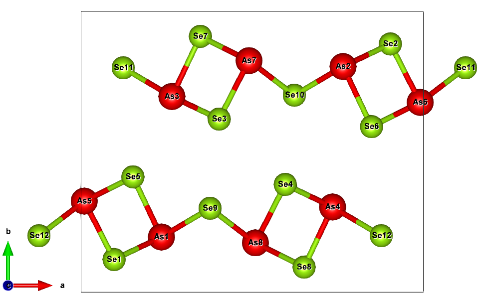
Figure 1: Crystalline structure of As₂Se₃. As atoms depicted in green and Se atoms shown in red.

The measurements of electrical conductivity Wood and Owen (1976); Marshall (1977); Brunst and Weiser (1985) exhibit an Arrhenius behavior, indicating that carrier transport is a thermally activated process. The activation energies obtained from the experimental results are similar, however, the measured values of the electrical conductivity showed large variation among the experiments. The measured Seebeck coefficient Brunst and Weiser (1985) is negative, indicating that electrons are responsible for electrical transport. These results suggest that trapped electrons in mid-gap levels created by defects are involved in the electrical transport. It has been suggested that antisite defects, i.e., threefold coordinated Se⁺ ions at As sites and twofold coordinated As^- ions at Se sites, are the defects that create such mid-gap levels. It has been argued that these defects have lower formation energies than vacancies and interstitials, since no bond breaking occurs upon their formation Tarnow et al. (1989). These defects can be thermally created, that means that, even under strict stoichiometric conditions, at finite temperature there would be an equilibrium concentration of these defects, which are created in pairs. However, deviations from stoichiometric conditions can also create such defects. Another feature of the material caused by these defects is the pinning of the Fermi level Brunst and Weiser (1985). All the experiments show a typical Arrhenius behavior, i.e., a linear increase of the logarithm of the electrical conductivity with the inverse of temperature, strongly suggesting that electron scattering by ionized defects dominates transport relaxation time and electron-phonon scattering is irrelevant.

The ultralow lattice thermal conductivity of As₂Se₃ renders it a prospective material for thermoelectric applications, however, several questions should be addressed before it can be considered a promising candidate. The goal of this work is to shed light on some of these questions. For instance, what are the concentrations of antisite defects in the samples studied in the experiments? Are these equilibrium concentrations? If defect concentration could be reduced, thus, depinning the Fermi level, what would be the thermoelectric transport properties of the material?

The approach used is a combination of first-principles calculations with the semiclassical Boltzmann transport equation (BTE) within the relaxation time approximation (RTA). This methodology has proven to be effective because it goes beyond parabolic or Kane models, and includes non-parabolicity, multiplicity and degeneracy of the band edges on the same footing Chaves et al. (2021).

II Methodology

II.0.1 Theoretical Approach to the Transport Properties

The transport properties of charge carriers in the diffusive regime are determined by solving numerically the semiclassical BTE for the nonequilibrium carrier distribution function $f_{n,{\bf{k}}}=f(\epsilon_{n,{\bf{k}}})$,

$$\frac{\partial f_{n,{\bf{k}}}}{\partial t}+{\bf{v}}_{n,{\bf{k}}}\cdot\nabla_{{\bf{r}}}f_{n,{\bf{k}}}-\frac{{\bf{F}}}{\hbar}\cdot\nabla_{{\bf{k}}}f_{n,{\bf{k}}}=\left(\frac{\partial f_{n,{\bf{k}}}}{\partial t}\right)_{coll}\leavevmode\nobreak\ ,$$ (2)

in which, $n$ and ${\bf{k}}$ are the band index and the wavevector, respectively. The carrier band velocity in the $\{n,{\bf{k}}\}$ state with energy $\epsilon_{n,{\bf{k}}}$ is given by ${\bf{v}}_{n,{\bf{k}}}=1/{\hbar}\nabla_{{\bf{k}}}\epsilon_{n,{\bf{k}}}$, and ${\bf{F}}$ is the Lorentz force acting upon the carriers. The right-hand side of the equation describes the charge carrier collisions involved in the various scattering processes that drive the system toward a steady state. The result of these scattering processes can be expressed by the per-unit-time transition probability, $W(n,{\bf{k}}|j,{\bf{{k}^{\prime}}})$, of a carrier starting at the state $\{n,{\bf{k}}\}$ and ending at state $\{j,{\bf{{k}^{\prime}}}\}$. If a steady state is to be reached, the principle of detailed balance should apply, thus the number of charge carriers reaching state $\{j,{\bf{{k}^{\prime}}}\}$ from $\{n,{\bf{k}}\}$ should be the same as the number departing state $\{j,{\bf{{k}^{\prime}}}\}$ toward state $\{n,{\bf{k}}\}$, in such a way that

$$\left(\frac{\partial f_{n,{\bf{k}}}}{\partial t}\right)_{coll}=\sum_{j,{\bf{{k}^{\prime}}}}[W(j,{\bf{{k}^{\prime}}}|n,{\bf{k}})f_{j,{\bf{{k}^{\prime}}}}\left(1-f_{n,{\bf{k}}}\right)\\ -W(n,{\bf{k}}|j,{\bf{{k}^{\prime}}})f_{n,{\bf{k}}}\left(1-f_{j,{\bf{{k}^{\prime}}}}\right)]\leavevmode\nobreak\ .$$ (3)

Once $f_{n,{\bf{k}}}$ is computed, all the transport properties can be readily evaluated.

If the system is sufficiently close to equilibrium, the nonequilibrium distribution function, $f_{n,{\bf{k}}}$, differs only slightly from that of the equilibrium state, $f_{n,{\bf{k}}}^{(0)}$, in such a way that $\Delta f(n,{\bf{k}})=\lvert{f_{n,{\bf{k}}}-f_{n,{\bf{k}}}^{(0)}}\lvert<<f_{n,{\bf{k}}}^{(0)}$. In this case, Eq. (3) can be written within the so-called RTA

$$\left(\frac{\partial f_{n,{\bf{k}}}}{\partial t}\right)_{coll}=-\frac{\Delta f(n,{\bf{k}})}{\tau_{n,{\bf{k}}}}\leavevmode\nobreak\ ,$$ (4)

where

$$\frac{1}{{\tau_{n,{\bf{k}}}}}=\sum_{{\bf{{k}^{\prime}}}}\sum_{j}W(n,{\bf{k}}|j,{\bf{{k}^{\prime}}})\\ \left(\frac{1-f^{(0)}_{j,{\bf{{k}^{\prime}}}}}{1-f^{(0)}_{n,{\bf{k}}}}-\frac{f^{(0)}_{n,{\bf{k}}}}{f^{(0)}_{j,{\bf{{k}^{\prime}}}}}\frac{\Delta f(j,{\bf{{k}^{\prime}}})}{\Delta f(n,{\bf{k}})}\right)\leavevmode\nobreak\ ,$$ (5)

in the case where quantum effects can be neglected, $W(n,{\bf{k}}|j,{\bf{{k}^{\prime}}})$ is independent of the magnetic field, ${\bf{B}}$ Askerov and Figarova (2010). Also, one can reasonably consider that $W(n,{\bf{k}}|j,{\bf{{k}^{\prime}}})$ does not depend on the electric field, ${\bf{E}}$, and the temperature gradient, $\nabla T$. As a result, for a homogeneous system, in zero magnetic field, and a time-independent electric field, in the steady-state regime, Eq. (2) becomes

$${\bf{v}}_{n,{\bf{k}}}\cdot\nabla_{{\bf{r}}}f_{n,{\bf{k}}}-\frac{e{\bf{E}}}{\hbar}\cdot\nabla_{{\bf{k}}}f_{n,{\bf{k}}}=-\frac{\Delta f(n,{\bf{k}})}{\tau_{n,{\bf{k}}}}\leavevmode\nobreak\ ,$$ (6)

from which it is possible to determine the nonequilibrium distribution function, as long as $\tau_{n,{\bf{k}}}$ does not depend on ${\bf{E}}$ or $\nabla T$.

Moreover, since we regard the deviation from equilibrium to be small, one can expand $f_{n,{\bf{k}}}$ to first order as

$$f_{n,{\bf{k}}}=f_{n,{\bf{k}}}^{(0)}-{\tau}_{n,{\bf{k}}}{\bf{v}}_{n,{\bf{k}}}\cdot{\bf{\Phi_{0}}}(\epsilon)\left(\frac{\partial f^{(0)}}{\partial\epsilon}\right)\leavevmode\nobreak\ ,$$ (7)

in which ${\bf{\Phi_{0}}}(\epsilon)=-e{\bf{E^{\prime}}}-\frac{\epsilon-\mu}{T}\nabla T$ is the generalized disturbing force (dynamic and static) driving the system out equilibrium, where ${\bf{E^{\prime}}}={\bf{E}}+(1/e)\nabla\mu=-\nabla(\phi_{0}-(\mu/e))$ is the gradient of the electrochemical potential. Using Eqs. (7) and (5), one obtains

$$\frac{1}{\tau_{n,{\bf{k}}}}=\sum_{{\bf{{k}^{\prime}}}}\sum_{j}W(n,{\bf{k}}|j,{\bf{{k}^{\prime}}})\\ \frac{1-f^{(0)}(\epsilon^{\prime})}{1-f^{(0)}(\epsilon)}\left(1-\frac{{\tau}_{j,{\bf{{k}^{\prime}}}}}{\tau_{n,{\bf{k}}}}\frac{{\bf{v}}_{j,{\bf{{k}^{\prime}}}}\cdot\bf{\Phi_{0}}(\epsilon^{\prime})}{{\bf{v}}_{n,{\bf{k}}}\cdot\bf{\Phi_{0}}(\epsilon)}\right)\leavevmode\nobreak\ .$$ (8)

If one considers that the per-unit-time probability of charge carrier transition, $W(n,{\bf{k}}|j,{\bf{{k}^{\prime}}})$, is a function only of the magnitudes of the vectors, $\lvert{\bf{k}}\lvert$ and $\lvert{\bf{{k}^{\prime}}}\lvert$, and the angle between them, ${\bf{k}}\cdot{\bf{{k}^{\prime}}}$, i.e., $W(n,{\bf{k}}|j,{\bf{{k}^{\prime}}})=W_{n,j}(\lvert{\bf{k}}\lvert,\lvert{\bf{{k}^{\prime}}}\lvert,{\bf{k}}\cdot{\bf{{k}^{\prime}}})$. Furthermore, regarding the dispersion relation as an arbitrary spherically symmetric function of the magnitude of the wavevector, $k=\lvert{\bf{k}}\lvert$,(not necessarily a parabolic function) and also that the charge carriers scattering is purely elastic, that is, with $\epsilon(\lvert{\bf{k}}\lvert)=\epsilon(\lvert{\bf{{k}^{\prime}}}\lvert)$ and consequently$\lvert{\bf{k}}\lvert=\lvert{\bf{{k}^{\prime}}}\lvert$, Eq. (8) may be further simplified as Askerov and Figarova (2010)

$$\frac{1}{{\tau_{n,{k}}}}=\sum_{{\bf{{k}^{\prime}}}}\sum_{j}W(n,{\bf{k}}|j,{\bf{{k}^{\prime}}})\left(1-\frac{{\bf{k}}\cdot{\bf{{k}^{\prime}}}}{k^{2}}\right)\leavevmode\nobreak\ .$$ (9)

Here, some comments are in order. Although Eq. (9) has been derived for isotropic bands, results obtained from it have been used to investigate transport properties of lead chalcogenides, which are anisotropic materials Ahmad and Mahanti (2010); Ravich et al. (1971). The usage of this methodology in this situation is possible due to the fact that, although anisotropic, the transport properties in these materials along the different directions are mutually independent, except for the case of magnetoresistance, which essentially depends on the anisotropy of the material. This methodology was applied in the case of SnSe yielding results in good agreement with the experiment for different values of temperature and chemical potential Chaves et al. (2021).

One can now compute the charge carrier current density

$${\bf{j}}=-\frac{2e}{V}\sum_{n}\sum_{k}{\bf{v}}_{n,{\bf{k}}}f_{n,{\bf{k}}}=-\frac{2e}{(2\pi)^{3}}\sum_{n}\int{{\bf{v}}_{n,{\bf{k}}}f_{n,{\bf{k}}}d{\bf{k}}}\leavevmode\nobreak\ ,$$ (10)

and the heat energy flux density

$${\bf{j}}_{Q}=\frac{2}{V}\sum_{n}\sum_{{\bf{k}}}\left(\epsilon_{n,{\bf{k}}}-\mu\right){\bf{v}}_{n,{\bf{k}}}f_{n,{\bf{k}}}\\ =\frac{2}{(2\pi)^{3}}\sum_{n}\int{\left(\epsilon_{n,{\bf{k}}}-\mu\right){\bf{v}}_{n,{\bf{k}}}f_{n,{\bf{k}}}d{\bf{k}}}\leavevmode\nobreak\ ,$$ (11)

where the factor $2$ is due to the electron spin, $e$ stands for the electron charge, $V$ is the crystal’s volume, and $\mu$ is the chemical potential.

Thermoelectric effects in anisotropic materials can be more conveniently studied using the tensorial formalism. The derivation of the off-diagonal coupling between the electronic current density, ${\bf{j}}$, and heat energy flux density, ${\bf{j}}_{Q}$, can be done in a more general way using the linear response theory Callen (1985) as

$$\begin{bmatrix}{\bf{j}}\\ {\bf{j}}_{Q}\end{bmatrix}=\begin{bmatrix}{\bf{L^{11}}}&{\bf{L^{12}}}\\ {\bf{L^{21}}}&{\bf{L^{22}}}\end{bmatrix}\cdot\begin{bmatrix}{\bf{E^{\prime}}}\\ -\frac{\nabla T}{T}\end{bmatrix}$$ (12)

where, ${\bf{L^{11}}}$, ${\bf{L^{12}}}$, ${\bf{L^{21}}}$, ${\bf{L^{22}}}$ are the moments of the generalized transport coefficients, which are called kinetic coefficient tensors, with ${\bf{L^{12}}}={\bf{L^{21}}}$ according to the Onsager reciprocity relations Callen (1985). These kinetic coefficients can be written as

$$\Lambda^{(\alpha)}(\mu;T)=e{{}^{2}}\int\Xi(\epsilon,\mu,T)(\epsilon-\mu)^{\alpha}\left(-\frac{\partial f^{(0)}(\mu;\epsilon,T)}{\partial\epsilon}\right)d\epsilon\leavevmode\nobreak\ ,$$ (13)

with ${\bf{L^{11}}}=\Lambda^{(0)}$, ${\bf{L^{21}}}={\bf{L^{12}}}=-(1/e)\Lambda^{(1)}$, and ${\bf{L^{22}}}=(1/e^{2})\Lambda^{(2)}$, in which $\Xi(\epsilon,\mu,T)$ is the transport distribution kernel (TDK) given by

$$\Xi(\epsilon,\mu,T)=\int\sum_{n}{{\bf{v}}_{n,{\bf{k}}}\otimes{\bf{v}}_{n,{\bf{k}}}{\tau}_{n,{k}}}(\mu,T)\delta(\epsilon-\epsilon_{n,{\bf{k}}})\frac{d{\bf{k}}}{8\pi^{3}}\leavevmode\nobreak\ .$$ (14)

Under the experimental condition of zero temperature gradient ($\nabla T=0$), the electrical conductivity tensor can be written as, $\sigma=\Lambda^{(0)}$, and under the experimental zero electric current condition, the Seebeck coefficient tensor is given by, $S=(eT)^{-1}\Lambda^{(1)}(\Lambda^{(0)})^{-1}$, while the charge carrier contribution to the thermal conductivity tensor can be identified as, $\kappa_{e}=(e^{2}T)^{-1}\left({\Lambda^{(1)}\cdot(\Lambda^{(0)})^{-1}}\cdot{\Lambda^{(1)}}-\Lambda^{(2)}\right)$.

Now we turn to the calculation of the per-unit-time transition probability. The so-called Born approximation in scattering theory considers that the magnitude of the Hamiltonian for charge carrier interaction, $H^{\prime}$ deviates only slightly from the magnitude of the non-perturbed Hamiltonian, $H$, that is, $H^{\prime}-H<<H$. In this case, the transition probability per-unit-time between Bloch states $\Psi_{j,{\bf{{k}^{\prime}}}}$ and $\Psi_{n,{\bf{k}}}$ can be well described by the first order perturbation theory (Fermi’s golden rule)

$$W(n,{\bf{k}}|j,{\bf{{k}^{\prime}}})=\frac{2\pi}{\hbar}\lvert\langle\Psi_{j,{\bf{{k}^{\prime}}}}\lvert{H^{\prime}}\lvert\Psi_{n,{\bf{k}}}\rangle\lvert^{2}\delta(\epsilon_{j,{\bf{{k}^{\prime}}}}-\epsilon_{n,{\bf{k}}})\leavevmode\nobreak\ .$$ (15)

The assumption is valid in the so-called weak coupling regime Hameau et al. (1999). The total scattering rate is obtained by integrating out such probability over the Brillouin zone (BZ). By using Eqs. (15) and (9), the expressions for the RTs associated with the different scattering mechanisms can be derived following Refs. Chaves et al. (2021) and Askerov and Figarova (2010). From the previous analysis of the experimental results, here we are concerned only with the scattering by ionized defects.

In particular, we consider only the concentration of ionized defects because the amount of charged donors or acceptors is usually considerably larger than that of neutral imperfections. The scattering of carriers by ionized defect (impurity) has been studied theoretically by Brooks and Herring (B-H) Brooks (1955); Chattipadhyay and Queisser (1981), by considering a screened Coulomb potential, the Born approximation to calculate the transition probabilities, and neglecting the perturbation effects of the defects on the electron energy levels and wave functions. In the B-H approach, it is assumed that the carriers are scattered by dilute concentrations of ionized defects randomly distributed throughout the semiconductor. It describes the scattering by charged defects without taking into account more complex effects, such as contributions from coherent scattering by pairs of ionized defects, which requires a quantum transport theory Moore (1967).

One can write the per-unit-time transition probability for the scattering of charge carriers by ionized defects in the plane-wave approximation as

$$W({\bf{k}}|{\bf{{k}^{\prime}}})=\frac{2\pi}{\hbar}\frac{N_{i}}{V}\\ \left|{\int U({\bf{r}})exp\left[i({\bf{k}}-{\bf{{k}^{\prime}}})\cdot{\bf{r}}\right]d{\bf{r}}}\right|^{2}\delta(\epsilon_{{\bf{{k}^{\prime}}}}-\epsilon_{{\bf{k}}})\leavevmode\nobreak\ ,$$ (16)

where $U({\bf{r}})$ is the scattering potential and $N_{i}$ is the ionized impurity concentration.

The long-range Coulomb potential energy, $U(\mbox{\boldmath{$r$}})=e\phi(r)=\pm e^{2}/\zeta_{0}r$, where $\phi$ is the potential at a point $r$ in the crystal, is due to the presence of positive (donor) or negative (acceptor) ionized defects and $\zeta_{0}$ is the static dielectric constant . The direct application of this potential in Eq. (16) leads to a logarithmic divergence, and therefore, a screened Coulomb potential has to be taken into account. According to the B-H approach, the potential can be written in a more rigorous form as $\phi(r)=\pm e/{\zeta{{}_{0}}r}\left(exp\left(-{r}/{r_{0}}\right)\right)$, where $r_{0}$ is the radius of ion field screening given by the following equation Askerov and Figarova (2010),

$$r_{0}^{-2}(n,k)=\frac{4\pi{e^{2}}}{\zeta_{0}}\int{-\frac{\partial f^{(0)}(\epsilon,\mu,T)}{\partial\epsilon_{n,k}}}g(\epsilon)d\epsilon\leavevmode\nobreak\ ,$$ (17)

where $g(\epsilon)$ is the density of states, which in the calculations is obtained numerically on an energy grid with spacing $d\epsilon$ sampled over $N_{k}$ ${\bf{k}}$-points

$$g(\epsilon)=\int\sum_{n}\delta(\epsilon-\epsilon_{n,{\bf{k}}})\frac{d{\bf{k}}}{8\pi^{3}}=\frac{1}{\Omega N_{k}}\sum_{n,{\bf{k}}}\frac{\delta(\epsilon-\epsilon_{n,{\bf{k}}})}{d\epsilon}\leavevmode\nobreak\ .$$ (18)

From Eqs. (9), (15), and (16), the RT for the scattering of charge carriers by ionized defects can be written for each band $n$ as

$$\tau_{def}(n,k)=\frac{\hbar\zeta{{}_{0}}{{}^{2}}}{2{\pi}{e^{4}}{N_{i}}F_{def}(k)}k^{2}\left|\frac{\partial\epsilon_{n,k}}{\partial k}\right|$$ (19)

where

$$F_{def}(k)=ln(1+\eta)-\frac{\eta}{1+\eta}\leavevmode\nobreak\ ,$$ (20)

is the screening function, with $\eta=(2kr_{0})^{2}$.

Since crystalline As₂Se₃ is anisotropic, Eqs. (17) and (19) should be considered for each crystalline direction separately, according to Eqs. 21 and 22 in Ref. 13. From the direction dependent relaxation times, one can obtain the corresponding TDKs and from them the direction dependent transport coefficient tensors can be determined.

The calculation of carrier transport properties were carried out using an in-house modified version of the BoltzTraP code Madsen and Singh (2006). The BoltzTraP code solves the linearized BTE using a Fourier interpolation of the band structure computed within the density functional theory (DFT) framework. The code computes all the integrals required to calculate the thermoelectric transport properties.

II.0.2 DFT Calculation of Crystalline Structure and Band Structure

Crystalline structure optimization and band structure calculations were performed using DFT within the generalized gradient approximation (GGA) using the formulation of Perdew-Burke-Ernzerhof (PBE) Perdew et al. (1996), as implemented in the VASP package Kresse and Hafner (1993); Kresse and Furthmüller (1996). To model the ion cores, projector augmented-wave (PAW) pseudopotentials Kresse and Joubert (1999) were used. The electronic wave functions were expanded in a plane-wave basis-set with a kinetic-energy cutoff of $700$ eV. To sample the BZ, a 5 x 7 x 15 Monkhorst-Pack ${\bf{k}}$-point mesh was used for the force on the ions calculations. Subsequently, to determine the transport properties, we used a finer ${\bf{k}}$-mesh of 15 x 19 x 45, which ensures the calculated transport coefficients to be converged. Within BoltzTraP the original ${\bf{k}}$-mesh is then interpolated onto a mesh five times as dense ($M/N_{KS}=5$). We used experimental structure Stergiou and Rentzeperis (1985) as starting configuration and relaxed the lattice parameters and atomic positions until all atomic force components were smaller than $1.0\text{\times}{10}^{-5}$ eV/$\AA$.

The weak interactions between layers along the $b$ direction were accurately described by incorporating van der Waals (vdW) corrections to DFT, according to the D3 approach as given by Grimme et al. Grimme et al. (2010). We found that DFT-D3 performed reasonably well in predicting both the lattice parameters and the internal atomic positions of As₂Se₃. We found that $a=12.216\>\AA$, $b=10.039\>\AA$ and $c=4.259\>\AA$, deviating by $1.1$%, $1.3$% and $0.58$%, respectively, from the experimental lattice parameters Stergiou and Rentzeperis (1985). In particular, the calculated angle between the a- and c-axes is 90.526$\degree$, which in very good agreement with the experiment, 90.458$\degree$ Stergiou and Rentzeperis (1985).

Our calculations indicate that the material has an indirect band gap of $1.21$ eV, which is in agreement with previous calculations Antonelli et al. (1986). It is well known that DFT calculations underestimates the band gap when compared with the experimental one, which in this case is $2.0$ eV Althaus and Weiser (1980). In our calculations of the thermoelectric transport properties, the experimental band gap is used. As it is usually done, this is accomplished by shifting upward rigidly the calculated conduction bands Chen et al. (2016); Li et al. (2019).

II.0.3 Energetics and Concentration of Defects

In order to estimate the equilibrium concentration of antisites in As₂Se₃, we first proceed to determine the formation energy of a single antisite defect, i.e., an As atom at a Se site and a Se atom at an As site, through total energy calculations. A pair of atoms is placed at the swapped positions as far as possible from each other inside the supercell. Since the number of atoms of each species remains the same upon the formation of the defect, the formation energy of a single antisite is calculated by simply taking the difference between the total energy of a supercell containing a defect and the total energy of a supercell of a perfect crystal. We obtained a formation energy, $\varepsilon_{def}$, for an antisite of 1.91 eV, which is in very good agreement with previous total energy calculations that yielded 1.88 eV Tarnow et al. (1989).

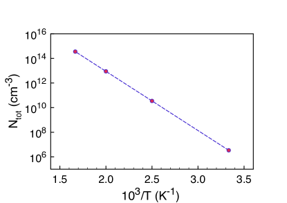
Figure 2: Equilibrium concentration of charged defects as a function of inverse temperature. The symbols correspond to results at 300 K, 400 K, 500 K, and 600 K, respectively.

The estimation of the equilibrium concentration of antisites requires a more elaborate calculation, which will be summarized as follows. First, we have to compute the number of ways, $\Omega_{def}$, one can form N_def pairs of atoms if there are N_As arsenic atoms and N_Se selenium atoms per unit of volume. The total number of pairs As-Se that can be formed is given by the product of the number of ways, $\Omega_{As}$, one can pick N_def arsenic atoms among N_As atoms and the number of ways, $\Omega_{Se}$, one can pick N_def selenium atoms among N_Se atoms, $\Omega_{def}=\Omega_{As}\cdot\Omega_{Se}$. This result stems from the fact that the order in which the atoms are swapped is irrelevant, since atoms of the same species are indistinguishable. From $\Omega_{def}$, one can calculate the configurational entropy of the system, $S_{conf}=k_{B}ln(\Omega_{def})$. Assuming that N_def $\ll$ N_As and N_def $\ll$ N_Se one can consider that the change in the vibrational entropy upon the formation of the defects is negligible. Thus, the configurational entropy accounts for the whole change in the entropy of the crystal due to the formation of the defects. Note that here we are taking the perfect crystal as the reference for both internal energy and entropy. Neglecting changes in the volume, one can write from the first law of thermodynamics

$$\frac{1}{T}=\frac{\partial S}{\partial E},$$ (21)

where $E=N_{def}\varepsilon_{def}$. Therefore, we have

$$\frac{1}{T}=\frac{k_{B}}{\varepsilon_{def}}\frac{\partial ln(\Omega_{def})}{\partial N_{def}}.$$ (22)

From Eq. 22, one can obtain the equilibrium concentration of antisite defects

$$N_{def}^{eq}=(N_{As}N_{Se})^{1/2}e^{-\frac{\varepsilon_{def}}{2k_{B}T}}.$$ (23)

Therefore, the total concentration of charged defects in equilibrium ($As^{+}$ and $Se^{-}$) is given by $N_{tot}=2N_{def}^{eq}$. To our knowledge, Eq. 23 has previously appeared in Ref. 9, however, details of its derivation cannot be found, either there or elsewhere.

The concentrations, $N_{As}=1.53\times 10^{-22}$ cm^-3 and $N_{Se}=2,30\times 10^{-22}$ cm^-3 are obtained considering that in the 20-atom unit cell, whose volume is 5.22 $\times 10^{-22}$ cm^-3, there are 8 As atoms and 12 Se atoms. Fig. 2 depicts the results from Eq. 23 in the temperature range from 300 K to 600 K. Due to the relatively large formation energy, the equilibrium concentration of charged defects is low, of the order of 10¹⁴ cm^-3 at 600 K.

III Results and Discussion

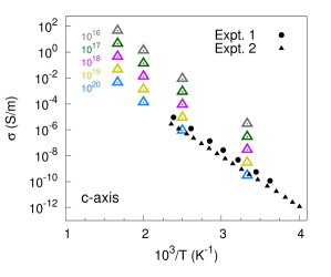
Figure 3: Electrical conductivity as a function of inverse temperature for defects concentrations ranging from 10¹⁶cm^-3 to 10²⁰cm^-3. Experimental results from two different samples are from Ref. 9.

In order to determine the thermoelectric transport properties, two quantities should be specified beforehand, namely, the chemical potential or Fermi level and the concentration of charged defects. For the former, we used the experimental chemical potential provided in Ref. 9. Regarding the latter, we performed calculations for different values of the concentration of ionized defects. Our results for the electrical conductivity as a function of temperature, together with experimental ones from Ref. 9, are shown in Fig. 3. Our findings indicate good agreement with the experimental results for concentrations between 10¹⁹ cm^-3 and 10²⁰ cm^-3 .

Next, we compare these results with those for the equilibrium concentration of charged defects determined using Eq. 23. As it has been previously pointed out, even at the temperature of 600 K, the equilibrium concentration of charged defects is of only 3.6 $\times$ $10^{14}$ cm^-3, which is orders of magnitude smaller than that yielded by conductivity calculations. This large discrepancy strongly suggests that the large concentration of defects in the samples investigated experimentally is out-of-equilibrium, possibly formed during crystal growth due to kinetic factors and/or deviations from stoichiometry. A similar out-of-equilibrium concentration of defects has been proposed by Zhou et al. Zhou et al. (2018) to explain the high carrier density in SnSe. This last result is quite interesting, because it indicates that, in principle, there is plenty of room for the reduction of the concentration of antisite defects in the material. That could lead to Fermi level depinning and allow to utilize the material in thermoelectric applications.

In Fig. 4 we show the results for the Seebeck coefficient calculated assuming the concentration of charged defects of $10^{20}$ cm^-3. In this case also, we can see a good agreement between our results and those from Ref. 9.

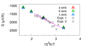
Figure 4: Seebeck coefficient as a function of inverse temperature for defect concentration of 10²⁰cm^-3. Experimental results from two different samples are from Ref. 9.

Let us now assume that the concentration of defects can be reduced and consequently Fermi level depinning can be achieved, what thermolectric properties the material would exhibit? Aside from the ability to dope the material, which would provide relevant increase in the carrier density, the reduction in charged defects concentration would decrease substantially scattering rates. Our calculations indicate that at the highest temperature considered of 600 K, if the concentration of charged defects could be decreased from $\sim$ 10²⁰ cm^-3 to $\sim$ 10¹⁷ cm^-3, the carrier relaxation time along the c-direction due to scattering by defects would increase from a value $\sim$ 0.01 fs to $\sim$ 10 fs. These values are similar to relaxation times found in materials such as SnSe Chaves et al. (2021). Since a full first-principles calculations of the carrier-phonon scattering is beyond the scope of this work, because of the large size of the unit cell, we adopt the approximation that the full scattering relaxation time is independent of the wavevector, $\bf{k}$, of the charge carrier. In this case, the relaxation time, $\tau_{n,k}(\mu,T)=\tau(\mu,T)$, can be taken out of the integral in $d\bf{k}$ in Eq. 14 in the calculation of the TDKs. In order to check the validity of this approximation, we utilize the following procedure, since in the formula to compute the Seebeck coefficient the relaxation time cancels out, we are able to vary the chemical potential in order to adjust the Seebeck coefficient to the experimental value Brunst and Weiser (1985) for a set of values of $T$. Our results for the chemical potential obtained from this procedure are in good agreement with the experimental findings from Ref. 9 indicating that indeed the approximation is reliable in this case.

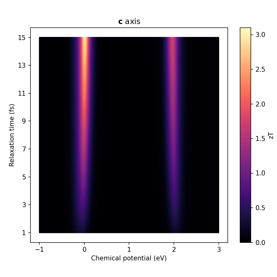
Figure 5: Figure of merit of As₂Se₂ as a function of the Fermi level and relaxation time.

Fig. 5 displays the figure of merit $zT$ along the c-axis as a function of the chemical potential and relaxation time. The thermal conductivity used in the calculations is given by the sum of two contributions from carriers and from phonons. For the latter contribution, we employed that obtained in Ref. 4. For the p-type material, $zT$ can reach the high value of 3, while for the n-type case $zT$ is about 2, in both cases for relaxation times above 10 fs.

It should be emphasized that the calculations in Ref. 4 considered only the perfect crystal case. The inclusion of the effect of defects would further decrease the lattice contribution to the thermal conductivity, therefore, increasing $zT$.

III.1 Summary

Based on the solution of the linearized BTE within the RTA and using smooth Fourier interpolation of the KS eigenvalues and their corresponding velocities, we calculated the thermoelectric transport properties of As₂Se₃. The calculations were done using a methodology that incorporates anisotropy in the determination of the RTs Chaves et al. (2021). Comparison of our results with experimental findings Brunst and Weiser (1985) indicate that scattering by charged defects dominates the relaxation processes in this compound. According to our calculations, the concentration of charged defects is about 10¹⁹ cm^-3. Previous DFT-based calculations Tarnow et al. (1989) indicate that antisites, are such defects, namely, threefold coordinated Se⁺ ions at As sites and twofold coordinated As^- ions at Se sites. We have also estimated the equilibrium concentration of these defects, which, due to their relatively high formation energy, is of only 10¹⁴ cm^-3 at the highest temperature considered of 600 K. These results suggest that the large concentration of defects in the samples investigated experimentally is the result of kinetic factors and/or deviations from stoichiometry. Therefore, at least in principle, there are no fundamental reasons to prevent a reduction of the charged defects. Based on this conclusion, we computed the thermoelectric transport properties assuming that the concentration of charged defects could be reduced, which would increase the RTs to values similar to those found in other chalcogenide compounds such as SnSe Chaves et al. (2021). For relaxation times above 10 fs, we obtain for the p-type material $zT$ as high as 3, while for the n-type case $zT$ of about 2. Those remarkable values of $zT$ are somehow underestimated, since they were obtained using the phonon thermal conductivity previously calculated by Gonzalez-Romero et al. González-Romero et al. (2018), which did not consider phonon scattering by defects.

References

- Beretta et al. (2019) D. Beretta, N. Neophytou, J. M. Hodges, M. G. Kanatzidis, D. Narducci, M. Martin- Gonzalez, M. Beekman, B. Balke, G. Cerretti, W. Tremel, A. Zevalkink, A. I. Hofmann, C. Müller, B. Dörling, M. Campoy-Quiles, and M. Caironi, Materials Science and Engineering: R: Reports 138, 100501 (2019).
- Zhao et al. (2014) L.-D. Zhao, S.-H. Lo, Y. Zhang, H. Sun, G. Tan, C. Uher, C. Wolverton, V. P. Dravid, and M. G. Kanatzidis, Nature 508, 373 (2014).
- Jia et al. (2020) T. Jia, Z. Feng, S. Guo, X. Zhang, and Y. Zhang, ACS Applied Materials & Interfaces 12, 11852 (2020).
- González-Romero et al. (2018) R. L. González-Romero, A. Antonelli, A. S. Chaves, and J. J. Meléndez, Phys. Chem. Chem. Phys. 20, 1809 (2018).
- Nielsen et al. (2013) M. D. Nielsen, V. Ozolins, and J. P. Heremans, Energy Environ. Sci. 6, 570 (2013).
- Tanaka and Shimakawa (2021) K. Tanaka and K. Shimakawa, Amorphous Chalcogenide Semiconductors and Related Materials (Springer International Publishing, 2021).
- Wood and Owen (1976) C. Wood and A. Owen, Solid State Communications 20, 329 (1976).
- Marshall (1977) J. M. Marshall, Journal of Physics C: Solid State Physics 10, 1283 (1977).
- Brunst and Weiser (1985) G. Brunst and G. Weiser, Philosophical Magazine B 51, 67 (1985).
- Stergiou and Rentzeperis (1985) A. Stergiou and P. Rentzeperis, Zeitschrift für Kristallographie 173, 185 (1985).
- Althaus and Weiser (1980) H. L. Althaus and G. Weiser, physica status solidi (b) 99, 277 (1980).
- Tarnow et al. (1989) E. Tarnow, J. D. Joannopoulos, and M. C. Payne, Phys. Rev. B 39, 6017 (1989).
- Chaves et al. (2021) A. S. Chaves, R. L. González-Romero, J. J. Meléndez, and A. Antonelli, Phys. Chem. Chem. Phys. 23, 900 (2021).
- Askerov and Figarova (2010) B. Askerov and S. Figarova, Thermodynamics, Gibbs Method and Statistical Physics of Electron Gases (Springer-Verlag Berlin Heidelberg, 2010).
- Ahmad and Mahanti (2010) S. Ahmad and S. Mahanti, Phys. Rev. B 81, 165203 (2010).
- Ravich et al. (1971) Y. Ravich, B. Efimova, and V. Tamarchenko, Physica Status Solid B-Basic Solid State Physics 43, 11+ (1971).
- Callen (1985) H. Callen, Thermodynamics and an Introduction to Thermostatistics (Wiley, 1985).
- Hameau et al. (1999) S. Hameau, Y. Guldner, O. Verzelen, R. Ferreira, G. Bastard, J. Zeman, A. Lemaître, and J. M. Gérard, Phys. Rev. Lett. 83, 4152 (1999).
- Brooks (1955) H. Brooks, in Advances in electronics and electron physics, Vol. 7 (Elsevier, 1955) pp. 85–182.
- Chattipadhyay and Queisser (1981) D. Chattipadhyay and H. Queisser, Rev. Mod. Phys. 53, 745 (1981).
- Moore (1967) E. Moore, Physical Review 160, 607 (1967).
- Madsen and Singh (2006) G. K. Madsen and D. J. Singh, Computer Physics Communications 175, 67 (2006).
- Perdew et al. (1996) J. P. Perdew, K. Burke, and M. Ernzerhof, Physical Review Letters 77, 3865 (1996).
- Kresse and Hafner (1993) G. Kresse and J. Hafner, Phys. Rev. B 48, 13115 (1993).
- Kresse and Furthmüller (1996) G. Kresse and J. Furthmüller, Phys. Rev. B 54, 11169 (1996).
- Kresse and Joubert (1999) G. Kresse and D. Joubert, Phys. Rev. B 59, 1758 (1999).
- Grimme et al. (2010) S. Grimme, J. Antony, S. Ehrlich, and H. Krieg, The Journal of Chemical Physics 132, 154104 (2010).
- Antonelli et al. (1986) A. Antonelli, E. Tarnow, and J. D. Joannopoulos, Phys. Rev. B 33, 2968 (1986).
- Chen et al. (2016) W. Chen, J.-H. Pöhls, G. Hautier, D. Broberg, S. Bajaj, U. Aydemir, Z. M. Gibbs, H. Zhu, M. Asta, G. J. Snyder, B. Meredig, M. A. White, K. Persson, and A. Jain, J. Mater. Chem. C 4, 4414 (2016).
- Li et al. (2019) S. Li, Z. Tong, and H. Bao, J. Appl. Phys. 126, 025111 (2019).
- Zhou et al. (2018) Y. Zhou, W. Li, M. Wu, L.-D. Zhao, J. He, S.-H. Wei, and L. Huang, Phys. Rev. B 97, 245202 (2018).