Spin-flip scattering engendered negative $\Delta_{T}$ noise

Abstract

$\Delta_{T}$ noise generated due to temperature gradient in the absence of charge current has recently attracted a lot of interest. In this paper, for the first time, we derive spin-polarized charge $\Delta_{T}$ noise and spin $\Delta_{T}$ noise along with its shot noise-like and thermal noise-like contributions. Introducing a spin flipper at the interface of a bilayer metal junction with a temperature gradient, we examine the impact of spin-flip scattering. We do a detailed analysis of charge and spin $\Delta_{T}$ noise in four distinct setups for two distinct temperature regimes: the first case of one hot & the other cold reservoir and the second case of reservoirs with comparable temperatures, and also two distinct bias voltage regimes: the first case of zero bias voltage and second case of finite bias voltage. In all these regimes, we ensure that the net charge current transported is zero always. We find negative charge $\Delta_{T}$ noise for reservoirs at comparable temperatures while for the one hot & other cold reservoir case, charge $\Delta_{T}$ noise is positive. We also see that spin $\Delta_{T}$ noise and spin $\Delta_{T}$ thermal noise-like contributions are negative for one hot and other cold reservoir case. Recent work on the general bound for spin $\Delta_{T}$ shot noise with a spin-dependent bias suggests it is always positive. In this paper, we see spin $\Delta_{T}$ shot noise-like contribution to be negative in contrast to positive charge $\Delta_{T}$ shot noise contribution, although in absence of any spin dependent bias. Spin-flip scattering exhibits the intriguing effect of a change in sign in both charge and spin $\Delta_{T}$ noise, which can help probe spin-polarized transport.

I Introduction

Quantum noise [1] has been used to probe many facets of electron transport, like current-current correlations[2], fractional charges[3], wave-particle duality, etc. There are two distinctive contributions to electronic noise in mesoscopic devices: thermal noise and shot noise, which have distinct origins [4, 5]. At equilibrium, the temporal current fluctuations due to the thermal agitation of electrons is referred to as thermal noise, also known as Johnson-Nyquist noise [6]. Thermal noise vanishes at zero temperature and is related to the conductance of the system. The non-equilibrium temporal current fluctuations lead to shot noise which exists even at zero temperature. Shot noise arises due to the discreteness of the particles and can be used as an entanglement detector [7], and also to probe wave-particle duality [1, 8]. Shot noise is crucial in providing more detailed information on quantum transport compared to the conductance [6]. Recently, $\Delta_{T}$ noise, accompanied by zero charge current, has been experimentally measured [9, 10]. It arises due to a temperature gradient in non-equilibrium systems [11, 12, 13]. This intriguing noise, in a non-equilibrium situation, measured in recent experiments has generated much interest from both theoretical [11, 14, 12] and experimental perspectives. It has been observed across nanoscale conductors [13], in elementary quantum circuits [9], and metallic tunnel junctions [10]. General bounds for charge $\Delta_{T}$ noise have been found in Ref. [12]; which show that the shot noise-like contribution to charge $\Delta_{T}$ noise, i.e., $\Delta_{Tsh}$ is always less than thermal noise contribution to $\Delta_{T}$ noise, i.e., $\Delta_{Tth}$ or $\Delta_{Tsh}/\Delta_{Tth}<1$. This general bound holds for both charge $\Delta_{T}$ noise (charge current-current correlations in the absence of charge current) and spin $\Delta_{T}$ noise (spin current-current correlations in the absence of spin current)  [12, 15]. Finite $\Delta_{T}$ noise has been observed in a recent experiment with a metallic scale atomic junction at vanishing charge current [13]. Recent works have proposed that the sign of $\Delta_{Tsh}$ shot noise contribution can reveal quantum statistics, see Ref. [16]. $\Delta_{Tsh}$ shot noise contribution is always positive for fermions, whereas it can be positive or negative for bosons. However, the sign of equilibrium thermal noise has no dependence on quantum statistics [4].

In this paper, we study charge and spin $\Delta_{T}$ noise in the presence of spin-flip scattering. Spin-flip scattering occurs when an incident electron interacts with an interfacial spin flipper. Spin current is of great importance in spintronics, which motivates us to study both spin and charge $\Delta_{T}$ noise. We look at the effect of spin-flip scattering at vanishing charge current via charge $\Delta_{T}$ noise and at vanishing spin current via spin $\Delta_{T}$ noise along with their respective $\Delta_{T}$ shot noise-like contribution and $\Delta_{T}$ thermal noise-like contributions. Apart from a single work in a spin-biased setup [15], in which transmission is spin-independent, wherein spin $\Delta_{T}$ shot noise has been calculated, there is a complete absence of published works on spin $\Delta_{T}$ noise with spin-polarized transmission. We in this work are the first to calculate spin $\Delta_{T}$ noise for a junction with spin-polarized transmission, which includes thermal and shot noise-like contributions to spin $\Delta_{T}$ noise.

Further, for the first time, we provide a more general approach to the study of charge and spin $\Delta_{T}$ noise, with four distinct setups as depicted in subsectionsII.4 and II.5. These setups include the zero-bias case (setup 1), the finite-bias case (setup 2) for reservoirs with comparable temperatures. They also include the zero-bias case (setup 3) and the finite-bias case (setup 4) for one hot and other cold reservoir. Previously, there have been a few works on calculating $\Delta_{T}$ noise for some of these setups. Specifically, for setup 4 in [12] with two generic conductors, while for setups 1 and 4 in [14] with two normal metals separated by a quantum dot, and for setup 1 in [11]. In all these works, only charge $\Delta_{T}$ noise is calculated while spin-dependent transport is absent. One should note that for setups 2 and 3, no one has calculated charge $\Delta_{T}$ noise yet.

The main findings of this work are: we see that charge $\Delta_{T}$ noise is negative due to spin-flip scattering. We also calculate charge $\Delta_{T}$ noise in the absence of any spin-flip scattering, wherein it is always positive. Negative charge $\Delta_{T}$ noise arises due to the dominant thermal noise-like contribution, which is negative. As far as we know, negative charge $\Delta_{T}$ noise or negative charge $\Delta_{T}$ thermal noise contribution has not been seen in any system. However, negative charge $\Delta_{T}$ thermal noise-like contribution has been predicted in Ref. [14]. Negative charge $\Delta_{T}$ thermal noise-like contribution is related to negative differential charge conductance [14]. Further, we show that the negative charge $\Delta_{T}$ noise is a sign of spin-flip scattering due to temperature bias. $\Delta_{T}$ noise measurement is an adaptable probe to study transport in a system without any specific design limitations [13].

Further, in this work, we see that spin $\Delta_{T}$ shot noise-like contribution is always less than spin $\Delta_{T}$ thermal noise contribution [15] in the four setups. Notably, we also see that in our bilayer metallic junction with spin-flip scattering, both charge $\Delta_{T}$ noise and spin $\Delta_{T}$ noise obey this general bound, i.e., the magnitude of charge (spin) shot noise-like contribution is always less than charge (spin) thermal noise-like contribution to charge (spin) $\Delta_{T}$ noise. The sign of charge $\Delta_{T}$ shot noise depends on the tunneling process and its scaling dimension, with fermions exhibiting a positive sign and bosons showing either positive or negative signs [16, 11]. Moreover, we see in our setups that the spin $\Delta_{T}$ shot noise-like contribution can turn negative for reservoirs with comparable temperatures, unlike charge $\Delta_{T}$ shot noise-like contribution, which is always positive due to fermionic statistics [16]. Our work shows that a unique negative spin $\Delta_{T}$ shot noise-like contribution arises from spin-flip scattering, even for fermions.

The layout of the paper is as follows: in section II, we first discuss our chosen setup metal($N_{1}$)/spin-flipper(SF)/metal($N_{2}$) briefly, then in subsection II.1, we explain the phenomena of spin-flip scattering by introducing a spin-flipper in metal/metal interface, focusing on wave functions and boundary conditions. Subsequently, we discuss finite temperature charge and spin quantum noise followed by spin-polarized $\Delta_{T}$ noise for the different setups. In section III, we discuss charge and spin $\Delta_{T}$ noise and the ratio of $\Delta_{T}$ shot noise to $\Delta_{T}$ thermal noise contributions and investigate the impact of spin-flip scattering in a bilayer metallic junction. Next, in section IV, we analyze via a table the results for the charge as well as spin $\Delta_{T}$ noise and the respective general bounds for each setup. We also discuss $\Delta_{T}$ shot noise-like and $\Delta_{T}$ thermal noise-like contributions to charge and spin $\Delta_{T}$ noise, followed by experimental realization and the conclusions of our work in section V. In Appendix A, we derive in detail the thermovoltage for vanishing current for each setup, in Appendix B, we derive the expressions for spin-polarized quantum noise, and finally, in Appendix C, we derive expressions for $\Delta_{T}$ shot noise-like contribution followed by $\Delta_{T}$ thermal noise-like contribution to charge $\Delta_{T}$ noise and spin $\Delta_{T}$ noise for each setup.

II Theory

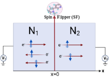
Figure 1: Illustration of the 1D bilayer metal junction, with a magnetic impurity (spin $S$) which acts as a spin-flipper at the interface $x=0$.

In Fig. 1, a 1D bilayer metal junction consisting of a spin magnetic impurity at the interface $x=0$ is shown. When a spin-up or spin-down electron from left normal metal $N_{1}$ is incident on the interfacial spin-flipper ($x=0$), there may be a mutual spin-flip, and the electron may be reflected to normal metal $N_{1}$ or transmitted to normal metal $N_{2}$ as a spin-down or spin-up electron. The Hamiltonian of our bilayer junction with a spin-flipper [17] at the interface is,

$$H=\frac{p^{2}}{2m^{*}}-H_{SF},$$ (1)

where $H_{SF}=J_{0}\delta(x)\vec{s}.\vec{S}$ with effective mass $m^{*}$ and $J_{0}$ being the relative strength of exchange interaction between electron spin $\vec{s}$ and magnetic impurity spin $\vec{S}$. To compare with the case of no spin-flip scattering, we replace the spin-flipper with a delta potential $\delta(x)$ at the interface $x=0$. The Hamiltonian $H_{SF}$ then becomes, $H_{SF}=H_{N}=J_{0}\delta(x)$. As expressed in the second term of Eq. (1), the effective Heisenberg interaction reduces the two-electron problem to a single-electron one. The exchange interaction is given as $\vec{s}.\vec{S}=s_{z}.S_{z}+\frac{1}{2}(s^{-}S^{+}+s^{+}S^{-})$, where $s^{\pm}=s_{x}\pm is_{y}$ and $S^{\pm}=S_{x}\pm iS_{y}$ are raising and lowering operators for electron’s spin and spin-flipper’s spin respectively. $s_{x},s_{y},s_{z}$, and $S_{x},S_{y},S_{z}$ are $x,y,z$ components of the electron’s spin operator and spin-flipper’s spin operator, respectively.

II.1 Spin-flip scattering

The wave functions in $N_{1}$ and $N_{2}$ region, for an electron with spin-up incident from $N_{1}$ can be written as in Fig. 1,

$$\psi_{N_{1}}(x) =\left(\begin{array}[]{c}1\\ 0\\ \end{array}\right)(e^{ikx}+r^{\uparrow\uparrow}e^{-ikx})\phi^{s}_{m}+r^{\uparrow\downarrow}\left(\begin{array}[]{c}0\\ 1\\ \end{array}\right)e^{-ikx}\phi^{s}_{m+1},\leavevmode\nobreak\ \text{for}\hskip 2.27626ptx<0,$$ (6)

$$\psi_{N_{2}}(x) =t^{\uparrow\uparrow}\left(\begin{array}[]{c}1\\ 0\end{array}\right)e^{ikx}\phi^{s}_{m}+t^{\uparrow\downarrow}\left(\begin{array}[]{c}0\\ 1\end{array}\right)e^{-ikx}\phi^{s}_{m+1},\leavevmode\nobreak\ \text{ for}\hskip 2.56064ptx>0,$$ (11)

where $\phi^{s}_{m}$ is the eigenfunction of $S_{z}$ such that $S_{z}\phi^{s}_{m}=m\phi^{s}_{m}$ with $m$ being spin magnetic moment and $k$ is electron wave vector with kinetic energy $E$, i.e., $k=\sqrt{2m^{*}E/\hbar^{2}}$ with energy of incident electron $E>0$. Reflection amplitudes for an incident spin-up electron to be reflected as the spin-up electron are denoted as $r^{\uparrow\uparrow}$ and to be reflected as the spin-down electron is denoted as $r^{\uparrow\downarrow}$. $t^{\uparrow\uparrow}$ is the transmission amplitude for the incident spin-up electron to be transmitted as spin-up, and $t^{\uparrow\downarrow}$ is for the incident spin-up electron to be transmitted as spin-down.

The electron spin and spin-flipper spin operators $\vec{s}$ and $\vec{S}$ operating on spinor for spin-up electron [17] and spin-flipper eigen function gives

$$\vec{s}.\vec{S}\left(\begin{array}[]{c}1\\ 0\\ \end{array}\right)\phi^{s}_{m}=\frac{m}{2}\left(\begin{array}[]{c}1\\ 0\\ \end{array}\right)\phi^{s}_{m}+\frac{\tau}{2}\left(\begin{array}[]{c}0\\ 1\\ \end{array}\right)\phi^{s}_{m+1}.$$ (18)

Similarly, $\vec{s}.\vec{S}$ acting on spinor for spin-down electron and spin-flipper eigen function gives

$$\vec{s}.\vec{S}\left(\begin{array}[]{c}0\\ 1\\ \end{array}\right)\phi^{s}_{m}=-\frac{m}{2}\left(\begin{array}[]{c}0\\ 1\\ \end{array}\right)\phi^{s}_{m}+\frac{\tau_{1}}{2}\left(\begin{array}[]{c}1\\ 0\\ \end{array}\right)\phi^{s}_{m-1},$$ (25)

where $\tau=\sqrt[]{(S-m)(S+m+1)}$, $\tau_{1}=\sqrt[]{(S+m)(S-m+1)}$ are spin-flip probabilities for up and down spin electron incident at left normal metal, with $S$ being the spin-flipper’s spin.

$$\begin{array}{cc}\hfill 1.{\uparrow }_{e^{-}}& \otimes {\Uparrow }_S\stackrel{S=m}{\to }\frac{m}{2}({\uparrow }_{e^{-}}\otimes {\Uparrow }_S)\hfill \\ \hfill 2.{\uparrow }_{e^{-}}& \otimes {\Downarrow }_S\stackrel{S\ne m}{\to }\frac{m}{2}({\uparrow }_{e^{-}}\otimes {\Downarrow }_S)+\frac{\tau }{2}({\downarrow }_{e^{-}}\otimes {\Uparrow }_S)\hfill \\ \hfill 3.{\downarrow }_{e^{-}}& \otimes {\Uparrow }_S\stackrel{S\ne -m}{\to }\frac{-m}{2}({\downarrow }_{e^{-}}\otimes {\Uparrow }_S)+\frac{{\tau }_1}{2}({\uparrow }_{e^{-}}\otimes {\Downarrow }_S)\hfill \\ \hfill 4.{\downarrow }_{e^{-}}& \otimes {\Downarrow }_S\stackrel{S=-m}{\to }\frac{-m}{2}({\downarrow }_{e^{-}}\otimes {\Downarrow }_S)\hfill \end{array}$$

Figure 2: Illustration of different spin configurations when spin $\uparrow$ or $\downarrow$ electron encounters a spin-flipper with $S=\pm m$ or $S\neq\pm m$. $\tau$ and $\tau_{1}$ are spin-flip probabilities for spin-up and spin-down incident electrons.

When the electron’s relaxation time is much greater than the spin-flipper’s relaxation time $\tau_{e}\gg\tau_{sf}$, the spin-flipper will flip back before encountering the next incident electron, see Fig. 2. Therefore spin magnetic moment $m$ for a specific spin-flipper’s spin $S$ is not fixed, and to calculate any transport quantity, the average over all possible $m$ values is taken. We consider the cases where a spin-up incident electron interacts in either spin-configuration 1 ($S=m$) or spin-configuration 2 ($S\neq m$). Likewise, for spin-down incident electron, the spin-flipper interacts via spin-configuration 3 ($S\neq-m$) or spin-configuration 4 ($S=-m$).

The boundary conditions at the interface $x=0$ are, see Fig 1,

$$\left.\psi_{N1}(x)\right|_{x=0} = \left.\psi_{N2}(x)\right|_{x=0},$$

$$\left.\frac{d\psi_{N2}}{dx}\right|_{x=0}-\left.\frac{d\psi_{N1}}{dx}\right|_{x=0} = \left.\frac{-2m^{*}J_{0}\delta(x)\vec{s}.\vec{S}}{\hbar^{2}}\psi_{N1}\right|_{x=0}.$$ (26)

Substituting Eq. (11) in Eq. (26) and using Eqs. (18) and (25), we get:

$$r^{\uparrow\uparrow}-t^{\uparrow\uparrow}=-1,\leavevmode\nobreak\ \leavevmode\nobreak\ \leavevmode\nobreak\ \leavevmode\nobreak\ \leavevmode\nobreak\ \leavevmode\nobreak\ r^{\uparrow\downarrow}-t^{\uparrow\downarrow}=0,$$

$$(1-iJm)r^{\uparrow\uparrow}-iJ\tau r^{\uparrow\downarrow}+t^{\uparrow\uparrow}=1+iJm,$$

$$-iJ\tau r^{\uparrow\uparrow}+(1+iJ(m+1))r^{\uparrow\downarrow}+t^{\uparrow\downarrow}=iJ\tau,$$ (27)

where the parameter $J$ is dimensionless, i.e., $J=\frac{m^{*}J_{0}}{\hbar^{2}k}$. This can also be expressed as $J=\frac{1}{\sqrt[]{\frac{E}{cJ_{0}^{2}}}}$, where $c=\frac{m^{*}}{2\hbar^{2}}$.

Solving Eq. (27), we get normal reflection amplitude for no-flip ($r^{\uparrow\uparrow}=s^{\uparrow\uparrow}_{11}$), normal reflection amplitude for spin-flip ($r^{\uparrow\downarrow}=s^{\uparrow\downarrow}_{11}$), transmission amplitude for no-flip ($t^{\uparrow\uparrow}=s^{\uparrow\uparrow}_{12}$) and transmission amplitude for spin-flip ($t^{\uparrow\downarrow}=s^{\uparrow\downarrow}_{12}$). The scattering amplitudes for a spin-up incident electron can be simplified as follows:

$$s^{\uparrow\uparrow}_{11} = \frac{\tau^{2}+m\left(1-2i\sqrt[]{\frac{E}{cJ^{2}_{0}}}+m\right)}{Dn},\leavevmode\nobreak\ \leavevmode\nobreak\ s^{\uparrow\downarrow}_{11}=\frac{2i\tau\sqrt[]{\frac{E}{cJ^{2}_{0}}}}{Dn},$$

$$s^{\uparrow\uparrow}_{12} = \frac{2i\sqrt[]{\frac{E}{cJ^{2}_{0}}}\left(1+m-2i\sqrt[]{\frac{E}{cJ^{2}_{0}}}\right)}{Dn},\leavevmode\nobreak\ \leavevmode\nobreak\ s^{\uparrow\downarrow}_{12}=\frac{2i\tau\sqrt[]{\frac{E}{cJ^{2}_{0}}}}{Dn},$$ (28)

where $Dn=4\frac{E}{cJ^{2}_{0}}+2i\sqrt[]{\frac{E}{cJ^{2}_{0}}}+\tau^{2}+m+m^{2}$. Reflection probabilities for spin-up incident electron for no-flip and spin-flip are $\mathcal{R}^{\uparrow\uparrow}=|r^{\uparrow\uparrow}|^{2}$ and $\mathcal{R}^{\uparrow\downarrow}=|r^{\uparrow\downarrow}|^{2}$. Transmission probabilities for spin-up incident electron for no-flip and spin-flip are $\mathcal{T}^{\uparrow\uparrow}=|t^{\uparrow\uparrow}|^{2}$ and $\mathcal{T}_{\uparrow\downarrow}=|t^{\uparrow\downarrow}|^{2}$. Similarly, the scattering amplitudes for a spin-down incident electron can be simplified as follows:

$$s^{\downarrow\downarrow}_{11} = \frac{\tau^{2}_{1}+m\left(-1+2i\sqrt[]{\frac{E}{cJ^{2}_{0}}}+m\right)}{Dn1},\leavevmode\nobreak\ \leavevmode\nobreak\ s^{\downarrow\uparrow}_{11}=\frac{2i\tau_{1}\sqrt[]{\frac{E}{cJ^{2}_{0}}}}{Dn1},$$

$$s^{\downarrow\downarrow}_{12} = \frac{\sqrt[]{\frac{E}{cJ^{2}_{0}}}2I\left(1-m-2i\sqrt[]{\frac{E}{cJ^{2}_{0}}}\right)}{Dn1},\leavevmode\nobreak\ \leavevmode\nobreak\ s^{\downarrow\uparrow}_{12}=\frac{2i\tau_{1}\sqrt[]{\frac{E}{cJ^{2}_{0}}}}{Dn1},$$ (29)

where $Dn1=4\frac{E}{cJ^{2}_{0}}+2i\sqrt[]{\frac{E}{cJ^{2}_{0}}}+\tau^{2}_{1}-m+m^{2}$. Reflection probabilities for spin-down incident electron for no-flip and spin-flip are $\mathcal{R}^{\downarrow\downarrow}=|r^{\downarrow\downarrow}|^{2}$ and $\mathcal{R}^{\downarrow\uparrow}=|r^{\downarrow\uparrow}|^{2}$. Transmission probabilities for spin-down incident electron for no-flip and with spin-flip are $\mathcal{T}^{\downarrow\downarrow}=|t^{\downarrow\downarrow}|^{2}$ and $\mathcal{T}^{\downarrow\uparrow}=|t^{\downarrow\uparrow}|^{2}$. In case of NIN, without any spin-slip scattering $s^{\downarrow\uparrow}_{11}=s^{\uparrow\downarrow}_{11}=0$, $s^{N}_{11}=s^{\downarrow\downarrow}_{11}=s^{\uparrow\uparrow}_{11}=i/\left(\sqrt[]{\frac{E}{cJ^{2}_{0}}}-i\right)$ and $s^{N}_{12}=s^{\downarrow\downarrow}_{12}=s^{\uparrow\uparrow}_{12}=\sqrt[]{\frac{E}{cJ^{2}_{0}}}/\left(\sqrt[]{\frac{E}{cJ^{2}_{0}}}-i\right)$.

In the following subsection, we calculate the charge and spin current, the quantum charge noise, and quantum spin noise due to a spin-flip scattering in N₁/SF/N₂ junction as given in Fig 1.

II.2 Quantum noise

For the setup as given in Fig. 1, the average spin polarized current can be written as [18, 4],

$$\langle I^{\sigma}_{\alpha}\rangle = \frac{e}{h}\int^{\infty}_{-\infty}\sum_{\begin{subarray}{c}\gamma,\gamma^{\prime}\in\{1,2\};\\ \rho,\rho^{\prime}\in\{\uparrow,\downarrow\}\end{subarray}}\langle a^{\rho\dagger}_{\gamma}a^{\rho^{\prime}}_{\gamma^{\prime}}\rangle A^{\rho\rho^{\prime}}_{\gamma^{\prime}\gamma}(\alpha,\sigma,E)dE,$$ (30)

where $A^{\rho\rho^{\prime}}_{\gamma^{\prime}\gamma}(\alpha,\sigma,E)=\delta_{\gamma\alpha}\delta_{\gamma^{\prime}\alpha}\delta_{\sigma\rho}\delta_{\sigma\rho^{\prime}}-s^{\sigma\rho\dagger}_{\alpha\gamma}s^{\sigma\rho^{\prime}}_{\alpha\gamma^{\prime}}$, with $\alpha,\gamma^{\prime}$ and $\gamma$ indices label normal metals $1$ and $2$. The indices $\sigma$, $\rho^{\prime}$, and $\rho$ label the spin of an electron, i.e., spin-up electron ($\uparrow$) or spin-down electron ($\downarrow$). $a^{\rho\dagger}_{\gamma}$ ($a^{\rho^{\prime}}_{\gamma^{\prime}}$) are electron creation (annihilation) operators in normal metal $\gamma(\gamma^{\prime})$ with spin $\rho(\rho^{\prime})$. $s^{\sigma\rho}_{\alpha\gamma}$ represents scattering amplitude for electron incident from normal metal $\gamma$ with spin $\rho$ and to be scattered into normal metal $\alpha$ with spin $\sigma$. The quantum statistical average of electron creation and annihilation operator for fermions using Wick’s theorem can be simplified as $\langle a^{\rho\dagger}_{\gamma}a^{\rho^{\prime}}_{\gamma^{\prime}}\rangle=\delta_{\gamma\gamma^{\prime}}\delta_{\rho\rho^{\prime}}f^{\rho}_{\gamma}$, see Ref [4]. In this manuscript, the Fermi function is independent of spin. Thus, $f^{\rho}_{\gamma}=f_{\gamma}=\left[1+e^{\frac{E-V_{\gamma}}{k_{B}T_{\gamma}}}\right]^{-1}$, $k_{B}$ is the Boltzmann constant, $T_{\gamma}$ is temperature, and $V_{\gamma}$ is applied bias in normal metal $\gamma$. $I^{\uparrow}_{1}$ is the spin-up electronic current while $I^{\downarrow}_{1}$ is the spin-down electronic current. The average charge current in normal metal $N_{1}$ is $I^{ch}_{1}=\langle I^{\uparrow}_{1}\rangle+\langle I^{\downarrow}_{1}\rangle$, given in Appendix 44. Before proceeding to calculate current-current correlations, we need to calculate the average charge current in $N_{1}$, i.e.,

$$\leavevmode\nobreak\ \leavevmode\nobreak\ I^{ch}_{1}=\frac{e}{h}\sum_{\sigma\in\{\uparrow,\downarrow\}}\int^{\infty}_{-\infty}\sum_{\begin{subarray}{c}\gamma,\gamma^{\prime}\in\{1,2\};\\ \rho,\rho^{\prime}\in\{\uparrow,\downarrow\}\end{subarray}}\langle a^{\rho\dagger}_{\gamma}a^{\rho^{\prime}}_{\gamma^{\prime}}\rangle A^{\rho\rho^{\prime}}_{\gamma^{\prime}\gamma}(1,\sigma,E)dE=\frac{e}{h}\sum_{\sigma\in\{\uparrow,\downarrow\}}\sum_{\begin{subarray}{c}\gamma,\gamma^{\prime}\in\{1,2\};\\ \rho,\rho^{\prime}\in\{\uparrow,\downarrow\}\end{subarray}}\int^{\infty}_{-\infty}dE(\delta_{\gamma 1}\delta_{\gamma^{\prime}1}\delta_{\sigma\rho}\delta_{\sigma\rho^{\prime}}-s^{\sigma\rho\dagger}_{1\gamma}s^{\sigma\rho^{\prime}}_{1\gamma^{\prime}}).(\delta_{\gamma\gamma^{\prime}}\delta_{\rho\rho^{\prime}}f_{\gamma})$$

$$\leavevmode\nobreak\ \leavevmode\nobreak\ \leavevmode\nobreak\ \leavevmode\nobreak\ \leavevmode\nobreak\ =\frac{e}{h}\int^{\infty}_{-\infty}\biggl{\{}\left(1-s^{\uparrow\uparrow\dagger}_{11}s^{\uparrow\uparrow}_{11}-s^{\uparrow\downarrow\dagger}_{11}s^{\uparrow\downarrow}_{11}+1-s^{\downarrow\uparrow\dagger}_{11}s^{\downarrow\uparrow}_{11}-s^{\downarrow\downarrow\dagger}_{11}s^{\downarrow\downarrow}_{11}\right)f_{1}-\left(s^{\uparrow\uparrow\dagger}_{12}s^{\uparrow\uparrow}_{12}+s^{\uparrow\downarrow\dagger}_{12}s^{\uparrow\downarrow}_{12}+s^{\downarrow\uparrow\dagger}_{12}s^{\downarrow\uparrow}_{12}+s^{\downarrow\downarrow\dagger}_{12}s^{\downarrow\downarrow}_{12}\right)f_{2}\biggr{\}}dE$$

$$\leavevmode\nobreak\ \leavevmode\nobreak\ \leavevmode\nobreak\ \leavevmode\nobreak\ =\frac{e}{h}\int^{\infty}_{-\infty}\biggl{\{}\left(1-\mathcal{R}^{\uparrow\uparrow}-\mathcal{R}^{\uparrow\downarrow}+1-\mathcal{R}^{\downarrow\uparrow}-\mathcal{R}^{\downarrow\downarrow}\right)f_{1}-\left(\mathcal{T}^{\uparrow\uparrow}+\mathcal{T}^{\uparrow\downarrow}+\mathcal{T}^{\downarrow\uparrow}+\mathcal{T}^{\downarrow\downarrow}\right)f_{2}\biggr{\}}dE$$

$$\leavevmode\nobreak\ \leavevmode\nobreak\ \leavevmode\nobreak\ \leavevmode\nobreak\ \leavevmode\nobreak\ =\frac{e}{h}\int^{\infty}_{-\infty}\left(\mathcal{T}^{\uparrow\uparrow}+\mathcal{T}^{\uparrow\downarrow}+\mathcal{T}^{\downarrow\uparrow}+\mathcal{T}^{\downarrow\downarrow}\right)(f_{1}-f_{2})dE=\frac{e}{h}\int^{\infty}_{-\infty}F^{ch}_{I}(f_{1}(E)-f_{2}(E))dE,$$ (31)

where $F^{ch}_{I}=$ $\mathcal{T}^{\uparrow\uparrow}+$ $\mathcal{T}^{\uparrow\downarrow}$ $+\mathcal{T}^{\downarrow\uparrow}$ $+\mathcal{T}^{\downarrow\downarrow}$, with $F^{ch}_{I},\mathcal{T}^{\sigma\sigma^{\prime}}$ are functions of the dimensionless energy $\frac{E}{cJ^{2}_{0}},S,m$ and since spin-flip setting is symmetric, one sees $s^{\sigma\rho}_{\alpha\gamma}=s^{\rho\sigma}_{\gamma\alpha}$. As per probability conservation for up electron incident from left normal metal, $\mathcal{R}^{\uparrow\uparrow}+\mathcal{R}^{\uparrow\downarrow}+\mathcal{T}^{\uparrow\uparrow}+\mathcal{T}^{\uparrow\downarrow}=1$ and similarly when a spin-down electron is incident, $\mathcal{R}^{\downarrow\downarrow}+\mathcal{R}^{\downarrow\uparrow}+\mathcal{T}^{\downarrow\downarrow}+\mathcal{T}^{\downarrow\uparrow}=1$.

The average spin current $I^{sp}_{1}=\langle I^{\uparrow}_{1}\rangle-\langle I^{\downarrow}_{1}\rangle$ is given as [19],

$$I^{sp}_{1} = \frac{e}{h}\int^{\infty}_{-\infty}\left(\mathcal{T}^{\uparrow\uparrow}-\mathcal{T}^{\uparrow\downarrow}-\mathcal{T}^{\downarrow\uparrow}+\mathcal{T}^{\downarrow\downarrow}\right)(f_{1}-f_{2})dE$$ (32)

$$= \frac{e}{h}\int^{\infty}_{-\infty}F^{sp}_{I}(f_{1}(E)-f_{2}(E))dE,$$

where $F^{sp}_{I}=$ $\mathcal{T}^{\uparrow\uparrow}$ $-\mathcal{T}^{\uparrow\downarrow}$ $-\mathcal{T}^{\downarrow\uparrow}$ $+\mathcal{T}^{\downarrow\downarrow}$, with $F^{sp}_{I}$ being functions of the dimensionless energy $\frac{E}{cJ^{2}_{0}},S$, and $m$. For NIN junction without spin-flip scattering, $I^{N}=I^{ch}_{1}=I^{sp}_{1}=\frac{e}{h}\int^{\infty}_{-\infty}F^{N}_{I}(f_{1}(E)-f_{2}(E))dE$, with $F^{N}_{I}=|s^{N}_{12}|^{2}$ and $|s^{N}_{11}|^{2}+|s^{N}_{12}|^{2}=1$.

Quantum noise defines the correlation between the current in normal metal $N_{1}$ and the current in normal metal $N_{2}$. Charge noise correlations between the charge current in normal metal $\alpha$ and $\beta$ at time $t$ and $t^{\prime}$ is defined as $S_{\alpha\beta}(t-t^{{}^{\prime}})\equiv\langle\Delta I_{\alpha}(t)\Delta I_{\beta}(t^{{}^{\prime}})+\Delta I_{\beta}(t^{{}^{\prime}})\Delta I_{\alpha}(t)\rangle$ , where $\Delta I_{j}(t)=I_{j}(t)-\langle I_{j}(t)\rangle$, $j\in\alpha,\beta$, see Ref. [18]. Now, spin polarized noise in normal metal $\alpha$ and $\beta$ with spin $\sigma$ and $\sigma^{\prime}$ is $S^{\sigma\sigma^{\prime}}_{\alpha\beta}(t-t^{{}^{\prime}})\equiv\langle\Delta I^{\sigma}_{\alpha}(t)\Delta I^{\sigma^{\prime}}_{\beta}(t^{{}^{\prime}})+\Delta I^{\sigma}_{\beta}(t^{{}^{\prime}})\Delta I^{\sigma^{\prime}}_{\alpha}(t)\rangle$, where $\Delta I^{\sigma}_{j}(t)=I^{\sigma}_{j}(t)-\langle I^{\sigma}_{j}(t)\rangle$, $j\in\alpha,\beta$. Fourier transforming the spin-polarized noise correlation, we get the spin-polarized noise power [19] which can be written in terms of frequency $\omega$ and $\omega^{\prime}$ as $2\pi\delta(\omega+\omega^{{}^{\prime}})S^{\sigma{\sigma}^{\prime}}_{\alpha\beta}(\omega)\equiv\langle\Delta I^{\sigma}_{\alpha}(\omega)\Delta I^{\sigma^{\prime}}_{\beta}(\omega^{{}^{\prime}})+\Delta I^{\sigma}_{\beta}(\omega^{{}^{\prime}})\Delta I^{\sigma^{\prime}}_{\alpha}(\omega)\rangle$. Thus, the charge noise power for charge current $I^{ch}_{\alpha}=\langle I^{\uparrow}_{\alpha}\rangle+\langle I^{\downarrow}_{\alpha}\rangle$ can be written as, $S^{ch}_{\alpha\beta}=S^{\uparrow\uparrow}_{\alpha\beta}+S^{\uparrow\downarrow}_{\alpha\beta}+S^{\downarrow\uparrow}_{\alpha\beta}+S^{\downarrow\downarrow}_{\alpha\beta}$, while the spin noise power for spin current $I^{sp}_{\alpha}=\langle I^{\uparrow}_{\alpha}\rangle-\langle I^{\downarrow}_{\alpha}\rangle$ is $S^{sp}_{\alpha\beta}=S^{\uparrow\uparrow}_{\alpha\beta}-S^{\uparrow\downarrow}_{\alpha\beta}-S^{\downarrow\uparrow}_{\alpha\beta}+S^{\downarrow\downarrow}_{\alpha\beta}$.

The general expression for zero frequency spin-polarized noise power correlation can be derived as (see Appendix B, Eq. (76) for a full derivation of all spin-contributions leading to Eq. (33)),

$$S^{\sigma\sigma^{\prime}}_{\alpha\beta} = \frac{e^{2}}{2\pi\hbar}\int^{\infty}_{-\infty}\sum_{\begin{subarray}{c}\gamma,\gamma^{\prime}\in\{1,2\};\\ \rho,\rho^{\prime}\in\{\uparrow,\downarrow\}\end{subarray}}\biggl{[}\left\{\langle a^{\sigma\dagger}_{\alpha}a^{\sigma^{\prime}}_{\beta}a^{\rho\dagger}_{\gamma}a^{\rho^{\prime}}_{\gamma^{\prime}}\rangle-\langle a^{\sigma\dagger}_{\alpha}a^{\sigma^{\prime}}_{\beta}\rangle\langle a^{\rho\dagger}_{\gamma}a^{\rho^{\prime}}_{\gamma^{\prime}}\rangle\right\}A^{\sigma^{\prime}\sigma}_{\alpha\beta}(\alpha,\sigma,E)A^{\rho^{\prime}\rho}_{\gamma^{\prime}\gamma}(\beta,\sigma^{\prime},E)+\left\{\langle a^{\sigma^{\prime}\dagger}_{\beta}a^{\sigma}_{\alpha}a^{\rho^{\prime}\dagger}_{\gamma^{\prime}}a^{\rho}_{\gamma}\rangle-\langle a^{\sigma^{\prime}\dagger}_{\beta}a^{\sigma}_{\alpha}\rangle\langle a^{\rho^{\prime}\dagger}_{\gamma^{\prime}}a^{\rho}_{\gamma}\rangle\right\}$$ (33)

$$\times A^{\sigma\sigma^{\prime}}_{\beta\alpha}(\beta,\sigma^{\prime},E)A^{\rho\rho^{\prime}}_{\gamma\gamma^{\prime}}(\alpha,\sigma,E)\biggr{]}dE\leavevmode\nobreak\ =\leavevmode\nobreak\ \frac{e^{2}}{2\pi\hbar}\int^{\infty}_{-\infty}dE\sum_{\begin{subarray}{c}\gamma,\gamma^{\prime}\in\{1,2\};\\ \rho,\rho^{\prime}\in\{\uparrow,\downarrow\}\end{subarray}}\biggl{[}A^{\rho\rho^{\prime}}_{\gamma\gamma^{\prime}}(\alpha,\sigma,E)A^{\rho^{\prime}\rho}_{\gamma^{\prime}\gamma}(\beta,\sigma^{\prime},E)\left\{f_{\gamma}(1-f_{\gamma^{\prime}})+f_{\gamma^{\prime}}(1-f_{\gamma})\right\}\biggr{]}$$

$$= \frac{e^{2}}{2\pi\hbar}\int^{\infty}_{-\infty}\biggl{[}F^{\sigma\sigma^{\prime}}_{\alpha\beta th}\bigl{\{}f_{1}(1-f_{1})+f_{2}(1-f_{2})\bigr{\}}\biggr{]}dE+\frac{e^{2}}{2\pi\hbar}\int^{\infty}_{-\infty}\biggl{[}F^{\sigma\sigma^{\prime}}_{\alpha\beta sh}(f_{1}-f_{2})^{2}\biggr{]}dE=S^{\sigma\sigma^{\prime}}_{\alpha\beta th}+S^{\sigma\sigma^{\prime}}_{\alpha\beta sh},$$

with $F^{\sigma\sigma^{\prime}}_{\alpha\beta th}$ and $F^{\sigma\sigma^{\prime}}_{\alpha\beta sh}$ being functions of the dimensionless energy $\frac{E}{cJ^{2}_{0}},S,m$. In Eq. (33), the quantum statistical expectation value of four annihilation and creation operators for fermions can be simplified as $\langle a^{\sigma\dagger}_{\alpha}a^{\sigma^{\prime}}_{\beta}a^{\rho\dagger}_{\gamma}a^{\rho^{\prime}}_{\gamma^{\prime}}\rangle-\langle a^{\sigma\dagger}_{\alpha}a^{\sigma^{\prime}}_{\beta}\rangle\langle a^{\rho\dagger}_{\gamma}a^{\rho^{\prime}}_{\gamma^{\prime}}\rangle=\delta_{\alpha\gamma^{\prime}}\delta_{\beta\gamma}\delta_{\sigma\rho^{\prime}}\delta_{\sigma^{\prime}\rho}f_{\beta}(1-f_{\alpha})=f_{\gamma}(1-f_{\gamma^{\prime}})$, see Ref. [4]. $S^{\sigma\sigma^{\prime}}_{\alpha\beta th}$ denotes thermal noise, and $S^{\sigma\sigma^{\prime}}_{\alpha\beta sh}$ is the shot noise contribution to spin-polarized quantum noise $S^{\sigma\sigma^{\prime}}_{\alpha\beta}$. $F^{\sigma\sigma^{\prime}}_{\alpha\beta sh}$ and $F^{\sigma\sigma^{\prime}}_{\alpha\beta th}$, are sum of scattering probabilities for shot noise ($S^{\sigma\sigma^{\prime}}_{\alpha\beta sh}$) and thermal noise ($S^{\sigma\sigma^{\prime}}_{\alpha\beta th}$) contributions respectively that depend on reflection and transmission amplitudes, and the detailed expressions are given in Appendix B, see Eqs. (77) and (78) respectively. We focus on the spin-polarized charge and spin noise auto-correlation ($\alpha=\beta=1$), which is significant for spin-polarized $\Delta_{T}$ noise in our study, i.e., $S^{ch(sp)}_{11}$. The two contributions to charge (spin) quantum noise are identified as thermal noise $S^{ch(sp)}_{11th}$ and shot noise $S^{ch(sp)}_{11sh}$, i.e., $S^{ch(sp)}_{11}=S^{ch(sp)}_{11sh}+S^{ch(sp)}_{11th}$. Charge shot noise auto-correlation is $S^{ch}_{11sh}=S^{\uparrow\uparrow}_{11sh}+S^{\uparrow\downarrow}_{11sh}+S^{\downarrow\uparrow}_{11sh}+S^{\downarrow\downarrow}_{11sh}$, and charge thermal noise auto-correlation is $S^{ch}_{11th}=S^{\uparrow\uparrow}_{11th}+S^{\uparrow\downarrow}_{11th}+S^{\downarrow\uparrow}_{11th}+S^{\downarrow\downarrow}_{11th}$. Similarly, spin shot noise auto-correlation is $S^{sp}_{11sh}=S^{\uparrow\uparrow}_{11sh}-S^{\uparrow\downarrow}_{11sh}-S^{\downarrow\uparrow}_{11sh}+S^{\downarrow\downarrow}_{11sh}$, and spin thermal noise auto-correlation is $S^{sp}_{11th}=S^{\uparrow\uparrow}_{11th}-S^{\uparrow\downarrow}_{11th}-S^{\downarrow\uparrow}_{11th}+S^{\downarrow\downarrow}_{11th}$. For a NIN junction, $S^{N}_{\alpha\beta}=S^{ch}_{\alpha\beta}=S^{sp}_{\alpha\beta}$ as spin-flip scattering is absent ($S^{\uparrow\downarrow}_{\alpha\beta}=S^{\downarrow\uparrow}_{\alpha\beta}=0$), implying $S^{N}_{\alpha\beta}=S^{\uparrow\uparrow}_{\alpha\beta}=S^{\downarrow\downarrow}_{\alpha\beta}$ which can be written as $S^{N}_{\alpha\beta}=e^{2}/h\int^{\infty}_{-\infty}\left[F^{N}_{\alpha\beta th}\bigl{\{}f_{1}(1-f_{1})+f_{2}(1-f_{2})\bigr{\}}+F^{N}_{\alpha\beta sh}(f_{1}-f_{2})^{2}\right]dE=S^{N}_{\alpha\beta th}+S^{N}_{\alpha\beta sh}$, wherein $F^{N}_{\alpha\beta th}$ and $F^{N}_{\alpha\beta sh}$ are functions of $\frac{E}{cJ^{2}_{0}},S$, and $m$. Detailed calculations for shot noise and thermal noise contributions to quantum noise are given in Appendix 76. In the next subsection, we focus on the $\Delta_{T}$ noise.

II.3 $\Delta_{T}$ noise

The noise generated via a temperature gradient in the absence of current is known as $\Delta_{T}$ noise [12]. $\Delta_{T}$ noise is of two types: charge $\Delta_{T}$ noise ($\Delta^{ch}_{T}$) for the case of vanishing charge current and spin $\Delta_{T}$ noise ($\Delta^{sp}_{T}$) for the case of vanishing spin current. Analytical expressions for charge $\Delta^{ch}_{T}$ or spin $\Delta^{sp}_{T}$ noise can be obtained from charge noise ($S^{ch}_{11}$) or spin noise ($S^{sp}_{11}$) for vanishing charge or spin current by expanding in a power series of $\frac{\Delta T}{2\bar{T}}$, with temperature difference ($\Delta T=T_{1}-T_{2}$) and average temperature $\bar{T}=(T_{1}+T_{2})/2$. The expansion in $\frac{\Delta T}{2\bar{T}}$ is a useful tool for investigating the impact of temperature gradient on $\Delta_{T}$ noise, as also discussed in Refs. [14, 11].

The two contributions to charge $\Delta^{ch}_{T}$ noise are the $\Delta_{T}$ thermal noise contribution ($\Delta^{ch}_{Tth}$) and $\Delta_{T}$ shot noise contribution ($\Delta^{ch}_{Tsh}$). Thus, for charge $\Delta^{ch}_{T}=\Delta^{ch}_{Tth}+\Delta^{ch}_{Tsh}$. Similarly, for spin $\Delta^{sp}_{T}=\Delta^{sp}_{Tth}+\Delta^{sp}_{Tsh}$, where $\Delta^{sp}_{Tth}$ is thermal noise contribution to $\Delta^{sp}_{T}$ and $\Delta^{sp}_{Tsh}$ is shot noise contribution to $\Delta^{sp}_{T}$. $\Delta^{ch}_{Tsh}$ and $\Delta^{sp}_{Tsh}$ can be written in terms of spin-flip and no-flip contributions, same as quantum noise, such as $\Delta^{ch}_{Tsh}=\Delta^{\uparrow\uparrow}_{Tsh}+\Delta^{\downarrow\uparrow}_{Tsh}+\Delta^{\uparrow\downarrow}_{Tsh}+\Delta^{\downarrow\downarrow}_{Tsh}$, and $\Delta^{sp}_{Tsh}=\Delta^{\uparrow\uparrow}_{Tsh}-\Delta^{\downarrow\uparrow}_{Tsh}-\Delta^{\uparrow\downarrow}_{Tsh}+\Delta^{\downarrow\downarrow}_{Tsh}$. Similarly one can define thermal noise contribution to $\Delta^{ch}_{T}$ and $\Delta^{sp}_{T}$ in terms of spin-flip contributions as, $\Delta^{ch}_{Tth}=\Delta^{\uparrow\uparrow}_{Tth}+\Delta^{\downarrow\uparrow}_{Tth}+\Delta^{\uparrow\downarrow}_{Tth}+\Delta^{\downarrow\downarrow}_{Tth}$, and $\Delta^{sp}_{Tth}=\Delta^{\uparrow\uparrow}_{Tth}-\Delta^{\downarrow\uparrow}_{Tth}-\Delta^{\uparrow\downarrow}_{Tth}+\Delta^{\downarrow\downarrow}_{Tth}$. For a NIN junction, the thermal noise contribution is $\Delta^{N}_{Tth}=\Delta^{ch}_{Tth}=\Delta^{sp}_{Tth}=\Delta^{\uparrow\uparrow}_{Tth}=\Delta^{\downarrow\downarrow}_{Tth}$, as without spin-flip scattering $\Delta^{\downarrow\uparrow}_{Tth}=\Delta^{\uparrow\downarrow}_{Tth}=0$. Similarly, $\Delta^{N}_{T}$ shot noise-like contribution will be $\Delta^{N}_{Tsh}=\Delta^{ch}_{Tsh}=\Delta^{sp}_{Tsh}=\Delta^{\uparrow\uparrow}_{Tsh}=\Delta^{\downarrow\downarrow}_{Tsh}$, as without spin-flip scattering $\Delta^{\downarrow\uparrow}_{Tsh}=\Delta^{\uparrow\downarrow}_{Tsh}=0$ and $\Delta^{N}_{T}=\Delta^{N}_{Tsh}+\Delta^{N}_{Tth}$.

The following subsection shows the explicit calculation for $\Delta_{T}$ noise in vanishing current cases. Vanishing current can be achieved by taking zero bias voltage or applying a finite bias voltage and imposing zero current condition [15]. In the subsequent subsections, we have explained all the possible zero bias and finite bias voltage cases for our 1D N₁/SF/N₂ junction of Fig. 1.

II.4 Spin-polarized $\Delta_{T}$ noise: reservoirs with comparable temperatures (setups 1 & 2)

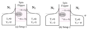
Figure 3: Schematic representation of a normal metal bilayer junction with a spin-flipper at the interface $x=0$, with spin-flipper’s spin $S$ and magnetic moment $m$. Temperature difference $\Delta T=T_{1}-T_{2}$ is less than the average temperature $\bar{T}=(T_{1}+T_{2})/2$, i.e., $T_{1}$ is comparable to $T_{2}$ with (a) setup 1, at zero bias voltage $V_{1}=V_{2}=V$, (b) setup 2, at finite bias voltage $V_{1}=0$, $V_{2}=-\mu$.

In Fig. 3, we represent our chosen setups to study spin-polarized $\Delta_{T}$ noise in N₁/SF/N₂ junction. Here, we take temperature in normal metal $N_{1}$ as $T_{1}$, and in normal metal $N_{2}$ as $T_{2}$ with $T_{1}\neq T_{2}\neq 0$ and temperature difference $\Delta T=T_{1}-T_{2}$ is much smaller than average temperature $\bar{T}=(T_{1}+T_{2})/2$. First, we review the zero bias case, i.e., applied bias $\Delta V=V_{1}-V_{2}=0$, the voltage in $N_{1}$ is $V_{1}=V$ and $N_{2}$ is $V_{2}=V$ defined as setup 1 in Fig. 3(a). The finite voltage case $V_{1}=0$ and $V_{2}=-\mu$ is defined as setup 2, shown in Fig. 3(b). Thermovoltage $\mu$ is the applied bias voltage required to tune the average charge (spin) current to zero ($I^{ch(sp)}_{1}=0$) [12]. To calculate $\Delta^{\eta}_{T}$ ($\eta=ch,sp,N$) noise, we simplify the $\Delta^{\eta}_{T}$ noise in power series of gradient expansion factor $\left(\frac{\Delta T}{2\bar{T}}\right)$. In this paper, for comparable reservoir setups, we have taken temperature configurations, implying $\frac{\Delta T}{2\bar{T}}\approx 0.14$. For setup 1, i.e., zero bias case ($\Delta V=V_{1}-V_{2}=0$), Fermi distribution function in $N_{1}$ is $f_{1}(E-V)=\left[1+e^{\frac{E-V}{k_{B}T_{1}}}\right]^{-1}$ and in $N_{2}$ is $f_{2}(E-V)=\left[1+e^{\frac{E-V}{k_{B}T_{2}}}\right]^{-1}$. Hence both Fermi functions $f_{1}(E-V)$ and $f_{2}(E-V)$ differ by their temperatures ($T_{1}\neq T_{2}$). For setup 2, i.e., finite bias case ($V_{1}=0$,$V_{2}\neq 0$), Fermi functions can be written as $f_{1}(E)=\left[1+e^{\frac{E}{k_{B}T_{1}}}\right]^{-1}$ and $f_{2}(E-V_{2})=\left[1+e^{\frac{E-V_{2}}{k_{B}T_{2}}}\right]^{-1}$.

The total charge $\Delta_{T}$ and spin $\Delta_{T}$ noises are, $\Delta^{ch}_{T}(T_{1},T_{2})=\Delta^{ch}_{Tth}(T_{1},T_{2})+\Delta^{ch}_{Tsh}(T_{1},T_{2})$ and $\Delta^{sp}_{T}(T_{1},T_{2})=\Delta^{sp}_{Tth}(T_{1},T_{2})+\Delta^{sp}_{Tsh}(T_{1},T_{2})$ respectively. Without any spin-flip scattering for NIN junction, both charge and spin $\Delta_{T}$ noises are identical, i.e., $\Delta^{N}_{T}(T_{1},T_{2})=\Delta^{ch}_{T}(T_{1},T_{2})=\Delta^{sp}_{T}(T_{1},T_{2})=\Delta^{N}_{Tth}(T_{1},T_{2})+\Delta^{N}_{Tsh}(T_{1},T_{2})$. To derive $\Delta_{T}$ noise analytically, we make the assumption that the temperatures of the reservoirs are much smaller than the energy scale of the transmission probability, i.e., $\frac{k_{B}\bar{T}}{cJ^{2}_{0}}\ll 1$.

II.4.1 Setup 1:

First, we study both the setups of Fig. 3. Shot noise-like contribution to the $\Delta^{\eta}_{T}$ noise ($\Delta^{\eta}_{Tsh}$) is calculated from $S^{\eta}_{11sh}$, as discussed in section II.2 and Eq. (33). By utilizing the condition of vanishing current and replacing the thermovoltage (Eqs. 50, 51, and 52), for temperature configurations $\frac{\Delta T}{2\bar{T}}\ll 1$ and zero bias in setup 1, with the approximation $\frac{k_{B}\bar{T}}{cJ^{2}_{0}}\ll 1$, $\Delta^{\eta}_{Tsh}$ is derived as,

$$\Delta^{\eta}_{Tsh} =\frac{2e^{2}}{h}k_{B}\bar{T}\biggl{[}4\biggl{\{}F^{\eta}_{11sh}\left(\frac{V}{cJ^{2}_{0}}\right)\frac{\pi^{2}-6}{9}-\left(\frac{k_{B}\bar{T}}{cJ^{2}_{0}}\right)^{2}\left(F^{\eta}_{11sh}\left(\frac{V}{cJ^{2}_{0}}\right)\right)^{(2)}$$ (34)

$$\frac{\pi^{2}(7\pi^{2}-60)}{45}\biggr{\}}\left(\frac{\Delta T}{2\bar{T}}\right)^{2}+\frac{4}{3}\biggl{\{}F^{\eta}_{11sh}\left(\frac{V}{cJ^{2}_{0}}\right)\frac{75\pi^{2}-7\pi^{4}-90}{675}$$

$$-\left(\frac{k_{B}\bar{T}}{cJ^{2}_{0}}\right)^{2}\left(F^{\eta}_{11sh}\left(\frac{V}{cJ^{2}_{0}}\right)\right)^{(2)}\leavevmode\nobreak\ \frac{294-31\pi^{2}}{630}\biggr{\}}\left(\frac{\Delta T}{2\bar{T}}\right)^{4}\biggr{]}+O\left(\frac{\Delta T}{2\bar{T}}\right)^{6},\leavevmode\nobreak\ \leavevmode\nobreak\ \leavevmode\nobreak\ \leavevmode\nobreak\$$

where $\eta=ch,sp$ denotes the charge and spin in N₁/SF/N₂ junction, and $\eta=N$ denotes the NIN junction without any spin-flip scattering (see Appendix C, Eqs. (82), (86), and (88) for detailed derivation. $F^{\eta}_{11sh}$ is function of reflection and transmission amplitudes, with $F^{ch}_{11sh}=F^{\uparrow\uparrow}_{11sh}+F^{\uparrow\downarrow}_{11sh}+F^{\downarrow\uparrow}_{11sh}+F^{\downarrow\downarrow}_{11sh}$. Similarly, $F^{sp}_{11sh}=F^{\uparrow\uparrow}_{11sh}-F^{\uparrow\downarrow}_{11sh}-F^{\downarrow\uparrow}_{11sh}$ + $F^{\downarrow\downarrow}_{11sh}$ is the spin shot noise contribution. Expressions for $F^{\sigma\sigma^{\prime}}_{11sh}$ are given below,

$$F^{\uparrow\uparrow}_{11sh} = |s^{\uparrow\uparrow}_{12}|^{2}|s^{\uparrow\uparrow}_{11}|^{2}+2Re[s^{\uparrow\uparrow\dagger}_{11}s^{\uparrow\downarrow}_{12}s^{\uparrow\uparrow\dagger}_{12}s^{\uparrow\downarrow}_{11}]+|s^{\uparrow\downarrow}_{12}|^{2}|s^{\uparrow\downarrow}_{11}|^{2},\leavevmode\nobreak\ \leavevmode\nobreak\ \leavevmode\nobreak\ \leavevmode\nobreak\ F^{\downarrow\downarrow}_{11sh}=|s^{\downarrow\downarrow}_{12}|^{2}|s^{\downarrow\downarrow}_{11}|^{2}+2Re[s^{\downarrow\downarrow\dagger}_{11}s^{\downarrow\uparrow}_{12}s^{\downarrow\downarrow\dagger}_{12}s^{\downarrow\uparrow}_{11}]+|s^{\downarrow\uparrow}_{12}|^{2}|s^{\downarrow\uparrow}_{12}|^{2},$$

$$F^{\uparrow\downarrow}_{11sh} = 2Re[s^{\uparrow\downarrow\dagger}_{11}s^{\uparrow\uparrow}_{12}s^{\downarrow\downarrow\dagger}_{12}s^{\downarrow\uparrow}_{11}]+2Re[s^{\uparrow\uparrow\dagger}_{11}s^{\uparrow\downarrow}_{12}s^{\downarrow\downarrow\dagger}_{12}s^{\downarrow\uparrow}_{11}]+2Re[s^{\uparrow\uparrow\dagger}_{12}s^{\uparrow\downarrow}_{11}s^{\downarrow\downarrow\dagger}_{11}s^{\downarrow\uparrow}_{12}]+2Re[s^{\uparrow\downarrow\dagger}_{11}s^{\uparrow\downarrow}_{12}s^{\downarrow\uparrow\dagger}_{12}s^{\downarrow\uparrow}_{11}],$$

$$F^{\downarrow\uparrow}_{11sh} = 2Re[s^{\downarrow\uparrow\dagger}_{11}s^{\downarrow\downarrow}_{12}s^{\uparrow\uparrow\dagger}_{12}s^{\uparrow\downarrow}_{11}]+2Re[s^{\downarrow\downarrow\dagger}_{11}s^{\downarrow\uparrow}_{12}s^{\uparrow\uparrow\dagger}_{12}s^{\uparrow\downarrow}_{11}]+2Re[s^{\downarrow\downarrow\dagger}_{12}s^{\downarrow\uparrow}_{11}s^{\uparrow\uparrow\dagger}_{11}s^{\uparrow\downarrow}_{12}]+2Re[s^{\downarrow\uparrow\dagger}_{11}s^{\downarrow\uparrow}_{12}s^{\uparrow\downarrow\dagger}_{12}s^{\uparrow\downarrow}_{11}],$$ (35)

$$\text{wherein Re[...] is Real part of the product of scattering amplitudes},$$

and given in Appendix B, Eq. (77). Thermal noise-like contribution to the $\Delta^{\eta}_{T}$ noise, i.e., $\Delta^{\eta}_{Tth}$ is derived from $S^{\eta}_{11th}$, as mentioned in section II.2 and Eq.33. For vanishing current condition, replacing the thermovoltage (Eqs. 50, 51, and 52), for $\frac{\Delta T}{2\bar{T}}\ll 1$ and zero bias in setup 1, with approximation $\frac{k_{B}\bar{T}}{cJ^{2}_{0}}\ll 1$, $\Delta^{\eta}_{Tth}$ can be written as,

$$\Delta^{\eta}_{Tth} = \frac{2e^{2}}{h}k_{B}\bar{T}\biggl{[}2F^{\eta}_{11th}\left(\frac{V}{cJ^{2}_{0}}\right)+2\sum^{\infty}_{n=1}\left(\frac{k_{B}\bar{T}}{cJ^{2}_{0}}\right)^{2n}\left(F^{\eta}_{11th}\left(\frac{V}{cJ^{2}_{0}}\right)\right)^{(2n)}(2-4^{1-n})\zeta(2n)+\biggl{\{}\left(\frac{k_{B}\bar{T}}{cJ^{2}_{0}}\right)^{2}\left(F^{\eta}_{11th}\left(\frac{V}{cJ^{2}_{0}}\right)\right)^{(2)}\frac{\pi^{2}}{3}\biggr{\}}\left(\frac{\Delta T}{2\bar{T}}\right)^{2}$$ (36)

$$+\left(\frac{k_{B}\bar{T}}{cJ^{2}_{0}}\right)^{2}\biggl{\{}\left(F^{\eta}_{11th}\left(\frac{V}{cJ^{2}_{0}}\right)\right)^{(2)}\frac{\pi^{2}}{135}\left(120+7\pi^{2}\right)-\frac{7\pi^{4}}{5}\left(F^{\eta}_{11th}\left(\frac{V}{cJ^{2}_{0}}\right)\right)^{(2)}\biggr{\}}\left(\frac{\Delta T}{2\bar{T}}\right)^{4}\biggr{]}+O\left(\frac{\Delta T}{2\bar{T}}\right)^{6},$$

where $\zeta$ is Riemann zeta function, see Appendix C, Eqs.(84), (85) and (87) for derivation of $\Delta^{\eta}_{Tth}$. Derivation of the thermovoltage $\mu$ for setup 1 is given in Appendix A, Eq. (50). $(F^{\eta}_{11th})^{(2n)}$ is the $(2n)$th derivative of $F^{\eta}_{11th}$ with respect to energy. $F^{\eta}_{11th}$ is dependent on reflection and transmission amplitudes, with $F^{ch}_{11th}=F^{\uparrow\uparrow}_{11th}+F^{\uparrow\downarrow}_{11th}+F^{\downarrow\uparrow}_{11th}$ + $F^{\downarrow\downarrow}_{11th}$. Similarly, $F^{sp}_{11th}=F^{\uparrow\uparrow}_{11th}-F^{\uparrow\downarrow}_{11th}-F^{\downarrow\uparrow}_{11th}$ + $F^{\downarrow\downarrow}_{11th}$. Expressions for $F^{\sigma\sigma^{\prime}}_{11th}$ are given as,

$$F^{\uparrow\uparrow}_{11th} = |s^{\uparrow\uparrow}_{12}|^{2}|s^{\downarrow\downarrow}_{12}|^{2}+2Re[s^{\uparrow\uparrow\dagger}_{11}s^{\uparrow\downarrow}_{12}s^{\uparrow\uparrow\dagger}_{11}s^{\uparrow\downarrow}_{11}]+|s^{\uparrow\downarrow}_{11}|^{2}|s^{\downarrow\uparrow}_{11}|^{2},\leavevmode\nobreak\ \leavevmode\nobreak\ \leavevmode\nobreak\ \leavevmode\nobreak\ F^{\uparrow\downarrow}_{11th}=(1-|s^{\uparrow\downarrow}_{11}|^{2})(1-|s^{\downarrow\uparrow}_{11}|^{2})+2Re[s^{\uparrow\uparrow\dagger}_{11}s^{\uparrow\downarrow}_{11}s^{\downarrow\downarrow\dagger}_{11}s^{\downarrow\uparrow}_{11}]+|s^{\downarrow\uparrow\dagger}_{11}|^{2}|s^{\uparrow\downarrow}_{11}|^{2},$$

$$F^{\downarrow\uparrow}_{11th} = (1-|s^{\downarrow\uparrow}_{11}|^{2})(1-|s^{\uparrow\downarrow}_{11}|^{2})+2Re[s^{\downarrow\downarrow\dagger}_{11}s^{\downarrow\uparrow}_{11}s^{\uparrow\uparrow\dagger}_{11}s^{\uparrow\downarrow}_{11}]+|s^{\uparrow\downarrow\dagger}_{11}|^{2}|s^{\downarrow\uparrow}_{11}|^{2},\leavevmode\nobreak\ \leavevmode\nobreak\ \leavevmode\nobreak\ F^{\downarrow\downarrow}_{11th}=|s^{\downarrow\downarrow}_{12}|^{2}|s^{\uparrow\uparrow}_{12}|^{2}+2Re[s^{\downarrow\downarrow\dagger}_{11}s^{\downarrow\uparrow}_{12}s^{\downarrow\downarrow\dagger}_{11}s^{\downarrow\uparrow}_{11}]+|s^{\downarrow\uparrow}_{11}|^{2}|s^{\uparrow\downarrow}_{11}|^{2},$$ (37)

given in Appendix B, Eq. (78). Now energy $E$ for charge carriers can be defined as $E=k_{B}\bar{T}\omega$, which is useful for simplifying integrations that involve Fermi functions and explained in Eq. (48) for the calculation of current in setup 1. The same technique is also used for determining the current and $\Delta_{T}$ noise, as explained in detail in Appendix A and C, respectively for all setups. We calculate $\Delta^{\eta}_{Tsh(Tth)}$ noise analytically using a Taylor series expansion of $F^{\eta}_{11sh(11th)}$ in powers of $\frac{k_{B}\bar{T}}{cJ^{2}_{0}}$, i.e., $F^{\eta}_{11sh(11th)}\left(\frac{k_{B}\bar{T}\omega}{cJ^{2}_{0}}\right)=\sum^{n=\infty}_{n=0}(F^{\eta}_{11sh(11th)}(0))^{(n)}\frac{(k_{B}\bar{T}\omega)^{n}}{n!(cJ^{2}_{0})^{n}}$, where $\eta$ denotes $ch,\leavevmode\nobreak\ sp$ or $N$. When the approximation $\frac{k_{B}\bar{T}}{cJ^{2}_{0}}\ll 1$ is valid, we can disregard higher-order terms of $\frac{k_{B}\bar{T}}{cJ^{2}_{0}}$ without affecting the results, see Appendix C for detailed derivation see Eqs. (82-99). Coefficients of odd powers of $\left(\frac{\Delta T}{2\bar{T}}\right)$ in $\Delta^{\eta}_{Tsh}$ vanishes at zero bias in setup 1 as $V_{1}=V_{2}=V$.

II.4.2 Setup 2:

Similar to setup 1, we can obtain $\Delta^{\eta}_{T}$ noise for setup 2 under the temperature configuration $\mid\frac{\Delta T}{2\bar{T}}\mid\ll 1$, at finite bias and with the approximation $\mid\frac{k_{B}\bar{T}}{cJ^{2}_{0}}\mid\ll 1$. Shot noise-like contribution to the $\Delta^{\eta}_{T}$ noise ($\Delta^{\eta}_{Tsh}$) is calculated from $S^{\eta}_{11sh}$, as discussed in section II.2 and Eq.33, by substituting the thermovoltage for zero current (Eqs. 57, 58, and 59), and can be simplified as,

$$\Delta^{\eta}_{Tsh} = \frac{2e^{2}}{h}k_{B}\bar{T}\biggl{[}\biggl{\{}-\left(F^{\eta}_{11sh}(0)+F^{\eta}_{11sh}\left(\frac{V_{2}}{cJ^{2}_{0}}\right)\right)+\frac{k_{B}\bar{T}}{cJ^{2}_{0}}\left((F^{\eta}_{11sh}(0))^{(1)}+\left(F^{\eta}_{11sh}\left(\frac{V_{2}}{cJ^{2}_{0}}\right)\right)^{(1)}\right)\frac{\pi^{2}}{3}-\left(\frac{k_{B}\bar{T}}{cJ^{2}_{0}}\right)^{2}\frac{\pi^{2}}{6}\left((F^{\eta}_{11sh}(0))^{(2)}\right.$$ (38)

$$\left.+\left(F^{\eta}_{11sh}\left(\frac{V_{2}}{cJ^{2}_{0}}\right)\right)^{(2)}\right)\biggr{\}}\left(\frac{\Delta T}{2\bar{T}}\right)+\biggl{\{}\frac{k_{B}\bar{T}}{cJ^{2}_{0}}\left((F^{\eta}_{11sh}(0))^{(1)}+\left(F^{\eta}_{11sh}\left(\frac{V_{2}}{cJ^{2}_{0}}\right)\right)^{(1)}\right)\frac{\pi^{2}}{3}-\left(\frac{k_{B}\bar{T}}{cJ^{2}_{0}}\right)^{2}\frac{\pi^{2}(7\pi^{2}-15)}{90}\left((F^{\eta}_{11sh}(0))^{(2)}\right.$$

$$\left.+\left(F^{\eta}_{11sh}\left(\frac{V_{2}}{cJ^{2}_{0}}\right)\right)^{(2)}\right)\biggr{\}}\left(\frac{\Delta T}{2\bar{T}}\right)^{2}\biggr{]}+O\left(\frac{\Delta T}{2\bar{T}}\right)^{3},$$

where $\left(F^{\eta}_{11sh}\left(\frac{V_{2}}{cJ^{2}_{0}}\right)\right)^{(n)}$ denotes the $n$th derivative of $F^{\eta}_{11sh}\left(\frac{V_{2}}{cJ^{2}_{0}}\right)$ with respect to dimesnionless energy $\frac{E}{cJ^{2}_{0}}$ at applied voltage $\frac{V_{2}}{cJ^{2}_{0}}$. $V_{2}$ in $\Delta^{\eta}_{Tsh}$ is replaced by thermovoltage $-\mu$ to tune the current to zero. The detailed derivation of $\Delta^{\eta}_{Tsh}$ for setup 2 is given in Appendix C, see Eqs. (92), (98), and (100). Thermal noise-like contribution to $\Delta^{\eta}_{T}$, i.e., $\Delta^{\eta}_{Tth}$ is derived from $S^{\eta}_{11sh}$, as discussed in section II.2 and Eq.33 for $\mid\frac{\Delta T}{2\bar{T}}\mid\ll 1$, at finite bias is written as,

$$\Delta^{\eta}_{Tth} = \frac{2e^{2}}{h}k_{B}\bar{T}\biggl{[}\biggl{\{}2F^{\eta}_{11th}(0)\left(1+\frac{\Delta T}{2\bar{T}}\right)+2F^{\eta}_{11th}\left(\frac{V_{2}}{cJ^{2}_{0}}\right)\left(1-\frac{\Delta T}{2\bar{T}}\right)+4\left(\frac{k_{B}\bar{T}}{cJ^{2}_{0}}\right)^{2}\left((F^{\eta}_{11th}(0))^{(2)}\left(1+\frac{\Delta T}{2\bar{T}}\right)+\left(F^{\eta}_{11th}\left(\frac{V_{2}}{cJ^{2}_{0}}\right)\right)^{(2)}\right)\zeta(2)$$ (39)

$$\left(1-\frac{\Delta T}{2\bar{T}}\right)\biggr{\}}+\frac{\pi^{2}}{3}\left(\frac{k_{B}\bar{T}}{cJ^{2}_{0}}\right)^{2}\biggl{\{}\left((F^{\eta}_{11th}(0))^{(2)}\left(1+\frac{\Delta T}{2\bar{T}}\right)-\left(F^{\eta}_{11th}\left(\frac{V_{2}}{cJ^{2}_{0}}\right)\right)^{(2)}\left(1-\frac{\Delta T}{2\bar{T}}\right)\right)\biggr{\}}\left(\frac{\Delta T}{2\bar{T}}\right)+\frac{\pi^{2}}{6}\biggl{\{}\left(\frac{k_{B}\bar{T}}{cJ^{2}_{0}}\right)^{2}\left((F^{\eta}_{11th}(0))^{(2)}\right.$$

$$\left.\left(1+\frac{\Delta T}{2\bar{T}}\right)+\left(F^{\eta}_{11th}\left(\frac{V_{2}}{cJ^{2}_{0}}\right)\right)^{(2)}\left(1-\frac{\Delta T}{2\bar{T}}\right)\right)\biggr{\}}\left(\frac{\Delta T}{2\bar{T}}\right)^{2}+O\left(\frac{\Delta T}{2\bar{T}}\right)^{3}.$$

$V_{2}$ in $\Delta^{\eta}_{Tth}$ is replaced by thermovoltage $-\mu$ to tune the current to zero. The detailed derivation of $\Delta^{\eta}_{Tth}$ for setup 2 is given in Appendix C, see Eqs. (96), (97), and (99). Thermovoltage $V_{2}=-\mu$ is derived in Appendix A, see Eqs. (57, 58, and 59), by imposing the vanishing charge current condition. Next, we discuss the case of one hot and the other cold reservoir.

II.5 Spin-polarized $\Delta_{T}$ noise: one hot and the other cold reservoir (setups 3 & 4)

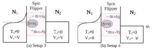
Figure 4: Schematic presentation of a normal metal bilayer junction with a spin-flipper at the interface $x=0$, spin-flipper’s spin $S$, and spin magnetic moment $m$. Temperatures of two reservoirs are: $T_{1}>0$, $T_{2}=0$, (a) setup 3, with zero bias voltage $V_{1}=V_{2}=V$, (b) setup 4, with finite bias voltage $V_{1}=0$, $V_{2}=-\mu$.

In Fig. 4, we represent the other two setups, for one hot reservoir (at finite temperature) and the other cold reservoir (at zero temperature) to study spin-polarized $\Delta_{T}$ noise in N₁/SF/N₂ junction.

In $\Delta_{T}$ noise calculation for one hot and the other cold reservoir, the temperature gradient factor $\frac{\Delta T}{2\bar{T}}\equiv 1$ as $\Delta T=T_{1}=T$ and $\bar{T}=T_{1}/2=T/2$, Hence, the $\Delta_{T}$ noise expansion with temperature gradient power series $\left(\frac{\Delta T}{2\bar{T}}\right)$ is not valid anymore and is reduced to an expansion as a series of $T$. Here in this paper, for one hot and the other cold reservoir case, we have taken $T_{1}=T$, $T_{2}=0$. The zero bias case $\Delta V=0$, i.e., applied bias in both $N_{1}$ is $V_{1}=V$ and in $N_{2}$ is $V_{2}=V$, is setup 3 in Fig. 4(a), and the setup 4 is for finite voltage case $V_{1}=0$ and thermovoltage $V_{2}=-\mu$ in Fig. 4(b). For setup 3, Fermi functions in $N_{1}$ is $f_{1}(E-V)=\left[1+e^{\frac{E-V}{k_{B}T}}\right]^{-1}$ and in $N_{2}$ is $f_{2}(E-V)=\Theta(-E+V)$, and for setup 4, $f_{1}(E)=\left[1+e^{\frac{E}{k_{B}T}}\right]^{-1}$ and $f_{2}(E-V_{2})=\Theta(-E+V_{2})$, where $\Theta$ is Heaviside step function. Similar to the cases of reservoirs with comparable temperatures, to calculate $\Delta_{T}$ noise analytically for the one hot and other cold reservoir, we assume that the temperatures of the reservoirs are much smaller than the energy scale of the transmission probability, i.e., $\mid\frac{k_{B}T}{cJ^{2}_{0}}\mid\ll 1$.

II.5.1 Setup 3:

For zero bias, i.e., setup 3 in Fig. 4(a), $\Delta^{\eta}_{Tth}$ contribution to the $\Delta^{\eta}_{T}$ noise can be derived from $S^{\eta}_{11th}$ (see Eq. 33 and section II.2) by substituting the thermovoltage for vanishing current with temperature and voltage configurations specified in setup 3 with the approximation $\mid\frac{k_{B}T}{cJ^{2}_{0}}\mid\ll 1$, and can be written as,

$$\Delta^{\eta}_{Tth} = \frac{2e^{2}}{h}k_{B}T\left(F^{\eta}_{11th}\left(\frac{V}{cJ^{2}_{0}}\right)+2\left(\frac{k_{B}T}{cJ^{2}_{0}}\right)^{2}\left(F^{\eta}_{11th}\left(\frac{V}{cJ^{2}_{0}}\right)\right)^{(2)}\zeta(2)\right),$$ (40)

the detailed derivation of $\Delta^{\eta}_{Tth}$ for setup 3 is given in Appendix C, Eqs.(105), (107), and (109). Shot noise-like contribution $\Delta^{\eta}_{Tsh}$ to the $\Delta^{\eta}_{T}$ noise is calculated from $S^{\eta}_{11sh}$ (see Eq. 33 and section II.2) by substituting the thermovoltage for vanishing current in setup 3 with the approximation $\mid\frac{k_{B}T}{cJ^{2}_{0}}\mid\ll 1$ is derived as,

$$\Delta^{\eta}_{Tsh}=\frac{2e^{2}}{h}k_{B}T\biggl{[}F^{\eta}_{11sh}\left(\frac{V}{cJ^{2}_{0}}\right)\left(2\ln 2-1+d_{0}\right)+2\left(\frac{k_{B}T}{cJ^{2}_{0}}\right)^{2}\left(F^{\eta}_{11sh}\left(\frac{V}{cJ^{2}_{0}}\right)\right)^{(2)}\left(\frac{3\zeta(3)}{8}-\zeta(2)+d_{2}\right)-\left(\frac{k_{B}T}{cJ^{2}_{0}}\right)\left(F^{\eta}_{11sh}\left(\frac{V}{cJ^{2}_{0}}\right)\right)^{(1)}d_{1}\biggr{]},\leavevmode\nobreak\ \leavevmode\nobreak\ \leavevmode\nobreak\ \leavevmode\nobreak\ \leavevmode\nobreak\$$ (41)

where $d_{0}=\left(\frac{V}{k_{B}T}\right)^{2}-\frac{1}{24}\left(\frac{V}{k_{B}T}\right)^{4}$, $d_{1}=2\left(\frac{V}{2k_{B}T}\right)^{3}$, and $d_{2}=\left(\frac{V}{2k_{B}T}\right)^{4}$ and for its detailed derivation see Appendix C, Eqs.(104), (106), and (108). Here $\eta=ch,sp$ is for charge and spin in N₁/SF/N₂ junction and $\eta=N$ is for NIN junction without any spin-flip scattering, $(F^{\eta}_{11th})^{(n)}$ denotes the $n$th derivative of $F^{\eta}_{11th}$ with respect to energy $\frac{E}{cJ^{2}_{0}}$. For spin $\Delta^{ch(sp)}_{Tth}$, we consider charge (spin) scattering term $F^{ch(sp)}_{11th}$ in Eq. (40), see Appendix B, Eqs. (77) and  (78) for detailed derivation of $F^{ch}_{11th}$ and $F^{sp}_{11th}$. In NIN junction, the charge and spin noise are the same without spin-flip scattering. The thermovoltage for finite bias setup 3 is given in Eqs. (64,65, and 66).

II.5.2 Setup 4:

For finite bias setup, i.e., setup 4 of Fig. 4(b), $\Delta^{\eta}_{Tth}$ noise is calculated from $S^{\eta}_{11th}$ (see Eq. 33 and section II.2) by substituting the thermovoltage (Eqs. 71, 72, and 73) for vanishing current in setup 4, with the approximation $\mid\frac{k_{B}T}{cJ^{2}_{0}}\mid\ll 1$ is given as,

$$\Delta^{\eta}_{Tth} =\frac{2e^{2}}{h}k_{B}T\left(F^{\eta}_{11th}(0)+2\left(\frac{k_{B}T}{cJ^{2}_{0}}\right)^{2}(F^{\eta}_{11th}(0))^{(2)}\zeta(2)\right),\leavevmode\nobreak\ \leavevmode\nobreak\ \leavevmode\nobreak\$$ (42)

which is derived in Appendix C, see Eqs.(114), (116), and (118). $\Delta^{\eta}_{Tsh}$ is calculated from $S^{\eta}_{11sh}$ as mentioned in Eq. 33 and section II.2, by substituting the thermovoltage for vanishing current in finite bias setup 4, with the approximation $\mid\frac{k_{B}T}{cJ^{2}_{0}}\mid\ll 1$ is given as,

$$\Delta^{\eta}_{Tsh} = \frac{2e^{2}}{h}k_{B}T\biggl{[}F^{\eta}_{11sh}(0)\left(2\ln(2)-1+d_{0}\right)+\frac{k_{B}T}{cJ^{2}_{0}}(F^{\eta}_{11sh}(0))^{(1)}d_{1}$$ (43)

$$+2\left(\frac{k_{B}T}{cJ^{2}_{0}}\right)^{2}(F^{\eta}_{11sh}(0))^{(2)}\left(\frac{3\zeta(3)}{8}-\zeta(2)+d_{2}\right)\biggr{]},$$

where $d_{0}$, $d_{1}$ and $d_{2}$ are functions of $\frac{V_{2}}{k_{B}T}$ instead of $\frac{V}{k_{B}T}$. At voltage $V_{2}$ is replaced by thermovoltage $-\mu$ in $\Delta^{\eta}_{Tsh}$, see Appendix C, Eqs.(96), (97), and (99) for detailed derivation. Expressions for thermovoltage $\mu$ for vanishing current condition for respective $\Delta^{\eta}_{T}$ noise, with $\eta=ch,sp,N$ in setup 4 is given in Appendix A, see Eqs. (71, 72, 73). $\Delta^{\eta}_{Tth}$ remains independent of voltages for finite bias in setup 4.

General bounds for the charge as well as spin noise with spin-flip scattering and NIN case in the absence of spin-flip scattering, i.e., the ratio of charge (spin or NIN) shot noise-like contribution to charge (spin or NIN) thermal noise-like contribution at zero charge (spin or NIN) current condition has been verified, i.e., $\mid\frac{\Delta^{ch}_{Tsh}}{\Delta^{ch}_{Tth}}\mid<1$, $\mid\frac{\Delta^{sp}_{Tsh}}{\Delta^{sp}_{Tth}}\mid<1$ and $\mid\frac{\Delta^{N}_{Tsh}}{\Delta^{N}_{Tth}}\mid<1$ [12]. In the next section, we plot results of $\Delta^{\eta}_{T}$ noise with the ratio $\mid\frac{\Delta^{\eta}_{Tsh}}{\Delta^{\eta}_{Tth}}\mid$ for each setup.

III Results and Discussion

This section discusses the results of charge $\Delta_{T}$ noise and spin $\Delta_{T}$ noise for each setup. We discuss $\Delta^{\eta}_{T}$ noise ($\eta=ch,sp,N$) along with the ratio of shot noise-like contribution to thermal noise-like contribution for reservoir with comparable temperatures cases (setups 1 and 2) in subsection A, followed by one hot and the other cold reservoir cases (setups 3 and 4) in subsection B. The spin-flipper’s spin $S=1/2$ for all plots and setups considered.

Table 1: Temperature and voltage parameters for each setup.

Temperature	Setup	Voltage	$\Delta^{\eta}_{T}$	$|\Delta^{\eta}_{Tsh}/\Delta^{\eta}_{Tth}|$
Reservoirs at comparable temperatures ($\Delta T\ll 2\bar{T}$,  $\frac{\Delta T}{2\bar{T}}\approx 0.14$)	1	$\Delta V=0$	Fig. 5 (a)	Fig. 5 (b)
	2	$V_{1}=0$ $V_{2}=-\mu$	Fig. 6 (a)	Fig. 6 (b)
Hot and cold reservoir ($T_{1}>T_{2}$,  $\frac{\Delta T}{2\bar{T}}=1$)	3	$\Delta V=0$	Fig. 7 (a)	Fig. 7 (b)
	4	$V_{1}=0$ $V_{2}=-\mu$	Fig. 8 (a)	Fig. 8 (b)

We evaluate the thermovoltage for each spin-configuration shown in Fig. 2 and calculate the respective $\Delta_{T}$ noise (see Appendix A and C for detailed calculation). We plot $\Delta^{\eta}_{T}$ noise, $\eta=ch,sp,N$ versus the dimensionless parameter $\frac{k_{B}\bar{T}}{cJ^{2}_{0}}$, for a fixed value of the spin-flipper’s spin $S$ and take the sum over all possible spin magetic moment $m=-S,-S+1/2,...,S-1/2,S$ values. Charge $\Delta^{ch}_{T}$ noise and the ratio $\mid\frac{\Delta^{ch}_{Tsh}}{\Delta^{ch}_{Tth}}\mid$ are denoted by black lines, similarly spin $\Delta^{sp}_{T}$ noise and the ratio $\mid\frac{\Delta^{sp}_{Tsh}}{\Delta^{sp}_{Tth}}\mid$ are denoted by blue lines and for NIN junction $\Delta^{N}_{T}$ noise and the ratio $\mid\frac{\Delta^{N}_{Tsh}}{\Delta^{N}_{Tth}}\mid$ are denoted by red lines in Figs. (5,6,7,8).

III.1 $\Delta^{\eta}_{T}$ noise in reservoirs with comparable temperatures

In Fig. 5 for setup 1, we plot $\Delta^{\eta}_{T}$ and the ratio $|\Delta^{\eta}_{Tsh}/\Delta^{\eta}_{Tth}|$ vs. dimensionless parameter $\frac{k_{B}\bar{T}}{cJ^{2}_{0}}$ for $\frac{\Delta T}{2\bar{T}}\simeq 0.14$, where $\eta=ch,sp$ and $N$. In the absence of spin-flip scattering, the $\Delta^{N}_{T}$ noise remains positive regardless of changes in $\frac{k_{B}\bar{T}}{cJ^{2}_{0}}$, see the inset in Fig. 5(a). Similarly, spin noise $\Delta^{sp}_{T}$ is positive throughout in the limit $\mid\frac{k_{B}\bar{T}}{cJ^{2}_{0}}\mid\ll 1$. Conversely, the $\Delta^{ch}_{T}$ noise remains negative throughout. In the case of a NIN junction, $\Delta^{N}_{T}=\Delta^{ch}_{T}=\Delta^{sp}_{T}$ noise is consistently positive. The magnitude of the $\Delta^{N}_{Tsh}$ noise is always smaller than that of the $\Delta^{N}_{Tth}$ noise, consistent with the general bound, as described in [12]. Furthermore, even in the presence of spin-flip scattering, the charge and spin noise ratio $|\Delta^{ch(sp)}_{Tsh}/\Delta^{ch(sp)}_{Tth}|<1$, adheres to the general bound. $|\Delta^{ch(sp)}_{Tsh}/\Delta^{ch(sp)}_{Tth}|$ is very small around $\mid\frac{k_{B}\bar{T}}{cJ^{2}_{0}}\mid\rightarrow 0$, indicating that $\Delta^{ch(sp)}_{Tsh}$ vanishes. $\Delta^{ch(sp)}_{Tth}$ is larger than $\Delta^{ch(sp)}_{Tsh}$ around $\mid\frac{k_{B}\bar{T}}{cJ^{2}_{0}}\mid\rightarrow 0$ and decreases as $\frac{k_{B}\bar{T}}{cJ^{2}_{0}}$ increases. We provide a detailed explanation of this phenomenon in our analysis, with plots of shot noise and thermal noise contributions. In the case of a NIN junction, the magnitude of $\Delta^{N}_{T}$ is smaller compared to $\Delta^{ch(sp)}_{T}$, see the inset of Fig. 5(a), because both $\Delta^{N}_{Tsh}$ and $\Delta^{N}_{Tth}$ contributions are small in magnitude. However, the ratio $|\Delta^{N}_{Tsh}/\Delta^{N}_{Tth}|$ tends to zero as $\mid\frac{k_{B}\bar{T}}{cJ^{2}_{0}}\mid\rightarrow 0$ due to vanishing $\Delta^{N}_{Tsh}$, while with increasing $\mid\frac{k_{B}\bar{T}}{cJ^{2}_{0}}\mid$, it increases.

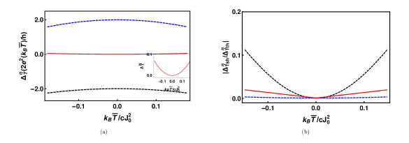
Figure 5: (a) $\Delta^{\eta}_{T}$ and (b) $|\Delta^{\eta}_{Tsh}/\Delta^{\eta}_{Tth}|$ vs. $\frac{k_{B}\bar{T}}{cJ^{2}_{0}}$ for setup 1, where $\eta=ch$ (black, dashed), $sp$ (blue, dashed) and $N$ (red, solid). The inset depicts $\Delta^{N}_{T}$ noise vs. $\frac{k_{B}\bar{T}}{cJ^{2}_{0}}$ in units of $\frac{2e^{2}(k_{B}\bar{T})}{h}$ in a narrow range.

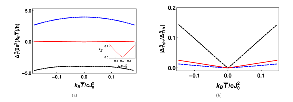
Figure 6: (a) $\Delta^{\eta}_{T}$ and (b) $|\Delta^{\eta}_{Tsh}/\Delta^{\eta}_{Tth}|$ vs. $\frac{k_{B}\bar{T}}{cJ^{2}_{0}}$ for setup 2, where $\eta=ch$ (black, dashed), $sp$ (blue, dashed) and $N$ (red, solid). The inset shows $\Delta^{N}_{T}$ noise vs. $\frac{k_{B}\bar{T}}{cJ^{2}_{0}}$ in units of $\frac{2e^{2}(k_{B}\bar{T})}{h}$ in a narrow range.

In Fig. 6, we plot $\Delta^{\eta}_{T}$ and the ratio $|\Delta^{\eta}_{Tsh}/\Delta^{\eta}_{Tth}|$ for setup 2 as function of $\frac{k_{B}\bar{T}}{cJ^{2}_{0}}$. The thermovoltage differs from setup to setup (refer to Appendix A Eqs. (50, 57)), leading to a change in the magnitude of the $\Delta^{ch}_{T}$ noise. However, since setups 1 and 2 have identical temperature gradient configurations, the $\Delta^{\eta}_{T}$ noise exhibits similar behavior. In setup 2, which includes a finite bias voltage, the $\Delta^{ch}_{T}$ noise remains negative throughout, whereas the spin noise $\Delta^{sp}_{T}$ is positive and decreases with an increase in $\frac{k_{B}\bar{T}}{cJ^{2}_{0}}$. Furthermore, both the charge and spin $\Delta^{ch(sp)}_{T}$ noise comply with the general bound, i.e., $|\Delta^{ch(sp)}_{Tsh}/\Delta^{ch(sp)}_{Tth}|<1$, as described in [12], again $|\Delta^{ch(sp)}_{Tsh}/\Delta^{ch(sp)}_{Tth}|\rightarrow 0$, as $\mid\frac{k_{B}\bar{T}}{cJ^{2}_{0}}\mid\rightarrow 0$ as . For a NIN junction, the $\Delta^{N}_{T}$ noise is always positive and exhibits behavior similar to setup 1, see the inset in Fig. 6(a). As expected, $\Delta^{N}_{T}$ noise obeys the general bound even in setup 2. Similar to setup 1, in setup 2, $|\Delta^{ch(sp)}_{Tsh}/\Delta^{ch(sp)}_{Tth}|$ vanishes at $\mid\frac{k_{B}\bar{T}}{cJ^{2}_{0}}\mid\rightarrow 0$, indicating that $\Delta^{ch(sp)}_{Tsh}$ vanishes. However, the characteristics of $|\Delta^{ch(sp)}_{Tsh}/\Delta^{ch(sp)}_{Tth}|$ differ from that of setup 1 as $\frac{k_{B}\bar{T}}{cJ^{2}_{0}}$ increases. For a NIN junction in setup 2, $|\Delta^{N}_{Tsh}/\Delta^{N}_{Tth}|$ is finite as $\frac{k_{B}\bar{T}}{cJ^{2}_{0}}$ increases similar to setup 1.

In both setups 1 and 2, the $\Delta^{ch(sp)}_{T}$ noise is symmetric as a function of $\frac{k_{B}\bar{T}}{cJ^{2}_{0}}$, as $F^{ch(sp)}_{11sh}$ and $F^{ch(sp)}_{11th}$ (given in Eq. 35 and 37), with their thermovoltages in respective setups (see Eqs. 50, 57) are functions of even powers of $\frac{k_{B}\bar{T}}{cJ^{2}_{0}}$. This property holds for the even derivatives of $F^{ch(sp)}_{11sh}$ and $F^{ch(sp)}_{11th}$, which are expressed as functions of even powers of $\frac{k_{B}\bar{T}}{cJ^{2}_{0}}$, in Eqs. (34) and (36). However, the odd derivatives of $F^{ch(sp)}_{11sh}$ and $F^{ch(sp)}_{11th}$, which arise only in setup 2, are functions of odd powers of $\frac{k_{B}\bar{T}}{cJ^{2}_{0}}$ which in turn are multiplied by an odd power expansion factor $\frac{k_{B}\bar{T}}{cJ^{2}_{0}}$, see Eqs. (38) and (39), which turns the entire expression even in $\frac{k_{B}\bar{T}}{cJ^{2}_{0}}$.

III.2 $\Delta^{\eta}_{T}$ noise with one hot and the other cold reservoir

In Fig. 7, we plot $\Delta^{\eta}_{T}$ and the ratio $|\Delta^{\eta}_{Tsh}/\Delta^{\eta}_{Tth}|$ with respect to $\frac{k_{B}T}{cJ^{2}_{0}}$, for setup 3. In contrast to setup 1 at zero bias, in setup 3, $\Delta^{ch}_{T}$ noise remains positive throughout. However, spin $\Delta^{sp}_{T}$ noise in setup 3 is consistently negative, unlike setup 1, where it is positive in the limit $\mid\frac{k_{B}T}{cJ^{2}_{0}}\mid<1$. For a NIN junction without spin-flip scattering, the behavior of $\Delta^{N}_{T}$ noise is similar to setup 1, remaining positive throughout, see the inset in Fig. 7(a). Furthermore, in setup 3, for a NIN junction, the parameters $\Delta^{N}_{Tsh}$, $\Delta^{N}_{Tth}$, and $\Delta^{N}_{T}$ remain positive regardless of any change in $\frac{k_{B}T}{cJ^{2}_{0}}$. $\Delta^{N}_{T}$ adheres to the general bound, i.e., $\mid\Delta^{N}_{Tsh}/\Delta^{N}_{Tth}\mid<1$. However, in contrast to setups 1 and 2, in setup 3 $\mid\Delta^{N}_{Tsh}/\Delta^{N}_{Tth}\mid$ exhibits a finite value as a function of $\frac{k_{B}T}{cJ^{2}_{0}}$. This is attributed to the cancellation of $\frac{k_{B}T}{cJ^{2}_{0}}$ in the ratio, resulting in a non-zero value as $\mid\frac{k_{B}T}{cJ^{2}_{0}}\mid\rightarrow 0$. Both the charge ratio $|\Delta^{ch}_{Tsh}/\Delta^{ch}_{Tth}|$ and the spin ratio $|\Delta^{sp}_{Tsh}/\Delta^{sp}_{Tth}|$ comply to the general bound described in [12]. In contrast to the cases of reservoirs with comparable temperatures, such as setup 1, in setup 3, the ratio $|\Delta^{ch(sp)}_{Tsh}/\Delta^{ch(sp)}_{Tth}|$ remains finite even at lower values of $\frac{k_{B}T}{cJ^{2}_{0}}$ due to the mutual cancellation of $\frac{k_{B}T}{cJ^{2}_{0}}$ terms. This cancellation results in an approximately constant ratio $|\Delta^{ch(sp)}_{Tsh}/\Delta^{ch(sp)}_{Tth}|$ as $\mid\frac{k_{B}T}{cJ^{2}_{0}}\mid\rightarrow 0$

The reason we plot the results in this subsection as function of $\frac{k_{B}T}{cJ^{2}_{0}}$ while in the previous subsection we plotted the results versus $\frac{k_{B}\bar{T}}{cJ^{2}_{0}}$, is because in setups 1 and 2, the scattering terms: $F^{\eta}_{I}$ (see Eqs. 44 and 45), $F^{\eta}_{Tsh}$ (see Eqs. 35) and $F^{\eta}_{Tth}$ (see Eq. 37) are expressed as functions of $\frac{k_{B}\bar{T}\omega}{cJ^{2}_{0}}$. The terms in current and $\Delta_{T}$ noise formulas involve integrals which are evaluated using Taylor series expansion of scattering terms, as functions of $\frac{k_{B}\bar{T}\omega}{cJ^{2}_{0}}$. Taking the limit $\frac{k_{B}\bar{T}}{cJ^{2}_{0}}\ll 1$, we see $\Delta^{\eta}_{T}$ noise is a function of $\frac{k_{B}\bar{T}}{cJ^{2}_{0}}$ (see Eqs. 34-39). Hence, in setups 1 and 2, we plot $\Delta^{\eta}_{T}$ noise as a function of $\frac{k_{B}\bar{T}}{cJ^{2}_{0}}$.

However, in setups 3 and 4, the scattering terms: $F^{\eta}_{I}$ (see Eqs. 44 and 45), $F^{\eta}_{Tsh}$ (see Eqs. 35) and $F^{\eta}_{Tth}$ (see Eq. 37) can be written as functions of $\frac{k_{B}T\omega}{cJ^{2}_{0}}$. To evaluate the terms involving integrals in $\Delta_{T}$ noise, we employ Taylor series expansion for the scattering terms, as function of $\frac{k_{B}T\omega}{cJ^{2}_{0}}$ with the approximation $\frac{k_{B}T}{cJ^{2}_{0}}\ll 1$, see detailed derivation in Appendix C, Eqs. (102 and 111) for $\Delta^{ch}_{Tsh}$ noise and for $\Delta^{ch}_{Tth}$ noise, see detailed derivation in Appendix C, Eqs. (105 and 114). This leads to $\Delta^{\eta}_{T}$ noise being a function of $k_{B}T/cJ^{2}_{0}$. We keep terms up to second order and disregard higher order terms of $\frac{k_{B}T}{cJ^{2}_{0}}$ (see, Eqs. 40-43). Hence, in setups 3 and 4, we plot $\Delta^{\eta}_{T}$ noise as a function of $\frac{k_{B}T}{cJ^{2}_{0}}$. We keep terms up to second order in $\frac{k_{B}\bar{T}}{cJ^{2}_{0}}$ (or $\frac{k_{B}T}{cJ^{2}_{0}}$) and neglect higher order $O\left(\frac{k_{B}\bar{T}}{cJ^{2}_{0}}\right)^{3}$ (or $O\left(\frac{k_{B}T}{cJ^{2}_{0}}\right)^{3}$) terms, as we restrict ourselves to the limit $\frac{k_{B}\bar{T}}{cJ^{2}_{0}}\ll 1$ (or $\frac{k_{B}T}{cJ^{2}_{0}}\ll 1$).

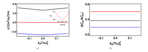
Figure 7: (a) $\Delta^{\eta}_{T}$ and (b) $|\Delta^{\eta}_{Tsh}/\Delta^{\eta}_{Tth}|$ vs. $\frac{k_{B}T}{cJ^{2}_{0}}$ for setup 3, where $\eta=ch$ (black, dashed), $sp$ (blue, dashed) and $N$ (red, solid). The inset demonstrates magnified $\Delta^{N}_{T}$ noise vs. $\frac{k_{B}\bar{T}}{cJ^{2}_{0}}$ in the unit of $\frac{2e^{2}(k_{B}T)}{h}$.

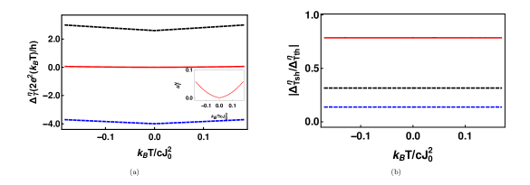
Figure 8: (a) $\Delta^{\eta}_{T}$ and (b) $|\Delta^{\eta}_{Tsh}/\Delta^{\eta}_{Tth}|$ vs. $\frac{k_{B}T}{cJ^{2}_{0}}$ for setup 4, where $\eta=ch$ (black, dashed), $sp$ (blue, dashed) and $N$ (red, solid). The inset demonstrates magnified $\Delta^{N}_{T}$ noise vs. $\frac{k_{B}\bar{T}}{cJ^{2}_{0}}$ in the unit of $\frac{2e^{2}(k_{B}T)}{h}$.

In Fig. 8, we plot $\Delta^{\eta}_{T}$ and the ratio $|\Delta^{\eta}_{Tsh}/\Delta^{\eta}_{Tth}|$ with respect to dimensionless energy parameter $\frac{k_{B}T}{cJ^{2}_{0}}$ in setup 4, i.e., finite-bias case where thermovoltage $\mu$ is imposed to ensure $I^{\eta}=0$ (as described in Appendix A4, Eqs. 50,  51, and  52). Like the other setups, $\Delta^{N}_{T}$ noise in setup 4 is positive as expected but behavior differs from setup 3, see the inset in Fig. 8(a). In contrast to finite bias setup 2, the $\Delta^{ch}_{T}$ noise in setup 4 is positive throughout. Contrary to setups 1 and 2, in setup 4, $\Delta^{sp}_{T}$ remains consistently negative in the limit $\mid\frac{k_{B}T}{cJ^{2}_{0}}\mid<1$. Both $\Delta^{ch}_{T}$ and $\Delta^{sp}_{T}$ noise in setups 3 and 4 demonstrate similar patterns due to the identical temperature gradient configuration. However, the thermovoltage varies between the two setups due to differences in the bias, leading to differences in their magnitudes. Regardless of changes in $\frac{k_{B}T}{cJ^{2}_{0}}$ or the setups considered, the $\Delta^{N}_{T}$ noise consistently exhibits positive behavior, which is expected for charge $\Delta^{ch}_{T}$ noise without spin-flip scattering, as established in previous studies [14, 15, 11]. Even in the presence of a spin-flipper, the charge (spin) $\Delta^{ch(sp)}_{T}$ noise always adheres to the general bound, with the magnitude of $\Delta^{ch(sp)}_{Tsh}$ being smaller than that of $\Delta^{ch(sp)}_{Tth}$, regardless of the setups under consideration [12]. In contrast to reservoirs with comparable temperatures, in the case of one hot and other cold reservoir (setups 3 and 4), the ratio $\mid\Delta^{ch(sp)}_{Tsh}/\Delta^{ch(sp)}_{Tth}\mid$ is finite due to the cancellation of mutual terms $\frac{k_{B}T}{cJ^{2}_{0}}$. This cancellation effect leads to a non-zero value as $\mid\frac{k_{B}T}{cJ^{2}_{0}}\mid\rightarrow 0$. Similarly, for a NIN junction in the case of one hot and other cold reservoir (setups 3 and 4), the ratio $\mid\Delta^{N}_{Tsh}/\Delta^{N}_{Tth}\mid$ also attains finite values as a function of $\frac{k_{B}T}{cJ^{2}_{0}}$.

In setups 1 and 2, $\Delta^{\eta}_{Tsh}$ (see Eqs. 34, 38 and Fig. 9) is smaller compared to $\Delta^{\eta}_{Tth}$ (see Eqs. 36, 39 and Fig. 9). Consequently, the the ratio $\mid\frac{\Delta^{\eta}_{Tsh}}{\Delta^{\eta}_{Tth}}\mid$ which is a function of $\frac{k_{B}\bar{T}}{cJ^{2}_{0}}$ is negligible when $\mid\frac{k_{B}\bar{T}}{cJ^{2}_{0}}\mid\rightarrow 0$.

However in setups 3 and 4, even though $\Delta^{\eta}_{Tsh}$ is small when $\mid\frac{k_{B}T}{cJ^{2}_{0}}\mid\rightarrow 0$ ( Fig. 10), the ratio $\mid\frac{\Delta^{\eta}_{Tsh}}{\Delta^{\eta}_{Tth}}\mid$ remains finite. Taking the ratio $\mid\frac{\Delta^{\eta}_{Tsh}}{\Delta^{\eta}_{Tth}}\mid$ common terms like $cJ^{2}_{0}$ in both denominators cancel out (see Eqs. 40-43). After replacing the thermovoltage (given in Eqs. 64-71) in bias voltage $V$ (in Eqs. 40 and 41) for setup 3 and $V_{2}$ (in Eqs. 42 and 43) for setup 4, one can simplify the expressions of $\mid\frac{\Delta^{\eta}_{Tsh}}{\Delta^{\eta}_{Tth}}\mid$ in Mathematica[20] and observe that there are terms independent of the factor $\frac{k_{B}T}{cJ^{2}_{0}}$ which give rise to finite ratio $\mid\frac{\Delta^{\eta}_{Tsh}}{\Delta^{\eta}_{Tth}}\mid$ when the limit $\mid\frac{k_{B}T}{cJ^{2}_{0}}\mid\rightarrow 0$, see Figs. 7 and  8. When $\mid\frac{k_{B}T}{cJ^{2}_{0}}\mid\rightarrow\neq 0$, we see on simplification, that it becomes evident that there are terms independent of the factor $\frac{k_{B}T}{cJ^{2}_{0}}$. These independent terms are around $20$ times larger than the ones containing the $\frac{k_{B}T}{cJ^{2}_{0}}$ factor, resulting in an almost constant value of $\mid\frac{\Delta^{\eta}_{Tsh}}{\Delta^{\eta}_{Tth}}\mid$ (see Figs. 7 and  8).

Similar to reservoirs with comparable temperatures, in case of one hot and other cold reservoir (setups 3 and 4), $\Delta^{ch}_{T}$ noise is symmetric as a function of $\frac{k_{B}T}{cJ^{2}_{0}}$. This is because $F^{ch}_{11sh}$ and $F^{ch}_{11th}$ (see Eqs. 35, and 37), in $\Delta^{ch}_{Tsh}$ and $\Delta^{ch}_{Tth}$, after replacing the thermovoltage as given in Eqs. (64, 71), are functions of even powers of $\frac{k_{B}T}{cJ^{2}_{0}}$, and also hold for the even derivatives of $F^{ch}_{11sh}$ and $F^{ch}_{11th}$, which are functions of even power of $\frac{k_{B}T}{cJ^{2}_{0}}$. However, the odd derivatives of $F^{ch}_{11sh}$ and $F^{ch}_{11th}$ are functions of odd powers of $\frac{k_{B}T}{cJ^{2}_{0}}$ and are multiplied by an odd power expansion factor $\frac{k_{B}T}{cJ^{2}_{0}}$, see in Eqs. (40-43).

Previous works on $\Delta^{N}_{T}$ noise show it to be always positive [14, 12, 11], which aligns with our results for $\Delta^{N}_{T}$. However, $\Delta^{ch}_{T}$ and $\Delta^{sp}_{T}$ turn negative due to spin-flip scattering depending on the temperature gradient of the setups. In absence of spin-flip scattering, the general bound for $\Delta^{N}_{T}$ noise is always less than $1$, i.e., $\Delta^{N}_{Tsh}<\Delta^{N}_{Tth}$, as predicted in Ref. [12]. Moreover, even in the presence of spin-flip scattering, $\Delta^{ch}_{T}$ and $\Delta^{sp}_{T}$ noise obey the general bound. The impact of temperature gradient on $\Delta_{T}$ noise is significant, as demonstrated in similar behavior of $\Delta^{ch}_{T}$ noise or $\Delta^{sp}_{T}$ noise in setups 1 and 2 with comparable temperatures, as well as in setups 3 and 4 with one hot and the other cold reservoir. On the other hand, changes in voltage configurations have minimal impact.

III.3 Leading order contributions to $\Delta_{T}$ noise

Finally, in this section we look at the leading order contributions to $\Delta_{T}$ noise and in turn the $\Delta_{Tsh}$ and $\Delta_{Tth}$ noise. $\Delta^{\eta}_{Tsh}$ noise in setup 1 (see, Eq. 34), is from $(\Delta T)^{2}$ terms, where $\eta=ch,sp$ and $N$, while for $\Delta^{\eta}_{Tth}$ noise, the leading contribution is from the average temperature, i.e., $\bar{T}$ in setup 1 (see Eq. 36). These dependencies for setup 1 are seen in a previous work [13] too, where total $\Delta^{ch}_{T}$ noise shows a clear $\bar{T}$ dependence due to dominating $\Delta^{ch}_{Tth}$ noise and excess noise, i.e., $\Delta^{ch}_{Tsh}$ noise shows $(\Delta T)^{2}$ dependence. This serves as a consistency check for our work. By measuring the total $\Delta_{T}$ noise as a function of temperature in various configurations, it is possible to observe the dominant contribution to $\Delta^{ch}_{Tth}$ noise [13]. Similarly, we find the leading order contributions in setup 2 to $\Delta^{\eta}_{Tsh}$ noise, is $\Delta T$ and to $\Delta^{\eta}_{Tth}$ noise, is $\bar{T}$ (see Eqs.  38 and 39). Furthermore, when we analyze setups 3 and 4, we see the contribution to $\Delta^{ch}_{Tsh}$ noise upto leading order is from $\Delta T$ contribution and to $\Delta^{ch}_{Tth}$ noise is from $T$ dependent (see Eqs. 40-43) terms respectively.

Table 2: Leading order contributions to $\Delta^{\eta}_{Tsh}$ and $\Delta^{\eta}_{Tth}$ noise.

Setup	$\Delta^{ch}_{Tsh}$	$\Delta^{ch}_{Tth}$	$\Delta^{sp}_{Tsh}$	$\Delta^{sp}_{Tth}$	$\Delta^{N}_{Tsh}$	$\Delta^{N}_{Tth}$
1	$\propto(\Delta T)^{2}$	$\propto\bar{T}$	$\propto(\Delta T)^{2}$	$\propto\bar{T}$	$\propto(\Delta T)^{2}$	$\propto\bar{T}$
2	$\propto(\Delta T)$	$\propto\bar{T}$	$\propto(\Delta T)$	$\propto\bar{T}$	$\propto(\Delta T)$	$\propto\bar{T}$
3	$\propto(\Delta T)$	$\propto T$	$\propto(\Delta T)$	$\propto T$	$\propto(\Delta T)$	$\propto T$
4	$\propto(\Delta T)$	$\propto T$	$\propto(\Delta T)$	$\propto T$	$\propto(\Delta T)$	$\propto T$

In Table 2, we present a summary of the maximum contributions arising from the temperature gradient ($\Delta T$) or average temperature ($\bar{T}$) terms to $\Delta^{\eta}_{Tsh}$ and $\Delta^{\eta}_{Tth}$ noise in each setup. Specifically, $\Delta T$ or $\bar{T}$ arises in derivation for setups 1 and 2, while for setups 3 and 4, it is solely $T$ since $\Delta T=T$. Terms involving $(\Delta T)^{2}$ have the greatest impact on $\Delta^{\eta}_{Tsh}$, whereas $\bar{T}$ yields the maximum contribution to $\Delta^{\eta}_{Tth}$ in setup 1, whereas in setup 2, terms involving $(\Delta T)$ have the greatest impact on $\Delta^{\eta}_{Tsh}$. Furthermore, the contributions to the $\Delta^{N}_{Tsh}$ and $\Delta^{N}_{Tth}$ noise in setup 1 exhibit a similar dependency on $(\Delta T)^{2}$ and $\bar{T}$ as observed in the case of energy-independent transmission, as discussed in Ref. [13].

IV Analysis

Table 3: Summary of the sign of $\Delta^{\eta}_{T}$, and characteristics of $\mid\frac{\Delta^{\eta}_{Tsh}}{\Delta^{\eta}_{Tth}}\mid$ as function of $\frac{k_{B}\bar{T}}{cJ^{2}_{0}}$ in each setup for $|\frac{k_{B}\bar{T}}{cJ^{2}_{0}}|<1$ with spin-flipper’s spin $S=1/2$, where $\eta=ch,\leavevmode\nobreak\ sp$ for charge and spin in N₁/SF/N₂ junction and $\eta=N$ in NIN junction.

Setup	$\Delta^{ch}_{T}$	$\mid\frac{\Delta^{ch}_{Tsh}}{\Delta^{ch}_{Tth}}\mid$ at $|\frac{k_{B}\bar{T}}{cJ^{2}_{0}}|\rightarrow 0$	$\Delta^{sp}_{T}$	$\mid\frac{\Delta^{sp}_{Tsh}}{\Delta^{sp}_{Tth}}\mid$ at $|\frac{k_{B}\bar{T}}{cJ^{2}_{0}}|\rightarrow 0$	$\Delta^{N}_{T}$	$\mid\frac{\Delta^{N}_{Tsh}}{\Delta^{N}_{Tth}}\mid$ at $|\frac{k_{B}\bar{T}}{cJ^{2}_{0}}|\rightarrow 0$
1	Negative	Vanishing	Positive	Vanishing	Positive	Vanishing
2	Negative	Vanishing	Positive	Vanishing	Positive	Vanishing
3	Positive	Finite	Negative	Finite	Positive	Finite
4	Positive	Finite	Negative	Finite	Positive	Finite

In Table 3, we have summarized the characteristics of the sign of charge $\Delta^{ch}_{T}$ noise and spin $\Delta^{sp}_{T}$ noise and the behaviour of $|\Delta^{ch(sp)}_{Tsh}/\Delta^{ch(sp)}_{Tth}|$ around $|\frac{k_{B}\bar{T}}{cJ^{2}_{0}}|\rightarrow 0$ for setups 1 and 2, and around $\mid\frac{k_{B}T}{cJ^{2}_{0}}\mid\rightarrow 0$ for setups 3 and 4. We also include the sign of $\Delta^{N}_{T}$, and behaviour of $|\Delta^{N}_{Tsh}/\Delta^{N}_{Tth}|$ at $\mid\frac{k_{B}\bar{T}}{cJ^{2}_{0}}\mid\rightarrow 0$ for setups 1 and 2, and at $\mid\frac{k_{B}T}{cJ^{2}_{0}}\mid\rightarrow 0$ for setups 3 and 4, in the absence of spin-flip scattering for a NIN junction. The limit $\mid\frac{k_{B}\bar{T}}{cJ^{2}_{0}}\mid\rightarrow 0$ or $\mid\frac{k_{B}T}{cJ^{2}_{0}}\mid\rightarrow 0$, reveals distinct characteristics of $|\Delta^{\eta}_{Tsh}/\Delta^{\eta}_{Tth}|$ for reservoirs with comparable temperatures compared to cases of one hot and other cold reservoir. The magnitude of $\mid\frac{\Delta^{\eta}_{Tsh}}{\Delta^{\eta}_{Tth}}\mid$ is almost negligible around $\frac{k_{B}\bar{T}}{cJ^{2}_{0}}\rightarrow 0$, for reservoirs with comparable temperatures. However, in the case of one hot and one cold reservoir, $\mid\frac{\Delta^{\eta}_{Tsh}}{\Delta^{\eta}_{Tth}}\mid$ is finite around $\frac{k_{B}T}{cJ^{2}_{0}}\rightarrow 0$.

$\Delta^{ch}_{T}$ noise is negative for reservoirs with comparable temperatures (setups 1 and 2), whereas positive for one hot and the other cold reservoir (setups 3 and 4). We see negative $\Delta^{ch}_{T}$ noise for the first time. Spin-flip scattering generates negative $\Delta^{ch}_{T}$ noise, due to dominant contributions from the negative $\Delta^{ch}_{Tth}$ terms, see Eqs. (36,39,40,42), although $\Delta^{ch}_{Tsh}$ contribution is completely positive, see Figs. 9 and 10. However, $\Delta^{ch}_{T}$ noise is consistently positive for setups 3 and 4. In Ref. [14], negative $\Delta^{ch}_{Tth}$ thermal noise is predicted to occur for a specially designed transmission probability function. The setup used in Ref. [14] to predict this was with a temperature bias: $\frac{\Delta T}{2\bar{T}}\ll 1$, ($\Delta T=T_{1}-T_{2}$ and $\bar{T}=(T_{1}+T_{2})/2$) and at zero bias voltage: $\Delta V=0$. This setup is similar to the voltage and temperature configuration of our setup 1 without any spin-flipper. To understand the origin of negative thermal noise, we look first at reservoirs with comparable temperatures (setups 1 and 2). Major contribution to negative thermal noise arises from first and second terms as given in Eq. (36) for setup 1, and from first and third terms as given in Eq. (39) for setup 2. On the contrary, in the one hot and other cold reservoir (setups 3 and 4), the thermal noise contribution is positive, as both terms given in Eq. (40) as well as in Eq. (42) are positive.

In this paper, we find $\Delta^{ch}_{Tsh}$ to be always positive for fermions as predicted in Ref. [16] and robust to any change in $\frac{k_{B}\bar{T}}{cJ^{2}_{0}}$ in all our setups, as both spin-flip contributions to $\Delta^{ch}_{Tsh}$ noise, i.e., $\Delta^{\uparrow\downarrow}_{Tsh}$, $\Delta^{\downarrow\uparrow}_{Tsh}$ and no-flip contributions, i.e., $\Delta^{\uparrow\uparrow}_{Tsh}$, $\Delta^{\downarrow\downarrow}_{Tsh}$ are positive. In contrast, the no-flip ($\Delta^{\uparrow\uparrow}_{Tth},\Delta^{\downarrow\downarrow}_{Tth}$) and spin-flip contributions ($\Delta^{\uparrow\downarrow}_{Tth},\Delta^{\downarrow\uparrow}_{Tth}$) to $\Delta^{ch}_{Tth}$ noise are consistently negative, resulting in a negative $\Delta^{ch}_{Tth}$ noise for reservoirs with comparable temperatures (setups 1 and 2). However, in case of one hot and other cold reservoir (setup 3 and 4) the spin-flip contributions ($\Delta^{\uparrow\downarrow}_{Tth}$ and $\Delta^{\downarrow\uparrow}_{Tth}$), as well as no-flip contributions ($\Delta^{\uparrow\uparrow}_{Tth}$ and $\Delta^{\downarrow\downarrow}_{Tth}$) are positive throughout, leading to a positive $\Delta^{ch}_{Tth}$ noise. $\Delta^{ch}_{T}$ obey general bound, i.e., $\mid\frac{\Delta^{ch}_{Tsh}}{\Delta^{ch}_{Tth}}\mid<1$, which vanishes around $\frac{k_{B}\bar{T}}{cJ^{2}_{0}}\rightarrow 0$ for reservoirs with comparable temperatures. In contrast, it is finite for one hot and other cold reservoir around $\frac{k_{B}T}{cJ^{2}_{0}}\rightarrow 0$.

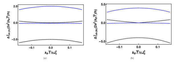
Figure 9: $\Delta^{\eta}_{Tsh(th)}$ vs. $\frac{k_{B}\bar{T}}{cJ^{2}_{0}}$ in unit of $\frac{2e^{2}(k_{B}\bar{T})}{h}$ for (a) setup 1 and (b) setup 2, with shot-noise contributions: $\Delta^{ch}_{Tsh}$ (black, dashed), $\Delta^{sp}_{Tsh}$ (blue, dashed), and thermal noise contributions: $\Delta^{ch}_{Tth}$ (black, dotted), and $\Delta^{sp}_{Tth}$ (blue, dotted).

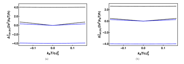
Figure 10: $\Delta^{\eta}_{Tsh(th)}$ vs. $\frac{k_{B}T}{cJ^{2}_{0}}$ in unit of $\frac{2e^{2}(k_{B}T)}{h}$ for (a) setup 3, and (b) setup 4, with shot noise contributions: $\Delta^{ch}_{Tsh}$ (black, dashed), $\Delta^{sp}_{Tsh}$ (blue, dashed), and thermal noise contributions: $\Delta^{ch}_{Tth}$ (black, dotted), and $\Delta^{sp}_{Tth}$ (blue, dotted).

Again for the first time, we have calculated $\Delta^{sp}_{T}$ noise due to spin-flip scattering, which is negative as a function of $\frac{k_{B}T}{cJ^{2}_{0}}$ in setups 3 and 4, whereas it is positive as a function of $\frac{k_{B}\bar{T}}{cJ^{2}_{0}}$ in setups 1 and 2. To our knowledge, spin-polarised $\Delta^{sp}_{T}$, $\Delta^{sp}_{Tth}$ and $\Delta^{sp}_{Tsh}$ noise due to spin-flip scattering, has never been calculated before. However, $\Delta^{sp}_{Tsh}/\Delta^{sp}_{Tth}$ ratio with temperature bias and spin bias (i.e., spin-dependent chemical potential, with spin-independent transmission) in the absence of any spin-flip scattering has been calculated, see Ref. [15], which obeys the general bound, i.e., $\Delta^{sp}_{Tsh}/\Delta^{sp}_{Tth}<1$. Intriguingly, introducing a spin-flipper at the interface of a metallic bilayer junction, as we have done in Fig. 1, leads to $\Delta^{sp}_{T}$ being positive for reservoirs with comparable temperatures, whereas it is negative throughout for one hot and other cold reservoir. For reservoirs with comparable temperatures (in setups 1 and 2), dominant contributions from thermal noise $\Delta^{sp}_{Tth}$ is positive, which leads to positive $\Delta^{sp}_{T}$, whereas shot noise contribution $\Delta^{sp}_{Tsh}$ is negative in the limit of $|\frac{k_{B}\bar{T}}{cJ^{2}_{0}}|<1$, see Fig. 9. On the other hand, in one hot and other cold reservoir case (setups 3 and 4), the contribution from thermal noise denoted as $\Delta^{sp}_{Tth}$, leads to negative $\Delta^{sp}_{T}$ as coefficients of expansion factor $\frac{k_{B}T}{cJ^{2}_{0}}$ are negative, see Eqs (40-42), and Fig. 10. However, the shot noise contribution, denoted as $\Delta^{sp}_{Tsh}$, is positive for setups 3 and 4. Similar to the charge noise $\Delta^{ch}_{T}$, spin noise $\Delta^{sp}_{T}$ also follows the general bound, namely $\mid\frac{\Delta^{sp}_{Tsh}}{\Delta^{sp}_{Tth}}\mid<1$ in each setup. This bound tends to zero around $\frac{k_{B}\bar{T}}{cJ^{2}_{0}}\rightarrow 0$ for reservoirs with comparable temperatures, which indicates $\Delta^{sp}_{Tsh}$ is negligible compared to $\Delta^{sp}_{Tth}$ for $\frac{k_{B}\bar{T}}{cJ^{2}_{0}}\rightarrow 0$. In contrast, it remains finite for one hot and other cold reservoir, around $\frac{k_{B}T}{cJ^{2}_{0}}\rightarrow 0$.

For reservoirs with comparable temperatures (setups 1 and 2), unlike $\Delta^{ch}_{Tsh}$, $\Delta^{sp}_{Tsh}$ noise is negative because no-flip contributions ($\Delta^{\uparrow\uparrow}_{Tsh}$ and $\Delta^{\downarrow\downarrow}_{Tsh}$) are less than spin-flip contributions ($\Delta^{\uparrow\downarrow}_{Tsh}$ and $\Delta^{\downarrow\uparrow}_{Tsh}$). The spin-flip contributions ($\Delta^{\uparrow\downarrow}_{Tth}$ and $\Delta^{\downarrow\uparrow}_{Tth}$) are less than no-flip contributions ($\Delta^{\uparrow\uparrow}_{Tth}$ and $\Delta^{\downarrow\downarrow}_{Tth}$) and positive, consequently, the $\Delta^{sp}_{Tth}$ noise is positive. In case of one hot and other cold reservoir, negative $\Delta^{sp}_{Tth}$ noise arises due to the dominant spin-flip contributions ($\Delta^{\uparrow\downarrow}_{Tth}$, $\Delta^{\downarrow\uparrow}_{Tth}$), and similar to $\Delta^{ch}_{Tsh}$, $\Delta^{sp}_{Tsh}$ noise is positive due to the positive contributions from both no-flip ($\Delta^{\uparrow\uparrow}_{Tsh},\Delta^{\downarrow\downarrow}_{Tsh}$) and spin-flip ($\Delta^{\uparrow\downarrow}_{Tsh},\Delta^{\downarrow\uparrow}_{Tsh}$) contributions.

Below, we compare our results for the N₁/SF/N₂ case with the NIN case when spin-flip scattering is absent. $\Delta_{T}$ noise in the absence of any spin-flip scattering for NIN junction, i.e., $\Delta^{N}_{T}=\Delta^{ch}_{T}=\Delta^{sp}_{T}$ is consistently positive and robust to any change in $\frac{k_{B}\bar{T}}{cJ^{2}_{0}}$ or setups considered. In an earlier work, in a system of two normal metals separated by a quantum dot with temperature bias and zero bias case similar to our setup 1, it has been shown that $\Delta^{N}_{T}$ noise is always positive, see Ref. [14]. Ref. [12] takes voltage and temperature bias configuration values similar to our setup 4. Our results of $\Delta^{N}_{T}$ noise for a NIN junction is in agreement with the results of Ref. [12].

Next, we compare the sign of $\Delta^{N}_{Tsh}$ with some previous works, see Refs. [16, 11, 14, 12, 15] to see the effect of spin-flip scattering in our work. It has been seen that the sign of $\Delta^{N}_{Tsh}$ can probe quantum statistics, i.e., positive for fermions and either positive or negative for bosons  [16]. $\Delta^{N}_{Tsh}=\Delta^{ch}_{Tsh}=\Delta^{sp}_{Tsh}$ is always positive regardless of setups considered. Our results are similar to Ref. [14] wherein the temperature gradient and voltage bias are similar to our setup 1 for a bilayer metallic junction separated by a quantum dot. Our results also agree with Ref. [12] for two generic conductors with temperature and voltage bias similar to setup 4 of our paper. This serves as a consistency check.

Characteristic of the negative signature of $\Delta^{ch}_{T}$ and $\Delta^{sp}_{T}$ noise makes this a valuable tool to measure spin-polarized transport in spintronics by simply changing the temperature bias. Our most important result, i.e., negative charge or spin thermal noise-like contribution to $\Delta^{ch(sp)}_{T}$, i.e., $\Delta^{ch(sp)}_{Tth}$ and negative shot noise-like contribution to spin $\Delta^{sp}_{T}$, i.e., $\Delta^{sp}_{Tsh}$ underline the impact of spin-flip scattering in a bilayer metallic junction.

V Conclusion

Recently, the temperature generated $\Delta_{T}$ quantum noise has been measured for zero charge current along with thermal noise-like contribution and shot noise-like contributions [13, 9, 10]. $\Delta_{T}$ shot noise-like contribution has been calculated by subtracting the thermal noise-like contribution from total $\Delta_{T}$ noise. In Ref. [13], total $\Delta_{T}$ noise is measured in an atomic scale molecular junction using the break junction technique, driven out by temperature gradient bias similar to our setup 1. For temperature-generated noise, $\Delta_{T}$ noise can be calculated for the four setups used in our work by changing the temperature or the voltage bias in an N₁/SF/N₂ junction, and magnetic impurity can be doped at the interface, which acts as a spin-flipper [17].

We have calculated charge $\Delta^{ch}_{T}$ noise and spin $\Delta^{sp}_{T}$ noise with respective contributions from thermal and shot noise-like without charge current and spin current, respectively. Charge $\Delta^{ch}_{T}$ and spin $\Delta^{sp}_{T}$ noise turn negative due to spin-flip scattering as a function of $\frac{k_{B}\bar{T}}{cJ^{2}_{0}}$ depending on the temperature gradient and setups used. $\Delta^{ch}_{Tth}$ is negative, which leads to negative $\Delta^{ch}_{T}$, whereas $\Delta^{ch}_{Tsh}$ is always positive as predicted for fermions. However, $\Delta^{N}_{Tth}$ is always positive for a NIN junction, implying that introducing a spin-flipper at the interface gives negative $\Delta^{ch(sp)}_{T}$ thermal noise-like contribution. Negative $\Delta^{ch}_{Tth}$ noise is seen due to the spin-flip contributions turning negative. Negative $\Delta^{ch}_{Tth}$ noise has also been predicted in Ref. [14]. Focusing on spin noise, $\Delta^{sp}_{Tsh}$ is negative (in setups 1 and 2) that is purely due to spin-flip scattering, unlike charge $\Delta^{ch}_{Tsh}$, which is always positive for fermions. However, for setups 3 and 4, $\Delta^{sp}_{Tsh}$ is positive. We confirm the general bound of $\Delta_{T}$ noise in a NIN junction  [12], i.e., shot noise-like is always less than thermal noise-like contribution ($|\Delta^{N}_{Tsh}/\Delta^{N}_{Tth}|<1$), charge and spin $\Delta_{T}$ noise also follow such a bound irrespective of the temperature gradient or setups used. For reservoirs with comparable temperatures, $|\Delta^{ch}_{Tsh}/\Delta^{ch}_{Tth}|<1$ and $|\Delta^{sp}_{Tsh}/\Delta^{sp}_{Tth}|<1$, and $|\Delta^{ch(sp)}_{Tsh}/\Delta^{ch(sp)}_{Tth}|$ vanish around $\mid\frac{k_{B}\bar{T}}{cJ^{2}_{0}}\mid\rightarrow 0$, whereas these are finite in case of one hot and other cold reservoir around $\mid\frac{k_{B}T}{cJ^{2}_{0}}\mid\rightarrow 0$.

Negative charge $\Delta^{ch}_{T}$ noise and spin $\Delta^{sp}_{T}$ noise arise due to spin-flip scattering in N₁/SF/N₂ junction, whereas $\Delta^{N}_{T}$ noise is always positive in the absence of spin-flip scattering irrespective of the setups used. For the first time, we see spin $\Delta_{T}$ shot noise-like contribution turns negative even for fermions. We expect this signature of negative $\Delta^{ch}_{T}$ noise due to temperature gradient to be useful in studying spin-flip scattering experimentally, $\Delta_{T}$ noise being an adaptable probe.

Appendix

The Appendix consists of three sections. First, in Appendix A, we calculate the thermovoltage in each setup after imposing the vanishing current condition. Next, we derive spin-polarized charge and spin quantum noise in Appendix B. Finally, in section C, we analytically derive charge and spin $\Delta_{T}$ shot noise-like contribution and charge and spin $\Delta_{T}$ thermal noise-like contribution for vanishing charge and spin current respectively, for each setup.

Appendix A Average charge and spin current with finite temperature gradient

The average charge current in normal metal $N_{1}$ is given as,

$$I^{ch}_{1} = \sum_{\sigma\in\{\uparrow,\downarrow\}}\langle I^{\sigma}_{1}\rangle=\frac{e}{h}\int^{\infty}_{-\infty}\sum_{\sigma\in\{\uparrow,\downarrow\}}\sum_{\begin{subarray}{c}\gamma,\gamma^{\prime}\in\{1,2\};\\ \rho,\rho^{\prime}\in\{\uparrow,\downarrow\}\end{subarray}}\langle a^{\rho\dagger}_{\gamma}a^{\rho^{\prime}}_{\gamma^{\prime}}\rangle A^{\rho\rho^{\prime}}_{\gamma^{\prime}\gamma}(1,\sigma,E)dE=\frac{e}{h}\sum_{\sigma\in\{\uparrow,\downarrow\}}\sum_{\begin{subarray}{c}\gamma,\gamma^{\prime}\in\{1,2\};\\ \rho,\rho^{\prime}\in\{\uparrow,\downarrow\}\end{subarray}}\int^{\infty}_{-\infty}dE(\delta_{\gamma 1}\delta_{\gamma^{\prime}1}\delta_{\sigma\rho}\delta_{\sigma\rho^{\prime}}-s^{\sigma\rho\dagger}_{1\gamma}s^{\sigma\rho^{\prime}}_{1\gamma^{\prime}})(\delta_{\gamma\gamma^{\prime}}\delta_{\rho\rho^{\prime}}f_{\gamma})$$ (44)

$$= \frac{e}{h}\int^{\infty}_{-\infty}\biggl{\{}\left(1-s^{\uparrow\uparrow\dagger}_{11}s^{\uparrow\uparrow}_{11}-s^{\uparrow\downarrow\dagger}_{11}s^{\uparrow\downarrow}_{11}+1-s^{\downarrow\uparrow\dagger}_{11}s^{\downarrow\uparrow}_{11}-s^{\downarrow\downarrow\dagger}_{11}s^{\downarrow\downarrow}_{11}\right)f_{1}-\left(s^{\uparrow\uparrow\dagger}_{12}s^{\uparrow\uparrow}_{12}+s^{\uparrow\downarrow\dagger}_{12}s^{\uparrow\downarrow}_{12}+s^{\downarrow\uparrow\dagger}_{12}s^{\downarrow\uparrow}_{12}+s^{\downarrow\downarrow\dagger}_{12}s^{\downarrow\downarrow}_{12}\right)f_{2}\biggr{\}}dE$$

$$= \frac{e}{h}\int^{\infty}_{-\infty}\biggl{\{}\left(1-\mathcal{R}^{\uparrow\uparrow}-\mathcal{R}^{\uparrow\downarrow}+1-\mathcal{R}^{\downarrow\uparrow}-\mathcal{R}^{\downarrow\downarrow}\right)f_{1}-\left(\mathcal{T}^{\uparrow\uparrow}+\mathcal{T}^{\uparrow\downarrow}+\mathcal{T}^{\downarrow\uparrow}+\mathcal{T}^{\downarrow\downarrow}\right)f_{2}\biggr{\}}dE$$

$$= \frac{e}{h}\int^{\infty}_{-\infty}\biggl{\{}\left(\mathcal{T}^{\uparrow\uparrow}+\mathcal{T}^{\uparrow\downarrow}+\mathcal{T}^{\downarrow\uparrow}+\mathcal{T}^{\downarrow\downarrow}\right)(f_{1}-f_{2})\biggr{\}}dE=\frac{e}{h}\int^{\infty}_{-\infty}\biggl{\{}F^{ch}_{I}(f_{1}-f_{2})\biggr{\}}dE,$$

where $F^{ch}_{I}=\left(\mathcal{T}^{\uparrow\uparrow}+\mathcal{T}^{\uparrow\downarrow}+\mathcal{T}^{\downarrow\uparrow}+\mathcal{T}^{\downarrow\downarrow}\right)$, $\mathcal{T}^{\uparrow\uparrow}=|s^{\uparrow\uparrow}_{12}|^{2}=|t^{\uparrow\uparrow}|^{2}$, $\mathcal{T}^{\downarrow\uparrow}=|s^{\downarrow\uparrow}_{12}|^{2}=|t^{\downarrow\uparrow}|^{2}$, $\mathcal{T}^{\uparrow\downarrow}=|s^{\uparrow\downarrow}_{12}|^{2}=|t^{\uparrow\downarrow}|^{2}$, $\mathcal{T}^{\downarrow\downarrow}=|s^{\downarrow\downarrow}_{12}|^{2}=|t^{\downarrow\downarrow}|^{2}$, $\mathcal{R}^{\uparrow\uparrow}=|s^{\uparrow\uparrow}_{11}|^{2}=|r^{\uparrow\uparrow}|^{2}$, $\mathcal{R}^{\downarrow\uparrow}=|s^{\downarrow\uparrow}_{11}|^{2}=|r^{\downarrow\uparrow}|^{2}$, $\mathcal{R}^{\uparrow\downarrow}=|s^{\uparrow\downarrow}_{11}|^{2}=|r^{\uparrow\downarrow}|^{2}$ and $\mathcal{R}^{\downarrow\downarrow}=|s^{\downarrow\downarrow}_{11}|^{2}=|r^{\downarrow\downarrow}|^{2}$. $f_{\gamma}(E)=\left[1+e^{\frac{E}{k_{B}T_{\gamma}}}\right]^{-1}$ is Fermi function in normal metal $\gamma=1,2$, $k_{B}$ is Boltzmann constant and $T_{\gamma}$ is temperature in normal metal $\gamma$.

The average spin current in normal metal $N_{1}$, i.e., $\langle I^{\uparrow}_{1}\rangle-\langle I^{\downarrow}_{1}\rangle$ is then,

$$I^{sp}_{1} = \frac{e}{h}\int^{\infty}_{-\infty}\left(\mathcal{T}^{\uparrow\uparrow}-\mathcal{T}^{\uparrow\downarrow}-\mathcal{T}^{\downarrow\uparrow}+\mathcal{T}^{\downarrow\downarrow}\right)(f_{1}-f_{2})dE=\frac{e}{h}\int^{\infty}_{-\infty}F^{sp}_{I}(f_{1}-f_{2})dE,$$ (45)

where $F^{sp}_{I}=\left(\mathcal{T}^{\uparrow\uparrow}-\mathcal{T}^{\uparrow\downarrow}-\mathcal{T}^{\downarrow\uparrow}+\mathcal{T}^{\downarrow\downarrow}\right)$. For NIN junction, average current is $I^{N}_{1}=I^{ch}_{1}=I^{sp}_{1}=\frac{e}{h}\int^{\infty}_{-\infty}\mathcal{T}^{N}(f_{1}-f_{2})dE=\frac{e}{h}\int^{\infty}_{-\infty}F^{N}_{I}(f_{1}-f_{2})dE$, as without spin-flip scattering $|s^{\downarrow\uparrow}_{12}|^{2}=|s^{\uparrow\downarrow}_{12}|^{2}=0$ and $F^{N}_{I}=\mathcal{T}^{N}=|s^{N}_{12}|^{2}=|s^{\uparrow\uparrow}_{12}|^{2}=|s^{\downarrow\downarrow}_{12}|^{2}$.

A.1 Average charge and spin current in Setup 1

We start by calculating the thermovoltage for setup 1, where $V_{1}=V_{2}=V$ in the zero-bias case. This thermovoltage is denoted as $V$, and $T_{\gamma}$ represents the temperature of the reservoir $\gamma$. We assume that $T_{1}\neq T_{2}\neq 0$, with $\frac{\Delta T}{2\bar{T}}\ll 1$ ($\Delta T=T_{1}-T_{2}$, and $\bar{T}=(T_{1}+T_{2})/2$). The Fermi functions, are defined as $f_{1}=\left[1+e^{\frac{E-V}{k_{B}T_{1}}}\right]^{-1}$ and $f_{2}=\left[1+e^{\frac{E-V}{k_{B}T_{2}}}\right]^{-1}$, where $T_{1}=\bar{T}+\Delta T/2$ and $T_{2}=\bar{T}-\Delta T/2$. We can express $f_{1}(E-V,k_{B}T_{1})$ as $f_{1}(E-V,k_{B}\bar{T}+k_{B}\Delta T/2)$ and $f_{2}(E-V,k_{B}T_{2})$ as $f_{2}(E-V,k_{B}\bar{T}-k_{B}\Delta T/2)$.

To investigate the thermovoltage due to temperature gradient, we expand the Fermi functions in powers of $\frac{\Delta T}{2\bar{T}}$. The Fermi functions in the average current $I^{ch}_{1}$, as given in Eq. (44), can be derived using this expansion

$$f_{1}(E-V,k_{B}T_{1})-f_{2}(E-V,k_{B}T_{2}) = 2k_{B}\bar{T}\frac{\partial f(E-V)}{\partial k_{B}T}\left(\frac{\Delta T}{2\bar{T}}\right)+O\left(\frac{\Delta T}{2\bar{T}}\right)^{3},$$ (46)

where $f(E-V)=1/(1+e^{\frac{E-V}{k_{B}\bar{T}}})$ and $\left.\frac{\partial f(E-V)}{\partial k_{B}T}=\frac{\partial f(E-V)}{\partial k_{B}T}\right|_{T=\bar{T}}$. We adopt the approximation that $\frac{\Delta T}{2\bar{T}}\ll 1$, to simplify the calculation and disregard higher-order terms $O\left(\frac{\Delta T}{2\bar{T}}\right)^{3}$. Scattering term $F^{\eta}_{I}$ are function of $\left(\frac{E}{cJ^{2}_{0}}\right)$. Now average charge current in N₁ is,

$$I^{ch}_{1} = \frac{e}{h}\int^{\infty}_{-\infty}F^{ch}_{I}\left(\frac{E}{cJ^{2}_{0}}\right)\biggl{(}f_{1}-f_{2}\biggr{)}dE=\frac{e}{h}\int^{\infty}_{-\infty}F^{ch}_{I}\left(\frac{E}{cJ^{2}_{0}}\right)2k_{B}\bar{T}\frac{\partial f(E-V)}{\partial k_{B}T}\left(\frac{\Delta T}{2\bar{T}}\right)dE,$$ (47)

where $F^{ch}_{I}\left(\frac{E}{cJ^{2}_{0}}\right)=\mathcal{T}^{\uparrow\uparrow}\left(\frac{E}{cJ^{2}_{0}}\right)+\mathcal{T}^{\uparrow\downarrow}\left(\frac{E}{cJ^{2}_{0}}\right)+\mathcal{T}^{\downarrow\uparrow}\left(\frac{E}{cJ^{2}_{0}}\right)+\mathcal{T}^{\downarrow\downarrow}\left(\frac{E}{cJ^{2}_{0}}\right)$. To simplify the integration, we take $\frac{E}{k_{B}\bar{T}}=\omega$, thus, $F^{ch}_{I}\left(\frac{E}{cJ^{2}_{0}}\right)$ can be rewritten as $F^{ch}_{I}\left(\frac{k_{B}\bar{T}\omega}{cJ^{2}_{0}}\right)$. To evaluate the integral terms, we use a Taylor series expansion of $F^{ch}_{I}\left(\frac{k_{B}\bar{T}\omega}{cJ^{2}_{0}}\right)$ in $\frac{k_{B}\bar{T}\omega}{cJ^{2}_{0}}$. Specifically, we substitute $F^{ch}_{I}\left(\frac{k_{B}\bar{T}\omega}{cJ^{2}_{0}}\right)$ with its Taylor series expansion, $F^{ch}_{I}=\sum^{n=\infty}_{n=0}(F^{ch}_{I}(0))^{(n)}\frac{(k_{B}\bar{T}\omega)^{n}}{n!(cJ^{2}_{0})^{n}}$, where $(F^{ch}_{I})^{n}$ represents the $n$th derivative of $F^{ch}_{I}$ with respect to $\frac{E}{cJ^{2}_{0}}$.

$$I^{ch}_{1} = \frac{2e}{h}(k_{B}\bar{T})^{2}\int^{\infty}_{-\infty}F^{ch}_{I}\left(\frac{k_{B}\bar{T}\omega}{cJ^{2}_{0}}\right)\left(\frac{\partial f(E-V)}{\partial k_{B}T}\right)_{E=k_{B}\bar{T}\omega}\left(\frac{\Delta T}{2\bar{T}}\right)d\omega=\frac{2e(k_{B}\bar{T})^{2}}{h}\sum_{n}\frac{(F^{ch}_{I}(0))^{(n)}}{n!}\int^{\infty}_{-\infty}\left(\frac{k_{B}\bar{T}\omega}{cJ^{2}_{0}}\right)^{n}\left(\frac{\partial f(E-V)}{\partial k_{B}T}\right)_{E=k_{B}\bar{T}\omega}\left(\frac{\Delta T}{2\bar{T}}\right)d\omega$$ (48)

$$= \frac{2e(k_{B}\bar{T})^{2}}{h}\sum_{n}\frac{(F^{ch}_{I}(0))^{(n)}}{n!}\int^{\infty}_{-\infty}\left(\frac{k_{B}\bar{T}\omega}{cJ^{2}_{0}}\right)^{n}\left(\frac{\partial f(E-V)}{\partial k_{B}T}\right)_{E=k_{B}\bar{T}\omega}d\omega\left(\frac{\Delta T}{2\bar{T}}\right)$$

$$= \frac{2e(k_{B}\bar{T})^{2}}{h}\left[F^{ch}_{I}(0)\int^{\infty}_{-\infty}\left(\frac{\partial f(E-V)}{\partial k_{B}T}\right)_{E=k_{B}\bar{T}\omega}d\omega+\left(\frac{k_{B}\bar{T}}{cJ^{2}_{0}}\right)(F^{ch}_{I}(0))^{(1)}\int^{\infty}_{-\infty}\omega\left(\frac{\partial f(E-V)}{\partial k_{B}T}\right)_{E=k_{B}\bar{T}\omega}d\omega+\left(\frac{k_{B}\bar{T}}{cJ^{2}_{0}}\right)^{2}\frac{(F^{ch}_{I}(0))^{(2)}}{2!}\right.$$

$$\left.\int^{\infty}_{-\infty}\omega^{2}\left(\frac{\partial f(E-V)}{\partial k_{B}T}\right)_{E=k_{B}\bar{T}\omega}d\omega+O\left(\frac{k_{B}\bar{T}}{cJ^{2}_{0}}\right)^{3}\right]\left(\frac{\Delta T}{2\bar{T}}\right)$$

We keep up to the second order of $\frac{k_{B}\bar{T}}{cJ^{2}_{0}}$ and neglect higher order $O\left(\frac{k_{B}\bar{T}}{cJ^{2}_{0}}\right)^{3}$ terms, for $\frac{k_{B}\bar{T}}{cJ^{2}_{0}}\ll 1$, which does not impact the thermovoltage results. It is important to note that this approximation depends on the system’s specific setup and may need to be adjusted as changes are made.

$$\text{Now,}\leavevmode\nobreak\ \left.I^{ch}_{1}\right|_{n=0}=0,\leavevmode\nobreak\ \left.I^{ch}_{1}\right|_{n=1}=\frac{2ek_{B}\bar{T}}{h}(F^{ch}_{I}(0))^{(1)}\frac{k_{B}\bar{T}}{cJ^{2}_{0}}\left(\frac{\pi^{2}}{3}\right)\left(\frac{\Delta T}{2\bar{T}}\right),\text{and}\leavevmode\nobreak\ \left.I^{ch}_{1}\right|_{n=2}=\frac{2ek_{B}\bar{T}}{h}\frac{(F^{ch}_{I}(0))^{(2)}}{2!}\left(\frac{k_{B}\bar{T}}{cJ^{2}_{0}}\right)^{2}\left(2\frac{\pi^{2}V}{3k_{B}\bar{T}}\right)\left(\frac{\Delta T}{2\bar{T}}\right),$$ (49)

where $(F^{ch}_{I})^{(1)}$ and $(F^{ch}_{I})^{(2)}$ are the first and second derivatives of $F^{ch}_{I}$ with respect to $\frac{E}{cJ^{2}_{0}}$, respectively. The thermovoltage with temperature and voltage configurations similar to setup 1 has never been calculated.

$$\text{Thus,}\leavevmode\nobreak\ \leavevmode\nobreak\ I^{ch}_{1}= \frac{2ek_{B}\bar{T}}{h}\left[\left(\frac{k_{B}\bar{T}}{cJ^{2}_{0}}\right)(F^{ch}_{I}(0))^{(1)}\frac{\pi^{2}}{3}+\left(\frac{k_{B}\bar{T}}{cJ^{2}_{0}}\right)^{2}\frac{V\pi^{2}}{3k_{B}\bar{T}}(F^{ch}_{I}(0))^{(2)}\right]\left(\frac{\Delta T}{2\bar{T}}\right),$$

Equating $$I^{ch}_{1}=0 (F^{ch}_{I}(0))^{(1)}(cJ^{2}_{0})+(F^{ch}_{I}(0))^{(2)}V=0,\leavevmode\nobreak\ \leavevmode\nobreak\ \text{or}\leavevmode\nobreak\ \left.V\right|_{I^{ch}_{1}=0}=(cJ^{2}_{0})\frac{(F^{ch}_{I}(0))^{(1)}}{(F^{ch}_{I}(0))^{(2)}}.$$, we get, (50)

The thermovoltage for each spin configuration differs, as depicted in Fig. 2. In setup 1, the thermovoltage for vanishing charge current in spin-configuration 1 is denoted as $V^{s1}_{ch1}$, with $F^{ch}_{I}(0)=\mathcal{T}^{\uparrow\uparrow}(0)$. On the other hand, for spin-configuration 2, the thermovoltage is denoted as $V^{s1}_{ch2}$, and $F^{ch}_{I}(0)=\mathcal{T}^{\uparrow\uparrow}(0)+\mathcal{T}^{\uparrow\downarrow}(0)$. For spin-configuration 3, the thermovoltage is denoted as $V^{s1}_{ch3}$, and $F^{ch}_{I}(0)=\mathcal{T}^{\downarrow\downarrow}(0)+\mathcal{T}^{\downarrow\uparrow}(0)$. Finally, in spin-configuration 4, where $F^{ch}_{I}(0)=\mathcal{T}^{\downarrow\downarrow}(0)$, the thermovoltage is denoted as $V^{s1}_{ch4}$. However, for energy-independent transmission, $(F^{ch}_{I}(0))^{(1)}$ and $(F^{ch}_{I}(0))^{(2)}$ terms vanish, implying zero charge current irrespective of voltage and temperature bias.

For vanishing spin current, thermovoltage in setup 1 has a similar expression, with $F^{ch}_{I}$ replaced by $F^{sp}_{I}$, giving,

$$\left.V\right|_{I^{sp}_{1}=0}=(cJ^{2}_{0})\frac{(F^{sp}_{I}(0))^{(1)}}{(F^{sp}_{I}(0))^{(2)}}.$$ (51)

In spin configurations 1 and 4, with no-flip scattering, the thermovoltage for vanishing spin-current is equivalent to the thermovoltage for vanishing charge current. The thermovoltage for vanishing spin current in spin-configuration 1 in setup 1 is denoted as $V^{s1}_{sp1}$, with $F^{sp}_{I}(0)=\mathcal{T}^{\uparrow\uparrow}(0)$. For spin-configuration 2, the thermovoltage is denoted as $V^{s1}_{sp2}$, and $F^{sp}_{I}(0)=\mathcal{T}^{\uparrow\uparrow}(0)-\mathcal{T}^{\uparrow\downarrow}(0)$ with an up-spin electron incident. In spin-configuration 3, the thermovoltage is denoted as $V^{s1}_{sp3}$, and $F^{sp}_{I}(0)=\mathcal{T}^{\downarrow\downarrow}(0)-\mathcal{T}^{\downarrow\uparrow}(0)$. Finally, in spin-configuration 4, with $F^{sp}_{I}(0)=\mathcal{T}^{\downarrow\downarrow}(0)$, the thermovoltage is denoted as $V^{s1}_{sp4}$.

Without spin-flip scattering, for a NIN junction, the thermovoltage at vanishing charge current is $\left.V\right|_{I^{N}_{1}=0}$ is derived as,

$$\left.V\right|_{I^{N}_{1}=0}=(cJ^{2}_{0})\frac{(F^{N}_{I}(0))^{(1)}}{(F^{N}_{I}(0))^{(2)}}.$$ (52)

In the case of NIN junction, only two possible spin configurations exist: spin-configuration 1 and spin-configuration 2, see Fig 2. The transmission amplitudes for both spin configurations are identical, i.e., $F^{N}_{I}(0)=\mathcal{T}^{N}(0)=\mathcal{T}^{\uparrow\uparrow}(0)=\mathcal{T}^{\downarrow\downarrow}(0)$ and the thermovoltage is denoted as $V^{s1}_{N}$. $(F^{\eta}_{I})^{(1)}$ and $(F^{\eta}_{I})^{(2)}$ are the first and second derivatives of $F^{\eta}_{I}$ with respect to $\frac{E}{cJ^{2}_{0}}$, where $\eta=ch,\leavevmode\nobreak\ sp$ or $N$.

A.2 Average charge and spin current in Setup 2

First, we derive the thermovoltage for setup 2, with $V_{1}=0$, $V_{2}=-\mu$, and temperatures $T_{1}\neq T_{2}\neq 0$. Similar as setup 1, we assume $\frac{\Delta T}{2\bar{T}}\ll 1$ ($\Delta T=T_{1}-T_{2}$, and $\bar{T}=(T_{1}+T_{2})/2$). The Fermi functions, are defined as $f_{1}=\left[1+e^{\frac{E}{k_{B}T_{1}}}\right]^{-1}$ and $f_{2}=\left[1+e^{\frac{E+\mu}{k_{B}T_{2}}}\right]^{-1}$, where $T_{1}=\bar{T}+\Delta T/2$ and $T_{2}=\bar{T}-\Delta T/2$. We can express $f_{1}(E,k_{B}T_{1})$ as $f_{1}(E,k_{B}\bar{T}+k_{B}\Delta T/2)$ and $f_{2}(E+\mu,k_{B}T_{2})$ as $f_{2}(E+\mu,k_{B}\bar{T}-k_{B}\Delta T/2)$. Similar to setup 1, to calculate the thermovoltage due to temperature gradient, we expand the Fermi functions in powers of $\frac{\Delta T}{2\bar{T}}$. The Fermi functions in the average current $I^{ch}_{1}$, as given in Eq. (44), can be derived using this expansion

$$f_{1}(E,k_{B}T_{1})-f_{2}(E+\mu,k_{B}T_{2}) = \left.(f(E)-f(E+\mu))\right|_{T=\bar{T}}+k_{B}\bar{T}\left(\frac{\partial f(E)}{\partial k_{B}T}+\frac{\partial f(E+\mu)}{\partial k_{B}T}\right)\left(\frac{\Delta T}{2\bar{T}}\right)+O\left(\frac{\Delta T}{2\bar{T}}\right)^{2},$$ (53)

where $f(E+\mu)=\left[1+e^{\frac{E+\mu}{k_{B}\bar{T}}}\right]^{-1}$ and $\left.\frac{\partial f(E+\mu)}{\partial k_{B}T}=\frac{\partial f(E+\mu)}{\partial k_{B}T}\right|_{T=\bar{T}}$. We adopt the approximation that $\frac{\Delta T}{2\bar{T}}\ll 1$ to simplify the calculation and ensure that the results remain unaffected, disregarding higher-order terms $O\left(\frac{\Delta T}{2\bar{T}}\right)^{2}$. Now average charge current in N₁ is,

$$I^{ch}_{1} = \frac{e}{h}\int^{\infty}_{-\infty}F^{ch}_{I}(E)\biggl{(}(f(E)-f(E+\mu))+k_{B}\bar{T}\left(\frac{\partial f(E)}{\partial k_{B}T}+\frac{\partial f(E+\mu)}{\partial k_{B}T}\right)\left(\frac{\Delta T}{2\bar{T}}\right)\biggr{)}dE=\frac{e}{h}\biggl{(}I_{21}+k_{B}\bar{T}I_{22}\left(\frac{\Delta T}{2\bar{T}}\right)\biggr{)},$$ (54)

where $F^{ch}_{I}\left(\frac{E}{cJ^{2}_{0}}\right)=\mathcal{T}^{\uparrow\uparrow}\left(\frac{E}{cJ^{2}_{0}}\right)+\mathcal{T}^{\uparrow\downarrow}\left(\frac{E}{cJ^{2}_{0}}\right)+\mathcal{T}^{\downarrow\uparrow}\left(\frac{E}{cJ^{2}_{0}}\right)+\mathcal{T}^{\downarrow\downarrow}\left(\frac{E}{cJ^{2}_{0}}\right)$. We decompose $I^{ch}_{1}$ into two integrals, i.e., $I_{21}$ and $I_{22}$. To simplify we take, $\frac{E}{k_{B}\bar{T}}=\omega$, thus, the integrals $I_{21}$ and $I_{22}$ are

$$I_{21} = \int^{\infty}_{-\infty}F^{ch}_{I}\left(\frac{E}{cJ^{2}_{0}}\right)(f(E)-f(E+\mu))dE=k_{B}\bar{T}\int^{\infty}_{-\infty}F^{ch}_{I}\left(\frac{k_{B}\bar{T}\omega}{cJ^{2}_{0}}\right)(f(E)-f(E+\mu))_{E=k_{B}\bar{T}\omega}d\omega$$

$$= k_{B}\bar{T}\sum_{n}\frac{(F^{ch}_{I}(0))^{(n)}}{n!}\int^{\infty}_{-\infty}\left(\frac{k_{B}\bar{T}\omega}{cJ^{2}_{0}}\right)^{n}(f(E)-f(E+\mu))_{E=k_{B}\bar{T}\omega}d\omega,$$

and, $$I_{22}=\int^{\infty}_{-\infty}F^{ch}_{I}\left(\frac{E}{cJ^{2}_{0}}\right)\left(\frac{\partial f(E)}{\partial k_{B}T}+\frac{\partial f(E+\mu)}{\partial k_{B}T}\right)dE=k_{B}\bar{T}\sum_{n}\frac{(F^{ch}_{I}(0))^{(n)}}{n!}\int^{\infty}_{-\infty}\left(\frac{k_{B}\bar{T}\omega}{cJ^{2}_{0}}\right)^{n}\left(\frac{\partial f(E)}{\partial k_{B}T}+\frac{\partial f(E+\mu)}{\partial k_{B}T}\right)_{E=k_{B}\bar{T}\omega}d\omega,$$

We evaluate integrals by taking Taylor series expansion of $F^{ch}_{I}\left(\frac{k_{B}\bar{T}\omega}{cJ^{2}_{0}}\right)$ in $\left(\frac{k_{B}\bar{T}\omega}{cJ^{2}_{0}}\right)$, i.e., $F^{ch}_{I}=\sum^{n=\infty}_{n=0}(F^{ch}_{I}(0))^{(n)}\frac{(k_{B}\bar{T}\omega)^{n}}{n!(cJ^{2}_{0})^{n}}$. Keeping the terms up to the second order of $\left(\frac{k_{B}\bar{T}}{cJ^{2}_{0}}\right)$, integrals are,

$$\left.I_{21}\right|_{n=0} = \mu F^{ch}_{I}(0)),\leavevmode\nobreak\ \leavevmode\nobreak\ \left.I_{21}\right|_{n=1}=-\frac{(\mu)^{2}}{k_{B}\bar{T}}\frac{k_{B}\bar{T}}{cJ^{2}_{0}}\frac{(F^{ch}_{I}(0))^{(1)}}{2},\leavevmode\nobreak\ \left.I_{21}\right|_{n=2}=\mu\left(\frac{k_{B}\bar{T}}{cJ^{2}_{0}}\right)^{2}\frac{(F^{ch}_{I}(0))^{(2)}}{2}\frac{\pi^{2}}{3},$$

$$\left.I_{22}\right|_{n=0} = 0,\leavevmode\nobreak\ \left.I_{22}\right|_{n=1}=(F^{ch}_{I}(0))^{(1)}\frac{2\pi^{2}}{3}\frac{k_{B}\bar{T}}{cJ^{2}_{0}},\leavevmode\nobreak\ \left.I_{22}\right|_{n=2}=-\frac{(F^{ch}_{I}(0))^{(2)}}{2}\frac{2\pi^{2}}{3}\left(\frac{k_{B}\bar{T}}{cJ^{2}_{0}}\right)^{2}\left(\frac{\mu}{k_{B}\bar{T}}\right).$$

$$\text{Thus,}\leavevmode\nobreak\ \leavevmode\nobreak\ \leavevmode\nobreak\ I^{ch}_{1} = \frac{e}{h}\biggl{\{}\mu F^{ch}_{I}(0))+k_{B}\bar{T}(F^{ch}_{I}(0))^{(1)}\frac{k_{B}\bar{T}}{cJ^{2}_{0}}\left(\frac{2\pi^{2}}{3}\frac{\Delta T}{2\bar{T}}-\frac{1}{2}\left(\frac{\mu}{k_{B}\bar{T}}\right)^{2}\right)+k_{B}\bar{T}(F^{ch}_{I}(0))^{(2)}\left(\frac{k_{B}\bar{T}}{cJ^{2}_{0}}\right)^{2}\frac{\pi^{2}}{3}\left(\frac{\mu}{k_{B}\bar{T}}\right)\left(\frac{1}{2}-\frac{\Delta T}{2\bar{T}}\right)\biggr{\}},$$ (55)

where $(F^{ch}_{I})^{(1)}$ is the first-order derivative of $F^{ch}_{I}$ with respect to $\frac{E}{cJ^{2}_{0}}$. However, no previous study has calculated thermovoltage for $\Delta_{T}$ noise with temperature and voltage bias configuration similar to setup 2. Equating $I^{ch}_{1}=0$, we get

$$\mu\left(6(cJ^{2}_{0})^{2}(F^{ch}_{I}(0))^{(1)}+(k_{B}\bar{T})^{2}(F^{ch}_{I}(0))^{(2)}\pi^{2}\left(1-2\frac{\Delta T}{2\bar{T}}\right)\right)-(\mu)^{2}3(F^{ch}_{I}(0))^{(1)}(cJ^{2}_{0})+4\pi^{2}(F^{ch}_{I}(0))^{(1)}(cJ^{2}_{0})(k_{B}\bar{T})^{2}\frac{\Delta T}{2\bar{T}}=0$$ (56)

Equating $I^{ch}_{1}=0$, we get thermovoltage $\mu$, i.e., the voltage bias tuned in such a way as to get vanishing charge current in setup 2, as follows,

$$\left.\mu\right|_{I^{ch}_{1}=0}=\frac{\pi^{2}(F^{ch}_{I}(0))^{(2)}(k_{B}\bar{T})^{2}}{6(cJ^{2}_{0})(F^{ch}_{I}(0))^{(1)}}\left(1-2\frac{\Delta T}{2\bar{T}}\right)\left[1+\sqrt[]{1+3\left(\frac{4cJ^{2}_{0}}{\pi k_{B}\bar{T}}\frac{(F^{ch}_{I}(0))^{(1)}}{(F^{ch}_{I}(0))^{(2)}}\frac{1}{1-(\Delta T/\bar{T})}\right)^{2}\frac{\Delta T}{2\bar{T}}}\right].$$ (57)

Similarly as setup 1, in case of setup 2, the thermovoltage for vanishing charge current in spin-configuration 1 is denoted as $\mu^{s2}_{ch1}$, with $F^{ch}_{I}(0)=\mathcal{T}^{\uparrow\uparrow}(0)$ and for spin-configuration 2, the thermovoltage is $\mu^{s2}_{ch2}$ with $F^{ch}_{I}(0)=\mathcal{T}^{\uparrow\uparrow}(0)+\mathcal{T}^{\uparrow\downarrow}(0)$. For spin-configuration 3, the thermovoltage is $\mu^{s2}_{ch3}$, and $F^{ch}_{I}(0)=\mathcal{T}^{\downarrow\downarrow}(0)+\mathcal{T}^{\downarrow\uparrow}(0)$. Finally, in spin-configuration 4, where $F^{ch}_{I}(0)=\mathcal{T}^{\downarrow\downarrow}(0)$, the thermovoltage is denoted as $\mu^{s2}_{ch4}$.

Similarly, for vanishing spin current, thermovoltage in setup 2 is,

$$\left.\mu\right|_{I^{sp}_{1}=0}=\frac{\pi^{2}(F^{sp}_{I}(0))^{(2)}(k_{B}\bar{T})^{2}}{6(cJ^{2}_{0})(F^{sp}_{I}(0))^{(1)}}\left(1-2\frac{\Delta T}{2\bar{T}}\right)\left[1+\sqrt[]{1+3\left(\frac{4cJ^{2}_{0}}{\pi k_{B}\bar{T}}\frac{(F^{sp}_{I}(0))^{(1)}}{(F^{sp}_{I}(0))^{(2)}}\frac{1}{1-(\Delta T/\bar{T})}\right)^{2}\frac{\Delta T}{2\bar{T}}}\right].$$ (58)

The thermovoltage for vanishing spin current in spin-configuration 1(spin-configuration 2) in setup 2 is denoted as $\mu^{s2}_{sp1}$ ($\mu^{s2}_{sp2}$), with $F^{sp}_{I}(0)=\mathcal{T}^{\uparrow\uparrow}(0)$ ($F^{sp}_{I}(0)=\mathcal{T}^{\uparrow\uparrow}(0)-\mathcal{T}^{\uparrow\downarrow}(0)$). In spin-configuration 3, the thermovoltage is denoted as $\mu^{s2}_{sp3}$, and $F^{sp}_{I}(0)=\mathcal{T}^{\downarrow\downarrow}(0)-\mathcal{T}^{\downarrow\uparrow}(0)$, and in spin-configuration 4, with $F^{sp}_{I}(0)=\mathcal{T}^{\downarrow\downarrow}(0)$, the thermovoltage is denoted as $\mu^{s2}_{sp4}$.

$(F^{sp}_{I})^{(1)}$ and $(F^{sp}_{I})^{(2)}$ are first and second order derivatives of $F^{sp}_{I}$ with respect to $\frac{E}{cJ^{2}_{0}}$. Again similar to the derivation without spin-flip scattering for N₁/SF/N₂, in a NIN junction, thermovoltage $\left.\mu\right|_{I^{N}_{1}=0}$ for setup 2 is derived as,

$$\left.\mu\right|_{I^{N}_{1}=0}=\frac{\pi^{2}(F^{N}_{I}(0))^{(2)}(k_{B}\bar{T})^{2}}{6(cJ^{2}_{0})(F^{N}_{I}(0))^{(1)}}\left(1-2\frac{\Delta T}{2\bar{T}}\right)\left[1+\sqrt[]{1+3\left(\frac{4cJ^{2}_{0}}{\pi k_{B}\bar{T}}\frac{(F^{N}_{I}(0))^{(1)}}{(F^{N}_{I}(0))^{(2)}}\frac{1}{1-(\Delta T/\bar{T})}\right)^{2}\frac{\Delta T}{2\bar{T}}}\right],$$ (59)

where $(F^{N}_{I})^{(1)}$ and $(F^{N}_{I})^{(2)}$ are first and second order derivatives of $F^{N}_{I}$ with respect to $\frac{E}{cJ^{2}_{0}}$. The transmission amplitudes for both spin configurations 1 and 4 are identical, i.e., $F^{N}_{I}(0)=\mathcal{T}^{N}(0)=\mathcal{T}^{\uparrow\uparrow}(0)=\mathcal{T}^{\downarrow\downarrow}(0)$ and the thermovoltage is denoted as $\mu^{s2}_{N}$ in setup 2.

A.3 Average charge and spin current in Setup 3

The thermovoltage for setup 3, with zero bias $\Delta V=0$, i.e., $V_{1}=V_{2}=V$, where $V$ is the thermovoltage $V$ and temperatures of the reservoirs are $T_{1}=T$, $T_{2}=0$. Fermi functions are $f_{1}=\left[1+e^{\frac{E-V}{k_{B}T}}\right]^{-1}$ and $f_{2}=\Theta(-E+V)$. Now, the average charge current in N₁ is,

$$I^{ch}_{1} = \sum_{\sigma\in\uparrow,\downarrow}\frac{e}{h}\int^{\infty}_{-\infty}F^{ch}_{I}\left(\frac{E}{cJ^{2}_{0}}\right)\biggl{(}f_{1}-f_{2}\biggr{)}dE=\frac{e}{h}\int^{\infty}_{-\infty}F^{ch}_{I}\left(\frac{E}{cJ^{2}_{0}}\right)\biggl{(}f_{1}-\Theta(-E+V)\biggr{)}dE$$ (60)

$$= \frac{e}{h}\biggl{(}\int^{\infty}_{-\infty}F^{ch}_{I}\left(\frac{E}{cJ^{2}_{0}}\right)f_{1}dE-\int^{V}_{-\infty}F^{ch}_{I}\left(\frac{E}{cJ^{2}_{0}}\right)dE\biggr{)}=\frac{e}{h}\biggl{(}I_{31}-I_{32}\biggr{)}.$$

with $F^{ch}_{I}\left(\frac{E}{cJ^{2}_{0}}\right)=\mathcal{T}^{\uparrow\uparrow}\left(\frac{E}{cJ^{2}_{0}}\right)+\mathcal{T}^{\uparrow\downarrow}\left(\frac{E}{cJ^{2}_{0}}\right)+\mathcal{T}^{\downarrow\uparrow}\left(\frac{E}{cJ^{2}_{0}}\right)+\mathcal{T}^{\downarrow\downarrow}\left(\frac{E}{cJ^{2}_{0}}\right)$. We have decomposed $I^{ch}_{1}$ into two integral terms, $I_{31}$ and $I_{32}$, and evaluated them separately.

To simplify the integration, we take $\frac{E}{k_{B}T}=\omega$, thus, Fermi function is $f_{1}(E-V)=\left[1+e^{\omega-\frac{V}{k_{B}T}}\right]^{-1}$ and $F^{ch}_{I}\left(\frac{E}{cJ^{2}_{0}}\right)$ is $F^{ch}_{I}\left(\frac{k_{B}T\omega}{cJ^{2}_{0}}\right)$. By substituting $F^{ch}_{I}\left(\frac{k_{B}T\omega}{cJ^{2}_{0}}\right)$ with its Taylor series expansion $F^{ch}_{I}=\sum^{n=\infty}_{n=0}(F^{ch}_{I}(0))^{(n)}\frac{(k_{B}T\omega)^{n}}{n!(cJ^{2}_{0})^{n}}$, we obtain the expression

$$I_{31}=k_{B}T\sum^{n=\infty}_{n=0}\frac{(F^{ch}_{I}(0))^{(n)}}{n!}\int^{\infty}_{-\infty}\left(\frac{k_{B}T\omega}{cJ^{2}_{0}}\right)^{n}f_{1}(E-V)_{|E=k_{B}T\omega}d\omega,\leavevmode\nobreak\ \text{similarly, }\leavevmode\nobreak\ I_{32}=k_{B}T\sum^{n=\infty}_{n=0}\frac{(F^{ch}_{I}(0))^{(n)}}{n!}\int^{V}_{-\infty}\left(\frac{k_{B}T\omega}{cJ^{2}_{0}}\right)^{n}d\omega.$$ (61)

We can neglect higher order terms when the approximation $\frac{k_{B}T}{cJ^{2}_{0}}\ll 1$ holds, not impacting the thermovoltage results. Thus,

$$I_{31} = k_{B}T\sum_{n}\frac{(F^{ch}_{I}(0))^{(n)}}{n!}\left(\frac{k_{B}T}{cJ^{2}_{0}}\right)^{n}\int^{\infty}_{-\infty}\omega^{n}f_{1}(E-V)_{|E=k_{B}T\omega}d\omega=2k_{B}T\log 2F^{ch}_{I}(0)+\frac{k_{B}T}{cJ^{2}_{0}}(F^{ch}_{I}(0))^{(1)}\left(\frac{V^{2}}{k_{B}T}-\frac{2\pi^{2}}{3}k_{B}T\right)$$

$$\text{and,\leavevmode\nobreak\ }I_{32} = \int^{\infty}_{-V}F^{ch}_{I}\left(\frac{-E}{cJ^{2}_{0}}\right)dE=\sum_{n}\frac{(F^{ch}_{I}(0))^{(n)}}{n!}\int^{\infty}_{-V}\left(\frac{-E}{cJ^{2}_{0}}\right)^{n}dE=k_{B}T\sum_{n}\frac{(F^{ch}_{I}(0))^{(n)}}{n!}\left(\frac{-k_{B}T}{cJ^{2}_{0}}\right)^{n}\int^{\infty}_{\frac{-V}{k_{B}T}}\omega^{n}d\omega$$ (62)

$$= k_{B}T\left(F^{ch}_{I}(0)\frac{V}{k_{B}T}-\frac{k_{B}T}{cJ^{2}_{0}}\frac{(F^{ch}_{I}(0))^{(1)}}{2}\left(\frac{V}{k_{B}T}\right)^{2}\right).$$

The thermovoltage for a similar setup has been calculated for the vanishing charge current in Refs.  [12, 15].

$$\text{Thus,}\leavevmode\nobreak\ I^{ch}_{1} = \frac{-e}{h}k_{B}T\Biggl{(}\frac{k_{B}T}{cJ^{2}_{0}}(F^{ch}_{I}(0))^{(1)}\frac{2\pi^{2}}{3}+\left(F^{ch}_{I}(0)\left(2\log 2-\frac{V}{k_{B}T}\right)+\frac{k_{B}T}{cJ^{2}_{0}}\frac{3(F^{ch}_{I}(0))^{(1)}}{2}\left(\frac{V}{k_{B}T}\right)^{2}\right)\Biggr{)}+O\left(\frac{k_{B}T}{cJ^{2}_{0}}\right)^{3},$$

$$= \frac{e}{h}\Biggl{(}(k_{B}T)^{2}(F^{ch}_{I}(0))^{(1)}\frac{2\pi^{2}}{3}-(cJ^{2}_{0})F^{ch}_{I}(0)(V-2\log 2k_{B}T)+\frac{3(F^{ch}_{I}(0))^{(1)}}{2}\left(V\right)^{2}\Biggr{)},$$

Equating $$I^{ch}_{1}=0 3(F^{ch}_{I}(0))^{(1)}(V)^{2}-2(cJ^{2}_{0})F^{ch}_{I}(0)V+4(cJ^{2}_{0})F^{ch}_{I}(0)\log 2k_{B}T+(k_{B}T)^{2}(F^{ch}_{I}(0))^{(1)}\frac{4\pi^{2}}{3}=0$$, we get, (63)

Thus, thermovoltage $V$, which leads to vanishing charge current in setup 3, is,

$$\left.V\right|_{I^{ch}_{1}=0}=(cJ^{2}_{0})\frac{F^{ch}_{I}(0)}{3(F^{ch}_{I}(0))^{(1)}}\Bigg{[}1\pm\sqrt[]{1-\left(\frac{k_{B}T}{cJ^{2}_{0}}\right)^{2}\frac{4\pi^{2}}{3}\left(\frac{(F^{ch}_{I}(0))^{(1)}}{F^{ch}_{I}(0)}\right)^{2}-12\log 2\frac{k_{B}T}{cJ^{2}_{0}}\frac{(F^{ch}_{I}(0))^{(1)}}{F^{ch}_{I}(0)}}\Bigg{]}.$$ (64)

Like other setups, the thermovoltages for vanishing charge current in setup 3 are denoted by $V^{s3}_{ch1}$ for spin-configuration 1, with $F^{ch}_{I}(0)=\mathcal{T}^{\uparrow\uparrow}(0)$; $V^{s3}_{ch2}$ for spin-configuration 2, with $F^{ch}_{I}(0)=\mathcal{T}^{\uparrow\uparrow}(0)+\mathcal{T}^{\uparrow\downarrow}(0)$; $V^{s3}_{ch3}$ for spin-configuration 3, with $F^{ch}_{I}(0)=\mathcal{T}^{\downarrow\downarrow}(0)+\mathcal{T}^{\downarrow\uparrow}(0)$; and $V^{s3}_{ch4}$ for spin-configuration 4, with $F^{ch}_{I}(0)=\mathcal{T}^{\downarrow\downarrow}(0)$.

Similarly, for vanishing spin current, thermovoltage in setup 3 can be calculated by replacing $F^{ch}_{I}$ by $F^{sp}_{I}$, which gives,

$$\left.V\right|_{I^{sp}_{1}=0}=(cJ^{2}_{0})\frac{F^{sp}_{I}(0)}{3(F^{sp}_{I}(0))^{(1)}}\Bigg{[}1\pm\sqrt[]{1-\left(\frac{k_{B}T}{cJ^{2}_{0}}\right)^{2}\frac{4\pi^{2}}{3}\left(\frac{(F^{sp}_{I}(0))^{(1)}}{F^{sp}_{I}(0)}\right)^{2}-12\log 2\frac{k_{B}T}{cJ^{2}_{0}}\frac{(F^{sp}_{I}(0))^{(1)}}{F^{sp}_{I}(0)}}\Bigg{]}.$$ (65)

The thermovoltages for vanishing spin current in setup 3 for spin-configuration 1 (spin-configuration 2) are denoted as $V^{s3}_{sp1}$ ($V^{s3}_{sp2}$), with $F^{sp}_{I}(0)=\mathcal{T}^{\uparrow\uparrow}(0)$ ($F^{sp}_{I}(0)=\mathcal{T}^{\uparrow\uparrow}(0)-\mathcal{T}^{\uparrow\downarrow}(0)$). The thermovoltage in spin-configuration 3 is denoted as $V^{s3}_{sp3}$, with $F^{sp}_{I}(0)=\mathcal{T}^{\downarrow\downarrow}(0)-\mathcal{T}^{\downarrow\uparrow}(0)$, and in spin-configuration 4, with $F^{sp}_{I}(0)=\mathcal{T}^{\downarrow\downarrow}(0)$, the thermovoltage is denoted as $V^{s3}_{sp4}$.

In the absence of spin-flip scattering, for a NIN junction, similarly, the thermovoltage $\left.V\right|_{I^{N}_{1}=0}$ for setup 3 can be derived as,

$$\left.V\right|_{I^{N}_{1}=0}=(cJ^{2}_{0})\frac{F^{N}_{I}(0)}{3(F^{N}_{I}(0))^{(1)}}\Bigg{[}1\pm\sqrt[]{1-\left(\frac{k_{B}T}{cJ^{2}_{0}}\right)^{2}\frac{4\pi^{2}}{3}\left(\frac{(F^{N}_{I}(0))^{(1)}}{F^{N}_{I}(0)}\right)^{2}-12\log 2\frac{k_{B}T}{cJ^{2}_{0}}\frac{(F^{N}_{I}(0))^{(1)}}{F^{N}_{I}(0)}}\Bigg{]},$$ (66)

where $(F^{\eta}_{I})^{(1)}$ is first order derivative of $F^{\eta}_{I}$ with respect to $\frac{E}{cJ^{2}_{0}}$, where $\eta=ch$ denotes charge Eq. (64), $\eta=sp$ denotes spin in Eq. (65) and $\eta=N$ denotes NIN in Eq. (66). The thermovoltage is denoted as $V^{s3}_{N}$ for NIN junction, where the transmission amplitudes for both spin configurations 1 and 4 are the same, i.e., $F^{N}_{I}(0)=\mathcal{T}^{N}(0)=\mathcal{T}^{\uparrow\uparrow}(0)=\mathcal{T}^{\downarrow\downarrow}$(0).

A.4 Average charge and spin current in Setup 4

The thermovoltage for setup 4, with $V_{1}=0$, $V_{2}=-\mu$ and temperatures of reservoirs are $T_{1}=T$, $T_{2}=0$. Fermi functions are $f_{1}=\left[1+e^{\frac{E}{k_{B}T}}\right]^{-1}$, $f_{2}=\Theta(-E-\mu)$. Average charge current in N₁ is,

$$I^{ch}_{1} = \frac{e}{h}\int^{\infty}_{-\infty}F^{ch}_{I}\left(\frac{E}{cJ^{2}_{0}}\right)\biggl{(}f_{1}-\Theta(-E-\mu)\biggr{)}dE=\frac{e}{h}\biggl{(}\int^{\infty}_{-\infty}F^{ch}_{I}\left(\frac{E}{cJ^{2}_{0}}\right)f_{1}dE-\int^{\infty}_{-\infty}F^{ch}_{I}\left(\frac{E}{cJ^{2}_{0}}\right)\Theta(-E-\mu)dE\biggr{)}$$ (67)

$$= =\frac{e}{h}\biggl{(}\int^{\infty}_{-\infty}F^{ch}_{I}\left(\frac{E}{cJ^{2}_{0}}\right)f_{1}dE-\int^{-\mu}_{-\infty}F^{ch}_{I}\left(\frac{E}{cJ^{2}_{0}}\right)dE\biggr{)}=\frac{e}{h}\biggl{(}I_{41}-I_{42}\biggr{)},$$

where $F^{ch}_{I}\left(\frac{E}{cJ^{2}_{0}}\right)=\mathcal{T}^{\uparrow\uparrow}\left(\frac{E}{cJ^{2}_{0}}\right)+\mathcal{T}^{\uparrow\downarrow}\left(\frac{E}{cJ^{2}_{0}}\right)+\mathcal{T}^{\downarrow\uparrow}\left(\frac{E}{cJ^{2}_{0}}\right)+\mathcal{T}^{\downarrow\downarrow}\left(\frac{E}{cJ^{2}_{0}}\right)$. It is worth noting that this approximation relies on the particular configuration of the system and might require modifications as the system evolves. We have decomposed $I^{ch}_{1}$ into two integral terms, $I_{41}$ and $I_{42}$, and evaluated them separately.

To simplify the integration process, we set $\frac{E}{k_{B}T}$ equal to $\omega$, which allows us to express the Fermi function as $f_{1}=\left[1+e^{\omega}\right]^{-1}$. We have used a Taylor series expansion of $F^{ch}_{I}\left(\frac{k_{B}T\omega}{cJ^{2}_{0}}\right)$ to evaluate the integral terms. By substituting $F^{ch}_{I}\left(\frac{k_{B}T\omega}{cJ^{2}_{0}}\right)$ with its Taylor series expansion, i.e., $F^{ch}_{I}\left(\frac{k_{B}T\omega}{cJ^{2}_{0}}\right)=\sum^{n=\infty}_{n=0}(F^{ch}_{I}(0))^{(n)}\frac{(k_{B}T\omega)^{n}}{n!(cJ^{2}_{0})^{n}}$, the integrals can be written as,

$$I_{41} = k_{B}T\sum_{n}\frac{(F^{ch}_{I}(0))^{(n)}}{n!}\left(\frac{k_{B}T}{cJ^{2}_{0}}\right)^{n}\int^{\infty}_{-\infty}\omega^{n}f_{1}(k_{B}T\omega)d\omega=k_{B}T\frac{k_{B}T}{cJ^{2}_{0}}(F^{ch}_{I}(0))^{(1)}\frac{\pi^{2}}{6}.$$ (68)

Similarly, taking the Taylor series expansion of $F^{ch}_{I}$ in $I_{42}$, we get,

$$I_{42} = \int^{-\mu}_{-\infty}F^{ch}_{I}\left(\frac{E}{cJ^{2}_{0}}\right)dE\leavevmode\nobreak\ =\leavevmode\nobreak\ \int^{\infty}_{\mu}F^{ch}_{I}\left(\frac{-E}{cJ^{2}_{0}}\right)dE\leavevmode\nobreak\ =\leavevmode\nobreak\ \sum^{n=\infty}_{n=0}\frac{(F^{ch}_{I}(0))^{(n)}}{n!}\int^{\infty}_{\mu}\left(\frac{-E}{cJ^{2}_{0}}\right)^{n}dE\leavevmode\nobreak\$$ (69)

$$= k_{B}T\sum_{n}\frac{(F^{ch}_{I}(0))^{(n)}}{n!}\left(\frac{-k_{B}T}{cJ^{2}_{0}}\right)^{n}\int^{\infty}_{\frac{\mu}{k_{B}T}}\omega^{n}d\omega=(k_{B}T)\left(-F^{ch}_{I}(0)\frac{\mu}{k_{B}T}+\frac{k_{B}T}{cJ^{2}_{0}}\frac{(F^{ch}_{I}(0))^{(1)}}{2}\left(\frac{\mu}{k_{B}T}\right)^{2}\right).$$

As the approximation $\frac{k_{B}T}{cJ^{2}_{0}}\ll 1$ is valid, we disregard higher order terms without affecting the thermovoltage outcomes.

$$\text{Thus,}\leavevmode\nobreak\ I^{ch}_{1} = \frac{e}{h}k_{B}T\Biggl{(}\frac{k_{B}T}{cJ^{2}_{0}}(F^{ch}_{I}(0))^{(1)}\frac{\pi^{2}}{6}-\left(-F^{ch}_{I}(0)\frac{\mu}{k_{B}T}+\frac{k_{B}T}{cJ^{2}_{0}}\frac{(F^{ch}_{I}(0))^{(1)}}{2}\left(\frac{\mu}{k_{B}T}\right)^{2}\right)\Biggr{)}.$$

Equating $$I^{ch}_{1}=0 (F^{ch}_{I}(0))^{(1)}(\mu)^{2}-2(cJ^{2}_{0})F^{ch}_{I}(0)\mu-(k_{B}T)^{2}(F^{ch}_{I}(0))^{(1)}\frac{\pi^{2}}{3}=0.\leavevmode\nobreak\ \leavevmode\nobreak\ \leavevmode\nobreak\ \leavevmode\nobreak\$$, we get, (70)

Thus, thermovoltage for setup 4 obtained by equating $I^{ch}_{1}=0$, is

$$\left.\mu\right|_{I^{ch}_{1}=0}=cJ^{2}_{0}\frac{F^{ch}_{I}(0)}{(F^{ch}_{I}(0))^{(1)}}\Bigg{[}1\pm\sqrt[]{1+\left(\frac{k_{B}T}{cJ^{2}_{0}}\right)^{2}\frac{\pi^{2}}{3}\left(\frac{(F^{ch}_{I}(0))^{(1)}}{F^{ch}_{I}(0)}\right)^{2}}\Bigg{]}.$$ (71)

Hence, we neglect the higher order of $\frac{k_{B}T}{cJ^{2}_{0}}$ with approximation $\frac{k_{B}T}{cJ^{2}_{0}}\ll 1$ to obtain a simplified thermovoltage and neglect the higher-order terms because it does not affect the thermovoltage. The thermovoltage for setup 4 was calculated for the vanishing charge current in Ref. [12], which aligns with the expression for thermovoltage given in Eq. (71) for setup 4.

The thermovoltages for vanishing charge current in setup 4 are denoted as $\mu^{s4}_{ch1}$, $\mu^{s4}_{ch2}$, $\mu^{s4}_{ch3}$, and $\mu^{s4}_{ch4}$ for spin-configurations 1, 2, 3, and 4, respectively, with corresponding $F^{ch}_{I}(0)$ values as mention in previous setups.

Similarly, for vanishing spin current, thermovoltage in setup 4 is derived as

$$\left.\mu\right|_{I^{sp}_{1}=0}=cJ^{2}_{0}\frac{F^{sp}_{I}(0)}{(F^{sp}_{I}(0))^{(1)}}\Bigg{[}1\pm\sqrt[]{1+\left(\frac{k_{B}T}{cJ^{2}_{0}}\right)^{2}\frac{\pi^{2}}{3}\left(\frac{(F^{sp}_{I}(0))^{(1)}}{F^{sp}_{I}(0)}\right)^{2}}\Bigg{]}.$$ (72)

The thermovoltages for vanishing spin current in setup 4 for vanishing spin current are denoted as $\mu^{s4}_{sp1}$, $\mu^{s4}_{sp2}$, $\mu^{s4}_{sp3}$, and $\mu^{s4}_{sp4}$ for spin-configurations 1, 2, 3, and 4, respectively, with corresponding $F^{sp}_{I}(0)$ values as mention in previous setups.

Finally, for a NIN junction without spin-flip scattering, thermovoltage $\left.\mu\right|_{I^{N}_{1}=0}$ for setup 4 is derived as,

$$\left.\mu\right|_{I^{N}_{1}=0}=cJ^{2}_{0}\frac{F^{N}_{I}(0)}{(F^{N}_{I}(0))^{(1)}}\Bigg{[}1\pm\sqrt[]{1+\left(\frac{k_{B}T}{cJ^{2}_{0}}\right)^{2}\frac{\pi^{2}}{3}\left(\frac{(F^{N}_{I}(0))^{(1)}}{F^{N}_{I}(0)}\right)^{2}}\Bigg{]}.$$ (73)

$(F^{\eta}_{I})^{(1)}$ and $(F^{\eta}_{I})^{(2)}$ are first and second order derivatives of $F^{\eta}_{I}$ with respect to $\frac{E}{cJ^{2}_{0}}$, where $\eta=ch$ denotes charge Eq. (71), $\eta=sp$ denotes spin in Eq. (72) and $\eta=N$ denotes NIN in Eq. (73).

The thermovoltage in setup 4 is denoted as $\mu^{s4}_{N}$, where the transmission amplitudes are identical for spin configurations 1 and 4, with $F^{N}_{I}(0)=\mathcal{T}^{N}(0)=\mathcal{T}^{\uparrow\uparrow}(0)=\mathcal{T}^{\downarrow\downarrow}(0)$.

Appendix B Charge and spin quantum noise

The noise correlation [4, 6] between contacts $\alpha$ and $\beta$ is defined $S_{\alpha\beta}(t-t^{\prime})=\frac{1}{2\pi}\langle\Delta I_{\alpha}(t)\Delta I_{\beta}(t^{\prime})+\Delta I_{\beta}(t^{\prime})\Delta I_{\alpha}(t)\rangle$. Similarly, spin-polarized noise [19] is defined as, $S^{\sigma\sigma^{\prime}}_{\alpha\beta}(t-t^{\prime})=\frac{1}{2\pi}\langle\Delta I^{\sigma}_{\alpha}(t)\Delta I^{\sigma^{\prime}}_{\beta}(t^{\prime})+\Delta I^{\sigma^{\prime}}_{\beta}(t^{\prime})\Delta I^{\sigma}_{\alpha}(t)\rangle$, with $\Delta I^{\sigma}_{\alpha}=I^{\sigma}_{\alpha}-\langle I^{\sigma}_{\alpha}\rangle$, where $I^{\sigma}_{\alpha}$ is current with spin $\sigma=\uparrow,\downarrow$ in lead $\alpha$. The charge shot noise for the charge current, $I^{ch}_{\alpha}=I^{\uparrow}_{\alpha}+I^{\downarrow}_{\alpha}$ is $S^{ch}_{\alpha\beta}=S^{\uparrow\uparrow}_{\alpha\beta}+S^{\uparrow\downarrow}_{\alpha\beta}+S^{\downarrow\uparrow}_{\alpha\beta}+S^{\downarrow\downarrow}_{\alpha\beta}$. The spin-shot noise for the spin current $I^{sp}_{\alpha}=I^{\uparrow}_{\alpha}-I^{\downarrow}_{\alpha}$ is $S^{sp}_{\alpha\beta}=S^{\uparrow\uparrow}_{\alpha\beta}-S^{\uparrow\downarrow}_{\alpha\beta}-S^{\downarrow\uparrow}_{\alpha\beta}+S^{\downarrow\downarrow}_{\alpha\beta}$. Noise at zero frequency, $S^{\sigma\sigma^{\prime}}_{\alpha\beta}$ is derived as,

$$S^{\sigma\sigma^{\prime}}_{\alpha\beta} = \frac{e^{2}}{h}\int^{\infty}_{-\infty}dE\sum_{\gamma\gamma^{\prime}\in{1,2};\rho\rho^{\prime}\in{\uparrow,\downarrow}}\left[\left\{\langle a^{\sigma\dagger}_{\alpha}a^{\sigma^{\prime}}_{\beta}a^{\rho\dagger}_{\gamma}a^{\rho^{\prime}}_{\gamma^{\prime}}\rangle-\langle a^{\sigma\dagger}_{\alpha}a^{\sigma^{\prime}}_{\beta}\rangle\langle a^{\rho\dagger}_{\gamma}a^{\rho^{\prime}}_{\gamma^{\prime}}\rangle\right\}A^{\sigma^{\prime}\sigma}_{\alpha\beta}(\alpha,\sigma)A^{\rho^{\prime}\rho}_{\gamma^{\prime}\gamma}(\beta,\sigma^{\prime})\right.$$ (74)

$$\left.+\left\{\langle a^{\sigma^{\prime}\dagger}_{\beta}a^{\sigma}_{\alpha}a^{\rho^{\prime}\dagger}_{\gamma^{\prime}}a^{\rho}_{\gamma}\rangle-\langle a^{\sigma^{\prime}\dagger}_{\beta}a^{\sigma}_{\alpha}\rangle\langle a^{\rho^{\prime}\dagger}_{\gamma^{\prime}}a^{\rho}_{\gamma}\rangle\right\}A^{\sigma\sigma^{\prime}}_{\beta\alpha}(\beta,\sigma^{\prime})A^{\rho\rho^{\prime}}_{\gamma\gamma^{\prime}}(\alpha,\sigma)\right],$$

where $A^{\rho\rho^{\prime}}_{\gamma^{\prime}\gamma}(\alpha,\sigma)=\delta_{\gamma\alpha}\delta_{\gamma^{\prime}\alpha}\delta_{\sigma\rho}\delta_{\sigma\rho^{\prime}}-s^{\sigma\rho\dagger}_{\alpha\gamma}s^{\sigma\rho^{\prime}}_{\alpha\gamma^{\prime}}$. $\langle a^{\sigma\dagger}_{\alpha}a^{\sigma^{\prime}}_{\beta}\rangle=\delta_{\alpha\beta}\delta_{\sigma\sigma^{\prime}}f^{\sigma}_{\alpha}$, where we have considered the Fermi function to be independent of spin, hence $f^{\sigma}_{\alpha}=f_{\alpha}$, and $\langle a^{\sigma\dagger}_{\alpha}a^{\sigma^{\prime}}_{\beta}a^{\rho\dagger}_{\gamma}a^{\rho^{\prime}}_{\gamma^{\prime}}\rangle-\langle a^{\sigma\dagger}_{\alpha}a^{\sigma^{\prime}}_{\beta}\rangle\langle a^{\rho\dagger}_{\gamma}a^{\rho^{\prime}}_{\gamma^{\prime}}\rangle=\delta_{\alpha\gamma^{\prime}}\delta_{\beta\gamma}\delta_{\sigma\rho^{\prime}}\delta_{\sigma^{\prime}\rho}f_{\beta}(1-f_{\alpha})=f_{\gamma}(1-f_{\gamma^{\prime}})$. Thus,

$$S^{\sigma\sigma^{\prime}}_{\alpha\beta} = \frac{e^{2}}{h}\int^{\infty}_{-\infty}dE\sum_{\gamma\gamma^{\prime}\in{1,2};\rho\rho^{\prime}\in{\uparrow,\downarrow}}\left[A^{\rho\rho^{\prime}}_{\gamma\gamma^{\prime}}(\alpha,\sigma)A^{\rho^{\prime}\rho}_{\gamma^{\prime}\gamma}(\beta,\sigma^{\prime})\left\{f_{\gamma}(1-f_{\gamma^{\prime}})+f_{\gamma^{\prime}}(1-f_{\gamma})\right\}\right]$$ (75)

$$= \frac{e^{2}}{h}\int^{\infty}_{-\infty}dE\sum_{\gamma\gamma^{\prime}\in{1,2};\rho\rho^{\prime}\in{\uparrow,\downarrow}}\left[\left(\delta_{\gamma\alpha}\delta_{\gamma^{\prime}\alpha}\delta_{\sigma\rho}\delta_{\sigma\rho^{\prime}}-s^{\sigma\rho\dagger}_{\alpha\gamma}s^{\sigma\rho^{\prime}}_{\alpha\gamma^{\prime}}\right)\left(\delta_{\gamma^{\prime}\beta}\delta_{\gamma\beta}\delta_{\sigma^{\prime}\rho^{\prime}}\delta_{\sigma^{\prime}\rho}-s^{\sigma^{\prime}\rho^{\prime}\dagger}_{\beta\gamma^{\prime}}s^{\sigma^{\prime}\rho}_{\beta\gamma}\right)\left\{f_{\gamma}(1-f_{\gamma^{\prime}})+f_{\gamma^{\prime}}(1-f_{\gamma})\right\}\right].\leavevmode\nobreak\ \leavevmode\nobreak\ \leavevmode\nobreak\$$

Noise auto-correlation $S^{\sigma\sigma^{\prime}}_{11}$ is derived as,

$$S^{\sigma\sigma^{\prime}}_{11} = \frac{e^{2}}{h}\int^{\infty}_{-\infty}dE\sum_{\gamma\gamma^{\prime}\in{1,2};\rho\rho^{\prime}\in{\uparrow,\downarrow}}\left[\left(\delta_{\gamma 1}\delta_{\gamma^{\prime}1}\delta_{\sigma\rho}\delta_{\sigma\rho^{\prime}}-s^{\sigma\rho\dagger}_{1\gamma}s^{\sigma\rho^{\prime}}_{1\gamma^{\prime}}\right)\left(\delta_{\gamma^{\prime}1}\delta_{\gamma 1}\delta_{\sigma^{\prime}\rho^{\prime}}\delta_{\sigma^{\prime}\rho}-s^{\sigma^{\prime}\rho^{\prime}\dagger}_{1\gamma^{\prime}}s^{\sigma^{\prime}\rho}_{1\gamma}\right)\left\{f_{\gamma}(1-f_{\gamma^{\prime}})+f_{\gamma^{\prime}}(1-f_{\gamma})\right\}\right]$$ (76)

$$= \frac{e^{2}}{h}\int^{\infty}_{-\infty}dE\sum_{\rho\rho^{\prime}\in{\uparrow,\downarrow}}\left[\left\{\left(\delta_{11}\delta_{11}\delta_{\sigma\rho}\delta_{\sigma\rho^{\prime}}-s^{\sigma\rho\dagger}_{11}s^{\sigma\rho^{\prime}}_{11}\right)\left(\delta_{11}\delta_{11}\delta_{\sigma^{\prime}\rho^{\prime}}\delta_{\sigma^{\prime}\rho}-s^{\sigma^{\prime}\rho^{\prime}\dagger}_{11}s^{\sigma^{\prime}\rho}_{11}\right)f_{1}(1-f_{1})\right\}+\left\{\left(\delta_{21}\delta_{21}\delta_{\sigma\rho}\delta_{\sigma\rho^{\prime}}-s^{\sigma\rho\dagger}_{12}s^{\sigma\rho^{\prime}}_{12}\right)\right.\right.$$

$$\left.\left.\left(\delta_{21}\delta_{21}\delta_{\sigma^{\prime}\rho^{\prime}}\delta_{\sigma^{\prime}\rho}-s^{\sigma^{\prime}\rho^{\prime}\dagger}_{12}s^{\sigma^{\prime}\rho}_{12}\right)f_{2}(1-f_{2})\right\}+\left\{\left(\delta_{11}\delta_{21}\delta_{\sigma\rho}\delta_{\sigma\rho^{\prime}}-s^{\sigma\rho\dagger}_{11}s^{\sigma\rho^{\prime}}_{12}\right)\left(\delta_{21}\delta_{11}\delta_{\sigma^{\prime}\rho^{\prime}}\delta_{\sigma^{\prime}\rho}-s^{\sigma^{\prime}\rho^{\prime}\dagger}_{12}s^{\sigma^{\prime}\rho}_{11}\right)\right.\right.$$

$$\left.\left.+\left(\delta_{21}\delta_{11}\delta_{\sigma\rho}\delta_{\sigma\rho^{\prime}}-s^{\sigma\rho\dagger}_{12}s^{\sigma\rho^{\prime}}_{11}\right)\left(\delta_{11}\delta_{21}\delta_{\sigma^{\prime}\rho^{\prime}}\delta_{\sigma^{\prime}\rho}-s^{\sigma^{\prime}\rho^{\prime}\dagger}_{11}s^{\sigma^{\prime}\rho}_{12}\right)\right\}\left(f_{1}-f_{2}\right)^{2}\right],$$

where terms with Fermi function coefficients $f_{1}(1-f_{1})$ and $f_{2}(1-f_{2})$ correspond to thermal noise, which is the equilibrium noise contribution to quantum noise. However, the terms with $(f_{1}-f_{2})^{2}$ correspond to the non-equilibrium shot noise that vanishes at equilibrium. The spin contribution to the quantum noise, $S^{\sigma\sigma^{\prime}}_{11}$ given in Eq. (76) can be decomposed into thermal noise ($S^{\sigma\sigma^{\prime}}_{11th}$) and shot noise ($S^{\sigma\sigma^{\prime}}_{11sh}$). Charge shot noise auto-correlation is $S^{ch}_{11sh}=S^{\uparrow\uparrow}_{11sh}+S^{\uparrow\downarrow}_{11sh}+S^{\downarrow\uparrow}_{11sh}+S^{\downarrow\downarrow}_{11sh}$. Shot noise auto-correlation for the different spin-dependent contributions can be derived from Eq. (76) as

$$S^{\uparrow\uparrow}_{11sh} = \frac{2e^{2}}{h}\int^{\infty}_{-\infty}dE\left[\left\{|s^{\uparrow\uparrow}_{12}|^{2}|s^{\uparrow\uparrow}_{11}|^{2}+2Re[s^{\uparrow\uparrow\dagger}_{11}s^{\uparrow\downarrow}_{12}s^{\uparrow\uparrow\dagger}_{12}s^{\uparrow\downarrow}_{11}]+|s^{\uparrow\downarrow}_{12}|^{2}|s^{\uparrow\downarrow}_{11}|^{2}\right\}\left(f_{1}-f_{2}\right)^{2}\right]=\frac{2e^{2}}{h}\int^{\infty}_{-\infty}F^{\uparrow\uparrow}_{11sh}\left(f_{1}-f_{2}\right)^{2}dE,$$

$$S^{\uparrow\downarrow}_{11sh} = \frac{2e^{2}}{h}\int^{\infty}_{-\infty}dE\left[\left\{2Re[s^{\uparrow\downarrow\dagger}_{11}s^{\uparrow\uparrow}_{12}s^{\downarrow\downarrow\dagger}_{12}s^{\downarrow\uparrow}_{11}]+2Re[s^{\uparrow\uparrow\dagger}_{11}s^{\uparrow\downarrow}_{12}s^{\downarrow\downarrow\dagger}_{12}s^{\downarrow\uparrow}_{11}]+2Re[s^{\uparrow\uparrow\dagger}_{12}s^{\uparrow\downarrow}_{11}s^{\downarrow\downarrow\dagger}_{11}s^{\downarrow\uparrow}_{12}]+2Re[s^{\uparrow\downarrow\dagger}_{11}s^{\uparrow\downarrow}_{12}s^{\downarrow\uparrow\dagger}_{12}s^{\downarrow\uparrow}_{11}]\right\}\left(f_{1}-f_{2}\right)^{2}\right]$$

$$= \frac{2e^{2}}{h}\int^{\infty}_{-\infty}F^{\uparrow\downarrow}_{11sh}\left(f_{1}-f_{2}\right)^{2}dE,$$

$$S^{\downarrow\uparrow}_{11sh} = \frac{2e^{2}}{h}\int^{\infty}_{-\infty}dE\left[\left\{2Re[s^{\downarrow\uparrow\dagger}_{11}s^{\downarrow\downarrow}_{12}s^{\uparrow\uparrow\dagger}_{12}s^{\uparrow\downarrow}_{11}]+2Re[s^{\downarrow\downarrow\dagger}_{11}s^{\downarrow\uparrow}_{12}s^{\uparrow\uparrow\dagger}_{12}s^{\uparrow\downarrow}_{11}]+2Re[s^{\downarrow\downarrow\dagger}_{12}s^{\downarrow\uparrow}_{11}s^{\uparrow\uparrow\dagger}_{11}s^{\uparrow\downarrow}_{12}]+2Re[s^{\downarrow\uparrow\dagger}_{11}s^{\downarrow\uparrow}_{12}s^{\uparrow\downarrow\dagger}_{12}s^{\uparrow\downarrow}_{11}]\right\}\left(f_{1}-f_{2}\right)^{2}\right]$$

$$= \frac{2e^{2}}{h}\int^{\infty}_{-\infty}F^{\downarrow\uparrow}_{11sh}\left(f_{1}-f_{2}\right)^{2}dE,$$

$$S^{\downarrow\downarrow}_{11sh} = \frac{2e^{2}}{h}\int^{\infty}_{-\infty}dE\left[\left\{|s^{\downarrow\downarrow}_{12}|^{2}|s^{\downarrow\downarrow}_{11}|^{2}+2Re[s^{\downarrow\downarrow\dagger}_{11}s^{\downarrow\uparrow}_{12}s^{\downarrow\downarrow\dagger}_{12}s^{\downarrow\uparrow}_{11}]+|s^{\downarrow\uparrow}_{12}|^{2}|s^{\downarrow\uparrow}_{12}|^{2}\right\}\left(f_{1}-f_{2}\right)^{2}\right]=\frac{2e^{2}}{h}\int^{\infty}_{-\infty}F^{\downarrow\downarrow}_{11sh}\left(f_{1}-f_{2}\right)^{2}dE.$$ (77)

Charge thermal noise correlations are $S^{ch}_{11th}=S^{\uparrow\uparrow}_{11th}+S^{\uparrow\downarrow}_{11th}+S^{\downarrow\uparrow}_{11th}+S^{\downarrow\downarrow}_{11th}$, and the spin-dependent contributions are derived from Eq. (76) as,

$$S^{\uparrow\uparrow}_{11th} = \frac{2e^{2}}{h}\int^{\infty}_{-\infty}dE\left[\left\{|s^{\uparrow\uparrow}_{12}|^{2}|s^{\downarrow\downarrow}_{12}|^{2}+2Re[s^{\uparrow\uparrow\dagger}_{11}s^{\uparrow\downarrow}_{12}s^{\uparrow\uparrow\dagger}_{11}s^{\uparrow\downarrow}_{11}]+|s^{\uparrow\downarrow}_{11}|^{2}|s^{\downarrow\uparrow}_{11}|^{2}\right\}\left(f_{1}(1-f_{1})+f_{2}(1-f_{2})\right)\right]$$

$$= \frac{2e^{2}}{h}\int^{\infty}_{-\infty}F^{\uparrow\uparrow}_{11th}\left(f_{1}(1-f_{1})+f_{2}(1-f_{2})\right)dE,$$

$$S^{\uparrow\downarrow}_{11th} = \frac{2e^{2}}{h}\int^{\infty}_{-\infty}dE\left[\left\{(1-|s^{\uparrow\downarrow}_{11}|^{2})(1-|s^{\downarrow\uparrow}_{11}|^{2})+2Re[s^{\uparrow\uparrow\dagger}_{11}s^{\uparrow\downarrow}_{11}s^{\downarrow\downarrow\dagger}_{11}s^{\downarrow\uparrow}_{11}]+|s^{\downarrow\uparrow\dagger}_{11}|^{2}|s^{\uparrow\downarrow}_{11}|^{2}\right\}\left(f_{1}(1-f_{1})+f_{2}(1-f_{2})\right)\right]$$

$$= \frac{2e^{2}}{h}\int^{\infty}_{-\infty}F^{\uparrow\uparrow}_{11th}\left(f_{1}(1-f_{1})+f_{2}(1-f_{2})\right)dE,$$

$$S^{\downarrow\uparrow}_{11th} = \frac{2e^{2}}{h}\int^{\infty}_{-\infty}dE\left[\left\{(1-|s^{\downarrow\uparrow}_{11}|^{2})(1-|s^{\uparrow\downarrow}_{11}|^{2})+2Re[s^{\downarrow\downarrow\dagger}_{11}s^{\downarrow\uparrow}_{11}s^{\uparrow\uparrow\dagger}_{11}s^{\uparrow\downarrow}_{11}]+|s^{\uparrow\downarrow\dagger}_{11}|^{2}|s^{\downarrow\uparrow}_{11}|^{2}\right\}\left(f_{1}(1-f_{1})+f_{2}(1-f_{2})\right)\right]$$

$$= \frac{2e^{2}}{h}\int^{\infty}_{-\infty}F^{\downarrow\uparrow}_{11th}\left(f_{1}(1-f_{1})+f_{2}(1-f_{2})\right)dE,$$

$$S^{\downarrow\downarrow}_{11th} = \frac{2e^{2}}{h}\int^{\infty}_{-\infty}dE\left[\left\{|s^{\downarrow\downarrow}_{12}|^{2}|s^{\uparrow\uparrow}_{12}|^{2}+2Re[s^{\downarrow\downarrow\dagger}_{11}s^{\downarrow\uparrow}_{12}s^{\downarrow\downarrow\dagger}_{11}s^{\downarrow\uparrow}_{11}]+|s^{\downarrow\uparrow}_{11}|^{2}|s^{\uparrow\downarrow}_{11}|^{2}\right\}\left(f_{1}(1-f_{2})+f_{2}(1-f_{1})\right)\right]$$ (78)

$$= \frac{2e^{2}}{h}\int^{\infty}_{-\infty}F^{\downarrow\downarrow}_{11th}\left(f_{1}(1-f_{1})+f_{2}(1-f_{2})\right)dE,$$

where $F^{ch}_{11sh}=F^{\uparrow\uparrow}_{11sh}+F^{\uparrow\downarrow}_{11sh}+F^{\downarrow\uparrow}_{11sh}+F^{\downarrow\downarrow}_{11sh}$, and $F^{ch}_{11th}=F^{\uparrow\uparrow}_{11th}+F^{\uparrow\downarrow}_{11th}+F^{\downarrow\uparrow}_{11th}+F^{\downarrow\downarrow}_{11th}$. Total spin shot noise auto-correlation is $S^{sp}_{11sh}=S^{\uparrow\uparrow}_{11sh}-S^{\uparrow\downarrow}_{11sh}-S^{\downarrow\uparrow}_{11sh}+S^{\downarrow\downarrow}_{11sh}$ and spin thermal noise correlations is $S^{sp}_{11th}=S^{\uparrow\uparrow}_{11th}-S^{\uparrow\downarrow}_{11th}-S^{\downarrow\uparrow}_{11th}+S^{\downarrow\downarrow}_{11th}$. Similarly, as charge noise scattering terms for spin noise can be written as $F^{sp}_{11sh}=F^{\uparrow\uparrow}_{11sh}-F^{\uparrow\downarrow}_{11sh}-F^{\downarrow\uparrow}_{11sh}+F^{\downarrow\downarrow}_{11sh}$, and $F^{sp}_{11th}=F^{\uparrow\uparrow}_{11th}-F^{\uparrow\downarrow}_{11th}-F^{\downarrow\uparrow}_{11th}+F^{\downarrow\downarrow}_{11th}$.

For NIN junction, without spin-flip scattering, charge quantum noise is identical to spin quantum noise. For shot noise-like contribution $S^{N}_{11sh}=S^{\uparrow\uparrow}_{11sh}=S^{\downarrow\downarrow}_{11sh}$ as $S^{\downarrow\uparrow}_{11sh}=S^{\uparrow\downarrow}_{11sh}=0$ and thermal noise-like contribution $S^{N}_{11th}=S^{\uparrow\uparrow}_{11th}=S^{\downarrow\downarrow}_{11th}$ as $S^{\downarrow\uparrow}_{11th}=S^{\uparrow\downarrow}_{11th}=0$, implying quantum noise to be $S^{N}_{11}=S^{N}_{11th}+S^{N}_{11sh}$.

$$\text{Thus,}\leavevmode\nobreak\ \leavevmode\nobreak\ S^{N}_{11sh} = \frac{2e^{2}}{h}\int^{\infty}_{-\infty}dE\left[\left\{|s^{N}_{12}|^{2}|s^{N}_{11}|^{2}\right\}\left(f_{1}-f_{2}\right)^{2}\right]=\frac{2e^{2}}{h}\int^{\infty}_{-\infty}F^{N}_{11sh}\left(f_{1}-f_{2}\right)^{2}dE,$$

$$\text{and}\leavevmode\nobreak\ \leavevmode\nobreak\ S^{N}_{11th} = \frac{2e^{2}}{h}\int^{\infty}_{-\infty}dE\left[\left\{|s^{N}_{12}|^{2}|s^{N}_{12}|^{2}\right\}\left(f_{1}(1-f_{1})+f_{2}(1-f_{2})\right)\right]=\frac{2e^{2}}{h}\int^{\infty}_{-\infty}F^{N}_{11th}\left(f_{1}(1-f_{1})+f_{2}(1-f_{2})\right)dE,$$ (79)

where $F^{N}_{11sh}=F^{\uparrow\uparrow}_{11sh}=F^{\downarrow\downarrow}_{11sh}=|s^{N}_{12}|^{2}|s^{N}_{11}|^{2}$ and $F^{N}_{11th}=F^{\uparrow\uparrow}_{11th}=F^{\downarrow\downarrow}_{11th}=|s^{N}_{12}|^{2}|s^{N}_{12}|^{2}$, as $F^{\uparrow\downarrow}_{11sh}=F^{\downarrow\uparrow}_{11sh}=0$ and $F^{\uparrow\downarrow}_{11th}=F^{\downarrow\uparrow}_{11th}=0$ without any spin-flip scattering. In earlier studies, $\Delta_{T}$ auto-correlations have been studied in Refs.  [14, 12, 15] without spin-flip scattering. Here, we focus on $\Delta_{T}$ noise auto-correlations to study the spin transport for the first time.

Appendix C Charge and spin $\Delta_{T}$ noise with shot noise-like ($\Delta^{ch}_{Tsh}$, $\Delta^{sp}_{Tsh}$) and thermal noise-like ($\Delta^{ch}_{Tth}$, $\Delta^{sp}_{Tth}$) contributions

C.1 $\Delta^{ch}_{T}$, $\Delta^{sp}_{T}$ and $\Delta^{N}_{T}$ noise in Setup 1

Next, we calculate the charge $\Delta_{T}$ noise and spin $\Delta_{T}$ noise in setup 1, with $\frac{\Delta T}{2\bar{T}}\ll 1$ ($\Delta T=T_{1}-T_{2}$ and $\bar{T}=(T_{1}+T_{2})/2$) and the zero-bias case $\Delta V=0$, $V_{1}=V_{2}=V$. Fermi functions are $f_{1}(E-V)=1/(1+e^{\frac{E-V}{k_{B}T_{1}}})$ and $f_{2}(E-V)=1/(1+e^{\frac{E-V}{k_{B}T_{2}}})$, as $T_{1}=\bar{T}+\Delta T/2$, $T_{2}=\bar{T}-\Delta T/2$, $f_{1}(E-V,k_{B}T_{1})=f_{1}(E-V,k_{B}\bar{T}+k_{B}\Delta T/2)$, and $f_{2}(E-V,k_{B}T_{2})=f_{2}(E-V,k_{B}\bar{T}-k_{B}\Delta T/2)$.

The charge $\Delta^{ch}_{T}$ noise is derived from the quantum noise, as given in Eq. (76) with a temperature gradient and zero-bias voltage for setup 1. Furthermore, we can decompose $\Delta_{T}$ noise into shot noise-like and thermal noise-like contributions, i.e., $\Delta^{ch}_{T}=\Delta^{ch}_{Tsh}+\Delta^{ch}_{Tth}$. Shot noise given in Eq. (77) leads to $\Delta^{ch}_{Tsh}$ shot noise-like contribution to $\Delta^{ch}_{T}$ noise. We expand in powers of $\frac{\Delta T}{2\bar{T}}$, which is a useful tool for investigating the impact of temperature gradient on $\Delta_{T}$ noise. The Fermi functions in $\Delta_{T}$ shot noise-like contribution are derived as-

$$(f_{1}(E-V,k_{B}T_{1})-f_{2}(E-V,k_{B}T_{2}))^{2} = 4\left(\frac{\partial f(E-V)}{\partial k_{B}T}\right)^{2}\left(\frac{k_{B}\Delta T}{2}\right)^{2}+\frac{4}{3!}\left(\frac{\partial^{3}f(E-V)}{\partial(k_{B}T)^{3}}\right)^{2}\left(\frac{k_{B}\Delta T}{2}\right)^{6}+2\frac{4}{3!}\frac{\partial f(E-V)}{\partial k_{B}T}\frac{\partial^{3}f(E-V)}{\partial(k_{B}T)^{3}}\left(\frac{k_{B}\Delta T}{2}\right)^{4}$$ (80)

$$= 4\left(k_{B}\bar{T}\frac{\partial f(E-V)}{\partial k_{B}T}\right)^{2}\left(\frac{\Delta T}{2\bar{T}}\right)^{2}+\frac{4}{3}\left(k_{B}\bar{T}\right)^{4}\frac{\partial f(E-V)}{\partial k_{B}T}\frac{\partial^{3}f(E-V)}{\partial(k_{B}T)^{3}}\left(\frac{\Delta T}{2\bar{T}}\right)^{4}+O\left(\frac{\Delta T}{2\bar{T}}\right)^{6},$$

where, $f(E-V)=1/(1+e^{\frac{E-V}{k_{B}\bar{T}}})$ and $\left.\frac{\partial f(E-V)}{\partial k_{B}T}=\frac{\partial f(E-V)}{\partial k_{B}T}\right|_{T=\bar{T}}$.

We adopt the approximation that $\frac{\Delta T}{2\bar{T}}\ll 1$, and to simplify the calculation and ensure that the results remain unaffected, we include terms up to $\left(\frac{\Delta T}{2\bar{T}}\right)^{4}$, while disregarding higher-order terms $O\left(\frac{\Delta T}{2\bar{T}}\right)^{6}$. $F^{ch}_{11sh}\left(\frac{E}{cJ^{2}_{0}}\right)f(E-V)$ can alternatively be expressed in terms of $F^{ch}_{11sh}\left(\frac{E+V}{cJ^{2}_{0}}\right)f(E)$. As mentioned in Appendix A, we consider $E=k_{B}\bar{T}\omega$. Charge $\Delta_{T}$ shot noise-like contribution can be then derived as

$$\Delta^{ch}_{Tsh} = \frac{2e^{2}}{h}\int^{\infty}_{-\infty}F^{ch}_{11sh}\left(\frac{E}{cJ^{2}_{0}}\right)(f_{1}(E-V,k_{B}T_{1})-f_{2}(E-V,k_{B}T_{2}))^{2}dE$$

$$= \frac{2e^{2}}{h}k_{B}\bar{T}\int^{\infty}_{-\infty}F^{ch}_{11sh}\left(\frac{k_{B}\bar{T}\omega}{cJ^{2}_{0}}\right)\biggl{\{}4\left(k_{B}\bar{T}\frac{\partial f(E-V)}{\partial k_{B}T}\right)^{2}_{E=k_{B}\bar{T}\omega}\left(\frac{\Delta T}{2\bar{T}}\right)^{2}+\frac{4}{3}\left(k_{B}\bar{T}\right)^{4}\left(\frac{\partial f(E-V)}{\partial k_{B}T}\frac{\partial^{3}f(E-V)}{\partial(k_{B}T)^{3}}\right)_{E=k_{B}\bar{T}\omega}\left(\frac{\Delta T}{2\bar{T}}\right)^{4}\biggr{\}}d\omega$$

We have used a Taylor series expansion of $F^{ch}_{11sh}\left(\frac{k_{B}\bar{T}\omega+V}{cJ^{2}_{0}}\right)$ in $\frac{k_{B}\bar{T}\omega+V}{cJ^{2}_{0}}$ to evaluate the integral terms, i.e., $F^{ch}_{11sh}\left(\frac{k_{B}\bar{T}\omega+V}{cJ^{2}_{0}}\right)=\sum^{n=\infty}_{n=0}\left(F^{ch}_{11sh}\left(\frac{V}{cJ^{2}_{0}}\right)\right)^{(n)}\frac{(k_{B}\bar{T}\omega)^{n}}{n!(cJ^{2}_{0})^{n}}$.

$$= \frac{2e^{2}}{h}k_{B}\bar{T}\left\{4(k_{B}\bar{T})^{2}\sum_{n}\frac{(F^{ch}_{11sh}\left(\frac{V}{cJ^{2}_{0}}\right))^{(n)}}{n!}\left(\frac{k_{B}\bar{T}}{cJ^{2}_{0}}\right)^{n}\int^{\infty}_{-\infty}\omega^{n}\left(\frac{\partial f(E)}{\partial k_{B}T}\right)^{2}_{E=k_{B}\bar{T}\omega}d\omega\left(\frac{\Delta T}{2\bar{T}}\right)^{2}\right.$$ (81)

$$\left.+\frac{4(k_{B}\bar{T})^{4}}{3}\left(\frac{k_{B}\bar{T}}{cJ^{2}_{0}}\right)^{n}\sum_{n}\frac{(F^{ch}_{11sh}\left(\frac{V}{cJ^{2}_{0}}\right))^{(n)}}{n!}\int^{\infty}_{-\infty}\omega^{n}\left(\frac{\partial f(E)}{\partial k_{B}T}\frac{\partial^{3}f(E)}{\partial(k_{B}T)^{3}}\right)_{E=k_{B}\bar{T}\omega}d\omega\left(\frac{\Delta T}{2\bar{T}}\right)^{4}\right\}$$

$$= \frac{2e^{2}}{h}k_{B}\bar{T}\left\{4Ds_{11}\left(\frac{\Delta T}{2\bar{T}}\right)^{2}+\frac{4}{3}Ds_{12}\left(\frac{\Delta T}{2\bar{T}}\right)^{4}\right\}.$$

Following the approximation, $\frac{k_{B}\bar{T}}{cJ^{2}_{0}}\ll 1$, we keep the terms up to the order of $O\left(\frac{k_{B}\bar{T}}{cJ^{2}_{0}}\right)^{2}$ and ignore the higher order terms. Hence integrals can be derived by hand or by Mathematica as

$$Ds_{11} = (k_{B}\bar{T})^{2}\sum_{n}\frac{(F^{ch}_{11sh}\left(\frac{V}{cJ^{2}_{0}}\right))^{(n)}}{n!}\left(\frac{k_{B}\bar{T}}{cJ^{2}_{0}}\right)^{n}\int^{\infty}_{-\infty}\omega^{n}\left(\frac{\partial f(E)}{\partial k_{B}T}\right)^{2}d\omega,\leavevmode\nobreak\ \leavevmode\nobreak\ \text{with}\leavevmode\nobreak\ \left.Ds_{11}\right|_{n=0}=F^{ch}_{11sh}\left(\frac{V}{cJ^{2}_{0}}\right)\frac{\pi^{2}-6}{9},\leavevmode\nobreak\ \leavevmode\nobreak\ \left.Ds_{11}\right|_{n=1}=0,$$

$$\text{and}\leavevmode\nobreak\ \left.Ds_{11}\right|_{n=2}=-\left(\frac{k_{B}\bar{T}}{cJ^{2}_{0}}\right)^{2}\left(F^{ch}_{11sh}\left(\frac{V}{cJ^{2}_{0}}\right)\right)^{(2)}\frac{\pi^{2}(7\pi^{2}-60)}{45},$$

$$Ds_{12} = (k_{B}\bar{T})^{4}\sum_{n}\frac{(F^{ch}_{11sh}(V/cJ^{2}_{0}))^{(n)}}{n!}\left(\frac{k_{B}\bar{T}}{cJ^{2}_{0}}\right)^{n}\int^{\infty}_{-\infty}\omega^{n}\frac{\partial f(E)}{\partial k_{B}T}\frac{\partial^{3}f(E)}{\partial(k_{B}T)^{3}}d\omega,\leavevmode\nobreak\ \leavevmode\nobreak\ \text{with}\leavevmode\nobreak\ \left.Ds_{12}\right|_{n=0}=F^{ch}_{11sh}\left(\frac{V}{cJ^{2}_{0}}\right)\frac{75\pi^{2}-7\pi^{4}-90}{675},$$

$$\left.Ds_{12}\right|_{n=1}=0,\leavevmode\nobreak\ \text{and}\leavevmode\nobreak\ \left.Ds_{12}\right|_{n=2}=-\left(\frac{k_{B}\bar{T}}{cJ^{2}_{0}}\right)^{2}\left(F^{ch}_{11sh}\left(\frac{V}{cJ^{2}_{0}}\right)\right)^{(2)}\frac{294-31\pi^{2}}{630},$$

Thus, $$\Delta^{ch}_{Tsh}=\frac{2e^{2}}{h}k_{B}\bar{T}\biggl{[}4\biggl{\{}F^{ch}_{11sh}(V/cJ^{2}_{0})\frac{\pi^{2}-6}{9}-\left(\frac{k_{B}\bar{T}}{cJ^{2}_{0}}\right)^{2}\left(F^{ch}_{11sh}\left(\frac{V}{cJ^{2}_{0}}\right)\right)^{(2)}\frac{\pi^{2}(7\pi^{2}-60)}{45}\biggr{\}}\left(\frac{\Delta T}{2\bar{T}}\right)^{2}+\frac{4}{3}\biggl{\{}F^{ch}_{11sh}\left(\frac{V}{cJ^{2}_{0}}\right)\frac{75\pi^{2}-7\pi^{4}-90}{675}$$ (82)

$$\leavevmode\nobreak\ -\left(\frac{k_{B}\bar{T}}{cJ^{2}_{0}}\right)^{2}\left(F^{ch}_{11sh}\left(\frac{V}{cJ^{2}_{0}}\right)\right)^{(2)}\leavevmode\nobreak\ \frac{294-31\pi^{2}}{630}\biggr{\}}\left(\frac{\Delta T}{2\bar{T}}\right)^{4}\biggr{]}.$$

We calculate the $\Delta^{ch}_{Tsh}$ by separately calculating its no-flip ($\Delta^{\uparrow\uparrow}_{Tsh}$ and $\Delta^{\downarrow\downarrow}_{Tsh}$) and spin-flip contributions ($\Delta^{\uparrow\downarrow}_{Tsh}$ and $\Delta^{\downarrow\uparrow}_{Tsh}$) in each spin-configuration (1-4). We replace the bias ($V$) with thermovoltage value ($V^{s1}_{ch1},V^{s1}_{ch2},V^{s1}_{ch3},V^{s1}_{ch4}$) for respective spin-configurations. By summing over the contributions from all spin configurations, we obtain the total no-flip and total spin-flip contributions to the shot noise-like $\Delta^{ch}_{Tsh}$. Finally, we sum the total no-flip and total spin-flip contributions to obtain the total $\Delta^{ch}_{Tsh}$.

For setup 1, the derivation given in Ref. [14] considered up to the second-order expansion, and it was found that $Ds_{11}$ is in alignment with it. Similarly, thermal noise in Eq. (78) leads to $\Delta^{ch}_{Tth}$ thermal noise-like contribution to $\Delta^{ch}_{T}$ noise by applying the temperature gradient and zero bias in setup 1. Fermi functions in the $\Delta_{T}$ thermal noise-like expansion in power series of $\frac{\Delta T}{2\bar{T}}$, with the approximation $\frac{\Delta T}{2\bar{T}}\ll 1$ is

$$f_{1}(E-V,k_{B}T_{1}) - f_{1}(E-V,k_{B}T_{1})^{2}+f_{2}(E-V,k_{B}T_{2})-f_{2}(E-V,k_{B}T_{2})^{2}=-k_{B}T_{1}\frac{\partial f_{1}(E-V,k_{B}T_{1})}{\partial E}-k_{B}T_{2}\frac{\partial f_{2}(E-V,k_{B}T_{2})}{\partial E}$$ (83)

$$= -2k_{B}\bar{T}\frac{\partial f(E-V)}{\partial E}-\frac{\partial}{\partial E}\left(\frac{\partial^{2}k_{B}Tf(E-V)}{\partial(k_{B}T)^{2}}\right)_{T=\bar{T}}\left(\frac{k_{B}\Delta T}{2}\right)^{2}-\frac{1}{3}\frac{\partial}{\partial E}\left(\frac{\partial^{3}f(E-V)}{\partial(k_{B}T)^{3}}+\frac{k_{B}T}{4}\frac{\partial^{4}f(E-V)}{\partial(k_{B}T)^{4}}\right)_{T=\bar{T}}\left(\frac{k_{B}\Delta T}{2}\right)^{4}$$

$$= -\Biggl{[}2k_{B}\bar{T}\frac{\partial f(E-V)}{\partial E}+(k_{B}\bar{T})^{2}\biggl{\{}2\frac{\partial}{\partial E}\left(\frac{\partial f(E-V)}{\partial k_{B}T}\right)+k_{B}\bar{T}\frac{\partial}{\partial E}\left(\frac{\partial^{2}f(E-V)}{\partial(k_{B}T)^{2}}\right)\biggr{\}}\left(\frac{\Delta T}{2\bar{T}}\right)^{2}+\frac{(k_{B}\bar{T})^{4}}{3}\Biggl{\{}\frac{\partial}{\partial E}\left(\frac{\partial^{3}f(E-V)}{\partial(k_{B}T)^{3}}\right)$$

$$\leavevmode\nobreak\ +\frac{k_{B}\bar{T}}{4}\frac{\partial}{\partial E}\left(\frac{\partial^{4}f(E-V)}{\partial(k_{B}T)^{4}}\right)\Biggr{\}}\left(\frac{\Delta T}{2\bar{T}}\right)^{4}\Biggr{]}+O\left(\frac{\Delta T}{2\bar{T}}\right)^{6}.$$

As previously mentioned, we take $E=k_{B}\bar{T}\omega$ and utilize the Taylor series expansion of $F^{ch}_{11th}\left(\frac{k_{B}\bar{T}\omega}{cJ^{2}_{0}}\right)$ with the approximation that $\frac{k_{B}\bar{T}}{cJ^{2}_{0}}\ll 1$. Charge $\Delta_{T}$ thermal noise-like contribution can be then derived as,

$$\Delta^{ch}_{Tth} = -\frac{2e^{2}}{h}k_{B}\bar{T}\int^{\infty}_{-\infty}F^{ch}_{11th}\left(\frac{k_{B}\bar{T}\omega}{cJ^{2}_{0}}\right)\Biggl{[}2k_{B}\bar{T}\frac{\partial f(E-V)}{\partial E}+(k_{B}\bar{T})^{2}\biggl{\{}2\frac{\partial}{\partial E}\left(\frac{\partial f(E-V)}{\partial k_{B}T}\right)+k_{B}\bar{T}\frac{\partial}{\partial E}\left(\frac{\partial^{2}f(E-V)}{\partial(k_{B}T)^{2}}\right)\biggr{\}}\left(\frac{\Delta T}{2\bar{T}}\right)^{2}+\frac{(k_{B}\bar{T})^{4}}{3}$$ (84)

$$\leavevmode\nobreak\ \Biggl{\{}\frac{\partial}{\partial E}\left(\frac{\partial^{3}f(E-V)}{\partial(k_{B}T)^{3}}\right)+\frac{k_{B}\bar{T}}{4}\frac{\partial}{\partial E}\left(\frac{\partial^{4}f(E-V)}{\partial(k_{B}T)^{4}}\right)\Biggr{\}}\left(\frac{\Delta T}{2\bar{T}}\right)^{4}\Biggr{]}d\omega$$

$$= \frac{2e^{2}}{h}k_{B}\bar{T}\biggl{[}-2k_{B}\bar{T}\sum_{n}\frac{1}{n!}\left(F^{ch}_{11th}\left(\frac{V}{cJ^{2}_{0}}\right)\right)^{(n)}\int^{\infty}_{-\infty}\left(\frac{k_{B}\bar{T}\omega}{cJ^{2}_{0}}\right)^{n}\left(\frac{\partial f(E)}{\partial E}\right)_{E=k_{B}\bar{T}\omega}d\omega-(k_{B}\bar{T})^{2}\sum_{n}\frac{1}{n!}\left(F^{ch}_{11th}\left(\frac{V}{cJ^{2}_{0}}\right)\right)^{(n)}\biggl{\{}2\int^{\infty}_{-\infty}\left(\frac{k_{B}\bar{T}\omega}{cJ^{2}_{0}}\right)^{n}$$

$$\frac{\partial}{\partial E}\left(\frac{\partial f(E)}{\partial k_{B}T}\right)_{E=k_{B}\bar{T}\omega}d\omega+k_{B}\bar{T}\int^{\infty}_{-\infty}\left(\frac{k_{B}\bar{T}\omega}{cJ^{2}_{0}}\right)^{n}\frac{\partial}{\partial E}\left(\frac{\partial^{2}f(E)}{\partial(k_{B}T)^{2}}\right)_{E=k_{B}\bar{T}\omega}d\omega\biggr{\}}\left(\frac{\Delta T}{2\bar{T}}\right)^{2}-\frac{(k_{B}\bar{T})^{4}}{3}\sum_{n}\frac{1}{n!}\left(F^{ch}_{11th}\left(\frac{V}{cJ^{2}_{0}}\right)\right)^{(n)}$$

$$\int^{\infty}_{-\infty}\left(\frac{k_{B}\bar{T}\omega}{cJ^{2}_{0}}\right)^{n}\frac{\partial}{\partial E}\left(\frac{\partial^{3}f(E)}{\partial(k_{B}T)^{3}}+\frac{k_{B}\bar{T}}{4}\frac{\partial^{4}f(E)}{\partial(k_{B}T)^{4}}\right)_{E=k_{B}\bar{T}\omega}d\omega\left(\frac{\Delta T}{2\bar{T}}\right)^{4}\biggr{]}$$

$$= \frac{2e^{2}}{h}k_{B}\bar{T}\biggl{[}2F^{ch}_{11th}\left(\frac{V}{cJ^{2}_{0}}\right)+2\sum^{\infty}_{n=1}\left(\frac{k_{B}\bar{T}}{cJ^{2}_{0}}\right)^{2n}\left(F^{ch}_{11th}\left(\frac{V}{cJ^{2}_{0}}\right)\right)^{(2n)}(2-4^{1-n})\zeta(2n)+\biggl{\{}\left(\frac{k_{B}\bar{T}}{cJ^{2}_{0}}\right)^{2}\left(F^{ch}_{11th}\left(\frac{V}{cJ^{2}_{0}}\right)\right)^{(2)}\frac{\pi^{2}}{3}\biggr{\}}\left(\frac{\Delta T}{2\bar{T}}\right)^{2}$$

$$+\left(\frac{k_{B}\bar{T}}{cJ^{2}_{0}}\right)^{2}\biggl{\{}\left(F^{ch}_{11th}\left(\frac{V}{cJ^{2}_{0}}\right)\right)^{(2)}\frac{\pi^{2}}{135}\left(120+7\pi^{2}\right)-\frac{7\pi^{4}}{5}\left(F^{ch}_{11th}\left(\frac{V}{cJ^{2}_{0}}\right)\right)^{(2)}\biggr{\}}\left(\frac{\Delta T}{2\bar{T}}\right)^{4}\biggr{]}.$$

We calculate $\Delta^{ch}_{Tth}$ in a way similar to shot noise-like by separately calculating its no-flip ($\Delta^{\uparrow\uparrow}_{Tth}$ and $\Delta^{\downarrow\downarrow}_{Tth}$) and spin-flip contributions ($\Delta^{\uparrow\downarrow}_{Tth}$ and $\Delta^{\downarrow\uparrow}_{Tth}$) in each spin-configuration (1-4). For each spin-configuration, we replace the value of $V$ with the corresponding thermovoltage ($V^{s1}_{ch1},V^{s1}_{ch2},V^{s1}_{ch3},V^{s1}_{ch4}$) to obtain the no-flip and spin-flip contributions. By summing over the contributions from all spin configurations, we obtain the total no-flip and spin-flip contributions to the shot noise-like $\Delta^{ch}_{Tth}$. Finally, we add the total no-flip and total spin-flip contributions to obtain the total $\Delta^{ch}_{Tth}$.

Spin quantum noise ($S^{sp}_{11}$) can be decomposed into spin shot noise ($S^{sp}_{11sh}$) and spin thermal noise ($S^{sp}_{11th}$), i.e., $S^{sp}_{11}=S^{sp}_{11sh}+S^{sp}_{11th}$, as explained below Eq. (78). $\Delta^{sp}_{T}$ noise can be derived from $S^{sp}_{11}$ spin quantum noise with temperature gradient setup 1. However, $\Delta^{sp}_{T}=\Delta^{sp}_{Tsh}+\Delta^{sp}_{Tth}$, where $\Delta^{sp}_{Tsh}$ derived from $S^{sp}_{11sh}$ and $\Delta^{sp}_{Tsh}$ derived from $S^{sp}_{11sh}$. Spin $\Delta_{T}$ thermal noise-like contribution can be derived as,

$$\Delta^{sp}_{Tth} = \frac{2e^{2}}{h}k_{B}\bar{T}\biggl{[}2F^{sp}_{11th}\left(\frac{V}{cJ^{2}_{0}}\right)+2\sum^{\infty}_{n=1}\left(\frac{k_{B}\bar{T}}{cJ^{2}_{0}}\right)^{2n}\left(F^{sp}_{11th}\left(\frac{V}{cJ^{2}_{0}}\right)\right)^{(2n)}(2-4^{1-n})\zeta(2n)+\biggl{\{}\left(\frac{k_{B}\bar{T}}{cJ^{2}_{0}}\right)^{2}\left(F^{sp}_{11th}\left(\frac{V}{cJ^{2}_{0}}\right)\right)^{(2)}\frac{\pi^{2}}{3}\biggr{\}}\left(\frac{\Delta T}{2\bar{T}}\right)^{2}$$ (85)

$$+\left(\frac{k_{B}\bar{T}}{cJ^{2}_{0}}\right)^{2}\biggl{\{}\left(F^{sp}_{11th}\left(\frac{V}{cJ^{2}_{0}}\right)\right)^{(2)}\frac{\pi^{2}}{135}\left(120+7\pi^{2}\right)-\frac{7\pi^{4}}{5}\left(F^{sp}_{11th}\left(\frac{V}{cJ^{2}_{0}}\right)\right)^{(2)}\biggr{\}}\left(\frac{\Delta T}{2\bar{T}}\right)^{4}\biggr{]}.$$

Spin $\Delta_{T}$ shot noise-like contribution can be derived as,

$$\Delta^{sp}_{Tsh} = \frac{2e^{2}}{h}k_{B}\bar{T}\biggl{[}4\biggl{\{}F^{sp}_{11sh}(V/cJ^{2}_{0})\frac{\pi^{2}-6}{9}-\left(\frac{k_{B}\bar{T}}{cJ^{2}_{0}}\right)^{2}\left(F^{sp}_{11sh}\left(\frac{V}{cJ^{2}_{0}}\right)\right)^{(2)}\frac{\pi^{2}(7\pi^{2}-60)}{45}\biggr{\}}\left(\frac{\Delta T}{2\bar{T}}\right)^{2}+\frac{4}{3}\biggl{\{}F^{sp}_{11sh}\left(\frac{V}{cJ^{2}_{0}}\right)\frac{75\pi^{2}-7\pi^{4}-90}{675}$$ (86)

$$\leavevmode\nobreak\ -\left(\frac{k_{B}\bar{T}}{cJ^{2}_{0}}\right)^{2}\left(F^{sp}_{11sh}\left(\frac{V}{cJ^{2}_{0}}\right)\right)^{(2)}\leavevmode\nobreak\ \frac{294-31\pi^{2}}{630}\biggr{\}}\left(\frac{\Delta T}{2\bar{T}}\right)^{4}\biggr{]}.$$

In order to calculate spin $\Delta^{sp}_{Tsh}$ $(\Delta^{sp}_{Tth})$, we first calculate separately its no-flip ($\Delta^{\uparrow\uparrow}_{Tsh}(\Delta^{\uparrow\uparrow}_{Tth})$ and $\Delta^{\downarrow\downarrow}_{Tsh}(\Delta^{\downarrow\downarrow}_{Tth})$) and spin-flip ($\Delta^{\uparrow\downarrow}_{Tsh}(\Delta^{\uparrow\downarrow}_{Tth})$ and $\Delta^{\downarrow\uparrow}_{Tsh}(\Delta^{\downarrow\uparrow}_{Tth})$) contributions in each of the four spin-configurations. We accomplish this by replacing the value of $V$ with the corresponding thermovoltage ($V^{s1}_{sp1},V^{s1}_{sp2},V^{s1}_{sp3},V^{s1}_{sp4}$) for vanishing spin-current in each configuration. Summing over the contributions from all configurations yields the total no-flip and total spin-flip contributions to the shot noise-like (or thermal nose-like) $\Delta^{sp}_{Tsh}$ (or $\Delta^{sp}_{Tth}$), which we then add together to obtain the total $\Delta^{sp}_{Tsh}$ (or $\Delta^{sp}_{Tth})$. This procedure is analogous to that used to calculate charge $\Delta^{ch}_{Tsh}$ (or $\Delta^{sp}_{Tth}$).

Charge $\Delta_{T}$ noise is identical to spin $\Delta_{T}$ noise for the case of NIN junction without any spin-flip scattering, i.e., $\Delta^{N}_{T}=\Delta^{ch}_{T}=\Delta^{sp}_{T}$. Thermal noise-like contribution to $\Delta^{N}_{T}$ noise for setup 1 is,

$$\Delta^{N}_{Tth} = \frac{2e^{2}}{h}k_{B}\bar{T}\biggl{[}2F^{N}_{11th}\left(\frac{V}{cJ^{2}_{0}}\right)+2\sum^{\infty}_{n=1}\left(\frac{k_{B}\bar{T}}{cJ^{2}_{0}}\right)^{2n}\left(F^{N}_{11th}\left(\frac{V}{cJ^{2}_{0}}\right)\right)^{(2n)}(2-4^{1-n})\zeta(2n)+\biggl{\{}\left(\frac{k_{B}\bar{T}}{cJ^{2}_{0}}\right)^{2}\left(F^{N}_{11th}\left(\frac{V}{cJ^{2}_{0}}\right)\right)^{(2)}\frac{\pi^{2}}{3}\biggr{\}}\left(\frac{\Delta T}{2\bar{T}}\right)^{2}$$ (87)

$$+\left(\frac{k_{B}\bar{T}}{cJ^{2}_{0}}\right)^{2}\biggl{\{}\left(F^{N}_{11th}\left(\frac{V}{cJ^{2}_{0}}\right)\right)^{(2)}\frac{\pi^{2}}{135}\left(120+7\pi^{2}\right)-\frac{7\pi^{4}}{5}\left(F^{N}_{11th}\left(\frac{V}{cJ^{2}_{0}}\right)\right)^{(2)}\biggr{\}}\left(\frac{\Delta T}{2\bar{T}}\right)^{4}\biggr{]}.$$

Similarly, shot noise-like contribution to $\Delta^{N}_{T}$ is,

$$\Delta^{N}_{Tsh} = \frac{2e^{2}}{h}k_{B}\bar{T}\biggl{[}4\biggl{\{}F^{N}_{11sh}(V/cJ^{2}_{0})\frac{\pi^{2}-6}{9}-\left(\frac{k_{B}\bar{T}}{cJ^{2}_{0}}\right)^{2}\left(F^{N}_{11sh}\left(\frac{V}{cJ^{2}_{0}}\right)\right)^{(2)}\frac{\pi^{2}(7\pi^{2}-60)}{45}\biggr{\}}\left(\frac{\Delta T}{2\bar{T}}\right)^{2}+\frac{4}{3}\biggl{\{}F^{N}_{11sh}(V/cJ^{2}_{0})\frac{75\pi^{2}-7\pi^{4}-90}{675}$$ (88)

$$\leavevmode\nobreak\ -\left(\frac{k_{B}\bar{T}}{cJ^{2}_{0}}\right)^{2}\left(F^{N}_{11sh}\left(\frac{V}{cJ^{2}_{0}}\right)\right)^{(2)}\leavevmode\nobreak\ \frac{294-31\pi^{2}}{630}\biggr{\}}\left(\frac{\Delta T}{2\bar{T}}\right)^{4}\biggr{]}.$$

In the absence of spin-flip scattering in the NIN junction, the contributions from spin configurations 2 and 3 vanish. On the other hand, spin-configurations 1 and 4 produce identical results with thermovoltage $V^{s1}_{N}$, and their sum is referred to as the total $\Delta^{N}_{Tsh}$.

C.2 $\Delta^{ch}_{T}$, $\Delta^{sp}_{T}$ and $\Delta^{N}_{T}$ noise in Setup 2

We calculate the charge and spin $\Delta_{T}$ noise in setup 2, with $\frac{\Delta T}{2\bar{T}}\ll 1$ ($\Delta T=T_{1}-T_{2}$ and $\bar{T}=(T_{1}+T_{2})/2$), and finite bias case $V_{1}=0$ and $V_{2}=-\mu$. Fermi functions are $f_{1}(E)=1/(1+e^{\frac{E}{k_{B}T_{1}}})$ and $f_{2}(E+\mu)=1/(1+e^{\frac{E+\mu}{k_{B}T_{2}}})$. We can write $T_{1}=\bar{T}+\Delta T/2$, $T_{2}=\bar{T}-\Delta T/2$ and $f_{1}(E,k_{B}T_{1})=f_{1}(E,k_{B}\bar{T}+k_{B}\Delta T/2)$, $f_{2}(E+\mu,k_{B}T_{2})=f_{2}(E+\mu,k_{B}\bar{T}-k_{B}\Delta T/2)$ .

As explained in setup 1, $\Delta^{ch}_{Tsh}$ can be derived from $S^{ch}_{11sh}$ given in Eq. (77) for temperature gradient and finite bias setup 2. Unlike setup 1, where there are no non-vanishing terms for odd powers of $\frac{\Delta T}{2\bar{T}}$, one can expand in a power series that includes such terms. However, we assume that $\Delta T$ is much smaller than $\bar{T}$, and therefore to simplify the calculation and ensure the accuracy of the results, we only include terms up to the second order, specifically $\left(\frac{\Delta T}{2\bar{T}}\right)^{2}$, while ignoring higher-order terms $O\left(\frac{\Delta T}{2\bar{T}}\right)^{3}$. Fermi functions in $\Delta_{T}$ shot noise-like contribution is,

$$(f_{1}(E,k_{B}T_{1})-f_{2}(E+\mu,k_{B}T_{2}))^{2} = -2k_{B}\bar{T}\biggl{\{}f(E)\frac{\partial f(E)}{\partial k_{B}T}-f(E+\mu)\frac{\partial f(E+\mu)}{\partial k_{B}T}\biggr{\}}\left(\frac{\Delta T}{2\bar{T}}\right)+2(k_{B}\bar{T})^{2}\biggl{\{}\left(\frac{\partial f(E)}{\partial k_{B}T}\right)^{2}+\left(\frac{\partial f(E+\mu)}{\partial k_{B}T}\right)^{2}$$ (89)

$$+\frac{f(E)}{2}\frac{\partial^{2}f(E)}{\partial(k_{B}T)^{2}}+\frac{f(E+\mu)}{2}\frac{\partial^{2}f(E+\mu)}{\partial(k_{B}T)^{2}}\biggr{\}}\left(\frac{\Delta T}{2\bar{T}}\right)^{2}+O\left(\frac{\Delta T}{2\bar{T}}\right)^{3},$$

where $f(E)=\left(1+e^{\frac{E}{k_{B}\bar{T}}}\right)^{-1}$, $f(E+\mu)=\left(1+e^{\frac{E+\mu}{k_{B}\bar{T}}}\right)^{-1}$ and $\left.\frac{\partial f(E+\mu)}{\partial k_{B}T}=\frac{\partial f(E+\mu)}{\partial k_{B}T}\right|_{T=\bar{T}}$ and $\left.\frac{\partial f(E)}{\partial k_{B}T}=\frac{\partial f(E)}{\partial k_{B}T}\right|_{T=\bar{T}}$. Similar to setup 1, we take $E=k_{B}\bar{T}\omega$. To evaluate the integral terms, the Taylor series expansion of $F^{ch}_{11sh}\left(\frac{k_{B}\bar{T}\omega}{cJ_{0}^{2}}\right)$ is used with the approximation $\frac{k_{B}\bar{T}\omega}{cJ_{0}^{2}}\ll 1$.

Charge $\Delta_{T}$ shot noise-like contribution for $\frac{\Delta T}{2\bar{T}}\ll 1$ can be written as,

$$\Delta^{ch}_{Tsh} = \frac{2e^{2}}{h}\int^{\infty}_{-\infty}F^{ch}_{11sh}\left(\frac{E}{cJ^{2}_{0}}\right)(f_{1}(E+\mu,k_{B}T_{1})-f_{2}(E+\mu,k_{B}T_{2}))^{2}dE=\frac{2e^{2}}{h}\int^{\infty}_{-\infty}F^{ch}_{11sh}\left(\frac{E}{cJ^{2}_{0}}\right)\biggl{[}-2k_{B}\bar{T}\biggl{\{}f(E)\frac{\partial f(E)}{\partial k_{B}T}-f(E+\mu)$$ (90)

$$\frac{\partial f(E+\mu)}{\partial k_{B}T}\biggr{\}}\left(\frac{\Delta T}{2\bar{T}}\right)+2(k_{B}\bar{T})^{2}\biggl{\{}\left(\frac{\partial f(E)}{\partial k_{B}T}\right)^{2}+\left(\frac{\partial f(E+\mu)}{\partial k_{B}T}\right)^{2}+\frac{f(E)}{2}\frac{\partial^{2}f(E)}{\partial(k_{B}T)^{2}}+\frac{f(E+\mu)}{2}\frac{\partial^{2}f(E+\mu)}{\partial(k_{B}T)^{2}}\biggr{\}}\left(\frac{\Delta T}{2\bar{T}}\right)^{2}\biggr{]}dE$$

$$= \frac{2e^{2}}{h}k_{B}\bar{T}\biggl{[}-2k_{B}\bar{T}\biggl{\{}\sum_{n}\frac{(F^{ch}_{11sh}(0))^{(n)}}{n!}\int^{\infty}_{-\infty}\left(\frac{k_{B}\bar{T}\omega}{cJ^{2}_{0}}\right)^{n}\left(f(E)\frac{\partial f(E)}{\partial k_{B}T}\right)_{E=k_{B}\bar{T}\omega}d\omega-\frac{\left(F^{ch}_{11sh}\left(\frac{-\mu}{cJ^{2}_{0}}\right)\right)^{(n)}}{n!}\int^{\infty}_{-\infty}\left(\frac{k_{B}\bar{T}\omega}{cJ^{2}_{0}}\right)^{n}$$

$$\left(f(E)\frac{\partial f(E)}{\partial k_{B}T}\right)_{E=k_{B}\bar{T}\omega}d\omega\biggr{\}}\left(\frac{\Delta T}{2\bar{T}}\right)+2(k_{B}\bar{T})^{2}\biggl{\{}\left(\sum_{n}\frac{(F^{ch}_{11sh}(0))^{(n)}}{n!}\int^{\infty}_{-\infty}\left(\frac{k_{B}\bar{T}\omega}{cJ^{2}_{0}}\right)^{n}\left(\frac{\partial f(E)}{\partial k_{B}T}\right)^{2}_{E=k_{B}\bar{T}\omega}d\omega+\sum_{n}\frac{\left(F^{ch}_{11sh}\left(\frac{-\mu}{cJ^{2}_{0}}\right)\right)^{(n)}}{n!}\right.$$

$$\left.\int^{\infty}_{-\infty}\left(\frac{k_{B}\bar{T}\omega}{cJ^{2}_{0}}\right)^{n}\left(\frac{\partial f(E)}{\partial k_{B}T}\right)^{2}_{E=k_{B}\bar{T}\omega}d\omega\right)+\left(\sum_{n}\frac{(F^{ch}_{11sh}(0))^{(n)}}{n!}\int^{\infty}_{-\infty}\left(\frac{k_{B}\bar{T}\omega}{cJ^{2}_{0}}\right)^{n}\left(\frac{f(E)}{2}\frac{\partial^{2}f(E)}{\partial(k_{B}T)^{2}}\right)_{E=k_{B}\bar{T}\omega}d\omega+\sum_{n}\frac{\left(F^{ch}_{11sh}\left(\frac{-\mu}{cJ^{2}_{0}}\right)\right)^{(n)}}{n!}\right.$$

$$\left.\int^{\infty}_{-\infty}\left(\frac{k_{B}\bar{T}\omega}{cJ^{2}_{0}}\right)^{n}\left(\frac{f(E)}{2}\frac{\partial^{2}f(E)}{\partial(k_{B}T)^{2}}\right)_{E=k_{B}\bar{T}\omega}d\omega\right)\biggr{\}}\left(\frac{\Delta T}{2\bar{T}}\right)^{2}\biggr{]}+O\left(\frac{\Delta T}{2\bar{T}}\right)^{3}$$

$$= \frac{2e^{2}}{h}k_{B}\bar{T}\biggl{[}-2k_{B}\bar{T}\biggl{\{}\sum_{n}\frac{(F^{ch}_{11sh}(0))^{(n)}-\left(F^{ch}_{11sh}\left(\frac{-\mu}{cJ^{2}_{0}}\right)\right)^{(n)}}{n!}\int^{\infty}_{-\infty}\left(\frac{k_{B}\bar{T}\omega}{cJ^{2}_{0}}\right)^{n}\left(f(E)\frac{\partial f(E)}{\partial k_{B}T}\right)_{E=k_{B}\bar{T}\omega}d\omega\biggr{\}}\left(\frac{\Delta T}{2\bar{T}}\right)+2(k_{B}\bar{T})^{2}$$

$$\biggl{\{}\left(\sum_{n}\frac{(F^{ch}_{11sh}(0))^{(n)}}{n!}+\frac{\left(F^{ch}_{11sh}\left(\frac{-\mu}{cJ^{2}_{0}}\right)\right)^{(n)}}{n!}\right)\int^{\infty}_{-\infty}\left(\frac{k_{B}\bar{T}\omega}{cJ^{2}_{0}}\right)^{n}\left(\frac{\partial f(E)}{\partial k_{B}T}\right)^{2}_{E=k_{B}\bar{T}\omega}d\omega+\sum_{n}\frac{(F^{ch}_{11sh}(0))^{(n)}+\left(F^{ch}_{11sh}\left(\frac{-\mu}{cJ^{2}_{0}}\right)\right)^{(n)}}{n!}$$

$$\int^{\infty}_{-\infty}\left(\frac{k_{B}\bar{T}\omega}{cJ^{2}_{0}}\right)^{n}\left(\frac{f(E)}{2}\frac{\partial^{2}f(E)}{\partial(k_{B}T)^{2}}\right)_{E=k_{B}\bar{T}\omega}d\omega\biggr{\}}\left(\frac{\Delta T}{2\bar{T}}\right)^{2}\biggr{]}+O\left(\frac{\Delta T}{2\bar{T}}\right)^{3}=\frac{2e^{2}}{h}k_{B}\bar{T}\biggl{[}2I_{s22}\left(\frac{\Delta T}{2\bar{T}}\right)+2\left(I_{s23}+I_{s24}\right)\left(\frac{\Delta T}{2\bar{T}}\right)^{2}\biggr{]}.$$

The integrals are,

$$I_{s22} = \frac{-1}{2}\left(F^{ch}_{11sh}(0)+F^{ch}_{11sh}\left(\frac{-\mu}{cJ^{2}_{0}}\right)\right)+\frac{k_{B}\bar{T}}{cJ^{2}_{0}}\left((F^{ch}_{11sh}(0))^{(1)}+\left(F^{ch}_{11sh}\left(\frac{-\mu}{cJ^{2}_{0}}\right)\right)^{(1)}\right)\frac{\pi^{2}}{6}-\left(\frac{k_{B}\bar{T}}{cJ^{2}_{0}}\right)^{2}\frac{\left((F^{ch}_{11sh}(0))^{(2)}+\left(F^{ch}_{11sh}\left(\frac{-\mu}{cJ^{2}_{0}}\right)\right)^{(2)}\right)}{2!}\frac{\pi^{2}}{6},$$

$$I_{s23} = \frac{\pi^{2}-6}{18}\left(F^{ch}_{11sh}(0)+F^{ch}_{11sh}\left(\frac{-\mu}{cJ^{2}_{0}}\right)\right)-\frac{1}{2!}\left(\frac{k_{B}\bar{T}}{cJ^{2}_{0}}\right)^{2}\left((F^{ch}_{11sh}(0))^{(2)}+\left(F^{ch}_{11sh}\left(\frac{-\mu}{cJ^{2}_{0}}\right)\right)^{(2)}\right)\frac{\pi^{2}(7\pi^{2}-60)}{90},$$

and $$I_{s24}=\frac{6-\pi^{2}}{18}\left(F^{ch}_{11sh}(0)+F^{ch}_{11sh}\left(\frac{-\mu}{cJ^{2}_{0}}\right)\right)+\frac{k_{B}\bar{T}}{cJ^{2}_{0}}\left((F^{ch}_{11sh}(0))^{(1)}+\left(F^{ch}_{11sh}\left(\frac{-\mu}{cJ^{2}_{0}}\right)\right)^{(1)}\right)\frac{\pi^{2}}{6}-\frac{1}{2!}\left(\frac{k_{B}\bar{T}}{cJ^{2}_{0}}\right)^{2}\frac{\pi^{2}}{90}(7\pi^{2}+30)$$ (91)

$$\leavevmode\nobreak\ \left((F^{ch}_{11sh}(0))^{(2)}+\left(F^{ch}_{11sh}\left(\frac{-\mu}{cJ^{2}_{0}}\right)\right)^{(2)}\right).$$

Thus, charge $\Delta_{T}$ shot noise-like contribution, i.e., $\Delta^{ch}_{Tsh}$, is

$$\Delta^{ch}_{Tsh} = \frac{2e^{2}}{h}k_{B}\bar{T}\biggl{[}\biggl{\{}-(F^{ch}_{11sh}(0)+F^{ch}_{11sh}\left(\frac{-\mu}{cJ^{2}_{0}}\right))+\frac{k_{B}\bar{T}}{cJ^{2}_{0}}\left((F^{ch}_{11sh}(0))^{(1)}+\left(F^{ch}_{11sh}\left(\frac{-\mu}{cJ^{2}_{0}}\right)\right)^{(1)}\right)\frac{\pi^{2}}{3}-\left(\frac{k_{B}\bar{T}}{cJ^{2}_{0}}\right)^{2}\frac{\pi^{2}}{6}\left((F^{ch}_{11sh}(0))^{(2)}\right.$$ (92)

$$\left.+\left(F^{ch}_{11sh}\left(\frac{-\mu}{cJ^{2}_{0}}\right)\right)^{(2)}\right)\biggr{\}}\left(\frac{\Delta T}{2\bar{T}}\right)+\biggl{\{}\frac{k_{B}\bar{T}}{cJ^{2}_{0}}\left((F^{ch}_{11sh}(0))^{(1)}+\left(F^{ch}_{11sh}\left(\frac{-\mu}{cJ^{2}_{0}}\right)\right)^{(1)}\right)\frac{\pi^{2}}{3}-\left(\frac{k_{B}\bar{T}}{cJ^{2}_{0}}\right)^{2}\frac{\pi^{2}(7\pi^{2}-15)}{90}\left((F^{ch}_{11sh}(0))^{(2)}\right.$$

$$\left.+\left(F^{ch}_{11sh}\left(\frac{-\mu}{cJ^{2}_{0}}\right)\right)^{(2)}\right)\biggr{\}}\left(\frac{\Delta T}{2\bar{T}}\right)^{2}\biggr{]}.$$

To get $\Delta^{ch}_{Tsh}$ for setup 2, we calculate its no-flip and spin-flip components in each of the four spin configurations. This involves substituting the value of $\mu$ with the corresponding thermovoltage ($\mu^{s2}_{ch1},\mu^{s2}_{ch2},\mu^{s2}_{ch3},\mu^{s2}_{ch4}$) for setup 2 in each spin-configuration. We then sum the contributions from all spin-configurations to obtain the total no-flip ($\Delta^{\uparrow\uparrow}_{Tsh}$ and $\Delta^{\downarrow\downarrow}_{Tsh}$) and total spin-flip ($\Delta^{\uparrow\downarrow}_{Tsh}$ and $\Delta^{\downarrow\uparrow}_{Tsh}$) contributions to $\Delta^{ch}_{Tsh}$, which we subsequently combine to obtain the overall $\Delta^{ch}_{Tsh}$.

As explained in setup 1, $\Delta^{ch}_{Tth}$ can be derived from $S^{ch}_{11th}$ given in Eq. (78) for temperature gradient and finite bias setup 2. Expanding Fermi functions in $\Delta_{T}$ thermal noise-like form can be expressed as a power series of $\frac{\Delta T}{2\bar{T}}$. In accordance with the aforementioned approximation, where $\frac{\Delta T}{2\bar{T}}\ll 1$, this expression can be written as,

$$f_{1}(E,k_{B}T_{1}) - f_{1}(E,k_{B}T_{1})^{2}+f_{2}(E+\mu,k_{B}T_{2})-f_{2}(E+\mu,k_{B}T_{2})^{2}=-k_{B}T_{1}\frac{\partial f_{1}(E,k_{B}T_{1})}{\partial E}-k_{B}T_{2}\frac{\partial f_{2}(E+\mu,k_{B}T_{2})}{\partial E}$$ (93)

$$= -\Biggl{[}k_{B}T_{1}\frac{\partial f_{1}(E)}{\partial E}+k_{B}T_{2}\frac{\partial f_{2}(E+\mu)}{\partial E}+k_{B}\bar{T}\biggl{\{}k_{B}T_{1}\frac{\partial}{\partial E}\left(\frac{\partial f_{1}(E)}{\partial k_{B}T}\right)-k_{B}T_{2}\frac{\partial}{\partial E}\left(\frac{\partial f_{2}(E+\mu)}{\partial k_{B}T}\right)\biggr{\}}\left(\frac{\Delta T}{2\bar{T}}\right)+\frac{(k_{B}\bar{T})^{2}}{2}\biggl{\{}k_{B}T_{1}$$

$$\leavevmode\nobreak\ \frac{\partial}{\partial E}\left(\frac{\partial^{2}f_{1}(E)}{\partial(k_{B}T)^{2}}\right)+k_{B}T_{2}\frac{\partial}{\partial E}\left(\frac{\partial^{2}f_{2}(E+\mu)}{\partial(k_{B}T)^{2}}\right)\biggr{\}}\left(\frac{\Delta T}{2\bar{T}}\right)^{2}+\frac{(k_{B}\bar{T})^{3}}{3!}\Biggl{\{}k_{B}T_{1}\frac{\partial}{\partial E}\left(\frac{\partial^{3}f_{1}(E)}{\partial(k_{B}T)^{3}}\right)-k_{B}T_{2}\frac{\partial}{\partial E}\left(\frac{\partial^{3}f_{2}(E+\mu)}{\partial(k_{B}T)^{3}}\right)\Biggr{\}}$$

$$\left(\frac{\Delta T}{2\bar{T}}\right)^{3}\Biggr{]}+O\left(\frac{\Delta T}{2\bar{T}}\right)^{4}.$$

Charge $\Delta_{T}$ thermal noise-like contribution is,

$$\Delta^{ch}_{Tth} = -\frac{2e^{2}}{h}\int^{\infty}_{-\infty}F^{ch}_{11th}\left(\frac{E}{cJ^{2}_{0}}\right)\Biggl{[}k_{B}T_{1}\frac{\partial f_{1}(E)}{\partial E}+k_{B}T_{2}\frac{\partial f_{2}(E+\mu)}{\partial E}+k_{B}\bar{T}\biggl{\{}k_{B}T_{1}\frac{\partial}{\partial E}\left(\frac{\partial f_{1}(E)}{\partial k_{B}T}\right)-k_{B}T_{2}\frac{\partial}{\partial E}\left(\frac{\partial f_{2}(E+\mu)}{\partial k_{B}T}\right)\biggr{\}}\left(\frac{\Delta T}{2\bar{T}}\right)+\frac{(k_{B}\bar{T})^{2}}{2}$$ (94)

$$\leavevmode\nobreak\ \biggl{\{}k_{B}T_{1}\frac{\partial}{\partial E}\left(\frac{\partial^{2}f_{1}(E)}{\partial(k_{B}T)^{2}}\right)+k_{B}T_{2}\frac{\partial}{\partial E}\left(\frac{\partial^{2}f_{2}(E+\mu)}{\partial(k_{B}T)^{2}}\right)\biggr{\}}\left(\frac{\Delta T}{2\bar{T}}\right)^{2}+\frac{(k_{B}\bar{T})^{3}}{3!}\Biggl{\{}k_{B}T_{1}\frac{\partial}{\partial E}\left(\frac{\partial^{3}f_{1}(E)}{\partial(k_{B}T)^{3}}\right)-k_{B}T_{2}\frac{\partial}{\partial E}\left(\frac{\partial^{3}f_{2}(E+\mu)}{\partial(k_{B}T)^{3}}\right)\Biggr{\}}\left(\frac{\Delta T}{2\bar{T}}\right)^{3}\Biggr{]}dE$$

$$= \frac{2e^{2}}{h}k_{B}\bar{T}\biggl{[}-k_{B}T_{1}\sum_{n}\frac{(F^{ch}_{11th}(0))^{(n)}}{n!}\int^{\infty}_{-\infty}\left(\frac{k_{B}\bar{T}\omega}{cJ^{2}_{0}}\right)^{n}\frac{\partial f(E)}{\partial E}d\omega-k_{B}T_{2}\sum_{n}\frac{\left(F^{ch}_{11th}\left(\frac{-\mu}{cJ^{2}_{0}}\right)\right)^{(n)}}{n!}\int^{\infty}_{-\infty}\left(\frac{k_{B}\bar{T}\omega}{cJ^{2}_{0}}\right)^{n}\frac{\partial f(E)}{\partial E}d\omega-k_{B}\bar{T}\biggl{\{}k_{B}T_{1}$$

$$\sum_{n}\frac{(F^{ch}_{11th}(0))^{(n)}}{n!}\int^{\infty}_{-\infty}\left(\frac{k_{B}\bar{T}\omega}{cJ^{2}_{0}}\right)^{n}\frac{\partial}{\partial E}\left(\frac{\partial f(E)}{\partial k_{B}T}\right)d\omega-k_{B}T_{2}\sum_{n}\frac{\left(F^{ch}_{11th}\left(\frac{-\mu}{cJ^{2}_{0}}\right)\right)^{(n)}}{n!}\int^{\infty}_{-\infty}\left(\frac{k_{B}\bar{T}\omega}{cJ^{2}_{0}}\right)^{n}\frac{\partial}{\partial E}\left(\frac{\partial f(E)}{\partial k_{B}T}\right)d\omega\biggr{\}}\left(\frac{\Delta T}{2\bar{T}}\right)+\frac{(k_{B}\bar{T})^{2}}{2}$$

$$\leavevmode\nobreak\ \biggl{\{}k_{B}T_{1}\sum_{n}\frac{(F^{ch}_{11th}(0))^{(n)}}{n!}\int^{\infty}_{-\infty}\left(\frac{k_{B}\bar{T}\omega}{cJ^{2}_{0}}\right)^{n}\frac{\partial}{\partial E}\left(\frac{\partial^{2}f(E)}{\partial(k_{B}T)^{2}}\right)d\omega+k_{B}T_{2}\sum_{n}\frac{\left(F^{ch}_{11th}\left(\frac{-\mu}{cJ^{2}_{0}}\right)\right)^{(n)}}{n!}\int^{\infty}_{-\infty}\left(\frac{k_{B}\bar{T}\omega}{cJ^{2}_{0}}\right)^{n}\frac{\partial}{\partial E}\left(\frac{\partial^{2}f(E)}{\partial(k_{B}T)^{2}}\right)d\omega\biggr{\}}\left(\frac{\Delta T}{2\bar{T}}\right)^{2}$$

$$\leavevmode\nobreak\ -\frac{(k_{B}\bar{T})^{3}}{3!}\biggl{\{}k_{B}T_{1}\sum_{n}\frac{(F^{ch}_{11th}(0))^{(n)}}{n!}\int^{\infty}_{-\infty}\left(\frac{k_{B}\bar{T}\omega}{cJ^{2}_{0}}\right)^{n}\frac{\partial}{\partial E}\left(\frac{\partial^{3}f(E)}{\partial(k_{B}T)^{3}}\right)d\omega-k_{B}T_{2}\sum_{n}\frac{\left(F^{ch}_{11th}\left(\frac{-\mu}{cJ^{2}_{0}}\right)\right)^{(n)}}{n!}\int^{\infty}_{-\infty}\left(\frac{k_{B}\bar{T}\omega}{cJ^{2}_{0}}\right)^{n}\frac{\partial}{\partial E}\left(\frac{\partial^{3}f(E)}{\partial(k_{B}T)^{3}}\right)$$

$$d\omega\biggr{\}}\left(\frac{\Delta T}{2\bar{T}}\right)^{3}\biggr{]}=\frac{2e^{2}}{h}k_{B}\bar{T}\biggl{[}I_{t21}+I_{t22}\left(\frac{\Delta T}{2\bar{T}}\right)+\frac{1}{2}I_{t23}\left(\frac{\Delta T}{2\bar{T}}\right)^{2}+\frac{1}{3!}I_{t24}\left(\frac{\Delta T}{2\bar{T}}\right)^{3}\biggr{]}.$$

After differentiating the Fermi function, integrations can be performed by hand or Mathematica for each $n$th-order term. The integrations are simplified further as,

$$I_{t21} = \frac{1}{k_{B}\bar{T}}\left\{\left(2k_{B}T_{1}F^{ch}_{11th}(0)+2k_{B}T_{2}F^{ch}_{11th}\left(\frac{-\mu}{cJ^{2}_{0}}\right)\right)_{n=0}+2\sum^{\infty}_{n=1}\left(k_{B}T_{1}(F^{ch}_{11th}(0))^{(2n)}+k_{B}T_{2}\left(F^{ch}_{11th}\left(\frac{-\mu}{cJ^{2}_{0}}\right)\right)^{(2n)}\right)\left(\frac{k_{B}\bar{T}}{cJ^{2}_{0}}\right)^{2n}(2-4^{1-n})\zeta(2n)\right\},$$

$$I_{t22} = \frac{1}{(k_{B}\bar{T})}\left\{\frac{\pi^{2}}{3}\left(\frac{k_{B}\bar{T}}{cJ^{2}_{0}}\right)^{2}\left(k_{B}T_{1}(F^{ch}_{11th}(0))^{(2)}-k_{B}T_{2}\left(F^{ch}_{11th}\left(\frac{-\mu}{cJ^{2}_{0}}\right)\right)^{(2)}\right)\right\},\leavevmode\nobreak\ \leavevmode\nobreak\ \leavevmode\nobreak\ I_{t23}=\frac{2\pi^{2}}{6k_{B}\bar{T}}\left(\frac{k_{B}\bar{T}}{cJ^{2}_{0}}\right)^{2}\left(k_{B}T_{1}(F^{ch}_{11th}(0))^{(2)}\right.$$ (95)

$$\leavevmode\nobreak\ \leavevmode\nobreak\ \left.+k_{B}T_{2}\left(F^{ch}_{11th}\left(\frac{-\mu}{cJ^{2}_{0}}\right)\right)^{(2)}\right),\leavevmode\nobreak\ \leavevmode\nobreak\ \leavevmode\nobreak\ I_{t24}=\left(\frac{k_{B}\bar{T}}{cJ^{2}_{0}}\right)^{2}\left(k_{B}T_{1}(F^{ch}_{11th}(0))^{(2)}-k_{B}T_{2}\left(F^{ch}_{11th}\left(\frac{-\mu}{cJ^{2}_{0}}\right)\right)^{(2)}\right)\frac{\pi^{2}\left(120+7\pi^{2}\right)}{45k_{B}\bar{T}}.$$

$T_{1}$ and $T_{2}$ can be written in terms of $\bar{T}$ and $\Delta T$, charge $\Delta_{T}$ thermal noise-like contribution is then,

$$\Delta^{ch}_{Tth} = \frac{2e^{2}k_{B}\bar{T}}{h}\biggl{[}\biggl{\{}2F^{ch}_{11th}(0)\left(1+\frac{\Delta T}{2\bar{T}}\right)+2k_{B}T_{2}F^{ch}_{11th}\left(\frac{-\mu}{cJ^{2}_{0}}\right)\left(1-\frac{\Delta T}{2\bar{T}}\right)+4\left(\frac{k_{B}\bar{T}}{cJ^{2}_{0}}\right)^{2}\left((F^{ch}_{11th}(0))^{(2)}\left(1+\frac{\Delta T}{2\bar{T}}\right)+\left(F^{ch}_{11th}\left(\frac{-\mu}{cJ^{2}_{0}}\right)\right)^{(2)}\left(1-\frac{\Delta T}{2\bar{T}}\right)\right)$$ (96)

$$\zeta(2)\biggr{\}}+\frac{\pi^{2}}{3}\left(\frac{k_{B}\bar{T}}{cJ^{2}_{0}}\right)^{2}\biggl{\{}(F^{ch}_{11th}(0))^{(2)}\left(1+\frac{\Delta T}{2\bar{T}}\right)-\left(F^{ch}_{11th}\left(\frac{-\mu}{cJ^{2}_{0}}\right)\right)^{(2)}\left(1-\frac{\Delta T}{2\bar{T}}\right)\biggr{\}}\left(\frac{\Delta T}{2\bar{T}}\right)+\frac{\pi^{2}}{6}\left(\frac{k_{B}\bar{T}}{cJ^{2}_{0}}\right)^{2}\biggl{\{}(F^{ch}_{11th}(0))^{(2)}\left(1+\frac{\Delta T}{2\bar{T}}\right)$$

$$+ \left(F^{ch}_{11th}\left(\frac{-\mu}{cJ^{2}_{0}}\right)\right)^{(2)}\left(1-\frac{\Delta T}{2\bar{T}}\right)\biggr{\}}\left(\frac{\Delta T}{2\bar{T}}\right)^{2}+\left(\frac{k_{B}\bar{T}}{cJ^{2}_{0}}\right)^{2}\left(\left(1+\frac{\Delta T}{2\bar{T}}\right)(F^{ch}_{11th}(0))^{(2)}-\left(F^{ch}_{11th}\left(\frac{-\mu}{cJ^{2}_{0}}\right)\right)^{(2)}\left(1-\frac{\Delta T}{2\bar{T}}\right)\right)\frac{\pi^{2}\left(120+7\pi^{2}\right)}{270}\left(\frac{\Delta T}{2\bar{T}}\right)^{3}.$$

The thermovoltage $\mu$ is derived in Appendix A2 for setup 2 for a vanishing charge current for each spin configuration. Similar to previous setup, we substitute $\mu$ with the corresponding thermovoltage ($\mu^{s2}_{ch1},\mu^{s2}_{ch2},\mu^{s2}_{ch3},\mu^{s2}_{ch4}$) in each spin-configuration. Summing over the contributions from all spin-configurations, we get the total no-flip ($\Delta^{\uparrow\uparrow}_{Tth}$ and $\Delta^{\downarrow\downarrow}_{Tth}$) and total spin-flip ($\Delta^{\uparrow\downarrow}_{Tth}$ and $\Delta^{\downarrow\uparrow}_{Tth}$) contributions to $\Delta^{ch}_{Tth}$, which further give total $\Delta^{ch}_{Tth}$.

As mentioned in setup 1, Spin $\Delta_{T}$ thermal noise-like contribution can be derived from $S^{sp}_{11th}$ for temperature gradient by applying the thermovoltage for setup 2 as follows,

$$\Delta^{sp}_{Tth} = \frac{2e^{2}k_{B}\bar{T}}{h}\biggl{[}\biggl{\{}2F^{sp}_{11th}(0)\left(1+\frac{\Delta T}{2\bar{T}}\right)+2k_{B}T_{2}F^{sp}_{11th}\left(\frac{-\mu}{cJ^{2}_{0}}\right)\left(1-\frac{\Delta T}{2\bar{T}}\right)+4\left(\frac{k_{B}\bar{T}}{cJ^{2}_{0}}\right)^{2}\left((F^{sp}_{11th}(0))^{(2)}\left(1+\frac{\Delta T}{2\bar{T}}\right)+\left(F^{sp}_{11th}\left(\frac{-\mu}{cJ^{2}_{0}}\right)\right)^{(2)}\left(1-\frac{\Delta T}{2\bar{T}}\right)\right)$$ (97)

$$\zeta(2)\biggr{\}}+\frac{\pi^{2}}{3}\left(\frac{k_{B}\bar{T}}{cJ^{2}_{0}}\right)^{2}\biggl{\{}(F^{sp}_{11th}(0))^{(2)}\left(1+\frac{\Delta T}{2\bar{T}}\right)-\left(F^{sp}_{11th}\left(\frac{-\mu}{cJ^{2}_{0}}\right)\right)^{(2)}\left(1-\frac{\Delta T}{2\bar{T}}\right)\biggr{\}}\left(\frac{\Delta T}{2\bar{T}}\right)+\frac{\pi^{2}}{6}\left(\frac{k_{B}\bar{T}}{cJ^{2}_{0}}\right)^{2}\biggl{\{}(F^{sp}_{11th}(0))^{(2)}\left(1+\frac{\Delta T}{2\bar{T}}\right)$$

$$+ \left(F^{sp}_{11th}\left(\frac{-\mu}{cJ^{2}_{0}}\right)\right)^{(2)}\left(1-\frac{\Delta T}{2\bar{T}}\right)\biggr{\}}\left(\frac{\Delta T}{2\bar{T}}\right)^{2}+\left(\frac{k_{B}\bar{T}}{cJ^{2}_{0}}\right)^{2}\left(\left(1+\frac{\Delta T}{2\bar{T}}\right)(F^{sp}_{11th}(0))^{(2)}-\left(F^{sp}_{11th}\left(\frac{-\mu}{cJ^{2}_{0}}\right)\right)^{(2)}\left(1-\frac{\Delta T}{2\bar{T}}\right)\right)\frac{\pi^{2}\left(120+7\pi^{2}\right)}{270}\left(\frac{\Delta T}{2\bar{T}}\right)^{3}.$$

Spin $\Delta_{T}$ shot noise-like contribution can be derived from $S^{sp}_{11sh}$ for setup 2 as,

$$\Delta^{sp}_{Tsh} = \frac{2e^{2}}{h}k_{B}\bar{T}\biggl{[}\biggl{\{}-\left(F^{sp}_{11sh}(0)+F^{sp}_{11sh}\left(\frac{-\mu}{cJ^{2}_{0}}\right)\right)+\frac{k_{B}\bar{T}}{cJ^{2}_{0}}\left((F^{sp}_{11sh}(0))^{(1)}+\left(F^{sp}_{11sh}\left(\frac{-\mu}{cJ^{2}_{0}}\right)\right)^{(1)}\right)\frac{\pi^{2}}{3}-\left(\frac{k_{B}\bar{T}}{cJ^{2}_{0}}\right)^{2}\frac{\pi^{2}}{6}\left((F^{sp}_{11sh}(0))^{(2)}\right.$$ (98)

$$\left.+\left(F^{sp}_{11sh}\left(\frac{-\mu}{cJ^{2}_{0}}\right)\right)^{(2)}\right)\biggr{\}}\left(\frac{\Delta T}{2\bar{T}}\right)+\biggl{\{}\frac{k_{B}\bar{T}}{cJ^{2}_{0}}\left((F^{sp}_{11sh}(0))^{(1)}+\left(F^{sp}_{11sh}\left(\frac{-\mu}{cJ^{2}_{0}}\right)\right)^{(1)}\right)\frac{\pi^{2}}{3}-\left(\frac{k_{B}\bar{T}}{cJ^{2}_{0}}\right)^{2}\frac{\pi^{2}(7\pi^{2}-15)}{90}\left((F^{sp}_{11sh}(0))^{(2)}\right.$$

$$\left.+\left(F^{sp}_{11sh}\left(\frac{-\mu}{cJ^{2}_{0}}\right)\right)^{(2)}\right)\biggr{\}}\left(\frac{\Delta T}{2\bar{T}}\right)^{2}\biggr{]}.$$

For spin $\Delta^{sp}_{T}$ noise, we extract its no-flip and spin-flip components in each of the four spin configurations. Substituting $\mu$ with the corresponding thermovoltage ($\mu^{s2}_{sp1},\mu^{s2}_{sp2},\mu^{s2}_{sp3},\mu^{s2}_{sp4}$) that nullifies the spin current for setup 2 in each configuration. We then sum the contributions from all configurations to obtain the total no-flip ($\Delta^{\uparrow\uparrow}_{Tsh}(\Delta^{\uparrow\uparrow}_{Tth})$ and $\Delta^{\downarrow\downarrow}_{Tsh}(\Delta^{\downarrow\downarrow}_{Tth})$) and total spin-flip ($\Delta^{\uparrow\downarrow}_{Tsh}(\Delta^{\uparrow\downarrow}_{Tth})$ and $\Delta^{\downarrow\uparrow}_{Tsh}(\Delta^{\downarrow\uparrow}_{Tth})$) contributions to $\Delta^{sp}_{Tsh}(\Delta^{sp}_{Tth})$, which we subsequently combine to obtain the overall $\Delta^{sp}_{Tsh}(\Delta^{sp}_{Tth})$.

For NIN, charge and spin $\Delta_{T}$ noises are identical without spin-flip scattering, i.e., $\Delta^{N}_{T}=\Delta^{ch}_{T}=\Delta^{sp}_{T}$. Hence $\Delta_{T}$ thermal noise-like contribution to $\Delta^{N}_{T}$ is,

$$\Delta^{N}_{Tth} = \frac{2e^{2}k_{B}\bar{T}}{h}\biggl{[}\biggl{\{}2F^{N}_{11th}(0)\left(1+\frac{\Delta T}{2\bar{T}}\right)+2k_{B}T_{2}F^{N}_{11th}\left(\frac{-\mu}{cJ^{2}_{0}}\right)\left(1-\frac{\Delta T}{2\bar{T}}\right)+4\left(\frac{k_{B}\bar{T}}{cJ^{2}_{0}}\right)^{2}\left((F^{N}_{11th}(0))^{(2)}\left(1+\frac{\Delta T}{2\bar{T}}\right)+\left(F^{N}_{11th}\left(\frac{-\mu}{cJ^{2}_{0}}\right)\right)^{(2)}\left(1-\frac{\Delta T}{2\bar{T}}\right)\right)$$ (99)

$$\zeta(2)\biggr{\}}+\frac{\pi^{2}}{3}\left(\frac{k_{B}\bar{T}}{cJ^{2}_{0}}\right)^{2}\biggl{\{}(F^{N}_{11th}(0))^{(2)}\left(1+\frac{\Delta T}{2\bar{T}}\right)-\left(F^{N}_{11th}\left(\frac{-\mu}{cJ^{2}_{0}}\right)\right)^{(2)}\left(1-\frac{\Delta T}{2\bar{T}}\right)\biggr{\}}\left(\frac{\Delta T}{2\bar{T}}\right)+\frac{\pi^{2}}{6}\left(\frac{k_{B}\bar{T}}{cJ^{2}_{0}}\right)^{2}\biggl{\{}(F^{N}_{11th}(0))^{(2)}\left(1+\frac{\Delta T}{2\bar{T}}\right)$$

$$+ \left(F^{N}_{11th}\left(\frac{-\mu}{cJ^{2}_{0}}\right)\right)^{(2)}\left(1-\frac{\Delta T}{2\bar{T}}\right)\biggr{\}}\left(\frac{\Delta T}{2\bar{T}}\right)^{2}+\left(\frac{k_{B}\bar{T}}{cJ^{2}_{0}}\right)^{2}\left(\left(1+\frac{\Delta T}{2\bar{T}}\right)(F^{N}_{11th}(0))^{(2)}-\left(F^{N}_{11th}\left(\frac{-\mu}{cJ^{2}_{0}}\right)\right)^{(2)}\left(1-\frac{\Delta T}{2\bar{T}}\right)\right)\frac{\pi^{2}\left(120+7\pi^{2}\right)}{270}\left(\frac{\Delta T}{2\bar{T}}\right)^{3}.$$

Replacing $F^{ch}_{11sh}$ by $F^{N}_{11sh}$ in Eq. (92), we get $\Delta_{T}$ shot noise-like contribution to $\Delta^{N}_{T}$ for setup 2 as,

$$\Delta^{N}_{Tsh} = \frac{2e^{2}}{h}k_{B}\bar{T}\biggl{[}\biggl{\{}-\left(F^{N}_{11sh}(0)+F^{N}_{11sh}\left(\frac{-\mu}{cJ^{2}_{0}}\right)\right)+\frac{k_{B}\bar{T}}{cJ^{2}_{0}}\left((F^{N}_{11sh}(0))^{(1)}+\left(F^{N}_{11sh}\left(\frac{-\mu}{cJ^{2}_{0}}\right)\right)^{(1)}\right)\frac{\pi^{2}}{3}-\left(\frac{k_{B}\bar{T}}{cJ^{2}_{0}}\right)^{2}\frac{\pi^{2}}{6}\left((F^{N}_{11sh}(0))^{(2)}\right.$$ (100)

$$\left.+\left(F^{N}_{11sh}\left(\frac{-\mu}{cJ^{2}_{0}}\right)\right)^{(2)}\right)\biggr{\}}\left(\frac{\Delta T}{2\bar{T}}\right)+\biggl{\{}\frac{k_{B}\bar{T}}{cJ^{2}_{0}}\left((F^{N}_{11sh}(0))^{(1)}+\left(F^{N}_{11sh}\left(\frac{-\mu}{cJ^{2}_{0}}\right)\right)^{(1)}\right)\frac{\pi^{2}}{3}-\left(\frac{k_{B}\bar{T}}{cJ^{2}_{0}}\right)^{2}\frac{\pi^{2}(7\pi^{2}-15)}{90}\left((F^{N}_{11sh}(0))^{(2)}\right.$$

$$\left.+\left(F^{N}_{11sh}\left(\frac{-\mu}{cJ^{2}_{0}}\right)\right)^{(2)}\right)\biggr{\}}\left(\frac{\Delta T}{2\bar{T}}\right)^{2}\biggr{]}.$$

In NIN junction without spin-flip scattering, only spin configurations 1 and 4 lead to $\Delta^{N}_{T}$noise. We substitute $\mu$ with the corresponding thermovoltage ($\mu^{s2}_{N}$) for setup 2, then we subsequently combine the contributions from both spin-configurations to obtain the overall $\Delta^{N}_{Tsh}(\Delta^{N}_{Tth})$.

C.3 $\Delta^{ch}_{T}$, $\Delta^{sp}_{T}$ and $\Delta^{N}_{T}$ noise in Setup 3

Next, we provide a detailed expression for setup 3, with $T_{1}=T$, $T_{2}=0$, and zero bias case $\Delta V=0$, $V_{1}=V$, and $V_{2}=V$. Fermi functions will be $f_{1}(E-V)=1/(1+e^{\frac{E-V}{k_{B}T}})$, $f_{2}(E-V)=\Theta(-E+V)$.

As explained before, $\Delta^{ch}_{Tsh}$ can be derived from $S^{ch}_{11sh}$ by applying temperature bias and zero bias voltage for setup 3. Charge $\Delta_{T}$ shot noise-like contribution can be derived as

$$\Delta^{ch}_{Tsh} = \frac{2e^{2}}{h}\int^{\infty}_{-\infty}F^{ch}_{11sh}\left(\frac{E}{cJ^{2}_{0}}\right)(f_{1}(E-V)-\Theta(-E-V))^{2}dE=\frac{2e^{2}}{h}\int^{\infty}_{-\infty}F^{ch}_{11sh}\left(\frac{E}{cJ^{2}_{0}}\right)(f^{2}_{1}(E-V)+\Theta(-E+V)^{2}-2f_{1}(E-V)$$ (101)

$$\Theta(-E+V))dE=\frac{2e^{2}}{h}\int^{\infty}_{-\infty}F^{ch}_{11sh}\left(\frac{E}{cJ^{2}_{0}}\right)(f_{1}(E-V)+k_{B}Tf^{\prime}_{1}(E-V)+\Theta(-E+V)(1-2f_{1}(E-V)))dE$$

$$= \frac{2e^{2}}{h}\int^{\infty}_{-\infty}F^{ch}_{11sh}\left(\frac{E}{cJ^{2}_{0}}\right)f_{1}(E-V)dE+k_{B}T\int^{\infty}_{-\infty}F^{ch}_{11sh}\left(\frac{E}{cJ^{2}_{0}}\right)f^{\prime}_{1}(E-V)dE+\int^{\infty}_{-\infty}F^{ch}_{11sh}\left(\frac{E}{cJ^{2}_{0}}\right)\Theta(-E+V)\tanh\left(\frac{E-V}{2k_{B}T}\right)dE$$

$$= \frac{2e^{2}}{h}\int^{\infty}_{-\infty}F^{ch}_{11sh}\left(\frac{E+V}{cJ^{2}_{0}}\right)k_{B}Tf^{\prime}_{1}(E)dE+2\int^{\infty}_{0}F^{ch}_{11sh}\left(\frac{E+V}{cJ^{2}_{0}}\right)f_{1}(E)dE+\int^{V}_{0}F^{ch}_{11sh}\left(\frac{E+V}{cJ^{2}_{0}}\right)\tanh\left(\frac{E}{2k_{B}T}\right)dE$$

$$= \frac{2e^{2}}{h}\left(I_{31}+I_{32}+I_{33}\right),$$

where $f^{\prime}_{1}(E)$ is the derivative with respect to $E$. We consider first integral as $I_{31}$, second as $I_{32}$ and third as $I_{33}$. Similar to setups 1 and 2, to evaluate the integrals, we take $E=k_{B}T\omega$ and consider the Taylor series expansion of the function $F^{ch}_{11sh}\left(\frac{k_{B}T\omega}{cJ_{0}^{2}}\right)$. The integrals can be solved by hand or by Mathematica as follows,

$$I_{31} = \int^{\infty}_{-\infty}F^{ch}_{11sh}\left(\frac{E+V}{cJ^{2}_{0}}\right)k_{B}Tf^{\prime}_{1}(E)dE=(k_{B}T)^{2}\sum_{n}\frac{(F^{ch}_{11sh}(V))^{(n)}}{n!}\int^{\infty}_{-\infty}\left(\frac{k_{B}T\omega}{cJ^{2}_{0}}\right)^{n}f^{\prime}_{1}(E)_{E=k_{B}T\omega}d\omega=-k_{B}TF^{ch}_{11sh}\left(\frac{V}{cJ^{2}_{0}}\right)$$

$$\leavevmode\nobreak\ -k_{B}T\sum^{\infty}_{n=1}\left(\frac{k_{B}T}{cJ^{2}_{0}}\right)^{(2n)}\left(F^{ch}_{11sh}\left(\frac{V}{cJ^{2}_{0}}\right)\right)^{(2n)}(2-4^{1-n})\zeta(2n),$$

$$I_{32} = 2\int^{\infty}_{0}F^{ch}_{11sh}\left(\frac{E+V}{cJ^{2}_{0}}\right)f_{1}(E)dE=2k_{B}TF^{ch}_{11sh}\left(\frac{V}{cJ^{2}_{0}}\right)\log(2)+2k_{B}T\sum^{\infty}_{n=1}\left(\frac{k_{B}T}{cJ^{2}_{0}}\right)^{2n}\frac{1}{n!}\left(F^{ch}_{11sh}\left(\frac{V}{cJ^{2}_{0}}\right)\right)^{(2n)}\leavevmode\nobreak\ \leavevmode\nobreak\ (1-4^{-n})\zeta(2n+1),$$

and $$I_{33}=\int^{V}_{0}F^{ch}_{11sh}\left(\frac{E+V}{cJ^{2}_{0}}\right)\tanh\left(\frac{E}{2k_{B}T}\right)dE=k_{B}T\sum^{\infty}_{n=0}\frac{1}{n!}\left(F^{ch}_{11sh}\left(\frac{V}{cJ^{2}_{0}}\right)\right)^{(n)}\left(\frac{k_{B}T}{cJ^{2}_{0}}\right)^{n}d_{n}\left(\frac{V}{k_{B}T}\right),$$ (102)

where $(F^{ch}_{11sh})^{n}$ is $n$th derivatives of $F^{ch}_{11sh}$ with respect to $\frac{E}{cJ^{2}_{0}}$, $d_{0}\left(\frac{V}{k_{B}T}\right)=(1/4)\left(\frac{V}{k_{B}T}\right)^{2}-(1/96)\left(\frac{V}{k_{B}T}\right)^{4}$, $d_{1}\left(\frac{V}{k_{B}T}\right)=1/4\left(\frac{V}{k_{B}T}\right)^{3}$, $d_{2}\left(\frac{V}{k_{B}T}\right)=(1/16)\left(\frac{V}{k_{B}T}\right)^{4}$. Another way to solve $I_{33}$ is via the Polylogartimic function, and can be written as,

$$I_{33} = k_{B}T\biggl{[}F^{ch}_{11sh}\left(\frac{V}{cJ^{2}_{0}}\right)\left(\frac{V}{k_{B}T}-2Li(-e^{-\frac{V}{k_{B}T}})+2Li(-1)\right)+\left(F^{ch}_{11sh}\left(\frac{V}{cJ^{2}_{0}}\right)\right)^{(1)}\biggl{\{}\left(\frac{V}{k_{B}T}\right)^{2}$$ (103)

$$-2\left(\frac{V}{k_{B}T}Li_{2}(-e^{\frac{V}{k_{B}T}})+Li_{2}(-e^{-\frac{V}{k_{B}T}})\right)+2Li_{2}(-1)\biggr{\}}\biggr{]}.$$

In Eq.  (102), a general expression for integrals of $\Delta^{ch}_{Tsh}$ noise that can be applied to any system has been provided. However, when considering the charge $\Delta_{T}$ shot noise-like contribution for setup 3 and neglecting higher-order terms of $\frac{k_{B}T}{cJ_{0}^{2}}$ with the approximation $\frac{k_{B}T}{cJ_{0}^{2}}\ll 1$, the expression can be rewritten as follows,

$$\Delta^{ch}_{Tsh} = \frac{2e^{2}}{h}k_{B}T\biggl{[}F^{ch}_{11sh}\left(\frac{V}{cJ^{2}_{0}}\right)\left(2\ln(2)-1+d_{0}\left(\frac{V}{k_{B}T}\right)\right)+2\left(\frac{k_{B}T}{cJ^{2}_{0}}\right)^{2}\left(F^{ch}_{11sh}\left(\frac{V}{cJ^{2}_{0}}\right)\right)^{(2)}\left(\frac{3\zeta(3)}{8}-\zeta(2)+d_{2}\left(\frac{V}{k_{B}T}\right)\right)$$ (104)

$$\leavevmode\nobreak\ +\left(\frac{k_{B}T}{cJ^{2}_{0}}\right)\left(F^{ch}_{11sh}\left(\frac{V}{cJ^{2}_{0}}\right)\right)^{(1)}d_{1}\left(\frac{V}{k_{B}T}\right)\biggr{]}.$$

As explained before, $\Delta^{ch}_{Tth}$ can be derived from $S^{ch}_{11th}$ by applying temperature bias and zero bias voltage for setup 3. Charge $\Delta_{T}$ thermal noise-like contribution can be derived as,

$$\Delta^{ch}_{Tth} = \frac{2e^{2}}{h}\int^{\infty}_{-\infty}F^{ch}_{11th}\left(\frac{E}{cJ^{2}_{0}}\right)(f_{1}(E-V)-f_{1}(E-V)^{2}+f_{2}(E-V)-f_{2}(E-V)^{2})dE=-\frac{2e^{2}}{h}\int^{\infty}_{-\infty}F^{ch}_{11th}\left(\frac{E+V}{cJ^{2}_{0}}\right)k_{B}Tf^{\prime}_{1}(E)dE$$

$$= -\frac{2e^{2}}{h}k_{B}T\sum^{\infty}_{n=0}\frac{1}{n!}\left(F^{ch}_{11sh}\left(\frac{V}{cJ^{2}_{0}}\right)\right)^{(n)}\int^{\infty}_{-\infty}\left(\frac{k_{B}T\omega}{cJ^{2}_{0}}\right)^{n}f^{\prime}_{1}(E)k_{B}Td\omega$$

$$= =k_{B}T\frac{2e^{2}}{h}\left(F^{ch}_{11th}\left(\frac{V}{cJ^{2}_{0}}\right)+\sum^{\infty}_{n=1}\left(\frac{k_{B}T}{cJ^{2}_{0}}\right)^{2n}\left(F^{ch}_{11th}\left(\frac{V}{cJ^{2}_{0}}\right)\right)^{(2n)}(2-4^{1-n})\zeta(2n)\right)$$

$$\Delta^{ch}_{Tth} = \frac{2e^{2}}{h}k_{B}T\left(F^{ch}_{11th}\left(\frac{V}{cJ^{2}_{0}}\right)+2\left(\frac{k_{B}T}{cJ^{2}_{0}}\right)^{2}\left(F^{ch}_{11th}\left(\frac{V}{cJ^{2}_{0}}\right)\right)^{(2)}\zeta(2)+\left(\frac{k_{B}T}{cJ^{2}_{0}}\right)^{4}\left(F^{ch}_{11th}\left(\frac{V}{cJ^{2}_{0}}\right)\right)^{(4)}\frac{7}{4}\zeta(4)\right).$$ (105)

In setup 3, we apply the same method as the previous setups to calculate the no-flip and spin-flip contributions in the four spin configurations. Specifically, we replace $V$ with the corresponding thermovoltage values ($V^{s3}_{ch1},V^{s3}_{ch2},V^{s3}_{ch3},V^{s3}_{ch4}$) in each configuration, and add the contributions from all spin-configurations to obtain the total no-flip ($\Delta^{\uparrow\uparrow}_{Tsh}(\Delta^{\uparrow\uparrow}_{Tth})$ and $\Delta^{\downarrow\downarrow}_{Tsh}(\Delta^{\downarrow\downarrow}_{Tth})$) and total spin-flip ($\Delta^{\uparrow\downarrow}_{Tsh}(\Delta^{\uparrow\downarrow}_{Tth})$ and $\Delta^{\downarrow\uparrow}_{Tsh}(\Delta^{\downarrow\uparrow}_{Tth})$) contributions to $\Delta^{ch}_{Tsh}$ and $\Delta^{ch}_{Tth}$. Finally, we combine these contributions to obtain the overall $\Delta^{ch}_{Tsh}$ and $\Delta^{ch}_{Tth}$.

The spin $\Delta_{T}$ noise, which is derived from spin quantum noise ($S^{sp}_{11}$), consists of contributions from both thermal noise-like and shot noise-like, i.e., $\Delta^{sp}_{T}=\Delta^{sp}_{Tsh}+\Delta^{sp}_{Tth}$. For spin $\Delta_{T}$ noise in setup 3, replace $F^{ch}_{11sh}$ by $F^{sp}_{11sh}$ in Eq. (104) for $\Delta_{T}$ shot noise-like contribution and replace $F^{ch}_{11th}$ by $F^{sp}_{11th}$ in Eq. (105) for $\Delta_{T}$ thermal noise-like contribution and $\Delta^{sp}_{Tsh}$ is written as,

$$\Delta^{sp}_{Tsh} = \frac{2e^{2}}{h}k_{B}T\biggl{[}F^{sp}_{11sh}\left(\frac{V}{cJ^{2}_{0}}\right)\left(2\ln(2)-1+d_{0}\left(\frac{V}{k_{B}T}\right)\right)+2\left(\frac{k_{B}T}{cJ^{2}_{0}}\right)^{2}\left(F^{sp}_{11sh}\left(\frac{V}{cJ^{2}_{0}}\right)\right)^{(2)}\left(\frac{3\zeta(3)}{8}-\zeta(2)+d_{2}\left(\frac{V}{k_{B}T}\right)\right)$$ (106)

$$\leavevmode\nobreak\ +\left(\frac{k_{B}T}{cJ^{2}_{0}}\right)\left(F^{sp}_{11sh}\left(\frac{V}{cJ^{2}_{0}}\right)\right)^{(1)}d_{1}\left(\frac{V}{k_{B}T}\right)\biggr{]}.$$

$\Delta^{sp}_{Tth}$ spin thermal noise-like is derived from spin thermal noise ($S^{sp}_{11th}$) by applying temperature gradient, and zero bias for setup 3 is written as,

$$\Delta^{sp}_{Tth} = \frac{2e^{2}}{h}k_{B}T\left(F^{sp}_{11th}\left(\frac{V}{cJ^{2}_{0}}\right)+2\left(\frac{k_{B}T}{cJ^{2}_{0}}\right)^{2}\left(F^{sp}_{11th}\left(\frac{V}{cJ^{2}_{0}}\right)\right)^{(2)}\zeta(2)+\left(\frac{k_{B}T}{cJ^{2}_{0}}\right)^{4}\left(F^{sp}_{11th}\left(\frac{V}{cJ^{2}_{0}}\right)\right)^{(4)}\frac{7}{4}\zeta(4)\right).$$ (107)

For spin noise, we calculate the no-flip and spin-flip contributions in each of the four spin configurations separately by replacing $V$ with the corresponding thermovoltage values ($V^{s3}_{sp1},V^{s3}_{sp2},V^{s3}_{sp3},V^{s3}_{sp4}$). Summing over the contributions from all spin configurations, we get the total no-flip as well as total spin-flip contributions to $\Delta^{sp}_{Tsh}$ and $\Delta^{sp}_{Tth}$. Further, we add these contributions to obtain the overall $\Delta^{sp}_{Tsh}$ and $\Delta^{sp}_{Tth}$.

For NIN, $\Delta^{N}_{Tth}$ and $\Delta^{N}_{Tsh}$ noise without spin-flip scattering for setup 3 are written as,

$$\Delta^{N}_{Tsh} = \frac{2e^{2}}{h}k_{B}T\biggl{[}F^{N}_{11sh}\left(\frac{V}{cJ^{2}_{0}}\right)\left(2\ln(2)-1+d_{0}\left(\frac{V}{k_{B}T}\right)\right)+2\left(\frac{k_{B}T}{cJ^{2}_{0}}\right)^{2}\left(F^{N}_{11sh}\left(\frac{V}{cJ^{2}_{0}}\right)\right)^{(2)}\left(\frac{3\zeta(3)}{8}-\zeta(2)+d_{2}\left(\frac{V}{k_{B}T}\right)\right)$$ (108)

$$\leavevmode\nobreak\ +\left(\frac{k_{B}T}{cJ^{2}_{0}}\right)\left(F^{N}_{11sh}\left(\frac{V}{cJ^{2}_{0}}\right)\right)^{(1)}d_{1}\left(\frac{V}{k_{B}T}\right)\biggr{]}.$$

$$\Delta^{N}_{Tth} = \frac{2e^{2}}{h}k_{B}T\left(F^{N}_{11th}\left(\frac{V}{cJ^{2}_{0}}\right)+2\left(\frac{k_{B}T}{cJ^{2}_{0}}\right)^{2}\left(F^{N}_{11th}\left(\frac{V}{cJ^{2}_{0}}\right)\right)^{(2)}\zeta(2)+\left(\frac{k_{B}T}{cJ^{2}_{0}}\right)^{4}\left(F^{N}_{11th}\left(\frac{V}{cJ^{2}_{0}}\right)\right)^{(4)}\frac{7}{4}\zeta(4)\right).$$ (109)

We replace $V$ with the corresponding thermovoltage ($V^{s3}_{N}$) in spin-configurations 1 and 4 and sum the contributions to obtain the overall $\Delta^{N}_{Tsh}$ and $\Delta^{N}_{Tth}$.

C.4 $\Delta^{ch}_{T}$, $\Delta^{sp}_{T}$ and $\Delta^{N}_{T}$ noise in Setup 4

We provide detailed expressions for the $\Delta^{\eta}_{T}$ noise, where $\eta=ch,\leavevmode\nobreak\ sp,\leavevmode\nobreak\ N$ in setup 4, with $T_{1}=T$, $T_{2}=0$, $V_{1}=0$, and $V_{2}=-\mu$. Fermi functions are $f_{1}(E)=1/(1+e^{\frac{E}{k_{B}T}})$, $f_{2}(E-V_{2})=\Theta(-E+\mu)$. Hence, $f_{1}(E)-(f_{1}(E))^{2}=-k_{B}Tf^{\prime}_{1}(E)$, or $f^{2}_{1}(E)=f_{1}(E)+k_{B}Tf^{\prime}_{1}(E)$, where $f^{\prime}_{1}(E)$ is the derivative with respect to $E$.

We decompose charge $\Delta_{T}$ noise into shot noise-like and thermal noise-like contributions, i.e., $\Delta^{ch}_{T}=\Delta^{ch}_{Tsh}+\Delta^{ch}_{Tth}$ and evaluate them separately. Charge $\Delta_{T}$ shot noise-like contribution is derived from shot noise ($S^{ch}_{11sh}$) given in Eq. (77), and is given as follows,

$$\Delta^{ch}_{Tsh} = \frac{2e^{2}}{h}\int^{\infty}_{-\infty}F^{ch}_{11sh}\left(\frac{E}{cJ^{2}_{0}}\right)(f_{1}(E)-\Theta(-E+\mu))^{2}dE=\frac{2e^{2}}{h}\int^{\infty}_{-\infty}F^{ch}_{11sh}\left(\frac{E}{cJ^{2}_{0}}\right)(f^{2}_{1}(E)+\Theta(-E+\mu)^{2}-2f_{1}(E)\Theta(-E+\mu))dE$$ (110)

$$= \frac{2e^{2}}{h}\left(\int^{\infty}_{-\infty}F^{ch}_{11sh}\left(\frac{E}{cJ^{2}_{0}}\right)k_{B}Tf^{\prime}_{1}(E)dE+\int^{\infty}_{-\infty}F^{ch}_{11sh}\left(\frac{E}{cJ^{2}_{0}}\right)f_{1}(E)dE+\int^{\infty}_{-\infty}F^{ch}_{11sh}\left(\frac{E}{cJ^{2}_{0}}\right)\Theta(-E+\mu)\tanh\left(\frac{E}{2k_{B}T}\right)dE\right)$$

$$= \frac{2e^{2}}{h}\left(\int^{\infty}_{-\infty}F^{ch}_{11sh}\left(\frac{E}{cJ^{2}_{0}}\right)k_{B}Tf^{\prime}_{1}(E)dE+2\int^{\infty}_{0}F^{ch}_{11sh}\left(\frac{E}{cJ^{2}_{0}}\right)f_{1}(E)dE+\int^{\mu}_{0}F^{ch}_{11sh}\left(\frac{E}{cJ^{2}_{0}}\right)\tanh\left(\frac{E}{2k_{B}T}\right)dE\right)$$

$$= \frac{2e^{2}}{h}\left(I_{41}+I_{42}+I_{43}\right).$$

We decompose $\Delta^{ch}_{Tsh}$ in three integrals, $I_{41}$, $I_{42}$, and $I_{43}$ and solve them separately. As mentioned above, we take $E=k_{B}T\omega$ and use Taylor series expansion of the function $F^{ch}_{I}\left(\frac{k_{B}T\omega}{cJ_{0}^{2}}\right)$ with the approximation $\frac{k_{B}T}{cJ_{0}^{2}}\ll 1$.

$$I_{41} = \int^{\infty}_{-\infty}F^{ch}_{11sh}\left(\frac{E}{cJ^{2}_{0}}\right)k_{B}Tf^{\prime}_{1}(E)dE=k_{B}T\sum_{n}\frac{(F^{ch}_{11sh}(0))^{(n)}}{n!}\int^{\infty}_{-\infty}\left(\frac{k_{B}T\omega}{cJ^{2}_{0}}\right)^{n}f^{\prime}_{1}(E)_{E=k_{B}T\omega}d\omega$$

$$= -k_{B}T\left(F^{ch}_{11sh}(0)+\sum^{\infty}_{n=1}\left(\frac{k_{B}T}{cJ^{2}_{0}}\right)^{2n}(F^{ch}_{11sh}(0))^{(2n)}(2-4^{1-n})\zeta(2n)\right),$$

$$I_{42} = 2\int^{\infty}_{0}F^{ch}_{11sh}\left(\frac{E}{cJ^{2}_{0}}\right)f_{1}(E)dE=k_{B}T\left(F^{ch}_{11sh}(0)2\log 2+2\sum^{\infty}_{n=1}\frac{(F^{ch}_{11sh}(0))^{(2n)}}{n!}\left(\frac{k_{B}T}{cJ^{2}_{0}}\right)^{2n}(1-4^{-n})\zeta(2n+1)\right),$$

$$\text{and}\leavevmode\nobreak\ \leavevmode\nobreak\ I_{43} = \int^{\mu}_{0}F^{ch}_{11sh}\left(\frac{E}{cJ^{2}_{0}}\right)\tanh\left(\frac{E}{2k_{B}T}\right)dE=k_{B}T\sum^{\infty}_{n=0}\frac{(F^{ch}_{11sh}(0))^{(n)}}{n!}\left(\frac{k_{B}T}{cJ^{2}_{0}}\right)^{n}d_{n}\left(\frac{-\mu}{k_{B}T}\right),$$ (111)

where $(F^{ch}_{11sh})^{n}$ is $n$th derivative of $F^{ch}_{11sh}$ with respect to $\frac{E}{cJ^{2}_{0}}$, and $d_{0}\left(\frac{-\mu}{k_{B}T}\right)=(1/4)\left(\frac{\mu}{k_{B}T}\right)^{2}-(1/96)\left(\frac{\mu}{k_{B}T}\right)^{4}$, $d_{1}\left(\frac{-\mu}{k_{B}T}\right)=1/4\left(\frac{\mu}{k_{B}T}\right)^{3}$, $d_{2}\left(\frac{-\mu}{k_{B}T}\right)=(1/16)\left(\frac{\mu}{k_{B}T}\right)^{4}$. We can solve $I_{43}$ in Mathematica or by hand via Polylogaritmic function $Li(.)$ [14, 12] as follows,

$$I_{43}=F^{ch}_{11sh}(0)\left(\frac{\mu}{k_{B}T}-2Li(-e^{\frac{-\mu}{k_{B}T}})+2Li(-1)\right)+\frac{(F^{ch}_{11sh}(0))^{(1)}}{cJ^{2}_{0}}\left(\left(\frac{\mu}{k_{B}T}\right)^{2}-2\left(\frac{\mu}{k_{B}T}Li_{2}(-e^{\frac{\mu}{k_{B}T}})+Li_{2}(-e^{\frac{-\mu}{k_{B}T}})\right)+2Li_{2}(-1)\right).$$ (112)

Even though the general results for $\Delta^{ch}_{Tsh}$ noise as given in Eq. (111) applies to any system, in the case of our N₁/SF/N₂ junction, we can neglecting higher order terms of $\frac{k_{B}T}{cJ_{0}^{2}}$. Thus, charge $\Delta_{T}$ shot noise-like contribution is,

$$\Delta^{ch}_{Tsh} = \frac{2e^{2}}{h}k_{B}T\biggl{[}F^{ch}_{11sh}(0)\left(2\ln(2)-1+d_{0}\left(\frac{\mu}{k_{B}T}\right)\right)+\frac{k_{B}T}{cJ^{2}_{0}}(F^{ch}_{11sh}(0))^{(1)}d_{1}\left(\frac{\mu}{k_{B}T}\right)+2\left(\frac{k_{B}T}{cJ^{2}_{0}}\right)^{2}(F^{ch}_{11sh}(0))^{(2)}$$ (113)

$$\left(\frac{3\zeta(3)}{8}-\zeta(2)+d_{2}\left(\frac{\mu}{k_{B}T}\right)\right).$$

Charge $\Delta_{T}$ thermal noise-like contribution derived from $S^{ch}_{11th}$ for setup 4 is,

$$\Delta^{ch}_{Tth} = \frac{2e^{2}}{h}\int^{\infty}_{-\infty}F^{ch}_{11th}\left(\frac{E}{cJ^{2}_{0}}\right)(f_{1}(E)-f_{1}(E)^{2}+f_{2}(E)-f_{2}(E)^{2})dE=-\frac{2e^{2}}{h}(k_{B}T)^{2}\sum^{\infty}_{n=0}\frac{(F^{ch}_{11sh}(0))^{(n)}}{n!}\int^{\infty}_{-\infty}\left(\frac{k_{B}T\omega}{cJ^{2}_{0}}\right)^{n}f^{\prime}_{1}(E)_{E=k_{B}T\omega}d\omega$$

$$= k_{B}T\frac{2e^{2}}{h}\left(F^{ch}_{11th}(0)-\sum^{\infty}_{n=1}\left(\frac{k_{B}T}{cJ^{2}_{0}}\right)^{2n}(F^{ch}_{11th}(0))^{(2n)}(2-4^{1-n})\zeta(2n)\right)$$

$$\Delta^{ch}_{Tth} = \frac{2e^{2}}{h}k_{B}T\left(F^{ch}_{11th}(0)+2\left(\frac{k_{B}T}{cJ^{2}_{0}}\right)^{2}(F^{ch}_{11th}(0))^{(2)}\zeta(2)+\left(\frac{k_{B}T}{cJ^{2}_{0}}\right)^{4}(F^{ch}_{11th}(0))^{(4)}\frac{7}{4}\zeta(4)\right).$$ (114)

To calculate the contributions of no-flip and spin-flip scattering in each of the four spin configurations in setup 4, we substitute $\mu$ with the corresponding thermovoltages ($\mu^{s4}_{ch1},\mu^{s4}_{ch2},\mu^{s4}_{ch3},\mu^{s4}_{ch4}$) and sum the results. This yields the total no-flip ($\Delta^{\uparrow\uparrow}_{Tsh}(\Delta^{\uparrow\uparrow}_{Tth})$ and $\Delta^{\downarrow\downarrow}_{Tsh}(\Delta^{\downarrow\downarrow}_{Tth})$) and total spin-flip ($\Delta^{\uparrow\downarrow}_{Tsh}(\Delta^{\uparrow\downarrow}_{Tth})$ and $\Delta^{\downarrow\uparrow}_{Tsh}(\Delta^{\downarrow\uparrow}_{Tth})$) contributions to $\Delta^{ch}_{Tsh}$ or $\Delta^{ch}_{Tth}$, which we combine to obtain the overall $\Delta^{ch}_{Tsh}$ or $\Delta^{ch}_{Tth}$.

$\Delta_{T}$ shot noise-like contribution derived from $S^{sp}_{11sh}$ and $\Delta_{T}$ thermal noise-like contribution derived from $S^{sp}_{11th}$ for setup 4 is,

$$\Delta^{sp}_{Tsh} = \frac{2e^{2}}{h}k_{B}T\biggl{[}F^{sp}_{11sh}(0)\left(2\ln(2)-1+d_{0}\left(\frac{-\mu}{k_{B}T}\right)\right)+\frac{k_{B}T}{cJ^{2}_{0}}(F^{sp}_{11sh}(0))^{(1)}d_{1}\left(\frac{-\mu}{k_{B}T}\right)$$ (115)

$$\leavevmode\nobreak\ +2\left(\frac{k_{B}T}{cJ^{2}_{0}}\right)^{2}(F^{sp}_{11sh}(0))^{(2)}\left(\frac{3\zeta(3)}{8}-\zeta(2)+d_{2}\left(\frac{-\mu}{k_{B}T}\right)\right).$$

$$\text{and}\leavevmode\nobreak\ \Delta^{sp}_{Tth} = \frac{2e^{2}}{h}k_{B}T\left(F^{sp}_{11th}(0)+2\left(\frac{k_{B}T}{cJ^{2}_{0}}\right)^{2}(F^{sp}_{11th}(0))^{(2)}\zeta(2)+\left(\frac{k_{B}T}{cJ^{2}_{0}}\right)^{4}(F^{sp}_{11th}(0))^{(4)}\frac{7}{4}\zeta(4)\right).$$ (116)

Similar to all other setups, in setup 4 for spin $\Delta^{sp}_{T}$ noise, we substitute $\mu$ with the corresponding thermovoltages ($\mu^{s4}_{sp1},\mu^{s4}_{sp2},\mu^{s4}_{sp3},\mu^{s4}_{sp4}$) and sum the results. This leads to the total no-flip and total spin-flip contributions to $\Delta^{sp}_{Tsh}$ or $\Delta^{sp}_{Tth}$, which we add to get the overall $\Delta^{sp}_{Tsh}$ or $\Delta^{sp}_{Tth}$.

For NIN junction without spin-flip scattering, shot noise-like contribution to $\Delta^{N}_{T}=\Delta^{ch}_{T}=\Delta^{sp}_{T}$ noise can be written by replacing $F^{ch}_{11sh}$ with $F^{N}_{11sh}$ is,

$$\Delta^{N}_{Tsh} = \frac{2e^{2}}{h}k_{B}T\biggl{[}F^{N}_{11sh}(0)\left(2\ln(2)-1+d_{0}\left(\frac{-\mu}{k_{B}T}\right)\right)+\frac{k_{B}T}{cJ^{2}_{0}}(F^{N}_{11sh}(0))^{(1)}d_{1}\left(\frac{-\mu}{k_{B}T}\right)$$ (117)

$$\leavevmode\nobreak\ +2\left(\frac{k_{B}T}{cJ^{2}_{0}}\right)^{2}(F^{N}_{11sh}(0))^{(2)}\left(\frac{3\zeta(3)}{8}-\zeta(2)+d_{2}\left(\frac{-\mu}{k_{B}T}\right)\right).$$

Similarly, thermal noise-like contribution to $\Delta^{N}_{T}$ noise in NIN junction without spin-flip scattering for setup 4 is,

$$\Delta^{N}_{Tth} = \frac{2e^{2}}{h}k_{B}T\left(F^{N}_{11th}(0)+2\left(\frac{k_{B}T}{cJ^{2}_{0}}\right)^{2}(F^{N}_{11th}(0))^{(2)}\zeta(2)+\left(\frac{k_{B}T}{cJ^{2}_{0}}\right)^{4}(F^{N}_{11th}(0))^{(4)}\frac{7}{4}\zeta(4)\right).$$ (118)

For the NIN junction, we substitute $\mu$ with the corresponding thermovoltage ($\mu^{s4}_{N}$) in spin-configurations 1 and 4. It is because the contributions from spin configurations 2 and 3 vanish in the absence of spin-flip scattering. We then sum the contributions to obtain the overall $\Delta^{N}_{Tsh(Tth)}$.

References

[1]
C. Beenakker and C. Schönenberger, Quantum Shot Noise, Phys. Today 56, 5, 37 (2003).
[2]
J. Wei and V. Chandrasekhar, Positive noise cross-correlation in hybrid superconducting and normal-metal three-terminal devices, Nature Physics 6, 494 (2010); M. Hashisaka, T. Ota, M. Yamagishi, T. Fujisawa, and K. Muraki, Cross-correlation measurement of quantum shot noise using homemade transimpedance amplifiers, Rev Sci Instrum 85, 054704 (2014); I. Neder, et. al., Interference between two indistinguishable electrons from independent sources, Nature 448, 333 (2007).
[3]
M. Hashisaka, T. Ota, K. Muraki, and T. Fujisawa, Shot-Noise Evidence of Fractional Quasiparticle Creation in a Local Fractional Quantum Hall State Phys. Rev. Lett. PRL 114, 056802 (2015); R. de-Picciotto, et. al., Direct observation of a fractional charge, Nature 389, 162 (1997).
[4]
Ya M. Blanter, and M. Büttiker, Shot Noise in Mesoscopic Conductors, Phys. Reports 336, 1 (2000).
[5]
T. Martin, Nano phys.: Coherence and Transport, Les Houches Session LXXXI, edited by H. Bouchiat et. al., 283 (Elsevier 2005).
[6]
L. P. Kouwenhoven, G. Schön, and L.L. Sohn, Introduction to mesoscopic electron transport, NATO ASI Series E, Kluwer Academic Publishing, Dordrecht, 225, 345 (1997).
[7]
R. Melin, C. Benjamin and T. Martin, Positive cross correlations of noise in superconducting hybrid structures: Roles of interfaces and interactions, Phys. Rev. B 77, 094512 (2008).
[8]
M. Henny, et. al., The Fermionic Hanbury Brown and Twiss Experiment, Science 284, 296 (1999).
[9]
E. Sivre, et. al., Electronic heat flow and thermal shot noise in quantum circuits, Nat. Comm. 10, 5638 (2019).
[10]
S. Larocque, et. al., Shot Noise of a Temperature-Biased Tunnel Junction, Phys. Rev. Lett. 125, 106801 (2020).
[11]
J. Rech, et. al., Negative Delta-T Noise in the Fractional Quantum Hall Effect, Phys. Rev. Lett. 125, 086801 (2020); M. Hasegawa and K. Saito, Delta-T noise in the Kondo regime, Phys. Rev. B 103, 045409 (2021).
[12]
J. Eriksson, et. al., General Bounds on Electronic Shot Noise in the Absence of Currents, Phys. Rev. Lett. 127, 136801 (2021).
[13]
O. S. Limbroso, et. al., Electronic noise due to temperature differences in atomic-scale junctions, Nature 562, 240 (2018).
[14]
A. Popoff, et. al., Scattering theory of non-equilibrium noise and delta T current fluctuations through a quantum dot, J. Phys.: Condens. Matter 34, 185301 (2022).
[15]
L. Tesser, et. al., Charge, spin, and heat shot noises in the absence of average currents: Conditions on bounds at zero and finite frequencies, Phys. Rev. B 107, 075409 (2023).
[16]
G. Zhang, I. V. Gornyi and C. Spaanslatt, Delta-T noise for weak tunneling in one-dimensional systems: Interactions versus quantum statistics, Phys. Rev. B 105, 195423 (2022).
[17]
O. L. T. de Menezes and J. S. Helman, Spin flip enhancement at resonant transmission , American Journal of Phys. 53, 1100 (1985); S. Pal and C. Benjamin, Spin-flip scattering engendered quantum spin torque in a Josephson junction, Proc. Roy. Soc. A 475, 20180775 (2019).
[18]
M. P. Anantram and S. Datta, Current fluctuations in mesoscopic systems with Andreev scattering, Phys. Rev. B 53, 16390 (1996).
[19]
O. Sauret and D. Feinberg, Spin-Current Shot Noise as a Probe of Interactions in Mesoscopic Systems, Phys. Rev. Lett. 92, 106601 (2004).
[20] Mathematica notebook for the noise calculation and plots can be found in noise code.