PNT-Edge: Towards Robust Edge Detection with Noisy Labels by Learning Pixel-level Noise Transitions

Abstract.

Relying on large-scale training data with pixel-level labels, previous edge detection methods have achieved high performance. However, it is hard to manually label edges accurately, especially for large datasets, and thus the datasets inevitably contain noisy labels. This label-noise issue has been studied extensively for classification, while still remaining under-explored for edge detection. To address the label-noise issue for edge detection, this paper proposes to learn Pixel-level Noise Transitions to model the label-corruption process. To achieve it, we develop a novel Pixel-wise Shift Learning (PSL) module to estimate the transition from clean to noisy labels as a displacement field. Exploiting the estimated noise transitions, our model, named PNT-Edge, is able to fit the prediction to clean labels. In addition, a local edge density regularization term is devised to exploit local structure information for better transition learning. This term encourages learning large shifts for the edges with complex local structures. Experiments on SBD and Cityscapes demonstrate the effectiveness of our method in relieving the impact of label noise. Codes will be available at github.com/DREAMXFAR/PNT-Edge.

1. Introduction

Edges can provide useful cues like object shapes and boundaries for high-level vision tasks including semantic segmentation  (Cheng et al., 2020), image generation  (Li et al., 2019), etc. Current methods like (Pu et al., 2022; Zhen et al., 2020; Liu et al., 2022a; Xuan et al., 2022) have shown remarkable capability in detecting edges, but they rely on large-scale pixel-level annotated training samples. However, obtaining high-quality edge annotations is challenging in real-life scenes. For example, benchmark datasets such as BSDS500 (2010), SBD (2011), and Cityscapes (2016) contain different levels of label noise, i.e., misaligned edge annotations, as shown in Fig. 1(a). This issue causes an under-explored challenge in the edge detection community.

In Fig. 1(c), we calculate pixel-wise shifts between noisy and clean edge labels by minimum-distance matching on an almost clean subset of SBD provided by SEAL (Yu et al., 2018). Noisy labels shifting more than 2 pixels are visually perceptive, occupying over 15%. The imprecise localization of edge pixels, i.e., noisy labels would cause negative impacts on edge detector learning. For example, as shown in Fig. 1(b), we can observe CASENet-S trained with noisy labels produces more blurred edges than SEAL with corrected labels. Therefore, it is necessary to develop an effective learning strategy for training robust edge detectors with noisy labels.

To our knowledge, few works focus on label noise in edge detection. The seminal attempt is SEAL and following it STEAL (Acuna et al., 2019) was proposed. To address the label noise, both methods decouple each training step into two stages: 1) edge alignment and label correction, and 2) model training with corrected labels. They achieve edge alignment via solving min-cost graph assignments or level set evolution as an additional optimization step. Better alignment with real edges leads to higher performance. In comparison, this paper considers this label-noise issue from another perspective. For edge detection, label noise mainly results from the trade-off between label quality and efficiency. Therefore, the misaligned noisy labels are not far away from the real edges. Based on this fact, we wonder whether we can implicitly learn clean labels by modeling label corruption. In fact, learning noise transitions has been proven to be an effective way for label-noise learning in classification (Han et al., 2020). Previous works (Liu and Tao, 2015; Han et al., 2020) show that when noise transition is given, the model trained on noisy samples converges to the optimal one trained on clean samples with increasing sample size. This paper explores learning noise transitions at pixel level for edge detection.

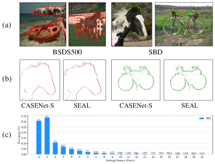
Figure 1. (a) Examples of noisy edge labels. Red for noisy labels, and green for clean. BSDS500 only provides noisy labels. (b) Illustration of the impact of label noise. CASENet-S produces more blurred edges than SEAL, especially on detailed structures. (c) Distribution of noisy-label shifts on SBD.

To arrive at it, we propose PNT-Edge towards robust edge detection with noisy labels through learning Pixel-level Noise Transitions. This transition function describes the label corruption process, i.e., noise transitions. And we achieve it by developing a novel Pixel-wise Shift Learning (PSL) module, which estimates the displacement field of noisy labels via a differentiable STN (Jaderberg et al., 2015) structure. Since clean labels are unavailable, it is hard to identify noise transitions merely through noisy labels (Han et al., 2020). A common solution is exploiting prior knowledge like “instances of similar appearance probably have similar transitions”  (Cheng et al., 2022) to help learn noise transition functions. Since labeling complex edge structures are much harder, such edges tend to contain more label noise as Fig. 3 shows. Considering this fact, we design a local edge density regularization to constrain the structure of the pixel-level noise transitions. Our aim is to encourage large shifts on latent clean edges with complicated local structures. Taking advantage of the designed PSL and the local edge density regularization, our PNT-Edge is able to fit the clean labels implicitly and thus yield thinner and more precise edge maps.

Experiments prove the effectiveness of PNT-Edge, which improves the ODS-F by 2.4% and mAP by 4.7% of the baseline on the re-annotated SBD test set with almost clean labels. We also surpass SEAL ODS-F by 1.3% and mAP by 1.6% on SBD. While Cityscapes contains low-level label noise, our method also achieves competitive ODS-F and better mAP compared with existing methods, i.e., 0.1% higher ODS-F and 4.3% higher mAP than SEAL. The proposed PNT-Edge can produce visually more precise edge maps than other methods. Our main contributions are summarized as follows:

• We propose a PNT-Edge model to train robust edge detectors with noisy labels by modeling the process of label corruption, i.e., pixel-level noise transition functions.

• We develop a novel PSL module to learn pixel-level noise transitions as a displacement field. And we design a local edge density regularization via prior knowledge to guide the estimation of noise transitions.

• Our PNT-Edge outperforms the SEAL by 1.3% ODS-F and 1.6% mAP on SBD. It also obtains competitive ODS-F and 4.3% higher mAP on Cityscapes than SEAL. Experiments on SBD and Cityscapes validate that our method can relieve the impact of label noise and produce more precise edges.

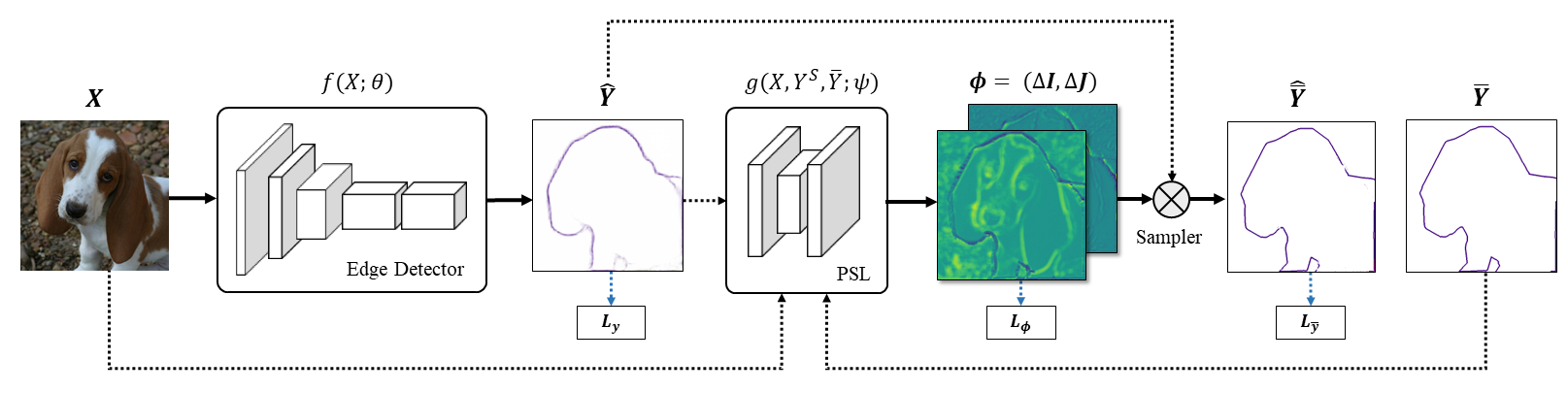
Figure 2. The architecture of PNT-Edge for edge detection with label noise. It contains an edge detector for edge detection and a PSL module for learning pixel-level noise transitions. We first train edge detector with noisy labels $\bar{Y}$. Then PSL learns $\phi$ for modeling label corruption and adapts prediction $\hat{Y}$ to $\hat{\bar{Y}}$. Through training edge detector with PSL, $\hat{Y}$ would finally approximate clean labels. Details refer to Sec. 3.2. Note that only the edge detector is required for producing the final edge maps.

2. Related Works

Learning with Noisy Labels

Since collecting clean labels for large datasets is expensive, label-noise learning is proposed to train robust models with label noise, especially for classification. Existing methods are generally divided into two categories: (1) Statistically-inconsistent methods employ heuristics like memorization effect (Arpit et al., 2017) to extract reliable examples (Jiang et al., 2018; Malach and Shalev-Shwartz, 2017), correct noisy labels (Yi and Wu, 2019) or design noise-robust loss functions (Patrini et al., 2017). (2) Statistically-consistent methods are proven to approximate the optimal classifiers trained on clean data (Patrini et al., 2017) if given enough data. But the key challenge for statistically-consistent methods is how to estimate noise transition matrices (Yao et al., 2020) accurately. Though estimating instance-independent transition matrices has been well-studied under assumptions like anchor points (Liu and Tao, 2015), real-life label noise is instance-dependent and more challenging to identify. Recent works like  (Cheng et al., 2022; Yao et al., 2021) incorporated prior knowledge and designed regularization to help identify instance-dependent noise transitions.

Segmentation with Noisy Labels

Semantic Segmentation also suffers from label noise, especially in semi-supervised learning and medical scenarios. Inspired by the success of label-noise learning in classification, researchers took similar heuristics such as proposing robust loss functions (Wang et al., 2020) or algorithms for noisy label detection and correction (Shu et al., 2019; Min et al., 2019). Specifically, such methods assumed adjacent pixels with similar features share the same label and captured local relationships by dense-CRF (Krähenbühl and Koltun, 2011), random walk (Bertasius et al., 2017), etc. For instance, Yi et al. (2021) proposed a graph-based framework to correct noisy labels. Recently, ADELE (Liu et al., 2022b) verified the memorization effect for segmentation and proposed a strategy to detect the memorization of each category for label correction.

Edge detection, commonly treated as a segmentation task, is vulnerable to noisy labels because of fine edge structures. Prior methods (Dollár and Zitnick, 2013) considered label noise during evaluation by setting a tolerance for matching edges. Later, to deal with multi-annotator bias, RDS (Liu and Lew, 2016) proposed to relax labels with Canny (1986), and RCF (Liu et al., 2017) designed an annotator-robust loss. Yang et al. (2016) refined noisy edges by dense-CRF as pre-processing but it was sensitive to background textures. SEAL (Yu et al., 2018) first employed a probabilistic model to align noisy labels via min-cost graph assignment and simultaneously trained the detector on refined labels. Similarly, STEAL (Acuna et al., 2019) utilized a level-set formulation to reason about real edges during training. From a different perspective from SEAL and STEAL, we handle noisy labels by estimating the transitions of noisy labels, so the edge detector can learn real edges implicitly. Thus, we can train robust edge detectors with noisy labels efficiently, without additional individual discrete optimization steps.

3. Methodology

3.1. Problem Setup

Following SEAL, this paper focuses on semantic edge detection with $C$ categories, which is commonly treated as a multi-label semantic segmentation task (Yu et al., 2017). Let $(X,Y)\in\mathcal{X}\times\mathcal{Y}$ denote an example drawing from the ideal dataset with clean labels, where the image $X=(x_{ij\cdot})\in R^{H\times W\times 3}$ and the ground-truth $Y=\{Y_{k}=(y_{ij}^{k})\in R^{H\times W}|k=1,2,\cdots,C\}$, $y_{ij}^{k}\in\{0,1\}$. Supposing the probabilities of different categories are independent following  (Yu et al., 2018; Acuna et al., 2019; Liu et al., 2022a), the goal of semantic edge detection formulates as:

(1) $$\max_{\theta}\ P(\hat{Y}|X;\theta)=\max_{\theta}\ \prod_{C}{P(\hat{Y_{k}}|X;\theta)},$$

where $\hat{Y}$ and $\hat{Y}_{k}$ denote the network predictions, and $\theta$ is the parameter of the semantic edge detector.

However, in real-life scenarios, we can only access a noisy observation $\bar{Y}$ of the ideal clean label $Y$. Therefore, if we train the network with $\bar{Y}$, the detector would eventually fit the noisy posterior. To separate the clean posterior $P(Y_{k}|X)$, we rewrite Eq. 1 as conditional probability as follows,

(2) $$\max_{\theta}\ P(\hat{\bar{Y}}|X;\theta)=\max_{\theta_{1},\theta_{2}}\ \prod_{C}{P(\hat{\bar{Y}}_{k}|\hat{Y}_{k},X;\theta_{1})}P(\hat{Y}_{k}|X;\theta_{2}),$$

where $\hat{\bar{Y}}$ and $\hat{\bar{Y}}_{k}$ denote the prediction of noisy labels, and $\theta_{1},\theta_{2}$ are model parameters. According to Eq. 2, if we can estimate the noise transition function $P(\hat{\bar{Y}}_{k}|\hat{Y}_{k},X)$, the clean posterior can be inferred from the noise transition and the noisy posterior. Thus, it is possible to train robust edge detectors implicitly by exploring noise transitions. For label-noise learning in classification, the noise transition matrix between different semantic categories has been widely discussed (Han et al., 2020). Here, for studying pixel-level label noise, we define a pixel-level transition function by the displacement field $\phi=(\Delta I,\Delta J)\in R^{H\times W\times 2}$ for learning pixel-wise shifts of noisy labels in edge detection, where $\Delta I=\{\Delta i\}_{H\times W},\Delta J=\{\Delta j\}_{H\times W}$ represent the pixel-wise shifts of noisy labels along the horizontal and vertical direction, respectively. Here $\phi$ is defined in Euler coordinates (Modersitzki, 2003). The relationship between clean and noisy labels formulates as:

(3) $$Y_{k}(i,\ j)=\bar{Y}_{k}(i+\Delta i,j+\Delta j).$$

Therefore, the key challenge is how to accurately estimate the displacement field $\phi$. Ideally, if both real and noisy labels are accessible, we can identify the displacement field $\phi$ by minimum-distance matching approximately. Because noisy edge labels would not move too far from real edge pixels. However, under the label-noise setting, clean edges are unknown. Fortunately, considering noisy labels only occupy a small part of the dataset, existing works have provided useful methods for extracting confident examples, i.e., probably clean examples, through heuristics like the memorization effect (Arpit et al., 2017). Therefore, we first check the memorization effect for edge detectors. Similar to ADELE (Liu et al., 2022b), we select the warm-up model with rapid increments of metrics on the training set and extract confident examples with high confidence (Jiang et al., 2018) (refer to Sec. 4.4). Then we can approximate the offsets from noisy labels to confident examples by minimum-distance matching. For the other latent clean edges, we can infer their offsets based on the continuity of edges and adjacent confident examples. Moreover, given the fact that complex edges are much harder to label correctly than those with simple structures, we design a local edge density regularization to encourage large shifts on latent clean edges with complicated local structures, which helps constrain the structure of noise transitions. The detailed instructions for the PNT-Edge model are as follows.

3.2. PNT-Edge

As shown in Fig. 2, our PNT-Edge model consists of two parts: 1) An edge detector $f(\cdot)$ for detecting edges or semantic edges; 2) A PSL module $g(\cdot)$ for estimating pixel-level noise transitions.

Edge Detector

While recent works (Zhen et al., 2020; Hu et al., 2019) have set new SOTA for semantic edge detection, we employ CASENet (Yu et al., 2017) as our semantic edge detector $f(X;\theta)$ following SEAL for fair comparison. The edge detection process is expressed as:

(4) $$\hat{Y}=f(X;\theta).$$

Note that CASENet can be replaced by other FCN-based edge detectors, and our PNT-Edge is edge-detector-agnostic.

Pixel-wise Shift Learning Module

To model label corruption according to Eq. 2, PSL module takes the image $X$, confident labels $\hat{Y}^{S}$, and noisy label $\bar{Y}$ to estimate the pixel-level transitions of noisy labels, where $\hat{Y}^{S}$ is computed by a confidence threshold $\tau$ as:

(5) $$\hat{Y}^{S}=\{\hat{y}^{s}_{ij}\ |\ p(\hat{y}_{ij})>\tau,s=1,2,\cdots,|S|\}.$$

The PSL module $g(X,\hat{Y}^{S},\bar{Y};\psi)$ comprises a localizer and a sampler, where $\psi$ denotes model parameters. The localizer is a 4-layer FCN with shortcuts and outputs displacement field $\phi$. Then the sampler transforms original prediction $\hat{Y}$ of edge detector to $\hat{\bar{Y}}$ according to the field $\phi$ by sampling as:

(6) $$\hat{\bar{Y}}=Sampler(\hat{Y},\phi),\ \phi=g(X,\hat{Y}^{S},\bar{Y};\psi).$$

Local Edge Density Regularization

Since the edge-label noise is class- and instance-dependent, it is hard to identify the noise transitions without prior knowledge. Generally, complicated edge structures are harder to label correctly because labeling such edges is more costly. This indicates such complex edges are prone to label noise. As a trade-off between label quality and efficiency, noisy labels are mostly over-smoothed. This is a common phenomenon among existing datasets. We verify this fact on SBD by calculating the density of real edges and the magnitude of corresponding shifts. In Fig. 3, large shifts tend to happen on edges with complicated local structures, i.e., high local edge density, and vice versa. Therefore, to help identify pixel-level noise transitions and guide pixel-wise shift estimation, we utilize this prior knowledge as a structural constraint on the displacement field $\phi$. The proposed local edge density regularization term is defined as:

(7) $$L_{dns}(D,C)=\frac{1}{HW}\sum_{i,j}{(d_{ij}-c_{ij})^{2}},$$

where local edge density $C=\{c_{ij}\}_{H\times W},\ c_{ij}=\frac{\sum{\mathbb{I}(y=1)}}{N\times N}$ is defined as the number of edge pixels at an $N\times N$ window centered at $(i,j)$. Since clean labels are unavailable, we estimate the local edge density with Canny (Canny, 1986). $D=\{d_{ij}\}_{H\times W},\ d_{ij}=\frac{\sqrt{(\Delta i)^{2}+(\Delta j)^{2}}}{d_{max}}$ is the normalized offsets measured by Euler distance, where $d_{max}$ is the maximum offset of each image. Notice that Eq. 7 does not strictly force $d_{ij}=c_{ij}$, but encourages learning large shifts on latent clean edges with complicated edge structure and vice versa.

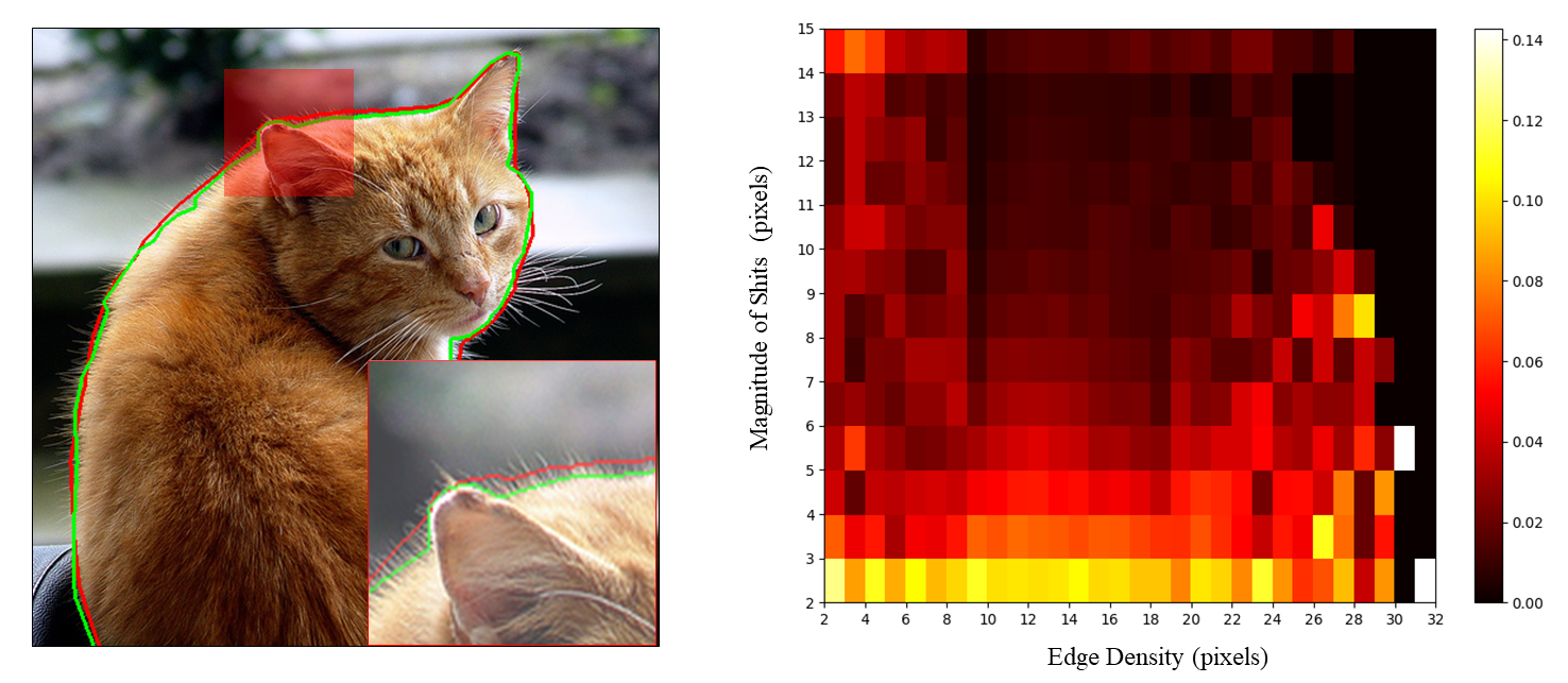
Figure 3. Clean and noisy labels, and distribution of noisy-label shifts and edge complexity measured by local edge density. Noisy labels show large offsets on complex structures.

Training Strategy

The whole training pipeline consists of three steps. First, we train the edge detector with noisy labels and select the warm-up model by observing learning curves similar to (Liu et al., 2022b). Second, we extract reliable examples with high confidence and train the PSL module to estimate the displacement field of noisy labels for modeling label corruption. Third, we append the PSL module to the edge detector for joint training. As expressed in Eq. 2, since PSL bridges the latent clean labels and noisy labels by the estimated pixel-level transitions, if the noise transitions are estimated accurately, the edge detector $f(X;\theta)$ would eventually fit clean labels. The training pipeline also refers to our Appendix.

To train the whole model effectively, carefully designed loss functions are essential. In general, we put constraints on the original edge prediction $\hat{Y}$, displacement field $\phi$ and transformed output $\hat{\bar{Y}}$, abbreviated as $L_{y}$, $L_{\phi}$ and $L_{\bar{y}}$ in Fig. 2. In detail, for warm-up training, since SEAL has validated that unweighted loss could bring thinner edge maps and better performance, we employ a multi-label loss without class-balance weight to train CASENet, commonly denoted as CASENet-S, which is computed as:

(8) $$L_{edge}(\hat{Y},\bar{Y})=\sum_{k}\sum_{i,j}-\bar{y}^{k}_{ij}log(\hat{y}^{k}_{ij})-(1-\bar{y}^{k}_{ij})log(1-\hat{y}^{k}_{ij}).$$

For training the PSL module, we employ three kinds of losses. First, we directly employ the mean squared error to supervise the shifts on confident examples as follows,

(9) $$L_{sup}(\phi_{S},\phi^{*}_{S})=\frac{1}{|S|}\sum_{S}{(\phi(y^{s})-\phi^{*}(y^{s}))^{2}},$$

where the ground-truth shifts $\phi^{*}_{S}$ are produced by minimum-distance matching between confident labels and noisy labels. Second, since the ideal displacement field would produce $\bar{Y}$ after transformation, we employ a similarity constraint on $\hat{\bar{Y}}$. We empirically find that MSE loss works better than CE in predicting the displacement field, and the similarity loss is formulated as:

(10) $$L_{sim}(\hat{\bar{Y}},\bar{Y})=\frac{1}{HW}\sum_{i,j}{(\hat{\bar{y}}_{ij}-\bar{y}_{ij})^{2}}.$$

Third, given both clean and noisy edge labels are continuous, the displacement field should be smooth as well. This property helps to infer pixel-wise shifts of edges around confident ones. So, we regularize the field with an L2-loss to encourage smoothness as,

(11) $$L_{smth}(\phi)=||\nabla(\Delta I)||^{2}+||\nabla(\Delta J)||^{2}.$$

To help identify the noise transition function, our local edge density regularization is added and implemented as Eq. 7. When conducting experiments, we find the proposed $L_{dns}$ also regularizes the smoothness of the displacement field. Details refer to Sec. 4.6. Therefore, the overall loss for PSL training is formulated as follows, where $\{\alpha_{i}\}_{i=1}^{4}$ are loss weights.

(12) $$L_{PSL}=\alpha_{1}L_{sup}+\alpha_{2}L_{sim}+\alpha_{3}L_{smth}+\alpha_{4}L_{dns}.$$

For the joint training of edge detector and PSL, we first intuitively supervise the final output $\hat{\bar{Y}}$ by the noisy label $\bar{Y}$ as follows,

(13) $$L_{edge}(\hat{\bar{Y}},\bar{Y})=\sum_{k}\sum_{i,j}-\bar{y}^{k}_{ij}log(\hat{\bar{y}}^{k}_{ij})-(1-\bar{y}^{k}_{ij})log(1-\hat{\bar{y}}^{k}_{ij}).$$

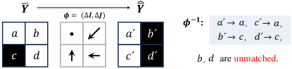
Figure 4. Illustration of unmatched pixels and $\phi^{-1}$ in Eq.14.

Additionally, we force the predictions of unmatched pixels to be zero. Because $\phi$ is defined as a many-to-one mapping, there exist unmatched pixels in the output $\hat{Y}$ as illustrated in Fig.4. If only the final output $\hat{\bar{Y}}$ is supervised, the predictions of such unmatched pixels will be uncontrolled, which is undesirable. Experimental evidence refers to Sec. 4.6. The unmatched loss is computed as:

(14) $$L_{um}=\sum_{k}\sum_{(i,j)\notin\phi^{-1}}-log(1-\hat{y}^{k}_{ij}),$$

where $\phi^{-1}$ denotes the generalized inverse of $\phi$. Thus, the overall loss for joint training is as follows:

(15) $$L_{joint}=\beta_{1}L_{edge}+\beta_{2}L_{um},$$

where $\{\beta_{i}\}_{i=1}^{2}$ are weights. Since both losses are equally important, we empirically set $\beta_{1}=\beta_{2}=1$ for simplicity.

3.3. Discussion

In this part, we further analyze our work by making comparisons with some previous related works.

First, our method differs from label-noise learning for classification (Han et al., 2020), where statistically-consistent methods (Patrini et al., 2017) proposes to estimate the noise transitions between categories. In comparison, aiming at edge detection with label noise, this paper explores noise transition functions at pixel level through the displacement field. We also incorporate prior knowledge of edge-label noise and design a regularization term for learning noise transitions better.

Second, it is worth noting that our method varies from current works on addressing label noise in segmentation. These methods attempt to alleviate the issue through early stopping (Liu et al., 2022b), prediction consistency (Min et al., 2019), modeling local affinity by GAT (Yi et al., 2021), low-level cues (Shu et al., 2019), etc. Such methods rely on the affinity between boundary and interior pixels for label correction, but it is unavailable in edge detection. Moreover, noise transition is rarely explored in segmentation. This paper aims to implicitly learn clean labels by modeling noisy label corruption, rather than label refinements.

Third, learning pixel offsets is often exploited to refine predictions. For example, SharpContour (Zhu et al., 2022) proposed a contour-based model to improve boundary quality for instance segmentation as post-processing. Recent E2EC (Zhang et al., 2022) proposed a global contour deformation module and a multi-direction alignment scheme to optimize boundaries for contour-based instance segmentation. DELSE (Wang et al., 2019) predicted pixel motions and deformed the contour by curve evolution for interactive object segmentation. Different from these efforts, we attempt to implicitly learn robust edge detectors by employing pixel offsets as transitions between clean and noisy labels.

4. Experiments

4.1. Datasets

Semantic Boundary Dataset (SBD)

It contains 11,355 images from the PASCAL VOC 2011 trainval set with category- and instance-level semantic edges of 20 classes. There are 8,498 images for training and 2,857 images for testing. SEAL provided a re-annotated sub-test set of 1,059 images with almost clean labels for evaluation. We randomly sample 1,000 images from the training set and 50% of the sub-test set for validation. Here we only focus on instance-sensitive edges following SEAL and STEAL.

Cityscapes

It contains 2,975 road images for training, 500 for validation, and 1,525 for testing. SEAL provided edge labels. We test on the validation set following SEAL. Since Cityscapes is annotated by experts, it contains much less label noise than SBD. Considering that Cityscapes does not provide clean labels, we evaluate performance on noisy labels with relaxed criteria following SEAL.

4.2. Evaluation Metrics

We employ the same metrics as SEAL and test on clean labels. We report maximum F-measure at optimal dataset scale (ODS-F) and mAP, and set the matching tolerance to 0.0075 ($\approx$4 pixels) for SBD and 0.0035 ($\approx$8 pixels) for Cityscapes. Following SEAL, we employ two settings: 1) “Thin” for matching the thinned prediction with ground truth, and 2) “Raw” for matching the raw prediction with ground truth. Our method does not employ NMS post-processing.

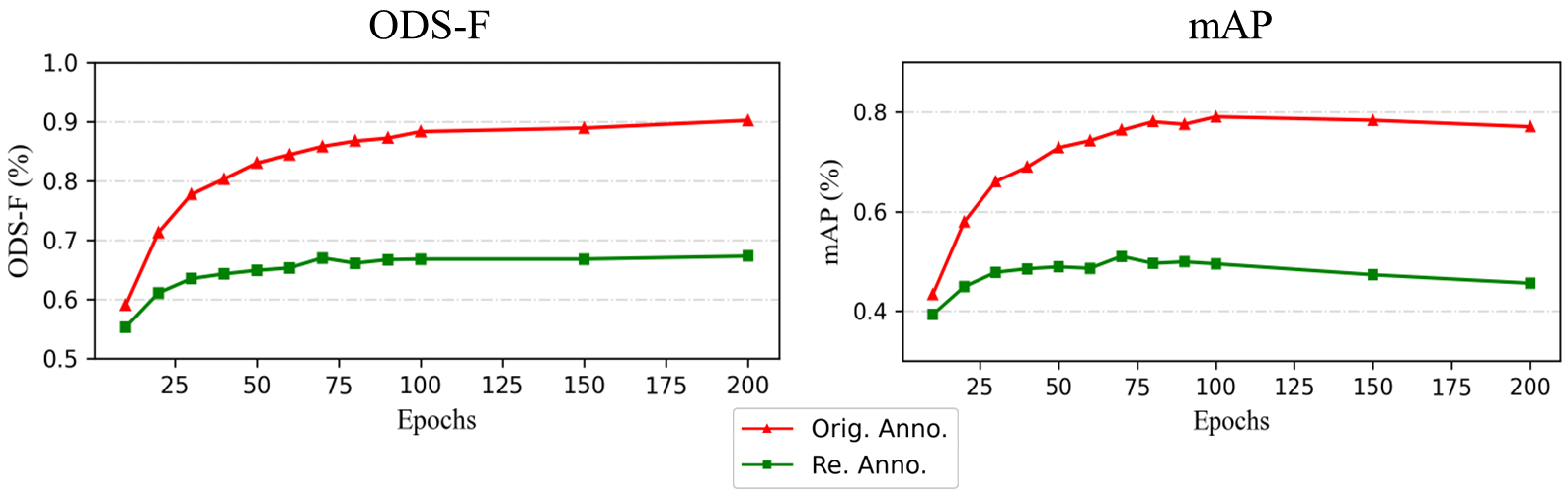
Figure 5. Evaluation protocols on the sub-test of SBD that validate the memorization effect in edge detection.

Setting	Metric	Method	aero	bike	bird	boat	bottle	bus	car	cat	chair	cow	table	dog	horse	mbike	person	plant	sheep	sofa	train	tv	AVG.
Thin	ODS-F	CASENet	0.743	0.597	0.732	0.478	0.668	0.787	0.673	0.760	0.475	0.696	0.361	0.756	0.726	0.613	0.746	0.425	0.715	0.487	0.716	0.552	0.635
		CASENet-S	0.759	0.663	0.755	0.519	0.664	0.798	0.710	0.788	0.501	0.698	0.397	0.772	0.746	0.649	0.769	0.471	0.727	0.515	0.727	0.573	0.658
		SEAL	0.781	0.659	0.767	0.524	0.684	0.800	0.706	0.796	0.500	0.726	0.414	0.782	0.750	0.655	0.784	0.492	0.730	0.522	0.739	0.582	0.669
		STEAL†	0.790	0.658	0.773	0.546	0.686	0.815	0.711	0.784	0.523	0.737	0.428	0.792	0.764	0.668	0.782	0.491	0.752	0.500	0.749	0.594	0.677
		Ours	0.787	0.680	0.770	0.547	0.697	0.813	0.714	0.786	0.503	0.750	0.436	0.779	0.757	0.666	0.784	0.518	0.784	0.516	0.748	0.608	0.682
	mAP	CASENet	0.537	0.444	0.479	0.309	0.489	0.596	0.523	0.629	0.360	0.494	0.253	0.591	0.498	0.423	0.599	0.272	0.531	0.409	0.490	0.374	0.465
		CASENet-S	0.677	0.519	0.690	0.406	0.627	0.735	0.636	0.753	0.409	0.606	0.304	0.722	0.654	0.558	0.730	0.332	0.630	0.449	0.671	0.484	0.580
		SEAL	0.733	0.568	0.720	0.426	0.661	0.754	0.661	0.781	0.420	0.659	0.334	0.757	0.689	0.575	0.764	0.376	0.675	0.468	0.692	0.513	0.611
		STEAL†	0.747	0.595	0.742	0.436	0.658	0.775	0.677	0.774	0.428	0.707	0.315	0.775	0.750	0.607	0.773	0.381	0.701	0.389	0.714	0.503	0.622
		Ours	0.750	0.619	0.728	0.440	0.673	0.761	0.665	0.771	0.412	0.699	0.334	0.753	0.725	0.606	0.781	0.429	0.714	0.434	0.699	0.541	0.627
Raw	ODS-F	CASENet	0.657	0.514	0.649	0.429	0.572	0.682	0.582	0.659	0.453	0.597	0.329	0.640	0.657	0.524	0.654	0.408	0.650	0.428	0.613	0.477	0.559
		CASENet-S	0.689	0.557	0.709	0.473	0.619	0.715	0.647	0.712	0.480	0.648	0.372	0.691	0.688	0.581	0.702	0.442	0.687	0.461	0.657	0.525	0.603
		SEAL	0.753	0.605	0.752	0.512	0.654	0.761	0.679	0.760	0.497	0.694	0.399	0.747	0.728	0.621	0.741	0.482	0.723	0.492	0.705	0.566	0.644
		STEAL†	0.709	0.559	0.716	0.476	0.616	0.726	0.646	0.702	0.475	0.674	0.373	0.706	0.694	0.591	0.692	0.443	0.691	0.426	0.677	0.535	0.606
		Ours	0.766	0.660	0.767	0.543	0.673	0.776	0.696	0.766	0.505	0.734	0.423	0.758	0.751	0.644	0.771	0.517	0.781	0.493	0.717	0.598	0.667
	mAP	CASENet	0.668	0.509	0.596	0.346	0.510	0.675	0.563	0.680	0.416	0.547	0.263	0.657	0.668	0.480	0.701	0.348	0.618	0.390	0.615	0.423	0.534
		CASENet-S	0.755	0.575	0.750	0.455	0.625	0.755	0.662	0.762	0.456	0.657	0.309	0.738	0.730	0.598	0.763	0.391	0.701	0.420	0.700	0.504	0.615
		SEAL	0.810	0.634	0.792	0.496	0.668	0.794	0.699	0.810	0.472	0.705	0.344	0.797	0.766	0.633	0.803	0.449	0.736	0.452	0.739	0.539	0.657
		STEAL†	0.756	0.559	0.749	0.432	0.619	0.751	0.653	0.746	0.419	0.677	0.287	0.744	0.736	0.592	0.740	0.382	0.695	0.354	0.710	0.493	0.605
		Ours	0.790	0.662	0.774	0.492	0.664	0.784	0.688	0.797	0.434	0.727	0.335	0.775	0.762	0.634	0.801	0.477	0.769	0.414	0.736	0.555	0.653

Table 1. Comparisons with previous SOTA methods on the re-annotated SBD test set. “AVG.” and ^† denote category-averaged performance and using NMS for post-processing, respectively.

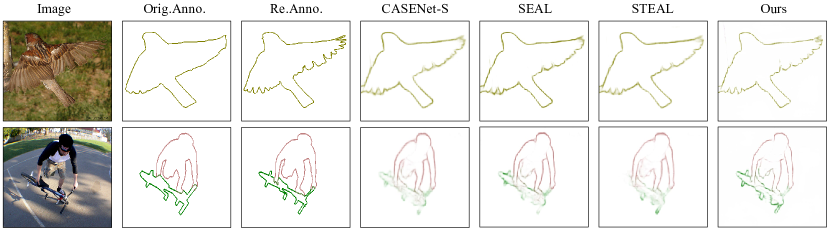
Figure 6. Example results on SBD. Our method generates more precise edge maps with clear details.

4.3. Implementation Details

Following SEAL, we crop images by $472\times 472$ for training and employ scaling and random flipping. We initialize CASENet with pre-trained parameters provided by SEAL and randomly initialize PSL module. For warm-up training, we employ a learning rate 5e-8$/$2.5e-8 and train $30$ epochs for SBD$/$Cityscapes with batch size 8 and learning rate decay. For training PSL, we set the learning rate as 1e-6 and freeze CASENet. We train PSL module for 10 epochs and decay the learning rate by $0.1$ every $10k$. For joint training, we initialize CASENet with warm-up parameters and freeze PSL module. Then we change the learning rate to 1e-9 and train for another 10 epochs while keeping other settings the same. For hyper-parameters, we empirically set $\tau=0.1,\alpha_{1}=0.01,\alpha_{2}=1,\alpha_{3}=0,\alpha_{4}=3$ according to Sec. 4.6. All experiments are conducted on NVIDIA GeForce RTX 3090 using PyTorch.

4.4. Memorization Effect in Edge Detection

We first revisit memorization effect in edge detection. Since clean training samples are required for evaluation, we divide the re-annotated SBD test set into 847$/$212 images for train/test and train CASENet-S with noisy labels. Fig. 5 reports the performance on noisy and clean labels. While metrics on noisy labels keep increasing, metrics on clean labels only increase at early stages. It verifies detectors first fit clean labels and then memorize noisy labels.

Moreover, we notice a rapid increment of ODS-F and mAP on noisy labels at about 20 epochs when metrics on clean labels are saturated. According to ADELE (2022b), we select the warm-up model with the rapid increment of metrics on the training set. We further check the performance of models at around 20 epochs and find they perform well on clean labels, which validates the rationality of this strategy. For Cityscapes without clean labels, we employ the same setting and select models around 20 epochs as our warm-up model which also performs well on the test set.

Setting	Metric	Method	road	sidewalk	building	wall	fence	pole	t-light	t-sign	veg	terrain	sky	person	rider	car	truck	bus	train	motor	bike	AVG.
Thin	ODS-F	CASENet	0.862	0.748	0.748	0.482	0.468	0.729	0.703	0.735	0.794	0.567	0.865	0.806	0.666	0.883	0.495	0.672	0.498	0.566	0.718	0.684
		CASENet-S	0.876	0.771	0.762	0.492	0.467	0.755	0.715	0.753	0.806	0.597	0.867	0.817	0.683	0.893	0.513	0.688	0.442	0.552	0.726	0.693
		SEAL	0.878	0.777	0.763	0.481	0.468	0.756	0.713	0.754	0.810	0.602	0.873	0.819	0.690	0.891	0.508	0.690	0.450	0.540	0.727	0.695
		STEAL†	0.879	0.777	0.773	0.494	0.491	0.790	0.746	0.764	0.821	0.597	0.881	0.808	0.701	0.836	0.519	0.675	0.531	0.557	0.742	0.704
		Ours	0.878	0.775	0.766	0.494	0.473	0.787	0.734	0.756	0.810	0.591	0.866	0.820	0.705	0.887	0.482	0.680	0.433	0.552	0.741	0.696
	mAP	CASENet	0.542	0.640	0.661	0.393	0.372	0.580	0.606	0.680	0.693	0.477	0.737	0.697	0.583	0.672	0.406	0.550	0.387	0.492	0.603	0.567
		CASENet-S	0.894	0.757	0.736	0.438	0.390	0.665	0.672	0.745	0.774	0.541	0.822	0.785	0.619	0.884	0.449	0.688	0.360	0.485	0.675	0.651
		SEAL	0.772	0.762	0.759	0.433	0.401	0.657	0.684	0.762	0.788	0.565	0.824	0.809	0.639	0.859	0.459	0.688	0.384	0.488	0.705	0.655
		STEAL†	0.907	0.800	0.801	0.409	0.413	0.800	0.755	0.778	0.848	0.569	0.900	0.835	0.687	0.831	0.436	0.660	0.457	0.511	0.757	0.692
		Ours	0.905	0.800	0.796	0.432	0.419	0.794	0.749	0.782	0.842	0.578	0.880	0.859	0.705	0.920	0.445	0.690	0.373	0.525	0.774	0.698
Raw	ODS-F	CASENet	0.641	0.585	0.664	0.311	0.325	0.712	0.621	0.645	0.708	0.438	0.782	0.722	0.565	0.753	0.328	0.471	0.281	0.431	0.609	0.558
		CASENet-S	0.774	0.692	0.704	0.358	0.351	0.740	0.654	0.680	0.747	0.512	0.804	0.759	0.596	0.829	0.358	0.528	0.293	0.424	0.643	0.602
		SEAL	0.822	0.717	0.728	0.356	0.353	0.762	0.665	0.694	0.773	0.538	0.830	0.777	0.620	0.850	0.367	0.544	0.308	0.424	0.662	0.620
		STEAL†	0.758	0.685	0.699	0.349	0.361	0.734	0.668	0.677	0.735	0.497	0.787	0.729	0.591	0.765	0.353	0.528	0.377	0.438	0.638	0.598
		Ours	0.807	0.730	0.763	0.367	0.373	0.785	0.701	0.727	0.804	0.524	0.837	0.805	0.657	0.866	0.347	0.542	0.288	0.449	0.714	0.636
	mAP	CASENet	0.479	0.568	0.684	0.228	0.236	0.741	0.624	0.653	0.744	0.380	0.797	0.766	0.565	0.721	0.215	0.364	0.202	0.382	0.647	0.526
		CASENet-S	0.819	0.732	0.755	0.287	0.254	0.798	0.686	0.716	0.810	0.489	0.813	0.816	0.598	0.893	0.255	0.499	0.185	0.367	0.698	0.604
		SEAL	0.780	0.740	0.777	0.277	0.256	0.796	0.686	0.732	0.834	0.508	0.825	0.828	0.621	0.888	0.257	0.507	0.195	0.356	0.717	0.609
		STEAL†	0.811	0.728	0.750	0.263	0.263	0.791	0.693	0.719	0.799	0.472	0.804	0.788	0.581	0.811	0.244	0.490	0.278	0.377	0.683	0.597
		Ours	0.818	0.745	0.793	0.258	0.271	0.817	0.708	0.752	0.846	0.477	0.830	0.837	0.645	0.911	0.254	0.492	0.187	0.373	0.755	0.619

Table 2. Comparisons with previous SOTA methods on Cityscapes. “AVG.” and ^† denote category-averaged performance and using NMS for post-processing, respectively.

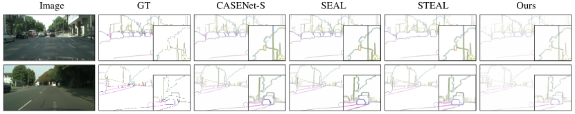
Figure 7. Example results on Cityscapes. Our method obtains much thinner and more accurate edge maps than other methods.

4.5. Comparison with previous SOTA Methods

We compare our method with CASENet, SEAL, and STEAL on SBD and Cityscapes. The baseline is CASENet-S, i.e., CASENet with the class-unweighted loss. Note that SEAL, STEAL, and our method are all built on CASENet-S with the ResNet-101 backbone. Our PNT-Edge model does not employ NMS for post-processing, as we only observe very slight improvements in our experiments. More discussions about the impact of NMS can be found in our Appendix.

Performance on SBD

The performance on re-annotated test set is reported in Tab. 1. Our method achieves the highest ODS-F under both settings, surpassing the baseline by 2.4% and 4.7%. It also outperforms SEAL ODS-F by 1.3% and mAP by 1.6% under “Thin” setting. Under “Raw” setting, our method obtains 2.3% higher ODS-F but lower mAP than SEAL (0.653 v.s. 0.657). Since SEAL generates thicker edges than ours as shown in Fig. 6, it causes better recall but worse precision. Moreover, our method obtains competitive results with STEAL which employs NMS for post-processing. Qualitative results in Fig. 6 further validate the effectiveness of our method. Fig. 8 visualizes predicted noise transitions, i.e., displacement fields.

Performance on Cityscapes

Following SEAL, we test on original labels that contain low-level label noise. The results are listed in Tab. 2. Under “Thin” setting, our method obtains competitive performance on ODS-F compared with the baseline and previous SOTA approaches because of little label noise on the Cityscapes. But we notice that PNT-Edge surpasses the baseline mAP enormously by 4.7%. This is because our method can fit ground truth better with few blurs as visualized in Fig. 7. Moreover, our method achieves the best performance on both ODS-F and mAP under “Raw” setting, which proves PNT-Edge can produce precise edge maps even without post-processing. Our method performs best under even stricter criteria as delivered in Sec. 4.7.

4.6. Ablation Study

We validate the impact of hyper-parameters and training strategies on SBD. We conduct experiments on the original validation set (Val-noisy) with noisy labels and a 50% random sampled re-annotated test set (Val-clean) with clean labels. The baseline is CASENet-S.

Impact of confident threshold $\tau$ and loss weight $\alpha_{4}$ for $L_{dns}$

To analyze the effect of confident-sample extraction and local edge density regularization, we experiment with different settings of $\tau$ and $\alpha_{4}$ and report in Tab. 3. For one thing, a lower $\tau$ leads to higher ODS-F on both noisy and clean labels, but a too-low $\tau$ degrades mAP remarkably, especially on clean labels. The reasons are two folds. First, the confidence of predicted edge maps is relatively low because of unweighted loss functions. Second, more confident examples help learn better noise transitions, but too low $\tau$ would introduce noisy examples and degrade performance. For another, when $\alpha_{4}$ increases, ODS-F increases consistently. However, mAP improves first and then decreases on Val-noisy and Val-clean. To make a trade-off between ODS-F and mAP on the clean labels, we choose $\tau=0.1,\alpha_{4}=3$ for experiments, where our method outperforms the baseline ODS-F by 1.3% and mAP by 4.4%. This fact verifies the effectiveness of our method. Note that though better performance on noisy labels indicates probably better performance on clean labels, it is not always the fact. It is possible to take metrics on noisy labels for reference only when clean labels are unavailable and the label noise is at a low level.

$\tau$	$\alpha_{4}$	Val-noisy		Val-clean
		ODS-F	mAP	ODS-F	mAP
Baseline		0.722	0.710	0.653	0.579
$0.01$	$0.0$	0.736	0.719	0.672	0.590
	$1.0$	0.729	0.721	0.669	0.613
	$2.0$	0.729	0.721	0.669	0.612
	$3.0$	0.729	0.720	0.666	0.607
	$5.0$	0.729	0.717	0.659	0.586
$0.1$	$0.0$	0.717	0.706	0.652	0.605
	$1.0$	0.718	0.709	0.651	0.607
	$2.0$	0.723	0.717	0.662	0.626
	$3.0$	0.727	0.723	0.666	0.623
	$5.0$	0.727	0.721	0.669	0.621
$0.2$	$0.0$	0.691	0.677	0.617	0.560

Table 3. Discussions of confident threshold $\tau$ and loss weight $\alpha_{4}$ for $L_{dns}$. Red indicates the trade-off setting.

Strategy	Val-noisy		Val-clean
	ODS-F	mAP	ODS-F	mAP
Label Correction	0.678	0.653	0.610	0.537
Joint Training	0.717	0.706	0.652	0.605

Table 4. Comparison of different training strategies on SBD.

Joint Training v.s. Label Correction

To further validate the effectiveness of our method, we compare two kinds of training strategies: joint training and label correction. The joint training is delineated in Sec. 3.2. For label correction, we employ $\phi^{-1}$ to refine noisy labels and then train CASENet-S with refined labels. Referring to Tab. 4, joint training is proved to be more effective than label correction. Because PSL module would dynamically adapt noisy labels through joint training. Besides, generating refined labels for the whole dataset is time-consuming. As a result, we employ the joint training strategy in PNT-Edge.

Effect of loss functions

As Tab. 5 shows, all loss functions help improve the performance on Val-clean and Val-noisy, but smooth loss $L_{smth}$ shows useless. Because the local edge density regularization, which encourages similar displacements on pixels with similar local edge densities, also works for smooth regularization. Tab. 5 also verifies the effectiveness of the proposed local edge density regularization term in pixel-level noise-transition identification. Moreover, the unmatched loss plays an important role in producing precise edge maps with high mAP.

PSL				Joint		Val-noisy		Val-clean
$L_{sup}$	$L_{sim}$	$L_{smth}$	$L_{dns}$	$L_{edge}$	$L_{um}$	ODS-F	mAP	ODS-F	mAP
$\checkmark$				$\checkmark$	$\checkmark$	0.679	0.659	0.603	0.538
$\checkmark$		$\checkmark$	$\checkmark$	$\checkmark$	$\checkmark$	0.716	0.703	0.642	0.586
$\checkmark$	$\checkmark$		$\checkmark$	$\checkmark$	$\checkmark$	0.726	0.720	0.668	0.627
$\checkmark$	$\checkmark$	$\checkmark$		$\checkmark$	$\checkmark$	0.717	0.706	0.652	0.605
$\checkmark$	$\checkmark$	$\checkmark$	$\checkmark$	$\checkmark$		0.723	0.461	0.659	0.369
$\checkmark$	$\checkmark$	$\checkmark$	$\checkmark$	$\checkmark$	$\checkmark$	0.727	0.723	0.666	0.623

Table 5. Effects of loss functions. We are more concerned about the results on Val-clean since our goal is to predict clean edges. Red indicates our experiment setting.

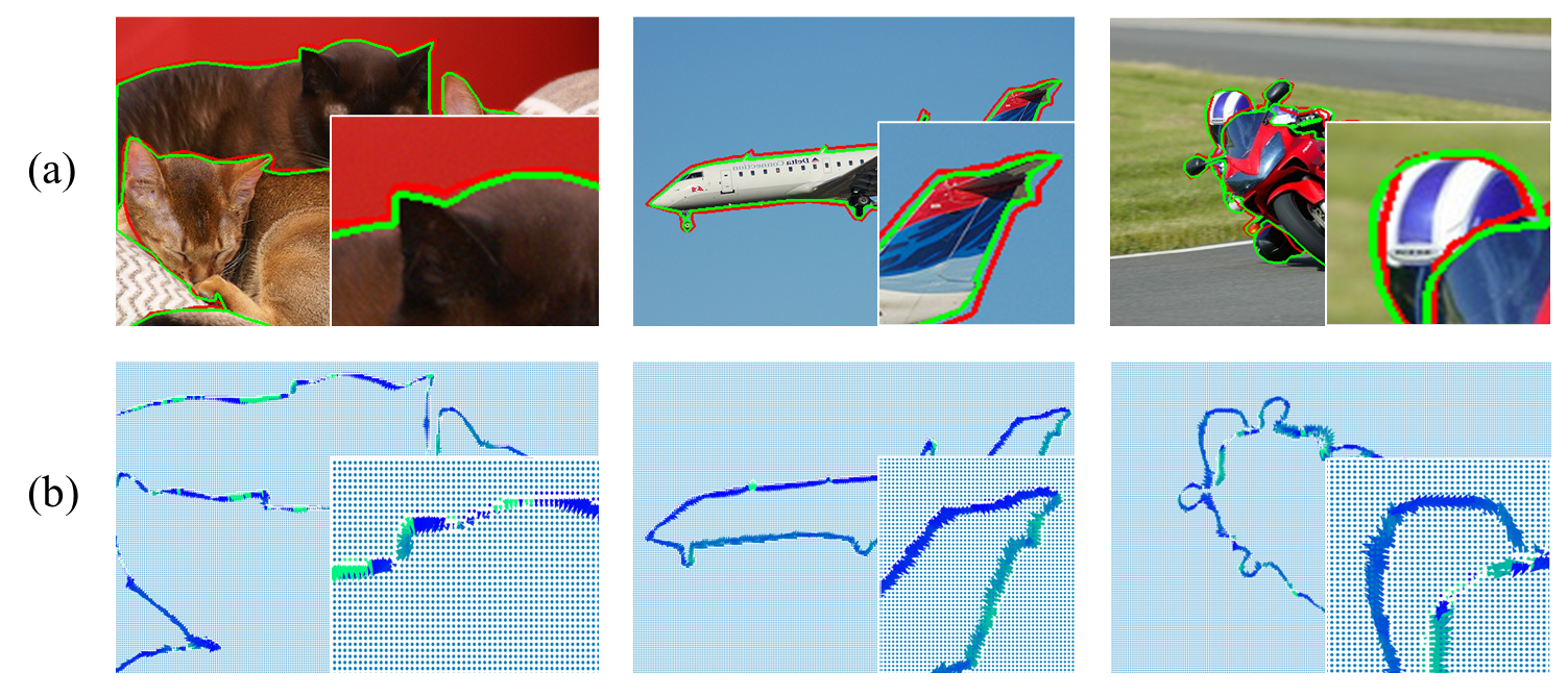
Figure 8. (a) SBD examples with both clean(green) and noisy labels(red). (b) Visualized pixel-level noise transitions.

4.7. Discussions

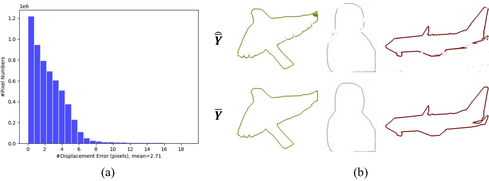
Figure 9. Error analysis. (a) Error histogram between predicted transitions with min-distance-matching results. (b) Comparison of transformed prediction $\hat{\bar{Y}}$ and noisy label $\bar{Y}$.

Noise-transition error analysis

To analyze the error of the predicted noise transition, i.e., displacement field $\phi$, we first compare with the min-distance-matching result on SBD. The error histogram in Fig. 9(a) reports an average error of 2.71 pixels. It is reasonable because of the gaps between min-distance-matching results and the ideal ground-truth transitions. Furthermore, considering that ideal transitions will produce high-quality predictions of the noisy label $\bar{Y}$, we compare the transformed edge prediction $\hat{\bar{Y}}$ with noisy label $\bar{Y}$. The ODS-F of $\hat{\bar{Y}}$ achieve 0.790 under “RAW” setting, indicating the predicted transition $\phi$ models label corruption well as shown in Fig. 9(b). Visualized displacement fields refer to Fig. 8.

5. Conclusion

This paper proposes PNT-Edge to tackle label noise for edge detection via modeling label corruption. To achieve it, we develop a PSL module to learn pixel-level noise transitions. And a local edge density regularization is proposed to help estimate such transitions via prior knowledge. Our method outperforms SEAL ODS-F by 1.3% and mAP by 1.6% on SBD and obtains competitive ODS-F and 4.3% higher mAP than SEAL on Cityscapes. The proposed PNT-Edge proves to be effective in relieving the impact of label noise and producing more precise edge maps.

Appendix A Appendix

A.1. The Overall Pipeline of PNT-Edge

We summarize the overall training pipeline of our PNT-Edge in Alg.1. It consists of three steps: a) warm-up training of the edge detector with noisy labels, b) training the PSL module with reliable examples to model the label corruption of noisy labels, and c) joint training of the edge detector and PSL with noisy labels.

A.2. More Discussions

Discussion of NMS Post-processing

To validate that PNT-Edge can generate crisp edge predictions without NMS, we further conduct experiments with NMS and report the results in Tab.6. While STEAL employed NMS, our method outperforms STEAL by 0.5% ODS-F and 0.5% mAP on SBD under the ‘Thin’ setting without NMS. Moreover, we find NMS brings limited increments to our method, which indicates our method directly generates crisp edge predictions without NMS post-processing. On the other hand, since NMS helps to relieve the blurred edge predictions caused by label noise, the results further validate the effectiveness of our method in relieving the impact of label noise.

Method	ODS-F	mAP
STEAL (NMS)	0.677	0.622
Ours (w/o NMS)	0.682	0.627
Ours (NMS)	0.685	0.627

Table 6. Model size and computational complexity for training. PNT-Edge does not bring additional cost for inference.

Performance under stricter criteria

To illustrate advances of our method, Tab. 7 compares the performance under stricter criteria i.e., lower matching threshold as 0.00175($\approx$ 4 pixels) and 0.000875($\approx$ 2 pixels) with previous approaches on Cityscapes. Our PNT-Edge achieves SOTA on both settings, surpassing the baseline ODS-F by 6.9% and mAP by 7.5% impressively under a 0.00175 threshold. Under an even stricter threshold of 0.000875, our method also obtains the best performance. These results prove our method produces crisp and precise edge maps effectively.

Model size and computational complexity

Since PSL is only an auxiliary module for tackling label noise via modeling label corruption during the training process, our method does not bring additional computation for inference. Tab. 8 compares the model size and computational complexity with the baseline CASENet-S for model training. Our PNT-Edge provides an effective training strategy to tackle noisy edge labels at the cost of negligible 0.16M more parameters and 15.4% FLOPs additional computation.

Threshold	Method	ODS-F(%)	mAP(%)
0.00175	CASENet	0.420	0.343
	CASENet-S	0.457	0.436
	SEAL	0.487	0.466
	STEAL†	0.444	0.413
	Ours	0.526	0.521
0.000875	CASENet	0.372	0.285
	CASENet-S	0.404	0.359
	SEAL	0.427	0.380
	STEAL†	0.396	0.347
	Ours	0.453	0.418

Table 7. Performance comparison under stricter criteria on Cityscapes. Our method achieves the best performance under stricter criteria, i.e., lower matching threshold.

Method	Params(M)	FLOPs(G)
CASENet-S	42.44	175.6
Ours	42.60	202.6

Table 8. Model size and computational complexity for training. PNT-Edge does not bring additional cost for inference.

Algorithm 1 PNT-Edge for noisy edge labels learning

Input: Noisy training set $\bar{D}=\{X_{i},\bar{Y_{i}}\}_{i=1}^{N}$, threshold $\tau$.                      
Output: Noise-robust edge detector $f(X;\hat{\theta})$.

1:  $//$ Step 1: Warm-up training

2:  Train the edge detector on the noisy dataset $\bar{D}$ to obtain the initial detector $f(X;\theta_{0})$ with Eq.8.

3:  $//$ Step 2: Train the PSL module

4:  for $i=1$ to $N$ do

5:     Extract confident labels $Y^{S}_{i}$ as Eq.5 with $f(X;\theta_{0})$;

6:     Generate field $\phi$ and transformed output $\hat{\bar{Y}}$ as Eq.6;

7:     Compute the loss as Eq.12;

8:     Optimize the parameter $\psi$ by SGD;

9:  end for

10:  return $\hat{\psi}$

11:  $//$ Step 3: Train the edge detector with PSL

12:  for $n=1$ to $N$ do

13:     Generate predictions $\hat{Y}_{i},\hat{\bar{Y}}_{i}$ by $f\circ g$ as Eq.4 and Eq.6;

14:     Compute the loss as Eq.15;

15:     Optimize the parameter $\theta$ by SGD;

16:  end for

17:  return $\hat{\theta}$

Appendix B General Edge Detection

B.1. Apply PNT-Edge to General Edge Detection

In our paper, we mainly focus on semantic edges for a fair comparison with previous works on noisy edges, i.e., SEAL and STEAL. Since our method is edge-detector-agnostic, it is also easy to apply our method to general edge detection. Here is an instruction.

1. Replace the semantic edge detector (i.e., CASENet) with the general edge detector (i.e., HED and RCF).

2. Use the general edge detection loss function, i.e., binary cross-entropy loss, instead of the multi-classification loss. And no more changes are needed.

3. Follow the same training procedure as Alg.1, and implement warm-up training, PSL-module training, and joint-training of the edge detector with PSL step by step.

Method	Thin			Raw
	ODS-F	OIS-F	mAP	ODS-F	OIS-F	mAP
HED	0.756	0.774	0.665	0.600	0.619	0.601
HED-PNT	0.767 $\uparrow 0.011$	0.786 $\uparrow 0.012$	0.734 $\uparrow 0.069$	0.654 $\uparrow 0.054$	0.665 $\uparrow 0.046$	0.698 $\uparrow 0.097$
RCF	0.765	0.781	0.676	0.627	0.642	0.637
RCF-PNT	0.771 $\uparrow 0.006$	0.787 $\uparrow 0.007$	0.723 $\uparrow 0.047$	0.642 $\uparrow 0.015$	0.651 $\uparrow 0.009$	0.684 $\uparrow 0.047$

Table 9. Performance comparison of our method, i.e., HED-PNT and RCF-PNT, with their baseline models on BSDS500. Our method brings consistent improvements to the baseline under all settings for the general-edge detection task.

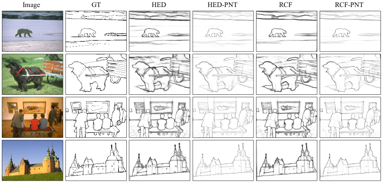
Figure 10. Example results of our PNT-Edge model and the baseline on BSDS500. Our method can produce more precise edge maps for general edge detection by relieving the label noise issue.

B.2. Results on BSDS500

We conduct experiments on BSDS500 to explore the effectiveness of our PNT-Edge in general edge detection for label noise. Since BSDS500 does not provide clean labels for test, we emphasize that the experimental results here, which are calculated under a matching tolerance with the ground truth, just give a reference for the performance of our method in detecting general edges with label noise.

BSDS500 Dataset

BSDS500, which is released by Berkley in 2013, is the most widely used benchmark for general edge detection. It contains 200 train images, 100 validate images and 200 test images. Each image contains 5 to 7 annotations by different annotators. So, it contains misaligned edge labels and annotator bias. Note that BSDS500 does not provide clean labels. The train-val set is used for training. And the data augmentation is the same as HED.

Experimental Settings

To verify the effectiveness of relieving the label-noise impact, we choose two representative methods, HED and RCF, as our general-edge detectors on BSDS500. We first train HED and RCF with class-unweighted loss following discussions in SEAL as baseline. Note that we employ labels from all annotators for training. For comparison, we follow the instructions in B.1 and employ the proposed PNT-Edge method to learn the label corruption and finetune the baseline model, i.e., HED and RCF, to produce label-noise-robust general-edge detectors, denoted as HED-PNT and RCF-PNT. We randomly crop the image by $512\times 512$ for training. For evaluation, we set the matching tolerance to 0.0075 following HED and report the performance under “Thin” and “Raw” settings without NMS.

Performance on BSDS500

As reported in Tab. 9, our method brings consistent improvements to both HED and RCF under all evaluation settings, especially on mAP. Take HED for example. Our PNT-Edge improves the ODS-F, OIS-F and mAP by 1.1%, 1.2% and 6.9% respectively under “Thin” setting. It also brings 5.4% ODS-F, 4.6% OIS-F and 9.7% mAP increments under “Raw” setting. These results further prove that our method can generate more precise edge maps without NMS by relieving the impact of noisy labels. The visualization results shown in Fig. 10 also verify the effectiveness of our method in dealing with label noise for general edge detection.