The first evidence of tidally induced activity in a brown dwarf-M dwarf pair: A Chandra study of the NLTT 41135/41136 system

Abstract

The magnetic activity of low-mass stars changes as they age. The primary process decreasing the stellar activity level is the angular momentum loss via magnetized stellar wind. However, processes like tidal interactions between stars and their close companions may slow down the braking effect and the subsequent decrease of the activity level. Until now, the tidal impact of substellar objects like brown dwarfs on the evolution of their central stars has not been quantified. Here, we analyse the X-ray properties of NLTT 41135, an M dwarf tightly orbited by a brown dwarf, to determine the impact of tidal interactions between them. We find that NLTT 41135 is more than an order of magnitude brighter in the X-ray regime than its stellar companion NLTT 41136, also an M dwarf star, with whom it forms a wide binary system. To characterize the typical intrinsic activity scatter between coeval M dwarf stars, we analyse a control sample of 25 M dwarf wide binary systems, observed with XMM-Newton and Chandra telescopes and the eROSITA instrument onboard the Spectrum Röntgen Gamma satellite. The activity difference in the NLTT 41135/41136 system is a $3.44\sigma$ outlier compared to the intrinsic activity scatter of the control systems. Therefore, the most convincing explanation for the observed activity discrepancy is tidal interactions between the M dwarf and its brown dwarf. This shows that tidal interactions between a star and a substellar companion can moderately alter the expected angular-momentum evolution of the star, making standard observational proxies for its age, such as X-ray emission, unreliable.

1 Introduction

Stellar magnetic activity - the collective name for magnetic phenomena of low-mass, main sequence stars such as coronal X-ray emission, star spots, flares, etc., - is ultimately driven by stellar rotation through the dynamo process. In general, the rotational evolution of a star is determined by its initial spin, its pre-main-sequence contraction rate, and the efficiency of magnetic wind.

The magnetized stellar wind is particularly important, as it carries away angular momentum from the star. This process, called magnetic braking, slows down the rotation rate of cool stars over timescales of Gyr and weakens the aforementioned magnetic phenomena (Kraft, 1967; Weber & Davis, 1967; Mestel, 1968; Skumanich, 1972; Belcher & MacGregor, 1976).

However, if a star has a close-in companion, tidal interactions may alter the stellar rotation and activity evolution described by the spin-down paradigm. This is well-studied for close stellar binaries where the stellar spins are tidally synchronized with the orbital period of the binary. There, the angular momentum loss through stellar winds is replenished from the large angular momentum reservoir of the orbital motion of the two stars (Zahn, 1977; Hut, 1981; Terquem et al., 1998). Consequently, close binaries are commonly observed to be highly active even when their ages reach Gyr (Yakut et al., 2009).

Whether substellar close-in companions are able to alter the rotational evolution of a star has been a long-standing question. The so-called Hot Jupiters - close-in massive exoplanets - are the usual suspects in this regard, and many studies have employed different methods to find indications that stars hosting these planets are more active and have a higher spin rate than similar planet-free stars (Cuntz et al., 2000; Kashyap et al., 2008; Pont, 2009; Scharf, 2010; Miller et al., 2015; Maxted et al., 2015).

However, obtaining observational confirmation of the increased spin and activity of Hot Jupiter hosts is hard. The main obstacles are the intrinsic variability of stellar magnetic activity (Baliunas et al., 1995; Judge et al., 2003; Robrade et al., 2012; Reinhold et al., 2017), the detection biases against finding exoplanets around magnetically active stars (Poppenhaeger et al., 2010; Poppenhaeger & Schmitt, 2011), as well as a fundamental difficulty in determining ages of single field stars (Weiss & Schlattl, 1998; Lachaume et al., 1999; Pont & Eyer, 2004; Valle et al., 2015).

One approach to overcome the problem of the stellar ages has been introduced by Poppenhaeger & Wolk (2014), who used wide binary star systems as a coeval laboratory in which one can test if the activity of the star hosting a potentially tidally interacting body is elevated compared to the coeval companion star. We would expect two stars of very similar masses and with the same age to display similar levels of activity. A clear over-activity of the planet-hosting star would provide an indication that tidal prevention of stellar spin-down is at work. By applying a similar method to a large sample, Ilic et al. (2022) found that Hot Jupiter-hosting stars can have their activity level elevated by a factor of $\approx 3$ in the X-ray regime when compared to their coeval companion.

Although this difference is significant and follows a clear trend between stellar activity and expected tidal interaction strength, it is also known that the usual stellar variability throughout an activity cycle can be of a similar order of magnitude (Favata et al., 2008; DeWarf et al., 2010; Ayres, 2014; Orlando et al., 2017). Applying the method established by Poppenhaeger & Wolk (2014) on a system where one late-type star is orbited by a high-mass sub-stellar companion should yield a more significant result in favor of the tidal-interaction hypothesis. We, therefore, explore a mass regime above Hot Jupiters, but below stellar binaries: brown dwarfs orbiting low-mass stars. Brown dwarfs are typically heavier by a factor of $\approx 30$ compared to Jupiters and should have stronger and therefore more definitively measurable tidal effects on their host stars.

For this purpose, we analyse a binary system consisting of two M dwarf stars, the primary NLTT 41136 and secondary NLTT 41135, where the secondary is orbited by a brown dwarf in close orbit. To determine the significance of tidal interactions, we compare the measured activity difference in this system to the activity differences in a control sample of wide binary systems that have stars of similar spectral types. The stellar activity indicator we choose is the X-ray surface flux since it is the best tracer of the average coronal temperature among the usual activity indicators in the X-ray regime and is, therefore, a good representation of the overall coronal activity of a star (Johnstone & Güdel, 2015).

In Section 2, the Chandra X-ray observation of the NLTT 41135/41136 system is analysed: we estimate the average coronal temperature, the stellar radius, and calculate the X-ray surface flux. The control sample is introduced in Section 3, along with the results of the analysis of the activity difference in these systems and NLTT 41135/41136. Section 4 opens the discussion on the activity difference distribution of the control sample and how the activity difference in NLTT 41135/41136 compares to these findings. In Section 5, we conclude with a discussion of the significance of the tidal interactions between the M dwarf and the orbiting brown dwarf in NLTT 41135.

2 Observations and Analysis of NLTT 41135/41136

2.1 The system

NLTT 41135/41136 is a low-mass stellar binary system. It contains two M dwarf stars - NLTT 41136 with spectral type M4V and mass 0.21 $\mathrm{M}\odot$, and NLTT 41135 with spectral type M5V and mass 0.16 $\mathrm{M}\odot$ (Irwin et al., 2010). The proper motions of the two stars imply that they form a gravitationally bound and therefore coeval system (Mugrauer, 2019), with an angular separation of $2.3\arcsec$ ($\approx 80$ AU). The secondary, NLTT 41135, is orbited by a transiting brown dwarf with a mass of 31-34 $\mathrm{M_{Jup}}$ and an orbital period of 2.9 days (Irwin et al., 2010). By deriving the galactic velocity of the system, Irwin et al. (2010) found that it belongs to the old Galactic disk population, suggesting that this system is older than a few Gyr. The spectral type of the brown dwarf is undetermined; however, its mass and the age of the system indicate a spectral type between T6 and T8 (Pecaut & Mamajek, 2013; Filippazzo et al., 2015).

The spectroscopic observation of the system yielded the $\mathrm{H\alpha}$ line in emission in the spectrum of NLTT 41135, while in the spectrum of NLTT 41136, there is a hint of absorption at this wavelength (Irwin et al., 2010). The authors found this to be consistent with the rapid increase of activity strength in field-age M dwarfs with spectral type around M5 (West et al., 2004), however, also note that the difference in activity indicated by the $\mathrm{H\alpha}$ line might be due to tidal interactions and subsequent spin-up of the primary by the orbiting brown dwarf.

2.2 Chandra observations

We observed the system on two occasions with the imaging detector of the High Resolution Camera (HRC-I) on board the Chandra X-ray Observatory. The HRC-I is sensitive to X-ray photons in the energy range from 0.08 to 10 keV but has not the capability of photon energy resolution. The FWHM for this detector is $\approx 0.4\arcsec$, therefore, an extraction region which has a radius larger than $\approx 1\arcsec$ will collect $>90$% of the source photons for soft sources. The two observations of NLTT 41135/41136 were taken on September 29th (Obs. ID 23388; PI Poppenhaeger) and October 1st (Obs. ID 26143; PI Poppenhaeger) 2021, both with $\approx$ 25 ks exposure time.

Since the stars have a projected angular separation of $2.3\arcsec$, we chose the extraction region radius for both sources to be $1\arcsec$, ensuring that the majority of the detected photons are collected and no overlap between the regions occurs. To estimate the background contribution to the photons in the source region, we also defined a background extraction region with a radius of $15\arcsec$ in a part of the field-of-view (FoV) where the noise appears to have a uniform distribution and no astrophysical X-ray source is visible. After extracting the X-ray photons from the source regions and removing the background contribution, scaled down to the surface area of the source extraction region, we estimated the net source photon counts of the two sources. We combined the two observations to achieve a higher signal-to-noise ratio for both M dwarfs in the system (see Figure 1).

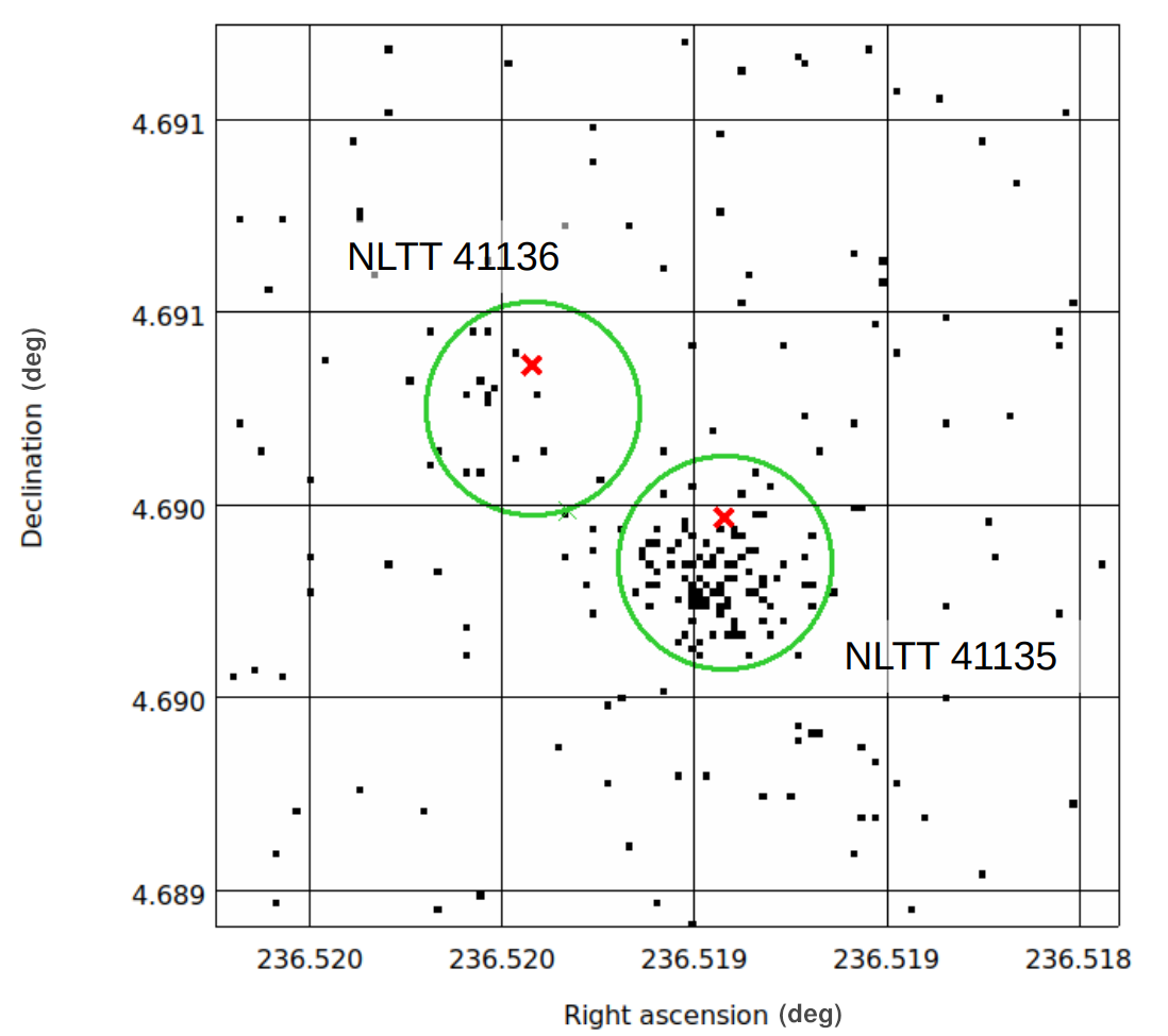
Figure 1: Combined Chandra/HRC-I observations of the system NLTT 41135/41136 with source extraction regions as green circles and the Gaia eDR3 coordinates, propagated to the epoch of observation, as red x-symbols.

The light curve obtained from the observation conducted in October shows a flare occurring on NLTT 41135 at $\approx$ 20 ks after the start of the observation (see Figure 2). We estimated the quiescent X-ray flux by excluding the photon counts occurring in the time interval of the flare, but we also calculated the emission parameters from the whole observation time. In general, when further commenting on the activity difference between the NLTT 41135/41136 stellar components, we will be referring to the comparison of the quiescent components of the coronae. When referring to the emission with the flaring event, we will explicitly state it.

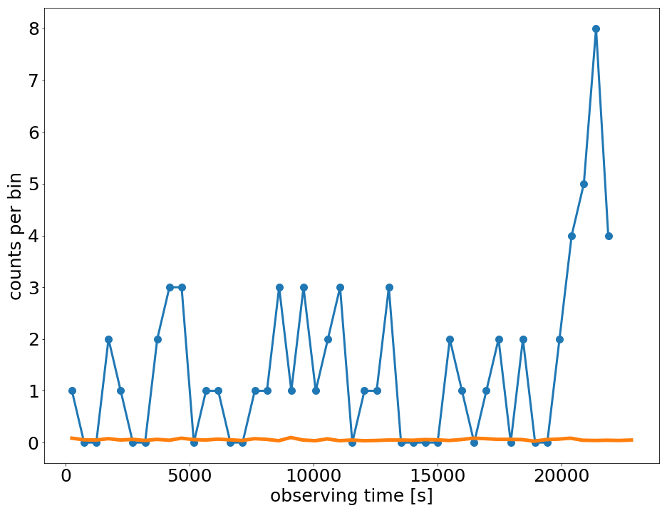
Figure 2: X-ray light curve of NLTT 41135 obtained from observation 26143. The blue dots show the count number with 500 s binsize, while the orange line shows the level of scaled background counts. At 20 ks after the observation start, a flare occurred.

2.3 Net source photon count

In general, to determine the net source photon count of a faint source, both the Poissonian uncertainties of the source and the background need to be taken into account. For the analysis of the two stars from the NLTT 41135/41136 system, we employed the analysis for faint sources described by Ilic et al. (2022). In short, firstly, we estimated the probability that the background fluctuation was responsible for the number of counts in the source region by employing the Poisson cumulative distribution function. For both sources, we found that this probability was lower than 0.3%, securing a $3\sigma$ level of detection significance. Furthermore, to estimate the net source photon count and its confidence interval, we applied the Kraft-Burrows-Nousek (KBN) estimator (Kraft et al., 1991a). The KBN estimator tackles the small number statistics of faint sources in a Bayesian manner by explicitly assuming the background signal stems from a Poisson process and marginalizing over all possible background count numbers in the source detect cell. It assumes the source flux to be non-negative, and yields confidence intervals for the net source photon count. For the two detected sources, we determined the 68.3% confidence interval and reported the number of counts at its center as the net source photon count in Table 1.

Table 1: Observed X-ray emission parameters for the stellar components NLTT 41135 and NLTT 41136. NLTT 41135 flared, and we estimated the parameters with (active) and without (quiescent) the flare.

component	counts	scaled bg counts	net counts	obs time [s]	count rate [cts/s]	$\log_{10}T$ [K]	$F_{x}$ $\mathrm{[erg/s/cm^{2}]}$
NLTT 41136	15	5.556	$9.444_{-3.566}^{+4.240}$	48138	$0.00020_{-0.00007}^{+0.00009}$	$6.3\pm 0.1$	$\left(2.220_{-0.812}^{+0.964}\right)\times 10^{-15}$
NLTT 41135 (quiescent)	85	5.244	$79.762^{+9.565}_{-8.910}$	45078	$0.00177_{-0.00020}^{+0.00021}$	$6.6\pm 0.1$	$\left(1.596_{-0.178}^{+0.192}\right)\times 10^{-14}$
NLTT 41135 (including flare)	106	5.556	$100.449_{-9.983}^{+10.643}$	48138	$0.00209_{-0.00021}^{+0.00022}$		$\left(1.883_{-0.187}^{+0.199}\right)\times 10^{-14}$

2.4 Coronal temperature and X-ray surface flux

By choosing an activity indicator from the X-ray regime, we make use of the fact that unsaturated X-ray emission is a function of stellar rotational rate: as single stars age, their rotation rate decreases, and as a consequence, their coronal temperature and X-ray emission reduce. However, if a star experiences spin-up, the average coronal temperature of the star increases, and, therefore, a higher X-ray luminosity and surface flux will be observed.

Since the HRC-I has no intrinsic energy resolution, determining the coronal temperature directly from the observed radiation is not possible. A solution to this issue is the employment of a scaling relation between the average coronal temperature and X-ray surface flux for low-mass main-sequence stars. Observations with various X-ray telescopes have shown that the X-ray surface flux and the coronal temperature of stellar coronae are closely correlated (Schmitt, 1997; Johnstone & Güdel, 2015; Magaudda et al., 2022).

We use here the sample presented by Johnstone & Güdel (2015) to test where in the distribution of X-ray surface fluxes and coronal temperatures our sources would fall when assuming different coronal temperatures on a test grid. A caveat with this approach is that the coronae of M dwarfs can have multiple thermal components (Schmitt et al., 1990; Giampapa et al., 1996; Robrade & Schmitt, 2005), but having no spectral information of the observed coronae only allowed us to estimate the mean coronal temperature.

Inspired by the methodology presented by Ayres & Buzasi (2022), we used the online tool webpimms (v4.12a) to calculate expected fluxes, for given count rate, for a test grid of coronal temperatures ranging from $\log_{10}T\mathrm{[K]}=6.0-7.0$ with 0.1 dex stepsize. The elemental abundances were set to 0.4 of the solar abundance, as suggested by Irwin et al. (2010), since NLTT 41135/41136 belongs to the old galactic disk population where the usual abundance is subsolar (Leggett, 1992). The temperature uncertainty is set to be equal to the stepsize of the temperature grid and influences the flux uncertainty much less than the photon count uncertainty provided in Table 1.

Using the resulting X-ray flux and the known distance to the system (Bailer-Jones et al., 2018), we calculated the stellar X-ray luminosity. By normalizing the luminosity with the optical surface area of the star, we arrive at the stellar X-ray surface flux value. We then compared the coronal temperature – X-ray surface flux pairs to the sample from Johnstone & Güdel (2015), which is shown in Figure 3. We chose the pair that matches the Johnstone sample best and proceeded with those values as our best estimates for the coronal temperature and X-ray surface flux, as given in Table 1.

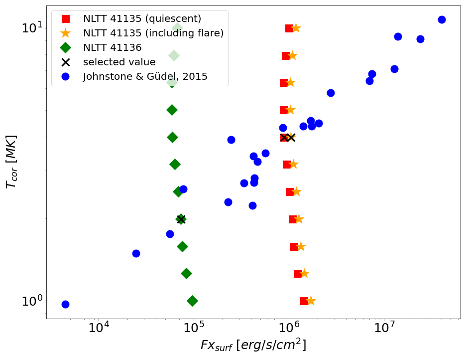
Figure 3: Coronal temperature vs. X-ray surface flux from Johnstone & Güdel (2015) with blue dots, and the grid calculated for our targets: for NLTT 41136 with green diamond, and for NLTT 41135 with red squares and orange stars for quiescent and overall emission, respectively.

The flux confidence interval was estimated by using the limits of the $1\sigma$ confidence interval of the net source photon count for our sources and applying these values in the webpimms tool with the coronal temperature estimated in the previous step. The resulting flux values were used as the upper and lower limits of the $1\sigma$ uncertainty of the X-ray flux. With error propagation, we used the estimated X-ray flux uncertainty to estimate the X-ray luminosity and -surface flux uncertainty. The distance uncertainty was not taken into account for error propagation since it is less than 1%.

2.5 Stellar radii

Before we are able to calculate the X-ray surface flux, we needed an estimate of the stellar radius. Usually, the radii of M dwarf stars are estimated by applying the empirical relation between the Ks-band magnitude of a star and its radius, published by Mann et al. (2015). However, the NLTT 41135/41136 system, together with several systems from the control sample, does not have a published detection in the Ks band for both components. Therefore, to have uniformly estimated stellar radii for all stars, we estimate the absolute magnitude of a star and use the main-sequence parameters published by Pecaut & Mamajek (2013). We employ the photometric measurement made by the ESA Gaia mission (Gaia Collaboration et al., 2016, 2018) and geometric distances to the stars (Bailer-Jones et al., 2018) to calculate the absolute G magnitude. We then estimate the stellar radius for each star by interpolating the stellar radius vs. absolute G magnitude function for main-sequence stars for the observed magnitude. In Table 2, we give the distance, Gaia photometry, and calculated radii of all stars in our sample: the NLTT 41135/41136 system, and the control binary systems (see Section 3.2).

For GJ 65, one of the control systems, the radii estimated from interferometric measurements of the stars’ angular diameters (Kervella et al., 2016) were available as well. We also estimate the stellar radii for this system and find a discrepancy of $\approx 10\%$ between the interferometric and our values. This is not that surprising since it was found that stellar evolutionary models, by using photometric measurements, underestimate the stellar radius of M dwarfs (Ribas, 2006; Torres, 2013). Since we are interested in the flux ratio of binary stars, we expect that, to the first order, the effect of radius discrepancy between real and model values will cancel out and will not significantly impact the final result.

3 Results

3.1 The X-ray properties of NLTT 41135/41136

Although the two M dwarfs in this system have similar stellar parameters, their coronal activity levels differ greatly. Firstly, from the inspection of the X-ray light curve obtained from the observation with ID 26143, a flaring event on NLTT 41135 took place towards the end. On the other hand, the primary NLTT 41136 does not show any evidence of flaring for the entire 50 ks of the observation. The quiescent count rate and the estimated average coronal temperature of the two components indicate a similar conclusion: the secondary has a count rate of $\mathrm{1.8\times 10^{-3}}$ count/s and a coronal temperature of $\log_{10}T\mathrm{[K]}$ = 6.6, while the primary has an order of magnitude lower count rate of $\mathrm{2\times 10^{-4}}$ count/s and a lower temperature of $\log_{10}T\mathrm{[K]}$ = 6.3 (see Table 1 for more details). Finally, by comparing the X-ray surface fluxes of the two stars, we establish the significant difference in activity between the two stars: the brown dwarf-hosting star, NLTT 41135 with $F\mathrm{x_{surf}}=8.9\times 10^{5}$ $\mathrm{erg/s/cm^{2}}$, shows more than an order of magnitude greater X-ray surface flux than the primary NLTT 41136, which has a flux of $F\mathrm{x_{surf}}=7.2\times 10^{4}$ $\mathrm{erg/s/cm^{2}}$ (see Table 3 for more details).

3.2 M dwarf wide binary systems for activity difference comparison

To determine the significance of the measured coronal activity difference between NLTT 41135 and NLLT 41136, and, therefore, the tidal influence of the brown dwarf, we constructed a comparison sample of wide M dwarf binaries without known close-in substellar companions. We searched the El-Badry & Rix (2018) wide stellar binaries catalog for M dwarf pairs that harbor stars with similar Gaia $G-G_{\mathrm{RP}}$ color. We selected pairs where the absolute value of the color difference is $|d(G-G_{\mathrm{RP}})|\leq 0.2$, i.e. where the stellar components can differ by up to three spectral subtypes. We expect that coeval M dwarfs with colors differing by more than the equivalent of three spectral subtypes will follow somewhat different stellar evolutionary paths, leading the stars to display noticeably different activity levels in the X-ray regime. This scenario might be true for some coeval stars differing by $|d(G-G_{\mathrm{RP}})|\leq 0.2$; however, the selected color-difference limit is a compromise between having a significant number of systems for comparison and them having intrinsically different stars. Aside from the color-difference constraint, we also imposed a constraint on the distance to the systems since most moderately active M dwarfs will not be detected in routine X-ray observations at larger distances. Below, we describe the query for M dwarf pairs in the source catalogs and data archives of three X-ray space observatories: the XMM-Newton space telescope, the Chandra X-ray Observatory, and the eROSITA instrument onboard the Spectrum Röntgen Gamma satellite.

3.2.1 XMM-Newton

To find M dwarf pairs observed with XMM-Newton’s European Photon Imaging Camera (EPIC), we used input pairs from the El-Badry & Rix (2018) sample as described above and considered pairs within a distance of 100 pc and where the two stars have a separation of at least $15\arcsec$, since stars at closer separation are typically spatially blended in EPIC observations. We used the 4XMM-DR10 catalog, version 1.0 (Webb et al., 2020) for cross-matching. Since XMM-Newton observations have been conducted since 1999 and several of our nearby input pairs display significant proper motions, we first searched for potential matches between the El-Badry & Rix (2018) sample with coordinates evolved to the J2010.0 epoch and the XMM-Newton catalog with a large matching radius of 30″. We then extracted the actual observational epoch(s) from the XMM-Newton catalog, evolved the stellar coordinates to that specific epoch, or in case of multiple XMM-Newton observations to the average epoch, and refined the cross-match by using a matching radius of $5\arcsec$ with the updated coordinates. A visual inspection of the resulting matches in ESASky showed that for some pairs there was source confusion present, especially when the targets were located at the edge of the EPIC field of view. We, therefore, proceeded by downloading the individual observational data sets from the XMM-Newton archive and performed a customized analysis by hand.

The query of the 4XMM-DR10 catalog resulted in 10 M dwarf systems. One of these systems, BX Tri, is a hierarchical system hosting a tight pair that was not flagged as such in the El-Badry & Rix (2018) catalog, and which is not spatially resolved by XMM-Newton. We analysed the observations of the remaining nine systems, obtained from the XMM-Newton data archive, as described by Ilic et al. (2022), and find six systems where both components are detected, and three systems where one component is not detected. We report the fluxes of the detected M dwarfs, and the upper limits of the undetected ones in Table 3. There, the flux values are given for the energy range of 0.2-2.0 keV, where stellar coronae typically emit the bulk of their radiation (Güdel et al., 1997). The values of the X-ray fluxes are computed assuming an underlying thermal spectrum with a coronal temperature estimated from the observed hardness ratio, as described in more detail by (Ilic et al., 2022, see Appendix B for the details on individual systems).

3.2.2 Chandra

The Chandra X-ray observatory has a higher spatial resolution, but generally lower sensitivity than XMM-Newton. We, therefore, selected M dwarf pairs with a spatial separation of at least 2″and within a distance of 50 pc from the El-Badry & Rix (2018) sample and cross-matched them with the Chandra Source Catalog 2.0 (CSC2.0, Evans & Civano 2018) in a similar manner as we did for the XMM-Newton. Again, since Chandra has been in operation since 1999, we used stellar coordinates evolved to an epoch of J2010.0 for initial cross-matching with a matching radius of 30″. We then directly proceeded by downloading the individual observation files from the Chandra archive and performed source detection analysis as described by Ilic et al. (2022). We found two systems where both components are detected, three systems where no component was detected, and three systems where one component is not detected; for all undetected stars, we again report the one-sided $3\sigma$ confidence interval as the upper limit on the X-ray flux. Out of those eight systems, all but one were observed with the ACIS instrument, and we estimated energy conversion factors as described by Ilic et al. (2022) from hardness ratios and reported X-ray fluxes in the 0.2-2.0 keV energy band. For the one system that was observed with the HRC instrument, we perform the same analysis as described in section 2.4 for the NLTT41135/41136 system to find its X-ray flux in the full HRC energy band of 0.08-10 keV. In Appendix B we provide more details on individual systems together with the observed radiation hardness ratio and estimated coronal temperature used for the X-ray flux calculation.

We also added the known binary system GJ 65 to the control sample, which was not included in the wide stellar binary catalog by El-Badry & Rix (2018). A detailed analysis of the two recent observations (obs ID: 22344 and 22876) is performed by Wolk et al. (in prep) and the resulting fluxes are included here. The X-ray photometry of M dwarfs observed with Chandra is reported in Table 3.

3.2.3 eROSITA M dwarf pairs

We compared the selected M dwarf wide binaries from the catalog described above to the catalog of X-ray sources detected with the Röntgen Survey with an Imaging Telescope Array (eROSITA) (Merloni et al., 2012; Freyberg et al., 2020; Dennerl et al., 2020; Predehl et al., 2021; Brunner et al., 2022), an X-ray instrument onboard the Russian Spectrum-Röntgen-Gamma spacecraft (Sunyaev et al., 2021; Pavlinsky et al., 2021). It was launched in mid-2019 into an orbit around the $\mathrm{L_{2}}$ Lagrange point of the Sun-Earth system. eROSITA consists of seven Wolter telescopes with one camera assembly each and is sensitive to photon energies between 0.2-10 keV (Meidinger et al., 2020). eROSITA started an all-sky survey in 2019, where it scans the whole sky every six months in great circles roughly perpendicular to the ecliptic. Any point on the sky is scanned every four hours for several eROSITA slews, with the number of slews when a given target is in the field of view depending on the ecliptic latitude of the target.

eROSITA has completed four all-sky surveys to date (named eRASS1 to eRASS4), as well as a partially-completed fifth all-sky survey (eRASS5). In addition to source catalogs from each of those surveys, the eROSITA_DE consortium has also produced a catalog from the stacked data of the four completed eRASS surveys in the German part of the eROSITA sky, called eRASS:4, accessible within the eROSITA consortium in the data reduction version from October 31 2022. eROSITA has wide wings of its PSF; to avoid issues with source blending and upper limit calculations, we selected known M dwarf binary pairs within a volume of 50 pc that have a separation of at least $50\arcsec$ between the two stars. We then matched those individual stars to the catalog with a matching radius of $10\arcsec$ and checked that all matched X-ray sources are likely to be of stellar nature, as described by Foster et al. (2022).

The stacked eRASS:4 survey (as well as the individual eRASS surveys) is shallow, with total exposure times of the order of 500 s. M dwarfs frequently produce X-ray flares, which increases the probability that some of the M dwarf detections in eRASS:4 were only achieved because the M dwarf flared during the exposure time. Indeed, there is evidence of this reported in Stelzer et al. (2022). Since we want to compare the quiescent X-ray emission levels of stars, we therefore clean the initially matched sample as follows: we require that a given star, in addition to being detected in the stacked eRASS:4 survey, is detected in at least three of the five individual eRASS1 to eRASS5 surveys, meaning we have likely seen the quiescent emission from the star. We then estimate the quiescent flux of the star by taking the median of the individually detected flux values, and its uncertainty by the standard deviation of those detected individual fluxes. We note that three detections is the minimum number required to identify one outlier and determine the typical flux via the median.

Systems in which fewer than three flux detections were achieved were considered to be dominated by flaring emission and, since we do not have a way to characterize the quiescent flux from the available data, they were discarded. Systems in which one star had a detected quiescent flux as described above, but the other star had no detection, were kept in the sample and an upper limit to the flux of the undetected star was computed using the prescription of Tubín-Arenas et al. 2023 (submitted), i.e. by performing X-ray photometry on the eROSITA standard calibration data products (counts image, background image, and exposure time), following the Bayesian approach described by Kraft et al. (1991b). The upper limits are given as one-sided $3\sigma$ confidence intervals in the eROSITA soft band, which has an energy range of 0.2-2.3 keV, and using appropriate energy conversion factors for a stellar corona with a temperature of $kT=0.3$ keV, typical for moderately active stars (Schmitt et al., 1990; Foster et al., 2022). This procedure yielded ten pairs where both stars have a detected quiescent flux and five pairs where one star has a detected quiescent flux and the other star has an upper limit.

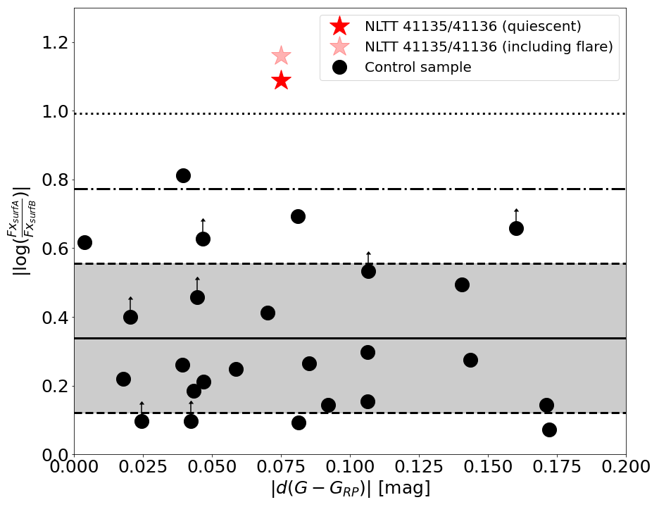
Figure 4: The activity difference as a function of the absolute value of color difference, which corresponds to the mass difference between the components of the wide binary. The binary systems from the control sample are shown as black dots and the NLTT 41135/41136 system as the red asterisk symbol, with the fainter red asterisk including the flaring episode. The solid black line is the mean of the activity difference of the control sample, the shaded area indicates the $1\sigma$ confidence interval around the mean, while the dashed and dotted lines represent the $+2\sigma$ and $+3\sigma$ confidence interval limits, respectively.

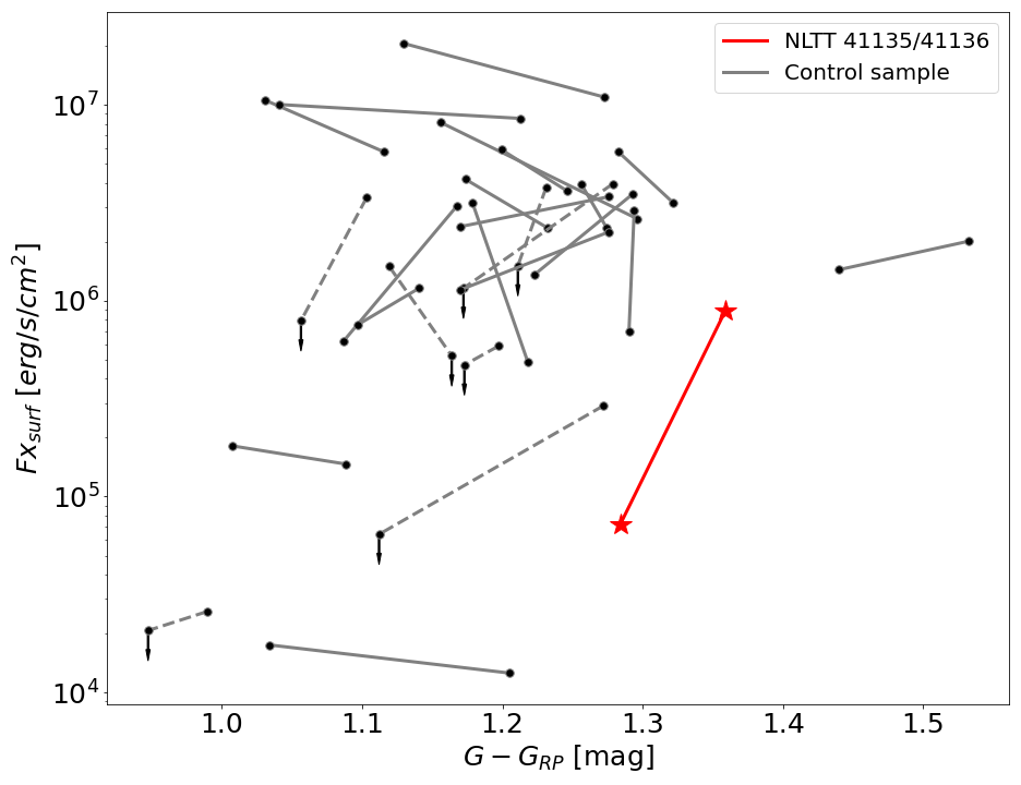
Figure 5: The X-ray surface flux as a function of the Gaia color of M dwarfs in the control sample and the NLTT 41135/41136 system. The two components of a binary are connected with a line: the gray solid line shows binaries where both components are detected, the gray dashed line shows systems where one component is undetected, and the red line connects NLTT 41135 and NLTT 41136.

Table 2: Spectral type (SpT) and projected physical separation ($\rho$) of the components together with their Gaia DR2 photometry and distances (Bailer-Jones et al., 2018) used to calculate the absolute G magnitudes and the radii. Additionally, the absolute value of the color difference between the binary components and their Gaia DR2 stellar proper motion, used to evolve coordinates to a certain epoch, are given.

component	SpT	$\rho$ [AU]	dist [pc]	G	$G-G_{RP}$	$M_{G}$	$R_{Gaia}[R_{\odot}]$	$|d(G-G_{RP})|$	$\mu_{\alpha}\cdot\cos\delta$[mas/yr]	$\mu_{\delta}$[mas/yr]
NLTT 41136	M4	79	34.319	13.966	1.284	11.289	0.269	0.075	$153.670\pm 0.243$	$-281.981\pm 0.241$
NLTT 41135	M5		34.136	14.936	1.359	12.270	0.205		$162.509\pm 0.182$	$-282.725\pm 0.182$
GJ 15 B	M3	122	3.561	9.677	1.205	11.919	0.225	0.171	$2863.284\pm 0.069$	$336.529\pm 0.039$
GJ 15 A	M1		3.562	7.216	1.034	9.458	0.435		$2891.525\pm 0.061$	$411.903\pm 0.034$
Gaia DR2 1608710752684301312	M4	4908	74.594	15.646	1.294	11.283	0.269	0.004	$-27.898\pm 0.095$	$30.127\pm 0.084$
Gaia DR2 1608710791338814208	M4		75.330	16.155	1.290	11.770	0.236		$-29.958\pm 0.103$	$29.634\pm 0.085$
Ross 868	M3	181	10.751	10.137	1.170	9.980	0.372	0.106	$-214.777\pm 0.077$	$351.001\pm 0.084$
Ross 867	M4		10.753	11.456	1.276	11.298	0.268		$-226.132\pm 0.098$	$355.284\pm 0.105$
TIC 293303829	M1	4576	55.871	12.230	1.019	8.494	0.538	0.023	$-24.591\pm 0.117$	$-167.143\pm 0.057$
TIC 293303832	M0		55.853	12.063	0.996	8.328	0.562		$-24.573\pm 0.095$	$-166.795\pm 0.046$
Gaia DR2 3074577322667614976	M3	17201	53.705	13.730	1.199	10.080	0.359	0.047	$-43.033\pm 0.092$	$-86.589\pm 0.065$
Gaia DR2 3074630580262065536	M4		53.625	14.777	1.246	11.130	0.280		$-42.529\pm 0.106$	$-86.487\pm 0.066$
TIC 436632332	M4	2176	83.799	14.970	1.282	10.353	0.338	0.039	$19.706\pm 0.148$	$-43.233\pm 0.086$
TIC 436632331	M4		83.769	14.970	1.322	10.355	0.338		$20.083\pm 0.141$	$-43.467\pm 0.083$
Gaia DR2 4768120070358120064	M4	3219	91.156	16.887	1.272	12.088	0.215	0.16	$37.732\pm 0.156$	$11.151\pm 0.182$
Gaia DR2 4768120104717857792	M2		91.011	14.854	1.112	10.058	0.360		$37.515\pm 0.078$	$10.981\pm 0.099$
G 202-66	M3	1526	60.676	13.395	1.179	9.480	0.433	0.039	$-239.59\pm 0.058$	$174.561\pm 0.064$
G 202-67	M3		60.676	15.046	1.218	11.131	0.280		$-241.61\pm 0.072$	$175.549\pm 0.089$
LTT 6326	M0	1640	61.690	12.796	0.990	8.845	0.498	0.042	$-55.483\pm 0.037$	$-334.752\pm 0.042$
LTT 6325	M0		61.774	12.397	0.948	8.443	0.544		$-55.444\pm 0.038$	$-333.655\pm 0.042$
LP320-163	M6	102	45.653	16.098	1.447	12.801	0.180	0.032	$-212.555\pm 0.155$	$27.959\pm 0.12$
LP320-162	M5		46.370	16.152	1.416	12.821	0.180		$-218.427\pm 0.153$	$28.591\pm 0.118$
LP920-61 B	M3	87	18.234	12.506	1.197	11.202	0.275	0.024	$-121.425\pm 0.105$	$-122.807\pm 0.075$
LP920-61 A	M3		18.268	12.450	1.173	11.141	0.279		$-113.453\pm 0.106$	$-123.013\pm 0.075$
SCR J0602-3952-B	M3	126	45.719	14.274	1.232	10.973	0.292	0.054	$75.063\pm 0.073$	$178.107\pm 0.07$
SCR J0602-3952-A	M3		45.885	13.436	1.178	10.127	0.355		$72.687\pm 0.051$	$175.841\pm 0.049$
TIC 20446899	M0	1778	40.659	11.402	0.969	8.356	0.557	0.184	$-170.787\pm 0.093$	$4.69\pm 0.068$
Gaia DR2 3532611086293698560	M3		40.566	13.127	1.152	10.086	0.358		$-172.895\pm 0.096$	$7.383\pm 0.066$
G236-1	M2	1054	11.850	9.563	1.097	9.195	0.457	0.043	$-671.954\pm 0.045$	$-271.231\pm 0.058$
G236-2	M3		11.873	10.067	1.141	9.695	0.417		$-671.125\pm 0.055$	$-265.525\pm 0.062$
Gaia DR2 715928515183511040	M4	387	36.055	14.404	1.275	11.619	0.246	0.118	$4.986\pm 0.101$	$53.474\pm 0.096$
TIC 16151129	M3		35.905	12.839	1.157	10.063	0.360		$3.271\pm 0.08$	$58.59\pm 0.07$
Ross 110 B	M4	68	21.557	13.196	1.262	11.529	0.252	0.014	$544.582\pm 0.062$	$-549.415\pm 0.062$
Ross 110 A	M4		21.479	12.904	1.248	11.244	0.272		$547.56\pm 0.125$	$-535.855\pm 0.119$
GJ 65 A	M6	6	2.703	10.507	1.440	13.348	0.156	0.092	$3385.827\pm 0.492$	$532.040\pm 0.374$
GJ 65 B	M7		2.687	10.869	1.532	13.723	0.148		$3182.734\pm 0.552$	$592.104\pm 0.427$

Table 2: Continued

component	SpT	$\rho$ [AU]	dist [pc]	G	$G-G_{RP}$	$M_{G}$	$R_{Gaia}[R_{\odot}]$	$|d(G-G_{RP})|$	$\mu_{\alpha}\cdot\cos\delta$[mas/yr]	$\mu_{\delta}$[mas/yr]
TIC 206617096	M4	18438	34.690	14.375	1.274	11.674	0.242	0.018	$1.598\pm 0.077$	$84.663\pm 0.075$
TIC 206617113	M4		34.703	14.168	1.257	11.467	0.256		$1.177\pm 0.063$	$85.017\pm 0.056$
GJ 3148	M3	1415	13.408	10.777	1.174	10.140	0.354	0.059	$684.129\pm 0.127$	$248.772\pm 0.103$
GJ 3149	M3		13.433	11.749	1.232	11.108	0.282		$683.716\pm 0.161$	$246.394\pm 0.134$
UCAC4 235-004550	M1	2601	39.520	11.739	1.031	8.755	0.508	0.085	$35.9\pm 0.043$	$-33.357\pm 0.061$
UCAC4 235-004546	M2		39.551	12.384	1.116	9.398	0.439		$37.114\pm 0.048$	$-32.231\pm 0.078$
Gaia DR2 4899032116649119616	M4	13801	38.939	14.766	1.269	11.814	0.233	0.121	$-28.019\pm 0.073$	$-45.644\pm 0.077$
Gaia DR2 4899029951985608576	M5		39.098	16.142	1.391	13.181	0.164		$-28.182\pm 0.109$	$-46.464\pm 0.113$
TIC 167422188	M1	13368	40.774	11.890	1.007	8.839	0.499	0.081	$79.093\pm 0.048$	$234.317\pm 0.046$
TIC 167417695	M2		41.058	12.628	1.089	9.561	0.428		$78.676\pm 0.053$	$233.277\pm 0.054$
TIC 106344480	M1	45353	24.390	10.606	1.041	8.670	0.518	0.172	$37.481\pm 0.038$	$-34.252\pm 0.039$
TIC 106493402	M3		24.466	12.216	1.213	10.274	0.344		$36.45\pm 0.051$	$-31.75\pm 0.067$
TIC 416857959	M2	5204	39.125	12.356	1.103	9.393	0.439	0.047	$-36.339\pm 0.051$	$47.232\pm 0.054$
TIC 450297524	M1		39.122	12.097	1.056	9.135	0.464		$-36.251\pm 0.051$	$48.66\pm 0.048$
TIC 36765037	M3	2631	30.149	13.589	1.231	11.192	0.275	0.02	$-183.1\pm 0.462$	$-26.428\pm 0.697$
TIC 36765044	M3		31.660	13.626	1.211	11.124	0.281		$-182.39\pm 0.152$	$-25.195\pm 0.129$
TIC 151639642	M2	3799	36.792	12.031	1.087	9.202	0.456	0.081	$31.746\pm 0.043$	$-79.325\pm 0.045$
UCAC4 270-056947	M3		36.838	12.738	1.168	9.906	0.384		$31.723\pm 0.049$	$-78.358\pm 0.05$
UCAC4 150-081944	M4	6132	30.374	14.268	1.296	11.855	0.230	0.14	$-145.97\pm 0.097$	$-64.886\pm 0.08$
TIC 317385747	M3		30.317	12.357	1.156	9.949	0.377		$-147.448\pm 0.054$	$-66.219\pm 0.047$
TIC 392786054	M3	9659	26.342	12.641	1.223	10.538	0.325	0.07	$159.768\pm 0.113$	$-83.222\pm 0.098$
TIC 392785968	M4		26.445	13.618	1.293	11.506	0.254		$160.361\pm 0.124$	$-82.213\pm 0.098$
WT 2090	M4	5413	21.426	13.371	1.279	11.716	0.239	0.107	$-171.652\pm 0.125$	$-247.082\pm 0.11$
Wolf 1501	M3		21.408	12.113	1.172	10.461	0.330		$-170.941\pm 0.093$	$-247.728\pm 0.081$
TIC 410458113	M2	4370	27.554	11.787	1.119	9.586	0.427	0.045	$88.314\pm 0.119$	$-98.339\pm 0.082$
UCAC4 385-070621	M3		27.579	12.656	1.164	10.453	0.331		$89.838\pm 0.121$	$-95.569\pm 0.082$
TIC 229807000	M2	35099	45.987	11.983	1.129	8.670	0.518	0.144	$73.503\pm 0.041$	$-68.137\pm 0.042$
TIC 229807051	M4		45.885	13.875	1.273	10.566	0.323		$73.624\pm 0.071$	$-68.011\pm 0.071$

Table 3: X-ray parameters for all the stars in our sample, together with the activity difference in each binary. Additionally, we provide the instrument with which Chandar systems were observed; XMM-Newton systems were observed only with the EPIC instrument.

mission	component	$F_{x}\times 10^{-14}$ $[erg/s/cm^{2}]$	$L_{x}\times 10^{27}$ [erg/s]	$Fx_{surf}\times 10^{5}$ $[erg/s/cm^{2}]$	$L_{bol}\times 10^{31}$ [erg/s]	$\log R_{x}$	$\left|\log\frac{Fx_{surfA}}{Fx_{surfB}}\right|$
Chandra/HRC	NLTT 41136	$0.22\pm 0.09$	$0.32\pm 0.13$	$0.72\pm 0.29$	2.61	-4.91	$1.09\pm 0.18$
	NLTT 41135 (quiescent)	$1.6\pm 0.2$	$2.3\pm 0.3$	$8.9\pm 1.0$	$1.31\times 10^{31}$	-3.76
	NLTT 41135 (average)	$1.9\pm 0.2$	$2.7\pm 0.3$	$10.0\pm 1.0$		-3.69	$1.16\pm 0.18$
XMM-Newton	GJ 15 B	$2.506\pm 0.136$	$0.04\pm 0.0$	$0.13\pm 0.01$	$1.67$	-5.63	$0.14\pm 0.03$
	GJ 15 A	$12.992\pm 0.285$	$0.2\pm 0.0$	$0.17\pm 0.0$	$10.02$	-5.70
XMM-Newton	Gaia DR2 1608710752684301312	$1.88\pm 0.144$	$12.76\pm 0.98$	$29.0\pm 2.23$	$2.64$	-3.32	$0.62\pm 0.09$
	Gaia DR2 1608710791338814208	$0.341\pm 0.068$	$2.36\pm 0.47$	$7.0\pm 1.39$	$1.86$	-3.90
XMM-Newton	Ross 868	$67.726\pm 0.802$	$9.55\pm 0.11$	$11.34\pm 0.13$	$6.65$	-3.84	$0.3\pm 0.01$
	Ross 867	$69.566\pm 0.815$	$9.81\pm 0.11$	$22.47\pm 0.26$	$2.62$	-3.43
XMM-Newton	TIC 293303829	$0.178\pm 0.055$	$0.68\pm 0.21$	$0.38\pm 0.12$	$19.86$	-5.47	/
	TIC 293303832	$\leq 0.451$	$\leq 1.72$	$\leq 0.89$	$22.85$	$\leq-5.12$
XMM-Newton	Gaia DR2 3074577322667614976	$13.115\pm 0.219$	$46.14\pm 0.77$	$58.93\pm 0.98$	$6.11$	-3.12	$0.21\pm 0.02$
	Gaia DR2 3074630580262065536	$4.934\pm 0.152$	$17.31\pm 0.53$	$36.26\pm 1.12$	$2.96$	-3.23
XMM-Newton	TIC 436632332	$4.698\pm 0.272$	$40.25\pm 2.33$	$57.77\pm 3.34$	$5.08$	-3.10	$0.26\pm 0.04$
	TIC 436632331	$2.582\pm 0.197$	$22.1\pm 1.69$	$31.75\pm 2.42$	$5.08$	-3.36
XMM-Newton	Gaia DR2 4768120070358120064	$0.08\pm 0.021$	$0.82\pm 0.21$	$2.91\pm 0.76$	$1.48$	-4.26	$\geq 0.66$
	Gaia DR2 4768120104717857792	$\leq 0.05$	$\leq 0.51$	$\leq 0.64$	$6.2$	$\leq-5.09$
XMM-Newton	G 202-66	$7.999\pm 0.3$	$35.92\pm 1.35$	$31.43\pm 1.18$	$9.88$	-3.44	$0.81\pm 0.08$
	G 202-67	$0.514\pm 0.093$	$2.31\pm 0.42$	$4.84\pm 0.88$	$2.96$	-4.11
XMM-Newton	LTT 6326	$0.084\pm 0.027$	$0.39\pm 0.12$	$0.26\pm 0.08$	$15.39$	-5.60	$\geq 0.1$
	LTT 6325	$\leq 0.08$	$\leq 0.37$	$\leq 0.21$	$20.61$	$\leq-5.74$
Chandra/ACIS	LP 320-163	$0.098\pm 0.109$	$0.25\pm 0.28$	$1.25\pm 1.4$	$0.91$	-4.57	/
	LP 320-162	$\leq 0.564$	$\leq 1.48$	$\leq 7.55$	$0.9$	$\leq-3.78$
Chandra/ACIS	LP 920-61 B	$6.634\pm 2.549$	$2.69\pm 1.03$	$5.87\pm 2.25$	$2.8$	-4.02	$\geq 0.1$
	LP 920-61 A	$\leq 5.474$	$\leq 2.23$	$\leq 4.7$	$2.93$	$\leq-4.12$
Chandra/ACIS	SCR J0602-3952-B	$\leq 0.255$	$\leq 0.65$	$\leq 1.25$	$3.32$	$\leq-4.71$	/
	SCR J0602-3952-A	$\leq 0.342$	$\leq 0.88$	$\leq 1.15$	$5.92$	$\leq-4.83$
Chandra/ACIS	Ross 868	$142.48\pm 6.377$	$20.09\pm 0.9$	$23.86\pm 1.07$	$6.65$	-3.52	$0.15\pm 0.03$
	Ross 867	$105.183\pm 6.508$	$14.84\pm 0.92$	$33.97\pm 2.1$	$2.62$	-3.25
Chandra/ACIS	TIC 20446899	$0.018\pm 0.007$	$0.04\pm 0.01$	$0.02\pm 0.01$	$22.28$	-6.79	/
	Gaia DR2 3532611086293698560	$\leq 0.076$	$\leq 0.15$	$\leq 0.2$	$6.09$	$\leq-5.60$
Chandra/HRC	G236-1	$56.11\pm 2.026$	$9.61\pm 0.35$	$7.56\pm 0.27$	$11.91$	-4.09	$0.18\pm 0.02$
	G236-2	$71.16\pm 2.281$	$12.24\pm 0.39$	$11.56\pm 0.37$	$8.62$	-3.85
Chandra/ACIS	Gaia DR2 715928515183511040	$\leq 1.464$	$\leq 2.32$	$\leq 6.31$	$2.07$	$\leq-3.95$	/
	TIC 16151129	$\leq 1.076$	$\leq 1.69$	$\leq 2.15$	$6.18$	$\leq-4.56$
Chandra/ACIS	Ross 110 B	$\leq 0.235$	$\leq 0.13$	$\leq 0.34$	$2.21$	$\leq-5.22$	/
	Ross 110 A	$\leq 0.189$	$\leq 0.11$	$\leq 0.24$	$2.72$	$\leq-5.41$

Table 3: continued

mission	component	$F_{x}\times 10^{-14}$ $[erg/s/cm^{2}]$	$L_{x}\times 10^{27}$ [erg/s]	$Fx_{surf}\times 10^{5}$ $[erg/s/cm^{2}]$	$L_{bol}\times 10^{31}$ [erg/s]	$\log R_{x}$	$\left|\log\frac{Fx_{surfA}}{Fx_{surfB}}\right|$
Chandra/HRC	GJ 65 A	$268.0\pm 5.6$	$2.39\pm 0.05$	$14.4\pm 0.3$	0.62	-3.41	$0.14\pm 0.02$
	GJ 65 B	$351.5\pm 7.9$	$3.10\pm 0.07$	$20.1\pm 0.4$	0.52	-3.22
eROSITA	TIC 206617096	$5.721\pm 0.339$	$8.4\pm 0.5$	$23.55\pm 1.4$	$1.99$	-3.38	$0.22\pm 0.03$
	TIC 206617113	$10.637\pm 0.574$	$15.63\pm 0.84$	$39.09\pm 2.11$	$2.32$	-3.17
eROSITA	GJ 3148	$145.246\pm 1.889$	$31.85\pm 0.41$	$41.72\pm 0.54$	$5.87$	-3.27	$0.25\pm 0.01$
	GJ 3149	$51.654\pm 1.088$	$11.37\pm 0.24$	$23.54\pm 0.5$	$3.01$	-3.42
eROSITA	UCAC4 235-004550	$87.329\pm 0.798$	$166.37\pm 1.52$	$105.83\pm 0.97$	$16.43$	-2.99	$0.27\pm 0.01$
	UCAC4 235-004546	$35.253\pm 0.602$	$67.27\pm 1.15$	$57.42\pm 0.98$	$10.39$	-3.19
eROSITA	Gaia DR2 4899032116649119616	$5.881\pm 0.22$	$10.88\pm 0.41$	$33.08\pm 1.24$	$1.8$	-3.22	/
	Gaia DR2 4899029951985608576	$\leq 27.522$	$\leq 51.32$	$\leq 315.58$	$0.7$	$\leq-2.14$
eROSITA	TIC 167422188	$1.354\pm 0.02$	$2.75\pm 0.04$	$1.81\pm 0.03$	$15.46$	-4.75	$0.09\pm 0.03$
	TIC 167417695	$0.794\pm 0.048$	$1.63\pm 0.1$	$1.46\pm 0.09$	$9.41$	-4.76
eROSITA	TIC 106344480	$225.667\pm 1.148$	$163.76\pm 0.83$	$100.37\pm 0.51$	$17.47$	-3.03	$0.07\pm 0.06$
	TIC 106493402	$84.167\pm 10.925$	$61.45\pm 7.98$	$85.2\pm 11.06$	$5.37$	-2.94
eROSITA	TIC 416857959	$21.059\pm 0.45$	$39.32\pm 0.84$	$33.52\pm 0.72$	$10.42$	-3.42	$\geq 0.63$
	TIC 450297524	$\leq 5.536$	$\leq 10.34$	$\leq 7.89$	$12.44$	$\leq-4.08$
eROSITA	TIC 36765037	$15.775\pm 1.173$	$17.49\pm 1.3$	$37.93\pm 2.82$	$2.82$	-3.21	$\geq 0.4$
	TIC 36765044	$\leq 5.905$	$\leq 7.22$	$\leq 15.08$	$2.97$	$\leq-3.61$
eROSITA	TIC 151639642	$4.742\pm 0.24$	$7.83\pm 0.4$	$6.19\pm 0.31$	$11.84$	-4.18	$0.69\pm 0.04$
	UCAC4 270-056947	$16.486\pm 1.323$	$27.29\pm 2.19$	$30.48\pm 2.45$	$7.11$	-3.42
eROSITA	UCAC4 150-081944	$7.455\pm 0.727$	$8.39\pm 0.82$	$26.14\pm 2.55$	$1.75$	-3.32	$0.49\pm 0.04$
	TIC 317385747	$62.761\pm 0.868$	$70.36\pm 0.97$	$81.42\pm 1.13$	$6.84$	-2.99
eROSITA	TIC 392786054	$10.25\pm 0.548$	$8.68\pm 0.46$	$13.53\pm 0.72$	$4.49$	-3.71	$0.41\pm 0.03$
	TIC 392785968	$16.011\pm 0.35$	$13.66\pm 0.3$	$34.9\pm 0.76$	$2.25$	-3.22
eROSITA	WT 2090	$24.581\pm 0.953$	$13.76\pm 0.53$	$39.54\pm 1.53$	$1.93$	-3.15	$\geq 0.53$
	Wolf 1501	$\leq 13.757$	$\leq 7.69$	$\leq 11.58$	$4.73$	$\leq-3.79$
eROSITA	TIC 410458113	$17.912\pm 0.407$	$16.59\pm 0.38$	$14.99\pm 0.34$	$9.27$	-3.75	$\geq 0.46$
	UCAC4 385-070621	$\leq 3.753$	$\leq 3.48$	$\leq 5.22$	$4.75$	$\leq-4.14$
eROSITA	TIC 229807000	$130.399\pm 1.647$	$336.38\pm 4.25$	$206.17\pm 2.6$	$17.47$	-2.72	$0.28\pm 0.01$
	TIC 229807051	$26.966\pm 0.832$	$69.26\pm 2.14$	$109.43\pm 3.38$	$4.4$	-2.80

3.3 Intrabinary X-ray surface flux difference

Having estimated the X-ray surface flux of NLTT 41135 and NLTT 41136, and of the binaries in the control sample, as a next step, we estimated the coronal activity level difference between the two stars of each binary. The activity difference is calculated as the absolute logarithmic value of the ratio of the stellar X-ray surface fluxes of the two stars. In Table 3, the values of the stellar X-ray surface flux together with the activity difference ratio for each binary are given. The mean coronal activity difference in the X-ray regime between coeval M dwarfs in the control sample is $|\log(F\mathrm{x_{surfA}}/F\mathrm{x_{surfB}})|=0.34\pm 0.22$, with A and B denoting the surface flux of the primary and the secondary component, respectively. This means that, on average, the X-ray surface flux between two coeval M dwarfs can differ by a factor of $2.2\pm 1.7$, which is similar to the intrinsic variability seen in single M dwarf stars in time-averaged X-ray data (Marino et al., 2000; Stelzer et al., 2013; Magaudda et al., 2022). The mean activity difference was calculated including systems where one star is undetected, and for these systems, we consider the activity difference given in Table 3. Since the sample has three systems with components separated by less than 100 AU, which is the lower limit for binary systems to be considered as wide (Desidera & Barbieri, 2007), we tested if a correlation between the activity difference indicator and the spatial separation between coeval stars exists, and found none.

We did not include the following systems in the analysis: TIC 293303829 / TIC 293303832, Gaia DR2 4899032116649119616 / Gaia DR2 4899029951985608576, LP 320-163 / LP 320-162, and TIC 20446899 / Gaia DR2 3532611086293698560. All systems have one undetected stellar component that has an upper limit value higher than the flux of the detected component, due to differences in the exposure times and in the detectors used. This means that the activity difference of each pair is unconstrained. Additionally, we did not include the undetected systems SCR J0602-3952 A/B, Ross 110 A/B, and Gaia DR2 715928515183511040/TIC 16151129, where the activity difference between the components is unconstrained as well.

In Figure 4, the coronal activity difference is shown as a function of the absolute value of the $G-G_{\mathrm{RP}}$ color difference between the stars in each binary. The 68.3% confidence interval of the control sample distribution is marked with the shaded region, and the mean of the distribution is presented as black solid line. The coronal activity level difference between NLTT 41135 and NLTT 41136 is $|\log(F\mathrm{x_{surfA}}/F\mathrm{x_{surfB}})|=1.09\pm 0.18$ and is given as red asterisk symbol. Here, the brown dwarf-hosting M dwarf has an X-ray surface flux more than an order of magnitude higher than that of its stellar companion. Considering the X-ray surface flux of NLTT 41135 calculated including the flare emission, the activity difference rises to $|\log(F\mathrm{x_{surfA}}/F\mathrm{x_{surfB}})|=1.16\pm 0.18$.

4 Discussion

4.1 The activity difference distribution

It is well known that stars of similar mass, but different ages have X-ray emission levels that can differ by several orders of magnitude (see e.g. Güdel 2004 and references therein). When, on the other hand, we consider stars of similar mass and age, as in our control sample, their emission and activity levels should be more consistent. As we have shown, two stars of the same spectral type in a binary will have a certain degree of difference in their activity level, but typically within a factor of two in coronal brightness. This is much smaller than the range observed for differently-aged stars.

This is also shown in Fig. 5, where the distribution of all investigated stars is shown in the X-ray surface flux – Gaia color parameter space. There, individual stars are shown as black dots and those belonging to the same system are connected with a grey line. If both stars are detected, the connecting line is solid, otherwise, the line is dashed, which indicates that the slope of the connecting line is a minimum absolute value. The NLTT system is presented with red asterisks and a red connecting line; here we used the quiescent X-ray surface flux for the BD-hosting star.

The distribution of systems in Fig. 5 shows a spread of more than three orders of magnitude in the X-ray surface fluxes. The stars in our sample, thus, span nearly the full range of X-ray activity levels present in M dwarfs which was recently shown by Caramazza et al. (2023) on a volume-complete sample to range from $<~{}10^{4}~{}\mathrm{erg/s/cm^{2}}$ (corresponding to the X-ray emission of solar coronal holes) to $>~{}10^{7}~{}\mathrm{erg/s/cm^{2}}$ (corresponding to solar cores of active regions and flares). The X-ray activity level of coronally active stars is known to be linked to the stellar rotation rate, which evolves over time. Therefore, our stars likely represent a range of ages. In fact, within a given binary the X-ray surface fluxes of the two components (which can be assumed to be coeval) are similar to each other, and this leads to the low value of the average activity difference in our sample shown in Fig. 4. However, the activity levels of coeval stars are not equal to each other and there are several processes that can be considered as drivers of the activity difference distribution seen in Fig. 4 and 5. In the following, we discuss phenomena like saturated coronal emission, the fully convective boundary, and activity cycles.

4.1.1 Coronal saturation regime

According to various studies, the coronae of cool main-sequence stars can operate in the saturated or unsaturated regime of emission (Pallavicini et al., 1981; Pizzolato et al., 2003; Wright et al., 2011, 2018; Magaudda et al., 2020; Reiners et al., 2022; Magaudda et al., 2022). In the first regime, the X-ray emission reaches a maximum value and does not depend on the stellar rotation rate, while in the latter, the X-ray emission decreases with the increasing rotation period of the star.

To estimate the coronal emission state, we calculated the parameter $\log R_{\mathrm{x}}=\log\frac{L_{\mathrm{x}}}{L_{\mathrm{bol}}}$ for each individual star in our sample. Here, we calculated the bolometric luminosity, similar to the stellar radius in Sec. 2.5, by using the $L_{\mathrm{bol}}$ values for main-sequence stars published by Pecaut & Mamajek (2013), and interpolating them over the absolute G magnitudes given in Table 2. The $\log R_{\mathrm{x}}$ values of individual stars are given in Table 3.

We estimated the saturation limit for M dwarf stars to be $\log R_{\mathrm{x}}~{}=~{}-3.26^{+0.38}_{-0.36}$, by employing the saturation values for different mass bins from Fig. 9b by Magaudda et al. (2022), and estimating the average value for their full mass range. Taking the average lower saturation limit of $\log R_{\mathrm{x}}=-3.62$, we find that 18 of the pairs in our control sample have at least one star in the saturated regime. These high-activity systems are also seen in Fig. 5 with X-ray surface fluxes above $F\mathrm{x_{surf}}\approx 10^{6}\mathrm{erg/s/cm^{2}}$. Having the majority of the control systems in the high-activity regime is most probably due to the fact that we employ archival data, where the probability of detecting active stars is higher than for low-activity stars. Therefore, our control sample is biased toward brighter X-ray stars.

One might argue that the high-activity systems are more likely to have equal surface fluxes for both stars because they are saturated, which is often interpreted to mean that most of their corona is full with X-ray-emitting magnetic structures. Consequently, it is difficult (or impossible) to produce a coronal activity difference of one order of magnitude between two coeval saturated stars. However, the control sample also includes seven low-activity systems (where both M dwarfs have $F\mathrm{x_{surf}}\lesssim 10^{6}\mathrm{erg/s/cm^{2}}$). Unsaturated stars are not expected to have a coronal filling factor near 100%, and thus the coronal activity difference between the two components of such binaries may take larger values than found in highly active, saturated systems. However, we measure for the low-activity stars $|\log(F\mathrm{x_{surfA}}/F\mathrm{x_{surfB})|=0.30}$, lower than the average for all systems. Here, it has to be noted that some low-activity systems have one star undetected and the calculated mean activity difference is a lower limit.

4.1.2 Fully convective boundary

The fully convective boundary occurs in mid-M dwarfs (e.g. Copeland et al. 1970; Chabrier & Baraffe 1997) and is encompassed by the sample selection we made. It is assumed that, due to high opacity in later M dwarfs, efficient energy transport inside the star is possible only through convection and the star becomes fully convective.

While it was expected that the coronal properties might change at this boundary due to a switch in dynamo mode from an $\alpha-\Omega$ dynamo to a different one (e.g. Chabrier & Küker 2006), observations showed that there is no abrupt change in X-ray luminosity or other coronal activity indicators (Stelzer et al., 2013; Wright & Drake, 2016). Rather, changes in coronal properties were found at the very low-mass end of the M dwarf sequence, where the low temperature of the photosphere may start to affect the formation of active regions (Berger et al., 2010; Robrade & Schmitt, 2009; Stelzer et al., 2012; Williams et al., 2014).

In our sample, we have a few pairs that straddle the fully convective boundary. If this boundary is set at the spectral type $\approx$ M4 with the Gaia color of $G-G_{\mathrm{RP}}\approx 1.24$, in eight systems the primary is partially convective while the secondary is fully convective. However, in these systems, the less-massive star has the spectral type M4 and not later. Therefore, we cannot with certainty say that it is a fully convective star, only that it is potentially fully convective. Therefore, any potential effect due to having fully convective stars in our sample might not be present in our sample.

4.1.3 Activity cycles

One aspect of magnetic activity we were not able to account for is the activity cycle of stars in the X-ray regime. It is well established that stars other than the Sun can have these kinds of cycles (Hempelmann et al., 2006; Robrade et al., 2007; Favata et al., 2008; DeWarf et al., 2010; Coffaro et al., 2020); however, activity cycles in saturated stars and stars close to the fully convective boundary seem to be elusive not only in the coronal part of the stellar atmosphere but in the chromosphere as well (Robertson et al., 2013; Fuhrmeister et al., 2023). It is hypothesized that activity cycles in fully convective stars are absent because the efficiency of magnetic braking decreases (e.g. Chabrier & Küker 2006). For saturated stars, activity cycles might be absent because their coronae are fully covered with magnetic X-ray emitting structures leaving no space for additional X-ray emitting regions. In fact, none of the stars with a detected activity cycle is saturated (Drake & Stelzer, in prep.). However, since in the control sample, we have stars that are both unsaturated and partly convective, the existence of X-ray activity cycles cannot be fully excluded, and their contribution to the observed activity difference remains unconstrained.

4.2 The coronal activity level difference between NLTT 41135 and NLTT 41136 and its physical interpretation

The spin evolution of a star with a close-in companion is driven by processes that can have opposite effects: magnetic braking and tidal interactions. While the wind-driven braking slows down the stellar rotation rate, tidal interactions with a close-in companion can induce spin-up via angular momentum transfer if the configuration of the system is such that the orbital rate of the companion is greater than the rotation rate of the star. As a consequence of the spin-up scenario, the star can experience a higher magnetic activity level than would be the case without tidal interactions. To test this hypothesis when the companion is a substellar object, we analysed the subsystem NLTT 41135, a brown dwarf-M dwarf pair, together with their stellar companion NLTT 41136, which is expected to have the baseline activity level which is governed only by magnetic braking.

Since, in general, a difference in activity between coeval stars with the same spectral type should be expected, we introduced a control sample which showed that the average difference in activity between these stars is $|\log(F\mathrm{x_{surfA}}/F\mathrm{x_{surfB}})|=0.34\pm 0.22$. In comparison to that sample, the coronal activity level difference in the NLTT 41135/41136 system is $|\log(F\mathrm{x_{surfA}}/F\mathrm{x_{surfB}})|=1.1\pm 0.2$. This result makes the difference in the coronal activity level between the two stars of this system highly significant – it is at a $\approx 3.44\sigma$ level of the control sample. This value is, however, an upper limit since the control sample also consists of systems with one undetected component. If we consider only systems with both stars detected, the significance level of the activity difference in the NLTT 41135/41136 system rises to $3.7\sigma$, where the mean activity difference of the detected binaries is $|\log(F\mathrm{x_{surfA}}/F\mathrm{x_{surfB}})|=0.31\pm 0.21$.

The possible sources of activity difference between the stellar components of binary systems in our control sample were discussed in Section 4.1. Considering their impact on the activity difference in the NLTT 41135/41136 system, the effect of the fully convective boundary should be negligible since both stars are, given their Gaia color, fully convective, as well as the effect of the coronal emission regime since both stars have unsaturated X-ray emission. The effects we cannot quantify are the possible impact of activity cycles and the stochastic, short-term X-ray variability. However, the control sample provides a good estimate of the combined effect of all aforementioned phenomena and confirms the high significance of tidal interactions occurring between the brown dwarf and its host.

Furthermore, we can also exclude that the brown dwarf itself contributes significantly to the observed X-ray photons. Only very young brown dwarfs at ages of a few million years have been found to be X-ray emitters (Neuhäuser et al., 1999; Mokler & Stelzer, 2002; Preibisch et al., 2005), with flaring events providing their peak luminosity (Rutledge et al., 2000; Stelzer, 2004). Old brown dwarfs are found to be X-ray quiet with $\log L\mathrm{{}_{x}[erg/s]}\lesssim 25$ (Stelzer et al., 2006). Therefore, with the kinematic age of our target system being at least 1 Gyr (Irwin et al., 2010), the quiescent X-ray emission from the brown dwarf corona can be considered insignificant.

We therefore physically interpret the activity difference as a consequence of star-brown dwarf interaction. Tidal interactions between a slowly rotating star and its quickly orbiting satellite are expected to lead to a transfer of angular momentum from the orbit of the satellite into the spin of the star (Zahn, 1977). We do not have direct information about the rotational period of NLTT 41135 in order to compare it to the rotation of its stellar companion. However, we can estimate their expected rotational periods from activity-rotation relationships. We use the relationships from Wright et al. (2018) for fully convective stars, respectively, to estimate the convective turnover times and then, from the activity indicator $R_{\mathrm{x}}$, the stellar rotation period. We find an expected rotation period of ca. 36 days for NLTT 41135, and a much longer expected rotation period for NLTT 41136 of the order of 97 days. If NLTT 41135 had a similarly low activity level as its stellar companion, i.e. $\log R_{\mathrm{x}}\approx-4.9$, we would expect a rotation period of roughly 114 days.

Keeping in mind that these expected rotation periods have large uncertainties, we perform an order-of-magnitude estimate of the angular momentum transfer that we expect to have taken place to make NLTT 41135 rotate at a ca. 36-day period instead of a 114-day period. If we approximate the angular momentum of NLTT 41135 with that of a rotating solid sphere ($L_{\mathrm{ang}}=2/5M_{\ast}R_{\ast}\omega$, with $\omega=2\pi/P_{\mathrm{rot}}$ being its rotational frequency, and $M_{\ast}$ and $R_{\ast}$ being the stellar mass and radius, respectively), the difference in angular momentum between the 36-day and the 114-day rotational states amounts to about $2.5\times 10^{36}~{}\mathrm{\,g\,cm/s}$. The present-day orbital motion of the brown dwarf has an angular momentum of $L_{\mathrm{orb}}=a_{\mathrm{sem}}M_{\mathrm{BD}}v_{\mathrm{BD}}\sim 1.7\times 10^{50}$ $\mathrm{\,g\,cm/s}$, with $M_{\mathrm{BD}}$ and $v_{\mathrm{BD}}$ being the mass and the orbital velocity of the brown dwarf, respectively, and $a_{\mathrm{sem}}$ being the orbital semi-major axis. The brown dwarf’s orbital angular momentum is more than 10 orders of magnitude larger than the star’s rotational angular momentum. Therefore, even a slight shrinking of the brown dwarf’s orbit can easily supply enough angular momentum to spin up the central star to the observed levels. We, therefore, conclude that tidal interactions between low-mass stars and brown dwarfs is indeed a viable scenario for stellar spin-up.

4.3 The difference in observed energy ranges as a source of activity difference

One technical aspect that has to be considered in the discussion of the origin of activity differences in all our systems is the different energy ranges that are encompassed by the various instruments we use. As we discuss in Appendix A and show in Table 4, the eROSITA and Chandra/HRC instruments - with the energy bands of 0.2-2.3 and 0.08-10.0 keV, respectively - are collecting a similar amount of energy as if they were to observe within the canonical energy band of 0.2-2.0 keV for the given coronal emission and temperature. The differences in fluxes that arise from the difference in the observed energy bands are well within the coronal activity difference uncertainty given in Table 3. Also, we are interested in the flux ratio of two stars observed in the same energy band; therefore, the mismatch in energy bands should not affect the reliability of our results.

5 Summary and conclusion

To estimate the significance of tidal interactions between a star and its close-in companion, we analysed the X-ray observation of the system NLTT 41135/41136 taken by the Chandra X-ray Observatory. Here, the NLTT 41135 component consists of an M5V dwarf and a T6-T8 brown dwarf in close orbit, while their M4V dwarf companion, NLTT 41136, is the primary star of the system. Previous radial velocity and astrometric measurements have indicated that the whole system is kinematically old and belongs to the thick Galactic disk (Irwin et al., 2010). Our observations show that the quiescent X-ray surface flux of NLTT 41135 is more than an order of magnitude higher than that of NLTT 41136.

To put this flux difference in context, we calculated the X-ray surface fluxes of stars in 25 wide binary systems consisting of M dwarf stars similar in stellar parameters. We found the mean activity difference in these systems - the activity difference parameter being the absolute value of the logarithm of the surface flux ratio - to be $|\log(F\mathrm{x_{surfA}}/F\mathrm{x_{surfB}})|=0.34\pm 0.22$, while the same parameter for the NLTT 41135/41136 system has the value of $|\log(F\mathrm{x_{surfA}}/F\mathrm{x_{surfB}})|=1.1\pm 0.2$. This result makes the BD-hosting system a $3.44\sigma$ outlier.

We found that in some of our reference systems, stars were in different coronal emission regimes, were likely on different sides of the boundary between partially and fully convective M dwarfs, and showed short-term stochastic variability. On the other hand, NLTT 41135 and NLTT 41136 are both fully convective, operate in the unsaturated emission regime, and have their quiescent activity level compared to one another. Therefore, the observed excess in the coronal activity of the brown dwarf-host NLTT 41135 is most likely induced by the spin-up process due to angular momentum transfer from the brown-dwarf orbit to the stellar spin via tidal interactions.

This is the first study that quantifies the impact of close-in brown dwarfs on the evolutionary path of main-sequence, low-mass stars. The estimated change in rotation period of $\approx 80$ days and measured increase in the coronal activity level by one order of magnitude question the reliability of these parameters as proxies for the stellar age of main-sequence stars. This being said, tidal interactions might not be the only type of interaction occurring in these types of systems. Although tidal interactions - due to the mass ratio of $\approx$ 5:1 - most likely play a significant role between NLTT 41135 and its orbiting brown dwarf, as in a binary system consisting of a solar-type star and an M dwarf star, the existence of magnetic interactions between these two objects and their impact on NLTT 41135 remains an open question. Therefore, more studies of wide binary systems with and without close-in companions will improve our understanding of the impact the different types of interactions might have on the evolution of low-mass, main-sequence stars.

Data Availability

The eROSITA data used in this work will be part of an international data release and will be accessible via the eROSITA-DE Science Portal. The Chandra and XMM-Newton data used in this work are publicly available at the Chandra Data Archive and the XMM - Newton Science Archive. The source ID of each observation used in this research is given in Appendix B.

Appendix A Energy range flux comparison

Table 4: Given are the input energy bands in which systems in our sample were observed, an assumed input flux $F_{\mathrm{xi}}$, and the corresponding output flux $F_{\mathrm{xo}}$ in the canonical energy band for various coronal temperatures. The parameter $\mathrm{|\log(F_{\mathrm{xi}}/F_{\mathrm{xo}})|}$ shows how much the activity difference parameter is affected due to the difference in energy bands.

input energy band [keV]	output energy band [keV]	$\log_{10}T$ [K]	$F_{\mathrm{xi}}$ [$\mathrm{erg/s/cm^{2}}$]	$F_{\mathrm{xo}}$ [$\mathrm{erg/s/cm^{2}}$]	$\mathrm{|\log(F_{\mathrm{xi}}/F_{\mathrm{xo}})|}$
0.08 - 10.0	0.2 - 2.0	6.0	$10^{-14}$	$10^{-14}$	0.0
		6.5		$9.992\times 10^{-15}$	0.00035
		7.0		$9.453\times 10^{-15}$	0.024
0.2 - 2.3	0.2 - 2.0	6.0	$10^{-14}$	$10^{-14}$	0.0
		6.5		$9.995\times 10^{-15}$	0.00022
		7.0		$9.811\times 10^{-15}$	0.008

The M dwarf binary systems considered here have been observed with various X-ray instrument set-ups and cover different energy ranges. From our control sample, eROSITA has observed 14 systems, nine systems were observed with XMM-Newton’s EPIC camera, and eight systems with Chandra, out of which two were observed with HRC-I and HRC-S, and the rest with the ACIS instrument. NLTT 41135/41136 was observed with HRC-I. The eROSITA systems are observed in the 0.2-2.3 keV energy range; the HRC observations, both with the imager (I) and the spectrometer (S), are made in the 0.08-10.0 keV range, while the XMM-Newton systems have their flux estimated in the 0.2-2.0 keV range.

In Table 4, we show how the flux observed in one of the considered bands converts to the flux in the canonical 0.2-2.0 keV band. For this task, we used the online tool webpimms (v4.11a). As the parameter that shows the flux difference due to different energy bands, we used the absolute value of the logarithm of the flux ratio. This is a good representation of the impact the difference in the energy band will have on the activity difference parameter we use since it is also represented by the absolute value of the logarithm of the surface flux ratio. Although, we calculate the X-ray surface flux of stars, which aside from the observed flux, needs the knowledge of stellar radius and distance, not considering these values here is appropriate since we compare the flux of the same star in different energy bands.

Appendix B Notes on individual systems

Here, we provide analysis details on systems that were observed with the XMM-Newton Space Observatory and the Chandra X-ray telescope. In general, the extraction region for sources observed with XMM-Newton has a radius of $15\arcsec$, while the radius of the background extraction region is $60\arcsec$. For Chandra sources, the extraction region has a radius of $1.5\arcsec$, while the background extraction region has a radius of $15\arcsec$. If the extraction radii differ from these values, we note it in the table.

We examined the X-ray light curve of each observation for flaring events and found one strong flare (peak count rate is $5-7\times$ the quiescent count rate) in the light curve of GJ-15 A. The X-ray flux given in Table 3 for this source is calculated excluding the time during which the flare occurred. All other sources observed with XMM-Newton and Chandra show occasional fluctuation, but no significant increase in count rate.

For stars where we could not determine the hardness ratio due to the detector properties or insufficient counts, we assumed the coronal temperature to be $\log_{10}T\mathrm{[K]}=6.477$. The two bands used to estimate the hardness ratio are the soft band covering the range S = 0.2-0.7 keV, and the hard band covering the range H = 0.7-2.0 keV. The hardness ratio is estimated via HR = (H-S)/(H+S) (see Ilic et al. (2022) for details).

Table 5: Notes on individual systems

component	obs ID	mission	camera	HR	$\log_{10}T$ [K]	NOTES
Ross 868	500670201 500670301 500670401	XMM	pn	-0.171	6.593	$r_{source}=12.0\arcsec$
Ross 867				-0.204	6.582
GJ-15 A	801400301	XMM	pn MOS1 MOS2	-0.468	6.460
GJ-15 B				-0.608	6.396
TIC 355790951	406540301	XMM	pn MOS2	-0.438	6.501
TIC 355790950				/	6.477
Gaia DR2 1608710752684301312	804270201	XMM	pn MOS2	-0.16	6.597
Gaia DR2 1608710791338814208				-0.289	6.552
TIC 436632332	743070301	XMM	pn MOS1 MOS2	-0.67	6.368	$r_{source}=12.0\arcsec$
TIC 436632331				-0.213	6.556
TIC 293303829	211280101	XMM	MOS1 MOS2	/	6.477
TIC 293303832			pn	/	6.477
LTT 6326	550970101	XMM	pn MOS1 MOS2	/	6.477	$r_{source}=13.0\arcsec$
LTT 6325				/	6.477
G 202-66	605000501	XMM	pn MOS2	-0.345	6.533	$r_{source}=12.0\arcsec$
G 202-67				/	6.477
Gaia DR2 3074577322667614976	800400601	XMM	pn MOS1 MOS2	-0.167	6.594
Gaia DR2 3074630580262065536			pn MOS2	-0.03	6.642
Gaia DR2 4768120070358120064	744400301	XMM	pn	/	6.477
Gaia DR2 4768120104717857792				/	6.477
LP320-163	5767	Chandra	ACIS-I	/	6.477	$r_{source}=1\arcsec$
LP320-162				/	6.477
LP920-61 A	13585 13588	Chandra	ACIS-I	/	6.477
LP920-61 B				/	6.477
SCR J0602-3952-A	3202 3450	Chandra	ACIS-I	/	6.477	$r_{source}=1.2\arcsec$
SCR J0602-3952-B				/	6.477
Ross 868	1453 3224 4361	Chandra	ACIS-I	0.695	6.695
Ross 867				0.587	6.641
TIC 20446899	915	Chandra	ACIS-S	0.585	7.0
Gaia DR2 3532611086293698560				/	6.477
G236-1	6655	Chandra	HRC-I	/	6.7	$r_{source}=1.2\arcsec$
G236-2				/	6.7

Table 5: Notes on individual systems: continued

component	obs ID	mission	camera	HR	$\log_{10}T_{cor}$ [K]	NOTES
Gaia DR2 715928515183511040	16057	Chandra	ACIS-I	/	6.477
TIC 16151129				/	6.477
Ross 110 A	7607	Chandra	ACIS-I	/	6.477
Ross 110 B				/	6.477

References

- Astropy Collaboration et al. (2013) Astropy Collaboration et al., 2013, A&A, 558, A33
- Astropy Collaboration et al. (2018) Astropy Collaboration et al., 2018, AJ, 156, 123
- Ayres (2014) Ayres T. R., 2014, AJ, 147, 59
- Ayres & Buzasi (2022) Ayres T., Buzasi D., 2022, ApJS, 263, 41
- Bailer-Jones et al. (2018) Bailer-Jones C. A. L., Rybizki J., Fouesneau M., Mantelet G., Andrae R., 2018, AJ, 156, 58
- Baliunas et al. (1995) Baliunas S. L., et al., 1995, ApJ, 438, 269
- Belcher & MacGregor (1976) Belcher J. W., MacGregor K. B., 1976, ApJ, 210, 498
- Berger et al. (2010) Berger E., et al., 2010, ApJ, 709, 332
- Brunner et al. (2022) Brunner H., et al., 2022, A&A, 661, A1
- Caramazza et al. (2023) Caramazza M., Stelzer B., Magaudda E., Raetz S., Güdel M., Orlando S., Poppenhäger K., 2023, arXiv e-prints, p. arXiv:2305.14971
- Chabrier & Baraffe (1997) Chabrier G., Baraffe I., 1997, A&A, 327, 1039
- Chabrier & Küker (2006) Chabrier G., Küker M., 2006, A&A, 446, 1027
- Coffaro et al. (2020) Coffaro M., et al., 2020, A&A, 636, A49
- Copeland et al. (1970) Copeland H., Jensen J. O., Jorgensen H. E., 1970, A&A, 5, 12
- Cuntz et al. (2000) Cuntz M., Saar S. H., Musielak Z. E., 2000, The Astrophysical Journal, 533, L151
- DeWarf et al. (2010) DeWarf L. E., Datin K. M., Guinan E. F., 2010, ApJ, 722, 343
- Dennerl et al. (2020) Dennerl K., et al., 2020, in Society of Photo-Optical Instrumentation Engineers (SPIE) Conference Series. p. 114444Q, doi:10.1117/12.2562330
- Desidera & Barbieri (2007) Desidera S., Barbieri M., 2007, A&A, 462, 345
- El-Badry & Rix (2018) El-Badry K., Rix H.-W., 2018, MNRAS, 480, 4884
- Evans & Civano (2018) Evans I. N., Civano F., 2018, Astronomy and Geophysics, 59, 2.17
- Favata et al. (2008) Favata F., Micela G., Orlando S., Schmitt J. H. M. M., Sciortino S., Hall J., 2008, A&A, 490, 1121
- Filippazzo et al. (2015) Filippazzo J. C., Rice E. L., Faherty J., Cruz K. L., Van Gordon M. M., Looper D. L., 2015, ApJ, 810, 158
- Foster et al. (2022) Foster G., Poppenhaeger K., Ilic N., Schwope A., 2022, A&A, 661, A23
- Freyberg et al. (2020) Freyberg M., et al., 2020, in Society of Photo-Optical Instrumentation Engineers (SPIE) Conference Series. p. 114441O, doi:10.1117/12.2562709
- Fuhrmeister et al. (2023) Fuhrmeister B., et al., 2023, A&A, 670, A71
- Gaia Collaboration et al. (2016) Gaia Collaboration et al., 2016, A&A, 595, A1
- Gaia Collaboration et al. (2018) Gaia Collaboration et al., 2018, A&A, 616, A1
- Giampapa et al. (1996) Giampapa M. S., Rosner R., Kashyap V., Fleming T. A., Schmitt J. H. M. M., Bookbinder J. A., 1996, ApJ, 463, 707
- Giordano et al. (2018) Giordano F., et al., 2018, Astronomy and Computing, 24, 97
- Güdel (2004) Güdel M., 2004, A&ARv, 12, 71
- Güdel et al. (1997) Güdel M., Guinan E. F., Skinner S. L., 1997, ApJ, 483, 947
- Hempelmann et al. (2006) Hempelmann A., Robrade J., Schmitt J. H. M. M., Favata F., Baliunas S. L., Hall J. C., 2006, A&A, 460, 261
- Hut (1981) Hut P., 1981, A&A, 99, 126
- Ilic et al. (2022) Ilic N., Poppenhaeger K., Hosseini S. M., 2022, MNRAS, 513, 4380
- Irwin et al. (2010) Irwin J., et al., 2010, ApJ, 718, 1353
- Johnstone & Güdel (2015) Johnstone C. P., Güdel M., 2015, A&A, 578, A129
- Judge et al. (2003) Judge P. G., Solomon S. C., Ayres T. R., 2003, ApJ, 593, 534
- Kashyap et al. (2008) Kashyap V. L., Drake J. J., Saar S. H., 2008, The Astrophysical Journal, 687, 1339
- Kervella et al. (2016) Kervella P., Mérand A., Ledoux C., Demory B. O., Le Bouquin J. B., 2016, A&A, 593, A127
- Kraft (1967) Kraft R. P., 1967, ApJ, 150, 551
- Kraft et al. (1991a) Kraft R. P., Burrows D. N., Nousek J. A., 1991a, ApJ, 374, 344
- Kraft et al. (1991b) Kraft R. P., Burrows D. N., Nousek J. A., 1991b, ApJ, 374, 344
- Lachaume et al. (1999) Lachaume R., Dominik C., Lanz T., Habing H. J., 1999, A&A, 348, 897
- Leggett (1992) Leggett S. K., 1992, ApJS, 82, 351
- Magaudda et al. (2020) Magaudda E., Stelzer B., Covey K. R., Raetz S., Matt S. P., Scholz A., 2020, A&A, 638, A20
- Magaudda et al. (2022) Magaudda E., Stelzer B., Raetz S., Klutsch A., Salvato M., Wolf J., 2022, A&A, 661, A29
- Mann et al. (2015) Mann A. W., Feiden G. A., Gaidos E., Boyajian T., von Braun K., 2015, ApJ, 804, 64
- Marino et al. (2000) Marino A., Micela G., Peres G., 2000, A&A, 353, 177
- Maxted et al. (2015) Maxted P. F. L., Serenelli A. M., Southworth J., 2015, A&A, 577, A90
- Meidinger et al. (2020) Meidinger N., et al., 2020, in Society of Photo-Optical Instrumentation Engineers (SPIE) Conference Series. p. 114444O, doi:10.1117/12.2560518
- Merloni et al. (2012) Merloni A., et al., 2012, arXiv e-prints, p. arXiv:1209.3114
- Mestel (1968) Mestel L., 1968, Monthly Notices of the Royal Astronomical Society, 138, 359
- Miller et al. (2015) Miller B. P., Gallo E., Wright J. T., Pearson E. G., 2015, The Astrophysical Journal, 799, 163
- Mokler & Stelzer (2002) Mokler F., Stelzer B., 2002, A&A, 391, 1025
- Mugrauer (2019) Mugrauer M., 2019, Monthly Notices of the Royal Astronomical Society, 490, 5088
- Neuhäuser et al. (1999) Neuhäuser R., et al., 1999, A&A, 343, 883
- Orlando et al. (2017) Orlando S., Favata F., Micela G., Sciortino S., Maggio A., Schmitt J. H. M. M., Robrade J., Mittag M., 2017, A&A, 605, A19
- Pallavicini et al. (1981) Pallavicini R., Golub L., Rosner R., Vaiana G. S., Ayres T., Linsky J. L., 1981, ApJ, 248, 279
- Pavlinsky et al. (2021) Pavlinsky M., et al., 2021, A&A, 650, A42
- Pecaut & Mamajek (2013) Pecaut M. J., Mamajek E. E., 2013, ApJS, 208, 9
- Pillitteri et al. (2022) Pillitteri I., Micela G., Maggio A., Sciortino S., Lopez-Santiago J., 2022, A&A, 660, A75
- Pizzolato et al. (2003) Pizzolato N., Maggio A., Micela G., Sciortino S., Ventura P., 2003, A&A, 397, 147
- Pont (2009) Pont F., 2009, Monthly Notices of the Royal Astronomical Society, 396, 1789
- Pont & Eyer (2004) Pont F., Eyer L., 2004, MNRAS, 351, 487
- Poppenhaeger & Schmitt (2011) Poppenhaeger K., Schmitt J. H. M. M., 2011, The Astrophysical Journal, 735, 59
- Poppenhaeger & Wolk (2014) Poppenhaeger K., Wolk S. J., 2014, A&A, 565, L1
- Poppenhaeger et al. (2010) Poppenhaeger K., Robrade J., Schmitt J. H. M. M., 2010, A&A, 515, A98
- Predehl et al. (2021) Predehl P., et al., 2021, A&A, 647, A1
- Preibisch et al. (2005) Preibisch T., et al., 2005, ApJS, 160, 582
- Reiners et al. (2022) Reiners A., et al., 2022, A&A, 662, A41
- Reinhold et al. (2017) Reinhold T., Cameron R. H., Gizon L., 2017, A&A, 603, A52
- Ribas (2006) Ribas I., 2006, Ap&SS, 304, 89
- Robertson et al. (2013) Robertson P., Endl M., Cochran W. D., Dodson-Robinson S. E., 2013, ApJ, 764, 3
- Robrade & Schmitt (2005) Robrade J., Schmitt J. H. M. M., 2005, A&A, 435, 1073
- Robrade & Schmitt (2009) Robrade J., Schmitt J. H. M. M., 2009, A&A, 496, 229
- Robrade et al. (2007) Robrade J., Schmitt J. H. M. M., Hempelmann A., 2007, Mem. Soc. Astron. Italiana, 78, 311
- Robrade et al. (2012) Robrade J., Schmitt J. H. M. M., Favata F., 2012, A&A, 543, A84
- Rutledge et al. (2000) Rutledge R. E., Basri G., Martín E. L., Bildsten L., 2000, ApJ, 538, L141
- Scharf (2010) Scharf C. A., 2010, The Astrophysical Journal, 722, 1547
- Schmitt (1997) Schmitt J. H. M. M., 1997, A&A, 318, 215
- Schmitt et al. (1990) Schmitt J. H. M. M., Collura A., Sciortino S., Vaiana G. S., Harnden F. R. J., Rosner R., 1990, ApJ, 365, 704
- Skumanich (1972) Skumanich A., 1972, ApJ, 171, 565
- Stelzer (2004) Stelzer B., 2004, ApJ, 615, L153
- Stelzer et al. (2006) Stelzer B., Micela G., Flaccomio E., Neuhäuser R., Jayawardhana R., 2006, A&A, 448, 293
- Stelzer et al. (2012) Stelzer B., et al., 2012, A&A, 537, A94
- Stelzer et al. (2013) Stelzer B., Marino A., Micela G., López-Santiago J., Liefke C., 2013, MNRAS, 431, 2063
- Stelzer et al. (2022) Stelzer B., Klutsch A., Coffaro M., Magaudda E., Salvato M., 2022, A&A, 661, A44
- Sunyaev et al. (2021) Sunyaev R., et al., 2021, A&A, 656, A132
- Terquem et al. (1998) Terquem C., Papaloizou J. C. B., Nelson R. P., Lin D. N. C., 1998, ApJ, 502, 788
- Torres (2013) Torres G., 2013, Astronomische Nachrichten, 334, 4
- Valle et al. (2015) Valle G., Dell’Omodarme M., Prada Moroni P. G., Degl’Innocenti S., 2015, A&A, 575, A12
- Webb et al. (2020) Webb N. A., et al., 2020, A&A, 641, A136
- Weber & Davis (1967) Weber E. J., Davis Leverett J., 1967, ApJ, 148, 217
- Weiss & Schlattl (1998) Weiss A., Schlattl H., 1998, A&A, 332, 215
- West et al. (2004) West A. A., et al., 2004, AJ, 128, 426
- Williams et al. (2014) Williams P. K. G., Cook B. A., Berger E., 2014, ApJ, 785, 9
- Wright & Drake (2016) Wright N. J., Drake J. J., 2016, Nature, 535, 526
- Wright et al. (2011) Wright N. J., Drake J. J., Mamajek E. E., Henry G. W., 2011, ApJ, 743, 48
- Wright et al. (2018) Wright N. J., Newton E. R., Williams P. K. G., Drake J. J., Yadav R. K., 2018, MNRAS, 479, 2351
- Yakut et al. (2009) Yakut K., et al., 2009, A&A, 503, 165
- Zahn (1977) Zahn J. P., 1977, A&A, 57, 383