On a continuation of quaternionic and octonionic logarithm along curves and the winding number
Graziano Gentili
DiMaI, Università di Firenze, Viale Morgagni 67/A, Firenze, Italy
graziano.gentili@unifi.it , Jasna Prezelj
Fakulteta za matematiko in fiziko Jadranska 21 1000
Ljubljana, Slovenija, UP FAMNIT, Glagoljaška 8, Koper Slovenija, IMFM, Jadranska 19, Slovenia
jasna.prezelj@fmf.uni-lj.si and Fabio Vlacci
DiSPeS Università di Trieste Piazzale Europa 1, Trieste,
Italy
fvlacci@units.it
The first and third authors were partly supported by INdAM, through: GNSAGA; INdAM project “Hypercomplex function theory and applications”.
It was also partly supported by MIUR, through the projects: Finanziamento Premiale FOE 2014 “Splines for accUrate NumeRics: adaptIve models for Simulation Environments”.
The second author
was partially supported by research program P1-0291 and by research
project J1-3005 at Slovenian Research Agency.
1. Introduction
This paper focuses on the problem
of finding a continuous extension of the hypercomplex logarithm along a path.
As pointed out in [GPV], while a branch of the
complex logarithm can be defined in a small open neighborhood of a
strictly negative real point, no continuous branch of the hypercomplex logarithm
can be defined in any open set which
contains a strictly negative real point (here represents the algebra of quaternions or of octonions).
To overcome these difficulties, in [GPV] we introduced the logarithmic manifold
and then showed that, if
then
is an immersion and a diffeomorphism between
and .
In this paper, we consider lifts of paths in to the logarithmic manifold
; even though is simply
connected, in general, given a path in , the
existence of a lift of this path to is not
guaranteed. There is an obvious equivalence between the problem of
lifting a path in and the one of finding a
continuation of the hypercomplex logarithm along this path.
We want to recall that the slice regular logarithm of a slice regular function (see
[AdF1, GPV1]) over the quaternions or octonions, introduced as the
slice regular inverse of the slice regular exponential of
a slice regular function (see [AdF]), is not defined in
general via the lift of to .
In particular it turns out that, in general, .
The paper is organized as follows:
in Sections 2 and 3, after recalling the basic
notions on slice regular exponential and logarithmic functions, we
provide explicit examples of paths intersecting the real axis and show
how a branch of the hypercomplex logarithm can be defined along
certain curves even when they encounter the real axis at negative
points, providing a so called continuation of the logarithm
along a continuous curve.
Furthermore, we introduce the notion of path and of loop with
a companion (see Subsection 4.1) and then give a definition of
winding number with respect to that has a full meaning for a
class of loops in with companion; this fact is quite novel and original since it is
well known that a definition of winding number for a loop (with
respect to a point) is not in general possible in when
is greater than . Moreover this notion of winding number is
invariant for the class of homotopic loops with companion.
Finally, in the last Section 5, we extend the
continuation of the hypercomplex logarithm to the case curves with
an infinite number of intersections with the real axis. These represent the set of obstructions for such an extension.
When these obstructions are “mild” and “reasonable”, then we also present an effective way to calculate the winding numbers using
the so-called notion of signature.
2. Preliminary results
We denote by either the algebra of quaternions or octonions. Let
be the sphere of imaginary units, i.e. the set of
such that . Given any there exist (and are uniquely determined) an imaginary
unit , and two real numbers (with ) such that
. With this notation, the conjugate of will be and .
Each imaginary unit generates (as a real algebra) a copy
of a complex plane denoted by . We call such a complex
plane a slice. The upper
half-plane in , namely will be
denoted by .
Similarly, the lower half-plane in
will be denoted by
; each of these two half–planes will be
called a leaf of .
On any leaf we define
the function
as .
The function can be continuously extended
as a function .
It is also useful to define the imaginary unit
function on in the following way:
if i.e. if , with and , then
;
if i.e. if , with and , then
.
Remark 2.1.
It is worthwhile noticing that the function cannot be extended as a continuous function to any single point of the
real axis of . At the same time, if we set , then the function
defined as the product
can be extended (as the zero function) to the positive real axis of .
3. The hypercomplex exponential and logarithm
Let us recall that the exponential map on
defined as
is a slice regular and slice preserving entire function on ([AdF, GSS]).
Let denote the logarithm manifold, i.e., the image of of the map
defined by
for , .
The - exponential map
defined by:
is an immersion and a diffeomorphism between and (see [GPV]). In the case of quaternions, it endows
with a structure of slice quaternionic manifold
(see, e.g., [GGS]), which is different from the structure of
hypercomplex Riemann manifold defined in Propostion 4.3. [GPV])
Let be the semi-helicoidal
hypercomplex manifold.
The - logarithm
is defined as follows, in terms of the real logarithm :
Indeed, if , then for and our definition can be rewritten as:
The hypercomplex manifold
plays the role of an “adapted” blow-up of at points of the form , for and .
Proposition 3.2.
The map
is the inverse of the - exponential , and a diffeomorphism from the logarithm manifold to .
Note that if denotes the projection on the first factor, then by definition the following equality holds
for all . Indeed, the map is a slice regular map from to , with respect to the structure of slice regular manifold induced by on (see, e.g., [GGS]). This map allows the definition of the hypercomplex logarithm (see [GPV, GPV1]):
Definition 3.3.
Let
denote the natural projection
and let be a path connected subset such that is injective. Then, the map
defined by
is called a branch or a determination of the hypercomplex logarithm on .
As one can expect, it holds
for all in .
It is worthwhile noticing that,
if we consider the open, path-connected subset
then the projection on the first factor
is injective. Therefore, in this way, one defines
the principal branch of the logarithm (see [GV])
in (see [GPV1, AdF1]).
The principal branch of the hypercomplex logarithm
is well defined and, for all , coincides with the principal branch of the complex logarithm in the slice .
As a consequence, is a slice regular function in the symmetric slice domain .
As already observed in the Introduction, despite the analogy with the
complex holomorphic case, in general no continuous branch of the
hypercomplex logarithm can be defined in any open set which contains a strictly negative real point
. Nevertheless, we will now see how a branch of the
hypercomplex logarithm can be defined along certain curves even
when they encounter the real axis at negative points, providing a
so called continuation of the logarithm along a continuous
curve.
Throughout the paper, a continuous curve will be called a path, and a closed path will be called a loop.
Definition 3.4.
Let be a path. Then a path is called a continuation of the logarithm along if
i.e., if the following diagram commutes:
The point will be called the initial point of the continuation .
To study the possible continuations of the logarithm along a path, we need to specifically define the various branches of the hypercomplex argument of an element from .
Definition 3.5.
If , for all , with , let us define for
The -th branch of the hypercomplex argument
is defined by setting
As a consequence,
Therefore, the only different branches of the hypercomplex argument of a quaternion , with , can be listed for as
It is worthwhile noticing that for any fixed , we have that for all
indeed
4. Continuation of hypercomplex logarithms along paths
The construction of a continuation of the logarithm along a path naturally involves the notion of a lift of a path.
Definition 4.1.
Let be a path. Then a path
is
a lift of (to ) if
, i.e., if the
the following diagram commutes:
For , a lift of such that will be said to have initial point .
The existence of a lift of a path is equivalent to the existence of a continuation of the hypercomplex logarithm along it.
Proposition 4.2.
Let be a path.
Then, there exists a lift of to if, and only if, there exists a continuation of the logarithm along .
Proof.
Suppose that there exists a continuation of the logarithm along . Then
the path defined by is obviously a lift of to .
Conversely, if a lift of the path to
exists, then a continuation of the hypercomplex logarithm along can be defined by
.
∎
Thanks to the result just stated, we are left to find conditions under
which a path can be lifted to
. Since the map is not a covering, we have to specifically
study the existence of lifts of .
Let us first consider the easy cases: it is not difficult to see that
if we restrict the map
to the preimage of , then the restriction
becomes a covering. Indeed it
becomes a trivial covering, since is
homeomorphic (namely diffeomorphic) through the diffeomorphism
to the countable collection of open simply connected domains given by
Let us now set, for any ,
Notice that and hence
With this in mind, we can now state the following proposition.
Proposition 4.3.
Assume the path is
such that , and let
with for all . Then, for any , there exists one, and only one, lift of to with initial point
Namely, for all , we have
Finally, for all , the map defined on the interval by
(4.2)
is the unique continuation of the hypercomplex logarithm along with initial point , and is called the -th branch of the hypercomplex logarithm along with initial point .
Proof.
For each , the proof of the existence and uniqueness of as in the statement is a straightforward consequence of what already established. To prove the last part of the statement, let us consider the graph of the lift of to with initial point , i.e.,
Since the projection restricted to is injective, following Definition 3.3, we obtain (4.2).
∎
Under the hypotheses of the preceding proposition, loops lift to loops, hence:
Corollary 4.4.
Assume the loop is
such that . Then for each , the lift found in Proposition 4.3 is a loop. As a consequence, for each ,
Among the initial cases, there is the one corresponding to what is stated in Remark 2.1.
Proposition 4.5.
Assume the path is
such that . Then there
exists a lift of to .
Proof.
The proof is a consequence of what observed in Remark 2.1. Indeed, taking into account that , the mentioned remark implies that is a homeomeorphism.
∎
As pointed out in the Introduction, even though is simply connected, in general, given a path in , the existence of a lift of this path to is not guaranteed. Indeed, consider the following examples.
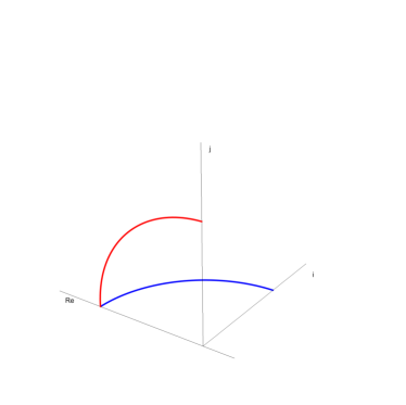
is not continuous at (the left and right limits are different). Therefore cannot be lifted to .
Figure 1. The arc
(b)
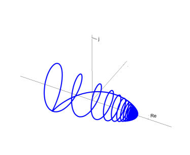
Consider now the loop defined by
where are the usual orthogonal imaginary units (see Figure 2). Notice that the imaginary part of is continuous at all points of the interval (including ). Nevertheless, for near to , we have that the function
has no limit for approaching . Therefore cannot be lifted to .
(c)
Notice that in both the preceding cases, the paths and can be lifted to , since their images are included in (see Proposition 4.5).
Figure 2. The path (negative rocket) of the Example 4.6 (b) is drawn on the left: it cannot be lifted to . Its reflection on the right (positive rocket) can be lifted to .
It is useful to point out that the existence of a lift of a path to
is equivalent to the existence of a continuous function
, such that
As noticed in Remark 2.1, the function will be decomposed, where possible, with obvious notation, as
where and . The existence of
implies that we can assign to each
a complex plane which contains the
point and hence determines the argument up to a multiple of
Complex slices are naturally parameterized by the elements of , the real projective space of dimension .
The projection is the classical universal covering map and, as customary, for , the symbol denotes the equivalence
class whose representatives are the opposite (conjugate) imaginary
units Each element uniquely defines the
complex slice . A
continuous imaginary unit function naturally defines a continuous function when we set
Definition 4.7.
.
Let and let be a path.
A path such that for every is called a companion of the path .
If a companion of the path exists, then is called a path with a companion and the pair is called a path with companion .
If the path has a unique companion , then both and the pair are called a tame path.
Proposition 4.8.
Let be a path with companion . If are the two lifts of of , then there exist continuous functions such that, for all ,
These last expressions are called canonical forms of .
Proof.
Since and are both continuous, then and are continuous as well on .
∎
It is easy to see that all paths lying entirely in a complex slice have a companion. Notice as well that a path may have more than one companion: this happens for example when the path is such that ; in this case, for an arbitrary path , the induced path is a companion of ; consequently is not tame. For a similar reason, a path which maps a closed sub-interval of to a real number has more than one companion, and hence is not tame.
Remark 4.9.
There exist paths in which can be lifted to , but have no companion. Indeed, set
where is the path defined in Example 4.6 (a). The path is the symmetric image of the path with respect to the plane of purely imaginary quaternions (see figure 1) and, as pointed out in Example 4.6 (c), it can be lifted to . Obviously has no companion: the continuity of a companion cannot hold at .
The following definition will play a central role in the sequel.
Definition 4.10.
Let
be a path with a companion , let be the two h (continuous) lifts of to and let
be the canonical forms of .
The paths defined by
are called the (two conjugated) shadows associated with the pair . If the path is tame, then the paths and are simply called the (two) shadows associated with the path .
Remark 4.11.
The two shadows associated with the pair (, ) are conjugate paths.
Paths with a companion are of interest because they can all be lifted to .
Proposition 4.12.
Let be a path with companion . Then there exist
•
a path with , for all ,
•
a path ,
such that, after setting , the path
is a lift of to with , called a -lift of .
If, as in Definition 3.5, for every we set and , then the path
is a -lift of to with .
Proof.
There exist exactly two continuous lifts
of to the universal covering of . Correspondingly, there exist two shadows associated with . Exchange and if necessary, so that is such that .
As a complex path, has a well defined argument such that . Set . Then the chosen paths and have the properties required in the statement.
The rest of the proof is straightforward.
∎
The lifts and (for ) appearing in the last Proposition are not unique, when and are real.
At this point, Proposition 4.2 implies directly the existence of all branches of the logarithm, along all paths in having a companion.
Corollary 4.13.
Let be a path with companion . For every , let
be a -lift of to with . Then, the map defined on the interval by
is a continuation of the hypercomplex logarithm along with initial point . This map is called a -th branch of the hypercomplex logarithm along with initial point .
Proof.
The proof is a straightforward consequence of Proposition 4.12 and Proposition 4.2.
∎
We will now turn our attention to the case of loops of .
Definition 4.14.
Let and let be a path with a companion .
If both and are closed, then the path is called a loop with companion , and the pair is called a loop with companion.
The loop with companion is called untwisted if is homotopic to a constant in ; if instead is not homotopic to a constant, then is said to be twisted.
In the most relevant case in which is tame, we can specialize the definition as follows.
Definition 4.15.
Let and let be a tame path with companion .
If both and are closed, then is called a tame loop (with companion ), and the pair is called a tame loop.
The tame loop is called untwisted if is homotopic to a constant in ; if instead is not homotopic to a constant, then is said to be twisted.
Remark 4.16.
For any fixed , let be a path lying in the complex slice . The path has always a particularly simple companion, namely constantly equal to . Moreover, the two different lifts of to are both constantly equal to or , respectively. As a consequence, if the given path is closed and tame, it is a tame loop and is untwisted.
A twisted loop necessarily intersects the real axis. Indeed the following result holds.
Proposition 4.17.
Let be a loop which misses the real axis. Then is a tame loop and is untwisted.
Proof.
By Proposition 4.5, the loop can be lifted to a path with . Let us consider the map . By the hypothesis, there exists such that the map is never vanishing and hence has constant sign. Now, since is closed, we have that
Since and have the same sign and both belong to the interval , we obtain
and hence
Therefore the path is a loop, and hence the unique companion is a loop, homotopic to a constant. As a consequence the path is an untwisted, tame loop.
∎
4.1. Winding number for untwisted loops with companion in
It is well known that the definition of winding number for a loop (with respect to a point) is not natural in when is greater than . Nevertheless, in our setting, we can start by giving a definition of winding number that has full meaning for loops with companion that are untwisted and lie in .
The following result opens a way to this definition of winding number.
Proposition 4.18.
A loop , with companion is untwisted if, and only if, for any chosen non real initial point of , both shadows associated with are loops.
Proof.
Let ,
be one of the shadows associated with .
If the loop is untwisted, then any lift of the companion of is a loop, and hence it has coinciding endpoints. Therefore, the path
being a loop, the continuous function is such that . Hence the associated shadow
is closed.
On the other hand, suppose the associated shadow ,
,
is a loop and assume that Since the path
is a loop by assumption, we obtain and so the lift of is a loop. In conclusion, is untwisted.
∎
We are now ready to use the well established definition of winding number for complex loops in to define the winding number in the case of untwisted loops with companion in .
Definition 4.19.
Let the loop with companion be untwisted.
The winding number (with respect to zero) of the loop , denoted , is defined as the absolute value of the winding number (with respect to zero), , of a shadow associated with :
In the case in which the loop is tame, there is one and only one companion of , and hence we can simply denote the winding number of by
.
Of course, we need to show that the given definition of winding number of an untwisted loop with companion does not depend on the choice of the shadow associated with . Indeed, the two shadows associated with are conjugate loops: as a consequence, their winding numbers are opposite. Therefore, Definition 4.19 is consistent.
One of the important features of the classical winding number (with
respect to zero) of loops of is its invariance with
respect to homotopy between such loops. The winding number of an
untwisted loop with companion (in ) just defined
cannot be invariant with respect to standard homotopy in :
all such loops are homotopic to a constant loop since
is simply connected, and a constant loop has
vanishing winding number.
A special notion of homotopy comes into the scenery in our setting. The next definition is useful to define such a notion.
Definition 4.20.
Let and let be a continuous map.
A continuous map such that for every is called a companion of the map .
If a companion of the map exists, then is called a continuous map with companion , and is called a continuous map with companion.
If the map has a unique companion , then it is called a tame map.
Proposition 4.21.
Let be a continuous map with companion . If are the two lifts of , then there exist continuous functions such that, for all ,
These last expressions are called canonical forms of .
As announced, the idea is now to define a special type of homotopy between paths, each having a companion and sharing the same endpoints. As customary, also in this paper homotopy between paths will always be meant with fixed endpoints.
Definition 4.22.
Let be two paths with the same endpoints
and . Let and be companions of and respectively.
If there exists a continuous map with companion such that:
(1)
and , for all ;
(2)
and , for all ;
(3)
and , for all ;
then we will say that are companion homotopic (or c-homotopic) and that is a c-homotopy between and .
Let be two paths with the same endpoints. If there exist a companion
of and a companion of such
that are c-homotopic, then we say that
and are weakly c-homotopic.
The following simple result will be helpful in the sequel.
Proposition 4.23.
Let the continuous map with companion be a c-homotopy between and .
Then:
(i)
the map is a homotopy between and ;
(ii)
the homotopy can be lifted to a homotopy between a lift of and a lift of in such a way that the canonical form of
(4.3)
is a homotopy between the canonical forms
and
of and , respectively;
(iii)
the shadows
of and , respectively, are homotopic in .
Proof.
The proofs of (i) and (ii) are a straightforward consequence of Definition 4.22 and of what is stated in Propositions 4.8 and 4.21. Let us prove (iii). To this aim, consider the canonical form of that appears in (4.3) and the following continuous maps, for :
We will prove that is a homotopy between the two given shadows of and . Indeed, using directly formula (4.3) for the canonical form of , it is easy to check that on ,
The proof is now complete.
∎
Example 4.24.
To better illustrate the major difference between complex and quaternionic cases, consider the complex curve, defined by
As a complex curve, i.e. with the constant companion the curve has winding number and coincides with its own shadow.
As a quaternionic curve, has a large family of companions ; for example one can consider-
and , where is an arbitrary continuous
curve with and
Correspondingly, the shadow of is
and so the winding number of is The pairs and are not c-homotopic.
The notion of c-homotopy is particularly useful in this setting, because of the following result.
Proposition 4.25.
Let be two paths with companions and with the same endpoints and . Then the following statements are equivalent :
(1)
are c-homotopic;
(2)
and are homotopic in , and, in addition, for each of the shadows of there is a shadow of so that these two shadows are homotopic in .
Proof.
Suppose first that (2) holds. Then there exist:
•
a homotopy between and ;
•
a lift of , i.e. a homotopy between a lift of and a lift of ;
•
a homotopy between a shadow of and a shadow of (its “conjugate” being a homotopy between the corresponding conjugate shadows).
In this situation, the map defined by
is a homotopy between and . Indeed, is obviously continuous, and such that, for all and all ,
Moreover, the continuous map defines, by construction, a companion of given by
for all . As a consequence, is a c-homotopy between .
Let us now suppose that (1) holds, i.e. that and are c-homotopic.
In this case and are homotopic by definition, and the rest of the assertion follows from Proposition 4.23.
∎
Proposition 4.26.
Let be a loop with companion . Then is untwisted if, and only if, it is c-homotopic to one of its (closed and conjugate) shadows in .
Proof.
If is untwisted, then any lift of the companion with initial point is homotopic in to the constant loop , and therefore the loop is c-homotopic to its (closed) shadow in (see Proposition 4.18). On the other hand, if the loop with companion is c-homotopic to its shadow, then the lift of its companion with initial point has to be homotopic in to the constant loop . As a consequence the loop is untwisted by definition.
∎
The notion of c-homotopy is suitable to comply with the meaning of the winding number of loops in the setting of .
In this panorama, all untwisted tame loops play a special role: any such a loop has an “intrinsically defined” winding number that depends only on its geometric properties. Indeed, we can state the following result.
Theorem 4.27.
Let be two untwisted, tame loops. Then and are c-homotopic if, and only if, .
Proof.
By Proposition 4.25, and are c-homotopic if, and only if, the unique companions and are homotopic and a shadow of is homotopic to a shadow of , in .
According to Definition 4.19, the winding number of (or ) is defined as the absolute value of the winding number of one of the two (closed) shadows of (or ). Therefore the proof is a straightforward consequence of the properties of the fundamental group , where the class of each loop is determined by its winding number (with respect to zero).
∎
The given definition of winding number, which has particularly transparent geometrical meanings, cannot be adopted as it is in the twisted case, due to the two following results.
Proposition 4.28.
Let be a loop with a companion . Then is twisted if, and only if, for any chosen non real initial point of , any shadow associated with has conjugate endpoints.
Proof.
Let ,
be one of the shadows associated with .
If the loop is twisted, then the lift is not closed, and hence it has opposite endpoints. Therefore, the path
being closed, the continuous function is such that . Hence the associated shadow
has conjugate endpoints.
On the other hand, suppose the associated shadow ,
,
has conjugate nonreal endpoints. Then and, the path
being closed by assumption, we obtain and so the lift of is not closed. In conclusion, is twisted.
∎
Corollary 4.29.
Let be a loop with companion . Then the two shadows associated with are closed if, and only if, the endpoints of are real.
Proof.
The proof follows immediately from Proposition 4.28.
∎
We might be encouraged to think that, in the case of a loop with companion which is twisted, we should first parameterise the loop in such a way that it has real endpoints (see Proposition 4.17), and then use Definition 4.19. Indeed, this approach gives a weird result, if tested, for instance, in the case of the twisted, tame loop presented in the next example.
Example 4.30.
Consider the loop in the hyperplane
of generated by the orthogonal units . The path consists of
several arcs: the arc of parabola
the segments from to , from to
and from to the halfcircle and the quarter of circle Let the orientation be such that it
coincides with the positive orientation of the halfcircle part in
the plane containing . The path intersects the real axis at points and
Figure 3. From left to right: (a) the path and two of its shadows (b), (c) aaaaaaaaaaaaaaaaa
In the previous example, the proposed winding number of the twisted,
tame loop would be if the loop is parameterised with
real endpoints equal to (see Figure 3 (b)). On the other hand, the same
loop
parameterised with endpoints equal to would have
winding number (see Figure 3 (c)). What we just
illustrated clarifies that a notion of winding number for twisted,
tame loops in (if it exists) has to be given by
following a different approach.
In the spirit of the above example and Proposition
4.28 the definition of the winding number for a
closed tame twisted loop
cannot be given by considering
the change of the argument since
this depends on the choice of the initial point.
Assume that is a twisted loop in which
intersects both the positive and the negative real axis;
let , be one of the shadows
associated with . Let be the
corresponding argument and choose the initial argument so that
The set is an interval contained in
Because the
loop
is twisted, the argument at is
and hence
and
is not an integer multiple of unless Even if we set the initial point to be real, so that the
change of argument is the number can have more than one
value as shown in the following example.
Example 4.31.
Let be the positively oriented unit circle with initial
point and companion and define . Choose the lift of the
companion of so that and Let
denote
the loop composed first of copies of
followed by a copy of If
the initial point is assumed to be
the point on the first copy of , then the change of
the argument is If the initial point is the point on
the second copy of ,
then the copies of
before give the
winding number , but then the curve reverses the
orientation so the last copy of has negative orientation
with respect to the unit hence the winding number is
Starting at on the third copy
of ,
would therefore result in the
winding number and so forth.
A few words seem now appropriate, to present a suggestive geometrical explanation of the reason why the notion of winding number as given in the case of untwisted loops does not work for the case of twisted loops. Indeed, consider an untwisted loop
If we regard all points as distinct points except the endpoints, such a has values in the surface ; since is untwisted, then is a loop, and hence it is homotopic to the constant loop . As a consequence, the surface is homeomorphic to a twodimensional cylinder. Therefore there is a notion of being a point of this surface lying on one side or the other of the “real axis” formed by the points , and hence a notion of winding number with respect to the origin becomes possible: the situation reduces, naively speaking, to a planar one. If instead is twisted, then the path has antipodal endpoints, and the surface turns out to be homeomorphic to a Moebius strip. In this last situation, the lack of orientability seems to exclude the possibility of defining coherently a winding number for the loop .
5. Obstructions to the existence of lifts of a path
In this section we present sufficient conditions for a path to have a lift, a companion and to be tame.
As already mentioned, if the path misses the real axis, then the lift to always exists. On
the other hand, if , then,
necessarily either and we have
the lifts of the form , or
and then we have the lifts of the
form for any From
now on assume that is not entirely contained in the
real axis but it intersects it.
Definition 5.1.
For a path we define the set to be the
obstruction set (for the lift of ) and its points as obstruction parameters.
It is clear that the necessary assumption for a lift of to
to exist is the requirement that has a
lift on a neighbourhood of every parameter in particular, for
each It turns out that the existence of local lifts does
not necessarily imply the existence of a global lift; recall that
complex curves avoiding always have local and global lifts.
In what follows, we start establishing the conditions on the
behaviour of locally near its obstruction parameters in order to guarantee the existence first of local lifts and local companions and then of a global lift and a global companion.
As these conditions depend on the structure of the obstruction set, we start by considering paths with a finite obstruction set.
Definition 5.2.
Let the path be such that
Consider the limits
(5.4)
Let Then
1)
is tame at if both limits
are either equal or opposite. In particular,
if these limits are opposite, then the parameter is called a flip, whereas if they are the same it is called a bounce;
2)
is semi-tame at if it is not tame at but both limits in (5.4) exist;
3)
is not tame at if at least one
of the limits in (5.4) does not exist.
If (resp. ) then the path is tame at from the right (left)
if the right (left) limit in (5.4) exists and not tame in all other cases.
If, in addition, the path is closed, we adapt the definition of tameness at the endpoints in the natural way. In particular,
is semi-tame at if it is tame at from the right and at from the left. If the limits are the same, then is called a bounce and if they are opposite it is called a flip. In all other cases is not tame at
Remark 5.3.
A path in the Example 4.6 (b) does not have the limit (5.4) at
Remark 5.4.
The definition of tameness of at parameters means precisely that the projectivized imaginary unit function defined on
has a continuous extension to .
The proposition below gives a motivation for the previous definitions.
Proposition 5.5.
Let be a path with finite obstruction set
Then is tame if and only if it is tame at each
If is a loop, then it is a tame loop if and only if it is tame at each
Proof.
By assumption, the projectivized imaginary unit function defined on
has a continuous extension to
∎
If is a tame loop, the lift to exists by Proposition 4.12.
However, we want to present also a constructive proof, because we will
use the same techniques to obtain lifts of non tame paths and to explain the definition of winding number through local data on the obstruction set.
Without loss of generality we assume that Consider the intervals and denote the
restrictions of on by The existence
of limits (5.4) provides, for any
continuous extensions of all functions
to the endpoints of
Choose an arbitrary Setting and we define continuous functions and on
We set and define the lift
Consider the endpoint If it is a flip, then we
define
If it is a bounce then we set
By setting and we
extend the functions and
continuously to We extend the above functions to by repeating this process.
Proposition 5.6.
A tame loop with has an even number of flips if and only if is untwisted.
Proof.
Assume that the loop does not have flips. Then equals
for some
and so it is obviously a loop.
For the case of a loop with flips, we assume, without loss of generality, that
so we have started with the principal branch and moreover, we also assume that the
parameterization is such that
As in the previous proof, all the functions
have continuous extensions to
the endpoints of
If is a bounce, then the imaginary unit at is
the same as the one at , i.e. The even
number of flips ensures that the sign of the imaginary unit at the
endpoint remains the same with respect to the one at the principal
branch.
If the initial point is a flip, then the imaginary unit function at
endpoint has the opposite sign with respect to the one at the initial
point, and to end up with
the same sign there must be an odd number of additional flips
following the first one to ensure that the sign of the unit at the
endpoint remains the same with respect to the one at the principal
branch.
∎
The proofs of Propositions 5.5 and 5.6 show that once
the lift near the initial point is chosen, only the flips are relevant
for the determination of the lift near the endpoint; bounces can be
discarded. This enables us to calculate the change of argument and the
winding number out of local data at the intersections of with
the real axis. To determine the change of the argument we introduce a
notion of signature.
Definition 5.7.
Let be a given path with , with points of all tame. Let be those parameters
in which are flips. The signature is defined by
If there are no flips, then we define
The connection between the signature and the change of argument is described in the following
Proposition 5.8.
Let be a tame path with
with all the parameters tame. Assume that a lift
of in
exists
and equals
for some .
Then the lift of is given by
Remark 5.9.
If , then a lift of on can be extended continuously to if and only if is tame from the left.
Corollary 5.10.
Let be as in Proposition 5.8 and let Then is even if and only if is tame and untwisted.
If this is the case, then
Proof of Proposition 5.8. Assume that so and let the sequence of signs of flips be alternating starting with i.e.
Then increases when the path crosses the real axis,
so increases by at each flip (because the sign of the flip changes); altogether, this occurs
times. This coincides with winding around
the origin of the shadow in the positive
direction. If the sequence of signs starts with then
decreases when the path crosses the positive real axis and
this results in the translation of the interval by
To prove the general assertion it suffices to show what happens if the sequence is not alternating at one position.
Assume that we insert in the alternating sequence the
integer in the second position, so the sequence is no longer
alternating: This means that we have started from
the upper half-plane, crossed the negative real axis, then the
positive real axis with the arguments in Then we have
crossed the positive real axis again, hence the choice of argument at
this intersection must be Because the point is a flip, this
means that the argument decreases and keeps decreasing till the end.
This is faithfully reflected in the sequence because it equals and so the sum
multiplied by corresponds with the total translation of the
initial interval for the Arg.
Similarly, if we insert on the second position, this means that
we have crossed the negative real axis and we have the argument in
but then we have returned to the negative real axis and
in order to have the argument continuous, at the second crossing the
argument must be chosen and because we have a flip, the argument
decreases and keeps decreasing till the
end. The corresponding sequence now equals
and
The proof for even is the same. If is odd, this coincides with considering the conjugate shadow and hence reversed
orientation compared, to even, so the signature has to be multiplied by to get the total translation of the initial interval for the Arg.
In practice this means that once the sequence of -s is given,
we start by cancelling the pairs of the same numbers until we end
up with an alternating sequence. The number of elements multiplied by
minus the first element is the signature.
If the path is closed,
i.e. , then we identify points and of and
consider the parameterization as so there is no distinguished initial point. Therefore, in this
case we require that for each there exists a neighbourhood
of of in such that the lift of exists on
Definition 5.11.
Let be a continuous loop. Then a continuous function
is a lift of if
the following diagram commutes:
Remark 5.12.
A loop with companion always has a (not necessarily closed) lift in the sense of Definition 5.11. The loop presented in Figure 4 does not have a lift in the sense of Definition 5.11.
The curve is defined by for
and for However, starting from any
point with and using the principal
branch one can obtain the local lift of and prolong it to the
interval
Figure 4. A loop without a lift in the sense of Definition 5.11.
Corollary 5.13.
Let be a continuous loop with
nonempty and assume it is not tame at least at one of the obstruction parameters.
Let are all the
obstruction parameters where is not tame and assume, moreover, that Then a lift of in exists if and only if
for each
If it exists, the lift is a loop.
Proof.
Because is not tame at we can only choose either or
and lift the curve in a neighborhood of the point to using the principal branch of the logarithm.
Assume that we have chosen . Then on for some small we may only have
hence the signature can be either or in order to be able
to extend the lift to If we have then,
since we have to end up with near the
condition is hence
∎
When we do not have additional information about the
set ,
we must assume that the continuous lift of
exists on a neighbourhood of . This means that the path has a companion, since
the restriction of the function to is not vanishing.
Recall that, on a neighbourhood of
, the principal branch of the logarithm
is well-defined
and hence a lift of always exists. This does not imply that a global lift exists.
We now proceed with the detailed description of the possible situations
when has a companion on a neighborhood of real points and omit the (trivial) case .
Proposition 5.14.
Let be a path. Then has a companion if and only if it has a companion on a neighbourhood of the obstruction set. The same holds for a loop with .
In the sequel we explain how to extend the notion of signature to paths with infinite obstruction set. Since is compact, there are only finitely many connected components
of with endpoints of opposite
sign.
Definition 5.15.
Let be all the connected components of satisfying and , . We call the
components the big arcs and the subdivision , the induced
subdivision. The intervals are called obstruction intervals. If is closed, then we identify
and and define also as
the obstruction interval.
Because misses either the positive or the
negative real axis, we define the sign of the obstruction interval as follows.
Definition 5.16.
If
then ;
otherwise, if then
Extend the domains of definition of each to its
endpoints and let
be the imaginary units of at its endpoints, if the
limits exist.
Definition 5.17.
Let be a path with companion with lifts Let
be the induced subdivision and the big arcs with limits
and .
The interval is a bounce with respect to if (or )
satisfies and a
a flip with respect to if (or ) satisfies
Remark 5.18.
If has a companion and contains an open set then always has a companion that makes it a bounce and a companion that makes it a flip. If the interval
reduces to a point, then the definition of tameness for intervals
coincides with the definition of
tameness for points.
We can now extend the definition of signature also to this general case.
Definition 5.19.
Let be a path with the induced subdivision and a companion
Let be the indices for which the intervals
are flips. The signature with respect to the companion is defined as
If is a loop, then we define the circular
signature with respect to to be
If there are no flips, then we define
The following are straightforward generalizations of Proposition 5.8 and Corollary 5.13
Proposition 5.20.
Let is a path with the companion and the induced subdivision
Assume that a lift of in
is given by on for some
The lift on is given by
To define the winding number for a closed curve we have to take into account also the last interval and hence consider the closed signature.
Corollary 5.21.
Let be a loop and even. Then
Corollary 5.22.
Let be a loop with the induced subdivision
Let be the indices for which restricted to the neighbourhoods of the intervals
does not have a companion and assume has a companion on a neighbourhood of the closure of
Then a lift of in exists if and only if
for each
If it exists, the lift is a loop.
References
[AdF]A. Altavilla, C. de Fabritiis, *-exponential of slice regular functions,
Proc. Amer. Math. Soc. 147, 1173-1188, 2019.
[AdF1]A. Altavilla, C. de Fabritiis, *-logarithm for slice regular functions, to appear in Rendiconti Lincei - Matematica e Applicazioni arxiv.org/pdf/2106.04227.pdf
[GGS]G. Gentili, A. Gori, G. Sarfatti, A direct
approach to quaternionic manifolds, Math. Nachr., 290 (2017),
321–331. https://doi.org/10.1002/mana.201500489
[GPV]G. Gentili, J. Prezelj, F. Vlacci,
Slice conformality and Riemann manifolds on quaternions and octonions,
Math. Z. 302, (2022), 971–994
[GPV1]G. Gentili, J. Prezelj, F. Vlacci, On a definition of logarithm of quaternionic functions, to appear in Journal of Non Commutative Geometry https://arxiv.org/abs/2108.08595v1
[GSS]G. Gentili, C. Stoppato, D. Struppa, Regular functions of a quaternionic variable, Springer Monographs
in Mathematics, Springer, Heidelberg, 2013.
[GS]G. Gentili, D. Struppa, A new theory of regular functions of a quaternionic variable, Adv. Math., 216, 279–301, 2007.
[GV]G. Gentili, I. Vignozzi, The Weierstrass
factorization theorem for slice regular functions over the
quaternions. Ann. Glob. Anal. Geom. 40 (2011),
435–466. https://doi.org/10.1007/s10455-011-9266-0
[GP]R. Ghiloni, A. Perotti, Slice regular
functions of several Clifford variables, Proceedings of ICNPAA 2012
- Workshop “Clifford algebras, Clifford analysis and their
applications”, AIP Conf. Proc. 1493, pp. 734-738, 2012