Physics-Informed Neural Networks for Parametric Compressible Euler Equations

Abstract

The numerical approximation of solutions to the compressible Euler and Navier-Stokes equations is a crucial but challenging task with relevance in various fields of science and engineering. Recently, methods from deep learning have been successfully employed for solving partial differential equations by incorporating the equations into a loss function that is minimized during the training of a neural network. This approach yields a so-called physics-informed neural network. It is not based upon classical discretizations, such as finite-volume or finite-element schemes, and can even address parametric problems in a straightforward manner. This has raised the question, whether physics-informed neural networks may be a viable alternative to conventional methods for computational fluid dynamics. In this article we introduce an adaptive artificial viscosity reduction procedure for physics-informed neural networks enabling approximate parametric solutions for forward problems governed by the stationary two-dimensional Euler equations in sub- and supersonic conditions. To the best of our knowledge, this is the first time that the concept of artificial viscosity in physics-informed neural networks is successfully applied to a complex system of conservation laws in more than one dimension. Moreover, we highlight the unique ability of this method to solve forward problems in a continuous parameter space. The presented methodology takes the next step of bringing physics-informed neural networks closer towards realistic compressible flow applications.

[inst1]organization=German Aerospace Center - Institute for Aerodynamics and Flow Technology
Center for Computer Applications in Aerospace Science and Engineering, addressline=Lilienthalplatz 7, city=Braunschweig, postcode=38108, country=Germany

Nomenclature

List of Symbols

$\bm{u}$	general solution to boundary value problem
$\bm{\hat{u}}$	neural network output vector
$\Omega$	spatial domain
$\mathcal{D}$	general differential operator
$\mathcal{B}$	boundary condition
$\mathcal{I}$	initial condition
$\bm{x}$	vector of euclidean coordinates
$t$	time
$T$	upper limit of time
$\rho$	density
$x$	first euclidean coordinate
$y$	second euclidean coordinate
$u$	velocity in x-direction
$v$	velocity in y-direction
$E$	total specific energy
$H$	enthalpy
$p$	pressure
$\bm{q}$	velocity vector
$\bm{W}$	vector of conserved variables
$\bm{W}_{\infty}$	vector of conserved variables at far-field
$\bm{F}_{x}$	flux vector in x direction
$\bm{F}_{y}$	flux vector in y direction
$\kappa$	ratio of specific heats
$\tau$	general parameter of PDE or boundary conditions
$\tau_{\mathrm{min}},\tau_{\mathrm{max}}$	lower and upper bound of $\tau$
$N$	number of points for residual evaluation
$N_{\infty}$	number of points for Dirichlet/far-field boundary condition
$N_{\mathrm{ob}}$	number of points on obstacle surface for wall boundary condition
$\mathcal{L}$	total loss functional
$\mathcal{L_{\mathrm{Res}}}$	residual loss term
$\mathcal{L_{\mathrm{I}}}$	initial loss term
$\mathcal{L_{\mathrm{B}}}$	boundary loss term
$\mathcal{L_{\mathrm{\nu}}}$	viscosity penalty loss term

$M_{\infty}$	Mach number at far field
$M$	local Mach number
$\eta$	artificial viscosity
$\nu$	artificial viscosity factor
$\tilde{\nu}$	prescribed artificial viscosity factor
$M_{\mathrm{red}}$	number of reduction epochs
$k$	order of reduction function
$\alpha$	weighting factor for initial condition loss
$\beta$	weighting factor for boundary condition loss
$\gamma$	weighting factor for viscosity penalty loss
$a$	semi-major axis of ellipse
$b$	semi-minor axis of ellipse
$e$	eccentricity of ellipse
$lr$	learning rate
$\theta$	deflection angle for oblique shock
$\delta$	angle between shock and wall
$C_{p}$	coefficient of pressure
$r$	radius of cylinder
$N_{\mathrm{batch}}$	number of point per mini-batch
$\omega^{k}$	trainable parameter in adaptive activation layer $k$

Abbreviations

PINN	physics-informed neural network
LBFGS	Limited-memory Broyden-Fletcher-Goldfarb-Shanno algorithm
ADAM	adaptive momentum estimation optimization algorithm
PDE	partial differential equation
AD	automatic differentiation
CFD	computation fluid dynamics

1 Introduction

The motion of compressible fluids gives rise to nonlinear partial differential equations (PDEs) such as the Euler and Navier-Stokes equations. The numerical solution of these equations is for example essential for the development of future aircraft configurations. State of the art solvers typically rely on finite volume or finite element algorithms [1, 2, 3, 4]. These algorithms have been developed and refined for decades and they are in regular use for industrial problems such as aircraft design. These classical algorithms discretize the domain and thus require the construction of carefully crafted computational grids, so-called meshes. Superficially speaking, a finer mesh will result in a more accurate result but will also increase the computational cost needed. Despite a non-negligible progress in efficiency in recent years, long term prospects for further acceleration of these codes seem limited. Especially, transferring these methods to potentially advantageous hardware like graphic processing units has shown to be challenging. Besides, classical algorithms solve a problem for one specific instance of boundary conditions and/or initial conditions. Therefore, for certain tasks, such as design optimization, multiple evaluations of the solver are necessary. The cumulative computational effort of multiple solver evaluations can be significant and is therefore a possibly limiting factor for the usage for commercially relevant problems.

Our interest is to investigate numerical methods which have the potential to be applied on future hardware promising an acceleration of orders of magnitude. In particular, some initial works indicate that one may be able to transfer deep learning based approaches to quantum computers [5], even though the potential for acceleration on this hardware is currently still unclear. In addition, to successfully implement such an approach, it is necessary to explore the methodological basis that is required for successful algorithmic implementation. With the rising popularity of machine learning methods and especially deep neural networks, alternative approaches for the solution of differential equations, based on methods from this rapidly advancing field have become a popular alternative to classical solvers

One of these techniques are Physics-Informed Neural Networks (PINNs). The fundamental idea of PINNs is to use a neural network as a parametric ansatz function for the approximation of the PDE solution and to optimize the networks parameters by minimizing a loss functional which directly incorporates the differential equations as well as the initial and boundary conditions. During the training of the network, the loss functional is evaluated at random points inside of the domain. PINNs are fundamentally different to classical algorithms because they do not rely on a spatial or temporal discretization in a classical sense. Instead a continuous parametric ansatz-function (a neural network) is evaluated and optimized at (oftentimes randomly distributed) points in the domain. Hence, the task of mesh-generation is replaced by the task to find a point distribution in space and time and an appropriate network dimension (i.e. number and width of layers) which, when combined, result in a fast convergence and satisfactory final accuracy.

Compared to classical methods, PINNs can directly tackle parametric problems. A single network can be trained in a continuous parameter space and yield approximate solutions for a whole range of parameter combinations of interest. This ability may have implications for aforementioned use cases like design optimization.

Similar approaches for approximating PDE solutions via neural networks have been proposed decades ago in works of Lagaris et al. [6] and Dissanayake et al. [7]. Even though the idea seems natural due to the ability of universal function approximation of neural networks [8], the method has only recently gained popularity. Nowadays, the networks can be trained more efficiently due to the availability of high performance graphics cards. Moreover, the implementation of such algorithms has become straightforward with software libraries for deep learning, such as Tensorflow [9] and PyTorch [10]. The term PINN has been introduced by Raissi et al. [11] who demonstrated the use of this approach on a number of nonlinear PDEs for forward and inverse problems. Subsequently, PINNs have shown to be applicable for solving stochastic PDEs [12], inverse problems [13] and parametric problems [14]. Various alterations of the vanilla PINN formulation have been proposed and improvements for the implementation of boundary conditions [15, 16, 17], training facilitation [18, 19] and training point selection [20, 21] have been developed. For high frequency problems and large domains, the limited expressibility and the frequency bias of neural networks may limit the applicability of PINNs. Therefore, different domain decomposition approaches have been proposed, which divide the domain into smaller subdomains and use separate networks to approximate the solution in each subdomain. In particular Jagtap et al. have proposed the conservative PINN [22] and extended PINN [23] approaches which use disjoint subdomains and predefined interface conditions to enforce continuities at the common interfaces of subdomains. Each network for the respective subdomain is trained with a separate loss function and the training procedures can be parallelized efficiently [24]. On the other hand, soft domain composition approaches such as augmented PINN [25] and finite basis PINNs [26] use overlapping subdomains and smooth gating or blending functions which locally determine the contribution of each network to a particular point in the domain. The final prediction is the sum of all sub-network predictions, weighted with the window/gating functions. Augmented PINNs use additional trainable gating networks while finite basis PINNs use fixed analytical window functions. Among many other domains, the flow simulation community has readily adapted PINNs for various cases such as blood flow [16, 27], turbulent convection [28] and aerodynamics of airfoils [29]. An important property of PINNs is the fact they allow for a straightforward integration of additional available data from various sources such as experiments or higher fidelity simulations into the training process. Raissi et al. [30] demonstrate how noisy concentration data of a passive flow agent can compensate for incomplete boundary conditions. Even for compressible flows, there has been some success to employ PINNs for simple forward and especially inverse problems which exhibit discontinuities [31, 22, 32]. Again, the introduction of additional solution data into the loss is used to compensate for incomplete boundary conditions. For a more extensive overview on the usage of PINNs for fluid dynamics the interested reader is referred to [33].

Fuks and Tchelepi [34] have identified the need for additional dissipation when solving one dimensional hyperbolic conservation laws with PINNs once shocks are present. They pointed out the similarity to classical methods, which use artificial dissipation to approximately solve conservation laws. Recently, Coutinho et al. [35] have proposed multiple methods to locally or globally choose artificial viscosity values. They demonstrate the efficacy of their method on one dimensional transient PDEs. Here we take this idea to more complex problems by solving the stationary compressible Euler equations in two spatial dimensions. The compressible Euler equations are a system of conservation laws with four dependent variables (typically density, the velocity components and the energy) that describe the behavior of inviscid compressible fluids. We also observe that additional dissipative terms are able to facilitate convergence which is the case for supersonic but also for subsonic problems without shocks as shown in A. To avoid highly dissipative solutions, we introduce two novel ideas. On the one hand we predict the locally necessary dissipation strength by letting the network predict the local viscosity alongside the primitive variables. On the other hand, we use a penalty loss term to control dissipation levels during the training. By initially training with high viscosity and then reducing the dissipation later, we obtain non dissipative solutions while facilitating convergence during training. We do, however, not only solve these equations for one instance of boundary conditions, but rather use the ability of PINNs to approximate parametric solutions, essentially extending the dimension of the problems by one or two parameter dimensions. We choose to restrict this analysis to classical forward problems, meaning that no additional data is incorporated into the loss function, besides the information that is available in the form of fully provided boundary conditions. So far, the investigation PINNs for complex problems governed by the Euler equations has oftentimes been restricted to inverse problems where some form of data of the solution is already provided [31, 32]. While the ability of incorporating this data is clearly an advantage and possibly one of the most important use cases of PINNs, we believe that a solid understanding of the forward problem is necessary for reliably tackling more complex problems (e.g. higher dimensional).

In Sec. 2 we give a general introduction to the standard PINN approach for solving (parametric) initial and boundary value problems. In Sec. 2.2 we discuss the application of the approach to the compressible Euler equations and explain how the incorporation of artificial dissipation during the training can facilitate convergence when looking at the aerodynamic problem of calculating the flow around solid obstacles.

In Sec. 3 we solve the subsonic flow around an ellipse with a parametric boundary shape and and variable Mach numbers. In Sec. 4 we solve the supersonic oblique shock problem with variable Mach number. Consider also Sec. A, where non-parametric solutions to the problems are shown and how PINNs struggle to obtain accurate predictions without artificial viscosity. Finally, in Sec. 5 the presented results are evaluated in a more general context and future implications as well as newly arising questions are discussed. The novelties of the paper are twofold. To the best of our knowledge for the first time, we solve parametric problems, governed by the two dimensional compressible Euler equations with PINNs. In addition we introduce a novel adaptive viscosity training procedure which improves prediction accuracy of PINNs on supersonic problems significantly, compared to previously published results. Compared to previous work in [32] we focus exclusively on forward problems. In A, we show that these require additional measures such as artificial viscosity to reliably obtain physically reasonable solutions. This has also been shown for more simple conservation laws in Fuks and Tchelepi [34] and Coutinho et al. [35] confirm the efficacy of artificial viscosity on one-variable conservation laws. Compared to the work on forward problems by Mao et al. [31] we focus on parametric and thus more complex forward problems and obtain better resolution of shocks in the parametric formulation, compared to their non-parametric result (see Fig. 10). For more details, please consider Sec. A. Preliminary results of the presented ideas have been presented at the 8th European Congress on Computational Methods in Applied Sciences and Engineering [36].

Figure 1: Schematic representation of the physics-informed neural network approach for solving the 2D stationary Euler equations. A fully connected neural network predicts the primitive variables $\rho,u,v,E$ and the local viscosity factor $\nu$ at a point $(x,y)$ in the physical domain and for optional parameters of the problem ($\tau_{0},\tau_{1},\dots$). The loss is calculated as the sum of squares of the residual of the PDE, the boundary condition and an additional viscosity penalty term. Partial derivatives of the primitive variables with respect to $x$ or $y$ are required for the loss and can be calculated using automatic differentiation.

2 Methods

2.1 Physics-Informed Neural Networks

Physics-informed neural networks are deep neural networks, which are employed to approximate solutions to differential equations. A general initial-boundary value problem for the unknown function $\bm{u}$ on the spatial domain $\Omega\subset\mathbb{R}^{d}$ and in the time interval $(0,T)\subset\mathbb{R}$ can be defined as:

$$\mathcal{D}(\bm{u}(\bm{x},t),\bm{x},t) =0\;\; (\bm{x},t)\in(\Omega\times(0,T))$$ (1)

$$\mathcal{B}(\bm{u}(\bm{x},t),\bm{x},t) =0\;\; (\bm{x},t)\in(\partial\Omega\times(0,T))$$

$$\mathcal{I}(\bm{u}(\bm{x},0),\bm{x}) =0\;\; \bm{x}\in\Omega,$$

where $\mathcal{D}$ is a general differential operator and $\mathcal{I}$ and $\mathcal{B}$ are the initial and boundary condition, respectively. The operator $\mathcal{D}$ may include multiple nonlinear differential terms of different order. A neural network $\bm{\hat{u}}(\bm{\theta},\bm{x},t)$ is now used to approximate the unknown solution $\bm{\hat{u}}(\bm{\theta},\bm{x},t)\approx\bm{u}(\bm{x},t)$. The vector $\bm{\theta}$ includes neural networks parameters (weights and biases) which have to be adjusted during an optimization/training process to find an accurate approximation of the solution. For this, an objective or loss functional $\mathcal{L}$ is defined. If $\bm{\hat{u}}(\bm{\theta},\bm{x},t)$ is a solution to Eqs. 1, the left hand side of Eqs. (1) vanishes on the entire domain $x\in\Omega$ and for all times $t\in(0,T)$. Therefore, a simple loss functional is

$$\mathcal{L}(\bm{\hat{u}}(\bm{\theta})) = \int_{0}^{T}\int_{\Omega}\mathcal{D}(\bm{\hat{u}}(\bm{\theta},\bm{x},t))^{2}\;\;\mathrm{d}{\bm{x}}\;\mathrm{d}{t}\,+\alpha\int_{\Omega}\mathcal{I}(\bm{\hat{u}}(\bm{\theta},\bm{x},0),\bm{x})^{2}\;\;\mathrm{d}{\bm{x}}\,$$ (2)

$$+ \beta\int_{0}^{T}\int_{\partial\Omega}\mathcal{B}(\bm{\hat{u}}(\bm{\theta},\bm{x},t),\bm{x},t)^{2}\;\;\mathrm{d}{s(\bm{x})}\;\mathrm{d}{t}$$

which is 0 and thus minimal if $\bm{\hat{u}}(\bm{\theta},\bm{x},t)$ is a solution to Eqs. 1. The coefficients $\alpha$ and $\beta$ scale the importance of the boundary and initial loss term with respect to the residual term. Since the network $\bm{\hat{u}}(\bm{\theta},\bm{x},t)$ can only be evaluated at discrete input values, the loss is instead calculated by taking the sum over a representative point distribution inside of the spatial and temporal domain

$$\mathcal{L}(\bm{\hat{u}}(\bm{\theta},\bm{x},t))=\mathcal{L}_{\mathrm{Res}}\;+\;\mathcal{L}_{\mathrm{I}}\;+\;\mathcal{L}_{\mathrm{B}}$$ (3)

$$\mathcal{L}_{\mathrm{Res}}=\frac{1}{N}\sum_{i=1}^{N}\mathcal{D}(\bm{\hat{u}}(\bm{\theta},\bm{x}_{i},t_{i}))^{2}\; \bm{x}_{i}\in\Omega\;;t_{i}\in(0,T)$$

$$\mathcal{L}_{\mathrm{I}}=\alpha\frac{1}{N_{\mathrm{I}}}\sum_{i=1}^{N_{\mathrm{I}}}\mathcal{I}(\bm{\hat{u}}(\bm{\theta},\bm{x}_{i},0))^{2}\; \bm{x}_{i}\in\Omega$$

$$\mathcal{L}_{\mathrm{B}}=\beta\frac{1}{N_{\mathrm{B}}}\sum_{i=1}^{N_{\mathrm{B}}}\mathcal{B}(\bm{\hat{u}}(\bm{\theta},\bm{x}_{i},t_{i}))^{2}\; \bm{x}_{i}\in\partial\Omega\;;t_{i}\in(0,T)$$

where $N_{\mathrm{Res}}$, $N_{\mathrm{I}}$ and $N_{\mathrm{B}}$ are the number of points that evaluate the residual, the initial condition and the boundary condition, respectively. Since for a well defined problem, the bounds of the domain are known, the generation of these training points can be achieved with quasi-random low discrepancy sequences such as Sobol [37] or Halton [38] or with other methods like Latin Hypercube sampling [39] at little additional cost. For a uniform point distribution, the calculation of the loss functional can be interpreted as a Monte-Carlo integration of Eq. (2) where the normalization by the volume has been dropped. As highlighted in various publications [21, 20, 31], a non uniform distribution of training points or an adaptive training point selection, based on the local residual may accelerate training and improve the final accuracy for certain problems.

The partial derivatives in $\mathcal{D}(\bm{\hat{u}}(\bm{\theta},\bm{x}_{i},t_{i}))$ are calculated, using automatic differentiation (AD). The network parameters are then tuned using an iterative optimization algorithm. The most popular algorithms are variants of stochastic gradient descend such as Adam [40]. During the optimization, the gradient of the loss with respect to the network parameters $\nabla_{\bm{\theta}}\mathcal{L}(\bm{\hat{u}}(\bm{\theta},\bm{x}_{i},t_{i}))$ has to be calculated. This can again be achieved, using automatic differentiation and the backpropagation algorithm [41]. As usual for neural networks, the optimization problem is generally non-convex and the optimizer can therefore converge to local minima or regions of vanishing gradients. Furthermore, for partial differential equations such as the compressible Euler equations which may not have a unique solution, a minimum of the loss may not always correspond to a physically reasonable solution.

2.1.1 Adaptive Activation Functions

A general feedforward neural network with $m$ layers and $d_{k}$ neurons per layer can be described as a composition of linear functions and nonlinear activation functions $\sigma$:

$$\hat{u}( \bm{x}^{0}):\mathbb{R}^{d_{0}}\longrightarrow\mathbb{R}^{d_{m}}$$ (4)

$$\hat{u}_{j} \equiv x_{j}^{m}\hskip 28.45274ptj=1,2,\dots,d_{m}$$

$$\bm{x}^{0} =(x^{0}_{1},x^{0}_{2},\dots,x^{0}_{d_{0}})$$

$$x_{j}^{k} =\sigma^{k}\left(\sum^{d_{k-1}}_{i=1}w_{i,j}^{k-1}x_{i}^{k-1}-b_{j}^{k}\right)$$

$$j =1,2,\ldots,d_{k}\;\;\;k=1,2,\ldots,m.$$

A popular choice for the activation function for PINNs is the hyperbolic tangent which has been shown to be a robust choice on a variety of problems [42] compared to other fixed activation functions:

$$\sigma(x)^{k} \equiv\tanh(x)=\dfrac{e^{x}-e^{-x}}{e^{x}+e^{-x}}$$ (5)

$$k =1,2\ldots,m\scalebox{0.75}[1.0]{$-$}1.$$

Note that in the last layer, the identity function $\sigma^{m}(x)=x$ is used. In this work we also make use of the layer-wise locally adaptive hyperbolic tangent activation formulation [43]:

$$\sigma_{\mathrm{adapt}}^{k}(x) \equiv\sigma(n\omega^{k}\cdot x)=\tanh(n\omega^{k}\cdot x)$$ (6)

$$k =1,2\ldots,m\scalebox{0.75}[1.0]{$-$}1,$$

where $n$ is a constant scaling factor and $\omega^{k}$ is an additional trainable parameter per hidden layer that scales the slope of the hyperbolic tangent. Adaptive activation functions have been shown to improve convergence speed [44, 43] and PINN accuracies [42] on various problems, compared to fixed activation functions. The above described version only introduces a single trainable parameter per layer which only marginally increases the computational effort compared to fixed activation functions.

2.1.2 Parametric Problems

One prospect of physics-informed neural networks is the possibility to solve parametric problems. Let $\tau$ be a general parameter of the initial and boundary value problem. A PINN approximation $\bm{\hat{u}}(\bm{\theta},\bm{x},t,{\tau})$ of the unknown solution $u(\bm{x},t,\tau)$ simply receives $\tau$ as an additional input to the neural network alongside $\bm{x}$ and $t$. The parameter adds an additional dimension to the input space and thus the training points. The training points are now sampled in a $d+2$-dimensional domain $(\bm{x},t,\tau)\in\Omega\times(0,T)\times(\tau_{\mathrm{min}},\tau_{\mathrm{max}})$. The parameter $\tau$ can then be incorporated into the calculation of any of the loss terms in Eq. (3). Similarly, this approach can be extended to more than one parameter.

2.2 Approximation of Stationary Compressible Flows with PINNs

The inviscid flow of compressible fluids is governed by the Euler equations which describe the conservation of mass, momentum and energy in a continuous fluid. The two-dimensional Euler equations in their differential conservative form are given by

$$\partialderivative{\bm{W}}{t}+\partialderivative{\bm{F}_{x}}{x}+\partialderivative{\bm{F}_{y}}{y} =0,$$ (7)

$$\bm{W}=\begin{pmatrix}\rho\\ \rho u\\ \rho v\\ \rho E\end{pmatrix},\,\bm{F}_{x}=\begin{pmatrix}\rho u\\ \rho u^{2}+p\\ \rho uv\\ \rho Hu\\ \end{pmatrix},\,\bm{F}_{y} =\begin{pmatrix}\rho v\\ \rho uv\\ \rho v^{2}+p\\ \rho Hv\\ \end{pmatrix}$$

where $\bm{W}$ is the vector of the conservative variables with the density $\rho$, the local fluid velocity $\bm{q}=(u,v)$, and the total specific energy $E$. The total enthalpy $H$ is defined as $H=E+\frac{p}{\rho}$. This system of partial differential equations can be closed by the equations of state of ideal gases, which yield $p=\rho(\kappa-1)(E-\rho\bm{q}^{2}/2)$, with $\kappa$ being the ratio of specific heats ($\kappa=1.4$ for air). The Mach number $M=\|\bm{q}\|_{2}/a$ is the ration between the velocity and the speed of sound $a=\sqrt{\kappa p/\rho}$.

For aerodynamic problems one is oftentimes interested in the steady-state solution. Therefore, the time derivative in Eq. (1) is omitted.

When solving this system of equations with a physics-informed neural network, the network outputs can be chosen to approximate the primitive variables $\bm{\hat{u}}(\bm{\theta},\bm{x})\approx(\rho(\bm{x}),u(\bm{x}),v(\bm{x}),E(\bm{x}))$. The residual loss term becomes

$$\mathcal{L}_{\mathrm{Res}}=\dfrac{1}{N}\sum_{i=1}^{N}\left(\partialderivative{\bm{F}_{x}(\bm{\hat{u}}(\bm{\theta},\bm{x}_{i}))}{x}+\partialderivative{\bm{F}_{y}(\bm{\hat{u}}(\bm{\theta},\bm{x}_{i}))}{y}\right)^{2}.$$ (8)

The partial derivatives are calculated using automatic differentiation.

In the following, we focus on the calculation of flows around solid obstacles and alongside walls. In particular, we use Dirichlet boundary conditions for the inflow/far-field and wall boundaries for the obstacles. For the Dirichlet boundary conditions the conserved variables approach $\bm{W}_{\infty}=(\rho_{\infty},\rho_{\infty}u_{\infty},\rho_{\infty}v_{\infty},\rho_{\infty}E_{\infty})$ which is in the context of aerodynamics typically determined by the Mach number $M_{\infty}$. Also, the flow should be tangential to the obstacles surface. This results in a boundary loss term of

$$\mathcal{L}_{\mathrm{B}}=\beta\bigg{(}\dfrac{1}{N_{\infty}} \sum_{i=1}^{N_{\infty}}\left[\bm{W}(\bm{\hat{u}}(\bm{\theta},\bm{x}_{i}))-\bm{W_{\infty}}\right]^{2}+$$ (9)

$$\dfrac{1}{N_{\mathrm{ob}}} \sum_{j=1}^{N_{\mathrm{ob}}}\left[\bm{q}(\bm{\hat{u}}(\bm{\theta},\bm{x}_{j}))\cdot\bm{n}_{j}\right]^{2}\bigg{)}$$

with $N_{\infty}$ points $\bm{x}_{i}$ on the boundary of the physical domain and $N_{\mathrm{ob}}$ points $\bm{x}_{j}$ on the boundary of the obstacle. The surface normals at positions $\bm{x}_{j}$ are given by $\bm{n}_{j}$.

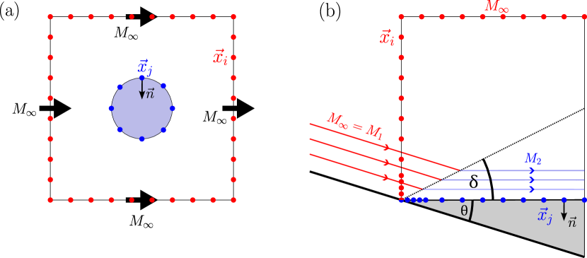
Figure 2: Schematic representation of boundary conditions and boundary training points for the cylinder and the oblique shock test case. The Dirichlet boundary conditions for a Mach number of $M_{\infty}$ are applied at the points $\bm{x}_{i}$ with $i=1\dots N_{\infty}$. The wall boundary conditions at the obstacle surfaces are enforced at the points $\bm{x}_{j}$ with $j=1\dots N_{\mathrm{ob}}$. Note that for the parametric problems, one additional sampling dimension per parameter is appended to the euclidean spatial coordinates.

2.2.1 Adaptive Artificial Dissipation

A fundamental challenge for PINNs in the search of solutions to the compressible Euler equations lies in finding a physically reasonable minimum of the loss (i.e. an entropy solution). By definition of the loss function (3), any weak solution of Eqs. (7) that fulfills a given set of boundary conditions is a (global) minimum of the loss and thus a possible final state of the network to converge to. Furthermore, the optimizer can always converge to local minima, which correspond to unphysical solutions.

In classical computational methods for the solution of compressible flows, artificial dissipation is introduced in the form of upwind schemes or through a combination of central schemes and explicit dissipative terms [1]. The dissipation smears out discontinuities and has a stabilizing effect.

For PINNs, the necessity of additional dissipative terms for successfully solving scalar conservation laws has also been observed by Fuks et al. [34]. More complex systems of conservation laws, such as the compressible Euler equations require advanced methods for locally determining reasonable dissipation levels while also minimizing the dissipative effects on the solution.

Here we propose a novel training procedure for flexibly and reliably solving the compressible Euler equations which uses artificial dissipation. The novelty of this procedure is twofold. Firstly, the PINN locally predicts an appropriate value of viscosity which is necessary to stabilize the training. Secondly, the strength of dissipation is reduced during the training process which minimizes errors that are introduced by the dissipation.

The dissipation is introduced as an additional term in Eqs. (7):

$$\partialderivative{\bm{W}}{t}+\partialderivative{\bm{F}_{x}}{x}+\partialderivative{\bm{F}_{y}}{y} =\eta\Delta\bm{W}$$ (10)

where $\Delta=(\partial_{x}^{2}+\partial_{y}^{2})$ is the Laplacian and $\eta$ can be interpreted as an artificial viscosity. From an optimization point of view, the dissipation acts as a regularization of the optimization/training problem. Similarly to classical scalar dissipation schemes like the JST-scheme [45], we scale the dissipation locally, based on the spectral radius of the flux jacobians

$$\eta=\nu(a+|\bm{q}|)$$ (11)

where $\nu$ is a viscosity factor for which adequate values have to be selected. The linear scaling of the viscosity $\eta$ with the wave speed $a+|\bm{q}|$ results in higher viscosity values in regions with higher Mach numbers. Furthermore, when considering parametric problems with variable inflow velocities, the viscosity is adjusted according to the resulting variable wave speed. However, additional local upscaling of the viscosity may be required to deal with certain highly nonlinear or unstable regions in the domain, such as shocks. Instead of deriving an analytical sensor function, we leverage the ability of the neural network to adjust the viscosity. To do so, the network predicts the viscosity factor $\nu$ alongside the primitive variables $\bm{\hat{u}}(\bm{\theta},\bm{x})\approx(\rho(\bm{x}),u(\bm{x}),v(\bm{x}),E(\bm{x}),\nu(\bm{x}))$. To enforce positivity of the viscosity and to allow for a flexible prediction of values close to 0, the exponential function is used as an activation for $\nu$ in the last layer of the network. In addition, since we are interested in the inviscid solution, an additional loss term $\mathcal{L}_{\nu}$ is introduced which penalized high viscosity values :

$$\mathcal{L}_{\nu}=\gamma|\nu-\tilde{\nu}|.$$ (12)

The prescribed viscosity value $\tilde{\nu}$ can now be used to control the strength of the dissipative term, while still allowing the network to locally choose $\nu(\bm{x})\neq\tilde{\nu}$ when necessary. We use the modulus to enforce positivity of the term instead of the square because local outliers should not be penalized. We want to stress that $\tilde{\nu}$ is not related to a turbulent eddy viscosity for which this symbol is oftentimes used in turbulence models.

The addition of dissipation changes the physical problem and the resulting solution will disagree with the fully inviscid solution. Essentially, one is no longer solving for an inviscid solution and therefore the fluid is decelerated by shear stresses. In classical methods, scalar dissipation schemes employ fourth order differences in smooth flow regions which only dampens higher frequency modes of the flow, limiting the effect of the artificial viscosity on the solution. Second order differences are only used near discontinuities, where a scheme of first order accuracy is required due to Godunov’s theorem. An additional fourth order differential term could theoretically be added to Eq. (10). This would however introduce fourth order derivatives which would require additional expensive evaluations of the computational graph. Instead, we follow a different approach and adjust the viscosity during the training process, to limit the dissipative effect on the final solution. Therefore, we propose a 3 phase training routine:

• Phase 1: Train with ADAM at a constant viscosity $\tilde{\nu}=\nu_{0}$ until no significant changes in the residual loss are observed.

• Phase 2: Train with ADAM and reduce the prescribed viscosity $\tilde{\nu}$ until $\tilde{\nu}=0$. Continue at $\tilde{\nu}=0$ until no significant changes in the residual loss are observed.

• Phase 3: Train with LBFGS and $\tilde{\nu}=0$ until convergence.

The idea of this procedure is to guide the network towards a physical solution (the entropy solution) during the initial training phase. Once the network has converged to a state that resembles a physical but viscous solution, the viscosity can be reduced, since, from this point on, the network should be in a state near the entropy solution. In phase 2, $\tilde{\nu}$ is reduced to 0, to decrease the dissipative effect on the prediction. However, the network can still predict viscosity factors $\nu(\bm{x})>0$ where necessary, keeping the penalty term in balance with the residual and other loss terms. We reduce the prescribed viscosity factor $\tilde{\nu}$ as follows:

$$\tilde{\nu}_{i}=\begin{cases}\nu_{0}\bigg{(}1-\bigg{(}\frac{i}{M_{\mathrm{red}}}\bigg{)}^{k}\;\bigg{)}&\text{if}\;\;0\leq i\leq M_{\mathrm{red}}\\ 0&\text{if}\;\;M_{\mathrm{red}}<i\end{cases}$$ (13)

Where $i\in\mathbb{N}$ is the epoch counter starting at phase 2 and $M_{\mathrm{red}}$ is the epoch at which $\tilde{\nu}=0$ is reached. The exponent $k\in\mathbb{N}^{+}$ can be used to modify the shape of the reduction curve. For $k=1$ the reduction is linear and for $k>1$ it is accelerating. For the first two phases, Adam [40] is used as the optimizer. A final training period with the quasi-Newton LBFGS optimizer [46] has shown to be effective for convergence of PINNs in general and has been crucial to achieve high levels of accuracy with the proposed training procedure. A schematic representation of the described PINN approach is shown in Fig. 1 and a schematic view of the boundary points for the later discussed test cases is shown in Fig. 2.

3 Parametric Flow around Ellipse

As the first parametric problem we consider the flow around an ellipse with a parametric inflow boundary condition and a parametric ellipse boundary. We position the two-dimensional ellipsoid at the center of the domain $\Omega=(-1,1)\times(-1,1)$. The semi-major axis $a\in(0.1,0.2)$ is variable whereas the semi minor axis $b=0.1$ is constant. Therefore at a value of $a=0.1$, we have a cylinder of radius $r=0.1$ which corresponds to an eccentricity of $e=\sqrt{1-b^{2}/a^{2}}=0$. For the maximal major axis of $a=0.2$ the eccentricity is $e=3/4$. As a second varying parameter we consider the Mach number $M_{\infty}\in(0.2,0.4)$. The neural network receives both parameters as additional inputs. The training points are therefore sampled in a four-dimensional domain. The upper limit of the Mach number of $M_{\infty}=0.4$ is slightly below the critical Mach number of the cylinder, at which the velocity locally exceeds the speed of sound. An initial prescribed artificial viscosity factor of $\nu=7.5\cdot 10^{-4}$ is used based on the previous investigations. We have observed that this value is typically a reasonable value and can be used both for subsonic and supersonic problems. Since the actual artificial viscosity in Eq. (11) is scaled with the local wave speed, the strength of the dissipation naturally increases at higher Mach numbers.

We choose a fully connected neural network of constant layer width. We investigate the performance of fixed and adaptive hyperbolic tangent activation functions. We observe that during the third training phase, when using the LBFGS optimizer, the usage of adaptive activation functions leads to highly inconsistent results (i.e. in some runs convergence is similarly to $\tanh$ and in others no further convergence is possible or the optimizer diverges completely). Therefore, we decide to freeze the trainable parameters $\omega^{k}$ for the final training phase meaning that these parameters are no longer optimized during phase 3. In doing so, we are able to avoid the previously observed inconsistencies.

The loss weighting factors are set to $\beta=1$ and $\gamma=5$. As shown in various publications, such as [47, 18, 19], the (dynamic) weighting of loss terms is an effective technique to accelerate the convergence and improve the accuracy because it can compensate imbalances in the gradients between the different loss terms. However, we have observed that for certain problems, adaptive loss term weighting may lead to instabilities during the early stages of the training. For the presented problems we do not see significant imbalances during the training and are able to achieve satisfying results with a constant weighting factor. Therefore, dynamic loss term weighting is not considered herein.

A summary of all hyperparameters is shown in Tab. 2. This includes the utilized optimizer, the learning rate $lr$ the batchsize $N_{\mathrm{batch}}$ and the prescribed viscosity factor $\tilde{\nu}$. To cover the four-dimensional input space, the number of residual training points is comparatively high ($N=100000$). However, since a mini-batch routine is used for the first two training phases, this has typically no negative effect on the training speed. Only during the last training phase 3, memory may be a limiting factor because the LBFGS optimizer is incompatible with mini-batch training. Therefore, we use a reduced number of training points during the last training phase ($N=30000$). A non-uniform point distribution is used. Half of the points are distributed uniformly across the entire physical domain $\Omega=(-1,1)\times(-1,1)$ using the Halton sequence [38]. For the other half of the points, the y-coordinate is sampled using a normal distribution with a variance of $\sigma=0.07$ and with a uniform distribution for the x-coordinate. A projection of the resulting point distribution to the physical domain is shown in Fig. 4. For both point sets, the same number of points is used to represent the boundary of the physical domain and the cylinder ($N=N_{\mathrm{\infty}}=N_{\mathrm{ob}}$). No additional data of the solution is incorporated into the loss, besides the boundary conditions. We are thus approximating the solution of a fully determined (but not over-determined) forward problem. The resulting predictions for the velocity field for three cases are shown in Fig. 5 in comparison to reference finite volume simulations. For additional information on the calculation of reference finite volume results, see Sec. C. One can see that for the cylindrical shape ($a=0.1$) even at $M_{\infty}=0.4$, close to the critical Mach number, the results are visually indistinguishable to the reference solution. The plot of the absolute error reveals that the inaccuracies are fairly uniform. For the other two parameter sets with ellipsoidal shapes, a similar quality of the results can be observed. The bottom row of Fig 5 depicts the artificial viscosity $\eta$. The viscosity is relatively uniform (see the scale of the color bars) for all three Mach number. Up and downstream of the ellipse, the viscosity is however slightly reduced.

For certain problems it can be observed that PINNs can perform inconsistently, depending on the random initialization of network parameters at the start of the training. To ensure the consistency of our proposed method we analyze the accuracy over 12 training runs with different random initialization seeds. Fig. 6 (a) shows the mean error in the density field during training. The best and worst prediction accuracy over the 12 runs (i.e. the spread of the predictions) is also indicated. While differences occur between different initializations during early training phases, all models converge to a similar final accuracy. Fig. 6 (b) shows the prescribed viscosity factor $\tilde{\nu}$ as well as the predicted mean viscosity $\nu$ during training. Besides a spike in the first few epochs, the prescribed and predicted viscosity are identical during the first phase. In phase 2 we see that the viscosity is comparatively quickly reduced. After about 2500 epochs, it remains at a constant value around $\nu=10^{-6}$. This indicates that this lower viscosity is sufficient for stabilizing the training and that $\nu$ can be reduced relatively fast during phase 2 without causing any instabilities. This is to be expected for this relatively stable subsonic problem. However, as shown in A.1, the initial viscosity in phase 1 is still required to converge to reasonable predictions which is even apparent for the non-parametric version of the problem. On average we can only observe marginal improvements in accuracy and convergence speed, when using adaptive activation functions instead of the fixed hyperbolic tangent activations. For a quantitative assessment of the errors, we consider the pressure coefficient $C_{\mathrm{p}}$, the local Mach number $M$ and the density $\rho$ for 100 quasi-random parameter values in the parameter space. For each parameter set, the mean absolute difference to the reference solution was calculated for a small square that contains the cylinder ($-0.5<x<0.5;-0.5<y<0.5$). Fig. 3 shows the resulting absolute errors for the density. These errors are then normalized with the range of values of the reference solution for each individual quantity. The final relative errors in Tab. 1 are the mean over all datasets and all 12 runs. The relative errors confirm that adaptive and non-adaptive activation functions perform very similarly for this example.

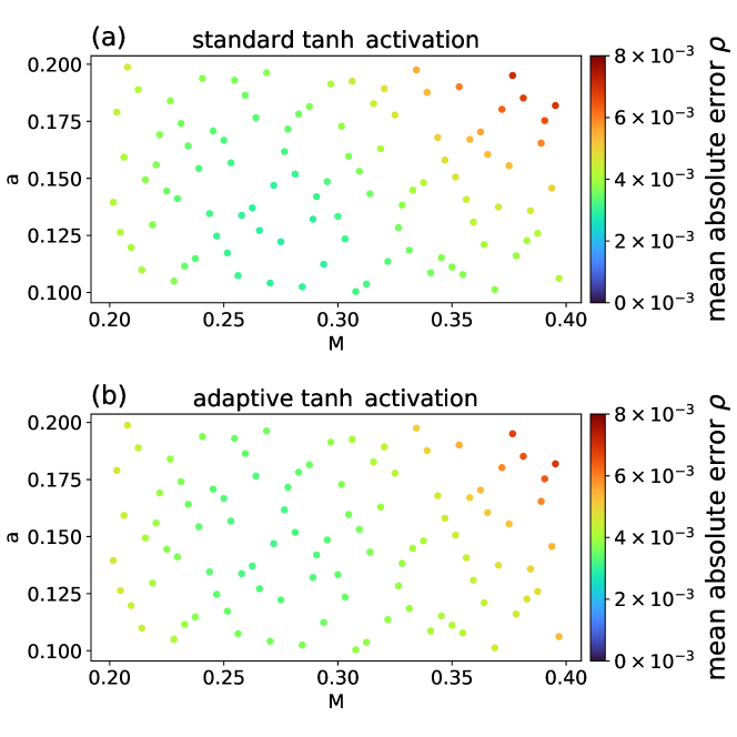
Figure 3: (updated) Mean absolute errors on subsonic test case between parametric PINN and reference finite volume result for the density field, for different parameter sets. Fig. (a) shows the results without and Fig. (b) with adaptive $\tanh$ activation functions.

For a detailed explanation of the error calculation see Sec. C. The hyperparameters are not optimized and higher accuracies may be possible when employing hyperparameter optimization e.g. on the network shape and learning rate.

For all presented results, the Python package SMARTy [48] was used, which is a toolbox for surrogate modeling and other data driven tasks. SMARTy supports Tensorflow and PyTorch as backends for the creation and training of neural network models. With the tensorflow backend the model is trained in 24 hours on a single NVIDIA A100 graphics card. All the presented models were using double precision for the floating point numbers. Once trained, the evaluation of the model is fast. The prediction of the model at $300.000$ points takes about $0.5\;\mathrm{s}$.

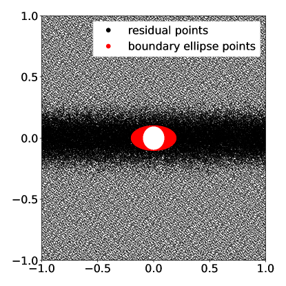
Figure 4: Projection of point distribution of four-dimensional parametric space onto physical domain for subsonic ellipse problem. Note the variation in the axis $a$ in the boundary points.

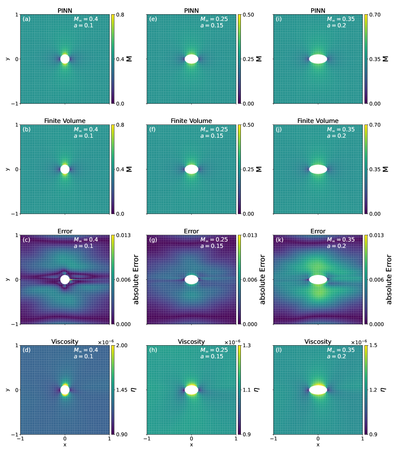
Figure 5: (updated) Comparison between parametric PINN solution with adaptive activation functions and a reference finite volume result for different Mach numbers and ellipse eccentricities. The absolute errors between the reference and the PINN solution are shown in Figs. (c), (g) and (k). Figs. (d), (h) and (l), show the artificial viscosity $\eta$.

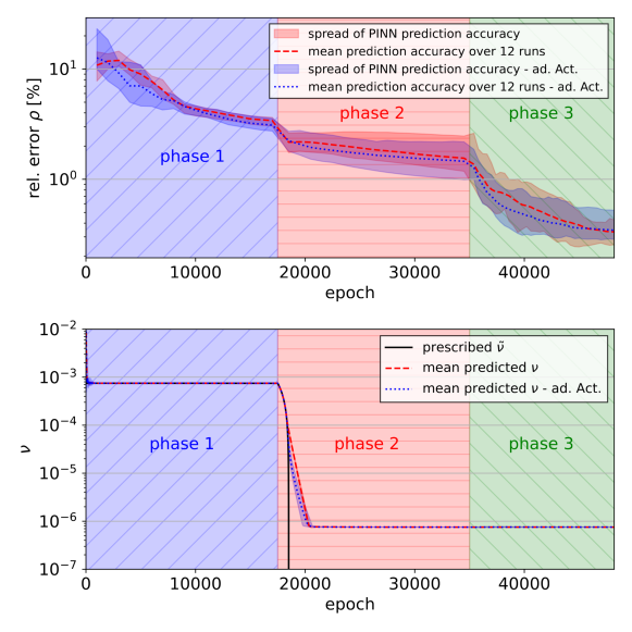
Figure 6: (updated) Error, prescribed and predicted viscosity during training for flow around ellipse. Fig (a) also shows the spread of prediction accuracy for 12 random initializations of the network.

4 Parametric Oblique Shock

As a supersonic test case we consider the Oblique Shock problem with a variable inflow Mach number of $M\in(2,3)$. The test case describes a scenario where a supersonic inflow is deflected by a wedge with deflection angle $\theta=10^{\circ}$. The resulting attached shock originates from the corner of the wedge. We define the shock angle with respect to the surface of the wedge as $\delta$. The shock angle is a unique function of the deflection angle and the incoming Mach number $M_{1}=M_{\infty}$ as stated by the $\theta$-$\beta$-$M$ relation. The field variables after the shock can be calculated analytically from $M_{1}$ and $\theta$ [49].

This problem has been solved with PINNs in a non-parametric version with $M=2$ in [31] and [22]. For a comparison of the non-parametric results with and without adaptive viscosity, see A. To the best of our knowledge this is the only other forward supersonic test case which has been solved with PINNs for the two-dimensional compressible Euler equations. PINNs have however been applied to other inverse supersonic problems [32] where shock locations are already given by solution data that is provided inside of the physical domain.

Here, we solve the forward problem in the continuous parameter space for $M_{\infty}=(2,3)$. We use a total of $100000$ points for the evaluation of the residual and the viscosity penalty loss. $80000$ of these points are uniformly sampled in the three-dimensional input space $(x,y,M_{\infty})\in\Omega\times(2,3)=(0,1)\times(0,1)\times(2,3)$. An additional 10.000 points are uniformly sampled on the upper $(x,y,M_{\infty})\in\Omega\times\{3\}$ and lower bound $(x,y,M_{\infty})\in\Omega\times\{2\}$ of the parameter space to enhance the accuracy towards the borders. The Halton sequence [38] is used for generating all three point sets. Note that, in contrast to previous works, we do not require clustered training points [31] or domain decomposition [22] for accurate predictions. This is advantageous, because no previous knowledge of the solution is required for the point generation or for the decomposition. Dirichlet boundary conditions are applied at the top and left surface. No-flux wall boundary conditions are used for the bottom boundary. Since the shock originates from the bottom left corner, we increase the boundary point density for $x\in(0,0.1)$ and $y\in(0,0.1)$ as sketched in Fig. 2. As before, an initial prescribed viscosity factor of $\tilde{\nu}=7.5\cdot 10^{-4}$ is used. The network consists of 7 layers with layers of 30 neurons and $\tanh$ activations. We compare fixed and adaptive hyperbolic tangent activation functions but freeze the trainable parameters of the activations in phase 3 as explained in Sec. 3. The loss term weights are $\beta=1$ and $\gamma=5$. A detailed overview of training parameters is shown in 3. Again, no additional data of the solution is incorporated into the loss, besides the boundary conditions and we are strictly solving the forward problem.

Fig. 7 provides an overview of the result for three different Mach numbers in comparison to the analytical solution. The field values before and after the shock are accurately predicted and the shock is well resolved. Slight inaccuracies in the shock angle are visible. The bottom row shows the artificial viscosity. Due to the local adaptivity, the dissipation is increased close to the shock. This shows that the proposed method is able to locally identify regions which require additional viscosity for stabilization. In this sense, the network is able to take over the role of so called pressure sensors, which are used in classical CFD methods to switch to first-order schemes near shock locations. Since PINNs can perform inconsistently, depending on the random initialization of network parameters at the start of the training, we analyze the accuracy over 12 training runs with different random initialization seeds. The following plots highlight the mean prediction over those 12 runs and the largest and smallest values (i.e. the spread of the predictions). The usual quantities like standard deviation and quantiles are not calculated due to the limited number of 12 training runs. As an integral indicator of prediction accuracy we consider the shock angle $\delta$ (see Fig. 2). Fig. 8 shows an overview of predicted shock angles for the entire parameter space. Overall the error of the shock angle is lower than one degree. The errors are larger at the lower bound of the parameter space towards $M_{\infty}=2$. The spread of the predictions over the 4 training runs indicates that the results are generally within a one degree neighborhood of the analytical solution both with and without adaptive activation functions. In this example, one can see that the adaptive outperform the fixed activation functions. Fig. 9 (a) shows how the error for the angle delta changes during the training. We see that the error in the angle does not improve significantly after phase 1 and that the spread of predicted angles in fact increases. However, Fig. 10 shows that during the second and third training phase, the shock becomes much sharper and thus approximates the expected analytical result better. This is also confirmed by the decrease in the relative density errors (see Fig. 9 (b)). Note that the final training phase 3 with LBFGS is crucial to obtain good accuracy. The error history shows that on average, the adaptive activation functions can accelerate convergence in phase 1 and 2. In phase 3 the most inaccurate runs with and without adaptive activations are very similar, while the most accurate runs are improved for the adaptive activations. Fig. 9 (c) shows the prescribed viscosity value $\tilde{\nu}$ and the mean (over the domain) predicted viscosity $\nu$ during the training. Contrary to the subsonic test case we can clearly see the adaptivity of viscosity and how it is only loosely coupled to the prescribed value. Early in the training we can see an adaptive increase beyond the prescribed value which is accompanied by a fast convergence during the first few thousand epochs. Then, during phase 2, the predicted viscosity is again reduced less steeply than the prescribed value which indicates that more viscosity is necessary than prescribed, to stabilize the training during the reduction phase. During phase 3 the predicted viscosity decreases more steeply. The final values are between $\nu=2\cdot 10^{-5}$ and $\nu=2\cdot 10^{-6}$ and thus higher than for the subsonic test case. The viscosity for the adaptive activations is on average slightly increased. The necessity for more viscosity during the training is to be expected since we are dealing with a supersonic flow that involves a shock. Compared to the previous subsonic test case, this problem should be more unstable and require more dissipation.

For a quantitative comparison of relative errors with the subsonic problem, we again consider the pressure coefficient $C_{\mathrm{p}}$, the local Mach number $M$ and the density $\rho$ for 20 linearly distributed Mach number values with $M\in[2,3]$. For each parameter, the mean absolute difference to the reference solution was calculated for the entire domain. This difference was then normalized with the range of values of the reference solution for each individual quantity. The calculation of errors and uncertainties is described in more detail in Sec. C. The hyperparameters are not optimized and higher accuracies may be possible when employing hyperparameter optimization e.g. on the network shape and learning rate. The use of adaptive activations generally leads to improved accuracies, especially for the Mach number $M$. Compared to the subsonic problem 3, we see slightly increased errors within the same order of magnitude. The bounds of the error are higher, mainly due to the fact that accuracies are worse close to the lower Mach number $M=2$, while the errors of the subsonic problem are consistently low for the entire parameter space (c.f. Sec. C).

Again, the models are implemented with SMARTy [48] using the tensorflow backend and the total training time for one run on a NVIDIA A100 graphics card is about 23 hours. The prediction at $300000$ points takes about $0.5\;\mathrm{s}$.

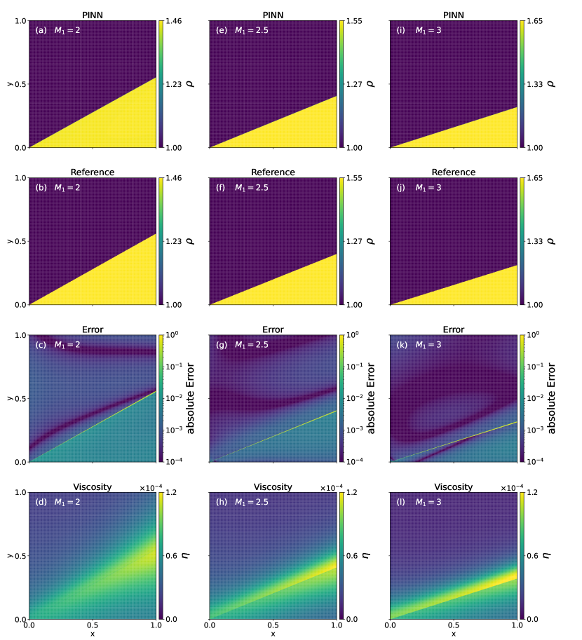
Figure 7: (updated) Comparison of parametric PINN solution using adaptive actiation functions for oblique shock test case with the analytical reference solution for different Mach numbers. The absolute errors between the reference and the PINN solution are shown in Figs. (c), (g) and (k). Figs. (d), (h) and (l), show the artificial viscosity $\eta$.

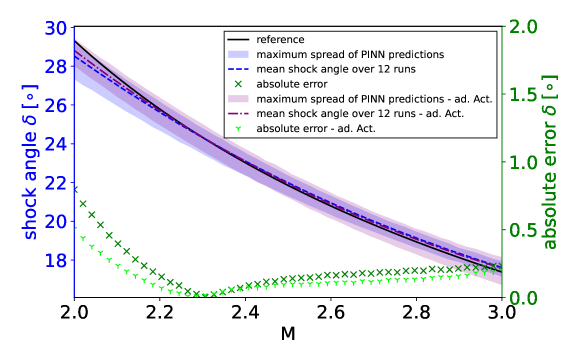
Figure 8: (updated) Mean and spread of predicted shock angles. The blue curves show the angle $\delta$ (for the definition see Fig. 2). The green curve shows the absolute error which is the absolute difference between the two blue curves.

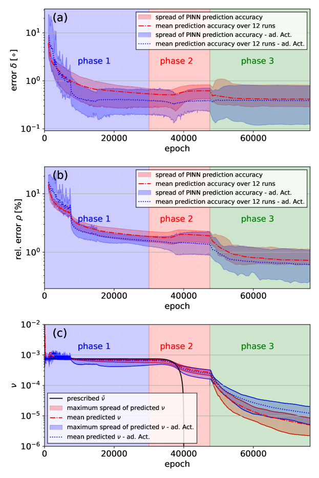
Figure 9: (updated) Error history and artificial viscosity factor $\nu$ during training of PINN for parametric oblique shock problem. The three phases of the applied training procedure are highlighted.

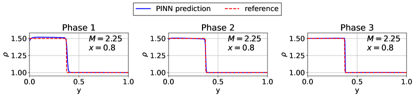
Figure 10: (updated) Exemplary cross-section through density field at $M_{\infty}=2.25$ shows how shock becomes less dissipative after reducing the viscosity during the training. Results were obtained using the adaptive activation functions.

Table 1: (updated) Comparison of relative errors for different field variables.

Sec.	3. Parametric Flow around Ellipse		4. Parametric Oblique Shock
	$\sigma$	$\sigma_{\mathrm{adapt}}$	$\sigma$	$\sigma_{\mathrm{adapt}}$
$C_{\mathrm{p}}$	$(0.23\pm 0.06)\%$	$(0.25\pm 0.08)\%$	$(0.7\pm 0.7)\%$	$(0.52\pm 0.61)\%$
$M$	$(1.0\pm 0.1)\%$	$(1.0\pm 0.11)\%$	$(1.3\pm 0.9)\%$	$(0.7\pm 0.7)\%$
$\rho$	$(0.33\pm 0.11)\%$	$(0.34\pm 0.13)\%$	$(0.62\pm 0.62)\%$	$(0.5\pm 0.6)\%$

5 Conclusion

To summarize, we propose a novel physics-informed neural network training procedure to approximate parametric solutions to the stationary compressible Euler equations. Parameters are considered as additional input dimensions of the network. Furthermore, we add a dissipative term to the equations to stabilize the training process. Our proposed method locally predicts the necessary viscosity. An additional penalty loss term is used to control and reduce the viscosity during the training so that the resulting solution is non-dissipative. We obtain accurate results on a subsonic test case with a parametric Mach number and boundary shape as well as a supersonic test case with parametric Mach number. Adaptive activation functions perform similar on the subsonic test case and outperform the fixed activation functions on the supersonic test case. The proposed method is easy to implement and outperforms vanilla PINNs without viscosity (c.f. A) which have so far rarely been applied successfully, for more than one-dimensional forward problems governed by the Euler equations without requiring previous solution knowledge (e.g. for data, clustered points or solution based domain decomposition). Thus, the presented method may open up new possibilities for the use of PINNs for similar inviscid problems, which were previously unsolvable, using vanilla PINNs. Compared to finite volume reference simulations, we achieve errors on the order of less than $2\%$ for the pressure, velocity and density field, for both test-cases while using no additional data besides boundary conditions.

While the shown results are overall promising, one might consider the training cost to be a limiting factor of the method. The viscous term introduces additional, second-order derivatives which increase the computational effort per epoch due to additional automatic differentiation calls. In addition, the used neural networks have to be comparatively large because they need to capture the solution of four field variables and the artificial viscosity factor. With regards to the additional training cost due to the viscous term, we consider this to be a sensible compromise because, as seen in A, convergence without viscous terms seems to be unreliable at best. This is to be expected due to the mathematical nature of hyperbolic conservation laws and we know from classical numerical methods that additional stabilizing methods such as artificial viscosity are required to obtain unique and physical solutions. In the future we plan to reduce the network size by decomposing the domain into subsets which are appoximated by smaller individual networks. Even though we obtain accurate solutions with a global network for the entire domain, we expect that domain decomposition will be able to further increase the accuracy, enable faster parallel training and to reduce the requirements for network size. Especially for larger domains, as well as transient and higher-dimensional problems, domain decomposition approaches may be imperative because very large global networks are limited in resolving local effects and training convergence becomes increasingly difficult. Fortunately, since our methodology just requires the network to predict the local viscosity factor $\nu$ and a simple modification of the loss function, it can easily be incorporated into existing domain decomposition frameworks. Decomposition methods with explicit interface losses, such as extended PINNs [23], would require additional continuity conditions for the viscosity factor at the domain interfaces. Therefore, soft domain decomposition approaches such as augmented PINNs [25] or finite basis PINNs [26] might be favorable. Overall , we see various possibilities to further improve numerical efficiency of the described approach in the future. Moreover, we also have to take into account that inference times are on the order of $1\;\mathrm{s}$ and that due to the parametric formulation, one is able to obtain solutions for different parameter conditions with a single trained PINN model. This makes parametric PINNs viable in specific scenarios which require real-time evaluation. The proposed implementation of artificial viscosity is simplistic and one can think of many ways to improve this approach. Similarly to artificial matrix-valued artificial viscosity schemes in classical CFD methods [50, 51, 52, 53], a yet to be developed matrix-valued viscosity model for $\eta$ might reduce the influence of the dissipative term during training, while maintaining its stabilizing properties. Also, an alternative regularization scheme based on an entropy criteria has been proposed for solving hyperbolic problems with PINNs which might be an additional measure to avoid unphysical results, when solving the compressible Euler equations, especially at higher Mach numbers [54, 32]. However, our initial tests indicate that this methodology is not sufficient to stabilize our analyzed forward problems on its own.

The presented approach of parametric boundary conditions can, in theory, be extended to more parameters (e.g. with variable Mach number, shape and angle of attack for airfoils). Therefore, it could be applicable for tasks such as design optimization which traditionally require many solver evaluations. Whether a sufficient level of accuracy can be reached for more complex multi-parameter problems remains to be seen. An aspect of PINNs that has not been considered in this work is that higher fidelity solution data can be incorporated into the objective function as an additional loss term. This opens the possibility to directly combine PINNs with classical solvers or to even incorporate experimental data into the loss. For parametric problems, such a hybrid-data-driven approach may improve accuracy and even speed up the convergence during training. This flexibility may open up new possibilities for physics-informed reduced order modeling for higher dimensional parametric flows.

An additional point of future interest is the behavior of the presented approach in the transsonic regime, where velocities exceed the speed of sound only locally. Furthermore, we want to consider transient problems. We expect that this requires additional measures like decomposition of the temporal domain (see e.g. [55]) while respecting temporal causality. For transient problems we expect long training times because, when employing causality preserving temporal decomposition strategies, every temporal subdomain has to go through the training phases 1-3 successively, to avoid an accumulation of viscous effects over time.

Appendix A Non-Parametric Problems

To highlight the necessity and the efficacy of artificial viscosity, we consider non-parametric versions of the previously analyzed problems and compare the results with and without adaptive artificial viscosity.

A.1 Flow around Cylinder

First, we investigate the flow around a cylinder at a constant Mach number of $M=0.2$. Again, the center of the cylinder is positioned at the origin inside the domain $\bm{x}=(x,y)\in\Omega=(-1,1)\times(-1,1)$ with a radius of $r=0.1$. Fig. 11 (c) show a numerical reference solution of the problem for a Mach number of $\mathrm{M}=0.2$. The solution was obtained using the CFD solver CODA [4]. For additional information on the calculation of reference finite volume results, see C.

Similarly to before, no-flux boundary conditions are used for the cylinder wall and Dirichlet boundary conditions are enforced using Eq. (9) for the external domain boundary. A summary of the parameters within each training phase is shown in Tab. 2. For the PINN without viscosity, we train for the same number of epochs with the ADAM and LBFGS optimizer as for the model with adaptive viscosity. The learning rate for ADAM is however set to $lr=10^{3}$ for the entirety of the ADAM training. All other hyper parameters and the training points are identical
The training points for the residual loss are randomly sampled in the entire domain, using the quasi-random Halton sequence [38]. For both point sets, the same number of points are used to represent the boundary of the physical domain and the cylinder ($N=N_{\mathrm{\infty}}=N_{\mathrm{ob}}$).

Figs. 11 (a)-(b) show the resulting velocity fields given by the local Mach number. The training parameters correspond to phase 1 in Tab. 2 . The results without adaptive viscosity shows elongated, unphysical regions of low velocity before and after the cylinder. In comparison, the model with adaptive viscosity agrees well with the reference simulation.

The training with SMARTy [48] and the tensorflow backend on a single NVIDIA A100 graphics cars takes about $6$ hours without viscosity and about $11$ hours for the model with viscosity, due to the increased effort for calculating the loss function.

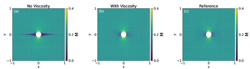
Figure 11: Comparison of PINN predictions for the local Mach number $M$ with and without artificial viscosity and the reference finite volume simulation.

A.2 Oblique Shock

We consider the oblique shock at a incoming Mach number of $M_{\infty}=2$. The training points for the residual loss are generated similarly to Sec. 4 with the Halton sequence inside ob the physical domain $(x,y)\in\Omega=(0,1)\times(0,1)$. Dirichlet boundary conditions are used for the left and upper boundary and no-flux wall conditions are used for the bottom boundary. No boundary condition is used on the right boundary.

This exact forward problem has been solved with PINNs in [31] and conservative PINNs in [22]. Hence, to demonstrate the efficacy of artificial viscosity, we try to reproduce the reported results of [31] by selecting similar hyper parameters for the neural network shape (7 layers with 20 neurons) and a similar number of uniformly distributed points (5000 for the residual loss) and compare the predictions with and without the adaptive viscosity for these exact hyper parameters. Note that we use uniformly distributed and no clustered training points because we do not want to assume any previous knowledge about the solution and the shock angle. We do however increase the boundary point density in the bottom left corner at the shock origin as schematically depicted in Fig. 2. Also the number of points on the boundaries overall increased to 2000, compared to 300 points in [31]. Again, both PINN models with and without adaptive viscosity are trained for the same number of ADAM epochs (phase 1 and 2 combined for the viscous PINN) and LBFGS epochs.

Fig. 12 shows the resulting density fields.

We are unable to obtain similar results for the inviscid PINN as shown in [31] even though the number of boundary points and the number of ADAM epochs have been increased. We have also searched for better hyper parameters and even employed adaptive activation functions and dynamic loss term weighting but were still unable to obtain qualitatively improved results. Nevertheless, even when compared to the shown results in [31], we obtain highly improved results using the proposed adaptive viscosity during training. The shock is much sharper and less dissipative, even without clustered training points.

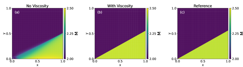
Figure 12: Comparison of results for the non-parametric oblique shock problem at $M_{\infty}=2$. The local Mach number $M$ is shown for training runs with (Fig. (b)) and without (Fig. (a)) adaptive artificial viscosity in comparison to the reference finite volume result (c). The hyper parameters used for (a) and (b) are the same. A search for better hyper parameters for (a) has not lead to significant improvements even when employing dynamic loss term weighting [18, 19, 47] or adaptive activation functions [43].

Appendix B Training Parameters

Table 2: (updated) Summary of PINN parameters for flow around ellipse.

Sec.	A.1. Flow around Cylinder	3. Parametric Flow around Ellipse
hidden layers	$8$	$8$
neurons/layer	$20$	$40$
activation	(adapt.) $\tanh$	(adapt.) $\tanh$
loss weights	$\beta=1$ $\gamma=5$	$\beta=1$ $\gamma=5$
phase 1	Adam $\tilde{\nu}=7.5\cdot 10^{-4}$ $N=20000$ $N_{\mathrm{batch}}=2500$ $10000$ epochs w. $lr=10^{-3}$ $20000$ epochs w. $lr=10^{-4}$	Adam $\tilde{\nu}=7.5\cdot 10^{-4}$ $N=100000$ $N_{\mathrm{batch}}=10000$ $7500$ epochs w. $lr=10^{-3}$ $7500$ epochs w. $lr=10^{-4}$ $2500$ epochs w. $lr=10^{-5}$
phase 2	Adam reduce $\tilde{\nu}=7.5\cdot 10^{-4}$ to $\nu_{0}=0$ $N=20000$ $N_{\mathrm{batch}}=2500$ $M_{\mathrm{red}}=2500$ $k=4$ $5000$ epochs w. $lr=10^{-4}$ $5000$ epochs w. $lr=10^{-5}$	Adam reduce $\tilde{\nu}=7.5\cdot 10^{-4}$ to $\nu_{0}=0$ $N=100000$ $N_{\mathrm{batch}}=10000$ $M_{\mathrm{red}}=1000$ $k=1$ $17500$ epochs w. $lr=10^{-5}$
phase 3	LBFGS $\tilde{\nu}=0$ $N=5000$ $25000$ epochs	LBFGS $\tilde{\nu}=0$ $N=30000$ $30000$ epochs

Table 3: (updated) Summary of PINN parameters for oblique shock problem.

Sec.	A.2 Oblique Shock	4. Parametric Oblique Shock
hidden layers	$7$	$7$
neurons/layer	$20$	$30$
activation	(adapt.) $\tanh$	(adapt.) $\tanh$
loss weights	$\beta=1$ $\gamma=5$	$\beta=1$ $\gamma=5$
phase 1	Adam $\tilde{\nu}=7.5\cdot 10^{-4}$ $N=5000$ $N_{\mathrm{batch}}=N$ $12000$ epochs w. $lr=10^{-3}$ $18000$ epochs w. $lr=10^{-4}$	Adam $\tilde{\nu}=7.5\cdot 10^{-4}$ $N=100000$ $N_{\mathrm{batch}}=10000$ $7500$ epochs w. $lr=5\cdot 10^{-4}$ $7500$ epochs w. $lr=10^{-4}$ $15000$ epochs w. $lr=2\cdot 10^{-5}$
phase 2	Adam reduce $\tilde{\nu}=7.5\cdot 10^{-4}$ to $\nu_{0}=0$ $N=5000$ $N_{\mathrm{batch}}=N$ $M_{\mathrm{red}}=5000$ $k=1$ $20000$ epochs w. $lr=2\cdot 10^{-5}$	Adam reduce $\tilde{\nu}=7.5\cdot 10^{-4}$ to $\nu_{0}=0$ $N=100000$ $N_{\mathrm{batch}}=10000$ $M_{\mathrm{red}}=10000$ $k=4$ $17500$ epochs w. $lr=2\cdot 10^{-5}$
phase 3	LBFGS $\tilde{\nu}=0$ $N=5000$ $10000$ epochs	LBFGS $\tilde{\nu}=0$ $N=20000$ $30000$ epochs

Appendix C Details on Reference Simulations, Calculation of Errors and Shock Angles

C.1 Parametric Flow around Ellipse

All reference simulations for the ellipse were calculated using CODA [4, 56]. CODA is the computational fluid dynamics (CFD) software being developed as part of a collaboration between the French Aerospace Lab ONERA, the German Aerospace Center (DLR), Airbus, and their European research partners. CODA is jointly owned by ONERA, DLR and Airbus. We use a structured O-type grid with 200 surface nodes and 13200 cells. The residuals are converged to an order of $10^{-12}$. For a quantitative evaluation of the accuracy of the parametric PINN in Sec. 3, we compare the solutions to 100 reference finite volume simulations in the parameter space $(M,a)\in(0.2,0.4)\times(0.1,0.2)$. The parameter sets sampled using the Halton sequence [38]. Fig. 3 shows the parameter values and the absolute errors for the density field. For each parameter set, the errors are calculated for each field variable separately, by taking the mean of the absolute difference over a small rectangle $(x,y)\in(-0.5,0.5)\times(-0.5,0.5)$ near the ellipse. The figure then depicts the mean error over all training runs. Overall the errors are all on the same order of magnitude and we see no significant outliers in the entire parameter space. The results are less accurate towards the bounds of the parameter space.

For the calculation of the relative errors in Tab. 1 and Fig. 6 the previously calculated absolute errors are normalized with the range of the respective field variable, taken from the reference simulations. Then the mean over the parameter sets is taken. For Tab. 1 all 100 parameter sets and for Fig. 6 a subset of 10 parameter sets is used. Finally, the mean over all 12 training runs is taken. The uncertainties in 1 take the variance in accuracy at different locations in the domain, different parameter sets and the confidence with respect to the different simulation runs into account.

C.2 Parametric Oblique Shock

For the oblique shock problem, the reference data is obtained from the analytical solution [49, pp. 608-615]). The relative errors in Fig. 9 and Tab. 1 are calculated similarly to the ellipse problem but taking the entire domain $(x,y)\in(0,1)\times(0,1)$ into account. A total number of 20 and 5 uniformly distributed $M_{\infty}$ values are considered for Tab. 1 and Fig. 9, respectively. Again, the uncertainties in Tab. 1 take the variance in accuracy at different locations in the domain, different parameter sets and the confidence with respect to the different simulation runs into account. The predicted shock angles in Fig. 8 and Fig. 9 are determined with a root finding algorithm which looks for the mean reference value of the density before and after the shock ($(\rho_{1}+\rho_{2})/2$). This value is searched in the PINN prediction field on a vertical line at $x=0.95$. This method has worked sufficiently fast and accurate for our analysis with errors $\ll 1^{\circ}$. The shock location is very consistent between the different field variables. Therefore, it is sufficient to only calculate the angle based on the density prediction.

References

- [1] J. Blazek, Computational fluid dynamics: Principles and applications, third edition Edition, Butterworth-Heinemann an imprint of Elsevier, Amsterdam and Boston and Heidelberg, 2015.
- [2] W. Anderson, D. L. Bonhaus, An implicit upwind algorithm for computing turbulent flows on unstructured grids, Computers & Fluids 23 (1) (1994) 1–21. doi:10.1016/0045-7930(94)90023-X.
- [3] S. Langer, A. Schwöppe, N. Kroll, The DLR Flow Solver TAU - Status and Recent Algorithmic Developments, in: Proc. 52nd Aerospace Sciences Meeting, January 2014, Conference Proceeding Series, AIAA, 2014. doi:10.2514/6.2014-0080.
- [4] N. Kroll, M. Abu-Zurayk, D. Dimitrov, T. Franz, T. Führer, T. Gerhold, S. Görtz, R. Heinrich, C. Ilic, J. Jepsen, J. Jägersküpper, M. Kruse, A. Krumbein, S. Langer, D. Liu, R. Liepelt, L. Reimer, M. Ritter, A. Schwöppe, J. Scherer, F. Spiering, R. Thormann, V. Togiti, D. Vollmer, J.-H. Wendisch, DLR project Digital-X: towards virtual aircraft design and flight testing based on high-fidelity methods, CEAS Aeronautical Journal 7 (1) (2016) 3–27. doi:10.1007/s13272-015-0179-7.
- [5] O. Kyriienko, A. E. Paine, V. E. Elfving, Solving nonlinear differential equations with differentiable quantum circuits, Physical Review A 103 (5) (2021). doi:10.1103/PhysRevA.103.052416.
- [6] I. E. Lagaris, A. Likas, D. I. Fotiadis, Artificial neural networks for solving ordinary and partial differential equations, IEEE Transactions on Neural Networks 9 (5) (1998) 987–1000. doi:10.1109/72.712178.
- [7] M. W. M. G. Dissanayake, N. Phan-Thien, Neural-network-based approximations for solving partial differential equations, Communications in Numerical Methods in Engineering 10 (3) (1994) 195–201. doi:10.1002/cnm.1640100303.
- [8] K. Hornik, M. Stinchcombe, H. White, Multilayer feedforward networks are universal approximators, Neural Networks 2 (5) (1989) 359–366. doi:10.1016/0893-6080(89)90020-8.
-
[9]
Martín Abadi, Ashish Agarwal, Paul Barham, Eugene Brevdo, Zhifeng
Chen, Craig Citro, G. S. Corrado, Andy Davis, Jeffrey Dean, Matthieu
Devin, Sanjay Ghemawat, Ian Goodfellow, Andrew Harp, Geoffrey
Irving, Michael Isard, Y. Jia, Rafal Jozefowicz, Lukasz Kaiser,
Manjunath Kudlur, Josh Levenberg, Dandelion Mané, Rajat Monga,
Sherry Moore, Derek Murray, Chris Olah, Mike Schuster, Jonathon
Shlens, Benoit Steiner, Ilya Sutskever, Kunal Talwar, Paul Tucker,
Vincent Vanhoucke, Vijay Vasudevan, Fernanda Viégas, Oriol
Vinyals, Pete Warden, Martin Wattenberg, Martin Wicke, Yuan Yu,
Xiaoqiang Zheng, TensorFlow:
Large-Scale Machine Learning on Heterogeneous Systems (2015).
URL https://www.tensorflow.org/ -
[10]
A. Paszke, S. Gross, F. Massa, A. Lerer, J. Bradbury, G. Chanan, T. Killeen,
Z. Lin, N. Gimelshein, L. Antiga, A. Desmaison, A. Köpf, E. Yang,
Z. DeVito, M. Raison, A. Tejani, S. Chilamkurthy, B. Steiner, L. Fang,
J. Bai, S. Chintala, PyTorch: An
Imperative Style, High-Performance Deep Learning Library (03.12.2019).
URL http://arxiv.org/pdf/1912.01703v1 - [11] M. Raissi, P. Perdikaris, G. E. Karniadakis, Physics-informed neural networks: A deep learning framework for solving forward and inverse problems involving nonlinear partial differential equations, Journal of Computational Physics 378 (2019) 686–707. doi:10.1016/j.jcp.2018.10.045.
- [12] D. Zhang, L. Guo, G. E. Karniadakis, Learning in Modal Space: Solving Time-Dependent Stochastic PDEs Using Physics-Informed Neural Networks, SIAM Journal on Scientific Computing 42 (2) (2020) A639–A665. doi:10.1137/19M1260141.
- [13] M. Raissi, Z. Wang, M. S. Triantafyllou, G. E. Karniadakis, Deep learning of vortex-induced vibrations, Journal of Fluid Mechanics 861 (2019) 119–137. doi:10.1017/jfm.2018.872.
- [14] O. Hennigh, S. Narasimhan, M. A. Nabian, A. Subramaniam, K. Tangsali, Z. Fang, M. Rietmann, W. Byeon, S. Choudhry, NVIDIA SimNet™: An AI-Accelerated Multi-Physics Simulation Framework, in: M. Paszynski, D. Kranzlmüller, V. V. Krzhizhanovskaya, J. J. Dongarra, P. M. Sloot (Eds.), Computational Science – ICCS 2021, Springer International Publishing, Cham, 2021, pp. 447–461.
- [15] H. Wang, R. Planas, A. Chandramowlishwaran, R. Bostanabad, Mosaic flows: A transferable deep learning framework for solving PDEs on unseen domains, Computer Methods in Applied Mechanics and Engineering 389 (2022) 114424. doi:10.1016/j.cma.2021.114424.
- [16] L. Sun, H. Gao, S. Pan, J.-X. Wang, Surrogate modeling for fluid flows based on physics-constrained deep learning without simulation data, Computer Methods in Applied Mechanics and Engineering 361 (2020) 112732. doi:10.1016/j.cma.2019.112732.
- [17] Y. Yang, Y. Mesri, Learning by neural networks under physical constraints for simulation in fluid mechanics, Computers & Fluids 248 (2022) 105632. doi:10.1016/j.compfluid.2022.105632.
- [18] S. Maddu, D. Sturm, C. L. Müller, I. F. Sbalzarini, Inverse Dirichlet weighting enables reliable training of physics informed neural networks, Machine Learning: Science and Technology 3 (1) (2022) 015026. doi:10.1088/2632-2153/ac3712.
- [19] S. Wang, Y. Teng, P. Perdikaris, Understanding and Mitigating Gradient Flow Pathologies in Physics-Informed Neural Networks, SIAM Journal on Scientific Computing 43 (5) (2021) A3055–A3081. doi:10.1137/20M1318043.
- [20] M. A. Nabian, R. J. Gladstone, H. Meidani, Efficient training of physics–informed neural networks via importance sampling, Computer-Aided Civil and Infrastructure Engineering 36 (8) (2021) 962–977. doi:10.1111/mice.12685.
- [21] L. Lu, X. Meng, Z. Mao, G. E. Karniadakis, DeepXDE: A Deep Learning Library for Solving Differential Equations, SIAM Review 63 (1) (2021) 208–228. doi:10.1137/19M1274067.
- [22] A. D. Jagtap, E. Kharazmi, G. E. Karniadakis, Conservative physics-informed neural networks on discrete domains for conservation laws: Applications to forward and inverse problems, Computer Methods in Applied Mechanics and Engineering 365 (2020) 113028. doi:10.1016/j.cma.2020.113028.
- [23] Ameya D. Jagtap, George Em Karniadakis, Extended Physics-Informed Neural Networks (XPINNs): A Generalized Space-Time Domain Decomposition Based Deep Learning Framework for Nonlinear Partial Differential Equations, Communications in Computational Physics 28 (5) (2020) 2002–2041. doi:10.4208/cicp.OA-2020-0164.
- [24] K. Shukla, A. D. Jagtap, G. E. Karniadakis, Parallel physics-informed neural networks via domain decomposition, Journal of Computational Physics 447 (2021) 110683. doi:10.1016/j.jcp.2021.110683.
- [25] Z. Hu, A. D. Jagtap, G. E. Karniadakis, K. Kawaguchi, Augmented Physics-Informed Neural Networks (APINNs): A gating network-based soft domain decomposition methodology, Engineering Applications of Artificial Intelligence 126 (2023) 107183. doi:10.1016/j.engappai.2023.107183.
- [26] B. Moseley, A. Markham, T. Nissen-Meyer, Finite basis physics-informed neural networks (FBPINNs): a scalable domain decomposition approach for solving differential equations, Advances in Computational Mathematics 49 (4) (2023). doi:10.1007/s10444-023-10065-9.
- [27] A. Arzani, J.-X. Wang, R. M. D’Souza, Uncovering near-wall blood flow from sparse data with physics-informed neural networks, Physics of Fluids 33 (7) (2021) 071905. doi:10.1063/5.0055600.
-
[28]
D. Lucor, A. Agrawal, A. Sergent,
Physics-aware deep neural networks
for surrogate modeling of turbulent natural convection (05.03.2021).
URL http://arxiv.org/pdf/2103.03565v1 - [29] H. Eivazi, M. Tahani, P. Schlatter, R. Vinuesa, Physics-informed neural networks for solving Reynolds-averaged Navier–Stokes equations, Physics of Fluids 34 (7) (2022) 075117. doi:10.1063/5.0095270.
- [30] M. Raissi, A. Yazdani, G. E. Karniadakis, Hidden fluid mechanics: Learning velocity and pressure fields from flow visualizations, Science (New York, N.Y.) 367 (6481) (2020) 1026–1030. doi:10.1126/science.aaw4741.
- [31] Z. Mao, A. D. Jagtap, G. E. Karniadakis, Physics-informed neural networks for high-speed flows, Computer Methods in Applied Mechanics and Engineering 360 (2020) 112789. doi:10.1016/j.cma.2019.112789.
- [32] A. D. Jagtap, Z. Mao, N. Adams, G. E. Karniadakis, Physics-informed neural networks for inverse problems in supersonic flows, Journal of Computational Physics 466 (2022) 111402. doi:10.1016/j.jcp.2022.111402.
- [33] S. Cai, Z. Mao, Z. Wang, M. Yin, G. E. Karniadakis, Physics-informed neural networks (PINNs) for fluid mechanics: a review, Acta Mechanica Sinica 37 (12) (2021) 1727–1738. doi:10.1007/s10409-021-01148-1.
- [34] O. Fuks, H. A. Tchelepi, LIMITATIONS OF PHYSICS INFORMED MACHINE LEARNING FOR NONLINEAR TWO-PHASE TRANSPORT IN POROUS MEDIA, Journal of Machine Learning for Modeling and Computing 1 (1) (2020) 19–37. doi:10.1615/JMachLearnModelComput.2020033905.
- [35] E. J. R. Coutinho, M. Dall’Aqua, L. McClenny, M. Zhong, U. Braga-Neto, E. Gildin, Physics-informed neural networks with adaptive localized artificial viscosity, Journal of Computational Physics 489 (2023) 112265. doi:10.1016/j.jcp.2023.112265.
- [36] S. Wassing, S. Langer, P. Bekemeyer, Parametric Compressible Flow Predictions using Physics-Informed Neural Networks, in: 8th European Congress on Computational Methods in Applied Sciences and Engineering, CIMNE, 5th - 9th Jun 2022. doi:10.23967/eccomas.2022.217.
- [37] I. M. Sobol’, On the distribution of points in a cube and the approximate evaluation of integrals, USSR Computational Mathematics and Mathematical Physics 7 (4) (1967) 86–112. doi:10.1016/0041-5553(67)90144-9.
- [38] J. H. Halton, On the efficiency of certain quasi-random sequences of points in evaluating multi-dimensional integrals, Numerische Mathematik 2 (1) (1960) 84–90. doi:10.1007/BF01386213.
- [39] M. D. McKay, R. J. Beckman, W. J. Conover, A Comparison of Three Methods for Selecting Values of Input Variables in the Analysis of Output from a Computer Code, Technometrics 21 (2) (1979) 239. doi:10.2307/1268522.
-
[40]
D. P. Kingma, J. Ba, Adam: A Method
for Stochastic Optimization (22.12.2014).
URL http://arxiv.org/pdf/1412.6980v9 - [41] D. E. Rumelhart, G. E. Hinton, R. J. Williams, Learning representations by back-propagating errors, Nature 323 (6088) (1986) 533–536. doi:10.1038/323533a0.
- [42] A. D. Jagtap, G. E. Karniadakis, HOW IMPORTANT ARE ACTIVATION FUNCTIONS IN REGRESSION AND CLASSIFICATION? A SURVEY, PERFORMANCE COMPARISON, AND FUTURE DIRECTIONS, Journal of Machine Learning for Modeling and Computing 4 (1) (2023) 21–75. doi:10.1615/JMachLearnModelComput.2023047367.
- [43] A. D. Jagtap, K. Kawaguchi, G. Em Karniadakis, Locally adaptive activation functions with slope recovery for deep and physics-informed neural networks, Proceedings. Mathematical, physical, and engineering sciences 476 (2239) (2020) 20200334. doi:10.1098/rspa.2020.0334.
- [44] A. D. Jagtap, K. Kawaguchi, G. E. Karniadakis, Adaptive activation functions accelerate convergence in deep and physics-informed neural networks, Journal of Computational Physics 404 (2020) 109136. doi:10.1016/j.jcp.2019.109136.
- [45] A. Jameson, W. Schmidt, E. Turkel, Numerical solution of the Euler equations by finite volume methods using Runge Kutta time stepping schemes, in: 14th Fluid and Plasma Dynamics Conference, American Institute of Aeronautics and Astronautics, Reston, Virigina, 1981. doi:10.2514/6.1981-1259.
- [46] D. C. Liu, J. Nocedal, On the limited memory BFGS method for large scale optimization, Mathematical Programming 45 (1-3) (1989) 503–528. doi:10.1007/BF01589116.
- [47] X. Jin, S. Cai, H. Li, G. E. Karniadakis, NSFnets (Navier-Stokes flow nets): Physics-informed neural networks for the incompressible Navier-Stokes equations, Journal of Computational Physics 426 (2021) 109951. doi:10.1016/j.jcp.2020.109951.
- [48] P. Bekemeyer, A. Bertram, D. A. Hines Chaves, M. Dias Ribeiro, A. Garbo, A. Kiener, C. Sabater, M. Stradtner, S. Wassing, M. Widhalm, S. Goertz, F. Jaeckel, R. Hoppe, N. Hoffmann, Data-Driven Aerodynamic Modeling Using the DLR SMARTy Toolbox, in: AIAA AVIATION 2022 Forum, American Institute of Aeronautics and Astronautics, Reston, Virginia, 2022. doi:10.2514/6.2022-3899.
- [49] J. D. Anderson, Fundamentals of aerodynamics, 5th Edition, McGraw-Hill series in aeronautical and aerospace engineering, McGraw-Hill, New York, NY, 2011.
- [50] E. Turkel, Improving the accuracy of central difference schemes, in: D. L. Dwoyer, M. Y. Hussaini (Eds.), 11th International Conference on Numerical Methods in Fluid Dynamics, Lecture Notes in Physics, Vol. 323, Springer-Verlag, 1989.
- [51] R. C. Swanson, E. Turkel, Artificial dissipation and central difference schemes for the Euler and Navier-Stokes equations, AIAA Paper, AIAA-1987-1107 (1987).
- [52] S. Langer, Agglomeration multigrid methods with implicit Runge-Kutta smoothers applied to aerodynamic simulations on unstructured grids, Journal of Computational Physics 277 (0) (2014) 72–100. doi:10.1016/j.jcp.2014.07.050.
- [53] S. Langer, Investigation and application of point implicit Runge-Kutta methods to inviscid flow problems, International Journal for Numerical Methods in Fluids 69 (2) (2012) 332–352. doi:10.1002/fld.2561.
- [54] R. G. Patel, I. Manickam, N. A. Trask, M. A. Wood, M. Lee, I. Tomas, E. C. Cyr, Thermodynamically consistent physics-informed neural networks for hyperbolic systems, Journal of Computational Physics 449 (2022) 110754. doi:10.1016/j.jcp.2021.110754.
- [55] M. Penwarden, A. D. Jagtap, S. Zhe, G. E. Karniadakis, R. M. Kirby, A unified scalable framework for causal sweeping strategies for Physics-Informed Neural Networks (PINNs) and their temporal decompositions, Journal of Computational Physics 493 (2023) 112464. doi:10.1016/j.jcp.2023.112464.
- [56] S. Langer, A. Schwöppe, T. Leicht, Comparison and unification of finite-volume discretization strategies for the unstructured node-centered and cell-centered grid metric in TAU and CODA (accepted), 23rd Symposium of STAB 2022 Berlin (2022).