Normal state quantum geometry and superconducting domes in (111) oxide interfaces

Abstract

We theoretically investigate the influence of the normal state quantum geometry on the superconducting phase in (111) oriented oxide interfaces and discuss some of its implications in the case of the $\text{LaAlO}_{3}/\text{SrTiO}_{3}$ (LAO/STO) heterostructure. Based on a tight-binding representation of this interface, we introduce a low-energy model for which we compute the quantum geometry of the lowest band. The quantum metric exhibits a high peak around the $\Gamma$ point, owing to the closeness of the band to a degeneracy point. We then compute the conventional and geometric contributions to the superfluid weight. The conventional part increases linearly with the chemical potential $\mu$, a generic behaviour for Schrödinger-like bands. The geometric part shows a dome upon varying $\mu$, and we argue that this is a generic behaviour when the quantum metric is peaked at the zero-filling point (where the filling starts). Both contributions can be of the same order, yielding a dome-shaped superfluid weight as a function of the chemical potential. Experimentally, a dome-shaped superconducting temperature is observed when the gate voltage $V_{g}$ is changed. We suggest that this effect stems from the variation of the chemical potential with $V_{g}$ and that it mirrors the evolution of the conventional part of the superfluid weight up to optimal doping. Furthermore, we propose that a second superconducting dome could be found at larger values of $V_{g}$, as a result of the dominant contribution of the geometric superfluid weight, which would also matter in saturating the overdoped regime of the experimentally observed dome. Such features would underscore the impact of the normal state quantum geometry on the superconducting state.

I Introduction

Superconductivity (SC) has, since 1911, become a flagship of condensed-matter physics. The main paradigm is given by the Bardeen-Cooper-Schrieffer (BCS) theory [1] which, in its standard form, consists of quasiparticles in a single, partially filled band, pairing and thus condensing in a single collective dissipationless state. This single-band approximation has its limits. Indeed, since the 1950s [2, 3], it has been realized that in a multiband situation, even in the adiabatic limit, each band carries the influence of the other bands in the form of two geometric contributions, namely the Berry curvature and the quantum metric [4]. These quantities form what we call band/quantum geometry. In the context of superconductivity, this means that even if the Cooper pairing takes place within a single band, it is a priori affected by the other electronic bands of the normal state, particularly through the normal state quantum geometry. While BCS theory does not take these geometric effects into account, recent studies have theoretically pointed out the relevance of the quantum metric for the superfluid weight of flat-band models [5, 6, 7, 8, 9], as well as of the Berry curvature of Dirac-like systems [10], such as 2D transition-metal dichalcogenides.

Our study emphasizes the impact of the normal state quantum geometry on superconductivity for (111)-oriented oxide interfaces, and more specifically for the LaAlO₃-SrTiO₃ (LAO/STO) heterostructure [11]. Let us point out that the results which we present here may be relevant for other materials, including other (111) oxide interfaces. The LAO/STO heterostructure hosts an electron gas (2DEG) on the STO side, confined to a few layers in the vicinity of the interface [12]. Along the (111) orientation, carriers in the 2DEG move on a honeycomb structure with three orbitals per site and, from that point of view, this may be seen as a three-orbital version of graphene [13]. Starting from a tight-binding modeling of this interface, we derive a three-band low-energy model to quadratic order in the wave vector $k$, close to the $\Gamma$ point. In this limit, the three bands are isotropic. The lowest one in energy is substantially flatter than the other two and is close to a degeneracy point, suggesting an enhanced quantum geometry. We then compute the quantum geometry of the lowest energy branch, again within the aforementioned low-energy model. Its quantum metric exhibits a large peak at the $\Gamma$ point, while its Berry curvature is much smaller and may thus be neglected in the low-energy limit. Using these results, we then compute the conventional and geometric superfluid weight [6, 9], where the geometric contribution is a direct measure of the influence of the normal-state quantum metric on the superconducting phase. For example, it has been used to explain the appearance of a superconducting dome in twisted bilayer graphene as a function of the carrier density [6, 14]. For our low-energy model, we find that the conventional contribution is linear in the chemical potential $\mu$, which is a generic feature of Schrödinger-like bands. Similarly, the geometric weight shows a dome upon varying the chemical potential, and we argue that this is a generic behavior in the low-filling limit, when the metric is peaked at the zero-filling point.

Taking disorder and spin-orbit effects into account allows for the possibility of having a regime when both the conventional and the geometric contributions are of the same order, yielding a superconducting dome as a function of the chemical potential. In the last section, we describe the relevance of our findings for transport experiments performed on LAO/STO (111). Most of the results that were obtained in the framework of the quadratic band approximation carry over to the tight-binding form. In order to connect the theoretical and experimental data, one needs to establish the dependence of $\mu$ on $V_{g}$ or the conductivity. We propose a scenario such that the underdoped and optimally doped regimes of the 2D electronic fluid are dominated by the conventional contribution. The geometric contribution would play a sizeable role in the overdoped regime, resulting in a somewhat saturating plateau. A consequence of this scenario is the appearance of a second superconducting dome at a higher range of gate voltages, originating from the dome stemming from the geometric contribution upon changing the chemical potential. We also discuss the obtained Berezinskii-Kosterlitz-Thouless (BKT) temperature in relation to the experimentally measured value of the critical temperature.

The paper is organized as follows. In Sec. II, we present our tight-binding model. Its continuum version in the low-energy limit is discussed in Sec. III and allows us to investigate analytically the basic quantum-geometric properties. The different contributions to the superfluid weight in the low-energy model are presented in Sec. IV, and a connection with experimental findings and prospectives can be found in Sec. V.

II Tight-binding model

We first introduce the relevant tight-binding modelling of the $(111)$ interface and discuss its various terms. The values of the relevant energy scales, presented in detail in Sec. III, are mainly taken from Refs. [15, 16, 17, 12, 18]. The system has the geometry presented in Fig. 1.

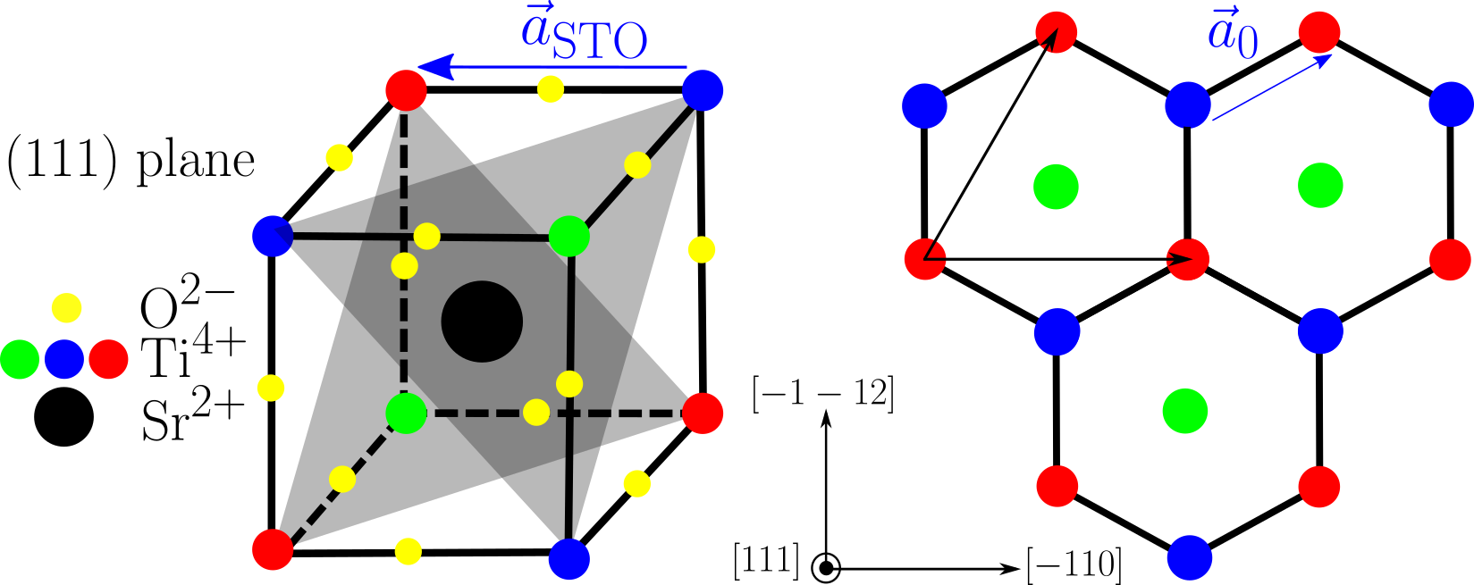
Figure 1: STO side, just below the (111) LAO/STO interface, adapted from [15]. Left: cubic lattice cell the corners of which are occupied by Ti⁴⁺ ions. The gray areas indicate planes normal to the (111) direction. Right: projection onto (111) planes. Two layers of Ti⁴⁺ ions (blue and red) form a honeycomb lattice, where the two triangular sublattices are displaced by the vector $\vec{a}_{0}$. Lastly, $a_{\text{STO}}=3.905\text{\AA}$ and $a_{0}=\sqrt{2/3}a_{\text{STO}}$.

The two-dimensional electron gas (2DEG) is located on the STO side of the LAO/STO interface [12]. From a structural point of view, the three-dimensional (3D) SrTiO₃ crystal has a ABO₃ cubic perovskite structure (left panel, Fig. 1). In the (111) orientation, see Fig. 1, two consecutive (111) planes contain Ti ions for one and SrO₃ ionic groups for the other. Focusing on the Ti (111) planes, the atomic arrangement consists of layers of two-dimensional (2D) triangular lattices displaced by the vector $\vec{a}_{0}$ (see Fig. 1). Consequently, the Ti atoms form ABC-stacked two-dimensional 2D triangular lattices in the (111) planes (see Fig. 1, left panel). From an electronic point of view, the charge carriers hop precisely between neighboring Ti atoms through direct orbital overlap or via the O sites.

While the basic unit for the description of the 2DEG would in principle contain three (ABC) layers of Ti atoms (red, blue and green in Fig. 1), the confinement profile in the (111) direction, as seen in Ref. [12], eventually allows us to reduce the model to only two layers shown in Fig. 1 (right panel), as we have checked explicitly numerically in Appendix A. Indeed, for a unit trilayer stack, the tight-binding Hamiltonian describing the kinetics of the 2DEG parallel to the (111) interface produces nine bands (not counting spin) organized in three groups (bonding, non-bonding, anti-bonding). Numerical inspection, using representative values of hopping amplitudes, shows that the energy difference between consecutive groups is on the order of several eV such that the three non-bonding bands which come from the third (green) layer are several eVs away from the Fermi energy, as discussed in Appendix A. Additionally, the dispersions of the occupied bonding triplet bands show very little difference with those of a bilayer model, where only the first (blue) and second (red) layers are considered (see Fig. 12 of Appendix A).

We can therefore leave out the third layer and consider the system shown on the right in Fig. 1, i.e. two triangular layers (red and blue) displaced by the vector $\vec{a}_{0}$ that form a honeycomb lattice. On each site, we have the three conducting $t_{2g}$ Ti orbitals. In a first approach, we set the spin-orbit coupling (SOC) to zero and discuss its impact later in Sec. V. On a honeycomb lattice with two inequivalent sublattices, we thus have a six-band system. The orbital basis which we use to write down the tight-binding model is $\big{(}d^{1}_{yz},d^{1}_{xz},d^{1}_{xy},d^{2}_{yz},d^{2}_{xz},d^{2}_{xy}\big{)}$, where the superscript $\{1,2\}$ is the layer index, which coincides with the sublattice index when projected onto the (111) plane.

II.1 Kinetic term

The kinetic part of the model takes into account hoppings between the different lattice sites and orbitals. This term consists of hoppings only between the same orbitals that are located in different layers with amplitudes $t$ and $t_{d}$ for nearest and next nearest neighbors, respectively. The general form of the kinetic term is thus diagonal in terms of the orbitals but off-diagonal in terms of the layers. Therefore, in the $\big{(}d^{1}_{yz},d^{1}_{xz},d^{1}_{xy},d^{2}_{yz},d^{2}_{xz},d^{2}_{xy}\big{)}$ basis the kinetic term reads

$$\begin{pmatrix}0&H_{\text{cin}}\\ H_{\text{cin}}^{*}&0\end{pmatrix}=\tau_{x}\otimes\text{Re}(H_{\text{cin}})-\tau_{y}\otimes\text{Im}(H_{\text{cin}}),$$ (1)

with $H_{\text{cin}}=t\operatorname{diag}(e,f,g)$ in the basis $(d_{yz},d_{xz},d_{xy})$. The Pauli matrices $\tau_{x}$ and $\tau_{y}$ in Eq. (1) act on the layer index. Explicit expressions for the functions $e,f$ and $g$ may be found in appendix B.

II.2 Orbital mixing terms

While the kinetic term does not couple the different orbitals, such couplings are generated at the interface by orbital mixing. In appendix C, we show by symmetry considerations that a natural choice is

$$\tau_{x}\otimes H_{\text{om}}=\tau_{x}\otimes c_{0}\begin{pmatrix}0&i\delta&-i\alpha\\ -i\delta&0&i\beta\\ i\alpha&-i\beta&0\end{pmatrix},$$ (2)

where $\alpha=\sin(\sqrt{3}/2k_{x}+3/2k_{y})$, $\beta=\sin(\sqrt{3}/2k_{x}-3/2k_{y})$, $\delta=-\sin(\sqrt{3}k_{x})$ and $c_{0}$ the strength of the orbital mixing. Here, we measure the wave vectors in units of the inverse $a_{0}^{-1}$ of the distance between nearest-neighbor sites in the (111) plane (see Fig. 1), and $\tau_{x}$ is again a Pauli matrix acting on the layer degree of freedom. Note that with inversion symmetry, these terms are prohibited. But in reality, interfaces between $\text{LaAlO}_{3}$ and $\text{SrTiO}_{3}$ always have corrugation [19, 20], such that inversion symmetry is broken and orbitals that would have been orthogonal are not, resulting in non-zero overlap and allowed interorbital hoppings. It will give rise to an orbital Rashba effect.

II.3 Trigonal crystal field

Note that the (111) interface has a different point symmetry than the orbitals whose symmetry is governed by the (cubic) bulk symmetry of LAO and STO. Therefore the $t_{2g}$ orbitals are not orthogonal to each other in the hexagonal lattice, resulting in a trigonal crystal field, where the couplings have the same value because of the hexagonal symmetry. It lifts the degeneracy between the $e_{\pm g}$ orbitals and the $a_{1g}$ orbital within the conducting $t_{2g}$ orbitals of Ti. This trigonal crystal field, of strength $d$, thus couples the different orbitals in the same layers so that it may be written as

$$H_{d}=-d\tau_{0}\otimes\begin{pmatrix}0&1&1\\ 1&0&1\\ 1&1&0\end{pmatrix},$$ (3)

where $\tau_{0}$ is the identity matrix indicating that the trigonal crystal field is diagonal in the layer index.

II.4 Confinement energy

Finally, we need to take into account a confinement term that reflects the different onsite potentials for the two sublattices, which reside in different layers. It is equivalent to the Semenoff mass in graphene, breaking the $\mathcal{C}_{6}$ symmetry down to $\mathcal{C}_{3}$. We have $-VI_{3}$ for layer 1 and $VI_{3}$ for layer 2, so that this term may be written as $\tau_{z}\otimes(-VI_{3})$, in terms of the $3\times 3$ identity matrix $I_{3}$. While this term may be important for other properties of the LAO/STO interface, we will see that it does not affect those studied in this paper, and we will later omit it when reducing the six-band model to two effective three-band models that are related by particle-hole symmetry.

II.5 Six-band model

With these four terms, the six-band tight-binding model is written in the orbital basis as

$$H=\begin{pmatrix}-VI_{3}+H_{d}&H_{\text{cin}}+H_{\text{om}}\\ H_{\text{cin}}^{*}+H_{\text{om}}&VI_{3}+H_{d}\end{pmatrix}.$$ (4)

A more convenient basis is the trigonal basis in which the trigonal crystal field term is diagonal. The latter is detailed in appendix D. Hereafter, we discuss the band structure described by $H$ in the trigonal basis.

III Low-energy model

Numerical diagonalization shows that the low-filling regime occurs near the $\Gamma$ point. Moreover, in the vicinity of the latter, there are two groups of three bands separated by several eV. This is because the gap between the two groups at the $\Gamma$ point is $2(2t+t_{d})\sim 6.5$eV, and the kinetic energy is clearly the largest energy scale. Therefore, for low fillings, it appears possible to simplify the above six-band to two effective three-band models, one for each group. To make a similar structure appear explicitly in $H$, we apply the following unitary transformation

$$U=\frac{1}{\sqrt{2}}\begin{pmatrix}-1&1\\ 1&1\end{pmatrix}\otimes I_{3}$$ (5)

so that the Hamiltonian is transformed to

$$U^{\dagger}HU=\begin{pmatrix}H_{d}-H_{\text{om}}-\text{Re}(H_{\text{cin}})&-VI_{3}+i\text{Im}(H_{\text{cin}})\\ -VI_{3}-i\text{Im}(H_{\text{cin}})&H_{d}+H_{\text{om}}+\text{Re}(H_{\text{cin}})\end{pmatrix}.$$ (6)

Numerical inspection confirms that the diagonal blocks pertain to the two groups. Thus, we may focus on the lower diagonal block and take it as a low-energy three-band model that reads

$$H_{3}=H_{d}+H_{\text{om}}+\text{Re}(H_{\text{cin}}).$$ (7)

A discussion of the validity of this approximation, done in appendix E, shows that with a precision of a few meV, this three-band approximation is valid over an area centered at $\Gamma$ and covering approximately ten percent of the Brillouin zone (BZ). To be consistent with this approximation, we need to expand $H_{3}$ to quadratic order in $k$.

III.1 Quadratic three-band model

In appendix F, we show that to quadratic order, we have

$$H_{3}=-(2t+t_{d})\Big{(}1-\frac{1}{4}k^{2}\Big{)}I_{3}+\begin{pmatrix}d-t_{\text{eff}}(k_{x}^{2}-k_{y}^{2})&-2t_{\text{eff}}k_{x}k_{y}&ick_{x}\\ -2t_{\text{eff}}k_{x}k_{y}&d+t_{\text{eff}}(k_{x}^{2}-k_{y}^{2})&ick_{y}\\ -ick_{x}&-ick_{y}&-2d\end{pmatrix},$$ (8)

with $t_{\text{eff}}=(t-t_{d})/8$ and $c=3c_{0}/\sqrt{2}$. Note that $H_{3}$ is expressed in the trigonal basis (see appendix D). The trigonal crystal field lifts the threefold degeneracy at the $\Gamma$ point (between $a_{1g}$ and $e_{\pm g}$ states). The linear and quadratic terms arise from the orbital mixing and kinetic terms, respectively. $H_{3}$ can then be exactly diagonalized, and we find the following eigenvalues for the last term:

$$\epsilon_{1}=d+t_{\text{eff}}k^{2},\quad\epsilon_{2}=d+\bigg{(}\frac{c^{2}}{3d}-t_{\text{eff}}\bigg{)}k^{2},$$ (9)

and

$$\epsilon_{3}=-2d-\frac{c^{2}}{3d}k^{2},$$ (10)

to quadratic order in the wave-vector components. The values taken hereafter are those corresponding to Refs. [15, 16, 17, 12, 18], i.e. $t=1.6$ eV, $t_{d}=70$ meV, $V=100$ meV, $d=3$ meV. Additionally, we estimate $c_{0}=40$ meV. We thus find an isotropic electron-like band structure.

In the remainder of this section and in the following one, we highlight the most salient features of the quantum geometry in the low-energy limit, where analytical calculations can be readily performed and assess their impact on superconductivity. We point out that these results may apply to other (111) oxide interfaces. In Section V, we discuss the relevance of our results in an experimental context, illustrated with the LAO/STO (111) interface. The lowest energy band ($\epsilon_{3}$) is substantially flatter than the other two. Indeed, its band mass can be computed to be

$$m_{B}=\frac{\hbar^{2}}{2a_{0}^{2}}\bigg{(}\frac{2t+t_{d}}{4}-\frac{c^{2}}{3d}\bigg{)}^{-1}\simeq 21m_{0},$$ (11)

with $m_{0}\simeq 9.1\times 10^{-31}$ kg the rest mass of an electron.

Note that beyond the low-energy model, and already at the cubic level, the interorbital effects give rise to an orbital Rashba effect which moves the minimum away from the $\Gamma$ point and therefore the actual band mass differs from Eq. (11). We then plot this band structure and contrast it with the one we get from the tight-binding form of the kinetic and orbital mixing terms in Fig. 2. The band structure of the full tight-binding model in the full Brillouin Zone (BZ) is shown in Appendix G.

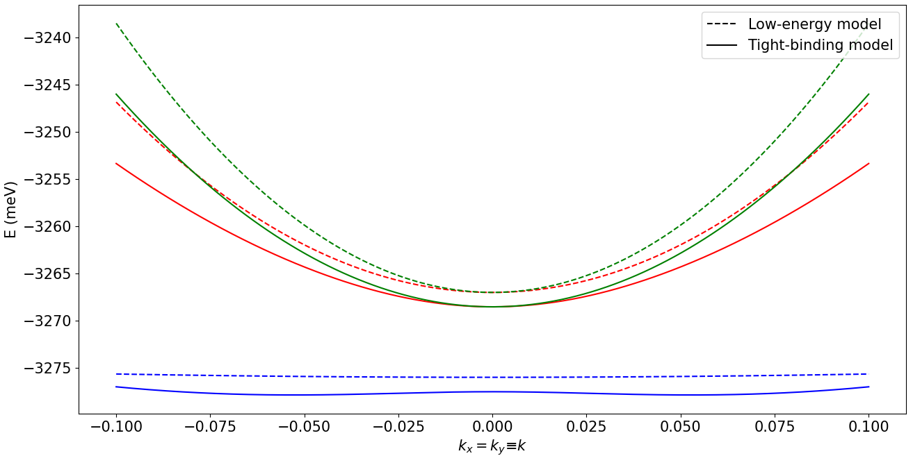
Figure 2: Energy dispersions near $\Gamma$, in the $k_{x}=k_{y}$ direction. Each color corresponds to one of the three bands, blue is the lowest band, red is the second lowest and green the third lowest band. Dashed lines correspond to the dispersions coming from the low-energy model, Eq. (8). Solid lines come from the full Tight-binding Hamiltonian, Eq. (4).

We indeed get the aforementioned precision of a few meVs. Note that the general offset of 2 meV seen in Fig. 2 is due to the confinement potential which globally shifts the bands. Such a global shift does not have a physical relevance on the quantum geometry and superfluid weight as it can be compensated by a redefinition of the chemical potential with respect to the lowest value of the lowest band. We then get a lower band that is substantially flatter than the other ones and that is close in energy to a level crossing at the $\Gamma$ point. This points to an enhanced quantum geometry, which is computed in the following section.

III.2 Quantum geometry of the lowest band

In order to compute the quantum geometry of the state with dispersion $\epsilon_{3}$, we write down the $\text{SU}(3)$ decomposition of our multiband Hamiltonian and use the formalism presented in Ref. [21]. The Hamiltonian vector form of Eq. (8) is given in appendix H.

III.2.1 Quantum metric

We begin by the quantum metric, which is defined as the real part of the quantum geometric tensor [4]

$$Q^{n}_{\mu\nu}=\bra{\partial_{\mu}n}(\mathbbm{1}-\ket{n}\bra{n})\ket{\partial_{\nu}n}=g^{n}_{\mu\nu}-\frac{i}{2}\mathcal{B}^{n}_{\mu\nu},$$ (12)

and has the physical dimension of a surface. Here, $|\partial_{\mu}n\rangle$ is the quantum state obtained by deriving the Bloch state $|n\rangle$ associated with the $n$-th band with respect to the component $k_{\mu}$ of the wave vector. Using Ref. [21], we compute the quantum metric associated with the quadratic three-band model shown in Fig. 3.

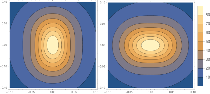
Figure 3: The quantum metric components $g_{xx}$ (left) and $g_{yy}$ (right) versus $k_{x}$ and $k_{y}$ (horizontal and vertical scales respectively), expressed in units of $a_{0}^{2}$.

The diagonal components $g_{xx}$ and $g_{yy}$ exhibit pronounced peaks at $\Gamma$, with height $g_{jj}(\Gamma)a_{0}^{-2}=c^{2}/9d^{2}\sim 90$. This feature stems from the fact that $d$ is small; in the limit $d\to 0$ the quantum metric diverges at $\Gamma$ due to the degeneracy of the energy of the three bands. Then, we have the transverse component $g_{xy}$. As seen in Fig. 4, the transverse component $g_{xy}$ is odd in $k_{x}$ and $k_{y}$. In the next section, we will see that this results in a zero transverse geometric superfluid weight. Note that, within the low-energy model, the orbital mixing terms are necessary in order to get a non-vanishing quantum metric.

Figure 4: $g_{xy}$ near $\Gamma$ versus $k_{x}$ and $k_{y}$ (horizontal and vertical scales respectively).

III.2.2 Berry curvature

We now discuss the Berry curvature. The low-energy model in Eq. (8) yields an identically zero Berry curvature. One way to obtain a non-zero Berry curvature is to add an additional term, cubic in $k$, coming from the orbital mixing. This term is a cubic orbital Rashba term, and is akin to a term obtained in Ref. [22]. Spectrally, it breaks the isotropy of the band structure, lowering the symmetry to $\mathcal{C}_{3}$ symmetry, and it splits the band minimum at $\Gamma$ into three minima located where the Berry curvature is extremal, as seen in Fig. 5. The resulting Hamiltonian vector is explicited in Appendix H, and the associated Berry curvature (for the lowest band) is plotted in Fig. 5.

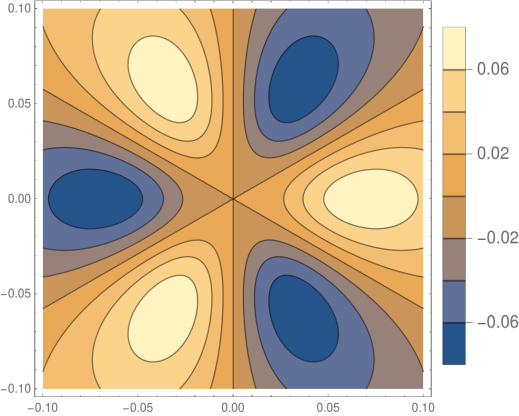
Figure 5: Berry curvature around the $\Gamma$ point, versus $k_{x}$ and $k_{y}$ (horizontal and vertical scales respectively).

Its amplitude is three orders of magnitude lower than that of the quantum metric.

The Berry curvature of the lowest band associated to the full TB model in Eq. (4) follows the same qualitative behaviour but is two orders of magnitude higher. The effect of a normal state Berry curvature on the superconducting state was discussed in Ref. [10]. It was found that, in another paradigmatic example, this Berry curvature weakens the superconducting state by lowering the magnitude of the attractive pairing interaction. However, a caveat is that, in the example studied, the normal state band geometry was isotropic, which is not the case here. Extending the approach developped in Ref. [10] to the case of an anisotropic dispersion is beyond the scope of this paper. A possible way to qualitatively assess the impact of the Berry curvature that we find in the anisotropic case would be to perform an angular averaging. But from Fig. 5 we see that this results in a zero effective Berry curvature.

IV Superfluid weight

During the past decade, a significant number of papers have discussed the role of the normal-state quantum metric on the superconducting state [6, 9, 8]. It was found that the tensor relating the supercurrent to the electrodynamic perturbation of a superconductor features two terms. One is a well-known contribution coming from the band dispersion (see Ref. [23], for example), and the other is a geometric contribution which stems from interband couplings when the normal state is described by more than just one band. In the isolated-band limit (which we consider here), this geometric contribution depends on the normal-state quantum metric [6].

Initially, this theory was developed for flat bands where the conventional contribution vanishes and the geometric contribution then dominates. While we do not have flat bands in our model, we have found one band that is significantly flatter than the other two and has a strong quantum metric. It thus seems relevant to investigate whether the normal-state quantum metric produces a sizeable effect on the superconducting state through this geometric superfluid weight. In the following section, we discuss the two contributions in the context of our low-energy model. For the superconducting state, we assume a conventional s-wave pairing, which does not seem unlikely given the disordered nature of oxide interfaces. The superconducting gap has been measured to be $\Delta=40\mu$eV in the $(001)$ LAO/STO interface [24], and a similar value for the (111) interface was reported in Ref. [25].

IV.1 BKT Temperature

In addition to the superfluid weight (which has the dimension of an energy in 2D), we consider the associated Berezinskii-Kosterlitz-Thouless (BKT) temperature, using the (isotropic) Nelson-Kosterlitz criterion [6],

$$T_{\text{BKT}}=\frac{\pi}{8k_{B}}D(T_{\text{BKT}}),$$ (13)

where $D(T)$ is the superfluid weight at temperature $T$. The BKT temperature $T_{\text{BKT}}$ is the temperature above which vortex-antivortex pairs start to unbind and thus destroy superconductivity. It is generically smaller than the critical temperature calculated within a mean-field approach. For $T_{\text{BKT}}$ not too close to $T_{c}$, we may approximate $D(T_{\text{BKT}})$ by $D(T=0)$. This defines a “mean-field” BKT temperature which is larger than the actual one and that may thus be viewed as an upper bound,

$$T_{\text{BKT}}=\frac{\pi}{8k_{B}}D(T=0).$$ (14)

IV.2 Conventional contribution

The conventional contribution to the superfluid weight at $T=0$ is given by [6, 23]

$$D_{\mu\nu,\text{conv}}=\int_{\mathscr{S}_{\text{occ}}(\mu)}\frac{d^{2}\vec{k}}{(2\pi)^{2}}\frac{\Delta^{2}}{E(\vec{k})^{3}}(\partial_{\mu}\epsilon)(\partial_{\nu}\epsilon),$$ (15)

where $\mathscr{S}_{\text{occ}}$ denotes the set of occupied states in the BZ. As discussed above, our low-energy model results in three Schrödinger-like bands. We analytically compute the conventional contribution in Appendix I and find that it is isotropic $D_{xy,\text{conv}}=0$, $D_{xx,\text{conv}}=D_{yy,\text{conv}}=D_{\text{conv}}$ with

$$D_{\text{conv}}=\frac{1}{2\pi}\Big{(}\sqrt{\Delta^{2}+\mu^{2}}-\Delta\Big{)}.$$ (16)

Fig. 6 shows a plot of $D_{\text{conv}}$ versus the chemical potential $\mu$.

Figure 6: $D_{\text{conv}}$ versus the chemical potential where we set the zero of $\mu$ at the energy $\epsilon_{3}(0)$.

IV.3 Geometric contribution

The geometric contribution at zero temperature can be written as [6]

$$D_{\mu\nu,\text{geom}}=\int_{\mathscr{S}_{\text{occ}}(\mu)}\frac{d^{2}\vec{k}}{(2\pi)^{2}}\frac{4\Delta^{2}}{E(\vec{k})}g_{\mu\nu}.$$ (17)

Note the factor of two difference with the expression given in Ref. [6]. This is because the definition of the metric there is twice the usual one [4, 21]. Again, we see that because of the parity of $g_{xy}$ we have $D_{xy,\text{geom}}=0$. Also, $D_{xx,\text{geom}}=D_{yy,\text{geom}}=D_{\text{geom}}$. If we compute $g_{xx}$ and $g_{yy}$ using the orbital (spinless) Hamiltonian, we find that $D_{\text{geom}}$ is two orders of magnitude smaller than $D_{\text{conv}}$. Notice, however, that this situation is significantly changed quantitatively, but not qualitatively, when we take into account the physical spin and SOC. In this case, discussed in detail below in Sec. V.1, we find a strongly enhanced quantum metric near the Brillouin-zone center that yields a geometric contribution to the superfluid weight that is roughly one hundred times larger than the one calculated in the absence of SOC. Due to SOC, $D_{\text{conv}}$ and $D_{\text{geom}}$ are therefore on the same order of magnitude. Anticipating the results of Sec. V.1, the SOC-corrected geometric contribution $D_{\text{geom}}$ to the superfluid weight is plotted in Fig.7 as a function of the chemical potential $\mu$.

Figure 7: $D_{\text{geom}}$ as a function of $\mu$.

The variation of the geometric contribution with the chemical potential features a dome. This can be explained by inspection of Eq. (17). Indeed, the $1/E(\vec{k})$ factor in the integral enhances the contribution at the Fermi contour, making it dominant. Focusing on this contribution, we can propose a scenario explaining the emergence of a dome in the geometric superfluid weight when the metric has a peak where the filling starts, as it is the case here. We sketch this scenario in Fig. 8.

Figure 8: Emergence of the dome of Fig.7 from the Fermi contour contribution (in red) in Eq.(17) and its corresponding location in the dome (red dot). (a) Underdoped regime. (b) Optimally doped regime. (c) Overdoped regime.

At low $\mu$, the band starts to be filled around $\Gamma$. The Fermi contour is thus at the top of the peak, but it is also narrow, such that $D_{\text{geom}}$ is low. However, as the filling increases, the Fermi contour gets wider while still being high and thus $D_{\text{geom}}$ becomes larger. This is the underdoped regime, shown in Fig. 8a. The chemical potential $\mu$ then reaches a value where the trade-off between the height and the extent of the Fermi contour is optimal, and $D_{\text{geom}}$ reaches its maximal value. This is the optimal doping in Fig. 8b. Beyond the optimal doping, the Fermi contour still gets wider but not enough to compensate the smaller values of $g_{\mu\nu}$, resulting in a decrease of $D_{\text{geom}}$. This is the overdoped regime in Fig. 8c.

V Connection to experiments

When confronting our theoretical scenario to experiments, we need to address three main issues. The first one is the extent of the difference in value of quantities obtained using the low-energy model as opposed to using the actual tight-binding model. The second issue is the link between the dome that we theoretically find when we change the chemical potential and the dome that has been experimentally observed upon variation of a gate voltage. The third issue concerns the relation between the value of $T_{\text{BKT}}$ obtained theoretically and the experimental value of the critical temperature (Sec. V.A).

V.1 Effects beyond the low-energy model

V.1.1 Rashba SOC

Our low-energy model produces isotropic constant energy contours and it features neither an atomic spin-orbit term nor a contribution from the confinement potential. We show below that it nevertheless captures the main thermodynamic characteristics of the superconducting phase in the experimentally relevant regime of small $\mu$.

If we include explicitly the spin index $\sigma=\uparrow,\downarrow$, the Bloch Hamiltonian is doubled in size and the resulting $12\times 12$ tight-binding Hamiltonian may be written in the spin-enhanced orbital basis $\big{(}d^{1}_{yz\uparrow},d^{1}_{xz\uparrow},d^{1}_{xy\uparrow},d^{2}_{yz\uparrow},d^{2}_{xz\uparrow},d^{2}_{xy\uparrow},d^{1}_{yz\downarrow},d^{1}_{xz\downarrow},d^{1}_{xy\downarrow},d^{2}_{yz\downarrow},d^{2}_{xz\downarrow},\\ d^{2}_{xy\downarrow}\big{)}$ basis. The kinetic, trigonal crystal field, orbital mixing and confinement potential parts are diagonal in spin so that their form discussed in Sec. II remains unchanged. The atomic spin-orbit Hamiltonian is diagonal in the layer index, and in each of the layers $1\;\text{or}\;2$ it reads [26]

$$\left(\begin{smallmatrix}0&i\lambda^{{}^{\prime}}&0&0&0&-\lambda^{{}^{\prime}}\\ -i\lambda^{{}^{\prime}}&0&0&0&0&i\lambda^{{}^{\prime}}\\ 0&0&0&\lambda^{{}^{\prime}}&-i\lambda^{{}^{\prime}}&0\\ 0&0&\lambda^{{}^{\prime}}&0&-i\lambda^{{}^{\prime}}&0\\ 0&0&i\lambda^{{}^{\prime}}&i\lambda^{{}^{\prime}}&0&0\\ -\lambda^{{}^{\prime}}&-i\lambda^{{}^{\prime}}&0&0&0&0\end{smallmatrix}\right)$$ (18)

where $\lambda^{{}^{\prime}}=\Delta_{SO}/3$. The spin-orbit energy $\Delta_{SO}$ is on the order of 8 meV [18].

A numerical solution of the Hamiltonian yields two groups of eigen-energies, one corresponding to bonding and the other to anti-bonding states. Their energy separation at $\Gamma$ is on the order of $3$ eV such that we only consider the lower energy bonding solutions, $E_{i,\pm}(\mathbf{k}),$ $i=1...3$, as in the case discussed before. Here, the sign $\pm$ labels the time-reversed Kramers pairs. For $\mathbf{k}=0$, $E_{+}=E_{-}$ but $E_{1}\neq E_{2}\neq E_{3}$. Close to $\Gamma$, the restriction of the Hilbert space to subspaces $1,\;2\;\text{or}\;3$ leads to spin-Rashba Hamiltonians. We may conclude that $E_{i,+}(\mathbf{k})-E_{i,-}(\mathbf{k})$ is the Rashba spin-splitting energy and that $\frac{1}{2}[E_{i,+}(\mathbf{k})+E_{i,-}(\mathbf{k})]$ is the "orbital" energy at zero spin-splitting. For the experimentally relevant regime, the chemical potential intersects the lowest energy bands $E_{1,\pm}(\mathbf{k})$. A numerical computation of the quantum geometry yields $g_{xx},\;g_{yy},\text{and}\;g_{xy}$ profiles similar to those displayed in Figs. 3 and 4 albeit with a much larger value of the peak at $\Gamma$. Similarly [7], the variations of the conventional and geometric contributions to the superfluid weight with respect to $\mu$ are similar to those shown in Figs. 6 and 7. Moreover, except for the vicinity of the $\Gamma$ point, where spin-orbit effects produce an enhanced contribution to the geometric superfluid weight, we find that the ratio between the spin-Rashba and the orbital contributions to the superfluid weight is less that $10\%$ such that the $6\times 6$ orbital Hamiltonian in Eq. (4) restricted to the lowest band triplet adequately models the low-$\mu$ experimental regime.

The $\mu$-dependence of physical quantities, such as the band filling and the conductivity, derived in the tight-binding model agree fairly well with those obtained in the low-energy model. However, the low-magnetic-field Hall resistance displays a non-monotonic behavior in the tight-binding model, caused by changes in convexity of the Fermi contour.

V.1.2 Comparing the low-energy model and the tight-binding model of Eq. (4)

We now compare the tight-binding model of Eq. (4) pertaining to the orbital part of the Hamiltonian to the low-energy model. For the band dispersions, we have already seen in Fig. 2 that the two satisfactorily agree. As for the quantum metric, there is a remarkable agreement in the direct vicinity of the $\Gamma$ point. Away from the latter we observe four additional branches, but these do not have a significant effect on the corresponding geometric superfluid weight. The latter also shows a good agreement with Fig. 7, with a dome-shaped isotropic geometric contribution, an optimal doping located at $\mu\sim 0.1$ meV and at a value close to the one depicted in Fig. 7. The low-energy model thus yields results that compare well to those obtained numerically in the model in Eq. (4).

V.1.3 Correction to $D_{\text{conv}}$ and $D_{\text{conv}}$ from thermal and disorder effects

Experimental studies of the superconducting transition in (001) and (111) oriented LAO/STO interfaces indicate that the BKT scenario is indeed relevant [25, 27, 28, 29]. The conventional superfluid weight $D_{\text{conv}}$ is proportional to the superfluid carrier density $n_{s}$. From Fig. 6, we see that $D_{\text{conv}}\sim 0.1$meV in the plotted range of chemical potential. Using the Nelson-Kosterlitz criterion, the associated BKT temperature is $T_{\text{BKT}}^{\text{conv}}\sim 500$mK, clearly larger than the reported critical temperature $T_{c}\sim 100-200$mK [27, 30, 31, 29]. This difference can be explained by thermal and disorder effects. The conventional part of the superfluid weight pertains to a superfluid density $n_{s}$ at $T=0$ K without disorder, and therefore is on the order of the carrier density. It was estimated in Ref. [32] that, because of disorder, the superfluid density only amounts to one to ten percent of the total carrier density which is of order $10^{13-14}\,\text{cm}^{-2}$. Microwave measurements of $n_{s}$ by Lesne et al. [29] similarly show a reduction of $n_{s}$ by one order of magnitude at $T_{BKT}$. Therefore, one way to take these factors into account would be applying such a renormalisation to the superfluid density and thus to the conventional superfluid weight. By contrast, $D_{\text{geom}}$ is, to our knowledge, independent of $n_{s}$.

Assessing disorder effects for (111)-oriented LAO/STO interfaces is non trivial, especially since the relative positions of the bands shift when the chemical potential varies. For a particular model, Lau et al. [33] (see their Fig. 2f) showed that the dependence of $D_{\text{geom}}$ on the disorder strength does not correlate with that of $D_{\text{conv}}$ in a clear fashion. Since a study of disorder effects on $D_{\text{geom}}$ is beyond the scope of our paper, we conservatively apply the same reduction factor, namely 90 %, to both $D_{\text{geom}}$ and $D_{\text{conv}}$. If we compute $D_{\text{geom}}$ for the orbital $6\times 6$ Hamiltonian, we find that $D_{\text{geom}}$ is always at least one order of magnitude smaller than $D_{\text{conv}}$. As mentioned previously, for the $12\times 12$ Hamiltonian, the quantum metric matrix elements are sizably enhanced near $\Gamma$ such that $D_{\text{geom}}$ and $D_{\text{conv}}$ have comparable magnitudes in the explored range of chemical potentials.

V.1.4 Total superfluid weight

Having introduced the two distinct contributions to the superfluid weight, we now discuss the total superfluid weight. We plot the corresponding BKT temperatures of Eq. (14) as a function of the chemical potential in Fig. 9 (a). The relative contributions to the superfluid weight are shown in Fig. 9b.

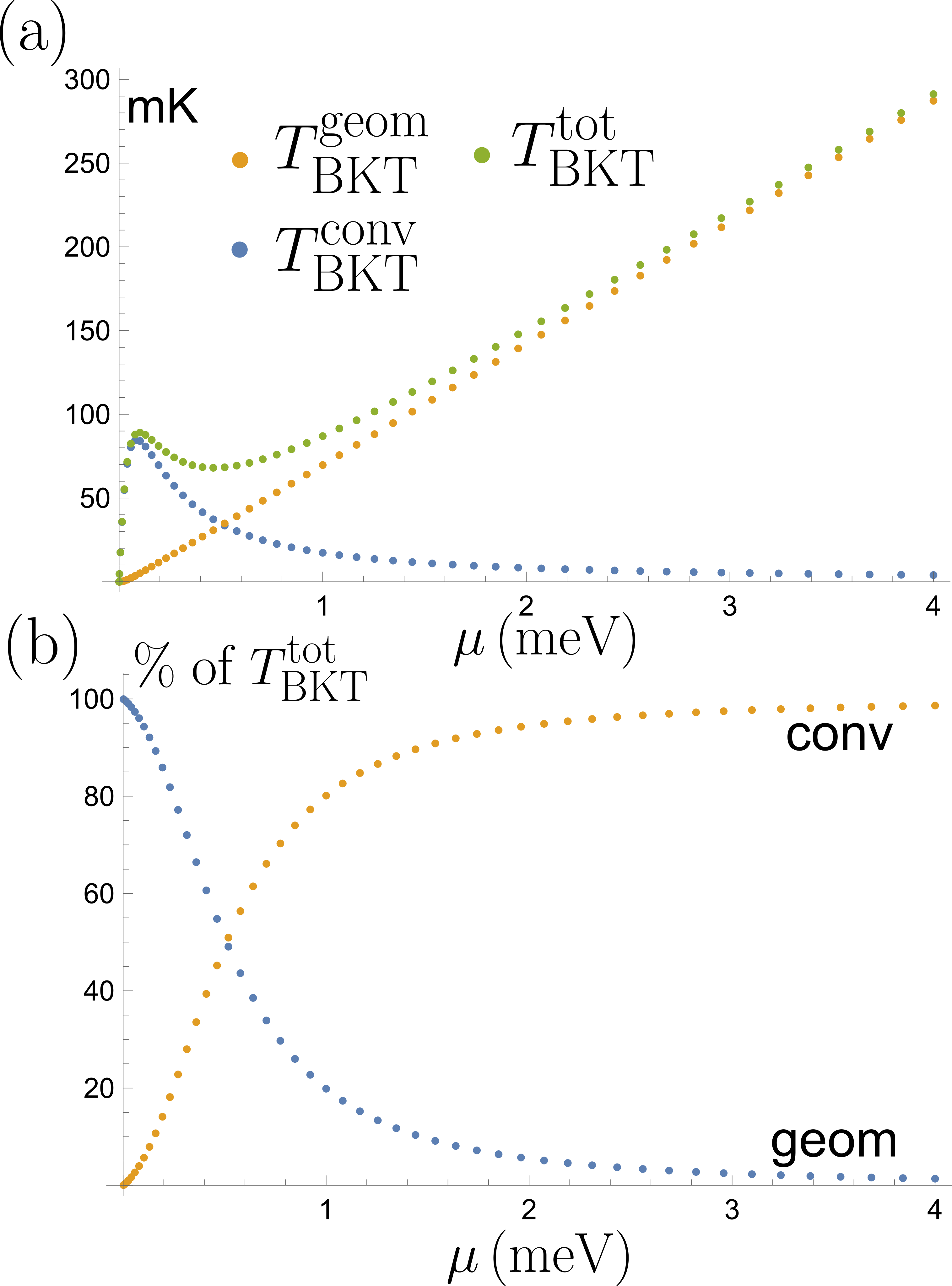
Figure 9: (a) The geometric (blue), conventional (orange) and total (green) BKT temperatures as a function of $\mu$. (b) The respective percentages of the two contributions to the total BKT temperature.

We indeed see a dome as a function of the chemical potential. At low $\mu$, the geometric contribution dominates and beyond a value $\sim 0.5$ meV the conventional contribution is largest. These are the theoretical results coming from the low-energy model given in Eq. (8). The connection to the experimental results is however more subtle due to a non-monotonic relation between gate voltage and chemical potential, as we discuss in the following subsection.

V.2 Superconducting domes

We have shown above the emergence of a superconducting dome when the chemical potential is varied. In contrast, the experimentally observed superconducting dome [30, 32, 34, 11, 31] is measured upon tuning a gate voltage $V_{g}$ or a conductivity. There are strong indications [31, 18] that the correspondence between these transport quantities and the (Hall) carrier density (or the chemical potential) is non-monotonic, possibly due to correlation effects or to the curvature of the Fermi surface. It may also be the case because of leakage of electrons out of the 2DEG into the substrate, beyond a certain gate voltage. More precisely, the Hall carrier density itself displays a dome upon changing the gate voltage indicating a non-monotonic relationship between density and gate voltage. Therefore, there is no direct correspondence between the superconducting domes that result from changing $\mu$ and the phase diagram that one obtains upon changing $V_{g}$. Based on the dependence of the Hall number on $V_{g}$, and that of $\mu$ on the carrier density, we propose that the variation of $\mu$ with $V_{g}$ is as depicted in the inset of Fig. 10, resulting in a gate voltage dependence of the critical temperature shown in Fig. 11.

Figure 10: Correspondence between the SC dome driven by a gate voltage $V_{g}$ change and the SC dome driven by a chemical potential $\mu$ change.

The scenario depicted in Fig. 10 may be understood as follows. The initial value of the chemical potential (at $V_{g}=0$) is at a point beyond 0.5 meV where the conventional contribution dominates, indicated by the point (1). At first, increasing the gate voltage also increases the chemical potential so that the BKT temperature also increases. This is the underdoped regime from point (1) to point (2). It is followed by the optimal doping region at the point (2), starting around the top of the dome. Further increase of the gate voltage leads to a decrease of the chemical potential, due to the non-monotonic relation between $V_{g}$ and $\mu$, and therefore to lower values of the BKT temperature, in the overdoped regime, from point (2) to point (3).

We can draw further conclusions from this scenario. The experimentally observed dome happens in a regime where the conventional contribution dominates and the geometric contribution should be sizeable in the overdoped regime. But if we go one step beyond and assume that further increase of the gate voltage results in an even lower value of the chemical potential, we could reach the low-$\mu$ regime and reveal the dome due to the geometric contribution. In other words, while the measured dome would be a consequence of the conventional contribution and the non-monotonicity of the chemical potential with respect to the gate voltage, there should be a secondary superconducting dome, coming from the geometric contribution, for higher values of the gate voltage. The evolution of the critical temperature (or superfluid density, BKT temperature) would be similar to that sketched in Fig. 11, as long as only the lowest energy band contributes to the superfluid condensate.

According to our picture, the two superconducting domes that one expects upon increasing the gate voltage have thus different origins. The first one is essentially (up to the optimal point) due to the non-monotonic behavior of the chemical potential with respect to the gate voltage while $T_{BKT}$ varies monotonically with $\mu$ in this interval. In contrast, the second one would be due to the “geometric” superconducting dome that is revealed when $T_{BKT}$ is plotted as a function of the chemical potential.

Figure 11: Schematic view of the proposed qualitative evolution of the BKT temperature as a function of the gate voltage. Upon increasing V_g, The underdoped and optimal doping regimes of the first dome are driven by the conventional contribution, dominating the geometric one. The overdoped regime presents a saturation, where the conventional and geometric contributions are of the same order of magnitude. The second dome comes from the geometric contribution, dominating the conventional one. Experiments that have been performed so far have only probed a small upturn part of the underdoped regime of the second dome.

VI Conclusion

Our study underscores the impact of the normal state quantum geometry on the superconducting state of the (111) $\text{LaAlO}_{3}/\text{SrTiO}_{3}$ interface. Starting from a tight-binding model, we first developed a low-energy three-band model to describe the electronic structure around the $\Gamma$ point. There, we found three Schrödinger-like bands, with one lower band being significantly flatter than the other two, which are degenerate at the $\Gamma$ point. Using a method developed in Ref. [21], we computed the quantum geometry associated to this lower band. We found that its Berry curvature is negligible in the low-energy limit. By contrast, its quantum metric presents a strong peak at the $\Gamma$ point, owing to the closeness to a degeneracy point (coming from a low value of the trigonal crystal field). Then, using a theory developed in Ref. [6], we computed the superfluid weight of this band as a function of the chemical potential $\mu$, expecting a strong geometric contribution because of the strong quantum metric. We found that this geometric contribution has a dome-shaped behavior as a function of $\mu$, and put forward a scenario explaining that the geometric contribution generically presents this dome behavior when the metric has a peak at the zero-filling point. For the conventional contribution, we analytically showed that, for a Schrödinger-like band, it has a linear behavior with respect to the chemical potential.

In the last section, we discussed subtleties regarding the relation with experimental results. We first took into account the effect of disorder by renormalizing the conventional contribution. The resulting total BKT temperature then has the form explicited in Fig. 9. The geometric contribution should dominate in a low-chemical-potential regime ($\leq 0.5$ meV). Beyond that, the conventional contribution dominates. We then discussed the relation between the dome seen as a function of the chemical potential and the ones observed experimentally as function of a gate voltage or a conductivity. Using the reported dependence of the Hall carrier density as a function of the gate voltage and our theoretical results, we put forward a scenario explaining the emergence of the observed dome. The latter would be a consequence of the non-monotonic dependence of the chemical potential on the gate voltage and would rely mostly on the conventional contribution, the geometric one being sizeable in the overdoped regime. Extrapolating this scenario, we suggest the prediction of a second superconducting dome at a higher range of gate voltage, this time ruled by the geometric contribution. Given the ubiquituousness of quantum geometry, this hidden influence on the superconducting state might be apparent in other classes of materials. Finally, this positive effect of the normal-state quantum metric on superconductivity needs to be contrasted to a previous theoretical discussion [10] suggesting a negative impact of the normal-state Berry curvature on superconductivity. This would suggest a normal state curvature-metric competition towards superconductivity.

Appendix A Bilayer model

Here, we explain in more detail the choice shown in Fig.1 to only include two layers of Ti atoms in the tight-binding (TB) model. As said in the main text, one should a priori consider three layers, so a nine band TB model (without spin). In Fig. 12 we show a comparison of the band dispersions obtained from the bilayer TB model (on the left) and a similarly obtained nine band trilayer TB model.

Figure 12: Comparison between the bilayer (left) and trilayer (right) tight-binding models.

First, we see that the bonding and anti-bonding triplets are not visibly modified by the addition of the third layer. Furthermore, the three additional bands are approximately at zero energy, and therefore several eVs away from the band we are concerned about, in the bonding triplet. Second, also the eigenstates of the bonding triplet should not be modified by the additional bands because, again, of their energy difference. Finally, from Eq.(19), we also see that following the same argument, the quantum geometric tensor [4] should not be modified by the additional bands.

$$Q^{n}_{\mu\nu}=\sum_{m\neq n}\frac{\bra{u_{n}}\partial_{\mu}H\ket{u_{m}}\bra{u_{m}}\partial_{\nu}H\ket{u_{n}}}{(E_{n}-E_{m})^{2}}.$$ (19)

In conclusion, we can reasonably discard the third layer and consider a bilayer model of Ti atoms, as shown in Fig.1.

Appendix B Expression of the kinetic terms

Hoppings are between two neighboring layers, with amplitude $t$ for $\pi$-hoppings and $t_{d}$ for $\delta$-hoppings between blue and red sites (Fig. 1). The origin of the basis lattice vectors is chosen at the center of an hexagon. $e$, $f$ and $g$ have the following expressions [35, 15],

$$\begin{cases}e=-\bigg{\{}\exp(ik_{y})+\exp[i\Big{(}\frac{\sqrt{3}}{2}k_{x}-\frac{1}{2}k_{y}\Big{)}\bigg{]}\bigg{\}}-r\exp[-i\Big{(}\frac{\sqrt{3}}{2}k_{x}+\frac{1}{2}k_{y}\Big{)}\bigg{]}\\ f=-\bigg{\{}\exp(ik_{y})+\exp[-i\Big{(}\frac{\sqrt{3}}{2}k_{x}+\frac{1}{2}k_{y}\Big{)}\bigg{]}\bigg{\}}-r\exp[i\Big{(}\frac{\sqrt{3}}{2}k_{x}-\frac{1}{2}k_{y}\Big{)}\bigg{]}\\ g=-\exp\Big(-\frac{i}{2}k_{y}\Big{missing})\times 2\cos\Big(\frac{\sqrt{3}}{2}k_{x}\Big{missing})-r\exp(ik_{y})\end{cases}\hskip 5.69054pt\text{with}\hskip 5.69054ptr=\frac{t_{d}}{t}.$$ (20)

As example, we schematize the case of the $d_{xy}$ orbitals corresponding to the hopping term $g$ in Fig. 13, and we derive $g$.

Figure 13: Diagram of the inter-layer and intra-orbital hoppings for the $d_{xy}$ orbitals. On the left, the 3D cubic lattice and the $d_{xy}$ orbitals of the Ti atoms. Hopping paths and corresponding amplitudes are shown as green color lines. On the right, the associated projection in the $(111)$ orientation.

First, consider the hopping pictured on the right of Fig. 13, going from the top red atom to the neighbouring left blue atom, with an amplitude of $t$. As seen in Fig. 13, the associated overlap in the cubic lattice is a $\pi$-overlap through the intermediate O site. The amplitude of this hopping is $t=1.6$eV. The associated phase is $\text{exp}(-i\vec{k}\cdot\vec{a}_{2})$ with $\vec{a}_{1}=(-\sqrt{3}/2,3/2)$, by equivalence with the red atom in the same motif. The similar hopping to the right also has amplitude $t$ and is associated to the phase $\text{exp}(-i\vec{k}\cdot\vec{a}_{1})$ with $\vec{a}_{1}=(\sqrt{3}/2,3/2)$. The other hopping from the top red atom to the lower blue atom is, as seen on the left of Fig. 13, the result of the direct overlap of the $d$ orbitals of the two atoms. It is therefore a $\delta$-hopping, associated with an energy amplitude $t_{d}=70$meV. As for its phase, it does not come with a phase shift, as the two atoms are part of the same motif. This way, and shifting every term by $\text{exp}(ik_{y})$ so that the origin is at the central green atom, the interlayer $d_{xy}-d_{xy}$ hopping term is given by

$$g =-te^{-i/2(-\sqrt{3}k_{x}+k_{y})}-te^{-i/2(\sqrt{3}k_{x}+k_{y})}-t_{d}e^{ik_{y}}$$

$$=-2te^{-ik_{y}/2}\cos\bigg(\frac{\sqrt{3}}{2}k_{x}\bigg{missing})-t_{d}e^{ik_{y}}.$$ (21)

Appendix C Derivation of the orbital mixing term

In the orbital basis, $H_{\text{om}}$ can be written as $A\otimes B$ with $A$ and $B$ acting in the layer and orbital subspaces respectively. The orbital mixing term consists of the interlayer and interorbital couplings so the diagonal elements of $A$ and $B$ must vanish. The hexagonal lattice structure seen in Fig. 1 has the $\mathcal{C}_{3v}$ symmetry. In order to respect the latter, we assume that all the couplings have the same magnitude in energy and that those between layer 1 to layer 2 are the same as those from layer 2 to layer 1. Therefore we can write

$$A\otimes B=c_{0}\begin{pmatrix}0&a\\ a&0\end{pmatrix}\otimes\begin{pmatrix}0&b_{1}&b_{2}\\ b_{3}&0&b_{4}\\ b_{5}&b_{6}&0\end{pmatrix},$$ (22)

where the coefficients are complex, and of modulus 1 in order to have the same magnitude $c_{0}$ in energy. They are further constrained by the fact that the term must be Hermitian. Using $(A\otimes B)^{\dagger}=A^{\dagger}\otimes B^{\dagger}$, this means that we must have $a^{*}=a$, $b_{3}=b_{1}^{*}$, $b_{5}=b_{2}^{*}$ and $b_{6}=b_{3}^{*}$. We choose $a=1$, such that

$$A\otimes B=c_{0}\tau_{x}\otimes\begin{pmatrix}0&b_{1}&b_{2}\\ b_{1}^{*}&0&b_{3}\\ b_{2}^{*}&b_{3}^{*}&0\end{pmatrix}.$$ (23)

We then introduce $(\phi_{i},\psi_{i})$ such that $b_{i}(\vec{k})=\operatorname{cos}(\phi_{i}(\vec{k}))+i\operatorname{sin}(\psi_{i}(\vec{k}))$. We look for $\phi_{i}$ and $\psi_{i}$ that are linear combinations of $k_{x}$ and $k_{y}$, which is natural for tight-binding models. These hoppings are also antisymmetric under an inversion operation $\vec{r}\longmapsto-\vec{r}$ [19], which adds the constraint $b_{i}(-\vec{k})=-b_{i}(\vec{k})$ since in $\operatorname{exp}(i\vec{k}\cdot\vec{r})$ doing $\vec{r}\longmapsto-\vec{r}$ is equivalent to $\vec{k}\longmapsto-\vec{k}$. Hence, $\operatorname{cos}(\phi_{i}(\vec{k}))=0$. Writing the allowed hoppings between the red and blue sites explicitly (Fig. 1) with the above requirements then gives $b_{i}(\vec{k})=i\operatorname{sin}(\psi_{i}(\vec{k}))=i\operatorname{sin}(\alpha_{i}k_{x}+\beta_{i}k_{y})$, with $\psi_{i}(\vec{k})=\alpha_{i}k_{x}+\beta_{i}k_{y}$. Next, the orbital mixing term needs to obey the $\mathcal{C}_{3v}$ symmetry, i.e. a $2\pi/3$ rotation with an axis perpendicular to the $(111)$ plane and a mirror symmetry parallel to the $(\overline{11}2)$ orientation. The $2\pi/3$ rotation transforms $\vec{r}=(x,y,z)$ into $\vec{r}^{\prime}=(z,x,y)$ in the original cubic unit cell. Therefore the orbitals are transformed as $(d_{yz},d_{xz},d_{xy})\longmapsto(d_{xy},d_{yz},d_{xz})$. In order to obey this $\mathcal{C}_{3}$ symmetry, we must therefore have $b_{1}(\vec{k}^{\prime})=b_{3}(\vec{k})$, $b_{2}(\vec{k}^{\prime})=b_{1}^{*}(\vec{k})$ and $b_{3}(\vec{k}^{\prime})=b_{2}^{*}(\vec{k})$ with $\vec{k}^{\prime}=(-1/2k_{x}-\sqrt{3}/2k_{y},\sqrt{3}/2k_{x}-1/2k_{y})$. The mirror operation maps $\vec{r}=(x,y,z)$ to $\vec{r}^{\prime}=(y,x,z)$ and $\vec{k}=(k_{x},k_{y})$ to $\vec{k}^{\prime}=(-k_{x},k_{y})$, so that the orbitals transform as $(d_{yz},d_{xz},d_{xy})\longmapsto(d_{xz},d_{yz},d_{xy})$. In order to obey this symmetry, we must have $b_{1}(\vec{k}^{\prime})=b_{1}^{*}(\vec{k})$, $b_{2}(\vec{k^{\prime}})=b_{3}(\vec{k})$ and $b_{3}(\vec{k}^{\prime})=b_{2}(\vec{k})$. These constraints on the $b_{i}$s put constraints on the coefficients $(\alpha_{i},\beta_{i})$ by taking the low-$k$ limit and identifying the $k_{x}$ and $k_{y}$ components (this is allowed since the constraints must be valid for all $\vec{k}$). The resulting system of equations puts five independent constraints such that $\beta_{1}=0$, $(\alpha_{2},\beta_{2})=(1/2\alpha_{1},\sqrt{3}/2\alpha_{1})$ and $(\alpha_{3},\beta_{3})=(-1/2\alpha_{1},\sqrt{3}/2\alpha_{1})$. We then recover Eq. (2) with $\alpha_{1}=-\sqrt{3}$.

Appendix D Trigonal basis

Let $U$ be the following unitary transformation in the orbital basis

$$U=\tau_{0}\otimes P,\quad P=\begin{pmatrix}-\frac{1}{\sqrt{2}}&-\frac{1}{\sqrt{6}}&\frac{1}{\sqrt{3}}\\ \frac{1}{\sqrt{2}}&-\frac{1}{\sqrt{6}}&\frac{1}{\sqrt{3}}\\ 0&\frac{2}{\sqrt{6}}&\frac{1}{\sqrt{3}}\end{pmatrix}.$$ (24)

In this basis, the trigonal crystal field becomes diagonal,

$$P^{\dagger}dH_{d}P=\begin{pmatrix}d&0&0\\ 0&d&0\\ 0&0&-2d\end{pmatrix}.$$ (25)

The first two-fold degenerate eigenvalues represent the $e_{+g}$ and $e_{-g}$ orbitals while the third one represents the $a_{1g}$ orbital. They are separated by an energy gap of $3d\simeq 10$ meV. The kinetic term is transformed as

$$H_{\text{cin}}=t\begin{pmatrix}\frac{e+f}{2}&\frac{e-f}{2\sqrt{3}}&-\frac{e-f}{\sqrt{6}}\\ \frac{e-f}{2\sqrt{3}}&\frac{e+f+4g}{6}&-\frac{e+f-2g}{3\sqrt{2}}\\ -\frac{e-f}{\sqrt{6}}&-\frac{e+f-2g}{3\sqrt{2}}&\frac{e+f+g}{3}\end{pmatrix},$$ (26)

while the orbital mixing term becomes

$$H_{\text{om}}=c_{0}\begin{pmatrix}0&iD&-iA\\ -iD&0&iB\\ iA&-iB&0\end{pmatrix},$$ (27)

with

$$\begin{cases}A=-\frac{1}{\sqrt{6}}\big{(}\alpha+\beta-2\delta\big{)}\\ B=\frac{1}{\sqrt{2}}\big{(}\alpha-\beta\big{)}\\ D=\frac{1}{\sqrt{3}}\big{(}\alpha+\beta+\delta\big{)}.\end{cases}$$ (28)

Appendix E Validity of the quadratic three-band approximation

We now discuss the validity of the three-band approximation. Doing so amounts to neglecting the off-diagonal blocks in Eq. (6) which contain the confinement energy and the imaginary part of the kinetic term. From Ref. [36], the effect of such off-diagonal terms is in $\mathcal{O}\Big{(}\frac{||E||^{2}}{\text{gap}}\Big{)}$, where $E$ is the off-diagonal perturbation. The numerically observed gap (with our choice of parameters) is around $6-7$ eV. The biggest contribution of the two terms is at zeroth and first order in $k$, i.e. in terms of scalar quantities, we have $E\sim V\pm itk$ to linear order. Therefore the intrinsic error of the three-band approximation is roughly given by

$$\frac{V^{2}+t^{2}k^{2}}{6.5\text{eV}}\simeq(1.5+400k^{2})\text{meV}.$$ (29)

This means that if we want a precision on the order of 1 meV, we find that the approximation holds until $k\sim 0.1$, so about a tenth of the BZ. This is indeed what we find when we compare the band structure with and without the off-diagonal blocks. More precisely, the confinement energy globally shifts every band by 1 to 2 meV while the imaginary part of the kinetic term breaks the isotropy of the band structure obtained within the low-energy model and gives rise to the $\mathcal{C}_{3}$ symmetric structure of ellipses seen in experimental studies (see Ref. [15] for example). So the validity of the low-energy model is restrained to the first tenth of the BZ around the $\Gamma$ point. Knowing this, what is the natural order of expansion we can do to the low-energy model ? The relevant terms will be the ones above or around our precision of a few meVs. For the orbital mixing term, the first two corrections are linear and cubic in $k$. We then have $c_{0}k\sim 4$ meV and $c_{0}k^{3}\sim 0.04$ meV for $k\sim 0.1$, so we only take the linear term. As for the kinetic term, the first two corrections are of order $tk^{2}$ and $tk^{4}$. This gives $tk^{2}\sim 10$ meV and $tk^{4}\sim 0.1$ meV, we therefore only keep the quadratic term. In conclusion, we can thus expand our three-band model to quadratic order while being coherent with the three-band approximation.

Appendix F Quadratic expansion of $H_{3}$

Here, we derive the quadratic expansion of $H_{3}$ in Eq. (8). We remind the reader that the matrices are written in the trigonal basis. For the orbital mixing term, we have

$$H_{\text{om}}=\begin{pmatrix}0&0&ick_{x}\\ 0&0&ick_{y}\\ -ick_{x}&-ick_{y}&0\end{pmatrix}+\mathcal{O}(k^{3}),$$ (30)

with $c=(3/\sqrt{2})c_{0}$. For the kinetic term, we have

$$\text{Re}(H_{\text{cin}})=-t(2+r)\bigg{(}1-\frac{1}{4}k^{2}\bigg{)}I_{3}+t\begin{pmatrix}-\frac{1}{8}(1-r)(k_{x}^{2}-k_{y}^{2})&-\frac{1}{4}(1-r)k_{x}k_{y}&\frac{1}{2\sqrt{2}}(1-r)k_{x}k_{y}\\ -\frac{1}{4}(1-r)k_{x}k_{y}&\frac{1}{8}(1-r)(k_{x}^{2}-k_{y}^{2})&\frac{1}{4\sqrt{2}}(1-r)(k_{x}^{2}-k_{y}^{2})\\ \frac{1}{2\sqrt{2}}(1-r)k_{x}k_{y}&\frac{1}{4\sqrt{2}}(1-r)(k_{x}^{2}-k_{y}^{2})&0\end{pmatrix}+\mathcal{O}(k^{4}),$$ (31)

where we separated the traceful and traceless parts using

$$\begin{pmatrix}a&0&0\\ 0&b&0\\ 0&0&c\end{pmatrix}=\frac{a+b+c}{3}I_{3}+\frac{a-b}{2}\lambda_{3}+\frac{a+b-2c}{2\sqrt{3}}\lambda_{8},$$ (32)

in terms of the Gell-Mann matrices. Now, if we define $t_{\text{eff}}=(t-t_{d})/8$, we indeed find Eq. (8), neglecting the quadratic terms whenever there already exists a linear term.

Appendix G Band structure of Eq. (4)

Figure 14: Lower triplet of the tight-binding model in Eq. (4). (a) Lowest band in the full BZ. (b) Second lowest band in the full BZ. (c) Third lowest band in the full BZ.

An important issue for our discussion here, from the electronic point of view, is the absence of other electron or hole pockets in the first BZ that would provide other and possibly different metallic and superconducting properties of the system. We therefore plot the dispersion of the lowest three bands in the entire BZ (see Fig. 14), where we clearly see that the band minima are situated at the $\Gamma$ point and that there are no other pockets in the BZ for our range of chemical potential.

Appendix H Hamiltonian vector

The Hamiltonian vector of $H_{3}$ at quadratic order is given by

$$\vec{h}=\left(-2t_{\text{eff}}k_{x}k_{y},-t_{\text{eff}}\big{(}k_{x}^{2}-k_{y}^{2}\big{)},0,-ck_{x},0,-ck_{y},\sqrt{3}d\right).$$ (33)

We then have $H_{3}=\vec{h}\cdot\vec{\lambda}$ in terms of the vector $\vec{\lambda}$ regrouping the eight Gell-Mann matrices, where we have omitted the traceful term which is irrelevant in the calculation of the quantum geometry [21]. As said in the corresponding subsection, we find an identically zero Berry curvature. To have a non-zero Berry curvature one way is to add a cubic term coming from the orbital mixing term, which breaks the isotropy of the problem and rather has a $\mathcal{C}_{3}$ symmetry. The Hamiltonian vector $\vec{h}$ then becomes

$$\vec{h}=\left(-2t_{\text{eff}}k_{x}k_{y},-\frac{1}{4\sqrt{2}}ck_{x}\big{(}k_{x}^{2}-3k_{y}^{2}\big{)},-t_{\text{eff}}\big{(}k_{x}^{2}-k_{y}^{2}\big{)},0,-ck_{x},0,-ck_{y},\sqrt{3}d\right).$$ (34)

Appendix I Calculation of $D_{\text{conv}}$

Let us consider a general isotropic and quadratic band $\epsilon=\epsilon_{0}+\alpha k^{2}$. Then, we can readily show that $D^{\text{conv}}_{xx}=D^{\text{conv}}_{yy}=D_{\text{conv}}$ and $D^{\text{conv}}_{xy}=0$. We also see that $\mathscr{S}_{\text{occ}}(\mu)=B\big{(}0;\sqrt{\mu/\alpha}\big{)}$. We then have

$$D_{\text{conv}} =\frac{1}{2}\int_{\mathscr{S}_{\text{occ}}(\mu)}\frac{\Delta^{2}}{\big{[}\Delta^{2}+(\alpha k^{2}-\mu)^{2}\big{]}^{3/2}}4\alpha^{2}k^{2}\frac{d^{2}\vec{k}}{(2\pi)^{2}}$$

$$=\frac{2\alpha^{2}}{(2\pi)^{2}}\int_{0}^{2\pi}\int_{0}^{\sqrt{\mu/\alpha}}\frac{\Delta^{2}}{\big{[}\Delta^{2}+(\alpha k^{2}-\mu)^{2}\big{]}^{3/2}}k^{3}dkd\theta$$

$$=\frac{2\alpha^{2}}{2\pi}\int_{0}^{\sqrt{\mu/\alpha}}\frac{\Delta^{2}}{\big{[}\Delta^{2}+(\alpha k^{2}-\mu)^{2}\big{]}^{3/2}}k^{3}dk$$

$$=\frac{\alpha^{2}}{\pi}\frac{1}{2\alpha^{2}}\int_{0}^{\mu}\frac{\Delta^{2}}{\big{[}\Delta^{2}+(\epsilon-\mu)^{2}\big{]}^{3/2}}\epsilon d\epsilon$$

$$=\frac{1}{2\pi}\Big{(}\sqrt{\Delta^{2}+\mu^{2}}-\Delta\Big{)}.$$ (35)

References

- Bardeen et al. [1957] J. Bardeen, L. N. Cooper, and J. R. Schrieffer, Physical Review 108, 1175 (1957).
- Adams and Blount [1959] E. Adams and E. Blount, Journal of Physics and Chemistry of Solids 10, 286 (1959).
- Blount [1962] E. Blount (Academic Press, 1962) pp. 305–373.
- Berry [1989] M. V. Berry, in Geometric Phases in Physics (World Scientific, 1989).
- Peotta and Törmä [2015] S. Peotta and P. Törmä, Nature Communications 6, 8944 (2015).
- Liang et al. [2017] L. Liang, T. I. Vanhala, S. Peotta, T. Siro, A. Harju, and P. Törmä, Physical Review B 95, 024515 (2017).
- Iskin [2018] M. Iskin, Phys. Rev. A 97, 063625 (2018).
- Rossi [2021] E. Rossi, Current Opinion in Solid State and Materials Science 25, 100952 (2021).
- Törmä et al. [2022] P. Törmä, S. Peotta, and B. A. Bernevig, Nature Reviews Physics 4, 528 (2022).
- Simon et al. [2022] F. Simon, M. Gabay, M. O. Goerbig, and L. Pagot, Physical Review B 106, 214512 (2022).
- Gariglio et al. [2016] S. Gariglio, M. Gabay, and J.-M. Triscone, APL Materials 4, 060701 (2016).
- Song et al. [2018] K. Song, S. Ryu, H. Lee, T. R. Paudel, C. T. Koch, B. Park, J. K. Lee, S.-Y. Choi, Y.-M. Kim, J. C. Kim, H. Y. Jeong, M. S. Rzchowski, E. Y. Tsymbal, C.-B. Eom, and S. H. Oh, Nature Nanotechnology 13, 198 (2018).
- Doennig et al. [2013] D. Doennig, W. E. Pickett, and R. Pentcheva, Phys. Rev. Lett. 111, 126804 (2013).
- Tian et al. [2023] H. Tian, X. Gao, Y. Zhang, S. Che, T. Xu, P. Cheung, K. Watanabe, T. Taniguchi, M. Randeria, F. Zhang, C. N. Lau, and M. W. Bockrath, Nature 614, 440 (2023).
- Rödel et al. [2014] T. Rödel, C. Bareille, F. Fortuna, C. Baumier, F. Bertran, P. Le Fèvre, M. Gabay, O. Hijano Cubelos, M. Rozenberg, T. Maroutian, P. Lecoeur, and A. Santander-Syro, Physical Review Applied 1, 051002 (2014).
- De Luca et al. [2018] G. M. De Luca, R. Di Capua, E. Di Gennaro, A. Sambri, F. M. Granozio, G. Ghiringhelli, D. Betto, C. Piamonteze, N. B. Brookes, and M. Salluzzo, Physical Review B 98, 115143 (2018).
- Vivek et al. [2017] M. Vivek, M. O. Goerbig, and M. Gabay, Physical Review B 95, 10.1103/physrevb.95.165117 (2017).
- Khanna et al. [2019] U. Khanna, P. K. Rout, M. Mograbi, G. Tuvia, I. Leermakers, U. Zeitler, Y. Dagan, and M. Goldstein, Phys. Rev. Lett. 123, 036805 (2019).
- Khalsa et al. [2013] G. Khalsa, B. Lee, and A. H. MacDonald, Physical Review B 88, 041302 (2013).
- Zhong et al. [2013] Z. Zhong, A. Tóth, and K. Held, Physical Review B 87, 161102 (2013).
- Graf and Piéchon [2021] A. Graf and F. Piéchon, Physical Review B 104, 085114 (2021).
- Lesne et al. [2023] E. Lesne, Y. G. Saǧlam, R. Battilomo, M. T. Mercaldo, T. C. van Thiel, U. Filippozzi, C. Noce, M. Cuoco, G. A. Steele, C. Ortix, and A. D. Caviglia, Nature Materials 22, 576 (2023).
- Chandrasekhar and Einzel [1993] B. S. Chandrasekhar and D. Einzel, Annalen der Physik 505, 535 (1993).
- Richter et al. [2013] C. Richter, H. Boschker, W. Dietsche, E. Fillis-Tsirakis, R. Jany, F. Loder, L. F. Kourkoutis, D. A. Muller, J. R. Kirtley, C. W. Schneider, and J. Mannhart, Nature 502, 528 (2013).
- Groen [2016] I. Groen, Electronic and superconducting properties of the two-dimensional electron system at the (111) interface, https://repository.tudelft.nl (2016), Delft University of Technology, Kavli Institute of Nanoscience.
- Khalsa and MacDonald [2012] G. Khalsa and A. H. MacDonald, Phys. Rev. B 86, 125121 (2012).
- Monteiro et al. [2017] A. M. R. V. L. Monteiro, D. J. Groenendijk, I. Groen, J. de Bruijckere, R. Gaudenzi, H. S. J. van der Zant, and A. D. Caviglia, Phys. Rev. B 96, 020504 (2017).
- Manca et al. [2019] N. Manca, D. Bothner, A. M. R. V. L. Monteiro, D. Davidovikj, Y. G. Sağlam, M. Jenkins, M. Gabay, G. A. Steele, and A. D. Caviglia, Phys. Rev. Lett. 122, 036801 (2019).
- Lesne et al. [2021] E. Lesne, Y. Gozde Saglam, M. Kounalakis, M. Gabay, G. Steele, and C. Andrea, in APS March Meeting 2021, Vol. 66 (2021).
- Rout et al. [2017] P. K. Rout, E. Maniv, and Y. Dagan, Phys. Rev. Lett. 119, 237002 (2017).
- Monteiro et al. [2019] A. M. R. V. L. Monteiro, M. Vivek, D. J. Groenendijk, P. Bruneel, I. Leermakers, U. Zeitler, M. Gabay, and A. D. Caviglia, Phys. Rev. B 99, 201102 (2019).
- Bert et al. [2012] J. A. Bert, K. C. Nowack, B. Kalisky, H. Noad, J. R. Kirtley, C. Bell, H. K. Sato, M. Hosoda, Y. Hikita, H. Y. Hwang, and K. A. Moler, Physical Review B 86, 060503 (2012).
- Lau et al. [2022] A. Lau, S. Peotta, D. I. Pikulin, E. Rossi, and T. Hyart, SciPost Phys. 13, 086 (2022).
- Gariglio et al. [2015] S. Gariglio, M. Gabay, J. Mannhart, and J.-M. Triscone, Physica C: Superconductivity and its Applications 514, 189 (2015).
- Xiao et al. [2011] D. Xiao, W. Zhu, Y. Ran, N. Nagaosa, and S. Okamoto, Nature Communications 2, 596 (2011).
- Nakatsukasa [2017] Y. Nakatsukasa, in Eigenvalue Problems: Algorithms, Software and Applications in Petascale Computing, Lecture Notes in Computational Science and Engineering, edited by T. Sakurai, S.-L. Zhang, T. Imamura, Y. Yamamoto, Y. Kuramashi, and T. Hoshi (Springer International Publishing, Cham, 2017) pp. 233–249.