Inter-orbital Cooper pairing at finite energies in Rashba surface states

Abstract

Multi-band effects in hybrid structures provide a rich playground for unconventional superconductivity. We combine two complementary approaches based on density-functional theory (DFT) and effective low-energy model theory in order to investigate the proximity effect in a Rashba surface state in contact to an $s$-wave superconductor. We discuss these synergistic approaches and combine the effective model and DFT analysis at the example of a Au/Al heterostructure. This allows to predict finite-energy superconducting pairing due to the interplay of the Rashba surface state of Au, and hybridization with the electronic structure of superconducting Al. We investigate the nature of the induced superconducting pairing and quantify its mixed singlet-triplet character. Our findings demonstrate general recipes to explore real material systems that exhibit inter-orbital pairing away from the Fermi energy.

I Introduction

Materials that exhibit strong spin orbit coupling (SOC) build the foundation for a plethora of physical phenomena Manchon et al. (2015); Bihlmayer et al. (2022) with applications ranging from non-collinear topological magnetic textures (e.g. skyrmions) Fert et al. (2017) over spinorbitronics Manchon et al. (2015) or topological insulators Hasan and Kane (2010) to quantum information processing Alicea et al. (2011); Lutchyn et al. (2018); Frolov et al. (2020); Flensberg et al. (2021). Combining different materials in heterostructures not only gives rise to breaking of symmetries, which is essential to Rashba SOC Rashba (1960), but it also allows us to tailor proximity effects, where the emergent physics of the heterostructure as a whole is richer than the sum of its constituents. In the past, this has attracted a lot of interest in the context of increasing SOC in graphene Avsar et al. (2014); Gmitra and Fabian (2017); Island et al. (2019). Combining a strong-SOC material with a superconductor is, moreover, of particular use to realize topological superconductivity, that can host Majorana zero modes (MZMs). In turn, MZMs are building blocks of topological qubits Nayak et al. (2008).

In this work, we study the inter-orbital physics inherent to heterostructures consisting of superconductors and Rashba materials. In a novel way, we combine theoretical modelling of two complementary approaches that have their roots in rather disjoint communities focusing on either microscopic or mesoscopic physics. We combine the predictive power of material-specific DFT simulations with the physical insights of an analytically solvable low-energy model. The Bogoliubov-de Gennes (BdG) formalism De Gennes (1966); Zhu (2016) is the basis for both models, in particular, the DFT-based description of the superconducting state, commonly referred to as Kohn-Sham Bogoliubov-de Gennes (KS-BdG) approach Oliveira et al. (1988); Lüders et al. (2005); Csire et al. (2015); Kawamura et al. (2020); Linscheid et al. (2015). While DFT naturally accounts for multi-band effects, the effective low-energy model with a simpler treatment of only a few bands allows us to identify the symmetry of the superconducting pairing. Crystal symmetries have profound effects. For example, they may or may not cause wavefunctions to overlap, which is visible in DFT calculations. A group-theoretic analysis allows us to infer possible (unconventional) pairing channels from crystal symmetries Scheurer et al. (2017). However, group theory alone does not tell us which of the possible pairing channels really matters in a given material. Hence, only the combination of both approaches (DFT and group theory) is able to predict the emergence of experimentally relevant (unconventional) pairing channels in the laboratory.

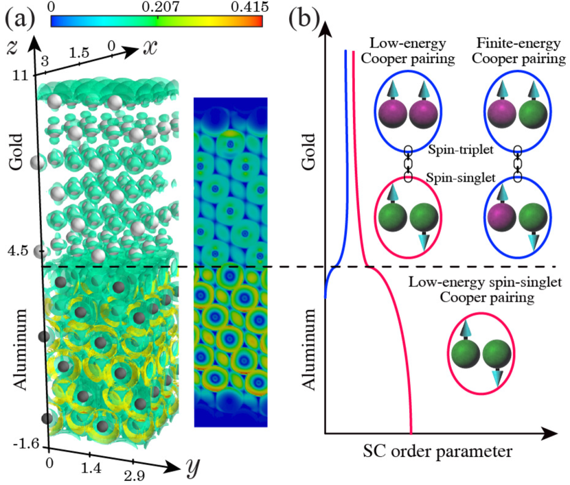
Figure 1: (a) Localization of the electron density (arb. units) around the Fermi energy throughout the Al/Au heterostructure. The background shows a cut through $x=0$. (b) Illustration of three kinds of Cooper pair tunneling and the formation of different singlet/triplet components due to the Rashba surface state. Cooper pairs formed by electrons originating from different orbitals are denoted by different colors.

Rashba SOC is intimately related to orbital mixing, often involving $p$ electrons Bihlmayer et al. (2022). Evidence for strong Rashba-SOC is found in a variety of materials ranging from heavy metal surfaces like Au or Ir and surface alloys (e.g. $\sqrt{3}\times\sqrt{3}$ Bi/Ag) LaShell et al. (1996); Varykhalov et al. (2012); Ast et al. (2007), over semiconductors like InSb Nadj-Perge et al. (2010), to topological insulators (e.g. Bi₂Se₃) King et al. (2011). We investigate the combination of such metals in hybrid structures with common superconductors, where multi-band effects are essential. In general, multi-band effects have crucial implications. They are, for instance, relevant for transport across superconductor-semiconductor interfaces in presence of Fermi surface mismatch Breunig et al. (2021), and play a major role in the superconducting diode effect Ando et al. (2020); Wu et al. (2022); Zhang et al. (2022).

As a prime example experiencing the multi-band physics of a proximitized Rashba state, we identify the interface between aluminium (Al) and gold (Au). This combination allows us to study the proximity effect with Rashba surface states. On the one hand, Al is a well-known and widely used $s$-wave superconductor whose valence band electrons are of $s-p$ orbital character. On the other hand, Au is a simple heavy metal where effects of strong SOC are particularly pronounced. In fact, as a consequence of strong SOC, the (111) surface of Au hosts a set of two spin-momentum-locked Rashba surface states LaShell et al. (1996); Nicolay et al. (2001); Henk et al. (2003, 2004); Hoesch et al. (2004); Wissing et al. (2013). Both Al and Au grow in the face centered crystal (fcc) structure and their lattice constants vary only marginally Villars and Cenzual (2016a, b). Hence, epitaxial growth of this heterostructure is feasible. It is ideally suited to gain insight into (i) hybridization of the electronic structure of Al- and Au-derived bands at the interface, (ii) proximity effect of the SOC from Au into the superconductor Al, (iii) interplay of the superconducting proximity effect and SOC in this multi-band system, and (iv) mixed singlet-triplet nature of induced superconducting pairing. The hybridized electronic structure in the Al/Au heterostructure and the emerging superconducting pairing channels due to multi-band effects are depicted in Fig. 1.

This article is structured as follows. In Sec. II, the normal state electronic structure of the Au/Al heterostructure is discussed with DFT and low-energy model approaches. In Sec. III, the DFT and model access to superconducting heterostructures are presented with emphasis on complementary insights. This modelling allows us to study the proximity effects of SOC and superconductivity in multi-band systems at the example of Al/Au interfaces. We conclude in Sec. IV, where we also comment on the feasibility of experimental detection of our predictions.

II Normal state spectrum

The DFT and model-based approaches described in this article are complementary and uniquely distinct in their methodologies. The DFT-based numerical calculations provide an ab-initio approach to the description of the electronic structure of the normal state, their scope encompasses all electronic degrees of freedom, resulting in a precise and extensive representation applicable to a broad range of materials merely from the knowledge about the crystal structure. Consequently, the intricate band structure generated by this method can be complex, comprising several bands with diverse orbital and spin character.

The effective low-energy model aims to simplify the complexity of the electronic structure by describing only a few bands, particularly those close to the $\Gamma$-point and the Fermi level. The model-based approach has the distinct advantage of deriving analytical expressions that can be applied to a wide range of material classes. Additionally, the model enables the analysis and inclusion of certain symmetries. For instance, only odd terms in $\mathbf{k}$ might appear in certain parts of the model Hamiltonian. To create a model that applies to a real material, it is, however, necessary to determine model parameters by fitting to experimental or DFT data.

II.1 Density functional theory results

Our DFT calculations for heterostructures, consisting of thin Al and Au films, are summarized in Figs. 1 and 2(a,b). Both Al and Au have a face-centered cubic (fcc) crystal structure with lattice constants of $4.08$Å and $4.05$Å, respectively Villars and Cenzual (2016a, b). We investigate an ideal interface in the close-packed (111) surface of the fcc lattice. To model the heterostructure, we use a unit cell that consists of 6 layers of Al and 6 layers of Au with the average experimental lattice constant of Al and Au, differing only by about $0.4\%$ from their respective bulk lattice constants. For our DFT calculations, we employ the full-potential relativistic Korringa-Kohn-Rostoker Green function method, as implemented in the JuKKR code The JuKKR developers (2022). This allows us to include the effect of superconductivity on the footings of the Bogoliubov-de Gennes formalism Rüßmann and Blügel (2022a). Computational details are provided in App. A.

The electronic structure of Au below the Fermi level is dominated by the fully occupied shell of $d$-electrons around $-2$ to $-8$ eV (see App. B for the corresponding DOS). In thin-film heterostructures (called “slabs”), the electrons are confined inside the slab, leading to finite-size quantization and the appearance of two-dimensional quantum-well states manifested as a series of discrete bands in the region where the bulk electronic structure is projected into the surface Brillouin zone. The presence of surfaces and interfaces, and the possible appearance of broken bonds, often leads to additional surface states or surface resonances in the electronic structure. For the Au(111) surface, Rashba surface states appear in surface projection of the bulk $L$-gap around the $\Gamma$ point of the surface Brillouin zone. They are are of $s$-$p_{z}$ orbital character LaShell et al. (1996); Henk et al. (2003).

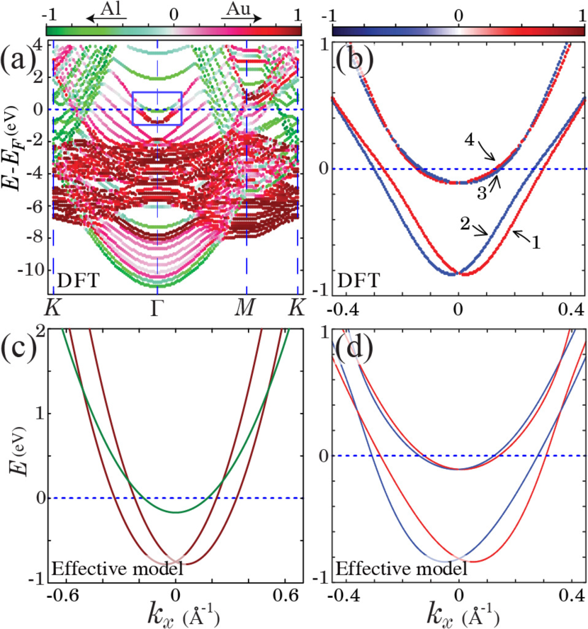
Figure 2: (a) DFT band structure for the Al/Au hybrid structure consisting of 6 layers of each element. Colorbar shows the localization of the states. (b) Enlarged view of spectrum close to the Fermi energy denoted by the blue rectangle in panel (a). Colorbar shows the spin polarization $\langle s_{y}\rangle$ (arb. units). (c) [(d)] Excitation spectrum of the normal state obtained by low-energy model Hamiltonian, given in Eq. (1), close to the Fermi energy in absence [presence] of band hybridization and including third-order Rashba spin-orbit coupling, i.e., $F_{0}=g=0$ [$F_{0}=0.2$ and $g=-8.45$]. Other model parameters are given in Tab. 1.

The region around $\Gamma$, highlighted by the blue box in Fig. 2(a), is the focus of our study. It is enlarged in Fig. 2(b). The in-plane component of the spin-polarization ($s_{y}$) perpendicular to the direction of the momentum ($k_{x}$) is shown by the color coding of the bands. Note that, due to crystal symmetries, $s_{x}$ is exactly zero in the plane through $k_{y}=0$, and $s_{z}$ is negligibly small. From the full band structure information based on DFT, we select a regime of interest for the analytical effective low-energy model. We restrict our analysis to the four states labeled 1-4, which (at small $|\mathbf{k}|$ close to $\Gamma$) are derived from the Rashba surface state of Au (states 1,2) or from Al (states 3,4), respectively. The Al states (3,4) have a quadratic dispersion and show much weaker spin-splitting. Importantly, our study reveals the existence of only a single pair of Au Rashba surface states localized at the interface of Au and vacuum. Notably, no second pair of states arises from the interface of Al and Au. This can be deduced from the localization of these states depicted in App. B. The real-space distribution of the charge density at the Fermi energy is shown in Fig. 1a. We conclude that the scattering potential at the interface is weak enough to prevent the formation of a second state at the Al/Au interface.

Aluminium is a light metal with negligible intrinsic SOC. The small SOC-induced spin-splitting seen for states 3,4 is merely a result of a proximity-induced SOC from Au to Al, hinting at sizable hybridization of the electronic structure of Al and Au. In Sec. II.2, we discuss in detail that, at higher momenta, the parabolas of the Al-derived states and the Rashba surface states intersect and hybridize, resulting in more delocalized states throughout the entire Al-Au heterostructure. This hybridization can be attributed to the compatible orbital character of the Al and Au bands, which both possess $s$-$p_{z}$ like orbital character. Ultimately, this hybridization leads to the proximity effect of the spin-orbit coupling (SOC) observed in the Al quantum well states.

II.2 Effective low-energy model

Complementary to our DFT results, we develop an effective four-band model Hamiltonian to evaluate the spectral properties of the heterostructure in an analytical manner. Guided by the insights from our DFT calculation, we construct a model for the proximitized Rashba surface state. We note a hybridization of spin-split Au surface bands and the doubly degenerate Al band near the Fermi energy. Thus, we propose the normal state model Hamiltonian to be

$$\!H_{N}\!=\!\!\sum_{\mathbf{k}}\!\left(c_{\mathbf{k},\text{Al}}^{\dagger},c_{\mathbf{k},\text{Au}}^{\dagger}\right)\!\left(\!\!\begin{array}[]{cc}\hat{h}_{\text{Al}}(\mathbf{k})&F_{0}\hat{\sigma}_{0}\\ F_{0}\hat{\sigma}_{0}&\hat{h}_{\text{Au}}(\mathbf{k})\end{array}\!\!\right)\!\left(\!\begin{array}[]{c}c_{\mathbf{k},\text{Al}}\\ c_{\mathbf{k},\text{Au}}\end{array}\!\right)\!,\!$$ (1)

where the electron annihilation operator is denoted as $c_{\mathbf{k},\nu}=(c_{\mathbf{k},\nu,s},c_{\mathbf{k},\nu,-s})^{T}$ labeled by the 2D momentum vector $\mathbf{k}=(k_{x},k_{y})$ with orbital $(\nu\in\{\text{Al},\text{Au}\})$ and spin $(s\in\{\uparrow,\downarrow\})$ degrees of freedom. $F_{0}$ signifies the hybridization strength between Al and Au bands. Furthermore, $\hat{h}_{\text{Al}(\text{Au})}(\mathbf{k})$ denotes the $2\times 2$ sector for the Al (Au) segment given by

$$\hat{h}_{\text{Al}}(\mathbf{k}) =(\alpha_{\text{Al}}k^{2}-\mu_{\text{Al}})\hat{\sigma}_{0},$$ (2)

$$\hat{h}_{\text{Au}}(\mathbf{k}) =(\alpha_{\text{Au}}k^{2}-\mu_{\text{Au}})\hat{\sigma}_{0}+\lambda(\hat{\sigma}_{x}k_{y}-k_{x}\hat{\sigma}_{y})$$

$$+g(\hat{\sigma}_{x}(k_{y}^{3}+k_{y}k_{x}^{2})-(k_{x}^{3}+k_{x}k_{y}^{2})\hat{\sigma}_{y}),$$ (3)

where $k\equiv|\mathbf{k}|=\sqrt{k_{x}^{2}+k_{y}^{2}}$; $\alpha_{\text{Al}(\text{Au})}$ and $\mu_{\text{Al}(\text{Au})}$ characterize mass term and chemical potential for Al (Au) bands, respectively. First (third) order spin-orbit coupling in the Au sector is parametrized by $\lambda$ ($g$) leading to broken inversion symmetry, i.e., $\hat{h}_{\text{Au}}(-\mathbf{k})\neq\hat{h}_{\text{Au}}(\mathbf{k})$. It is worth noting that even though the band spin-splitting of the Rashba surface state is isotropic in Au LaShell et al. (1996), it is necessary to consider higher order polynomials for the Rashba SOC in the heterostructure to match the dispersion calculated from first-principles. We attribute this observation to the reduced $C_{3v}$ point group symmetry of the interface built into the DFT model via the chosen crystal structure. We obtain the third order polynomial presented in the last term of Eq. (3) by taking the direct product of the irreducible representations of $C_{3v}$ Vajna et al. (2012). Hence, this normal-state model is constructed by intuition employing the $\mathbf{k}\cdot\mathbf{p}$ approach. This is evident in our formulation of the Hamiltonian, where we combine a Rashba model up to third order describing the Au layer with a quadratic dispersion for the Al layer and a band hybridization term $F_{0}$.

For simplicity, we focus on the 1D Brillouin zone, i.e., $\mathbf{k}=(k_{x},0)$, since our model is rotationally symmetric. Therefore, the excitation spectra of the hybrid structure become

$$E_{\mathbf{k},s}^{s^{\prime}} =\frac{1}{2}\left(\mathcal{E}_{\text{Al}}+\mathcal{E}_{\text{Au}}^{s}+s^{\prime}\sqrt{(\mathcal{E}_{\text{Al}}-\mathcal{E}_{\text{Au}}^{s})^{2}+4F_{0}^{2}}\right),$$ (4)

where $s,s^{\prime}\in\{+,-\}$. The quadratic band in the Al segment is denoted as $\mathcal{E}_{\text{Al}}=\alpha_{\text{Al}}k^{2}-\mu_{\text{Al}}$, and the spin-split band in the Au segment as $\mathcal{E}_{\text{Au}}^{\pm}=\alpha_{\text{Au}}k^{2}\pm(k\lambda+gk^{3})-\mu_{\text{Au}}$ [Fig. 2(c)]. Due to hybridization, an effective spin-orbit coupling is induced in the doubly degenerate Al bands, ultimately leading to the lifting of their degeneracy. After fitting to the DFT data, the analytical spectra given by Eq. (4) are in excellent agreement with the DFT calculation, compare Figs. 2(b) and (d).

Table 1: Values for the parameters of the low-energy model given in Eq. $\eqref{HybE}$.

	$\alpha_{i}\,(\text{eV}\cdot\text{\AA}^{2})$	$\mu_{i}\,(\text{eV})$	$F_{0}\,(\text{eV})$	$\lambda\,(\text{eV}\cdot\text{\AA})$	$g\,(\text{eV}\cdot\text{\AA}^{3})$
Al	5.6	0.17	0.2	1.1	-8.45
Au	10	0.75

III Superconducting excitation spectrum

In general, a microscopic theoretical description of the superconducting excitations can be achieved on the basis of the Bogoliubov-de Gennes (BdG) formalism De Gennes (1966); Zhu (2016), a generalization of the BCS theory of superconductivity Bardeen et al. (1957). The BdG formalism is based on the Hamiltonian

$$\hat{\mathcal{H}}_{\text{BdG}}=\left(\begin{array}[]{cc}\hat{H}_{0}&\hat{\Delta}\\ {}[\hat{\Delta}]^{\dagger}&-\hat{H}_{0}^{*}\end{array}\right),$$ (5)

where $\hat{H}_{0}$ denotes the normal state Hamiltonian and $\hat{\Delta}$ the superconducting pairing between particle and hole blocks. The BdG method is also key to the extension of DFT for superconductors Oliveira et al. (1988); Lüders et al. (2005); Csire et al. (2015); Kawamura et al. (2020); Linscheid et al. (2015), commonly referred to as Kohn-Sham Bogoliubov-de Gennes (KS-BdG) formalism. One major difference between DFT and model formulations is that Eq. (5) is formulated in real-space (DFT) or momentum space (model), if translation invariance is given.

III.1 Kohn-Sham Bogoliubov-de Gennes formalism

The central task in the superconducting DFT approach (sketched in Fig. 3) is to solve the Kohn-Sham BdG (KS-BdG) equation Oliveira et al. (1988); Suvasini et al. (1993); Csire et al. (2015)

$$H^{\mathrm{KS}}_{\mathrm{BdG}}(\mathbf{x})\Psi^{\mathrm{KS}}_{\nu}(\mathbf{x})=\varepsilon_{\nu}\Psi^{\mathrm{KS}}_{\nu}(\mathbf{x}),$$ (6)

which is a reformulation of the Schrödinger equation (or Dirac equation if relativistic effects are taken into account) in terms of an effective single particle picture. The effective single-particle wavefunctions in Nambu space $\Psi^{\mathrm{KS}}_{\nu}(\mathbf{x})=(u_{\nu}(\mathbf{x}),v_{\nu}(\mathbf{x}))^{T}$ describe, respectively, the particle and hole components at excitation energy $\varepsilon_{\nu}$ ($\nu$ is a band index labelling the electronic degrees of freedom). The KS-BdG Hamiltonian can be written in matrix form as Csire et al. (2015); Rüßmann and Blügel (2022a)

$$H^{\mathrm{KS}}_{\mathrm{BdG}}(\mathbf{x})=\left(\begin{array}[]{cc}H_{0}^{\mathrm{KS}}(\mathbf{x})-E_{\mathrm{F}}&\Delta_{\mathrm{eff}}(\mathbf{x})\\ \Delta^{*}_{\mathrm{eff}}(\mathbf{x})&E_{\mathrm{F}}-\bigl{(}H_{0}^{\mathrm{KS}}(\mathbf{x})\bigr{)}^{*},\end{array}\right)$$ (7)

where $E_{\mathrm{F}}$ is the Fermi energy. The normal state Hamiltonian

$$H^{\mathrm{KS}}_{0}(\mathbf{x})=-\nabla^{2}+V_{\mathrm{eff}}(\mathbf{x}),$$ (8)

and the effective superconducting pairing potential $\Delta_{\mathrm{eff}}$ appear in the Kohn-Sham formulation (Rydberg atomic units are used where $\hbar=1$). For $\Delta_{\mathrm{eff}}=0$, the KS-BdG equation reduces to solving the conventional Kohn-Sham equation of DFT that describes the electronic structure of the normal state.

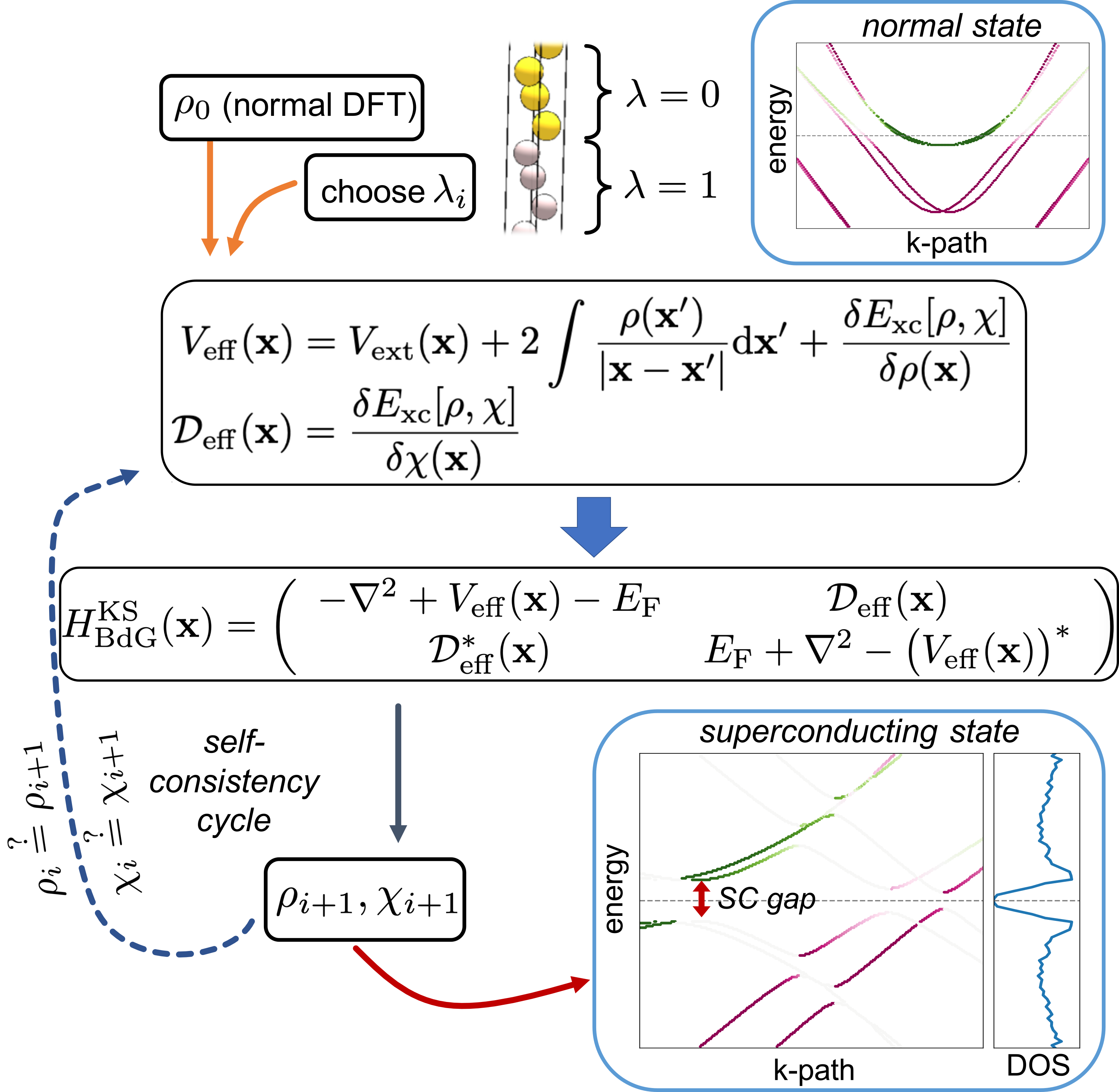
Figure 3: Schematic overview of a KS-BdG simulation that starts from the crystal structure which (in a standard DFT calculation) gives the ground state density $\rho_{0}$. For the superconducting state, the KS-BdG equations are then solved self-consistently to obtain charge and anomalous densities $\rho,\chi$ in the superconducting state which determines the superconducting band structure.

The effective single-particle potentials in Eq. (7) are functionals of the charge density $\rho(\mathbf{x})$ and the anomalous density $\chi(\mathbf{x})$ (the superconducting order parameter)Oliveira et al. (1988); Suvasini et al. (1993),

$$V_{\mathrm{eff}}(\mathbf{x}) = V_{\mathrm{ext}}(\mathbf{x})+2\int\frac{\rho(\mathbf{x}^{\prime})}{|\mathbf{x}-\mathbf{x}^{\prime}|}\mathrm{d}\mathbf{x}^{\prime}+\frac{\delta E_{\mathrm{xc}}[\rho,\chi]}{\delta\rho(\mathbf{x})},$$ (9)

$$\Delta_{\mathrm{eff}}(\mathbf{x}) = \frac{\delta E_{\mathrm{xc}}[\rho,\chi]}{\delta\chi(\mathbf{x})},$$ (10)

where functional derivatives of the exchange correlation functional $E_{\mathrm{xc}}$ appear requiring a self-consistent solution of the non-linear KS-BdG equations. The exchange correlation functional can be expressed as Suvasini et al. (1993)

$$E_{\mathrm{xc}}[\rho,\chi]=E_{\mathrm{xc}}^{0}[\rho]-\int\chi^{*}(\mathbf{x})\,\lambda\,\chi(\mathbf{x})\,\mathrm{d}\mathbf{x},$$ (11)

where the conventional exchange-correlation functional $E^{0}_{\mathrm{xc}}$ is the standard DFT term (in the normal state).

It is important to note that the above formulation of the KS-BdG equations assume a simplified form of the superconducting pairing kernel Suvasini et al. (1993) (i.e. the second term in Eq. (11)) which reduces $\lambda$ to simple constants within the cells surrounding the atoms that are however allowed to take different values throughout the computational unit cell. This assumes that the pairing interaction is local in space. This approximation was successfully used to study conventional $s$-wave superconductors Csire et al. (2015, 2016a); Saunderson et al. (2020a); Rüßmann and Blügel (2022a), heterostructures of $s$-wave superconductors and non-superconductors Csire et al. (2016b); G. Csire and J. Cserti and B. Újfalussy (2016); Rüßmann and Blügel (2022b), or impurities embedded into superconductors Saunderson et al. (2020b); Nyári et al. (2021). Hence, the effective pairing interaction takes the simple form Suvasini et al. (1993)

$$\Delta_{\mathrm{eff}}(\mathbf{x})=\lambda_{i}\chi(\mathbf{x})$$ (12)

where $\lambda_{i}$ is a set of effective coupling constants describing the intrinsic superconducting coupling that is allowed to depend on the position $i$ in the unit cell.

Finally, the charge density $\rho$ and the anomalous density $\chi$ are calculated from the particle ($u_{\nu}$) and hole components ($v_{\nu}$) of the wavefunction

$$\!\!\!\!\rho(\mathbf{x})\!\! = \!\!2\sum_{\nu}f(\varepsilon_{\nu})|u_{\nu}(\mathbf{x})|^{2}\!+\![1-\!f(\varepsilon_{\nu})]|v_{\nu}(\mathbf{x})|^{2},$$ (13)

$$\chi(\mathbf{x}) = \sum_{\nu}[1-2f(\varepsilon_{\nu})]u_{\nu}(\mathbf{x})v_{\nu}^{*}(\mathbf{x}),$$ (14)

where $f(\varepsilon)$ is the Fermi-Dirac distribution function and the summation over $\nu$ includes the full spectrum of the KS-BdG Hamiltonian.

III.2 DFT results for superconducting Al/Au

For the superconducting state, we assume that only Al has an intrinsic superconducting coupling and set the layer-dependent coupling constant in the KS-BdG calculation to

$$\lambda_{i}=\left\{\begin{array}[]{l}\lambda_{\mathrm{Al}},\quad\mathrm{if}\ i\in\mathrm{Al},\\ 0,\quad\mathrm{else},\end{array}\right.$$ (15)

where $\lambda_{\mathrm{Al}}$ is a positive real-valued constant and $i$ is an index counting the atomic layers in the Al/Au heterostructure. While the value of $\lambda_{\mathrm{Al}}$ can be regarded as a fitting parameter in this approach, we stress that only an integral quantity, leading to the overall superconducting gap size in Al, is fitted. Other spectral properties like avoided crossings and proximity effects are in fact predictions of this theory. The results of our KS-BdG simulations and analytical model for the Al/Au heterostructure are summarized in Fig. 4. For better visibility, we show results for scaled-up values of the superconducting pairing. The general trends we discuss here are, however, transferable from large to small pairing strengths with only quantitative changes. We find superconducting gaps and avoided crossings at low and finite excitation energies, labelled with $\delta$ in Fig. 4(c). These avoided crossings are rooted in the $s$-wave superconductivity induced from the Al segment included in the DFT-based simulations by $\lambda_{i}$ (the only adjustable parameter in our description of the superconducting state). The hybridization between Al and Au bands enables Cooper pair tunneling from the superconductor into the metal (see Fig. 1b). This results in a superconducting proximity effect in the Rashba surface state of Au. The large spin-splitting of the Rashba surface state allows for the pairing to have triplet character because the superconducting hybridization happens between quasiparticle bands with identical pseudo-spin degree of freedom. This will be further explained in the effective model analysis of Sec. III.3.

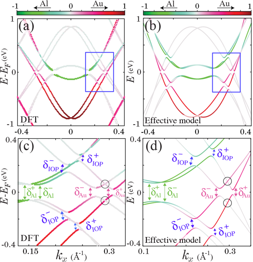
Figure 4: Superconducting band structure of the Al/Au heterostructure obtained by (a) DFT and (b) low-energy model. The red/green and grey bands indicate the particle and hole character of the BdG bands, respectively. The red/green color of the particle bands indicate the localization of the states. Panels (c) and (d) show enlarged view of the region marked by the blue box in (a) where five different superconducting avoided crossings emerge (labeled $\delta_{\mathrm{Al}}^{\pm}$, $\delta_{\mathrm{Au}}^{\pm}$, and $\delta_{\mathrm{IOP}}^{\pm}$). The absence of avoided crossings marked by black circles in (c) and (d) is due to pseudo-spin-rotational symmetry. For illustration purposes, we show results for scaled-up values of the superconducting pairing. The model parameters for the analytical model are those given in Table 1 and $\Delta=0.4F_{0}$.

The DFT calculations disclose the anisotropy of the pairing gap (see Fig. 4), which is stronger for the Rashba state at smaller momentum with $\delta^{-}_{\text{Au}}\approx 0.51\delta^{\pm}_{\text{Al}}$ and decreases to $\delta^{+}_{\text{Au}}\approx 0.38\delta^{\pm}_{\text{Al}}$ for the state at larger momentum. Furthermore, we also observe that inter-orbital pairings appear away from the Fermi energy, as indicated by $\delta_{\mathrm{IOP}}^{\pm}$, where the states with dominant Au orbital character and pseudo-spin-up intersects with the hole states with dominant Al orbital character having pseudo-spin-down degrees of freedom. This phenomenon has been referred to as inter-band pairing Moreo et al. (2009); Komendová et al. (2015); Triola and Balatsky (2017); Banerjee et al. (2018); Linder and Balatsky (2019), mirage gap Tang et al. (2021), and finite-energy Cooper pairing Bahari et al. (2022); Chakraborty and Black-Schaffer (2022); Bahari et al. (2023). However, conclusive experimental evidence supporting it is still elusive. The Al/Au hybrid structure presented here provides a simple system in which such finite-energy pairing can be observed.

Similar to the two pairing gaps $\delta_{\mathrm{Au}}^{\pm}$ in the Rashba surface state, the DFT calculation shows that the inter-orbital pairings $\delta_{\mathrm{IOP}}$ also decrease at larger momentum, i.e., $\delta_{\mathrm{IOP}}^{-}/\delta_{\mathrm{Al}}=0.60$ to $\delta_{\mathrm{IOP2}}^{+}/\delta_{\mathrm{Al}}=0.44$. Based on these observations, we pose four questions:

1. Is inter-orbital pairing exclusively the result of superconducting order or other mechanisms?

2. What determines the magnitude of the finite-energy pairing?

3. What is the magnitude of the induced spin-singlet and triplet components of the effective pairing?

4. What specific symmetries are responsible for protecting certain electron-hole band crossings that occur away from the Fermi energy?

These questions will be answered in the following sections.

III.3 Effective low-energy model for the superconducting heterostructure

Based on an effective low-energy, we can achieve a deeper understanding of the KS-BdG results. The results of our low-energy model are illustrated in Figs. 4(b) and (d). They are obtained by the model introduced in Sec. II.2. In order to obtain an analytical characterization of the superconducting pairing in the heterostructure, it is necessary to construct a BdG formalism for our minimal model, cf. Eq. $\eqref{eq:modelNormalState}$. Assuming that the superconducting pairing arises from the Al layer, we model the single-particle pairing operator as

$$H_{\Delta}=\sum_{\mathbf{k}}\left(c_{\mathbf{k},\text{Al}}^{\dagger},c_{\mathbf{k},\text{Au}}^{\dagger}\right)\left(\begin{array}[]{cc}\Delta i\hat{\sigma}_{y}&0\\ 0&0\end{array}\right)\left(\begin{array}[]{c}c_{-\mathbf{k},\text{Al}}^{\dagger}\\ c_{-\mathbf{k},\text{Au}}^{\dagger}\end{array}\right),$$ (16)

where $\Delta$ denotes the superconducting pairing strength, and the nonvanishing diagonal entry corresponds to $s$-wave spin singlet pairing in the Al layer. Since pure Au does not become a superconductor at experimentally relevant temperatures, the pairing strength in the Au layer is put to zero.

It is illuminating to represent the BdG Hamiltonian in the eigenbasis of the normal state, given in Eq. $\eqref{eq:modelNormalState}$, as defined by the $8\times 8$ matrix in Nambu space

$$\!\!\hat{H}_{\text{\text{BdG}}}\!=\!\!\left(\!\begin{array}[]{cccc}\hat{N}_{\mathbf{k}}^{++}&0&\hat{\varDelta}_{\mathbf{k}}^{++}&\hat{\varDelta}_{\mathbf{k}}^{+-}\\ 0&\hat{N}_{\mathbf{k}}^{--}&\hat{\varDelta}_{\mathbf{k}}^{-+}&\hat{\varDelta}_{\mathbf{k}}^{--}\\ {}[\hat{\varDelta}_{\mathbf{k}}^{++}]^{\dagger}&[\hat{\varDelta}_{\mathbf{k}}^{-+}]^{\dagger}&-\hat{N}_{-\mathbf{k}}^{++}&0\\ {}[\hat{\varDelta}_{\mathbf{k}}^{+-}]^{\dagger}&[\hat{\varDelta}_{\mathbf{k}}^{--}]^{\dagger}&0&-\hat{N}_{-\mathbf{k}}^{--}\end{array}\!\right)\!,$$ (17)

where the diagonal entries are the normal state dispersion relations $\hat{N}_{\mathbf{k}}^{\nu\nu}=\text{diag}(E_{\mathbf{k},+}^{\nu},E_{\mathbf{k},-}^{\nu})$ with $\nu=\pm$. Note that $E_{\mathbf{k},\pm}^{+}$ ($E_{\mathbf{k},\pm}^{-}$) refer to the upper (lower) spin-split bands which predominantly exhibit Al (Au) orbital character for small momenta, as can be seen in Fig. 2. Furthermore, the off-diagonal block in $\hat{H}_{\text{\text{BdG}}}$ is the pairing matrix projected onto the band basis (cf. App. C) as obtained by

$$\hat{\mathcal{V}}_{\mathbf{k}}^{\dagger}\text{diag}(\Delta i\hat{\sigma}_{y},0)\hat{\mathcal{V}}_{-\mathbf{k}}^{\dagger T}=\left(\begin{array}[]{cc}\hat{\varDelta}_{\mathbf{k}}^{++}&\hat{\varDelta}_{\mathbf{k}}^{+-}\\ \hat{\varDelta}_{\mathbf{k}}^{-+}&\hat{\varDelta}_{\mathbf{k}}^{--}\end{array}\right),$$ (18)

where $\hat{\mathcal{V}}_{\mathbf{k}}$ is the matrix of eigenvectors associated to the eigenvalue $\hat{\mathscr{E}}_{\mathbf{k}}$ of the normal state Hamiltonian. $\hat{\varDelta}_{\mathbf{k}}^{++}$ ($\hat{\varDelta}_{\mathbf{k}}^{--}$) correspond to the intra-band pairing matrices, specifically pairing between $E_{\mathbf{k},+}^{+}$ and $E_{\mathbf{k},-}^{+}$ ($E_{\mathbf{k},+}^{-}$ and $E_{\mathbf{k},-}^{-}$) with their hole counterparts leading to the superconducting gap for Al, i.e., $\delta_{\mathrm{Al}}$, and the proximity-induced pairing gaps labeled by ($\delta_{\mathrm{Au}}^{\pm}$) in Fig. 4. Such matrices are explicitly given by the relation

$$\hat{\varDelta}_{\mathbf{k}}^{\nu\nu}=\frac{i\Delta}{2}\left(\begin{array}[]{cc}0&1+\nu G_{\mathbf{k}}^{-}\\ -1-\nu G_{\mathbf{k}}^{+}&0\end{array}\right),$$ (19)

where $\nu=+(-)$ and

$$G_{\mathbf{k}}^{\pm}=\frac{\mathcal{E}_{\text{Al}}-\mathcal{E}_{\text{Au}}^{\pm}}{\sqrt{[\mathcal{E}_{\text{Al}}-\mathcal{E}_{\text{Au}}^{\pm}]^{2}+4F_{0}^{2}}}.$$ (20)

In Eq. $\eqref{ProjectedPairing}$, $\hat{\varDelta}_{\mathbf{k}}^{+-}$ ($\hat{\varDelta}_{\mathbf{k}}^{-+}$) indicates the inter-orbital pairing, i.e., pairing between electron bands $E_{\mathbf{k},+}^{+}$ and $E_{\mathbf{k},-}^{+}$ with hole band bands $-E_{-\mathbf{k},+}^{-}$ and $-E_{-\mathbf{k},-}^{-}$. This gives rise to the emergence of finite-energy Cooper pairing resulting in avoided crossings at finite excitation energy ($\delta_{\mathrm{IOP}}^{\pm}$) in Fig. 4 (c) and (d). The explicit form for the inter-band pairing matrix is given by

$$\hat{\varDelta}_{\mathbf{k}}^{+-}=\Delta F_{0}^{2}\left(\begin{array}[]{cc}0&\frac{-4i}{\Lambda_{\mathbf{k},1}^{-}\Lambda_{\mathbf{k},2}^{-}}\\ \frac{4i}{\Lambda_{\mathbf{k},1}^{+}\Lambda_{\mathbf{k},2}^{+}}&0\end{array}\right),$$ (21)

with

$$\Lambda_{\mathbf{k},l}^{\pm}\!=\!\sqrt{\left(\mathcal{E}_{\text{Al}}-\mathcal{E}_{\text{Au}}^{\pm}\right)^{2}\left(1+(-1)^{l}/G_{\mathbf{k}}^{\pm}\right)^{2}+4F_{0}^{2}},\!$$ (22)

where $l=\{1,2\}$. Importantly, the interplay between band hybridization and superconductivity, manifested by $\Delta F_{0}^{2}$ in Eq. $\eqref{Inter-orbitaPairing}$, intrinsically allows for the emergence of finite-energy pairing. Therefore, the inter-orbital pairing is not induced solely by superconducting order but also by band hybridization in the normal state. This is the answer to question (Q.1).

III.4 Pairing symmetry analysis

In order to determine the pairing symmetry in the hybrid structure, it is essential to establish an effective formalism that concentrates on either low or finite excitation energies. With this respect, it is necessary to derive a $4\times 4$ matrix formalism from the full $8\times 8$ BdG Hamiltonian $\hat{H}_{\text{BdG}}$. This can be done by utilizing the downfolding method specified in App. D. The downfolding method yields the effective model that enables us to investigate the superconducting properties within a given set of energy bands. As mentioned above, there are three distinct sets of spin-split bands where pairing occurs. These bands are characterized by $\nu=\nu^{\prime}=+(-)$, indicating that the pairing takes place at the Fermi energy, where the energy bands possess predominant Al (Au) orbital character. Another set of bands corresponds to the inter-orbital bands, where Al-dominated states intersect with Au-dominated hole states (and vice versa). Thus, the general form for the $4\times 4$ effective superconducting Hamiltonian becomes

$$\hat{H}_{\mathbf{k},\text{eff}}^{+\iota}=\left(\begin{array}[]{cc}\hat{N}_{\mathbf{k}}^{++}+\hat{\xi}_{1}&\hat{\varDelta}_{\mathbf{k},\text{eff}}^{+\iota}\\ {}[\hat{\varDelta}_{\mathbf{k},\text{eff}}^{+\iota}]^{\dagger}&-\hat{N}_{-\mathbf{k}}^{\iota\iota}+\hat{\xi}_{2}\end{array}\right),$$ (23)

where the diagonal entries $\hat{\xi}_{1(2)}$ are the energy shifts arsing from multiband effects given by

$$\hat{\xi}_{1} =\hat{\varDelta}_{\mathbf{k}}^{+\nu}\frac{1}{\omega+\hat{N}_{-\mathbf{k}}^{\nu\nu}}[\hat{\varDelta}_{\mathbf{k}}^{+\nu}]^{\dagger},$$ (24)

$$\hat{\xi}_{2} =\big{[}\hat{\varDelta}_{\mathbf{k}}^{-\iota}\big{]}^{\dagger}\frac{1}{\omega-\hat{N}_{\mathbf{k}}^{--}}\hat{\varDelta}_{\mathbf{k}}^{-\iota},$$ (25)

and $\omega$ is a constant. In addition, the effective pairing matrix in Eq. $\eqref{EffectiveSupHam}$ becomes

$$\!\hat{\varDelta}_{\mathbf{k},\text{eff}}^{+\iota}\!=\!\hat{\varDelta}_{\mathbf{k}}^{+\iota}+\hat{\varDelta}_{\mathbf{k}}^{+\nu}\frac{1}{\omega+\hat{N}_{-\mathbf{k}}^{\nu\nu}}[\hat{\varDelta}_{\mathbf{k}}^{-\nu}]^{\dagger}\frac{1}{\omega-\hat{N}_{\mathbf{k}}^{--}}\hat{\varDelta}_{\mathbf{k}}^{-\iota}.\!\!$$ (26)

The effective intra-(inter-)orbital superconducting Hamiltonian, i.e., $\hat{H}_{\mathbf{k},\text{eff}}^{++(+-)}$, can be obtained by setting $\iota=+(-)$ and $\nu=-(+)$. Note that $\hat{H}_{\mathbf{k},\text{eff}}^{--}$ can also be derived by substituting $(+)\leftrightarrow(-)$, and setting $\iota=-$ and $\nu=+$ in Eqs. (23-26). The spectra of the effective superconducting Hamiltonians $\hat{H}_{\mathbf{k},\text{eff}}^{++}$, $\hat{H}_{\mathbf{k},\text{eff}}^{--}$, and $\hat{H}_{\mathbf{k},\text{eff}}^{+-}$ are obtained numerically and depicted in Fig. 5(a-c). Additionally, the magnitudes of the pseudo-spin-singlet and triplet components corresponding to these spectra are illustrated in Fig. 5(d-f).

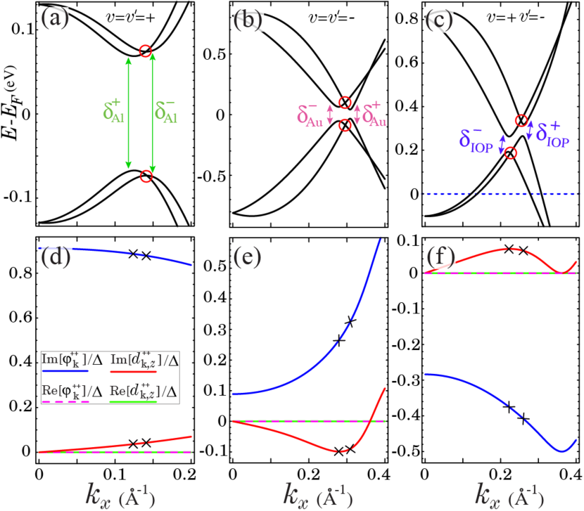
Figure 5: Effective superconducting excitation spectra for (a) $\hat{H}_{\mathbf{k},\text{eff}}^{++}$ with $\Delta=0.4F_{0}$ (b) $\hat{H}_{\mathbf{k},\text{eff}}^{--}$ with $\Delta=0.8F_{0}$, and (c) $\hat{H}_{\mathbf{k},\text{eff}}^{+-}$ with $\Delta=0.4F_{0}$. (d-f) Real and imaginary part of the pseudo-spin-singlet and pseudo-spin-triplet components of the effective pairing matrix associated with the dispersion relation illustrated in the top panels. The model parameters are the same as those given in Table 1.

Importantly, the proximity-induced intra- and inter-orbital pairing states are mixtures of singlet and triplet states due to broken inversion symmetry in the Au layer. Based on our model, only the $z$-component of the $\mathbf{d}$ vector, i.e., $\hat{\varDelta}^{+\iota}_{\mathbf{k},\text{eff}}(i\hat{\sigma}_{y})^{-1}=\varphi_{\mathbf{k}}^{+\iota}\hat{\sigma}_{0}+\mathbf{d}^{+\iota}_{\mathbf{k}}\cdot\hat{\mathbf{\sigma}}$, either at the Fermi energy or finite excitation energies is present. According to Eqs. (19) and (21), the pairing matrices are off-diagonal. Therefore, $\hat{\varDelta}_{\mathbf{k},\text{eff}}^{+\iota}$ becomes an off-diagonal matrix reflecting an effective mixed-pairing state having nonvanishing pseudo-spin-singlet $\varphi_{\mathbf{k}}^{\nu\nu}$ and pseudo-spin-triplet $d_{\mathbf{k},z}^{\nu\nu}$ character obtained as

$$\varphi_{\mathbf{k}}^{\nu\nu} =\frac{i\Delta}{4}\left[2+\nu\left(G_{\mathbf{k}}^{-}+G_{\mathbf{k}}^{+}\right)\right],$$ (27)

$$d_{\mathbf{k},z}^{\nu\nu} =\frac{i\Delta}{4}\nu\left[G_{\mathbf{k}}^{-}-G_{\mathbf{k}}^{+}\right].$$ (28)

where $\nu\in\{+,-\}$. Note that we have excluded terms proportional to the third order of $\Delta$ in Eqs. (27) and (28) as they are negligibly small in the weak pairing limit. It is worth mentioning that the property $G_{-\mathbf{k}}^{\pm}=G_{\mathbf{k}}^{\mp}$ leads to even (odd) parity for the pseudo-spin-singlet (triplet) state, i.e., $\varphi_{-\mathbf{k}}^{\nu\nu}=\varphi_{\mathbf{k}}^{\nu\nu}$ $(d_{-\mathbf{k},z}^{\nu\nu}=-d_{\mathbf{k},z}^{\nu\nu})$. The inter-orbital pairing components take the form

$$\varphi_{\mathbf{k}}^{+-} =\Delta F_{0}^{2}\left(\frac{-2i}{\Lambda_{\mathbf{k},1}^{-}\Lambda_{\mathbf{k},2}^{-}}-\frac{2i}{\Lambda_{\mathbf{k},1}^{+}\Lambda_{\mathbf{k},2}^{+}}\right),$$ (29)

$$d_{\mathbf{k},z}^{+-} =\Delta F_{0}^{2}\left(\frac{-2i}{\Lambda_{\mathbf{k},1}^{-}\Lambda_{\mathbf{k},2}^{-}}+\frac{2i}{\Lambda_{\mathbf{k},1}^{+}\Lambda_{\mathbf{k},2}^{+}}\right).$$ (30)

Overall, we observe that the pseudo-spin-singlet component is consistently larger in magnitude than the triplet component, see Fig. 5(d-f). Note that the pairing state becomes purely pseudo-spin-singlet in the absence of either band hybridization or Rashba spin-orbit coupling, i.e., when $F_{0}=0$ or $\lambda=g=0$. Therefore, the pseudo-spin-triplet component originates from the interplay between Rashba surface states and band hybridization.

The size of the avoided crossing in the spectrum of the effective pairing Hamiltonian, as expressed in Eq. (23), is given by

$$\!\!\!\delta_{\mathbf{k},\pm}^{\nu\nu^{\prime}}\!\!=\!\!\sqrt{|\varphi_{\mathbf{k}}^{\nu\nu^{\prime}}|^{2}\!+\!|d_{\mathbf{k},z}^{\nu\nu^{\prime}}|^{2}\!\pm\!|(\varphi_{\mathbf{k}}^{\nu\nu^{\prime}})^{*}d_{\mathbf{k},z}^{\nu\nu^{\prime}}\!+\!\varphi_{\mathbf{k}}^{\nu\nu^{\prime}}(d_{\mathbf{k},z}^{\nu\nu^{\prime}})^{*}|},\!$$ (31)

where the third term effectively accounts for the anisotropy observed in the magnitude of the avoided crossing, as initially demonstrated in the KS-BdG simulation in Figs. 4 and 5. This point addresses question (Q.2). Note that the Fermi surface of the hybrid structure consists of four circular rings. The inner rings are primarily composed of spin-split Al states, while they are surrounded by predominantly spin-split Au states. The superconducting hybridization happens at four Fermi momenta, i.e.,

$$\!\!\!|\mathbf{k}^{F}| \in\{k_{1}^{\text{Al}},k_{2}^{\text{Al}},k_{1}^{\text{Au}},k_{2}^{\text{Au}}\}\!$$ (32)

$$=\!\pm\!\{0.124,0.141,0.278,0.308\}\!\,\text{Å}^{-1}.\!\!\!$$ (33)

At the above momenta, we have defined the following quantities

$$\!\!\!\delta_{\mathrm{Al}}\!\equiv\!\delta_{k_{1}^{\text{Al}},+}^{++}\!\approx\!\delta_{k_{2}^{\text{Al}},-}^{++},\ \delta_{\mathrm{Au}}^{-}\!\equiv\!\delta_{k_{1}^{\text{Au}},-}^{--},\ \delta_{\mathrm{Au}}^{+}\!\equiv\!\delta_{k_{2}^{\text{Au}},+}^{--}.\!\!$$ (34)

Therefore the full pairing gap for the hybrid structure at the Fermi energy can be determined by $\delta_{\mathrm{Au}}^{+}=\text{min}(\delta_{\mathrm{Al}},\delta_{\mathrm{Au}}^{-},\delta_{\mathrm{Au}}^{+})$. The inter-orbital Cooper pairing away from the Fermi energy happens at momenta $k_{1}^{\text{IOP}}=0.221\,\text{Å}^{-1}$ and $k_{2}^{\text{IOP}}=0.26\,\text{Å}^{-1}$. Accordingly, the magnitude of finite-energy Cooper pairing is defined by $\delta_{\text{IOP}}^{-}\equiv\delta_{k_{1}^{\text{IOP}},-}^{+-}$ and $\delta_{\text{IOP}}^{+}\equiv\delta_{k_{2}^{\text{IOP}},+}^{+-}$.

The magnitudes of both intra- and inter-orbital pairings are plotted in Fig. 6(b). Apparently, the intra-orbital bands labeled by $\nu=\nu^{\prime}=+(-)$ exhibit the largest (smallest) pairing gap at low momenta, indicating a dominant Al (Au) orbital character. Interestingly, the inter-orbital pairing leads to larger avoided crossings compared to the intra-orbital pairing of predominantly Au electrons. The Fermi momenta for the intra-orbital energy bands are marked in blue and red crosses at ${k}=0.124\,\text{\AA}^{-1}$, ${k}=0.141\,\text{\AA}^{-1}$, ${k}=0.278\,\text{\AA}^{-1}$, and ${k}=0.308\,\text{\AA}^{-1}$, respectively. At these momenta, the pairing anisotropy for Al-dominated states is slightly larger than the energy bands with dominant Au orbital character. Importantly, we observe that the pairing anisotropy disappears at critical momenta ${k}_{c}=0.368\,$Å^-1, resulting in identical sizes for the pairing potentials. This occurs because the induced intra- and inter-orbital pairing becomes a purely pseudo-spin-singlet state by eliminating the spin-split nature of the bands, specifically, $d_{\mathbf{k}_{c},z}^{++}=d_{\mathbf{k}_{c},z}^{--}=d_{\mathbf{k}_{c},z}^{+-}=0$. The critical momenta can be determined by setting $\mathcal{E}_{\text{Al}}-\mathcal{E}_{\text{Au}}^{\pm}=0$ according to Eqs. (20) and (22). In general, the proximity-induced pairing exhibits a stronger presence of the pseudo-spin-singlet component over the triplet component, i.e., $d_{\mathbf{k},z}^{\nu\nu^{\prime}}/\varphi_{\mathbf{k}}^{\nu\nu^{\prime}}<1$, as illustrated in Fig. 6(a). This answers question (Q.3). Notably, among the various pairing potentials, the Au-dominated states, labeled by $\nu=\nu^{\prime}=-$, display the largest contribution from the triplet component.

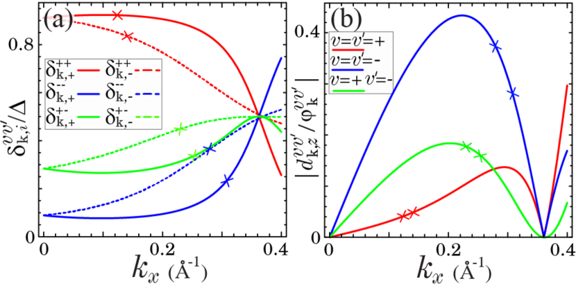
Figure 6: (a) Magnitude of the effective superconducting avoided crossings for different pairing potentials. (b) Strength of pseudo-spin-triplet $d^{\nu\nu^{\prime}}_{\mathbf{k},z}$ compared to pseudo-spin-singlet $\varphi^{\nu\nu^{\prime}}_{\mathbf{k},z}$ for the effective intra-orbital pairing potential, namely $\hat{\varDelta}_{\mathbf{k},\text{eff}}^{++}$ and $\hat{\varDelta}_{\mathbf{k},\text{eff}}^{--}$, as well as inter-orbital pairing potential $\hat{\varDelta}_{\mathbf{k},\text{eff}}^{+-}$.

III.5 Finite-energy inter-orbital avoided crossing with external magnetic fields

Note that we do not observe the occurrence of an inter-band pairing between the two dominant Rashba states displaying opposite spin-polarization marked by black and red circles in Figures 4 and 5, respectively. These crossings are protected by time-reversal and spin-rotational symmetries. They can, however, be lifted if an external Zeeman field is applied to the heterostructure. This point answers question (Q.4).

The effect of an external magnetic field on the electronic structure is shown in Fig. 7, both from DFT and low-energy model perspective. As the Zeeman field strength increases, the Rashba spin-split bands undergo further splitting.This shift of the bands leads to a decreasing superconducting energy gap in predominant Al states because spin up and spin down states are shifted away from each other. For large external magnetic fields, the gap closes completely and superconductivity is destroyed at the critical field of the superconductor. Note that the inter-band pairing between particle-hole Rashba states at finite excitation energy is clearly visible before the superconducting gap for Al states closes.

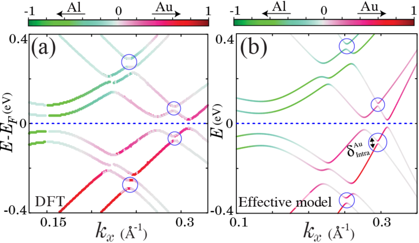
Figure 7: Superconducting band structure of Al/Au obtained by (a) DFT calculations and (b) analytical model in the presence of Zeeman magnetic field of size $B=2$ mRy. Finite-energy Cooper pairings, highlighted by blue circles, emerge due to the interplay between superconductivity and magnetic field. The colorbar indicates particle (red/green) and hole (grey) components of the BdG spectra. The model parameters for the analytical model are those given in Table 1 and $\Delta=0.4F_{0}$.

IV Discussion and Conclusion

Our results show the existence of finite-energy pairing due to the complex multi-band effects arising in the proximity effect of heterostructures between $s$-wave superconductors and heavy metals hosting Rashba surface states. The main ingredients are:

• $s$-wave superconductivity,

• surface states originating from the normal metal,

• Rashba SOC in the normal metal,

• significant hybridization between Rashba surface states and electronic structure of the $s$-wave superconductor.

If all these requirements are met finite-energy pairing emerges between discrete states of the superconductor and the Rashba surface states. This unconventional pairing leads to avoided crossings in the BdG band structures. In our case, discrete states in the superconductor are pronounced due to finite-size effects of the thin Al films. Their location relative to the position of the Au surface states can be fine-tuned by appropriate doping or film thickness. This allows us to control at which finite energy the inter-orbital pairing between Al and Au Rashba states occurs.

The size of the observable avoided crossings for the Al/Au heterostructure crucially depends on the superconducting gap of the superconductor (summarized in Tabs. A I and A II of the Appendix). Aluminium has a critical temperature of $T_{c}\approx 1\,\mathrm{T}$ and a critical magnetic field of $H_{c}\approx 10\,\mathrm{mT}$ Eisenstein (1954). In the thin film limit, both $T_{c}$ and $H_{c}$ increase substantially Meservey and Tedrow (1971); Court et al. (2008); van Weerdenburg et al. (2023), together with an increased size of the superconducting gap of $\delta_{\mathrm{Al}}\approx 300\,\mu\mathrm{eV}$  Court et al. (2008). The proximity-induced pairings at zero (within the Au Rashba bands) and finite excitation energy (due to Al-Au inter-orbital pairing) are of size $\delta_{\mathrm{IOP}}^{\pm}\approx 100-200\,\mu\mathrm{eV}$. The Au-Au inter-orbital avoided crossing that only opens up under a finite magnetic field is of size $\delta_{\mathrm{Intra}}^{\mathrm{Au}}\approx 30-50\,\mu\mathrm{eV}$ for values of the magnetic field well below the critical field of Al. These energy scales are rather small but within experimental reach. Note that energy resolutions below $10\,\mu\mathrm{eV}$ can be achieved at low temperatures Schwenk et al. (2020), see also App. F for further details.

Suitable materials engineering might further enhance the chances to detect and eventually exploit finite-energy pairings. A strong Rashba effect is typically seen in $p$-electron materials. Superconductors whose electronic structure close to the Fermi level is dominated by $sp$-electrons, as it is the case for Al, are therefore well suited to achieve strong hybridization with Rashba materials. Consequently, other superconductors with larger superconducting gaps (e.g. Pb with $T_{c}\approx 7.2\,\mathrm{K}$), that nevertheless have dominating $p$-electron character responsible for superconductivity, are promising to increase the observable size of the finite-energy pairing. Furthermore, replacing Au by the Bi/Ag(111) surface alloy, which shows a gigantic Rashba effect Ast et al. (2007), is another option for optimization. Apart from Rashba-type SOC, also bulk-inversion asymmetric crystals (e.g. BiTeI or IrBiSe Ishizaka et al. (2011); Liu et al. (2020)) where additionally Dresselhaus-type SOC-induced spin-momentum locking can be present, could be explored in this context. Observing finite-energy pairing under broken pseudo-spin-rotational symmetry benefits from a material with larger $g$-factor to increase the response to the magnetic field. InSb nanowires could be interesting systems for this purpose Aghaee et al. (2023) (Microsoft Quantum). Moreover, van der Waals heterostructures are rich material combinations where proximity effects and inter-orbital pairing can be explored Geim and Grigorieva (2013). In these systems, the possibility of engineering the band structures via Moiré superlattices provides additional knobs to tune their physical properties Andrei et al. (2021).

Albeit the abundance of heterostructures currently under investigation in the context of the search for MZMs or superconducting spintronics, multi-band physics in heterostructures remains largely unexplored. A variety of emergent phenomena can be explored in materials which show strong multi-band effects. For instance, multi-band superconductors can lead to exotic odd-frequency superconductivity Triola et al. (2020). Suitable materials engineering might further promote control over the mixed singlet-triplet character of the finite-energy pairing, that we demonstrate for Al/Au. This could be useful to control spin-triplet superconductivity, that in turn plays a pivotal role in superconducting spintronics Eschrig (2011); Linder and Robinson (2015). Moreover, spin-3/2 superconductors (e.g. YPtBi) or superconductors that show local inversion symmetry breaking in their crystal structures (e.g. CeRh₂As₂) are other examples where multi-band physics and broken symmetries inherently leads to unconventional pairing Kim et al. (2018); Khim et al. (2021). Finally, novel topological superconducting pairing at finite energies Bahari et al. (2023) is another exciting direction for future research in real materials beyond model-based calculations.

In summary, in our combined DFT and low-energy model approach we study the proximity effect in a heterostructure of Au with strong Rashba SOC and the $s$-wave superconductor Al. We show the existence of finite-energy pairing in the superconducting state and analyze the mixed singlet-triplet character of the proximity-induced pairing. Combining the strengths of predictive DFT simulations with the insights from model calculations, our results pave the way towards a deeper understanding and experimental detection of multi-band effects in superconducting heterostructures.

Appendix A Computational details of the DFT simulations

Our density functional theory calculations rely on multiple-scattering theory and employ the relativistic Korringa-Kohn-Rostoker Green function method (KKR) Ebert et al. (2011); Zabloudil et al. (2005) as implemented in the JuKKR code The JuKKR developers (2022). We use the local density approximation (LDA) to parameterize the normal state exchange correlation functional Vosko et al. (1980) and an $\ell_{\mathrm{max}}=2$ cutoff in the angular momentum expansion of the space filling Voronoi cells around the atomic centers where we make use of the exact (i.e. full-potential) description of the atomic shapes Stefanou et al. (1990); Stefanou and Zeller (1991). We use a two-dimensional geometry where periodicity is assumed in the plane, but a finite layer thickness is used in the direction along the heterostructure.

The series of DFT calculations in this study are orchestrated with the help of the AiiDA-KKR plugin Rüßmann et al. (2021a, b) to the AiiDA infrastructure Huber et al. (2020). This has the advantage that the data provenance is automatically stored in compliance to the FAIR principles of open data Wilkinson et al. (2016). The complete data set that includes the full provenance of the calculations is made publicly available in the materials cloud repository Talirz et al. (2020); Rüßmann et al. (2023).

The source codes of the AiiDA-KKR plugin Rüßmann et al. (2021b, a) and the JuKKR code The JuKKR developers (2022) are published as open source software under the MIT license at https://github.com/JuDFTteam/aiida-kkr and https://iffgit.fz-juelich.de/kkr/jukkr, respectively.

Appendix B Additional details of the normal state electronic structure from DFT

Figure A1 shows the total and layer-resolved density of states (DOS) of the Al/Au heterostructure as computed from DFT. The fully occupied $d$-shell of Au can be seen between $E-E_{F}=-8$ eV and $E-E_{F}=-2$ eV and we confirm the well-known fact that the DOS at $E_{F}$ has predominantly $s-p_{z}$ character. The electrons in aluminum show an almost, i.e. except for small van Hove singularities due to lifting of degeneracies in $sp$-bands by crystal fields, free-electron nature which can be recognized in the typical square-root shape of the DOS.

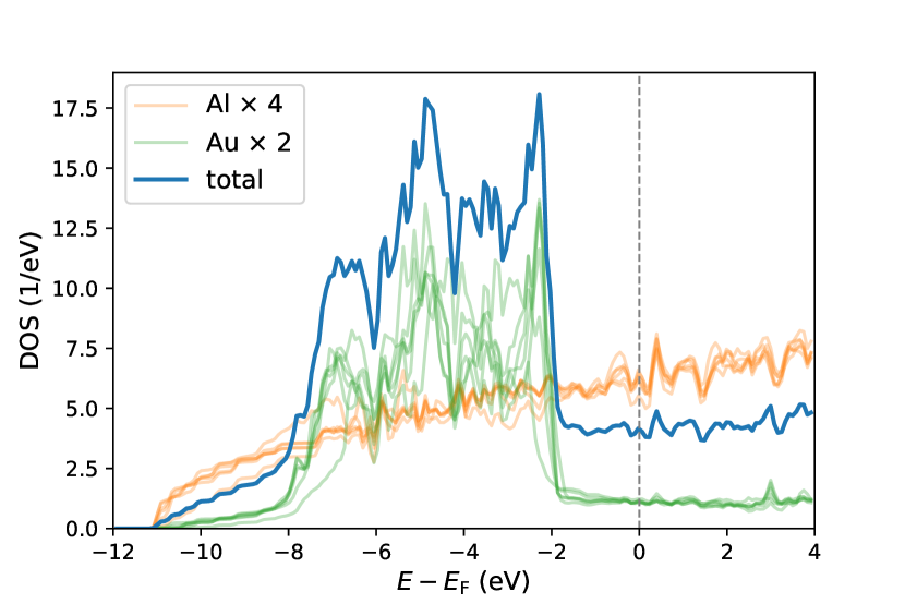
Figure A1: Density of states of the Al/Au heterostructure. The faint orange and green lines indicate the contributions of the individual Al and Au layers to the total DOS (blue line).

Figure A2 shows the wavefunction localization throughout the Al/Au heterostructure for the states labeled 1-4 in Fig. 2(b) of the main text. The wavefunction localization is shown for two values of the momentum; the top panel illustrates the situation close to $\Gamma$ at $k_{x}=0.1\,$Å^-1 where the Al and Au-derived states are clearly distinct and the bottom panel shows the situation at larger momentum of $k_{x}=0.3\,$Å^-1 where the four bands interact. At smaller momentum, the Rashba surface states (1,2) are exponentially localized at the Au-vacuum interface and have a negligible overlap with the states 3 and 4 which are delocalized throughout the Al film. In contrast, at larger momenta the four states hybridize which can be seen in the significant weight of all states in both the layers of Al and Au. This is particularly visible in comparing the top and bottom panels of Fig. A2 around layer 5 (in Al) and layer 14 (Au surface).

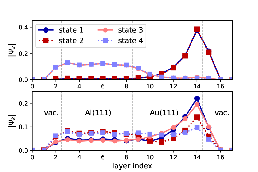
Figure A2: Wave function localization for the states 1–4 at the values of (top) $k_{x}=0.1\,$Å^-1 and (bottom) $k_{x}=0.3\,$Å^-1, which highlights the significant hybridization of the Au and Al-derived states at larger momenta.

Appendix C Band basis representation

Using the Gram–Schmidt method, we derive orthonormal eigenvectors for the normal state Hamiltonian given in Eq. (1) as

$$\!\!\!\!\!\!\!\!\hat{\mathcal{V}}(\mathbf{k}) \!\!=\!\!\!\left(\!\!\!\begin{array}[]{cccc}\frac{-i\sqrt{2}\gamma}{2\sqrt{\gamma^{2}+4F_{0}^{2}}}&\frac{i\sqrt{2}P}{2\sqrt{P^{2}+4F_{0}^{2}}}&\frac{i\sqrt{2}\upsilon}{\sqrt{\Psi^{2}+4F_{0}^{2}}}&\frac{-i\sqrt{2}\Omega}{2\sqrt{Q^{2}+4F_{0}^{2}}}\\ \frac{\sqrt{\gamma^{2}+4F_{0}^{2}}}{\sqrt{8}\Theta^{-}}&\frac{\sqrt{P^{2}+4F_{0}^{2}}}{\sqrt{8}\Theta^{+}}&\frac{-\sqrt{2}\upsilon}{\sqrt{\Psi^{2}+4F_{0}^{2}}}&\frac{-\sqrt{Q^{2}+4F_{0}^{2}}}{\sqrt{8}\Theta^{+}}\\ \frac{-i\sqrt{2}F_{0}}{\sqrt{\gamma^{2}+4F_{0}^{2}}}&\frac{i\sqrt{2}F_{0}}{\sqrt{P^{2}+4F_{0}^{2}}}&\frac{-i\sqrt{8}F_{0}}{\sqrt{\Psi^{2}+4F_{0}^{2}}}&\frac{i\sqrt{2}F_{0}}{\sqrt{Q^{2}+4F_{0}^{2}}}\\ \frac{\sqrt{2}F_{0}}{\sqrt{\gamma^{2}+4F_{0}^{2}}}&\frac{\sqrt{2}F_{0}}{\sqrt{P^{2}+4F_{0}^{2}}}&\frac{\sqrt{8}F_{0}}{\sqrt{\Psi^{2}+4F_{0}^{2}}}&\frac{\sqrt{2}F_{0}}{\sqrt{Q^{2}+4F_{0}^{2}}}\end{array}\!\!\!\right)\!,\!\!\!\!$$ (39)

where $[\hat{\mathcal{V}}(\mathbf{k})]^{\dagger}\hat{\mathcal{V}}(\mathbf{k})=1$ and we have defined

$$\Theta^{+} =\sqrt{(\Upsilon_{1}^{+})^{2}+4F_{0}^{2}}, \Theta^{-} =\sqrt{(\Upsilon_{1}^{\pm})^{2}+4F_{0}^{2}},$$ (40)

$$\Upsilon_{1}^{\pm} =\mathcal{E}_{\text{Al}}-\mathcal{E}_{\text{Au}}^{\pm}, \Upsilon_{2}^{\pm} =\mathcal{E}_{\text{Al}}+\mathcal{E}_{\text{Au}}^{\pm},$$ (41)

$$\gamma =\Theta^{-}+\Upsilon_{1}^{-}, P =\Theta^{+}+\Upsilon_{2}^{-},$$ (42)

$$\upsilon =\Theta^{-}-\Upsilon_{1}^{-}, \Psi =\Theta^{+}+\Upsilon_{1}^{+},$$ (43)

$$\Omega =\Theta^{+}-\Upsilon_{1}^{+}, Q =\Theta^{+}+\Upsilon_{1}^{+}.$$ (44)

The band basis representation for the BdG Hamiltonian can be obtained as follows. The superconducting Hamiltonian is defined by $H=\sum_{\mathbf{k}}\hat{\psi}_{\mathbf{k}}^{\dagger}\hat{\mathcal{H}}(\mathbf{k})\hat{\psi}_{\mathbf{k}}$ where the Nambu basis is $\hat{\psi}_{\mathbf{k}}=(\hat{\varphi}_{\mathbf{k}}^{\dagger},\hat{\varphi}_{-\mathbf{k}}^{\dagger T})^{T}$, and the BdG Hamiltonian is given by

$$\hat{\mathcal{H}}(\mathbf{k})=\left(\begin{array}[]{cc}\hat{H}(\mathbf{k})&\text{diag}(\Delta i\hat{\sigma}_{y},0)\\ {}[\text{diag}(\Delta i\hat{\sigma}_{y},0)]^{\dagger}&-\hat{H}^{T}(-\mathbf{k})\end{array}\right).$$ (45)

where $\hat{H}(\mathbf{k})$ is the $4\times 4$ matrix form of the normal state Hamiltonian. The band basis representation of the superconducting Hamiltonian can be obtained through the similarity transformation $\hat{H}_{\text{BdG}}(\mathbf{k})=\hat{U}^{\dagger}\hat{\mathcal{H}}(\mathbf{k})\hat{U}$ with $\hat{U}=\hat{\mathcal{V}}(\mathbf{k})\oplus[\hat{\mathcal{V}}(-\mathbf{k})]^{\dagger T}$.

Appendix D Downfolding method

In this section, we explain how to employ the downfolding method to obtain a $4\times 4$ effective Hamiltonian to describe spectral properties of the system for a specified energy window. Our starting point is a general superconducting Hamiltonian, represented in the eigenspace of the normal state given by the $8\times 8$ matrix

$$\hat{H}=\left(\begin{array}[]{cc|cc}\hat{N}_{1}&0&\hat{\varDelta}_{1}&\hat{\varDelta}_{2}\\ 0&\hat{N}_{2}&\hat{\varDelta}_{3}&\hat{\varDelta}_{4}\\ \hline\cr\hat{\varDelta}_{1}^{\dagger}&\hat{\varDelta}_{3}^{\dagger}&\hat{h}_{1}&0\\ \hat{\varDelta}_{2}^{\dagger}&\hat{\varDelta}_{4}^{\dagger}&0&\hat{h}_{2}\end{array}\right),$$ (46)

where $\hat{N}_{1(2)}$ ($\hat{h}_{1(2)}$) is a $2\times 2$ diagonal sub-block matrix containing a pair of energy bands in the normal state, and $\hat{\varDelta}_{1(4)}$ and $\hat{\varDelta}_{2(3)}$ are the pairing matrices projected onto the intra-(inter-)bands. Note that $\hat{\varDelta}_{1(4)}$ and $\hat{\varDelta}_{2(3)}$ induce full and partial pairing gaps at Fermi energy and finite excitation energies, respectively. Without loss of generality, we change the basis of $\hat{H}$ with the unitary transformation $\hat{U}$ to let the diagonal sub-blocks contain the electron-hole components with a pairing potential. This can be done with $\hat{H}^{\prime}=\hat{U}^{\dagger}\hat{H}\hat{U}$ where $\hat{U}$ is given by

$$\hat{U}^{-1} = \hat{U}^{\dagger}=\left(\begin{array}[]{cccc}1&0&0&0\\ 0&0&0&1\\ 0&1&0&0\\ 0&0&1&0\end{array}\right),$$ (51)

and $\hat{H}^{\prime}$ becomes

$$\hat{H}^{\prime}=\left(\begin{array}[]{cc|cc}\hat{N}_{1}&\hat{\varDelta}_{2}&0&\hat{\varDelta}_{1}\\ \hat{\varDelta}_{2}^{\dagger}&\hat{h}_{2}&\hat{\varDelta}_{4}^{\dagger}&0\\ \hline\cr 0&\hat{\varDelta}_{4}&\hat{N}_{2}&\hat{\varDelta}_{3}\\ \hat{\varDelta}_{1}^{\dagger}&0&\hat{\varDelta}_{3}^{\dagger}&\hat{h}_{1}\end{array}\right)\equiv\!\left(\!\!\begin{array}[]{c|c}\hat{M}_{11}&\hat{M}_{12}\\ \hline\cr\hat{M}_{21}&\hat{M}_{22}\end{array}\!\!\right)$$ (52)

In multiband systems, the downfolding method paves the way to obtain the spectral properties of a desired sub-block, e.g., $\hat{M}_{11}$, taking into account the perturbative effects of other blocks. To understand the method, we consider the eigenvalue problem for $H^{\prime}$ given by

$$\left(\!\!\begin{array}[]{cc}\hat{M}_{11}&\hat{M}_{12}\\ \hat{M}_{21}&\hat{M}_{22}\end{array}\!\!\right)\left(\begin{array}[]{c}\hat{\psi}_{A}\\ \hat{\psi}_{B}\end{array}\right) =E\left(\begin{array}[]{c}\hat{\psi}_{A}\\ \hat{\psi}_{B}\end{array}\right),$$ (59)

where $(\hat{\psi}_{A},\hat{\psi}_{B})^{T}$ is the eigenvector associated to eigenenergy $E$. Equation (59) is a coupled equation which can be written as

$$\hat{M}_{11}\hat{\psi}_{A}+\hat{M}_{12}\hat{\psi}_{B} =E\hat{\psi}_{A},$$ (60)

$$\hat{M}_{21}\hat{\psi}_{A}+\hat{M}_{22}\hat{\psi}_{B} =E\hat{\psi}_{B}.$$ (61)

Inserting $\hat{\psi}_{B}=\left(E-\hat{M}_{22}\right)^{-1}\hat{M}_{21}\hat{\psi}_{A}$ into Eq. (60) results in $\hat{M}_{11}^{\text{eff}}\hat{\psi}_{A}=E\hat{\psi}_{A}$ with

$$\hat{M}_{11}^{\text{eff}}=\hat{M}_{11}+\hat{M}_{12}\hat{\Lambda}^{-1}\hat{M}_{21},$$ (62)

where $\hat{\Lambda}=(\omega\hat{I}_{4}-\hat{M}_{22})^{-1}$, $\hat{I}_{4}$ is the $4\times 4$ identity matrix, and $\omega$ denotes a constant close to the energy range where the desired pairing happens. Thus, eigenvalues $\hat{M}_{11}^{\text{eff}}$ describes the spectral properties of $\hat{M}_{11}$ taking into account the effects of other sub-blocks. We now aim to find an expression for $\hat{\Lambda}^{-1}$. To do so, we define $\hat{\Lambda}\equiv\hat{\varepsilon}+\hat{\tilde{\Delta}}$ where $\hat{\varepsilon}$ ($\hat{\tilde{\Delta}}$) is the normal state (pairing) part given by

$$\hat{\varepsilon} =\left(\begin{array}[]{cc}\omega\hat{I}_{2}-\hat{N}_{2}&0\\ 0&\omega\hat{I}_{2}-\hat{h}_{1}\end{array}\right),$$ (65)

$$\hat{\tilde{\Delta}} =\left(\begin{array}[]{cc}0&-\hat{\varDelta}_{3}\\ -\hat{\varDelta}_{3}^{\dagger}&0\end{array}\right).$$ (68)

We can find the inverse of $\hat{\Lambda}$ using the Neumann series expansion up to second order given by

$$\!\hat{\Lambda}^{-1} \!=\hat{\varepsilon}^{-1}(\hat{I}+\hat{\tilde{\Delta}}\hat{\varepsilon}^{-1})^{-1}=\hat{\varepsilon}^{-1}\sum_{n=0}^{\infty}(-\hat{\tilde{\Delta}}\hat{\varepsilon}^{-1})^{n}$$ (69)

$$\!\approx\hat{\varepsilon}^{-1}(\hat{I}-\hat{\tilde{\Delta}}\hat{\varepsilon}^{-1})=\hat{\varepsilon}^{-1}-\hat{\varepsilon}^{-1}\hat{\tilde{\Delta}}\hat{\varepsilon}^{-1}$$ (70)

$$\!=\!\left(\!\!\begin{array}[]{cc}\!\frac{1}{\omega\hat{\sigma}_{0}-\hat{N}_{2}}&\!\frac{1}{\omega\hat{\sigma}_{0}-\hat{N}_{2}}\hat{\varDelta}_{3}\frac{1}{\omega\hat{\sigma}_{0}-\hat{h}_{1}}\\ \!\frac{1}{\omega\hat{\sigma}_{0}-\hat{h}_{1}}\big{[}\hat{\varDelta}_{3}\big{]}^{\dagger}\frac{1}{\omega\hat{\sigma}_{0}-\hat{N}_{2}}&\!\frac{1}{\omega\hat{\sigma}_{0}-\hat{h}_{1}}\end{array}\!\!\right)\!.\!\!$$ (73)

Note that Eq. (69) converges when the norm of $\hat{\tilde{\Delta}}\hat{\varepsilon}^{-1}$ is smaller than unity which can be fulfilled in the weak pairing limit. After some algebra, we arrive at an explicit relation for $\hat{M}_{11}^{\text{eff}}$ that is

$$\hat{M}_{11}^{\text{eff}}=\left(\begin{array}[]{cc}\hat{N}_{1}+\hat{\xi}_{1}&\hat{\varDelta}_{2}^{\text{eff}}\\ {}[\hat{\varDelta}_{2}^{\text{eff}}]^{\dagger}&\hat{h}_{2}+\hat{\xi}_{2}\end{array}\right),$$ (74)

where the energy shifts arising from the multiband nature as

$$\hat{\xi}_{1} =\hat{\varDelta}_{1}\frac{1}{\omega\hat{\sigma}_{0}-\hat{h}_{1}}\text{$\hat{\varDelta}_{1}^{\dagger}$},$$ (75)

$$\hat{\xi}_{2} =\hat{\varDelta}_{4}^{\dagger}\frac{1}{\omega\hat{\sigma}_{0}-\hat{N}_{2}}\hat{\varDelta}_{4}.$$ (76)

Additionally, the effective $2\times 2$ pairing matrix takes the form

$$\hat{\varDelta}_{2}^{\text{eff}}=\hat{\varDelta}_{2}+\hat{\varDelta}_{1}\frac{1}{\omega\hat{\sigma}_{0}-\hat{h}_{1}}\hat{\varDelta}_{3}^{\dagger}\frac{1}{\omega\hat{\sigma}_{0}-\hat{N}_{2}}\hat{\varDelta}_{4}.$$ (77)

According to Eqs. (16) and (24), the projected pairing matrices $\hat{\varDelta}_{1,2,3,4}$ have only nonvanishing off-diagonal elements, and also $\hat{N}_{1}+\hat{\xi}_{1}\equiv\text{diag}(\zeta_{1},\zeta_{2})$ and $\hat{h}_{2}+\hat{\xi}_{2}\equiv\text{diag}(\zeta_{3},\zeta_{4})$ are diagonal matrices due to time-reversal symmetry. In this case, $\hat{\varDelta}_{2}^{\text{eff}}$ becomes an off-diagonal matrix explicitly given by

$$\hat{\varDelta}_{2}^{\text{eff}}=\left(\begin{array}[]{cc}0&(\hat{\varDelta}_{2})_{12}+\frac{(\hat{\varDelta}_{1})_{12}[(\hat{\varDelta}_{3})_{12}]^{*}(\hat{\varDelta}_{4})_{12}}{[\omega-(\hat{h}_{1})_{22}][\omega-(\hat{N}_{2})_{11}]}\\ (\hat{\varDelta}_{2})_{21}+\frac{(\hat{\varDelta}_{1})_{21}[(\hat{\varDelta}_{3})_{21}]^{*}(\hat{\varDelta}_{4})_{21}}{[\omega-(\hat{h}_{1})_{11}][\omega-(\hat{N}_{2})_{22}]}&0\end{array}\right),$$ (78)

where $()_{ij}$ indicates the matrix element of the given matrix. To find the pairing symmetry for $\hat{\varDelta}_{2}^{\text{eff}}$, we can multiply it with the inverse of the Cooper pair symmetrization factor, i.e., $(i\hat{\sigma}_{y})^{-1}$ leading to the effective pseudo-spin-singlet ($\varphi$) and pseudo-spin-triplet ($\mathbf{d}$-vector) components, i.e., $\hat{\varDelta}_{2}^{\text{eff}}(i\hat{\sigma}_{y})^{-1}=\varphi\hat{\sigma}_{0}+\mathbf{d}\cdot\hat{\mathbf{\sigma}}$. In our model, $\hat{\varDelta}_{2}^{\text{eff}}$ is off-diagonal reflecting an effective mixed pairing state having nonvanishing pseudo-spin-singlet and triplet components of the $\mathbf{d}$-vector explicitly given by

$$\varphi =\frac{1}{2}\left((\hat{\varDelta}_{2})_{12}-(\hat{\varDelta}_{2})_{21}+\frac{(\hat{\varDelta}_{1})_{12}[(\hat{\varDelta}_{3})_{12}]^{*}(\hat{\varDelta}_{4})_{12}}{[\omega-(\hat{h}_{1})_{22}][\omega-(\hat{N}_{2})_{11}]}-\frac{(\hat{\varDelta}_{1})_{21}[(\hat{\varDelta}_{3})_{21}]^{*}(\hat{\varDelta}_{4})_{21}}{[\omega-(\hat{h}_{1})_{11}][\omega-(\hat{N}_{2})_{22}]}\right),$$ (79)

$$d_{z} =\frac{1}{2}\left((\hat{\varDelta}_{2})_{12}+(\hat{\varDelta}_{2})_{21}+\frac{(\hat{\varDelta}_{1})_{12}[(\hat{\varDelta}_{3})_{12}]^{*}(\hat{\varDelta}_{4})_{12}}{[\omega-(\hat{h}_{1})_{22}][\omega-(\hat{N}_{2})_{11}]}+\frac{(\hat{\varDelta}_{1})_{21}[(\hat{\varDelta}_{3})_{21}]^{*}(\hat{\varDelta}_{4})_{21}}{[\omega-(\hat{h}_{1})_{11}][\omega-(\hat{N}_{2})_{22}]}\right).$$ (80)

Considering Eqs. (79) and (80), $\hat{M}_{11}^{\text{eff}}$ becomes

$$\hat{M}_{11}^{\text{eff}}=\left(\begin{array}[]{cccc}\zeta_{1}&0&0&d_{z}+\varphi\\ 0&\zeta_{2}&d_{z}-\varphi&0\\ 0&d_{z}^{*}-\varphi^{*}&\zeta_{3}&0\\ d_{z}^{*}+\varphi^{*}&0&0&\zeta_{4}\end{array}\right).$$ (81)

Interestingly, $\hat{M}_{11}^{\text{eff}}$ can preserve pseudo-spin rotational symmetry. The matrix form for such an operator is defined by

$$\hat{\Delta}_{\mathbf{n}}(\theta)\equiv\text{diag}\left(e^{i\theta/2(\mathbf{n}\cdot\hat{\mathbf{\sigma}})},e^{-i\theta/2(\mathbf{n}\cdot\hat{\mathbf{\sigma}})^{*}}\right),$$ (82)

where $\theta$ is the angle of rotation in the pseudo-spin space. Note that $\hat{M}_{11}^{\text{eff}}$ preserves pseudo-spin-$\pi$ rotational symmetry along the $z$-axis, i.e., $[\hat{M}_{11}^{\text{eff}},\hat{\mathcal{D}}_{n_{z}}(\pi)]=0,$ with

$$\hat{\Delta}_{n_{z}}(\pi)=\left(\begin{array}[]{cccc}i&0&0&0\\ 0&-i&0&0\\ 0&0&-i&0\\ 0&0&0&i\end{array}\right).$$ (83)

Representing $\hat{M}_{11}^{\text{eff}}$ in the eigenspace of $\hat{\mathcal{D}}_{n_{z}}(\pi)$ denoted by $\hat{\mathcal{U}}$, we decouple the effective Hamiltonian into two sectors given by

$$\hat{\mathcal{M}}_{11}^{\text{eff}} =\hat{\mathcal{U}}^{-1}\hat{M}_{11}^{\text{eff}}\hat{\mathcal{U}}=\text{diag}(\hat{\mathcal{H}}_{1},\hat{\mathcal{H}}_{2}),$$ (84)

where

$$\hat{\mathcal{H}}_{1} =\left(\begin{array}[]{cc}\zeta_{4}&d_{z}^{*}+\varphi^{*}\\ d_{z}+\varphi&\zeta_{1}\end{array}\right),$$ (87)

$$\hat{\mathcal{H}}_{2} =\left(\begin{array}[]{cc}\zeta_{3}&d_{z}^{*}-\varphi^{*}\\ d_{z}-\varphi&\zeta_{4}\end{array}\right).$$ (90)

Therefore, the effective superconducting spectra become

$$\mathrm{E} =\frac{1}{2}\left(\zeta_{1}+\zeta_{4}\pm\sqrt{(\zeta_{1}-\zeta_{4})^{2}+4\delta^{2}}\right).$$ (91)

where the magnitude of the avoided crossing is

$$\delta =\sqrt{|\varphi|^{2}+|d_{z}|^{2}\pm(\varphi^{*}d_{z}+\varphi d_{z}^{*})}.$$ (92)

Appendix E Effective low-energy theory

In this section, we employ the general formalism of the downfolding method, described in App. D, to obtain an effective low(finite)-energy intra(inter)-band superconducting Hamiltonian for the Al/Au model. We first derive the low-energy formalism while the finite-energy pairing is formulated subsequently.

E.1 Band basis label with $\nu=\nu^{\prime}=+$

Consider the BdG Hamiltonian represented in the eigenspace of the normal state model given by

$$\hat{\mathscr{H}}_{\mathbf{k}} =\left(\begin{array}[]{cccc}\hat{N}_{\mathbf{k}}^{++}&0&\hat{\varDelta}_{\mathbf{k}}^{++}&\hat{\varDelta}_{\mathbf{k}}^{+-}\\ 0&\hat{N}_{\mathbf{k}}^{--}&\hat{\varDelta}_{\mathbf{k}}^{-+}&\hat{\varDelta}_{\mathbf{k}}^{--}\\ {}[\hat{\varDelta}_{\mathbf{k}}^{++}]^{\dagger}&[\hat{\varDelta}_{\mathbf{k}}^{-+}]^{\dagger}&-\hat{N}_{-\mathbf{k}}^{++}&0\\ {}[\hat{\varDelta}_{\mathbf{k}}^{+-}]^{\dagger}&[\hat{\varDelta}_{\mathbf{k}}^{--}]^{\dagger}&0&-\hat{N}_{-\mathbf{k}}^{--}\end{array}\right).$$ (97)

To derive the effective superconducting Hamiltonian at the Fermi energy, we change the basis to an intra-band formalism through a unitary transformation $\hat{\mathscr{H}}_{\mathbf{k}}^{\prime}=\hat{U}^{\prime\dagger}\hat{\mathscr{H}}_{\mathbf{k}}\hat{U}^{\prime}$ where $\hat{U}^{\prime}$ is given by

$$(\hat{U}^{\prime})^{-1} = \hat{U}^{\prime\dagger}=\left(\begin{array}[]{cccc}1&0&0&0\\ 0&0&1&0\\ 0&1&0&0\\ 0&0&0&1\end{array}\right),$$ (102)

and $\hat{\mathscr{H}}_{\mathbf{k}}^{\prime}$ becomes

$$\hat{\mathscr{H}}_{\mathbf{k}}^{\prime}\! =\!\left(\!\!\begin{array}[]{cc|cc}\hat{N}_{\mathbf{k}}^{++}&\hat{\varDelta}_{\mathbf{k}}^{++}&0&\!\!\hat{\varDelta}_{\mathbf{k}}^{+-}\\ \big{[}\hat{\varDelta}_{\mathbf{k}}^{++}\big{]}^{\dagger}&-\hat{N}_{-\mathbf{k}}^{++}&[\hat{\varDelta}_{\mathbf{k}}^{-+}]^{\dagger}&\!\!0\\ \hline\cr 0&\hat{\varDelta}_{\mathbf{k}}^{-+}&\hat{N}_{\mathbf{k}}^{--}&\!\!\hat{\varDelta}_{\mathbf{k}}^{--}\\ \big{[}\hat{\varDelta}_{\mathbf{k}}^{+-}\big{]}^{\dagger}&0&\big{[}\hat{\varDelta}_{\mathbf{k}}^{--}\big{]}^{\dagger}&\!\!-\hat{N}_{-\mathbf{k}}^{--}\end{array}\!\!\right).\!$$ (107)

The first $4\times 4$ block describes the superconducting sector with predominant aluminum orbital character in the normal state for small momenta. Comparing Eq. (107) with Eq. (52), we deduce that

$$\hat{N}_{1} =\hat{N}_{\mathbf{k}}^{++},\ \ \hat{h}_{2}=-\hat{N}_{-\mathbf{k}}^{++},$$ (108)

$$\hat{N}_{2} =\hat{N}_{\mathbf{k}}^{--},\ \ \hat{h}_{1}=-\hat{N}_{-\mathbf{k}}^{--}$$ (109)

$$\hat{\varDelta}_{1} =\hat{\varDelta}_{\mathbf{k}}^{+-},\ \ \hat{\varDelta}_{2}=\hat{\varDelta}_{\mathbf{k}}^{++},$$ (110)

$$\hat{\varDelta}_{3} =\hat{\varDelta}_{\mathbf{k}}^{--},\ \ \hat{\varDelta}_{4}=\hat{\varDelta}_{\mathbf{k}}^{-+}.$$ (111)

Substituting the above results into Eq. (74) and setting $\omega=0$, we obtain the effective Hamiltonian describing superconducting spectral properties of energy bands with predominant aluminum orbital character in the normal state at the Fermi energy

$$\hat{H}_{\mathbf{k},\text{eff}}^{++}=\left(\begin{array}[]{cc}\hat{N}_{\mathbf{k}}^{++}+\hat{\xi}_{1}&\hat{\varDelta}_{\mathbf{k},\text{eff}}^{++}\\ {}[\hat{\varDelta}_{\mathbf{k},\text{eff}}^{++}]^{\dagger}&-\hat{N}_{-\mathbf{k}}^{++}+\hat{\xi}_{2}\end{array}\right),$$ (112)

where the energy shifts, arising from the inter-orbital pairing, are

$$\hat{\xi}_{1} =+\hat{\varDelta}_{\mathbf{k}}^{+-}\frac{1}{\hat{N}_{-\mathbf{k}}^{--}}[\hat{\varDelta}_{\mathbf{k}}^{+-}]^{\dagger},$$ (113)

$$\hat{\xi}_{2} =-\big{[}\hat{\varDelta}_{\mathbf{k}}^{-+}\big{]}^{\dagger}\frac{1}{\hat{N}_{\mathbf{k}}^{--}}\hat{\varDelta}_{\mathbf{k}}^{-+}.$$ (114)

The effective low-energy pairing potential for the predominant aluminum bands takes the form

$$\hat{\varDelta}_{\mathbf{k},\text{eff}}^{++}=\hat{\varDelta}_{\mathbf{k}}^{++}+\hat{\varDelta}_{\mathbf{k}}^{+-}\frac{1}{\hat{N}_{-\mathbf{k}}^{--}}[\hat{\varDelta}_{\mathbf{k}}^{--}]^{\dagger}\frac{1}{-\hat{N}_{\mathbf{k}}^{--}}\hat{\varDelta}_{\mathbf{k}}^{-+}.$$ (115)

Note that the second term is arising from the interplay between inter-orbital pairing with pairing of energy bands with predominant Au character.

E.2 Band basis label with $\nu=\nu^{\prime}=-$

The effective superconducting Hamiltonian for the predominant Au sector can be derived through a unitary transformation $\hat{\mathscr{H}}_{\mathbf{k}}^{\prime\prime}=\hat{U}^{\prime\dagger}\hat{\mathscr{H}}_{\mathbf{k}}\hat{U}^{\prime}$ with

$$\hat{\mathscr{H}}_{\mathbf{k}}^{\prime\prime}\! =\!\left(\!\!\begin{array}[]{cc|cc}\hat{N}_{\mathbf{k}}^{--}&\!\!\hat{\varDelta}_{\mathbf{k}}^{--}&0&\hat{\varDelta}_{\mathbf{k}}^{-+}\\ \big{[}\hat{\varDelta}_{\mathbf{k}}^{--}\big{]}^{\dagger}&\!\!-\hat{N}_{-\mathbf{k}}^{--}&\big{[}\hat{\varDelta}_{\mathbf{k}}^{+-}\big{]}^{\dagger}&0\\ \hline\cr 0&\!\!\hat{\varDelta}_{\mathbf{k}}^{+-}&\hat{N}_{\mathbf{k}}^{++}&\hat{\varDelta}_{\mathbf{k}}^{++}\\ \big{[}\hat{\varDelta}_{\mathbf{k}}^{-+}\big{]}^{\dagger}&\!\!0&\big{[}\hat{\varDelta}_{\mathbf{k}}^{++}\big{]}^{\dagger}&-\hat{N}_{-\mathbf{k}}^{++}\end{array}\!\!\right),$$ (120)

where $\hat{U}^{\prime}$ is given by

$$(\hat{U}^{\prime})^{-1}=(\hat{U}^{\prime})^{\dagger}=\left(\begin{array}[]{cccc}0&1&0&0\\ 0&0&0&1\\ 1&0&0&0\\ 0&0&1&0\end{array}\right).$$ (121)

Comparing Eq. (120) with Eq. (52), we obtain

$$\hat{N}_{1} =\hat{N}_{\mathbf{k}}^{--},\ \ \hat{h}_{2}=-\hat{N}_{-\mathbf{k}}^{--},$$ (122)

$$\hat{N}_{2} =\hat{N}_{\mathbf{k}}^{++},\ \ \hat{h}_{1}=-\hat{N}_{-\mathbf{k}}^{++},$$ (123)

$$\hat{\varDelta}_{1} =\hat{\varDelta}_{\mathbf{k}}^{-+},\ \ \hat{\varDelta}_{2}=\hat{\varDelta}_{\mathbf{k}}^{--},$$ (124)

$$\hat{\varDelta}_{3} =\hat{\varDelta}_{\mathbf{k}}^{++},\ \ \hat{\varDelta}_{4}=\hat{\varDelta}_{\mathbf{k}}^{+-}.$$ (125)

At the Fermi energy $\omega=0$, inserting the above relations to Eq. (74), we explicitly derive the effective superconducting Hamiltonian for the energy bands with predominant Au orbital character in the normal state for small momenta given by

$$\hat{H}_{\mathbf{k},\text{eff}}^{--}=\left(\begin{array}[]{cc}\hat{N}_{\mathbf{k}}^{--}+\hat{\xi}_{1}&\hat{\varDelta}_{\mathbf{k},\text{eff}}^{--}\\ {}[\hat{\varDelta}_{\mathbf{k},\text{eff}}^{--}]^{\dagger}&-\hat{N}_{-\mathbf{k}}^{--}+\hat{\xi}_{2}\end{array}\right),$$ (126)

where the energy shifts induced by multiband effects are

$$\hat{\xi}_{1} =+\hat{\varDelta}_{\mathbf{k}}^{-+}\frac{1}{\hat{N}_{-\mathbf{k}}^{++}}[\hat{\varDelta}_{\mathbf{k}}^{-+}]^{\dagger},$$ (127)

$$\hat{\xi}_{2} =-[\hat{\varDelta}_{\mathbf{k}}^{+-}]^{\dagger}\frac{1}{\hat{N}_{\mathbf{k}}^{++}}\hat{\varDelta}_{\mathbf{k}}^{+-}.$$ (128)

Moreover, the effective low-energy pairing potential for the predominant Au bands in the normal state becomes

$$\hat{\varDelta}_{\mathbf{k},\text{eff}}^{--}=\hat{\varDelta}_{\mathbf{k}}^{--}+\hat{\varDelta}_{\mathbf{k}}^{-+}\frac{1}{\hat{N}_{-\mathbf{k}}^{++}}[\hat{\varDelta}_{\mathbf{k}}^{++}]^{\dagger}\frac{1}{-\hat{N}_{\mathbf{k}}^{++}}\hat{\varDelta}_{\mathbf{k}}^{+-}.$$ (129)

E.3 Inter-orbital sector

To obtain an effective inter-orbital superconducting Hamiltonian and study the BdG spectra at finite excitation energies, it is helpful to represent the BdG Hamiltonian in the inter-band basis. This can be done by the unitary transformation $\hat{\mathscr{H}}_{\mathbf{k}}^{\prime\prime\prime}=\hat{U}^{\prime\prime\dagger}\hat{\mathscr{H}}_{\mathbf{k}}\hat{U}^{\prime\prime}$ with

$$\hat{\mathscr{H}}_{\mathbf{k}}^{\prime\prime\prime}\! =\!\left(\!\!\begin{array}[]{cc|cc}\hat{N}_{\mathbf{k}}^{++}&\hat{\varDelta}_{\mathbf{k}}^{+-}&0&\hat{\varDelta}_{\mathbf{k}}^{++}\\ {}[\hat{\varDelta}_{\mathbf{k}}^{+-}]^{\dagger}&-\hat{N}_{-\mathbf{k}}^{--}&[\hat{\varDelta}_{\mathbf{k}}^{--}]^{\dagger}&0\\ \hline\cr 0&\hat{\varDelta}_{\mathbf{k}}^{--}&\hat{N}_{\mathbf{k}}^{--}&\hat{\varDelta}_{\mathbf{k}}^{-+}\\ {}[\hat{\varDelta}_{\mathbf{k}}^{++}]^{\dagger}&0&[\hat{\varDelta}_{\mathbf{k}}^{-+}]^{\dagger}&-\hat{N}_{-\mathbf{k}}^{++}\end{array}\!\!\right),$$ (134)

where the unitary matrix $\hat{U}^{\prime\prime}$ is given by

$$(\hat{U}^{\prime\prime})^{-1}=(\hat{U}^{\prime\prime})^{\dagger}=\left(\begin{array}[]{cccc}1&0&0&0\\ 0&0&1&0\\ 0&0&0&1\\ 0&1&0&0\end{array}\right).$$ (135)

In this case, comparing Eq. (134) with Eq. (52), we arrive at

$$\hat{N}_{1} =\hat{N}_{\mathbf{k}}^{++},\ \ \hat{h}_{2}=-\hat{N}_{-\mathbf{k}}^{--},$$ (136)

$$\hat{N}_{2} =\hat{N}_{\mathbf{k}}^{--},\ \ \hat{h}_{1}=-\hat{N}_{-\mathbf{k}}^{++},$$ (137)

$$\hat{\varDelta}_{1} =\hat{\varDelta}_{\mathbf{k}}^{++},\ \ \hat{\varDelta}_{2}=\hat{\varDelta}_{\mathbf{k}}^{+-},$$ (138)

$$\hat{\varDelta}_{3} =\hat{\varDelta}_{\mathbf{k}}^{-+},\ \ \hat{\varDelta}_{4}=\hat{\varDelta}_{\mathbf{k}}^{--}.$$ (139)

Since the inter-orbital pairing happens at finite excitation energy, $\omega$ is no longer vanishing and becomes finite. Substituting the above relations into Eq. (74), we find an explicit form for the effective inter-orbital superconducting Hamiltonian

$$\hat{H}_{\mathbf{k},\text{eff}}^{\text{IO}}=\left(\begin{array}[]{cc}\hat{N}_{\mathbf{k}}^{++}+\hat{\xi}_{1}&\hat{\varDelta}_{\mathbf{k},\text{eff}}^{+-}\\ {}[\hat{\varDelta}_{\mathbf{k},\text{eff}}^{+-}]^{\dagger}&-\hat{N}_{-\mathbf{k}}^{--}+\hat{\xi}_{2}\end{array}\right),$$ (140)

where the energy shifts, induced by the intra-band effects, are given by

$$\hat{\xi}_{1} =\hat{\varDelta}_{\mathbf{k}}^{++}\frac{1}{\omega\hat{\sigma}_{0}+\hat{N}_{-\mathbf{k}}^{++}}[\hat{\varDelta}_{\mathbf{k}}^{++}]^{\dagger},$$ (141)

$$\hat{\xi}_{2} =[\hat{\varDelta}_{\mathbf{k}}^{--}]^{\dagger}\frac{1}{\omega\hat{\sigma}_{0}-\hat{N}_{\mathbf{k}}^{--}}\hat{\varDelta}_{\mathbf{k}}^{--}.$$ (142)

Note that $\hat{H}_{\mathbf{k},\text{eff}}^{\text{IO}}$ breaks particle-hole symmetry due to the different diagonal entries arising from two different energy bands. Finally, the effective $2\times 2$ finite-energy pairing matrix becomes

$$\hat{\varDelta}_{\mathbf{k},\text{eff}}^{\text{IO}}=\hat{\varDelta}_{\mathbf{k}}^{+-}+\hat{\varDelta}_{\mathbf{k}}^{++}\frac{1}{\omega\hat{\sigma}_{0}+\hat{N}_{-\mathbf{k}}^{++}}[\hat{\varDelta}_{\mathbf{k}}^{-+}]^{\dagger}\frac{1}{\hat{\sigma}_{0}\omega-\hat{N}_{\mathbf{k}}^{--}}\hat{\varDelta}_{\mathbf{k}}^{--}.$$ (143)

Note that the second term originates from the interplay between low-energy bands and their corresponding pairings with finite energy pairing.

Appendix F Experimental detection of finite-energy avoided crossings in Au/Al

As discussed in the main text, finite-energy Cooper pairing in Au/Al are of size $30-50\,\mu\mathrm{eV}$ to $100-200\,\mu\mathrm{eV}$. In order to resolve this, an energy resolution of $\Delta_{E}\approx 10-20\,\mu\mathrm{eV}$ should suffice. If we assuming a thermal broadening of $3.5k_{B}T$, we can estimate that experiments need to be performed at $T=\Delta_{E}/(3.5k_{B})\approx 30-60\,\mathrm{mK}$ in order to be able to resolve $\Delta E$. With state-of-the-art STM and transport experiments in dilution refrigerators, energy resolutions below $10\,\mu\mathrm{eV}$ at operating temperatures of 10 mK are indeed possible Schwenk et al. (2020). Thus, we believe that our predicted finite-energy features in the superconducting electronic structure of Au/Al are observable.

Table A I: Superconducting energy gap, critical temperature and critical magnetic field of Al of different film thicknesses.

$\delta$ ($\mu\mathrm{eV}$)	$T_{c}$ (K)	$H_{c}$ (T)	References
208–307	–	–	Ref. Court et al.,2008
–	1.2-2.8	0.01-5	Ref. Meservey and Tedrow,1971

Table A II: Finite-energy avoided crossings ($\delta$ in $\mu\mathrm{eV}$) from DFT. The numbers are scaled values using a value of the superconducting gap of Al of $\delta_{\mathrm{Al}}=300\,\mu\mathrm{eV}$ for very thin films Court et al. (2008).

	$\delta_{\mathrm{Au}}^{-}$	$\delta_{\mathrm{Au}}^{+}$	$\delta_{\mathrm{IOP}}^{-}$	$\delta_{\mathrm{IOP}}^{+}$	$\delta_{\mathrm{IOP}}^{\mathrm{Au}}$	$\delta_{\mathrm{IOP}}^{\mathrm{Au}}$	$\delta_{\mathrm{IOP}}^{\mathrm{Au}}$
$\delta$	114	153	180	132	0	31	52
$H/H_{c}$	0	0	0	0	0	$\sim 0.3$	$\sim 0.4$

References

- Manchon et al. (2015) A. Manchon, H. C. Koo, J. Nitta, S. M. Frolov, and R. A. Duine, Nature Materials 14, 871 (2015).
- Bihlmayer et al. (2022) G. Bihlmayer, P. Noël, D. V. Vyalikh, E. V. Chulkov, and A. Manchon, Nature Reviews Physics 4, 642 (2022).
- Fert et al. (2017) A. Fert, N. Reyren, and V. Cros, Nat Rev Mater 2, 17031 (2017).
- Hasan and Kane (2010) M. Z. Hasan and C. L. Kane, Rev. Mod. Phys. 82, 3045 (2010).
- Alicea et al. (2011) J. Alicea, Y. Oreg, G. Refael, F. von Oppen, and M. P. A. Fisher, Nature Physics 7, 412 (2011).
- Lutchyn et al. (2018) R. M. Lutchyn, E. P. A. M. Bakkers, L. P. Kouwenhoven, P. Krogstrup, C. M. Marcus, and Y. Oreg, Nature Reviews Materials 3, 52 (2018).
- Frolov et al. (2020) S. M. Frolov, M. J. Manfra, and J. D. Sau, Nature Physics 16, 718 (2020).
- Flensberg et al. (2021) K. Flensberg, F. von Oppen, and A. Stern, Nature Reviews Materials 6, 944–958 (2021).
- Rashba (1960) E. I. Rashba, Sov. Phys. Solid State 2, 1109 (1960).
- Avsar et al. (2014) A. Avsar, J. Tan, T. Taychatanapat, J. Balakrishnan, G. Koon, Y. Yeo, J. Lahiri, A. Carvalho, A. Rodin, E. O’Farrell, A. C. N. G. Eda, and B. Özyilmaz, Nature Communications 5, 4875 (2014).
- Gmitra and Fabian (2017) M. Gmitra and J. Fabian, Phys. Rev. Lett. 119, 146401 (2017).
- Island et al. (2019) J. Island, X. Cui, C. Lewandowski, J. Khoo, S. E. M., H. Zhou, D. Rhodes, J. Hone, T. Taniguchi, K. Watanabe, L. Levitov, M. Zaletel, and A. Young, Nature 571, 85–89 (2019).
- Nayak et al. (2008) C. Nayak, S. H. Simon, A. Stern, M. Freedman, and S. Das Sarma, Rev. Mod. Phys. 80, 1083 (2008).
- De Gennes (1966) P. G. De Gennes, Superconductivity of metals and alloys (W. A. Benjamin, New York, NY, 1966).
- Zhu (2016) J.-X. Zhu, Bogoliubov-de Gennes Method and Its Applications (Springer International Publishing, 2016).
- Oliveira et al. (1988) L. N. Oliveira, E. K. U. Gross, and W. Kohn, Phys. Rev. Lett. 60, 2430 (1988).
- Lüders et al. (2005) M. Lüders, M. A. L. Marques, N. N. Lathiotakis, A. Floris, G. Profeta, L. Fast, A. Continenza, S. Massidda, and E. K. U. Gross, Phys. Rev. B 72, 024545 (2005).
- Csire et al. (2015) G. Csire, B. Újfalussy, J. Cserti, and B. Győrffy, Phys. Rev. B 91, 165142 (2015).
- Kawamura et al. (2020) M. Kawamura, Y. Hizume, and T. Ozaki, Phys. Rev. B 101, 134511 (2020).
- Linscheid et al. (2015) A. Linscheid, A. Sanna, F. Essenberger, and E. K. U. Gross, Phys. Rev. B 92, 024505 (2015).
- Scheurer et al. (2017) M. S. Scheurer, D. F. Agterberg, and J. Schmalian, npj Quantum Materials 2, 9 (2017).
- LaShell et al. (1996) S. LaShell, B. A. McDougall, and E. Jensen, Phys. Rev. Lett. 77, 3419 (1996).
- Varykhalov et al. (2012) A. Varykhalov, D. Marchenko, M. R. Scholz, E. D. L. Rienks, T. K. Kim, G. Bihlmayer, J. Sánchez-Barriga, and O. Rader, Phys. Rev. Lett. 108, 066804 (2012).
- Ast et al. (2007) C. R. Ast, J. Henk, A. Ernst, L. Moreschini, M. C. Falub, D. Pacilé, P. Bruno, K. Kern, and M. Grioni, Phys. Rev. Lett. 98, 186807 (2007).
- Nadj-Perge et al. (2010) S. Nadj-Perge, S. M. Frolov, E. P. A. M. Bakkers, and L. P. Kouwenhoven, Nature 468, 1084–1087 (2010).
- King et al. (2011) P. D. C. King, R. C. Hatch, M. Bianchi, R. Ovsyannikov, C. Lupulescu, G. Landolt, B. Slomski, J. H. Dil, D. Guan, J. L. Mi, E. D. L. Rienks, J. Fink, A. Lindblad, S. Svensson, S. Bao, G. Balakrishnan, B. B. Iversen, J. Osterwalder, W. Eberhardt, F. Baumberger, and P. Hofmann, Phys. Rev. Lett. 107, 096802 (2011).
- Breunig et al. (2021) D. Breunig, S.-B. Zhang, B. Trauzettel, and T. M. Klapwijk, Phys. Rev. B 103, 165414 (2021).
- Ando et al. (2020) F. Ando, Y. Miyasaka, T. Li, J. Ishizuka, T. Arakawa, Y. Shiota, T. Moriyama, Y. Yanase, and T. Ono, Nature 584, 373–376 (2020).
- Wu et al. (2022) H. Wu, Y. Wang, Y. Xu, P. K. Sivakumar, C. Pasco, U. Filippozzi, S. S. P. P. amd Yu-Jia Zeng, T. McQueen, and M. N. Ali, Nature 604, 653–656 (2022).
- Zhang et al. (2022) Y. Zhang, Y. Gu, P. Li, J. Hu, and K. Jiang, Phys. Rev. X 12, 041013 (2022).
- Nicolay et al. (2001) G. Nicolay, F. Reinert, S. Hüfner, and P. Blaha, Phys. Rev. B 65, 033407 (2001).
- Henk et al. (2003) J. Henk, A. Ernst, and P. Bruno, Phys. Rev. B 68, 165416 (2003).
- Henk et al. (2004) J. Henk, M. Hoesch, J. Osterwalder, A. Ernst, and P. Bruno, Journal of Physics: Condensed Matter 16, 7581 (2004).
- Hoesch et al. (2004) M. Hoesch, M. Muntwiler, V. N. Petrov, M. Hengsberger, L. Patthey, M. Shi, M. Falub, T. Greber, and J. Osterwalder, Phys. Rev. B 69, 241401(R) (2004).
- Wissing et al. (2013) S. N. P. Wissing, C. Eibl, A. Zumbülte, A. B. Schmidt, J. Braun, J. Minár, H. Ebert, and M. Donath, New Journal of Physics 15, 105001 (2013).
- Villars and Cenzual (2016a) P. Villars and K. Cenzual, eds., Al Crystal Structure: Datasheet from “PAULING FILE Multinaries Edition – 2022” in SpringerMaterials (Springer-Verlag Berlin Heidelberg & Material Phases Data System (MPDS), Switzerland & National Institute for Materials Science (NIMS), Japan, 2016) accessed 2023-05-23.
- Villars and Cenzual (2016b) P. Villars and K. Cenzual, eds., Au Crystal Structure: Datasheet from “PAULING FILE Multinaries Edition – 2022” in SpringerMaterials (Springer-Verlag Berlin Heidelberg & Material Phases Data System (MPDS), Switzerland & National Institute for Materials Science (NIMS), Japan, 2016) accessed 2023-05-23.
- The JuKKR developers (2022) The JuKKR developers, “The Jülich KKR Codes,” (2022), https://jukkr.fz-juelich.de.
- Rüßmann and Blügel (2022a) P. Rüßmann and S. Blügel, Phys. Rev. B 105, 125143 (2022a).
- Vajna et al. (2012) S. Vajna, E. Simon, A. Szilva, K. Palotas, B. Ujfalussy, and L. Szunyogh, Phys. Rev. B 85, 075404 (2012).
- Bardeen et al. (1957) J. Bardeen, L. N. Cooper, and J. R. Schrieffer, Phys. Rev. 108, 1175 (1957).
- Suvasini et al. (1993) M. B. Suvasini, W. M. Temmerman, and B. L. Győrffy, Phys. Rev. B 48, 1202 (1993).
- Csire et al. (2016a) G. Csire, S. Schönecker, and B. Újfalussy, Phys. Rev. B 94, 140502(R) (2016a).
- Saunderson et al. (2020a) T. G. Saunderson, J. F. Annett, B. Újfalussy, G. Csire, and M. Gradhand, Phys. Rev. B 101, 064510 (2020a).
- Csire et al. (2016b) G. Csire, J. Cserti, I. Tüttő, and B. Újfalussy, Phys. Rev. B 94, 104511 (2016b).
- G. Csire and J. Cserti and B. Újfalussy (2016) G. Csire and J. Cserti and B. Újfalussy, Journal of Physics: Condensed Matter 28, 495701 (2016).
- Rüßmann and Blügel (2022b) P. Rüßmann and S. Blügel, arXiv:2208.14289 (2022b), 10.48550/arXiv.2208.14289.
- Saunderson et al. (2020b) T. G. Saunderson, Z. Gyorgypal, J. F. Annett, G. Csire, B. Újfalussy, and M. Gradhand, Phys. Rev. B 102, 245106 (2020b).
- Nyári et al. (2021) B. Nyári, A. Lászlóffy, L. Szunyogh, G. Csire, K. Park, and B. Ujfalussy, Phys. Rev. B 104, 235426 (2021).
- Moreo et al. (2009) A. Moreo, M. Daghofer, A. Nicholson, and E. Dagotto, Phys. Rev. B 80, 104507 (2009).
- Komendová et al. (2015) L. Komendová, A. V. Balatsky, and A. M. Black-Schaffer, Phys. Rev. B 92, 094517 (2015).
- Triola and Balatsky (2017) C. Triola and A. V. Balatsky, Phys. Rev. B 95, 224518 (2017).
- Banerjee et al. (2018) A. Banerjee, A. Sundaresh, R. Ganesan, and P. S. A. Kumar, ACS Nano 12, 12665 (2018).
- Linder and Balatsky (2019) J. Linder and A. V. Balatsky, Rev. Mod. Phys. 91, 045005 (2019).
- Tang et al. (2021) G. Tang, C. Bruder, and W. Belzig, Phys. Rev. Lett. 126, 237001 (2021).
- Bahari et al. (2022) M. Bahari, S.-B. Zhang, and B. Trauzettel, Phys. Rev. Res. 4, L012017 (2022).
- Chakraborty and Black-Schaffer (2022) D. Chakraborty and A. M. Black-Schaffer, Phys. Rev. B 106, 024511 (2022).
- Bahari et al. (2023) M. Bahari, S.-B. Zhang, C.-A. Li, S.-J. Choi, C. Timm, and B. Trauzettel, “New type of helical topological superconducting pairing at finite excitation energies,” (2023), arXiv:2210.11955 [cond-mat.mes-hall] .
- Eisenstein (1954) J. Eisenstein, Rev. Mod. Phys. 26, 277 (1954).
- Meservey and Tedrow (1971) R. Meservey and P. Tedrow, Journal of Applied Physics 42, 51 (1971).
- Court et al. (2008) N. Court, A. Ferguson, and R. Clark, Supercond. Sci. Technol. 21, 015013 (2008).
- van Weerdenburg et al. (2023) W. M. van Weerdenburg, A. Kamlapure, E. H. Fyhn, X. Huang, N. P. van Mullekom, M. Steinbrecher, P. Krogstrup, J. Linder, and A. A. Khajetoorians, Science Advances 9, 1 (2023).
- Schwenk et al. (2020) J. Schwenk, S. Kim, J. Berwanger, F. Ghahari, D. Walkup, M. Slot, S. Le, W. Cullen, S. Blankenship, S. Vranjkovic, H. Hug, Y. Kuk, F. Giessibl, and J. Stroscio, Rev Sci Instrum 91, 071101 (2020).
- Ishizaka et al. (2011) K. Ishizaka, M. S. Bahramy, H. Murakawa, M. Sakano, T. Shimojima, T. Sonobe, K. Koizumi, S. Shin, H. Miyahara, A. Kimura, K. Miyamoto, T. Okuda, H. Namatame, M. Taniguchi, R. Arita, N. Nagaosa, K. Kobayashi, Y. Murakami, R. Kumai, Y. Kaneko, Y. Onose, and Y. Tokura, Nature Materials 10, 521 (2011).
- Liu et al. (2020) Z. Liu, S. Thirupathaiah, A. N. Yaresko, S. Kushwaha, Q. Gibson, W. Xia, Y. Guo, D. Shen, R. J. Cava, and S. V. Borisenko, physica status solidi (RRL) – Rapid Research Letters 14, 1900684 (2020).
- Aghaee et al. (2023) (Microsoft Quantum) M. Aghaee et al. (Microsoft Quantum), Phys. Rev. B 107, 245423 (2023), arXiv:2103.12217 .
- Geim and Grigorieva (2013) A. Geim and I. Grigorieva, Nature 499, 419–425 (2013).
- Andrei et al. (2021) E. Y. Andrei, D. K. Efetov, P. Jarillo-Herrero, A. H. MacDonald, K. F. Mak, T. Senthil, E. Tutuc, A. Yazdani, and A. F. Young, Nat Rev Mater 6, 201–206 (2021).
- Triola et al. (2020) C. Triola, J. Cayao, and A. M. Black-Schaffer, Annalen der Physik 532, 1900298 (2020).
- Eschrig (2011) M. Eschrig, Physics Today 64, 43 (2011).
- Linder and Robinson (2015) J. Linder and J. Robinson, Nature Phys 11, 307–315 (2015).
- Kim et al. (2018) H. Kim, K. Wang, Y. Nakajima, R. Hu, S. Ziemak, P. Syers, L. Wang, H. Hodovanets, J. D. Denlinger, P. M. R. Brydon, D. F. Agterberg, M. A. Tanatar, R. Prozorov, and J. Paglione, Science Advances 4, eaao4513 (2018).
- Khim et al. (2021) S. Khim, J. F. Landaeta, J. Banda, N. Bannor, M. Brando, P. M. R. Brydon, D. Hafner, R. Küchler, R. Cardoso-Gil, U. Stockert, A. P. Mackenzie, D. F. Agterberg, C. Geibel, and E. Hassinger, Science 373, 1012 (2021).
- Ebert et al. (2011) H. Ebert, D. Ködderitzsch, and J. Minár, Rep. Prog. Phys. 74, 096501 (2011).
- Zabloudil et al. (2005) J. Zabloudil, R. Hammerling, L. Szunyogh, and P. Weinberger, Electron Scattering in Solid Matter: A Theoretical and Computational Treatise, Springer Series in Solid-State Sciences, Vol. 147 (Springer, New York, 2005).
- Vosko et al. (1980) S. H. Vosko, L. Wilk, and M. Nusair, Can. J. Phys. 58, 1200 (1980).
- Stefanou et al. (1990) N. Stefanou, H. Akai, and R. Zeller, Comput. Phys. Commun. 60, 231 (1990).
- Stefanou and Zeller (1991) N. Stefanou and R. Zeller, J. Phys.: Cond. Matter 3, 7599 (1991).
- Rüßmann et al. (2021a) P. Rüßmann, F. Bertoldo, J. Bröder, J. Wasmer, R. Mozumder, J. Chico, and S. Blügel, Zenodo (2021a), https://doi.org/10.5281/zenodo.3628250.
- Rüßmann et al. (2021b) P. Rüßmann, F. Bertoldo, and S. Blügel, npj Comput. Mater. 7, 13 (2021b).
- Huber et al. (2020) S. P. Huber, S. Zoupanos, M. Uhrin, L. Talirz, L. Kahle, R. Häuselmann, D. Gresch, T. Müller, A. V. Yakutovich, C. W. Andersen, F. F. Ramirez, C. S. Adorf, F. Gargiulo, S. Kumbhar, E. Passaro, C. Johnston, A. Merkys, A. Cepellotti, N. Mounet, N. Marzari, B. Kozinsky, and G. Pizzi, Sci. Data 7, 300 (2020).
- Wilkinson et al. (2016) M. D. Wilkinson, M. Dumontier, I. J. Aalbersberg, G. Appleton, M. Axton, A. Baak, N. Blomberg, J.-W. Boiten, L. B. da Silva Santos, P. E. Bourne, J. Bouwman, A. J. Brookes, T. Clark, M. Crosas, I. Dillo, O. Dumon, S. Edmunds, C. T. Evelo, R. Finkers, A. Gonzalez-Beltran, A. J. G. Gray, P. Groth, C. Goble, J. S. Grethe, J. Heringa, P. A. C. ’t Hoen, R. Hooft, T. Kuhn, R. Kok, J. Kok, S. J. Lusher, M. E. Martone, A. Mons, A. L. Packer, B. Persson, P. Rocca-Serra, M. Roos, R. van Schaik, S.-A. Sansone, E. Schultes, T. Sengstag, T. Slater, G. Strawn, M. A. Swertz, M. Thompson, J. van der Lei, E. van Mulligen, J. Velterop, A. Waagmeester, P. Wittenburg, K. Wolstencroft, J. Zhao, and B. Mons, Sci. Data 3, 160018 (2016).
- Talirz et al. (2020) L. Talirz, S. Kumbhar, E. Passaro, A. V. Yakutovich, V. Granata, F. Gargiulo, M. Borelli, M. Uhrin, S. P. Huber, S. Zoupanos, C. S. Adorf, C. W. Andersen, O. Schütt, C. A. Pignedoli, D. Passerone, J. VandeVondele, G. P. Thomas C. Schulthess, Berend Smit, and N. Marzari, Sci. Data 7, 299 (2020).
- Rüßmann et al. (2023) P. Rüßmann, M. Bahari, S. Blügel, and B. Trauzettel, Materials Cloud Archive 2023.X (2023), doi: 10.24435/materialscloud:20-9z.