Efficient Estimation of Average-Case Robustness
for Multi-Class Classification


Tessa Han*                        Suraj Srinivas*                        Himabindu Lakkaraju

Harvard University than@g.harvard.edu                        Harvard University ssrinivas@seas.harvard.edu                        Harvard University hlakkaraju@hbs.edu

Abstract

Robustness in machine learning is commonly studied in the adversarial setting, yet real-world noise (such as measurement noise) is random rather than adversarial. Model behavior under such noise is captured by average-case robustness, i.e., the probability of obtaining consistent predictions in a local region around an input. However, the naïve approach to computing average-case robustness based on Monte-Carlo sampling is statistically inefficient, especially for high-dimensional data, leading to prohibitive computational costs for large-scale applications. In this work, we develop the first analytical estimators to efficiently compute average-case robustness of multi-class discriminative models. These estimators linearize models in the local region around an input and analytically compute the robustness of the resulting linear models. We show empirically that these estimators efficiently compute the robustness of standard deep learning models and demonstrate these estimators’ usefulness for various tasks involving robustness, such as measuring robustness bias and identifying dataset samples that are vulnerable to noise perturbation. In doing so, this work not only proposes a new framework for robustness, but also makes its computation practical, enabling the use of average-case robustness in downstream applications.

1 Introduction

A desirable attribute of machine learning models is robustness to perturbations of input data. One common notion of robustness is adversarial robustness, the ability of a model to maintain its prediction when presented with adversarial perturbations, i.e., perturbations designed to cause the model to change its prediction. Although adversarial robustness identifies whether a misclassified example exists in a local region around an input, real-world noise (such as measurement noise) is rarely adversarial and often random. The effect of such noise on model predictions is better captured by another notion of robustness: average-case robustness, i.e., the fraction of points in a local region around an input for which the model provides consistent predictions. If this fraction is less than one, then an adversarial perturbation exists. In this sense, average-case robustness is a strict generalization of adversarial robustness. Adversarial robustness only detects the presence of a single misclassified instance, a limitation due to its origins in model security. In contrast, average-case robustness offers a more comprehensive view of model behavior. Because we are interested in the applicability of robustness to understand model behavior, help debugging efforts, and improve model generalization via regularization in real-world settings, this paper studies average-case robustness. For convenience, in the rest of this paper we use “average-case robustness” and “local robustness” interchangeably.

In this paper, we take the first steps towards estimating average-case robustness for large-scale multi-class classifiers. We show that the naïve approach to estimating average-case robustness based on Monte-Carlo sampling is statistically inefficient: obtaining an accurate estimate of local robustness using this approach requires a large number of samples from the local region. This inefficiency is exacerbated in the case of high-dimensional data, leading to prohibitive computational costs for large-scale applications. Our work makes the following contributions:

  1. 1.

    We derive novel analytical estimators to efficiently compute the average-case robustness of multi-class classifiers. We also provide estimation error bounds for these estimators that characterizes the errors incurred due to such linearization.

  2. 2.

    We empirically validate these analytical estimators using standard deep learning models and datasets, demonstrating that these estimators accurately and efficiently compute robustness.

  3. 3.

    We demonstrate the usefulness of our analytical estimators for various tasks involving average-case robustness, such as measuring class-level robustness bias (1) (i.e., a model being more locally robust for some classes than for others) and identifying non-robust samples in a dataset.

To our knowledge, this work is the first to investigate average-case robustness for the multi-class setting and develop efficient analytical estimators. In addition, the efficiency of these estimators makes the computation of average-case robustness practical, especially for large deep neural networks.

2 Related Work

Adversarial robustness. Prior works have proposed methods to generate adversarial attacks (2, 3, 4), which find adversarial perturbations in a local region around a point. In contrast, this work investigates average-case robustness, which calculates the probability that a model’s prediction remains consistent in a local region around a point. Prior works have also proposed methods to certify model robustness (5, 6), providing guarantees of dataset-level robustness (i.e., all points in a dataset are robust to a certain amount of noise). In contrast, this work focuses on establishing point-level local robustness.

Probabilistic robustness. Prior works have explored notions of probabilistic and average-case robustness. For instance, (7, 8, 9) focus on certifying robustness of real-valued outputs to input perturbations. In contrast, this work focuses on only those output changes that cause misclassification. Like our work, (10) also considers misclassifications. However, (10) aims to find the smallest neighborhood with no adversarial example, while we compute the probability of misclassification in a given neighborhood. (11, 12) also aim to compute average-case robustness. However, they do so by computing the average loss over the neighborhood, while we use the misclassification rate. Closest to our work is (13) which aims to certify the binary misclassification rate (with respect to a specific class to misclassify to) using lower and upper linear bounds. In contrast, our work estimates the multi-class misclassification rate, as opposed to bounding the quantity in a binary setting. A crucial contribution of our work is its applicability to multi-class classification and the emphasis on estimating, rather than bounding, robustness.

3 Average-Case Robustness Estimation

\AtAppendix\AtAppendix

In this section, we first describe the mathematical problem of average-case robustness estimation. Then, we present the naïve estimator based on sampling and derive more efficient analytical estimators.

3.1 Notation and Preliminaries

Assume that we have a neural network f:dC:𝑓superscript𝑑superscript𝐶f:\mathbb{R}^{d}\rightarrow\mathbb{R}^{C} with C𝐶C output classes and that the classifier predicts class t[1,,C]𝑡1𝐶t\in[1,...,C] for a given input 𝐱d𝐱superscript𝑑\mathbf{x}\in\mathbb{R}^{d}, i.e., t=argmaxi=1Cfi(𝐱)𝑡superscriptsubscript𝑖1𝐶subscript𝑓𝑖𝐱t~{}=~{}\arg\max_{i=1}^{C}f_{i}(\mathbf{x}), where fisubscript𝑓𝑖f_{i} denotes the logits for the ithsuperscript𝑖𝑡i^{th} class. Given this classifier, the average-case robustness estimation problem is to compute the probability of consistent classification (to class t𝑡t) under noise perturbation of the input.

Definition 1.

We define the average-case robustness of a classifier f𝑓f to noise \mathcal{R} at a point 𝐱𝐱\mathbf{x} as

probust(𝐱,t)=PϵR[argmaxifi(x+ϵ)=t]superscript𝑝robust𝐱𝑡subscript𝑃similar-toitalic-ϵ𝑅delimited-[]subscript𝑖subscript𝑓𝑖𝑥italic-ϵ𝑡\displaystyle p^{\mathrm{robust}}(\mathbf{x},t)=P_{\epsilon\sim R}\left[\arg\max_{i}f_{i}(x+\epsilon)=t\right]

Our average-case robustness measure probustsuperscript𝑝robustp^{\text{robust}}(𝐱,t𝐱𝑡\mathbf{x},t) is larger the more robust the model is in the local neighborhood around 𝐱𝐱\mathbf{x}. In this paper, given that robustness is always measured with respect to the predicted class t𝑡t at 𝐱𝐱\mathbf{x}, we henceforth suppress the dependence on t𝑡t. We also explicitly show the dependence of probustsuperscript𝑝robustp^{\text{robust}} on the noise scale σ𝜎\sigma by denoting it as pσrobustsubscriptsuperscript𝑝robust𝜎p^{\text{robust}}_{\sigma}.

In this work, we shall consider \mathcal{R} as an isotropic Normal distribution, i.e., =𝒩(0,σ2)𝒩0superscript𝜎2\mathcal{R}=\mathcal{N}(0,\sigma^{2}). However, as we shall discuss in the next section, it is possible to accommodate both non-isotropic and non-Gaussian distributions in our method. Note that for high-dimensional data (d𝑑d\rightarrow\infty), the isotropic Gaussian distribution converges to the uniform distribution on the surface of the sphere with radius r=σd𝑟𝜎𝑑r=\sigma\sqrt{d} 111Alternately, if ϵ𝒩(0,σ2/d)similar-toitalic-ϵ𝒩0superscript𝜎2𝑑\epsilon\sim\mathcal{N}(0,\sigma^{2}/d), then r=σ𝑟𝜎r=\sigma due to the concentration of measure phenomenon (14).

Observe that when the domain of the input noise is restricted to an psubscript𝑝\ell_{p} ball, pσrobustsubscriptsuperscript𝑝robust𝜎p^{\text{robust}}_{\sigma} generalizes the corresponding psubscript𝑝\ell_{p} adversarial robustness. In other words, adversarial robustness is concerned with the quantity 𝟏(pσrobust<1)1subscriptsuperscript𝑝robust𝜎1\mathbf{1}(p^{\text{robust}}_{\sigma}<1), i.e., the indicator function that average-case robustness is less than one (which indicates the presence of an adversarial perturbation), while we are concerned with computing the quantity pσrobustsubscriptsuperscript𝑝robust𝜎p^{\mathrm{robust}}_{\sigma} itself. In the rest of this section, we derive estimators for pσrobustsubscriptsuperscript𝑝robust𝜎p^{\mathrm{robust}}_{\sigma}.

The (inefficient) Monte-Carlo estimator.

A naïve estimator of average-case robustness is the Monte-Carlo estimator pσmcsubscriptsuperscript𝑝mc𝜎p^{\mathrm{mc}}_{\sigma}. It computes the local robustness of a classifier f𝑓f at input 𝐱𝐱\mathbf{x} by generating M𝑀M noisy samples of 𝐱𝐱\mathbf{x} and then calculating the fraction of these noisy samples that are classified to the same class as 𝐱𝐱\mathbf{x}. In other words,

pσrobust(𝐱)superscriptsubscript𝑝𝜎robust𝐱\displaystyle p_{\sigma}^{\text{robust}}(\mathbf{x}) =Pϵ𝒩(0,σ2)[argmaxifi(𝐱+ϵ)=t]absentsubscript𝑃similar-toitalic-ϵ𝒩0superscript𝜎2delimited-[]subscript𝑖subscript𝑓𝑖𝐱italic-ϵ𝑡\displaystyle=P_{\epsilon\sim\mathcal{N}(0,\sigma^{2})}\left[\arg\max_{i}f_{i}(\mathbf{x}+\epsilon)=t\right]
=𝔼ϵ𝒩(0,σ2)[𝟏argmaxifi(𝐱+ϵ)=t]absentsubscript𝔼similar-toitalic-ϵ𝒩0superscript𝜎2delimited-[]subscript1subscript𝑖subscript𝑓𝑖𝐱italic-ϵ𝑡\displaystyle=\mathop{\mathbb{E}}_{\epsilon\sim\mathcal{N}(0,\sigma^{2})}\left[\mathbf{1}_{\arg\max_{i}f_{i}(\mathbf{x}+\epsilon)=t}\right]
1Mj=1M[𝟏argmaxifi(𝐱+ϵj)=t]=pσmc(𝐱)absent1𝑀superscriptsubscript𝑗1𝑀delimited-[]subscript1subscript𝑖subscript𝑓𝑖𝐱subscriptitalic-ϵ𝑗𝑡superscriptsubscript𝑝𝜎mc𝐱\displaystyle\approx\frac{1}{M}\sum_{j=1}^{M}\left[\mathbf{1}_{\arg\max_{i}f_{i}(\mathbf{x}+\epsilon_{j})=t}\right]=p_{\sigma}^{\text{mc}}(\mathbf{x})

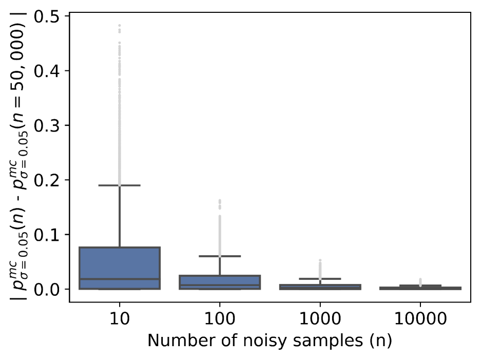
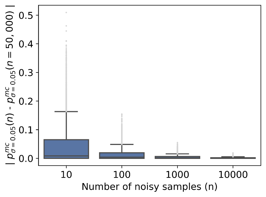
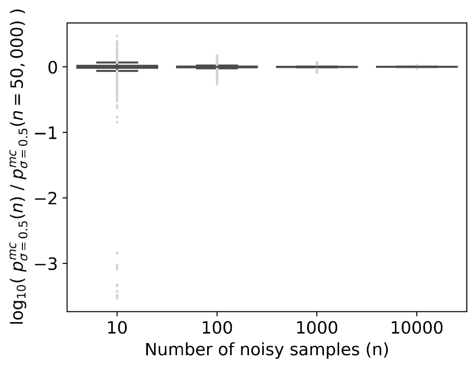
pσmcsubscriptsuperscript𝑝mc𝜎p^{\mathrm{mc}}_{\sigma} replaces the expectation with the sample average of the M𝑀M noisy samples of 𝐱𝐱\mathbf{x} and has been used in prior work (1). While the estimator errors for the Monte-Carlo estimator are technically independent of dimensionality and is given by 𝒪(1/M)𝒪1𝑀\mathcal{O}(1/\sqrt{M}) (14), in practice, for neural networks this requires a large number of random samples to converge to the underlying expectation. For example, for MNIST and CIFAR10 CNNs, it takes around M=10,000𝑀10000M=10,000 samples per point for pσmcsubscriptsuperscript𝑝mc𝜎p^{\mathrm{mc}}_{\sigma} to converge, which is computationally intensive. Thus, we set out to address this problem by developing more efficient analytical estimators of local robustness.

3.2 Robustness Estimation via Linearization

Our goal is to derive computationally efficient estimators of average-case robustness. To this end, we propose to first locally linearize non-linear models and then compute the local robustness of the resulting linear models. This is especially challenging for multi-class classifiers, where the relative orientation of class-wise decision boundaries need to be taken into account to compute local robustness.

Specifically, given a linear model for a three-class classification problem with weights w1,w2,w3subscript𝑤1subscript𝑤2subscript𝑤3w_{1},w_{2},w_{3} and biases b1,b2,b3subscript𝑏1subscript𝑏2subscript𝑏3b_{1},b_{2},b_{3}, such that y=argmaxi{wi𝐱+bii[1,2,3]}𝑦subscript𝑖superscriptsubscript𝑤𝑖top𝐱conditionalsubscript𝑏𝑖𝑖123y=\arg\max_{i}\{w_{i}^{\top}\mathbf{x}+b_{i}\mid i\in[1,2,3]\}, the decision boundary function between classes 111 and 222 is given by y12=(w1w2)𝐱+(b1b2)subscript𝑦12superscriptsubscript𝑤1subscript𝑤2top𝐱subscript𝑏1subscript𝑏2y_{12}=(w_{1}-w_{2})^{\top}\mathbf{x}+(b_{1}-b_{2}). This can be verified as follows: for any 𝐱𝐱\mathbf{x} such that y12=0subscript𝑦120y_{12}=0, we have w1𝐱+b1=w2𝐱+b2superscriptsubscript𝑤1top𝐱subscript𝑏1superscriptsubscript𝑤2top𝐱subscript𝑏2w_{1}^{\top}\mathbf{x}+b_{1}=w_{2}^{\top}\mathbf{x}+b_{2}, making it the decision boundary between classes 1 and 2. If the predicted label at 𝐱𝐱\mathbf{x} is y=1𝑦1y=1, the relevant quantities are the two pairwise difference terms (y12,y13subscript𝑦12subscript𝑦13y_{12},y_{13}) which characterize the decision boundaries of probable misclassifications into classes 222 and 333 respectively. We take this into account and provide the expression for the linear case below.

Notation: For clarity, we represent tensors by collapsing along the ‘class’ dimension, i.e., ai|i=1C:=(a1,a2,ai,ac)assignevaluated-atsubscript𝑎𝑖𝑖1𝐶subscript𝑎1subscript𝑎2subscript𝑎𝑖subscript𝑎𝑐a_{i}~{}\big{|}_{i=1}^{C}:=(a_{1},a_{2},...a_{i},...a_{c}), where for an order-t𝑡t tensor aisubscript𝑎𝑖a_{i}, the expansion ai|i=1Cevaluated-atsubscript𝑎𝑖𝑖1𝐶a_{i}~{}\big{|}_{i=1}^{C} is an order-(t+1)𝑡1(t+1) tensor.

Lemma 3.1.

The local robustness of a multi-class linear model f(𝐱)=𝐰𝐱+b𝑓𝐱superscript𝐰top𝐱𝑏f(\mathbf{x})=\mathbf{w}^{\top}\mathbf{x}+b (with 𝐰d×C𝐰superscript𝑑𝐶\mathbf{w}\in\mathbb{R}^{d\times C} and bC𝑏superscript𝐶b\in\mathbb{R}^{C}) at point 𝐱𝐱\mathbf{x} with respect to a target class t𝑡t is given by the following. Define weights 𝐮i=𝐰t𝐰id,itformulae-sequencesubscript𝐮𝑖subscript𝐰𝑡subscript𝐰𝑖superscript𝑑for-all𝑖𝑡\mathbf{u}_{i}=\mathbf{w}_{t}-\mathbf{w}_{i}\in\mathbb{R}^{d},\forall i\neq t, where 𝐰t,𝐰isubscript𝐰𝑡subscript𝐰𝑖\mathbf{w}_{t},\mathbf{w}_{i} are rows of 𝐰𝐰\mathbf{w} and biases ci=𝐮i𝐱+(btbi)subscript𝑐𝑖superscriptsubscript𝐮𝑖top𝐱subscript𝑏𝑡subscript𝑏𝑖c_{i}={\mathbf{u}_{i}}^{\top}\mathbf{x}+(b_{t}-b_{i})\in\mathbb{R}. Then,

pσrobust(𝐱)=Φ𝐔𝐔(ciσ𝐮i2|i=1itC)subscriptsuperscript𝑝robust𝜎𝐱subscriptΦsuperscript𝐔𝐔topevaluated-atsubscript𝑐𝑖𝜎subscriptnormsubscript𝐮𝑖2𝑖1𝑖𝑡𝐶\displaystyle p^{\mathrm{robust}}_{\sigma}(\mathbf{x})=\Phi_{\mathbf{U}\mathbf{U}^{\top}}\left(\frac{c_{i}}{\sigma\|\mathbf{u}_{i}\|_{2}}~{}\bigg{|}_{\begin{subarray}{c}i=1\\ i\neq t\end{subarray}}^{C}\right)
where𝐔=𝐮i𝐮i2|i=1itC(C1)×dwhere𝐔evaluated-atsubscript𝐮𝑖subscriptnormsubscript𝐮𝑖2𝑖1𝑖𝑡𝐶superscript𝐶1𝑑\displaystyle\mathrm{where}~{}~{}\mathbf{U}=\frac{\mathbf{u}_{i}}{\|\mathbf{u}_{i}\|_{2}}~{}\bigg{|}_{\begin{subarray}{c}i=1\\ i\neq t\end{subarray}}^{C}\in\mathbb{R}^{(C-1)\times d}

and Φ𝐔𝐔subscriptΦsuperscript𝐔𝐔top\Phi_{\mathbf{U}\mathbf{U}^{\top}} is the (C1𝐶1C-1)-dimensional Normal CDF with zero mean and covariance 𝐔𝐔superscript𝐔𝐔top\mathbf{U}\mathbf{U}^{\top}.

Proof Idea.

The proof involves constructing decision boundary functions gi(𝐱)=ft(𝐱)fi(𝐱)subscript𝑔𝑖𝐱subscript𝑓𝑡𝐱subscript𝑓𝑖𝐱g_{i}(\mathbf{x})=f_{t}(\mathbf{x})-f_{i}(\mathbf{x}) and computing the probability pσrobust(𝐱)=Pϵ(i=1itCgi(𝐱+ϵ)>0)subscriptsuperscript𝑝robust𝜎𝐱subscript𝑃italic-ϵsuperscriptsubscript𝑖1𝑖𝑡𝐶subscript𝑔𝑖𝐱italic-ϵ0p^{\text{robust}}_{\sigma}(\mathbf{x})=P_{\epsilon}(\bigcup_{\begin{subarray}{c}i=1\\ i\neq t\end{subarray}}^{C}g_{i}(\mathbf{x}+\epsilon)>0). For Gaussian ϵitalic-ϵ\epsilon, we observe that 𝐮σ𝐮2ϵ𝒩(0,1)similar-tosuperscript𝐮𝜎subscriptnorm𝐮2topitalic-ϵ𝒩01\frac{\mathbf{u}}{\sigma\|\mathbf{u}\|_{2}}^{\top}\epsilon\sim\mathcal{N}(0,1) is also a Gaussian, which applied vectorially results in our usage of ΦΦ\Phi. As convention, we represent 𝐔𝐔\mathbf{U} in a normalized form to ensure that its rows are unit norm. ∎

The proof is in Appendix A.1. The matrix 𝐔𝐔\mathbf{U} exactly captures the geometry of the linear decision boundaries and the covariance matrix 𝐔𝐔superscript𝐔𝐔top\mathbf{U}\mathbf{U}^{\top} encodes the relative similarity between pairs of decision boundaries of different classes.

Remark. For the binary classification case, we get 𝐔𝐔=1superscript𝐔𝐔top1\mathbf{U}\mathbf{U}^{\top}=1 (a scalar), and pσrobust(𝐱)=ϕ(cσ𝐮2)subscriptsuperscript𝑝robust𝜎𝐱italic-ϕ𝑐𝜎subscriptnorm𝐮2p^{\text{robust}}_{\sigma}(\mathbf{x})=\phi(\frac{c}{\sigma\|\mathbf{u}\|_{2}}), where ϕitalic-ϕ\phi is the cdf of the scalar standard normal, which was previously also shown by (13, 15). Hence Lemma 3.1 is a multi-class generalization of (13, 15).

If the decision boundary vectors 𝐮isubscript𝐮𝑖\mathbf{u}_{i} are all orthogonal to each other, then the covariance matrix 𝐔𝐔superscript𝐔𝐔top\mathbf{U}\mathbf{U}^{\top} is identity. However, in practice, we find that the covariance matrix is strongly non-diagonal, indicating that the decision boundaries are not orthogonal to each other. For diagonal covariance matrices, the multivariate Normal CDF (mvn-cdf) can be written as the product of univariate Normal CDFs, which is easy to compute. However, the strong non-diagonal nature of covariance matrices in practice leads to the resulting mvn-cdf not having a closed form solution, and thus needing to be approximated via sampling (16, 17). However, this sampling is performed in the (C1)𝐶1(C-1)-dimensional space as opposed to the d𝑑d-dimensional space that pσmcsubscriptsuperscript𝑝mc𝜎p^{\mathrm{mc}}_{\sigma} samples from. In practice, for classification problems, we often have C<<dmuch-less-than𝐶𝑑C<<d, making sampling in (C1)𝐶1(C-1)-dimensions more efficient. We now discuss the applicability of this solution to non-Gaussian noise.

Lemma 3.2.

(Application to non-Gaussian noise) For high-dimensional data (d𝑑d\rightarrow\infty), Lemma 3.1 generalizes to any coordinate-wise independent noise distribution that satisfies Lyapunov’s condition.

Proof Idea.

Applying Lyupanov’s central limit theorem (18), given ϵsimilar-toitalic-ϵ\epsilon\sim\mathcal{R} is sampled from some distribution \mathcal{R}, we have 𝐮σ𝐮2ϵ=j=1d𝐮jσ𝐮2ϵjd𝒩(0,1)superscript𝐮𝜎subscriptnorm𝐮2topitalic-ϵsuperscriptsubscript𝑗1𝑑subscript𝐮𝑗𝜎subscriptnorm𝐮2subscriptitalic-ϵ𝑗𝑑𝒩01\frac{\mathbf{u}}{\sigma\|\mathbf{u}\|_{2}}^{\top}\epsilon=\sum_{j=1}^{d}\frac{\mathbf{u}_{j}}{\sigma\|\mathbf{u}\|_{2}}\epsilon_{j}~{}~{}\begin{subarray}{c}d\\ \longrightarrow\end{subarray}~{}~{}\mathcal{N}(0,1), which holds as long as the sequence {𝐮j𝐮2ϵj}subscript𝐮𝑗subscriptnorm𝐮2subscriptitalic-ϵ𝑗\{\frac{\mathbf{u}_{j}}{\|\mathbf{u}\|_{2}}\epsilon_{j}\} are independent random variables and satisfy the Lyapunov condition, which encodes the fact that higher-order moments of such distributions progressively shrink. ∎

Thus, as long as the input noise distribution is “well-behaved”, the central limit theorem ensures that the distribution of high-dimensional dot products is Gaussian, thus motivating our use of the mvn-cdf more generally beyond Gaussian input perturbations. We note that it is also possible to easily generalize Lemma 3.1 to non-isotropic Gaussian perturbations with a covariance matrix 𝒞𝒞\mathcal{C}, which only changes the form of the covariance matrix of the mvn-cdf from 𝐔𝐔𝐔𝒞𝐔superscript𝐔𝐔top𝐔𝒞superscript𝐔top\mathbf{U}\mathbf{U}^{\top}\rightarrow\mathbf{U}\mathcal{C}\mathbf{U}^{\top}, which we elaborate in Appendix A.1. In the rest of this paper, we focus on the isotropic case.

3.2.1 Estimator 1: The Taylor Estimator

Using the estimator derived for multi-class linear models in Lemma 3.1, we now derive the Taylor estimator, a local robustness estimator for non-linear models.

Proposition 3.1.

The Taylor estimator for the local robustness of a classifier f𝑓f at point 𝐱𝐱\mathbf{x} with respect to target class t𝑡t is given by linearizing f𝑓f around 𝐱𝐱\mathbf{x} using a first-order Taylor expansion, with decision boundaries gi(𝐱)=ft(𝐱)fi(𝐱)subscript𝑔𝑖𝐱subscript𝑓𝑡𝐱subscript𝑓𝑖𝐱g_{i}(\mathbf{x})=f_{t}(\mathbf{x})-f_{i}(\mathbf{x}), itfor-all𝑖𝑡\forall i\neq t, leading to

pσtaylor(𝐱)=Φ𝐔𝐔(gi(𝐱)σ𝐱gi(𝐱)2|i=1itC)subscriptsuperscript𝑝taylor𝜎𝐱subscriptΦsuperscript𝐔𝐔topevaluated-atsubscript𝑔𝑖𝐱𝜎subscriptnormsubscript𝐱subscript𝑔𝑖𝐱2𝑖1𝑖𝑡𝐶\displaystyle p^{\mathrm{taylor}}_{\sigma}(\mathbf{x})=\Phi_{\mathbf{U}\mathbf{U}^{\top}}\left(\frac{g_{i}(\mathbf{x})}{\sigma\|\nabla_{\mathbf{x}}g_{i}(\mathbf{x})\|_{2}}~{}\bigg{|}_{\begin{subarray}{c}i=1\\ i\neq t\end{subarray}}^{C}\right)

with 𝐔𝐔\mathbf{U} and ΦΦ\Phi defined as in the linear case.

The proof is in Appendix A.1. It involves locally linearizing non-linear decision boundary functions gi(𝐱)subscript𝑔𝑖𝐱g_{i}(\mathbf{x}) using a Taylor series expansion. We expect this estimator to have a small error when the underlying model is well-approximated by a locally linear function in the local neighborhood. We formalize this intuition by computing the estimation error for a quadratic classifier.

Proposition 3.2.

The estimation error of the Taylor estimator for a classifier with a quadratic decision boundary gi(𝐱)=𝐱Ai𝐱+𝐮i𝐱+cisubscript𝑔𝑖𝐱superscript𝐱topsubscript𝐴𝑖𝐱superscriptsubscript𝐮𝑖top𝐱subscript𝑐𝑖g_{i}(\mathbf{x})=\mathbf{x}^{\top}A_{i}\mathbf{x}+\mathbf{u}_{i}^{\top}\mathbf{x}+c_{i} and positive-semidefinite Aisubscript𝐴𝑖A_{i} is upper bounded by

|pσrobust(𝐱)pσtaylor(𝐱)|kσC1i=1itCλmaxAi𝐮i2subscriptsuperscript𝑝robust𝜎𝐱subscriptsuperscript𝑝taylor𝜎𝐱𝑘superscript𝜎𝐶1superscriptsubscriptproduct𝑖1𝑖𝑡𝐶superscriptsubscript𝜆subscript𝐴𝑖subscriptnormsubscript𝐮𝑖2\displaystyle|p^{\mathrm{robust}}_{\sigma}(\mathbf{x})-p^{\mathrm{taylor}}_{\sigma}(\mathbf{x})|\leq k\sigma^{C-1}\prod_{\begin{subarray}{c}i=1\\ i\neq t\end{subarray}}^{C}\frac{\lambda_{\max}^{A_{i}}}{\|\mathbf{u}_{i}\|_{2}}

for noise ϵ𝒩(0,σ2/d)similar-toitalic-ϵ𝒩0superscript𝜎2𝑑\epsilon\sim\mathcal{N}(0,\sigma^{2}/d), in the limit of d𝑑d\rightarrow\infty. Here, λmaxAisuperscriptsubscript𝜆subscript𝐴𝑖\lambda_{\max}^{A_{i}} is the max eigenvalue of Aisubscript𝐴𝑖A_{i}, and k𝑘k is a small problem dependent constant.

The proof is in Appendix A.1. This statement formalizes two key intuitions with regards to the Taylor estimator: (1) the estimation error depends on the size of the local neighborhood σ𝜎\sigma (the smaller the local neighborhood, the more locally linear the model, and the smaller the estimator error), and (2) the estimation error depends on the extent of non-linearity of the underlying function, which is given by the ratio of the max eigenvalue of A𝐴A to the Frobenius norm of the linear term. This measure of non-linearity of a function, called normalized curvature, has also been independently proposed by previous work (19). Notably, if the max eigenvalue is zero, then the function gi(𝐱)subscript𝑔𝑖𝐱g_{i}(\mathbf{x}) is exactly linear, and the estimation error is zero.

3.2.2 Estimator 2: The MMSE Estimator

While the Taylor estimator is more efficient than the naïve one, it has a drawback: its linearization is only faithful at points near the data point and not necessarily at the noisy points. To partly fix this issue, we use a linearization that is faithful to the model over the entire noise distribution, not just near the data point. Linearization has been studied in feature attribution research, which concerns itself with approximating non-linear models with linear ones to produce model explanations (20). In particular, the SmoothGrad (21) technique has been described as the MMSE (minimum mean-squared error) optimal linearization of the model (20, 22) in a Gaussian neighborhood around the data point. Using a similar technique, we propose the MMSE estimator pσmmsesubscriptsuperscript𝑝mmse𝜎p^{\mathrm{mmse}}_{\sigma} as follows.

Proposition 3.3.

The MMSE estimator for the local robustness of a classifier f𝑓f at point 𝐱𝐱\mathbf{x} with respect to target class t𝑡t is given by an MMSE linearization f𝑓f around 𝐱𝐱\mathbf{x}, for decision boundaries gi(𝐱)=ft(𝐱)fi(𝐱)subscript𝑔𝑖𝐱subscript𝑓𝑡𝐱subscript𝑓𝑖𝐱g_{i}(\mathbf{x})=f_{t}(\mathbf{x})-f_{i}(\mathbf{x}), itfor-all𝑖𝑡\forall i\neq t, leading to

pσmmse(𝐱)=Φ𝐔𝐔(g~i(𝐱)σ𝐱g~i(𝐱)2|i=1itC)subscriptsuperscript𝑝mmse𝜎𝐱subscriptΦsuperscript𝐔𝐔topevaluated-atsubscript~𝑔𝑖𝐱𝜎subscriptnormsubscript𝐱subscript~𝑔𝑖𝐱2𝑖1𝑖𝑡𝐶\displaystyle p^{\mathrm{mmse}}_{\sigma}(\mathbf{x})=\Phi_{\mathbf{U}\mathbf{U}^{\top}}\left(\frac{\tilde{g}_{i}(\mathbf{x})}{\sigma\|\nabla_{\mathbf{x}}\tilde{g}_{i}(\mathbf{x})\|_{2}}~{}\bigg{|}_{\begin{subarray}{c}i=1\\ i\neq t\end{subarray}}^{C}\right)
whereg~i(𝐱)=1Nj=1Ngi(𝐱+ϵ),ϵ𝒩(0,σ2)formulae-sequencewheresubscript~𝑔𝑖𝐱1𝑁superscriptsubscript𝑗1𝑁subscript𝑔𝑖𝐱italic-ϵsimilar-toitalic-ϵ𝒩0superscript𝜎2\displaystyle\mathrm{where}~{}~{}\tilde{g}_{i}(\mathbf{x})=\frac{1}{N}\sum_{j=1}^{N}g_{i}(\mathbf{x}+\epsilon)~{},~{}\epsilon\sim\mathcal{N}(0,\sigma^{2})

with 𝐔𝐔\mathbf{U} and ΦΦ\Phi defined as in the linear case, and N𝑁N is the number of perturbations.

The proof is in Appendix A.1. It involves creating a randomized smooth model (5) from the base model and computing the decision boundaries of this smooth model. We show, for the first time, that performing such randomization helps compute robustness information for the original base model. We now compute the estimation error of the MMSE estimator.

Proposition 3.4.

The estimation error of the MMSE estimator for a classifier with a quadratic decision boundary gi(𝐱)=𝐱Ai𝐱+𝐮i𝐱+cisubscript𝑔𝑖𝐱superscript𝐱topsubscript𝐴𝑖𝐱superscriptsubscript𝐮𝑖top𝐱subscript𝑐𝑖g_{i}(\mathbf{x})=\mathbf{x}^{\top}A_{i}\mathbf{x}+\mathbf{u}_{i}^{\top}\mathbf{x}+c_{i} and positive-semidefinite Aisubscript𝐴𝑖A_{i} is upper bounded by

|pσrobust(𝐱)pσmmse(𝐱)|kσC1i=1itCλmaxAiλmeanAi𝐮i2subscriptsuperscript𝑝robust𝜎𝐱subscriptsuperscript𝑝mmse𝜎𝐱𝑘superscript𝜎𝐶1superscriptsubscriptproduct𝑖1𝑖𝑡𝐶superscriptsubscript𝜆subscript𝐴𝑖superscriptsubscript𝜆meansubscript𝐴𝑖subscriptnormsubscript𝐮𝑖2\displaystyle|p^{\mathrm{robust}}_{\sigma}(\mathbf{x})-p^{\mathrm{mmse}}_{\sigma}(\mathbf{x})|\leq k\sigma^{C-1}\prod_{\begin{subarray}{c}i=1\\ i\neq t\end{subarray}}^{C}\frac{\lambda_{\max}^{A_{i}}-\lambda_{\text{mean}}^{A_{i}}}{\|\mathbf{u}_{i}\|_{2}}

for noise ϵ𝒩(0,σ2/d)similar-toitalic-ϵ𝒩0superscript𝜎2𝑑\epsilon\sim\mathcal{N}(0,\sigma^{2}/d), in the limit of d𝑑d\rightarrow\infty and N𝑁N\rightarrow\infty. Here, λmaxAi,λmeanAisuperscriptsubscript𝜆subscript𝐴𝑖superscriptsubscript𝜆meansubscript𝐴𝑖\lambda_{\max}^{A_{i}},\lambda_{\text{mean}}^{A_{i}} are the maximum and mean eigenvalue of Aisubscript𝐴𝑖A_{i} respectively, and k𝑘k is a small problem dependent constant.

The proof is in Appendix A.1. The result above highlights two aspects of the MMSE estimator: (1) it incurs a smaller estimation error than the Taylor estimator, and (2) even in the limit of large number of samples N𝑁N\rightarrow\infty, the error of the MMSE estimator is non-zero, except when λmeanAi=λmaxAisuperscriptsubscript𝜆meansubscript𝐴𝑖superscriptsubscript𝜆subscript𝐴𝑖\lambda_{\text{mean}}^{A_{i}}=\lambda_{\max}^{A_{i}}. For PSD matrices, this implies that Aisubscript𝐴𝑖A_{i} is a multiple of the identity. 222When d𝑑d\rightarrow\infty, ϵAϵ=λϵ2=λσ2superscriptitalic-ϵtop𝐴italic-ϵ𝜆superscriptnormitalic-ϵ2𝜆superscript𝜎2\epsilon^{\top}A\epsilon=\lambda\|\epsilon\|^{2}=\lambda\sigma^{2} is a constant, and thus an isotropic quadratic function resembles a linear one in this neighborhood.

3.2.3 Approximating ΦΦ\Phi

One drawback of the Taylor and MMSE estimators is their use of the mvn-cdf, which does not have a closed form solution and can cause the estimators to be slow for settings with a large number of classes C𝐶C. In addition, the mvn-cdf makes these estimators non-differentiable, which is inconvenient for applications which require differentiating pσrobustsubscriptsuperscript𝑝robust𝜎p^{\mathrm{robust}}_{\sigma}. To alleviate these issues, we wish to approximate the mvn-cdf with an analytical closed-form expression. As CDFs are monotonically increasing functions, the approximation should also be monotonically increasing.

To this end, it has been previously shown that the univariate Normal CDF ϕitalic-ϕ\phi is well-approximated by the sigmoid function (23). It is also known that when 𝐔𝐔=Isuperscript𝐔𝐔top𝐼\mathbf{U}\mathbf{U}^{\top}=I, mvn-cdf is given by Φ(𝐱)=iϕ(𝐱i)Φ𝐱subscriptproduct𝑖italic-ϕsubscript𝐱𝑖\Phi(\mathbf{x})=\prod_{i}\phi(\mathbf{x}_{i}), i.e., it is given by the product of the univariate normal CDFs. Thus, we may choose to approximate Φ(𝐱)=isigmoid(𝐱)Φ𝐱subscriptproduct𝑖sigmoid𝐱\Phi(\mathbf{x})=\prod_{i}\text{sigmoid}(\mathbf{x}). However, when the inputs are small, this can be simplified as follows:

ΦI(𝐱)=iϕ(𝐱i)i11+exp(𝐱i)(see (23))subscriptΦ𝐼𝐱subscriptproduct𝑖italic-ϕsubscript𝐱𝑖subscriptproduct𝑖11subscript𝐱𝑖see (23)\displaystyle\Phi_{I}(\mathbf{x})=\prod_{i}\phi(\mathbf{x}_{i})\approx\prod_{i}\frac{1}{1+\exp(-\mathbf{x}_{i})}~{}~{}~{}(\text{see ~{}\cite[cite]{(\@@bibref{Number}{hendrycks2016gaussian}{}{})}})
=11+iexp(𝐱i)+j,kexp(𝐱j𝐱k)+absent11subscript𝑖subscript𝐱𝑖subscript𝑗𝑘subscript𝐱𝑗subscript𝐱𝑘\displaystyle=\frac{1}{1+\sum_{i}\exp(-\mathbf{x}_{i})+\sum_{j,k}\exp(-\mathbf{x}_{j}-\mathbf{x}_{k})+...}
11+iexp(𝐱i)(for𝐱ii)absent11subscript𝑖subscript𝐱𝑖forsubscript𝐱𝑖for-all𝑖\displaystyle\approx\frac{1}{1+\sum_{i}\exp(-\mathbf{x}_{i})}~{}~{}~{}(\text{for}~{}~{}\mathbf{x}_{i}\rightarrow\infty~{}~{}\forall i)

We call the final expression the “multivariate sigmoid” (mv-sigmoid) which serves as our approximation of mvn-cdf, especially at the tails of the distribution. While we expect estimators using mv-sigmoid to approximate ones using mvn-cdf only when 𝐔𝐔=𝐈superscript𝐔𝐔top𝐈\mathbf{U}\mathbf{U}^{\top}=\mathbf{I}, we find experimentally that the approximation works well even for practical values of the covariance matrix 𝐔𝐔superscript𝐔𝐔top\mathbf{U}\mathbf{U}^{\top}. Using this approximation to substitute mv-sigmoid for mvn-cdf in the pσtaylorsubscriptsuperscript𝑝taylor𝜎p^{\mathrm{taylor}}_{\sigma} and pσmmsesubscriptsuperscript𝑝mmse𝜎p^{\mathrm{mmse}}_{\sigma} estimators yields the pσtaylor_mvssubscriptsuperscript𝑝taylor_mvs𝜎p^{\mathrm{taylor\_mvs}}_{\sigma} and pσmmse_mvssubscriptsuperscript𝑝mmse_mvs𝜎p^{\mathrm{mmse\_mvs}}_{\sigma} estimators, respectively.

Relationship with Softmax.

A common method to estimate the confidence of model predictions is to use the softmax function applied to the logits fi(𝐱)subscript𝑓𝑖𝐱f_{i}(\mathbf{x}) of a model. We note that softmax is identical to mv-sigmoid when directly applied to the logits of neural networks:

softmaxt(fi(𝐱)|i=1C)=exp(ft(𝐱))i=1Cexp(fi(𝐱))=subscriptsoftmax𝑡evaluated-atsubscript𝑓𝑖𝐱𝑖1𝐶subscript𝑓𝑡𝐱superscriptsubscript𝑖1𝐶subscript𝑓𝑖𝐱absent\displaystyle\text{softmax}_{t}\left(f_{i}(\mathbf{x})~{}\Big{|}_{\begin{subarray}{c}i=1\end{subarray}}^{C}\right)=\frac{\exp(f_{t}(\mathbf{x}))}{\sum_{i=1}^{C}\exp(f_{i}(\mathbf{x}))}=
11+i=1itCexp(fi(𝐱)ft(𝐱))=mv-sigmoid(gi(𝐱)|i=1itC)11superscriptsubscript𝑖1𝑖𝑡𝐶subscript𝑓𝑖𝐱subscript𝑓𝑡𝐱mv-sigmoidevaluated-atsubscript𝑔𝑖𝐱𝑖1𝑖𝑡𝐶\displaystyle\frac{1}{1+\sum\limits_{\begin{subarray}{c}i=1\\ i\neq t\end{subarray}}^{C}\exp(f_{i}(\mathbf{x})-f_{t}(\mathbf{x}))}=\text{mv-sigmoid}\left(g_{i}(\mathbf{x})~{}\Big{|}_{\begin{subarray}{c}i=1\\ i\neq t\end{subarray}}^{C}\right)

Recall that gi(𝐱)=ft(𝐱)fi(𝐱)subscript𝑔𝑖𝐱subscript𝑓𝑡𝐱subscript𝑓𝑖𝐱g_{i}(\mathbf{x})=f_{t}(\mathbf{x})-f_{i}(\mathbf{x}) is the decision boundary function. Note that this equivalence only holds for the specific case of logits. Comparing the expressions of softmax applied to logits above and the Taylor estimator, we notice that they are only different in that the Taylor estimator divides by the gradient norm, and uses the mvn-cdf function instead of mv-sigmoid. Given this similarity to the Taylor estimator, it is reasonable to ask whether softmax applied to logits (henceforth pTsoftmaxsubscriptsuperscript𝑝softmax𝑇p^{\text{softmax}}_{T} for softmax with temperature T𝑇T) itself can be a “good enough” estimator of pσrobustsubscriptsuperscript𝑝robust𝜎p^{\text{robust}}_{\sigma} in practice. In other words, does pTsoftmaxsubscriptsuperscript𝑝softmax𝑇p^{\text{softmax}}_{T} well-approximate pσrobustsubscriptsuperscript𝑝robust𝜎p^{\text{robust}}_{\sigma} in certain settings?

In general, this cannot hold because softmax does not take in information about 𝐔𝐔superscript𝐔𝐔top\mathbf{U}\mathbf{U}^{\top}, nor does it use the gradient information used in all of our estimators, although the temperature parameter T𝑇T can serve as a substitute for σ𝜎\sigma in our expressions. In Appendix A.1, we provide a theoretical result for a restricted linear setting where softmax can indeed match the behavior of pσtaylor_mvssubscriptsuperscript𝑝taylor_mvs𝜎p^{\mathrm{taylor\_mvs}}_{\sigma}, which happens precisely when 𝐔𝐔=𝐈superscript𝐔𝐔top𝐈\mathbf{U}\mathbf{U}^{\top}=\mathbf{I} and all the class-wise gradients are equal. In the next section, we demonstrate empirically that the softmax estimator pTsoftmaxsubscriptsuperscript𝑝softmax𝑇p^{\text{softmax}}_{T} is a poor estimator of average robustness in practice.

4 Empirical Evaluation

In this section, we first evaluate the estimation errors and computational efficiency of the analytical estimators, and then evaluate the impact of robustness training within models on these estimation errors. Then, we analyze the relationship between average-case robustness and softmax probability. Lastly, we demonstrate the usefulness of local robustness and its analytical estimators in real-world applications. Key results are discussed in this section and full results are in Appendix A.4.

Datasets and models. We evaluate the estimators on four datasets: MNIST (24), FashionMNIST (25), CIFAR10 (26), and CIFAR100 (26). For MNIST and FashionMNIST, we train linear models and CNNs to perform classification. For CIFAR10 and CIFAR100, we train ResNet18 (27) models to perform classification. We train the ResNet18 models using varying levels of gradient norm regularization (λ𝜆\lambda) to obtain models with varying levels of robustness. The experiments below use each dataset’s full test set, each consisting of 10,000 points. Additional details about the datasets and models are described in Appendix A.2 and A.3.

4.1 Evaluation of the estimation errors of analytical estimators

To empirically evaluate the estimation error of our estimators, we calculate pσrobustsubscriptsuperscript𝑝robust𝜎p^{\mathrm{robust}}_{\sigma} for each model using pσmcsubscriptsuperscript𝑝mc𝜎p^{\mathrm{mc}}_{\sigma}, pσtaylorsubscriptsuperscript𝑝taylor𝜎p^{\mathrm{taylor}}_{\sigma}, pσmmsesubscriptsuperscript𝑝mmse𝜎p^{\mathrm{mmse}}_{\sigma}, pσtaylor_mvssubscriptsuperscript𝑝taylor_mvs𝜎p^{\mathrm{taylor\_mvs}}_{\sigma}, pσmmse_mvssubscriptsuperscript𝑝mmse_mvs𝜎p^{\mathrm{mmse\_mvs}}_{\sigma}, and pTsoftmaxsubscriptsuperscript𝑝softmax𝑇p^{\mathrm{softmax}}_{T} for different σ𝜎\sigma values. For pσmcsubscriptsuperscript𝑝mc𝜎p^{\mathrm{mc}}_{\sigma}, pσmmsesubscriptsuperscript𝑝mmse𝜎p^{\mathrm{mmse}}_{\sigma}, and pσmmse_mvssubscriptsuperscript𝑝mmse_mvs𝜎p^{\mathrm{mmse\_mvs}}_{\sigma}, we use a sample size at which these estimators have converged (n=10000,500,and 500𝑛10000500and 500n=10000,500,\text{and }500, respectively). (Convergence analyses are in Appendix A.4.) We take the monte-carlo estimator as the gold standard estimate of pσrobustsubscriptsuperscript𝑝𝑟𝑜𝑏𝑢𝑠𝑡𝜎p^{robust}_{\sigma}), and compute the absolute and relative difference between pσmcsubscriptsuperscript𝑝mc𝜎p^{\mathrm{mc}}_{\sigma} and the other estimators to evaluate their estimation errors.

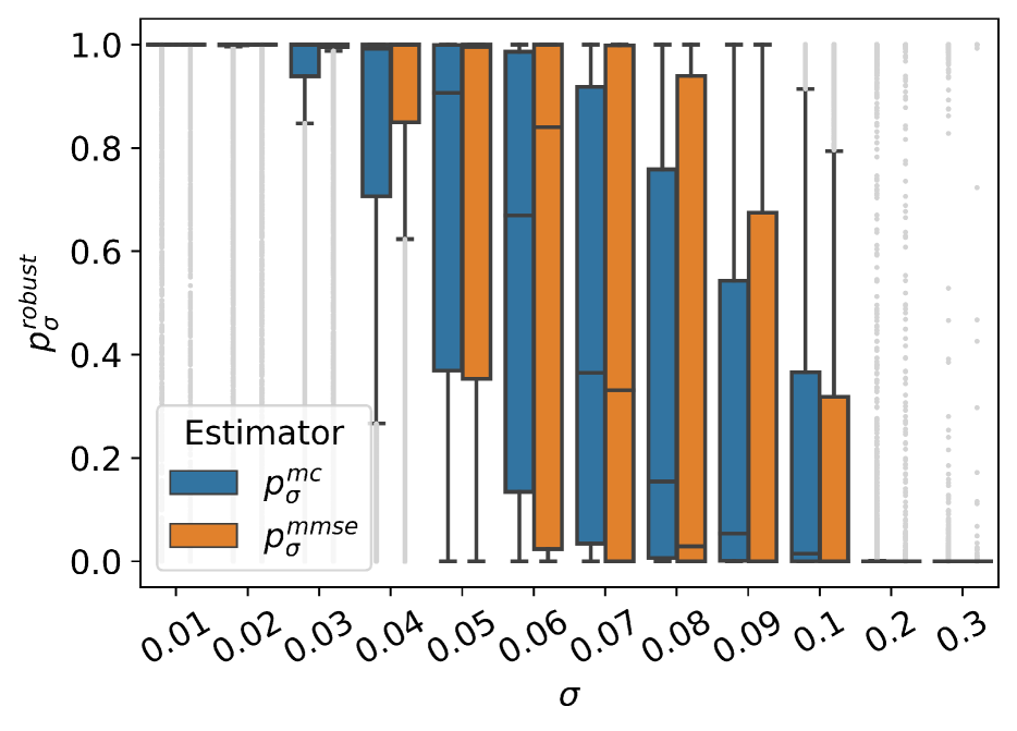
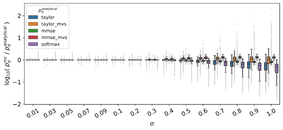
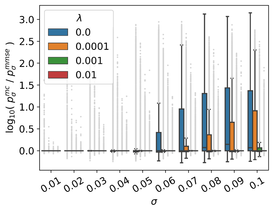
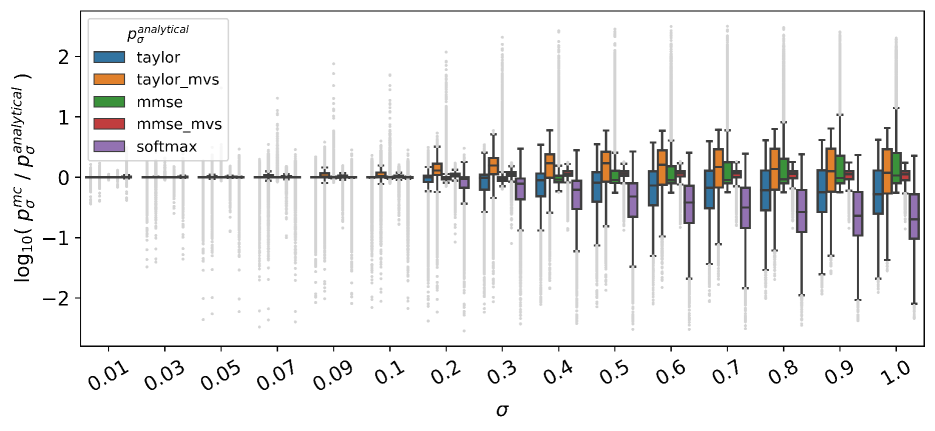
The performance of the estimators for the FashionMNIST CNN model is shown in Figure 1(a). The results indicate that pσmmse_mvssubscriptsuperscript𝑝mmse_mvs𝜎p^{\mathrm{mmse\_mvs}}_{\sigma} and pσmmsesubscriptsuperscript𝑝mmse𝜎p^{\mathrm{mmse}}_{\sigma} are the best estimators of pσrobustsubscriptsuperscript𝑝robust𝜎p^{\mathrm{robust}}_{\sigma}, followed closely by pσtaylor_mvssubscriptsuperscript𝑝taylor_mvs𝜎p^{\mathrm{taylor\_mvs}}_{\sigma} and pσtaylorsubscriptsuperscript𝑝taylor𝜎p^{\mathrm{taylor}}_{\sigma}, trailed by pTsoftmaxsubscriptsuperscript𝑝softmax𝑇p^{\mathrm{softmax}}_{T}. This is consistent with the theory in Section 3, where the analytical estimation errors of pσmmsesubscriptsuperscript𝑝𝑚𝑚𝑠𝑒𝜎p^{mmse}_{\sigma} are lower than pσtaylorsubscriptsuperscript𝑝𝑡𝑎𝑦𝑙𝑜𝑟𝜎p^{taylor}_{\sigma}.

The results also confirm that the smaller the noise neighborhood σ𝜎\sigma, the more accurately the estimators compute pσrobustsubscriptsuperscript𝑝robust𝜎p^{\mathrm{robust}}_{\sigma}. For the MMSE and Taylor estimators, this is because their linear approximation of the model around the input is more faithful for smaller σ𝜎\sigma. As expected, when the model is linear, pσtaylorsubscriptsuperscript𝑝taylor𝜎p^{\mathrm{taylor}}_{\sigma} and pσmmsesubscriptsuperscript𝑝mmse𝜎p^{\mathrm{mmse}}_{\sigma} accurately compute pσrobustsubscriptsuperscript𝑝robust𝜎p^{\mathrm{robust}}_{\sigma} for all σ𝜎\sigma’s (Appendix A.4). For the softmax estimator, pTsoftmaxsubscriptsuperscript𝑝softmax𝑇p^{\mathrm{softmax}}_{T} values are constant over σ𝜎\sigma and this particular model has high pTsoftmaxsubscriptsuperscript𝑝softmax𝑇p^{\mathrm{softmax}}_{T} values for most points. Thus, for small σ𝜎\sigma’s where pσrobustsubscriptsuperscript𝑝robust𝜎p^{\mathrm{robust}}_{\sigma} is near one, pTsoftmaxsubscriptsuperscript𝑝softmax𝑇p^{\mathrm{softmax}}_{T} happens to approximate pσrobustsubscriptsuperscript𝑝robust𝜎p^{\mathrm{robust}}_{\sigma} for this model. Examples of images with varying levels of noise (σ𝜎\sigma) are in Appendix A.4.

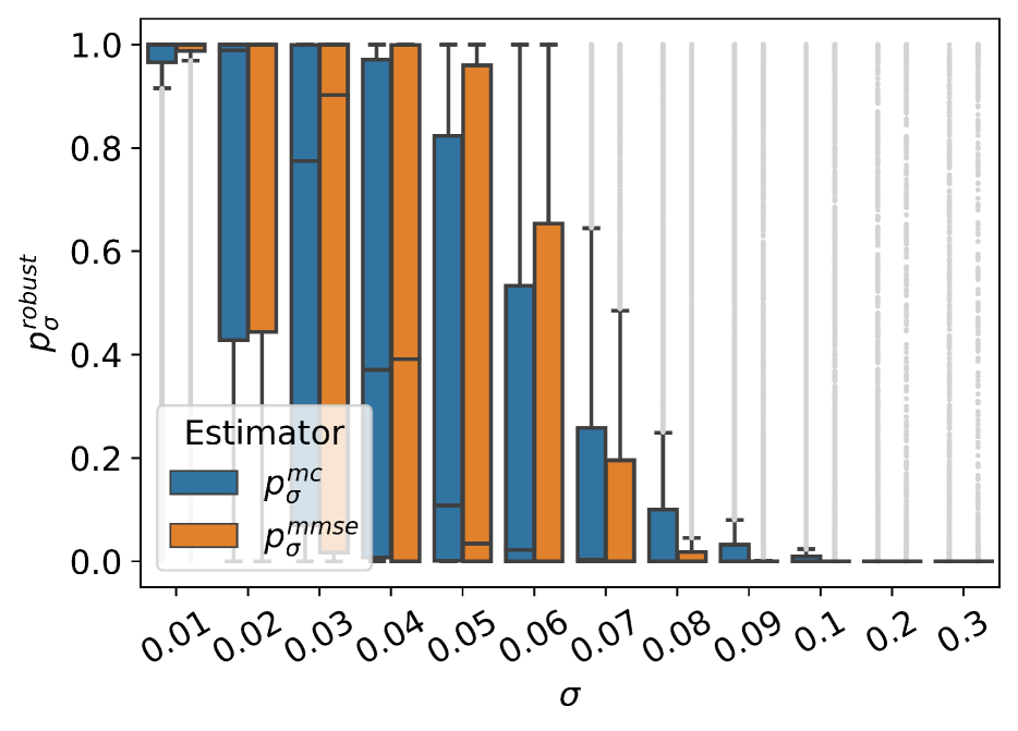
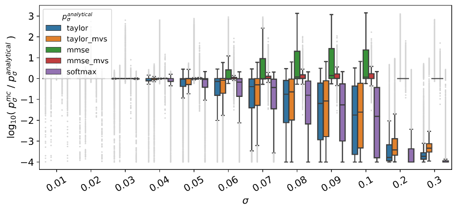
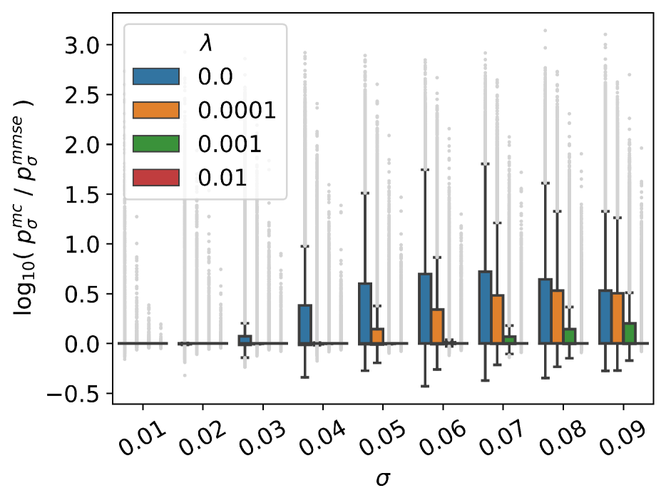
Impact of robust training on estimation errors. The performance of pσmmsesubscriptsuperscript𝑝mmse𝜎p^{\mathrm{mmse}}_{\sigma} for CIFAR10 ResNet18 models of varying levels of robustness is shown in Figure 1(b). The results indicate that for more robust models (larger λ𝜆\lambda), the estimator is more accurate over a larger σ𝜎\sigma. This is because gradient norm regularization leads to models that are more locally linear (19), making the estimator’s linear approximation of the model around the input more accurate over a larger σ𝜎\sigma, making its pσrobustsubscriptsuperscript𝑝robust𝜎p^{\mathrm{robust}}_{\sigma} values more accurate.

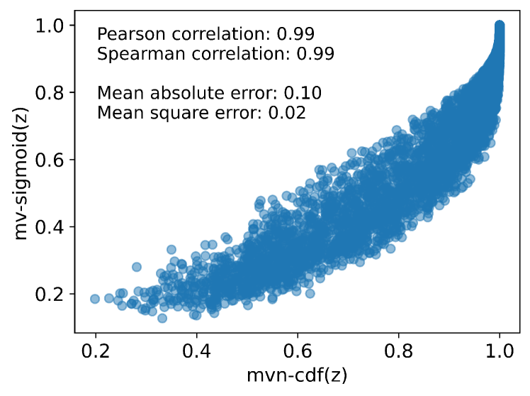
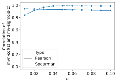
Evaluating estimation error of mv-sigmoid. To examine mv-sigmoid’s approximation of mvn-cdf, we compute both functions using the same inputs (z=gi(𝐱)σ𝐱gi(𝐱)2|i=1itC𝑧evaluated-atsubscript𝑔𝑖𝐱𝜎subscriptnormsubscript𝐱subscript𝑔𝑖𝐱2𝑖1𝑖𝑡𝐶z~{}=~{}\frac{g_{i}(\mathbf{x})}{\sigma\|\nabla_{\mathbf{x}}g_{i}(\mathbf{x})\|_{2}}|_{\begin{subarray}{c}i=1\\ i\neq t\end{subarray}}^{C}, as described in Proposition 3.1) for the CIFAR10 ResNet18 model for different σ𝜎\sigma. The plot of mv-sigmoid(z) against mvn-cdf(z) for σ=0.05𝜎0.05\sigma=0.05 is shown in Figure 2. The results indicate that the two functions are strongly positively correlated with low approximation error, suggesting that mv-sigmoid approximates the mvn-cdf well in practice.
Refer to caption
(a) FashionMNIST, CNN
Comparing estimator errors
Refer to caption
(b) CIFAR10, ResNet18
Varying model robustness
Figure 1: Empirical evaluation of analytical estimators. (a) The smaller the noise neighborhood σ𝜎\sigma, the more accurately the estimators compute pσrobustsubscriptsuperscript𝑝robust𝜎p^{\mathrm{robust}}_{\sigma}. pσmmsesubscriptsuperscript𝑝mmse𝜎p^{\mathrm{mmse}}_{\sigma} and pσmmse_mvssubscriptsuperscript𝑝mmse_mvs𝜎p^{\mathrm{mmse\_mvs}}_{\sigma} are the best estimators of pσrobustsubscriptsuperscript𝑝robust𝜎p^{\mathrm{robust}}_{\sigma}, followed closely by pσtaylor_mvssubscriptsuperscript𝑝taylor_mvs𝜎p^{\mathrm{taylor\_mvs}}_{\sigma} and pσtaylorsubscriptsuperscript𝑝taylor𝜎p^{\mathrm{taylor}}_{\sigma}, trailed by pTsoftmaxsubscriptsuperscript𝑝softmax𝑇p^{\mathrm{softmax}}_{T}. (b) For more robust models, the estimators compute pσrobustsubscriptsuperscript𝑝robust𝜎p^{\mathrm{robust}}_{\sigma} more accurately over a larger σ𝜎\sigma. Together, these results indicate that the analytical estimators accurately compute pσrobustsubscriptsuperscript𝑝robust𝜎p^{\mathrm{robust}}_{\sigma}.
Refer to caption
Figure 2: Correlation of mvn-cdf(z) and mv-sigmoid(z) for the CIFAR10 ResNet18 model. The formulation of z𝑧z is described in Section 4.1. In practice, mv-sigmoid approximates mvn-cdf well.
Estimator # samples (n𝑛n) CPU runtime (h:m:s) GPU Runtime (h:m:s)
pσmcsubscriptsuperscript𝑝mc𝜎p^{\mathrm{mc}}_{\sigma}
n=10000𝑛10000n=10000
1:41:11
0:19:56
pσtaylorsubscriptsuperscript𝑝taylor𝜎p^{\mathrm{taylor}}_{\sigma} N/A 0:00:08 0:00:02
pσmmsesubscriptsuperscript𝑝mmse𝜎p^{\mathrm{mmse}}_{\sigma}
n=5𝑛5n=5
0:00:41
0:00:06
Table 1: Runtimes of pσrobustsubscriptsuperscript𝑝robust𝜎p^{\mathrm{robust}}_{\sigma} estimators. Each estimator computes pσ=0.1robustsubscriptsuperscript𝑝robust𝜎0.1p^{\mathrm{robust}}_{\sigma={0.1}} for the CIFAR10 ResNet18 model for 50 data points. Estimators that use sampling use the minimum number of samples necessary for convergence. Runtimes are in the format of hour:minute:second. The GPU used was a Tesla V100. The analytical estimators (pσtaylorsubscriptsuperscript𝑝taylor𝜎p^{\mathrm{taylor}}_{\sigma} and pσmmsesubscriptsuperscript𝑝mmse𝜎p^{\mathrm{mmse}}_{\sigma}) are more efficient than the naïve estimator (pσmcsubscriptsuperscript𝑝mc𝜎p^{\mathrm{mc}}_{\sigma}).

Refer to caption
(a) CIFAR10
Non-robust model (λ=0𝜆0\lambda=0)
Refer to caption
(b) CIFAR10 and CIFAR100
Varying model robustness
Refer to caption
(c) CIFAR10
Robust model (λ=0.01𝜆0.01\lambda=0.01)
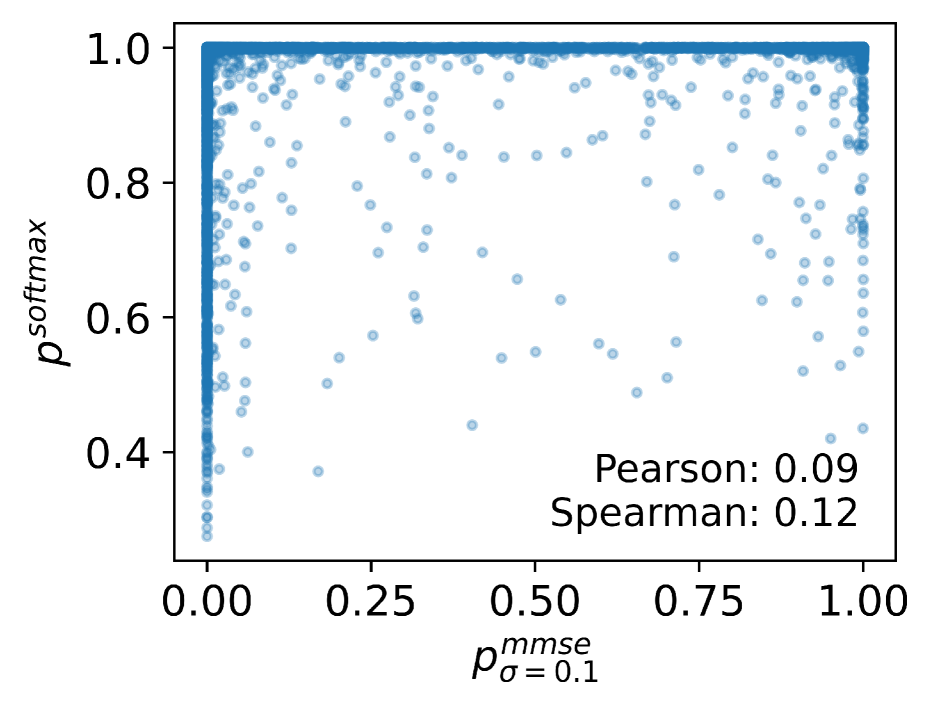
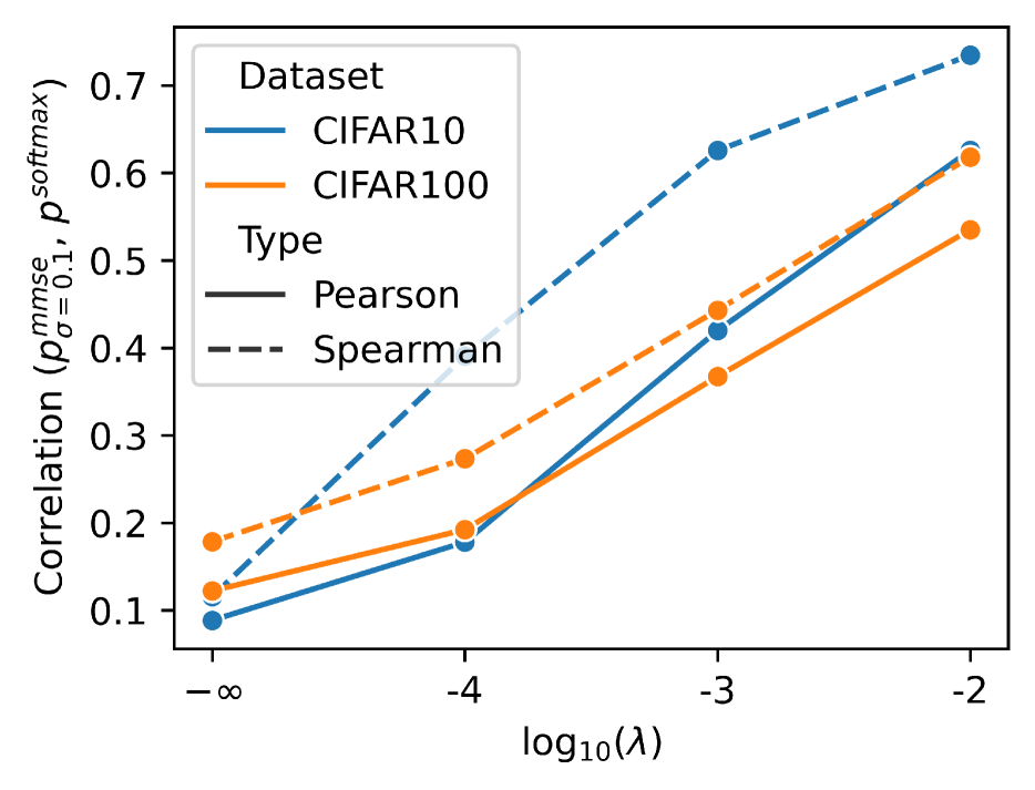
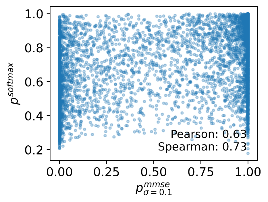
Figure 3: Relationship between pσrobustsubscriptsuperscript𝑝robust𝜎p^{\mathrm{robust}}_{\sigma} and pTsoftmaxsubscriptsuperscript𝑝softmax𝑇p^{\mathrm{softmax}}_{T} for CIFAR10 and CIFAR100 ResNet18 models. (a) For a non-robust model, pσrobustsubscriptsuperscript𝑝robust𝜎p^{\mathrm{robust}}_{\sigma} and pTsoftmaxsubscriptsuperscript𝑝softmax𝑇p^{\mathrm{softmax}}_{T} are not strongly correlated. (b) As model robustness increases, the two quantities become more correlated. (c) However, even for robust models, the relationship between pσrobustsubscriptsuperscript𝑝robust𝜎p^{\mathrm{robust}}_{\sigma} and pTsoftmaxsubscriptsuperscript𝑝softmax𝑇p^{\mathrm{softmax}}_{T} is mild. Together, these results indicate that, consistent with the theory in Section 3, pTsoftmaxsubscriptsuperscript𝑝softmax𝑇p^{\mathrm{softmax}}_{T} is not a good estimator for pσrobustsubscriptsuperscript𝑝robust𝜎p^{\mathrm{robust}}_{\sigma} in general settings.
Refer to caption
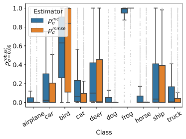
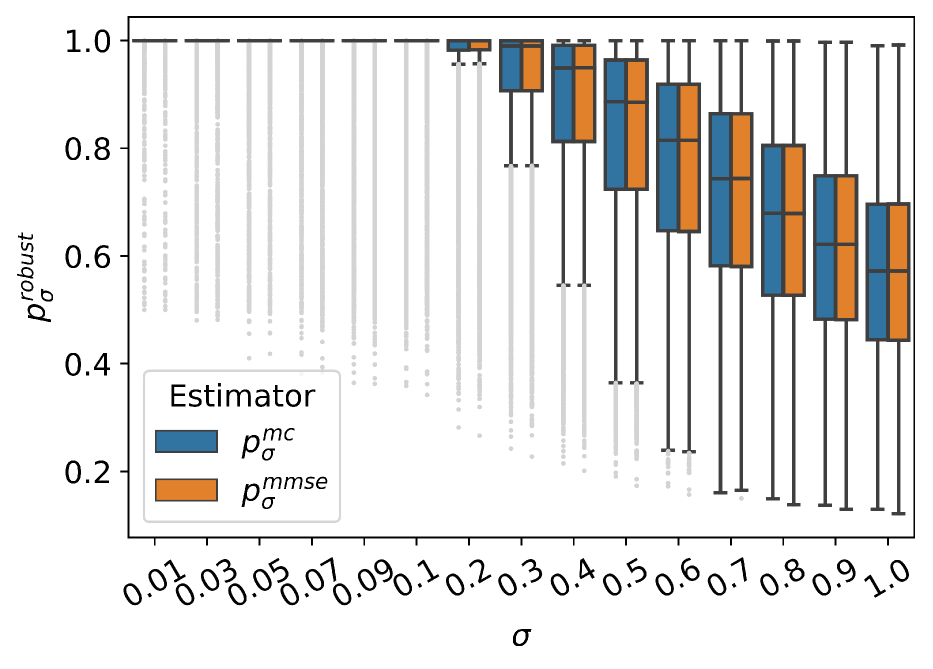
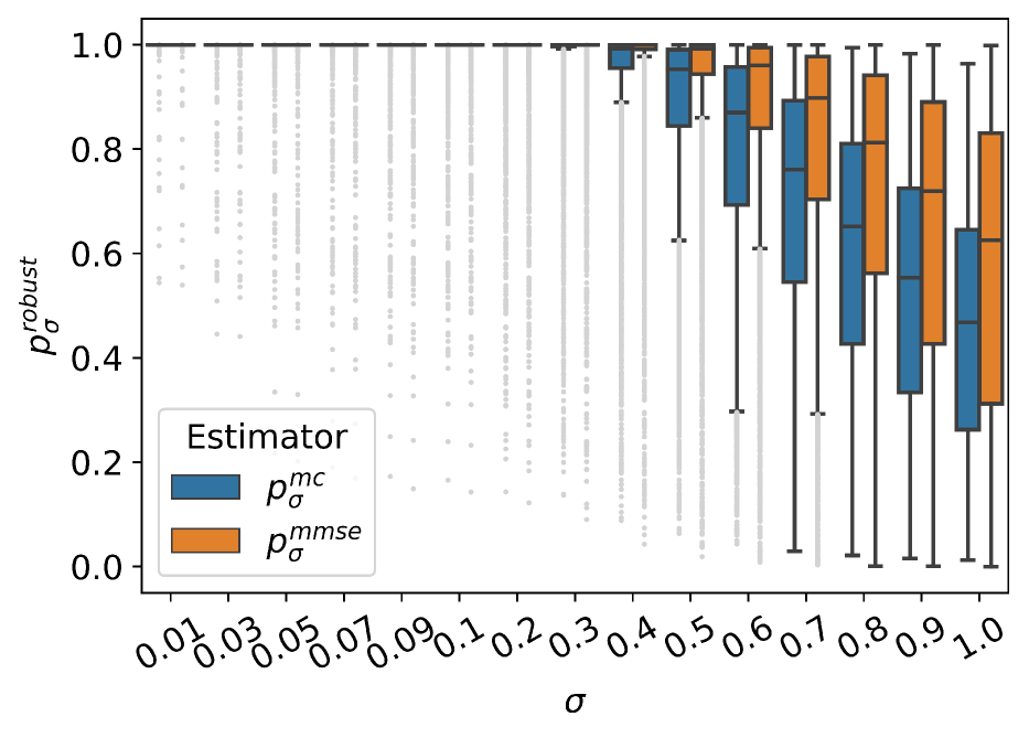
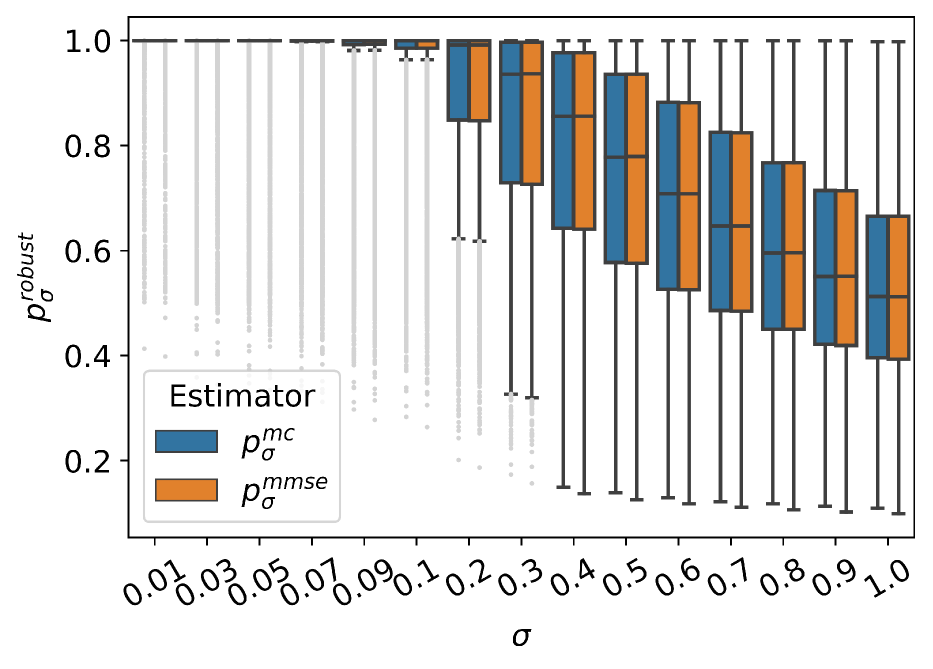
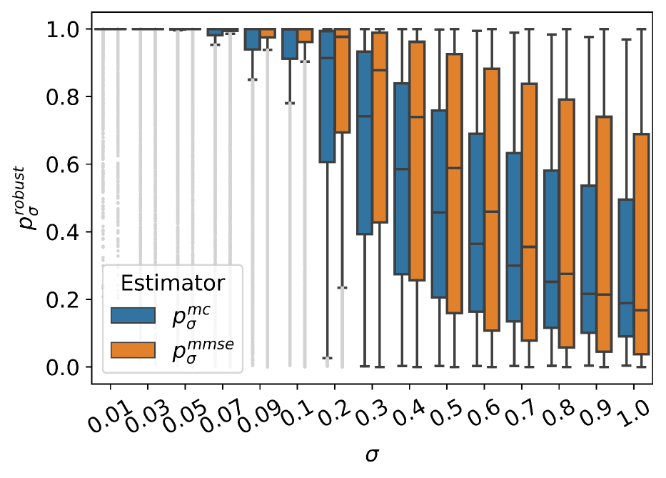
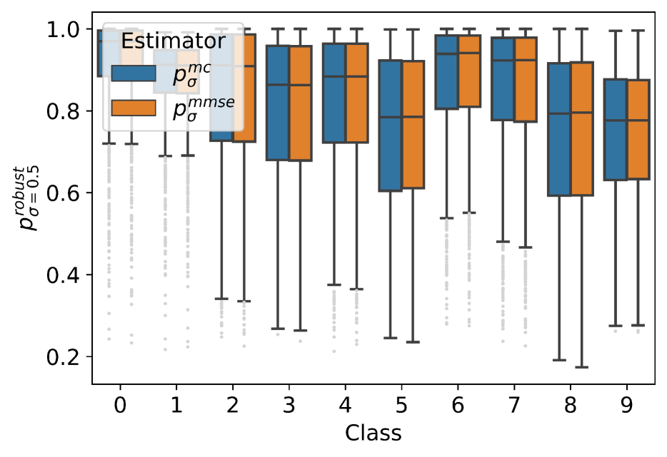
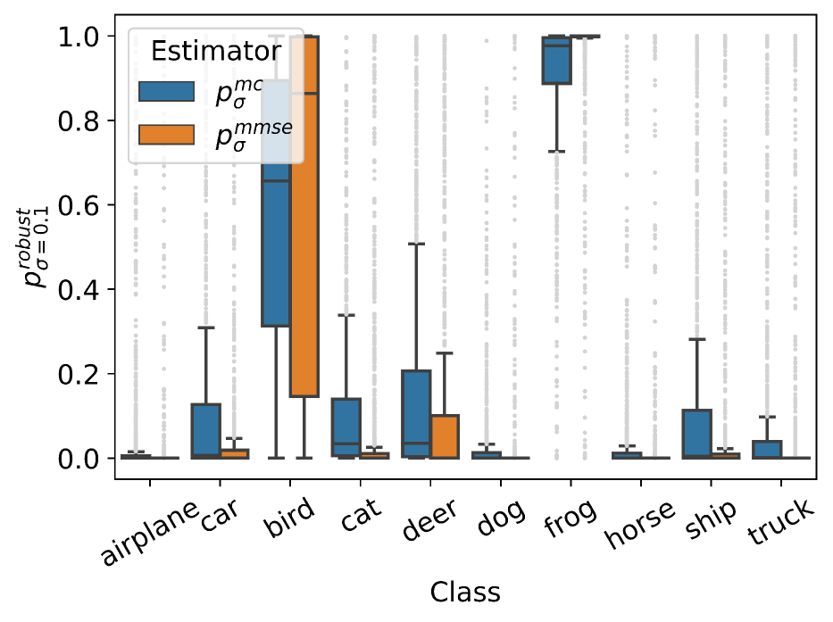
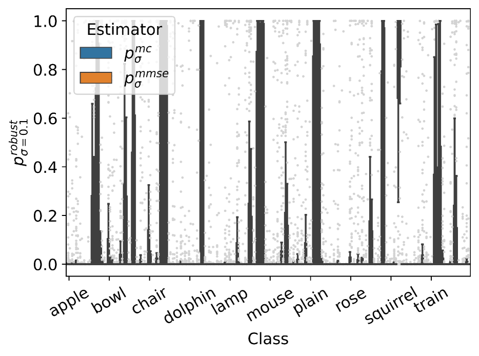
Figure 4: Local robustness bias among classes for the ResNet18 CIFAR10 model. pσrobustsubscriptsuperscript𝑝robust𝜎p^{\mathrm{robust}}_{\sigma} reveals that the model is less locally robust for some classes than for others. The analytical estimator pσmmsesubscriptsuperscript𝑝mmse𝜎p^{\mathrm{mmse}}_{\sigma} properly captures this model bias.

4.2 Evaluation of computational efficiency of analytical estimators

We examine the efficiency of the estimators by measuring their runtimes when calculating pσ=0.1robustsubscriptsuperscript𝑝robust𝜎0.1p^{\mathrm{robust}}_{\sigma={0.1}} for the CIFAR10 ResNet18 model for 50 points. Runtimes are displayed in Table 1. They indicate that pσtaylorsubscriptsuperscript𝑝taylor𝜎p^{\mathrm{taylor}}_{\sigma} and pσmmsesubscriptsuperscript𝑝mmse𝜎p^{\mathrm{mmse}}_{\sigma} perform 35x and 17x faster than pσmcsubscriptsuperscript𝑝mc𝜎p^{\mathrm{mc}}_{\sigma}, respectively. Additional runtimes are in Appendix A.4.

4.3 Softmax probability is not a good proxy for average-case robustness

To examine the relationship between pσrobustsubscriptsuperscript𝑝robust𝜎p^{\mathrm{robust}}_{\sigma} and pTsoftmaxsubscriptsuperscript𝑝softmax𝑇p^{\mathrm{softmax}}_{T}, we calculate pσmmsesubscriptsuperscript𝑝mmse𝜎p^{\mathrm{mmse}}_{\sigma} and pTsoftmaxsubscriptsuperscript𝑝softmax𝑇p^{\mathrm{softmax}}_{T} for CIFAR10 and CIFAR100 models of varying levels of robustness, and measure the correlation of their values and ranks using Pearson and Spearman correlations. Results are in Figure 3. For a non-robust model, pσrobustsubscriptsuperscript𝑝robust𝜎p^{\mathrm{robust}}_{\sigma} and pTsoftmaxsubscriptsuperscript𝑝softmax𝑇p^{\mathrm{softmax}}_{T} are not strongly correlated (Figure 3(a)). As model robustness increases, the two quantities become more correlated (Figures 3(b) and 3(c)). However, even for robust models, the relationship between the two quantities is mild (Figure 3(c)). That pσrobustsubscriptsuperscript𝑝robust𝜎p^{\mathrm{robust}}_{\sigma} and pTsoftmaxsubscriptsuperscript𝑝softmax𝑇p^{\mathrm{softmax}}_{T} are not strongly correlated is consistent with the theory in Section 3: in general settings, pTsoftmaxsubscriptsuperscript𝑝softmax𝑇p^{\mathrm{softmax}}_{T} is not a good estimator for pσrobustsubscriptsuperscript𝑝robust𝜎p^{\mathrm{robust}}_{\sigma}.

4.4 Applications of average-case robustness

Detecting robustness bias among classes: Is the model differently robust for different classes? We demonstrate that pσrobustsubscriptsuperscript𝑝robust𝜎p^{\mathrm{robust}}_{\sigma} can detect bias in local robustness by examining its distribution for each class for each model and test set over different σ𝜎\sigma’s. Results for the CIFAR10 ResNet18 model are in plotted in Figure 4. The results show that different classes have different pσrobustsubscriptsuperscript𝑝robust𝜎p^{\mathrm{robust}}_{\sigma} distributions, i.e., the model is more locally robust for some classes (e.g., frog) than for others (e.g., airplane). The results also show that pσmcsubscriptsuperscript𝑝mc𝜎p^{\mathrm{mc}}_{\sigma} and pσmmsesubscriptsuperscript𝑝mmse𝜎p^{\mathrm{mmse}}_{\sigma} have very similar distributions, further indicating that the latter well-approximates the former. Thus, pσrobustsubscriptsuperscript𝑝robust𝜎p^{\mathrm{robust}}_{\sigma} can be applied to detect robustness bias among classes, which is critical when models are deployed in high-stakes, real-world settings.

Identifying non-robust dataset samples. While robustness is typically viewed as the property of a model, the average-case robustness perspective compels us to view robustness as a joint property of both the model and the data point. In light of this, we can ask, given the same model, which samples are robustly and non-robustly classified? We evaluate whether pσrobustsubscriptsuperscript𝑝robust𝜎p^{\mathrm{robust}}_{\sigma} can distinguish such images better than pTsoftmaxsubscriptsuperscript𝑝softmax𝑇p^{\mathrm{softmax}}_{T}. To this end, we train a simple CNN to distinguish between images with high and low pσmmsesubscriptsuperscript𝑝mmse𝜎p^{\mathrm{mmse}}_{\sigma} and the same CNN to also distinguish between images with high and low pTsoftmaxsubscriptsuperscript𝑝softmax𝑇p^{\mathrm{softmax}}_{T} (additional setup details described in Appendix A.4). Then, we compare the performance of the two models. For CIFAR10, the test set accuracy for the pσmmsesubscriptsuperscript𝑝mmse𝜎p^{\mathrm{mmse}}_{\sigma} CNN is 𝟗𝟐%percent92\mathbf{92\%} while that for the pTsoftmaxsubscriptsuperscript𝑝softmax𝑇p^{\mathrm{softmax}}_{T} CNN is 58%. These results indicate that pσrobustsubscriptsuperscript𝑝robust𝜎p^{\mathrm{robust}}_{\sigma} better identifies images that are robust to and vulnerable to random noise than pTsoftmaxsubscriptsuperscript𝑝softmax𝑇p^{\mathrm{softmax}}_{T}.

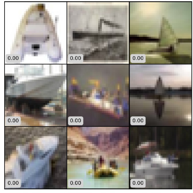
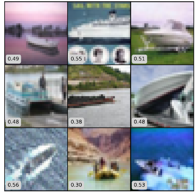
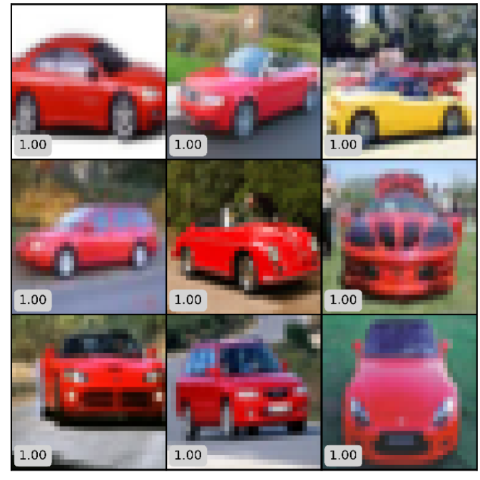
We also present visualizations of images with the highest and lowest pσmmsesubscriptsuperscript𝑝mmse𝜎p^{\mathrm{mmse}}_{\sigma} in each class for each model. For comparison, we do the same with pTsoftmaxsubscriptsuperscript𝑝softmax𝑇p^{\mathrm{softmax}}_{T}. Example CIFAR10 images are shown in the Appendix A.4. We observe that images with low pσrobustsubscriptsuperscript𝑝robust𝜎p^{\mathrm{robust}}_{\sigma} tend to have neutral colors, with the object being a similar color as the background (making the prediction likely to change when the image is slightly perturbed), while images with high pσrobustsubscriptsuperscript𝑝robust𝜎p^{\mathrm{robust}}_{\sigma} tend to be brightly-colored, with the object strongly contrasting with the background (making the prediction likely to stay constant when the image is slightly perturbed). These differences are not as evident for images with the highest and lowest pTsoftmaxsubscriptsuperscript𝑝softmax𝑇p^{\mathrm{softmax}}_{T}. Overall, these results showcase the potential of local robustness in identifying non-robust dataset samples more reliably than softmax probabilities.

5 Conclusion

In this work, we take the first steps towards estimating average-case robustness of multi-class classifiers. Studying average-case robustness provides several advantages over adversarial robustness. First, the nature of real-world noise demands randomized average-case analysis rather than an adversarial one. Second, average-case robustness strictly generalizes adversarial robustness, and therefore provides more information about model behavior than adversarial robustness. Finally, we believe that average-case robustness can offer a gentler objective to train neural networks, when compared to the adversarial case. In particular, requiring models to minimize the probability of misclassification in a local neighborhood is a more lenient objective than attempting to eliminate misclassification entirely as is usually done in adversarial robustness (28).

Future research directions include exploring additional applications of local robustness, such as training average-case robust models that minimize the probability of misclassification and using average-case robustness as a measure of prediction uncertainty.

References

  • Nanda et al. (2021) Vedant Nanda, Samuel Dooley, Sahil Singla, Soheil Feizi, and John P Dickerson. Fairness through robustness: Investigating robustness disparity in deep learning. ACM Conference on Fairness, Accountability, and Transparency, 2021.
  • Carlini and Wagner (2017) Nicholas Carlini and David Wagner. Towards evaluating the robustness of neural networks. IEEE Symposium on Security and Privacy, 2017.
  • Goodfellow et al. (2015) Ian J Goodfellow, Jonathon Shlens, and Christian Szegedy. Explaining and harnessing adversarial examples. International Conference on Learning Representations, 2015.
  • Moosavi-Dezfooli et al. (2016) Seyed-Mohsen Moosavi-Dezfooli, Alhussein Fawzi, and Pascal Frossard. DeepFool: A simple and accurate method to fool deep neural networks. IEEE Conference on Computer Vision and Pattern Recognition, 2016.
  • Cohen et al. (2019) Jeremy Cohen, Elan Rosenfeld, and Zico Kolter. Certified adversarial robustness via randomized smoothing. International Conference on Machine Learning, 2019.
  • Carlini et al. (2022) Nicholas Carlini, Florian Tramer, Krishnamurthy Dvijotham, Leslie Rice, Mingjie Sun, and Zico Kolter. (Certified!!) adversarial robustness for free! International Conference on Learning Representations, 2022.
  • Fazlyab et al. (2019) Mahyar Fazlyab, Manfred Morari, and George J Pappas. Probabilistic verification and reachability analysis of neural networks via semidefinite programming. In 2019 IEEE 58th Conference on Decision and Control (CDC), pages 2726–2731. IEEE, 2019.
  • Kumar et al. (2020) Aounon Kumar, Alexander Levine, Soheil Feizi, and Tom Goldstein. Certifying confidence via randomized smoothing. Advances in Neural Information Processing Systems, 33:5165–5177, 2020.
  • Mangal et al. (2019) Ravi Mangal, Aditya V Nori, and Alessandro Orso. Robustness of neural networks: A probabilistic and practical approach. In 2019 IEEE/ACM 41st International Conference on Software Engineering: New Ideas and Emerging Results (ICSE-NIER), pages 93–96. IEEE, 2019.
  • Franceschi et al. (2018) Jean-Yves Franceschi, Alhussein Fawzi, and Omar Fawzi. Robustness of classifiers to uniform lp and gaussian noise. In International Conference on Artificial Intelligence and Statistics, pages 1280–1288. PMLR, 2018.
  • Robey et al. (2022) Alexander Robey, Luiz Chamon, George J Pappas, and Hamed Hassani. Probabilistically robust learning: Balancing average and worst-case performance. In International Conference on Machine Learning, pages 18667–18686. PMLR, 2022.
  • Rice et al. (2021) Leslie Rice, Anna Bair, Huan Zhang, and J Zico Kolter. Robustness between the worst and average case. Advances in Neural Information Processing Systems, 34:27840–27851, 2021.
  • Weng et al. (2019) Lily Weng, Pin-Yu Chen, Lam Nguyen, Mark Squillante, Akhilan Boopathy, Ivan Oseledets, and Luca Daniel. Proven: Verifying robustness of neural networks with a probabilistic approach. In International Conference on Machine Learning, pages 6727–6736. PMLR, 2019.
  • Vershynin (2018) Roman Vershynin. High-dimensional probability: An introduction with applications in data science. Cambridge University Press, 2018.
  • Pawelczyk et al. (2023) Martin Pawelczyk, Teresa Datta, Johannes van-den Heuvel, Gjergji Kasneci, and Himabindu Lakkaraju. Probabilistically robust recourse: Navigating the trade-offs between costs and robustness in algorithmic recourse. International Conference on Learning Representations, 2023.
  • Botev (2017) Zdravko I Botev. The normal law under linear restrictions: Simulation and estimation via minimax tilting. Journal of the Royal Statistical Society. Series B (Statistical Methodology), 2017.
  • (17) SciPy multivariate normal CDF. https://docs.scipy.org/doc/scipy/reference/generated/scipy.stats.multivariate_normal.html.
  • Patrick (1995) Billingsley Patrick. Probability and measure. A Wiley-Interscience Publication, John Wiley, 118:119, 1995.
  • Srinivas et al. (2022) Suraj Srinivas, Kyle Matoba, Himabindu Lakkaraju, and François Fleuret. Efficient training of low-curvature neural networks. Advances in Neural Information Processing Systems, 35:25951–25964, 2022.
  • Han et al. (2022) Tessa Han, Suraj Srinivas, and Himabindu Lakkaraju. Which explanation should I choose? A function approximation perspective to characterizing post hoc explanations. Neural Information Processing Systems, 2022.
  • Smilkov et al. (2017) Daniel Smilkov, Nikhil Thorat, Been Kim, Fernanda Viégas, and Martin Wattenberg. SmoothGrad: removing noise by adding noise. arXiv preprint arXiv:1706.03825, 2017.
  • Agarwal et al. (2021) Sushant Agarwal, Shahin Jabbari, Chirag Agarwal, Sohini Upadhyay, Steven Wu, and Himabindu Lakkaraju. Towards the unification and robustness of perturbation and gradient based explanations. International Conference on Machine Learning, 2021.
  • Hendrycks and Gimpel (2016) Dan Hendrycks and Kevin Gimpel. Gaussian error linear units (GELUs). arXiv preprint arXiv:1606.08415, 2016.
  • Deng (2012) Li Deng. The MNIST database of handwritten digit images for machine learning research. IEEE Signal Processing Magazine, 2012.
  • Xiao et al. (2017) Han Xiao, Kashif Rasul, and Roland Vollgraf. Fashion-MNIST: A novel image dataset for benchmarking machine learning algorithms. arXiv preprint arXiv:1708.07747, 2017.
  • Krizhevsky et al. (2009) Alex Krizhevsky, Geoffrey Hinton, et al. Learning multiple layers of features from tiny images. University of Toronto, 2009.
  • He et al. (2016) Kaiming He, Xiangyu Zhang, Shaoqing Ren, and Jian Sun. Deep residual learning for image recognition. IEEE Conference on Computer Vision and Pattern Recognition, 2016.
  • Croce et al. (2021) Francesco Croce, Maksym Andriushchenko, Vikash Sehwag, Edoardo Debenedetti, Nicolas Flammarion, Mung Chiang, Prateek Mittal, and Matthias Hein. Robustbench: a standardized adversarial robustness benchmark. In Thirty-fifth Conference on Neural Information Processing Systems Datasets and Benchmarks Track (Round 2), 2021.

Appendix A Appendix

A.1 Proofs

Lemma A.1.

The local robustness of a multi-class linear model f(𝐱)=𝐰𝐱+b𝑓𝐱superscript𝐰top𝐱𝑏f(\mathbf{x})=\mathbf{w}^{\top}\mathbf{x}+b (with 𝐰d×C𝐰superscript𝑑𝐶\mathbf{w}\in\mathbb{R}^{d\times C} and bC𝑏superscript𝐶b\in\mathbb{R}^{C}) at point 𝐱𝐱\mathbf{x} with respect to a target class t𝑡t is given by the following. Define weights 𝐮i=𝐰t𝐰id,itformulae-sequencesubscript𝐮𝑖subscript𝐰𝑡subscript𝐰𝑖superscript𝑑for-all𝑖𝑡\mathbf{u}_{i}=\mathbf{w}_{t}-\mathbf{w}_{i}\in\mathbb{R}^{d},\forall i\neq t, where 𝐰t,𝐰isubscript𝐰𝑡subscript𝐰𝑖\mathbf{w}_{t},\mathbf{w}_{i} are rows of 𝐰𝐰\mathbf{w} and biases ci=𝐮i𝐱+(btbi)subscript𝑐𝑖superscriptsubscript𝐮𝑖top𝐱subscript𝑏𝑡subscript𝑏𝑖c_{i}={\mathbf{u}_{i}}^{\top}\mathbf{x}+(b_{t}-b_{i})\in\mathbb{R}. Then,

pσrobust(𝐱)=Φ𝐔𝐔(ciσ𝐮i2|i=1itC)subscriptsuperscript𝑝robust𝜎𝐱subscriptΦsuperscript𝐔𝐔topevaluated-atsubscript𝑐𝑖𝜎subscriptnormsubscript𝐮𝑖2𝑖1𝑖𝑡𝐶\displaystyle p^{\text{robust}}_{\sigma}(\mathbf{x})=\Phi_{\mathbf{U}\mathbf{U}^{\top}}\left(\frac{c_{i}}{\sigma\|\mathbf{u}_{i}\|_{2}}~{}\bigg{|}_{\begin{subarray}{c}i=1\\ i\neq t\end{subarray}}^{C}\right)
where𝐔=𝐮i𝐮i2|i=1itC(C1)×dwhere𝐔evaluated-atsubscript𝐮𝑖subscriptnormsubscript𝐮𝑖2𝑖1𝑖𝑡𝐶superscript𝐶1𝑑\displaystyle\mathrm{where}~{}~{}\mathbf{U}=\frac{\mathbf{u}_{i}}{\|\mathbf{u}_{i}\|_{2}}~{}\bigg{|}_{\begin{subarray}{c}i=1\\ i\neq t\end{subarray}}^{C}\in\mathbb{R}^{(C-1)\times d}

and Φ𝐔𝐔subscriptΦsuperscript𝐔𝐔top\Phi_{\mathbf{U}\mathbf{U}^{\top}} is the (C1𝐶1C-1)-dimensional Normal CDF with zero mean and covariance 𝐔𝐔superscript𝐔𝐔top\mathbf{U}\mathbf{U}^{\top}.

Proof.

First, we rewrite pσrobustsubscriptsuperscript𝑝robust𝜎p^{\mathrm{robust}}_{\sigma} in the following manner, by defining gi(𝐱)=ft(𝐱)fi(𝐱)>0subscript𝑔𝑖𝐱subscript𝑓𝑡𝐱subscript𝑓𝑖𝐱0g_{i}(\mathbf{x})=f_{t}(\mathbf{x})-f_{i}(\mathbf{x})>0, which is the “decision boundary function".

pσrobust=Pϵ𝒩(0,σ2)[maxifi(𝐱+ϵ)<ft(𝐱+ϵ)]superscriptsubscript𝑝𝜎robustsubscript𝑃similar-toitalic-ϵ𝒩0superscript𝜎2delimited-[]subscript𝑖subscript𝑓𝑖𝐱italic-ϵsubscript𝑓𝑡𝐱italic-ϵ\displaystyle p_{\sigma}^{\text{robust}}=P_{\epsilon\sim\mathcal{N}(0,\sigma^{2})}\left[\max_{i}f_{i}(\mathbf{x}+\epsilon)<f_{t}(\mathbf{x}+\epsilon)\right]
=Pϵ𝒩(0,σ2)[i=1;itCgi(𝐱+ϵ)>0]absentsubscript𝑃similar-toitalic-ϵ𝒩0superscript𝜎2delimited-[]superscriptsubscriptformulae-sequence𝑖1𝑖𝑡𝐶subscript𝑔𝑖𝐱italic-ϵ0\displaystyle=P_{\epsilon\sim\mathcal{N}(0,\sigma^{2})}\left[\bigcup_{i=1;i\neq t}^{C}g_{i}(\mathbf{x}+\epsilon)>0\right]

Now, assuming that f,g𝑓𝑔f,g are linear such that gi(𝐱)=𝐮i𝐱+g(0)subscript𝑔𝑖𝐱superscriptsubscriptsuperscript𝐮𝑖top𝐱𝑔0g_{i}(\mathbf{x})={\mathbf{u}^{\prime}_{i}}^{\top}\mathbf{x}+g(0), we have gi(𝐱+ϵ)=gi(𝐱)+𝐮iϵsubscript𝑔𝑖𝐱italic-ϵsubscript𝑔𝑖𝐱superscriptsubscript𝐮𝑖topitalic-ϵg_{i}(\mathbf{x}+\epsilon)=g_{i}(\mathbf{x})+{\mathbf{u}_{i}}^{\top}\epsilon, and obtain

pσrobustsuperscriptsubscript𝑝𝜎robust\displaystyle p_{\sigma}^{\text{robust}} =Pϵ𝒩(0,σ2)[i=1;itC𝐮iϵ>gi(𝐱)]absentsubscript𝑃similar-toitalic-ϵ𝒩0superscript𝜎2delimited-[]superscriptsubscriptformulae-sequence𝑖1𝑖𝑡𝐶superscriptsubscript𝐮𝑖topitalic-ϵsubscript𝑔𝑖𝐱\displaystyle=P_{\epsilon\sim\mathcal{N}(0,\sigma^{2})}\left[\bigcup_{i=1;i\neq t}^{C}{\mathbf{u}_{i}}^{\top}\epsilon>-g_{i}(\mathbf{x})\right] (1)
=Pz𝒩(0,Id)[i=1;itC𝐮i𝐮i2z>gi(𝐱)σ𝐮i2]absentsubscript𝑃similar-to𝑧𝒩0subscript𝐼𝑑delimited-[]superscriptsubscriptformulae-sequence𝑖1𝑖𝑡𝐶superscriptsubscript𝐮𝑖subscriptnormsubscript𝐮𝑖2top𝑧subscript𝑔𝑖𝐱𝜎subscriptnormsubscript𝐮𝑖2\displaystyle=P_{z\sim\mathcal{N}(0,I_{d})}\left[\bigcup_{i=1;i\neq t}^{C}\frac{\mathbf{u}_{i}}{\|\mathbf{u}_{i}\|_{2}}^{\top}z>-\frac{g_{i}(\mathbf{x})}{\sigma\|\mathbf{u}_{i}\|_{2}}\right] (2)

This step simply involves rescaling and standardizing the Gaussian to be unit normal. We now make the following observations:

  • For any matrix 𝐔C1×d𝐔superscript𝐶1𝑑\mathbf{U}\in\mathbb{R}^{C-1\times d} and a d-dimensional Gaussian random variable z𝒩(0,Id)dsimilar-to𝑧𝒩0subscript𝐼𝑑superscript𝑑z\sim\mathcal{N}(0,I_{d})\in\mathbb{R}^{d}, we have 𝐔z𝒩(0,𝐔𝐔)similar-tosuperscript𝐔top𝑧𝒩0superscript𝐔𝐔top\mathbf{U}^{\top}z\sim\mathcal{N}(0,\mathbf{U}\mathbf{U}^{\top}), i.e., an (C-1) -dimensional Gaussian random variable.

  • CDF of a multivariate Gaussian RV is defined as Pz[izi<ti]subscript𝑃𝑧delimited-[]subscript𝑖subscript𝑧𝑖subscript𝑡𝑖P_{z}[\bigcup_{i}z_{i}<t_{i}] for some input values tisubscript𝑡𝑖t_{i}

Using these observations, if we construct 𝐔=𝐮i𝐮i2|i=1itC(C1)×d𝐔evaluated-atsubscript𝐮𝑖subscriptnormsubscript𝐮𝑖2𝑖1𝑖𝑡𝐶superscript𝐶1𝑑\mathbf{U}=\frac{\mathbf{u}_{i}}{\|\mathbf{u}_{i}\|_{2}}~{}\bigg{|}_{\begin{subarray}{c}i=1\\ i\neq t\end{subarray}}^{C}\in\mathbb{R}^{(C-1)\times d}, and obtain

pσrobustsubscriptsuperscript𝑝robust𝜎\displaystyle p^{\text{robust}}_{\sigma} =Pr𝒩(0,𝐔𝐔)[i=1;itCri<gi(𝐱)σ𝐮i2]absentsubscript𝑃similar-to𝑟𝒩0superscript𝐔𝐔topdelimited-[]superscriptsubscriptformulae-sequence𝑖1𝑖𝑡𝐶subscript𝑟𝑖subscript𝑔𝑖𝐱𝜎subscriptnormsubscript𝐮𝑖2\displaystyle=P_{r\sim\mathcal{N}(0,\mathbf{U}\mathbf{U}^{\top})}\left[\bigcup_{i=1;i\neq t}^{C}r_{i}<\frac{g_{i}(\mathbf{x})}{\sigma\|\mathbf{u}_{i}\|_{2}}\right]
=CDF𝒩(0,UU)(gi(𝐱)σ𝐮i2|i=1itC)absentsubscriptCDF𝒩0𝑈superscript𝑈topevaluated-atsubscript𝑔𝑖𝐱𝜎subscriptnormsubscript𝐮𝑖2𝑖1𝑖𝑡𝐶\displaystyle=\text{CDF}_{\mathcal{N}(0,UU^{\top})}\left(\frac{g_{i}(\mathbf{x})}{\sigma\|\mathbf{u}_{i}\|_{2}}~{}\bigg{|}_{\begin{subarray}{c}i=1\\ i\neq t\end{subarray}}^{C}\right)

where gi(𝐱)=𝐮i𝐱+gi(0)=(𝐰t𝐰i)𝐱+(btbi)subscript𝑔𝑖𝐱superscriptsubscript𝐮𝑖top𝐱subscript𝑔𝑖0superscriptsubscript𝐰𝑡subscript𝐰𝑖top𝐱subscript𝑏𝑡subscript𝑏𝑖g_{i}(\mathbf{x})={\mathbf{u}_{i}}^{\top}\mathbf{x}+g_{i}(0)={(\mathbf{w}_{t}-\mathbf{w}_{i})}^{\top}\mathbf{x}+(b_{t}-b_{i})

Lemma A.2.

(Extension to non-Gaussian noise) For high-dimensional data (d𝑑d\rightarrow\infty), Lemma 3.1 generalizes to any coordinate-wise independent noise distribution that satisfies Lyapunov’s condition.

Proof.

Applying Lyupanov’s central limit theorem, given ϵsimilar-toitalic-ϵ\epsilon\sim\mathcal{R} is sampled from some distribution \mathcal{R} to equation 2 in the previous proof, we have we have 𝐮σ𝐮2ϵ=j=1d𝐮jσ𝐮2ϵjd𝒩(0,1)superscript𝐮𝜎subscriptnorm𝐮2topitalic-ϵsuperscriptsubscript𝑗1𝑑subscript𝐮𝑗𝜎subscriptnorm𝐮2subscriptitalic-ϵ𝑗𝑑𝒩01\frac{\mathbf{u}}{\sigma\|\mathbf{u}\|_{2}}^{\top}\epsilon=\sum_{j=1}^{d}\frac{\mathbf{u}_{j}}{\sigma\|\mathbf{u}\|_{2}}\epsilon_{j}~{}~{}\begin{subarray}{c}d\\ \longrightarrow\end{subarray}~{}~{}\mathcal{N}(0,1), which holds as long as the sequence {𝐮j𝐮2ϵj}subscript𝐮𝑗subscriptnorm𝐮2subscriptitalic-ϵ𝑗\{\frac{\mathbf{u}_{j}}{\|\mathbf{u}\|_{2}}\epsilon_{j}\} are independent random variables and satisfy the Lyapunov condition. In particular, this implies that 𝐔z𝒩(0,𝐔𝐔)similar-tosuperscript𝐔top𝑧𝒩0superscript𝐔𝐔top\mathbf{U}^{\top}z\sim\mathcal{N}(0,\mathbf{U}\mathbf{U}^{\top}), and the proof proceeds as similar to the Gaussian case after this step. ∎

Lemma A.3.

(Extension to non-isotropic Gaussian) Lemma 3.1 can be extended to the case of ϵ𝒩(0,𝒞)similar-toitalic-ϵ𝒩0𝒞\epsilon\sim\mathcal{N}(0,\mathcal{C}) for an arbitrary positive definite covariance matrix 𝒞𝒞\mathcal{C}:

pσrobust(𝐱)=Φ𝐔𝒞𝐔(ci𝐮i2|i=1itC)subscriptsuperscript𝑝robust𝜎𝐱subscriptΦ𝐔𝒞superscript𝐔topevaluated-atsubscript𝑐𝑖subscriptnormsubscript𝐮𝑖2𝑖1𝑖𝑡𝐶\displaystyle p^{\text{robust}}_{\sigma}(\mathbf{x})=\Phi_{\mathbf{U}\mathcal{C}\mathbf{U}^{\top}}\left(\frac{c_{i}}{\|\mathbf{u}_{i}\|_{2}}~{}\bigg{|}_{\begin{subarray}{c}i=1\\ i\neq t\end{subarray}}^{C}\right)
Proof.

We observe that the Gaussian random variable 𝐮i𝐮iϵ|i=1ttC=𝐔ϵevaluated-atsuperscriptsubscript𝐮𝑖normsubscript𝐮𝑖topitalic-ϵ𝑖1𝑡𝑡𝐶superscript𝐔topitalic-ϵ\frac{\mathbf{u}_{i}}{\|\mathbf{u}_{i}\|}^{\top}\epsilon|_{\begin{subarray}{c}i=1\\ t\neq t\end{subarray}}^{C}=\mathbf{U}^{\top}\epsilon has mean zero as ϵitalic-ϵ\epsilon is mean zero. Computing its covariance matrix, we have 𝔼ϵ𝐔ϵϵ𝐔=𝐔𝔼ϵ(ϵϵ)𝐔=𝐔𝒞𝐔subscript𝔼italic-ϵsuperscript𝐔topitalic-ϵsuperscriptitalic-ϵtop𝐔superscript𝐔topsubscript𝔼italic-ϵitalic-ϵsuperscriptitalic-ϵtop𝐔superscript𝐔top𝒞𝐔\mathop{\mathbb{E}}_{\epsilon}\mathbf{U}^{\top}\epsilon\epsilon^{\top}\mathbf{U}=\mathbf{U}^{\top}\mathop{\mathbb{E}}_{\epsilon}(\epsilon\epsilon^{\top})\mathbf{U}=\mathbf{U}^{\top}\mathcal{C}\mathbf{U}. We use this result after equation 2 in the proof of Lemma 3.1. ∎

Proposition A.1.

The Taylor estimator for the local robustness of a classifier f𝑓f at point 𝐱𝐱\mathbf{x} with respect to target class t𝑡t is given by linearizing f𝑓f around 𝐱𝐱\mathbf{x} using a first-order Taylor expansion, with decision boundaries gi(𝐱)=ft(𝐱)fi(𝐱)subscript𝑔𝑖𝐱subscript𝑓𝑡𝐱subscript𝑓𝑖𝐱g_{i}(\mathbf{x})=f_{t}(\mathbf{x})-f_{i}(\mathbf{x}), itfor-all𝑖𝑡\forall i\neq t, leading to

pσtaylor(𝐱)=Φ𝐔𝐔(gi(𝐱)σ𝐱gi(𝐱)2|i=1itC)subscriptsuperscript𝑝taylor𝜎𝐱subscriptΦsuperscript𝐔𝐔topevaluated-atsubscript𝑔𝑖𝐱𝜎subscriptnormsubscript𝐱subscript𝑔𝑖𝐱2𝑖1𝑖𝑡𝐶\displaystyle p^{\text{taylor}}_{\sigma}(\mathbf{x})=\Phi_{\mathbf{U}\mathbf{U}^{\top}}\left(\frac{g_{i}(\mathbf{x})}{\sigma\|\nabla_{\mathbf{x}}g_{i}(\mathbf{x})\|_{2}}~{}\bigg{|}_{\begin{subarray}{c}i=1\\ i\neq t\end{subarray}}^{C}\right)

with 𝐔𝐔\mathbf{U} and ΦΦ\Phi defined as in the linear case.

Proof.

Using the notations from the previous Lemma A.1, we can linearize g(𝐱+ϵ)g(𝐱)+𝐱g(𝐱)ϵ𝑔𝐱italic-ϵ𝑔𝐱subscript𝐱𝑔superscript𝐱topitalic-ϵg(\mathbf{x}+\epsilon)\approx g(\mathbf{x})+\nabla_{\mathbf{x}}g(\mathbf{x})^{\top}\epsilon using a first order Taylor series expansion. Thus we use 𝐮i=𝐱gi(𝐱)subscript𝐮𝑖subscript𝐱subscript𝑔𝑖𝐱\mathbf{u}_{i}=\nabla_{\mathbf{x}}g_{i}(\mathbf{x}) and ci=gi(𝐱)subscript𝑐𝑖subscript𝑔𝑖𝐱c_{i}=g_{i}(\mathbf{x}), and plug it into the result of Lemma A.1. ∎

Proposition A.2.

The estimation error of the Taylor estimator for a classifier with a quadratic decision boundary gi(𝐱)=𝐱Ai𝐱+𝐮i𝐱+cisubscript𝑔𝑖𝐱superscript𝐱topsubscript𝐴𝑖𝐱superscriptsubscript𝐮𝑖top𝐱subscript𝑐𝑖g_{i}(\mathbf{x})=\mathbf{x}^{\top}A_{i}\mathbf{x}+\mathbf{u}_{i}^{\top}\mathbf{x}+c_{i} for positive-definite Aisubscript𝐴𝑖A_{i}, is upper bounded by

|pσrobust(𝐱)pσtaylor(𝐱)|kσC1i=1itCλmaxAi𝐮i2subscriptsuperscript𝑝𝑟𝑜𝑏𝑢𝑠𝑡𝜎𝐱subscriptsuperscript𝑝𝑡𝑎𝑦𝑙𝑜𝑟𝜎𝐱𝑘superscript𝜎𝐶1superscriptsubscriptproduct𝑖1𝑖𝑡𝐶superscriptsubscript𝜆subscript𝐴𝑖subscriptnormsubscript𝐮𝑖2\displaystyle|p^{robust}_{\sigma}(\mathbf{x})-p^{taylor}_{\sigma}(\mathbf{x})|\leq k\sigma^{C-1}\prod_{\begin{subarray}{c}i=1\\ i\neq t\end{subarray}}^{C}\frac{\lambda_{\max}^{A_{i}}}{\|\mathbf{u}_{i}\|_{2}}

for noise ϵ𝒩(0,σ2/d)similar-toitalic-ϵ𝒩0superscript𝜎2𝑑\epsilon\sim\mathcal{N}(0,\sigma^{2}/d), in the limit of d𝑑d\rightarrow\infty.

Proof.

Without loss of generality, assume that 𝐱=0𝐱0\mathbf{x}=0. For any other 𝐱10subscript𝐱10\mathbf{x}_{1}\neq 0, we can simply perform a change of variables of the underlying function to center it at 𝐱1subscript𝐱1\mathbf{x}_{1} to yield a different quadratic. We first write an expression for pσrobustsubscriptsuperscript𝑝𝑟𝑜𝑏𝑢𝑠𝑡𝜎p^{robust}_{\sigma} for the given quadratic classifier gi(𝐱)subscript𝑔𝑖𝐱g_{i}(\mathbf{x}) at 𝐱=0𝐱0\mathbf{x}=0.

pσrobust(0)subscriptsuperscript𝑝𝑟𝑜𝑏𝑢𝑠𝑡𝜎0\displaystyle p^{robust}_{\sigma}(0) =Pϵ(igi(ϵ)>0)absentsubscript𝑃italic-ϵsubscript𝑖subscript𝑔𝑖italic-ϵ0\displaystyle=P_{\epsilon}\left(\bigcup_{i}g_{i}(\epsilon)>0\right)
=Pϵ(i𝐮iϵ+c>ϵAiϵ)absentsubscript𝑃italic-ϵsubscript𝑖superscriptsubscript𝐮𝑖topitalic-ϵ𝑐superscriptitalic-ϵtopsubscript𝐴𝑖italic-ϵ\displaystyle=P_{\epsilon}\left(\bigcup_{i}\mathbf{u}_{i}^{\top}\epsilon+c>-\epsilon^{\top}A_{i}\epsilon\right)

Similarly, computing, pσtaylorsubscriptsuperscript𝑝𝑡𝑎𝑦𝑙𝑜𝑟𝜎p^{taylor}_{\sigma} we have 𝐱gi(0)=𝐮subscript𝐱subscript𝑔𝑖0superscript𝐮top\nabla_{\mathbf{x}}g_{i}(0)=\mathbf{u}^{\top} and gi(0)=cisubscript𝑔𝑖0subscript𝑐𝑖g_{i}(0)=c_{i}, resulting in

pσtaylor(0)subscriptsuperscript𝑝𝑡𝑎𝑦𝑙𝑜𝑟𝜎0\displaystyle p^{taylor}_{\sigma}(0) =Pϵ(igitaylor(ϵ)>0)absentsubscript𝑃italic-ϵsubscript𝑖subscriptsuperscript𝑔𝑡𝑎𝑦𝑙𝑜𝑟𝑖italic-ϵ0\displaystyle=P_{\epsilon}\left(\bigcup_{i}g^{taylor}_{i}(\epsilon)>0\right)
=Pϵ(i𝐮iϵ+c>0)absentsubscript𝑃italic-ϵsubscript𝑖superscriptsubscript𝐮𝑖topitalic-ϵ𝑐0\displaystyle=P_{\epsilon}\left(\bigcup_{i}\mathbf{u}_{i}^{\top}\epsilon+c>0\right)

Subtracting the two, we have

|pσrobust(0)pσtaylor(0)|subscriptsuperscript𝑝𝑟𝑜𝑏𝑢𝑠𝑡𝜎0subscriptsuperscript𝑝𝑡𝑎𝑦𝑙𝑜𝑟𝜎0\displaystyle|p^{robust}_{\sigma}(0)-p^{taylor}_{\sigma}(0)|
=|P(i0>𝐮iϵ+c>ϵAiϵ)|absent𝑃subscript𝑖0superscriptsubscript𝐮𝑖topitalic-ϵ𝑐superscriptitalic-ϵtopsubscript𝐴𝑖italic-ϵ\displaystyle=\left|P\left(\bigcup_{i}0>\mathbf{u}_{i}^{\top}\epsilon+c>-\epsilon^{\top}A_{i}\epsilon\right)\right|
=|P(i0>𝐮iϵ+cσ𝐮i2>ϵAiϵσ𝐮i2)|absent𝑃subscript𝑖0superscriptsubscript𝐮𝑖topitalic-ϵ𝑐𝜎subscriptnormsubscript𝐮𝑖2superscriptitalic-ϵtopsubscript𝐴𝑖italic-ϵ𝜎subscriptnormsubscript𝐮𝑖2\displaystyle=\left|P\left(\bigcup_{i}0>\frac{\mathbf{u}_{i}^{\top}\epsilon+c}{\sigma\|\mathbf{u}_{i}\|_{2}}>-\frac{\epsilon^{\top}A_{i}\epsilon}{\sigma\|\mathbf{u}_{i}\|_{2}}\right)\right|

For high-dimensional Gaussian noise ϵ𝒩(0,σ2/d)similar-toitalic-ϵ𝒩0superscript𝜎2𝑑\epsilon\sim\mathcal{N}(0,\sigma^{2}/d), with d𝑑d\rightarrow\infty, we have that ϵ2=iϵi2σ2superscriptnormitalic-ϵ2subscript𝑖superscriptsubscriptitalic-ϵ𝑖2superscript𝜎2\|\epsilon\|^{2}=\sum_{i}\epsilon_{i}^{2}\rightarrow\sigma^{2} from the law of large numbers. See (14) for an extended discussion. Thus we have ϵAϵλmaxAϵ2=λmaxAσ2superscriptitalic-ϵtop𝐴italic-ϵsuperscriptsubscript𝜆𝐴superscriptnormitalic-ϵ2superscriptsubscript𝜆𝐴superscript𝜎2\epsilon^{\top}A\epsilon\leq\lambda_{\max}^{A}\|\epsilon\|^{2}=\lambda_{\max}^{A}\sigma^{2}.

Also let zi=𝐮iϵ+cσ𝐮i2subscript𝑧𝑖superscriptsubscript𝐮𝑖topitalic-ϵ𝑐𝜎subscriptnormsubscript𝐮𝑖2z_{i}=\frac{\mathbf{u}_{i}^{\top}\epsilon+c}{\sigma\|\mathbf{u}_{i}\|_{2}} be a random variable. We observe that zi|ievaluated-atsubscript𝑧𝑖𝑖z_{i}|_{i} is a tensor extension of zisubscript𝑧𝑖z_{i}, has a covariance matrix of 𝐔𝐔superscript𝐔𝐔top\mathbf{U}\mathbf{U}^{\top} as before. Let us also define 𝒞i=λmaxAi𝐮i2subscript𝒞𝑖superscriptsubscript𝜆subscript𝐴𝑖subscriptnormsubscript𝐮𝑖2\mathcal{C}_{i}=\frac{\lambda_{\max}^{A_{i}}}{\|\mathbf{u}_{i}\|_{2}}.

||\displaystyle| pσrobust(0)pσtaylor(0)|\displaystyle p^{robust}_{\sigma}(0)-p^{taylor}_{\sigma}(0)|
=|P(i0>zi(ϵ)>ϵAiϵσ𝐮i2)|absent𝑃subscript𝑖0subscript𝑧𝑖italic-ϵsuperscriptitalic-ϵtopsubscript𝐴𝑖italic-ϵ𝜎subscriptnormsubscript𝐮𝑖2\displaystyle=\left|P\left(\bigcup_{i}0>z_{i}(\epsilon)>-\frac{\epsilon^{\top}A_{i}\epsilon}{\sigma\|\mathbf{u}_{i}\|_{2}}\right)\right|
|P(i0>zi>λmaxAi𝐮i2σ)|(ϵAϵ<λmaxAσ2)absent𝑃subscript𝑖0subscript𝑧𝑖superscriptsubscript𝜆subscript𝐴𝑖subscriptnormsubscript𝐮𝑖2𝜎superscriptitalic-ϵtop𝐴italic-ϵsuperscriptsubscript𝜆𝐴superscript𝜎2\displaystyle\leq\left|P\left(\bigcup_{i}0>z_{i}>-\frac{\lambda_{\max}^{A_{i}}}{\|\mathbf{u}_{i}\|_{2}}\sigma\right)\right|~{}~{}~{}(\epsilon^{\top}A\epsilon<\lambda_{\max}^{A}\sigma^{2})
=|𝒞iσ0pdf(zi|i)dzi|i|(Defn of mvn cdf)\displaystyle=\left|\int...\int^{0}_{-\mathcal{C}_{i}\sigma}\text{pdf}(z_{i}|_{i})~{}\mathrm{d}z_{i}|_{i}\right|~{}~{}~{}(\text{Defn of mvn cdf})
maxzi|ipdf(zi|i)i|Ciσ|(Upper bound pdf with its max)absentsubscriptevaluated-atsubscript𝑧𝑖𝑖pdfevaluated-atsubscript𝑧𝑖𝑖subscriptproduct𝑖subscript𝐶𝑖𝜎Upper bound pdf with its max\displaystyle\leq\max_{z_{i}|_{i}}\text{pdf}(z_{i}|_{i})~{}\prod_{i}|C_{i}\sigma|~{}~{}~{}(\text{Upper bound pdf with its max})
(2π)(C1)/2det(𝐔𝐔)1/2i=1itCCiσabsentsuperscript2𝜋𝐶12superscriptsuperscript𝐔𝐔top12superscriptsubscriptproduct𝑖1𝑖𝑡𝐶subscript𝐶𝑖𝜎\displaystyle\leq(2\pi)^{-(C-1)/2}\det(\mathbf{U}\mathbf{U}^{\top})^{-1/2}\prod_{\begin{subarray}{c}i=1\\ i\neq t\end{subarray}}^{C}C_{i}\sigma
=k(σC1i=1itCλmaxAi𝐮i2)absent𝑘superscript𝜎𝐶1superscriptsubscriptproduct𝑖1𝑖𝑡𝐶superscriptsubscript𝜆subscript𝐴𝑖subscriptnormsubscript𝐮𝑖2\displaystyle=k\left(\sigma^{C-1}\prod_{\begin{subarray}{c}i=1\\ i\neq t\end{subarray}}^{C}\frac{\lambda_{\max}^{A_{i}}}{\|\mathbf{u}_{i}\|_{2}}\right)

where k=maxzpdf(z)=(2π)(C1)/2det(𝐔𝐔)1/2𝑘subscript𝑧𝑝𝑑𝑓𝑧superscript2𝜋𝐶12superscriptsuperscript𝐔𝐔top12k=\max_{z}pdf(z)=(2\pi)^{-(C-1)/2}\det(\mathbf{U}\mathbf{U}^{\top})^{-1/2}, which is the max value of the Gaussian pdf. Note that as the rows of 𝐔𝐔\mathbf{U} are normalized, det(𝐔)1𝐔1\det(\mathbf{U})\leq 1 and det(𝐔𝐔)=det(𝐔)21superscript𝐔𝐔topsuperscript𝐔21\det(\mathbf{U}\mathbf{U}^{\top})=\det(\mathbf{U})^{2}\leq 1.

We note that these bounds are rather pessimistic, as in high-dimensions ϵAiϵλmeanAiλmaxAisimilar-tosuperscriptitalic-ϵtopsubscript𝐴𝑖italic-ϵsuperscriptsubscript𝜆meansubscript𝐴𝑖superscriptsubscript𝜆subscript𝐴𝑖\epsilon^{\top}A_{i}\epsilon\sim\lambda_{\text{mean}}^{A_{i}}\leq\lambda_{\max}^{A_{i}}, and thus in reality the errors are expected to be much smaller.

Proposition A.3.

The MMSE estimator for the local robustness of a classifier f𝑓f at point 𝐱𝐱\mathbf{x} with respect to target class t𝑡t is given by an MMSE linearization f𝑓f around 𝐱𝐱\mathbf{x}, for decision boundaries gi(𝐱)=ft(𝐱)fi(𝐱)subscript𝑔𝑖𝐱subscript𝑓𝑡𝐱subscript𝑓𝑖𝐱g_{i}(\mathbf{x})=f_{t}(\mathbf{x})-f_{i}(\mathbf{x}), itfor-all𝑖𝑡\forall i\neq t, leading to

pσmmse(𝐱)=Φ𝐔𝐔(g~i(𝐱)σ𝐱g~i(𝐱)2|i=1itC)subscriptsuperscript𝑝mmse𝜎𝐱subscriptΦsuperscript𝐔𝐔topevaluated-atsubscript~𝑔𝑖𝐱𝜎subscriptnormsubscript𝐱subscript~𝑔𝑖𝐱2𝑖1𝑖𝑡𝐶\displaystyle p^{\text{mmse}}_{\sigma}(\mathbf{x})=\Phi_{\mathbf{U}\mathbf{U}^{\top}}\left(\frac{\tilde{g}_{i}(\mathbf{x})}{\sigma\|\nabla_{\mathbf{x}}\tilde{g}_{i}(\mathbf{x})\|_{2}}~{}\bigg{|}_{\begin{subarray}{c}i=1\\ i\neq t\end{subarray}}^{C}\right)
whereg~i(𝐱)=1Nj=1Ngi(𝐱+ϵ),ϵ𝒩(0,σ2)formulae-sequencewheresubscript~𝑔𝑖𝐱1𝑁superscriptsubscript𝑗1𝑁subscript𝑔𝑖𝐱italic-ϵsimilar-toitalic-ϵ𝒩0superscript𝜎2\displaystyle\mathrm{where}~{}~{}\tilde{g}_{i}(\mathbf{x})=\frac{1}{N}\sum_{j=1}^{N}g_{i}(\mathbf{x}+\epsilon)~{},~{}\epsilon\sim\mathcal{N}(0,\sigma^{2})

with 𝐔𝐔\mathbf{U} and ΦΦ\Phi defined as in the linear case, and N𝑁N is the number of perturbations.

Proof.

We would like to improve upon the Taylor approximation to g(𝐱+ϵ)𝑔𝐱italic-ϵg(\mathbf{x}+\epsilon) by using an MMSE local function approximation. Essentially, we’d like the find 𝐮d𝐮superscript𝑑\mathbf{u}\in\mathbb{R}^{d} and c𝑐c\in\mathbb{R} such that

(𝐮(𝐱),c(𝐱))=argmin𝐮,c𝔼ϵ𝒩(0,σ2)(g(x+ϵ)𝐮ϵc)2superscript𝐮𝐱superscript𝑐𝐱subscript𝐮𝑐subscript𝔼similar-toitalic-ϵ𝒩0superscript𝜎2superscript𝑔𝑥italic-ϵsuperscript𝐮topitalic-ϵ𝑐2\displaystyle(\mathbf{u}^{*}(\mathbf{x}),c^{*}(\mathbf{x}))=\arg\min_{\mathbf{u},c}\mathop{\mathbb{E}}_{\epsilon\sim\mathcal{N}(0,\sigma^{2})}(g(x+\epsilon)-\mathbf{u}^{\top}\epsilon-c)^{2}

A straightforward solution by finding critical points and equating it to zero gives us the following:

𝐮(𝐱)superscript𝐮𝐱\displaystyle\mathbf{u}^{*}(\mathbf{x}) =𝔼ϵ[g(x+ϵ)ϵ]/σ2absentsubscript𝔼italic-ϵdelimited-[]𝑔𝑥italic-ϵsuperscriptitalic-ϵtopsuperscript𝜎2\displaystyle=\mathop{\mathbb{E}}_{\epsilon}\left[g(x+\epsilon)\epsilon^{\top}\right]/\sigma^{2}
=𝔼ϵ[𝐱g(𝐱+ϵ)](Stein’s Lemma)absentsubscript𝔼italic-ϵdelimited-[]subscript𝐱𝑔𝐱italic-ϵStein’s Lemma\displaystyle=\mathop{\mathbb{E}}_{\epsilon}\left[\nabla_{\mathbf{x}}g(\mathbf{x}+\epsilon)\right]~{}~{}~{}~{}~{}(\text{Stein's Lemma})
c(𝐱)superscript𝑐𝐱\displaystyle c^{*}(\mathbf{x}) =𝔼ϵg(x+ϵ)absentsubscript𝔼italic-ϵ𝑔𝑥italic-ϵ\displaystyle=\mathop{\mathbb{E}}_{\epsilon}g(x+\epsilon)

Plugging in these values of U,csuperscript𝑈superscript𝑐U^{*},c^{*} into Lemma A.1, we have the result.

Proposition A.4.

The estimation error of the MMSE estimator for a classifier with a quadratic decision boundary g(𝐱)=𝐱A𝐱+𝐮𝐱+c𝑔𝐱superscript𝐱top𝐴𝐱superscript𝐮top𝐱𝑐g(\mathbf{x})=\mathbf{x}^{\top}A\mathbf{x}+\mathbf{u}^{\top}\mathbf{x}+c, and positive definite A𝐴A is upper bounded by

|pσrobust(𝐱)pσmmse(𝐱)|kσC1i=1itC|λmaxAiλmeanAi|𝐮i2subscriptsuperscript𝑝𝑟𝑜𝑏𝑢𝑠𝑡𝜎𝐱subscriptsuperscript𝑝𝑚𝑚𝑠𝑒𝜎𝐱𝑘superscript𝜎𝐶1superscriptsubscriptproduct𝑖1𝑖𝑡𝐶superscriptsubscript𝜆subscript𝐴𝑖superscriptsubscript𝜆meansubscript𝐴𝑖subscriptnormsubscript𝐮𝑖2\displaystyle|p^{robust}_{\sigma}(\mathbf{x})-p^{mmse}_{\sigma}(\mathbf{x})|\leq k\sigma^{C-1}\prod_{\begin{subarray}{c}i=1\\ i\neq t\end{subarray}}^{C}\frac{|\lambda_{\max}^{A_{i}}-\lambda_{\mathrm{mean}}^{A_{i}}|}{\|\mathbf{u}_{i}\|_{2}}

for noise ϵ𝒩(0,σ2/d)similar-toitalic-ϵ𝒩0superscript𝜎2𝑑\epsilon\sim\mathcal{N}(0,\sigma^{2}/d), in the limit of d𝑑d\rightarrow\infty and N𝑁N\rightarrow\infty.

Proof.

We proceed similarly to the proof made for the Taylor estimator, and without loss of generality, assume that 𝐱=0𝐱0\mathbf{x}=0. Computing, pσmmsesubscriptsuperscript𝑝𝑚𝑚𝑠𝑒𝜎p^{mmse}_{\sigma} we have 𝔼ϵ𝐱gi(ϵ)=𝐮isubscript𝔼italic-ϵsubscript𝐱subscript𝑔𝑖italic-ϵsuperscriptsubscript𝐮𝑖top\mathop{\mathbb{E}}_{\epsilon}\nabla_{\mathbf{x}}g_{i}(\epsilon)=\mathbf{u}_{i}^{\top} and 𝔼ϵgi(ϵ)=c+𝔼(ϵAiϵ)=c+𝔼(trace(ϵAiϵ))=c+𝔼(trace(AiϵϵT))=c+trace(Ai)σ2/d=c+σ2λmeanAisubscript𝔼italic-ϵsubscript𝑔𝑖italic-ϵ𝑐𝔼superscriptitalic-ϵtopsubscript𝐴𝑖italic-ϵ𝑐𝔼𝑡𝑟𝑎𝑐𝑒superscriptitalic-ϵtopsubscript𝐴𝑖italic-ϵ𝑐𝔼𝑡𝑟𝑎𝑐𝑒subscript𝐴𝑖italic-ϵsuperscriptitalic-ϵ𝑇𝑐𝑡𝑟𝑎𝑐𝑒subscript𝐴𝑖superscript𝜎2𝑑𝑐superscript𝜎2superscriptsubscript𝜆meansubscript𝐴𝑖\mathop{\mathbb{E}}_{\epsilon}g_{i}(\epsilon)=c+\mathop{\mathbb{E}}(\epsilon^{\top}A_{i}\epsilon)=c+\mathop{\mathbb{E}}(trace(\epsilon^{\top}A_{i}\epsilon))=c+\mathop{\mathbb{E}}(trace(A_{i}\epsilon\epsilon^{T}))=c+trace(A_{i})\sigma^{2}/d=c+\sigma^{2}\lambda_{\text{mean}}^{A_{i}}, resulting in

pσmmse(0)subscriptsuperscript𝑝𝑚𝑚𝑠𝑒𝜎0\displaystyle p^{mmse}_{\sigma}(0) =Pϵ(ig^i(ϵ)>0)absentsubscript𝑃italic-ϵsubscript𝑖subscript^𝑔𝑖italic-ϵ0\displaystyle=P_{\epsilon}\left(\bigcup_{i}\hat{g}_{i}(\epsilon)>0\right)
=Pϵ(i𝐮iϵ+c>σ2λmeanAi)absentsubscript𝑃italic-ϵsubscript𝑖superscriptsubscript𝐮𝑖topitalic-ϵ𝑐superscript𝜎2superscriptsubscript𝜆meansubscript𝐴𝑖\displaystyle=P_{\epsilon}\left(\bigcup_{i}\mathbf{u}_{i}^{\top}\epsilon+c>-\sigma^{2}\lambda_{\text{mean}}^{A_{i}}\right)

Subtracting the two, we have

|pσrobust(0)pσmmse(0)|subscriptsuperscript𝑝𝑟𝑜𝑏𝑢𝑠𝑡𝜎0subscriptsuperscript𝑝𝑚𝑚𝑠𝑒𝜎0\displaystyle|p^{robust}_{\sigma}(0)-p^{mmse}_{\sigma}(0)|
|P(iσ2λmeanAi>𝐮iϵ+c>σ2λmaxAi)|absent𝑃subscript𝑖superscript𝜎2superscriptsubscript𝜆meansubscript𝐴𝑖superscriptsubscript𝐮𝑖topitalic-ϵ𝑐superscript𝜎2superscriptsubscript𝜆subscript𝐴𝑖\displaystyle\leq\left|P\left(\bigcup_{i}-\sigma^{2}\lambda_{\text{mean}}^{A_{i}}>\mathbf{u}_{i}^{\top}\epsilon+c>-\sigma^{2}\lambda_{\max}^{A_{i}}\right)\right|
=|P(iσλmeanAi𝐮i2>𝐮iϵ+cσ𝐮i2>σλmaxAi𝐮i2)|absent𝑃subscript𝑖𝜎superscriptsubscript𝜆meansubscript𝐴𝑖subscriptnormsubscript𝐮𝑖2superscriptsubscript𝐮𝑖topitalic-ϵ𝑐𝜎subscriptnormsubscript𝐮𝑖2𝜎superscriptsubscript𝜆subscript𝐴𝑖subscriptnormsubscript𝐮𝑖2\displaystyle=\left|P\left(\bigcup_{i}-\sigma\frac{\lambda_{\text{mean}}^{A_{i}}}{\|\mathbf{u}_{i}\|_{2}}>\frac{\mathbf{u}_{i}^{\top}\epsilon+c}{\sigma\|\mathbf{u}_{i}\|_{2}}>-\sigma\frac{\lambda_{\max}^{A_{i}}}{\|\mathbf{u}_{i}\|_{2}}\right)\right|

Similar to the previous proof, let zi=𝐮iϵ+csubscript𝑧𝑖superscriptsubscript𝐮𝑖topitalic-ϵ𝑐z_{i}=\mathbf{u}_{i}^{\top}\epsilon+c be a random variable, and that zi|ievaluated-atsubscript𝑧𝑖𝑖z_{i}|_{i} is a tensor extension of zisubscript𝑧𝑖z_{i} from our previous notation.

||\displaystyle| pσrobust(𝐱)pσmmse(𝐱)|\displaystyle p^{robust}_{\sigma}(\mathbf{x})-p^{mmse}_{\sigma}(\mathbf{x})|
|P(iλmeanAiσ2>zi>λmaxAiσ2)|absent𝑃subscript𝑖superscriptsubscript𝜆meansubscript𝐴𝑖superscript𝜎2subscript𝑧𝑖superscriptsubscript𝜆subscript𝐴𝑖superscript𝜎2\displaystyle\leq\left|P\left(\bigcup_{i}-\lambda_{\text{mean}}^{A_{i}}\sigma^{2}>z_{i}>-\lambda_{\max}^{A_{i}}\sigma^{2}\right)\right|
=|λmaxAiσ2λmeanAiσ2pdf(zi|i)dzi|i|\displaystyle=\left|\int...\int^{-\lambda_{\text{mean}}^{A_{i}}\sigma^{2}}_{-\lambda_{\max}^{A_{i}}\sigma^{2}}\text{pdf}(z_{i}|_{i})~{}\mathrm{d}z_{i}|_{i}\right|
maxzi|ipdf(zi|i)σC1i|(λmaxAiλmeanAi)|𝐮i2absentsubscriptevaluated-atsubscript𝑧𝑖𝑖pdfevaluated-atsubscript𝑧𝑖𝑖superscript𝜎𝐶1subscriptproduct𝑖superscriptsubscript𝜆subscript𝐴𝑖superscriptsubscript𝜆meansubscript𝐴𝑖subscriptnormsubscript𝐮𝑖2\displaystyle\leq\max_{z_{i}|_{i}}\text{pdf}(z_{i}|_{i})~{}\sigma^{C-1}\prod_{i}\frac{|(\lambda_{\max}^{A_{i}}-\lambda_{\text{mean}}^{A_{i}})|}{\|\mathbf{u}_{i}\|_{2}}
=kσC1i|λmaxAiλmeanAi|𝐮i2absent𝑘superscript𝜎𝐶1subscriptproduct𝑖superscriptsubscript𝜆subscript𝐴𝑖superscriptsubscript𝜆meansubscript𝐴𝑖normsubscript𝐮𝑖2\displaystyle=k\sigma^{C-1}\prod_{i}\frac{|\lambda_{\max}^{A_{i}}-\lambda_{\text{mean}}^{A_{i}}|}{\|\mathbf{u}_{i}\|2}

where k=maxzpdf(zi|i)=(2π)(C1)/2det(𝐔𝐔)1/2𝑘subscript𝑧pdfevaluated-atsubscript𝑧𝑖𝑖superscript2𝜋𝐶12superscriptsuperscript𝐔𝐔top12k=\max_{z}\text{pdf}(z_{i}|_{i})=(2\pi)^{-(C-1)/2}\det(\mathbf{U}\mathbf{U}^{\top})^{-1/2} like in the Taylor case. Note that as the rows of 𝐔𝐔\mathbf{U} are normalized, det(𝐔)1𝐔1\det(\mathbf{U})\leq 1 and det(𝐔𝐔)=det(𝐔)21superscript𝐔𝐔topsuperscript𝐔21\det(\mathbf{U}\mathbf{U}^{\top})=\det(\mathbf{U})^{2}\leq 1.

We note that these bounds are rather pessimistic, as in high-dimensions ϵAiϵλmeanAiλmaxAisimilar-tosuperscriptitalic-ϵtopsubscript𝐴𝑖italic-ϵsuperscriptsubscript𝜆meansubscript𝐴𝑖superscriptsubscript𝜆subscript𝐴𝑖\epsilon^{\top}A_{i}\epsilon\sim\lambda_{\text{mean}}^{A_{i}}\leq\lambda_{\max}^{A_{i}}, and thus in reality the errors are expected to be much smaller.

The softmax estimator

We observe that for linear models with a specific noise perturbation σ𝜎\sigma, the common softmax function taken with respect to the output logits can be viewed as an estimator of pσrobustsubscriptsuperscript𝑝robust𝜎p^{\mathrm{robust}}_{\sigma}, albeit in a very restricted setting. Specifically,

Lemma A.4.

For multi-class linear models f(𝐱)=𝐰𝐱+b𝑓𝐱superscript𝐰top𝐱𝑏f(\mathbf{x})=\mathbf{w}^{\top}\mathbf{x}+b, such that the decision boundary weight norms 𝐮i2=k,i[1,C],itformulae-sequencesubscriptnormsubscript𝐮𝑖2𝑘formulae-sequencefor-all𝑖1𝐶𝑖𝑡\|\mathbf{u}_{i}\|_{2}=k,\forall i\in[1,C],i\neq t,

pTsoftmax=pσtaylor_mvswhereT=σkformulae-sequencesubscriptsuperscript𝑝softmax𝑇subscriptsuperscript𝑝taylor_mvs𝜎where𝑇𝜎𝑘\displaystyle p^{\text{softmax}}_{T}=p^{\text{taylor\_mvs}}_{\sigma}~{}~{}~{}~{}\text{where}~{}~{}~{}~{}T=\sigma k
Proof.

Consider softmax with respect to the tthsuperscript𝑡𝑡t^{th} output class and define gi(𝐱)=ft(𝐱)fi(𝐱)subscript𝑔𝑖𝐱subscript𝑓𝑡𝐱subscript𝑓𝑖𝐱g_{i}(\mathbf{x})=f_{t}(\mathbf{x})-f_{i}(\mathbf{x}), with f𝑓f being the linear model logits. Using this, we first show that softmax is identical to mv-sigmoid:

pTsoftmax(𝐱)subscriptsuperscript𝑝softmax𝑇𝐱\displaystyle p^{\text{softmax}}_{T}(\mathbf{x}) =softmaxt(f1(𝐱)/T,,fC(𝐱)/T)absentsubscriptsoftmax𝑡subscript𝑓1𝐱𝑇subscript𝑓𝐶𝐱𝑇\displaystyle=\text{softmax}_{t}(f_{1}(\mathbf{x})/T,...,f_{C}(\mathbf{x})/T)
=exp(ft(𝐱)/T)iexp(fi(𝐱)/T)absentsubscript𝑓𝑡𝐱𝑇subscript𝑖subscript𝑓𝑖𝐱𝑇\displaystyle=\frac{\exp(f_{t}(\mathbf{x})/T)}{\sum_{i}\exp(f_{i}(\mathbf{x})/T)}
=11+i;itexp((fi(𝐱)ft(𝐱))/T)absent11subscript𝑖𝑖𝑡subscript𝑓𝑖𝐱subscript𝑓𝑡𝐱𝑇\displaystyle=\frac{1}{1+\sum_{i;i\neq t}\exp((f_{i}(\mathbf{x})-f_{t}(\mathbf{x}))/T)}
=mv-sigmoid[gi(𝐱)/T|i=1itC]absentmv-sigmoiddelimited-[]evaluated-atsubscript𝑔𝑖𝐱𝑇𝑖1𝑖𝑡𝐶\displaystyle=~{}\text{mv-sigmoid}\left[g_{i}(\mathbf{x})/T~{}\bigg{|}_{\begin{subarray}{c}i=1\\ i\neq t\end{subarray}}^{C}\right]

Next, by denoting 𝐮i=𝐰t𝐰isubscript𝐮𝑖subscript𝐰𝑡subscript𝐰𝑖\mathbf{u}_{i}=\mathbf{w}_{t}-\mathbf{w}_{i}, each row has equal norm 𝐮i2=𝐮j2,i,j,t[1,C]formulae-sequencesubscriptnormsubscript𝐮𝑖2subscriptnormsubscript𝐮𝑗2for-all𝑖𝑗𝑡1𝐶\|\mathbf{u}_{i}\|_{2}=\|\mathbf{u}_{j}\|_{2},\forall i,j,t\in[1,...C] which implies:

pσtaylor_mvs(𝐱)subscriptsuperscript𝑝taylor_mvs𝜎𝐱\displaystyle p^{\text{taylor\_mvs}}_{\sigma}(\mathbf{x}) =mv-sigmoid[gi(𝐱)σ𝐮i2|i=1itC]absentmv-sigmoiddelimited-[]evaluated-atsubscript𝑔𝑖𝐱𝜎subscriptnormsubscript𝐮𝑖2𝑖1𝑖𝑡𝐶\displaystyle=\text{mv-sigmoid}\left[\frac{g_{i}(\mathbf{x})}{\sigma\|\mathbf{u}_{i}\|_{2}}~{}\bigg{|}_{\begin{subarray}{c}i=1\\ i\neq t\end{subarray}}^{C}\right]
=mv-sigmoid[gi(𝐱)/T|i=1itC](T=σk)\displaystyle=\text{mv-sigmoid}\left[g_{i}(\mathbf{x})/T~{}\bigg{|}_{\begin{subarray}{c}i=1\\ i\neq t\end{subarray}}^{C}\right]~{}~{}(\because\text{$T=\sigma k$})
=pTsoftmax(𝐱)absentsubscriptsuperscript𝑝softmax𝑇𝐱\displaystyle=p^{\text{softmax}}_{T}(\mathbf{x})

Lemma A.4 indicates that the temperature parameter T𝑇T of softmax roughly corresponds to the σ𝜎\sigma of the added Normal noise with respect to which local robustness is measured. Overall, this shows that under the restricted setting where the local linear model consists of decision boundaries with equal weight norms, the softmax outputs can be viewed as an estimator of the pσtaylor_mvssubscriptsuperscript𝑝taylor_mvs𝜎p^{\mathrm{taylor\_mvs}}_{\sigma} estimator, which itself is an estimator of pσrobustsubscriptsuperscript𝑝robust𝜎p^{\mathrm{robust}}_{\sigma}. However, due to the multiple levels of approximation, we can expect the quality of pTsoftmaxsubscriptsuperscript𝑝softmax𝑇p^{\mathrm{softmax}}_{T}’s approximation of pσrobustsubscriptsuperscript𝑝robust𝜎p^{\mathrm{robust}}_{\sigma} to be poor in general settings (outside of the very restricted setting), so much so that in general settings, pσrobustsubscriptsuperscript𝑝robust𝜎p^{\mathrm{robust}}_{\sigma} and pTsoftmaxsubscriptsuperscript𝑝softmax𝑇p^{\mathrm{softmax}}_{T} would be unrelated.

A.2 Datasets

The MNIST dataset consists of images of gray-scale handwritten digits spanning 10 classes: digits 0 through 9. The FashionMNIST (FMNIST) dataset consists of gray-scale images of articles of clothing spanning 10 classes: t-shirt, trousers, pullover, dress, coat, sandal, shirt, sneaker, bag, and ankle boot. For MNIST and FMNIST, each image is 28 pixels x 28 pixels. For MNIST and FMNIST, the training set consists of 60,000 images and the test set consists of 10,000 images.

The CIFAR10 dataset consists of color images of common objects and animals spanning 10 classes: airplane, car, bird, cat, deer, dog, frog, horse, ship, and truck. The CIFAR100 dataset consists of color images of common objects and animals spanning 100 classes: apple, bowl, chair, dolphin, lamp, mouse, plain, rose, squirrel, train, etc. For CIFAR10 and CIFAR100, each image is 3 pixels x 32 pixels x 32 pixels. For CIFAR10 and CIFAR100, the training set consists of 50,000 images and the test set consists of 10,000 images.

A.3 Models

For the MNIST and FMNIST, we train a linear model and a convolutional neural network (CNN) to perform 10-class classification. The linear model consists of one hidden layer with 10 neurons. The CNN consists of four hidden layers: one convolutional layer with 5x5 filters and 10 output channels, one convolutional layer 5x5 filters and 20 output channels, and one linear layer with 50 neurons, and one linear layer 10 neurons.

For CIFAR10 and CIFAR100, we train a ResNet18 model to perform 10-class and 100-class classification, respectively. The model architecture is described in (27). We train the ResNet18 models using varying levels of gradient norm regularization to obtain models with varying levels of robustness. The larger the weight of gradient norm regularization (λ𝜆\lambda), the more robust the model.

All models were trained using stochastic gradient descent. Hyperparameters were selected to achieve decent model performance. The emphasis is on analyzing the estimators’ estimates of local robustness of each model, not on high model performance. Thus, we do not focus on tuning model hyperparameters. All models were trained for 200 epochs. The test set accuracy for each model is shown in Table 2.

Dataset Model λ𝜆\lambda Test set accuracy
MNIST Linear 0 92%
MNIST CNN 0 99%
FashionMNIST Linear 0 84%
FashionMNIST CNN 0 91%
CIFAR10 ResNet18 0 94%
CIFAR10 ResNet18 0.0001 93%
CIFAR10 ResNet18 0.001 90%
CIFAR10 ResNet18 0.01 85%
CIFAR100 ResNet18 0 76%
CIFAR100 ResNet18 0.0001 74%
CIFAR100 ResNet18 0.001 69%
CIFAR100 ResNet18 0.01 60%
Table 2: Test set accuracy of models.

A.4 Experiments

In this section, we provide the following additional experimental results:

  1. 1.

    Figure 5 shows results on the convergence of pσmcsubscriptsuperscript𝑝mc𝜎p^{\mathrm{mc}}_{\sigma}. pσmcsubscriptsuperscript𝑝mc𝜎p^{\mathrm{mc}}_{\sigma} takes a large number of samples to converge and is computationally inefficient.

  2. 2.

    Figure 6 shows results on the convergence of pσmmsesubscriptsuperscript𝑝mmse𝜎p^{\mathrm{mmse}}_{\sigma}. pσmmsesubscriptsuperscript𝑝mmse𝜎p^{\mathrm{mmse}}_{\sigma} takes only a few samples to converge and is more computationally inefficient than pσmcsubscriptsuperscript𝑝mc𝜎p^{\mathrm{mc}}_{\sigma}.

  3. 3.

    Figure 7 shows the distribution of pσrobustsubscriptsuperscript𝑝robust𝜎p^{\mathrm{robust}}_{\sigma} as a function of σ𝜎\sigma. Consistent with theory in Section 3, (1) as noise increases, pσrobustsubscriptsuperscript𝑝robust𝜎p^{\mathrm{robust}}_{\sigma} decreases, and (2) pσmmsesubscriptsuperscript𝑝mmse𝜎p^{\mathrm{mmse}}_{\sigma} accurately estimates pσmcsubscriptsuperscript𝑝mc𝜎p^{\mathrm{mc}}_{\sigma}.

  4. 4.

    Table 3 presents estimator runtimes. Our analytical estimators are more efficient than the naïve estimator (pσmcsubscriptsuperscript𝑝mc𝜎p^{\mathrm{mc}}_{\sigma}).

  5. 5.

    Figure 8 shows the accuracy of the analytical robustness estimators as a function of σ𝜎\sigma. pσmmsesubscriptsuperscript𝑝mmse𝜎p^{\mathrm{mmse}}_{\sigma} and pσmmse_mvssubscriptsuperscript𝑝mmse_mvs𝜎p^{\mathrm{mmse\_mvs}}_{\sigma} are the best estimators of pσrobustsubscriptsuperscript𝑝robust𝜎p^{\mathrm{robust}}_{\sigma}, followed closely by pσtaylor_mvssubscriptsuperscript𝑝taylor_mvs𝜎p^{\mathrm{taylor\_mvs}}_{\sigma} and pσtaylorsubscriptsuperscript𝑝taylor𝜎p^{\mathrm{taylor}}_{\sigma}, trailed by pTsoftmaxsubscriptsuperscript𝑝softmax𝑇p^{\mathrm{softmax}}_{T}.

  6. 6.

    Figure 9 shows the accuracy of the analytical estimators for robust models. For more robust models, the estimators compute pσrobustsubscriptsuperscript𝑝robust𝜎p^{\mathrm{robust}}_{\sigma} more accurately over a larger σ𝜎\sigma.

  7. 7.

    Figure 10 shows that mv-sigmoid well-approximates mvn-cdf over σ𝜎\sigma.

  8. 8.

    Figure 11 shows the distribution of pσrobustsubscriptsuperscript𝑝robust𝜎p^{\mathrm{robust}}_{\sigma} among classes (measured by pσmmsesubscriptsuperscript𝑝mmse𝜎p^{\mathrm{mmse}}_{\sigma}), revealing that models display robustness bias among classes.

  9. 9.

    Figures 12 and 13 show the application of pσmmsesubscriptsuperscript𝑝mmse𝜎p^{\mathrm{mmse}}_{\sigma} and pTsoftmaxsubscriptsuperscript𝑝softmax𝑇p^{\mathrm{softmax}}_{T} to identification of robust and non-robust points. pσrobustsubscriptsuperscript𝑝robust𝜎p^{\mathrm{robust}}_{\sigma} better identifies robust and non-robust points than pTsoftmaxsubscriptsuperscript𝑝softmax𝑇p^{\mathrm{softmax}}_{T}.

  10. 10.

    Figures 14, 15, 16, and 17 show examples of noisy images with the level of noise analyzed in our paper. Overall, the noise levels seem visually significant.

Relative error      Absolute error

MNIST CNN            FMNIST CNN        CIFAR10 ResNet18   CIFAR100 ResNet18

Refer to caption
Refer to caption
Refer to caption
Refer to caption
Refer to caption
Refer to caption
Refer to caption
Refer to caption
Figure 5: Convergence of pσmcsubscriptsuperscript𝑝mc𝜎p^{\mathrm{mc}}_{\sigma}. In practice, pσmcsubscriptsuperscript𝑝mc𝜎p^{\mathrm{mc}}_{\sigma} takes around n=10,000𝑛10000n=10,000 samples to converge and is computationally inefficient.

Relative error      Absolute error

MNIST CNN            FMNIST CNN        CIFAR10 ResNet18   CIFAR100 ResNet18
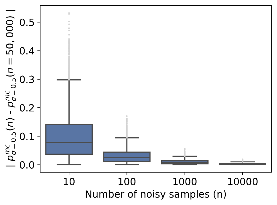
Refer to caption
Refer to caption
Refer to caption
Refer to caption
Refer to caption
Refer to caption
Refer to caption
Refer to caption
Figure 6: Convergence of pσmmsesubscriptsuperscript𝑝mmse𝜎p^{\mathrm{mmse}}_{\sigma}. In practice, pσmmsesubscriptsuperscript𝑝mmse𝜎p^{\mathrm{mmse}}_{\sigma} takes around n=510𝑛510n=5-10 samples to converge and is more computationally inefficient than pσmcsubscriptsuperscript𝑝mc𝜎p^{\mathrm{mc}}_{\sigma}.
Refer to caption
(a) MNIST, Linear
Refer to caption
(b) MNIST, CNN
Refer to caption
(c) FMNIST, Linear
Refer to caption
(d) FMNIST, CNN
Refer to caption
(e) CIFAR10, ResNet18
Refer to caption
(f) CIFAR100, ResNet18
Figure 7: Distribution of pσrobustsubscriptsuperscript𝑝robust𝜎p^{\mathrm{robust}}_{\sigma} over σ𝜎\sigma. As noise increases, pσrobustsubscriptsuperscript𝑝robust𝜎p^{\mathrm{robust}}_{\sigma} decreases. In addition, pσmmsesubscriptsuperscript𝑝mmse𝜎p^{\mathrm{mmse}}_{\sigma} accurately estimates pσmcsubscriptsuperscript𝑝mc𝜎p^{\mathrm{mc}}_{\sigma}.
Refer to caption
(a) MNIST, Linear
Refer to caption
(b) MNIST, CNN
Refer to caption
(c) FMNIST, Linear
Refer to caption
(d) FMNIST, CNN
Refer to caption
(e) CIFAR10, ResNet18
Refer to caption
(f) CIFAR100, ResNet18
Figure 8: Accuracy of pσrobustsubscriptsuperscript𝑝robust𝜎p^{\mathrm{robust}}_{\sigma} estimators over σ𝜎\sigma. The smaller the noise neighborhood σ𝜎\sigma, the more accurately the estimators compute pσrobustsubscriptsuperscript𝑝robust𝜎p^{\mathrm{robust}}_{\sigma}. pσmmsesubscriptsuperscript𝑝mmse𝜎p^{\mathrm{mmse}}_{\sigma} and pσmmse_mvssubscriptsuperscript𝑝mmse_mvs𝜎p^{\mathrm{mmse\_mvs}}_{\sigma} are the best estimators of pσrobustsubscriptsuperscript𝑝robust𝜎p^{\mathrm{robust}}_{\sigma}, followed closely by pσtaylor_mvssubscriptsuperscript𝑝taylor_mvs𝜎p^{\mathrm{taylor\_mvs}}_{\sigma} and pσtaylorsubscriptsuperscript𝑝taylor𝜎p^{\mathrm{taylor}}_{\sigma}, trailed by pTsoftmaxsubscriptsuperscript𝑝softmax𝑇p^{\mathrm{softmax}}_{T}.
Refer to caption
(a) CIFAR10, ResNet18
Refer to caption
(b) CIFAR100, ResNet18
Figure 9: Accuracy of pσrobustsubscriptsuperscript𝑝robust𝜎p^{\mathrm{robust}}_{\sigma} estimators over σ𝜎\sigma for robust models. For more robust models, the estimators compute pσrobustsubscriptsuperscript𝑝robust𝜎p^{\mathrm{robust}}_{\sigma} more accurately over a larger σ𝜎\sigma.
Refer to caption
Figure 10: mv-sigmoid’s approximation of mvn-cdf over σ𝜎\sigma. mv-sigmoid well-approximates mvn-cdf over σ𝜎\sigma.
Refer to caption
(a) MNIST, Linear
Refer to caption
(b) MNIST, CNN
Refer to caption
(c) FMNIST, Linear
Refer to caption
(d) FMNIST, CNN
Refer to caption
(e) CIFAR10, ResNet18
Refer to caption
(f) CIFAR100, ResNet18
Figure 11: Local robustness bias among classes. pσrobustsubscriptsuperscript𝑝robust𝜎p^{\mathrm{robust}}_{\sigma} reveals that the model is less locally robust for some classes than for others. The analytical estimator pσmmsesubscriptsuperscript𝑝mmse𝜎p^{\mathrm{mmse}}_{\sigma} properly captures this model bias.
CPU: Intel x86_64 GPU: Tesla V100-PCIE-32GB
Estimator # samples (n𝑛n) Serial Batched Serial Batched
pσmcsubscriptsuperscript𝑝mc𝜎p^{\mathrm{mc}}_{\sigma}
n=100𝑛100n=100
n=1000𝑛1000n=1000
n=10000𝑛10000n=10000
0:00:59
0:09:50
1:41:11
0:00:42
0:07:22
1:14:38
0:00:12
0:02:00
0:19:56
0:00:01
0:00:04
0:00:35
pσtaylorsubscriptsuperscript𝑝taylor𝜎p^{\mathrm{taylor}}_{\sigma} N/A 0:00:08 0:00:07 0:00:02 << 0:00:01
pσtaylor_mvssubscriptsuperscript𝑝taylor_mvs𝜎p^{\mathrm{taylor\_mvs}}_{\sigma} N/A 0:00:08 0:00:07 0:00:01 << 0:00:01
pσmmsesubscriptsuperscript𝑝mmse𝜎p^{\mathrm{mmse}}_{\sigma}
n=1𝑛1n=1
n=5𝑛5n=5
n=10𝑛10n=10
n=25𝑛25n=25
n=50𝑛50n=50
n=100𝑛100n=100
0:00:08
0:00:41
0:01:21
0:03:21
0:06:47
0:13:57
0:00:10
0:00:31
0:01:02
0:02:44
0:05:38
0:11:31
0:00:02
0:00:06
0:00:11
0:00:26
0:00:51
0:01:42
0:00:02
0:00:02
0:00:02
0:00:03
0:00:04
0:00:06
pσmmse_mvssubscriptsuperscript𝑝mmse_mvs𝜎p^{\mathrm{mmse\_mvs}}_{\sigma}
n=1𝑛1n=1
n=5𝑛5n=5
n=10𝑛10n=10
n=25𝑛25n=25
n=50𝑛50n=50
n=100𝑛100n=100
0:00:08
0:00:41
0:01:21
0:03:24
0:06:47
0:13:28
0:00:08
0:00:32
0:01:00
0:02:37
0:05:35
0:11:32
0:00:01
0:00:05
0:00:10
0:00:25
0:00:51
0:01:42
0:00:01
0:00:01
0:00:02
0:00:02
0:00:03
0:00:06
pTsoftmaxsubscriptsuperscript𝑝softmax𝑇p^{\mathrm{softmax}}_{T} N/A 0:00:01 << 0:00:01 << 0:00:01 << 0:00:01
Table 3: Runtimes of each pσrobustsubscriptsuperscript𝑝robust𝜎p^{\mathrm{robust}}_{\sigma} estimator. Each estimator computes pσ=0.1robustsubscriptsuperscript𝑝robust𝜎0.1p^{\mathrm{robust}}_{\sigma={0.1}} for the CIFAR10 ResNet18 model for 50 data points. For estimators that use sampling, the row with the minimum number of samples necessary for convergence is italicized. Runtimes are in the format of hour:minute:second. The analytical estimators (pσtaylorsubscriptsuperscript𝑝taylor𝜎p^{\mathrm{taylor}}_{\sigma}, pσtaylor_mvssubscriptsuperscript𝑝taylor_mvs𝜎p^{\mathrm{taylor\_mvs}}_{\sigma}, pσmmsesubscriptsuperscript𝑝mmse𝜎p^{\mathrm{mmse}}_{\sigma}, and pσmmse_mvssubscriptsuperscript𝑝mmse_mvs𝜎p^{\mathrm{mmse\_mvs}}_{\sigma}) are more efficient than the naïve estimator (pσmcsubscriptsuperscript𝑝mc𝜎p^{\mathrm{mc}}_{\sigma}).

A.4.1 pσrobustsubscriptsuperscript𝑝robust𝜎p^{\mathrm{robust}}_{\sigma} identifies images that are robust to and images that are vulnerable to random noise

For each dataset, we train a simple CNN to distinguish between images with high and low pσmmsesubscriptsuperscript𝑝mmse𝜎p^{\mathrm{mmse}}_{\sigma}. We train the same CNN to also distinguish between images with high and low pTsoftmaxsubscriptsuperscript𝑝softmax𝑇p^{\mathrm{softmax}}_{T}. The CNN consists of two convolutional layers and two fully-connected feedforward layers with a total of 21,878 parameters. For a given dataset, for each class, we take the images with the top-25 and bottom-25 pσmmsesubscriptsuperscript𝑝mmse𝜎p^{\mathrm{mmse}}_{\sigma} values. This yields 500 images for CIFAR10 (10 classes x 50 images per class) and 5,000 images for CIFAR100 (100 classes x 50 images per class). We also perform the same steps using pTsoftmaxsubscriptsuperscript𝑝softmax𝑇p^{\mathrm{softmax}}_{T}, yielding another 500 images for CIFAR10 and another 5,000 images for CIFAR100. For each dataset, the train/test split is 90%/10% of points.

Then, we compare the performance of the two models. For CIFAR10, the test set accuracy for the pσmmsesubscriptsuperscript𝑝mmse𝜎p^{\mathrm{mmse}}_{\sigma} CNN is 0.92 while that for the pTsoftmaxsubscriptsuperscript𝑝softmax𝑇p^{\mathrm{softmax}}_{T} CNN is 0.58. For CIFAR100, the test set accuracy for the pσmmsesubscriptsuperscript𝑝mmse𝜎p^{\mathrm{mmse}}_{\sigma} CNN is 0.74 while that for the pTsoftmaxsubscriptsuperscript𝑝softmax𝑇p^{\mathrm{softmax}}_{T} CNN is 0.55. The higher the test set accuracy of a CNN, the better the CNN distinguishes between images. Thus, the results indicate that pσrobustsubscriptsuperscript𝑝robust𝜎p^{\mathrm{robust}}_{\sigma} better identifies images that are robust to and vulnerable to random noise than pTsoftmaxsubscriptsuperscript𝑝softmax𝑇p^{\mathrm{softmax}}_{T}.

We also provide additional visualizations of images with the highest and lowest pσrobustsubscriptsuperscript𝑝robust𝜎p^{\mathrm{robust}}_{\sigma} and images with the highest and lowest pTsoftmaxsubscriptsuperscript𝑝softmax𝑇p^{\mathrm{softmax}}_{T}.

Car                           Boat

Lowest pσ=0.1mmsesubscriptsuperscript𝑝mmse𝜎0.1p^{\mathrm{mmse}}_{\sigma={0.1}}                Highest pσ=0.1mmsesubscriptsuperscript𝑝mmse𝜎0.1p^{\mathrm{mmse}}_{\sigma={0.1}}               Lowest pTsoftmaxsubscriptsuperscript𝑝softmax𝑇p^{\mathrm{softmax}}_{T}               Highest pTsoftmaxsubscriptsuperscript𝑝softmax𝑇p^{\mathrm{softmax}}_{T}

Refer to caption
Refer to caption
Refer to caption
Refer to caption
Refer to caption
Refer to caption
Refer to caption
Refer to caption
Figure 12: Additional images with the lowest and highest pσrobustsubscriptsuperscript𝑝robust𝜎p^{\mathrm{robust}}_{\sigma} and pTsoftmaxsubscriptsuperscript𝑝softmax𝑇p^{\mathrm{softmax}}_{T} values among CIFAR10 classes. Images with high pσrobustsubscriptsuperscript𝑝robust𝜎p^{\mathrm{robust}}_{\sigma} tend to be brighter and have stronger object-background contrast (making them more robust to random noise) than those with low pσrobustsubscriptsuperscript𝑝robust𝜎p^{\mathrm{robust}}_{\sigma}. The difference between images with high and low pTsoftmaxsubscriptsuperscript𝑝softmax𝑇p^{\mathrm{softmax}}_{T} is less clear. Thus, pσrobustsubscriptsuperscript𝑝robust𝜎p^{\mathrm{robust}}_{\sigma} better captures the model’s local robustness with respect to an input than pTsoftmaxsubscriptsuperscript𝑝softmax𝑇p^{\mathrm{softmax}}_{T}.

Cloud                         Bicycle

Lowest pσ=0.05mmsesubscriptsuperscript𝑝mmse𝜎0.05p^{\mathrm{mmse}}_{\sigma={0.05}}               Highest pσ=0.05mmsesubscriptsuperscript𝑝mmse𝜎0.05p^{\mathrm{mmse}}_{\sigma={0.05}}               Lowest pTsoftmaxsubscriptsuperscript𝑝softmax𝑇p^{\mathrm{softmax}}_{T}               Highest pTsoftmaxsubscriptsuperscript𝑝softmax𝑇p^{\mathrm{softmax}}_{T}

Refer to caption
Refer to caption
Refer to caption
Refer to caption
Refer to caption
Refer to caption
Refer to caption
Refer to caption
Figure 13: Images with the lowest and highest pσrobustsubscriptsuperscript𝑝robust𝜎p^{\mathrm{robust}}_{\sigma} and pTsoftmaxsubscriptsuperscript𝑝softmax𝑇p^{\mathrm{softmax}}_{T} values among CIFAR100 classes. Images with high pσrobustsubscriptsuperscript𝑝robust𝜎p^{\mathrm{robust}}_{\sigma} tend to be brighter and have stronger object-background contrast (making them more robust to random noise) than those with low pσrobustsubscriptsuperscript𝑝robust𝜎p^{\mathrm{robust}}_{\sigma}. The difference between images with high and low pTsoftmaxsubscriptsuperscript𝑝softmax𝑇p^{\mathrm{softmax}}_{T} is less clear. Thus, pσrobustsubscriptsuperscript𝑝robust𝜎p^{\mathrm{robust}}_{\sigma} better captures the model’s local robustness with respect to an input than pTsoftmaxsubscriptsuperscript𝑝softmax𝑇p^{\mathrm{softmax}}_{T}.

Digit 2               Digit 1              Digit 0

Original            σ=0.2𝜎0.2\sigma=0.2             σ=0.4𝜎0.4\sigma=0.4             σ=0.6𝜎0.6\sigma=0.6             σ=0.8𝜎0.8\sigma=0.8             σ=1.0𝜎1.0\sigma=1.0

Refer to caption
Refer to caption
Refer to caption
Figure 14: Examples of noisy images for MNIST.

Ankle boot           Trousers               Shirt

Original            σ=0.2𝜎0.2\sigma=0.2             σ=0.4𝜎0.4\sigma=0.4             σ=0.6𝜎0.6\sigma=0.6             σ=0.8𝜎0.8\sigma=0.8             σ=1.0𝜎1.0\sigma=1.0

Refer to caption
Refer to caption
Refer to caption
Figure 15: Examples of noisy images for FMNIST.

Ship                Airplane               Deer

Original           σ=0.02𝜎0.02\sigma=0.02           σ=0.04𝜎0.04\sigma=0.04           σ=0.06𝜎0.06\sigma=0.06           σ=0.08𝜎0.08\sigma=0.08            σ=0.1𝜎0.1\sigma=0.1

Refer to caption
Refer to caption
Refer to caption
Figure 16: Examples of noisy images for CIFAR10.

Lion                 Cloud                 Sea

Original           σ=0.02𝜎0.02\sigma=0.02           σ=0.04𝜎0.04\sigma=0.04           σ=0.06𝜎0.06\sigma=0.06           σ=0.08𝜎0.08\sigma=0.08            σ=0.1𝜎0.1\sigma=0.1

Refer to caption
Refer to caption
Refer to caption
Figure 17: Examples of noisy images for CIFAR100.