Learning to Design Analog Circuits to Meet Threshold Specifications

Abstract

Automated design of analog and radio-frequency circuits using supervised or reinforcement learning from simulation data has recently been studied as an alternative to manual expert design. It is straightforward for a design agent to learn an inverse function from desired performance metrics to circuit parameters. However, it is more common for a user to have threshold performance criteria rather than an exact target vector of feasible performance measures. In this work, we propose a method for generating from simulation data a dataset on which a system can be trained via supervised learning to design circuits to meet threshold specifications. We moreover perform the to-date most extensive evaluation of automated analog circuit design, including experimenting in a significantly more diverse set of circuits than in prior work, covering linear, nonlinear, and autonomous circuit configurations, and show that our method consistently reaches success rate better than 90% at 5% error margin, while also improving data efficiency by upward of an order of magnitude. A demo of this system is available at circuits.streamlit.app

1 Introduction

Owing to the immense growth of consumer electronics over the last few decades, integrated circuitry using commercial CMOS/BiCMOS chip technologies has become a major sector of the semiconductor industry (Kamal, 2022). More specifically, fast innovation and skyrocketing demand in several industry segments, such as wireless communication and high-resolution imaging systems, has been driving interest in analog, radio-frequency, and millimeter-wave circuits and systems (Kamal, 2022). Despite the economic and technological importance of these types of circuits, contemporary design in research and industry is still predominantly manual, using advanced electronic design automation tools such as the Cadence Virtuoso (Martin, 2002) and the Keysight ADS (Kouhalvandi et al., 2018) circuit simulators. This heavy reliance on human design slows down and raises the costs of the development of future generations of electronic systems and should inevitably shift toward a more interactive design approach where humans and machines co-design analog circuits substantially faster.

A recent growing literature on automated circuit design has considered the problem of finding the parameters of components in a given circuit that would induce a desired set of performance metrics (Mina et al., 2022). Learning to output such circuit parameters is typically framed in the supervised learning setting, where a model in a given model class — often a neural network — is trained on a dataset of simulated parameter–metrics pairs to solve the inverse problem of mapping target performance metrics to circuit parameters that meet these requirements. A limiting factor in this approach is the large number of times that the circuit needs to be simulated to collect enough data for accurate learning. As we aim to support larger and more intricate circuits, precise simulation becomes slow, and data efficiency requisite.

We address two inverse problems. For the simpler one, described above and formalized in Section 2.1, a dataset is created by simulating a circuit with parameter values on a grid that covers a user-specified range. A neural network is then trained on this data to predict circuit parameters that would induce a desired performance vector. We evaluate this approach on a much larger variety of useful circuit topologies than has previously been done, and show that this inverse function is smooth and regular enough to be approximated from a much smaller number of examples than achieved before, namely around 600–4000 points, depending on circuit complexity, compared with 10,000 to 40,000 points in prior work (Fukuda et al., 2017b; Wang et al., 2018b; Lourenço et al., 2018; M.V. & Harish, 2020b).

However, this approach has severely limited usability, because it requires the user to make a rather precise guess of a feasible combination of performance metrics for the model to recover. As the number of metrics of interest grows, in more complex circuits, the task of precisely specifying all metrics becomes daunting. We instead envision an interface for a user to specify a vector of performance thresholds, and propose a second inverse problem of mapping these thresholds into circuit parameters that satisfy them (Section 2.2). While this problem is natural for reinforcement learning algorithms (Settaluri et al., 2020), we propose a novel supervised learning method for constructing, from the same simulation data as in the simpler problem, a dataset for training and evaluating a model that predicts threshold-satisfying parameters. We show that training a neural network on this dataset solves this harder inverse problem an order of magnitude more efficiently than existing reinforcement learning methods, the latter using between 5500 and 40,000 simulations (Wang et al., 2018a; Settaluri et al., 2020).

This work contributes: (1) a novel and vastly more data-efficient method for generating, from circuit simulation data, a dataset for supervised learning of circuit design agents for the threshold specification problem; and (2) the to-date most extensive evaluation of automated circuit design methods on a diverse set of analog and radio frequency circuits, demonstrating the success of the method while also identifying a challenging circuit topology for future research. A demo of our proposed system is available at circuits.streamlit.app.

2 Problem Statement

Human design through the use of advanced electronic design automation (EDA) tools (Afacan et al., 2021) is currently the primary method for designing electronic circuits. However, human-led design is a slow process and is falling behind the human–computer co-design processes for digital circuits (Renner & Ekárt, 2003). In order to bridge the gap and allow for faster design of analog circuits, we aim to facilitate a system that can automatically generate the parameters of an analog circuit to meet a set of performance requirements. A good system should be able to function with good accuracy across a variety of different circuit topologies. In this paper, we therefore examine the problem of designing a diverse group of analog circuits, including single-stage amplifiers, multi-stage operational amplifiers, power amplifiers, low-noise amplifiers, nonlinear circuits such as mixers, and autonomous circuits such as voltage-controlled oscillators. It is noteworthy that the selected performance metrics, themselves diverse across the various circuits, exhibit different kinds of correlations and tradeoffs.

2.1 Exact Specification

For a specified circuit topology, let $n$ be the number of component parameters, such as resistances, transistor widths, and voltages. Let $X_{1},\ldots,X_{n}$ be the operational ranges of each of these parameters, and $X=\bigtimes_{i=1}^{n}X_{i}$ the design space. We assume the availability of a simulator $f:X\to Y$, where $Y=\mathbb{R}_{+}^{k}$ is the positive orthant of the real vector space of $k$ performance metrics of interest.

The problem of design from exact specification is that of finding a function $g\approx f^{-1}:Y\to X$ such that, when a user specifies target performance $y\in Y$, the system can suggest a design $\hat{x}=g(y)$. Upon suggesting $\hat{x}$, it can be simulated to measure its performance $\hat{y}=f(\hat{x})$. The error of the system is measured by the relative difference in its performance metrics

$$\delta_{i}=\frac{|y_{i}-\hat{y}_{i}|}{y_{i}}.$$ (1)

For evaluation, the relative error is averaged across multiple test points as well as across the $k$ metrics. We also measure the success rate as the fraction of test points with relative error within a given margin.

We note that, in a real-world system, users can input a target performance vector $y$ for which no circuit exists with low error. The system can use the simulator to check that the predicted circuit $g(y)$ is incorrect, but it is a hard problem to determine whether another circuit would be correct, particularly if the instance is out-of-distribution for the data used to train the system. We therefore focus on evaluating the system on in-distribution data $y\in f(X)$, and leave the challenging and interesting question of out-of-distribution generalization to future work.

2.2 Threshold Specification

When manual circuit design is challenging, guessing a feasible performance vector $y\in f(X)$ can be just as challenging, particularly if it consists of many metrics that are subject to intricate tradeoffs. Instead, it would be easier for a user to specify performance thresholds that the designed circuit should meet. We denote by $\lambda_{i}$ the threshold direction of metric $i$, i.e. $\lambda_{i}=1$ or $-1$ respectively whether it is majorative (the more the better) or minorative (the less the better).

Figure 1: The problem of automated design by threshold specification. A user specifies threshold constraints on the circuit’s performance metrics. A design agent then generates a circuit that, when simulated, meets the constraints.

The problem of design from threshold specification (Figure 1) is that of finding a function $g:Y\to X$ such that, when a user specifies target performance thresholds $y\in Y$, the suggested design $\hat{x}=g(y)$ aims to meet the thresholds $y$ by having its simulated performance $\hat{y}=f(\hat{x})$ satisfy $\lambda\hat{y}\geq\lambda y$ element-wise. The error of this system is measured by the relative amount of threshold violation

$$\delta_{i}=\frac{\max\{\lambda_{i}(y_{i}-\hat{y}_{i}),0\}}{y_{i}}.$$ (2)

As before, we measure success rate by the fraction of test data for which the thresholds for all metrics are met up to a given error margin.

To evaluate a system solving the threshold specification problem, we should use threshold queries that follow a similar distribution to that of real users. Leaving user studies to future work, we approximate this distribution by perturbing simulated performance metrics similarly to Lourenço et al. (2018). Given the measured performance $y=f(x)$ of a simulated circuit $x$, we sample standard uniform perturbations $u\sim\mathrm{U}^{k}$ for the $k$ metrics, independent and identically distributed (i.i.d), and use the perturbed vector

$$\tilde{y}_{i}=(1-\epsilon\lambda_{i}u_{i})y_{i}$$ (3)

as the threshold query. Here $\epsilon$ is the perturbation magnitude hyperparameter; in this work we use $\epsilon=0.2$. Note that, by construction, $\lambda y\geq\lambda\tilde{y}$, so that there always exists a circuit (namely, $x$) that meets the threshold $\tilde{y}$.

3 Related Work

3.1 Digital Circuits vs. Analog Circuits

Digital circuit automation and computer-assisted design (CAD) has progressed steadily over the past few decades (Micheli, 1994; Brunvand, 2010). The invariant architecture of the building blocks in digital design allows the application of graph-theoretic approaches that treat the problem of digital circuit design as a graph connectivity problem, which has led to a large body of work in optimization of digital design (Boyd et al., 2005; Kunz & Pradhan, 1994; Grover & Chaudhary, 2014). Analog circuits, on the other hand, involve a set of unique design challenges that are not considered in the digital domain. First, analog circuits have a broad range of architectures, and each building block may be optimized individually with respect to a performance metric before all the blocks are integrated into the circuit. Second, in digital design, there is a small set of critical performance metrics and in most cases only power consumption, area, and speed are considered. In contrast, in the analog domain, a variety of performance metrics are present, and optimization of an analog circuit becomes a higher-dimensional problem. Third, in analog circuits, passive components such as capacitors, inductors, and resistors are also deployed, completely changing the dynamics of the circuit design and weakening the relation between graph-theoretic properties and circuit performance.

3.2 Automated Analog Circuit Design

Automating the design of analog circuits has been studied before, particularly in operational amplifiers (op-amps) that are specified by their voltage gain, bandwidth, and power consumption (for a survey, see Mina et al. (2022)). Wang et al. (2018a) propose a reinforcement learning (RL) approach to designing 3-stage amplifier circuits from threshold specification. Similarly, Settaluri et al. (2020) adopt RL to design 2-stage operational amplifiers. While RL is readily amenable to threshold constraints, it suffers from poor data efficiency compared with supervised learning approaches (Mina et al., 2022). Vural et al. (2015) use supervised regression to design another type of circuits, a 4-bit current-steering Digital-to-Analog converters (DAC), from exact specification of the performance metrics. Other works have used supervised learning to design various op-amps (Harsha & Harish, 2020; Lourenço et al., 2018; Murphy & McCarthy, 2021) with varying — and often incomparable — data efficiency (Mina et al., 2022).

In this paper, we step beyond the scope of op-amp design to additionally investigate the design of other critical analog circuit blocks, in particular radio-frequency electronic circuits that are commonly used in cellular communication applications (Razavi, 2012). It is noteworthy that some of the selected circuits, e.g., mixers and oscillators, are among the most nonlinear analog circuits with high sensitivity to variations in design parameters. We further show that design agents for amplifiers as well as more intricate circuits can be learned by supervised regression from much smaller datasets than previously accomplished. Finally, we learn to design these circuits from threshold specification, in contrast to most previous supervised learning works. Lourenço et al. (2018) previously considered this setting, and proposed a method that we reproduce in this paper under the name $D^{m}_{\epsilon}$. We show that this method can lead to suboptimal performance, analyze the reason through an ablation study, and propose a new method that mitigates this issue.

4 Method

Figure 2: Proposed method for automated design from threshold specification. Circuit parameters are sampled within a user-defined range, simulated, and measured. Performance metrics are randomly adjusted to sample threshold queries. A data filtering process then generates training data for supervised learning a circuit design agent that generates circuits to meet threshold requirements.

We use supervised learning to approximate the inverse of the simulator function mapping circuit parameters to performance metrics (Figure 2). We interface an external simulator to generate a dataset $D_{0}$ consisting of circuit parameter vectors $x\in\mathbb{R}^{n}$ and their respective measured performance metrics vectors $y\in\mathbb{R}^{k}$. We (optionally) pass this dataset through a filtering pipeline that prepares it for solving the threshold specification problem (Section 2.2). Finally, we employ a supervised learning algorithm, such as gradient-based optimization, to train a design agent. In this section we describe the system components: the simulator, the agent model, and several alternatives for the filtering pipeline.

4.1 Simulator

In this work, we use the NgSpice simulator (Nenzi & Vogt, 2011). The circuit topology and its fixed parameters, as well as the simulation parameters, are provided to the simulator via a format called netlist (Lannutti et al., 2012). In addition to the netlist, the simulator loads analysis commands that determine how it measures the performance metrics of interest. For some circuits, multiple analysis commands are given to measure the circuit under distinct conditions.

The external simulator is wrapped by a Python interface to allow easy access to two functionalities. First, to generate simulation data, a user inputs the range and step size of each circuit parameter, and the simulator loops through this grid to output a dataset $D_{0}$ of parameter–metrics pairs. Second, to evaluate the trained model, predicted circuit parameters are input to the simulator, and the measured performance is compared with the target performance.

4.2 Agent Model

Before the raw data from the simulator can be put through the model, we apply a few data pre-processing steps. The different features of the data have vastly different scales. In order to allow the model to learn across such different scales, we first shift and scale all values to the range $[-1,1]$. This normalization is applied both to the performance metrics before they are fed to the model and to the ground-truth circuit parameters used for training, and an appropriate inverse operator is applied to the model’s parameter predictions.

In this work, we experiment with three different agent models. The main model is a neural network with an architecture of a simple multi-layer perceptron, trained with the Adam optimizer (Kingma & Ba, 2015). The network takes in a vector of desired performance metrics and predicts a vector of circuit parameters, which is then compared with the ground-truth parameters using an absolute ($L_{1}$) loss. The sizes of the first and last layers of the network are adjusted to reflect the number of performance metrics and circuit parameters, respectively, which are different for each experiment described in Section 5. The architecture is otherwise constant across experiments and detailed in Appendix A.1. An alternative model we consider is ensembles of decision trees trained with the Random Forests algorithm (Breiman, 2001). Finally, to assess the need for any learning at all, we compare with a lookup method that memorizes the training data and selects, for each test performance vector, the training circuit that minimizes the relative performance error.

4.3 Filtering Pipeline

The problem of design from exact specification (Section 2.1) can be solved by supervised learning, in which the training set is the simulation dataset $D_{0}$, inverted so that performance metrics $y$ are inputs and circuit parameters $x$ are outputs. However, this method is unlikely to be sufficient for the threshold specification problem (Section 2.2), in which some threshold vectors are out-of-distribution for $D_{0}$, because no circuit has them as its exact performance. We therefore propose a filtering pipeline that constructs, from the same $D_{0}$, a second dataset which, when used for supervised learning, trains a model that predicts circuit parameters from threshold specification.

To prepare a circuit for the threshold specification problem, two properties of the metrics vector need to be provided. First, because some metrics, such as gain or bandwidth, are majorative (the more the better), while others, such as power consumption, are minorative (the less the better), we need to know for each metric $i$ its threshold direction $\lambda_{i}\in\{-1,1\}$. Second, a specification asking for the highest gain at power consumption at most $p$ is different from one asking for the lowest power consumption that achieves gain at least $g$. We may therefore have a preference order over metrics, such that we lexicographically prefer improving $y_{i}$ over improving $y_{j}$, whenever $i<j$, as long as all threshold constraints are approximately met. We say that $y$ is lexicographically better than $y^{\prime}$ if there exists $i$ such that $y_{j}=y^{\prime}_{j}$ for all $j<i$ and $\lambda_{i}y_{i}>\lambda_{i}y^{\prime}_{i}$.

The filtering pipeline starts by finding, for each performance vector $y\in D_{0}$, all feasible performance vectors $y^{\prime}\in D_{0}$ that meet the threshold specification $y$, i.e.

$$F(y;D_{0})=\{(x,y^{\prime})\in D_{0}|\lambda y^{\prime}\geq\lambda y\}.$$ (4)

The design agent needs to map the threshold specification $y$ to one such $x\in F(y)$, but it may not be immediately clear which one. We hypothesize that, crucially to learning with high success rate from small datasets, our training dataset must be systematic in selecting a representative of $F(y)$. This systematicity manifests as a pattern that the learning algorithm can generalize, whereas including the entire $F(y)$ or selecting from it sporadically might lead to conflicts that impede generalization.

We propose to select the lexicographically best training-set circuit that meets the threshold

$$\bar{D}^{*}_{0}=\{(x,y)|y\in D_{0},x=\operatorname*{argmax}F(y;D_{0})\},$$ (5)

where we select for $x$ a single representative $(x,y^{\prime})$ of $F(y)$ that maximizes $y^{\prime}$ lexicographically. In the notation $\bar{D}^{*}_{0}$, the bar denotes feasibility of $x$ for $y$ and the star denotes selection of the best representative.

We note that, by definition, all members of $F(y)$ have good circuit parameters that meet the threshold $y$. However, adding all of them to our training set, similar to the method proposed by Lourenço et al. (2018), would create conflicts where the same network input $y$ is mapped to different outputs. By breaking “ties” in a consistent way — and in accordance with user-specified preference over metrics — we create a dataset more conducive of learning. The new dataset $\bar{D}^{*}_{0}$ has the same size as the simulation dataset $D_{0}$ and the same set of performance vectors. The circuit parameter vectors in $\bar{D}^{*}_{0}$ are those that define its Pareto frontier, that is, for which no other simulated circuit is better in all performance metrics. Thus, $\bar{D}^{*}_{0}$ consistently maps feasible performance vectors to frontier circuits.

4.3.1 Threshold Queries

In Section 2.2, we discussed how performance metrics measured in simulation are perturbed to generate threshold queries (Eq. (3)). We denote thus perturbed data by

$$D_{\epsilon}=\{(x,(1-\epsilon\lambda u)y)|(x,y)\in D_{0},u\sim U^{k}\text{ i.i.d}\}.$$ (6)

Note that the distribution of threshold queries $y\sim D_{\epsilon}$ is different than the distribution of simulated metrics vectors $y\sim\bar{D}^{*}_{0}$. To avoid a mismatch of the training and test distributions, we combine the filters to form a dataset of threshold queries with a principled selection of target circuits:

$$\bar{D}^{*}_{\epsilon}=\{(x,\tilde{y})|\tilde{y}\in D_{\epsilon},x=\operatorname*{argmax}F(\tilde{y};D_{0})\}.$$ (7)

$\bar{D}^{*}_{\epsilon}$ is a dataset mapping $\epsilon$-perturbed metrics vectors $\tilde{y}$ to circuits whose (unperturbed) simulated metrics are feasible for the threshold query $\tilde{y}$, selecting the lexicographically best such circuit.

4.3.2 Baseline and Ablation

We compare our dataset construction methods, $\bar{D}^{*}_{0}$ and $\bar{D}^{*}_{\epsilon}$, with a baseline that closely follows Lourenço et al. (2018). We define $D^{m}_{\epsilon}$ as the union of $m$ i.i.d. samples of $D_{\epsilon}$

$$D^{m}_{\epsilon}=\bigcup_{t=1}^{m}D_{\epsilon}[u_{t}];\quad u_{t}\sim U^{k}\text{ i.i.d}.$$ (8)

In our experiments, $m=20$. The reasons are that by construction, in each $(x,\tilde{y})\in D^{m}_{\epsilon}$ the circuit $x$ is feasible for the threshold query $\tilde{y}$, i.e. $\lambda f(x)\geq\lambda\tilde{y}$ ; and that the training distribution $\tilde{y}\sim D^{m}_{\epsilon}$ is identical to our evaluation distribution $\tilde{y}\sim D_{\epsilon}$. Note that, in contrast to most of the literature on analog circuit design automation via supervised learning, which employs a simulation dataset akin to $D_{0}$, $D^{m}_{\epsilon}$ is suited for the threshold specification problem (Lourenço et al., 2018).

Unfortunately, the dataset $D^{m}_{\epsilon}$ can be very confusing to learn from. Because the simulator function $f$ is not necessarily injective, there may exist multiple circuits with similar performance vectors. Moreover, such vectors have overlapping supports of their perturbation distributions. The result is that $D^{m}_{\epsilon}$ will tend to have similar threshold queries mapped to vastly different circuit parameters, rendering their prediction difficult.

We propose an ablation that more directly demonstrates this issue. In $\bar{D}^{m}_{\epsilon}$, we select for each $\tilde{y}\in D_{\epsilon}$ the $m$ lexicographically-best feasible circuits, rather than only the single best in $\bar{D}^{*}_{\epsilon}$ (Eq. (7)):

$$\bar{D}^{m}_{\epsilon}=\{(x,\tilde{y})|\tilde{y}\in D_{\epsilon},x\in\operatorname*{top\mathnormal{-m}}F(\tilde{y};D_{0})\}.$$ (9)

We expect this method to perform suboptimally, more similarly to $D^{m}_{\epsilon}$ than to $\bar{D}^{*}_{\epsilon}$. This would provide evidence that the main aspect impacting the prior method, compared with the novel one, is the existence of multiple targets for each query, rather than the other differences — namely, the selection of circuits from the feasible set $F(y)$, or the preference of lexicographically better circuits.

To summarize, we consider six datasets: (1) $D_{0}$ is the simulation data; (2) $D_{\epsilon}$ has perturbed performance metrics that resemble the threshold query distribution, and is used for method evaluation; (3) $\bar{D}^{*}_{0}$ and (4) $\bar{D}^{*}_{\epsilon}$ are our proposed methods, without and with perturbation to match the test distribution; (5) $D^{m}_{\epsilon}$ is a baseline similar to Lourenço et al. (2018); and (6) $\bar{D}^{m}_{\epsilon}$ is an ablation study.

5 Experiments

We experiment with our methods on a diverse group of seven circuit topologies, detailed below. Best practices in circuit design suggest that circuit parameters are chosen based on their impact on performance metrics  (Bandler & Chen, 1988; Hassan et al., 2016; Bandler & Rayas-Sánchez, 2023). Only these parameters are used to optimize performance for each circuit. We simulate each circuit in a parameter grid consisting of approximately 4000 points, except for the simplest two-stage amplifier with around 600 points, as presented in Table 6 in Appendix A.5. A schematic of each circuit shows the range and step size of each variable parameter, as well as color-coded tags illustrating the diversity of the circuits to which our method applies. To facilitate result reproduction, the code and data used in our experiments are available at github. The supplementary details of the circuits employed in our experiments can be found in Tables 8, 9, and 10 in Appendix A.5.

Our main method uses the $\bar{D}^{*}_{\epsilon}$ dataset to train a neural network and evaluate its success rate in 10-fold cross-validation. For each circuit topology, we perform three comparisons of this method. First, we compare the main method with the five other data construction methods described in the previous section. Second, we compare the gradient-based learning algorithm with Random Forests and a simple lookup method (Section 4.2). Third, we study the sensitivity to the amount of training data by varying it. We compare the success rate of 10-fold cross validation, which uses 90% of the data for training each fold, with using 5%, 10%, 20% and 50% of the data for training. We do this by randomly splitting the data into (respectively) 20, 10, 5, and 2 disjoint subsets, training on one subset, testing on the rest, and then averaging the result across the splits.

In all plots in this section, the solid curve is the average over 10 runs of data splitting and training, and the shaded area is the standard-error of the mean (SEM) over those runs.

5.1 Analog Voltage Amplifiers

5.1.1 Common Source (CS) Amplifier

Due to its simplicity, the common source (CS) amplifier (Figure 3(a)) is among the most popular amplifier configurations using a CMOS transistor. As design variables, we consider the width of the transistor and the resistance of the load resistor $R_{D}$. The target performance metrics, in decreasing importance are: bandwidth, voltage gain, and power consumption.

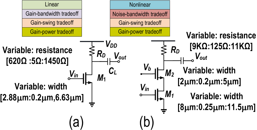
Figure 3: Schematics of analog voltage amplifiers: (a) common source (CS) amplifier; (b) cascode amplifier. Color-coded tags show circuit characteristics. Ranges and step sizes are marked near each circuit parameter.

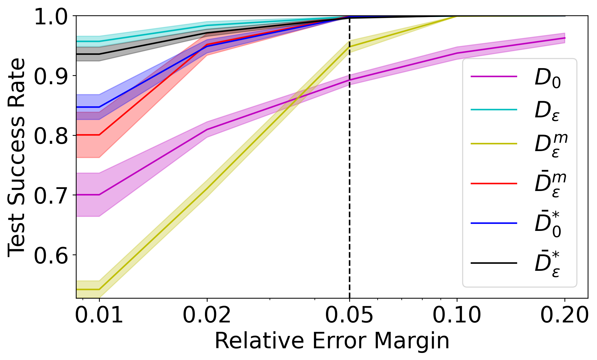
Figure 4: Success rate of designing a CS amplifier: (a) Exact specification: training on $D_{0}$ with varying data sizes and testing on exact metrics $y\sim D_{0}$; (b) Threshold specification: training on varying datasets and testing on threshold metrics $y\sim D_{\epsilon}$.

As shown in Figure 4, our model achieves near-perfect success at 5% error margin on the exact specification problem (Section 2.1), even while using 6 times less data than the best previous work (Devi et al., 2021). In the threshold specification problem (Section 2.2), our model trained on the $\bar{D}^{*}_{\epsilon}$ dataset also achieves perfect success at 5% error margin, whereas training on the naïve $D_{0}$ baseline dataset only achieves 85% success. Note, however, that all other data processing methods also achieve perfect success on this simple circuit. Further results appear in Appendix A.2.

5.1.2 Cascode Amplifier

The CS amplifier has limited gain and exhibits a trade-off between critical performance metrics. The cascode amplifier shown in Figure 3(b) enhances the amplification bandwidth compared with a CS stage (Ko & Lin, 2006).

Figure 5: Success rate of designing a cascode amplifier: (a) Exact specification; (b–d) Threshold specification, comparing: (b) different data sizes of the $\bar{D}^{*}_{\epsilon}$ dataset; (c) different datasets; and (d) different agent models.

As illustrated in Figure 5, this more challenging circuit shows more sensitivity to the amount of training data, both in (a) the exact specification and (b) the threshold specification settings. It is also more difficult for the baseline methods to achieve high success rate, particularly when a low error margin is needed: the simulation dataset $D_{0}$ and the “non-injective” datasets $D^{m}_{\epsilon}$ and $\bar{D}^{m}_{\epsilon}$ all tend to generate circuits with higher than 1%, 2%, and rarely even 5% threshold violation (Figure 5). Finally, Figure 5 demonstrates the typical underperformance of the lookup method, showing that learning is needed; while also demonstrating an uncommon case where Random Forests slightly underperforms the neural network.

5.1.3 Two-Stage Amplifier

The circuits of Figure 3 both suffer from limited gain. Two-stage amplifiers, as shown in Figure 6, are excellent replacements of single-stage amplifiers and in particular allow simultaneously achieving higher gain and voltage swing (Gray & Meyer, 1982).

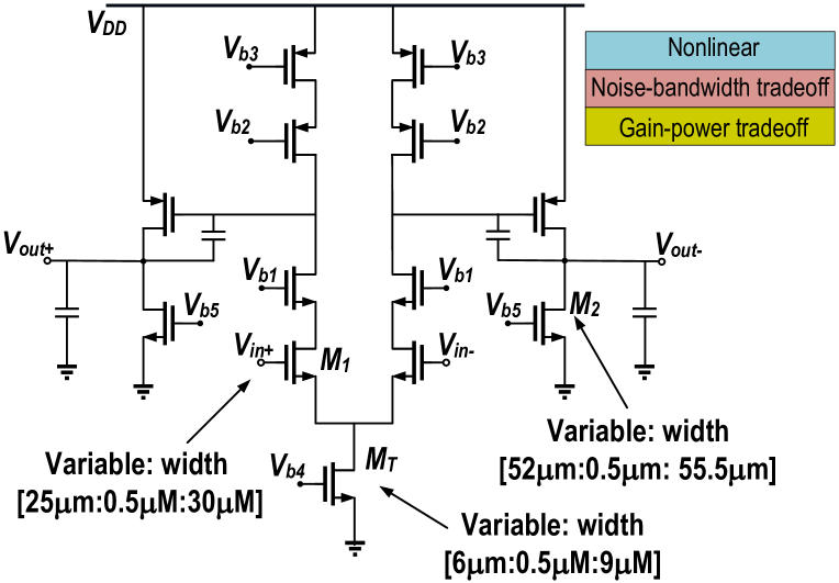
Figure 6: Schematic of a two-stage amplifier.

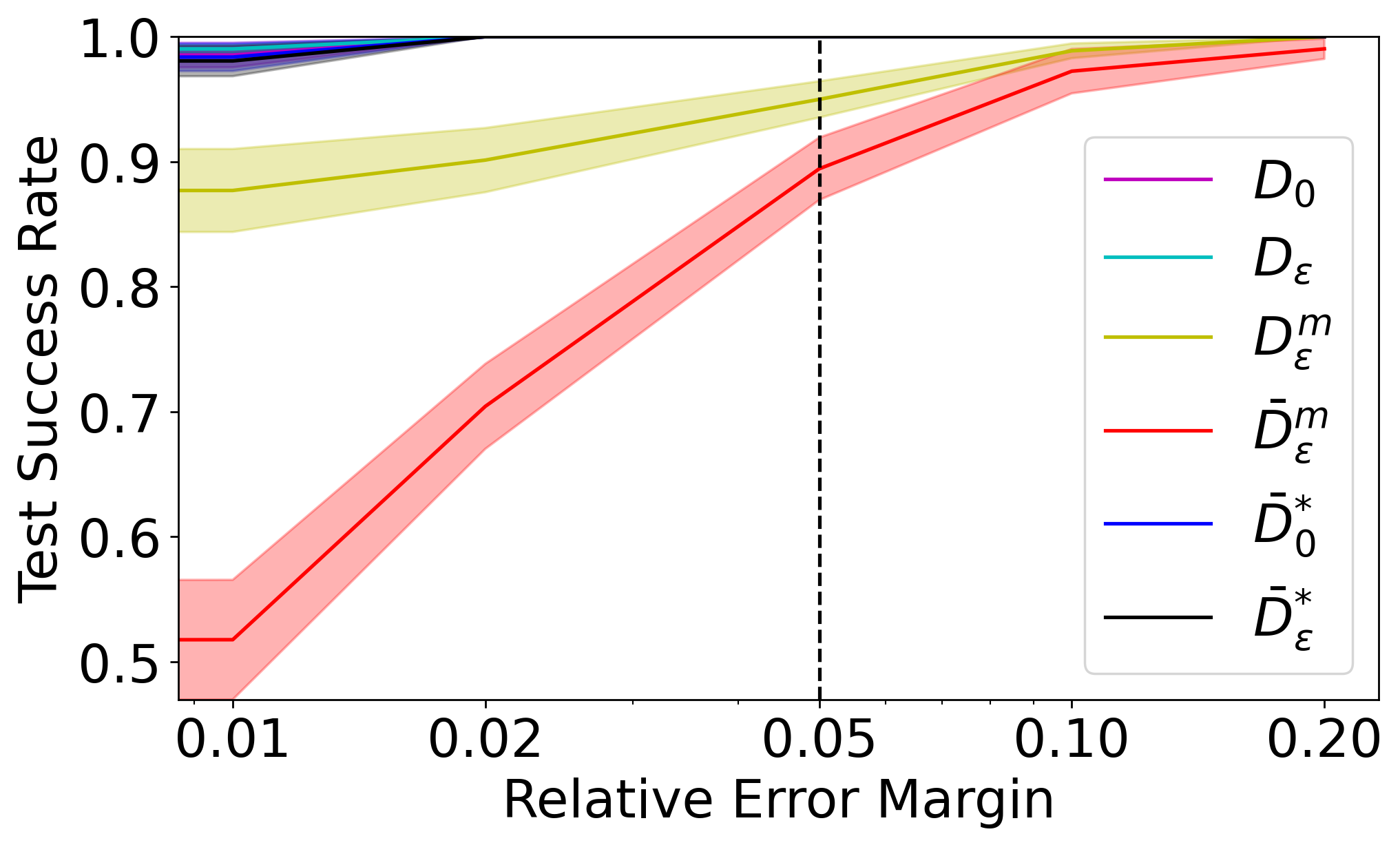
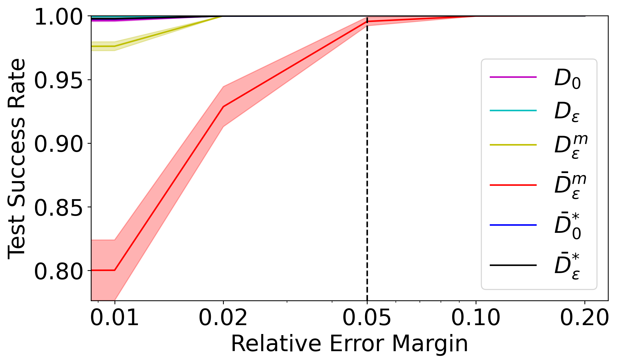
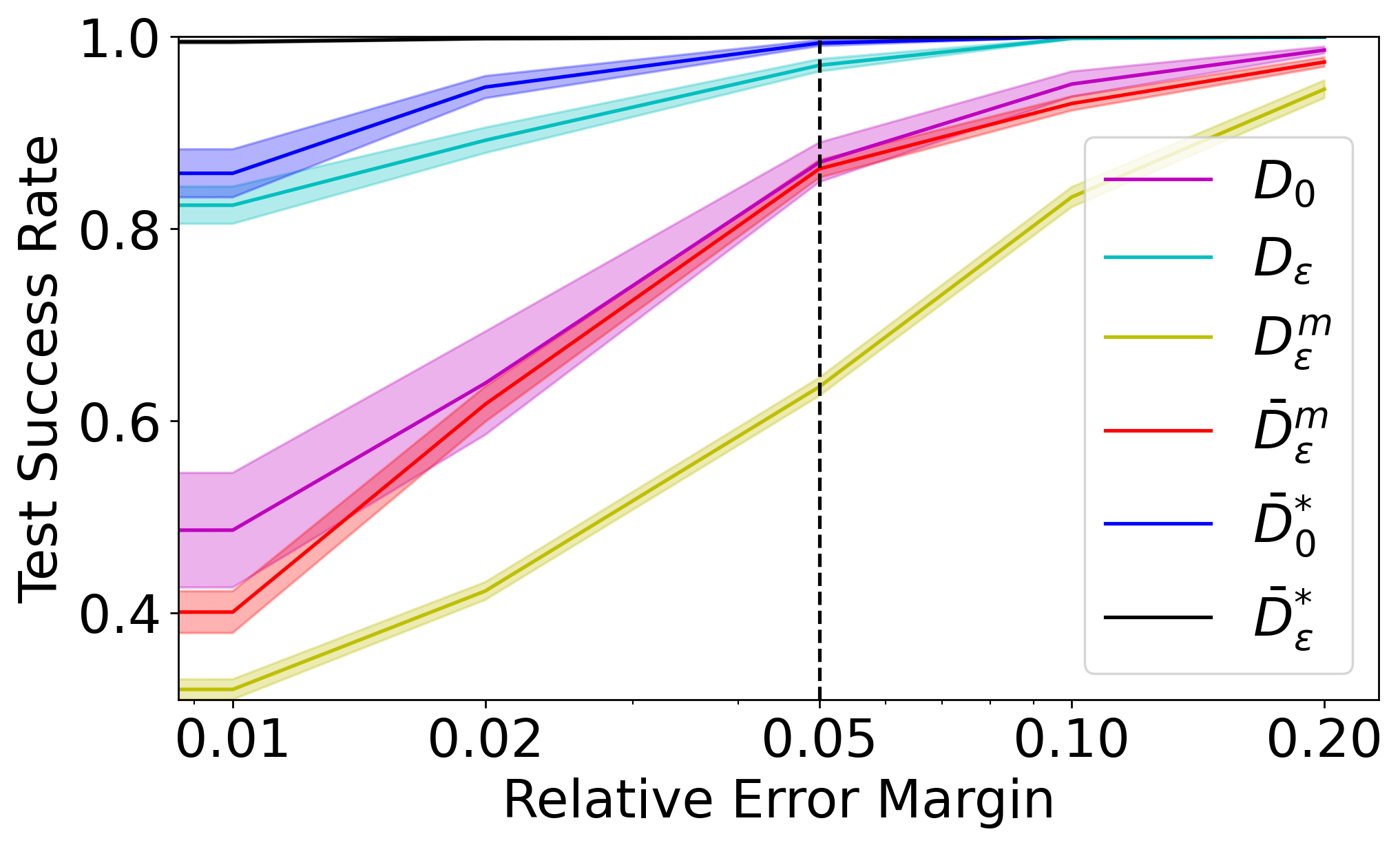
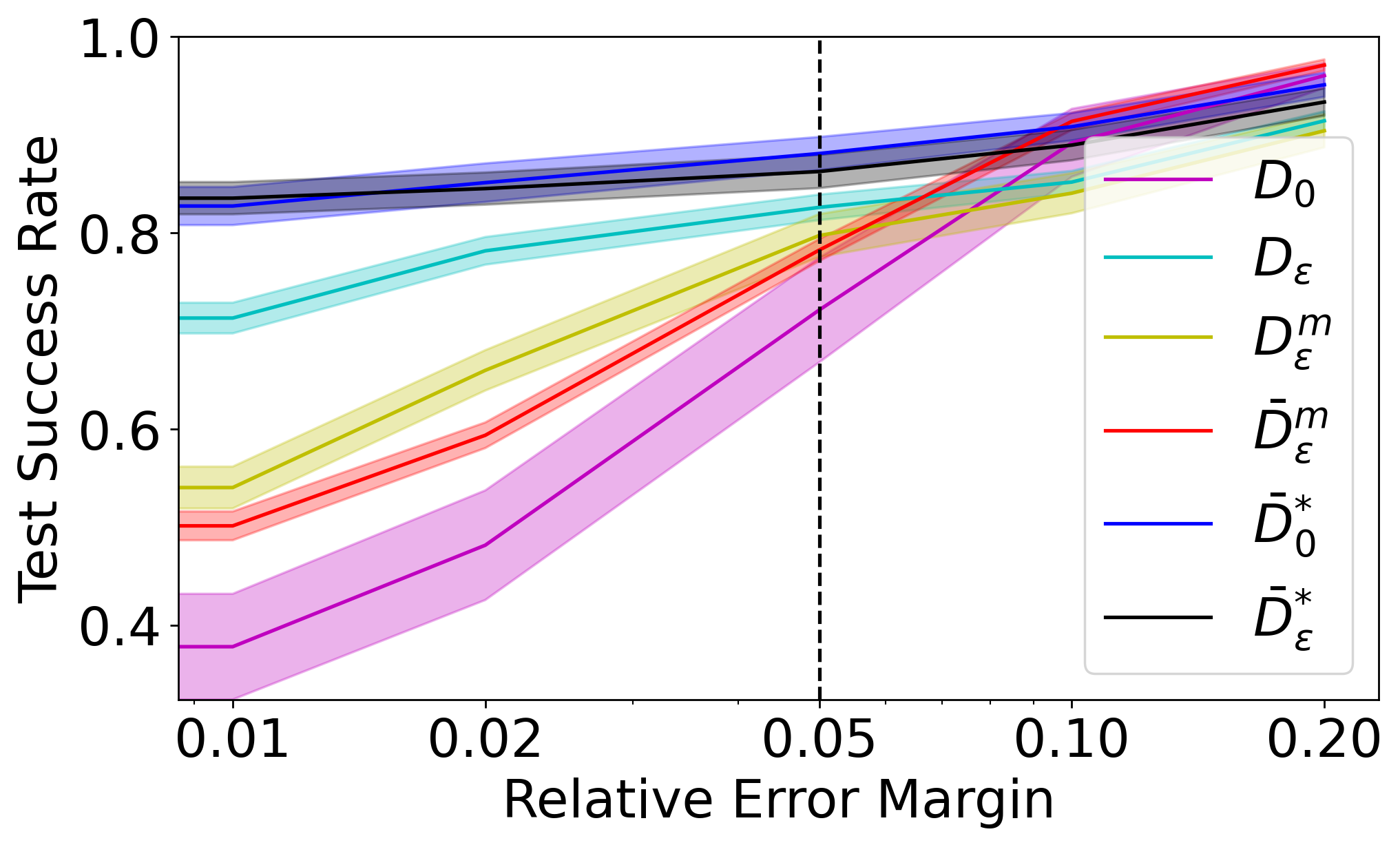
Figure 7: Comparing success rate in the threshold specification problem for different training datasets in five circuits: (a) two-stage; (b) low-noise amplifier (LNA); (c) power amplifier (PA); (d) mixer; (e) voltage-controlled oscillator (VCO).

Owing to their widespread use, two-stage amplifiers have been among the most popular benchmark circuit configurations examined in prior automation work (Mina et al., 2022; Settaluri et al., 2020). Other than the baseline dataset $D^{m}_{\epsilon}$ and ablation dataset $\bar{D}^{m}_{\epsilon}$, all other datasets achieve perfect success on this relatively easy circuit (Figure 7), using 10 times less data than in the best previous work (Fukuda et al., 2017b; Wang et al., 2018b; Lourenço et al., 2018; M.V. & Harish, 2020b). The underperformance of the “non-injective” datasets supports our hypothesis that a systematic selection of representative circuits for similar performance levels is needed to facilitate learning of circuit design agents for threshold specification.

5.2 (Non)-Linear Radio Frequency Circuits

5.2.1 Low-Noise Amplifier (LNA)

The cascode low-noise amplifier (LNA) with inductive degeneration is a popular configuration to design an LNA for an RF receiver (Lerdworatawee & Namgoong, 2005). The circuit, depicted in Figure 8(a), can obtain a high gain and minimal loss of input power across a large bandwidth without suffering from additive noise of circuit components (mainly transistors). This circuit has four parameters (three inductor values and one cascode transistor width) and three metrics: the noise figure (signal-to-noise ratio between the input and output), the return loss, and the power gain.

Our findings indicate that the LNA simulation function has a smooth surface, making it easy to invert for all methods, including the baseline, and resulting in perfect success even at very low error margins (Figure 7). Only the ablation method $\bar{D}^{m}_{\epsilon}$ performs suboptimally, suggesting that it is even more prone to inconsistencies than the baseline $D^{m}_{\epsilon}$.

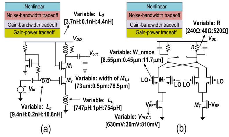
Figure 8: Schematics of: (a) low noise amplifier (LNA); (b) mixer.

5.2.2 Power Amplifier (PA)

A wireless communication transmitter requires a power amplifier to amplify the transmitted signal and deliver more power to the antenna, in order to mitigate the propagation loss of the electromagnetic waves and cover a longer operational distance (Niknejad et al., 2012). An efficient design of a two-stage differential cascode amplifier (Abbasi et al., 2010) that can provide sufficient power gain, while showing efficiency in terms of power consumption, may depend on multiple design parameters (Figure 9(a)).

Similar to LNA, nearly all data filtering methods performed well for the PA circuit, although with higher cross-run variance, with the exception of the baseline $D^{m}_{\epsilon}$ and the ablation $\bar{D}^{m}_{\epsilon}$ (Figure 7). We conclude that both LNA and PA — highly non-linear circuits with intricate tradeoffs, whose design has never before been automated — are easily learned within the operational range tested in this work.

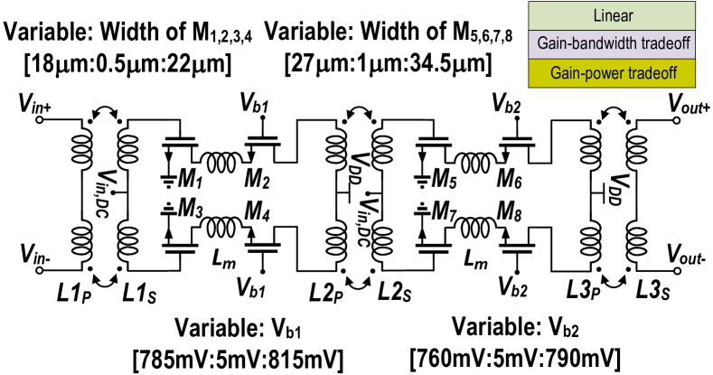
Figure 9: Schematic of a power amplifier (PA).

5.2.3 Mixer

An essential component in frequency conversion of modern radio-frequency and millimeter-wave circuits is a mixer. Given two input signals at frequencies $f_{1}$ and $f_{2}$, a mixer can generate desired signals at subtraction and summation frequencies, i.e., $f_{\Delta}=|f_{1}-f_{2}|$ and $f_{\Sigma}=f_{1}+f_{2}$. Shown in Figure 8(b) is a common schematic for mixers known as a Gilbert Cell (Gilbert, 1968). This circuit operates by having radio frequency (RF) and local oscillation (LO) signals as the inputs and multiplying them to generate a signal with the summation or subtraction frequencies.

The mixer is a sufficiently complex circuit that different data filtering methods achieve different performance when learning to design it (Figure 7). Our proposed method, $\bar{D}^{*}_{\epsilon}$, achieves near-perfect success even at very low error margins, and only our other method, $\bar{D}^{*}_{0}$, matches it at 5% error. Interestingly, the naïve perturbed dataset $D_{\epsilon}$ also performs much better than the baseline and ablation methods.

5.2.4 Voltage-Controlled Oscillators (VCO)

A critical circuit block in RF applications is the oscillator, specifically voltage-controlled versions with frequency tuning capability (Dai & Harjani, 2003), which is responsible for generating a sustainable periodic output autonomously. Shown in Figure 10 is a CMOS cross-coupled VCO (Hajimiri & Lee, 1999). VCO’s desired behavior is to vary output frequency within a required tuning range with control voltage variation (Razavi, 2012). The transistors consume DC power to compensate for any physical losses while the electromagnetic energy exchange among the capacitors and the inductors leads to a sustainable oscillation.

Automatically designing a VCO circuit proved a challenging task for all of the tested method (Figure 7). The order of relative performance was similar to the mixer, with our proposed method, $\bar{D}^{*}_{\epsilon}$ outperforming the others with 83.5% success rate at 5% error margin. Achieving near-perfect success on this circuit therefore remains an open challenge for future research.

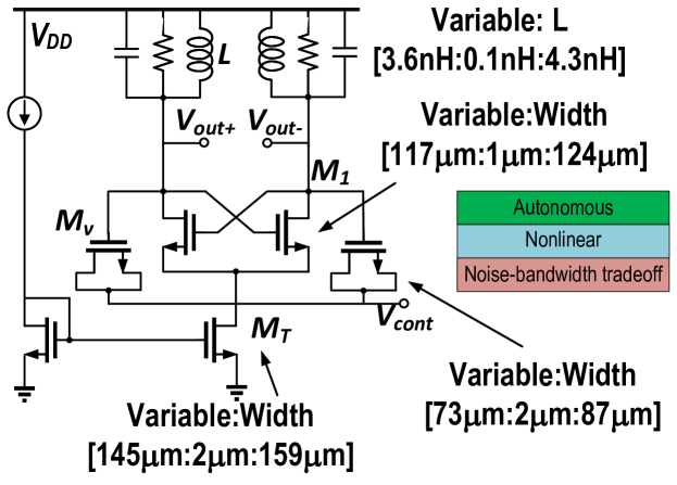
Figure 10: Schematic of a voltage-controlled oscillator (VCO).

5.3 Clustering Effect Analysis

Since our approach involves the replacement of circuit parameters with alternative parameters within the parameter space that yield improved performance, fewer distinct parameters remain after filtering than initially simulated. In situations where multiple performance metrics are mapped to the same parameter vector, it becomes intriguing to investigate the potential impact of this clustering on the performance of our algorithm. After constructing our dataset, we count the number of distinct circuits in the constructed dataset as well as the perplexity of the resulting dataset. The resulting perplexity is defined as $PP(p)=2^{H(p)}$ where entropy is estimated over the constructed dataset based on the counts of the distinct parameters. In the majority of circuits, the number of distinct parameter vectors in the constructed dataset is only approximately 3-12% of its size. In the majority of circuits, the number of distinct parameter vectors in the constructed dataset is only approximately 3-12% of its size. Specifically, for the Cascode circuit, we find 489 distinct circuits, which are 12% of the dataset size, while the resulting dataset’s perplexity is 286. In the case of more advanced circuits like Mixer and VCO, we observe a distinct count of 2-3% of the data size. The resulting perplexity is 45 for Mixer and 68 for VCO, both amounting to roughly 1% of their respective dataset sizes. The evident clustering effect observed in our construction method holds significant implications. One plausible hypothesis we put forward is that this clustering phenomenon could potentially be advantageous for training Machine Learning Models. By leveraging this clustering effect, we can effectively sidestep issues arising from overlapping mappings, enabling us to construct sample-efficient dataset.

5.4 Performance Metric Ordering Variations

In our study, we subjected the LNA circuit to an assessment using two distinct orders of performance metrics: Order A (Power Gain, $S_{11}$, NF), and Order B ($S_{11}$, NF, Power Gain). We optimized for maximizing Power Gain and minimizing $S_{11}$ and NF in both orders. Notably, the circuits generated by Order A showcased an average Power Gain that was larger (thus better) by 0.84 dB compared to those generated by Order B. Additionally, these circuits exhibited an average $S_{11}$ that was higher (thus worse) by 0.53 dB in comparison. We conducted a similar analysis for the Common Source Amplifier, Cascode Amplifier, and Two-Stage circuits. By prioritizing the order of the bandwidth during dataset construction, we observed circuits with higher average bandwidth. Similarly, with regards to power consumption, which we aimed to minimize, assigning the highest priority to power consumption led to the production of circuits with lower power consumption. We conclude that the user-specified order of performance metrics effectively creates the desired preference over them.

6 Conclusion

We present a data filtering pipeline that can generate, from a circuit simulation dataset, a training dataset for supervised learning of a circuit design agent for threshold specification. In extensive experiments with several baselines on a variety of linear, nonlinear, and autonomous analog and radio-frequency circuits, we find that our proposed method performs near-perfectly in all but the hardest circuit. This supports our hypothesis that a systematic selection of representative circuits can alleviate the “non-injective” property of the simulator function, which is vastly exacerbated by the threshold specification setting. The results also show the sample efficiency of our method. While not directly comparable with previous work, we often use a number of simulations an order of magnitude or more smaller than ever before, and learning from even 5% of this data is often highly successful as well. Lastly, we also show that our method is, to some extent, model agnostic by training with different machine learning methods and comparing their performance. To the best of our knowledge, this is the first time that a wide collection of analog circuits at various frequencies and of varied operations have been extensively examined and shown capable of being automatically designed. We believe that the methods and results of this work can help the growth of the circuit design industry by addressing the rapidly increasing demand for advanced electronic chipsets.

Appendix A Appendix

A.1 Model Architecture

In this work, we propose a Multi-layer perceptron (MLP) architecture with seven layers for the task at hand. The first layer takes in a vector of size equal to the number of performance metrics for the circuit and outputs a vector of length 200. The last layer takes in a vector of length 200 and outputs the same number of parameters as in the circuit. The middle five layers are constant across all circuits and have the following [input, output] size configurations: [200, 300], [300, 500], [500, 500], [500, 300], [300, 200]. Each layer is separated by the Rectified Linear Unit (ReLU) activation function. We trained each MLP model for 100 epochs using the Adam optimizer (Kingma & Ba, 2015) with a default learning rate of 0.001. Additionally, we also trained a Random Forest (RF) model with the default number of trees (100) and default arguments.

A.2 Comparing Methods

Figure 11: Comparing different ML methods in three circuits: (a) cascode; (b) low-noise amplifier; (c) voltage-controlled oscillator.

Figure 12: Comparing different ML methods in three circuits: (a) two stage; (b) mixer; and (c) power amplifier.

We compared the performance of three different machine learning methods: Neural Network (NN), Random Forest (RF), and Lookup Table (LT) using a ten-fold cross-validation setup with 90 % of the data used for training. The purpose of this work was to demonstrate that our method is model-agnostic, and thus, we did not attempt to fine-tune the NN or RF models. The lookup table approach was implemented by searching for the circuit with the lowest error in the training dataset for a given testing circuit. The NN and RF models were trained as specified in Section A.1. The results in table 1 suggest that all three methods perform similarly, with most of the circuits achieving 95-100% accuracy and a margin of 1%. This suggests that even a simple model like RF can produce good results. The detailed plots are presented in 12.

Table 1: Circuit Method Comparison at 1 $\%$

ML/Circuit	CS	Cascode	Two Stage	LNA	PA	Mixer	VCO
Lookup	0.94 $\pm$ 0.005	0.888 $\pm$ 0.005	0.961 $\pm$ 0.011	0.998 $\pm$ 0.001	0.958 $\pm$ 0.004	0.997 $\pm$ 0.001	0.833 $\pm$ 0.015
NN	0.854 $\pm$ 0.023	0.971 $\pm$ 0.004	0.964 $\pm$ 0.02	0.998 $\pm$ 0.0	0.945 $\pm$ 0.005	0.994 $\pm$ 0.001	0.847 $\pm$ 0.022
RF	0.953 $\pm$ 0.004	0.944 $\pm$ 0.005	1.0 $\pm$ 0.0	0.995 $\pm$ 0.001	0.95 $\pm$ 0.005	0.996 $\pm$ 0.001	0.853 $\pm$ 0.024

A.3 Comparing Datasizes

Table 2: Circuit Data Size Comparison for $D_{0}$ at 1 $\%$

%/Circuit	CS	Cascode	Two Stage	LNA	PA	Mixer	VCO
0.05	0.295 $\pm$ 0.036	0.207 $\pm$ 0.029	0.566 $\pm$ 0.04	0.944 $\pm$ 0.005	0.712 $\pm$ 0.026	0.319 $\pm$ 0.037	0.375 $\pm$ 0.033
0.1	0.278 $\pm$ 0.041	0.13 $\pm$ 0.025	0.676 $\pm$ 0.077	0.933 $\pm$ 0.012	0.711 $\pm$ 0.02	0.282 $\pm$ 0.055	0.342 $\pm$ 0.049
0.2	0.351 $\pm$ 0.047	0.292 $\pm$ 0.067	0.719 $\pm$ 0.078	0.991 $\pm$ 0.003	0.759 $\pm$ 0.029	0.364 $\pm$ 0.05	0.38 $\pm$ 0.089
0.5	0.54 $\pm$ 0.053	0.492 $\pm$ 0.065	0.813 $\pm$ 0.106	0.992 $\pm$ 0.007	0.689 $\pm$ 0.091	0.387 $\pm$ 0.021	0.452 $\pm$ 0.011
0.9	0.539 $\pm$ 0.051	0.583 $\pm$ 0.053	0.927 $\pm$ 0.022	0.998 $\pm$ 0.001	0.73 $\pm$ 0.014	0.396 $\pm$ 0.032	0.454 $\pm$ 0.055

Table 3: Circuit Data Size Comparison for $\bar{D}^{*}_{\epsilon}$ at 1 $\%$

%/Circuit	CS	Cascode	Two Stage	LNA	PA	Mixer	VCO
0.05	0.83 $\pm$ 0.018	0.803 $\pm$ 0.019	0.817 $\pm$ 0.021	0.972 $\pm$ 0.003	0.874 $\pm$ 0.026	0.927 $\pm$ 0.01	0.819 $\pm$ 0.009
0.1	0.751 $\pm$ 0.035	0.815 $\pm$ 0.029	0.962 $\pm$ 0.015	0.985 $\pm$ 0.003	0.927 $\pm$ 0.01	0.942 $\pm$ 0.013	0.82 $\pm$ 0.013
0.2	0.849 $\pm$ 0.029	0.886 $\pm$ 0.019	0.978 $\pm$ 0.004	0.991 $\pm$ 0.002	0.944 $\pm$ 0.013	0.969 $\pm$ 0.017	0.838 $\pm$ 0.019
0.5	0.917 $\pm$ 0.027	0.962 $\pm$ 0.009	0.938 $\pm$ 0.0	0.996 $\pm$ 0.003	0.963 $\pm$ 0.002	0.995 $\pm$ 0.002	0.814 $\pm$ 0.017
0.9	0.847 $\pm$ 0.04	0.971 $\pm$ 0.004	0.973 $\pm$ 0.018	0.997 $\pm$ 0.001	0.945 $\pm$ 0.006	0.995 $\pm$ 0.001	0.787 $\pm$ 0.037

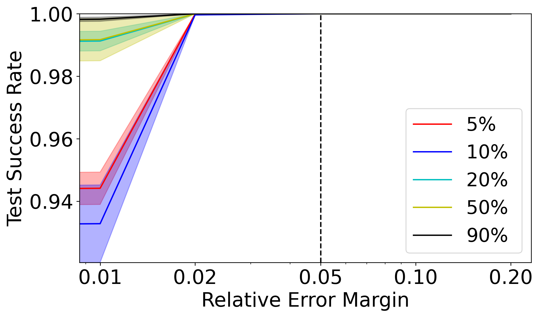
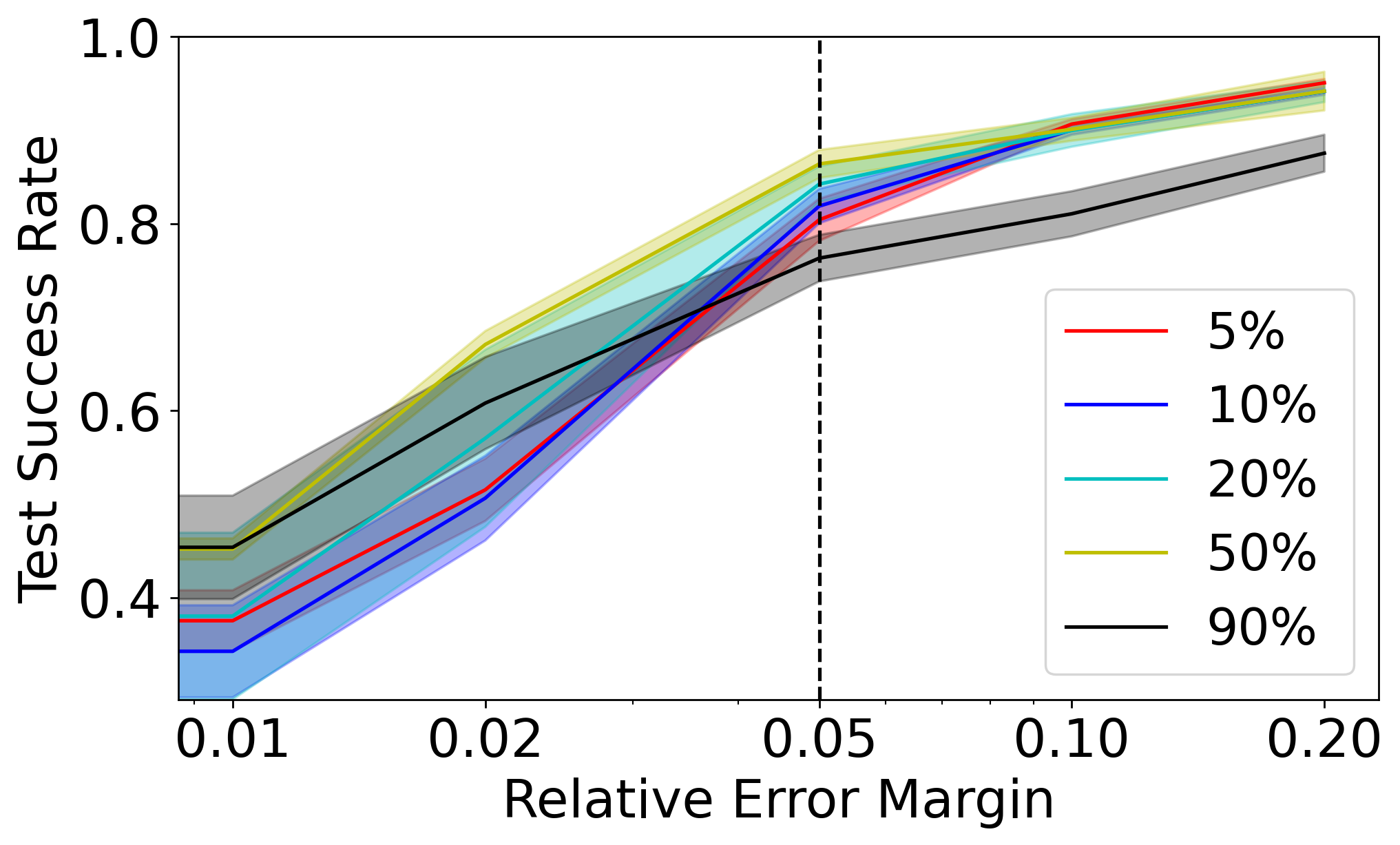
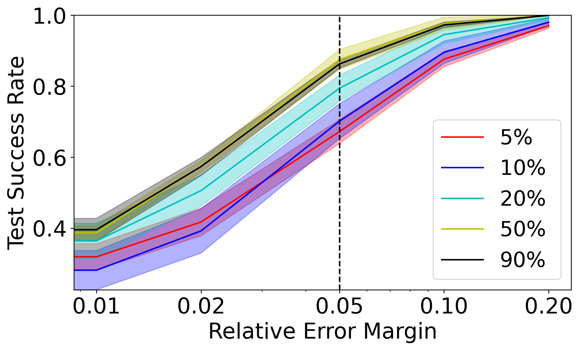
Figure 13: Comparing different datasizes for $D_{0}$ in circuits: (a) cascode; (b) low-noise amplifier (LNA); (c) voltage-controlled oscillator (VCO); (d) mixer.

Figure 14: Comparing different datasizes for $D_{0}$ in circuits: (a) common source amplifier (CS) ; (b) two-stage; (c) power amplifier (PA).

In this study, we assess the performance of various circuits by utilizing subsamples of varying sizes, including 5%, 10%, 20%, 50%, and 90% of the data. The 90% subsample corresponds to a range of 2700-3600 points, while the 5% subsample corresponds to approximately 150-200 points. Results indicate that the accuracy of the Two Stage circuit linearly increases from 56% to 93% as the subsample size increases from 5% to 90%. Similarly, for the $\bar{D_{\epsilon}^{*}}$ method, accuracy increases from 81% to 97%. Notably, all circuits exhibit an accuracy higher than 80%, even when using only 5% of the data. However, the accuracy of the $D_{0}$ circuit is observed to drop to 20% for certain subsamples.

A.4 Comparing Datasets

In addition to our previous results, we present a table of circuit evaluations for each method at a 1% margin. It can be observed that the Power Amplifier, VCO, and Mixer circuits achieve the highest scores when utilizing our method. However, for less complex circuits such as the Common Source Amplifier, the $D_{\epsilon}$ method yields a 2% higher score compared to our method.

Table 4: Circuit Comparison Info at 1 $\%$

D/Circuit	CS	Cascode	Two Stage	LNA	PA	Mixer	VCO
$D_{0}$	0.7 $\pm$ 0.036	0.519 $\pm$ 0.043	0.985 $\pm$ 0.01	0.996 $\pm$ 0.001	0.945 $\pm$ 0.005	0.486 $\pm$ 0.06	0.378 $\pm$ 0.054
$D_{\epsilon}$	0.957 $\pm$ 0.009	0.921 $\pm$ 0.033	0.99 $\pm$ 0.004	0.999 $\pm$ 0.0	0.97 $\pm$ 0.002	0.824 $\pm$ 0.019	0.713 $\pm$ 0.016
$D^{m}_{\epsilon}$	0.542 $\pm$ 0.014	0.435 $\pm$ 0.026	0.877 $\pm$ 0.033	0.976 $\pm$ 0.003	0.37 $\pm$ 0.048	0.32 $\pm$ 0.011	0.54 $\pm$ 0.021
$\bar{D}^{m}_{\epsilon}$	0.801 $\pm$ 0.038	0.578 $\pm$ 0.033	0.518 $\pm$ 0.048	0.8 $\pm$ 0.024	0.768 $\pm$ 0.092	0.401 $\pm$ 0.022	0.501 $\pm$ 0.015
$\bar{D}^{*}_{0}$	0.847 $\pm$ 0.021	0.947 $\pm$ 0.019	0.984 $\pm$ 0.011	0.997 $\pm$ 0.001	0.943 $\pm$ 0.004	0.858 $\pm$ 0.025	0.827 $\pm$ 0.019
$\bar{D}^{*}_{\epsilon}$	0.936 $\pm$ 0.012	0.962 $\pm$ 0.007	0.981 $\pm$ 0.012	0.998 $\pm$ 0.001	0.948 $\pm$ 0.005	0.995 $\pm$ 0.001	0.835 $\pm$ 0.016

A.5 Comparing Circuits

As seen in Table 7, a comparison of our proposed method is conducted against previous methods. However, due to the lack of standard benchmarks for circuits and limited data availability for many circuits, it should be noted that this comparison should be viewed as a general guide rather than a comprehensive evaluation. Nonetheless, it can be observed that our method demonstrates superior performance in comparison to previous methods, while also maintaining a small data size.

For each circuit, we also provide the following additional information:

1. The size of the train dataset, number of parameters, number of points per parameter in Table 6,

2. Average performance error across all the circuits in Table 5,

3. Performance metric range for every circuit in Table 8,9,

4. Parameters range for every circuit in Table 10.

Table 5: Average performance error $\%$ for every circuit using $\bar{D}^{*}_{\epsilon}$

Err/Circuit	CS	Cascode	Two Stage	LNA	PA	Mixer	VCO
Mean Error	0.06 $\pm$ 0.0	0.04 $\pm$ 0.0	0.03 $\pm$ 0.0	0.0 $\pm$ 0.0	1.29 $\pm$ 0.002	0.01 $\pm$ 0.0	1.13 $\pm$ 0.002

Table 6: Circuit complexity comparison

Circuit	CS	Cascode	Two-Stage	LNA	PA	Mixer	VCO
train-data size	3340	4080	616	4096	3528	3136	4096
Number of Parameters	2	3	3	4	4	3	4
Points per parameter	1670	1360	205.3	1024	882	1045.3	1024

Table 7: Comparing Results with the previous work

	Performance Metric	This Work (%)	Best Reported (%)	Related Works
CS	Gain	0.135$\pm$0.035	$<2.6$	Devi et al. (2021)
	Bandwidth	0.048 $\pm$ 0.12
	Power Consumption	0.0044$\pm$ 0.002
Cascode	Gain	0.0471$\pm$0.02	$\approx$ 1	Lourenço et al. (2019) Mina et al. (2022)
	Bandwidth	0.0433$\pm$0.01
	Power Consumption	0.0222$\pm$0.007
2-Stage	Gain	0.0226$\pm$0.018	1.1	Fukuda et al. (2017a)
	Bandwidth	0.00001 $\pm$ 0.000003	NA
	Power Consumption	0.0716$\pm$0.031	3.7	M.V. & Harish (2020a)
LNA	$G_{T}$	0.0028$\pm$0.001	$<$ 5	Dumesnil et al. (2014)
	$S_{11}$	0.007$\pm$0.001
	NF	0.002$\pm$0.0005
PA	Power Gain	1.207 $\pm$ 0.14	NA	NA
	Drain Efficiency	1.361 $\pm$ 0.2
	PAE	1.30 $\pm$ 0.19
Mixer	Conversion Gain	0.005$\pm$0.0035	NA	NA
	Power Consumption	0.86$\pm$0.002
	Swing	0.66$\pm$ 0.005
VCO	Power Consumption	0.017$\pm$ 0.1423	NA	NA
	Output Power	0.1423$\pm$0.01
	Tuning Range	3.226$\pm$0.6293

Table 8: Range of Analog Voltage Amplifiers Performance Metrics

Performance Metric	CS		Cascode		Two-Stage
	Min	Max	Min	Max	Min	Max
Gain (db)	5.25	15.14	20.94	28.23	41.28	73.82
Bandwidth (Hz)	83.7M	5.99G	2.17G	8.5G	12.1M	1.01G
Power Consumption (mW)	0.57	1.34	0.38	0.56	1.32	2.00

Table 9: Range of Non-linear Circuits Performance Metrics

	Performance Metric	Min	Max
LNA	Power Gain(db)	12.76	15.8
	$S_{11}$	-19.1	-17.3
	NF(db)	2.154	2.39
PA	Power Gain (db)	5.165	18.65
	Drain Efficiency (%)	9.39	33.92
	PAE(%)	3.79	28.67
Mixer	Conversion Gain	0.61	5.95
	Power Consumption (mW)	0.11	7.32
	Swing (mV)	0.61	5.95
VCO	Power Consumption (mW)	3.9	12.3
	Output Power(mW)	5.11	19.67
	Tuning Range (Hz)	451K	440M

Table 10: Design Parameters and Range of Variations

Circuit	Variable	Start	Step	End
CS	$M_{1}$[w]	2.8um	0.2um	6.6um
	$R_{D}$	620$\Omega$	5$\Omega$	1450$\Omega$
Cascode	$M_{1}$ [w]	8um	0.25um	11.5um
	$M_{2}$ [w]	2um	0.2um	5um
	$R_{D}$	9k$\Omega$	125$\Omega$	11k$\Omega$
Two-Stage	$M_{1}$[w]	25um	0.5um	30um
	$M_{2}$[w]	52um	0.5um	55.5um
	$M_{T}$[w]	6um	0.5um	9um
LNA	$M_{1,2}$[w]	73um	0.5um	76.5um
	$L_{g}$	9.4nH	0.2nH	10.8nH
	$L_{s}$	747pH	1pH	754pH
	$L_{d}$	3.7nH	0.1nH	4.4nH
PA	$M_{1,2,3,4}$[w]	18um	0.5um	22um
	$M_{5,6,7,8}$[w]	27um	1um	34um
	$V_{b1}$	785mV	5mV	815mV
	$V_{b2}$	760mV	5mV	790mV
Mixer	$M_{1}$[w]	8.55um	0.45um	11.7um
	$M_{T}$[w]	17.1um	0.9um	23.4um
	$V_{RF,DC}$	630mV	30mV	810mV
	R	240 $\Omega$	40$\Omega$	520$\Omega$
VCO	$M_{1}$[w]	8.55um	0.45um	11.7um
	$M_{T}$[w]	145um	2um	159um
	$M_{V}$[w]	73um	2um	87um
	L	3.6nH	0.1nH	4.3nH

References

- Abbasi et al. (2010) Abbasi, M., Kjellberg, T., de Graauw, A., van der Heijden, E., Roovers, R., and Zirath, H. A broadband differential cascode power amplifier in 45 nm cmos for high-speed 60 ghz system-on-chip. In 2010 IEEE Radio Frequency Integrated Circuits Symposium, pp. 533–536. IEEE, 2010.
- Afacan et al. (2021) Afacan, E., Lourenço, N., Martins, R., and Dündar, G. Machine learning techniques in analog/rf integrated circuit design, synthesis, layout, and test. Integration, 77:113–130, 2021.
- Bandler & Chen (1988) Bandler, J. and Chen, S. Circuit optimization: the state of the art. IEEE Transactions on Microwave Theory and Techniques, 36(2):424–443, 1988. doi: 10.1109/22.3532.
- Bandler & Rayas-Sánchez (2023) Bandler, J. W. and Rayas-Sánchez, J. E. An early history of optimization technology for automated design of microwave circuits. IEEE Journal of Microwaves, 3(1):319–337, 2023. doi: 10.1109/JMW.2022.3225012.
- Boyd et al. (2005) Boyd, S. P., Kim, S.-J., Patil, D. D., and Horowitz, M. A. Digital circuit optimization via geometric programming. Operations research, 53(6):899–932, 2005.
- Breiman (2001) Breiman, L. Random forests. Machine learning, 45(1):5–32, 2001.
- Brunvand (2010) Brunvand, E. Digital VLSI chip design with Cadence and Synopsys CAD tools. Addison-Wesley New York, 2010.
- Dai & Harjani (2003) Dai, L. and Harjani, R. Design of high-performance CMOS voltage-controlled oscillators. Springer Science & Business Media, 2003.
- Devi et al. (2021) Devi, S., Tilwankar, G., and Zele, R. Automated design of analog circuits using machine learning techniques. In 2021 25th International Symposium on VLSI Design and Test (VDAT), pp. 1–6, 2021. doi: 10.1109/VDAT53777.2021.9601131.
- Dumesnil et al. (2014) Dumesnil, E., Nabki, F., and Boukadoum, M. Rf-lna circuit synthesis by genetic algorithm-specified artificial neural network. In 2014 21st IEEE International Conference on Electronics, Circuits and Systems (ICECS), pp. 758–761, 2014. doi: 10.1109/ICECS.2014.7050096.
- Fukuda et al. (2017a) Fukuda, M., Ishii, T., and Takai, N. Op-amp sizing by inference of element values using machine learning. In 2017 International Symposium on Intelligent Signal Processing and Communication Systems (ISPACS), pp. 622–627, 2017a. doi: 10.1109/ISPACS.2017.8266553.
- Fukuda et al. (2017b) Fukuda, M., Ishii, T., and Takai, N. Op-amp sizing by inference of element values using machine learning. In 2017 International Symposium on Intelligent Signal Processing and Communication Systems (ISPACS), pp. 622–627, 2017b. doi: 10.1109/ISPACS.2017.8266553.
- Gilbert (1968) Gilbert, B. A precise four-quadrant multiplier with subnanosecond response. IEEE Journal of Solid-State Circuits, 3(4):365–373, 1968. doi: 10.1109/JSSC.1968.1049925.
- Gray & Meyer (1982) Gray, P. R. and Meyer, R. G. Mos operational amplifier design-a tutorial overview. Ieee journal of solid-state circuits, 17(6):969–982, 1982.
- Grover & Chaudhary (2014) Grover, G. and Chaudhary, I. Implementation of particle swarm optimization algorithm in vhdl for digital circuits optimization. International Journal of Information Engineering and Electronic Business, 6(5):16, 2014.
- Hajimiri & Lee (1999) Hajimiri, A. and Lee, T. H. Design issues in cmos differential lc oscillators. IEEE Journal of Solid-State Circuits, 34(5):717–724, 1999.
- Harsha & Harish (2020) Harsha, M. and Harish, B. Artificial neural network model for design optimization of 2-stage op-amp. In 2020 24th International Symposium on VLSI Design and Test (VDAT), pp. 1–5. IEEE, 2020.
- Hassan et al. (2016) Hassan, A.-K. S., Mohamed, A. S., Rabie, A. A., and Etman, A. S. A novel surrogate-based approach for optimal design of electromagnetic-based circuits. Engineering Optimization, 48(2):185–198, 2016.
- Kamal (2022) Kamal, K. Y. The silicon age: Trends in semiconductor devices industry. Journal of Engineering Science & Technology Review, 15(1), 2022.
- Kingma & Ba (2015) Kingma, D. P. and Ba, J. Adam: A method for stochastic optimization. In ICLR (Poster), 2015. URL http://arxiv.org/abs/1412.6980.
- Ko & Lin (2006) Ko, S. and Lin, J. A linearized cascode cmos power amplifier. In 2006 IEEE Annual Wireless and Microwave Technology Conference, pp. 1–4. IEEE, 2006.
- Kouhalvandi et al. (2018) Kouhalvandi, L., Ceylan, O., and Yagci, H. B. Power amplifier design optimization with simultaneous cooperation of eda tool and numeric analyzer. In 2018 18th Mediterranean Microwave Symposium (MMS), pp. 202–205. IEEE, 2018.
- Kunz & Pradhan (1994) Kunz, W. and Pradhan, D. K. Recursive learning: a new implication technique for efficient solutions to cad problems-test, verification, and optimization. IEEE Transactions on Computer-Aided Design of Integrated Circuits and Systems, 13(9):1143–1158, 1994.
- Lannutti et al. (2012) Lannutti, F., Nenzi, P., and Olivieri, M. Klu sparse direct linear solver implementation into ngspice. In Proceedings of the 19th International Conference Mixed Design of Integrated Circuits and Systems-MIXDES 2012, pp. 69–73. IEEE, 2012.
- Lerdworatawee & Namgoong (2005) Lerdworatawee, J. and Namgoong, W. Wide-band cmos cascode low-noise amplifier design based on source degeneration topology. IEEE Transactions on Circuits and Systems I: Regular Papers, 52(11):2327–2334, 2005.
- Lourenço et al. (2018) Lourenço, N., Rosa, J., Martins, R., Aidos, H., Canelas, A., Póvoa, R., and Horta, N. On the exploration of promising analog ic designs via artificial neural networks. In 2018 15th International Conference on Synthesis, Modeling, Analysis and Simulation Methods and Applications to Circuit Design (SMACD), pp. 133–136. IEEE, 2018.
- Lourenço et al. (2018) Lourenço, N., Rosa, J., Martins, R., Aidos, H., Canelas, A., Póvoa, R., and Horta, N. On the exploration of promising analog ic designs via artificial neural networks. In 2018 15th International Conference on Synthesis, Modeling, Analysis and Simulation Methods and Applications to Circuit Design (SMACD), pp. 133–136, 2018. doi: 10.1109/SMACD.2018.8434896.
- Lourenço et al. (2019) Lourenço, N., Afacan, E., Martins, R., Passos, F., Canelas, A., Póvoa, R., Horta, N., and Dundar, G. Using polynomial regression and artificial neural networks for reusable analog ic sizing. In 2019 16th International Conference on Synthesis, Modeling, Analysis and Simulation Methods and Applications to Circuit Design (SMACD), pp. 13–16, 2019. doi: 10.1109/SMACD.2019.8795282.
- Martin (2002) Martin, A. J. L. Cadence design environment. New Mexico State University, Tutorial paper, pp. 35, 2002.
- Micheli (1994) Micheli, G. D. Synthesis and optimization of digital circuits. McGraw-Hill Higher Education, 1994.
- Mina et al. (2022) Mina, R., Jabbour, C., and Sakr, G. E. A review of machine learning techniques in analog integrated circuit design automation. Electronics, 11(3):435, 2022.
- Murphy & McCarthy (2021) Murphy, S. D. and McCarthy, K. G. Automated design of cmos operational amplifier using a neural network. In 2021 32nd Irish Signals and Systems Conference (ISSC), pp. 1–6. IEEE, 2021.
- M.V. & Harish (2020a) M.V., H. and Harish, B. P. Artificial neural network model for design optimization of 2-stage op-amp. In 2020 24th International Symposium on VLSI Design and Test (VDAT), pp. 1–5, 2020a. doi: 10.1109/VDAT50263.2020.9190315.
- M.V. & Harish (2020b) M.V., H. and Harish, B. P. Artificial neural network model for design optimization of 2-stage op-amp. In 2020 24th International Symposium on VLSI Design and Test (VDAT), pp. 1–5, 2020b. doi: 10.1109/VDAT50263.2020.9190315.
- Nenzi & Vogt (2011) Nenzi, P. and Vogt, H. Ngspice users manual version 23, 2011.
- Niknejad et al. (2012) Niknejad, A. M., Chowdhury, D., and Chen, J. Design of cmos power amplifiers. IEEE Transactions on Microwave Theory and Techniques, 60(6):1784–1796, 2012.
- Razavi (2012) Razavi, B. RF microelectronics, volume 2. Prentice hall New York, 2012.
- Renner & Ekárt (2003) Renner, G. and Ekárt, A. Genetic algorithms in computer aided design. Computer-aided design, 35(8):709–726, 2003.
- Settaluri et al. (2020) Settaluri, K., Haj-Ali, A., Huang, Q., Hakhamaneshi, K., and Nikolic, B. Autockt: Deep reinforcement learning of analog circuit designs. In 2020 Design, Automation & Test in Europe Conference & Exhibition (DATE), pp. 490–495. IEEE, 2020.
- Vural et al. (2015) Vural, R., Kahraman, N., Erkmen, B., and Yildirim, T. Process independent automated sizing methodology for current steering dac. International Journal of Electronics, 102(10):1713–1734, 2015.
- Wang et al. (2018a) Wang, H., Yang, J., Lee, H.-S., and Han, S. Learning to design circuits. arXiv preprint arXiv:1812.02734, 2018a.
- Wang et al. (2018b) Wang, Z., Luo, X., and Gong, Z. Application of deep learning in analog circuit sizing. In Proceedings of the 2018 2nd International Conference on Computer Science and Artificial Intelligence, CSAI ’18, pp. 571–575, New York, NY, USA, 2018b. Association for Computing Machinery. ISBN 9781450366069. doi: 10.1145/3297156.3297160. URL https://doi.org/10.1145/3297156.3297160.