Modeling the Chromosphere and Transition Region of Planet-hosting Star GJ 436

Abstract

Ahead of upcoming space missions intending to conduct observations of low-mass stars in the ultraviolet (UV) spectral region it becomes imperative to simultaneously conduct atmospheric modeling from the UV to the visible (VIS) and near-infrared (NIR). Investigations on extended spectral regions will help to improve the overall understanding of the diversity of spectral lines arising from very different atmospheric temperature regions. Here we investigate atmosphere models with a chromosphere and transition region for the M2.5V star GJ 436, which hosts a close-in Hot Neptune. The atmosphere models are guided by observed spectral features from the UV to the VIS/NIR originating in the chromosphere and transition region of GJ 436. High-resolution observations from the Hubble Space Telescope and Calar Alto high-Resolution search for M dwarfs with Exo-earths with Near-infrared and optical Echelle Spectrographs (CARMENES) are used to obtain an appropriate model spectrum for the investigated M dwarf. We use a large set of atomic species considered in nonlocal thermodynamic equilibrium conditions within our PHOENIX model computations to approximate the physics within the low-density atmospheric regions. In order to obtain an overall match for the nonsimultaneous observations, it is necessary to apply a linear combination of two model spectra, where one of them better reproduces the UV lines while the other better represents the lines from the VIS/NIR range. This is needed to adequately handle different activity states across the observations.

1 Introduction

Modeling the lowest-density regions of stellar atmospheres, from the chromosphere to corona (also referred to as the upper atmosphere in the following), remains a challenging exercise. Processes such as acoustic heating (Wedemeyer et al., 2004), ambipolar diffusion, and conduction (Fontenla et al., 1990, 1991, 1993) are believed to contribute to the nonradiative heating in the upper atmosphere, but incorporating these into a self-consistent atmosphere model remains difficult given the range of densities and temperatures. Using semiempirical one-dimensional temperature structures, as first used for modeling different regions on the surface of the Sun (Vernazza et al., 1973, 1981), turned out to be highly effective in computing synthetic spectra that match spectral lines arising from its upper atmosphere. Atmosphere codes such as PHOENIX (Hauschildt, 1992, 1993; Hauschildt & Baron, 1999) can take into account the upper atmosphere, i. e., the chromosphere and transition region (designating the steep rise in temperature between chromosphere and corona), and have been proven capable of reproducing observed chromosphere and transition region lines of M-dwarf stars from the ultraviolet (UV) (e. g., Peacock et al., 2019a, b) to the visible (VIS) and near-infrared (NIR) wavelength ranges (e. g., Hintz et al., 2019, 2020).

The M2.5V star GJ 436 and its closely orbiting Hot Neptune GJ 436b have been continuously in the spotlight of scientific investigations throughout the last two decades. GJ 436 is located 9.78 pc away from the Sun (Gaia Collaboration et al., 2021) and has a radius of 0.42 $R_{\odot}$ and a mass of 0.44 $M_{\odot}$ (Rosenthal et al., 2021). This M-dwarf star exhibits periodic variations on short- and long-term scales. The rotational period of 44.6 days (Díez Alonso et al., 2019) and an activity cycle of about 7.4 yr (Lothringer et al., 2018) have been detected from photometric variations. Chromospheric activity indicators have been found to vary on similar timescales due to rotation (Suárez Mascareño et al., 2015) and the activity cycle (Kumar & Fares, 2023). GJ 436b orbits its host star at 0.03 au with an orbital period of 2.64 days (Butler et al., 2004) and it is well known that high-energy radiation, from the host star in the UV and X-ray range, can significantly influence the atmosphere of exoplanets (e. g., Lammer et al., 2007; Tian et al., 2008). Due to the close orbit of GJ 436b, the high-energy radiation from GJ 436 strongly influences the Hot Neptune’s atmosphere and drives its atmospheric evolution (Kulow et al., 2014; Ehrenreich et al., 2015; Bourrier et al., 2016). From extensive and continued observations of GJ 436 and access to precise transmission spectroscopy of GJ 436b, it becomes essential to study the low-density part of the atmosphere of the host star in order to better understand the characteristics of GJ 436 and, eventually, to improve our understanding of GJ 436b.

Stellar activity is a common property of M-dwarf stars and there are a number of spectral lines that are sensitive to this activity as well as to the temperatures across the upper atmospheric layers (Vernazza et al., 1981; Fontenla et al., 1990; Andretta & Jones, 1997; Fuhrmeister et al., 2005). In particular, the hydrogen H$\alpha$ line at 6564.6 $\AA$ (vacuum wavelength), and located in the visible part of the spectrum, is a valuable and often-used activity indicator (e. g., Stauffer & Hartmann, 1986; Gizis et al., 2002; Robertson et al., 2016). However, this line exhibits an ambiguous behavior in the low-activity regime, i. e., with increasing stellar activity, the absorption depth increases before filling in and reversing into an emission line with even stronger activity states (Cram & Mullan, 1979). This complicated behavior can lead to misinterpretation, and so various chromospheric lines should be considered when studying stellar activity and related atmospheric properties. The chromospheric lines of the Ca II infrared triplet (IRT) ($\lambda\lambda=$ 8500.4, 8544.4, 8664.5 $\AA$) and Na I D doublet ($\lambda\lambda=$ 5891.6, 5897.6 $\AA$) constitute other tracers used for activity-related investigations (e. g., Gomes da Silva et al., 2011; Martínez-Arnáiz et al., 2011; Robertson et al., 2016; Martin et al., 2017). While the H$\alpha$ line is formed in the upper chromosphere, the Ca II IRT and Na I D lines can be used to characterize the lower chromosphere (e. g., Hintz et al., 2019). The He I IRT lines ($\lambda\lambda=$ 10 832.1, 10 833.2, 10 833.3 $\AA$) are sensitive to temperatures from around 10 000 to 20 000 K and therefore are good probes of the base of the transition region (e. g., Andretta & Giampapa, 1995; Andretta & Jones, 1997; Hintz et al., 2020). Their line formation is actually dependent on the nonlocal UV continuum shortward of 504 $\AA$ which is capable of ionizing the neutral helium in the first place before the line’s lower energy level can be populated by electrons (e. g., Andretta & Giampapa, 1995; Andretta & Jones, 1997; Hintz et al., 2020). This highlights the necessity of further extending stellar atmosphere modeling by taking into account broad wavelength ranges from the UV to the NIR region. The He I IRT lines are also often used to measure and investigate the atmospheres of exoplanets while transiting their host stars (Allart et al., 2018; Nortmann et al., 2018; Salz et al., 2018; Spake et al., 2018).

The hydrogen Ly$\alpha$ line ($\lambda=$ 1215.7 $\AA$), which contributes a significant portion of flux to the UV part of the spectrum, is used to study the shape of the transition region and considered a proxy for the often inaccessible extreme UV (EUV) wavelength range (e. g., Linsky et al., 2014; Peacock et al., 2019a). Furthermore, irradiation from Ly$\alpha$ is also known to influence the composition of planetary atmospheres (e. g., Vidal-Madjar et al., 2004; Trainer et al., 2006). The C IV lines at 1550 $\AA$ are also relatively strong lines originating from the transition region and are formed at even higher temperatures than Ly$\alpha$ (Linsky, 2017). Both of these lines have previously been used to model the transition region (e. g., Peacock et al., 2019a, b). The lines discussed above are all sensitive to different atmospheric regions and thus will provide the empirical guidance we need to construct a model atmosphere capable of reproducing the overall UV through IR spectrum of GJ436.

GJ 436 has already been the subject of stellar atmosphere modeling in the UV (Peacock et al., 2019b) as well as in the VIS and NIR (Hintz et al., 2019, 2020) wavelength regions. Both studies used the PHOENIX code to obtain appropriate models to reproduce the spectral features considered. These studies modeled the UV and VIS/NIR lines seperately, the work of this paper models these regions simultaneously to obtain an overall match to the observations.

Section 2 gives an overview about how the PHOENIX models are constructed and important model properties. Thereupon, we compare our synthetic spectra to GJ 436 observations (Section 3) obtained from the Hubble Space Telescope (HST) for the UV region and from the Calar Alto high-Resolution search for M dwarfs with Exo-earths with Near-infrared and optical Echelle Spectrographs (CARMENES; Quirrenbach et al., 2018) for the VIS/NIR range. Finally, in Section 4 we summarize our results and give a conclusion of this work.

2 Model construction

For our modeling of GJ 436, we use the stellar atmosphere code PHOENIX (Hauschildt, 1992, 1993; Hauschildt & Baron, 1999). The PHOENIX code has the capability to compute the synthetic spectrum based on a given semiempirical, ad hoc 1D temperature structure (Fuhrmeister et al., 2005) where we are able to specify the temperature structure of the chromosphere and transition region and include a nonlocal thermodynamic equilibrium (NLTE) treatment of many atomic and ion species. The PHOENIX code is still the subject of further ongoing improvements: for instance the work by Peacock et al. (2019a, b) recently added a partial frequency redistribution mode (Hubeny & Lites, 1995; Uitenbroek, 2001) in order to better match observed resonance lines such as the Ly$\alpha$ line in the UV spectra of a few M dwarfs. This makes the PHOENIX code a good choice to create model spectra for spectral lines that are observed in late-type stars and form in the upper atmospheres of these stars.

By introducing free parameters that determine the atmospheric position of the temperature minimum or the top of the chromosphere (see, e. g., Hintz et al., 2019; Peacock et al., 2019a, for a detailed description), we construct such a semiempirical, ad hoc 1D temperature structure representing the chromosphere and transition region. On top of the basic photosphere model (with the stellar parameters of GJ 436 as given in Table 2) we attach an atmospheric structure with temperatures increasing outwards up to $\sim$200 000 K.

In Fig 1, we show two example atmosphere temperature structures we considered in this paper. The depicted models M1 and M2 differ by the onset of the transition region in terms of the column mass density – M1’s transition region is located at $m=-5.2\,$dex while for M2 it is $m=-5.0\,$dex. In Fig 1, we also indicate the temperature regions of M2 where the majority of flux emerges for spectral lines discussed in this work. These temperature ranges were determined from the flux contribution function (Magain, 1986; Fuhrmeister et al., 2006) and following the method described by Hintz et al. (2019). A line formation analysis is beyond the scope of this paper (for this, see, e. g., Falchi & Mauas, 1998); however, with this we can get an impression about the temperature regions responsible in the chromosphere and transition region. The onset of the transition region of model M2 is located at a density almost $\sim$1.6 times larger than in the case of model M1.

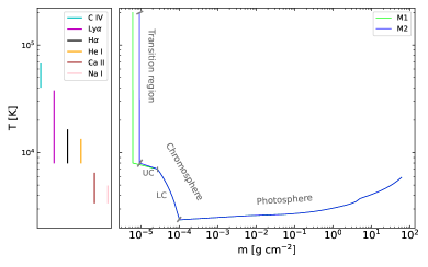
Figure 1: Temperature profiles of models M1 (green) and M2 (blue) as a function of column mass density (right panel). On the left-hand side, we indicate approximate atmospheric temperatures above the temperature minimum where most of the line fluxes of Ly$\alpha$, C IV, H$\alpha$, He I IRT, Ca II IRT, and Na I D₂ in model M2 originate from according to the flux contribution function (Magain, 1986; Fuhrmeister et al., 2006; Hintz et al., 2019). The corresponding temperature regions of M1 are similar. For the Ca II IRT and Na I D₂ lines, they are actually the same, while they are slightly lower for the other lines, but $\sim$2500 K at most. For M2 we indicate by gray lines the boundaries of the transition region and upper (UC) and lower chromosphere (LC), as well as the photosphere.

Using different increases in temperature at different atmospheric heights follows a well-known approach already tested and applied to M dwarfs by several former model studies of the Sun and M dwarfs (e. g., Vernazza et al., 1981; Andretta & Jones, 1997; Fuhrmeister et al., 2005). Furthermore, the general shape of this temperature structure is similar to the one obtained for the Sun by balancing radiative losses and the nonradiative heating mechanisms of thermal conduction and ambipolar diffusion as introduced by Fontenla et al. (1990, 1991, 1993). However, the steep temperature gradient of the transition region simulates the conduction mostly responsible for the energy transport at these heights (Fuhrmeister et al., 2005) and turned out to be an appropriate model approximation up to a temperature of 200 000 K (Peacock et al., 2019a, b).

Table 1: Spectral observations of GJ 436 used for the considered spectral features.

Spectral Feature	Wavelengths [$\AA$]	Spectrograph	Average Resolving Power	Observation Date	References
Ly${\alpha}$	1215.7	HST/STIS	14 400	2015 Jun 24	1, 2, 3
C IV	1548.2	HST/COS	16 500	2015 Jun 25	1, 2, 3
NUV	2000–3000	HST/STIS	3000	2015 Jun 24	1, 2, 3
Na I D2	5891.6	CARMENES/VIS	94 600	2016 Jan 8 - 2016 Nov 20	4
H$\alpha$	6564.6	CARMENES/VIS	94 600	2016 Jan 8 - 2016 Nov 20	4
Ca II IRT	8500.4	CARMENES/VIS	94 600	2016 Jan 8 - 2016 Nov 20	4
He I IRT	10 833.3	CARMENES/NIR	80 400	2016 Jan 8 - 2016 Nov 20	4

Table 2: Stellar parameters of GJ 436.

Parameter	Value	Reference
M⋆ [M⊙]	0.441 $\pm$ 0.009	1
R⋆ [R⊙]	0.417 $\pm$ 0.008	1
d [pc]	9.775 $\pm$ 0.003	2
SpT	M2.5	3
Teff [K]	3533 $\pm$ 26	4
logg [dex]	4.83	4
vrad [km/s]	9.59 $\pm$ 0.001	5

Recent studies of M-dwarf stars using such 1D ad hoc temperature structures in the upper atmosphere were able to adequately match chromospheric and transition region lines of H$\alpha$, Ca II IRT, Na I D, and He I IRT in the VIS and NIR wavelength ranges in high-resolution spectra (Hintz et al., 2019, 2020). Furthermore, such models could also be used to successfully reproduce spectral lines of Ly$\alpha$ and Mg II in the UV wavelength range of M-dwarf stars (Peacock et al., 2019a, b).

In the upper atmosphere where the temperature strongly increases and the atmosphere becomes optically thin, it is necessary to account for NLTE conditions when treating the most abundant atomic and ion species. Therefore, the following elements are computed in NLTE: H i, He i-ii, C i-iv, N i-v, O i-v, Ne i-ii, Na i-iii, Mg i-iv, Al i-iv, Si i-iv, P i-ii, S i-iii, Cl i-iii, Ar i-iii, K i-iii, Ca i-iii, Ti i-iv, V i-iii, Cr i-iii, Mn i-iii, Fe i-iv, Co i-iii, and Ni i-iii. We treat a total of 74 species in NLTE; for most of them we use level data provided by PHOENIX (Kurucz & Bell, 1995), but for He i-ii and C IV we use the CHIANTI V7 (Landi et al., 2013) database. As suggested by Fuhrmeister et al. (2006), we do not include LTE background lines when treating hydrogen in NLTE.

In addition to electron collisions we employ hydrogen collisional rates according to the empirical findings of Drawin (1968, 1969), which are important for the formation of line wings where hydrogen densities are orders of magnitude higher than electron densities (Barklem, 2007). This particularly accounts for a correct treatment of the atmospheric region around the temperature minimum where collisions are generally still important but the electron density is comparably low. Further details about the model construction are available in Hintz et al. (2019) and Peacock et al. (2019a).

3 Comparison to observations

In this work we use spectral observations from the HST taken from the Measurements of the Ultraviolet Spectral Characteristics of Low-mass Exoplanetary Systems Treasury Survey (MUSCLES; France et al., 2016; Youngblood et al., 2016; Loyd et al., 2016) to analyze UV lines of GJ 436. For investigating the VIS and NIR region of GJ 436, we use spectral observations from CARMENES (Quirrenbach et al., 2018). Due to a high level of telluric contamination in the NIR region around the He I IRT lines we use the CARMENES coadded template spectrum obtained from the CARMENES reduction pipeline (Zechmeister et al., 2018; Nagel, 2019). The considered HST observations were taken in 2015 June while the CARMENES observations cover the period from 2016 January to 2016 November.

Investigating possible long-term cycles within the CARMENES data, Fuhrmeister et al. (2023) did not find any activity-related trend for GJ 436. Yet, apart from CARMENES data, they could detect an $R^{\prime}_{\mathrm{HK}}$ long-term cycle over a period of more than 17 yr with variations of less than $\sim$20 % within the corresponding sinusoidal best fit of the $R^{\prime}_{\mathrm{HK}}$ modulation. Kumar & Fares (2023) reported long-term periodicities of H$\alpha$ and Na I indicators of $\sim$6 yr, which is in line with the detected photometric cycle (Lothringer et al., 2018; Loyd et al., 2023). The activity study by Hintz et al. (2019) included GJ 436, but could not find significant variations within the investigated chromospheric lines from the activity state. The time period of the observational data used from CARMENES only covers $\sim$1/6 of the reported H$\alpha$ and Na I indicator perodicities and $\sim$1/17 of the detected $R^{\prime}_{\mathrm{HK}}$ cycle. Therefore, we only use a small fraction of any of these and do not expect significantly strong variations within the time period of 2016 we use for our coadded CARMENES spectrum. Furthermore, we checked the considered lines in the coadded spectrum from CARMENES in timespans of $\sim 3$ and $\sim 6$ months for variations in 2016 and could not find significant changes, either. Thus, we consider it reasonable to use the averaged VIS/NIR CARMENES spectrum for our investigation.

We convolve our PHOENIX spectra to the spectral resolutions of the instruments in the respective wavelength ranges. HST spectra have a resolving power at the wavelengths of the Ly$\alpha$ and C IV lines of $\sim$14 400 and $\sim$16 500 respectively, while the resolving power is $\sim$94 600 in the CARMENES VIS channel (covering Na I D, H$\alpha$, Ca II IRT) and $\sim$80 400 in the NIR channel (He I IRT). Table 1 provides a summary of the considered spectral features and respective observations of GJ 436 used in this work. An overview of the stellar parameters of GJ 436 is given in Table 2.

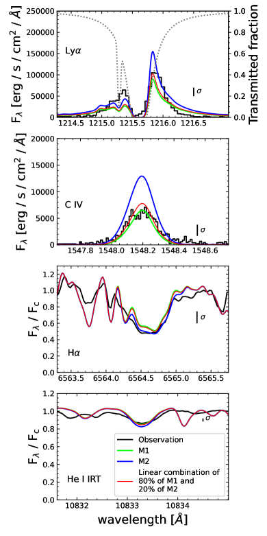
Figure 2: Models M1 and M2 (green and blue lines) obtained from the temperature structures depicted in Fig 1 (with corresponding color-coding) and observations (black lines) of GJ 436 shown in the lines of Ly$\alpha$ together with the ISM transmittance curve for GJ 436 provided by Youngblood et al. (2016, gray dashed line; an exemplary insight into how we apply the ISM transmission to our model M2 is provided in Appendix A) (top panel), C IV (second panel), H$\alpha$ (third panel), He I IRT (bottom panel). Red lines correspond to the best linear combinations of the model components M1 and M2. HST observations are scaled by d²/R${}_{\star}^{2}$ to the stellar surface. VIS/NIR lines of CARMENES observations and model spectra are continuum-normalized. The $\sigma$-values correspond to the standard deviations of the observed line flux (for Ly$\alpha$ $\sigma$ is calculated from the line wings only).

3.1 Single models

In order to find a chromospheric PHOENIX model in good agreement with UV and VIS/NIR observations of GJ 436, we use two spectral lines observed by HST representing the UV region as well as two lines from the VIS/NIR range observed by CARMENES. Therefore, we are using two lines to represent each wavelength region. The UV region is here represented by the lines of hydrogen Ly$\alpha$ at $1215.7\,\AA$ and C IV at $1548.2\,\AA$. When comparing our synthetic spectra to the observed Ly$\alpha$ line of GJ 436, we apply the interstellar medium (ISM) transmission curve as found by Youngblood et al. (2016) in order to compare our modeled Ly$\alpha$ line to what HST is actually able to observe with respect to the interstellar absorption along the line of sight. For the VIS/NIR wavelength range, we use two of the activity indicators also applied by Hintz et al. (2020) to find a matching model: the hydrogen H$\alpha$ line at $6564.6\,\AA$, and the strongest component of the He I IRT at $10\,833.3\,\AA$ which consists of the two red overlapping triplet lines. The blue component of the triplet at $10\,832.1\,\AA$ is not observable for this spectral type, but there may be stronger molecular lines in this wavelength region (Fuhrmeister et al., 2019).

In Figure 2, we show the observed lines as well as the modeled lines obtained from the atmosphere structures depicted in Figure 1. For the CARMENES observations, we normalize both the observations and model spectra to the local continua since the CARMENES spectra are not flux-calibrated. While the synthetic spectrum of model M1 better reproduces the C IV line ($\chi^{2}_{\mathrm{C\,IV,\mathrm{M1}}}=9.7$ compared to $\chi^{2}_{\mathrm{C\,IV,\mathrm{M2}}}=103.7$), M2 yields a better match for H$\alpha$ ($\chi^{2}_{\mathrm{H\alpha,\mathrm{M1}}}=12.8$ compared to $\chi^{2}_{\mathrm{H\alpha,\mathrm{M2}}}=5.1$). The situation in Ly$\alpha$ and the He I IRT is less clear, i. e., $\chi^{2}$-values of M1 and M2 differ by a factor of $\lesssim 2$ for these lines. Model M2 overpredicts C IV and the right Ly$\alpha$ wing, but matches H$\alpha$ and also the He I IRT. On the other hand, M1 fits C IV and the He I IRT, but underpredicts H$\alpha$ and the left Ly$\alpha$ wing. However, the shapes of all lines are reproduced by both models. We are investigating these lines since the UV lines in this selection represent the two strongest ones as measured by Peacock et al. (2019b) and the H$\alpha$ and He I IRT lines exhibit discrepancies between the two models. The Na I D₂ line at $5891.6\,\AA$ and the bluest Ca II IRT line at $8500.4\,\AA$, which have also been used in the modeling conducted by Hintz et al. (2020), are almost identical in the models M1 and M2 (see Figure B.2 in Appendix B).

Finding synthetic spectra that best match the observed lines involves modifying the parameters characterizing the densities and temperature rises of the chromosphere and transition region. However, significant departures from LTE often complicate the behavior of spectral lines with respect to changes in the temperatures structure. As discussed by Peacock et al. (2019a, b), the overall UV spectrum is very sensitive to the column mass density at the base of the transition region. However, individual lines respond differently, and in some cases with opposite trends with respect to changes in the temperature profile. For example, the H$\alpha$ line depends strongly on the structure of the upper chromosphere and lower transition region while the Ca II IRT lines are less affected by these atmospheric regions, and vice versa for the structure of the lower chromosphere (Hintz et al., 2019). However, H$\alpha$ is not independent of the structure of the lower chromosphere either, illustrating the difficulty of finding an appropriate model that simultaneously reproduces the different line observations.

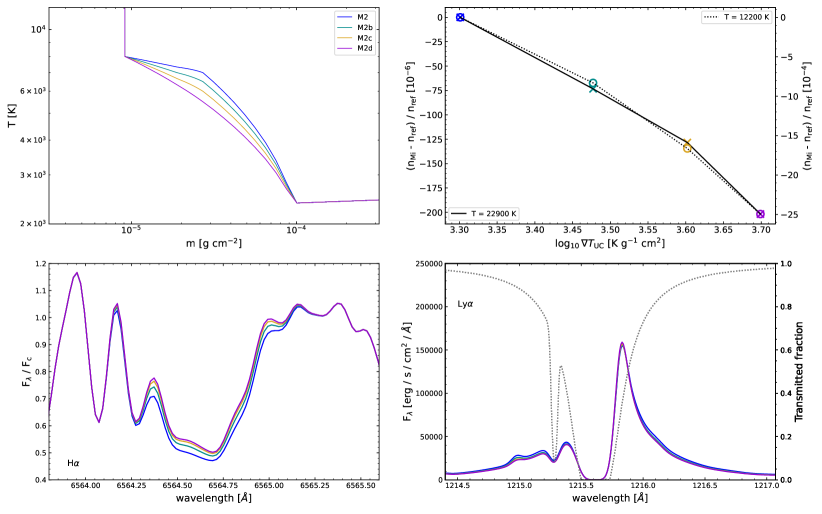
Figure 3: Top left: temperature structures of a series of models with varying temperature gradients in the upper chromosphere ($\nabla T_{\mathrm{UC}}$). Top right: changes in number densities of atomic hydrogen of models M2b to M2d ($n_{\mathrm{Mi}}$) relative to the reference model M2 (blue, $n_{\mathrm{ref}}$) at temperatures of 22 900 (solid line, left axis) and 12 200 K (dotted line, right axis) from where significant contributions to the Ly$\alpha$ and H$\alpha$ line flux arise, respectively (see Figure 1, left panel). They are plotted against the corresponding $\nabla T_{\mathrm{UC}}$ gradients. Colors coincide with the models depicted on the left-hand side. Circles depict variations in number density at 12 200 K and crosses those at 22 900 K. Increasing $\nabla T_{\mathrm{UC}}$ from M2 to M2d leads to a decrease in both $n_{\mathrm{Mi}}$ ($T=12\,200$ K) and $n_{\mathrm{Mi}}$ ($T=22\,900$ K), but the effect is significantly stronger for $n_{\mathrm{Mi}}$ ($T=12\,200$ K). Therefore, H$\alpha$ is more affected by this temperature profile parameter than Ly$\alpha$ (see also Figure B.1). Bottom: corresponding model spectra in the lines of Ly$\alpha$ (right, including the ISM transmission curve) and H$\alpha$ (left). This figure is continued in Figure B.2 in Appendix B for the C IV and He I IRT lines.

An important reason for the differences between models M1 and M2 shown in Figure 2 is the position of the transition region in terms of column mass densities as introduced in Section 2. The transition region is crucial for all of the lines considered in Figure 2. Increasing the present activity state, which corresponds to a transition region located at higher densities, i. e., model M2 compared to M1, strengthens the line absorption of the H$\alpha$ and He I IRT (Cram & Mullan, 1979; Avrett et al., 1994; Hintz et al., 2020). Yet the effects of changing the transition region densities are more obvious in the UV lines since they are formed at higher temperatures than H$\alpha$ and the He I IRT.

Figure 3 shows a series of models with similar temperature profiles but varying temperature gradients in the upper chromosphere (UC). Starting with model M2, we increased the temperature gradient of the upper chromosphere, as given by

$$\nabla T_{\mathrm{UC}}=\frac{\mathrm{d}T}{\mathrm{d}\log m},$$ (1)

where $T$ is the temperature and $m$ the column mass density. In this series, the upper chromosphere starts at $m=10^{-4.5}$ g cm^-2 and the corresponding temperatures vary in steps of 500 K from 5500 to 7000 K (from M2d to M2). The corresponding model spectra in the H$\alpha$ region illustrate a shift of the activity level (from M2d to M2; see also the activity measurements displayed in Figure B.1), i. e., it comes along with an enhancement in the H$\alpha$ line absorption (the H$\alpha$ equivalent width increases by 12.5 % from M2d to M2). The Ly$\alpha$ flux also increases, but the line is less affected than H$\alpha$ (the integrated Ly$\alpha$ flux changes by 4.6 % from M2d to M2). It has a similar effect on both hydrogen lines but is weaker than the shift of the transition region to higher densities (model M1 to M2, the integrated Ly$\alpha$ flux increases by 37.1 % while the H$\alpha$ equivalent width increases by 15.7 %). The resulting changes in the C IV and He I IRT lines when varying $\nabla T_{\mathrm{UC}}$ are illustrated in Figure B.2. Shifting the transition region to higher densities increases the strength of both hydrogen lines and also of the C IV line, while the He I IRT absorption deepens as seen in Figure 2. The C IV line behaves similarly but changes less when changing the temperature gradient in the upper chromosphere. The He I IRT absorption increases with a high-density transition region, but weakens when approaching a plateau-like structure in the temperature profile of the upper chromosphere. On the other hand, the Na I D₂ and bluest Ca II IRT lines mostly depend on the lower chromospheric temperature regions and are thus just marginally affected when adapting the upper chromospheric parameters.

The behavior of a line is dependent upon the number densities at the line formation depths, and thus these are useful for illustrating what happens when a prescribed atmospheric structure is modified. In Figure 3, we show the number densities of atomic hydrogen at two different locations in the transition region indicated by two different atmospheric temperatures. These are layers from which significant contributions to Ly$\alpha$ and H$\alpha$ originate. For this we used the temperatures of 22 900 and 12 200 K for Ly$\alpha$ and H$\alpha$, respectively. These temperatures correspond to the central temperatures from the formation regions indicated in Figure 1. An increase in the number density of atomic hydrogen where H$\alpha$ forms is connected with an increase in the H$\alpha$ absorption. The change in the number density of atomic hydrogen at 12 200 K from M2 to M2d is one order of magnitude larger than is the case in the temperature layer from which a significant contribution to Ly$\alpha$ arises. The number densities of atomic hydrogen at the Ly$\alpha$ and H$\alpha$ formation depths increase when shifting the transition region to higher densities as well as when establishing a plateau-like profile of the upper chromosphere ($\nabla T_{\mathrm{UC}}$ decreases from M2d to M2). However, a shift of the transition region to higher densities leads to an increase in the Ly$\alpha$ flux, but it does not necessarily lead to the formation of the H$\alpha$ line in the same way. These findings indicate that the line formation results from an interplay between several temperature profile properties, such as the temperature gradient of the upper chromosphere as well as the onset and temperature gradient of the transition region, rather than just shifting a prescribed temperature structure in terms of column mass densities.

These illustrations reveal that it is indeed quite difficult to reproduce the UV and VIS/NIR lines simultaneously with just one model. The UV lines arise from hotter layers in the transition region (Linsky, 2017) and are strongly dependent on its shape and also on the location of the temperature minimum (Peacock et al., 2019a), while the chromospheric densities are important for the lines in the VIS/NIR (Hintz et al., 2019), yet the location of the temperature minimum plays an important role in their formation as well. At this point it is necessary to account for requirements of the different line formation heights as well as for the discrepancies arising from the complexity of simultaneously modeling UV and VIS/NIR lines observed at different times. Observations from different time periods can be affected by the activity cycle and may require a different approach than modeling the considered lines with just one single model.

3.2 Linear combination of two models

By analyzing the line strengths of chromospheric indicators such as H$\alpha$ in M-dwarf stars it is possible to estimate surface filling factors of active regions (Giampapa, 1980, 1985). It is common to divide the surface into two components:

$$F=(1-A)\,F_{q}+A\,F_{a}$$ (2)

where $F$, $F_{q}$, and $F_{a}$ represent the total, quiet, and active line fluxes, respectively, and $A$ denotes the fraction of all active regions on the stellar surface while the fraction of quiet regions is given by the factor $(1-A)$. This filling-factor ansatz can be approximated by linear combinations of model components (Giampapa, 1985; Ayres et al., 2006). This method has already been used in the recent past using PHOENIX models by Hintz et al. (2019) following the ansatz of Eq. (2) in order to model active and variable M stars, including GJ 436. Hintz et al. (2019) found that the filling factor of the active model component increases with increasing activity states, but the difference in terms of the activity state between inactive and active model components decreases for less active stars.

Table 3: Estimating weighting factors ($w_{\mathrm{i}}$) in Eqs. (3) and (4) from line errors ($\sigma_{\mathrm{i}}$) and widths ($c_{\mathrm{i}}$).

Line	$\lambda_{\mathrm{i}}$ [$\AA$]	$c_{\mathrm{i}}$ [$\AA$]	$\sigma_{\mathrm{i}}$ [$\AA$]a	$w_{\mathrm{i}}$ [$\AA^{-2}$]
Ly${\alpha}$b	1215.7	3.5	2.01 E+4	2.47 E-10
C IV	1548.2	0.8	2.10 E+3	2.26 E-8
H${\alpha}$	6564.6	0.9	1.46 E-1	4.69 E+1
He I IRT	10 833.3	0.9	3.36 E-2	8.86 E+2

We linearly combine a model capable of reproducing the UV lines and another one that reproduces the VIS/NIR lines, aiming at an overall match of the investigated lines – models M1 and M2 from Figure 2, respectively. We use the Ly$\alpha$, C IV, H$\alpha$, and He I IRT lines for this purpose and we adapt the modified $\chi^{2}$-minimization used by Hintz et al. (2019) in order to look for the best combination of the two models. Due to the different line widths and strengths, we weight the respective line contributions when applying the modified $\chi^{2}$-minimization in the wavelength ranges of the lines in order to approach an equal treatment of the lines as follows:

$$\chi^{2}_{\mathrm{m}}=\sum_{\mathrm{i}}w_{\mathrm{i}}\,\chi^{2}_{\mathrm{i}},$$ (3)

where $\chi^{2}_{\mathrm{i}}$ corresponds to the sum of the quadratic model deviations from the observed flux values within a line $i$. The weighting factors $w_{\mathrm{i}}$ for the lines are determined from the standard deviations $\sigma_{\mathrm{i}}$ within the widths ($c_{\mathrm{i}}$) of the respective emission and absorption lines:

$$w_{\mathrm{i}}=1/\sigma_{\mathrm{i}}^{2}.$$ (4)

Table 3 lists the weighting factors, $c_{\mathrm{i}}$, and $\sigma_{\mathrm{i}}$ for the considered lines. With these modified $\chi^{2}$-values we are able to compare the linear combinations among the models and identify our best match. Applying these to the $\chi^{2}_{\mathrm{m}}$-minimization introduced above yields contributions of $(1-A)=80\,\%$ and $A=20\,\%$ from model M1 and model M2, respectively, to the linear combination. Including Na I D₂ and Ca II IRT lines in this procedure would only marginally affect the results since M1 and M2 look quite similar in these lines. The resulting best linear combination would be nearly identical to the one without Na I D₂ and Ca II IRT lines; the change in the fraction $A$ would be of the order of $\sim 1\%$. The red model spectrum in Figure 2 shows the corresponding modeled lines from the linear combination of these two models. It exhibits $\chi^{2}_{\mathrm{m}}=45.1$ compared to $\chi^{2}_{\mathrm{m}}=50.5$ for model M1 only, and $\chi^{2}_{\mathrm{m}}=134.4$ for M2, corresponding to an improvement of 10.7% from M1 and 66.4% from M2 for the overall match. With this approach we can get an overall match to the observations. This means that the H$\alpha$ and He I IRT cores are matched by the linear combination model while we obtain a reproduction of the Ly$\alpha$ and C IV lines as well.

The near-UV (NUV) HST observation of GJ 436 and the linear combination from Figure 2 are plotted in Figure 4. In general, the linear combination reproduces the observations in the range between $\sim$2000 and 2300 $\AA$ as well as in the Mg II h and k lines. We find model deviations from the NUV observation redwards of 2300 $\AA$, where there are some overpredicted Fe II features overlapping with V I, V II and Co II lines, for instance. Even though we did not aim at modeling the NUV region, we find that the synthetic spectrum from this model can also reproduce the NUV observation.

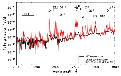
Figure 4: The linear combination obtained from Section 3.2 for the NUV region compared to an HST STIS observation (G230L grating) of GJ 436. The model spectrum is reduced to the resolving power of 1000 corresponding to the maximum resolution of the STIS G230L grating. Here we also indicate a couple of strong lines and line bands within this spectral region.

3.3 Discussion

In this paper, we have aimed at finding a model spectrum able to reproduce the average state of GJ 436. While we used the coadded template spectrum of GJ 436 observed with CARMENES over a time period from 2016 January to 2016 November to investigate its VIS/NIR spectral range, we used single HST observations from 2015 June to cover the UV region. The model study of Hintz et al. (2019) included an activity-related investigation on CARMENES observations of M dwarfs and revealed that GJ 436 is exhibiting low activity variations compared to four far more active stars in their sample – for instance, the observed H$\alpha$ and Ca II IRT lines of GJ 436 appeared in pure absorption and only showed marginal changes in their line strengths. The actual contrast in terms of activity between the two model components in the linear combination found here is relatively low, for example, compared to the combinations obtained for the four active stars investigated in Hintz et al. (2019). So the active component represents the active regions of an essentially not very active star, which is in agreement with the star’s measured $\log R^{\prime}_{\mathrm{HK}}<-5.1$ (e. g., Fuhrmeister et al., 2023). However, we cannot exclude stronger activity-related changes, although it has not been observed yet and GJ 436 only showed low activity in other studies (e. g., Lothringer et al., 2018).

For the Ly$\alpha$ line it is even harder to make a statement on the variability on GJ 436 because interstellar absorption considerably suppresses the observed line flux (e. g., Dring et al., 1997; Wood et al., 2005), and there is still a lack of continuous UV observations of M-dwarf stars. From the Sun it is known that Ly$\alpha$ is highly variable over a range of more than 30 % due to the stellar rotation and activity cycle (Vidal-Madjar, 1975). However, GJ 436 is known to be a bright Ly$\alpha$ emitter (Ehrenreich et al., 2011). Therefore, it was important to include the Ly$\alpha$ line in our modeling to take into account atmospheric heights where high-energy radiation is produced. To account for these difficulties we excluded the inner Ly$\alpha$ line core in our investigation and we also included a second strong line from the UV region. We also compared our final linear combination model spectrum to the observed NUV range of GJ 436 in order to verify that we obtained a model that also reproduces the spectral region between the UV and VIS/NIR lines discussed above.

As well as the astrophysical deficiencies described above there are also model-dependent issues as to why the observed lines are not entirely matched by the models. Model-related shortcomings may be the considered NLTE species set and the element abundances. One model with the chosen NLTE set incorporating most of the abundant elements already consumes several thousands of CPU hours. However, for future modeling purposes and with improving computing performances, it will become easier to take into account even more species in NLTE. Furthermore, future modeling should also test different element abundances. Trying to vary element abundances across the model atmosphere, which may be reasonable with respect to the very hot and low-density regime of the transition region, represents another possibility to improve the models. Besides, we use semiempirical temperature profiles to approach the nature of the chromosphere and lower transition region. Future modeling should test temperature structures that account for a balance between heat conduction, ambipolar diffusion, and radiative losses in order to establish a more realistic perspective on the low-density, atmospheric regions such as what has been done for solar models by Fontenla et al. (1990, 1991, 1993) using the PANDORA code (Avrett & Loeser, 1992), but with a comparably restricted NLTE set.

4 Summary and conclusion

In this work, we stated the difficulty of modeling planet-hosting star GJ 436 for different spectral features from the UV to the VIS/NIR wavelength regions. Different line formation temperatures that are separated by several thousand Kelvin and optically thick lines such as the hydrogen Ly$\alpha$ and H$\alpha$ lines that form over broad atmospheric regions reveal a high complexity when searching for a model able to match all considered spectral lines. The temperature structure itself plays a significant role for the final model spectrum when adjusting the structure parameters with regard to the different line responses. It is known that observed variabilities of active low-mass stars arise from starspots (Reinhold et al., 2019), thus it is generally reasonable to account for this by combining different models in order to approximate the real nature of the stellar surface. We applied a linear combination approach to simulate the heterogeneity of the stellar surface of GJ 436 and we were able to obtain an overall match of the UV and VIS/NIR lines. The more active model component in the combination better matches H$\alpha$ while the more inactive component better reproduces C IV. The higher activity state was necessary in order to reproduce the absorption strength of H$\alpha$. The preferred active model component contributes about 20 % to the linear combination, but the main difference between the two components is the transition region located at different densities. Because of the very different formation regions of the lines that are taken into account, we also checked the obtained combination in the intermediate range of the NUV. Therefore, we conclude that it is sufficient to model the M dwarf GJ 436 with a linear combination approach consisting of two model components. A similar approach should be considered to model other stars of this spectral type in the same way. Even though GJ 436 exhibits only small activity-related variations, we showed the efficiency of the linear combination of two model spectra, representing different activity states, for the reproduction of spectral features observed at different time periods. In general, this is a powerful and very flexible tool to match spectral features sensitive to stellar activity when regarding variable stars.

Appendix A Applying the Ly$\alpha$ ISM transmission curve

Supporting Figure 2, we depict in Figure A.1 how we apply the ISM transmission curve for GJ 436 using the results obtained from Youngblood et al. (2016) on model M2. Onto the original model M2 Ly$\alpha$ spectrum, we deploy the determined ISM transmission fractions in order to take into account the interstellar absorption in the line of sight before accounting for the instrumental broadening of the HST spectrograph. Thus, we can directly compare our modeled Ly$\alpha$ line to the observed one.

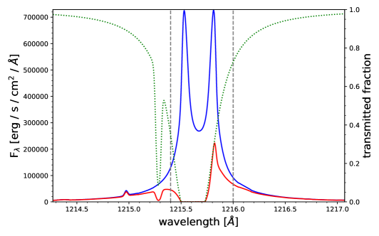
Figure A.1: Application of the Ly$\alpha$ ISM transmission curve (green dotted line) for GJ 436 as found by Youngblood et al. (2016) to our model M2 (blue solid line). The resulting modeled Ly$\alpha$ line is shown in red. We also indicate the Ly$\alpha$ line core area we neglected within our modified $\chi^{2}$-minimization by the two dashed vertical lines.

Appendix B Modeled line behavior when varying chromospheric temperature gradients

Figure B.1 shows the corresponding activity measurements for the Ly$\alpha$, C IV, H$\alpha$, and He I IRT lines as given by integrated line fluxes or equivalent widths for models M1 and M2 - M2d. Furthermore, as a supplement to Figure 3, we continue the displayed line behavior of the models in Figure B.2 for the lines of C IV and He I IRT as well as the Na I D₂, and bluest Ca II IRT lines when varying the temperature gradient ($\nabla T_{\mathrm{UC}}$) of the upper chromosphere.

Figure B.1: Activity measurements for model series M2 - M2d as given by the integrated line fluxes (LF, left panel) of Ly$\alpha$ (crosses) and C IV (pluses), as well as the equivalent widths (EW, right panel) of H$\alpha$ (circles) and the He I IRT (diamonds) for models M2 - M2d as a function of $\nabla T_{\mathrm{UC}}$. The colors of the models coincide with those in Figures 3 and B.2. We also show the corresponding values of M1 (green markers) except for the LF (C IV), which equals to 1251.1 erg s^-1 cm^-2.

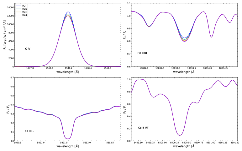
Figure B.2: Figure 3 continued for the C IV (upper left), He I IRT (upper right), Na I D₂ (lower right), and the bluest Ca II IRT (lower right) lines. The colors coincide with those used in Figure 3.

References

- Allart et al. (2018) Allart, R., Bourrier, V., Lovis, C., et al. 2018, Science, 362, 1384
- Alonso-Floriano et al. (2015) Alonso-Floriano, F. J., Morales, J. C., Caballero, J. A., et al. 2015, A&A, 577, A128
- Andretta & Giampapa (1995) Andretta, V., & Giampapa, M. S. 1995, ApJ, 439, 405
- Andretta & Jones (1997) Andretta, V., & Jones, H. P. 1997, ApJ, 489, 375
- Avrett et al. (1994) Avrett, E. H., Fontenla, J. M., & Loeser, R. 1994, in IAU Symposium, Vol. 154, Infrared Solar Physics, ed. D. M. Rabin, J. T. Jefferies, & C. Lindsey, 35
- Avrett & Loeser (1992) Avrett, E. H., & Loeser, R. 1992, Astronomical Society of the Pacific Conference Series, Vol. 26, The PANDORA Atmosphere Program (Invited Review), ed. M. S. Giampapa & J. A. Bookbinder, 489
- Ayres et al. (2006) Ayres, T. R., Plymate, C., & Keller, C. U. 2006, ApJS, 165, 618
- Barklem (2007) Barklem, P. S. 2007, A&A, 466, 327
- Bourrier et al. (2016) Bourrier, V., Lecavelier des Etangs, A., Ehrenreich, D., Tanaka, Y. A., & Vidotto, A. A. 2016, A&A, 591, A121
- Butler et al. (2004) Butler, R. P., Vogt, S. S., Marcy, G. W., et al. 2004, ApJ, 617, 580
- Cram & Mullan (1979) Cram, L. E., & Mullan, D. J. 1979, ApJ, 234, 579
- Díez Alonso et al. (2019) Díez Alonso, E., Caballero, J. A., Montes, D., et al. 2019, A&A, 621, A126
- Drawin (1968) Drawin, H.-W. 1968, Zeitschrift fur Physik, 211, 404
- Drawin (1969) Drawin, H. W. 1969, Zeitschrift fur Physik, 225, 470
- Dring et al. (1997) Dring, A. R., Linsky, J., Murthy, J., et al. 1997, ApJ, 488, 760
- Ehrenreich et al. (2011) Ehrenreich, D., Lecavelier Des Etangs, A., & Delfosse, X. 2011, A&A, 529, A80
- Ehrenreich et al. (2015) Ehrenreich, D., Bourrier, V., Wheatley, P. J., et al. 2015, Nature, 522, 459
- Falchi & Mauas (1998) Falchi, A., & Mauas, P. J. D. 1998, A&A, 336, 281
- Fontenla et al. (1990) Fontenla, J. M., Avrett, E. H., & Loeser, R. 1990, ApJ, 355, 700
- Fontenla et al. (1991) —. 1991, ApJ, 377, 712
- Fontenla et al. (1993) —. 1993, ApJ, 406, 319
- Fouqué et al. (2018) Fouqué, P., Moutou, C., Malo, L., et al. 2018, MNRAS, 475, 1960
- France et al. (2016) France, K., Loyd, R. O. P., Youngblood, A., et al. 2016, ApJ, 820, 89
- Fuhrmeister et al. (2005) Fuhrmeister, B., Schmitt, J. H. M. M., & Hauschildt, P. H. 2005, A&A, 439, 1137
- Fuhrmeister et al. (2006) Fuhrmeister, B., Short, C. I., & Hauschildt, P. H. 2006, A&A, 452, 1083
- Fuhrmeister et al. (2019) Fuhrmeister, B., Czesla, S., Hildebrandt, L., et al. 2019, A&A, 632, A24
- Fuhrmeister et al. (2023) Fuhrmeister, B., Czesla, S., Perdelwitz, V., et al. 2023, A&A, 670, A71
- Gaia Collaboration et al. (2021) Gaia Collaboration, Brown, A. G. A., Vallenari, A., et al. 2021, A&A, 649, A1
- Giampapa (1980) Giampapa, M. S. 1980, SAO Special Report, 389, 119
- Giampapa (1985) —. 1985, ApJ, 299, 781
- Gizis et al. (2002) Gizis, J. E., Reid, I. N., & Hawley, S. L. 2002, AJ, 123, 3356
- Gomes da Silva et al. (2011) Gomes da Silva, J., Santos, N. C., Bonfils, X., et al. 2011, A&A, 534, A30
- Hauschildt (1992) Hauschildt, P. H. 1992, J. Quant. Spec. Radiat. Transf., 47, 433
- Hauschildt (1993) —. 1993, J. Quant. Spec. Radiat. Transf., 50, 301
- Hauschildt & Baron (1999) Hauschildt, P. H., & Baron, E. 1999, Journal of Computational and Applied Mathematics, 109, 41
- Hintz et al. (2019) Hintz, D., Fuhrmeister, B., Czesla, S., et al. 2019, A&A, 623, A136
- Hintz et al. (2020) —. 2020, A&A, 638, A115
- Hubeny & Lites (1995) Hubeny, I., & Lites, B. W. 1995, ApJ, 455, 376
- Kulow et al. (2014) Kulow, J. R., France, K., Linsky, J., & Loyd, R. O. P. 2014, ApJ, 786, 132
- Kumar & Fares (2023) Kumar, M., & Fares, R. 2023, MNRAS, 518, 3147
- Kurucz & Bell (1995) Kurucz, R. L., & Bell, B. 1995, Atomic line list
- Lammer et al. (2007) Lammer, H., Lichtenegger, H. I. M., Kulikov, Y. N., et al. 2007, Astrobiology, 7, 185
- Landi et al. (2013) Landi, E., Young, P. R., Dere, K. P., Del Zanna, G., & Mason, H. E. 2013, ApJ, 763, 86
- Linsky (2017) Linsky, J. L. 2017, ARA&A, 55, 159
- Linsky et al. (2014) Linsky, J. L., Fontenla, J., & France, K. 2014, ApJ, 780, 61
- Lothringer et al. (2018) Lothringer, J. D., Benneke, B., Crossfield, I. J. M., et al. 2018, AJ, 155, 66
- Loyd et al. (2016) Loyd, R. O. P., France, K., Youngblood, A., et al. 2016, ApJ, 824, 102
- Loyd et al. (2023) Loyd, R. O. P., Schneider, P. C., Jackman, J. A. G., et al. 2023, AJ, 165, 146
- Magain (1986) Magain, P. 1986, A&A, 163, 135
- Marfil et al. (2021) Marfil, E., Tabernero, H. M., Montes, D., et al. 2021, A&A, 656, A162
- Martin et al. (2017) Martin, J., Fuhrmeister, B., Mittag, M., et al. 2017, A&A, 605, A113
- Martínez-Arnáiz et al. (2011) Martínez-Arnáiz, R., López-Santiago, J., Crespo-Chacón, I., & Montes, D. 2011, MNRAS, 414, 2629
- Nagel (2019) Nagel, E. 2019, PhD thesis, University of Hamburg
- Nortmann et al. (2018) Nortmann, L., Pallé, E., Salz, M., et al. 2018, Science, 362, 1388
- Peacock et al. (2019a) Peacock, S., Barman, T., Shkolnik, E. L., Hauschildt, P. H., & Baron, E. 2019a, ApJ, 871, 235
- Peacock et al. (2019b) Peacock, S., Barman, T., Shkolnik, E. L., et al. 2019b, ApJ, 886, 77
- Quirrenbach et al. (2018) Quirrenbach, A., Amado, P. J., Ribas, I., et al. 2018, in Society of Photo-Optical Instrumentation Engineers (SPIE) Conference Series, Vol. 10702, 107020W
- Reinhold et al. (2019) Reinhold, T., Bell, K. J., Kuszlewicz, J., Hekker, S., & Shapiro, A. I. 2019, A&A, 621, A21
- Robertson et al. (2016) Robertson, P., Bender, C., Mahadevan, S., Roy, A., & Ramsey, L. W. 2016, ApJ, 832, 112
- Rosenthal et al. (2021) Rosenthal, L. J., Fulton, B. J., Hirsch, L. A., et al. 2021, ApJS, 255, 8
- Salz et al. (2018) Salz, M., Czesla, S., Schneider, P. C., et al. 2018, A&A, 620, A97
- Spake et al. (2018) Spake, J. J., Sing, D. K., Evans, T. M., et al. 2018, Nature, 557, 68
- Stauffer & Hartmann (1986) Stauffer, J. R., & Hartmann, L. W. 1986, ApJS, 61, 531
- Suárez Mascareño et al. (2015) Suárez Mascareño, A., Rebolo, R., González Hernández, J. I., & Esposito, M. 2015, MNRAS, 452, 2745
- Tian et al. (2008) Tian, F., Kasting, J. F., Liu, H.-L., & Roble, R. G. 2008, Journal of Geophysical Research (Planets), 113, E05008
- Trainer et al. (2006) Trainer, M. G., Pavlov, A. A., Dewitt, H. L., et al. 2006, Proceedings of the National Academy of Science, 103, 18035
- Uitenbroek (2001) Uitenbroek, H. 2001, ApJ, 557, 389
- Vernazza et al. (1973) Vernazza, J. E., Avrett, E. H., & Loeser, R. 1973, ApJ, 184, 605
- Vernazza et al. (1981) —. 1981, ApJS, 45, 635
- Vidal-Madjar (1975) Vidal-Madjar, A. 1975, Sol. Phys., 40, 69
- Vidal-Madjar et al. (2004) Vidal-Madjar, A., Désert, J. M., Lecavelier des Etangs, A., et al. 2004, ApJ, 604, L69
- Wedemeyer et al. (2004) Wedemeyer, S., Freytag, B., Steffen, M., Ludwig, H.-G., & Holweger, H. 2004, A&A, 414, 1121
- Wood et al. (2005) Wood, B. E., Redfield, S., Linsky, J. L., Müller, H.-R., & Zank, G. P. 2005, ApJS, 159, 118
- Youngblood et al. (2016) Youngblood, A., France, K., Loyd, R. O. P., et al. 2016, ApJ, 824, 101
- Zechmeister et al. (2018) Zechmeister, M., Reiners, A., Amado, P. J., et al. 2018, A&A, 609, A12