Large-Scale Turbulent Pressure Fluctuations Revealed by Ned Kahn’s Artwork

Abstract

We investigate the dynamics of pendulum chains immersed in turbulent boundary layers. We combine laboratory experiments and video analysis of the kinetic facade exhibits by the artist Ned Kahn, composed of large-scale clusters of centimeter-sized plates oscillating freely in the wind. At the laboratory scale, we show that a one-dimensional pendulum chain immersed in a wind tunnel exhibits a wave dispersion relation derived from a Sine-Gordon equation. Under the wind action, the dynamical response is either dominated by a resonance phenomenon, or a linear response to pressure fluctuations. From amateur video analysis on large-scale kinetic facades, we show that the plate oscillation is driven by the same resonant response mechanisms and the apparent wavy pattern corresponds to the most energetic Fourier mode propagating at the advection speed of pressure fluctuations.

Introduction.— Ned Kahn is an American artist who constructs numerous exhibits inspired by the ephemera of nature. Amongst his works is the kinetic facade, a regular assembly of small aluminum plates covering entire facades of buildings in various countries (US, Scotland, Netherland, Switzerland). As the wind blows along the wall, the plates oscillate freely, creating wave-like large-scale patterns (Fig. 1a). The spatiotemporal structures could be revealed by the kinetic facades are the grail of any fluid mechanician, for whom measuring spatiotemporal structures of boundary layers in shear flows has been a long-standing challenge, and has mainly been investigated in numerical simulations of channel flows (Chung and Mckeon (2010); Jiménez (2018); Towne et al. (2020)) of increasing dimensions, from idealized to specific configurations for application to wind farms (Churchfield et al. (2012)). Spatiotemporal fluctuations of velocity at large scale He et al. (2017) are also key elements in wind farm design in order to minimize the global power fluctuations of a plant affected by long range fluctuations, and have been characterized by two point measurements in the far wake region Sørensen et al. (2002); Wetz et al. (2023); Vermeer et al. (2003). A direct visualisation of spatiotemporal pressure fluctuations in turbulent boundary layers is of great interest, and has been investigated experimentally ocassionally in laboratory experiments since the pioneering work of Dinkelacker Dinkelacker et al. (1977) who measured the spatiotemporal structures of pressure fluctuations using a Mylar^® plate and interference fringes. It has recently been shown that indirect insight can be obtained from the pattern imprints on a liquid surface below the onset of wind-wave generation on an air-water interface; these imprints are also the signature of turbulent pressure fluctuations Perrard et al. (2019). However, to the best of our knowledge, the origin of the kinetic-facade motion has not been investigated. It could be the result of numerous phenomena, such as fluid-structure instabilities observed in flapping wings Shelley and Zhang (2011) or canopies De Langre (2008), or bistability of pendulums in turbulent flows Gayout et al. (2021).

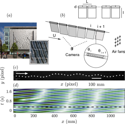
Figure 1: (a) Example of Ned Kahn’s kinetic facade exhibits with wave-like patterns ((Kahn, 2014)). (b) Sketch of the experimental set-up, composed of a thin plate chain elastically coupled, and placed in the measuring section of the wind tunnel. (c) Snapshot of the oscillation of pendulums, highlighted with white circles for visibility. (d) Spatiotemporal chart of the pendulum oscillation after image processing, with the instant illustrated above (black dashed line).

Experimental set-up.— To investigate the origin of these dynamical patterns, we designed a one-dimensional experimental model at the laboratory scale, composed of a chain of elastically coupled pendulums, as sketched in fig. 1b. The chain consists of $36$ 3D-printed plates of height $l=48.5$ mm, plate distance $L=32.5$ mm, and width $28.5$ mm, for a total chain length of $1.1$ m . The plates are connected by a nylon fishing wire to control the coupling constant between adjacent elements. The i-th pendulum of inclination angle $\theta_{i}$ then interacts with its neighbors ($i-1$) and ($i+1$) with a coupling force linearly proportional to the angle difference. In the absence of wind, the motion of each pendulum follows the one-dimensional discrete Sine-Gordon equation:

$$\partial_{tt}\theta_{i}-L^{2}\omega_{w}^{2}\Delta\theta_{i}+\lambda\partial_{t}\theta_{i}+\omega_{0}^{2}\sin\theta_{i}=0$$ (1)

where $\Delta\theta_{i}=(\theta_{i+1}-2\theta_{i}+\theta_{i-1})/L^{2}$ is the discrete second spatial derivative of $\theta$ on site $i$, $\lambda$ is the damping coefficient, and $\omega_{0}=\sqrt{g/\ell}$ is the natural angular frequency with $g$ the acceleration of gravity and $\ell=2/3l$ is the effective pendulum length of a thin plate. The velocity $L\omega_{w}$ originates from the pendulum coupling through the wire elastic torsion, with $\omega_{w}$ the wire elastic torsion frequency. From elastica, we have $\omega_{w}=\sqrt{GJ_{w}/(LI_{p})}$ with $G$ the wire shear modulus, $J_{w}=\pi a^{4}/32$ the polar second moment of area of the wire and $I_{p}=ml^{2}/3$ the moment of inertia of the pendulum with respect to $x$ axis. In the presence of an air flow, a torque-induced angular acceleration $A_{i}=T_{i}/I_{p}$ applied to each pendulum appears as a source term on the right-hand-side of eq. 1.

The chain is placed at the symmetry plane of an open circuit suction wind tunnel with a free-stream wind speed $U$ ranging from 0 to $8$ m/s. Fishing wire of two different diameters $a=0.2$ and $0.8$ mm was used to vary the coupling between plates. The pendulum dynamics are recorded from below, and a white spot on each pendulum is used to track the instantaneous oscillation angles. For each wind speed, $90000$ images are recorded at a frame rate of $300.03$ Hz. From the sets of images, a spot-recognition code with sub-pixel accuracy is used to extract the pendulum angles $\theta_{i}(t)$. Fig. 1c,d show respectively a snapshot of the pendulum chain, and the spatiotemporal diagram of the inclination angles $\theta_{i}(t)$.

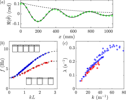
Figure 2: (a) Spatial structure of the mode $\Re(\tilde{\theta}(x,f))$ at $f=3.63$ Hz. A fit by $\theta_{0}\cos(kx+\phi)\exp(-\Lambda x)$ is superimposed (black solid line) as well as the exponential decay envelope (dashed line).(b) Dispersion relation for the chain of pendulums in the absence of wind, with a wire diameter $a=0.8$ mm and a distance between plates $L=32.5$ mm (blue circle) and $L=65$ mm (red square). The black dashed lines correspond to Eq. 2 with $f_{0}=2.77$ Hz. (c) Temporal damping coefficient $\lambda$ as a function of the wavenumber $k$.

To validate the Sine-Gordon model, we first perform a set of experiments without wind. The first pendulum element is mechanically excited with a motorized hammer with a beat frequency ranging from $1.3-6.5$ Hz. We record all $\theta_{i}$ as a function of time, and filtered the signals at frequencies ranging from $f_{0}$ to 9 Hz to extract the complex mode $\tilde{\theta}(x,f)$. We extract the wavenumber $k$ and the spatial damping factor $\Lambda$ using a fit of the form $\theta_{0}\cos(kx+\phi)\exp(-\Lambda x)$. Figure 2a shows the dispersion relation at rest, for 36 plates (blue) and 18 plates (red) separated by $2L$. In both cases, we recover the expected minimum cut-off frequency $f_{min}=f_{0}=2.77$ Hz, and the maximum cut-off frequency $f_{max}$ near $kL=\pi$ reduces from $9.5$ Hz to $7$ Hz as the spacing is doubled. The dispersion relation

$$\omega_{r}^{2}=\omega_{0}^{2}+4\omega_{w}(a)^{2}\sin^{2}\left(\frac{kL}{2}\right),$$ (2)

of eq. 1 is superimposed (black dashed line) without any fitting parameter, and shows excellent quantitative agreement with the experimental data. Using the group velocity $c_{g}=\rm{d}\omega/\rm{d}k$, we converted the spatial damping coefficient $\Lambda$ into a temporal damping coefficient $\lambda=\Lambda c_{g}$, shown in figure 2b as a function of the wavenumber $k$. The data for the standard chain (blue) and the spaced out chain (red) collapse onto a single master curve, showing that the coupling between adjacent pendulum plays a negligible role in the dissipation of pendulum motions. The upper frequency cutoff is also influenced by the wire diameter. For a weaker elastic coupling ($a=0.2$ mm, not shown), the maximum cutoff reduces drastically from $9.5$ Hz to $2.83$ Hz: the dispersion relation becomes almost independent of the wave number.

We now blow wind over the pendulum chain. As above, we measure each $\theta_{i}$ as a function of time, and we compute the Fourier transform $\hat{\theta}_{k,f}$ of $\theta$ both in $x$ and time. The colormaps of $\hat{\theta}_{k,f}$ at the wind speed of $U=2.6$ m/s are shown in figure 3 for a wire diameter $a=0.8$ mm (a) and $a=0.2$ m (b). In both cases, the prominent feature is the strong energy localization along two main branches. A first branch is found surrounding $f=kU_{c}/2\pi$, where $U_{c}$ is a characteristic velocity extracted from a linear fit of amplitude maxima (solid red line). A second branch surrounding the red dashed line is the wave dispersion relation slightly upshifted from the rest case. We then introduce an additional term in the dispersion relation (eq. 3):

$$\omega_{r}^{2}=\omega_{0}^{2}+4\left(\omega_{w}^{2}+\frac{u_{s}^{2}}{L^{2}}\right)\sin^{2}\left(\frac{kL}{2}\right),$$ (3)

where the factor $4u_{s}^{2}/L^{2}$ is associated to the wind-induced modification of the dispersion relation, assuming a linear dependence of this extra term on the pendulums’ local curvature, we have $u_{s}^{2}\sim\Delta\theta$. This phenomenological wind-induced coupling velocity $u_{s}$ is shown as a function of wind speed (inset figure 3b). The coupling velocity $u_{s}$ is a small fraction of $U_{c}$. With the new dispersion relation, we find an excellent agreement between eq. 3 and the experimental data, with $\omega_{0}$ and $\omega_{w}$ set fixed to their values at rest.

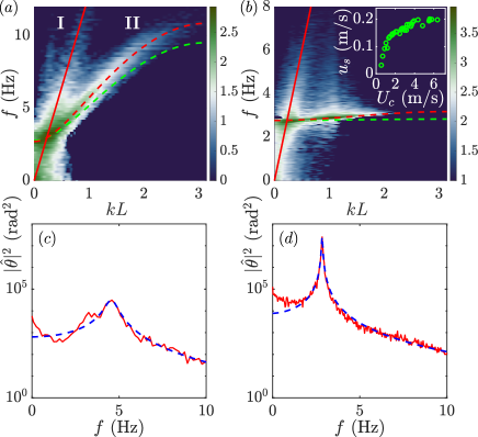
Figure 3: (a, b) spatiotemporal spectrum of pendulum oscillations $|\hat{\theta}|_{f,k}$ (a: $a=0.2$ mm; b: $a=0.8$ mm), with the dispersion relation at rest (green dashed line) from eq. 2, the modified one from eq. 3 (red dashed line) and the best fit of constant advection speed $f\propto kL$ (solid red line). Inset: evolution of wind-induced coupling velocity $u_{s}$ as a function of the convection velocity $U_{c}$. (c, d) Temporal spectrum $|\hat{\theta}|^{2}$ at $kL=0.72$ (red line) and the fit around the resonant frequency $f_{r}$ (blue dashed line).

Resonant response in Fourier space.— The accumulation of energy surrounding two branches, one being the wave dispersion relation, and one being the maximum energy of the forcing recalls the spatiotemporal resonance mechanism introduced by Phillips Phillips (1957) and others Perrard et al. (2019); Nové-Josserand et al. (2020) in the context of wind-generated water waves by pressure fluctuations. Assuming a statistically stationary state, eq. 1 can be transformed into Fourier space to express the Fourier transform $\theta(k,\omega)$ as:

$$|\hat{\theta}|^{2}=\frac{|\hat{\mathcal{A}}|^{2}}{(\omega^{2}-\omega_{r}^{2}(k))^{2}+\lambda^{2}(k)\omega^{2}},$$ (4)

where the denominator is a convolution kernel, and $\hat{\mathcal{A}}$ is the Fourier transform of the torques-induced acceleration applied to each pendulum by the turbulent fluctuations. The maximum response in Fourier space is therefore either located where the forcing $\hat{\mathcal{A}}$ is maximum (branch I) or along the dispersion relation ($\omega\sim\omega_{r}$) (branch II). At a given wavenumber and an angular frequency $\omega\sim\omega_{r}(k)$, the pendulum chain resonates with the spectral modes of $\hat{\mathcal{A}}$, the growth being limited by dissipative effects. To test the validity of eq. 4, we compute the energy spectrum $|\hat{\theta}|^{2}$ as a function of $f$, as shown for $kL=0.72$ in fig. 3 (red line) for a wire diameter $a=0.8$ mm (c) and $a=0.2$ mm respectively (d). We fit the source term $\hat{\mathcal{A}}$ by $\hat{\mathcal{A}}=\hat{\mathcal{A}}_{r}+\gamma(\omega-\omega_{r})$ with two adjustable parameters $\hat{\mathcal{A}}_{r}$ and $\gamma$, corresponding to a first-order Taylor expansion of $\hat{\mathcal{A}}$ in the vicinity of the resonant frequency $\omega_{r}$. We find a quantitative agreement between eq. 4 (blue dashed line) and the experimental measurements.

The branch (I) is located away from the resonant curve and corresponds to a direct response to wind-induces acceleration, and the slope $2\pi f_{I}/k_{I}$ is the advection speed at the scale $k_{I}$ Wills (1964); Del Alamo and Jiménez (2009); Moin (2009). We determine the convection velocity by measuring the wavenumber giving the maximum amplitude at each frequency (Hussain and Clark (1981); Goldschmidt et al. (1981)), away from the resonant branch ($f_{c}<f_{0}$). These structures correspond to the signature of pressure fluctuations integrated over each plate, advected at a constant speed independent of their size (see red solid lines in Fig. 3a,b).

The pendulum chain response is then the superposition of the large-scale imprints of turbulent fluctuations along $\omega=U_{c}k$, and the resonant response near $\omega=\omega_{r}(k)$. For vanishing mechanical coupling, the angular frequency $\omega_{r}$ becomes almost independent of $k$. The advection speed of the large-scale structures can thus be approximated by $2\pi f_{0}/k_{max}$, where $k_{max}$ is the wavenumber of the most energetic Fourier mode, located at the intersection of the two branches. Using our experiment of observations, we have developed a theoretical framework that we will now use to analyze the recordings of the kinetic facades.

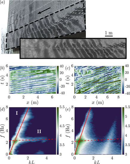
Figure 4: (a) Snapshot of wave patterns on Ned Kahn’s facade with the region of interest delimited by dashed lines and the corrected image. (b,c) spatiotemporal charts of the image pixel intensity for an image row parallel to the wind flow. (d,e) spatiotemporal spectrum of the image pixel intensity, averaged over the image rows parallel to the wind flow.

Survey data collection.— Let now examine the 2D dynamics of Ned Kahn’s large-scale kinetic facades using amateurs’ online videos. We gathered data on YouTube.com and Vimeo.com, with frame rate ranging from $25$ to $29$ Hz, and we investigate on the exhibits’ dimensions from various sources. Most facades are covered with square plates of flapping length size from $51$ mm to $127$ mm, and separated by a distance ranging from $1.2$ to $1.6$ times the pendulum length. To account for the variability in viewing angles, we apply a quadratic transformation that maps the quadrilateral distorted plate images to rectangles. The spatial scale is recovered from the plate dimensions and their known spacing distances. A video snapshot and a corrected image of the Swiss Science Center Technorama (Kahn, 2002) are shown in fig. 4a. Eventually, A total of 18 videos taken on 6 different facades are studied.

We perform a spatiotemporal FFT on the corrected images. Fig. 4 shows two typical examples from two facades (left: Glacial Facade (Kahn, 2006), right: Digitized Field (Kahn, 2005)). The spatiotemporal diagrams of the image intensity along a line parallel to the direction of the wave propagation are shown in Fig. 4b,c and the corresponding spectra in Fourier space, averaged over the direction perpendicular to the wave propagation (d,e). Similar to our laboratory results, the fluctuation intensity peaks around two branches, which we consider to be the wave dispersion relation (branch II) and the convection velocity of large scale structures (branch I). In Ned Kahn’s facades, since plates are free to swing with no elastic coupling between them, the slight inclination of the dispersion relation is assumed to be wind-driven, as observed for small wire diameters. The similarity between spectral maps of fluctuations and our laboratory experiments can then be used to deduce the traveling speed of turbulent fluctuations on the kinetic facades.

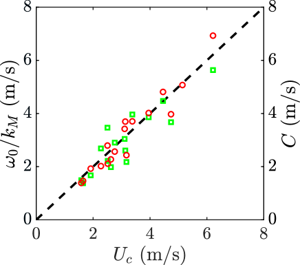
Figure 5: Compilation of the measured convection velocities from two techniques, as a function of the advection speed $U_{c}$ extracted from a fit on the turbulent branch (fig. 4)d). Red circle: direct measurements of the phase speed $C$ of the dominant wave by tracking of one typical crest. green squares: $f_{0}$ and $k_{M}$ separately deduced from temporal and spatial Fourier transform on the image sequence.

For each sequence, we measured the convection velocity $U_{c}$ from a linear fit of the branch I of the spatio-temporal spectrum. As the dispersion relation does not significantly depend on the wavenumber $k$, this convection speed can be obtained from a single image analysis. Indeed, assuming that the frequency of maximum response $f_{M}$ corresponds to the natural oscillation frequency $f_{0}$ of the pendulum, we estimate the convection velocity as $\omega_{0}/k_{M}$, where the wavenumber $k_{M}$ is measured from the wavelength of the dominant patterns of the Ned Kahn’s facade. Fig. 5 shows the estimated convection velocity $\omega_{0}/k_{M}$ (blue square) as a function of the convection velocity $U_{c}$ obtained from spectral analysis. We eventually compared to a third measurement technique. From a series of image, we measured the traveling speed $C$ of the dominant wave crest, as shown in fig 5 (red circle). We found a quantitative agreement between the two alternative methods, which do not require prior determination of the spatiotemporal spectrum, and the advection speed $U_{c}$.

The relation in Fourier space between the pendulum angles and the turbulent forcing thus provides an original, cost-effective and promising pathway to characterize spatio-temporal turbulent fluctuations at large scales, in particular for atmospheric turbulent boundary layers.

We acknowledge fruitful discussions with Ned Kahn, Antonin Eddi, Laurette Tuckerman, Marc Rabaud, Frédéric Moisy, Aliénor Rivière and Philippe Bourianne. We are specially grateful to Amaury Fourgeaud for technical support, Gauthier Bertrand for the wind tunnel design and Marc Fermigier for scientific support. We also acknowledge Jörg Moor from Swiss Science Center Technorama and John Gray from Dundee City Council for providing Ned Kahn’s facade dimensions. This work was supported by a PSL Junior Fellow Starting Grant 2022.

References

- Chung and Mckeon (2010) D. Chung and B. J. Mckeon, Journal of Fluid Mechanics 661, 341 (2010).
- Jiménez (2018) J. Jiménez, Journal of Fluid Mechanics 842, P1 (2018).
- Towne et al. (2020) A. Towne, A. Lozano-Durán, and X. Yang, Journal of Fluid Mechanics 883, A17 (2020).
- Churchfield et al. (2012) M. J. Churchfield, S. Lee, J. Michalakes, and P. J. Moriarty, Journal of turbulence , N14 (2012).
- He et al. (2017) G. He, G. Jin, and Y. Yang, Annu. Rev. Fluid Mech. 49 (2017).
- Sørensen et al. (2002) P. Sørensen, A. D. Hansen, and P. A. C. Rosas, Journal of wind engineering and industrial aerodynamics 90, 1381 (2002).
- Wetz et al. (2023) T. Wetz, J. Zink, J. Bange, and N. Wildmann, Boundary-Layer Meteorology 187, 673 (2023).
- Vermeer et al. (2003) L. Vermeer, J. N. Sørensen, and A. Crespo, Progress in aerospace sciences 39, 467 (2003).
- Dinkelacker et al. (1977) A. Dinkelacker, M. Hessel, G. E. A. Meier, and G. Schewe, Phys. of Fluids 20 (1977).
- Perrard et al. (2019) S. Perrard, A. Lozano-Durán, M. Rabaud, M. Benzaquen, and F. Moisy, Journal of Fluid Mechanics 873, 1020 (2019).
- Shelley and Zhang (2011) M. J. Shelley and J. Zhang, Annual Review of Fluid Mechanics 43, 449 (2011).
- De Langre (2008) E. De Langre, Annu. Rev. Fluid Mech. 40, 141 (2008).
- Gayout et al. (2021) A. Gayout, M. Bourgoin, and N. Plihon, Phys. Rev. Lett. 126 (2021).
- Kahn (2014) N. Kahn, “Project lions,” https://nedkahn.com/portfolio/project-lions/ (2014).
- Phillips (1957) O. M. Phillips, Journal of fluid mechanics 2, 417 (1957).
- Nové-Josserand et al. (2020) C. Nové-Josserand, S. Perrard, A. Lozano-Durán, M. Benzaquen, M. Rabaud, and F. Moisy, Physical Review Fluids 5, 124801 (2020).
- Wills (1964) J. Wills, Journal of Fluid Mechanics 20, 417 (1964).
- Del Alamo and Jiménez (2009) J. C. Del Alamo and J. Jiménez, Journal of Fluid Mechanics 640, 5 (2009).
- Moin (2009) P. Moin, Journal of fluid mechanics 640, 1 (2009).
- Hussain and Clark (1981) A. Hussain and A. Clark, AIAA journal 19, 51 (1981).
- Goldschmidt et al. (1981) V. Goldschmidt, M. Young, and E. Ott, Journal of Fluid Mechanics 105, 327 (1981).
- Kahn (2002) N. Kahn, “Technorama facade,” https://nedkahn.com/portfolio/technorama-facade/ (2002).
- Kahn (2006) N. Kahn, “Glacial facade,” https://nedkahn.com/portfolio/glacial-facade/ (2006).
- Kahn (2005) N. Kahn, “Digitized field,” https://nedkahn.com/portfolio/digitized-field/ (2005).