Phase Transitions of Diversity in Stochastic Block Model Dynamics

Abstract

This paper proposes a stochastic block model with dynamics where the population grows using preferential attachment. Nodes with higher weighted degree are more likely to recruit new nodes, and nodes always recruit nodes from their own community. This model can capture how communities grow or shrink based on their collaborations with other nodes in the network, where an edge represents a collaboration on a project.

Focusing on the case of two communities, we derive a deterministic approximation to the dynamics and characterize the phase transitions for diversity, i.e. the parameter regimes in which either one of the communities dies out or the two communities reach parity over time.

In particular, we find that the minority may vanish when the probability of cross-community edges is low, even when cross-community projects are more valuable than projects with collaborators from the same community.

1 Introduction

Academic institutions and large technology companies have been increasing their focus on hiring diverse faculty members and employees, particularly at senior levels  [BGLW18, SDG22]. Multiple papers in the broader computer science community have addressed issues around fair hiring or selection processes (e.g. [SDG22, KMR16, MPB⁺21, SHL21]). This paper considers what happens after hiring. We focus on the recruitment of candidates and growth of minority communities within organizations over time, in the context of the collaboration networks in the organization.

An important part of recruitment and retention is the climate of an organization, which is heavily influenced by the interpersonal network of the members. Such networks and social capital [Bou18] have a tremendous impact of the success of an individual [Put00].  [LACL19] shows how collaborations with top scientists can have significant impacts on the careers of junior scientists. Additionally, network ties are known to have impact on employment [CAI05], career-advancement [Tha97, CPT23], and educational outcomes [CAPZ09, KRT⁺23].

The structures of both personal and professional networks are strongly influenced by the homophily principle, which states that a person is more likely to form connections with individuals that have shared characteristics [MSLC01, SMSL14]. Homophily can contribute to occupation-based segregation (i.e., individuals of the same gender/ethnicity seem to cluster into similar jobs) as well as establishment-based segregation (i.e. individuals of similar ethnicity/gender work at the same institutions), which in turn can contribute to wage gaps [PM95]. Thus, people are more likely to recruit members of their own communities to their organizations. Meanwhile, individuals are more likely to join organizations where those similar to themselves have been successful; for example, newly recruited women often ask other women about their experiences in an organization. The work in [GUSA05] has shown that recruitment processes can affect network structure. In this paper, we consider how the network structure can affect recruitment.

We consider a stochastic block model [HLL83] with two communities, red and blue. Edges in the graph represent collaborations on projects between agents, and the weight associated with the edge represents the value or impact of the project. Multiple new nodes join the network at every time step. To capture homophily, nodes recruit other nodes of the same color (red/blue). The population grows using preferential attachment [BA99, BJN⁺02], where the attachment is based on the weighted degrees of the nodes. Thus, the more successful a community is—as measured by the weight of its projects—the more new nodes from that community join the graph.

1.1 Related work

Network formation.

We are motivated to model scientific collaboration networks, the growth of which has been studied in [BJN⁺02, HZLG08]. Others have examined how identity (e.g. gender) plays a role in this collaboration network [AMK⁺16, Ger22].

Different strategic aspects of collaboration networks have been considered; in particular, [JW03] considers a model where agents prefer to collaborate with nodes that have few edges (i.e. other collaborations), since this may indicate they have more available time to work on a joint project.

In contrast, [CAPZ09] considers a social network model where edges in the network have weights, and the payoff to an agent is a function not only of their own effort but also of the effort of their peers (i.e. those they are connected to in the network). Our model also considers weighted edges, and the payoff to an agent is the sum of the weights across all its edges at a particular time, but we do not consider strategic aspects. [KRT⁺23] addresses the problem of circumventing in-group bias that may appear in collaborations among university students on course projects.

The classical Barabasi-Albert algorithm for generating random scale-free networks using preferential attachment was introduced in [BA99]. [SHC20] considered a model of biased networks related to ours, where each node belongs to a community (e.g. red or blue). Nodes form connections according to the following principles:

  

Community affiliation: When a node enters the network, it chooses label red with a probability $r$, and blue with probability $1-r$;

  

Rich-get-richer: Each arriving node chooses to connect to some other node according to preferential attachment (i.e. with probability proportional to that node’s degree);

  

Homophily: If the two nodes from the previous step have the same label, an edge is formed; otherwise, the new node accepts the connection with probability $p$, where $0<p<1$, and the process is repeated until an edge is formed.

In this setting, [SHC20] considered the problem of seeding: how to introduce early adopters (e.g. nodes from under-represented communities) in the network so that fairer outcomes are achieved in the long term. Moreover, [SHC20] prove the existence of an analytical condition in which diversity acts as a catalyst for efficiency and analyze experimentally scientific networks using DBLP data.

The seeding or influence maximization problem was posed in [DR01]. An algorithmic formulation and analysis was given in [KKT03], which identified a class of naturally occurring processes where the influence maximization problem reduces to maximizing a submodular function under a cardinality constraint. Due to the desirable properties of submodular functions, this connection leads to efficient approximation algorithms for influence maximization. Learning to influence from observations of cascades was studied in [BIS17]. For an extensive survey on network formation and its connections to games and markets, see the book [KE12].

Stochastic block models.

The stochastic block model is a generative model for random graphs introduced in [HLL83], where there is a set $[n]=\{1,\ldots,n\}$ of nodes, each belonging to a community $C_{1},\ldots,C_{k}$, and a $k\times k$ symmetric probability matrix $\mathbf{p}$. A random graph is generated as follows: for each pair of vertices $u\in C_{i}$ and $v\in C_{j}$, generate the edge $(u,v)$ with probability $p_{i,j}$. A classic question is community recovery: given one or more graphs generated in this fashion, recover the underlying communities of the nodes. Weighted stochastic block models were formulated in [AJC13, AJC14, Pei18]. A survey on stochastic block models can be found in [Abb17].

Our model is informed by works such as [XH14, LEN18] that consider time-evolving stochastic block models, with a fixed set of nodes. Our model explicitly considers the addition of new nodes at each time step, and these new nodes join using preferential attachment, similar to [CCL13].

Biases in algorithmic decision making.

Studies have investigated how automated decision-making can have positive feedback effects of reinforcing biases over time [LM88, BS16, LWH⁺20, EFN⁺18]. Our model shows that without high-value cross-community collaborations, there can be a feedback effect where the majority community grows while the minority community decays. [LDR⁺18] observed that common static fairness criteria can worsen long-term well-being. To show this, [LDR⁺18] considered a one-step feedback model to analyze how (classification) decisions change the underlying population over time.

Urn models.

Our model is also strongly related to the Polya urn model, which first appeared in [EP23, Pol31] and features an urn containing red and blue balls. The urn evolves in discrete time steps. At each step, a ball is drawn uniformly at random, its color is observed, and then it is returned to the urn together with a new ball of the same color. Questions of interest include the ratio of red to blue in the long term and the stochastic path leading to it. A generalization is where the urn has balls of $k$ colors. Whenever a ball of color $i$ is drawn, $A_{i,j}$ balls of color $j$ are brought to the urn, for each $j\in\{1,\ldots,k\}$, where $\mathbf{A}=\{A_{i,j}\}_{i,j\in[k]}$ is the “schema”. A book on the Polya urns with schemas can be found in [Mah08].

Another generalization of the Polya urn was analyzed in [HLS80], where there is an urn with some initial number of red and blue balls. In each iteration, if the fraction of red balls is $x$, then with probability $f(x)$ a red ball is added next and with probability $1-f(x)$ a blue ball is added , where $f:[0,1]\to[0,1]$ is a function. Another generalization, where the update function can be time-dependent, was analyzed in [Pem90]. Nonlinear Polya urn processes with fitness were studied in  [JFRT16]. Our model can be seen as an urn which is time dependent (since the probability of a red ball being added depends both on the fraction of red and the total number of balls, which is equivalent to time dependence), but where multiple balls are added at each point in time.

The Polya urn model illustrates the rich get richer phenomenon, also known as the “Matthew effect” or “cumulative advantage”. [Pem07] surveys urn models together with their analysis techniques and applications, such as growth of social or neural networks, dynamics in games and markets [Pem07]. A probabilistic model for the early phase of neuron growth was proposed in [KK01], where growing neurites compete with each other and longer ones have more chances to grow.

Evolution of populations.

The evolution of populations has been studied under forces such as genetic drift, selection, mutation, and migration [Now06]. Some of these processes can be seen as urn models, where the composition of different types of marbles (gene variants) in a jar changes over time. In the Wright-Fisher process, there is an initial generation with some pool of genes. Then new generations appear such that each copy of a gene found in the new generation is drawn independently at random from the copies of the gene in the old generation; the generations do not overlap. In the Moran process [Mor58], the generations are overlapping. The self-organization of matter from the lens of evolving macro-molecules was studied in [Eig71]. For an overview of evolutionary game dynamics, see [HS03]. The convergence, mixing time, and computational questions arising in the evolution of populations have also been studied (see, e.g., [DSV12, PSV16]).

Inequality in games and markets.

At the level of countries, a global trend of escalating economic inequality has been reported  [Nat]. Extensive discussion and modeling of this phenomenon can be found in [Art94, PG15]. To counter the mounting accumulation of wealth that seems intrinsically tied to capitalist economies, [Pik14] proposed strategies like substantial wealth and inheritance taxes. Mathematical analyses showing the emergence of inequality in games and markets include [BMN18] and [GKM⁺19]. In non-atomic congestion games, [GKM⁺19] showed that introducing an optimal mechanism may settle or even exacerbate social inequality.

In networked production economies where players use proportional response dynamics to update their strategies, [BMN18] showed that players get differentiated over time into two classes: the “rich” (who participate in the most efficient production cycle) and the “poor” (who do not); moreover, the inequality gaps between the rich and the poor players grow unboundedly over time. In our model, biases of the different nodes (players) may cause a similar rich-get-richer phenomenon, even when diverse teams have better performance.

1.2 Main contributions

This paper introduces a stochastic model for network growth in Sec. 2 that captures how network ties can influence community growth in the network. The model has two main parameters: the probability of forming an edge (collaboration), captured by the probability matrix $\mathbf{p}$; and the value/weight of an edge, captured by the weight matrix $\boldsymbol{\zeta}$. Both the probability of forming an edge and its value depend on the communities of its endpoints.

We derive (Sec. 3, 4) and analyze (Sec. 5) a deterministic approximation of the stochastic model and show that it closely mirrors the behavior of the stochastic model. We find that the deterministic model with two communities has three fixed points, at $x=0,1/2,1$, where $x$ is the fraction of red in the system.

We identify a key ratio, $\rho$, which depends on $\mathbf{p}$ and $\boldsymbol{\zeta}$. When $\rho>1$, only $0$ and $1$ are stable fixed points, which means that one of the communities will necessarily vanish. This is possible if the probability of cross-edges is low, even if cross-community projects are more valuable than monochrome projects (i.e. projects with collaborators from the same community). The situation is reversed when $\rho<1$.

Main Theorem (informal): Consider the stochastic block model dynamics with two communities of Definition 2. The dynamic starts with a given graph and proceeds to refresh its edges while new nodes arrive through preferential attachment based on weighted degree in each round.

The resulting dynamical system admits a deterministic approximation, which unfolds as a function of the minority’s fraction. For the deterministic approximation system we have:

1. The fixed points of the system are at $0$, $1/2$, and $1$.

2. There exists a parameter, $\rho$, dependent on the probability and weight matrix of the underlying stochastic block model, which determines the behavior of the system:

   • If $\rho>1$, the minority vanishes in the limit, with the fixed points at $0$ and $1$ being stable and the fixed point at $1/2$ unstable.

   • If $\rho=1$, the minority fraction remains constant throughout time.

   • If $\rho<1$, the minority eventually achieves parity, with the fixed point at $1/2$ being stable and the fixed points at $0$ and $1$ unstable.

2 Model

We define the base model, which generates a random graph through a weighted stochastic block model. Then we describe the growth dynamics, where new nodes arrive while the edges are refreshed.

2.1 Weighted Stochastic Block Model

We consider the following random graph generation process. Each node has a color, red or blue.

Definition 1 (Stochastic Block Model).

Let $[n]=\{1,\ldots,n\}$ be a set of nodes, so that each node $i$ has color $c_{i}\in\{R,B\}$, where $R=1$ is red and $B=2$ is blue. Let $\mathbf{p}=\begin{bmatrix}{a}&{b}\\ {b}&{a}\end{bmatrix}$ and $\boldsymbol{\zeta}=\begin{bmatrix}\alpha&\beta\\ \beta&\alpha\end{bmatrix}$ where $a,b,\alpha,\beta\in\mathbb{R}_{+}\,.$

Generate a weighted random graph on $[n]$, so that for each pair of nodes $i,j\in[n]$ the weight of edge $(i,j)$ is:

• With probability ${p_{c_{i},c_{j}}}/{n}$, let $w_{i,j}:=\zeta_{c_{i},c_{j}}$.

• With remaining probability, let $w_{i,j}:=0$.

We refer to $\mathbf{p}$ as the probability matrix and $\boldsymbol{\zeta}$ as the weight matrix. The matrix $\mathbf{p}$ dictates edge existence, while the weights of edges that exist are dictated by $\boldsymbol{\zeta}$. In general formulations of the weighted stochastic block model, the weight of an edge is drawn from a distribution that depends on the communities of the endpoints. We focus on the special case where this distribution is supported at a single point.

Interpretation of the model. We illustrate the stochastic block model through a scenario of agents working on projects in an organization:

There is a set of agents $[n]=\{1,\ldots,n\}$ that belong to one of two communities, red or blue. Node $i$ has community $c_{i}\in\{R,B\}$.

Edges between agents indicate collaborations on projects. Agents may collaborate in pairs, or work individually on projects. Each pair of agents $(i,j)$ can collaborate on at most one project. Self loops are allowed: edge $(i,i)$ means agent $i$ works alone on a project.

The probability that agents $i$ and $j$ collaborate on a joint project is $p_{c_{i},c_{j}}/n$. Thus the probability of a project between agents $i$ and $j$ depends on the communities of $i$ and $j$, and the total number of agents.

If agents $i$ and $j$ collaborate on a project, i.e. form edge $(i,j)$, then the weight of the resulting project is $\zeta_{c_{i},c_{j}}$. The weight can indicate the value/impact of the project and depends only on the communities of agents $i$ and $j$.

An agent’s success is determined by the collective weight of all of their projects, both collaborative and individual.

The dependence on the total number of nodes in the probability $p_{c_{i},c_{j}}/n$ of generating edge $(i,j)$ ensures the expected total number of projects that an agent works on remains bounded even as the size of the graph grows.

2.2 Stochastic Block Model Dynamics

We first motivate our model for the stochastic block dynamics, then give the mathematical definition.

Motivation. The dynamics capture the connection between recruitment/hiring, and the existing climate, collaborations and related success in the organization through the following features:

Hiring/recruitment happens at discrete time intervals (e.g. every year for an academic institution). Collaborative projects are refreshed on a similar time scale (e.g. every year). Thus, at every time step, edge connections between nodes are refreshed.

Red agents recruit other red agents, and blue agents recruit other blue agents.

The higher the weight of an agent the more likely they are to recruit a new agent from their community. This captures two things: more successful agents are more likely to recruit other agents (e.g. by giving more frequent talks where they advertise their organization); and agents are more likely to join organizations where agents from their community are happy and successful.

New nodes arrive arrive by preferential attachment. Red nodes arrive at a rate that is proportional to the total weight of projects in the red community at that time; and similarly for blue agents.

Note the number of red nodes recruited at a time does not depend only on the existing number of red nodes, but on the total weight of their projects (i.e. their weighted degree).

Let $w_{u}=\sum_{v\in V}w_{u,v}$ denote the weighted degree of vertex $u\in V$ and $W=\sum_{u\in V}w_{u}$ the sum of weighted degrees of all nodes. Sampling a vertex with likelihood given by their weighted degree means that vertex $u\in V$ is selected with probability ${w_{u}}/{W}$.

Next we define the stochastic block dynamics, which generates a sequence of graphs $\{G_{t}\}_{t=1}^{\infty}$. Given $G_{t-1}$, an intermediate random graph $G_{t-1}^{+}$ is obtained by refreshing the edges of $G_{t-1}$, where an edge is refreshed by drawing it again according to the stochastic block model with probability matrix $\mathbf{p}$ and weight matrix $\zeta$. Then, we grow $G_{t-1}^{+}$ by having a number $(m_{t})$ of nodes join using preferential attachment to obtain $G_{t}$.

Definition 2 (Stochastic Block Model Dynamics).

Let ${V}_{0}=\{1,\ldots,n_{0}\}$ be an initial set of vertices, each red or blue. At every time unit $t=1,2,\ldots$, the next steps take place:

1. Generate an intermediate graph $G_{t-1}^{+}$ on vertices ${V}_{t-1}^{+}:={V}_{t-1}$ from the stochastic block model with probability matrix $\mathbf{p}$ and weight matrix $\boldsymbol{\zeta}$ (e.g. the agents in ${V}_{t-1}$ start pairwise/solo projects).

2. Initialize ${G}_{t}={G}_{t-1}^{+}$. Independently sample with replacement $m_{t}$ vertices $v_{1},\ldots,v_{m_{t}}\in{V}_{t-1}^{+}$, each with likelihood given by their weighted degree. Each sample $v_{i}$ brings in a new vertex $u_{i}$ with the same color and they form an edge. Vertex $u_{i}$ and edge $(v_{i},u_{i})$ are added to ${G}_{t}$ (e.g., agent $v_{i}$ recruits $u_{i}$).

Constant fraction of arriving nodes: We focus on the scenario where the number of nodes arriving is a constant fraction $\lambda\in(0,1)$ of the existing population. That is, the random variable $m_{t}$ for the number of arriving nodes is $m_{t}\in\{\lfloor\lambda\cdot n_{t-1}\rfloor,\lceil\lambda\cdot n_{t-1}\rceil\}$ such that $\operatorname{\mathbb{E}}[m_{t}]=\lambda\cdot n_{t-1}$, where $n_{t-1}$ is the number of nodes in ${G}_{t-1}$. $\square$

Constant fraction of arriving nodes models the early phases of a growing organization. Generally speaking, other regimes for $m_{t}$ could also be of interest.

W.l.o.g., red is the initial minority, so $n_{0}^{R}\leq n_{0}^{B}$.

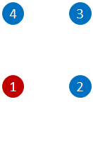
(a) Set $V_{0}$.

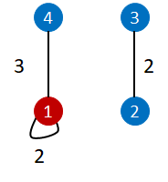
(b) Graph $G_{0}^{+}$.

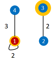
(c) Graph $G_{0}^{+}$; samples $1,3,3$.

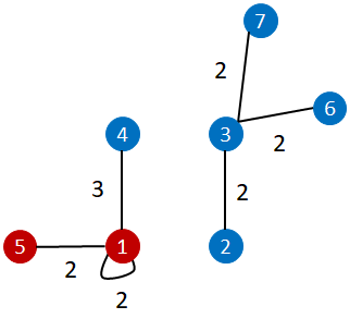
(d) Graph ${G}_{1}$. Each sample brings in a new node of the same color and they form an edge. That is, $1$ brings $5$, the first occurrence of $3$ brings $6$, and the second occurrence of $3$ brings $7$.

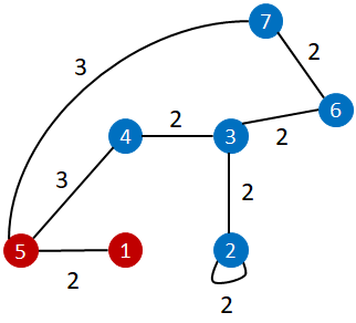
(e) Graph $G_{1}^{+}$. New edges are drawn between the vertices of $G_{1}$ to generate $G_{1}^{+}$.

Figure 1: Initial steps of the stochastic block model dynamics from Definition 2 illustrated. Suppose $\mathbf{p}=[[0.75,0.25],[0.25,0.75]]$, the weights are $\boldsymbol{\zeta}=[[2,3],[3,2]]$, and $\lambda=3/4$. Figure (a) shows the initial set of nodes $V_{0}=\{1,2,3,4\}$. Figure (b) shows a realization of the random graph $G_{0}^{+}$ generated using the stochastic block model on $V_{0}$ with the parameters. Figure (c) shows the samples $(1,3,3)$ drawn from the vertices of $G_{0}^{+}$ according to the weighted degree distribution of $G_{0}^{+}$. Figure (d) shows how each sample $v_{i}$ brings in a new node $u_{i}$, which copies $v_{i}$’s color and they form an edge. The graph obtained is $G_{1}$. Figure (e) shows graph $G_{1}^{+}$, generated using the same parameters on the vertices of $G_{1}$.

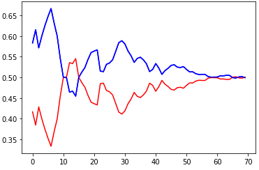
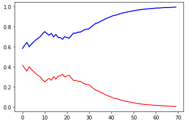
Figure 2: Trial runs of the stochastic block dynamics from Definition 2 with $11$ initial nodes. Red is the initial minority, starting with $5$ nodes in both cases. The $X$ axis shows time and the $Y$ axis shows the value of the fraction of red nodes. In (a) the fraction of red nodes reaches 50% in the limit, while in (b) it goes to zero in the limit. The probability matrix is $\mathbf{p}=[[0.75,0.25],[0.25,0.75]]$ in both cases (a) and (b). The fraction of nodes arriving in each round is $\lambda=0.1$. The weight matrix is $\boldsymbol{\zeta}=[[1,100],[100,1]]$ in (a) and $\boldsymbol{\zeta}=[[100,1],[1,100]]$ in (b).

Figure 1 illustrates the initial steps of the dynamic for a small number of initial nodes. A picture with trial runs of the dynamic that shows the fraction of red nodes over time is included in Figure 2.

3 Deterministic Approximation

In this section we deduce a deterministic approximation for the random system of Definition 2 and prove that it closely mirrors the stochastic model when the fraction of red (i.e. the minority fraction) is not arbitrarily close to zero.

We first introduce some notation that will be useful. In the sequence of graphs from Definition 2, we index the vertices $1,2,\ldots$. Thus if at some point the existing vertices are $\{1,\ldots,k\}$, then the next arriving node is denoted $k+1$.

In the setting of Definition 2, for each time step $t\in\mathbb{N}$:

• Let $\mathcal{F}_{t}$ be the history at the end of round $t$ for the process $\{G_{t}\}_{t=0}^{\infty}$.

• Let $\phi_{t}=\frac{n_{t}^{R}}{n_{t}}$ be the fraction of red nodes in ${G}_{t}$.

• Let $w_{i,j}^{+}(t-1)$ be the weight of edge $(i,j)$ in the graph $G_{t-1}^{+}$. Let $R_{t}$ be the weight of color red and $B_{t}$ the weight of color blue, respectively, in graph $G_{t-1}^{+}$. That is,

  $$R_{t} =\sum_{i\in[n_{t-1}]:c_{i}=R}\;\;\sum_{j\in[n_{t-1}]}w_{c_{i},c_{j}}^{+}(t-1)\,.$$ (1)

  $$B_{t} =\sum_{i\in[n_{t-1}]:c_{i}=B}\;\;\sum_{j\in[n_{t-1}]}w_{c_{i},c_{j}}^{+}(t-1)\,.$$ (2)

• Let $m_{t}^{R}$ and $m_{t}^{B}=m_{t}-m_{t}^{R}$ be the number of red and blue nodes, respectively, arriving at time step $t$.

Next we prove there exists a function $\Gamma:[0,1]\to[0,1]$ such that if $\phi_{t-1}$ (i.e. the fraction of the minority at time $t-1$) is above $1/\sqrt{n_{t-1}}$ and the initial number ($n_{0}$) of nodes is large enough, then

$$\bigl{(}1-o(1)\bigr{)}\left(\frac{\phi_{t-1}+\lambda\cdot\Gamma(\phi_{t-1})}{1+\lambda}\right)\leq\operatorname{\mathbb{E}}[\phi_{t}\mid\mathcal{F}_{t-1}]\leq\bigl{(}1+o(1)\bigr{)}\left(\frac{\phi_{t-1}+\lambda\cdot\Gamma(\phi_{t-1})}{1+\lambda}\right),$$

where

$$\Gamma(x) =\frac{{a\alpha}\cdot x^{2}+{b\beta}\cdot x\cdot(1-x)}{{a\alpha}\cdot x^{2}+2{b\beta}\cdot x\cdot(1-x)+{a\alpha}\cdot(1-x)^{2}}\,.$$ (3)

This will allow us to conclude that the dynamical system evolves approximately as follows:

$$\operatorname{\mathbb{E}}[\phi_{t}\mid\mathcal{F}_{t-1}]\approx\frac{\phi_{t-1}+\lambda\cdot\Gamma(\phi_{t-1})}{1+\lambda}\,.$$ (4)

Lemma 1.

Suppose there is a constant $\epsilon\in(0,1/2)$ so that

$$\left(\frac{1}{n_{t-1}}\right)^{\frac{1}{2}-\epsilon}\leq\phi_{t-1}\leq\frac{1}{2}\,.$$ (5)

Then there exists a constant $C=C(\epsilon,a,\alpha,b,\beta)$ so that when $n_{0}\geq C$,

$$\mathcal{L}(n_{t-1})\leq\operatorname{\mathbb{E}}[\phi_{t}\mid\mathcal{F}_{t-1}]\leq\mathcal{U}(n_{t-1}),$$

where $\mathcal{L},\mathcal{U}:\mathbb{N}\to\mathbb{R}$ are defined by

$$\mathcal{U}(n) =\frac{\phi_{t-1}+\frac{\lceil\lambda\cdot n\rceil}{n}\cdot\left(1+{1}/{n^{\epsilon/5}}\right)\cdot\Gamma(\phi_{t-1})}{1+\frac{\lfloor\lambda n\rfloor}{n}}\mbox{ and }\;\mathcal{L}(n)=\frac{\phi_{t-1}+\frac{\lfloor\lambda\cdot n\rfloor}{n}\cdot\left(1-{1}/{n^{\epsilon/5}}\right)\cdot\Gamma(\phi_{t-1})}{1+\frac{\lceil\lambda n\rceil}{n}}\,.$$ (6)

Proof.

For a fixed round $t$, each arriving node has the same probability of being red. The probability that one arriving node is red equals $R_{t}/(R_{t}+B_{t})$. Taking expectation, since the number of arriving nodes is $m_{t}\in\{\lfloor\lambda\cdot n_{t-1}\rfloor,\lceil\lambda\cdot n_{t-1}\rceil\}$, we have

$$\sum_{i=1}^{\lfloor\lambda\cdot n_{t-1}\rfloor}\operatorname{\mathbb{E}}\left[\frac{R_{t}}{R_{t}+B_{t}}\mid\mathcal{F}_{t-1}\right] \leq\operatorname{\mathbb{E}}\left[m_{t}^{R}\mid\mathcal{F}_{t-1}\right]\leq\sum_{i=1}^{\lceil\lambda\cdot n_{t-1}\rceil}\operatorname{\mathbb{E}}\left[\frac{R_{t}}{R_{t}+B_{t}}\mid\mathcal{F}_{t-1}\right]\,.$$ (7)

By Lemma 2, we have

$$\left(1-{1}/{n_{t-1}^{\epsilon/5}}\right)\cdot\frac{\operatorname{\mathbb{E}}[R_{t}\mid\mathcal{F}_{t-1}]}{\operatorname{\mathbb{E}}[{R_{t}}+{B_{t}}\mid\mathcal{F}_{t-1}]}\leq\operatorname{\mathbb{E}}\left[\frac{R_{t}}{R_{t}+B_{t}}\mid\mathcal{F}_{t-1}\right]\leq\left(1+{1}/{n_{t-1}^{\epsilon/5}}\right)\cdot\frac{\operatorname{\mathbb{E}}[R_{t}\mid\mathcal{F}_{t-1}]}{\operatorname{\mathbb{E}}[{R_{t}}+{B_{t}}\mid\mathcal{F}_{t-1}]}\,.$$ (8)

Combining (7) and (8), we obtain that under (5),

$$\lfloor\lambda\cdot n_{t-1}\rfloor\left(1-{1}/{n_{t-1}^{\epsilon/5}}\right)\frac{\operatorname{\mathbb{E}}[R_{t}\mid\mathcal{F}_{t-1}]}{\operatorname{\mathbb{E}}[{R_{t}}+{B_{t}}\mid\mathcal{F}_{t-1}]} \leq\operatorname{\mathbb{E}}\left[m_{t}^{R}\mid\mathcal{F}_{t-1}\right]$$

$$\leq\lceil\lambda\cdot n_{t-1}\rceil\left(1+{1}/{n_{t-1}^{\epsilon/5}}\right)\frac{\operatorname{\mathbb{E}}[R_{t}\mid\mathcal{F}_{t-1}]}{\operatorname{\mathbb{E}}[{R_{t}}+{B_{t}}\mid\mathcal{F}_{t-1}]}\,.$$ (9)

Since the graphs $G_{t-1}^{+}$ and $G_{t-1}$ have the same vertices, we have

$$\operatorname{\mathbb{E}}[{R_{t}}\mid\mathcal{F}_{t-1}]=\left(n_{t-1}^{R}\right)^{2}\cdot\frac{a\alpha}{n_{t-1}}+n_{t-1}^{R}n_{t-1}^{B}\cdot\frac{b\beta}{n_{t-1}}\;;$$

$$\operatorname{\mathbb{E}}[{B_{t}}\mid\mathcal{F}_{t-1}]=\left(n_{t-1}^{B}\right)^{2}\cdot\frac{a\alpha}{n_{t-1}}+n_{t-1}^{R}n_{t-1}^{B}\cdot\frac{b\beta}{n_{t-1}}\,.$$ (10)

Combining the identities in (10) gives

$$\frac{\operatorname{\mathbb{E}}[R_{t}\mid\mathcal{F}_{t-1}]}{\operatorname{\mathbb{E}}[R_{t}+B_{t}\mid\mathcal{F}_{t-1}]} =\frac{{a\alpha}\left(n_{t-1}^{R}\right)^{2}+{b\beta}\left(n_{t-1}^{R}\cdot n_{t-1}^{B}\right)}{{a\alpha}\left(n_{t-1}^{R}\right)^{2}+2{b\beta}\left(n_{t-1}^{R}\cdot n_{t-1}^{B}\right)+{a\alpha}\left(n_{t-1}^{B}\right)^{2}}$$

$$=\frac{{a\alpha}\left(\phi_{t-1}\right)^{2}+{b\beta}\phi_{t-1}(1-\phi_{t-1})}{{a\alpha}\left(\phi_{t-1}\right)^{2}+2{b\beta}\phi_{t-1}(1-\phi_{t-1})+{a\alpha}(1-\phi_{t-1})^{2}}$$

$$=\Gamma(\phi_{t-1})\,.$$ (11)

The number of red nodes in $\mathcal{G}_{t}$ is $n_{t}^{R}=n_{t-1}^{R}+m_{t}^{R}$, so $\phi_{t}=\frac{n_{t-1}^{R}+m_{t}^{R}}{n_{t}}$. By definition of the dynamic,

$$n_{t}\in\Bigl{\{}n_{t-1}+\lfloor\lambda n_{t-1}\rfloor,n_{t-1}+\lceil\lambda n_{t-1}\rceil\Bigr{\}}\mbox{ with }\operatorname{\mathbb{E}}[n_{t}\mid\mathcal{F}_{t-1}]=(1+\lambda)n_{t-1}\,.$$ (12)

Using (9), (11), and (12), we can upper bound the expected fraction of red at time $t$ when (5) holds:

$$\operatorname{\mathbb{E}}[\phi_{t}\mid\mathcal{F}_{t-1}] \leq\frac{n_{t-1}^{R}+\operatorname{\mathbb{E}}[m_{t}^{R}\mid\mathcal{F}_{t-1}]}{n_{t-1}+\lfloor\lambda n_{t-1}\rfloor}=\frac{\phi_{t-1}+\frac{\lceil\lambda\cdot n_{t-1}\rceil}{n_{t-1}}\cdot\left(1+{1}/{n_{t-1}^{\epsilon/5}}\right)\cdot\Gamma(\phi_{t-1})}{1+\frac{\lfloor\lambda n_{t-1}\rfloor}{n_{t-1}}}\,.$$ (13)

Similarly, we can lower bound the expected fraction of red at time $t$ as follows when (5) holds:

$$\operatorname{\mathbb{E}}[\phi_{t}\mid\mathcal{F}_{t-1}] \geq\frac{n_{t-1}^{R}+\operatorname{\mathbb{E}}[m_{t}^{R}\mid\mathcal{F}_{t-1}]}{n_{t-1}+\lceil\lambda n_{t-1}\rceil}=\frac{\phi_{t-1}+\frac{\lfloor\lambda\cdot n_{t-1}\rfloor}{n_{t-1}}\cdot\left(1-{1}/{n_{t-1}^{\epsilon/5}}\right)\cdot\Gamma(\phi_{t-1})}{1+\frac{\lceil\lambda n_{t-1}\rceil}{n_{t-1}}}\,.$$ (14)

Combining (13), (14), (6), we obtain $\mathcal{L}(n_{t-1})\leq\operatorname{\mathbb{E}}[\phi_{t}\mid\mathcal{F}_{t-1}]\leq\mathcal{U}(n_{t-1})\,.$ This completes the proof of the lemma. ∎

The proof of the next lemma is deferred to the appendix.

Lemma 2.

In the setting of Lemma 1,

$$\left(1-\frac{1}{n_{t-1}^{\epsilon/4}}\right)\frac{\operatorname{\mathbb{E}}[{R_{t}}]}{\operatorname{\mathbb{E}}[{R_{t}}+{B_{t}}]}<\frac{{R_{t}}}{{R_{t}}+{B_{t}}}<\left(1+\frac{1}{n_{t-1}^{\epsilon/4}}\right)\frac{\operatorname{\mathbb{E}}[{R_{t}}]}{\operatorname{\mathbb{E}}[{R_{t}}+{B_{t}}]}\,.$$

with probability at least $1-\frac{8}{e^{C_{1}\cdot n_{t-1}^{\epsilon}}}$, where $C_{1}=\min\left\{{a}/{12},{b}/{6}\right\}\,.$ Moreover,

$$\left(1-\frac{1}{n_{t-1}^{\epsilon/5}}\right)\frac{\operatorname{\mathbb{E}}[{R_{t}}]}{\operatorname{\mathbb{E}}[{R_{t}}+{B_{t}}]}<\operatorname{\mathbb{E}}\left[\frac{{R_{t}}}{{R_{t}}+{B_{t}}}\right]<\left(1+\frac{1}{n_{t-1}^{\epsilon/5}}\right)\frac{\operatorname{\mathbb{E}}[{R_{t}}]}{\operatorname{\mathbb{E}}[{R_{t}}+{B_{t}}]}\,.$$

By Lemma 1, when the fraction of the minority, $\phi_{t-1}$, is strictly above $1/\sqrt{n_{t-1}}$, we have

$$\mathcal{L}(n_{t-1})\leq\operatorname{\mathbb{E}}[\phi_{t}\mid\mathcal{F}_{t-1}]\leq\mathcal{U}(n_{t-1}).$$

Moreover,

$$\lim_{n\to\infty}\mathcal{L}(n)=\lim_{n\to\infty}\mathcal{U}(n)=\frac{\phi_{t-1}+\lambda\cdot\Gamma(\phi_{t-1})}{1+\lambda}\,.$$ (15)

4 Deterministic System

The approximation in (4), which in the limit is given by the right hand side of (15), motivates us to introduce the following deterministic system to approximate the behavior of the stochastic system for large number of nodes.

Definition 3 (Deterministic System).

Let $\Phi_{0}\in(0,1/2]$. Define the sequence $\{\Phi_{t}\}_{t=0}^{\infty}$ such that

$$\Phi_{t}=\frac{\Phi_{t-1}+\lambda\cdot\Gamma(\Phi_{t-1})}{1+\lambda},$$ (16)

recalling that $\Gamma(x)$

$$\Gamma(x)=\frac{{a\alpha}\cdot x^{2}+{b\beta}\cdot x\cdot(1-x)}{{a\alpha}\cdot x^{2}+2{b\beta}\cdot x\cdot(1-x)+{a\alpha}\cdot(1-x)^{2}}\,.$$

Figures 3 and 4 show a trajectory of the deterministic system of Definition 3 together with the trajectory of the stochastic system of Definition 2 started from the same initial configuration.

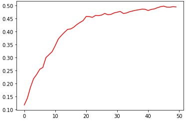
(a) Random system

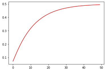
(b) Deterministic system

Figure 3: Figure (a) shows the random system with $n=70$ initial nodes such that $n_{R}=5$ are red. The probability matrix is $\mathbf{p}=\begin{bmatrix}{0.75}&{0.25}\\ {0.25}&{0.75}\end{bmatrix}$ and the weight matrix is $\mathbf{\omega}=\begin{bmatrix}1&100\\ 100&1\end{bmatrix}$. We have $\rho\approx 0.03$. The fraction of nodes arriving in each round is $\lambda=0.1$. Figure (b) shows the corresponding deterministic system, for the same initial parameters, as $n\to\infty$.

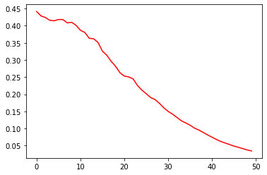
(a) Random system

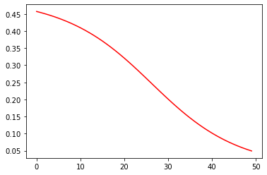
(b) Deterministic system

Figure 4: Figure (a) shows the random system with $n=70$ initial nodes such that $n_{R}=32$ are red. The probability matrix is $\mathbf{p}=\begin{bmatrix}{0.95}&{0.05}\\ {0.05}&{0.95}\end{bmatrix}$ and the weight matrix is $\mathbf{\omega}=\begin{bmatrix}1&1.2\\ 1.2&1\end{bmatrix}$. We have $\rho\approx 15.8$. The fraction of nodes arriving in each round is $\lambda=0.1$. Figure (b) shows the corresponding deterministic system, for the same initial parameters, as $n\to\infty$.

The deterministic model can be thought of as a version of the stochastic system where each node is an infinitesimal particle (e.g. of some fluid such as water), which is partially red and partially blue instead of a discrete node with one color.

Recall that at each time step in the stochastic system, every arriving node $u$ becomes red with some probability $p$ and blue with probability $1-p$. The deterministic system captures a similar dynamic, but each arriving node $u$ is an infinitesimal particle which has a mix of two colors: red in proportion of $p$ and blue in proportion of $1-p$. At each point in time, if there are currently $x$ units of fluid, then $\lambda x$ units are added in the next iteration. Explicit node edges are no longer considered in the deterministic approximation, but instead we have the product of the amount of red fluid and the amount of blue fluid to correspond to the product of red-blue edges.

The variable of interest will be the evolution of the ratio red/blue over time.

5 Analysis of the Deterministic System

Next, we understand how the ratio of red to blue evolves over time in the deterministic system, by identifying the fixed points of the model, and their stability properties. In Lemma 3 first compute a simplified update function for the system of Definition 3, which shows that the key parameters are the fraction of red at each point in time and the constant ratio $\rho:={a\alpha}/{(b\beta)}$.

Proposition 1 shows that if $\rho>1$ then the fraction of the minority (red) can die out regardless of the initial state.

Lemma 3.

The dynamical system in Definition 3 has update function, i.e. $f:[0,1]\to[0,1]$ such that $\Phi_{t+1}=f(\Phi_{t})$ given by:

$$f(x)=\frac{2x^{3}(\rho-1)-x^{2}(\rho-1)(2-\lambda)+x(\rho+\lambda)}{(1+\lambda)\Bigl{(}2x^{2}(\rho-1)-2x(\rho-1)+\rho\Bigr{)}},\;\;\mbox{ where }\rho:=a\alpha/(b\beta)\,.$$

Proof.

By Definition 3, we have $\Phi_{t+1}=\frac{\Phi_{t}+c\cdot\Gamma(\Phi_{t})}{1+\lambda},$ where $\Gamma(x)$ is as in (3).

Consider the function $f:[0,1]\to[0,1]$ given by $f(x)=\bigl{(}{x+\lambda\cdot\Gamma(x)}\bigr{)}/\bigl{(}{1+\lambda}\bigr{)}$. Substituting $\Gamma(x)$ in the expression for $f(x)$ and re-arranging the terms gives

$$f(x) =\frac{x+\lambda\cdot\left(\frac{a\alpha\cdot x^{2}+b\beta\cdot x\bigl{(}1-x\bigr{)}}{a\alpha\cdot x^{2}+2b\beta\cdot x\bigl{(}1-x\bigr{)}+a\alpha\cdot\bigl{(}1-x\bigr{)}^{2}}\right)}{1+\lambda}$$

$$=\frac{2x^{3}(\rho-1)-x^{2}(\rho-1)(2-\lambda)+x(\rho+\lambda)}{(1+\lambda)\left(2x^{2}(\rho-1)-2x(\rho-1)+\rho\right)}$$

where the equality is obtained by dividing by $b\beta$, substituting $\rho=a\alpha/(b\beta)$ and simplifying. ∎

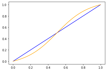
(a) The yellow line shows the function $f$ with $\rho=12$ and $\lambda=2$. The blue line shows the identity function. The fixed points $0$ and $1$ of $f$ are stable while $1/2$ is unstable.

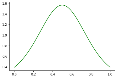
(b) The derivative $f^{\prime}$ when $\rho=12$ and $\lambda=2$.

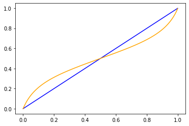
(c) The function $f$ when $\rho=0.2$ and $\lambda=2$. The blue line shows the identity function. The fixed points $0$ and $1$ of $f$ are unstable while $1/2$ is stable.

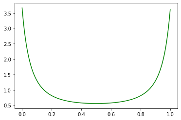
(d) The derivative $f^{\prime}$ when $\rho=0.2$ and $\lambda=2$.

Figure 5: The function $f$ and its derivative $f^{\prime}$ for two values of $\rho$. In both cases $\lambda=2$. Note here we are choosing a $\lambda>1$ to better illustrate the curvature of the function, but the shape remains similar for all $\lambda>0$.

Next, we identify the fixed points of the system.

Lemma 4.

Consider the update function $f$ for the deterministic system. If $\rho\neq 1$ then the set of fixed points of $f$ is $\left\{0,\frac{1}{2},1\right\}$. If $\rho=1$ then $f(x)=x$ for all $x\in[0,1]$.

Proof.

To find the fixed points, we require that $f(x)=x$. Equivalently,

$$f(x)=x\iff$$

$$2x^{3}(\rho-1)-x^{2}(\rho-1)(2-\lambda)+x(\rho+\lambda)=(1+\lambda)\left(2x^{3}(\rho-1)-2x^{2}(\rho-1)+\rho x\right)\iff$$

$$\lambda(\rho-1)x\bigl{(}2x-1\bigr{)}\bigl{(}x-1\bigr{)}=0\,.$$

By definition, $\lambda>0$. If $\rho=1$, then $f(x)=x$ for any $x\in[0,1]$. If $\rho\neq 1$, then the roots are $0$, $1$, and $1/2$ as required. ∎

Finally, we consider the system convergence. This is visualized in Figure 5, which shows the function $f$ together with its derivative for different values of $\rho$.

Proposition 1 (Convergence of the deterministic system).

The deterministic system of Definition 3

• monotonically decreases to $0$ when $\rho>1$.

• monotonically increases to $1/2$ when $\rho<1$.

• is constant when $\rho=1$.

Proof.

By Lemma 4, if $\rho=1$ then the deterministic system is constant.

Suppose that $\rho\neq 1$. Then for every $x\in(0,1/2)$, we have

$$f(x)<x\iff$$

$$\frac{2x^{3}(\rho-1)-x^{2}(\rho-1)(2-\lambda)+x(\rho+\lambda)}{(1+\lambda)\left(2x^{2}(\rho-1)-2x(\rho-1)+\rho\right)}<x\iff$$

$$2x^{2}(\rho-1)-x(\rho-1)(2-\lambda)+(\rho+\lambda)<(1+\lambda)\left(2x^{2}(\rho-1)-2x(\rho-1)+\rho\right)\iff$$

$$x^{2}\cdot 2\lambda(\rho-1)-x\cdot 3\lambda(\rho-1)+(\rho-1)>0\iff$$

$$(\rho-1)\cdot(2x-1)(x-1)>0\,.$$ (17)

Since $x\in(0,1/2)$, we get $(2x-1)(x-1)>0$. Thus $f(x)<x$ for $\rho>1$ and $f(x)>x$ for $\rho<1$.

Thus when $\rho>1$, the system monotonically decreases towards the fixed point $0$. When $\rho<1$, the sequence of iterates monotonically increases.

We show that the fixed point reached must be $1/2$ since the minority can never become the majority, i.e. $f(x)\leq 1/2$ for all $x\in[0,1/2]$. The inequality clearly holds for $x=0$ since $f(0)=0$. When $x\in(0,1/2]$, we have:

$$f(x)\leq 1/2\iff\frac{x(2x^{2}(\rho-1)-x(\rho-1)(2-\lambda)+(\rho+\lambda))}{(1+\lambda)\left(2x^{2}(\rho-1)-2x(\rho-1)+\rho\right)}\leq\frac{1}{2}\,.$$

Since $x\in(0,\frac{1}{2})$, it suffices to show that

$$\frac{2x^{2}(\rho-1)-x(\rho-1)(2-\lambda)+(\rho+\lambda)}{(1+\lambda)\left(2x^{2}(\rho-1)-2x(\rho-1)+\rho\right)}\leq 1\,.$$ (18)

Cross-multiplying and simplifying in (18), since $\lambda>0$, it suffices to show that

$$x(\rho-1)+1\leq 2x^{2}(\rho-1)-2x(\rho-1)+\rho.$$

This inequality is true iff $(\rho-1)(2x-1)(x-1)\leq 0,$ which is always true when $\rho<1$ and $x\in(0,\frac{1}{2})$. This completes the proof. ∎

Next we deduce the stability of the fixed points by analyzing the derivative of the function $f$.

Lemma 5.

The derivative of the update function $f$ is

$$f^{\prime}(x)=\frac{4x^{4}(\rho-1)^{2}-8x^{3}(\rho-1)^{2}+\rho(\lambda+\rho)-2x^{2}(\rho-1)\Bigl{(}2+\rho(\lambda-4)\Bigr{)}+2x\rho(\rho-1)(\lambda-2)}{(1+\lambda)\Bigl{(}2x^{2}(\rho-1)-2x(\rho-1)+\rho\Bigr{)}^{2}}\,.$$

In particular,

$$f^{\prime}(0)=f^{\prime}(1) =\frac{\lambda+\rho}{\lambda\rho+\rho}\;\;\mbox{ and }\;\;f^{\prime}({1}/{2})=\frac{2\lambda\rho+\rho+1}{(1+\lambda)(\rho+1)}\,.$$ (19)

Proof.

The calculation to obtain the derivative is standard and can be checked, e.g., with Mathematica [mat]. Evaluating it at the fixed points, we obtain (19). This completes the proof of the lemma. ∎

For a one dimensional deterministic system with update function $f$, a fixed point $x$ is stable if $|f^{\prime}(x)|<1$ and unstable if $|f^{\prime}(x)|>1$.

Proposition 2 (Stability of fixed points).

The fixed points $\{0,1\}$ are stable when $\rho>1$ and unstable when $\rho<1$. The fixed point $1/2$ is stable when $\rho<1$ and unstable when $\rho>1$.

Proof.

By Lemma 5, we have

$$|f^{\prime}(0)|=|f^{\prime}(1)|=\left|\frac{\lambda+\rho}{\lambda\rho+\rho}\right|<1$$

$$\iff\frac{\lambda+\rho}{\lambda\rho+\rho}<1 \lambda,\rho>0$$ (Since )

$$\iff\rho>1\,.$$

Thus $0$ and $1$ are stable when $\rho>1$. Similarly, $0$ and $1$ are unstable when $\rho<1$.

For $1/2$ to be stable we must have $|f^{\prime}(1/2)|<1$. By Lemma 5 we get:

$$|f^{\prime}(1/2)|<1\iff\left|\frac{2\lambda\rho+\rho+1}{(1+\lambda)(\rho+1)}\right|<1$$

$$\iff\frac{2\lambda\rho+\rho+1}{(1+\lambda)(\rho+1)}<1 \lambda,\rho>0.$$ (Since )

$$\iff 2\lambda\rho+\rho+1<\rho+1+\lambda\rho+\lambda\iff\rho<1\,.$$ (20)

The inequalities in (20) are reversed when $\rho>1$, which shows the fixed point $1/2$ is unstable when $\rho>1$. ∎

6 Conclusion and Future Work

We propose a stochastic model and a deterministic approximation to capture the connection between model growth (recruitment) and the network structure.

There are multiple refinements that would be of further interest. For instance, we can consider a generalization of the dynamic where at step $1$ of the random system in Definition 2 the graph ${G}_{t-1}^{+}$ is obtained from ${G}_{t-1}$ by refreshing independently the edges of ${G}_{t-1}$ with some probability $q_{t}\in[0,1]$. This would simulate projects that may run for more than one time step. Furthermore, different time scales for observing the network could be considered. For example, if $q_{t}$ is inverse polynomial in the current population size, then the number $m_{t}$ of arriving nodes could be constant (e.g., $m_{t}=1$). This would represent the arrival process as each node joins the organization.

Another generalization is considering multiple communities and allowing death or departure of nodes. Collaborations among larger teams could also be represented using hypergraphs via a high-dimensional version of the stochastic block model. Collaborations across disciplines (e.g. where the communities are computer science and physics) could also be captured in this framework.

While the model is stylized, it brings to light that long term interactions across the network must be considered in achieving sustainable diversity in the network. Fig. 4 shows an example of how even a substantially large minority community can disappear if there is a low fraction of cross-community edges. Thus a recruitment-focused approach to increase diversity in an organization may fail, if sufficient efforts are not taken to integrate minority members into the population.

Finally, while the edge probabilities $\mathbf{p}$ might be difficult to change and are determined by individuals, an organization may be able to tweak the values of the weight matrix $\boldsymbol{\zeta}$ to nudge the population in the direction of achieving parity when it is an important objective.

Appendix A Appendix

In this section we prove Lemma 2.

Lemma 6 (Chernoff bound).

Suppose $X_{1},\ldots,X_{n}$ are independent random variables taking values in $\{0,1\}$. Let $X=\sum_{i=1}^{n}X_{i}$ and $\mu=\operatorname{\mathbb{E}}[X]$. Then for each $\delta\in(0,1)$,

$$\Pr(|X-\mu|\geq\delta\mu)\leq 2e^{-\delta^{2}\mu/3}\,.$$ (21)

Lemma 2 (restated). Let $\epsilon\in(0,1/2)$. Let $V=\{1,\ldots,n\}$ be a set of vertices such that $n_{R}$ are red and $n_{B}=n-n_{R}$ are blue. For a random graph $G$ generated over $V$ using the stochastic block model with probability matrix $\mathbf{p}=\begin{bmatrix}{a}&{b}\\ {b}&{a}\end{bmatrix}$ and weight matrix $\boldsymbol{\zeta}=\begin{bmatrix}\alpha&\beta\\ \beta&\alpha\end{bmatrix}$, let $R$ and $B$ be the weight of red and blue, respectively.

Suppose $n\geq C_{0}=C(\epsilon,a,\alpha,b,\beta)$ and $\min\{n_{R},n_{B}\}\geq n^{\frac{1}{2}+\epsilon}$. Then

$$\left(1-\frac{1}{n^{\epsilon/4}}\right)\frac{\operatorname{\mathbb{E}}[{R}]}{\operatorname{\mathbb{E}}[{R}+{B}]}<\frac{{R}}{{R}+{B}}<\left(1+\frac{1}{n^{\epsilon/4}}\right)\frac{\operatorname{\mathbb{E}}[{R}]}{\operatorname{\mathbb{E}}[{R}+{B}]}\,.$$ (22)

with probability at least $1-\frac{8}{e^{C_{1}\cdot n^{\epsilon}}}$, where $C_{1}=\min\left\{{a}/{12},{b}/{6}\right\}\,.$ Moreover,

$$\left(1-\frac{1}{n^{\epsilon/5}}\right)\frac{\operatorname{\mathbb{E}}[{R}]}{\operatorname{\mathbb{E}}[{R}+{B}]} <\operatorname{\mathbb{E}}\left[\frac{{R}}{{R}+{B}}\right]<\left(1+\frac{1}{n^{\epsilon/5}}\right)\frac{\operatorname{\mathbb{E}}[{R}]}{\operatorname{\mathbb{E}}[{R}+{B}]}\,.$$ (23)

Proof.

W.l.o.g., red is the minority in $G$, that is, we have $n_{R}\leq n_{B}$. Then the lemma statement requires $n_{R}\geq n^{\frac{1}{2}+\epsilon}$.

Let $\mathbf{w}$ be the edge weights in $G$, where the weight of each edge $(i,j)$ is $w_{i,j}\in\{0,\zeta_{c_{i},c_{j}}\}$.

Define the random variables:

• $RR=\sum_{i,j\in[n]:c_{i}=c_{j}=R}w_{i,j}$, the sum of weights of the edges with both endpoints red in ${G}$.

• $RB=\sum_{i\in[n]:c_{i}=R}\sum_{j\in[n]:c_{j}=B}w_{i,j}$, the sum of weights of edges with one endpoint red and the other blue in ${G}$.

• $BB=\sum_{i,j\in[n]:c_{i}=c_{j}=B}w_{i,j}$, the sum of weights of edges with both endpoints blue in ${G}$.

Let $Y_{i,j}=1$ if edge $(i,j)$ has strictly positive weight in $G$ and $Y_{i,j}=0$ otherwise. Then

• $RR/\alpha=\sum_{i,j\in[n]:c_{i}=c_{j}=R}Y_{i,j}$ and ${\operatorname{\mathbb{E}}[RR]}/{\alpha}=\left(n_{R}\right)^{2}{a}/{n}$.

• $RB/\beta=\sum_{i\in[n]:c_{i}=R}\sum_{j\in[n]:c_{j}=B}Y_{i,j}$ and ${\operatorname{\mathbb{E}}[RB]}/{\beta}=n_{R}\cdot n_{B}\cdot{b}/{n}$.

• $BB/\alpha=\sum_{i,j\in[n]:c_{i}=c_{j}=B}Y_{i,j}$ and ${\operatorname{\mathbb{E}}[BB]}/{\alpha}=\left(n_{B}\right)^{2}{a}/{n}$.

By definition $R=RR+RB$ and $B=BB+RB$, so

$$\operatorname{\mathbb{E}}[{R}] =\left(n_{R}\right)^{2}\cdot{a\alpha}/{n}+n_{R}\cdot n_{B}\cdot{b\beta}/{n}$$

$$\operatorname{\mathbb{E}}[{B}] =\left(n_{B}\right)^{2}\cdot{a\alpha}/{n}+n_{R}\cdot n_{B}\cdot{b\beta}/{n}\,.$$ (24)

The Chernoff bound (Lemma 6) applied to random variables ${RR}/{\alpha}$, ${RB}/{\beta}$, and ${BB}/{\alpha}$ gives

$$\begin{cases}&\Pr\left(\left|\frac{RR}{\alpha}-\frac{\operatorname{\mathbb{E}}[RR]}{\alpha}\right|\geq\frac{\delta\operatorname{\mathbb{E}}[RR]}{\alpha}\right)\leq 2\exp\left(-\frac{\delta^{2}}{3}\cdot\left(n_{R}\right)^{2}\cdot\frac{a}{n}\right)\\ &\\ &\Pr\left(\left|\frac{RB}{\beta}-\frac{\operatorname{\mathbb{E}}[RB]}{\beta}\right|\geq\frac{\delta{\operatorname{\mathbb{E}}[RB]}}{\beta}\right)\leq 2\exp\left(-\frac{\delta^{2}}{3}\cdot n_{R}\cdot n_{B}\cdot\frac{b}{n}\right)\\ &\\ &\Pr\left(\left|\frac{BB}{\alpha}-\frac{\operatorname{\mathbb{E}}[BB]}{\alpha}\right|\geq\frac{\delta\operatorname{\mathbb{E}}[BB]}{\alpha}\right)\leq 2\exp\left(-\frac{\delta^{2}}{3}\cdot\left(n_{B}\right)^{2}\cdot\frac{a}{n}\right)\,.\end{cases}$$ (25)

Since $n_{R}\geq n^{\frac{1}{2}+\epsilon}$, $n_{B}\geq\frac{n}{2}$, $C_{1}=\min\{a/12,b/6\}$, and $\epsilon\in(0,1/2)$, letting $\delta=\frac{1}{n^{\epsilon/2}}$ in (25) yields

$$\Pr\Bigl{(}|RR-\operatorname{\mathbb{E}}[RR]|\geq\frac{\operatorname{\mathbb{E}}[RR]}{n^{\epsilon/2}}\Bigr{)} \leq 2\exp\left(\frac{-a\left(n_{R}\right)^{2}}{3n^{1+\epsilon}}\right)\leq 2\exp\left(\frac{-a}{3}\cdot n^{\epsilon}\right)\leq 2\exp\left(-C_{1}\cdot n^{\epsilon}\right)\,.$$

$$\Pr\Bigl{(}|RB-\operatorname{\mathbb{E}}[RB]|\geq\frac{\operatorname{\mathbb{E}}[RB]}{n^{\epsilon/2}}\Bigr{)} \leq 2\exp\left(\frac{-bn_{R}\cdot n_{B}}{3n^{1+\epsilon}}\right)\leq 2\exp\left(\frac{-b}{6}\cdot n^{\frac{1}{2}}\right)\leq 2\exp\left(-C_{1}\cdot n^{\epsilon}\right)$$

$$\Pr\Bigl{(}|BB-\operatorname{\mathbb{E}}[BB]|\geq\frac{\operatorname{\mathbb{E}}[BB]}{n^{\epsilon/2}}\Bigr{)} \leq 2\exp\left(\frac{-a\left(n_{B}\right)^{2}}{3n^{1+\epsilon}}\right)\leq 2\exp\left(\frac{-a}{12}\cdot n^{1-\epsilon}\right)\leq 2\exp\left(-C_{1}\cdot n^{\epsilon}\right)\,.$$ (26)

Define the events

$$G_{RR} =\left\{|RR-\operatorname{\mathbb{E}}[RR]|\geq\frac{\operatorname{\mathbb{E}}[RR]}{n^{\epsilon/2}}\right\}\,.$$

$$G_{RB} =\left\{|RB-\operatorname{\mathbb{E}}[RB]|\geq\frac{\operatorname{\mathbb{E}}[RB]}{n^{\epsilon/2}}\right\}\,.$$

$$G_{BB} =\left\{|BB-\operatorname{\mathbb{E}}[BB]|\geq\frac{\operatorname{\mathbb{E}}[BB]}{n^{\epsilon/2}}\right\}\,.$$ (27)

By (26) and the union bound,

$$\begin{cases}\Pr\Bigl{(}G_{RR}\;\;\mbox{or}\;\;G_{RB}\Bigr{)}\leq 4\exp\left(-C_{1}\cdot{n^{\epsilon}}\right)\,.\\ \Pr\Bigl{(}G_{RB}\;\;\mbox{or}\;\;G_{BB}\Bigr{)}\leq 4\exp\left(-C_{1}\cdot{n^{\epsilon}}\right)\,.\end{cases}$$ (28)

Inequalities (28) and (24) imply

$$\Pr\left(|R-\operatorname{\mathbb{E}}[R]|\geq\frac{\operatorname{\mathbb{E}}[R]}{n^{\epsilon/2}}\right)\leq 4\exp\left(-C_{1}\cdot{n^{\epsilon}}\right)\,.$$

$$\Pr\left(|B-\operatorname{\mathbb{E}}[B]|\geq\frac{\operatorname{\mathbb{E}}[B]}{n^{\epsilon/2}}\right)\leq 4\exp\left(-C_{1}\cdot{n_{t}^{\epsilon}}\right)\,.$$ (29)

Then on the event

$$\mathcal{A}=\left\{|R-\operatorname{\mathbb{E}}[R]|<\frac{\operatorname{\mathbb{E}}[R]}{n^{\epsilon/2}},|B-\operatorname{\mathbb{E}}[B]|<\frac{\operatorname{\mathbb{E}}[B]}{n^{\epsilon/2}}\right\},$$ (30)

we have

$$\left(1-\frac{1}{n^{\epsilon/2}}\right)\operatorname{\mathbb{E}}[R]<R<\left(1+\frac{1}{n^{\epsilon/2}}\right)\operatorname{\mathbb{E}}[R]\,.$$

$$\left(1-\frac{1}{n^{\epsilon/2}}\right)\operatorname{\mathbb{E}}[R+B]<R+B<\left(1+\frac{1}{n_{t}^{\epsilon/2}}\right)\operatorname{\mathbb{E}}[R+B]\,.$$ (31)

Suppose $n\geq C_{2}^{\prime}=81^{\frac{1}{\epsilon}}$. Since $\operatorname{\mathbb{E}}[R+B]>0$, on event $\mathcal{A}$ the next inequalities hold:

$$\frac{\left(1-\frac{1}{n^{\epsilon/4}}\right)\operatorname{\mathbb{E}}[R]}{\operatorname{\mathbb{E}}[R+B]} \leq\left(\frac{1-\frac{1}{n^{\epsilon/2}}}{1+\frac{1}{n^{\epsilon/2}}}\right)\frac{\operatorname{\mathbb{E}}[R]}{\operatorname{\mathbb{E}}[R+B]}$$

$$<\frac{R}{R+B}$$

$$<\left(\frac{1+\frac{1}{n^{\epsilon/2}}}{1-\frac{1}{n^{\epsilon/2}}}\right)\frac{\operatorname{\mathbb{E}}[R]}{\operatorname{\mathbb{E}}[R+B]}$$

$$\leq\frac{\left(1+\frac{1}{n^{\epsilon/4}}\right)\operatorname{\mathbb{E}}[R]}{\operatorname{\mathbb{E}}[R+B]}\,.$$ (32)

Thus on event $\mathcal{A}$, the following event occurs:

$$\mathcal{B} =\Bigl{\{}\Bigr{.}\left(1-\frac{1}{n^{\epsilon/4}}\right)\frac{\operatorname{\mathbb{E}}[R]}{\operatorname{\mathbb{E}}[R+B]}<\frac{R}{R+B}<\left(1+\frac{1}{n^{\epsilon/4}}\right)\frac{\operatorname{\mathbb{E}}[R]}{\operatorname{\mathbb{E}}[R+B]}\Bigr{\}}\,.$$ (33)

We have $\mathcal{A}\subseteq\mathcal{B}$, so $1-\Pr(\mathcal{B})\leq 1-\Pr(\mathcal{A})$. By the union bound, we have

$$\Pr(\mathcal{B}^{c})=1-\Pr(\mathcal{B})\leq 1-\Pr(\mathcal{A})\leq 8\exp\left(-C_{1}\cdot n^{\epsilon}\right),$$ (34)

where we used (29) to upper bound $1-\Pr(\mathcal{A})$. This proves the first part of the lemma.

Since $\frac{R}{R+B}<1$, we can upper bound $\operatorname{\mathbb{E}}\left[\frac{R}{R+B}\right]$ by

$$\operatorname{\mathbb{E}}\left[\frac{R}{R+B}\right] \leq\Pr(\mathcal{B})\cdot\left(\left(1+\frac{1}{n^{\epsilon/4}}\right)\frac{\operatorname{\mathbb{E}}[R]}{\operatorname{\mathbb{E}}[R+B]}\right)+\Pr(\mathcal{B}^{c})\cdot 1$$

$$\leq 1\cdot\left(\left(1+\frac{1}{n^{\epsilon/4}}\right)\frac{\operatorname{\mathbb{E}}[R]}{\operatorname{\mathbb{E}}[R+B]}\right)+8\exp\left(-C_{1}\cdot n^{\epsilon}\right)\,. \Pr(\mathcal{B})\leq 1$$ (Using (34) and )

We have

$$\left(1+\frac{1}{n^{\epsilon/4}}\right)\frac{\operatorname{\mathbb{E}}[R]}{\operatorname{\mathbb{E}}[R+B]}+8\exp\left(-C_{1}\cdot n^{\epsilon}\right)\leq\left(1+\frac{1}{n^{\epsilon/5}}\right)\frac{\operatorname{\mathbb{E}}[R]}{\operatorname{\mathbb{E}}[R+B]}\,.$$ (35)

Inequality (35) holds if and only if

$$\left(\frac{1}{n^{\epsilon/5}}-\frac{1}{n^{\epsilon/4}}\right)\frac{\operatorname{\mathbb{E}}[R]}{\operatorname{\mathbb{E}}[R+B]}\geq 8\exp\left(-C_{1}\cdot n^{\epsilon}\right)\,.$$ (36)

For $n\geq C_{2}^{\prime\prime}=\exp\left(\frac{20\ln{2}}{\epsilon}\right)$, we have

$${1}/{n^{\epsilon/5}}-{1}/{n^{\epsilon/4}}\geq{1}/{n^{\epsilon/4}},$$

so the inequality

$$\left(\frac{1}{n^{\epsilon/5}}-\frac{1}{n^{\epsilon/4}}\right)\frac{\operatorname{\mathbb{E}}[R]}{\operatorname{\mathbb{E}}[R+B]}\geq\frac{1}{n^{\epsilon/4}}\cdot\frac{\operatorname{\mathbb{E}}[R]}{\operatorname{\mathbb{E}}[R+B]}\geq 8\exp\left(-C_{1}\cdot n^{\epsilon}\right)$$ (37)

holds when

$$\frac{\operatorname{\mathbb{E}}[R]}{\operatorname{\mathbb{E}}[R+B]} \geq\frac{8n^{\epsilon/4}}{e^{C_{1}\cdot n^{\epsilon}}}\,.$$ (38)

By Lemma 7, we have

$$\frac{\operatorname{\mathbb{E}}[R]}{\operatorname{\mathbb{E}}[R+B]}\geq\frac{2b\beta}{\left(5a\alpha+4b\beta\right)\cdot n^{\frac{1}{2}-\epsilon}}\,.$$

Thus (38) would hold if

$$\frac{2b\beta}{\left(5a\alpha+4b\beta\right)\cdot n^{\frac{1}{2}-\epsilon}}\geq\frac{8n^{\epsilon/4}}{e^{C_{1}\cdot n^{\epsilon}}}\iff$$

$$\left(\frac{b\beta}{5a\alpha+4b\beta}\right)e^{C_{1}\cdot n^{\epsilon}}\geq 4n^{\frac{1}{2}-\frac{3\epsilon}{4}}\iff$$

$$n^{\epsilon}\geq\ln(n)\left(\frac{2-3\epsilon}{4C_{1}}\right)+\frac{\ln(2)}{4C_{1}}-\frac{1}{C_{1}}\ln\left(\frac{b\beta}{5a\alpha+4b\beta}\right)\,.$$ (39)

There exists a constant $C_{2}^{\prime\prime\prime}=C(\epsilon,a,\alpha,b,\beta)$ so that (39) holds for all $n\geq C_{2}^{\prime\prime\prime}$.

Thus (35) holds for $n\geq\max\{C_{2}^{\prime},C_{2}^{\prime\prime},C_{2}^{\prime\prime\prime}\}$, which completes the upper bound on $\operatorname{\mathbb{E}}\left[\frac{R}{R+B}\right]$.

To lower bound $\operatorname{\mathbb{E}}\left[\frac{R}{R+B}\right]$, we write:

$$\operatorname{\mathbb{E}}\left[\frac{R}{R+B}\right] \geq\Pr(\mathcal{B})\cdot\left(1-\frac{1}{n^{\epsilon/4}}\right)\frac{\operatorname{\mathbb{E}}[R]}{\operatorname{\mathbb{E}}[R+B]}$$

$$\geq\left(1-\frac{8}{e^{C_{1}\cdot n^{\epsilon}}}\right)\left(1-\frac{1}{n^{\epsilon/4}}\right)\frac{\operatorname{\mathbb{E}}[R]}{\operatorname{\mathbb{E}}[R+B]}\,.$$ (40)

There exists $C_{2}^{\prime\prime\prime\prime}=C(\epsilon,a,\alpha,b,\beta)$ such that for $n\geq C_{2}^{\prime\prime\prime\prime}$ we have

$$\left(1-\frac{8}{e^{C_{1}\cdot n^{\epsilon}}}\right)\left(1-\frac{1}{n^{\epsilon/4}}\right)\geq 1-1/n^{\epsilon/5},$$

thus

$$\operatorname{\mathbb{E}}\left[\frac{R}{R+B}\right]\geq\left(1-\frac{1}{n^{\epsilon/5}}\right)\frac{\operatorname{\mathbb{E}}[R]}{\operatorname{\mathbb{E}}[R+B]}\,.$$

Take $C_{0}=\max\left(81^{\frac{1}{\epsilon}},C_{2}^{\prime},C_{2}^{\prime\prime},C_{2}^{\prime\prime\prime},C_{2}^{\prime\prime\prime\prime}\right)$. Then for $n\geq C_{0}$, we have

$$\left(1-\frac{1}{n^{\epsilon/5}}\right)\frac{\operatorname{\mathbb{E}}[{R}]}{\operatorname{\mathbb{E}}[{R}+{B}]}<\operatorname{\mathbb{E}}\left[\frac{{R}}{{R}+{B}}\right]<\left(1+\frac{1}{n^{\epsilon/5}}\right)\frac{\operatorname{\mathbb{E}}[{R}]}{\operatorname{\mathbb{E}}[{R}+{B}]},$$ (41)

as required by the lemma statement. ∎

Lemma 7.

In the setting of Lemma 2,

$$\frac{2b\beta}{\left(5a\alpha+4b\beta\right)\cdot n^{\frac{1}{2}-\epsilon}}\leq\frac{\operatorname{\mathbb{E}}[R]}{\operatorname{\mathbb{E}}[R+B]}\,.$$

Proof.

By (24),

$$\frac{\operatorname{\mathbb{E}}[R]}{\operatorname{\mathbb{E}}[R+B]} =\frac{{a\alpha}\left(n_{R}\right)^{2}+{b\beta}\left(n_{R}\cdot n_{B}\right)}{{a\alpha}\left(n_{R}\right)^{2}+2\cdot{b\beta}\left(n_{R}\cdot n_{B}\right)+{a\alpha}\left(n_{B}\right)^{2}}$$

$$\geq\frac{a\alpha\cdot n^{1+2\epsilon}+b\beta\cdot n^{\frac{1}{2}+\epsilon}\cdot\frac{n}{2}}{a\alpha\cdot\left(\frac{n}{2}\right)^{2}+2\cdot b\beta\cdot\frac{n}{2}\cdot n+a\alpha\cdot n^{2}}$$

$$=\frac{a\alpha\cdot{n^{\epsilon-\frac{1}{2}}}+b\beta/2}{\left(5a\alpha/4+b\beta\right)\cdot n^{\frac{1}{2}-\epsilon}}$$

$$\geq\frac{2b\beta}{\left(5a\alpha+4b\beta\right)\cdot n^{\frac{1}{2}-\epsilon}}\,.$$ (42)

This completes the proof of the lemma. ∎

References

- [Abb17] Emmanuel Abbe. Community detection and stochastic block models: recent developments. The Journal of Machine Learning Research, 18(1):6446–6531, 2017.
- [AJC13] Christopher Aicher, Abigail Z Jacobs, and Aaron Clauset. Adapting the stochastic block model to edge-weighted networks. arXiv preprint arXiv:1305.5782, 2013.
- [AJC14] Christopher Aicher, Abigail Z. Jacobs, and Aaron Clauset. Learning latent block structure in weighted networks. Journal of Complex Networks, 3(2):221–248, 06 2014.
- [AMK+16] Swati Agarwal, Nitish Mittal, Rohan Katyal, Ashish Sureka, and Denzil Correa. Women in computer science research: What is the bibliography data telling us? Acm Sigcas Computers and Society, 46(1):7–19, 2016.
- [Art94] W. Brian Arthur. Increasing Returns and Path Dependence in the Economy. University of Michigan Press, 1994.
- [BA99] Albert-László Barabási and Réka Albert. Emergence of scaling in random networks. science, 286(5439):509–512, 1999.
- [BGLW18] Steven W Bradley, James R Garven, Wilson W Law, and James E West. The impact of chief diversity officers on diverse faculty hiring. Technical report, National Bureau of Economic Research, 2018.
- [BIS17] Eric Balkanski, Nicole Immorlica, and Yaron Singer. The importance of communities for learning to influence. In NeurIPS, volume 30, 2017.
- [BJN+02] Albert-Laszlo Barabâsi, Hawoong Jeong, Zoltan Néda, Erzsebet Ravasz, Andras Schubert, and Tamas Vicsek. Evolution of the social network of scientific collaborations. Physica A: Statistical mechanics and its applications, 311(3-4):590–614, 2002.
- [BMN18] Simina Brânzei, Ruta Mehta, and Noam Nisan. Universal growth in production economies. In NeurIPS, page 1975, 2018.
- [Bou18] Pierre Bourdieu. The forms of capital. In The sociology of economic life, pages 78–92. Routledge, 2018.
- [BS16] Solon Barocas and Andrew D Selbst. Big data’s disparate impact. California law review, pages 671–732, 2016.
- [CAI05] Antoni Calvó-Armengol and Yannis M Ioannides. Social networks in labor markets. Technical report, Department of Economics, Tufts University, 2005.
- [CAPZ09] Antoni Calvó-Armengol, Eleonora Patacchini, and Yves Zenou. Peer effects and social networks in education. The review of economic studies, 76(4):1239–1267, 2009.
- [CCL13] Andrea Collevecchio, Codina Cotar, and Marco LiCalzi. On a preferential attachment and generalized pólya’s urn model. The Annals of Applied Probability, 2013.
- [CPT23] Zoe Cullen and Ricardo Perez-Truglia. The old boys’ club: Schmoozing and the gender gap. American Economic Review, 113(7):1703–1740, 2023.
- [DR01] Pedro Domingos and Matt Richardson. Mining the network value of customers. In KDD, pages 57–66. ACM Press, 2001.
- [DSV12] Narendra M Dixit, Piyush Srivastava, and Nisheeth K Vishnoi. A finite population model of molecular evolution: Theory and computation. Journal of Computational Biology, 19(10):1176–1202, 2012.
- [EFN+18] Danielle Ensign, Sorelle A Friedler, Scott Neville, Carlos Scheidegger, and Suresh Venkatasubramanian. Runaway feedback loops in predictive policing. In FAT*, pages 160–171. PMLR, 2018.
- [Eig71] Manfred Eigen. Self organization of matter and the evolution of biological macromolecules. Naturwissenschaften, 58:1432–1904, 1971.
- [EP23] F. Eggenberger and G. Polya. Uber die statistik vorketter vorgange zeit. Angew. Math. Mech., 3:279–289, 1923.
- [Ger22] Marina Gertsberg. The unintended consequences of# metoo-evidence from research collaborations. Available at SSRN 4105976, 2022.
- [GKM+19] Kurtulus Gemici, Elias Koutsoupias, Barnabé Monnot, Christos H. Papadimitriou, and Georgios Piliouras. Wealth Inequality and the Price of Anarchy. In STACS, volume 126, pages 31:1–31:16, 2019.
- [GUSA05] Roger Guimera, Brian Uzzi, Jarrett Spiro, and Luis A Nunes Amaral. Team assembly mechanisms determine collaboration network structure and team performance. Science, 308(5722):697–702, 2005.
- [HLL83] Paul W. Holland, Kathryn Blackmond Laskey, and Samuel Leinhardt. Stochastic blockmodels: First steps. Social Networks, 5(2):109–137, 1983.
- [HLS80] Bruce M. Hill, David Lane, and William Sudderth. A strong law for some generalized urn processes. Ann. Probab., 8(2):214–226, 1980.
- [HS03] Josef Hofbauer and Karl Sigmund. Evolutionary game dynamics. Bulletin of the American mathematical society, 40(4):479–519, 2003.
- [HZLG08] Jian Huang, Ziming Zhuang, Jia Li, and C Lee Giles. Collaboration over time: characterizing and modeling network evolution. In WSDM, pages 107–116, 2008.
- [JFRT16] Bo Jiang, Daniel R Figueiredo, Bruno Ribeiro, and Don Towsley. On the duration and intensity of competitions in nonlinear pólya urn processes with fitness. ACM SIGMETRICS Performance Evaluation Review, 44(1):299–310, 2016.
- [JW03] Matthew O Jackson and Asher Wolinsky. A strategic model of social and economic networks. In Networks and groups, pages 23–49. Springer, 2003.
- [KE12] Jon Kleinberg and David Easley. Networks, Crowds, and Markets. Cambridge University Press, 2012.
- [KK01] K Khanin and R Khanin. A probabilistic model for the establishment of neuron polarity. J Math Biol, 42:26–40, 2001.
- [KKT03] David Kempe, Jon Kleinberg, and Éva Tardos. Maximizing the spread of influence through a social network. In KDD, page 137–146, 2003.
- [KMR16] Jon Kleinberg, Sendhil Mullainathan, and Manish Raghavan. Inherent trade-offs in the fair determination of risk scores. In ITCS, 2016.
- [KRT+23] Sumer Kohli, Neelesh Ramachandran, Ana Tudor, Gloria Tumushabe, Olivia Hsu, and Gireeja Ranade. Inclusive study group formation at scale. In Proceedings of the 54th ACM Technical Symposium on Computer Science Education V. 1, pages 11–17, 2023.
- [LACL19] Weihua Li, Tomaso Aste, Fabio Caccioli, and Giacomo Livan. Early coauthorship with top scientists predicts success in academic careers. Nature communications, 10(1):5170, 2019.
- [LDR+18] Lydia T Liu, Sarah Dean, Esther Rolf, Max Simchowitz, and Moritz Hardt. Delayed impact of fair machine learning. In International Conference on Machine Learning, pages 3150–3158. PMLR, 2018.
- [LEN18] Matthew Ludkin, Idris Eckley, and Peter Neal. Dynamic stochastic block models: parameter estimation and detection of changes in community structure. Statistics and Computing, 28:1201–1213, 2018.
- [LM88] Stella Lowry and Gordon Macpherson. A blot on the profession. British medical journal (Clinical research ed.), 296(6623):657, 1988.
- [LWH+20] Lydia T Liu, Ashia Wilson, Nika Haghtalab, Adam Tauman Kalai, Christian Borgs, and Jennifer Chayes. The disparate equilibria of algorithmic decision making when individuals invest rationally. In Facct, pages 381–391, 2020.
- [Mah08] Hosam Mahmoud. Pólya urn models. CRC press, 2008.
- [mat] Wolfram mathematica. Accessed Dec 2022.
- [Mor58] Patrick Alfred Pierce Moran. Random processes in genetics. In Mathematical proceedings of the cambridge philosophical society, volume 54, pages 60–71. Cambridge University Press, 1958.
- [MPB+21] Shira Mitchell, Eric Potash, Solon Barocas, Alexander D’Amour, and Kristian Lum. Algorithmic fairness: Choices, assumptions, and definitions. Annual Review of Statistics and Its Application, 8:141–163, 2021.
- [MSLC01] Miller McPherson, Lynn Smith-Lovin, and James M Cook. Birds of a feather: Homophily in social networks. Annual review of sociology, 27(1):415–444, 2001.
- [Nat] United Nations. Inequality - bridging the divide. https://www.un.org/en/un75/inequality-bridging-divide; Accessed July 2023.
- [Now06] Martin A Nowak. Evolutionary dynamics: exploring the equations of life. Harvard university press, 2006.
- [Pei18] Tiago P. Peixoto. Nonparametric weighted stochastic block models. Phys. Rev. E, 97:012306, Jan 2018.
- [Pem90] Robin Pemantle. A time-dependent version of pólya’s urn. Journal of Theoretical Probability, 3, 1990.
- [Pem07] Robin Pemantle. A survey of random processes with reinforcement. Probability Surveys [electronic only], 4:1–79, 2007.
- [PG15] Thomas Piketty and Arthur Goldhammer. The Economics of Inequality. Harvard University Press, 2015.
- [Pik14] Thomas Piketty. Capital in the Twenty-First Century. Harvard University Press, 2014.
- [PM95] Trond Petersen and Laurie A Morgan. Separate and unequal: Occupation-establishment sex segregation and the gender wage gap. American Journal of Sociology, 101(2):329–365, 1995.
- [Pol31] G. Polya. Sur quelques points de la theorie des probabilites. Ann. Inst. H. Poincare, 1:117–161, 1931.
- [PSV16] Ioannis Panageas, Piyush Srivastava, and Nisheeth K. Vishnoi. Evolutionary dynamics in finite populations mix rapidly. In SODA, pages 480–497, 2016.
- [Put00] Robert D Putnam. Bowling alone: The collapse and revival of American community. Simon and Schuster, 2000.
- [SDG22] Jad Salem, Deven Desai, and Swati Gupta. Don’t let Ricci v. DeStefano hold you back: A bias-aware legal solution to the hiring paradox. In Facct, pages 651–666, 2022.
- [SHC20] Ana-Andreea Stoica, Jessy Xinyi Han, and Augustin Chaintreau. Seeding network influence in biased networks and the benefits of diversity. In WWW, pages 2089–2098. ACM / IW3C2, 2020.
- [SHL21] Tom Sühr, Sophie Hilgard, and Himabindu Lakkaraju. Does fair ranking improve minority outcomes? understanding the interplay of human and algorithmic biases in online hiring. In AIES, pages 989–999, 2021.
- [SMSL14] Jeffrey A Smith, Miller McPherson, and Lynn Smith-Lovin. Social distance in the united states: Sex, race, religion, age, and education homophily among confidants, 1985 to 2004. American Sociological Review, 79(3):432–456, 2014.
- [Tha97] Phyllis Tharenou. Explanations of managerial career advancement. Australian psychologist, 32(1):19–28, 1997.
- [XH14] Kevin S Xu and Alfred O Hero. Dynamic stochastic blockmodels for time-evolving social networks. IEEE Journal of Selected Topics in Signal Processing, 8(4):552–562, 2014.