Exploring the Lottery Ticket Hypothesis with Explainability Methods: Insights into Sparse Network Performance

Abstract

Discovering a high-performing sparse network within a massive neural network is advantageous for deploying them on devices with limited storage, such as mobile phones. Additionally, model explainability is essential to fostering trust in AI. The Lottery Ticket Hypothesis (LTH) finds a network within a deep network with comparable or superior performance to the original model. However, limited study has been conducted on the success or failure of LTH in terms of explainability. In this work, we examine why the performance of the pruned networks gradually increases or decreases. Using Grad-CAM and Post-hoc concept bottleneck models (PCBMs), respectively, we investigate the explainability of pruned networks in terms of pixels and high-level concepts. We perform extensive experiments across vision and medical imaging datasets. As more weights are pruned, the performance of the network degrades. The discovered concepts and pixels from the pruned networks are inconsistent with the original network – a possible reason for the drop in performance.

1 Introduction

Neural network pruning [23, 15, 24] removes irrelevant parameters to optimize storage requirements, reduce energy consumption, and perform efficient inference. The Lottery Ticket Hypothesis (LTH) [13] finds a subnetwork within a deep network by pruning the superfluous weights based on their magnitudes. Model explainability is important to engender trust in prediction. However, little exhaustive research on the explainability of LTH has been conducted. In this paper, we investigate the improvement/decline in pruned networks using LTH by analyzing whether they rely on relevant pixels / interpretable concepts for prediction. We accomplish this by quantifying local (explaining an individual sample) and global explanations (explaining a class) from the pruned networks using Grad-CAM-based saliency maps and PCBMs, respectively.

The literature of explaining a network in terms of pixels is quite extensive. The methods such as model attribution (e.g. Saliency Map [35, 33]), counterfactual approach  [1, 36], and distillation methods [3, 10] are examples of post hoc explainability approaches. Those methods either identify important features of input that contribute the most to the network’s output [34], generate perturbation to the input that flips the network’s output [31], [28], or estimate simpler functions that locally approximate the network output. Later [22] proposes an interpretable-by-design concept bottleneck model (CBM) , in which they first identify the human interpretable concepts from the images and then utilize the concepts to predict the labels using an interpretable classifier. [43] learns the concepts from the embedding of a trained model in PCBM. Recently,  [14] carves a set of interpretable models from a trained model. However, little emphasis has been given to evaluating the explanations from the networks obtained by network pruning. In [12], the authors discover the neuron-concept relationship by applying Net-dissection [7]. They did not study whether the set of discriminating concepts in pruned networks remains the same or changes when networks are pruned.

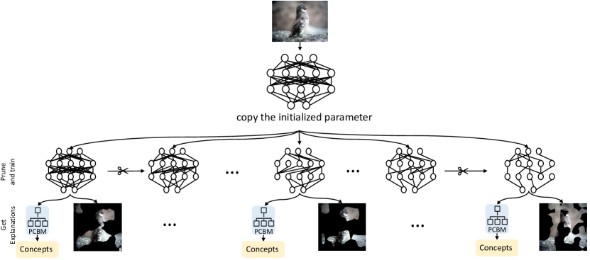
Figure 1: Overview of our method. (1) First, we prune a deep neural network using Lottery Ticket Hypothesis [13]. (2) For each pruned subnetwork, we identify the top human interpretable concepts for classification using PCBM [43]. (3) For each pruned subnetwork, we compute the local explanation using Grad-CAM [33].

In this paper, we study the relationship between pruning and explainability. Initially, we prune the deep model using LTH. We then test either of the following hypotheses: Hypothesis A. The pruned networks prioritize the same relevant concepts/pixels for prediction as the original network. Hence pruning has no effect on the global/local explanations. As a result, LTH is able to identify the winning tickets, i.e. subnetworks with comparable or superior performance to the original network. Hypothesis B. Pruning modifies the global/local explanations as the pruned networks prioritize different concepts/pixels for prediction compared to the original network. Consequently, LTH is unable to find the winning tickets. To validate the two hypotheses, we borrow tools from explainable AI to quantify explanations for different pruned networks. Specifically, we use Grad-CAM to estimate the local explanations and use PCBM to identify the important concepts from the embeddings of each pruned network. To our knowledge, we are the first to investigate the concept-based explainability of LTH using PCBM.

2 Explaining Lottery Ticket Hypothesis

Overview. We train a neural network $\displaystyle f:\mathcal{X}\rightarrow\mathcal{Y}$, taking images $\mathcal{X}$ as input to predict the labels $\mathcal{Y}\in\mathbb{R}^{K}$, $K$ being the number of classes. We assume that $\displaystyle f$ is a composition $\displaystyle h\circ\Phi$, where $\displaystyle\Phi:\mathcal{X}\rightarrow\mathbb{R}^{l}$ is the image embedding and $\displaystyle h:\mathbb{R}^{l}\rightarrow\mathcal{Y}$ is a classifier. Figure 1 shows an overview of our approach.

2.1 Pruning Methodology

LTH [13] aims to find a pruned subnetwork within a deep neural network that achieves similar accuracy as the original network – when trained in isolation. These pruned networks are finetuned for a small number of iterations to achieve accuracy. We prune and fine-tune the network $f$ simultaneously for $n$ rounds using the strategy of iterative magnitude pruning in LTH [13]. Thus we obtain $f^{1},f^{2},\dots,f^{n}$ subnetworks where the network $f$ for the $i^{th}$ round is denoted as $f^{i}(.)=h^{i}(\Phi^{i}(.))$. For brevity, we drop round index $i$ from the notations in the following sections.

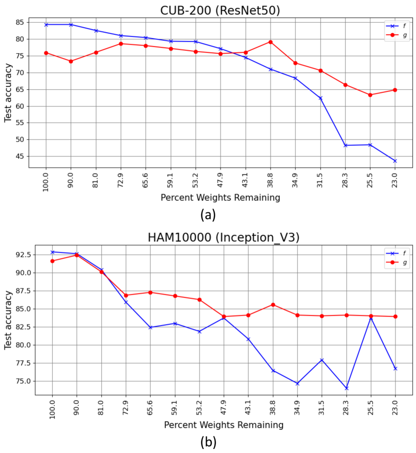
Figure 2: The test accuracy on CUB-200 and HAM10000 when the network is pruned to the specified size.

Table 1: The top-3 concepts with the highest weights of the carved interpretable models ($g$) using PCBM from the pruned subnetworks for various pruning iterations for the bird species of CUB-200 dataset. Due to the space constraint, we only report the concepts from $g$ extracted from the model for iterations 1, 2, 4, and 15 with 100%, 90% 72.9%, and 23% weights remaining.

LABEL	100.0 % WEIGHTS REMAINING	90.0 % WEIGHTS REMAINING	72.9 % WEIGHTS REMAINING	23.0 % WEIGHTS REMAINING
Black footed Albatross	1. bill_shape_hooked_seabird 2. under_tail_color_black 3. size_medium_9_16_in	1. bill_shape_hooked_seabird 2. under_tail_color_black 3. wing_pattern_solid	1. bill_shape_hooked_seabird 2. leg_color_grey 3. size_medium_9_16_in	1. bill_shape_hooked_seabird 2. underparts_color_grey 3. wing_pattern_solid
Rusty Blackbird	1. back_color_brown 2. breast_color_brown 3. wing_color_black	1. underparts_color_buff 2. breast_color_brown 3. back_color_brown	1. breast_color_brown 2. belly_color_grey 3. underparts_color_grey	1. underparts_color_buff 2. back_color_brown 3. belly_color_grey
White Pelican	1. bill_shape_dagger 2. upper_tail_color_white 3. back_pattern_multicolored	1. wing_pattern_solid 2. bill_color_grey 3. upper_tail_color_white	1. belly_color_yellow 2. primary_color_yellow 3. underparts_color_yellow	1. wing_pattern_multicolored 2. bill_color_grey 3. wing_color_white
Grasshopper Sparrow	1. back_color_buff 2. wing_pattern_striped 3. back_pattern_striped	1. back_color_buff 2. wing_pattern_striped 3. belly_color_buff	1. belly_color_buff 2. wing_color_white 3. upperparts_color_buff	1. back_color_buff 2. belly_color_buff 3. underparts_color_buff
Vesper Sparrow	1. leg_color_black 2. nape_color_buff 3. primary_color_buff	1. nape_color_buff 2. primary_color_buff 3. head_pattern_plain	1. nape_color_buff 2. back_color_buff 3. wing_color_buff’	1. under_tail_color_buff 2. breast_color_black 3. wing_color_buff
Heermann Gull	1. breast_color_grey 2. upper_tail_color_black 3. underparts_color_grey	1. breast_color_grey 2. underparts_color_grey 3. throat_color_grey	1. belly_color_grey 2. breast_color_grey 3. underparts_color_grey	1. head_pattern_plain 2. back_color_grey 3. primary_color_grey
American Crow	1. crown_color_grey 2. forehead_color_grey 3. wing_shape_roundedwings	1. wing_shape_roundedwings 2. forehead_color_grey 3. primary_color_grey	1. throat_color_grey 2. wing_shape_roundedwings 3. back_color_grey	1. underparts_color_grey 2. back_color_grey 3. belly_color_black
Winter Wren	1. breast_color_brown 2. forehead_color_brown 3. under_tail_color_brown	1. breast_color_brown 2. underparts_color_brown 3. forehead_color_brown	1. breast_color_brown 2. underparts_color_brown 3. under_tail_color_brown	1. size_very_small_3_5_in 2. forehead_color_brown 3. crown_color_brown
House Sparrow	1. breast_color_grey 2. upperparts_color_black 3. primary_color_brown	1. breast_color_grey 2. primary_color_brown 3. bill_shape_cone	1. bill_shape_cone 2. breast_color_grey 3. nape_color_grey	1. breast_color_grey 2. tail_shape_notched_tail 3. bill_shape_cone
Prothonotary Warbler	1. under_tail_color_grey 2. head_pattern_plain 3. back_pattern_multicolored	1. head_pattern_plain 2. leg_color_grey 3. back_pattern_multicolored	1. back_pattern_multicolored 2. under_tail_color_grey 3. crown_color_yellow	1. nape_color_yellow 2. back_pattern_multicolored 3. crown_color_yellow

2.2 Retrieving the concepts from embeddings

Learn the concept predictor. For datasets with the concept annotation $\mathcal{C}\in\mathbb{R}^{N_{c}}$ ($N_{c}$ being the number of concepts per image $\mathcal{X}$), the learnable $t:R^{l}\rightarrow\mathcal{C}$ classifies the concepts using the embeddings $\Phi$ of each pruned networks. Per this definition, $t$ outputs a scalar value $c$ representing each concept in the concept vector for each input image. For datasets without concept annotation, we leverage a set of image embeddings with the concept being present and absent) [43] and learn a linear SVM ($t$) to construct the concept activation matrix [20] as $\boldsymbol{Q}\in\mathbb{R}^{N_{c}\times l}$. Finally we estimate the concept value as $c=\frac{<\Phi(x),q^{i}>}{||q_{i}||_{2}^{2}}$ $\in\mathbb{R}$ utilizing each row $\boldsymbol{q^{i}}$ of $\boldsymbol{Q}$. Thus, the complete tuple of $j^{th}$ sample is $\{x_{j},y_{j},c_{j}\}$, denoting the image, label, and learned concept vector, respectively.

Learn PCBM. Following [43], we carve the interpretable classifier $g:\mathcal{C}\rightarrow\mathcal{Y}$ from $f$ to predict the labels from the concepts using the following loss:

$$\min_{g}\mathbb{E}_{c,y\sim\mathcal{C},\mathcal{Y}}\big{[}\mathcal{L}(g(c),y)\big{]}+\frac{\lambda}{N_{c}K}\Omega(g),$$ (1)

where $g(c)=w^{T}c+b$, $\lambda$ is the regularization strength, $\Omega$ is the elastic net penalty [43]. $g$ associates each concept with a weight after training, implying its predictive significance to the class labels.

2.3 Local explanations using Grad-CAM

Saliency maps are heatmap-based techniques, highlighting essential features (pixels for images) in the input space responsible for the model’s prediction as a class label $k$. In this paper, we adopt GRAD-CAM method [33]. We calculate the heatmap by choosing an intermediate convolutional layer and then linearizing the rest of the network to be interpretable.

3 Experiments

Table 2: The top-3 concepts with the highest weights of the carved interpretable models ($g$) using PCBM from the pruned subnetworks for various pruning iterations for the HAM10000 dataset. Due to the space constraint, we only report the concepts from $g$ extracted from the model for iterations 1, 2, 4, and 15 with 100%, 90%, 81%, 72.9%, 25.5%, and 23% weights remaining.

LABEL	100.0 % WEIGHTS REMAINING	90.0 % WEIGHTS REMAINING	72.9 % WEIGHTS REMAINING	23.0 % WEIGHTS REMAINING
Malignant	1. BWV 2. IrregularStreaks 3. RegressionStructures	1. AtypicalPigmentNetwork 2. BWV 3. IrregularDG	1. IrregularStreaks 2. lAtypicalPigmentNetwork 3. RegressionStructures	1. AtypicalPigmentNetwork 2. TypicalPigmentNetwork 3. IrregularStreaks
Benign	1. TypicalPigmentNetwork 2. RegularStreaks 3. RegularDG	1. TypicalPigmentNetwork 2. RegressionStructures 3. RegularDG	1. RegularStreaks 2. TypicalPigmentNetwork 3. RegularDG	1. RegularStreaks 2. RegularDG 3. IrregularDG

We perform experiments on CUB-200 [41] and HAM10000 [40] using ResNet [16] and Inception [39] networks, respectively. We prune the networks for 15 iterations, removing 10% of weights in each iteration, fine-tuning, and then pruning again. We conduct three experiments. First, we estimate the accuracy scores to evaluate the predictive performance of the different pruned networks and carved interpretable models. Second, we use interpretable models to estimate the top three concepts. Third, we compute the Grad-CAM-based saliency maps for each pruned network to compare the local explanations qualitatively. In all the subsequent plots, we denote the original network as the one with “100% weight remaining”. We use the entire $\Phi$ as the concept extractor. We describe the dataset and training configurations in detail in the supplementary materials. The code is available at: https://github.com/batmanlab/lth-explain

3.1 Results

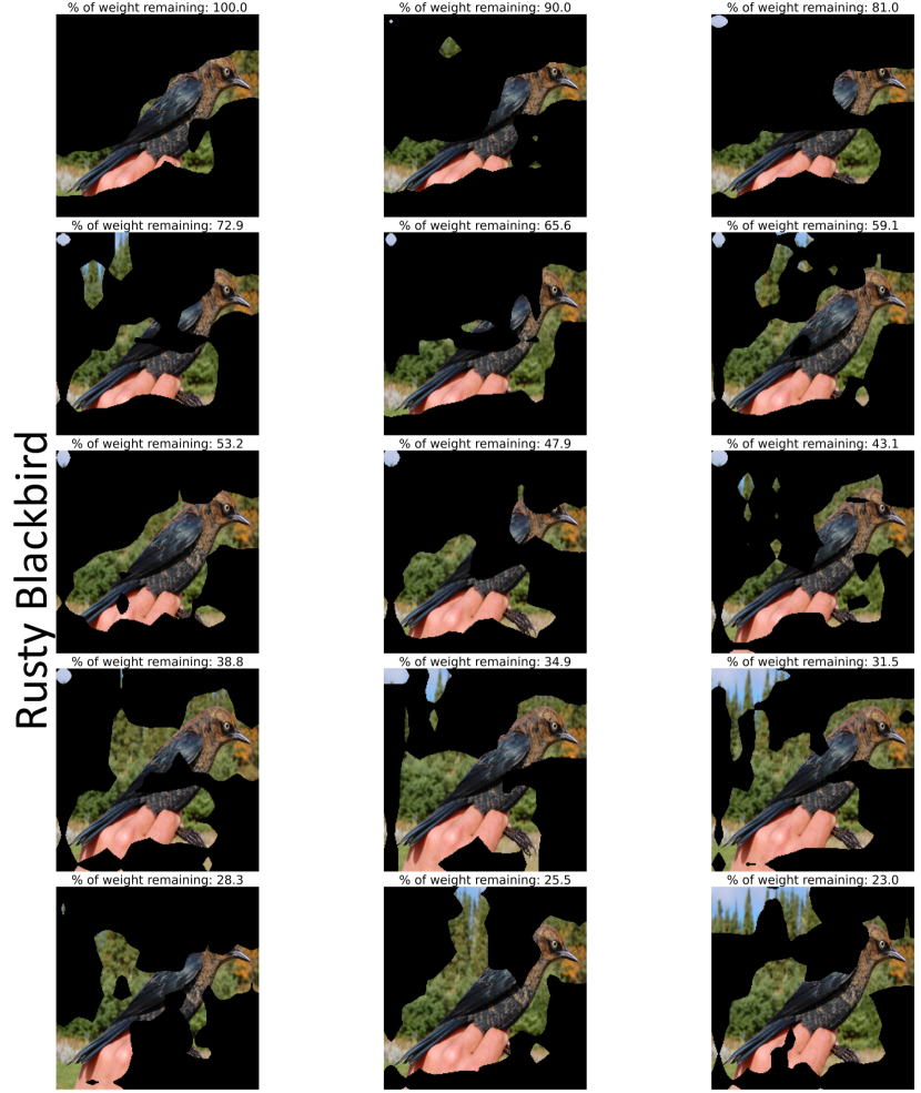
Figure 3: Grad-CAM outputs of “Rusty Blackbird” for various pruned models.

Quantitative evaluation of $\boldsymbol{f}$ and $\boldsymbol{g}$. Fig. 2 shows the accuracies for different pruning iterations for CUB-200 and HAM10000 datasets for the original neural network ($f$) and the carved interpretable model ($g$) using PCBM. As we prune more, the performance of $f$ and $g$ deteriorates. When $\sim$28% weights remain, the accuracy of the $f$ and $g$ drops from 84.8% and 75.7% to 48% and 66% compared to the original networks for CUB-200. Strikingly, for later iterations, $g$ performs better than $f$. As pruning removes irrelevant components from the network, the pruned networks utilize the concepts for the classification.

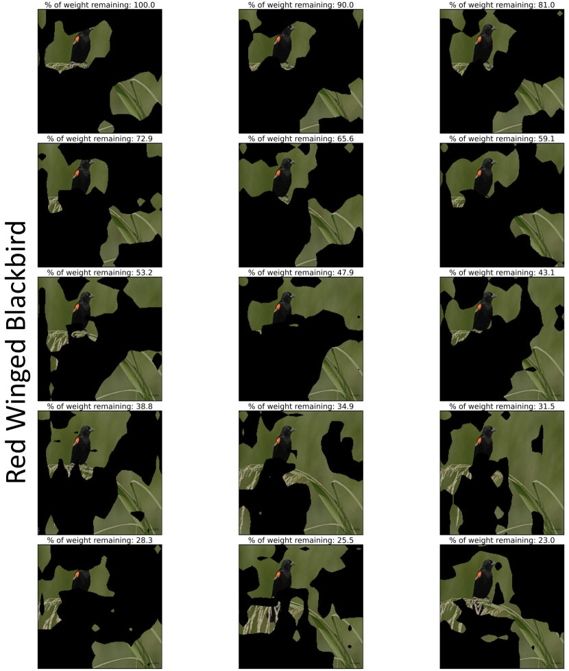
Figure 8: Grad-CAM outputs of “Red Winged Blackbird” for various pruned models.

Explaining LTH. Tab. 3 and 2 reports the top-3 concepts for the different interpretable models $g$ for each pruned networks from $f$ for CUB-200 and HAM10000, respectively. After training, $g$ associates each concept with a weight. A concept with a high weight implies its high predictive significance. Tab. 3 and 2 demonstrate that different pruned networks rely on different concepts for classifying the same class labels. For example, the initial network with 100% weights relies on breast_color_grey, upperparts_color_black and primary_color_brown as top-3 concepts for the bird species “House Sparrow”. However, when 23% of the weights remained in the network, the classification of “House Sparrow” relies on tail_shape_notched_tail and bill_shape_cone in addition to breast_color_grey. For HAM10000, the initial networks with 100% weights identifies Blue Whitish Veil (BWV), IrregularStreaks and RegressionStructures as top-3 concepts for Malignant skin lesion. These concepts are clinically relevant for malignancy [27, 25]. However, the network with 23% weights identifies clinically irrelevant TypicalPignmentNetwork as one of the identifying concepts for malignancy.  Fig. 8 shows similar inconsistencies in the Grad-CAM outputs for different networks. The network with 100% weights focuses on the relevant pixels on the bird’s body, but the network with $\sim$ 23% weights also highlights the background as relevant pixels. These findings demonstrate that drastic pruning alters the network’s representation, resulting in a performance decrease. For more results, refer to the supplementary materials.

4 Conclusion & Future Work

In this paper, we study the success/failure modes of LTH using explainability with concepts and pixels. We observe that the pruned networks using LTH with more weights highlight relevant concepts and pixels; the networks with fewer weights do not. As a result, we conclude that magnitude iterative pruning does not emphasize the relevant concepts or pixels as the original model; in fact, the opposite is true. In the future, we want to extend this study to more real-life chest-x-ray datasets, eg. MIMIC-CXR [18]. Also, we want to employ Route, interpret and repeat [14] algorithm to rank the samples based on the difficulty and investigate whether the extracted concepts differ significantly for "harder" samples as we prune. Also, a teacher-student framework can be employed where the original network and the subsequent pruned networks will be considered as teacher and student respectively. The saliency maps of the teacher model will ensure the student model focuses on the relevant pixels even with the limited network capacity.

Supplementary materials

5 Reproduciblity

The code is available at: https://github.com/batmanlab/lth-explain.

6 Related Work

Network pruning

In practice, neural networks are frequently overparameterized. Distillation [5, 17] and pruning [23, 15] both rely on the ability to reduce parameters while maintaining accuracy. Even with adequate memory capacity for training data, networks naturally learn more specific functions [45, 29, 4] Later research shows that the overparameterized networks are easier to train [8, 17, 46]. Recently Lottery Ticket Hypothesis [13] aims to find a subnetwork within a deep neural net performs similarly or even better as the original deep network.

Saliency map based explanation methods

First [35] developed a saliency map technique to highlight the relevant pixels in the image for the model’s prediction. In CAM [46], we take the global average pooling of the feature map from the final convolution layer. Then we train a linear classifier to get the weights corresponding to each feature map, denoting the importance of a feature map to the final prediction. Later in [33, 9, 37, 38] amalgamate the gradient information with relevant weights of the necessary pixels to generate more localized saliency maps. In summary, the saliency maps aim to provide local explanations in terms of pixels. However, these saliency maps are often criticized for being inconsistent  [30]. [2, 21] demonstrates that the saliency maps highlight the correct regions in the image even though the backbone’s representation was arbitrarily perturbed. The explanations in terms of pixel intensities do not correspond to the high-level interpretable concept, understood by humans. In this project, we also aim to provide the post hoc explanation of the all the pruned models in terms of the interpretable concepts as a global explanation, rather than the pixel intensities.

Concept-based explanation methods

In concept based explanation methods, researchers aim to quantify the importance of a humanly interpretable concept for the model’s prediction. In TCAV [20], the researchers first learn the concept activation vectors (CAV) by learning a linear classifier that separates the concept images and the random images. After that, they estimate the TCAV score by taking the derivative of the prediction probabilities w.r.t. the concept activation vectors. In the concept completeness paper [42], they derived a metric known as the “concept completeness score”, which shows whether the given concepts are sufficient to explain the prediction of the black box. In the Network, dissection method [7], the activations of each unit are segmented to find its association with a given concept by taking the intersection over the union metric. Recently, in [11], the researchers relax the assumption in [20] that concepts are linearly separable in the latent space; instead, they are represented by clusters, and the researchers obtain the concepts by utilizing the gaussian kernels for SVM based classifier. Also [22] proposes the interpretable-by-design approcach “Concept Bottleneck Models (CBMs)”, which predicts the concepts from the images and then the labels from the predicted concepts. Several modifications to the original CBM model are discussed [32, 44, 26]. Later [43] proposes Post-hoc Concept Bottleneck Models (PCBMs), where they identify the concepts from the embeddings of a pre-trained model. Recently [14] introduces Route, Interpret, and Repeat where they carve out a mixture of interpretable models from a pre-trained neural network.

In this short paper, we want to study the explainability in terms of both the human interpretable concepts and pixels for the pruned subnetworks using LTH using PCBM and Grad-CAM, respectively.

7 Background on LTH

LTH [13] aims to find a subnetwork within a deep neural network that achieves similar accuracy as the original network – when trained in isolation. Specifically, we perform the following steps to train and prune the smallest magnitude weights of the neural network $f$:

1. Randomly initialize $f(.;\theta_{0})$ (where $\theta_{0}\sim\mathcal{D_{\theta}}$).

2. Prune $p\%$ of the parameters $\theta_{j}$ with smallest magnitude weights, creating a mask $m$.

3. Optimize the network for $j$ iterations using stochastic gradient descent (SGD) on a training set, arriving at parameters $\theta_{j}$.

4. Reset the remaining parameters to their values in $\theta_{0}$, creating a subnetwork $f(x;m\odot\theta_{0})$.

5. Finetune and continue pruning for $n$ rounds obtaining $n$-pruned subnetworks.

As pruning gradually reduces the network in size, we measure the performance and explainability for the all $n$-pruned subnetworks.

8 Background on Grad-CAM

Saliency maps are heatmap-based techniques, highlighting important features (pixels for images) in the input space responsible for the model’s prediction as a class label $k$. In this project, we utilize GRAD-CAM method [33]. We calculate the heatmap by choosing an intermediate convolutional layer and then linearizing the rest of the network to be interpretable. Specifically, we estimate the derivative of the predicted output w.r.t. each channel of the convolutional layer averaged over all spatial locations as follows:

$$w^{m}_{k}=\sum_{i}\sum_{j}\frac{\partial Y^{k}}{\partial A_{i,j}^{m}}\text{,}$$ (2)

where $w^{k}_{c}$ is the weight for $k^{th}$ class and $m^{th}$ feature map, $Y^{k}$ is the prediction for $k^{th}$ class and $A_{i,j}^{m}$ is the ${i,j}^{th}$ location of $m^{th}$ feature map. This results in a scalar for each channel that captures the importance of that channel in making the current prediction. Then, we calculate a weighted average of all activations of the convolutional layer with the above-importance weights for each channel to get a 2D matrix over spatial locations Finally, we keep only positive numbers and resize them to the size of an input image to get the interpretation heatmap $e$. In this project, corresponding to an image, we estimate this heatmap for all the $n$-pruned networks.

9 Dataset

CUB-200. The Caltech-UCSD Birds-200-2011 [41] is a fine-grained classification dataset comprising 11788 images and 312 noisy visual concepts to classify the correct bird species from 200 possible classes. We adopted the strategy [6] to extract 108 denoised visual concepts. Also, we utilize training/validation splits from [6].

HAM10000 HAM10000 ([40]) is a classification dataset aiming to classify a skin lesion as benign or malignant. We follow the strategy in [25] to extract the 8 concepts from the Derm7pt ([19]) dataset.

10 Training configurations

Configurations of LTH We utilize ResNet50 [16] and Inception-V3 [39] as the main neural network model to be pruned for CUB-200 and HAM10000 datasets, respectively. In each pruning iteration, we prune 10% of the weights, and we prune it for 15 iterations. We resize the images to 448$\times$448 and 299$\times$299 for CUB-200 and HAM-10000, respectively. We set a batch size of 32 and utilized Stochastic gradient descent with a learning rate of 0.01 to train the main network and finetune the pruned subnetworks.

Configurations of concept extractor We use all the convolution blocks of ResNet-50 and Inception-V3 as image embeddings. We flatten the image embeddings using adaptive average pooling to train the concept extractor $t$. For CUB-200, we train a SGD classifier for 15 epochs with a learning rate of 0.01. Lastly for HAM-10000, we train a linear SVM classifier to extract the concepts from the Derm7pt dataset. We use 50 images each of samples with and without the disease to train the SVM classifier.

Training PCBM The interpretable model $g$ of PCBM is an SGD classifier, trained for 35 epochs with a learning rate of 0.01.

Table 3: The top-3 concepts with the highest weights of the carved interpretable models ($g$) using PCBM from the pruned subnetworks for various pruning iterations for the bird species of the CUB-200 dataset. Due to the space constraint, we only report the concepts from $g$ extracted from the model for iterations 1, 2, 4, and 15 with 100%, 90%, 72.9%, and 23% weights remaining.

LABEL	100.0 % WEIGHTS REMAINING	90.0 % WEIGHTS REMAINING	72.9 % WEIGHTS REMAINING	23.0 % WEIGHTS REMAINING
Cerulean Warbler	1. forehead_color_blue 2. crown_color_blue 3. nape_color_blue	1. forehead_color_blue 2. nape_color_blue 3. crown_color_blue	1. crown_color_blue 2. nape_color_blue 3. size_very_small_3_5_in	1. size_very_small_3_5_in 2. nape_color_blue 3. forehead_color_blue
Rock Wren	1. breast_color_buff 2. belly_color_buff 3. underparts_color_grey	1. belly_color_buff 2. breast_color_buff 3. upperparts_color_grey	1. belly_color_buff 2. breast_color_buff 3. throat_color_grey	1. breast_color_grey 2. belly_color_buff 3. leg_color_black
Loggerhead Shriker	1. tail_pattern_multicolored 2. forehead_color_grey 3. crown_color_grey	1. forehead_color_grey 2. crown_color_grey 3. leg_color_black	1.crown_color_grey 2. forehead_color_grey 3. head_pattern_capped	1. forehead_color_grey 2. leg_color_black 3. primary_color_buff
Philadelphia Vireo	1. size_very_small_3_5_in 2. under_tail_color_grey 3. leg_color_grey	1. size_very_small_3_5_in 2. leg_color_grey 3. forehead_color_grey	1. primary_color_buff 2. under_tail_color_grey 3. size_very_small_3_5_in	1. crown_color_grey 2.leg_color_grey 3. under_tail_color_grey
Tennessee Warbler	1. bill_color_grey 2. wing_color_yellow 3. leg_color_grey	1. under_tail_color_grey 2. bill_color_grey 3. wing_color_yellow	1. bill_color_grey 2. under_tail_color_grey 3. forehead_color_yellow	1. bill_color_grey 2. leg_color_grey 3. forehead_color_yellow
Palm Warbler	1. wing_pattern_striped 2. wing_shape_roundedwings 3. leg_color_black	1. wing_pattern_striped 2. throat_color_yellow 3. bill_shape_allpurpose	1. wing_pattern_striped 2. throat_color_yellow 3. bill_shape_allpurpose	1. wing_pattern_striped 2. wing_shape_roundedwings 3. bill_shape_allpurpose
Mourning Warbler	1. leg_color_buff 2. under_tail_color_grey 3. throat_color_grey	1. crown_color_black 2. throat_color_grey 3. forehead_color_black	1. under_tail_color_yellow 2. leg_color_buff 3. crown_color_black	1. leg_color_buff 2. wing_color_yellow 3. wing_pattern_solid
Wilson Warbler	1. crown_color_black 2. under_tail_color_yellow 3. head_pattern_capped	1. crown_color_black 2. nape_color_yellow 3. under_tail_color_yellow	1. under_tail_color_yellow 2. crown_color_black 3. head_pattern_plain	1. under_tail_color_yellow 2. size_very_small_3_5_in 3. back_color_yellow
Cactus Wren	1. belly_color_buff 2. breast_color_black 3. underparts_color_buff	1. breast_color_black 2. underparts_color_buff 3. bill_length_about_same_as_head	1. underparts_color_buff 2. bill_length_about_same_as_head 3. breast_color_black	1. bill_shape_dagger 2. belly_color_buff 3. leg_color_black
Elegant Tern	1. bill_shape_dagger 2. head_pattern_capped 3. wing_color_grey	1. bill_shape_dagger 2. head_pattern_capped 3. back_color_white	1. bill_shape_dagger 2. back_color_white 3. head_pattern_capped	1. bill_shape_dagger 2. head_pattern_capped 3. back_color_white
Savannah Sparrow	1. breast_pattern_striped 2. tail_shape_notched_tail 3. throat_color_yellow	1. breast_pattern_striped 2. breast_color_black 3. crown_color_black	1. breast_pattern_striped 2. throat_color_yellow 3. breast_color_black	1. breast_pattern_striped 2. breast_color_black 3. under_tail_color_buff
Louisiana Waterthrush	1. wing_pattern_solid 2. back_pattern_solid 3. underparts_color_white	1. breast_pattern_striped 2. wing_pattern_solid 3. throat_color_black	1. leg_color_buff 2. wing_pattern_solid 3. breast_pattern_striped	1. tail_pattern_solid 2. belly_color_white 3. breast_color_white
Cape May Warbler	1. breast_pattern_striped 2. breast_color_black 3. wing_pattern_striped	1. breast_pattern_striped 2. breast_color_black 3. tail_shape_notched_tail	1. underparts_color_black 2. tail_shape_notched_tail 3. breast_color_black	1. wing_pattern_striped 2. tail_shape_notched_tail 3. underparts_color_black
Cliff Swallow	1. belly_color_buff 2. underparts_color_buff 3. bill_shape_cone	1. underparts_color_buff 2. belly_color_buff 3. bill_shape_cone	1. belly_color_buff 2. underparts_color_buff 3. bill_shape_cone	1. belly_color_buff 2. underparts_color_buff 3. bill_color_black
Caspian Tern	1. leg_color_black 2. tail_pattern_solid 3. upper_tail_color_white	1. tail_pattern_solid 2. leg_color_black 3. forehead_color_red	1. leg_color_black 2. tail_pattern_solid 3. crown_color_black	1. bill_shape_dagger 2. head_pattern_capped 3. leg_color_black
Red eyed Vireo	1. upper_tail_color_grey 2. forehead_color_yellow 3. back_pattern_solid	1. throat_color_white 2. upper_tail_color_grey 3. forehead_color_yellow	1. bill_color_grey 2. tail_pattern_multicolored 3. forehead_color_grey	1. forehead_color_yellow 2. underparts_color_white 3. breast_pattern_solid
Chestnut sided Warbler	1. crown_color_yellow 2. forehead_color_yellow 3. upper_tail_color_grey	1. forehead_color_yellow 2. crown_color_yellow 3. upper_tail_color_grey	1. forehead_color_yellow 2. crown_color_yellow 3. back_pattern_striped	1. crown_color_yellow 2. wing_color_white 3. tail_shape_notched_tail’
Green tailed Towhee	1. belly_color_grey 2. bill_color_grey 3. wing_color_yellow	1. belly_color_grey 2. underparts_color_grey 3. wing_color_yellow	1. underparts_color_grey 2. bill_color_grey 3. belly_color_grey	1. underparts_color_grey 2. wing_color_yellow 3. belly_color_grey
Kentucky Warbler	1. leg_color_buff 2. crown_color_black 3. throat_color_yellow	1. leg_color_buff 2. crown_color_black 3. throat_color_yellow	1. leg_color_buff 2. forehead_color_black 3. crown_color_black	1. wing_color_yellow 2. leg_color_buff 3. under_tail_color_yellow
Forsters Tern	1. head_pattern_capped 2. bill_shape_dagger 3. nape_color_black	1. head_pattern_capped 2. bill_shape_dagger 3. forehead_color_black	1. breast_color_grey 2. head_pattern_capped 3. crown_color_black	1. head_pattern_capped 2. bill_shape_dagger 3. crown_color_black
Mourning Warbler	1. leg_color_buff 2. crown_color_black 3. throat_color_grey	1. crown_color_black 2. throat_color_grey 3. forehead_color_black	1. under_tail_color_yellow 2. leg_color_buff 3. crown_color_black	1. leg_color_buff 2. wing_color_yellow 3. wing_pattern_solid
Clark Nutcracker	1. breast_color_grey 2. upper_tail_color_black 3. primary_color_grey	1. breast_color_grey 2. under_tail_color_white 3. wing_pattern_multicolored	1. underparts_color_grey 2. under_tail_color_white 3. primary_color_grey	1. breast_color_grey 2. throat_color_grey 3. belly_color_grey
Hooded Oriole	1. tail_pattern_multicolored 2. throat_color_black 3. wing_pattern_multicolored	1. leg_color_grey 2. back_color_yellow 3. wing_pattern_multicolored	1. leg_color_grey 2. wing_color_white 3. wing_pattern_multicolored	1. leg_color_grey 2. wing_pattern_multicolored 3. head_pattern_plain
Gray Catbird	1. throat_color_grey 2. head_pattern_capped 3. upper_tail_color_grey	1. upper_tail_color_grey 2. throat_color_grey 3. back_color_grey	1. throat_color_grey 2. primary_color_grey 3. under_tail_color_grey	1. throat_color_grey 2. back_color_grey 3. wing_pattern_solid

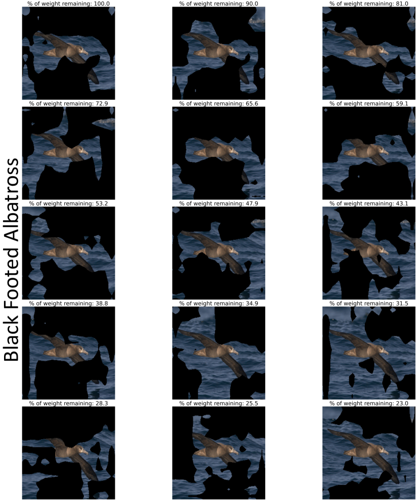
Figure 4: Grad-CAM outputs of “Black Footed Albatross” for various pruned models.

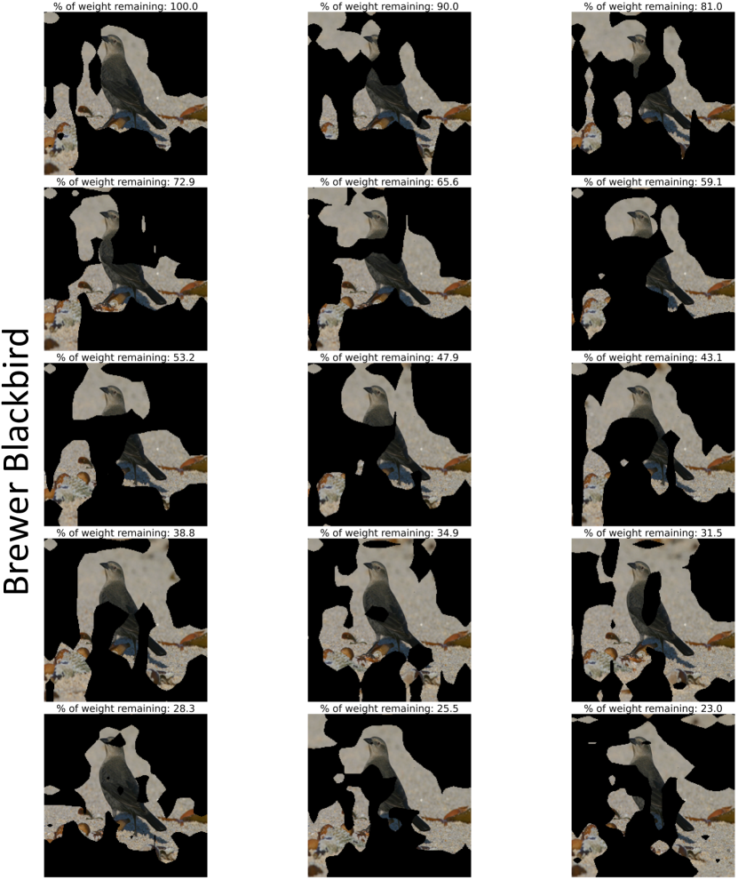
Figure 5: Grad-CAM outputs of “Brewer Blackbird” for various pruned models.

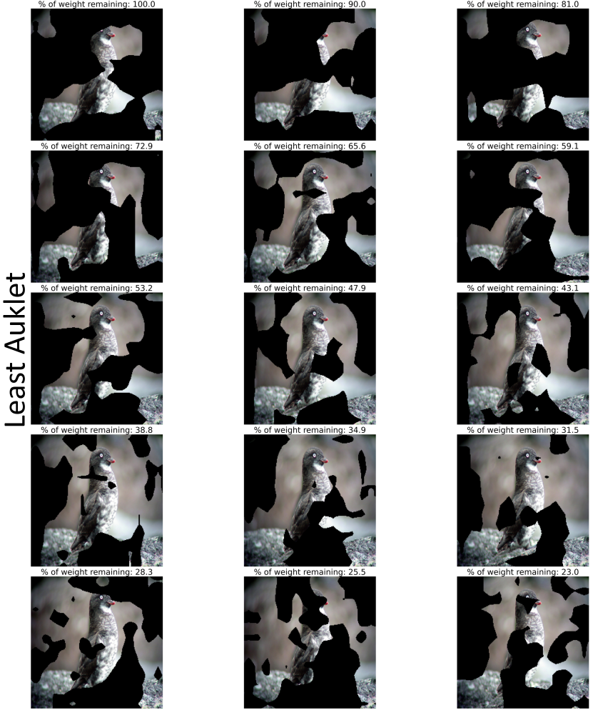
Figure 6: Grad-CAM outputs of “Least Auklet” for various pruned models.

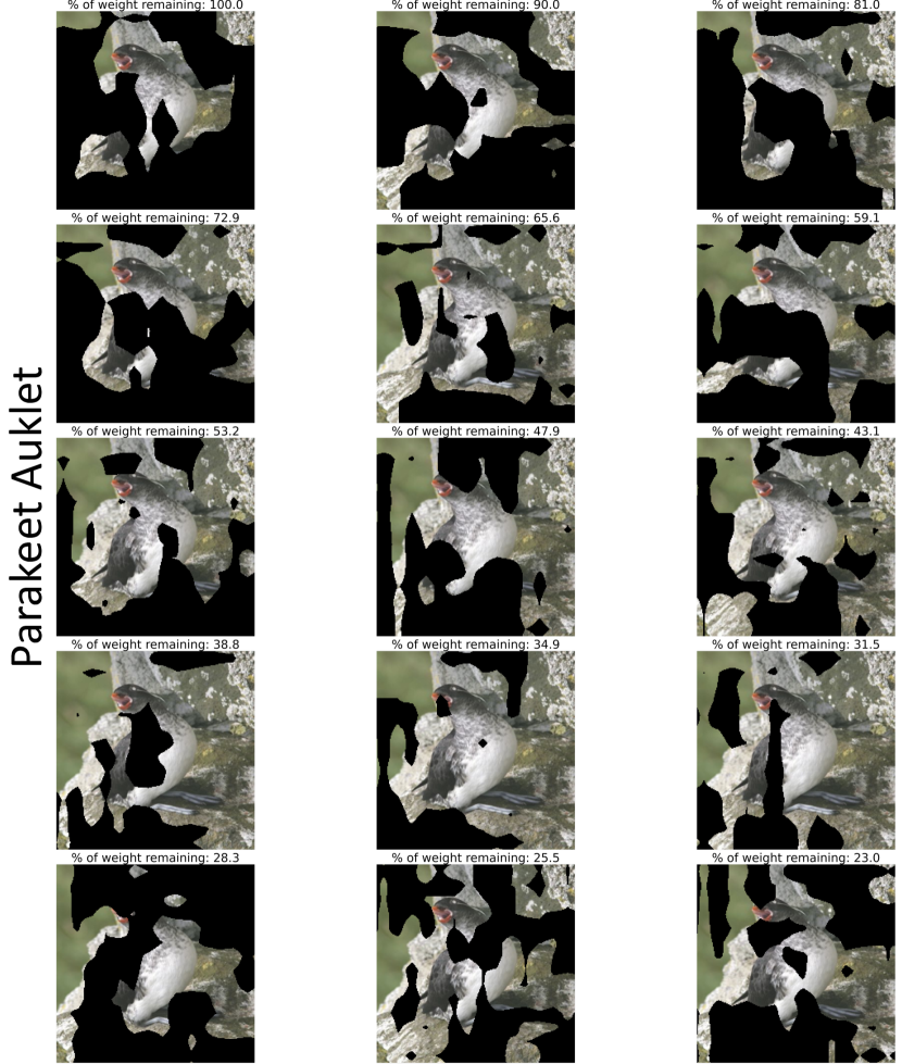
Figure 7: Grad-CAM outputs of “Parakeet Auklet” for various pruned models.

References

- [1] Abubakar Abid, Mert Yuksekgonul, and James Zou. Meaningfully explaining model mistakes using conceptual counterfactuals. arXiv preprint arXiv:2106.12723, 2021.
- [2] Julius Adebayo, Justin Gilmer, Michael Muelly, Ian Goodfellow, Moritz Hardt, and Been Kim. Sanity checks for saliency maps. Advances in neural information processing systems, 31, 2018.
- [3] Raed Alharbi, Minh N Vu, and My T Thai. Learning interpretation with explainable knowledge distillation. In 2021 IEEE International Conference on Big Data (Big Data), pages 705–714. IEEE, 2021.
- [4] Devansh Arpit, Stanisław Jastrzębski, Nicolas Ballas, David Krueger, Emmanuel Bengio, Maxinder S Kanwal, Tegan Maharaj, Asja Fischer, Aaron Courville, Yoshua Bengio, et al. A closer look at memorization in deep networks. In International conference on machine learning, pages 233–242. PMLR, 2017.
- [5] Jimmy Ba and Rich Caruana. Do deep nets really need to be deep? Advances in neural information processing systems, 27, 2014.
- [6] Pietro Barbiero, Gabriele Ciravegna, Francesco Giannini, Pietro Lió, Marco Gori, and Stefano Melacci. Entropy-based logic explanations of neural networks. In Proceedings of the AAAI Conference on Artificial Intelligence, volume 36, pages 6046–6054, 2022.
- [7] David Bau, Bolei Zhou, Aditya Khosla, Aude Oliva, and Antonio Torralba. Network dissection: Quantifying interpretability of deep visual representations. In Proceedings of the IEEE conference on computer vision and pattern recognition, pages 6541–6549, 2017.
- [8] Yoshua Bengio, Nicolas Roux, Pascal Vincent, Olivier Delalleau, and Patrice Marcotte. Convex neural networks. Advances in neural information processing systems, 18, 2005.
- [9] Adiya Chattopadhyay, Anirban Sarkar, Prantik Howlader, and Vineeth N Balasubramanian. Grad-cam: Improved visual explanations for deep convolutional networks. arXiv: 1710.11063, 2017.
- [10] Xu Cheng, Zhefan Rao, Yilan Chen, and Quanshi Zhang. Explaining knowledge distillation by quantifying the knowledge. In Proceedings of the IEEE/CVF conference on computer vision and pattern recognition, pages 12925–12935, 2020.
- [11] Jonathan Crabbé and Mihaela van der Schaar. Concept activation regions: A generalized framework for concept-based explanations. arXiv preprint arXiv:2209.11222, 2022.
- [12] Jonathan Frankle and David Bau. Dissecting pruned neural networks. arXiv preprint arXiv:1907.00262, 2019.
- [13] Jonathan Frankle and Michael Carbin. The lottery ticket hypothesis: Finding sparse, trainable neural networks. arXiv preprint arXiv:1803.03635, 2018.
- [14] Shantanu Ghosh, Ke Yu, Forough Arabshahi, and Kayhan Batmanghelich. Route, interpret, repeat: Blurring the line between post hoc explainability and interpretable models. arXiv preprint arXiv:2302.10289, 2023.
- [15] Song Han, Jeff Pool, John Tran, and William Dally. Learning both weights and connections for efficient neural network. Advances in neural information processing systems, 28, 2015.
- [16] Kaiming He, Xiangyu Zhang, Shaoqing Ren, and Jian Sun. Deep residual learning for image recognition. In Proceedings of the IEEE conference on computer vision and pattern recognition, pages 770–778, 2016.
- [17] Geoffrey Hinton, Oriol Vinyals, Jeff Dean, et al. Distilling the knowledge in a neural network. arXiv preprint arXiv:1503.02531, 2(7), 2015.
- [18] Alistair EW Johnson, Tom J Pollard, Nathaniel R Greenbaum, Matthew P Lungren, Chih-ying Deng, Yifan Peng, Zhiyong Lu, Roger G Mark, Seth J Berkowitz, and Steven Horng. Mimic-cxr-jpg, a large publicly available database of labeled chest radiographs. arXiv preprint arXiv:1901.07042, 2019.
- [19] Jeremy Kawahara, Sara Daneshvar, Giuseppe Argenziano, and Ghassan Hamarneh. Seven-point checklist and skin lesion classification using multitask multimodal neural nets. IEEE journal of biomedical and health informatics, 23(2):538–546, 2018.
- [20] B Kim, M Wattenberg, J Gilmer, C Cai, J Wexler, F Viegas, et al. Interpretability beyond feature attribution: quantitative testing with concept activation vectors (tcav). arxiv. arXiv preprint arXiv:1711.11279, 2017.
- [21] Pieter-Jan Kindermans, Sara Hooker, Julius Adebayo, Maximilian Alber, Kristof T Schütt, Sven Dähne, Dumitru Erhan, and Been Kim. The (un) reliability of saliency methods. arxiv e-prints, page. arXiv preprint arXiv:1711.00867, 2017.
- [22] Pang Wei Koh, Thao Nguyen, Yew Siang Tang, Stephen Mussmann, Emma Pierson, Been Kim, and Percy Liang. Concept bottleneck models. In International Conference on Machine Learning, pages 5338–5348. PMLR, 2020.
- [23] Yann LeCun, John Denker, and Sara Solla. Optimal brain damage. Advances in neural information processing systems, 2, 1989.
- [24] Hao Li, Asim Kadav, Igor Durdanovic, Hanan Samet, and Hans Peter Graf. Pruning filters for efficient convnets. arXiv preprint arXiv:1608.08710, 2016.
- [25] Adriano Lucieri, Muhammad Naseer Bajwa, Stephan Alexander Braun, Muhammad Imran Malik, Andreas Dengel, and Sheraz Ahmed. On interpretability of deep learning based skin lesion classifiers using concept activation vectors. In 2020 international joint conference on neural networks (IJCNN), pages 1–10. IEEE, 2020.
- [26] Emanuele Marconato, Andrea Passerini, and Stefano Teso. Glancenets: Interpretabile, leak-proof concept-based models. arXiv preprint arXiv:2205.15612, 2022.
- [27] SW Menzies, C Ingvar, and WH McCarthy. A sensitivity and specificity analysis of the surface microscopy features of invasive melanoma. Melanoma research, 6(1):55–62, 1996.
- [28] Grégoire Montavon, Wojciech Samek, and Klaus-Robert Müller. Methods for interpreting and understanding deep neural networks. Digital signal processing, 73:1–15, 2018.
- [29] Behnam Neyshabur, Ryota Tomioka, and Nathan Srebro. In search of the real inductive bias: On the role of implicit regularization in deep learning. arXiv preprint arXiv:1412.6614, 2014.
- [30] Vipin Pillai, Soroush Abbasi Koohpayegani, Ashley Ouligian, Dennis Fong, and Hamed Pirsiavash. Consistent explanations by contrastive learning. In Proceedings of the IEEE/CVF Conference on Computer Vision and Pattern Recognition, pages 10213–10222, 2022.
- [31] Wojciech Samek, Alexander Binder, Grégoire Montavon, Sebastian Lapuschkin, and Klaus-Robert Müller. Evaluating the visualization of what a deep neural network has learned. IEEE transactions on neural networks and learning systems, 28(11):2660–2673, 2016.
- [32] Anirban Sarkar, Deepak Vijaykeerthy, Anindya Sarkar, and Vineeth N Balasubramanian. Inducing semantic grouping of latent concepts for explanations: An ante-hoc approach. arXiv preprint arXiv:2108.11761, 2021.
- [33] RR Selvaraju, M Cogswell, A Das, R Vedantam, D Parikh, and D Batra. Grad-cam: visual explanations from deep networks via gradient-based localization. 2016. arXiv preprint arXiv:1610.02391, 2016.
- [34] Avanti Shrikumar, Peyton Greenside, Anna Shcherbina, and Anshul Kundaje. Not just a black box: Learning important features through propagating activation differences. arXiv preprint arXiv:1605.01713, 2016.
- [35] Karen Simonyan, Andrea Vedaldi, and Andrew Zisserman. Deep inside convolutional networks: Visualising image classification models and saliency maps. arXiv preprint arXiv:1312.6034, 2013.
- [36] Sumedha Singla, Brian Pollack, Junxiang Chen, and Kayhan Batmanghelich. Explanation by progressive exaggeration. arXiv preprint arXiv:1911.00483, 2019.
- [37] Daniel Smilkov, Nikhil Thorat, Been Kim, Fernanda Viégas, and Martin Wattenberg. Smoothgrad: removing noise by adding noise. arXiv preprint arXiv:1706.03825, 2017.
- [38] Mukund Sundararajan, Ankur Taly, and Qiqi Yan. Axiomatic attribution for deep networks. In International conference on machine learning, pages 3319–3328. PMLR, 2017.
- [39] Christian Szegedy, Wei Liu, Yangqing Jia, Pierre Sermanet, Scott Reed, Dragomir Anguelov, Dumitru Erhan, Vincent Vanhoucke, and Andrew Rabinovich. Going deeper with convolutions. In Proceedings of the IEEE conference on computer vision and pattern recognition, pages 1–9, 2015.
- [40] Philipp Tschandl, Cliff Rosendahl, and Harald Kittler. The ham10000 dataset, a large collection of multi-source dermatoscopic images of common pigmented skin lesions. Scientific data, 5(1):1–9, 2018.
- [41] Catherine Wah, Steve Branson, Peter Welinder, Pietro Perona, and Serge Belongie. The caltech-ucsd birds-200-2011 dataset. 2011.
- [42] Chih-Kuan Yeh, Been Kim, Sercan Arik, Chun-Liang Li, Pradeep Ravikumar, and Tomas Pfister. On concept-based explanations in deep neural networks. 2019.
- [43] Mert Yuksekgonul, Maggie Wang, and James Zou. Post-hoc concept bottleneck models. arXiv preprint arXiv:2205.15480, 2022.
- [44] Mateo Espinosa Zarlenga, Pietro Barbiero, Gabriele Ciravegna, Giuseppe Marra, Francesco Giannini, Michelangelo Diligenti, Zohreh Shams, Frederic Precioso, Stefano Melacci, Adrian Weller, et al. Concept embedding models. arXiv preprint arXiv:2209.09056, 2022.
- [45] Chiyuan Zhang, Samy Bengio, Moritz Hardt, Benjamin Recht, and Oriol Vinyals. Understanding deep learning (still) requires rethinking generalization. Communications of the ACM, 64(3):107–115, 2021.
- [46] Bolei Zhou, Aditya Khosla, Agata Lapedriza, Aude Oliva, and Antonio Torralba. Learning deep features for discriminative localization. In Proceedings of the IEEE conference on computer vision and pattern recognition, pages 2921–2929, 2016.