Single reference treatment of strongly correlated H₄ and H₁₀ isomers with Richardson-Gaudin states

Abstract

Richardson-Gaudin (RG) states are employed as a variational wavefunction ansatz for strongly correlated isomers of H₄ and H₁₀. In each case a single RG state describes the seniority-zero sector quite well. Simple natural orbital functionals offer a cheap and reasonable approximation of the outstanding weak correlation in the seniority-zero sector, while systematic improvement is achieved by performing a configuration interaction (CI) in terms of RG states. Other pair theories (e.g. generalized valence bond and pair-coupled-cluster doubles) can provide a good description of many of the geometries considered, but, at short distances, the wavefunctions for the 2D and 3D structures of H₁₀ take the form of an RG state that cannot be described by these other theories.

Université Laval] Département de chimie, Université Laval, Québec, Québec, Canada Florida State University]Department of Chemistry and Biochemistry, Florida State University, Tallahassee, FL 32306-4390 IR,NMR,UV

1 Introduction

Many problems in electronic structure theory can be treated as systems of weakly correlated electrons. In such cases, a single Slater determinant provides a qualitative description of the wavefunction and a short expansion in Slater determinants provides quantitative accuracy. For weakly-correlated systems Kohn-Sham density functional theory (DFT) and coupled-cluster (CC) theory^{1, 2, 3, 4} with singles and doubles⁵ can be expected to predict physically correct results.

Strongly-correlated systems are another story. The wavefunction has no single dominant Slater determinant, and even a qualitative description of the system can become complicated. The standard approach for dealing with strong correlation is the complete active space self-consistent field (CASSCF) approach^{6, 7, 8, 9} which works well if a compact active space of chemically important orbitals can be identified. Even then, active spaces beyond 22 electrons in 22 orbitals¹⁰ are intractable, which has led to the development of a large number of configuration interaction (CI) based schemes as approximate CASSCF solvers,^{11, 12, 13, 14, 15, 16, 17, 18, 19} as well as alternative representations of the electronic structure of the active space that abandon the CI framework altogether.^{20, 21, 22, 23, 24, 25, 26}

It has long been understood²⁷ that two-electron functions, called geminals, describing pairs of weakly-interacting electrons, can provide a better basis for strongly-correlated electrons than Slater determinants of single-particle orbitals. For systems of paired electrons, an excellent description is obtained with the antisymmetrized product of interacting geminals (APIG), but this treatment is completely intractable in practice.^{28, 29, 30, 31, 32, 33, 34} For attractive pairing interactions, such as in the Bardeen-Cooper-Schrieffer (BCS) mechanism^{35, 36, 37} and in nuclear structure, the antisymmetrized geminal power (AGP) gives qualitatively correct results for a meagre cost.^{38, 39, 40, 41, 42, 43, 44, 45, 46} For repulsive interactions, as arise in chemistry, AGP is qualitatively incorrect and requires the use of Jastrow factors to be size-consistent.^{47, 48, 49} Correct understanding of repulsive systems is possible with the antisymmetrized product of strongly-orthogonal geminals (APSG)^{50, 51} and in particular generalized valence bond/perfect pairing (GVB).^{52, 53, 54, 55, 56, 57, 58, 59, 60, 61, 62, 63, 64, 65, 66, 67, 68} These last two approaches require splitting the orbitals into disjoint subspaces, which can be done quite easily by looking at the corresponding unrestricted Hartree-Fock (UHF) orbitals.⁶⁹ Finally, the antisymmetrized product of 1-reference orbital geminals (AP1roG),⁷⁰ which is equivalent to pair-coupled-cluster doubles (pCCD)⁷¹ has shown good results for ground state properties,^{72, 73, 74, 75, 76, 77, 78, 79, 80, 81, 82, 83, 84, 85, 86, 87} and even excited state energies provided the orbitals are correctly optimized.^{88, 89} However, AP1roG/pCCD is not a variational theory, so its wavefunction parameters must be solved by projection in a state-specific manner.

The eigenvectors of the reduced BCS Hamiltonian, which we call Richardson-Gaudin (RG)^{90, 91, 92, 93} states, have shown excellent results for 1-dimensional strongly-correlated model systems. RG states are mean-field geminal wavefunctions that can be optimized with mean-field cost. What sets RG states apart from GVB, APSG, and AP1roG/pCCD is that they form a basis for the Hilbert space. Thus, to account for the missing weak correlation, single-reference methods can be built from RG states in the same manner as for weakly-correlated systems in terms of Slater determinants.

Previous applications^{94, 95} of RG states have been limited to small linear chains of hydrogen atoms, which are well described by GVB, and therefore APSG and AP1roG/pCCD. Hence, a natural next step in validating the efficacy of RG states is to consider more challenging model systems that remain small enough for an exact treatment. For this purpose, we consider a classic family of multi-reference systems, the Paldus H₄ isomers,⁹⁶ as well as more recently studied⁹⁷ isomers of H₁₀, which resemble finite-sized Hubbard models with different connectivity patterns.

This paper is outlined as follows. In section 2 we summarize the structure of the reduced BCS Hamiltonian and RG states. In particular, the non-linear equations to be solved for each RG state, their reduced density matrix (RDM) elements, and transition density matrix (TDM) elements between RG states are presented. In section 3 we demonstrate that the Paldus isomers of H₄ and the Stair-Evangelista isomers of H₁₀ can, for the most part, be described qualitatively by orbital-optimized (OO) doubly-occupied configuration interaction (DOCI). In each case, a single RG state is energetically similar to OO-DOCI, while a configuration interaction (CI) (pair-) singles expansion in terms of RG states matches OO-DOCI with quantitative accuracy. Simple functionals of the occupation numbers are tested on top of a single RG state, and the results are not bad considering how computationally inexpensive they are.

2 Theory

In this section we will briefly summarize the minimum of information required to compute with RG states. The development of the matrix elements is not complicated, but rather long and irrelevant for the present purpose. We refer the interested reader to refs.^{98, 99, 100, 101, 34, 102} where exhaustive detail is presented.

2.1 Reduced BCS Hamiltonian and RG States

Starting from second quantized operators $a^{\dagger}_{i\uparrow}$ and $a^{\dagger}_{i\downarrow}$ which create up and down spin electrons in spatial orbital $i$, pairs of electrons are described by the objects

$$S^{+}_{i}=a^{\dagger}_{i\uparrow}a^{\dagger}_{i\downarrow},\quad S^{-}_{i}=a_{i\downarrow}a_{i\uparrow},\quad S^{z}_{i}=\frac{1}{2}\left(a^{\dagger}_{i\uparrow}a_{i\uparrow}+a^{\dagger}_{i\downarrow}a_{i\downarrow}-1\right)$$ (1)

which locally have the structure of the Lie algebra su(2)

$$[S^{+}_{i},S^{-}_{j}] =2\delta_{ij}S^{z}_{i}$$ (2a)

$$[S^{z}_{i},S^{\pm}_{j}] =\pm\delta_{ij}S^{\pm}_{i}.$$ (2b)

With $N$ spatial orbitals, there are $N$ copies of these objects. It is convenient to use the number operator

$$\hat{n}_{i}=2S^{z}_{i}+1,$$ (3)

which counts the number of individual electrons in the spatial orbital $i$. The vacuum $\ket{\theta}$ is destroyed by the pair removal operators

$$S^{-}_{i}\ket{\theta}=0,\quad\forall i.$$ (4)

With these objects, the reduced BCS Hamiltonian is written

$$\hat{H}_{BCS}=\frac{1}{2}\sum_{i}\varepsilon_{i}\hat{n}_{i}-\frac{g}{2}\sum_{ij}S^{+}_{i}S^{-}_{j}$$ (5)

and describes a system in which there is competition between filling the spatial orbitals (with single-particle energies $\{\varepsilon\}$) and a constant-strength pair-scattering $g$ between them. The interaction is attractive when $g$ is positive and repulsive when $g$ is negative, and this Hamiltonian is exactly solvable in all cases. RG states (6) are wavefunctions representing weakly-correlated pairs of electrons

$$\ket{\{u\}}=S^{+}(u_{1})S^{+}(u_{2})\dots S^{+}(u_{M})\ket{\theta},$$ (6)

with the pair creators

$$S^{+}(u)=\sum_{i}\frac{S^{+}_{i}}{u-\varepsilon_{i}}$$ (7)

defined by a set of complex numbers $\{u\}$ called the rapidities. RG states are eigenvectors of the reduced BCS Hamiltonian provided that their rapidities are solutions of Richardson’s equations

$$\frac{2}{g}+\sum_{i}\frac{1}{u_{a}-\varepsilon_{i}}+\sum_{b(\neq a)}\frac{2}{u_{b}-u_{a}}=0,\quad\forall a=1,\dots,M.$$ (8)

The eigenvalue problem for the Hamiltonian (5) is thus reduced to solving the non-linear equations (8). Solving Richardson’s equations for the rapidities is possible, but difficult and expensive as they possess divergent critical points where rapidities coincide with single-particle energies $\{\varepsilon\}$.^{103, 104, 105, 106} In terms of the eigenvalue-based variables (EBV),

$$U_{i}=\sum_{a}\frac{1}{\varepsilon_{i}-u_{a}},$$ (9)

Richardson’s equations are equivalent to the non-linear equations

$$U^{2}_{i}-2U_{i}-g\sum_{k\neq i}\frac{U_{k}-U_{i}}{\varepsilon_{k}-\varepsilon_{i}}=0,\quad\forall i=1,\dots,N,$$ (10)

which are much easier to solve numerically.^{107, 108} Rapidities could then be found with a root-finding procedure, but this is now completely unnecessary: all of the required RDM and TDM elements can be computed directly from the EBV.¹⁰² However, the RG states do not have a direct representation in terms of the EBV so we will continue to label them as $\ket{\{u\}}$.

The EBV equations (10) decouple at $g=0$, where the eigenvectors of the reduced BCS Hamiltonian are Slater determinants. These states are thus well-defined by sites that are occupied and sites that are empty: they may be represented by a string of 1s and 0s that we have referred to as a bitstring. At non-zero $g$, the RG states are not Slater determinants, but evolve continuously and uniquely from the $g=0$ states. It is therefore unambiguous to label RG states at any $g$ as a bitstring based on the Slater determinant from which it evolves at $g=0$. At any $g$ the ground state of the reduced BCS Hamiltonian is always represented by the bitstring of $M$ 1s followed by $(N-M)$ 0s, and the highest excited state of the reduced BCS Hamiltonian is always the bitstring of $(N-M)$ 0s followed by $M$ 1s. The other RG states can and do cross, but the evolution from $g=0$ is unique. Note that, for Coulomb Hamiltonians, which are the Hamiltonians we would ultimately like to treat, the ground state of the reduced BCS Hamiltonian is not necessarily the variationally optimal state.

At $g=0$ we can solve the equations (10) explicitly. The solution is then evolved iteratively to a final target $g$. First, a step in $g$ toward the target is defined, and a fourth-order Taylor update to the EBV is computed. The EBV equations are then solved at the new $g$ by a Newton-Raphson procedure. If the terms in the Taylor series grow, or if the Newton-Raphson procedure causes a change in the norm of the EBV by more than 25%, the step is rejected and reattempted with half the step-size. We have seen that if we begin by attempting as large a step as possible, the number of steps required seems to scale logarithmically with the pairing strength $g$. The Taylor update allows much larger steps to be taken with no drawback. For details of the procedure, see refs. ^{107, 108, 109, 95}

The Coulomb Hamiltonians we wish to solve are written

$$\hat{H}_{C}=\sum_{ij}h_{ij}\sum_{\sigma}a^{\dagger}_{i\sigma}a_{j\sigma}+\frac{1}{2}\sum_{ijkl}V_{ijkl}\sum_{\sigma\tau}a^{\dagger}_{i\sigma}a^{\dagger}_{j\tau}a_{l\tau}a_{k\sigma}$$ (11)

with spin labels $\sigma$ and $\tau$ and a set of integrals computed in a given orbital basis $\{\phi\}$

$$h_{ij} =\int d\mathbf{r}\phi^{*}_{i}(\mathbf{r})\left(-\frac{1}{2}\nabla^{2}-\sum_{I}\frac{Z_{I}}{|\mathbf{r}-\mathbf{R}_{I}|}\right)\phi_{j}(\mathbf{r})$$ (12)

$$V_{ijkl} =\int d\mathbf{r}_{1}d\mathbf{r}_{2}\frac{\phi^{*}_{i}(\mathbf{r}_{1})\phi^{*}_{j}(\mathbf{r}_{2})\phi_{k}(\mathbf{r}_{1})\phi_{l}(\mathbf{r}_{2})}{|\mathbf{r}_{1}-\mathbf{r}_{2}|}.$$ (13)

RG states can be used as a variational ansatz by minimizing

$$E_{RG}=\min_{\{\varepsilon\},g}\frac{\braket{\{u\}}{\hat{H}_{C}}{\{u\}}}{\braket{\{u\}}{\{u\}}}$$ (14)

with respect to $\{\varepsilon\}$ and $g$. Our first study of RG states in chemical problems⁹⁴, in particular dissociations of linear hydrogen chains and molecular nitrogen, showed quite conclusively that the RG ground state 1…10…0 is not representative of bond-breaking correlation. The RG ground state provided an acceptable description near the equilibrium geometry, and an exact description at dissociation, but the intermediate re-coupling region was not at all well described. In a later study,⁹⁵ we found that another RG state, specifically one labelled 1010…10 which we have referred to as the Néel RG state, was actually the variationally optimal state. For linear H₈, for example, the optimal single-particle energies $\{\varepsilon\}$ arranged themselves in a 2-2-2-2 pattern: they form four sets of two $\{\varepsilon\}$ that are close in energy. The energy difference between each set of two $\{\varepsilon\}$ is much larger than the pairing strength $g$. The bitstring 10101010 places one rapidity in between each of the near-degenerate pairs of $\{\varepsilon\}$ so that each pair $S^{+}(u)$ is dominated by two sites. This can be summarized in the geminal coefficient matrix

$$G_{ai}=\frac{1}{u_{a}-\varepsilon_{i}}\approx\begin{pmatrix}*&*&0&0&0&0&0&0&0&0\\ 0&0&*&*&0&0&0&0&0&0\\ 0&0&0&0&*&*&0&0&0&0\\ 0&0&0&0&0&0&*&*&0&0\\ 0&0&0&0&0&0&0&0&*&*\end{pmatrix},$$ (15)

in which each row represents a pair while each column represents an orbital. The elements marked with zeroes in equation (15) are not numerically zero, but they are much smaller than those marked with asterisks. In the dissociation limit, the Néel RG state explicitly becomes the GVB state

$$\ket{\text{GVB}}=(S^{+}_{1}-S^{+}_{2})(S^{+}_{3}-S^{+}_{4})\dots(S^{+}_{2N-1}-S^{+}_{2N})\ket{\theta}.$$ (16)

For the dissociation of molecular nitrogen, we found the optimal RG state to be 1111101010 with $\{\varepsilon\}$ arranged in a 1-1-1-1-2-2-2 pattern: there were four individual $\{\varepsilon\}$ along with three pairs of near-degenerate $\{\varepsilon\}$.

A single RG state optimized as described above will provide a reasonable, but not exact, description of the seniority-zero sector of the true wavefunction. For an improved description of this sector, we can perform a CI in the basis of RG states. For Slater determinants, the Slater-Condon rules ensure that a given reference only couples with single- and double-excitations through the Coulomb Hamiltonian. For RG states however, there are unfortunately no such rules. On paper, each RG state will couple with each other RG state. Fortunately, we have found numerically that these couplings go to zero quite rapidly.¹⁰⁰ With a given reference bitstring, we will call a single-pair excitation one that differs from the reference by a single 1 and a single 0, a double-pair excitation one the differs from the reference by two 1s and two 0s, etc. Magnitudes of couplings decrease with excitation level, and are negligible past doubles. Thus, we will variationally optimize a single RG state, then solve the CI problem with its singles (RGCIS), and singles and doubles (RGCISD). In particular, for a variationally optimized set of $\{\varepsilon\}$ and $g$ for a particular RG bitstring, we will compute the EBV for the $M(N-M)$ singles and $\binom{M}{2}\binom{N-M}{2}$ doubles. The Coulomb Hamiltonian is built in this basis and diagonalized. This procedure requires both RDM elements for each RG state and transition density matrix (TDM) elements between RG states.

2.2 RDMs and TDMs

Evaluating the energy of (11) with an RG state yields only seniority-zero contributions

$$E_{RG}[\{\varepsilon\},g]=2\sum_{k}h_{kk}\gamma_{k}+\sum_{kl}(2V_{klkl}-V_{kllk})D_{kl}+\sum_{kl}V_{kkll}P_{kl}.$$ (17)

The 1-RDM $\gamma_{k}$ is diagonal

$$\gamma_{k}=\frac{1}{2}\frac{\braket{\{u\}}{\hat{n}_{k}}{\{u\}}}{\braket{\{u\}}{\{u\}}},$$ (18)

and there are only $\mathcal{O}(N^{2})$ non-zero elements from the 2-RDM arranged in what we call the diagonal-correlation function $D_{kl}$

$$D_{kl}=\frac{1}{4}\frac{\braket{\{u\}}{\hat{n}_{k}\hat{n}_{l}}{\{u\}}}{\braket{\{u\}}{\{u\}}},$$ (19)

and the pair-correlation function $P_{kl}$

$$P_{kl}=\frac{\braket{\{u\}}{S^{+}_{k}S^{-}_{l}}{\{u\}}}{\braket{\{u\}}{\{u\}}}.$$ (20)

In the pair representation, the diagonal elements $P_{kk}$ and $D_{kk}$ refer to the same matrix element, so to avoid double-counting we assign it to $P_{kk}=\gamma_{k}$ and set $D_{kk}=0$.

Expressions for the density matrix elements of RG states are known in terms of rapidities,^{110, 111, 98, 99} and more recently directly in terms of EBV.¹⁰² We will present only the results as the development is incredibly tedious. TDM elements are presented first as RDM elements are a special case.

The expressions for the 1- and 2-TDM elements require the 1st and 2nd co-factors of the matrix $J$,

$$J_{ij}=\begin{cases}U_{i}+V_{i}-\frac{2}{g}+\sum_{k(\neq i)}\frac{1}{\varepsilon_{k}-\varepsilon_{i}},&\quad i=j\\ \frac{1}{\varepsilon_{i}-\varepsilon_{j}},&\quad i\neq j\end{cases}$$ (21)

where $\{U\}$ and $\{V\}$ are the EBV for the two RG states. First co-factors are understood

$$A[J]^{i,j}=(-1)^{i+j}\det J^{i,j}$$ (22)

where $J^{i,j}$ is the matrix $J$ without the $i$th row and $j$th column. To correctly account for the sign, second co-factors require using a Heaviside function

$$h(x)=\begin{cases}1&x>0\\ 0&x\leq 0\end{cases}$$ (23)

in their definition

$$A[J]^{ij,kl}=(-1)^{i+j+k+l+h(i-j)+h(k-l)}\det J^{ij,kl}.$$ (24)

Here $J^{ij,kl}$ is the matrix $J$ without the $i$th and $j$th rows, and the $k$th and $l$th columns.

For two distinct RG states, the non-normalized elements of the 1-TDM are

$$\gamma^{UV}_{k}:=\frac{1}{2}\braket{\{u\}}{\hat{n}_{k}}{\{v\}}=\eta\sum_{l}V_{l}A[J]^{l,k}$$ (25)

where the pre-factor is

$$\eta=(-1)^{N-M}\left(\frac{g}{2}\right)^{N-2M}.$$ (26)

With

$$K_{kl}=V_{k}V_{l}+\frac{V_{k}-V_{l}}{\varepsilon_{k}-\varepsilon_{l}},$$ (27)

the non-normalized elements of the 2-TDM are

$$\frac{1}{\eta}D^{UV}_{kl}: =\frac{1}{\eta}\frac{1}{4}\braket{\{u\}}{\hat{n}_{k}\hat{n}_{l}}{\{v\}}$$ (28)

$$=K_{kl}A[J]^{kl,kl}+\sum_{i(\neq k,l)}K_{il}A[J]^{il,kl}+\sum_{i(\neq k,l)}K_{ik}A[J]^{ki,kl}$$

$$+\sum_{i<j(\neq k,l)}\frac{(\varepsilon_{k}-\varepsilon_{i})(\varepsilon_{l}-\varepsilon_{j})+(\varepsilon_{k}-\varepsilon_{j})(\varepsilon_{l}-\varepsilon_{i})}{(\varepsilon_{k}-\varepsilon_{l})(\varepsilon_{j}-\varepsilon_{i})}K_{ij}A[J]^{ij,kl},$$ (29)

and

$$\frac{1}{\eta}P^{UV}_{kl}: =\frac{1}{\eta}\braket{\{u\}}{S^{+}_{k}S^{-}_{l}}{\{v\}}$$ (30)

$$=\left(V_{l}+(\varepsilon_{k}-\varepsilon_{l})(V_{l}V_{l}-V_{l}J_{ll})\right)A[J]^{l,k}+\sum_{i(\neq k,l)}\frac{\varepsilon_{i}-\varepsilon_{k}}{\varepsilon_{i}-\varepsilon_{l}}V_{i}A[J]^{i,k}$$

$$-2\sum_{i(\neq k,l)}\frac{\varepsilon_{k}-\varepsilon_{i}}{\varepsilon_{l}-\varepsilon_{i}}K_{il}A[J]^{il,kl}-2\sum_{\begin{subarray}{c}i<j\\ (\neq k,l)\end{subarray}}\frac{(\varepsilon_{k}-\varepsilon_{i})(\varepsilon_{k}-\varepsilon_{j})}{(\varepsilon_{k}-\varepsilon_{l})(\varepsilon_{j}-\varepsilon_{i})}K_{ij}A[J]^{ij,kl}.$$ (31)

In this contribution we evaluated the TDM elements by first computing the $\binom{N}{2}\binom{N}{2}$ second co-factors of the matrix $J$ for each pair of states. Such an approach is quite expensive and certainly could be improved by further studying the matrix elements. However, one of the points of the present contribution is to determine whether it is worth working it out.

The square of the norm of an RG state is

$$\braket{\{u\}}{\{u\}}=\eta\det\bar{J}$$ (32)

where $\bar{J}$ is the matrix $J$ where both sets of EBV are the same. Normalized RDM elements of RG states are particularly simple to compute: scaled second co-factors are writeable directly as a $2\times 2$ determinant of first co-factors

$$\frac{A[\bar{J}]^{ij,kl}}{\det\bar{J}}=\frac{A[\bar{J}]^{i,k}}{\det\bar{J}}\frac{A[\bar{J}]^{j,l}}{\det\bar{J}}-\frac{A[\bar{J}]^{i,l}}{\det\bar{J}}\frac{A[\bar{J}]^{j,k}}{\det\bar{J}}.$$ (33)

This extends generally as a theorem of Jacobi¹¹² states that a $k$th-order scaled co-factor is a $k\times k$ determinant of scaled first co-factors. Next, the adjugate formula for the matrix inverse gives the elements of the inverse as

$$\bar{J}^{-1}_{ij}=\frac{A[\bar{J}]^{j,i}}{\det\bar{J}}.$$ (34)

The 1- and 2-RDMs can therefore easily be computed once the matrix $\bar{J}$ is inverted. We have seen,¹⁰² that so long as the set of $\{\varepsilon\}$ is non-degenerate, $\bar{J}$ is well-conditioned and it is reasonable to invert numerically. The normalized 1-RDM elements are

$$\gamma_{k}=\sum_{l}U_{l}\bar{J}^{-1}_{kl}$$ (35)

while the 2-RDM elements are

$$D_{kl} =K_{kl}(\bar{J}^{-1}_{kk}\bar{J}^{-1}_{ll}-\bar{J}^{-1}_{lk}\bar{J}^{-1}_{kl})+\sum_{j(\neq l)}K_{jk}(\bar{J}^{-1}_{kk}\bar{J}^{-1}_{lj}-\bar{J}^{-1}_{lk}\bar{J}^{-1}_{kj})+\sum_{j(\neq k)}K_{jl}(\bar{J}^{-1}_{kj}\bar{J}^{-1}_{ll}-\bar{J}^{-1}_{lj}\bar{J}^{-1}_{kl})$$

$$+\sum_{\begin{subarray}{c}i<j\\ (\neq k,l)\end{subarray}}\frac{(\varepsilon_{k}-\varepsilon_{i})(\varepsilon_{l}-\varepsilon_{j})+(\varepsilon_{k}-\varepsilon_{j})(\varepsilon_{l}-\varepsilon_{i})}{(\varepsilon_{k}-\varepsilon_{l})(\varepsilon_{j}-\varepsilon_{i})}K_{ij}(\bar{J}^{-1}_{ki}\bar{J}^{-1}_{lj}-\bar{J}^{-1}_{li}\bar{J}^{-1}_{kj})$$ (36)

and

$$P_{kl} =\left(2U_{l}+\sum_{i(\neq k,l)}\frac{\varepsilon_{i}-\varepsilon_{k}}{\varepsilon_{i}-\varepsilon_{l}}U_{i}-\frac{2M}{g}\right)\bar{J}^{-1}_{kl}$$

$$+\sum_{i(\neq k,l)}\frac{\varepsilon_{i}-\varepsilon_{k}}{\varepsilon_{i}-\varepsilon_{l}}(U_{i}\bar{J}^{-1}_{ki}-2K_{il}(\bar{J}^{-1}_{ki}\bar{J}^{-1}_{ll}-\bar{J}^{-1}_{li}\bar{J}^{-1}_{kl}))$$

$$-2\sum_{\begin{subarray}{c}i<j\\ (\neq k,l)\end{subarray}}\frac{(\varepsilon_{k}-\varepsilon_{i})(\varepsilon_{k}-\varepsilon_{j})}{(\varepsilon_{k}-\varepsilon_{l})(\varepsilon_{j}-\varepsilon_{i})}K_{ij}(\bar{J}^{-1}_{ki}\bar{J}^{-1}_{lj}-\bar{J}^{-1}_{li}\bar{J}^{-1}_{kj}).$$ (37)

Unless it turns out to be possible to compute the RDM elements without linear algebra operations, these expressions are optimal: for each RG state, its 2-RDM can be constructed with $\mathcal{O}(N^{4})$ cost.

2.3 Weak correlation functionals

The natural orbital functionals of Piris are closely related to geminal wavefunctions. In particular, PNOF5⁶⁸ is equivalent to APSG,¹¹³ while PNOF7^{114, 115, 116, 117, 118} can be roughly understood as intra-pair contributions treated as APSG and inter-pair treated like AGP. Both are treatments of strong correlation in the seniority-zero channel. More recently, GNOF^{119, 120} tries to include weak correlation by updating the $P_{kl}$ elements with the “dynamical” part of the occupation number $d_{i}$. The energy of the update is of the form

$$E_{WC}=-\sum_{ij}{}^{{}^{\prime}}\sqrt{d_{i}d_{j}}V_{iijj}$$ (38)

where the primed summation leaves out: i) diagonal terms, ii) terms arising from the same APSG subspace, iii) terms for which $\gamma_{i}$ and $\gamma_{j}$ are both near 1. Piris suggests an ansatz for $d_{i}$ as the occupation number $\gamma_{i}$ scaled by a Gaussian function. In this contribution, we considered a few variants applied only to the Néel RG state. This means in particular that each pair is considered to be dominated by 2 spatial orbitals. The same three conditions are used to omit terms.

One can include either only contributions from occupation numbers near zero ($d^{h}$) or contributions from occupations near zero and one ($d^{hp}$)

$$d^{h}_{i} =\gamma_{i}f(\gamma_{i})$$ (39)

$$d^{hp}_{i} =\gamma_{i}f(\gamma_{i})+(1-\gamma_{i})f(1-\gamma_{i})$$ (40)

while also considering other decaying functions $f$. We considered both a Gaussian and a Slater decay

$$f^{G}(\gamma_{i}) =\exp\left(-\left(\frac{\gamma_{i}}{0.02\sqrt{2}}\right)^{2}\right)$$ (41)

$$f^{S}(\gamma_{i}) =\exp\left(-\left(\frac{\gamma_{i}}{0.02}\right)\right)$$ (42)

with maxima at 0.02. Thus, four possible functionals were considered and we refer to them as: $E^{Gh}_{WC}$, $E^{Ghp}_{WC}$, $E^{Sh}_{WC}$, and $E^{Shp}_{WC}$. We also considered the same group of four functionals with maxima at 0.01, but they were nearly always inferior to the functionals with maxima at 0.02.

3 Numerical Results

3.1 Preliminaries

Potential energy curves for the Paldus isomers of H₄ and the Stair-Evangelista isomers of H₁₀ were computed in the minimal basis STO-6G. Full CI (FCI) results were computed for the Paldus systems using the Psi4 quantum chemistry package,¹²¹ while for the H₁₀ isomers the results were taken from Ref.⁹⁷ RG states are strictly variational approximations to OO-DOCI so the results are computed in the basis of OO-DOCI orbitals. OO-DOCI calculations were performed using the implementation in hilbert,¹²² which is a plugin to the Psi4 package. It is well known that the seniority-zero orbital landscape is prone to many local minima, so multiple OO-DOCI calculations were performed at each geometry with different initial starting conditions for the orbitals, and the lowest-energy solutions obtained are reported here.

The variational RG optimization remains proof of principle: the variables $\{\varepsilon\}$ and $g$ are pre-conditioned with the covariance matrix adaptation evolution strategy (CMA-ES)¹²³ before being optimized with the Nelder-Mead¹²⁴ simplex algorithm. Three consistency conditions are verified at each iteration of the variational optimization. First, $\gamma_{k}$ and $D_{kl}$ satisfy the sum rules

$$\sum_{k}\gamma_{k} =M,$$ (43)

$$\sum_{kl}D_{kl} =M(M-1).$$ (44)

Ordinarily, the trace of $D_{kl}$ would be $M^{2}$, but the choice to assign $D_{kk}=0$ reduces it by $M$. A sum rule for $P_{kl}$ can be deduced by computing the energy of the reduced BCS Hamiltonian in two ways: the energy can be evaluated as

$$E_{BCS}=\sum_{k}\varepsilon_{k}\gamma_{k}-\frac{g}{2}\sum_{kl}P_{kl}$$ (45)

but it may be computed directly in terms of the EBV

$$E_{BCS}=\frac{g}{2}M(M-N-1)+\frac{g}{2}\sum_{k}\varepsilon_{k}U_{k}.$$ (46)

Simply rearranging gives an expression for the trace

$$\sum_{kl}P_{kl}=\sum_{k}\varepsilon_{k}\left(\frac{2}{g}\gamma_{k}-U_{k}\right)+M(N-M+1).$$ (47)

A violation of one of these conditions by $10^{-6}$ is judged to be unacceptable and causes the point to be rejected. In the optimized results, the conditions are respected nearly to machine-precision. Loss of precision appears when the single-particle energies $\{\varepsilon\}$ become too close to one another and could be foreseen by checking the condition number of the matrix $\bar{J}$ before numerical inversion. When $\bar{J}$ is ill-conditioned, the single-particle energies must be treated as explicitly degenerate, leading to a different construction we will report separately.

In the CI stage of the problem, we check conditions (43) and (47) for each computed RG state as well as off-diagonal conditions for each pair of states. In particular, for each pair of states the traces of the $\hat{n}_{k}$ correlations will vanish

$$\sum_{k}\gamma^{UV}_{k} =0$$ (48)

$$\sum_{kl}D^{UV}_{kl} =0,$$ (49)

and a similar condition for the pair-transfer elements can be deduced

$$\sum_{kl}P^{UV}_{kl}=\frac{2}{g}\sum_{k}\varepsilon_{k}\gamma^{UV}_{k}$$ (50)

by projecting the RG state $\bra{\{u\}}$ against the Schrödinger equation for the reduced BCS Hamiltonian

$$\hat{H}_{BCS}\ket{\{v\}}=E_{BCS}[\{v\}]\ket{\{v\}}$$ (51)

acting on the RG state $\ket{\{v\}}$. In all computations, the largest violation of these consistency conditions observed is on the order of $10^{-10}$, and is usually on the order of $10^{-13}$.

In nearly every case, it is very difficult to visually discern the RG state energies from the OO-DOCI energies (not to mention RGCIS and RGCISD) so the RG energy curves will not be presented on top of the OO-DOCI results. We will instead plot their respective errors

$$\Delta_{RG} =E_{RG}-E_{OO-DOCI}$$ (52a)

$$\Delta_{RGCIS} =E_{RGCIS}-E_{OO-DOCI}$$ (52b)

$$\Delta_{RGCISD} =E_{RGCISD}-E_{OO-DOCI}.$$ (52c)

3.2 H₈ chain

We first looked at the linear H₈ chain to test the weak correlation functionals and RGCI on a system we have studied previously with RG states.^{94, 95, 34} The optimal RG state is the Néel state 10101010.

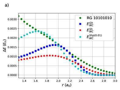
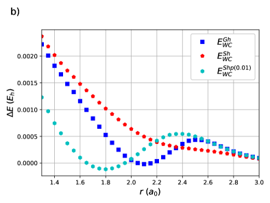
Figure 1: Weak correlation functionals for H₈ chain: (a) $|E_{WC}|$ compared with $\Delta_{RG}$. (b) Difference between $\Delta_{RG}$ and $|E_{WC}|$. 10101010 is the optimal RG state.

The best performing weak correlation functionals are $E^{Gh}_{WC}$ and $E^{Sh}_{WC}$, though $E^{Shp}_{WC}$ with a maximum at 0.01 is also reasonable. These results are shown in Figure 1. Functionals of the type (38) are always negative so their absolute values are plotted in Figure 1 to compare with $\Delta_{RG}$. The remaining error,

$$\Delta_{RG+WC}=E_{RG}+E_{WC}-E_{OO-DOCI}=\Delta_{RG}-|E_{WC}|$$ (53)

is plotted in Figure 1 (b). The other tested functionals either substantially over- or under-correlated (see supporting information). Of these three functionals, $E^{Sh}_{WC}$ appears to be the best behaved. All three under-correlate at short H–H distances. $E^{Shp(0.01)}_{WC}$ is the best at short H–H distances, but over-correlates at longer H–H separations, as does $E^{Gh}_{WC}$. $E^{Sh}_{WC}$ is the worst of the three at short H–H distances, but never over-correlates, has an error that decays monotonically, and is the best at longer H–H distances. All three functionals are reasonable given how they are essentially free to evaluate.

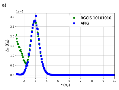
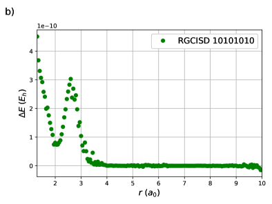
Figure 2: RGCIS and RGCISD treatment of H₈ chain: (a) $\Delta_{RGCIS}$ for the 10101010 RG state compared with similar results for APIG from ref.³⁴ (b) $\Delta_{RGCISD}$ for the 10101010 RG state. All results computed with the STO-6G basis set in the basis of OO-DOCI orbitals.

The RGCIS results in Figure 2 (a) seem to match the results obtained for APIG,³⁴

$$\ket{\text{APIG}}=\prod^{M}_{a=1}\sum^{N}_{i=1}G_{ai}S^{+}_{i}\ket{\theta}$$ (54)

for which the geminal coefficients $G_{ai}$ are variationally optimized. For HF Slater determinants, Brillouin’s theorem ensures that the optimal state does not couple with its CI singles. For RG states there is no Brillouin theorem, but the optimal state in terms of two-particle clusters would be APIG, which appears to be equivalent to RGCIS except at compressed geometries. The RGCISD results, in Figure 2 (b) are very close to DOCI. Occasionally RGCISD is found to be very slightly below DOCI, which must be attributed to loss of precision on the order of $10^{-12}$.

3.3 Paldus systems

In ref.⁹⁶ Paldus and co-workers presented four isomers of H₄, see Figure 3, that are multi-reference in terms of Slater determinants. S4 is a square of hydrogen atoms whose side length $\alpha$ is increased to the dissociated limit. P4 and D4 consist of two H₂ subunits with a fixed “bond-length” $a$ and a variable distance between subunits, $\alpha$. As $a$ is increased, the HOMO/LUMO pairs of each H₂ subunit get closer in energy, which increases the multi-reference character of the problem. Thus, following ref.,⁹⁶ three values of $a$ are considered: $a=1.2\;a_{0}$, $a=1.6\;a_{0}$, and $a=2.0\;a_{0}$. The quoted FCI value for the H₂ bond is $1.667\;a_{0}$, so these three choices represent a shortened bond-length, a near-equilibrium bond-length, and a stretched bond-length. H4 represents a square that opens to a line with fixed bond-lengths $a$. Again, the three values $a=1.2\;a_{0}$, $a=1.6\;a_{0}$, and $a=2.0\;a_{0}$ are considered.

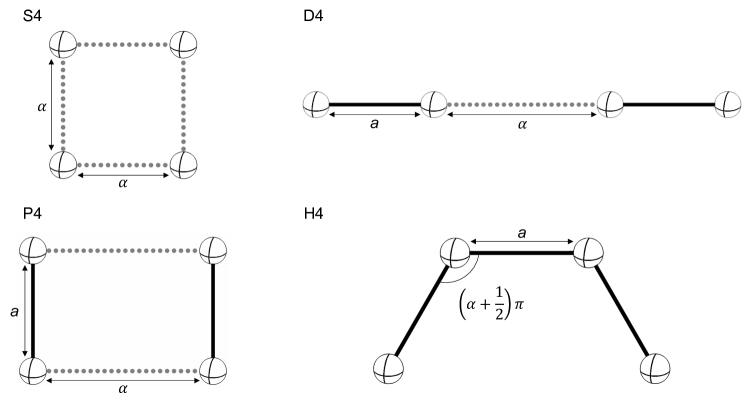
Figure 3: Paldus isomers of H₄. Solid lines have fixed length $a$ while dotted lines have variable length $\alpha$.

Figure 4 depicts FCI and OO-DOCI energies for S4 for a range of $\alpha=[1.0\;a_{0},8.0\;a_{0}]$. OO-DOCI provides near-quantitative accuracy with respect to FCI-derived energies. The maximum error in the OO-DOCI energy is only $\approx 0.014$ E${}_{\text{h}}$, around 2.8 $a_{0}$.

Figure 4: OO-DOCI treatment of Paldus S4: (a) FCI and OO-DOCI energies. (b) Error of OO-DOCI with respect to FCI. All results computed with the STO-6G basis set in the basis of OO-DOCI orbitals.

Variationally optimized 1010 RG states, shown in Figure 5, are energetically similar to OO-DOCI, never displaying more than 2 $\times 10^{-3}$ E${}_{\text{h}}$ error. Hence, the single RG state 1010 is similar to the OO-DOCI wavefunction throughout the potential energy curve. Figure 5 (b) shows that RGCIS built from the 1010 RG state is near-exact, with respect to OO-DOCI; maximum errors are only on the order of 10^-6 E${}_{\text{h}}$. Variational RG calculations were also performed for a 1100 RG state (see supporting information), but these states were found to be much too high in energy in the re-coupling region. Whereas for the 1010 RG state the $\{\varepsilon\}$ arrange themselves in a 2-2 pattern, for the 1100 RG state all the $\{\varepsilon\}$ are near-degenerate, which substantially increases the computational cost of solving the EBV equations (10). RGCISD results for the H₄ isomers are reported in the supporting information as the number of RG states included is the same as the number of Slater determinants in OO-DOCI. In these cases the RGCISD and OO-DOCI results agree on the order of $10^{-12}$.

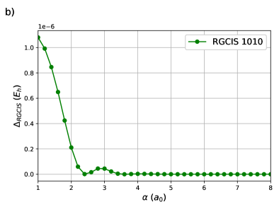
Figure 5: Variational RG and RGCI treatment of Paldus S4: (a) $\Delta_{RG}$ for the 1010 RG state. (b) $\Delta_{RGCIS}$ for the 1010 RG state. All results computed with the STO-6G basis set in the basis of OO-DOCI orbitals.

We also considered energy corrections from weak correlation functionals, applied to the 1010 RG reference, and the resulting data are shown in Figure 6. In general, we observe the same pattern as for linear H₈: the error for $E^{Gh}_{WC}$ has some oscillatory behavior while the error for $E^{Sh}_{WC}$ decays monotonically and should therefore be preferred.

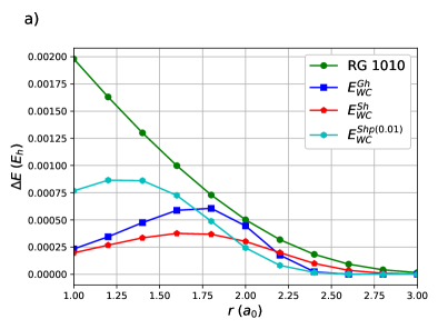
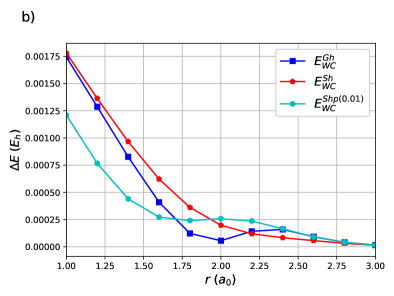
Figure 6: Weak correlation functionals for Paldus S4: (a) $|E_{WC}|$ compared with $\Delta_{RG}$. (b) Difference between $\Delta_{RG}$ and $|E_{WC}|$. 1010 is the optimal RG state. All results computed with the STO-6G basis set in the basis of OO-DOCI orbitals.

FCI and OO-DOCI results were computed for P4 with $a=1.2\;a_{0},1.6\;a_{0},2.0\;a_{0}$ for a range of $\alpha=[1.0\;a_{0},8.0\;a_{0}]$ and the results are presented in Figure 7. Generally OO-DOCI agrees with FCI, though there are visible gaps between the respective energies for both $a=1.6\;a_{0}$ and $a=2.0\;a_{0}$. This gap arises since the long and short sides of the rectangle switch, and hence the dominant Slater determinant the FCI expansion changes. Valence bonds form along the short sides of the rectangle, and for the square geometry two valence bond descriptions are degenerate.

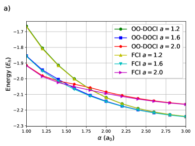
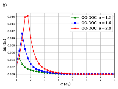
Figure 7: OO-DOCI treatment of Paldus P4 with $a=1.2\;a_{0},1.6\;a_{0},2.0\;a_{0}$: (a) FCI and OO-DOCI energies. Past $\alpha=3.0\;a_{0}$ the curves become indiscernible. (b) Error of OO-DOCI with respect to FCI. All results computed with the STO-6G basis set in the basis of OO-DOCI orbitals.

Figure 8 depicts deviations between energies from RG (1010) and RGCIS (built from 1010) states and the those from OO-DOCI. The correct RG state is 1010 for all values of $a$ and $\alpha$. The 1100 state was also variationally optimized, but it was found to have much too large an energy (see supporting information). RGCIS is near-exact, with errors with respect to OO-DOCI never exceeding $1.2\times 10^{-5}$ E${}_{\text{h}}$.

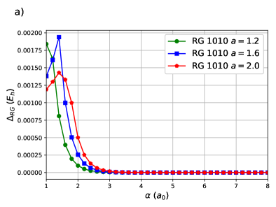
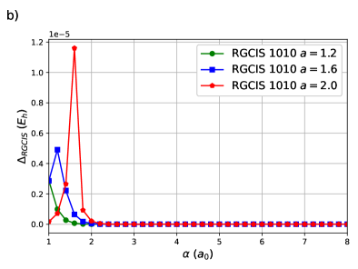
Figure 8: Variational RG and RGCI treatment of Paldus P4 with $a=1.2\;a_{0},1.6\;a_{0},2.0\;a_{0}$: (a) $\Delta_{RG}$ for the 1010 RG state. (b) $\Delta_{RGCIS}$ for the 1010 RG state. All results computed with the STO-6G basis set in the basis of OO-DOCI orbitals.

The weak correlation functionals do not provide any noticeable improvement upon the 1010 RG state (see supporting information). All of them under-correlate at small $\alpha$ and over-correlate at large $\alpha$.

FCI and OO-DOCI results were computed for D4 with $a=1.2\;a_{0},1.6\;a_{0},2.0\;a_{0}$ for a range of $\alpha=[1.0\;a_{0},8.0\;a_{0}]$ and the results are presented in Figure 9. The agreement between OO-DOCI and FCI is comparable to the case of P4, with maximum deviations between the methods being roughly twice as large ($\approx$ 0.03 E${}_{\text{h}}$ at 1.6 $a_{0}$) This gap occurs for a similar reason as for P4: when $\alpha<a$, the bonding pattern should be centred between the second and third hydrogen atoms as they are closest. Contributions from the seniority two and four sectors are required for quantitative agreement with FCI.

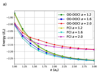
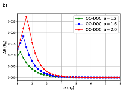
Figure 9: OO-DOCI treatment of Paldus D4 with $a=1.2\;a_{0},1.6\;a_{0},2.0\;a_{0}$: (a) FCI and OO-DOCI energies. (b) Error of OO-DOCI with respect to FCI. All results computed with the STO-6G basis set in the basis of OO-DOCI orbitals.

Variational RG calculations capture the transition in the bonding pattern explicitly. When $\alpha<a$, the correct RG state is 1100 with a set of $\{\varepsilon\}$ arranged in a 1-2-1 energetic pattern: 1 small $\varepsilon$, 2 near-degenerate $\varepsilon$, and 1 large $\varepsilon$. This arrangement corresponds to one doubly-occupied orbital, two partially-occupied valence orbitals, and one empty virtual orbital. Once $\alpha\geq a$, the correct RG state is 1010 with a set of $\{\varepsilon\}$ in two sets of near-degenerate pairs. With the correct RG reference, the RGCIS results never differ from OO-DOCI by more than $2\times 10^{-6}E_{\text{h}}$.

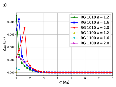
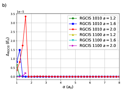
Figure 10: Variational RG and RGCI treatment of Paldus D4 with $a=1.2\;a_{0},1.6\;a_{0},2.0\;a_{0}$: (a) $\Delta_{RG}$ for the 1010 and 1100 RG states. (b) $\Delta_{RGCIS}$ for the 1010 and 1100 RG states. 1100 is only optimal at short distances and quickly jumps off the scale once $\alpha>a$. All results computed with the STO-6G basis set in the basis of OO-DOCI orbitals.

As was the case for P4, the weak-correlation functionals do not provide any useful improvement (see supporting information). At short distances they all under-correlate substantially and at long distances they all over-correlate substantially.

Figure 11 depicts FCI and OO-DOCI potential energy curves for the H4 model with $a=1.2\;a_{0},1.6\;a_{0},2.0\;a_{0}$. The OO-DOCI and FCI curves are qualitatively similar though the agreement is not quantitative, which indicates the need for weak correlation contributions from higher seniority sectors.

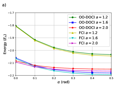
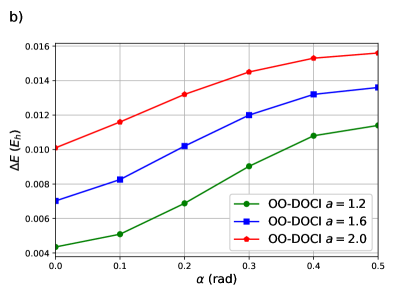
Figure 11: OO-DOCI treatment of Paldus H4 with $a=1.2\;a_{0},1.6\;a_{0},2.0\;a_{0}$: (a) FCI and OO-DOCI energies. (b) Error of OO-DOCI with respect to FCI. All results computed with the STO-6G basis set in the basis of OO-DOCI orbitals.

Variational RG calculations, presented in Figure 12, show that a 1010 RG state recovers OO-DOCI energies to within roughly 1.6 $\times 10^{-3}$ E${}_{\text{h}}$ throughout the curve, and several orders of magnitude of improvement can be obtained with RGCIS.

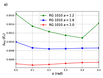
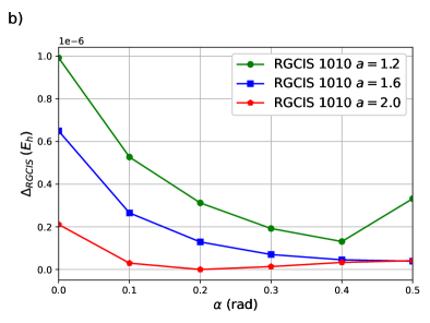
Figure 12: Variational RG and RGCI treatment of H4 with $a=1.2\;a_{0},1.6\;a_{0},2.0\;a_{0}$: (a) $\Delta_{RG}$ for the 1010 RG state. (b) $\Delta_{RGCIS}$ for the 1010 RG state. All results computed with the STO-6G basis set in the basis of OO-DOCI orbitals.

In this case, the relative performance of the weak correlation functionals is less clear: for each choice of $a$, a different functional was found to be optimal (Figure 13). At $a=1.2\;a_{0}$ $E^{Ghp}_{WC}$ performs the best, at $a=1.6\;a_{0}$ $E^{Shp}_{WC}$ with a maximum at 0.01 is best, while at $a=2.0\;a_{0}$ the best performing functional is $E^{Gh}_{WC}$. Results for all eight tested functionals are included in the supporting information.

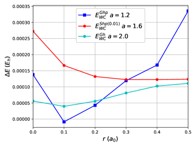
Figure 13: Weak correlation functionals for Paldus H4 with $a=1.2\;a_{0},1.6\;a_{0},2.0\;a_{0}$: Difference between $\Delta_{RG}$ and $|E_{WC}|$. 1010 is the optimal RG state. All results computed with the STO-6G basis set in the basis of OO-DOCI orbitals.

3.4 H₁₀ isomers

Recently, Stair and Evangelista presented four isomers of H₁₀, shown in Figure 14, to assess not only the accuracy of some common quantum chemistry approaches, but also their ability to provide compact representations of the electronic structure of these complex systems. Each isomer can be thought of as a proxy for a finite-size Hubbard model: the single variable is the inter-atomic distance which modulates on-site repulsion. The chain and the ring are similar to 1-dimensional Hubbard models without and with periodic boundary conditions, respectively. In the sheet system, the hydrogen atoms are arranged in a 3-4-3 pattern, with all of the nearest-neighbours being equidistant. The pyramid is a tetrahedron with four hydrogen atoms at the vertices and the six remaining hydrogen atoms at the midpoint of each of the edges.

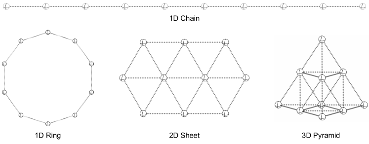
Figure 14: Isomers of H₁₀ considered in this work. The dashed lines are of equivalent distance.

Figure 15 depicts potential energy curves for the four H₁₀ isomers computed at the OO-DOCI / STO-6G level of theory. FCI results computed the same basis, which were taken from Ref.,⁹⁷ are also provided. As expected, OO-DOCI does a reasonable job of reproducing the overall shapes of the FCI curves for both of the 1D structures. As can be seen in Fig. 16, the maximum deviations between OO-DOCI and FCI are $\approx 0.67$ E${}_{\text{h}}$ and $\approx 0.97$ E${}_{\text{h}}$ for the 1D chain and ring structures respectively. For the 2D and 3D structures, the largest deviations between OO-DOCI and FCI energies are somewhat larger; moreover, for these systems, we also begin to see some qualitative differences in the shapes of the respective curves. For the 2D sheet, the curvature at intermediate H–H distances is different than that from FCI. For the 3D pyramid, OO-DOCI predicts only a shallow minimum at roughly the correct H–H distance, after which it exhibits a small hump before it appears to approach the correct dissociation limit. Even so, when considering additional correlation treatments, OO-DOCI should be a much better starting point than restricted Hartree-Fock (RHF). We now show that OO-DOCI can itself be very well approximated by a single RG state in all cases.

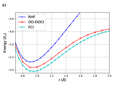
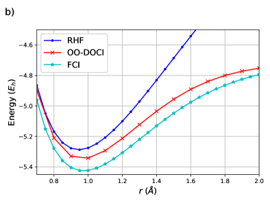
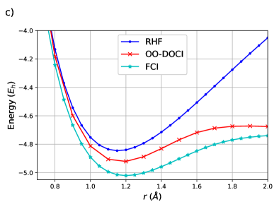
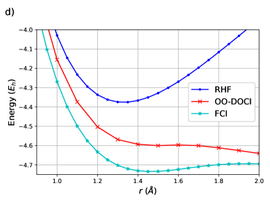
Figure 15: OO-DOCI treatment of H₁₀ isomers: RHF, OO-DOCI and FCI energies for (a) 1-dimensional chain. (b) 1-dimensional ring. (c) 2-dimensional sheet. (d) 3-dimensional pyramid. OO-DOCI results computed with the STO-6G basis set in the basis of OO-DOCI orbitals. RHF and FCI results are from ref.⁹⁷

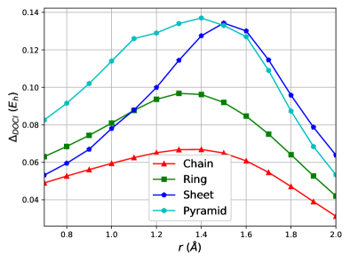
Figure 16: OO-DOCI error with respect to FCI for H₁₀ isomers. All results computed with the STO-6G basis set in the basis of OO-DOCI orbitals.

3.4.1 1D structures

The linear chain is exactly the same as those we have already studied, except that the chain is one GVB pair longer. Hence, the optimal RG state is the Néel RG state (1010101010). The error in the RG energy with respect to that from OO-DOCI is shown in Figure 17 (a). The maximum deviation from the OO-DOCI energy ($\approx$4 $\times 10^{-3}$ E${}_{\text{h}}$) occurs at the most compressed geometry considered, and the RG state effectively recovers the OO-DOCI energy at stretched geometries. As seen in Fig. 17 (b), the additional correlation provided by RGCIS brings the error with respect to OO-DOCI down several orders of magnitude in the equilibrium region. The errors in the RGCIS energy are all less than 4 $\times 10^{-6}$ E${}_{\text{h}}$ throughout the entire curve. To the precision we can trust our results, RGCISD is essentially indiscernible from OO-DOCI (see supporting information).

The ring is a finite size “periodic” 1D structure. We expect that the relative performance of RG and OO-DOCI should be of similar quality to the case of the chain structure, and, indeeed, it is: the optimal RG state is the Néel RG state and the error in its energy with respect to OO-DOCI, shown in Figure 17 (a), is only slightly larger than for the chain at compressed geometries and quite similar at stretched geometries. Again, the additional correlation afforded by RGCIS brings the error down by several orders of magnitude (Fig. 17 (b)).

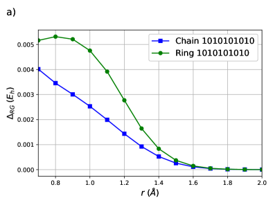
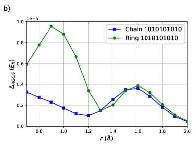
Figure 17: Variational RG and RGCIS treatment of H₁₀ chain and ring: (a) $\Delta_{RG}$ for the 1010101010 RG state. (b) $\Delta_{RGCIS}$ for the 1010101010 RG state. All results computed with the STO-6G basis set in the basis of OO-DOCI orbitals.

Corrections from the weak correlation functionals, shown in Figure 18, follow the same pattern as for linear H₈: $E^{Gh}_{WC}$ and $E^{Sh}_{WC}$ are both reasonable, though $E^{Sh}_{WC}$ should be preferred as it never over-correlates and its error with respect to OO-DOCI decays monotonically.

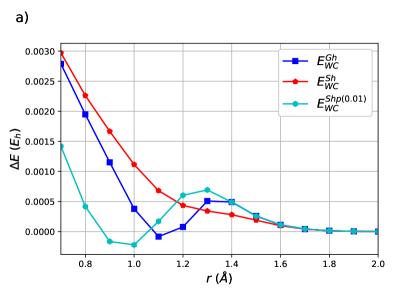
Figure 18: Weak correlation functionals for 1D H₁₀ isomers: (a) Difference between $\Delta_{RG}$ and $|E_{WC}|$ for 1D chain. (b) Difference between $\Delta_{RG}$ and $|E_{WC}|$ for 1D ring. 1010101010 is the optimal RG state. All results computed with the STO-6G basis set in the basis of OO-DOCI orbitals.

3.4.2 Sheet and pyramid

The sheet is the first case where there is an appreciable qualitative difference between OO-DOCI and FCI. We also found that the optimal variational RG states change in this case. As can be seen in Fig. 19 (a), the Néel RG state is optimal everywhere except at compressed geometries.

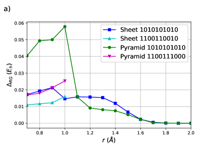
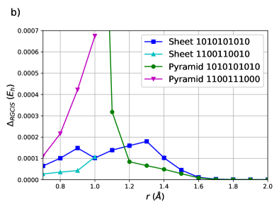
Figure 19: Variational RG and RGCIS treatment of H₁₀ sheet and pyramid: (a) $\Delta_{RG}$ for the 1010101010, 1100110010 (sheet) and 1100111000 (pyramid) RG states. (b) $\Delta_{RGCIS}$ for the 1010101010, 1100110010 (sheet) and 1100111000 (pyramid) RG states. Past 1.1, the curves for 1100110010 (sheet) and 1100111000 (pyramid) jump off the graph. All results computed with the STO-6G basis set in the basis of OO-DOCI orbitals.

For H–H distances less than or equal to 1.0 Å, we found that the optimal RG state is instead 1100110010, for which the single-particle energies $\{\varepsilon\}$ arrange themselves in a 4-4-2 pattern: there are 4 orbitals that contain 2 pairs, another 4 orbitals that contain another 2 pairs, and 2 orbitals that contain 1 pair. This structure is perhaps more clear from the corresponding geminal coefficient matrix

$$G_{ai}=\frac{1}{u_{a}-\varepsilon_{i}}\approx\begin{pmatrix}*&*&*&*&0&0&0&0&0&0\\ *&*&*&*&0&0&0&0&0&0\\ 0&0&0&0&*&*&*&*&0&0\\ 0&0&0&0&*&*&*&*&0&0\\ 0&0&0&0&0&0&0&0&*&*\end{pmatrix}$$ (55)

which is block diagonal. Again, the elements in the off-diagonal blocks are not numerically zero, but they are much smaller than those in the diagonal blocks. Remarkably, this state does not seem to be describable as GVB/APSG, for which the matrix $G_{ai}$ is (15), nor AP1roG/pCCD, for which $G_{ai}$ is

$$G_{ai}=\begin{pmatrix}1&0&0&0&0&*&*&*&*&*\\ 0&1&0&0&0&*&*&*&*&*\\ 0&0&1&0&0&*&*&*&*&*\\ 0&0&0&1&0&*&*&*&*&*\\ 0&0&0&0&1&*&*&*&*&*\end{pmatrix}.$$ (56)

For GVB/APSG and AP1roG/pCCD, the elements marked “0” in $G_{ai}$ are identically zero.

As for the 1D chain and ring structures, RGCIS improves upon the single, optimal RG state, decreasing the energy error by several orders of magnitude (Fig. 19 (b)). However, in this case, the RGCIS error is somewhat larger at compressed geometries. The maximum error is $\approx 2\times 10^{-4}$ E${}_{\text{h}}$, at an H–H distance of 1.3 Å, but this error decreases rapidly (as does that for the single RG state) at larger H–H distances. RGCISD, with the correct RG reference, has a maximum error of $\approx 1\times 10^{-6}$ E${}_{\text{h}}$ at 1.3 Å  (see supporting information).

Variational RG minimization for the 3D pyramid, shown in Figure 19 (a), again found the Néel RG state to be optimal, except at short H–H distances where the optimal RG state found was 1100111000. In this case, the single-particle energies $\{\varepsilon\}$ arrange themselves in a 4-6 pattern: there are 4 sites that contain 2 pairs and 6 sites that contain the remaining 3. The corresponding geminal coefficient matrix has the form

$$G_{ai}=\frac{1}{u_{a}-\varepsilon_{i}}\approx\begin{pmatrix}*&*&*&*&0&0&0&0&0&0\\ *&*&*&*&0&0&0&0&0&0\\ 0&0&0&0&*&*&*&*&*&*\\ 0&0&0&0&*&*&*&*&*&*\\ 0&0&0&0&*&*&*&*&*&*\end{pmatrix}.$$ (57)

Again, the elements labelled “0” are not numerically zero, but they are much smaller than those labelled “*”. This state also does not appear to be describable as GVB/APSG nor AP1roG/pCCD. As seen in the other systems, the energies obtained from RGCIS improve significantly upon those from a single RG state, although the RGCIS error is somewhat larger for the pyramid than for the sheet at short H–H distances. Nonetheless, the RGCIS error never exceeds $7\times 10^{-4}$ E${}_{\text{h}}$, and the error decreases rapidly (as does that for the single RG state) at larger distances. RGCISD, with the correct RG reference, has a maximum error of $\approx 3\times 10^{-6}$ E${}_{\text{h}}$ at 1.0 Å(see supporting information).

The best performing weak correlation functionals, shown in Figure 20, are different than for the 1D structures. $E^{Ghp}_{WC}$ and $E^{Shp}_{WC}$ are now the best for both the 2D sheet and the 3D pyramid. $E^{Shp}_{WC}$ should be preferred as its error with respect to OO-DOCI is much better behaved.

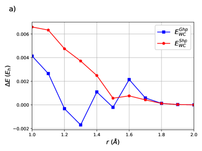
Figure 20: Weak correlation functionals for H₁₀ sheet and pyramid: (a) Differences between $\Delta_{RG}$ and $|E_{WC}|$ for 2D sheet. (b) Differences between $\Delta_{RG}$ and $|E_{WC}|$ for 3D pyramid. Results are only computed for the region where 1010101010 is the optimal RG state. All results computed with the STO-6G basis set in the basis of OO-DOCI orbitals.

A discussion of the correct choice of RG state is warranted. Given that there are $\binom{10}{5}$ possible RG states for 5 pairs in 10 orbitals, how can we be sure we have the correct one? With a few observations we can reduce this number to one that is completely manageable. First, we have observed that the single-particle energies $\{\varepsilon\}$ tend to separate into partitions of $2k$ elements for $k$ pairs. Second, within a partition we always want the 1s listed first, as otherwise the pairs will be placed principally in higher energy orbitals which leads to much higher energies. Third, the order of the partitions in a bitstring does not matter, e.g. the bitstrings 1100111000 and 1110001100 refer to different RG states for a given set of $\{\varepsilon\}$ and $g$, but when optimized will find equivalent solutions. In this contribution we found results for 1100111000 first. Thus, the only RG states that must be considered are in one-to-one correspondence with the partitions of the number of pairs:

$$(5) \mapsto 1111100000$$

$$(4,1) \mapsto 11110000\;10$$

$$(3,2) \mapsto 111000\;1100$$

$$(3,1,1) \mapsto 111000\;10\;10$$

$$(2,2,1) \mapsto 1100\;1100\;10$$

$$(2,1,1,1) \mapsto 1100\;10\;10\;10$$

$$(1,1,1,1,1) \mapsto 10\;10\;10\;10\;10.$$ (58)

Finally, symmetry arguments can reduce this list to a few possible candidates. In the pyramid, the four vertices are equivalent and the six edges are equivalent, so it is not surprising that 1100111000 is the optimal RG state at short distances. In the sheet, the two inner hydrogen atoms are equivalent and the four corners are equivalent. It is not obvious whether the other four hydrogen atoms are equivalent or not, and, thus it is necessary to try all bitstrings containing partitions (2,1). These rules are meant to rationalize our results. In this study many more possible RG states were tested, but none fell outside of these observations. These arguments notwithstanding, our experience is that, at large H–H separations distances, the Néel RG state is always optimal.

4 Conclusion

We have computed OO-DOCI wavefunctions and RG states for hydrogen clusters containing four, eight, and ten hydrogen atoms. With the exception of the pyramid structure for H₁₀, OO-DOCI captures the correct qualitative behavior of the energy as a function of H–H distance in all cases. OO-DOCI itself has been shown to be well approximated by a single RG state, while RGCIS significantly improves this approximation. RGCISD states are effectively indiscernible from OO-DOCI states, in terms of the energy. Hence, when the electronic structure of these systems is represented in terms of RG states, rather than Slater determinants, these systems all appear to be effectively single-reference. Given the good performance of RGCIS and RGCISD, it is worth pursuing improved expressions of the TDM elements, as the expressions reported herein are expensive to evaluate but are certainly improvable.

As an alternative to RGCIS or RGCISD, we explored the utility of weak correlation functionals within the seniority-zero channel, which are computationally inexpensive to evaluate. For 1D structures we found that the best performance was obtained for the $E^{Sh}_{WC}$ functional, while for 2D and 3D structures we best-performing functional was $E^{Shp}_{WC}$. In general, the Slater type functionals we considered are to be preferred over Gaussian type as their error with respect to OO-DOCI is better behaved. The exception is the Paldus ring-opening system (H4) for which $E^{Ghp}_{WC}$ was the best for $a=1.2a_{0}$ while $E^{Gh}_{WC}$ was the best at longer bond lengths.

Regardless of the route chosen to recover the full energy within the seniority-zero sector, quantitative agreement with FCI will ultimately require contributions from the seniority-two and seniority-four channels. Such contributions can be included post-hoc in a number of ways.^{57, 73, 80, 125, 126}

Finally, we reiterate that the optimal RG state for the H₁₀ isomers is the Néel state except for the 2D sheet and the 3D pyramid at short distances. There, the single particle energies $\{\varepsilon\}$ arrange into larger clusters that accommodate more than one pair. This behavior is not allowed by the geminal coefficients of GVB/APSG, nor AP1roG/pCCD.

The authors thank Mario Piris and Alexandre Faribault for helpful discussions. P.A.J. was supported by NSERC and the Digital Research Alliance of Canada. A.E.D. acknowledges support from the National Science Foundation under Grant No. OAC-2103705.

References

- Čížek 1966 Čížek, J. The Journal of Chemical Physics 1966, 45, 4256–4266
- Čížek and Paldus 1971 Čížek, J.; Paldus, J. International Journal of Quantum Chemistry 1971, 5, 359–379
- Shavitt and Bartlett 2009 Shavitt, I.; Bartlett, R. J. Many-Body Methods in Chemistry and Physics; Cambridge University Press: Cambridge, 2009
- Bartlett and Musiał 2007 Bartlett, R. J.; Musiał, M. Reviews of Modern Physics 2007, 79, 291–352
- Purvis III and Bartlett 1982 Purvis III, G. D.; Bartlett, R. J. The Journal of Chemical Physics 1982, 76, 1910–1918
- Roos et al. 1980 Roos, B. O.; Taylor, P. R.; Siegbahn, P. E. M. Chemical Physics 1980, 48, 157–173
- Siegbahn et al. 1980 Siegbahn, P. E. M.; Heiberg, A.; Roos, B.; Levy, B. Physica Scripta 1980, 21, 323–327
- Siegbahn et al. 1981 Siegbahn, P. E. M.; Almlöf, J.; Heiberg, A.; Roos, B. The Journal of Chemical Physics 1981, 74, 2384–2396
- Roos 1987 Roos, B. O. Advances in Chemical Physics; John Wiley & Sons, Ltd, 1987; pp 399–445
- Vogiatzis et al. 2017 Vogiatzis, K. D.; Ma, D.; Olsen, J.; Gagliardi, L.; de Jong, W. A. The Journal of Chemical Physics 2017, 147, 184111
- Olsen et al. 1988 Olsen, J.; Roos, B. J.; Jørgenson, P.; Jensen, H. J. A. The Journal of Chemical Physics 1988, 89, 2185–2192
- Malmqvist et al. 1990 Malmqvist, P. A.; Rendell, A.; Roos, B. O. The Journal of Physical Chemistry 1990, 94, 5477–5482
- Fleig et al. 2001 Fleig, T.; Olsen, J.; Marian, C. M. The Journal of Chemical Physics 2001, 114, 4775–4790
- Ma et al. 2011 Ma, D.; Manni, G. L.; Gagliardi, L. The Journal of Chemical Physics 2011, 135, 044128
- Manni et al. 2013 Manni, G. L.; Ma, D.; Aquilante, F.; Olsen, J.; Gagliardi, L. Journal of Chemical Theory and Computation 2013, 9, 3375–3384
- Thomas et al. 2015 Thomas, R. E.; Sun, Q.; Alavi, A.; Booth, G. H. Journal of Chemical Theory and Computation 2015, 11, 5316–5325
- Manni et al. 2016 Manni, G. L.; Smart, S. D.; Alavi, A. Journal of Chemical Theory and Computation 2016, 12, 1245–1258
- Schriber and Evangelista 2016 Schriber, J. B.; Evangelista, F. A. The Journal of Chemical Physics 2016, 144, 161106
- Levine et al. 2020 Levine, D. S.; Hait, D.; Tubman, N. M.; Lehtola, S.; Whaley, K. B.; Head-Gordon, M. Journal of Chemical Theory and Computation 2020, 16, 2340–2354
- Ghosh et al. 2008 Ghosh, D.; Hachmann, J.; Yanai, T.; Chan, G. K.-L. The Journal of Chemical Physics 2008, 128, 144117
- Yanai et al. 2009 Yanai, T.; Kurashige, Y.; Ghosh, D.; Chan, G. K.-L. International Journal of Quantum Chemistry 2009, 109, 2178–2190
- Wouters et al. 2014 Wouters, S.; Poelmans, W.; Ayers, P. W.; Van Neck, D. Computer Physics Communications 2014, 185, 1501–1514
- Sun et al. 2017 Sun, Q.; Yang, J.; Chan, G. K.-L. Chemical Physics Letters 2017, 683, 291–299
- Ma et al. 2017 Ma, Y.; Knecht, S.; Keller, S.; Reiher, M. Journal of Chemical Theory and Computation 2017, 13, 2533–2549
- Gidofalvi and Mazziotti 2008 Gidofalvi, G.; Mazziotti, D. A. The Journal of Chemical Physics 2008, 129, 134108
- Fosso-Tande et al. 2016 Fosso-Tande, J.; Nguyen, T.-S.; Gidofalvi, G.; DePrince III, A. E. Journal of Chemical Theory and Computation 2016, 12, 2260–2271
- Fock 1950 Fock, V. Doklady Akademii Nauk SSSR 1950, 73, 735–739
- Silver 1969 Silver, D. M. The Journal of Chemical Physics 1969, 50, 5108–5116
- Silver 1970 Silver, D. M. The Journal of Chemical Physics 1970, 52, 299–303
- Silver et al. 1970 Silver, D. M.; Mehler, E. L.; Ruedenberg, K. The Journal of Chemical Physics 1970, 52, 1174–1180
- Silver et al. 1970 Silver, D. M.; Ruedenberg, K.; Mehler, E. L. The Journal of Chemical Physics 1970, 52, 1206–1227
- Paldus 1972 Paldus, J. The Journal of Chemical Physics 1972, 57, 638–651
- Paldus et al. 1972 Paldus, J.; Sengupta, S.; Čížek, J. The Journal of Chemical Physics 1972, 57, 652–666
- Moisset et al. 2022 Moisset, J.-D.; Fecteau, C.-E.; Johnson, P. A. The Journal of Chemical Physics 2022, 156, 214110
- Bardeen et al. 1957 Bardeen, J.; Cooper, L. N.; Schrieffer, J. R. Physical Review 1957, 106, 162–164
- Bardeen et al. 1957 Bardeen, J.; Cooper, L. N.; Schrieffer, J. R. Physical Review 1957, 108, 1175–1204
- Schrieffer 1964 Schrieffer, J. R. Theory of Superconductivity; CRC Press: Boca Raton, 1964
- Coleman 1965 Coleman, A. J. Journal of Mathematical Physics 1965, 6, 1425–1431
- Ortiz et al. 1981 Ortiz, J. V.; Weiner, B.; Öhrn, Y. International Journal of Quantum Chemistry 1981, 20, 113–128
- Sarma et al. 1989 Sarma, C. R.; Paldus, J.; Öhrn, Y. International Journal of Quantum Chemistry 1989, 36, 35–48
- Coleman 1997 Coleman, A. J. International Journal of Quantum Chemistry 1997, 63, 23–30
- Henderson and Scuseria 2019 Henderson, T. M.; Scuseria, G. E. The Journal of Chemical Physics 2019, 151, 051101
- Khamoshi et al. 2019 Khamoshi, A.; Henderson, T. M.; Scuseria, G. E. The Journal of Chemical Physics 2019, 151, 184103
- Dutta et al. 2020 Dutta, R.; Henderson, T. M.; Scuseria, G. E. Journal of Chemical Theory and Computation 2020, 16, 6358–6367
- Khamoshi et al. 2021 Khamoshi, A.; Chen, G. P.; Henderson, T. M.; Scuseria, G. E. The Journal of Chemical Physics 2021, 154, 074113
- Dutta et al. 2021 Dutta, R.; Chen, G. P.; Henderson, T. M.; Scuseria, G. E. The Journal of Chemical Physics 2021, 154, 114112
- Neuscamman 2012 Neuscamman, E. Physical Review Letters 2012, 109, 203001
- Neuscamman 2013 Neuscamman, E. The Journal of Chemical Physics 2013, 139, 194105
- Neuscamman 2016 Neuscamman, E. Molecular Physics 2016, 114, 577–583
- Hurley et al. 1953 Hurley, A. C.; Lennard-Jones, J. E.; Pople, J. A. Proceedings of the Royal Society 1953, A220, 446–455
- Kutzelnigg 1964 Kutzelnigg, W. The Journal of Chemical Physics 1964, 40, 3640–3647
- Goddard III 1967 Goddard III, W. A. Physical Review 1967, 157, 81
- Hay et al. 1972 Hay, P. J.; Hunt, W. J.; Goddard III, W. A. Chemical Physics Letters 1972, 13, 30–35
- Hunt et al. 1972 Hunt, W. J.; Hay, P. J.; Goddard III, W. A. The Journal of Chemical Physics 1972, 57, 738–748
- Goddard III et al. 1973 Goddard III, W. A.; Dunning, T. H.; Hunt, W. J.; Hay, P. J. Accounts of Chemical Research 1973, 6, 368–376
- Kutzelnigg 2010 Kutzelnigg, W. In Recent Progress in Coupled Cluster Methods: Theory and Applications; Cársky, P., Paldus, J., Pittner, J., Eds.; Springer Netherlands: Dordrecht, 2010; pp 299–356
- Kobayashi et al. 2010 Kobayashi, M.; Szabados, A.; Nakai, H.; Surjan, P. Journal of Chemical Theory and Computation 2010, 6, 2024–2033
- Kutzelnigg 2012 Kutzelnigg, W. Chemical Physics 2012, 401, 119–124
- Surján et al. 2012 Surján, P. R.; Szabados, A.; Jeszenski, P.; Zoboki, T. Journal of Mathematical Chemistry 2012, 50, 534–551
- Zoboki et al. 2013 Zoboki, T.; Szabados, A.; Surján, P. R. Journal of Chemical Theory and Computation 2013, 9, 2602–2608
- Pernal 2014 Pernal, K. Journal of Chemical Theory and Computation 2014, 10, 4332–4341
- Jeszenszki et al. 2014 Jeszenszki, P.; Nagy, P. R.; Zoboki, T.; Szabados, A.; Surján, P. R. International Journal of Quantum Chemistry 2014, 114, 1048–1052
- Pastorczak and Pernal 2015 Pastorczak, E.; Pernal, K. Physical Chemistry Chemical Physics 2015, 17, 8622–8626
- Margócsy et al. 2018 Margócsy, A.; Kowalski, P.; Pernal, K.; Szabados, A. Theoretical Chemistry Accounts 2018, 137, 1–3
- Pernal 2018 Pernal, K. The Journal of Chemical Physics 2018, 149, 204101
- Pastorczak and Pernal 2018 Pastorczak, E.; Pernal, K. Theoretical Chemistry Accounts 2018, 137, 1–10
- Pastorczak et al. 2019 Pastorczak, E.; Jensen, H. J. A.; Kowalski, P. H.; Pernal, K. Journal of Chemical Theory and Computation 2019, 15, 4430–4439
- Piris et al. 2011 Piris, M.; Lopez, X.; Ruipérez, F.; Matxain, J. M.; Ugalde, J. M. The Journal of Chemical Physics 2011, 134, 164102
- Wang et al. 2019 Wang, Q.; Zou, J.; Xu, E.; Pulay, P.; S., L. Journal of Chemical Theory and Computation 2019, 15, 141–153
- Limacher et al. 2013 Limacher, P. A.; Ayers, P. W.; Johnson, P. A.; De Baerdemacker, S.; Van Neck, D.; Bultinck, P. Journal of Chemical Theory and Computation 2013, 9, 1394–1401
- Stein et al. 2014 Stein, T.; Henderson, T. M.; Scuseria, G. E. The Journal of Chemical Physics 2014, 140, 214113
- Limacher et al. 2014 Limacher, P. A.; Kim, T. D.; Ayers, P. W.; Johnson, P. A.; De Baerdemacker, S.; Van Neck, D.; Bultinck, P. Molecular Physics 2014, 112, 853–862
- Limacher et al. 2014 Limacher, P. A.; Ayers, P. W.; Johnson, P. A.; De Baerdemacker, S.; Van Neck, D.; Bultinck, P. Physical Chemistry Chemical Physics 2014, 16, 5061–5065
- Henderson et al. 2014 Henderson, T. M.; Scuseria, G. E.; Dukelsky, J.; Signoracci, A.; Duguet, T. Physical Review C 2014, 89, 054305
- Henderson et al. 2014 Henderson, T. M.; Bulik, I. W.; Stein, T.; Scuseria, G. E. The Journal of Chemical Physics 2014, 141, 244104
- Boguslawski et al. 2014 Boguslawski, K.; Tecmer, P.; Ayers, P. W.; Bultinck, P.; De Baerdemacker, S.; Van Neck, D. Physical Review B 2014, 89, 201106(R)
- Boguslawski et al. 2014 Boguslawski, K.; Tecmer, P.; Bultinck, P.; De Baerdemacker, S.; Van Neck, D.; Ayers, P. W. Journal of Chemical Theory and Computation 2014, 10, 4873–4882
- Boguslawski et al. 2014 Boguslawski, K.; Tecmer, P.; Limacher, P. A.; Johnson, P. A.; Ayers, P. W.; Bultinck, P.; De Baerdemacker, S.; Van Neck, D. The Journal of Chemical Physics 2014, 140, 214114
- Tecmer et al. 2014 Tecmer, P.; Boguslawski, K.; Johnson, P. A.; Limacher, P. A.; Chan, M.; Verstraelen, T.; Ayers, P. W. Journal of Physical Chemistry 2014, A118, 9058–9068
- Boguslawski and Ayers 2015 Boguslawski, K.; Ayers, P. W. Journal of Chemical Theory and Computation 2015, 11, 5252–5261
- Boguslawski et al. 2016 Boguslawski, K.; Tecmer, P.; Legeza, O. Physical Review B 2016, 94, 155126
- Boguslawski 2016 Boguslawski, K. The Journal of Chemical Physics 2016, 145, 234105
- Boguslawski and Tecmer 2017 Boguslawski, K.; Tecmer, P. Journal of Chemical Theory and Computation 2017, 13, 5966–5983
- Boguslawski 2019 Boguslawski, K. Journal of Chemical Theory and Computation 2019, 15, 18–24
- Nowak et al. 2019 Nowak, A.; Tecmer, P.; Boguslawski, K. Physical Chemistry Chemical Physics 2019, 21, 19039–19053
- Boguslawski 2021 Boguslawski, K. Chemical Communications 2021, 57, 12277–12280
- Nowak et al. 2021 Nowak, A.; Legeza, O.; Boguslawski, K. The Journal of Chemical Physics 2021, 154, 084111
- Marie et al. 2021 Marie, A.; Kossoski, F.; Loos, P.-F. The Journal of Chemical Physics 2021, 155, 104105
- Kossoski et al. 2021 Kossoski, F.; Marie, A.; Scemama, A.; Caffarel, M.; Loos, P.-F. Journal of Chemical Theory and Computation 2021, 17, 4756–4768
- Richardson 1963 Richardson, R. W. Physics Letters 1963, 3, 277–279
- Richardson and Sherman 1964 Richardson, R. W.; Sherman, N. Nuclear Physics 1964, 52, 221–238
- Richardson 1965 Richardson, R. W. Journal of Mathematical Physics 1965, 6, 1034–1051
- Gaudin 1976 Gaudin, M. Journal de Physique 1976, 37, 1087–1098
- Johnson et al. 2020 Johnson, P. A.; Fecteau, C.-E.; Berthiaume, F.; Cloutier, S.; Carrier, L.; Gratton, M.; Bultinck, P.; De Baerdemacker, S.; Van Neck, D.; Limacher, P.; Ayers, P. W. The Journal of Chemical Physics 2020, 153, 104110
- Fecteau et al. 2022 Fecteau, C.-E.; Cloutier, S.; Moisset, J.-D.; Boulay, J.; Bultinck, P.; Faribault, A.; Johnson, P. A. The Journal of Chemical Physics 2022, 156, 194103
- Paldus et al. 1993 Paldus, J.; Piecuch, P.; Pylypow, L.; Jeziorski, B. Physical Review A 1993, 47, 2738–2782
- Stair and Evangelista 2020 Stair, N. H.; Evangelista, F. A. The Journal of Chemical Physics 2020, 153, 104108
- Gorohovsky and Bettelheim 2011 Gorohovsky, G.; Bettelheim, E. Physical Review B 2011, 84, 224503
- Fecteau et al. 2020 Fecteau, C.-E.; Fortin, H.; Cloutier, S.; Johnson, P. A. The Journal of Chemical Physics 2020, 153, 164117
- Johnson et al. 2021 Johnson, P. A.; Fortin, H.; Cloutier, S.; Fecteau, C.-E. The Journal of Chemical Physics 2021, 154, 124125
- Fecteau et al. 2021 Fecteau, C.-E.; Berthiaume, F.; Khalfoun, M.; Johnson, P. A. Journal of Mathematical Chemistry 2021, 59, 289–301
- Faribault et al. 2022 Faribault, A.; Dimo, C.; Moisset, J.-D.; Johnson, P. A. The Journal of Chemical Physics 2022, 157, 214104
- Rombouts et al. 2004 Rombouts, S.; Van Neck, D.; Dukelsky, J. Physical Review C 2004, 69, 061303(R)
- Guan et al. 2012 Guan, X.; Launey, K. D.; Xie, M.; Bao, L.; Pan, F.; Draayer, J. P. Physical Review C 2012, 86, 024313
- Pogosov 2012 Pogosov, W. V. Journal of Physics: Condensed Matter 2012, 24, 075701
- De Baerdemacker 2012 De Baerdemacker, S. Physical Review C 2012, 86, 044332
- Faribault et al. 2011 Faribault, A.; El Araby, O.; Sträter, C.; Gritsev, V. Physical Review B 2011, 83, 235124
- El Araby et al. 2012 El Araby, O.; Gritsev, V.; Faribault, A. Physical Review B 2012, 85, 115130
- Claeys et al. 2015 Claeys, P. W.; De Baerdemacker, S.; Van Raemdonck, M.; Van Neck, D. Physical Review B 2015, 91, 155102
- Faribault et al. 2008 Faribault, A.; Calabrese, P.; Caux, J.-S. Physical Review B 2008, 77, 064503
- Faribault et al. 2010 Faribault, A.; Calabrese, P.; Caux, J.-S. Physical Review B 2010, 81, 174507
- Vein and Dale 1999 Vein, R.; Dale, P. Determinants and Their Applications in Mathematical Physics; Springer-Verlag: New York, 1999
- Pernal 2013 Pernal, K. Computational and Theoretical Chemistry 2013, 1003, 127–129
- Piris 2017 Piris, M. Physical Review Letters 2017, 119, 063002
- Piris 2019 Piris, M. Physical Review A 2019, 100, 032508
- Mitxelena and Piris 2020 Mitxelena, I.; Piris, M. Journal of Physics: Condensed Matter 2020, 32, 17LT01
- Mitxelena and Piris 2020 Mitxelena, I.; Piris, M. The Journal of Chemical Physics 2020, 152, 064108
- Rodríguez-Mayorga et al. 2021 Rodríguez-Mayorga, M.; Mitxelena, I.; Bruneval, F.; Piris, M. Journal of Chemical Theory and Computation 2021, 17, 7562–7574
- Piris 2021 Piris, M. Physical Review Letters 2021, 127, 233001
- Mitxelena and Piris 2022 Mitxelena, I.; Piris, M. The Journal of Chemical Physics 2022, 156, 214102
- Smith et al. 2020 Smith, D. G. A.; Burns, L. A.; Simmonett, A. C.; Parrish, R. M.; Schieber, M. C.; Galvelis, R.; Kraus, P.; Kruse, H.; Di Remigio, R.; Alenaizan, A.; James, A. M.; Lehtola, S.; Misiewicz, J. P.; Scheurer, M.; Shaw, R. A.; Schriber, J. B.; Xie, Y.; Glick, Z. L.; Sirianni, D. A.; O’Brien, J. S.; Waldrop, J. M.; Kumar, A.; Hohenstein, E. G.; Pritchard, B. P.; Brooks, B. R.; Schaefer, H. F.; Sokolov, A. Y.; Patkowski, K.; DePrince, A. E.; Bozkaya, U.; King, R. A.; Evangelista, F. A.; Turney, J. M.; Crawford, T. D.; Sherrill, C. D. The Journal of Chemical Physics 2020, 152, 184108
- DePrince III 2020 DePrince III, A. E. Hilbert: a space for quantum chemistry plugins to Psi4. 2020; https://github.com/edeprince3/hilbert (last accessed July, 2023)
- Hansen and Ostermeier 2001 Hansen, N.; Ostermeier, A. Evolutionary Computation 2001, 9, 159–195
- Nelder and Mead 1965 Nelder, J. A.; Mead, R. Computer Journal 1965, 7, 308–313
- Johnson et al. 2017 Johnson, P. A.; Limacher, P. A.; Kim, T. D.; Richer, M.; Miranda-Quintana, R. A.; Heidar-Zadeh, F.; Ayers, P. W.; Bultinck, P.; De Baerdemacker, S.; Van Neck, D. Computational and Theoretical Chemistry 2017, 1116, 207–219
- Pernal 2018 Pernal, K. Physical Review Letters 2018, 120, 013001