How well do we know the primordial black hole abundance?
The crucial role of nonlinearities when approaching the horizon

Abstract

We discuss the non-linear corrections entering in the calculation of the primordial black hole abundance from the non-linear radiation transfer function and the determination of the true physical horizon crossing. We show that the current standard techniques to calculate the abundance of primordial black holes suffer from uncertainties and argue that the primordial black hole abundance may be much smaller than what routinely considered. This would imply, among other consequences, that the interpretation of the recent pulsar timing arrays data from scalar-induced gravitational waves may not be ruled out because of an overproduction of primordial black holes.

Introduction. The various detections of gravitational waves (GWs) originated from the mergers of black hole binaries Abbott et al. (2016, 2019, 2021a, 2021b) have resurrected the interest in the physics of Primordial Black Holes (PBHs) Sasaki et al. (2018); Carr et al. (2021); Green and Kavanagh (2021). Some of the LIGO/Virgo/KAGRA data may be in fact of primordial origin Bird et al. (2016); Sasaki et al. (2016); Clesse and García-Bellido (2017); Ali-Haïmoud et al. (2017); Hütsi et al. (2021); De Luca et al. (2021a); Franciolini et al. (2022a, b) and forthcoming GW experiments might shed light on the possible existence of PBHs Chen and Huang (2020); Pujolas et al. (2021); De Luca et al. (2021b); Barsanti et al. (2022); Bavera et al. (2022).

In the standard scenario, PBHs are considered to be born in the radiation-dominated phase by the collapse of large overdensities created during inflation on small scales Sasaki et al. (2018). Upon horizon re-entry, the very same sizeable fluctuations generate GWs at second-order in perturbation theory (see Ref. Domènech (2021) for a review).

The recent pulsar timing arrays (PTA) data releases by the NANOGrav Agazie et al. (2023a, b), EPTA Antoniadis et al. (2023a, b, c), PPTA Reardon et al. (2023a); Zic et al. (2023); Reardon et al. (2023b) and CPTA Xu et al. (2023) collaborations have shown evidence for the presence of a stochastic background of GWs and have raised the question if it can be ascribed to the scalar-induced GWs that may be sourced along with PBH formation. Whether or not this is possible depends crucially on the PBH abundance. The argument goes as follows. The amount of GWs induced at second-order depends on the square of the amplitude of the dimensionless curvature perturbation power spectrum ${\cal P}_{\zeta}$, $\Omega_{\text{\tiny GW}}\sim{\cal P}_{\zeta}^{2}$. On the other hand, the abundance of PBHs is exponentially sensitive to the same amplitude, $f_{\text{\tiny PBH}}\sim{\rm exp}(-1/{\cal P}_{\zeta})$, where $f_{\text{\tiny PBH}}$ is the PBH abundance with respect to the total dark matter. A large stochastic background of GWs requires large values of ${\cal P}_{\zeta}$, automatically generating a PBH abundance which tends to be too large to be compatible with the 15-year NANOGrav data, (unless some negative non-Gaussianity is introduced), see Refs. Franciolini et al. (2023); Liu et al. (2023); Wang et al. (2023); Cai et al. (2023); Inomata et al. (2023); Figueroa et al. (2023); Yi et al. (2023); Zhu et al. (2023) for recent works along this direction.

Given what is at stake, the compatibility of the first discovery of a stochastic background of GWs with the PBH scenario, but also for more general reasons, a natural and fundamental question to ask is how well do we know the PBH abundance to make any definite conclusion.

The goal of this paper is to argue that there are sources of uncertainties plaguing the standard calculation of the PBH abundance, mostly coming from the details of horizon crossing and the effect of the non-linear radiation transfer function. These effects might change the PBH abundance with respect to what considered in the literature.

A quick summary of the standard PBH abundance calculation. In this section we briefly summarize what it is routinely done, and currently the best way to our knowledge, to compute the PBH abundance in the literature, see for instance Refs. Young et al. (2019); Biagetti et al. (2021).

As we already mentioned, we will focus on the PBH formation from the collapse of sizeable overdensities that are generated during inflation and re-enter the cosmological horizon during the subsequent radiation-dominated era. One key quantity is the curvature perturbation $\zeta$ which appears in the metric in the comoving uniform-energy density gauge as

$${\rm d}s^{2}=-{\rm d}t^{2}+a^{2}(t)e^{2\zeta}{\rm d}{\bf x}^{2},$$ (1)

where $a(t)$ is the scale factor in terms of the cosmic time. On superhorizon scales, one applies the gradient expansion Shibata and Sasaki (1999) to relate the non-linear density contrast $\delta^{\text{\tiny com}}(r,t)$ on comoving orthogonal slicings and the time independent curvature perturbation $\zeta(r)$ as Harada et al. (2015)

$$\delta^{\text{\tiny com}}(t,r)=-\frac{8}{9}\frac{1}{a^{2}H^{2}}e^{-5\zeta(r)/2}\nabla^{2}e^{\zeta(r)/2},$$ (2)

where $H$ is the Hubble rate. Whether or not cosmological perturbations may gravitationally collapse to form a PBH depends on the amplitude measured at the peak of the compaction function, defined to be the mass excess compared to the background value in a given radius Harada et al. (2015); Musco (2019); Escrivà et al. (2020). On superhorizon scales it reads

$$\mathcal{C}(r)=-\frac{2}{3}\,r\,\zeta^{\prime}(r)\left[2+r\,\zeta^{\prime}(r)\right],$$ (3)

where the prime stands for differentiation with respect to $r$. The compaction function has a maximum at the comoving length scale $r_{m}$ satisfying

$$\mathcal{C}^{\prime}(r_{m})=0\qquad{\rm or}\qquad\zeta^{\prime}(r_{m})+r_{m}\zeta^{\prime\prime}(r_{m})=0.$$ (4)

One can therefore define a smoothed perturbation amplitude as the volume average of the energy density contrast within the scale $r_{m}$ at the cosmological horizon crossing time $t_{H}$ Musco (2019)

$$\delta_{m}=\frac{3}{\left(r_{m}e^{\zeta(r_{m})}\right)^{3}}\int_{0}^{r_{m}}{\rm d}r\,\delta^{\text{\tiny com}}(r,t_{H})\left(re^{\zeta(r)}\right)^{2}\left(re^{\zeta(r)}\right)^{\prime},$$ (5)

where a top-hat window function is adopted to account for the treatment of the threshold Young (2019). This represents the main quantity determining the abundance of PBHs. When computed at the cosmological horizon crossing time $t_{H}$ (the perturbations, if large enough, collapse into a PBH very rapidly after horizon crossing)

$$\epsilon(t_{H})=\frac{r_{H}}{r_{m}e^{\zeta(r_{m})}}=\frac{1}{r_{m}e^{\zeta(r_{m})}aH}=1,$$ (6)

it simplifies to

$$\delta_{m}=\delta_{l}-\frac{3}{8}\delta_{l}^{2},\qquad\delta_{l}=-\frac{4}{3}r_{m}\zeta^{\prime}(r_{m}).$$ (7)

The PBH abundance is then computed by integrating the probability distribution function of the smoothed density contrast from a threshold value $\delta_{c}$ on, as

$$\beta=\int_{\delta_{c}}\left(\frac{M_{\text{\tiny PBH}}}{M_{H}}\right)P(\delta_{m}){\rm d}\delta_{m},$$ (8)

in terms of the PBH mass $M_{\text{\tiny PBH}}$ and the mass enclosed in the cosmological horizon at the horizon crossing time $M_{H}$. However, from the relation shown above, one can use the conservation of probability to write

$$P(\delta_{l}){\rm d}\delta_{l}=P(\delta_{m}){\rm d}\delta_{m},$$ (9)

such that the linear smoothed density contrast $\delta_{l}$ is the ultimate key parameter which we have to compute the probability of Germani and Sheth (2020); Young et al. (2019); Biagetti et al. (2021); De Luca and Riotto (2022); Ferrante et al. (2023); Gow et al. (2023), with a corresponding threshold given by Young et al. (2019)

$$\delta_{l,c}=\frac{4}{3}\left(1-\sqrt{1-\frac{3}{2}\delta_{c}}\right).$$ (10)

For Gaussian curvature perturbations, the probability for the linear density contrast is Gaussian and is exponentially sensitive to the threshold $\delta_{l,c}$ and the variance $\sigma^{2}_{l}$

$$P(\delta_{l}) =\frac{\delta_{l,c}}{\sqrt{2\pi}\sigma_{l}}e^{-\delta_{l,c}^{2}/2\sigma_{l}^{2}},$$

$$\sigma_{l}^{2} =\int\frac{{\rm d}k}{k}{\cal P}_{\delta_{l}}(k)$$

$$=\frac{16}{81}\int\frac{{\rm d}k}{k}(kr_{H})^{4}W^{2}(k,r_{m})T^{2}(kr_{H}){\cal P}_{\zeta}(k),$$ (11)

where $W(k,r_{m}$) is the Fourier transform of the top-hat window function in real space with radius $r_{m}$, and

$$T(x)=3\frac{\sin(x/\sqrt{3})-(x/\sqrt{3})\cos(x/\sqrt{3})}{(x/\sqrt{3})^{3}}$$ (12)

is the linear radiation transfer function which has to be finally computed at the time of horizon crossing $t_{H}$.

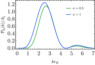
Figure 1: The integrand of the linear variance in Eq. (How well do we know the primordial black hole abundance? The crucial role of nonlinearities when approaching the horizon) for a lognormal curvature perturbation power spectrum ${\cal P}_{\zeta}(k)=A_{\zeta}\,{\rm exp}\left[-\ln(2k/3k_{\star})^{2}/2\sigma^{2}\right]$, assuming $k_{\star}r_{m}=2.1\,(1.75)$ for different widths $\sigma=0.5\,(1)$.

A critical look at the standard PBH abundance calculation. At this stage one can outline a few inconsistencies in the standard calculation of the PBH abundance:

i) The initial density perturbation is defined on superhorizon scales, and then evolved forward through horizon re-entry to check if a PBH will form. The starting point, Eq. (2), to calculate the threshold is rigorously valid only on superhorizon scales, much before the large overdensities re-enter the Hubble radius. The threshold is computed by using the time-independent part of the profile at times such that $r_{m}\gg r_{H}$, and then extrapolating its value at horizon crossing, for which $\epsilon(t_{H})=1$, with the growth in time $\sim(aH)^{-2}\sim a^{2}$. This procedure based on the gradient expansion breaks down close to horizon crossing and neglects the effect of the radiation pressure, which would be increasingly more important as we approach horizon crossing. This is clear from the expression (5) where there is no radiation transfer function.

The point is that the variance $\sigma_{l}^{2}$, which contains the information of the radiation pressure through the linear radiation transfer function, is obtained by integrating over all momenta and the integrand in its definition, Eq. (How well do we know the primordial black hole abundance? The crucial role of nonlinearities when approaching the horizon), is peaked at scales beneath the horizon. Fig. 1 shows this point for some representative examples of comoving curvature perturbation power spectra.

This means that the variance gets contributions from scales which at $\epsilon(t_{H})=1$ are already well inside the horizon. The action of the radiation pressure becomes so important that the density contrast stops growing, thus changing completely the time dependence with respect to the linearly extrapolated case with no radiation pressure. This is because, for the relevant scales, the time dependence in the square root of the variance is of the form (up to oscillations) $\sim(aH)^{-2}T(k/aH)\sim$ constant.

The comparison between the extrapolated threshold with no transfer function and $\sigma_{l}$, which determines the PBH abundance, is therefore not much consistent. Even at the linear level the time dependence between the threshold, which is computed considering only cosmic expansion and without pressure effects at horizon crossing, and the square root of the variance does not cancel in the standard procedure.

One could of course compute both the density contrast and the square root of the variance on superhorizon scales to cancel the time dependence. This would require computing the variance without including the radiation transfer function Young (2019); Yoo et al. (2018, 2021). However, the integral over the momenta in the variance would be sensitive to the ultraviolet cut-off due to the $\sim k^{4}$ term and therefore again sensitive to the details around horizon crossing.

Forgetting the issue introduced by the radiation pressure and accounted for by the radiation transfer function does not come without a price already at the linear level. Indeed, calling $k_{\star}$ the typical momentum at which PBHs form, one has typically at the linear level $k_{\star}r_{m}\simeq k_{\star}/aH\simeq{\cal O}(2\div 3)$ Germani and Musco (2019); Musco (2019), and $T^{2}(k_{\star}r_{m})\simeq(0.76\div 0.53)$. The effect of the transfer function is not negligible because the length scale $\sim k_{\star}^{-1}$ is already well inside the horizon when $r_{m}\simeq r_{H}$. The radiation pressure therefore tends to suppress the variance and makes it more difficult to build up perturbations able to overcome a given barrier. As we shall see, this remains true at second-order.

ii) The quantity $\delta_{m}$ is intrinsically of the second-order. Evaluating the effects of the radiation pressure will therefore require at least a second-order transfer function to be consistent both for the calculation of the threshold and the variance. This is a major source of uncertainty in the calculation of the PBH abundance. In the following we will adopt a perturbative approach to discuss the role of non-linearities in the evolution of the density contrast by expanding each quantity as $\mathcal{O}(t,{\bf x})=\mathcal{O}_{1}(t,{\bf x})+\mathcal{O}_{2}(t,{\bf x})/2+\cdots$ (see the Appendix for the perturbative expansion of the cosmological perturbations).

Consider the density contrast in the comoving gauge of Eq. (2) close to the Hubble crossing time $t_{H}$ and imagine an effective expansion at second-order of the form

$$\delta^{\text{\tiny com}}(t_{H},{\bf x}) =f_{\zeta}(t_{H})\nabla^{2}\zeta_{1}({\bf x})$$

$$+g_{\zeta}(t_{H})\zeta_{1}({\bf x})\nabla^{2}\zeta_{1}({\bf x})$$

$$+h_{\zeta}(t_{H})\partial_{i}\zeta_{1}({\bf x})\partial^{i}\zeta_{1}({\bf x})+\cdots,$$ (13)

in terms of some time-dependent functions $f_{\zeta}(t_{H})$, $g_{\zeta}(t_{H})$, $h_{\zeta}(t_{H})$, $\cdots$. The variance of such a quantity will depend only (assuming $\zeta_{1}({\bf x})$ is a Gaussian field) upon the square root of the combination

$$f_{\zeta}^{2}(t_{H})\langle(\nabla^{2}\zeta_{1})^{2}\rangle+g^{2}_{\zeta}(t_{H})\langle(\zeta_{1}\nabla^{2}\zeta_{1})^{2}\rangle+\cdots,$$ (14)

as $\zeta_{1}({\bf x})$ is treated as a stochastic quantity. The threshold, on the other hand, is determined from the profile in real space, and will depend on the linear combination of the functions $f_{\zeta}(t_{H})$, $g_{\zeta}(t_{H})$, $h_{\zeta}(t_{H})$, $\cdots$. Since close to the horizon the functions are not expected to have the same time dependence, the cancellation operating at the linear level will be in general no longer operative;

iii) The threshold $\delta_{c}$ (or $\delta_{l,c}$) is routinely calculated extrapolating its value at horizon crossing in an unperturbed universe. However, it has been already noted that the non-linear effects arising at the true horizon crossing in an inhomogeneous universe, where the gradient expansion fails, increase the value of the threshold by about a factor ${\cal O}(1.7\div 2)$ with respect to the one computed on superhorizon scales and linearly extrapolated at $\epsilon(t_{H})=1$ Musco et al. (2021) (see their Fig. 8). Part of this extra growth is due to the longer time necessary to reach the non-linear horizon crossing, part is due to higher orders in the gradient expansion when $\epsilon(t_{H})\sim 1$ and finally part to non-linear effects due to the radiation pressure, which are accounted for numerically in Ref. Musco et al. (2021). In general, increasing the critical threshold by a factor ${\cal O}(1.7\div 2)$ might drastically reduce the PBH abundance, unless the variance of the density contrast does increase correspondingly.

Overall, non-linear effects become important close to horizon crossing and may give rise to large corrections to the probability of collapse estimated in the literature.

The rest of the paper is dedicated to inspect more closely such sources of uncertainties due to non-linear effects. We start by commenting about the last point we mentioned.

Crossing the real horizon later. There are various effects to consider. First, the physical horizon in a perturbed universe expands more slowly than in an unperturbed universe, making the density profile grow more. Secondly, non-linear effects and the effect of the radiation pressure close to the horizon crossing change the density contrast profile; both lead to an increase of the critical threshold, as discussed numerically in Section 5 of Ref. Musco et al. (2021).

We discuss here the first effect, which is already present at horizon crossing at the linear level, and we will come back to the second effect in the next section.

Consider the equation describing the expansion rate $H(t,{\bf x})$ as measured by a free-falling observer which is instantaneously at rest with respect to the radiation fluid, i.e. on comoving slicings Liddle and Lyth (2000)

$$H^{2}(t,{\bf x})=H^{2}(t)\Big{(}1+\delta_{1}^{\text{\tiny com}}(t,{\bf x})\Big{)}+\frac{2}{3}\frac{\nabla^{2}}{a^{2}}\zeta_{1}(t,{\bf x}).$$ (15)

Since for large amplitudes the peaks of the density contrast are identifiable with the peaks of the comoving curvature perturbation De Luca et al. (2019) for which $\nabla^{2}\zeta_{1}<0$, we automatically deduce that the physical Hubble rate is smaller than the background value provided that the last term in Eq. (15) is larger than the term $H^{2}(t)\delta_{1}^{\text{\tiny com}}$. One can easily convince oneself that this is indeed the case.

At the linear level and for any scale (not only superhorizon), one can relate the linear density contrast in the comoving gauge to the linear gauge-invariant Bardeen’s potential $\Phi_{1}(t,{\bf x})$ through the following equation Malik and Wands (2009) (see also the Appendix):

$$\delta_{1}^{\text{\tiny com}}(t,{\bf x})=\frac{2}{3}\frac{\nabla^{2}\Phi_{1}(t,{\bf x})}{a^{2}H^{2}}.$$ (16)

Approximating at horizon crossing $\Phi_{1}(t_{H},{\bf x})\simeq-2\zeta_{1}({\bf x})/3$, one obtains

$$H^{2}(t_{H},{\bf x})\simeq H^{2}(t_{H})\left(1-\frac{1}{2}\delta_{1}^{\text{\tiny com}}(t_{H},{\bf x})\right).$$ (17)

One can estimate the effect on the threshold by averaging over a sphere of radius $r_{m}$ and assuming the critical profile for $\delta_{1}^{\text{\tiny com}}(t_{H},{\bf x})$, obtaining

$$\frac{3}{r_{m}^{3}}\int_{0}^{r_{m}}{\rm d}r\,r^{2}\left(\frac{H^{2}(t_{H},{\bf x})}{H^{2}(t_{H})}-1\right)\simeq-\frac{1}{2}\delta_{c},$$ (18)

from which one can see already the effect of the curvature term in slowing down the Hubble radius expansion. In the last equation, to be consistent with the linear perturbation theory adopted so far, one needs to take the value of $\delta_{c}$ obtained from the linear Gaussian threshold Musco et al. (2021) for the volume average of the first-order density contrast $\delta_{1}^{\text{\tiny com}}(t_{H},{\bf x})$.

One can do a better estimate including the effect of higher-order gradients, still remaining at the linear level. At horizon crossing, the comoving curvature term starts growing due to the scalar shear and the effect of higher-order gradients starts becoming manifest Malik and Wands (2009)

$$\frac{\dot{\zeta}_{1}}{H}\simeq\frac{1}{4}\delta^{\text{\tiny com}}_{1}-\frac{3}{4}\frac{\nabla^{2}\delta_{1}^{\text{\tiny com}}}{a^{2}H^{2}},$$ (19)

where the dot denotes differentiation with respect to the cosmic time. The rate $\dot{\zeta}_{1}$ is positive since the second term grows faster (as $a^{2}$) than the first one and around the peak of the density contrast $\nabla^{2}\delta_{1}^{\text{\tiny com}}<0$. Integrating over time and inserting the result in Eq. (15) gives

$$\left(\frac{H^{2}(t_{H},{\bf x})}{H^{2}(t_{H})}-1\right) \simeq\delta_{1}^{\text{\tiny com}}+\frac{1}{12}\frac{\nabla^{2}\delta_{1}^{\text{\tiny com}}}{a^{2}H^{2}}-\frac{1}{4}\frac{\nabla^{4}\delta_{1}^{\text{\tiny com}}}{a^{4}H^{4}}.$$ (20)

When the perturbation has just crossed the horizon, the last two terms dominate and averaging again over a sphere of radius $r_{m}$ we obtain an extra shift in the Hubble rate

$$\frac{3}{r_{m}^{3}}\int_{0}^{r_{m}}{\rm d}r\,r^{2}\left(\frac{H^{2}(t_{H},{\bf x})}{H^{2}(t_{H})}-1\right)$$

$$\simeq\frac{7}{4}r_{m}{\delta_{1}^{\prime}}^{\text{\tiny com}}(r_{m})-\frac{3}{2}r_{m}^{2}{\delta_{1}^{\prime\prime}}^{\text{\tiny com}}(r_{m})-\frac{3}{4}r_{m}^{3}{\delta_{1}^{\prime\prime\prime}}^{\text{\tiny com}}(r_{m})$$

$$\sim-\frac{5}{2}\delta_{1}^{\text{\tiny com}}(r_{m})\sim-\frac{5}{6}\delta_{c},$$ (21)

where we have approximated $r_{m}{\delta_{1}^{\prime}}^{\text{\tiny com}}(r_{m})\sim-r_{m}^{2}{\delta_{1}^{\prime\prime}}^{\text{\tiny com}}(r_{m})\sim r_{m}^{3}{\delta_{1}^{\prime\prime\prime}}^{\text{\tiny com}}(r_{m})\sim-{\delta_{1}^{\text{\tiny com}}}(r_{m})$ for a peaked perturbation, and used the relation $\delta_{c}=3\delta_{1}^{\text{\tiny com}}(t_{H},r_{m})$ for the critical profile Musco (2019), to get an order of magnitude estimate. Taking $\delta_{c}\simeq 0.51$ for the linear Gaussian threshold Musco et al. (2021), we obtain a change in the horizon-crossing time $\epsilon(t_{H})\propto 1/H$ of

$$\epsilon(t_{H})\simeq\frac{1}{\left(1-5\delta_{c}/6\right)^{1/2}}\simeq 1.3,$$ (22)

which is already in good agreement with what was numerically found in Ref. Musco et al. (2021) (see their Fig. 5, where a monochromatic spectrum corresponds formally to the case $\alpha=6.33$).

Being the variance dominated by the momentum modes well inside the horizon at $r_{m}=r_{H}$, when the linear density contrast has already stopped growing, increasing $\epsilon(t_{H})$ will not necessarily change the linear variance by the same factor. For instance, for a broad spectrum of the curvature perturbation, the linear variance does not change shifting $r_{H}$ as the integral is over the momenta $kr_{H}$ once $r_{m}$ is set to be equal to $r_{H}$. For a monochromatic power spectrum ${\cal P}_{\zeta}(k)=A_{\zeta}k_{\star}\delta(k-k_{\star})$, the change of the variance is set by the square of the radiation transfer function and it does not automatically cancel the change of $\epsilon^{2}(t_{H})$ in the critical threshold.

We do not attempt here to calculate the effect of non-linearities on the slowing down of horizon crossing, which have been studied numerically in Ref. Musco et al. (2021). We limit ourselves to the observation that one expects corrections of the order of ${\cal O}(\delta_{c}^{2})$, see for instance Eq. (A.21) of the Appendix. For instance, the leading (and growing in time) second-order correction to the comoving curvature perturbation at horizon crossing has the form Bartolo et al. (2004); Malik and Wands (2009); Inomata (2021)

$$\frac{2}{3}\nabla^{2}\zeta_{2}(t,{\bf x})\simeq-\frac{1}{48a^{2}H^{2}}\sum_{i\neq j}\partial_{i}\partial_{j}\delta_{1}^{\text{\tiny com}}(t,{\bf x})\partial^{i}\partial^{j}\delta_{1}^{\text{\tiny com}}(t,{\bf x}),$$ (23)

which is again negative and increasing like $a^{2}$. Its effect is to further slow down the expansion rate and increase the PBH threshold, but only for non-spherical peaks.

The non-linear transfer function: the second-order case. As we have stressed in the introduction, one of the main uncertainties in the calculation of the PBH abundance is that the effect of the radiation pressure is standardly either not accounted for (in the threshold, with the exception of Ref. Musco et al. (2021)) or it is, but only at the linear level (in the variance). We would like to offer some considerations about the non-linear effects, limiting ourselves to the second-order.

Our starting point is the second-order equation for the density contrast in the comoving orthogonal gauge expressed in terms of the Bardeen potentials constructed from the longitudinal gauge (see the Appendix)

$$\frac{3}{2}a^{2}H^{2}\delta_{2}^{\text{\tiny com}} =\nabla^{2}\Psi_{2}+3\partial_{i}\Phi_{1}\,\partial^{i}\Phi_{1}+8\Phi_{1}\nabla^{2}\Phi_{1}$$

$$+3\dot{\Phi}_{1}^{2}+\frac{6H}{\nabla^{2}}\left(\partial^{i}\dot{\Phi}_{1}\partial_{i}{\Phi_{1}}+\dot{\Phi}_{1}\nabla^{2}{\Phi_{1}}\right).$$ (24)

This expression is valid at all scales, not only on superhorizon. It shows a fundamental point, that close to horizon crossing the overdensity on comoving orthogonal slices contains many non-linear terms, even non-local, and therefore it is unlikely that the non-linear smoothed density contrast will have a quadratic relation of the local type with the linear one, as in Eq. (7). In other words, Eq. (7), obtained on superhorizon scales, fails to capture the non-linearities in the critical threshold due to the radiation pressure. This implies that neither $\delta_{c}$ nor $\delta_{l,c}$ may be used and that a priori there is no simple relation of the local type between the linear density contrast and the non-linear one.

Eq. (How well do we know the primordial black hole abundance? The crucial role of nonlinearities when approaching the horizon) needs to be supplemented with the equation for the evolution of the second-order gravitational potential $\Psi_{2}$ Bartolo et al. (2007); Inomata (2021)

$${\ddot{\Psi}_{2}}+5H{\dot{\Psi}_{2}}-\frac{1}{3}\frac{\nabla^{2}\Psi_{2}}{a^{2}} =\frac{1}{a^{2}}\left[\frac{2}{3}\partial^{i}\Phi_{1}\partial_{i}\Phi_{1}+\frac{8}{3}\Phi_{1}\nabla^{2}\Phi_{1}\right.$$

$$+2{\dot{\Phi}_{1}}^{2}+HN^{j}_{\,\,\,i}\left(A^{(2)i}_{\,\,j}\right)^{\cdot}$$

$$+\left.\frac{1}{3}N^{j}_{\,\,\,i}\left(A^{(2)i}_{\,\,j}\right)^{,k}_{,k}\right]$$ (25)

$$A^{(2)i}_{\,\,j} =6\,\partial^{i}\Phi_{1}\partial_{j}\Phi_{1}+\frac{2}{H}\left(\partial^{i}\Phi_{1}\partial_{j}\Phi_{1}\right)^{\cdot}$$

$$+\frac{2}{H^{2}}\partial^{i}\dot{\Phi}_{1}\partial_{j}\dot{\Phi}_{1},$$

where

$$N^{j}_{\,\,\,i}=\frac{3}{2}\frac{1}{\nabla^{2}}\left(\frac{\partial^{j}\partial_{i}}{\nabla^{2}}-\frac{1}{3}\delta^{j}_{\,\,\,i}\right).$$ (26)

Eq. (How well do we know the primordial black hole abundance? The crucial role of nonlinearities when approaching the horizon) has to be solved with the superhorizon initial condition Bartolo et al. (2006, 2007)

$${\Psi_{2}}({\bf x})=-2\Phi^{2}_{1}({\bf x})+2N^{j}_{\,\,\,i}\left(\partial^{i}\Phi_{1}({\bf x})\partial_{j}\Phi_{1}({\bf x})\right).$$ (27)

In momentum space the solution is the sum of two pieces

$${\Psi_{2}}(t,{\bf k})={\Psi_{2}}({\bf k})T(k/aH)$$

$$+\int\frac{{\rm d}^{3}p}{(2\pi)^{3}}uv\left(\frac{2}{3}\right)^{2}I_{\Psi}\left(u,v,\frac{k}{aH}\right)\zeta_{1}(\bf p)\zeta_{1}({\bf k}-{\bf p}),$$ (28)

where $u=|{\bf k}-{\bf p}|/k$, $v=p/k$. This equation shows the dependence on the linear radiation transfer function in the first term and of the second-order radiation transfer function through the function $I_{\Psi}(u,v,x)$ Bartolo et al. (2006, 2007); Inomata (2021).

To account for the effect of the radiation pressure in the PBH threshold at second-order in perturbation theory we proceed as follows. At first-order the equation of motion of the gravitational potential is

$${\ddot{\Phi}_{1}}+5H{\dot{\Phi}_{1}}-\frac{1}{3}\frac{\nabla^{2}\Phi_{1}}{a^{2}}=0.$$ (29)

We can treat the last term as a perturbation, which gives close to horizon crossing

$$\Phi_{1}(t,{\bf x}) =\int^{t}\frac{{\rm d}t^{\prime}}{a^{5}(t^{\prime})}\int^{t^{\prime}}{\rm d}t^{\prime\prime}a^{5}(t^{\prime\prime})\frac{1}{3}\frac{\nabla^{2}\Phi_{1}({\bf x})}{a^{2}(t^{\prime\prime})}$$

$$=\left(1+\frac{1}{30}\frac{\nabla^{2}}{a^{2}H^{2}}\right)\Phi_{1}({\bf x}).$$ (30)

This is quite a good approximation: going to momentum space and evaluating at $k_{\star}r_{m}\simeq k_{\star}r_{H}=2.74$ for a monochromatic power spectrum, we find $\Phi_{1}(t,{\bf x})\simeq 0.75\Phi_{1}({\bf x})$, while the linear radiation transfer function gives $T(2.74)\Phi_{1}({\bf x})=0.77\Phi_{1}({\bf x})$.

At second-order, proceeding in a similar way to obtain $\Psi_{2}(t,{\bf x})$ by using Eq. (27), then shown in Eq. (How well do we know the primordial black hole abundance? The crucial role of nonlinearities when approaching the horizon), we obtain (see the Appendix for details)

$$\delta_{2}^{\text{\tiny com}} \simeq\frac{1}{a^{2}H^{2}}\left(\frac{2}{3}\nabla^{2}\Psi_{2}+2\partial_{i}\Phi_{1}\,\partial^{i}\Phi_{1}+\frac{16}{3}\Phi_{1}\nabla^{2}\Phi_{1}\right)$$

$$=\frac{1}{a^{2}H^{2}}\left(-\frac{4}{3}\nabla^{2}\Phi^{2}_{1}({\bf x})+2\frac{\partial^{j}\partial_{i}}{\nabla^{2}}(\partial^{i}\Phi_{1}({\bf x})\partial_{j}\Phi_{1}({\bf x}))\right.$$

$$\left.+\frac{4}{3}\partial^{i}\Phi_{1}({\bf x})\partial_{i}\Phi_{1}({\bf x})+\frac{16}{3}\Phi_{1}\nabla^{2}\Phi_{1}\right)$$

$$+\frac{1}{a^{4}H^{4}}\left(\frac{2}{3}\partial^{i}\nabla^{2}\Phi_{1}({\bf x})\partial_{i}\Phi_{1}({\bf x})\right.$$

$$\left.+\frac{8}{15}\nabla^{2}\Phi_{1}({\bf x})\nabla^{2}\Phi_{1}({\bf x})+\frac{2}{15}\Phi_{1}({\bf x})\nabla^{4}\Phi_{1}({\bf x})\right).$$ (31)

When evaluated at the time of horizon crossing $aH=1/r_{H}\simeq 1/r_{m}$, the first-order curvature profile $\Phi_{1}(t_{H},{\bf x})\simeq-2\zeta_{1}({\bf x})/3$ in Fourier space is dominated by large momenta, see for instance Fig. 1 for different shapes of a lognormal power spectrum. This allows us to focus only on the last three lines in the previous expression, which are expected to dominate for large momenta.

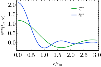
Figure 2: The density profile corresponding to the critical threshold at first- and second-order in perturbation theory, for a monochromatic curvature spectrum.

At horizon crossing the density contrast becomes

$$\delta_{2}^{\text{\tiny com}}(t_{H},{\bf x}) \simeq\frac{4r_{m}^{4}}{9}\left(\frac{2}{3}\partial^{i}\nabla^{2}\zeta_{1}({\bf x})\partial_{i}\zeta_{1}({\bf x})\right.$$

$$\left.+\frac{8}{15}\nabla^{2}\zeta_{1}({\bf x})\nabla^{2}\zeta_{1}({\bf x})+\frac{2}{15}\zeta_{1}({\bf x})\nabla^{4}\zeta_{1}({\bf x})\right).$$ (32)

Adopting Gaussian peak theory to a monochromatic curvature perturbation power spectrum, for which $k_{\star}r_{m}\simeq 2.74$, one can derive the shape for the linear curvature profile Musco et al. (2021)

$$\zeta_{1}({\bf x})=\zeta_{0}\frac{\sin(k_{\star}r)}{k_{\star}r},$$ (33)

from which we obtain the critical density profile at second-order shown in Fig. 2, where the overall amplitude $\zeta_{0}$ has been fixed at the linear level by requiring that $\delta_{c}=0.51=3\delta_{1}^{\text{\tiny com}}(t_{H},r_{m})$ Musco (2019). The impact of the second-order radiation transfer function on the PBH threshold is estimated to be

$$\frac{3}{r_{m}^{3}}\int_{0}^{r_{m}}{\rm d}rr^{2}\delta_{2}^{\text{\tiny com}}(t_{H},r)\simeq 0.13.$$ (34)

This result shows that the second-order radiation transfer function increases further the PBH threshold for a monochromatic spectrum, due to the radiation pressure which makes the collapse of the overdensities into a PBH more difficult. To this effect one should further add the one described in the previous section related to the slowing down of the horizon. The corresponding critical threshold will be given roughly by (the factor $1/2$ comes from the normalization of the second-order variables)

$$\epsilon^{2}(t_{H})\delta_{c}+\frac{1}{2}\epsilon^{4}(t_{H})\frac{3}{r_{m}^{3}}\int_{0}^{r_{m}}{\rm d}rr^{2}\delta_{2}^{\text{\tiny com}}\simeq 1.08,$$ (35)

where the corrective factor $\epsilon^{4}(t_{H})$ has been included for the slowing down of the horizon based on the dependence $1/(aH)^{4}$ in Eq. (How well do we know the primordial black hole abundance? The crucial role of nonlinearities when approaching the horizon). This result is in good agreement with the numerical fit for the PBH threshold, $\alpha^{0.06}+0.025\simeq 1.14$, for a monochromatic curvature power spectrum with $\alpha=6.33$, provided in Ref. Musco et al. (2021) (see also the left panel of their Fig. 8).

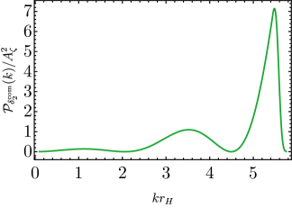
Figure 3: The integrand of the second-order variance in Eq. (How well do we know the primordial black hole abundance? The crucial role of nonlinearities when approaching the horizon) for a monochromatic curvature perturbation power spectrum evaluated at the time of horizon crossing.

As for the variance at second-order, we offer the following considerations. When a given scale re-enters the horizon, the linear gravitational potential $\Phi_{1}(t,{\bf x})$ decays like $a^{-2}$ (up to oscillations). By inspecting the time dependence of Eq. (How well do we know the primordial black hole abundance? The crucial role of nonlinearities when approaching the horizon) it is easy to convince ourselves that the second-order gravitational potential $\Psi_{2}(t,{\bf x})$ decays like $a^{-2}$ as well Inomata (2021). As a consequence, one can keep the leading time dependent term in Eq. (How well do we know the primordial black hole abundance? The crucial role of nonlinearities when approaching the horizon) and approximate

$$\frac{3}{2}a^{2}H^{2}\delta_{2}^{\text{\tiny com}}\simeq\nabla^{2}\Psi_{2},$$ (36)

because all the other terms decay faster at horizon crossing. From the solution of the second-order scalar perturbation in Eq. (How well do we know the primordial black hole abundance? The crucial role of nonlinearities when approaching the horizon), one can estimate the variance of the second-order smoothed density contrast in the comoving gauge at horizon crossing by computing its two-point connected correlation function, which gives

$$\sigma_{2}^{2} =\int\frac{{\rm d}k}{k}{\cal P}_{\delta_{2}^{\text{\tiny com}}}(k,r_{H}),$$

$${\cal P}_{\delta_{2}^{\text{\tiny com}}}(k,r_{H}) =\int_{0}^{\infty}{\rm d}v\int_{|v-1|}^{v+1}{\rm d}u\left(\frac{2}{3}\right)^{6}(kr_{H})^{4}I^{2}_{\Psi}(u,v,kr_{H})$$

$$\cdot W^{2}(k,r_{m}){\mathcal{P}}_{\zeta_{1}}(kv){\mathcal{P}}_{\zeta_{1}}(ku).$$ (37)

In Fig. 3 we plot the power spectrum of the second-order smoothed density contrast in the comoving gauge for a monochromatic curvature perturbation power spectrum, for which we get

$${\cal P}_{\delta_{2}^{\text{\tiny com}}}(k,r_{H}) =\left(\frac{2}{3}\right)^{6}(kr_{H})^{4}\left(\frac{k_{\star}}{k}\right)^{2}W^{2}(k_{\star},r_{m})$$

$$\cdot I^{2}_{\Psi}\left(\frac{k_{\star}}{k},\frac{k_{\star}}{k},k_{\star}r_{H}\right)\theta\left(2-\frac{k}{k_{\star}}\right),$$ (38)

evaluated for $k_{\star}r_{m}\simeq k_{\star}r_{H}=2.74$, where $\theta$ indicates the Heaviside step function. The figure confirms that, as in the linear case, the variance is dominated by momenta larger than the Hubble rate where the second-order radiation transfer function is non-negligible. At this stage the time dependence $\sim a^{-2}$ of the gravitational potential $\Psi_{2}$ is the same as at the linear level and the second-order variance does not change as well with time (up to oscillations). The values of the linear and second-order variances for $k_{\star}r_{m}=2.74$ are (the factor $1/4$ in the second-order term accounts for the normalization of the second-order density contrast)

$$\sigma_{l}^{2}\simeq 1.19\,(0.41)\,A_{\zeta}\,\,\,{\rm and}{\,\,\,}\frac{1}{4}\sigma_{2}^{2}\simeq 0.25\,(1.02)\,A_{\zeta}^{2},$$ (39)

where in the parenthesis we have indicated the values when the Hubble rate is shifted by a factor $\epsilon(t_{H})\simeq 1.3$ due to the crossing of the physical horizon, as discussed in the previous section. We deduce that the second-order contribution is always negligible compared to the linear one, even for the preferred value of $A_{\zeta}\simeq 6\cdot 10^{-2}$ to explain the recent PTA data Franciolini et al. (2023). We think this conclusion is quite robust and does not depend on the details of the time of horizon crossing and the shape of the comoving curvature power spectrum, as long as $k_{\star}r_{m}\mathrel{\hbox to0.0pt{\lower 4.0pt\hbox{\hskip 0.5pt$\sim$}\hss}\raise 1.0pt\hbox{$>$}}1$. For instance, for a broad spectrum, even at second-order the variance is insensitive to changes in the physical horizon as it is an integral over all the momenta $kr_{H}$ once one sets $r_{m}=r_{H}$ at the corresponding order in perturbation theory.

As a final remark we notice that, because of the non-Gaussian nature of the second-order density contrast $\delta_{2}^{\text{\tiny com}}$, the expression for the PBH probability will depend also on higher-order cumulants of the density field beyond the two-point function. We leave the investigation of the form of such a probability to future work.

Conclusions. In this article we have addressed various issues related to the calculation of the abundance of PBHs and point out the uncertainties the standard procedure suffers of. They come above all from the incomplete treatment of the radiation pressure and of the non-linear effects close to horizon crossing.

Even if our calculations are certainly incomplete, we can offer the following hints: i) the critical threshold is larger than what routinely assumed. We have provided some physical explanations for such an increase; ii) The variance of the non-linear density contrast is unlikely to be changed with respect to the linear one. This is because it is suppressed by an extra power of the curvature perturbation power spectrum; iii) The time dependence between the critical threshold and the square root of the variance does not cancel at horizon crossing as the latter is dominated by momenta larger than the horizon, when the density contrast has already frozen in (up to oscillations). This is because the characteristic length scale is such that $k_{\star}^{-1}\mathrel{\hbox to0.0pt{\lower 4.0pt\hbox{\hskip 0.5pt$\sim$}\hss}\raise 1.0pt\hbox{$>$}}r_{m}\simeq r_{H}$. The reason why the linear and non-linear variances are suppressed is because of the action of the radiation pressure at the scales close to $k_{\star}$. Therefore, it is difficult to build up fluctuations which overcome a given barrier; iv) The relation between the non-linear and linear threshold is not of the local type, therefore making the calculation of the formation probability not straightforward; v) Given the fact that the non-linear effects increase the critical threshold, but not the variance, it is likely that the PBH abundance is much smaller than what considered in the literature so far.

If confirmed by a more complete all-order (most likely numerical) calculation, such conclusions would make the PTA data compatible with the PBH scenario, since the same amplitude of the stochastic GW background would correspond to much smaller PBH abundances.

Acknowledgments. We thank I. Musco for several discussions about the procedure to calculate the critical threshold and I. Musco and G. Franciolini for comments on the draft. V.DL. is supported by funds provided by the Center for Particle Cosmology at the University of Pennsylvania. A.R. is supported by the Boninchi Foundation for the project “PBHs in the Era of GW Astronomy”.

APPENDIX

The components of a perturbed spatially flat Robertson-Walker metric can be written, up to second-order and using conformal time, as (primes indicate here differentiation with respect to the conformal time $\tau$) Bartolo et al. (2007)

$$g_{00} =-a^{2}(\tau)\left(1+2\phi_{1}+\phi_{2}\right),$$

$$g_{0i} =a^{2}(\tau)\left(\hat{\omega}_{1i}+\frac{1}{2}\hat{\omega}_{2i}\right),$$

$$g_{ij} =a^{2}(\tau)\left[(1-2\psi_{1}-\psi_{2})\delta_{ij}+\left(\hat{\chi}_{1ij}+\frac{1}{2}\hat{\chi}_{2ij}\right)\right].$$ (A.1)

The standard splitting of the perturbations into scalar, transverse (i.e divergence-free) vector, and transverse trace-free tensor parts, with respect to the three-dimensional space with metric $\delta_{ij}$, can be performed in the following way:

$$\hat{\omega}_{i} =\partial_{i}\omega+\omega_{i},$$

$$\hat{\chi}_{ij} =D_{ij}\chi+\partial_{i}\chi_{j}+\partial_{j}\chi_{i}+\chi_{ij},$$ (A.2)

where $\omega_{i}$ and $\chi_{i}$ are transverse vectors ($\partial^{i}\omega_{i}=\partial^{i}\chi_{i}=0$), $\chi_{ij}$ is a symmetric transverse and trace-free tensor ($\partial^{i}\chi_{ij}=0$, $\chi_{i}^{~{}i}=0$) and $D_{ij}=\partial_{i}\partial_{j}-(1/3)\,\,\delta_{ij}\,\partial^{k}\partial_{k}$ is a trace-free operator. Here and in the following latin indices are raised and lowered using $\delta^{ij}$ and $\delta_{ij}$, respectively. For our purposes the metric in Eq. (How well do we know the primordial black hole abundance? The crucial role of nonlinearities when approaching the horizon) can be simplified. In fact, first-order vector perturbations are not generated during inflation and tensor modes are negligible. Thus, in the following we can neglect $\omega_{1i}$, $\chi_{1i}$ and $\chi_{1ij}$. However the same is not true for the second-order perturbations. In the second-order theory the second-order vector and tensor contributions can be generated by the first-order scalar perturbations even if they are initially zero. Thus we have to take them into account and we shall use the metric

$$g_{00} =-a^{2}(\tau)\left(1+2\phi_{1}+\phi_{2}\right),$$

$$g_{0i} =a^{2}(\tau)\left(\partial_{i}\omega_{1}+\frac{1}{2}\,\partial_{i}\omega_{2}+\frac{1}{2}\,\omega_{2i}\right),$$

$$g_{ij} =a^{2}(\tau)\left[\left(1-2\psi_{1}-\psi_{2}\right)\delta_{ij}+D_{ij}\left(\chi_{1}+\frac{1}{2}\chi_{2}\right)+\frac{1}{2}\left(\partial_{i}\chi_{2j}+\partial_{j}\chi_{2i}+\chi_{2ij}\right)\right].$$ (A.3)

The first-order perturbations of the Einstein tensor components which we need are

$${\delta}_{1}{G_{~{}0}^{0}} =\frac{1}{a^{2}}\Bigg{[}6\,\Big{(}\frac{a^{\prime}}{a}\Big{)}^{2}\phi_{1}\,+\,6\,\frac{a^{\prime}}{a}{\psi^{\prime}_{1}}\,+\,2\,\frac{a^{\prime}}{a}\partial_{i}\,\partial^{i}\omega_{1}-2\,\partial_{i}\,\partial^{i}\psi_{1}\,-\,\frac{1}{2}\,\partial_{k}\partial^{i}\,D^{k}_{i}\chi_{1}\Bigg{]},$$ (A.4)

$${\delta}_{1}{G^{0}_{~{}i}} =\frac{1}{a^{2}}\left(-\,2\,\frac{a^{\prime}}{a}\partial_{i}\phi_{1}\,-\,2\,\partial_{i}{\psi^{\prime}_{1}}\,-\,\frac{1}{2}\,\partial_{k}D^{k}_{~{}i}{\chi^{\prime}_{1}}\right).$$ (A.5)

At second-order they are

$${\delta}_{2}{G_{~{}0}^{0}} =\frac{1}{a^{2}}\Big{[}3\Big{(}\frac{a^{\prime}}{a}\Big{)}^{2}\phi_{2}\,+\,3\,\frac{a^{\prime}}{a}{\psi^{\prime}_{2}}\,-\,\partial_{i}\,\partial^{i}\psi_{2}+\frac{a^{\prime}}{a}\partial_{i}\,\partial^{i}\omega_{2}\,-\,\frac{1}{4}\partial_{k}\partial_{i}\,D^{ki}\chi_{2}-\,12\left(\frac{a^{\prime}}{a}\right)^{2}\left(\phi_{1}\right)^{2}$$

$$-12\,\frac{a^{\prime}}{a}\,\phi_{1}\,{\psi^{\prime}_{1}}-\,3\,\partial_{i}\psi_{1}\,\partial^{i}\psi_{1}\,-\,8\,\psi_{1}\ \partial_{i}\,\partial^{i}\psi_{1}-3\left({\psi^{\prime}_{1}}\right)^{2}\,+\,4\,\frac{a^{\prime}}{a}\,\phi_{1}\,\partial_{i}\,\partial^{i}\omega_{1}\,-\,2\,\frac{a^{\prime}}{a}\partial_{k}\omega_{1}\,\partial^{k}\phi_{1}$$

$$-\frac{1}{2}\frac{a^{\prime\prime}}{a}\,\partial_{k}\omega_{1}\,\partial^{k}\omega_{1}+\,12\,\frac{a^{\prime}}{a}\psi_{1}\,{\psi^{\prime}_{1}}+\frac{1}{2}\,\partial_{i}\partial_{k}\omega_{1}\,\partial^{i}\partial^{k}\omega_{1}-\,2\,\frac{a^{\prime}}{a}\partial_{k}\psi_{1}\,\partial^{k}\omega_{1}$$

$$+\,4\,\frac{a^{\prime}}{a}\psi_{1}\,\partial_{i}\,\partial^{i}\omega_{1}\,-\,\frac{1}{2}\,\partial_{k}\partial^{k}\omega_{1}\,\partial_{k}\partial^{k}\omega_{1}-2\,\partial_{k}\omega_{1}\,\partial^{k}{\psi^{\prime}_{1}}\,-\,2{\psi^{\prime}_{1}}\partial_{i}\,\partial^{i}\omega_{1}\,-\,\phi_{1}\,\partial_{i}\partial^{k}\,D^{i}_{~{}k}\chi_{1}$$

$$-\,2\,\psi_{1}\partial_{k}\partial^{i}\,D^{k}_{~{}i}\chi_{1}+\partial_{k}\partial_{i}\psi_{1}\,D^{ki}\chi_{1}-2\frac{a^{\prime}}{a}\partial_{i}\partial_{k}\omega_{1}\,D^{ik}\chi_{1}\,-\,2\,\frac{a^{\prime}}{a}\partial_{k}\omega_{1}\,\partial_{i}\,D^{ik}\chi_{1}$$

$$-\,\partial_{k}\omega_{1}\,\partial^{i}D^{k}_{~{}i}{\chi^{\prime}_{1}}-\frac{1}{2}\,\partial_{i}\,\partial^{i}\,D_{mk}\chi_{1}\,D^{km}\chi_{1}+\partial_{m}\partial^{k}\,D_{ik}\chi_{1}\,D^{im}\chi_{1}\,+\,\frac{1}{2}\,\partial_{k}D^{km}\chi_{1}\,\partial^{i}D_{mi}\chi_{1}$$

$$-\frac{1}{8}\,\partial^{i}D^{km}\chi_{1}\,\partial_{i}D_{km}\chi_{1}\,+\,\frac{1}{8}\,D^{ik}{\chi^{\prime}_{1}}\,D_{ki}{\chi^{\prime}_{1}}+\frac{a^{\prime}}{a}D^{ki}\chi_{1}\,D_{ik}{\chi^{\prime}_{1}}\Big{]},$$ (A.6)

$${\delta}_{2}{G^{0}_{~{}i}} =\frac{1}{a^{2}}\Big{(}-\frac{a^{\prime}}{a}\partial_{i}\phi_{2}\,-\,\partial_{i}{\psi^{\prime}_{2}}\,-\,\frac{1}{4}\partial_{k}\,D^{k}_{~{}i}{\chi^{\prime}_{2}}+\frac{1}{4}\partial_{k}\partial^{k}\omega_{2i}\,+8\frac{a^{\prime}}{a}\phi_{1}\partial_{i}\phi_{1}+\,4\,\phi_{1}\,\partial_{i}{\psi^{\prime}_{1}}+2\,{\psi^{\prime}_{1}}\partial_{i}\phi_{1}$$

$$-\,4\,{\psi^{\prime}_{1}}\partial_{i}\psi_{1}\,-\,4\,\psi_{1}\,\partial_{i}{\psi^{\prime}_{1}}\,+\,\partial_{i}\phi_{1}\,\partial_{i}\,\partial^{i}\omega_{1}-\partial_{i}\partial_{k}\omega_{1}\,\partial^{k}\phi_{1}+8\frac{a^{\prime\prime}}{a}\phi_{1}\,\partial_{i}\omega_{1}\,-\,4\Big{(}\frac{a^{\prime}}{a}\Big{)}^{2}\phi_{1}\,\partial_{i}\omega_{1}$$

$$-\,2\,\frac{a^{\prime}}{a}\,\partial^{k}\omega_{1}\,\partial_{i}\partial_{k}\omega_{1}\,+\,\partial_{i}\,\partial^{i}\psi_{1}\,\partial_{i}\omega_{1}+\partial^{k}\omega_{1}\,\,\partial_{i}\partial_{k}\psi_{1}\,-\,\partial_{k}\phi_{1}\,D^{k}_{~{}i}{\chi^{\prime}_{1}}\,+\,\frac{1}{2}\,\partial^{k}\phi_{1}\,D_{ik}{\chi^{\prime}_{1}}$$

$$-\psi_{1}\,\partial_{k}D^{k}_{~{}i}{\chi^{\prime}_{1}}+\,\frac{1}{2}\,\partial_{k}\psi_{1}\,D^{k}_{~{}i}{\chi^{\prime}_{1}}\,-\,{\psi^{\prime}_{1}}\partial_{k}D^{k}_{~{}i}\chi_{1}-\partial_{k}{\psi^{\prime}_{1}}D^{k}_{~{}i}\chi_{1}\,+\,\partial_{i}\omega_{1}\,\partial_{k}\partial^{m}\,D^{k}_{~{}m}\chi_{1}$$

$$+\,\Big{(}\frac{a^{\prime}}{a}\Big{)}^{2}\partial^{k}\omega_{1}\,D_{ik}\chi_{1}\,+\,\partial^{k}\omega_{1}\,\partial_{m}\partial_{i}\,D^{m}_{~{}k}\chi_{1}-\frac{1}{2}\,\partial^{m}\omega_{1}\,\partial_{k}\partial^{k}\,D_{im}\chi_{1}\,+\,\frac{1}{2}\,\partial_{k}D^{km}\chi_{1}\,D_{im}{\chi^{\prime}_{1}}$$

$$+\,\frac{1}{2}\,\partial_{k}D_{im}{\chi^{\prime}_{1}}\,D^{km}\chi_{1}-\frac{1}{4}\partial_{i}D_{mk}\chi_{1}\,D^{km}{\chi^{\prime}_{1}}-\frac{1}{2}\,\partial_{i}D_{mk}{\chi^{\prime}_{1}}\,D^{km}\chi_{1}-2\,\frac{a^{\prime\prime}}{a}\,\partial^{k}\omega_{1}\,D_{ik}\chi_{1}\Big{)}.$$ (A.7)

Correspondingly, the first-order components of the energy-momentum tensor are

$${\delta}_{1}{T_{~{}0}^{0}} =-\delta\rho_{1}\,$$

$${\delta}_{1}{T_{~{}i}^{0}} =(\rho_{0}+P_{0})(v_{1i}+\hat{\omega}_{1i}),$$ (A.8)

in terms of the background energy density $\rho_{0}$ and pressure $P_{0}$. At second-order they read

$${\delta}_{2}{T_{~{}0}^{0}} =-\frac{1}{2}\delta\rho_{2}-(\rho_{0}+P_{0})v_{1k}(v_{1}^{k}+\hat{\omega}_{1}^{k}),$$ (A.9)

$${\delta}_{2}{T_{~{}i}^{0}} =\frac{1}{2}(\rho_{0}+P_{0})\left[(v_{2i}+\hat{\omega}_{2i}-2\phi_{1}(v_{1i}+2\hat{\omega}_{1i})+4{\delta}_{1}g_{ik}v_{1}^{k}\right]+\frac{1}{2}(\delta\rho_{1}+\delta P_{1})(v_{1i}+\hat{\omega}_{1i}).$$ (A.10)

Einstein’s equations, as written in a generic gauge, are automatically gauge invariant and one can check that they can be written in terms of gauge-invariant quantities. One is therefore free to evaluate them in the most convenient gauge on the left- and on the right-hand side. For instance, we evaluate the first-order Einstein tensor in the generalized longitudinal gauge (also called Poisson gauge) for which $\hat{\omega}=\chi=0$, while we evaluate the energy-momentum tensor in the comoving orthogonal gauge for which $v_{i}=\hat{\omega}_{i}=0$. In such a case, one easily finds by subtracting Eqs. (A.4) and (A.5),

$$\nabla^{2}\Phi_{1}=\frac{3}{2}{\cal H}^{2}\delta_{1}^{\text{\tiny com}},$$ (A.11)

where $\Psi_{1}=\Phi_{1}$ are the Bardeen’s gauge-invariant potentials Bardeen (1980), ${\cal H}=a^{\prime}/a=aH$, and $\delta_{1}^{\text{\tiny com}}$ is the gauge-invariant density contrast in the comoving orthogonal gauge. Using the fact that in momentum space

$$\Phi_{1}(k,\tau)=-\frac{2}{3}T(k\tau)\zeta_{1}(k),$$ (A.12)

we get

$$\delta_{1}^{\text{\tiny com}}(k,\tau)=\frac{4}{9}\frac{k^{2}}{{\cal H}^{2}}T(k\tau)\zeta_{1}(k).$$ (A.13)

This equation is valid at all scales, not only on superhorizon scales. Similarly, at second-order one obtains the equations

$$-\frac{3}{2}{\cal H}^{2}\delta_{2}^{\text{\tiny com}} =3{\cal H}^{2}\Phi_{2}\,+\,3\,{\cal H}{\Psi^{\prime}_{2}}\,-\,\partial_{i}\,\partial^{i}\Psi_{2}-12{\cal H}^{2}\left(\Phi_{1}\right)^{2}-3\,\partial_{i}\Phi_{1}\,\partial^{i}\Phi_{1}\,-\,8\,\Phi_{1}\ \partial_{i}\,\partial^{i}\Phi_{1}-3\,\left({\Phi^{\prime}_{1}}\right)^{2},$$

$$0 =-\,{\cal H}\partial_{i}\Phi_{2}\,-\,\partial_{i}{\Psi^{\prime}_{2}}\,+8{\cal H}\Phi_{1}\partial_{i}\Phi_{1}-2\,{\Phi^{\prime}_{1}}\partial_{i}\Phi_{1},$$ (A.14)

which give

$$\frac{3}{2}{\cal H}^{2}\delta_{2}^{\text{\tiny com}} =\nabla^{2}\Psi_{2}+3\partial_{i}\Phi_{1}\,\partial^{i}\Phi_{1}+8\Phi_{1}\nabla^{2}\Phi_{1}+3\left({\Phi^{\prime}_{1}}\right)^{2}+\frac{6{\cal H}}{\nabla^{2}}\left(\partial^{i}{\Phi^{\prime}_{1}}\partial_{i}{\Phi_{1}}+{\Phi_{1}}^{\prime}\nabla^{2}{\Phi_{1}}\right),$$ (A.15)

which reproduces Eq. (How well do we know the primordial black hole abundance? The crucial role of nonlinearities when approaching the horizon) of the main text. The equation of motion for the second-order gravitational potential can be found in Refs. Bartolo et al. (2007); Inomata (2021) and during the radiation phase it reads

$${\Psi^{\prime\prime}_{2}}+4{\cal H}{\Psi^{\prime}_{2}}-\frac{1}{3}\nabla^{2}{\Psi_{2}} =\frac{2}{3}\partial^{i}\Phi_{1}\partial_{i}\Phi_{1}+\frac{8}{3}\Phi_{1}\nabla^{2}\Phi_{1}+2\left({\Phi^{\prime}_{1}}\right)^{2}+{\cal H}N^{j}_{\,\,\,i}\left(A^{i}_{2\,\,j}\right)^{\prime}+\frac{1}{3}N^{j}_{\,\,\,i}\left(A^{i}_{2\,\,j}\right)^{,k}_{,k},$$ (A.16)

$$A^{i}_{2\,\,j} =6\,\partial^{i}\Phi_{1}\partial_{j}\Phi_{1}+\frac{2}{{\cal H}}\left(\partial^{i}\Phi_{1}\partial_{j}\Phi_{1}\right)^{\prime}+\frac{2}{{\cal H}^{2}}\partial^{i}\Phi^{\prime}_{1}\partial_{j}\Phi^{\prime}_{1},$$ (A.17)

and

$$N^{j}_{\,\,\,i}=\frac{3}{2}\frac{1}{\nabla^{2}}\left(\frac{\partial^{j}\partial_{i}}{\nabla^{2}}-\frac{1}{3}\delta^{j}_{\,\,\,i}\right).$$ (A.18)

Eq. (A.16) has to be solved with the superhorizon initial condition (with $\Phi_{1}({\bf x})\simeq-2\zeta_{1}({\bf x})/3$) Inomata (2021)

$${\Psi_{2}}({\bf x})=-2\Phi_{1}^{2}({\bf x})+2N^{j}_{\,\,\,i}\left(\partial^{i}\Phi_{1}({\bf x})\partial_{j}\Phi_{1}({\bf x})\right)=-\frac{8}{9}\zeta_{1}^{2}({\bf x})+\frac{8}{9}N^{j}_{\,\,\,i}\left(\partial^{i}\zeta_{1}({\bf x})\partial_{j}\zeta_{1}({\bf x})\right),$$ (A.19)

and in momentum space the solution is the sum of two pieces

$${\Psi_{2}}(\tau,{\bf k})={\Psi_{2}}({\bf k})T(k\tau)+\int\frac{{\rm d}^{3}p}{(2\pi)^{3}}uvI_{\Psi}(u,v,k\tau)\left(\frac{2}{3}\right)^{2}\zeta_{1}(\bf p)\zeta_{1}({\bf k}-{\bf p}),$$ (A.20)

where $u=|{\bf k}-{\bf p}|/k$, $v=p/k$, and the function $I_{\Psi}$ can be found in Refs. Bartolo et al. (2006, 2007); Inomata (2021). A detailed inspection of the time behaviour of $I_{\Psi}(u,v,k\tau)$ shows that ${\Psi_{2}}(\tau,{\bf k})\propto a^{-2}$ due to the last term of Eq. (A.16) Inomata (2021).

Similarly, one can introduce the second-order curvature perturbation $\zeta_{2}$, which in the Newtonian gauge takes the form Bartolo et al. (2004); Malik and Wands (2009); Inomata (2021)

$$\zeta_{2}=-\Psi_{2}+\frac{1}{4}\delta_{2}+\frac{1}{16\mathcal{H}}\left(\delta_{1}^{2}\right)^{\prime}-\frac{1}{9}\delta_{1}^{2}-\frac{1}{1\mathcal{H}}\delta_{1}\left({\Phi^{\prime}_{1}}+2\mathcal{H}\Phi_{1}\right)-\frac{1}{32\mathcal{H}^{2}}\left[\delta_{1}^{,k}\delta_{1\,,k}-\nabla^{-2}\left(\delta_{1\,,i}\delta_{1\,,j}\right)^{,ij}\right].$$ (A.21)

On sub-horizon scales, where all gauges coincide and thus $\delta_{1}=\delta_{1}^{\text{\tiny com}}$, this expression provides the behaviour for the curvature perturbation at second-order. The last term represents the leading contribution at late time and one can show that

$$\frac{2}{3}\nabla^{2}\zeta_{2}(t,{\bf x})\simeq-\frac{1}{48a^{2}H^{2}}\sum_{i\neq j}\partial_{i}\partial_{j}\delta_{1}^{\text{\tiny com}}(t,{\bf x})\partial^{i}\partial^{j}\delta_{1}^{\text{\tiny com}}(t,{\bf x}),$$ (A.22)

as shown in Eq. (23) of the main text.

Finally, we provide the steps to estimate the second-order density contrast in the comoving gauge $\delta_{2}^{\text{\tiny com}}$, as shown in Eq. (How well do we know the primordial black hole abundance? The crucial role of nonlinearities when approaching the horizon) of the manuscript, which is needed to compute the corresponding impact on the threshold of PBH formation. Starting from Eq. (A.16) and treating the laplacian term $\nabla^{2}\Psi_{2}$ as a perturbation, we can rewrite the equation by introducing a source term $\mathcal{S}(t,{\bf x})$ as ${\ddot{\Psi}_{2}}+5H{\dot{\Psi}_{2}}=\mathcal{S}$ (working with cosmic time), such that its solution formally reads

$$\Psi_{2}(t,{\bf x}) =\int^{t}\frac{{\rm d}t^{\prime}}{a^{5}(t^{\prime})}\int^{t^{\prime}}{\rm d}t^{\prime\prime}a^{5}(t^{\prime\prime})\frac{\mathcal{S}({\bf x})}{a^{2}(t^{\prime\prime})},$$ (A.23)

where the source has been evaluated with proper superhorizon initial conditions, since we are interested in evaluating the density profile at the horizon crossing time. The equation then simplifies to

$$\Psi_{2}(t,{\bf x}) =\Psi_{2}({\bf x})+\int{\rm d}t\left(\frac{1}{15}\frac{\nabla^{2}\Psi_{2}}{a^{2}H}+\frac{1}{a^{2}H}\left[\frac{2}{15}\partial^{i}\Phi_{1}\partial_{i}\Phi_{1}+\frac{8}{15}\Phi_{1}\nabla^{2}\Phi_{1}+\frac{2}{5}N^{j}_{\,\,\,i}\nabla^{2}\left(\partial^{i}\Phi_{1}\partial_{j}\Phi_{1}\right)\right]\right)$$

$$=\Psi_{2}({\bf x})+\frac{1}{30}\frac{\nabla^{2}\Psi_{2}({\bf x})}{a^{2}H^{2}}+\frac{1}{a^{2}H^{2}}\left[\frac{1}{15}\partial^{i}\Phi_{1}\partial_{i}\Phi_{1}+\frac{4}{15}\Phi_{1}({\bf x})\nabla^{2}\Phi_{1}({\bf x})+\frac{1}{5}N^{j}_{\,\,\,i}\nabla^{2}\left(\partial^{i}\Phi_{1}({\bf x})\partial_{j}\Phi_{1}({\bf x})\right)\right].$$ (A.24)

By implementing the initial conditions shown in Eq. (A.19), we get after some simplifications

$$\Psi_{2}(t,{\bf x}) =-2\Phi^{2}_{1}({\bf x})+3\frac{1}{\nabla^{2}}\left(\frac{\partial^{j}\partial_{i}}{\nabla^{2}}-\frac{1}{3}\delta^{j}_{\,\,\,i}\right)\left(\partial^{i}\Phi_{1}({\bf x})\partial_{j}\Phi_{1}({\bf x})\right)-\frac{1}{5}\frac{1}{a^{2}H^{2}}\partial^{i}\Phi_{1}\partial_{i}\Phi_{1}+\frac{1}{10}\frac{1}{a^{2}H^{2}}\left(\frac{\partial^{j}\partial_{i}}{\nabla^{2}}\right)\left(\partial^{i}\Phi_{1}({\bf x})\partial_{j}\Phi_{1}({\bf x})\right)$$

$$+\frac{2}{15}\frac{1}{a^{2}H^{2}}\Phi_{1}\nabla^{2}\Phi_{1}+\frac{3}{10}\frac{1}{\nabla^{2}}\frac{1}{a^{2}H^{2}}\left(2\partial^{j}\nabla^{2}\Phi_{1}\partial_{j}\Phi_{1}+\nabla^{2}\Phi_{1}\nabla^{2}\Phi_{1}+\partial^{i}\partial^{j}\Phi_{1}\partial_{i}\partial_{j}\Phi_{1}\right),$$ (A.25)

where we have used that $\nabla^{2}\Phi_{1}^{2}=\partial^{i}\partial_{i}\Phi_{1}^{2}=\partial^{i}(2\Phi_{1}\partial_{i}\Phi_{1})=2\partial^{i}\Phi_{1}\partial_{i}\Phi_{1}+2\Phi_{1}\nabla^{2}\Phi_{1}$. By taking a Laplacian, we get

$$\nabla^{2}\Psi_{2}(t,{\bf x}) =-2\nabla^{2}\Phi^{2}_{1}({\bf x})+3\frac{\partial^{j}\partial_{i}}{\nabla^{2}}(\partial^{i}\Phi_{1}({\bf x})\partial_{j}\Phi_{1}({\bf x}))-\partial^{i}\Phi_{1}({\bf x})\partial_{i}\Phi_{1}({\bf x})$$

$$-\frac{2}{5}\frac{1}{a^{2}H^{2}}(\partial^{i}\nabla^{2}\Phi_{1}({\bf x})\partial_{i}\Phi_{1}({\bf x})+\partial^{i}\partial_{j}\Phi_{1}({\bf x})\partial_{i}\partial^{j}\Phi_{1}({\bf x}))$$

$$+\frac{1}{10}\frac{1}{a^{2}H^{2}}\left(2\partial^{j}\nabla^{2}\Phi_{1}({\bf x})\partial_{j}\Phi_{1}({\bf x})+\nabla^{2}\Phi_{1}({\bf x})\nabla^{2}\Phi_{1}({\bf x})+\partial^{i}\partial^{j}\Phi_{1}({\bf x})\partial_{i}\partial_{j}\Phi_{1}({\bf x})\right)$$

$$+\frac{2}{15}\frac{1}{a^{2}H^{2}}\left(\nabla^{2}\Phi_{1}({\bf x})\nabla^{2}\Phi_{1}({\bf x})+2\partial_{j}\Phi_{1}({\bf x})\partial^{j}\nabla^{2}\Phi_{1}({\bf x})+\Phi_{1}({\bf x})\nabla^{4}\Phi_{1}({\bf x})\right)$$

$$+\frac{3}{10}\frac{1}{a^{2}H^{2}}\left(2\partial^{j}\nabla^{2}\Phi_{1}({\bf x})\partial_{j}\Phi_{1}({\bf x})+\nabla^{2}\Phi_{1}({\bf x})\nabla^{2}\Phi_{1}({\bf x})+\partial^{i}\partial^{j}\Phi_{1}({\bf x})\partial_{i}\partial_{j}\Phi_{1}({\bf x})\right),$$ (A.26)

such that

$$\nabla^{2}\Psi_{2}(t,{\bf x})=-2\nabla^{2}\Phi^{2}_{1}({\bf x})+3\frac{\partial^{j}\partial_{i}}{\nabla^{2}}(\partial^{i}\Phi_{1}({\bf x})\partial_{j}\Phi_{1}({\bf x}))-\partial^{i}\Phi_{1}({\bf x})\partial_{i}\Phi_{1}({\bf x})$$

$$+\frac{1}{a^{2}H^{2}}\left(\frac{2}{3}\partial^{i}\nabla^{2}\Phi_{1}({\bf x})\partial_{i}\Phi_{1}({\bf x})+\frac{8}{15}\nabla^{2}\Phi_{1}({\bf x})\nabla^{2}\Phi_{1}({\bf x})+\frac{2}{15}\Phi_{1}({\bf x})\nabla^{4}\Phi_{1}({\bf x})\right).$$ (A.27)

The second-order density contrast then becomes

$$\delta_{2}^{\text{\tiny com}} =\frac{2}{3}\frac{1}{a^{2}H^{2}}\nabla^{2}\Psi^{(2)}+2\frac{1}{a^{2}H^{2}}\partial_{i}\Phi^{(1)}\,\partial^{i}\Phi^{(1)}+\frac{16}{3}\frac{1}{a^{2}H^{2}}\Phi^{(1)}\ \nabla^{2}\Phi^{(1)}$$

$$=\frac{1}{a^{2}H^{2}}\left(-\frac{4}{3}\nabla^{2}\Phi^{2}_{1}({\bf x})+2\frac{\partial^{j}\partial_{i}}{\nabla^{2}}(\partial^{i}\Phi_{1}({\bf x})\partial_{j}\Phi_{1}({\bf x}))+\frac{4}{3}\partial^{i}\Phi_{1}({\bf x})\partial_{i}\Phi_{1}({\bf x})+\frac{16}{3}\Phi^{(1)}\ \nabla^{2}\Phi^{(1)}\right)$$

$$+\frac{1}{a^{4}H^{4}}\left(\frac{2}{3}\partial^{i}\nabla^{2}\Phi_{1}({\bf x})\partial_{i}\Phi_{1}({\bf x})+\frac{8}{15}\nabla^{2}\Phi_{1}({\bf x})\nabla^{2}\Phi_{1}({\bf x})+\frac{2}{15}\Phi_{1}({\bf x})\nabla^{4}\Phi_{1}({\bf x})\right),$$ (A.28)

that provides Eq. (How well do we know the primordial black hole abundance? The crucial role of nonlinearities when approaching the horizon) of the main text.