A flexible class of priors for conducting posterior inference on structured orthonormal matrices

Abstract

The big data era of science and technology motivates statistical modeling of matrix-valued data using a low-rank representation that simultaneously summarizes key characteristics of the data and enables dimension reduction for data compression and storage. Low-rank representations such as singular value decomposition factor the original data into the product of orthonormal basis functions and weights, where each basis function represents an independent feature of the data. However, the basis functions in these factorizations are typically computed using algorithmic methods that cannot quantify uncertainty or account for explicit structure beyond what is implicitly specified via data correlation. We propose a flexible prior distribution for orthonormal matrices that can explicitly model structure in the basis functions. The prior is used within a general probabilistic model for singular value decomposition to conduct posterior inference on the basis functions while accounting for measurement error and fixed effects. To contextualize the proposed prior and model, we discuss how the prior specification can be used for various scenarios and relate the model to its deterministic counterpart. We demonstrate favorable model properties through synthetic data examples and apply our method to sea surface temperature data from the northern Pacific, enhancing our understanding of the ocean’s internal variability.

Key Words: Bayesian Singular Value Decomposition, Probabilistic Low-Rank Representation, Probabilistic Basis Functions, Stiefel Manifold, Spatio-Temporal Random Effect

1 Introduction

Orthonormal matrices are an important aspect of multivariate statistics (Hammarling,, 1985), directional statistics (Pewsey and García-Portugués,, 2021), and matrix decomposition methods (Van Der Maaten et al.,, 2009). The set of orthonormal matrices $\mathcal{V}_{k,n}=\{\mathbf{Y}\in\mathbb{R}^{n\times k}:\mathbf{Y}^{\prime}\mathbf{Y}=\mathbf{I}_{k}\}$, where $\mathbf{I}_{k}$ is the $k\times k$ identity matrix, is called the Stiefel manifold (Chikuse,, 2003). Due to the importance of orthonormal matrices in statistical analysis, considerable effort has been put into understanding theoretical properties associated with their distributions and optimal methods for computation and sampling (Mardia and Jupp,, 1999; Chikuse,, 2003; Hoff,, 2007, 2009; Byrne and Girolami,, 2013; Wang and Gelfand,, 2013, 2014; Hernandez-Stumpfhauser et al.,, 2017; Pourzanjani et al.,, 2021; Jauch et al.,, 2021). More specifically, being able to specify and sample from a distribution for a matrix with columns that are of unit length and orthogonal remains a challenging and important body of active research.

Within the field of statistics, orthonormal matrices are used for a variety of modeling purposes, including exploratory data analysis, factor analysis (Harman and Harman,, 1976; Mulaik,, 2009), principal component analysis (PCA; Hotelling,, 1933; Jolliffe,, 2002), singular value decomponsition (SVD; Stewart,, 1993), proper orthogonal decomposition (POD; Berkooz,, 1993), and spatially-indexed basis functions (see Cressie and Wikle, 2011 and Wikle et al., 2019 and references therein). In general, any stochastic process can be represented as the infinite linear expansion of orthogonal basis functions and random variables (Daw et al.,, 2022). In practice, it is impossible to work with an infinite sum of basis functions, and so the summation is truncated at some specified value, say $k$. Among all basis function representations, the Karhunen-Loéve expansion (KLE) has been shown to be optimal in that it minimizes the mean squared error between the truncation and the infinite expansion (Karhunen,, 1946; Loéve,, 1955). In regard to orthonormal matrices in statistics, the KLE has been shown to be closely related, or equivalent under certain conditions, to SVD and PCA (Gerbrands,, 1981; Daw et al.,, 2022).

Both PCA and SVD involve similar matrix factorizations that produce low-rank representations of data. PCA is a technique of summarizing data by projecting it on a new coordinate system where the first coordinate describes the most variation in the data, the second coordinate is orthogonal to the first and describes the second most variation, and so on. More formally, for mean-zero $\mathbf{Y}\in\mathbb{R}^{n\times m}$, PCA decomposes $\mathbf{Y}\mathbf{Y}^{\prime}=\mathbf{A}\mathbf{B}\mathbf{A}^{\prime}$ where $\mathbf{A}\in\mathbb{R}^{n\times l}$ is an orthonormal matrix (i.e., $\mathbf{A}\mathbf{A}^{\prime}=\mathbf{I}_{n}$) whose columns are the eigenvectors of $\mathbf{Y}\mathbf{Y}^{\prime}$, $\mathbf{B}\in\mathbb{R}^{l\times l}$ is a diagonal matrix whose elements are the eigenvalues of $\mathbf{Y}\mathbf{Y}^{\prime}$, and $l=\text{min}\{n,m\}$. Alternatively, SVD generalizes the eigendecomposition of a matrix by decomposing $\mathbf{Y}=\mathbf{U}\mathbf{D}\mathbf{V}^{\prime}$ where $\mathbf{U}\in\mathbb{R}^{n\times l}$ is an orthonormal matrix, $\mathbf{D}\in\mathbb{R}^{l\times l}$ is a diagonal matrix, $\mathbf{V}\in\mathbb{R}^{m\times l}$ is an orthonormal matrix, and $l=\text{min}\{n,m\}$. The equivalence between SVD and PCA comes from $\mathbf{Y}\mathbf{Y}^{\prime}=\left(\mathbf{U}\mathbf{D}\mathbf{V}^{\prime}\right)\left(\mathbf{V}\mathbf{D}^{\prime}\mathbf{U}^{\prime}\right)=\mathbf{U}\mathbf{D}\mathbf{D}^{\prime}\mathbf{U}^{\prime}$, resulting in $\mathbf{U}\equiv\mathbf{A}$ and $\mathbf{B}\equiv\mathbf{D}\mathbf{D}^{\prime}$, where $\mathbf{D}$ can be recognized as the square root of the eigenvalues of $\mathbf{Y}\mathbf{Y}^{\prime}$ and the columns of $\mathbf{U}$ are the eigenvectors of $\mathbf{Y}\mathbf{Y}^{\prime}$.

More generally, for the broader class of matrix decomposition methods (of which PCA and SVD are special cases), orthonormal matrices are commonly used to represent matrix-valued data using a low-rank process. The low-rank process decomposes the original data as a product of basis functions ($\mathbf{U}$) and weights ($\mathbf{D}\mathbf{V}^{\prime}$), where each basis function represents a different feature, or summary of multiple features, of the data. For both PCA and SVD, the low-rank representation can be obtained by letting $k<l$ (typically $k\ll l$) where $k$ is some pre-specified value. This is crucial for “big-data” applications because the low-rank representation provides an important foundation for summarizing key characteristics of the data as well as dimension reduction (Kambhatla and Leen,, 1997; Wikle,, 2010) and data compression (Yu et al.,, 2019; Chen et al.,, 2022). Across many areas of science, technology, and medicine, orthonormal matrices and their corresponding low-rank representations are highly useful because the measurements of interest in these fields commonly arise from lower-dimensional processes that have physically interpretable structures. For example, factor analysis in physiological studies (Ford et al.,, 1986; Fabrigar et al.,, 1999), PCA in geography (Demšar et al.,, 2013; Roden et al.,, 2015) and ecology (Jackson,, 1993; Jackson and Chen,, 2004; Peres-Neto et al.,, 2003), and SVD and PCA for medical imaging (Mauldin et al.,, 2011; Smith et al.,, 2014). In climate sciences, orthonormal matrices play a major role through the use of empirical orthogonal functions (EOFs; Lorenz,, 1956; North et al.,, 1982; Hannachi et al.,, 2007), which are analogous to PCA. EOFs are used to compute indices that summarize modes of climate variability, e.g., the Pacific Decadal Oscillation (PDO; Mantua and Hare,, 2002) and the Arctic Oscillation (Thompson and Wallace,, 2000). EOFs are also used to identify large-scale meteorological patterns that drive extreme weather and climate events (Grotjahn et al.,, 2016) as well as quantify human-induced changes to natural variability in the global climate system (O’Brien and Deser,, 2023).

SVD and PCA are useful in statistical modeling because they can incorporate spatial (or temporal, depending on the orientation of the data) information into the model through spatially-indexed basis functions and spatial random effects (Stroud et al.,, 2001; Nychka et al.,, 2002; Cressie and Johannesson,, 2006, 2008). Traditionally, SVD is computed through an iterative procedure (Golub and Kahan,, 1965; Demmel and Kahan,, 1990), which we refer to as classical SVD (C-SVD or C-PCA) henceforth. These classical procedures have several important limitations. First, when $n$ is large with respect to $m$, the basis functions estimated from C-SVD can be noisy and therefore lose their physical interpretation (Wang and Huang,, 2017). C-SVD and C-PCA are not able to distinguish between measurement and signal variation, which means that estimates of the basis functions are heavily influenced by the presence of measurement noise (Bailey,, 2012; Epps and Krivitzky,, 2019). Second, since their algorithms are deterministic, C-PCA and C-SVD do not provide measures of uncertainty in either the basis functions or their weights. Finally, the estimated basis functions only exhibit dependence or structure implicitly via data correlations since C-PCA and C-SVD cannot take advantage of explicit structure that may be present in the data generating mechanisms.

To address the issue of noise, large $n$ with small $m$, and structure in the basis functions, a regularized PCA approach can be adopted (Shen and Huang,, 2008; Zou et al.,, 2006; Jolliffe et al.,, 2002). However, regularization may produce either non-orthogonal bases or isolated areas of zero and nonzero components (i.e., not spatially dependent). Wang and Huang, (2017) extend the regularization approach by incorporating smoothness and local features into their penalization using smoothing splines and an $\ell_{1}$ penalty, producing spatially explicit orthogonal basis functions. While a viable modeling choice, the penalized PCA basis functions are deterministic and do not provide a measure of uncertainty quantification.

To account for uncertainty quantification in the basis function, one possibility is to take a Bayesian approach and specify a prior distribution for the orthonormal matrices. This requires a suitable prior for the basis functions (i.e., preserving the orthonormal requirement) and then sampling from the posterior distribution to obtain distributional properties for the basis functions. Hoff, (2007) developed a uniform prior for orthonormal basis functions (the invariant or uniform measure on the Steifel manifold) that enables the specification of a Bayesian SVD model, and showed how to sample from the full conditional distributions of the model. However, the approach in Hoff, (2007) requires sampling from the von Mises-Fisher (or Bingam-von Mises-Fisher) distributions, which can be difficult, and does not allow for the basis functions to be structured. Additionally, support for these distributions in probabilistic programming languages such as Stan is limited (Carpenter et al.,, 2017), providing yet another barrier for implementation. Work has been done to make sampling from these densities tractable (Hoff,, 2009; Byrne and Girolami,, 2013), but this requires the underlying statistical model to abide by specific conditions and/or forms, limiting the application areas. To overcome some of the sampling difficulty issues and increase the flexibility of application problems, recent work by Pourzanjani et al., (2021) and Jauch et al., (2021) has focused on the computational aspects of distributions on the Stiefel manifold. Specifically, they simulate unconstrained random vectors (i.e., not orthogonal and not unit-length) and then transform these draws to be orthonormal via an appropriate Jacobian. This approach is convenient because the transformation can be incorporated into probabilistic programming languages and used for a variety of modeling applications, including the incorporation of structure into the basis functions.

Here, we develop a prior distribution for orthonormal matrices that is conjugate with the normal distribution and construct a probabilistic model for SVD. The resulting full conditional distributions for the basis functions are available in closed form, yielding analytically straightforward posterior sampling for the orthonormal basis functions, and we furthermore discuss how the prior can be used for a variety of modeling purposes. Additionally, our prior is in general not uniformly distributed on $\mathcal{V}_{k,n}$ (although the uniform distribution is a special case) and we are able to impart information into the prior through our specification of a covariance matrix. We show how the covariance matrix can be specified to either impart smoothing onto the basis functions (producing results similar to Wang and Huang,, 2017) or recover the prior developed by Hoff, (2007), and also demonstrate how the mean of the full conditional distributions for the basis functions of our probabilistic SVD model coincides with the classical approach (C-SVD) under certain conditions. Our resulting prior, along with the proposed Bayesian hierarchical model, is quite general and allows each basis function to have a unique dependence structure that is learned from the data, which has not been previously possible.

While our approach to generalizing Hoff, (2007) to allow for dependently structured orthonormal matrices is similar in flavor to the approach developed by Jauch et al., (2021), there are two notable differences. First, our prior distribution is formulated conditionally on a basis function by basis function case, resulting in a distribution on the Stiefel manifold rather than a general method for sampling from distributions on the Stiefel manifold. Specifically, the prior distribution we develop includes an explicit orthonormality constraint, while Jauch et al., (2021) and Pourzanjani et al., (2021) sample from distributions on an unconstrained space and use the polar or Givens transformation, respectively, to obtain samples on the constrained space. Second, we are able to estimate a unique dependence structure for each basis function due to the underlying difference in distribution, whereas the approach in Pourzanjani et al., (2021) does not consider dependence and the approach in Jauch et al., (2021) can only impose a single dependence structure on all basis functions.

The remainder of the manuscript is organized as follows. Section 2 develops the prior distribution for orthonormal matrices. Section 3 proposes a general probabilistic model for matrix factorizations with a specific focus on SVD and then expands other possible modeling choices. A simulation study is conducted in section 4, where we show the impact of the covariance specification across varying degrees of structure in the data generating mechanism and signal-to-noise ratios. We present a real-world application Section 5, applying our probabilistic model for SVD to reconstruct the PDO index from sea surface temperature measurements from the north Pacific and provide uncertainty bounds for the PDO index, allowing for us to better understand the strength of the PDO signal. Section 6 concludes the paper.

2 A flexible class of priors for orthonormal matrices

Here, we construct a prior distribution for matrices on the Stiefel manifold $\mathcal{V}_{k,n}$ that is conjugate with a normal likelihood model. The prior is constructed from the projected normal distribution (see Wang and Gelfand, 2013, 2014 and Hernandez-Stumpfhauser et al., 2017 and the references therein for details on the Projected Normal) where each column is restricted to be of unit length and orthogonal to the other columns.

2.1 Generating mechanism

One method of drawing an orthonormal matrix from the uniform distribution on $\mathcal{V}_{k,n}$ is outlined in the appendix of Hoff, (2007). As part of the construction, the underlying normal distribution from which the orthonormal matrix is generated specifies the identity matrix as the covariance, and the resulting distribution is uniform on $\mathcal{V}_{k,n}$. Here, we extend this generating mechanism to allow for structure in its covariance, such that the prior implied by Hoff, (2007) is a special case. By construction, the resulting distribution is not necessarily uniform on $\mathcal{V}_{k,n}$.

For fixed $k$, let $\mathbf{z}_{i}$ independent $N_{n}(\bm{0},\bm{\Omega}_{i})$ for $i=1,2,\ldots,k$. Define $\mathbf{P}_{0}=\mathbf{I}_{n}$, $\mathbf{x}_{1}=\mathbf{P}_{0}\mathbf{z}_{1}$, and

$$\mathbf{X}_{i}=[\mathbf{x}_{1},...,\mathbf{x}_{i}],\quad\mathbf{P}_{i}=\mathbf{I}_{n}-\mathbf{X}_{i}(\mathbf{X}^{\prime}_{i}\mathbf{X}_{i})^{-1}\mathbf{X}^{\prime}_{i},\quad\mathbf{x}_{i+1}=\mathbf{P}_{i}\mathbf{z}_{i+1}$$

for $i=1,2,\ldots,k-1$. Then $p(\mathbf{x}_{i}|\mathbf{X}_{i-1})\sim N_{n}(\bm{0},\mathbf{P}_{i-1}\bm{\Omega}_{i}\mathbf{P}^{\prime}_{i-1})$ and $\mathbf{x}^{\prime}_{i}\mathbf{x}_{j}=0$ for $i\neq j$. Further, define

$$\mathbf{w}_{i}=\frac{\mathbf{x}_{i}}{(\mathbf{x}_{i}^{\prime}\mathbf{x}_{i})^{1/2}},\quad\mathbf{W}_{i}=[\mathbf{w}_{1},\ldots,\mathbf{w}_{i}]$$ (1)

for $i=1,2,\ldots,k$. By construction, $\mathbf{W}_{k}\in\mathcal{V}_{k,n}$ is an orthonormal matrix. The conditional distributions of each column given the preceding columns are $p(\mathbf{w}_{i}|\mathbf{W}_{i-1},\bm{\Omega}_{i})\sim PN_{n}(\bm{0},\mathbf{P}_{i-1}\bm{\Omega}_{i}\mathbf{P}^{\prime}_{i-1})$, where $PN_{n}(\cdot,\cdot)$ denotes the $n$-dimensional projected normal distribution (Wang and Gelfand,, 2013, 2014; Hernandez-Stumpfhauser et al.,, 2017).

Let $\overset{d}{=}$ denote equality in distribution. We now provide two key properties associated with the distribution of $\mathbf{W}\equiv\mathbf{W}_{k}$ based on the constructed matrix $\mathbf{X}\equiv\mathbf{X}_{k}$, with proofs deferred to appendix A.1.

Proposition 1.

The matrix $\mathbf{W}=\mathbf{X}(\mathbf{X}^{\prime}\mathbf{X})^{-1/2}$ is invariant to right-orthogonal transformation. That is, for $\mathbf{H}:\mathbb{R}^{k}\rightarrow\mathbb{R}^{k}$ an orthogonal transformation matrix, $\mathbf{W}\mathbf{H}\overset{d}{=}\mathbf{W}$.

Proposition 2.

$\mathbf{w}_{i}|\mathbf{W}_{i-1}\overset{d}{=}\mathbf{N}_{i-1}\widetilde{\mathbf{w}}_{i}|\mathbf{W}_{i-1}$ where the columns of $\mathbf{N}_{i-1}$ form an orthonormal basis for the null space of $\mathbf{W}_{i-1}$ and $\widetilde{\mathbf{w}}_{i}|\mathbf{W}_{i-1}\sim PN_{n-i+1}(\bm{0},\mathbf{N}_{i-1}^{\prime}\bm{\Omega}_{i}\mathbf{N}_{i-1})$ is the projected weight function.

Proposition 1 implies the columns of $\mathbf{W}$ are exchangeable, and therefore the conditional distribution $\mathbf{w}_{i}|\mathbf{W}_{Q}$ is invariant to the choice of subset of columns $Q\subset\{1,...,k\}$. When proposition 1 is taken with proposition 2, the conditional distribution of $\mathbf{w}_{i}|\mathbf{W}_{Q}$ given any subset of columns $Q$ is equal in distribution to $\mathbf{N}_{Q}\widetilde{\mathbf{w}}_{i}$, where $\mathbf{N}_{Q}$ is an orthonormal basis for the null space of $\mathbf{W}_{Q}$ and $\widetilde{\mathbf{w}}_{i}|\mathbf{W}_{Q}\sim PN_{n-|Q|+1}(\bm{0},\mathbf{N}^{\prime}_{Q}\bm{\Omega}_{i}\mathbf{N}_{Q})$. Therefore, we now focus on a prior distribution for $\widetilde{\mathbf{w}}_{i}$, the projected weight function, where $\widetilde{\mathbf{w}}_{i}|\mathbf{W}_{-i}\sim PN_{n-k+1}(\bm{0},\mathbf{N}^{\prime}_{i}\bm{\Omega}_{i}\mathbf{N}_{i})$ (i.e., $Q=\{1,...,i-1,i+1,...,k\}$) and the columns of $\mathbf{N}_{i}$ span the null space of $\mathbf{W}_{-i}$.

2.2 Projected normal prior distribution

From the construction in Section 2.1, we have $\widetilde{\mathbf{w}}_{i}|\mathbf{W}_{-i}\sim PN_{n-k+1}(\bm{0},\mathbf{N}_{i}^{\prime}\bm{\Omega}_{i}\mathbf{N}_{i})$. However, sampling from a high-dimensional projected normal distribution is difficult because of the form of the density function. To make sampling from the projected normal tractable, we augment the distribution $\widetilde{\mathbf{w}}_{i}|\mathbf{W}_{-i}$ using a latent length variable $r_{i}$. The joint distribution of $(r_{i},\widetilde{\mathbf{w}}_{i})|\mathbf{W}_{-i}$ can be derived by transforming the random variable $\mathbf{x}_{i}$ to spherical coordinates (see supplement S.3), where the density function is

$$p(r_{i},\widetilde{\mathbf{w}}_{i}|\mathbf{W}_{-i})=(2\pi)^{-n^{*}/2}|\mathbf{N}_{i}^{\prime}\bm{\Omega}_{i}\mathbf{N}_{i}|^{-1/2}\exp\left\{-\frac{1}{2}(r_{i}\widetilde{\mathbf{w}}_{i})^{\prime}(\mathbf{N}_{i}^{\prime}\bm{\Omega}_{i}\mathbf{N}_{i})^{-1}(r_{i}\widetilde{\mathbf{w}}_{i})\right\}r_{i}^{n^{*}-1}\mathbb{I}(\widetilde{\mathbf{w}}_{i}\in\mathcal{V}_{1,n^{*}}),$$

which we denote as $p(r_{i},\widetilde{\mathbf{w}}_{i})\sim N_{n^{*}}(\bm{0},\mathbf{N}_{i}^{\prime}\bm{\Omega}_{i}\mathbf{N}_{i})r_{i}^{n^{*}-1}$ with $n^{*}=n-k+1$. The indicator function $\mathbb{I}(\widetilde{\mathbf{w}}_{i}\in\mathcal{V}_{1,n^{*}})$ is an integrating constant that is independent of the angle of $\widetilde{\mathbf{w}}_{i}$ and dependent only on its length. Note for $k=1$, the Stiefel manifold $\mathcal{V}_{1,n}$ is the $n-1$-dimensional unit sphere and $\mathcal{V}_{1,n}\equiv\mathbb{S}^{n-1}$. The length variable $r_{i}$ can be sampled using either a slice sampler (Hernandez-Stumpfhauser et al.,, 2017) or a Metropolis-Hastings algorithm. However, we have found the slice sampler has numerical issues when $n$ is large, and use a Metropolis-Hastings within Gibbs algorithm (see supplement S.1) for all examples presented herein.

The $PN$ prior is convenient because if the data distribution is normal, the resulting full conditional distribution is proportional to a normal, which is easy to sample from (see Section 3.1 and supplement S.1 for more detail).

2.3 Incorporating explicit structure into the prior

From the formulation of the prior, we have the ability to specify or estimate the covariance structure for the projected basis functions. The non-informative choice is $\bm{\Omega}_{i}\propto\mathbf{I}_{n}$, implying there is no dependence between the elements of the basis functions. As discussed in the supplement (S.2), when $\bm{\Omega}_{i}\equiv\mathbf{I}$ the generating mechanism is equivalent to that proposed by Hoff, (2007), resulting in $\widetilde{\mathbf{w}}_{i}$ being distributed uniformly on the $(n-k+1)$-dimensional sphere and the prior being equivalent to Hoff, (2007).

A more general choice is to model $\bm{\Omega}_{i}=\sigma^{2}_{i}\mathbf{C}$, where $\mathbf{C}$ is a non-diagonal positive-definite matrix that specifies structure in the basis functions. In most cases, $\mathbf{C}\equiv\mathbf{C}(\theta)$ will depend on hyperparameters $\theta$ that can either be specified or learned within the hierarchical model. Across many areas of science, including spatial statistics, machine learning, and emulation of complex physical models, the elements of $\mathbf{C}$ are modeled via kernel functions $C_{\theta}(\cdot,\cdot)$ that are positive definite on the domain specified by the input space $\mathcal{S}$. For example, when $\mathcal{S}\subset\mathbb{R}^{d}$, a popular choice is the Matérn kernel

$$C_{\nu,\rho}(\mathbf{s},\mathbf{s}^{\prime})=\frac{2^{1-\nu}}{\Gamma(\nu)}\left(2\nu\frac{||\mathbf{s}-\mathbf{s}^{\prime}||}{\rho}\right)^{\nu}J_{\nu}\left(2\nu\frac{||\mathbf{s}-\mathbf{s}^{\prime}||}{\rho}\right),$$ (2)

defined for $\mathbf{s},\mathbf{s}^{\prime}\in\mathcal{S}$, where $\Gamma$ is the gamma function, $J_{\nu}$ is the Bessel function of the second kind, and $\{\nu,\rho\}$ are hyperparameters that describe the differentiability and length-scale of the implied stochastic process, respectively. Special cases of the Matérn kernel are for $\nu=0.5$, in which (2) simplifies to the exponential kernel $C_{0.5,\rho}(\mathbf{s},\mathbf{s}^{\prime})=\exp\{-||\mathbf{s}-\mathbf{s}^{\prime}||/\rho\}$, and the limit as $\nu\rightarrow\infty$, in which (2) reduces to the squared exponential or radial basis function kernel $C_{\infty,\rho}(\mathbf{s},\mathbf{s}^{\prime})=\exp\{-||\mathbf{s}-\mathbf{s}^{\prime}||^{2}/\rho\}$ (the latter of which is used in 90% of Gaussian process applications; Pilario et al.,, 2019). Kernel functions like the Matérn are useful for modeling generic dependence because they are highly flexible, depend on only a few hyperparameters (each of which are interpretable), yield data-driven smoothing that can characterize nonlinear structures in the underlying data, and require minimal a priori or subjective specification. Furthermore, such kernel functions do not require offline tuning of bandwidth or regularization parameters (as is needed in, e.g., smoothing splines; see Wang and Huang,, 2017) since these aspects of the kernel can be inferred from the data within the Bayesian hierarchical model.

3 General probabilistic model

Define $\mathbf{Z}\in\mathbb{R}^{n\times m}$ to be the observed data which is modeled as

$$\mathbf{Z}=\mathbf{M}+\mathbf{Y}+\mathbf{A}\bm{\Xi}\mathbf{B},$$ (3)

where $\mathbf{M}\in\mathbb{R}^{n\times m}$, $\mathbf{Y}\in\mathbb{R}^{n\times m}$, $\bm{\Sigma}=\mathbf{A}\mathbf{A}^{\prime}\in\mathbb{R}^{n\times n}$, $\bm{\Phi}=\mathbf{B}\mathbf{B}^{\prime}\in\mathbb{R}^{m\times m}$, and $\bm{\Xi}=[\bm{\xi}_{1},...,\bm{\xi}_{m}]$ with $\bm{\xi}_{i}$ independent $N_{n}(0,\mathbf{I}_{m})$ for $i=1,...,m$. This is succinctly written $\mathbf{Z}|\mathbf{M},\mathbf{Y},\bm{\Sigma},\bm{\Phi}\sim\mbox{MN}_{n\times m}(\mathbf{M}+\mathbf{Y},\bm{\Sigma},\bm{\Phi})$ where MN is the matrix normal distribution, $\mathbf{M}+\mathbf{Y}$ is the mean of $\mathbf{Z}$, $\bm{\Sigma}$ is the covariance matrix for the rows of $\mathbf{Z}$, $\bm{\Phi}$ is the covariance matrix for the columns of $\mathbf{Z}$, and the density function is

$$p(\mathbf{Z}|\mathbf{M},\mathbf{Y},\bm{\Sigma},\bm{\Phi})=\frac{1}{(2\pi)^{nm/2}|\bm{\Phi}|^{n/2}|\bm{\Sigma}|^{m/2}}\exp\left\{-\frac{1}{2}\text{tr}\left[\bm{\Phi}^{-1}(\mathbf{Z}-\mathbf{M}-\mathbf{Y})^{\prime}\bm{\Sigma}^{-1}(\mathbf{Z}-\mathbf{M}-\mathbf{Y})\right]\right\}.$$

Equation (3) is a mixed-effects model, where $\mathbf{M}$ is a fixed-effect mean structure that is dependent on observed covariates, which we discuss in Section 3.2.2, and $\mathbf{Y}$ is a “smooth” random-effect that we will represent using basis functions and weights. Generally, we assume $\mathbf{Y}$ is a mean zero random-effect and explains any discrepancy in $\mathbf{Z}$ not explained by $\mathbf{M}$. For example, if $\mathbf{Z}$ is oriented such that the rows index spatial locations and the columns index temporal observations (or replications), $\mathbf{Y}$ would be considered spatial random effects. We now specify a non-parametric model for the random effects $\mathbf{Y}$ using singular value decomposition and the prior distribution proposed in Section 2.2.

3.1 A probabilistic model for singular value decomposition

For now, we assume the mean of $\mathbf{Z}$ is zero (i.e., $\mathbf{M}=\bm{0}$) and focus on a model for $\mathbf{Y}$. In models such as (3), the process $\mathbf{Y}$ can be represented as a reduced-rank process. One such example of a reduced-rank model is that of singular value decomposition (SVD), where $\mathbf{Y}=\mathbf{U}\mathbf{D}\mathbf{V}^{\prime}$ with $\mathbf{U}\in\mathbb{R}^{n\times l}$ is an orthonormal matrix (i.e., $\mathbf{U}^{\prime}\mathbf{U}=\mathbf{I}_{l}$), $\mathbf{D}\in\mathbb{R}^{l\times l}$ is a diagonally structured matrix, $\mathbf{V}\in\mathbb{R}^{m\times l}$ is an orthonormal matrix, and $l=\text{min}\{n,m\}$. As discussed in the introduction, to reduce the dimension of the process, take $k<l$ (typically $k\ll l$) where $k$ is some pre-specified value. This results in $\mathbf{Y}\approx\mathbf{U}\mathbf{D}\mathbf{V}^{\prime}$, where now $\mathbf{U}\in\mathbb{R}^{n\times k}$, $\mathbf{D}\in\mathbb{R}^{k\times k}$, and $\mathbf{V}\in\mathbb{R}^{m\times k}$ are of a reduced dimension. In traditional SVD (similarly in PCA), the amount of variance explained by each component can be used to inform the value of $k$. For now, we will assume $k$ is fixed and refer the reader to the Section 3.1.3 for further discussion.

In (3), $\bm{\Phi}=\mathbf{B}\mathbf{B}^{\prime}$ represents the covariance between replicate observations (columns). We make the simplifying assumption $\bm{\Phi}=\mathbf{I}_{m}$ (i.e., independence between replicates) and model all variation in the data through $\bm{\Sigma}$, which represents the covariance between observations (rows). The resulting probability model is $\mathbf{Z}\sim MN_{n\times m}(\mathbf{U}\mathbf{D}\mathbf{V}^{\prime},\bm{\Sigma},\mathbf{I}_{m})$, where $\bm{\Sigma}$ now accounts for the approximation of choosing $k\ll l$ and the density function is

$$p(\mathbf{Z}|\mathbf{U},\mathbf{D},\mathbf{V},\bm{\Sigma},\mathbf{I}_{m})=\frac{1}{(2\pi)^{nm/2}|\bm{\Sigma}|^{m/2}}\exp\left\{-\frac{1}{2}\text{tr}\left[(\mathbf{Z}-\mathbf{U}\mathbf{D}\mathbf{V}^{\prime})^{\prime}\bm{\Sigma}^{-1}(\mathbf{Z}-\mathbf{U}\mathbf{D}\mathbf{V}^{\prime})\right]\right\}.$$ (4)

3.1.1 Model priors

To complete our model specification, we assign priors to $\mathbf{U},\mathbf{D},\mathbf{V},$ and $\bm{\Sigma}$, and estimate the model parameters using Bayesian techniques. In order to use the prior developed in Section 2.2, we need conditional distributions of the form $[\mathbf{u}_{i}|\mathbf{U}_{-i},\cdot]$ and $[\mathbf{v}_{i}|\mathbf{V}_{-i},\cdot]$, which will result in estimating each column of $\mathbf{U}$ and $\mathbf{V}$ and each element of $\mathbf{D}$ individually. Define $\mathbf{U}_{-i}\equiv[\mathbf{u}_{1},...,\mathbf{u}_{i-1},\mathbf{u}_{i+1},...,\mathbf{u}_{k}]$, $\mathbf{V}_{-i}\equiv[\mathbf{v}_{1},...,\mathbf{v}_{i-1},\mathbf{v}_{i+1},...,\mathbf{v}_{k}]$, $\mathbf{D}_{-i}\equiv\text{diag}(d_{1},...,d_{i-1},d_{i+1},...,d_{k})$, and $\mathbf{E}_{-i}\equiv\mathbf{Z}-\mathbf{U}_{-i}\mathbf{D}_{-i}\mathbf{V}^{\prime}_{-i}$, so that $\mathbf{Z}-\mathbf{U}\mathbf{D}\mathbf{V}^{\prime}=\mathbf{E}_{-i}-d_{i}\mathbf{u}_{i}\mathbf{v}^{\prime}_{i}$. Factoring the trace of the exponent of (4),

$$\text{tr}[(\mathbf{Z}-\mathbf{U}\mathbf{D}\mathbf{V}^{\prime})^{\prime}\bm{\Sigma}^{-1}(\mathbf{Z}-\mathbf{U}\mathbf{D}\mathbf{V}^{\prime})] =\text{tr}[(\mathbf{E}_{-i}-d_{i}\mathbf{u}_{i}\mathbf{v}^{\prime}_{i})^{\prime}\bm{\Sigma}^{-1}(\mathbf{E}_{-i}-d_{i}\mathbf{u}_{i}\mathbf{v}^{\prime}_{i})]$$

$$=\text{tr}[\mathbf{E}^{\prime}_{-i}\bm{\Sigma}^{-1}\mathbf{E}_{-i}-2d_{i}\mathbf{v}_{i}\mathbf{u}^{\prime}_{i}\bm{\Sigma}^{-1}\mathbf{E}_{-i}+d^{2}_{i}\mathbf{v}_{i}\mathbf{u}^{\prime}_{i}\bm{\Sigma}^{-1}\mathbf{u}_{i}\mathbf{v}^{\prime}_{i}]$$

$$=\text{tr}[\mathbf{E}^{\prime}_{-i}\bm{\Sigma}^{-1}\mathbf{E}_{-i}-2d_{i}\mathbf{u}^{\prime}_{i}\bm{\Sigma}^{-1}\mathbf{E}_{-i}\mathbf{v}_{i}+d^{2}_{i}\mathbf{v}^{\prime}_{i}\mathbf{v}_{i}\mathbf{u}^{\prime}_{i}\bm{\Sigma}^{-1}\mathbf{u}_{i}]$$

$$=\text{tr}[\mathbf{E}^{\prime}_{-i}\bm{\Sigma}^{-1}\mathbf{E}_{-i}-2d_{i}\mathbf{u}^{\prime}_{i}\bm{\Sigma}^{-1}\mathbf{E}_{-i}\mathbf{v}_{i}+d^{2}_{i}\mathbf{u}^{\prime}_{i}\bm{\Sigma}^{-1}\mathbf{u}_{i}],$$

where the second to last equality holds by properties of the trace operator.

Using this reformulation of the exponent, the distribution $\mathbf{Z}\sim MN_{n\times m}(\mathbf{U}\mathbf{D}\mathbf{V}^{\prime},\bm{\Sigma},\mathbf{I}_{m})$ can be written

$$p(\mathbf{Z}|\mathbf{u}_{i},\mathbf{v}_{i},d_{i},\mathbf{U}_{-i},\mathbf{D}_{-i},\mathbf{V}_{-i},\bm{\Sigma})=$$ (5)

$$\frac{1}{(2\pi)^{nm/2}|\bm{\Sigma}|^{m/2}}\exp\biggl{\{}-\frac{1}{2}\text{tr}\Bigl{[} \mathbf{E}^{\prime}_{-i}\bm{\Sigma}^{-1}\mathbf{E}_{-i}-2d_{i}\mathbf{u}^{\prime}_{i}\bm{\Sigma}^{-1}\mathbf{E}_{-i}\mathbf{v}_{i}+d^{2}_{i}\mathbf{u}^{\prime}_{i}\bm{\Sigma}^{-1}\mathbf{u}_{i}\Bigr{]}\biggr{\}},$$

which enables inference on the columns of $\mathbf{U}$ and $\mathbf{V}$ and the elements of $\mathbf{D}$ individually (e.g., inference on $\mathbf{u}_{i}$ and $\mathbf{v}_{i}$). Recall from Section 2.2 that $\mathbf{u}_{i}|\mathbf{U}_{-i}\overset{d}{=}\mathbf{N}^{u}_{i}\widetilde{\mathbf{u}}_{i}$ and $\mathbf{v}_{i}|\mathbf{V}_{-i}\overset{d}{=}\mathbf{N}^{v}_{i}\widetilde{\mathbf{v}}_{i}$ where the columns of $\mathbf{N}^{u}_{i}$ and $\mathbf{N}^{v}_{i}$ span the null space of $\mathbf{U}_{-i}$ and $\mathbf{V}_{-i}$, respectively. We specify the prior distributions

$$\begin{split}d_{i}\widetilde{\mathbf{u}}_{i}|\mathbf{U}_{-i}&\sim N_{n-k+1}(\bm{0},\mathbf{N}^{u\,\prime}_{i}\bm{\Omega}^{u}_{i}\mathbf{N}^{u}_{i})d_{i}^{n-k}\mathbb{I}(\widetilde{\mathbf{u}}_{i}\in\mathcal{V}_{1,n-k+1})\\ d_{i}\widetilde{\mathbf{v}}_{i}|\mathbf{V}_{-i}&\sim N_{m-k+1}(\bm{0},\mathbf{N}^{v\,\prime}_{i}\bm{\Omega}^{v}_{i}\mathbf{N}^{v}_{i})d_{i}^{m-k}\mathbb{I}(\widetilde{\mathbf{v}}_{i}\in\mathcal{V}_{1,m-k+1})\\ d_{i}&\sim U(0,\infty).\end{split}$$ (6)

For simplicity, we assume $\bm{\Sigma}=\bm{\sigma}^{2}\mathbf{I}_{n}$, but this simplification can be relaxed if desired, e.g., by allowing $\bm{\Sigma}$ to be a structured non-diagonal covariance matrix. Last, we specify $\bm{\Omega}^{u}_{i}=\sigma^{2}_{u,i}\mathbf{C}_{u}(\theta_{u,i})$ and $\bm{\Omega}^{v}_{i}=\sigma^{2}_{v,i}\mathbf{C}_{v}(\theta_{v,i})$ where $\mathbf{C}_{u}(\theta_{u,i})$ and $\mathbf{C}_{v}(\theta_{v,i})$ are valid correlation matrices (i.e., the matrices are positive semi-definite; see Section 2.3) and $\sigma_{u,i}^{2}$ and $\sigma_{v,i}^{2}$ are variance parameters. For $\bm{\sigma}^{2},\sigma_{u,i}^{2}$ and $\sigma_{v,i}^{2}$ we assign the non-informative half-t prior on the standard deviation as proposed by Huang and Wand, (2013); specifically $\sigma\sim\text{{Half-t}}(1,A)$, $\sigma_{u,i}\sim\text{{Half-t}}(1,A_{u,i})$ and $\sigma_{v,i}\sim\text{{Half-t}}(1,A_{v,i})$.

One major benefit of our proposed prior is now realized: the full conditional distribution of $\widetilde{\mathbf{u}}_{i}$ and $\widetilde{\mathbf{v}}_{i}$ is proportional to a normal distribution (see supplement S.1). This results in a Gibbs update step for both $\widetilde{\mathbf{u}}_{i}$ and $\widetilde{\mathbf{v}}_{i}$ within the larger Markov chain Monte Carlo (MCMC) sampling scheme (shown in supplement S.1), with computational benefits coming from known tricks for sampling from the normal distribution (e.g., the Cholesky decomposition). Additionally, we have the ability to specify, or learn, unique covariance matrices $\bm{\Omega}^{u}_{i}$ and $\bm{\Omega}^{v}_{i}$ for each basis function which, to the best of our knowledge, has not been previously considered.

3.1.2 Special cases

As discussed in Section 2.3, when the prior covariance structure $\bm{\Omega}_{i}\equiv\mathbf{I}$, the prior distribution is equivalent to that proposed by Hoff, (2007). Additionally, when $\bm{\Omega}_{i}\equiv\mathbf{I}$ our specified probabilistic model for SVD is equivalent to the fixed-rank SVD model proposed by Hoff, (2007). Another interesting property is the relationship to the classic algorithmic approach, C-SVD. As discussed and shown empirically through simulation in the supplement (S.2.1), when $\bm{\Omega}_{i}=\mathbf{I}$ the mean of the full conditional distribution for the basis functions is equivalent to the estimates obtained by C-SVD.

3.1.3 Model specification

The SVD model has several parameters that need to be specified: the number of basis functions $k$, the covariance matrices $\mathbf{C}_{u}(\theta_{u,i})$ and $\mathbf{C}_{v}(\theta_{v,i})$, and any hyperparameters associated with the covariance matrices $\theta_{u,i}$ and $\theta_{v,i}$. While in principle the value $k$ can be estimated either informally, e.g., scree plots (Cattell,, 1966), or formally, e.g., cross-validation (Wold,, 1978) or the variable-rank model proposed by Hoff, (2007), that is not the focus of this work. Through empirical testing, we have found that if the true $k^{*}$ is less than the specified $k$, then the last $k-k^{*}$ basis functions of both $\mathbf{U}$ and $\mathbf{V}$ will have posterior credible intervals that cover zero at all, or nearly all, observations. Conversely, if the true $k^{*}$ is greater than the specified $k$, there is little to no impact on the basis functions (i.e., the $k$th basis function is not biased to account for the lost information by not estimating the remaining $k^{*}-k$ basis functions). In choosing $k$ for the proposed model, an empirical Bayes approach can be taken. Specifically, one could compute the C-SVD, compute the cumulative amount of variance explained by the basis function, and inform the value of $k$ based on this “traditional” approach.

Regarding the covariance matrices, as previously mentioned the hyperparameters $\bm{\theta}_{u,i}$ and $\bm{\theta}_{v,i}$ can either be specified directly or learned within the broader hierarchical model. The latter choice would involve specifying a prior $p(\bm{\theta}_{u,i},\bm{\theta}_{v,i})$ for these quantities and subsequently updating them within the MCMC algorithm. In the case of using the Matérn kernel to specify $\mathbf{C}_{u}(\theta_{u,i})$ and $\mathbf{C}_{v}(\theta_{v,i})$, recall that $\theta_{u,i}=\{\nu_{u,i},\rho_{u,i}\}$ and $\theta_{v,i}=\{\nu_{v,i},\rho_{v,i}\}$, where $\nu_{(\cdot)}$ describes the differentiability of the implied stochastic process and $\rho_{(\cdot)}$ describes the length-scale of the basis functions. We generally recommend setting $\nu_{(\cdot)}=3.5$ so the basis functions are third-order continuous but not over- or under- smoothed (e.g., infinitely differentiable with $\nu=\infty$ or nondifferentiable with $\nu=0.5$, respectively). If the length-scale parameters are not estimated within the MCMC algorithm, they could be estimated offline via geostatistical techniques, e.g., estimating a semivariogram separately across both the rows and columns. In the simulations presented in Section 4 we opt to estimate the length-scale parameter within the MCMC algorithm, while for the real-world example in Section 5 we pre-specify these quantities due to computational considerations (see Section 3.3). While it is difficult to “perfectly” estimate the length-scale parameters, any minor discrepancies from the “true” length-scale and the estimated length-scale can be offset by the fact that we infer the component-specific variance parameters $\{\sigma^{2}_{u,i},\sigma^{2}_{v,i}:i=1,\dots,k\}$. More discussion on this point is provided in Section 6.

3.2 Other modeling choices

Section 3.1 proposes a general model for observed data using a low-rank approach. However, there are other model specifications and corresponding matrix factorizations that can be seen as special cases of the SVD model. We discuss a few of these choices.

3.2.1 Principal components

As discussed in the introduction, PCA and SVD can be shown to produce an equivalent matrix factorization. To this end, we can analogously represent the process $\mathbf{Y}=\mathbf{U}\mathbf{A}$ where $\mathbf{U}$ is an orthonormal matrix of the eigenvectors of $\mathbf{Y}\mathbf{Y}^{\prime}$, also known as the principal components, $\mathbf{A}=\mathbf{D}\mathbf{V}^{\prime}=[\mathbf{a}_{1},...,\mathbf{a}_{k}]$ where $\mathbf{a}_{i}\sim N(0,\lambda_{i}\mathbf{I}_{m})$, and $\bm{\Lambda}=diag(\lambda_{1},...,\lambda_{k})$ are the eigenvalues of $\mathbf{Y}\mathbf{Y}^{\prime}$, also known as the principal loadings. To estimate $\mathbf{U},\mathbf{A},$ and $\bm{\Lambda}$ under this parameterization, there are two choices: (1) factor $\mathbf{E}_{-i}=\mathbf{Z}-\mathbf{U}_{-i}\mathbf{A}_{-i}$ in (5) and we assign the prior $\lambda_{i}\widetilde{\mathbf{u}}_{i}|\mathbf{U}_{i}\sim N_{n-k+1}(\bm{0},\mathbf{N}^{u\,\prime}_{i}\bm{\Omega}^{u}_{i}\mathbf{N}^{u}_{i})\lambda_{i}^{n-1}$, or (2) estimate the parameters from the SVD model and compute $\mathbf{A}$ as the posterior produce of $\mathbf{D}$ and $\mathbf{V}^{\prime}$. For choice (1), only the columns of $\mathbf{U}$ are dependent where the elements of $\mathbf{A}$ are independent, resulting in only the principal components having dependence. If choice (2) is taken, then the columns of $\mathbf{U}$ and rows $\mathbf{A}$ can be modeled dependently, where $\mathbf{A}$ is dependent through the specification of $\mathbf{V}$. For PCA parameterization, we advocate for choice (2) as there is more “control” over the model than choice (1).

3.2.2 Including covariates

The general model (3) allows for more complex model structure, such as including covariates. Traditionally, data are centered, or de-trended, prior to computing the SVD/PCA decomposition. However, within (3) a mean term can be accommodated by modeling, or parameterizing, $\mathbf{M}$. A naive choice is to let $\mathbf{M}$ be a global mean, akin to the centering value in a traditional approach. A slightly more informed choice would be to model $\mathbf{M}$ as a linear trend that is dependent on some set of observed characteristics.

To account for a linear trend in the probabilistic SVD model, let $\text{vec}(\mathbf{M})=\mathbf{X}\bm{\beta}$ where $\mathbf{X}\in\mathbb{R}^{nm\times p}$ is a matrix of covariates and $\bm{\beta}\in\mathbb{R}^{p}$ is a vector of parameters. To estimate $\mathbf{U},\mathbf{D},\mathbf{V}$ under this parameterization, $\mathbf{E}_{-i}=\mathbf{Z}-[\mathbf{X}\bm{\beta}]-\mathbf{U}_{-i}\mathbf{D}_{-i}\mathbf{V}^{\prime}_{-i}$ in (5), where $[\mathbf{X}\bm{\beta}]$ denotes the reconstructed matrix of size $n\times m$. To estimate $\bm{\beta}$, we vectorize the model to get $\text{vec}(\mathbf{Z})\sim MVN_{nm}(\mathbf{X}\bm{\beta}+\text{vec}(\mathbf{U}\mathbf{D}\mathbf{V}^{\prime}),\mathbf{I}_{m}\otimes\bm{\Sigma})$, assign the diffuse normal prior $\bm{\beta}\sim MVN_{p}(\bm{0},\sigma^{2}_{\beta}\mathbf{I}_{p})$, with $\sigma^{2}_{\beta}$ large, and get a standard normal-normal conjugate update for $\bm{\beta}$.

This idea can be extended to a nonlinear function, say $\text{vec}(\mathbf{M})=f(\mathbf{X},\bm{\beta})$, where $f()$ is a nonlinear function. For example, generalized additive models (Hastie and Tibshirani,, 2017) or differential equations (Berliner,, 1996; Wikle,, 2003) could be used to model the nonlinear function. However, care will likely need to be taken for the nonlinear case such that the nonlinear function is not too flexible, there-by conflicting with the random effect.

3.3 Computation and scalability

While the proposed prior is relatively simple to specify and implement, there are some computational aspects to consider. On one hand, the fact that the prior is conjugate with a normal data distribution means that MCMC updates for the columns of $\mathbf{U}$ and $\mathbf{V}$ can be obtained in a straightforward manner. On the other hand, calculating the full conditional distributions (from which the Gibbs draws are sampled) is computationally intensive for large $n$. From the formulation in Section 3.1, the full conditional distributions for the columns of $\mathbf{U}$ and $\mathbf{V}$ involve matrix inverses $(\mathbf{N}^{u\,\prime}_{i}\bm{\Omega}^{u}_{i}\mathbf{N}^{u}_{i})^{-1}$ and $(\mathbf{N}^{v\,\prime}_{i}\bm{\Omega}^{v}_{i}\mathbf{N}^{v}_{i})^{-1}$, respectively (see supplement S.1), each of which are dense $(n-k+1)\times(n-k+1)$ and $(m-k+1)\times(m-k+1)$ matrices, respectively. Therefore, in order to update $\mathbf{U}$ and $\mathbf{V}$ once in an MCMC iteration, we need to calculate $2k$ matrix inverses (one for each of the $k$ columns of $\mathbf{U}$ and $\mathbf{V}$), which is computationally challenging for large $n$ or $m$. Furthermore, updating the hyperparameters of the kernel (e.g., the length-scale parameters $\rho_{u,i}$ and $\rho_{v,i}$) requires Metropolis-Hastings steps. In this case, the likelihood involves a multivariate Normal density: when the covariance of the multivariate Normal is non-diagonal and dense (as is the case here), the number of flops associated with evaluating the determinant and solving quadratic forms scales with $\mathcal{O}(n^{3})$. Again, each iteration of the MCMC requires $2k$ of these calculations. As such, without significant computing resources, the required computation for the model as-is proves difficult for data where either $n$ or $m$ is greater than 1000. More specifically, Figure 1 shows an estimate of the amount of time needed to update all parameters in a single iteration of the MCMC for the special case of $k=5$ across different sample sizes $n$ and $m$ on a personal laptop.

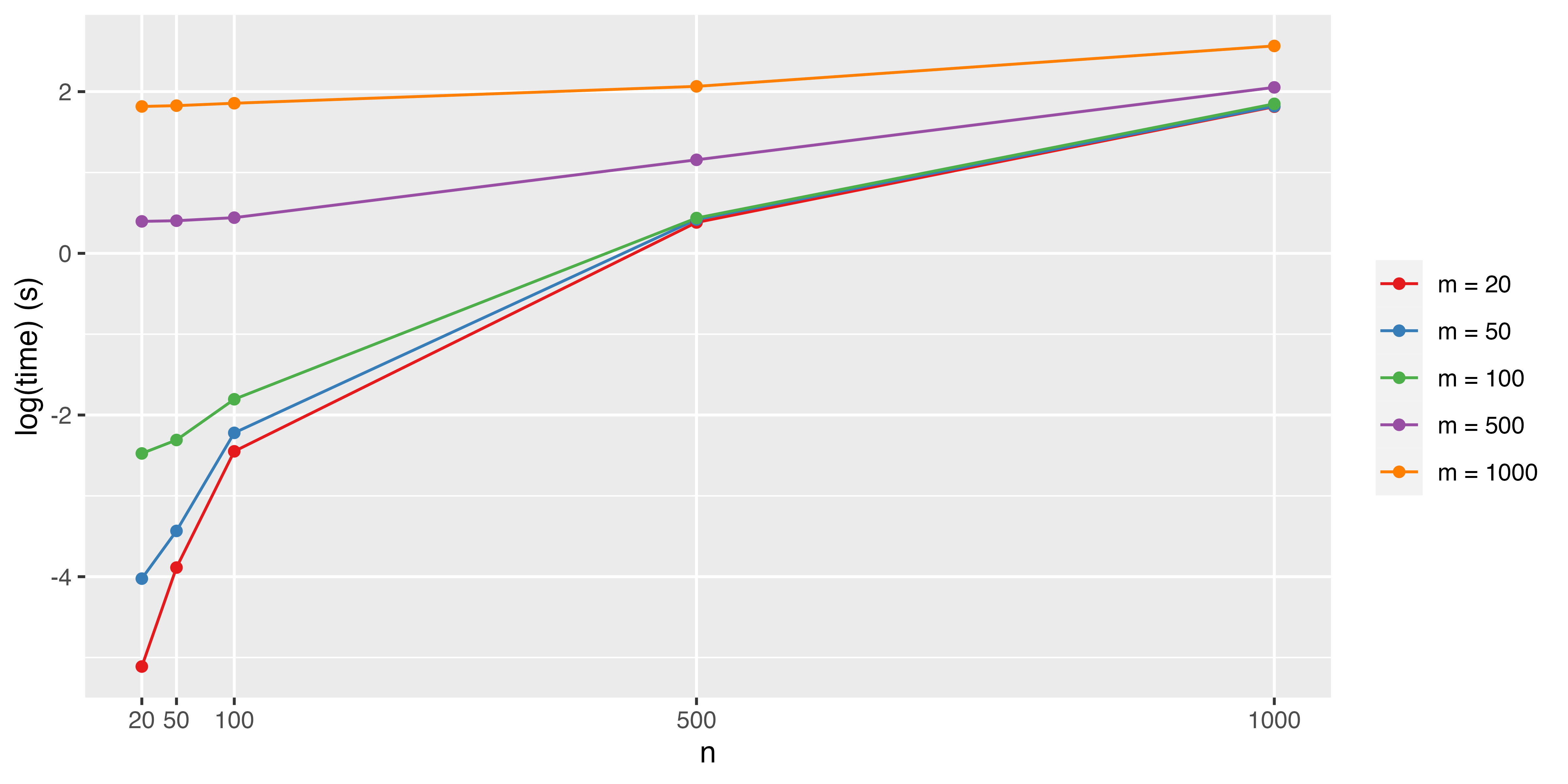
Figure 1: Median log computation time for a single MCMC iteration as a function of sample size $n$ (x-axis) and $m$ (line color).

In spite of these apparent limitations, there are a variety of approaches one could take to reduce the associated computational burdens of this model. The simplest approach would be to parameterize the covariance matrix as $\bm{\Omega}_{i}=\sigma^{2}_{i}\mathbf{C}(\bm{\theta})$ where $\bm{\theta}$ is specified and not estimated (as is done in Section 5): this would remove the Metropolis-Hastings steps required to estimate $\rho_{u,i}$ and $\rho_{v,i}$. Alternatively, one could use a compactly-supported kernel function (see, e.g., Wendland,, 1995; Buhmann,, 2000; Genton,, 2000; Gneiting,, 2002; Melkumyan and Ramos,, 2009) and leverage sparse matrix techniques or, since there is a direct connection between the scaling of our methodology and the scaling of Gaussian processes, one could utilize one of the broad suite of approximate GP methods (see, e.g., Heaton et al.,, 2019). For now, we leave these considerations to future work. Ultimately, these computational challenges are the price for full Bayesian uncertainty quantification for structured orthonormal matrices, and any simplifications or shortcuts should be fully vetted for impacts on the method’s robustness.

4 Synthetic data example

We now conduct a simulation study to illustrate the impact of various parameterizations of the proposed prior with the Bayesian SVD model on basis function and data recovery. For all simulations, the target “true” basis functions $\mathbf{U}$ and $\mathbf{V}$ are simulated according to the generating mechanism described in section 2.1 (e.g., to produce the orthonormal matrix in (1)) with $\bm{\Omega}^{u}_{i}=\sigma^{2}_{u,i}\mathbf{C}_{u}(\bm{\theta}_{u,i})$ and $\bm{\Omega}^{v}_{i}=\sigma^{2}_{v,i}\mathbf{C}_{v}(\bm{\theta}_{v,i})$ where the elements of $\mathbf{C}_{u}(\bm{\theta}_{u,i})$ and $\mathbf{C}_{v}(\bm{\theta}_{v,i})$ are defined by the Matérn correlation function with $\bm{\theta}_{u,i}=(\nu_{u,i},\rho_{u,i})$ and $\bm{\theta}_{v,i}=(\nu_{v,i},\rho_{v,i})$ and the diagonal matrix $\mathbf{D}$ is specified. For all simulations, we specify the true number of basis function $k=5$ with covariance parameters $(\nu_{(\cdot),i},\rho_{(\cdot),i})=(3.5,3)$ for both $\mathbf{U}$ and $\mathbf{V}$ and for all $i=1,\dots,k$, and diagonal matrix $\mathbf{D}=diag(40,30,20,10,5)$.

Data are simulated according to (4) with $\bm{\Sigma}=\sigma^{2}\mathbf{I}_{n}$, $n=100$, $m=100$, $\mathbf{s}_{1},...,\mathbf{s}_{n}$ equally spaced in $\mathcal{S}=[-5,5]$, $t_{1},...,t_{m}$ are equally spaced in $\mathcal{T}=[0,10]$. To determine the effect of measurement error, we generate data sets with $\sigma^{2}$ chosen such that the signal-to-noise ratio (SNR) is $SNR=[10,5,2,1,0.5,0.1]$. Specifically, let $\bm{\eta}$ be a random $n\times m$ matrix of iid standard normal random variables. Then, $\sigma=\sqrt{\frac{var(\mathbf{Y})}{SNR*var(\bm{\eta})}}$, and the simulated data is $\mathbf{Z}=\mathbf{Y}+\sigma\bm{\eta}$ (see the supplement Figure S.2) with $var(\mathbf{Y})/var(\mathbf{Z}-\mathbf{Y})=SNR$. One realization of the simulated data with a SNR of 1 and the $\mathbf{U}$ and $\mathbf{V}$ basis functions are shown in Figure 2.

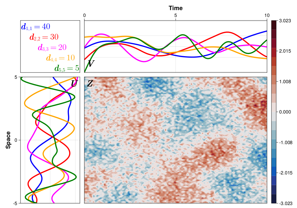
Figure 2: Randomly simulated data $\mathbf{Z}$ (main plot) with a signal-to-noise ratio of 1 and the randomly simulated $\mathbf{U}$ (left) and $\mathbf{V}$ (top) basis functions.

As discussed in Section 3.1.3, using this model only requires specification of $k$, the number of basis functions used in $\mathbf{U}$ and $\mathbf{V}$. To investigate how the number of basis functions impacts model recovery, we estimate the model specifying $k=[3,4,5,6,7]$ (recall the true $k=5$) for each level of SNR. For each SNR and $k$ combination, we obtain $10000$ posterior samples of the model parameters, discarding the first $5000$ as burn-in. To understand the variability in the specification of $k$ and SNR on model recovery, we repeat this process 100 times. Due to the large number of models, convergence was assessed graphically for a random subset of the fits with no issues detected.

For each posterior simulation, we calculated the 95% coverage rate (CR) and root mean square error (RMSE) for $\mathbf{U}$, $\mathbf{V}$, and the “true” surface $\mathbf{Y}=\mathbf{U}\mathbf{D}\mathbf{V}^{\prime}$. If the true $k^{*}$ is greater than the specified $k$, the empirical CR and RMSE are computed only for the first $k$ basis functions and then averaged over the $k$ estimates (e.g., we do not consider the last $k^{*}-k$ basis functions when computing CR and RMSE). If the true $k^{*}$ is less than the specified $k$, the empirical CR and RMSE for the “extra” $k-k^{*}$ basis functions are compared to the zero line and the reported CR and RMSE values are obtained by averaging over the $k$ estimates. Additionally, for each simulation we computed the C-SVD using the base linear algebra library, LinearAlgebra.jl, in Julia (Bezanson et al.,, 2017) and computed the RMSE of the calculated $\mathbf{U},\mathbf{V}$, and reconstructed surface $\mathbf{Y}$ assuming the same truncation value $k$. The coverage rates and the RMSE are shown in Figure 3. The results of one simulation are shown in Figure 4 based on the data shown in Figure 2.

(a) Coverage rate, aggregated across repeated samples

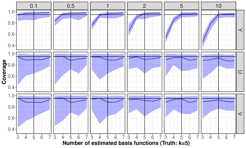
(b) Root mean square error, aggregated across repeated samples

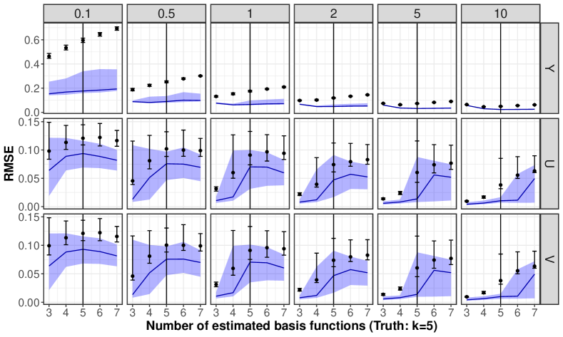
Figure 3: Validation results from the synthetic data example, showing coverage rate (top) and root mean square error (bottom). In each panel, the solid blue line is the median Monte Carlo coverage rate and shaded regions are the 95% Monte Carlo uncertainty bounds for the coverage rate over synthetic replicates. Results are shown for varying levels of SNR and values of $k$ for the recovered surface $\mathbf{Y}$ (top), $\mathbf{U}$ basis functions (middle), and $\mathbf{V}$ basis functions (bottom). The SNR values range from 0.1 (left) to 10 (right). The black vertical line indicates $k=5$ (true $k$ value) and the horizontal black line for (a) is at 95% (the nominal coverage rate). In panel (b), the black point and error bars show the median and 95% bootstrapped confidence interval for the RMSE using the algorithmic C-SVD method.

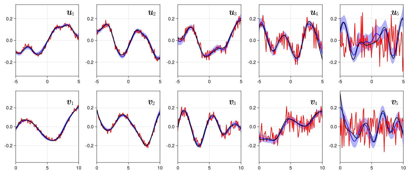
Figure 4: Posterior mean (blue line), 95% credible intervals (shaded blue region), truth (black line), and C-SVD estimate (red line) for the $\mathbf{U}$ and $\mathbf{V}$ basis functions from a random simulation. The data associated with this random simulation is shown in Figure 2.

From Figure 3(a), we see our median coverage rate for the $\mathbf{U}$ (middle row) and $\mathbf{V}$ (bottom row) basis functions (blue line) is near the nominal level (horizontal black line) and the 95% Monte Carlo uncertainty bounds (MCUB) for the coverage rate (blue shaded region) covers the nominal level for all SNR levels and regardless of the specification of $k$. This implies that posterior uncertainties are well calibrated and robust to mis-specifications of the number of estimated basis functions, regardless of the magnitude of the noise. For the recovered data (top row), we see the 95% MCUB cover the nominal level for all SNR levels with $k$ greater than 5. However, for $k$ less than 5, achieving the nominal coverage depends on SNR: in low signal cases (e.g., SNR = 0.1), the uncertainties are well calibrated, while posterior uncertainties are too small (i.e., coverage of the truth is much less than the nominal level) when the signal is stronger (SNR $>$ 0.5). This counterintuitive result is due to the impact of unaccounted signal for higher-order basis functions ($i=4$ and/or $i=5$) on the signal: for large SNR, individual basis functions both (a) contribute more to the overall uncertainty in the data and also (b) have narrower posterior distributions, such that ignoring one or more true basis functions causes the model to underestimate data uncertainties (e.g., see Figure 4). Conversely, for smaller SNR, there is more uncertainty in each basis function estimate and the impact of higher-order basis functions on the estimated surface is reduced, to the extent that the model can recover the nominal coverage of the data.

For the RMSE, shown in Figure 3(b), the most notable result is that the median RMSE for our approach (blue line) is systematically lower than the corresponding RMSE from the algorithmic C-SVD approach for both data (top row) and basis functions (middle and bottom rows), across SNR levels and specification of $k$. In other words, estimates of the basis functions in both $\mathbf{U}$ and $\mathbf{V}$ and the recovered data have systematically lower errors than what one can obtain from the algorithmic approach. Regarding RMSE for estimates of the recovered surface, the median error (blue line) decreases as a function of SNR, as expected, and interestingly the data RMSE is relatively insensitive to specification of $k$. For the $\mathbf{U}$ and $\mathbf{V}$ basis functions (middle and bottom rows, respectively, of Figure 3), we see that trajectories of RMSE estimates for our proposed approach and the C-SVD mirror each other, with our estimates being systematically, but not significantly, lower. However, across SNR levels, the RMSE actually increases as one moves from $k=3$ to $k=7$ (even though the true $k=5$). For SNR equal to 5 and 10, we see a dramatic spike in the RMSE estimate and uncertainty for the $\mathbf{U}$ and $\mathbf{V}$ basis functions for $k=6$ and $7$. This is because we are comparing against the zero line for these cases: while the uncertainty bounds for these basis function covers the zero line (as seen in the coverage results in Figure 3a.), there is a lot of variability in these estimates (with relatively lower uncertainty due to larger signal), leading to inflated RMSE values.

In conclusion, this synthetic data example shows the proposed method has well calibrated uncertainty and significantly reduces the impact of measurement noise on the basis function estimates. However, there is a significant trade-off in choosing $k$ to be too small or large based on the magnitude of the SNR. Based on our simulation, there will be significant bias in the recovered surface but not in the estimated basis functions if $k$ is too small and the SNR is low. Additionally, there will not be significant bias in the recovered surface or in the estimated basis functions if either $k$ is too small and the SNR is large or $k$ is too large. The only trade-off for too large of $k$ are inflated RMSE’s for the extraneous basis function which could lead to underestimated RMSE’s in the recovered surface. Therefore, we suggest erring on the side of choosing $k$ to be too large.

5 Sea surface temperature

As discussed in the introduction, empirical orthogonal functions or EOFs are commonly used in climate sciences to compute (among other things) indices that summarize the modes of large-scale variability in the Earth system. One such index is the Pacific Decadal Oscillation (PDO; Mantua et al.,, 1997). Mathematically speaking, the PDO is defined as the leading EOF of the North Pacific (poleward of 20^∘N) sea-surface temperature (SST) monthly averaged anomalies after the global climatological mean has been removed (see supplement S.5 for specific details). When the PDO has a positive value, the interior SST of the Pacific is anomalously cool and the west coast of the Americas is anomalously warm. Conversely, when the PDO has a negative value, the interior SST of the Pacific is anomalously warm and the coast of the Americas is anomalously cool (Mantua and Hare,, 2002). While it is known that the PDO is highly correlated with other physical climate processes (e.g., the El Niño/Southern Oscillation and the Pacific-North American teleconnection pattern; Newman et al.,, 2016; Risser et al.,, 2021), we ignore these relationships for this example.

We use gridded monthly SST data from the Met Office Hadley Centre (HadISST) at 1^∘ resolution from January 1870 to June 2022 (Rayner,, 2003). The data are detrended according to the process described in the supplement (S.5; derived from Hartmann,, 2015) and we focus on the subset to only include data from 20^∘- 60^∘N and 110^∘- 280^∘E for a total of 4267 spatial locations across 1830 time points. While it is possible to create a design matrix that is equivalent to the detrending step and incorporate the matrix into the model structure through $\mathbf{M}$ in (3), this would have resulted in a substantial number of parameters to estimate. Therefore, we detrend the data a priori to parameter estimation. The detrended data is shown in the supplement (Figure S.3) along with the first EOF and the PDO index time series as computed using C-SVD.

Our goal is to understand the uncertainty in the PDO index when the spatial basis functions are modeled dependently. However, we do not want to impose temporal dependence on the PDO index: in climate science applications that utilize the index (e.g. Zhang et al.,, 2010), one is typically interested in the month-to-month variability of the index. Therefore, we parameterize the covariance matrix for the prior of the spatial basis functions using the Matérn kernel with $\rho=560$km and $\nu=3.5$ and the covariance matrix for the prior of the temporal basis functions using the identity matrix. The effective range $\rho=560$km is chosen based on empirical variogram estimates. Last, while our interest is only on the leading basis function, we specify $k=5$ so that the estimate of the leading basis function is not biased by failure to account for the lower order signals. We obtain $10000$ samples from the posterior, discarding the first $5000$ as burn-in, where convergence is assessed graphically with no issues detected.

The posterior samples of the PDO (P-PDO) index from January 2010 to June 2022 are shown in Figure 5 c), where the black line indicates the posterior mean and the yellow shaded region is the 95% CI. The P-PDO index preserves the general structure of the PDO index (Figure 5 a)), which is to be expected as the PDO signal has been shown to be robust to the data source (e.g., HadISST, COBE, ERSST, Kaplan) and sample period (e.g., analysis of different time periods; Newman et al.,, 2016). To further support this claim, we found no significant departure between the P-PDO and PDO index based on the 95% CI (Figure 5 e)). As was expected, the posterior mean of the leading spatial EOF (Figure 5 d); P-EOF) is smoother than the algorithmic estimate of the leading spatial EOF as seen by observing the difference in individual contours (Figure 5 b); A-EOF), but the general spatial structure is the same. The posterior difference between the P-EOF and A-EOF (Figure 5 f)) highlights areas where the P-EOF is smoother than the A-EOF estimate, with the most visually apparent being in the spatial region of 30^∘- 45^∘N and 153^∘- 129^∘W, corresponding to the transition from a positive to negative value. Interestingly, we see a “banding” pattern in the difference plot which is due to the P-EOF values smoothing the rougher estimates of the A-EOF values - effectively bisecting the A-EOF values.

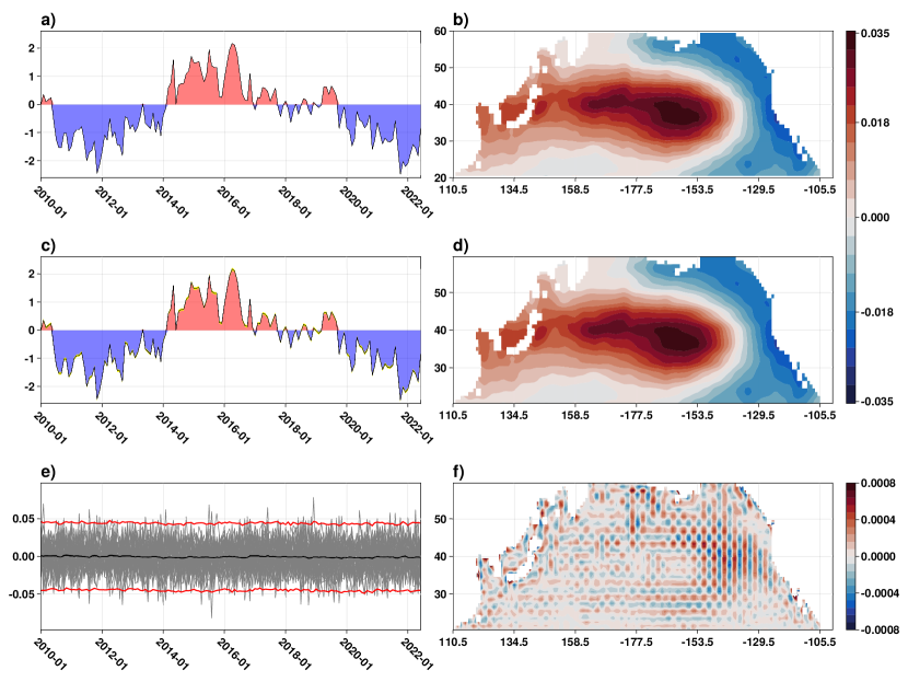
Figure 5: a) Algorithmic PDO index from January 2010 to June 2022, b) leading spatial EOF c) posterior mean (black) and 95% CI (yellow shaded region) for the PDO index January 2010 to June 2022, d) posterior mean of the leading spatial EOF, e) mean posterior difference between the posterior draws from the P-PDO and the A-PDO index (black line) along with 95% difference CI (red lines) and 50 random realizations of the difference (gray lines), f) posterior difference between the Bayesian estimate and the algorithmic estimate for the leading spatial EOF where red (blue) signifies the Bayesian estimate is larger (smaller) than the algorithmic estimate.

In effect, our Bayesian estimate samples from the distribution of the PDO index while accounting for the measurement error in the SST data and the spatial dependence present in the spatial basis functions under the model assumptions used to generate the HadISST gridded data product. The primary benefit of using a Bayesian approach to modeling the PDO index is now apparent: posterior draws of the spatial basis functions, together with posterior draws of all other hyperparameters, imply a posterior distribution over the PDO index itself. While this may seem like an obvious statistical conclusion, this is a nontrivial result: we have now generated an observational “ensemble” of a dominant mode of climate variability (instead of just a central estimate with standard errors). The members of this ensemble (the different realizations of the PDO index calculated from each posterior draw) can be plugged into an analysis such as Zhang et al., (2010), providing a straightforward way to propagate uncertainty in the PDO index through to the resulting scientific conclusions (potentially obviating challenges associated with error-in-variable regression approaches). Importantly, as the output of a statistical model, this observational ensemble of PDO estimates is calculated at considerably less computational cost than other approaches to generating observational ensembles (e.g., the ensemble component of ERA5, Hersbach et al.,, 2020).

6 Discussion

We proposed a novel prior distribution for structured orthonormal matrices that is an extension of Hoff, (2007), where the basis functions are able to be modeled dependently. The prior is based on the projected normal distribution which we augment with a latent length. When our prior is combined with a normal data model, the resulting full conditional distributions for the basis functions are conjugate, resulting in analytically straightforward MCMC sampling. We describe how the prior can be used to conduct posterior inference on a general class of probabilistic SVD models and how to extend the proposed model to various other applications. We discussed various mathematical properties of our probabilistic SVD model (supplement S.2) and illustrated its capability through a simulation study. The model is then used to draw inference on the PDO index, an important metric for characterizing the state of Earth’s climate.

The synthetic data examples and real world example presented in Sections 4 and 5, respectively, all highlighted the model’s efficacy on gridded data. However, the model is equally well suited for non-uniformly spaced data so long as the spacing is consistent within space and within time. If the data are not spaced consistently within space and within time, this would constitute a missing data problem, which we plan to explore in future work.

Another area for possible extension relies on computational improvements. For all synthetic data examples and the real world example, we relied on the support of a super computer. While each individual model combination in Section 4 could be run on a personal computer, the overall simulation in Section 4 as well as the real world example in Section 5 were impractical for a personal computer due to the time demand. As discussed in Section 3.3, this is because each iteration of the MCMC algorithm requires the inversion of $\mathbf{N}^{u\,\prime}_{i}\bm{\Omega}^{u}_{i}\mathbf{N}^{u}_{i}$ and $\mathbf{N}^{v\,\prime}_{i}\bm{\Omega}^{v}_{i}\mathbf{N}^{v}_{i}$ for $i=1,...,k$ in addition to the Metropolis-Hastings step required to estimate $\rho_{u,i}$ and $\rho_{v,i}$. While possible to run on a personal computer from a memory stand-point, the amount of time required to run the simulation and real world example is the impractical aspect. Computational work focusing on improving the speed of this calculation would prove beneficial for model feasibility. For example, using sparse kernels, which have favorable computational properties for large data sets (Noack et al.,, 2023), can be used to reduce the computational burden present with dense matrices.

The choice of $k$, the number of basis functions, is the only major subjective choice in our proposed probabilistic SVD model. While we show the mis-specification of $k$ does not have a negative impact when erring on the side of $k$ being too large, a more flexible model estimating $k$ is attractive. To estimate $k$, Hoff, (2007) proposed a variable-rank model utilizing the so-called spike-and-slab variable selection prior (Mitchell and Beauchamp,, 1988). However, because of the difference in our prior compared to the prior proposed by Hoff, (2007), incorporating the spike-and-slab prior into our proposed model would require extra theoretical work. Work focused on estimating the rank $k$ with our framework would produce a very flexible approach for modeling spatio-temporal random effects.

A Appendix

A.1 Proofs of propositions

We now prove the propositions describing the properties of the orthogonal matrix constructed in section 2.1.

 

Proposition 1. The matrix $\mathbf{W}=\mathbf{X}(\mathbf{X}^{\prime}\mathbf{X})^{-1/2}$ is invariant to right-orthogonal transformation. That is, for $\mathbf{H}:\mathbb{R}^{k}\rightarrow\mathbb{R}^{k}$ an orthogonal transformation matrix, $\mathbf{W}\mathbf{H}\overset{d}{=}\mathbf{W}$.

Proof.

From Corollary 2.4.7 of Chikuse, (2003), the distribution of $\mathbf{W}$ is invariant to right-orthogonal transformation if

• $\mathbf{X}$ is an $n\times k$ matrix that is invariant to right-orthogonal transformation and

• the density of $\mathbf{X}$ has the form

  $$f_{X}(X)=|\bm{\Sigma}|^{-k/2}g(\mathbf{X}^{\prime}\bm{\Sigma}^{-1}\mathbf{X}),$$

  with $\bm{\Sigma}$ a positive-definite matrix.

First, for $\mathbf{X}_{i},i=1,...,K$, we show invariance to right-orthogonal transformation by induction. Let $\mathbf{H}_{i}:\mathbb{R}^{i}\rightarrow\mathbb{R}^{i}$ be an orthogonal transformation.

1. For $i=1$, $\mathbf{X}_{1}\mathbf{H}_{1}=\mathbf{x}_{1}\mathbf{H}_{1}\overset{d}{=}\mathbf{x}_{1}=\mathbf{X}_{1}$.

2. Assume for $i=j$, $\mathbf{X}_{j}\mathbf{H}_{j}|\mathbf{X}_{j-1}\overset{d}{=}\mathbf{X}_{j}|\mathbf{X}_{j-1}$.

3. By the characteristic function of $\mathbf{X}_{j+1}\mathbf{H}_{j+1}=\mathbf{X}_{j+1}^{\star}$, we have

   $$\varphi(\mathbf{X}_{j+1}\mathbf{H}_{j+1}|\mathbf{X}_{j}) =E\left[\left.\exp\left\{i\sum_{\ell=1}^{j+1}\mathbf{t}_{\ell}^{\prime}\mathbf{x}_{\ell}^{\star}\right\}\right|\mathbf{X}_{j}\right]$$

   $$=\exp\left\{i\sum_{\ell=1}^{j}\mathbf{t}_{\ell}^{\prime}\mathbf{x}_{\ell}^{\star}\right\}E\left[\exp\left\{i\mathbf{t}_{j+1}^{\prime}\mathbf{x}_{j+1}^{\star}\right\}|\mathbf{X}_{j}\right],$$

   where $\mathbf{t}_{j+1}^{\prime}\mathbf{x}_{j+1}^{\star}=\mathbf{t}_{j+1}^{\prime}\mathbf{P}_{j}^{\star}\mathbf{z}_{j+1}$, $\mathbf{P}_{j}^{\star}=\mathbf{I}-(\mathbf{X}_{j}\mathbf{H}_{j})((\mathbf{X}_{j}\mathbf{H}_{j})^{\prime}(\mathbf{X}_{j}\mathbf{H}_{j}))^{-1}(\mathbf{X}_{j}\mathbf{H}_{j})^{\prime}$, and $\mathbf{z}_{j+1}\sim N_{n}(\bm{0},\bm{\Omega}_{j})$ is independent of $\mathbf{X}_{j}$. We also have

   $$\mathbf{P}_{j}^{\star} =\mathbf{I}-(\mathbf{X}_{j}\mathbf{H}_{j})\{(\mathbf{X}_{j}\mathbf{H}_{j})^{\prime}(\mathbf{X}_{j}\mathbf{H}_{j})\}^{-1}(\mathbf{X}_{j}\mathbf{H}_{j})^{\prime}$$

   $$=\mathbf{I}-\mathbf{X}_{j}\mathbf{H}_{j}\mathbf{H}_{j}^{-1}(^{\prime}\mathbf{X}_{j}^{\prime}\mathbf{X}_{j})^{-1}\mathbf{H}_{j}^{\,\prime-1}\mathbf{H}_{j}^{\prime}\mathbf{X}_{j}$$

   $$=\mathbf{I}-\mathbf{X}_{j}(\mathbf{X}_{j}^{\prime}\mathbf{X}_{j})^{-1}\mathbf{X}_{j}$$

   $$=\mathbf{P}_{j}.$$

   Therefore, the characteristic function is

   $$\varphi(\mathbf{X}_{j+1}\mathbf{H}_{j+1}|\mathbf{X}_{j}) =\exp\left\{i\sum_{\ell=1}^{j}\mathbf{t}_{\ell}^{\prime}\mathbf{x}_{\ell}^{\star}\right\}E\left[\exp\left\{i\mathbf{t}_{j+1}^{\prime}\mathbf{P}_{j}^{\star}\mathbf{z}_{j+1}\right\}|\mathbf{X}_{j}\right]$$

   $$=\exp\left\{i\sum_{\ell=1}^{j}\mathbf{t}_{\ell}^{\prime}\mathbf{x}_{\ell}^{\star}\right\}\exp\left\{-\frac{1}{2}\mathbf{t}_{j+1}^{\prime}\mathbf{P}_{j}^{\star}\bm{\Omega}_{j}\mathbf{P}_{j}^{\,\prime\star}\mathbf{t}_{j+1}\right\}$$

   $$=\exp\left\{i\sum_{\ell=1}^{j}\mathbf{t}_{\ell}^{\prime}\mathbf{x}_{\ell}^{\star}\right\}\exp\left\{-\frac{1}{2}\mathbf{t}_{j+1}^{\prime}\mathbf{P}_{j}\bm{\Omega}_{j}\mathbf{P}_{j}^{\,\prime}\mathbf{t}_{j+1}\right\}.$$ (A.1)

   Similarly, the characteristic function for $\mathbf{X}_{j+1}$ is

   $$\varphi(\mathbf{X}_{j+1}|\mathbf{X}_{j})=\exp\left\{i\sum_{\ell=1}^{j}\mathbf{t}_{\ell}^{\prime}\mathbf{x}_{\ell}\right\}\exp\left\{-\frac{1}{2}\mathbf{t}_{j+1}^{\prime}\mathbf{P}_{j}\bm{\Omega}_{j}\mathbf{P}_{j}^{\,\prime}\mathbf{t}_{j+1}\right\}.$$ (A.2)

   By assumption, $\mathbf{X}_{j}\mathbf{H}_{j}\overset{d}{=}\mathbf{X}_{j}$, so $\{\mathbf{x}_{1}^{\star},...,\mathbf{x}_{j}^{\star},\mathbf{P}_{j}^{\star}\}\overset{d}{=}\{\mathbf{x}_{1},...,\mathbf{x}_{j},\mathbf{P}_{j}\}$ and the characteristic function (3) and (A.2) are equal. Because the characteristic functions specify the distributions, $\mathbf{X}_{j+1}\mathbf{H}_{j+1}\overset{d}{=}\mathbf{X}_{j+1}$.

Next, we show the density of $\mathbf{X}$ is of the form

$$f_{\mathbf{X}}(\mathbf{X})=|\bm{\Sigma}|^{-k/2}g(\mathbf{X}^{\prime}\bm{\Sigma}^{-1}\mathbf{X})$$

using induction.

1. For $i=1$, $\mathbf{X}_{1}=\mathbf{x}_{1}$ and

   $$f_{\mathbf{x}_{1}}(\mathbf{x}_{1})\propto|\bm{\Omega}_{1}|^{-1/2}g(\mathbf{x}_{1}^{\prime}\bm{\Omega}_{1}^{-1}\mathbf{x}_{1}).$$

2. For $i=2$, $f_{\mathbf{x}_{2}|\mathbf{X}_{1}}(\mathbf{x}_{2}|\mathbf{X}_{1})\sim N(\bm{0},\mathbf{P}_{1}\bm{\Omega}_{2}\mathbf{P}_{1}^{\prime})$. Taking the Schur complement, $\mathbf{P}_{1}\bm{\Omega}_{2}\mathbf{P}_{1}^{\prime}=\bm{\Sigma}_{11}-\bm{\Sigma}_{12}\bm{\Sigma}_{22}^{-1}\bm{\Sigma}_{21}$ and the joint distribution is

   $$\begin{bmatrix}\mathbf{x}_{1}\\ \mathbf{x}_{2}\end{bmatrix}\sim N\left(\bm{0},\begin{bmatrix}\bm{\Sigma}_{11}&\bm{\Sigma}_{12}\\ \bm{\Sigma}_{21}&\bm{\Sigma}_{22}\\ \end{bmatrix}\right).$$

   From known properties of the multivariate normal and the matrix normal, $[\mathbf{x}_{1},\mathbf{x}_{2}]\equiv\mathbf{X}_{2}\sim MN_{n\times 2}(\bm{0},\mathbf{A},\mathbf{B})$ where

   $$\begin{bmatrix}\bm{\Sigma}_{11}&\bm{\Sigma}_{12}\\ \bm{\Sigma}_{21}&\bm{\Sigma}_{22}\\ \end{bmatrix}=\mathbf{B}\otimes\mathbf{A},$$

   where $\mathbf{A}\in\mathbb{R}^{2\times 2}$, $\mathbf{B}\in\mathbb{R}^{n\times n}$. Also, because $\mathbf{B}\otimes\mathbf{A}$ is invertible, $(\mathbf{B}\otimes\mathbf{A})^{-1}=\mathbf{B}^{-1}\otimes\mathbf{A}^{-1}$ and both $\mathbf{A}$ and $\mathbf{B}$ are invertible. Thus,

   $$f_{\mathbf{X}_{2}}(\mathbf{X}_{2})\propto|\mathbf{B}|^{-1/2}g(\mathbf{X}_{2}^{\prime}\mathbf{B}^{-1}\mathbf{X}_{2}).$$

3. For $i=j$, $f_{\mathbf{x}_{j}|\mathbf{X}_{j-1}}(\mathbf{x}_{j}|\mathbf{X}_{j-1})\sim N(\bm{0},\mathbf{P}_{j-1}\bm{\Omega}_{j}\mathbf{P}_{j-1}^{\prime})$, where the Schur complement is $\mathbf{P}_{j-1}\bm{\Omega}_{j}\mathbf{P}_{j-1}^{\prime}=\bm{\Sigma}_{11}-\bm{\Sigma}_{12}\bm{\Sigma}_{22}^{-1}\bm{\Sigma}_{21}$. The joint distribution

   $$\begin{bmatrix}\mathbf{X}_{j-1}\\ \mathbf{x}_{j}\end{bmatrix}\sim N\left(\bm{0},\begin{bmatrix}\bm{\Sigma}_{11}&\bm{\Sigma}_{12}\\ \bm{\Sigma}_{21}&\bm{\Sigma}_{22}\\ \end{bmatrix}\right)$$

   can be written as a matrix normal $[\mathbf{X}_{j-1},\mathbf{x}_{j}]\equiv\mathbf{X}_{j}\sim MN_{n\times j}(\bm{0},\mathbf{A},\mathbf{B})$ where

   $$\begin{bmatrix}\bm{\Sigma}_{11}&\bm{\Sigma}_{12}\\ \bm{\Sigma}_{21}&\bm{\Sigma}_{22}\\ \end{bmatrix}=\mathbf{B}\otimes\mathbf{A}$$

   with

   $$f_{\mathbf{X}_{j}}(\mathbf{X}_{j})\propto|\mathbf{B}|^{-1/2}g(\mathbf{X}_{j}^{\prime}\mathbf{B}^{-1}\mathbf{X}_{j}).$$

Therefore, the density of $\mathbf{X}$ is of the form

$$f_{\mathbf{X}}(\mathbf{X})=|\bm{\Sigma}|^{-k/2}g(\mathbf{X}^{\prime}\bm{\Sigma}^{-1}\mathbf{X}).$$

∎

 

Proposition 2. $\mathbf{w}_{i}|\mathbf{W}_{i-1}\overset{d}{=}\mathbf{N}_{i-1}\widetilde{\mathbf{w}}_{i}|\mathbf{W}_{i-1}$ where the columns of $\mathbf{N}_{i-1}$ form an orthonormal basis for the null space of $\mathbf{W}_{i-1}$ and $\widetilde{\mathbf{w}}_{i}|\mathbf{W}_{i-1}\sim PN_{n-i+1}(\bm{0},\mathbf{N}_{i-1}^{\prime}\bm{\Omega}_{i}\mathbf{N}_{i-1})$ is the projected weight function.

Proof.

The following argument is similar to Hoff, (2007), except now we account for dependence structure and the resulting distribution is different. By construction, $\mathbf{w}_{i}=\mathbf{P}_{i-1}\mathbf{z}_{i}/(\mathbf{z}_{i}^{\prime}\mathbf{P}_{i-1}^{\prime}\mathbf{P}_{i-1}\mathbf{z}_{i})^{1/2}$ where $\mathbf{P}_{i-1}$ has $n-i+1$ eigenvalues equal to 1 and the rest being 0. Let the eigenvalue decomposition be $\mathbf{P}_{i-1}=\mathbf{N}_{i-1}\mathbf{N}_{i-1}^{\prime}$ where $\mathbf{N}_{i-1}$ is an $n\times(n-i+1)$ matrix whose columns span the null space of $\mathbf{W}_{i}$. Making the substitution $\mathbf{P}_{i-1}=\mathbf{N}_{i-1}\mathbf{N}_{i-1}^{\prime}$,

$$\mathbf{w}_{i} =\frac{\mathbf{P}_{i-1}\mathbf{z}_{i}}{(\mathbf{z}_{i}^{\prime}\mathbf{P}_{i-1}^{\prime}\mathbf{P}_{i-1}\mathbf{z}_{i})^{1/2}}$$

$$=\frac{\mathbf{N}_{i-1}\mathbf{N}_{i-1}^{\prime}\mathbf{z}_{i}}{(\mathbf{z}_{i}^{\prime}\mathbf{N}_{i-1}^{\prime}\mathbf{N}_{i-1}\mathbf{N}_{i-1}\mathbf{N}_{i-1}^{\prime}\mathbf{z}_{i})^{1/2}}$$

$$=\mathbf{N}_{i-1}\frac{\mathbf{N}_{i-1}^{\prime}\mathbf{z}_{i}}{(\mathbf{z}_{i}^{\prime}\mathbf{N}_{i-1}\mathbf{N}_{i-1}^{\prime}\mathbf{z}_{i})^{1/2}}.$$

Note that $\mathbf{P}_{i-1}=\mathbf{I}-\mathbf{W}_{i-1}\mathbf{W}_{i-1}^{\prime}$, so $\mathbf{w}_{i}|\mathbf{W}_{i-1}\overset{d}{=}\mathbf{N}_{i-1}\frac{\mathbf{N}_{i-1}^{\prime}\mathbf{z}_{i}}{(\mathbf{z}_{i}^{\prime}\mathbf{N}_{i-1}\mathbf{N}_{i-1}^{\prime}\mathbf{z}_{i})^{1/2}}$. Because $\mathbf{z}_{i}\sim N_{n}(\bm{0},\bm{\Omega}_{i})$, we have $\mathbf{N}_{i-1}^{\prime}\mathbf{z}_{i}|\mathbf{W}_{i-1}\sim N_{n}(\bm{0},\mathbf{N}_{i-1}^{\prime}\bm{\Omega}_{i}\mathbf{N}_{i-1})$ and $\frac{\mathbf{N}_{i-1}^{\prime}\mathbf{z}_{i}}{(\mathbf{z}_{i}^{\prime}\mathbf{N}_{i-1}\mathbf{N}_{i-1}^{\prime}\mathbf{z}_{i})^{1/2}}\equiv\widetilde{\mathbf{w}}_{i}|\mathbf{W}_{i-1}\sim PN(\bm{0},\mathbf{N}_{i-1}^{\prime}\bm{\Omega}_{i}\mathbf{N}_{i-1})$. ∎

S Supplemental Material

S.1 Full conditional distributions

The diagonal matrix $\mathbf{D}$ and the length-scale parameters $\rho_{u,i}$ and $\rho_{v,i}$ do not have conjugate updates and so we use a Metropolis-within-Gibbs step to estimate these parameters. For all Metropolis steps, we use a truncated normal for the proposal distribution with the mean set to the most recently accepted value. For $\mathbf{D}$ the upper truncation bound is set to infinity and for $\rho_{u,i}$ and $\rho_{v,i}$ the upper truncation bound is set to the max distance for $\mathbf{U}$ (e.g., greatest distance between spatial locations) and $\mathbf{V}$ (e.g., greatest span between time points) divided by 2, respectively. Because the variance of the proposal can influence the acceptance rate, we automatically tune the proposal variance for each parameter individually such that the acceptance rate is between 25% and 45%.

Sampling Algorithm

For each iteration of the MCMC algorithm, do:

1. Update $\mathbf{D}$ using a Metropolis step

2. For $i\in\{1,...,k\}$ update $\mathbf{u}_{i}|\mathbf{U}_{-i}\overset{d}{=}\mathbf{N}^{u}_{i}\widetilde{\mathbf{u}}_{i}$ where $\widetilde{\mathbf{u}}_{i}$

   $$[\widetilde{\mathbf{u}}_{i}|\cdot] \sim N(\mathbf{S}_{u}^{-1}\mathbf{m}_{u},\mathbf{S}_{u}^{-1})\mathbb{I}(\widetilde{\mathbf{u}}_{i}\in\mathcal{V}_{1,n})$$

   $$\mathbf{m}_{u}=d_{i}\mathbf{N}_{i}^{u\,\prime}\bm{\Sigma}^{-1}\mathbf{E}_{i}\mathbf{v}_{i}$$

   $$\mathbf{S}_{u}=d_{i}^{2}(\mathbf{N}^{u\,\prime}_{i}\bm{\Omega}^{u}_{i}\mathbf{N}^{u}_{i})^{-1}+d_{i}^{2}\mathbf{N}_{i}^{u\,\prime}\bm{\Sigma}^{-1}\mathbf{N}_{i}^{u}.$$

3. For $i\in\{1,...,k\}$ update $\mathbf{v}_{i}|\mathbf{V}_{-i}\overset{d}{=}\mathbf{N}^{v}_{i}\widetilde{\mathbf{v}}_{i}$ where $\widetilde{\mathbf{v}}_{i}$

   $$[\widetilde{\mathbf{v}}_{i}|\cdot] \sim N(\mathbf{S}_{v}^{-1}\mathbf{m}_{v},\mathbf{S}_{v}^{-1})\mathbb{I}(\widetilde{\mathbf{v}}_{i}\in\mathcal{V}_{1,m})$$

   $$\mathbf{m}_{v}=d_{i}\mathbf{N}_{i}^{v\,\prime}\mathbf{E}_{i}^{\prime}\bm{\Sigma}^{-1}\mathbf{u}_{i}$$

   $$\mathbf{S}_{v}=d_{i}^{2}(\mathbf{N}^{v\,\prime}_{i}\bm{\Omega}^{v}_{i}\mathbf{N}^{v}_{i})^{-1}+d_{i}^{2}\mathbf{u}_{i}^{\prime}\bm{\Sigma}^{-1}\mathbf{u}_{i}\mathbf{I}_{m}.$$

4. Recall, we parameterize $\bm{\Sigma}=\sigma^{2}\mathbf{I}_{n}$. The full conditional distribution for $\sigma^{2}$ is

   $$[a|\cdot] \sim IG((\xi+1)(2),(1/A^{2})+\xi/\sigma)$$

   $$[\sigma^{2}|\cdot] \sim IG((nm+\xi)/2,\xi/a+(\mathbf{Z}-\mathbf{U}\mathbf{D}\mathbf{V}^{\prime})^{\prime}(\mathbf{Z}-\mathbf{U}\mathbf{D}\mathbf{V}^{\prime})/2).$$

   We specify $\xi=1$ and $A=10^{5}$ which corresponds to the prior $\sigma\sim\mbox{Half-}t(\xi,A)\equiv\mbox{Half-cauchy}(A)$.

5. Recall, we parameterize $\bm{\Omega}_{u}(\theta_{u,i})=\sigma^{2}_{u,i}\mathbf{C}_{u}(\theta_{u,i})$. For $i\in\{1,...,k\}$ update $\sigma^{2}_{u,i}$ from

   $$[a_{u,i}|\cdot] \sim IG((\xi+1)(2),(1/A^{2})+\xi/\sigma_{u,i})$$

   $$[\sigma^{2}_{u,i}|\cdot] \sim IG((n-k+1+\xi)/2,\xi/a_{u,i}+(d_{i}^{2}\widetilde{\mathbf{u}}_{i}^{\prime}(\mathbf{N}^{u\,\prime}_{i}\bm{\Omega}^{u}_{i}\mathbf{N}^{u}_{i})^{-1}\widetilde{\mathbf{u}}_{i})/2),$$

   with $\xi=1$ and $A=10^{5}$.

6. Recall, we parameterize $\bm{\Omega}_{v}(\theta_{v,i})=\sigma^{2}_{v,i}\mathbf{C}_{v}(\theta_{v,i})$. For $i\in\{1,...,k\}$ update $\sigma^{2}_{v,i}$ from

   $$[a_{v,i}|\cdot] \sim IG((\xi+1)(2),(1/A^{2})+\xi/\sigma_{v,i})$$

   $$[\sigma^{2}_{v,i}|\cdot] \sim IG((m-k+1+\xi)/2,\xi/a_{v,i}+(d_{i}^{2}\widetilde{\mathbf{v}}_{i}^{\prime}(\mathbf{N}^{v\,\prime}_{i}\bm{\Omega}^{v}_{i}\mathbf{N}^{v}_{i})^{-1}\widetilde{\mathbf{v}}_{i})/2),$$

   with $\xi=1$ and $A=10^{5}$.

7. For $i\in\{1,...,k\}$ update $\rho^{2}_{u,i}$ using a Metropolis step

8. For $i\in\{1,...,k\}$ update $\rho^{2}_{v,i}$ using a Metropolis step

S.2 Identity correlation

When $\bm{\Omega}_{i}=\mathbf{I}_{n}$, $\widetilde{\mathbf{w}}_{k}$ in proposition 2 is uniformly distributed on the Stiefel manifold. To see this, note that for $\mathbf{z}_{k}\sim N(0,\mathbf{I})$, $\mathbf{N}_{k-1}^{\prime}\mathbf{z}_{k}\sim N_{n-k+1}(0,\mathbf{I})$, and $\frac{\mathbf{N}_{k-1}^{\prime}\mathbf{z}_{k}}{(\mathbf{z}_{i}^{\prime}\mathbf{N}_{i-1}\mathbf{N}_{i-1}^{\prime}\mathbf{z}_{i})^{1/2}}$ is uniformly distributed on the $n-k+1$ sphere. Also, we see proposition 1 is now equivalent to Hoff, (2007), and $\mathbf{W}$ is the uniform probability measure on $\mathcal{V}_{k,n}$.

The resulting full conditional distributions for $\widetilde{\mathbf{u}}_{i}$ and $\widetilde{\mathbf{v}}_{i}$ when $\bm{\Omega}^{u}_{i}=\mathbf{I}_{n}$ and $\bm{\Omega}^{v}_{i}=\mathbf{I}_{m}$ for the SVD model in S.1 become the von-Mises Fisher distribution, which is equivalent to the full conditionals of Hoff, (2007). To see this, note the mean of $[\widetilde{\mathbf{u}}_{i}|\cdot]$ is $\mathbf{S}_{u}^{-1}\mathbf{m}_{u}=\frac{1}{\sigma^{2}+1}\frac{1}{d_{i}}\mathbf{N}_{i}^{u\,\prime}\mathbf{E}_{i}\mathbf{v}_{i}$ and the covariance is $\mathbf{S}_{u}^{-1}=\left(d_{i}^{2}+\frac{d_{i}^{2}}{\sigma^{2}}\right)^{-1}$. The full conditional distribution

$$[\widetilde{\mathbf{u}}_{i}|\cdot] \propto\exp\left\{-\frac{1}{2}tr\left[-2\widetilde{\mathbf{u}}^{\prime}_{i}d_{i}\mathbf{N}_{i}^{u\,\prime}\mathbf{E}_{i}\mathbf{v}_{i}\left(\frac{1}{\sigma^{2}+1}+\frac{1}{\sigma^{4}+\sigma^{2}}\right)\right]\right\}$$

$$=\exp\left\{-\frac{1}{2}tr\left[-2\widetilde{\mathbf{u}}^{\prime}_{i}d_{i}\mathbf{N}_{i}^{u\,\prime}\mathbf{E}_{i}\mathbf{v}_{i}\left(\frac{1}{\sigma^{2}}\right)\right]\right\},$$

which is the kernel of the von-Mises Fisher distribution. The same result holds for $\widetilde{\mathbf{v}}_{i}$.

S.2.1 Relationship to algorithmic SVD

Computing the SVD of $\mathbf{Y}$,

$$\mathbf{Y} =\mathbf{U}\mathbf{D}\mathbf{V}^{\prime}$$

$$\mathbf{Y} =\mathbf{U}_{-i}\mathbf{D}_{-i}\mathbf{V}^{\prime}_{-i}+d_{i}\mathbf{u}_{i}\mathbf{v}^{\prime}_{i}$$

$$\mathbf{Y}-\mathbf{U}_{-i}\mathbf{D}_{-i}\mathbf{V}^{\prime}_{-i} =\mathbf{E}_{-i}=d_{i}\mathbf{u}_{i}\mathbf{v}^{\prime}_{i}$$

$$\frac{1}{d_{i}}\mathbf{E}_{-i}\mathbf{v}_{i} =\mathbf{u}_{i},$$

so the $i$th basis function can be expressed as a function of the data and other basis functions. The mean of the full conditional distribution $[\widetilde{\mathbf{u}}_{i}|\cdot]$ is $\mathbf{S}_{u}^{-1}\mathbf{m}_{u}=\frac{1}{\sigma^{2}+1}\frac{1}{d_{i}}\mathbf{N}_{i}^{u\,\prime}\mathbf{E}_{i}\mathbf{v}_{i}$, and $E[\widetilde{\mathbf{u}}_{i}|\cdot]\rightarrow\frac{1}{d_{i}}\mathbf{N}_{i}^{u\,\prime}\mathbf{E}_{i}\mathbf{v}_{i}$ as $\sigma^{2}\rightarrow 0$. Mapping to the original space, $\mathbf{N}_{i}^{u}E[\widetilde{\mathbf{u}}_{i}|\cdot]=\frac{1}{d_{i}}\mathbf{N}_{i}^{u}\mathbf{N}_{i}^{u\,\prime}\mathbf{E}_{i}\mathbf{v}_{i}=\frac{1}{d_{i}}\mathbf{E}_{i}\mathbf{v}_{i}$. While not shown here, the same argument applies for $\mathbf{V}$. Therefore, when the covariance is taken to be the identity matrix, the posterior mean of the basis functions is equivalent to the C-SVD basis functions.

To see the relationship visually, we repeat one of the simulation conducted in Section 4 with $SNR=5$, $k=5$, and set the correlation matrices $\mathbf{C}_{u}$ and $\mathbf{C}_{v}$ to be the identity. Here, we still estimate the basis function specific variance $\sigma^{2}_{u,i}$ and $\sigma^{2}_{v,i}$. We obtain 10000 samples from the posterior, discarding the first 5000 as burnin. The resulting estimates for the $\mathbf{U}$ and $\mathbf{V}$ basis functions are shown in Figure S.1, where the posterior mean of the basis functions (blue) is nearly identical to the C-SVD estimates (red). In all cases, we see the 95% intervals (blue shaded region) cover the C-SVD estimates but has  95% coverage of the true line (black).

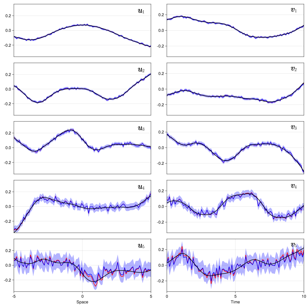
Figure S.1: Posterior mean (blue line), 95% credible intervals (shaded blue region), truth (black line), and C-SVD estimate (red line) for the $\mathbf{U}$ and $\mathbf{V}$ basis function.

S.3 Projected normal distribution

Let $\mathbf{z}_{j}\sim N_{n}(\bm{0},\bm{\Omega}),j=1,...,K$ and $\mathbf{Z}=[\mathbf{z}_{1},...,\mathbf{z}_{K}]$. Then $\mathbf{W}=\mathbf{Z}/\|\mathbf{Z}\|\sim PN(\bm{0},\bm{\Omega})$ where $\mathbf{w}_{j}$ is a length-$n$ directional vector with $n-1$ angles $\bm{\theta}_{j}=[\theta_{1,j},\theta_{2,j},...,\theta_{n-1,j}]$. Using spherical coordinates, $r_{j}=\|\mathbf{z}_{j}\|=\sqrt{z_{1,j}^{2}+\cdots+z_{n,j}^{2}}$,

$$w_{1,j} =\cos(\theta_{1,j})$$

$$w_{2,j} =\sin(\theta_{1,j})\cos(\theta_{2,j})$$

$$\vdots$$

$$w_{n-1,j} =\sin(\theta_{1,j})\cdots\sin(\theta_{n-2,j})\cos(\theta_{n-1,j})$$

$$w_{n,j} =\sin(\theta_{1,j})\cdots\sin(\theta_{n-2,j})\sin(\theta_{n-1,j})$$

and

$$z_{1,j} =r_{j}\cos(\theta_{1,j})$$

$$z_{2,j} =r_{j}\sin(\theta_{1,j})\cos(\theta_{2,j})$$

$$\vdots$$

$$z_{n-1,j} =r_{j}\sin(\theta_{1,j})\cdots\sin(\theta_{n-2,j})\cos(\theta_{n-1,j})$$

$$z_{n,j} =r_{j}\sin(\theta_{1,j})\cdots\sin(\theta_{n-2,j})\sin(\theta_{n-1,j})$$

with $r_{j}\geq 0$, $\theta_{1,j},\theta_{2,j},...,\theta_{n-2,j}\in[0,\pi]$, and $\theta_{n-1,j}\in[0,2\pi]$. Augmenting the distribution with its latent length $r_{j}$, we get the joint density of $(r_{j},\mathbf{w}_{j})$ is

$$p(r_{j},\mathbf{w}_{j})=(2\pi)^{-n/2}|\bm{\Omega}|^{-1/2}\exp\left\{-\frac{1}{2}(r_{j}\mathbf{w}_{j})^{\prime}\bm{\Omega}^{-1}(r_{j}\mathbf{w}_{j})\right\}r_{i}^{n-1}\mathbb{I}(\mathbf{w}_{i}\in\mathcal{V}_{1,n}),$$

where the area element on the unit sphere is $r_{j}^{n-1}sin^{n-2}(\theta_{1,j})sin^{n-3}(\theta_{2,j})...sin(\theta_{n-2,j})dr_{j}d\theta_{1,j}d\theta_{2,j}...d\theta_{n-1,j}$. For properties of this distribution, see Hernandez-Stumpfhauser et al., (2017).

S.4 Additional simulation figures

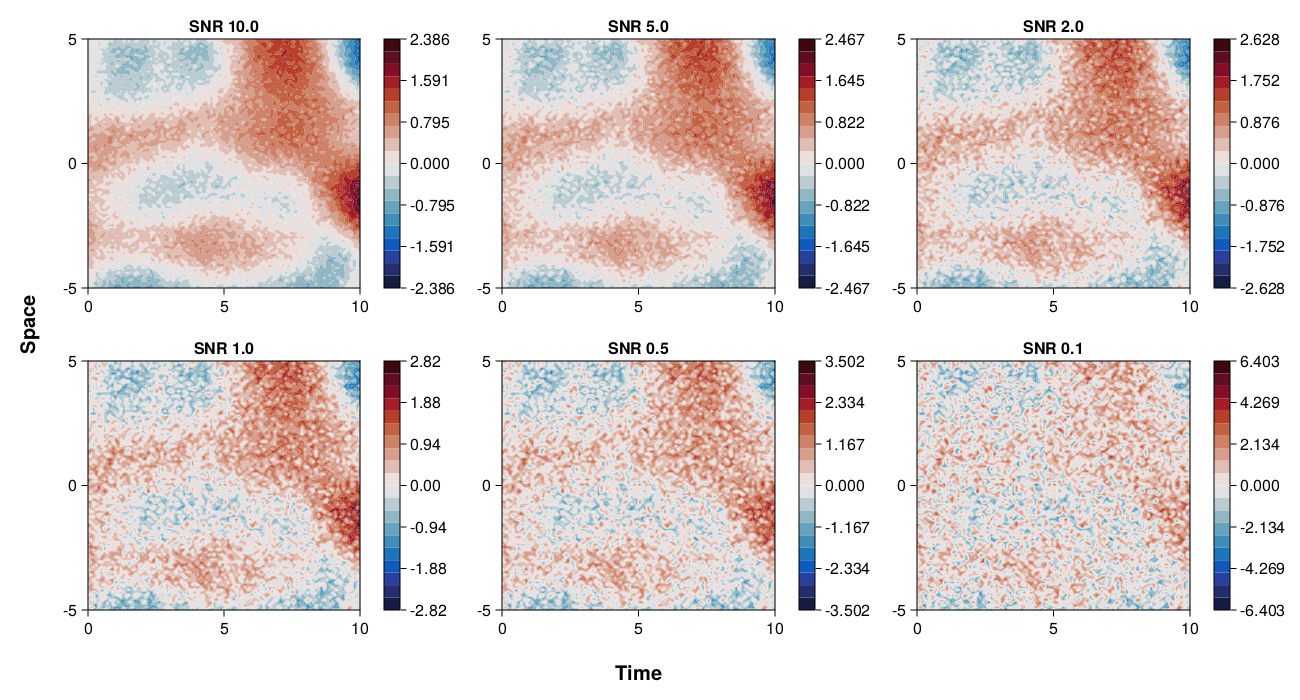
Figure S.2: Example of simulated data with varying levels of signal-to-noise ratio.

S.5 Pacific decadal oscillation

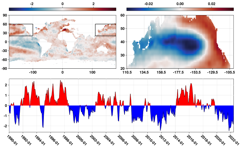
Figure S.3: Detrended monthly SST data in degrees Celsius for June 2022 (top left) where red (blue) values denote anomalously high (low) temperatures compared to historical values. The black box corresponds to the geographical region used to compute the PDO index. Note, because of the spherical nature of the data, the box “wraps” the plot. The first EOF of the PDO (top right) and the PDO time series (bottom) computed from the detrended data where red (blue) correspond to warm (cool) phases of the Pacific.

There are various approaches to computing the PDO from monthly SST data - we provide one such approach. Assume the data is organized as $SST(\mathbf{s},t)$ for $\mathbf{s}\in\mathcal{D},t\in T$.

1. Compute the mean SST for each month at each location (i.e., the average January, February, … temperature at location $\mathbf{s}$ across all years). For each location, $\overline{SST}_{J}(\mathbf{s})=E(SST(\mathbf{s},t))$ for $t\in J\subset T,J=$ January, …, December

2. Center the data by month (subtract the monthly mean), to produce a monthly anomaly data set. For each location, $SSTM(\mathbf{s},t)=SST(\mathbf{s},t)-\overline{SST}_{J}(\mathbf{s})$ for $t\in J\subset T,J=$ January, …, December

3. Subtract the global mean of SST making sure to weight each cell appropriately based on its cell size. For each location and time, $SSTC(\mathbf{s},t)=SSTM(\mathbf{s},t)-E(SSTM(\mathbf{s},t))$

4. Remove the temporal trend - For each location, regress the time-series on an intercept and time vector and then subtract the temporal trend

   1. Let $\mathbf{X}=[\bm{1},1:T]$

   2. Compute the BLUP estimate at each location as $\bm{\beta}(\mathbf{s})=\mathbf{X}(\mathbf{X}^{\prime}\mathbf{X})^{-1}\mathbf{X}^{\prime}SSTC(\mathbf{s},:)$

   3. $SSTA(\mathbf{s},:)=SSTC(\mathbf{s},:)-\mathbf{X}\bm{\beta}(\mathbf{s})$

Then $SSTA(\mathbf{s},t)$ $\mathbf{s}\in\mathcal{D},t\in T$, which is a data set containing monthly sea surface temperature anomalies, can be used to compute the PDO index.

References

- Bailey, (2012) Bailey, S. (2012). Principal component analysis with noisy and/or missing data. Publications of the Astronomical Society of the Pacific, 124(919):1015–1023.
- Berkooz, (1993) Berkooz, G. (1993). The proper orthogonal decomposition in the analysis of turbulent flows. Annual Review of Fluid Mechanics, 25(1):539–575.
- Berliner, (1996) Berliner, L. M. (1996). Hierarchical Bayesian time series models. In Maximum Entropy and Bayesian Methods, pages 15–22. Springer Netherlands, Dordrecht.
- Bezanson et al., (2017) Bezanson, J., Edelman, A., Karpinski, S., and Shah, V. B. (2017). Julia: A fresh approach to numerical computing. SIAM Review, 59(1):65–98.
- Buhmann, (2000) Buhmann, M. D. (2000). A new class of radial basis functions with compact support. Mathematics of Computation, 70(233):307–318.
- Byrne and Girolami, (2013) Byrne, S. and Girolami, M. (2013). Geodesic Monte Carlo on embedded manifolds. Scandinavian Journal of Statistics, 40(4):825–845.
- Carpenter et al., (2017) Carpenter, B., Gelman, A., Hoffman, M. D., Lee, D., Goodrich, B., Betancourt, M., Brubaker, M. A., Guo, J., Li, P., and Riddell, A. (2017). Stan: A probabilistic programming language. Journal of Statistical Software, 76(1).
- Cattell, (1966) Cattell, R. B. (1966). The scree test for the number of factors. Multivariate Behavioral Research, 1(2):245–276.
- Chen et al., (2022) Chen, Q., Cao, J., and Xia, Y. (2022). Physics-enhanced PCA for data compression in edge devices. IEEE Transactions on Green Communications and Networking, 6(3):1624–1634.
- Chikuse, (2003) Chikuse, Y. (2003). Statistics on Special Manifolds, volume 174 of Lecture Notes in Statistics. Springer New York, New York, NY.
- Cressie and Johannesson, (2006) Cressie, N. and Johannesson, G. (2006). Spatial prediction for massive datasets. Australian Academy of Science, 1247:1–11.
- Cressie and Johannesson, (2008) Cressie, N. and Johannesson, G. (2008). Fixed rank kriging for very large spatial data sets. Journal of the Royal Statistical Society: Series B (Statistical Methodology), 70(1):209–226.
- Cressie and Wikle, (2011) Cressie, N. A. C. and Wikle, C. K. (2011). Statistics For Spatio-Temporal Data. John Wiley & Sons.
- Daw et al., (2022) Daw, R., Simpson, M., Wikle, C. K., Holan, S. H., and Bradley, J. R. (2022). An overview of univariate and multivariate Karhunen Loève expansions in statistics. Journal of the Indian Society for Probability and Statistics, 23(2):285–326.
- Demmel and Kahan, (1990) Demmel, J. and Kahan, W. (1990). Accurate singular values of bidiagonal matrices. SIAM Journal on Scientific and Statistical Computing, 11(5):873–912.
- Demšar et al., (2013) Demšar, U., Harris, P., Brunsdon, C., Fotheringham, A. S., and McLoone, S. (2013). Principal component analysis on spatial data: An overview. Annals of the Association of American Geographers, 103(1):106–128.
- Epps and Krivitzky, (2019) Epps, B. P. and Krivitzky, E. M. (2019). Singular value decomposition of noisy data: noise filtering. Experiments in Fluids, 60(8):126.
- Fabrigar et al., (1999) Fabrigar, L. R., Wegener, D. T., MacCallum, R. C., and Strahan, E. J. (1999). Evaluating the use of exploratory factor analysis in psychological research. Psychological Methods, 4(3):272–299.
- Ford et al., (1986) Ford, J. K., MacCallum, R. C., and Tait, M. (1986). The application of exploratory factor analysis in applied psychology: A crictical review and analysis. Personnel Psychology, 39(2):291–314.
- Genton, (2000) Genton, M. G. (2000). Classes of kernels for machine learning: A statistics perspective. Journal of Machine Learning Research, 2:299–312.
- Gerbrands, (1981) Gerbrands, J. J. (1981). On the relationships between SVD, KLT and PCA. Pattern Recognition, 14(1-6):375–381.
- Gneiting, (2002) Gneiting, T. (2002). Compactly supported correlation functions. Journal of Multivariate Analysis, 83(2):493–508.
- Golub and Kahan, (1965) Golub, G. and Kahan, W. (1965). Calculating the singular values and pseudo-inverse of a matrix. Journal of the Society for Industrial and Applied Mathematics Series B Numerical Analysis, 2(2):205–224.
- Grotjahn et al., (2016) Grotjahn, R., Black, R., Leung, R., Wehner, M. F., Barlow, M., Bosilovich, M., Gershunov, A., Gutowski, W. J., Gyakum, J. R., Katz, R. W., Lee, Y.-Y., Lim, Y.-K., and Prabhat (2016). North American extreme temperature events and related large scale meteorological patterns: a review of statistical methods, dynamics, modeling, and trends. Climate Dynamics, 46(3-4):1151–1184.
- Hammarling, (1985) Hammarling, S. (1985). The singular value decomposition in multivariate statistics. ACM SIGNUM Newsletter, 20(3):2–25.
- Hannachi et al., (2007) Hannachi, A., Jolliffe, I. T., and Stephenson, D. B. (2007). Empirical orthogonal functions and related techniques in atmospheric science: A review. International Journal of Climatology, 27(9):1119–1152.
- Harman and Harman, (1976) Harman, H. H. and Harman, H. H. (1976). Modern factor analysis. University of Chicago Press.
- Hartmann, (2015) Hartmann, D. L. (2015). Pacific sea surface temperature and the winter of 2014. Geophysical Research Letters, 42(6):1894–1902.
- Hastie and Tibshirani, (2017) Hastie, T. and Tibshirani, R. (2017). Generalized Additive Models. Routledge.
- Heaton et al., (2019) Heaton, M. J., Datta, A., Finley, A. O., Furrer, R., Guinness, J., Guhaniyogi, R., Gerber, F., Gramacy, R. B., Hammerling, D., Katzfuss, M., Lindgren, F., Nychka, D. W., Sun, F., and Zammit-Mangion, A. (2019). A case study competition among methods for analyzing large spatial data. Journal of Agricultural, Biological and Environmental Statistics, 24(3):398–425.
- Hernandez-Stumpfhauser et al., (2017) Hernandez-Stumpfhauser, D., Breidt, F. J., and van der Woerd, M. J. (2017). The general projected normal distribution of arbitrary dimension: Modeling and Bayesian inference. Bayesian Analysis, 12(1):113–133.
- Hersbach et al., (2020) Hersbach, H., Bell, B., Berrisford, P., Hirahara, S., Horányi, A., Muñoz-Sabater, J., Nicolas, J., Peubey, C., Radu, R., Schepers, D., Simmons, A., Soci, C., Abdalla, S., Abellan, X., Balsamo, G., Bechtold, P., Biavati, G., Bidlot, J., Bonavita, M., Chiara, G., Dahlgren, P., Dee, D., Diamantakis, M., Dragani, R., Flemming, J., Forbes, R., Fuentes, M., Geer, A., Haimberger, L., Healy, S., Hogan, R. J., Hólm, E., Janisková, M., Keeley, S., Laloyaux, P., Lopez, P., Lupu, C., Radnoti, G., Rosnay, P., Rozum, I., Vamborg, F., Villaume, S., and Thépaut, J. (2020). The ERA5 global reanalysis. Quarterly Journal of the Royal Meteorological Society, 146(730):1999–2049.
- Hoff, (2007) Hoff, P. D. (2007). Model averaging and dimension selection for the singular value decomposition. Journal of the American Statistical Association, 102(478):674–685.
- Hoff, (2009) Hoff, P. D. (2009). Simulation of the matrix Bingham–von Mises–Fisher distribution, with applications to multivariate and relational data. Journal of Computational and Graphical Statistics, 18(2):438–456.
- Hotelling, (1933) Hotelling, H. (1933). Analysis of a complex of statistical variables into principal components. Journal of Educational Psychology, 24(6):417–441.
- Huang and Wand, (2013) Huang, A. and Wand, M. P. (2013). Simple marginally noninformative prior distributions for covariance matrices. Bayesian Analysis, 8(2):439–452.
- Jackson, (1993) Jackson, D. A. (1993). Stopping rules in principal components analysis: A comparison of heuristical and statistical approaches. Ecology, 74(8):2204–2214.
- Jackson and Chen, (2004) Jackson, D. A. and Chen, Y. (2004). Robust principal component analysis and outlier detection with ecological data. Environmetrics, 15(2):129–139.
- Jauch et al., (2021) Jauch, M., Hoff, P. D., and Dunson, D. B. (2021). Monte Carlo simulation on the Stiefel manifold via polar expansion. Journal of Computational and Graphical Statistics, 30(3):622–631.
- Jolliffe et al., (2002) Jolliffe, I., Uddin, M., and Vines, S. (2002). Simplified EOFs-three alternatives to rotation. Climate Research, 20(3):271–279.
- Jolliffe, (2002) Jolliffe, I. T. (2002). Principal Component Analysis. Springer Series in Statistics. Springer-Verlag, New York.
- Kambhatla and Leen, (1997) Kambhatla, N. and Leen, T. K. (1997). Dimension reduction by local principal component analysis. Neural Computation, 9(7):1493–1516.
- Karhunen, (1946) Karhunen, K. (1946). Zur spektraltheorie stochastischer prozesse. Ann. Acad. Sci. Fennicae, AI, 34.
- Loéve, (1955) Loéve, M. (1955). Probability theory: foundations, random sequences. New York, NY: Van Nostrand.
- Lorenz, (1956) Lorenz, E. N. (1956). Empirical orthogonal functions and statistical weather prediction, volume 1. Massachusetts Institute of Technology, Department of Meteorology Cambridge.
- Mantua and Hare, (2002) Mantua, N. J. and Hare, S. R. (2002). The pacific decadal oscillation.
- Mantua et al., (1997) Mantua, N. J., Hare, S. R., Zhang, Y., Wallace, J. M., and Francis, R. C. (1997). A pacific interdecadal climate oscillation with impacts on salmon production. Bulletin of the American Meteorological Society, 78(6):1069–1079.
- Mardia and Jupp, (1999) Mardia, K. V. and Jupp, P. E. (1999). Directional Statistics. Wiley Series in Probability and Statistics. John Wiley & Sons, Inc., Hoboken, NJ, USA.
- Mauldin et al., (2011) Mauldin, F. W., Lin, D., and Hossack, J. A. (2011). The singular value filter: A general filter design strategy for PCA-based signal separation in medical ultrasound imaging. IEEE Transactions on Medical Imaging, 30(11):1951–1964.
- Melkumyan and Ramos, (2009) Melkumyan, A. and Ramos, F. (2009). A sparse covariance function for exact gaussian process inference in large datasets. IJCAI International Joint Conference on Artificial Intelligence, pages 1936–1942.
- Mitchell and Beauchamp, (1988) Mitchell, T. J. and Beauchamp, J. J. (1988). Bayesian variable selection in linear regression. Journal of the American Statistical Association, 83(404):1023.
- Mulaik, (2009) Mulaik, S. A. (2009). Foundations of Factor Analysis. CRC press.
- Newman et al., (2016) Newman, M., Alexander, M. A., Ault, T. R., Cobb, K. M., Deser, C., Di Lorenzo, E., Mantua, N. J., Miller, A. J., Minobe, S., Nakamura, H., Schneider, N., Vimont, D. J., Phillips, A. S., Scott, J. D., and Smith, C. A. (2016). The pacific decadal oscillation, revisited. Journal of Climate, 29(12):4399–4427.
- Noack et al., (2023) Noack, M. M., Krishnan, H., Risser, M. D., and Reyes, K. G. (2023). Exact Gaussian processes for massive datasets via non-stationary sparsity-discovering kernels. Scientific Reports, 13(1):3155.
- North et al., (1982) North, G. R., Bell, T. L., Cahalan, R. F., and Moeng, F. J. (1982). Sampling errors in the estimation of empirical orthogonal functions. Monthly Weather Review, 110(7):699–706.
- Nychka et al., (2002) Nychka, D., Wikle, C., and Royle, J. A. (2002). Multiresolution models for nonstationary spatial covariance functions. Statistical Modelling, 2(4):315–331.
- O’Brien and Deser, (2023) O’Brien, J. P. and Deser, C. (2023). Quantifying and understanding forced changes to unforced modes of atmospheric circulation variability over the north Pacific in a coupled model large ensemble. Journal of Climate, 36(1):19–37.
- Peres-Neto et al., (2003) Peres-Neto, P. R., Jackson, D. A., and Somers, K. M. (2003). Giving meaningful interpretation to ordination axes: Assessing loading significance in principal component analysis. Ecology, 84(9):2347–2363.
- Pewsey and García-Portugués, (2021) Pewsey, A. and García-Portugués, E. (2021). Recent advances in directional statistics. TEST, 30(1):1–58.
- Pilario et al., (2019) Pilario, K. E., Shafiee, M., Cao, Y., Lao, L., and Yang, S.-H. (2019). A review of kernel methods for feature extraction in nonlinear process monitoring. Processes, 8(1):24.
- Pourzanjani et al., (2021) Pourzanjani, A. A., Jiang, R. M., Mitchell, B., Atzberger, P. J., and Petzold, L. R. (2021). Bayesian inference over the Stiefel manifold via the Givens representation. Bayesian Analysis, 16(2):639–666.
- Rayner, (2003) Rayner, N. A. (2003). Global analyses of sea surface temperature, sea ice, and night marine air temperature since the late nineteenth century. Journal of Geophysical Research, 108(D14):4407.
- Risser et al., (2021) Risser, M. D., Wehner, M. F., O’Brien, J. P., Patricola, C. M., O’Brien, T. A., Collins, W. D., Paciorek, C. J., and Huang, H. (2021). Quantifying the influence of natural climate variability on in situ measurements of seasonal total and extreme daily precipitation. Climate Dynamics, 56(9-10):3205–3230.
- Roden et al., (2015) Roden, R., Smith, T., and Sacrey, D. (2015). Geologic pattern recognition from seismic attributes: Principal component analysis and self-organizing maps. Interpretation, 3(4):SAE59–SAE83.
- Shen and Huang, (2008) Shen, H. and Huang, J. Z. (2008). Sparse principal component analysis via regularized low rank matrix approximation. Journal of Multivariate Analysis, 99(6):1015–1034.
- Smith et al., (2014) Smith, S. M., Hyvärinen, A., Varoquaux, G., Miller, K. L., and Beckmann, C. F. (2014). Group-PCA for very large fMRI datasets. NeuroImage, 101:738–749.
- Stewart, (1993) Stewart, G. W. (1993). On the early history of the singular value decomposition. SIAM Review, 35(4):551–566.
- Stroud et al., (2001) Stroud, J. R., Müller, P., and Sansö, B. (2001). Dynamic models for spatiotemporal data. Journal of the Royal Statistical Society. Series B: Statistical Methodology, 63(4):673–689.
- Thompson and Wallace, (2000) Thompson, D. W. J. and Wallace, J. M. (2000). Annular modes in the extratropical circulation. Part I: Month-to-month variability*. Journal of Climate, 13(5):1000–1016.
- Van Der Maaten et al., (2009) Van Der Maaten, L. J. P., Postma, E. O., and Van Den Herik, H. J. (2009). Dimensionality reduction: A comparative review. Journal of Machine Learning Research, 10:1–41.
- Wang and Gelfand, (2013) Wang, F. and Gelfand, A. E. (2013). Directional data analysis under the general projected normal distribution. Statistical Methodology, 10(1):113–127.
- Wang and Gelfand, (2014) Wang, F. and Gelfand, A. E. (2014). Modeling space and space-time directional data using projected Gaussian processes. Journal of the American Statistical Association, 109(508):1565–1580.
- Wang and Huang, (2017) Wang, W.-T. and Huang, H.-C. (2017). Regularized principal component analysis for spatial data. Journal of Computational and Graphical Statistics, 26(1):14–25.
- Wendland, (1995) Wendland, H. (1995). Piecewise polynomial, positive definite and compactly supported radial functions of minimal degree. Advances in Computational Mathematics, 4(1):389–396.
- Wikle, (2003) Wikle, C. K. (2003). Hierarchical Bayesian models for predicting the spread of ecological processes. Ecology, 84(6):1382–1394.
- Wikle, (2010) Wikle, C. K. (2010). Low-rank representations for spatial processes. In Gelfand, A. E., Diggle, P., Peter, G., and Montserrat, F., editors, Handbook of Spatial Statistics, chapter 8. CRC Press, Boca Raton, 1 edition.
- Wikle et al., (2019) Wikle, C. K., Zammit-Mangion, A., and Cressie, N. (2019). Spatio-Temporal Statistics with R. Chapman and Hall/CRC, Boca Raton, Florida : CRC Press, [2019].
- Wold, (1978) Wold, S. (1978). Cross-validatory estimation of the number of components in factor and principal components models. Technometrics, 20(4):397–405.
- Yu et al., (2019) Yu, C.-H., Gao, F., Lin, S., and Wang, J. (2019). Quantum data compression by principal component analysis. Quantum Information Processing, 18(8):249.
- Zhang et al., (2010) Zhang, X., Wang, J., Zwiers, F. W., and Groisman, P. Y. (2010). The influence of large-scale climate variability on winter maximum daily precipitation over North America. Journal of Climate, 23(11):2902–2915.
- Zou et al., (2006) Zou, H., Hastie, T., and Tibshirani, R. (2006). Sparse principal component analysis. Journal of Computational and Graphical Statistics, 15(2):265–286.