Revised orbits of the two nearest Jupiters

Abstract

With its near-to-mid-infrared high contrast imaging capabilities, JWST is ushering us into a golden age of directly imaging Jupiter-like planets. As the two closest cold Jupiters, $\varepsilon$ Ind A b and $\varepsilon$ Eridani b have sufficiently wide orbits and adequate infrared emissions to be detected by JWST. To detect more Jupiter-like planets for direct imaging, we develop a GOST-based method to analyze radial velocity data and multiple Gaia data releases simultaneously. Without approximating instantaneous astrometry by catalog astrometry, this approach enables the use of multiple Gaia data releases for detection of both short-period and long-period planets. We determine a mass of $2.96_{-0.38}^{+0.41}$ $M_{\rm Jup}$ and a period of $42.92_{-4.09}^{+6.38}$ yr for $\varepsilon$ Ind A b. We also find a mass of $0.76_{-0.11}^{+0.14}$ $M_{\rm Jup}$ , a period of $7.36_{-0.05}^{+0.04}$ yr, and an eccentricity of 0.26${}_{-0.04}^{+0.04}$ for $\varepsilon$ Eridani b. The eccentricity differs from that given by some previous solutions probably due to the sensitivity of orbital eccentricity to noise modeling. Our work refines the constraints on orbits and masses of the two nearest Jupiters and demonstrate the feasibility of using multiple Gaia data releases to constrain Jupiter-like planets.

1 Introduction

The detection and characterization of Jupiter-like planets in extrasolar systems are crucial for our understanding of their formation and evolution as well as their role in shaping the system architecture and habitability (Stevenson & Lunine, 1988; Lunine, 2001; Tsiganis et al., 2005; Horner et al., 2020). While the current ground-based facilities are mainly sensitive to young Jupiters, the Mid-Infrared Instrument (MIRI; Rieke et al. 2015) mounted on the James Webb Space Telescope (JWST) is optimal for imaging cold Jupiters, which are far more abundant than young Jupiters. Equipped with a coronagraph, MIRI has an imaging observing mode from 4.7 to 27.9 $\mu$m , sensitive to the mid-infrared emission from cold Jupiters with equilibrium temperature of less than 200 K (Bouchet et al., 2015). On the other hand, the JWST Near Infrared Spectrograph (NIRSpec; Jakobsen et al. 2022) conducts medium-resolution spectroscopic observation from 0.6 to 5.3 $\mu$m . The differential Doppler shift of planet relative to its host star could be used to disentangle planetary and stellar spectrums for planet imaging (Llop-Sayson et al., 2021).

Considering that high contrast imaging typically requires large planet-star separation and high planetary mass, nearby cold Jupiters are optimal targets for JWST imaging. However, the orbital periods of cold Jupiters are as long as decades, beyond most of the individual radial velocity (RV), astrometric, and transit surveys. Hence, it is important to form extremely long observational time span (or baseline) by combining different types of data. One successful application of such synergistic approach is combined analyses of legacy RV data and the astrometric data from Hipparcos (Perryman et al., 1997; van Leeuwen, 2007) and Gaia data releases (Gaia Collaboration et al., 2016; Gaia Collaboration et al., 2018, 2020; Gaia Collaboration et al., 2022). This approach not only provides decade-long baseline to constrain the orbit of a cold Jupiter but also fully constrain planetary mass and orbit due to the complementarity between RV and astrometry. Assuming that the catalog astrometry approximates the instantaneous astrometry at the reference epoch, one can use the difference between Hipparcos and Gaia astrometry to constrain the nonlinear motion of a star (or reflex motion) induced by its companion (Snellen & Brown, 2018; Brandt, 2018; Feng et al., 2019c; Kervella et al., 2019). However, under this assumption, Gaia DR2 and DR3 are not independent and thus cannot be used simultaneously to constrain planetary orbit. Moreover, this assumption is not appropriate for constraining orbits with periods comparable or shorter than the observational time span of the epoch data used to produce an astrometric catalog.

To use multiple Gaia data releases to constrain both short and long-period planets, we simulate the Gaia epoch data using the Gaia Observation Forecast Tool (GOST) and fit the synthetic data by a linear astrometric model, corresponding to the Gaia five-parameter solution. The difference between the fitted and the catalog astrometry constrains the nonlinear reflex motion induced by planets. In this work, we apply this approach to constrain the orbits and masses of the two nearest cold Jupiters, $\varepsilon$ Ind A b and $\varepsilon$ Eridani b.

This paper is structured as follows. In section 2, we introduce the RV and astrometry data measured for $\varepsilon$ Ind A and $\varepsilon$ Eridani . We then describe the modeling and statistical methods used in our analyses in section 3. We give the orbital solutions for the two planets and compare our solutions with previous ones in section 4. Finally, we discuss and conclude in section 5.

2 RV and astrometry data

$\varepsilon$ Ind A is a K-type star with a mass of 0.754$\pm$0.038 $M_{\odot}$ (Demory et al., 2009), located at a heliocentric distance of 3.7 pc. It hosts two brown dwarfs (Smith et al., 2003) and a Jupiter-like planet (Feng et al., 2019c). It has been observed by high precision spectrographs including the High Accuracy Radial Velocity Planet Searcher (HARPS; Pepe et al. 2000) mounted on the ESO La Silla 3.6m telescope, the ESO UV-visual echelle spectrograph (UVES) on Unit 2 of the Very Large Telescope (VLT) array (Dekker et al., 2000), and the Coudé Echelle Spectrograph (CES) at the 1.4 m telescope in La Silla, Chile. We use “HARPSpre” and “HARPSpost” to denote HARPS data obtained before and after the fibre change in 2015 (Lo Curto et al., 2015). The HARPS data are reduced by Trifonov et al. (2020) using the SERVAL pipeline (Zechmeister et al., 2018). The RV data obtained by the Long Camera (LC) and the Very Long Camera (VLC) were released by Zechmeister et al. (2013).

As a K-type star with a mass of 0.82$\pm$0.02 $M_{\odot}$ (Gonzalez et al., 2010), $\varepsilon$ Eridani is the third closest star system to the Earth. It is likely that a Jupiter analog orbits around this star on a wide orbit (Hatzes et al., 2000; Butler et al., 2006; Mawet et al., 2019). It has been observed by the CES LC and VLC (Zechmeister et al., 2013), the Lick Observatory Hamilton echelle spectrometer (Vogt, 1987), the Automated Planet Finder (APF; Vogt et al. 2014), the HIRES spectrometer (Vogt et al., 1994) at the Keck observatory, the HARPS for the Northern hemisphere (HARPS-N or HARPN; Cosentino et al. 2012) installed at the Italian Telescopio Nazionale Galileo (TNG), the EXtreme PREcision Spectrograph (EXPRES; Jurgenson et al. 2016) installed at the 4.3 m Lowell Discovery Telescope (LDT; Levine et al. 2012). By accounting for the RV offets caused by the updates of Lick Hamilton spectrograph, we use “Lick6”, “Lick8”, and “Lick13” to denote multiple data sets, following the convention given by Fischer et al. (2013). We use the APF and HIRES data reduced by the standard CPS pipeline (Howard et al., 2010) and released by Mawet et al. (2019) as well as the other APF data reduced using the pipeline developed by Butler et al. (1996) and the HIRES data released by Butler et al. (2017). We use “APFh” and “HIRESh” to denote the former sets and use “APFp” and “HIRESp” to denote the latter. The APFp data set is presented in Table 4. The EXPRES data is from Roettenbacher et al. (2022) and the HARPS data is obtained from Trifonov et al. (2020).

We obtain the Hipparcos epoch data for $\varepsilon$ Ind A and $\varepsilon$ Eridani from the new Hipparcos reduction (van Leeuwen, 2007). We use the Gaia second and third data releases (DR2 and DR3; Gaia Collaboration et al. 2020; Gaia Collaboration et al. 2022) as well as the epoch data generated by GOST. The Gaia first data release (DR1) is not used because it is derived partly from the Hipparcos data (Michalik et al., 2015) and is thus not treated as independent of the Hipparcos data.

3 Method

Considering that the Gaia intermediate astrometric data (or epoch data) are not available in the current Gaia data releases, techniques have been developed to use the difference between Gaia and Hipparcos catalog data to constrain the orbits of substellar companions (Brandt et al., 2019; Kervella et al., 2019; Feng et al., 2022). Without using epoch data, previous studies are limited by approximating the simultaneous astrometry at the reference epoch with the catalog astrometry (Feng et al., 2022). In other words, a linear function is not appropriate to model the center (position) and tangential line (proper motion) of the orbital arc of the stellar reflex motion induced by short-period companions.

To avoid the above assumptions, we use GOST to predict the Gaia observation epochs for a given star. Considering that the models of RV and reflex motion are already introduced in the previous papers authored by some of us (Feng et al., 2019c; Feng et al., 2021), we introduce the newly developed technique of using Hipparcos intermediate data and Gaia GOST data as follows.

• Obtain data. For a given target, we obtain the revised Hipparcos intermediate data IAD from van Leeuwen (2007) and Gaia GOST data, including the scan angle $\psi$, the along-scan (AL) parallax factor $f^{\rm AL}$, and the observation time at barycenter. In previous studies, different versions of the Hipparcos catalog data have been recommended (ESA, 1997; van Leeuwen, 2007). However, in our research, we find that the choice of the Hipparcos version has minimal impact on our orbital solutions. We attribute this to several reasons:

  • Our approach involves modeling the systematics in Hipparcos IAD using offsets and jitters instead of calibrating them a priori, as described in Brandt et al. (2023). By incorporating these offsets and jitters, we account for the systematic effects in the data, making our solutions less sensitive to the specific Hipparcos version used.

  • The astrometric precision of Hipparcos is considerably inferior to that of Gaia. Additionally, the time difference between Gaia and Hipparcos is much greater than the duration covered by Gaia data releases (DRs). Consequently, when it comes to constraining long-period orbits, the crucial factor is the temporal baseline between Hipparcos and Gaia, rather than the particular version of the Hipparcos catalog.

  • For short-period orbits, it is the curvature of the Hipparcos IAD that primarily constrains the orbit, rather than the absolute offset. Hence a calibration of the offset of Hipparcos IAD becomes less critical in determining short-period orbits.

• Model astrometry of target system barycenter (TSB) at Gaia DR3 reference epoch. We model the astrometry of the TSB at the Gaia DR3 epoch J2016.0 ($t_{\rm DR3}$) as follows:

  $$\alpha^{b}_{\rm DR3} = \alpha_{\rm DR3}-\frac{\Delta\alpha_{*}}{\cos\delta_{\rm DR3}}~{},$$ (1)

  $$\delta^{b}_{\rm DR3} = \delta_{\rm DR3}-\Delta\delta~{},$$ (2)

  $$\varpi^{b}_{\rm DR3} = \varpi_{\rm DR3}-\Delta\varpi~{},$$ (3)

  $$\mu^{b}_{\alpha{\rm DR3}} = \mu_{\alpha{\rm DR3}}-\Delta\mu_{\alpha}~{},$$ (4)

  $$\mu^{b}_{\delta{\rm DR3}} = \mu_{\delta{\rm DR3}}-\Delta\mu_{\delta}~{},$$ (5)

  where $\alpha$, $\delta$, $\varpi$, $\mu_{\alpha}$, and $\mu_{\delta}$ are R.A., decl., parallax, and proper motion in R.A and decl., subscript _DR3 represents quantities at epoch $t_{\rm DR3}$, superscript ^b represents TSB, and $\Delta$ means offset. Considering that the Gaia measurements of systematic RVs are quite uncertain, we use Gaia DR3 RVs to propagate astrometry instead of using them to constrain reflex motion.

• Model astrometry of TSB at Hipparcos and Gaia DR3 reference epochs. We model the TSB astrometry at the Hipparcos reference epoch $t_{\rm HIP}$ through linear propagation of state vectors in the Cartesian coordinate system as follows:

  $$\vec{r}_{\rm HIP}^{b} = \vec{r}^{b}_{\rm DR3}+\vec{v}^{b}_{\rm DR3}(t_{\rm HIP}-t_{\rm DR3})~{},$$ (6)

  $$\vec{v}_{\rm HIP}^{b} = \vec{v}^{b}_{\rm DR3}~{},$$ (7)

  where $(\vec{r}_{\rm HIP}^{b},\vec{v}_{\rm HIP}^{b})$ and $(\vec{r}_{\rm DR3}^{b},\vec{v}_{\rm DR3}^{b})$ are respectively the state vectors, including location and velocity, of the TSB at the Hipparcos and Gaia DR3 epochs. We first transform TSB astrometry from equatorial coordinate system, $\vec{\iota}^{b}_{\rm DR3}=(\alpha^{b}_{\rm DR3},\delta^{b}_{\rm DR3},\varpi^{b}_{\rm DR3},\mu^{b}_{\alpha{\rm DR3}},\mu^{b}_{\delta{\rm DR3}},{\rm RV}_{\rm DR3})$, to Cartesian coordinate system to get state vector at Gaia DR3 epoch, and then propagate the vector to the Hipparcos epoch, and then transform the new vector back to the astrometry at the Hipparcos epoch, $\vec{\iota}^{b}_{\rm HIP}$. The whole process is: equatorial state vector at $t_{\rm DR3}$ $\rightarrow$ Cartesian state vector at $t_{\rm DR3}$ $\rightarrow$ linear propagation of Cartesian state vector to $t_{\rm HIP}$ $\rightarrow$ equatorial state vector at $t_{\rm HIP}$. By propagating state vectors in Cartesian coordinate system instead of spherical coordinate system, this approach completely solve the problem of perspective acceleration. The transformation between different coordinate systems is described in Lindegren et al. (2012) and Feng et al. (2019b).

• Simulate Gaia abscissae using GOST. Instead of simulating the Gaia epoch data precisely by considering relativistic effects, perspective acceleration, and instrumental effects (Lindegren et al., 2012), we simulate the Gaia abscissae (or along-scan coordinates) by only considering linear motion of the TSB in the equatorial coordinate system as well as the target reflex motion . This is justified because the various effects are independent of reflex motion, and can be estimated and subtracted from the data a priori.

  We simulate the position of the target at GOST epoch $t_{j}$ relative to the Gaia DR3 reference position by adding the stellar reflex motion (denoted by superscript ^r) onto the TSB motion,

  $$\Delta\alpha_{*i} = \Delta\alpha^{b}_{*\rm DR3}+\mu_{\alpha{\rm DR3}}^{b}(t_{i}-t_{\rm DR3})+\Delta\alpha^{r}_{*i}~{},$$ (8)

  $$\Delta\delta_{i} = \Delta\delta^{b}_{\rm DR3}+\mu_{\delta{\rm DR3}}^{b}(t_{i}-t_{\rm DR3})+\Delta\delta^{r}_{i}~{},$$ (9)

  where $\Delta\alpha^{b}_{*\rm DR3}=(\alpha^{b}_{\rm DR3}-\alpha_{\rm DR3})\cos\delta^{b}_{\rm DR3}$, and $\Delta\delta^{b}_{\rm DR3}=\delta^{b}_{\rm DR3}-\delta_{\rm DR3}$. Because the reflex motion caused by cold Jupiters is insignificant compared with barycentric motion, the parallax at epoch $t_{i}$ is approximately $\varpi_{i}=\varpi^{b}_{i}+\Delta\varpi^{r}_{i}=\varpi^{b}_{\rm DR3}+\Delta\varpi^{r}_{i}\approx\varpi^{b}_{\rm DR3}$, and the systematic radial velocity is approximately ${\rm RV}_{i}={\rm RV}^{b}_{i}+\Delta{\rm RV}^{r}={\rm RV}^{b}_{\rm DR3}+\Delta{\rm RV}^{r}\approx{\rm RV}_{\rm DR3}$.

  Considering that Gaia pixels in along-scan (AL) direction are much smaller than that in the cross-scan direction, we only model the along-scan position of the target (or abscissa; $\eta_{i}$). Considering the parallax caused by Gaia’s heliocentric motion, abscissa is modeled by projecting the motion of the target onto the AL direction using

  $$\eta_{i}=\Delta\alpha_{*i}\sin\psi_{i}+\Delta\delta_{i}\cos\psi_{i}+\varpi^{b}_{\rm DR3}f^{\rm AL}_{i}~{}.$$ (10)

• Fit a five-parameter model to synthetic Gaia abscissae. Considering that binary solution is only applied to a small fraction of DR3 targets and most planet-induced reflex motion is not yet available in the Gaia non-single star catalog (Gaia Collaboration et al., 2022), we model the simulated abscissae using a five-parameter model as follows:

  $$\hat{\eta}_{i} = \Delta\alpha_{*{\rm DR3}}^{l}\sin\psi_{i}+\Delta\delta_{\rm DR3}^{l}\cos\psi_{i}+\hat{\varpi}_{\rm DR3}f^{\rm AL}_{i}~{},$$ (11)

  $$\Delta\alpha_{*{\rm DR3}}^{l} = (\hat{\alpha}_{\rm DR3}-\alpha_{\rm DR3})\cos\hat{\delta}_{\rm DR3}+\hat{\mu}_{\alpha{\rm DR3}}(t_{i}-t_{\rm DR3})~{},$$ (12)

  $$\Delta\delta_{\rm DR3}^{l} = (\hat{\delta}_{\rm DR3}-\delta_{\rm DR3})+\hat{\mu}_{\delta{\rm DR3}}(t_{i}-t_{\rm DR3})~{},$$ (13)

  where $\hat{\vec{\iota}}_{\rm DR3}=(\hat{\alpha}_{\rm DR3},\hat{\delta}_{\rm DR3},\hat{\varpi}_{\rm DR3},\hat{\mu}_{\alpha{\rm DR3}},\hat{\mu}_{\delta{\rm DR3}})$ is the set of model parameters at $t_{\rm DR3}$, $f_{i}^{\rm AL}$ is the along-scan parallax factor, and $\psi_{i}$ is the scan angle at epoch $t_{i}$. This scan angle is the complementary angle of $\psi$ in the new Hipparcos IAD (van Leeuwen, 2007; Brandt et al., 2021b; Holl et al., 2022), and thus $\psi$ will be replaced by $\pi/2-\psi$ when modeling Hipparcos IAD. The above modeling of Gaia DR3 can be applied to Gaia DR2 by changing the subscript _DR3 into _DR2. Given the limited information available through GOST, we are unable to reconstruct the uncertainties of individual observations and which epochs are actually used in producing the catalogs. As long as the astrometric uncertainties and rejected epochs are not significantly time-dependent, it is reasonable to assume that all GOST epochs are used in the astrometric solution of Gaia and all abscissae have the same uncertainty. Under this assumption, we fit the five-parameter model shown in eq. 11 to the simulated abscissae ($\eta_{i}$) for Gaia DR2 and DR3 through linear regression.

• Calculate the likelihood for Gaia DR2 and DR3. To avoid numerical errors, the catalog astrometry at $t_{i}$ relative to the Gaia DR3 epoch is defined as $\Delta\vec{\iota}_{i}\equiv(\Delta\alpha_{*i},\Delta\delta_{i},\Delta\varpi_{i},\Delta\mu_{\alpha i},\Delta\mu_{\delta i})=((\alpha_{i}-\alpha_{\rm DR3})\cos\delta_{i},\delta_{i}-\delta_{\rm DR3},\varpi_{i}-\varpi_{\rm DR3},\mu_{\alpha i}-\mu_{\alpha{\rm DR3}},\mu_{\delta i}-\mu_{\delta{\rm DR3}})$. The fitted astrometry for epoch $t_{i}$ is $\Delta\hat{\vec{\iota}}_{i}$. The likelihood for Gaia DR2 and DR3 is

  $$\mathcal{L}_{\rm gaia}=\prod_{i=1}^{N_{\rm DR}}(2\pi)^{-5/2}({\rm det}\Sigma^{\prime}_{i})^{-\frac{1}{2}}e^{-\frac{1}{2}(\Delta\hat{\vec{\iota}}_{i}-\Delta\vec{\iota}_{i})^{T}[\Sigma_{i}(1+J_{i})]^{-1}(\Delta\hat{\vec{\iota}}_{i}-\Delta\vec{\iota}_{i})}~{},$$ (14)

  where $N_{\rm DR}$ is the number of data releases used in the analyses, and $\Sigma_{i}(1+J_{i})$ is the jitter-corrected covariance for the five-parameter solutions of Gaia DRs, $i=1$ and 2 respresent Gaia DR2 and DR3, respectively. In this work, we only use DR2 and DR3 and thus $N_{\rm DR}=2$.

• Calculate the likelihood for Hipparcos intermediate data. We model the abscissae of Hipparcos ($\xi$) by adding the reflex motion onto the linear model shown in eq. 11, and calculate the likelihood as follows:

  $$\mathcal{L}_{\rm hip}=\prod\limits_{i=1}^{N_{\rm epoch}}\frac{1}{\sqrt{2\pi(\sigma_{i}^{2}+J_{\rm hip}^{2})}}e^{-\frac{(\hat{\xi}_{i}-\xi_{i})^{2}}{2(\sigma_{i}^{2}+J_{\rm hip}^{2})}},$$ (15)

  where $N_{\rm epoch}$ is the total number of epochs of Hipparcos IAD.

To obtain the total likelihood ($\mathcal{L}=\mathcal{L}_{\rm RV}\cdot\mathcal{L}_{\rm hip}\cdot\mathcal{L}_{\rm gaia}$), we derive the likelihoods for the Gaia and Hipparcos data through the above steps, and calculate the likelihood for the RV data ($\mathcal{L}_{\rm RV}$) following Feng et al. (2017). We adopt log uniform priors for time-scale parameters such as period and correlation time scale in the moving average (MA) model (Feng et al., 2017) and uniform priors for other parameters. Finally, we infer the orbital parameters by sampling the posterior through adaptive and parallel Markov Chain Monte Carlo (MCMC) developed by Haario et al. (2001) and Feng et al. (2019a).

While packages like orbitize (Blunt et al., 2020), FORECAST (Bonavita et al., 2022), BINARYS (Leclerc et al., 2023), and kepmodel (Delisle & Ségransan, 2022) have been developed to analyze imaging, RV, and astrometric data, they are not primarily designed for analyzing Gaia catalog data as performed by orvara (Brandt et al., 2021a) and htof (Brandt et al., 2021b). Compared with orvara and htof, our method has the following features:

• we simultaneously optimize all model parameters through MCMC posterior sampling;

• we utilize multiple Gaia data releases by fitting multiple five-parameter models to Gaia epoch data simulated by GOST;

• instead of conducting calibration a priori, we employ jitters and offsets to model systematics a posteriori;

• we model time-correlated noise in the RV data.

While the use of multiple Gaia DRs does not significantly improve the constraint on long-period orbits by increasing the temporal baseline between Gaia and Hipparcos, it does provide additional information about the raw abscissae. This, in turn, leads to stronger orbital constraints at Gaia epochs. In other words, Gaia DR2 provides a 5D astrometric data point, and when combined with the 5D data point from Gaia DR3, the orbital constraint becomes stronger. The additional information obtained from multiple DRs enhances the accuracy and reliability of our orbital solutions.

Through sensitivity tests, we find that our orbital solutions are not strongly sensitive to whether or not we calibrate frame rotation and zero-point parallax a priori by adopting values from previous studies (Brandt, 2018; Kervella et al., 2019; Lindegren, 2020). It is important to note that there is uncertainty in the estimation of these calibration parameters, as indicated by studies such as Brandt (2018) and Lindegren (2020). Additionally, uncertainties can be amplified during the transformation from the Gaia frame to the Hipparcos frame. Considering these factors, it is more appropriate to consider astrometric systematics on a case-by-case basis, taking into account individual target characteristics. These issues have been discussed in our previous work (Feng et al., 2021).

To validate the accuracy of GOST emulations, we perform a comparison between the astrometric epochs generated by GOST and the G band transit times provided in Gaia Data Release 3 (GDR3) for a randomly selected sample of 1000 stars that have epoch photometry. We assess the number of mismatched epochs between GOST and the GDR3 epoch-photometry catalog, as well as the distribution of these mismatches. We define $N_{\rm gp}$ as the number of epochs predicted by GOST but not present in the GDR3 epoch-photometry catalog, and $N_{\rm pg}$ as the number of epochs present in the photometry catalog but not predicted by GOST. The distribution of the sample over G magnitude and the number of mismatched epochs is depicted in Figure 1. Notably, it is apparent that for bright stars with G magnitudes less than 10, the number of photometric epochs mismatched between GOST and GDR3 is at most 1.

To quantify the fraction of missing epochs relative to the total photometric epochs, we calculate $\eta_{\rm gp}=N_{\rm gp}/N_{p}$ and $\eta_{\rm pg}=N_{\rm pg}/N_{p}$, where $N_{p}$ represents the total number of G band photometric transits. The median of $N_{p}$ is 22. The mean values of $\eta_{\rm gp}$ and $\eta_{\rm pg}$ for bright stars are found to be 2.1% and 0.7%, respectively. For all stars, the mean values of $\eta_{\rm gp}$ and $\eta_{\rm pg}$ are 7.0% and 0.9%, respectively. This analysis serves as a validation of the accuracy of GOST emulations, further supporting the reliability of our approach.

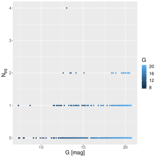
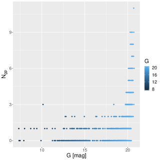
Figure 1: Distribution of 1000 stars over the G-band magnitude and the number of mismatched epochs between GOST and the GDR3 epoch-photometry catalog. The left panel is for $N_{\rm pg}$ while the right panel is for $N_{\rm gp}$.

4 Results

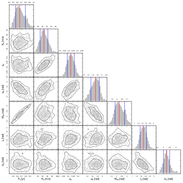
Figure 4: Corner plot showing the 1D and 2D posterior distribution of the orbital parameters for $\varepsilon$ Ind A b. In each histogram, the blue lines indicate the 1$\sigma$ confidence intervals, while the red line represents the median of the posterior distribution. The contour lines depict the 1$\sigma$ and 2$\sigma$ confidence intervals. Grey dots represent the posterior samples for each pair of parameters. It is important to note that $\omega_{b}$ denotes the argument of periastron for the stellar reflex motion, while the argument of periastron for the planetary orbit, $\omega_{p}$, is equal to $\omega_{b}+\pi$. Furthermore, $M_{0b}$ corresponds to the mean anomaly at JD 2447047.96844.

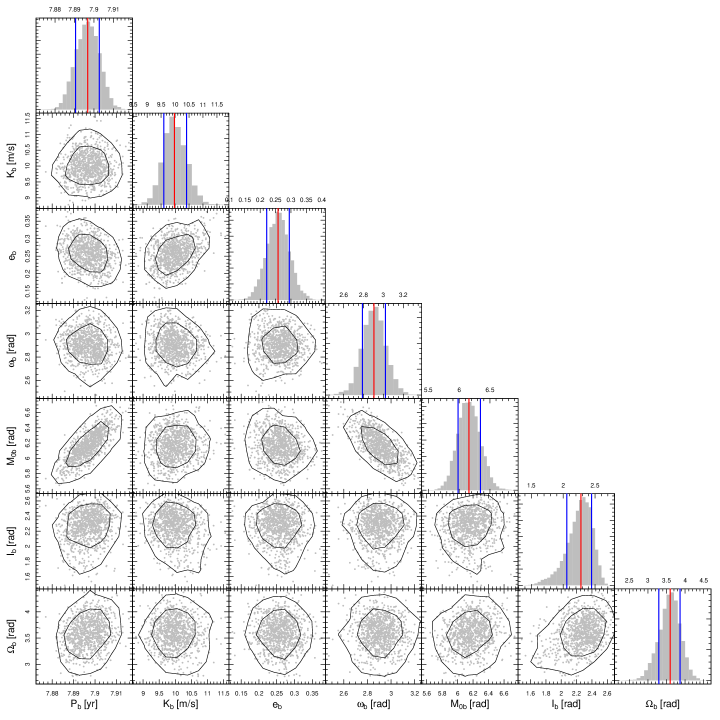
Figure 5: Similar to Fig. 4, but for $\varepsilon$ Eridani b. $M_{0b}$ is the mean anomaly at JD 2448930.56223.

We find the optimal orbital solutions for $\varepsilon$ Ind A b and $\varepsilon$ Eridani b based on the MCMC samplings of posteriors and show the solutions in Fig. 2 and the posterior distributions of orbital parameters in Fig. 4 and Fig. 5. To optimize the visualization of Fig. 2, we project the synthetic abscissae along the R.A. and decl. direction, encode the orbital phase with colors, and represent the orbital direction using circles with arrows. In the panels for Gaia synthetic abscissae (third column), we use segments and shaded regions to visualize the catalog astrometry ($\Delta\vec{\iota}-\Delta\hat{\vec{\iota}}^{b}$) and fitted astrometry ($\Delta\hat{\vec{\iota}}-\Delta\hat{\vec{\iota}}^{b}$) after subtracting the astrometry of TSB, respectively. The center of the segment is determined by the R.A. and decl. relative to the TSB, the slope is the ratio of proper motion offsets in the decl. and R.A directions, and the length is equal to the proper motion offset multiplied by the time span of Gaia DR2 or DR3. The fitted astrometry is determined through a five-parameter linear fit to the synthetic data, which is represented by colorful dots in the panels of the third column of Fig. 2. We also predict the position of $\varepsilon$ Ind A b and $\varepsilon$ Eridani b on January 1st, 2024. Their angular separations are 2.1$\pm$0.1^′′and 0.64$\pm$0.10^′′, and position angles are $243\pm 14$^∘and $258\pm 30$^∘, respectively. In addition, we present the fit to the five-parameter astrometry of Gaia DR2 and DR3 in Fig. 3. It is apparent that the deviation caused by $\varepsilon$ Ind A b from the barycentric astrometry is more pronounced compared to that induced by $\varepsilon$ Eridani b. The model fit consistently remains within 1-$\sigma$ of the five-parameter catalog astrometry.

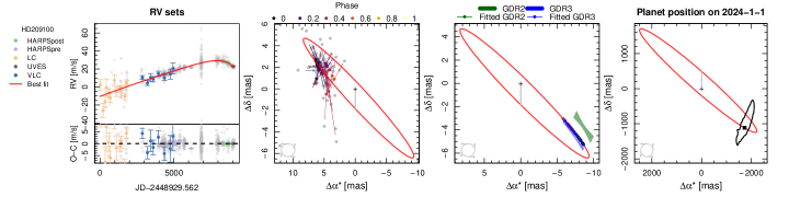
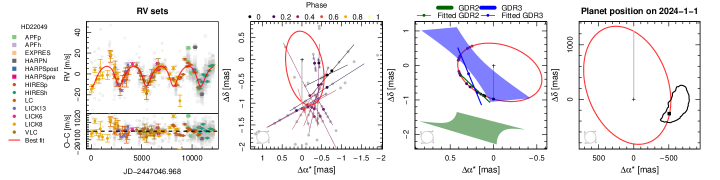
Figure 2: Optimal orbital solutions for $\varepsilon$ Ind A b (top) and $\varepsilon$ Eridani b (bottom). The panels from the left to the right respectively show the best fit to RV, Hipparcos IAD, and Gaia GOST data, and the predicted planetary position on January 1st, 2024. The first column shows the binned RV data sets encoded by colors and shapes. For optimal visualization, each RV set is binned with a 100 d time window while the un-binned RVs and residuals are shown in grey. The second column shows the post-fit Hipparcos abscissa residual projected along the R.A. and decl. directions. The multiple measurements for each epoch are binned to present the binned data encoded by colors. The darker colors encode earlier phases while the brighter colors represent later phases. The directions of the error bars indicate the along-scan direction. The third column shows the optimal fit to the Gaia GOST data and the comparison between best-fit and catalog proper motions and positions at Gaia DR2 (GDR2) and GDR3 reference epochs. The shaded regions represent the uncertainty of position and proper motion. The dot and slope of each line respectively represent the best-fit position and proper motion offsets induced by the reflex motion at certain reference epoch. The fourth column shows the predicted planet position on January 1st, 2024. The 1-$\sigma$ contour line is shown to indicate the prediction uncertainty.

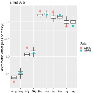
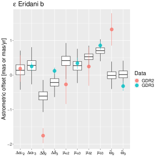
Figure 3: Model fit to the five-parameter astrometry of GDR2 and GDR3 for $\varepsilon$ Ind A b (left) and $\varepsilon$ Eridani b (right). In both cases, the barycentric astrometry is subtracted from the five-parameter solutions for both the data (represented by a dot with error bar) and the model prediction (represented by a boxplot). The subscripts of the labels on the x-axes indicate the Gaia data release number.

The inferred parameters are presented in Table 1, 2, and 3. In the table, the following orbital parameters are directly inferred through posterior sampling: the orbital period ($P$), RV semi-amplitude ($K$), eccentricity ($e$), argument of periastron ($\omega$) of the stellar reflex motion, inclination ($I$), longitude of ascending node ($\Omega$), and mean anomaly at the minimum epoch of RV data ($M_{0}$). The table also presents the astrometric offsets, which need to be subtracted from the catalog astrometry of Gaia DR3 to derive the TSB astrometry. The bottom three rows present the derived parameters, including the semi-major axis of the planet-star binary orbit ($a$), planet mass ($m_{p}$), and the epoch when a planet crosses through its periastron ($T_{p}$).

Table 1: Parameters for $\varepsilon$ Ind A b and $\varepsilon$ Eridani b.

Parametera	Unit	Meaning	$\varepsilon$ Ind A b	$\varepsilon$ Eridani b	Priorc	Minimum	Maximum
$P$	day	Orbital period	$15676.48_{-1492.59}^{+2331.54}$	$2688.60_{-16.51}^{+16.17}$	Log-Uniform	-1	16
$K$	m s-1	RV semi-amplitude	$31.69_{-4.25}^{+4.55}$	$9.98_{-0.38}^{+0.43}$	Uniform	$10^{-6}$	$10^{6}$
$e$	—	Eccentricity	$0.42_{-0.04}^{+0.04}$	$0.26_{-0.04}^{+0.04}$	Uniform	0	1
$\omega$b	deg	Argument of periapsis	$98.73_{-11.46}^{+9.46}$	$166.48_{-6.66}^{+6.63}$	Uniform	0	2$\pi$
$I$	deg	Inclination	$84.41_{-9.94}^{+9.36}$	$130.60_{-12.62}^{+9.53}$	CosI-Uniform	-1	1
$\Omega$	deg	Longitude of ascending node	$243.38_{-13.41}^{+14.36}$	$206.07_{-17.48}^{+15.14}$	Uniform	0	2$\pi$
$M_{0}$	deg	Mean anomaly at the reference epoch	$127.64_{-24.09}^{+31.05}$	$352.80_{-10.00}^{+10.80}$	Uniform	0	2$\pi$
$\Delta\alpha$	mas	$\alpha$ offset	$-7.51_{-1.72}^{+1.59}$	$0.26_{-0.20}^{+0.19}$	Uniform	$-10^{6}$	$10^{6}$
$\Delta\delta$	mas	$\delta$ offset	$-3.83_{-2.16}^{+2.40}$	$-0.04_{-0.20}^{+0.18}$	Uniform	$-10^{6}$	$10^{6}$
$\Delta\varpi$	mas	$\varpi$ offset	$-0.59_{-0.33}^{+0.28}$	$-0.31_{-0.15}^{+0.14}$	Uniform	$-10^{6}$	$10^{6}$
$\Delta\mu^{*}_{\alpha}$	mas yr-1	$\mu^{*}_{\alpha}$ offset	$1.00_{-0.08}^{+0.11}$	$0.36_{-0.02}^{+0.02}$	Uniform	$-10^{6}$	$10^{6}$
$\Delta\mu_{\delta}$	mas yr-1	$\mu_{\delta}$ offset	$0.95_{-0.19}^{+0.21}$	$0.85_{-0.01}^{+0.01}$	Uniform	$-10^{6}$	$10^{6}$
$P$	yr	Orbital period	$42.92_{-4.09}^{+6.38}$	$7.36_{-0.05}^{+0.04}$	—	—	—
$a$	au	Semi-major axis	$11.08_{-0.74}^{+1.07}$	$3.53_{-0.06}^{+0.06}$	—	—	—
$m_{p}$	$M_{\rm Jup}$	Planet mass	$2.96_{-0.38}^{+0.41}$	$0.76_{-0.11}^{+0.14}$	—	—	—
$T_{p}-2400000$	JD	Periapsis epoch	$43293.68_{-1455.27}^{+1202.96}$	$44411.54_{-81.95}^{+76.60}$	—	—	—
a The first 12 rows show parameters that are inferred directly through MCMC posterior sampling, while the last five rows show the parameters derived from the directly sampled parameters. The semi-major axis $a$ and planet mass $m_{p}$ are derived from the orbital parameters by adopting a stellar mass of 0.81$\pm$0.04 $M_{\odot}$ for $\varepsilon$ Eridani and 0.74$\pm$0.04 $M_{\odot}$ for $\varepsilon$ Ind A from the Gaia Final Luminosity Age Mass Estimator (Creevey et al., 2022).
b This is the argument of periastron of stellar reflex motion and $\omega+\pi$ is the argument of periastron of planetary orbit.
c The rightest three columns show the prior distribution and the corresponding minimum and maximum values for a parameter. “Log-Uniform” is the logarithmic uniform distribution, and “CosI-Uniform” is the uniform distribution over $\cos I$.

As the nearest cold Jupiters, $\varepsilon$ Ind A b and $\varepsilon$ Eridani b have been intensively studied in the past. Here we compare our solutions with previous ones. Based on combined analyses of RV, Hipparcos and Gaia DR2, Feng et al. (2019c) determine a mass of 3.25${}_{-0.65}^{+0.39}$ $M_{\rm Jup}$ , a period of $45.20^{+5.74}_{-4.77}$ yr, and an eccentricity of $0.26_{-0.03}^{+0.07}$ for $\varepsilon$ Ind A b. Recently, Philipot et al. (2023) analyze the RV, Hipparcos and Gaia early data release 3 (EDR3; Gaia Collaboration et al. 2022) data using the HTOF package (Brandt et al., 2021b), and estimate a mass of $3.0\pm 0.1$ $M_{\rm Jup}$ , a period of $29.93_{-0.62}^{+0.73}$ yr, and an eccentricity of $0.48\pm 0.01$. In addition to the Gaia EDR3 (equivalent to DR3 for five-parameter solutions) data used by Philipot et al. (2023), we use Gaia DR2 to constrain the orbit. We find a mass of $2.96_{-0.38}^{+0.41}$ $M_{\rm Jup}$ , a period of $42.92^{+6.38}_{-4.09}$ yr, and an eccentricity of $0.42_{-0.04}^{+0.04}$. The orbital period estimated in this work and in Feng et al. (2019c) is significantly longer than the one given by Philipot et al. (2023) probably due to the following reasons: (1) we optimize all parameters simultaneously instead of marginalizing some of them; (2) as suggested by Zechmeister et al. (2013), we subtract the perspective acceleration (about 1.8 m s^-1yr^-1) from both the CES LC and VLC sets; (3) we model the time-correlated RV noise as well as instrument-dependent jitters (Feng et al., 2019c); (4) we use astrometric data from both Gaia DR2 and DR3. A detailed comparison of our methodology with others is given by Feng et al. (2021).

Although the existence of a cold Jupiter around $\varepsilon$ Eridani was disputed due to consideration of stellar activity cycles in RV analyses (Hatzes et al., 2000; Anglada-Escudé & Butler, 2012), $\varepsilon$ Eridani b has been gradually confirmed by combined analyses of RV, astrometry, and imaging data (Benedict et al., 2017; Mawet et al., 2019; Llop-Sayson et al., 2021; Benedict, 2022; Roettenbacher et al., 2022). Based on RV constraint and direct imaging upper limit of $\varepsilon$ Eridani b, Mawet et al. (2019) determine a mass of $0.78_{-0.12}^{+0.38}$ $M_{\rm Jup}$ , a period of $7.37\pm 0.07$ yr, and an eccentricity of $0.07_{-0.05}^{+0.06}$. Llop-Sayson et al. (2021) analyze RV, absolute astrometry from Hipparcos and Gaia DR2, and imaging data, and estimate a mass of $0.66_{-0.09}^{+0.12}$ $M_{\rm Jup}$ , a period of $2671_{-23}^{+17}$ d, and an eccentricity of $0.055_{-0.039}^{+0.067}$. With additional RV data from EXPRES, Roettenbacher et al. (2022) get a solution consistent with that given by Mawet et al. (2019). Using only the astrometric data obtained by the Fine Guidance Sensor 1r of HST, Benedict (2022) determines a mass of $0.63_{-0.04}^{+0.12}$ $M_{\rm Jup}$ , a period of 2775$\pm$5 d, and an eccentricity of 0.16$\pm$0.01. In this work, the combined analyses of RV, Hipparcos, Gaia DR2 and DR3 astrometry determine a mass of $0.76_{-0.11}^{+0.14}$ $M_{\rm Jup}$ , a period of $2688.60_{-16.51}^{+16.17}$ d, and an eccentricity of 0.26$\pm$0.04. Modeling the time-correlated RV noise using the MA model, our solution gives an eccentricity significantly higher than the value given by Mawet et al. (2019), Llop-Sayson et al. (2021), and Roettenbacher et al. (2022), who use Gaussian processes to model time-correlated RV noise. While Gaussian process interprets the extra RV variations at the peaks and troughs of the Keplerian signal as time-correlated noise (see the bottom left panel of Fig. 2 in this paper and fig. 2 in Roettenbacher et al. 2022), we interpret them as part of the signal because these excessive variations always amplify the peaks and troughs at the corresponding epochs with a similar periodicity. In previous studies where Gaussian process is not employed in RV modeling, high eccentricities have typically been estimated, such as $0.608\pm 0.041$(Hatzes et al., 2000), $0.25\pm 0.23$ (Butler et al., 2006), and $0.40\pm 0.11$(Anglada-Escudé & Butler, 2012). Furthermore, astrometry-only analyses have also resulted in high-eccentricity solutions, as demonstrated by previous studies such as $e=0.702\pm 0.039$ (Benedict et al., 2006) and $e=0.16\pm 0.01$ (Benedict, 2022). Therefore, it is plausible to conclude that the orbital eccentricity of $\varepsilon$ Eridani b is significantly higher than zero, as indicated by the findings of this study. In our study, the inclination is $130.60_{-12.62}^{+9.53}$^∘. This is equivalent to an inclination of $49.40_{-9.53}^{+12.62}$^∘, which is calculated in the absence of knowledge regarding the longitude of the ascending node. This value is largely consistent with the debris disk inclination ranging from 17^∘to 34^∘(MacGregor et al., 2015; Booth et al., 2017) while Llop-Sayson et al. (2021) determines a significantly high inclination of $78.81_{-22.41}^{+29.34}$^∘.

5 Conclusion

Using GOST to emulate Gaia epoch data, we analyze both Gaia DR2 and DR3 data in combination with Hipparcos and RV data to constrain the orbits of the nearest Jupiters. For $\varepsilon$ Ind A b and $\varepsilon$ Eridani b, the orbital periods are $42.92_{-4.09}^{+6.38}$ yr and $7.36_{-0.05}^{+0.04}$ yr, the eccentricities are $0.42_{-0.04}^{+0.04}$ and $0.26_{-0.04}^{+0.04}$, and the masses are $2.96_{-0.38}^{+0.41}$ $M_{\rm Jup}$ and $0.76_{-0.11}^{+0.14}$ $M_{\rm Jup}$ , respectively. It is the first time that both Gaia DR2 and DR3 catalog data are modeled and analyzed by emulating the Gaia epoch data with GOST. Compared with previous studies, our approach avoids approximating instantaneous astrometry by catalog astrometry at the reference epoch, and thus enable robust constraint of orbits with period comparable or shorter than the DR2 and DR3 observation time span.

The orbital period of $\varepsilon$ Ind A b in this work is much longer than the value given by Philipot et al. (2023), but is consistent with the solution based on combined analyses of RV and Gaia DR2 (Feng et al., 2019c). While we estimate an orbital eccentricity of $\varepsilon$ Eridani b much higher than value given by Mawet et al. (2019), Llop-Sayson et al. (2021) and Roettenbacher et al. (2022) who use Gaussian process to model time-correlated noise, our solution is largely consistent with previous studies (Hatzes et al., 2000; Anglada-Escudé & Butler, 2012; Benedict et al., 2006; Benedict, 2022), which don’t use Gaussian process to model stellar activity. It is possible that Gaussian process may interpret part of the Keplerian signal as time-correlated noise (Feng et al., 2016; Ribas et al., 2018).

The combined RV and astrometry model presented in this work shares similarities with the successful model used to detect and confirm numerous sub-stellar and planetary companions in previous studies (Feng et al., 2019c; Feng et al., 2021, 2022). The orbital solution obtained for $\varepsilon$ Ind A using our new method aligns closely with the results determined in Feng et al. (2019c), which highlights the reliability of our approach in detecting cold and massive companions. The upcoming imaging observations of $\varepsilon$ Eridani and $\varepsilon$ Ind A with JWST will provide further validation of our method, particularly in utilizing multiple Gaia DRs to identify cold Jupiters. While future Gaia DR4 will release epoch data, the modeling framework developed in our study offers a general methodology for incorporating both catalog data and epoch data to constrain orbital parameters. This approach can be extended to combined analyses of astrometric data from various sources, including Gaia, photographic plates (Cerny et al., 2021), Tycho-2 (Høg et al., 2000), and future space missions such as the China Space Station Telescope (Fu et al., 2023) and the Nancy Roman Space Telescope (Yahalomi et al., 2021).

Data Availability

The new RV data are available in the appendix while the Gaia and Hipaprcos data are publicly available.

Appendix A Posterior distribution of orbital parameters

Appendix B Other model parameters

Table 2: Other parameters for $\varepsilon$ Ind A b.

Parametera	Unit	Meaning	$\varepsilon$ Ind A b	Prior	Minimum	Maximum
$\gamma^{\rm HARPSpost}$	m s-1	RV offset for HARPSpost	$-28.17_{-3.31}^{+2.97}$	Uniform	$-10^{6}$	$10^{6}$
$J^{\rm HARPSpost}$	m s-1	RV jitter for HARPSpost	$1.11_{-0.08}^{+0.09}$	Uniform	0	$10^{6}$
$w_{1}^{\rm HARPSpost}$	—	Amplitude of component 1 of MA(1) for HARPSpost	$0.97_{-0.02}^{+0.02}$	Uniform	-1	1
ln$\tau^{\rm HARPSpost}$	—	Logarithmic time scale of MA(1) for HARPSpost	$1.01_{-0.21}^{+0.21}$	Uniform	-12	12
$\gamma^{\rm HARPSpre}$	m s-1	RV offset for HARPSpre	$-25.62_{-3.33}^{+3.01}$	Uniform	$-10^{6}$	$10^{6}$
$J^{\rm HARPSpre}$	m s-1	RV jitter for HARPSpre	$1.00_{-0.01}^{+0.01}$	Uniform	0	$10^{6}$
$w_{1}^{\rm HARPSpre}$	—	Amplitude of component 1 of MA(5) for HARPSpre	$0.40_{-0.01}^{+0.01}$	Uniform	-1	1
$w_{2}^{\rm HARPSpre}$	—	Amplitude of component 2 of MA(5) for HARPSpre	$0.25_{-0.02}^{+0.01}$	Uniform	-1	1
$w_{3}^{\rm HARPSpre}$	—	Amplitude of component 3 of MA(5) for HARPSpre	$0.15_{-0.02}^{+0.01}$	Uniform	-1	1
$w_{4}^{\rm HARPSpre}$	—	Amplitude of component 4 of MA(5) for HARPSpre	$0.06_{-0.01}^{+0.01}$	Uniform	-1	1
$w_{5}^{\rm HARPSpre}$	—	Amplitude of component 5 of MA(5) for HARPSpre	$0.12_{-0.01}^{+0.01}$	Uniform	-1	1
ln$\tau^{\rm HARPSpre}$	—	Logarithmic time scale of MA(5) for HARPSpre	$0.16_{-0.12}^{+0.11}$	Uniform	-12	12
$\gamma^{\rm LC}$	m s-1	RV offset for LC	$-5.00_{-4.31}^{+3.98}$	Uniform	$-10^{6}$	$10^{6}$
$J^{\rm LC}$	m s-1	RV jitter for LC	$4.71_{-2.07}^{+1.74}$	Uniform	0	$10^{6}$
$\gamma^{\rm UVES}$	m s-1	RV offset for UVES	$-17.88_{-3.36}^{+2.96}$	Uniform	$-10^{6}$	$10^{6}$
$J^{\rm UVES}$	m s-1	RV jitter for UVES	$0.61_{-0.09}^{+0.09}$	Uniform	0	$10^{6}$
$\gamma^{\rm VLC}$	m s-1	RV offset for VLC	$-14.95_{-3.58}^{+3.13}$	Uniform	$-10^{6}$	$10^{6}$
$J^{\rm VLC}$	m s-1	RV jitter for VLC	$0.94_{-0.60}^{+0.92}$	Uniform	0	$10^{6}$
ln$J_{\rm hip}$	—	Logarithmic jitter for hip	$0.20_{-0.13}^{+0.13}$	Uniform	-12	12
ln$J_{\rm gaia}$	—	Logarithmic jitter for gaia	$2.82_{-0.69}^{+0.79}$	Uniform	-12	12
a The MA model of order $q$ or MA(q) is parameterized by the amplitudes of $q$ components and the logarithmic time scale ln$\tau$, where $\tau$ is in units of days. The MA model is introduced by Tuomi et al. (2013) and is frequently used in red-noise modeling for RV analyses (e.g., Tuomi & Anglada-Escudé 2013 and Feng et al. 2016). The superscripts of MA parameters and offsets represent the names of data sets. The definition of Gaia and Hipparcos jitter (lnJgaia and lnJhip) can be found in Feng et al. (2019c).

Table 3: Other parameters for $\varepsilon$ Eridani b.

Parameter	Unit	Meaning	$\varepsilon$ Eridani b	Prior	Minimum	Maximum
$\gamma^{\rm APFp}$	m s-1	RV offset for APFp	$0.68_{-0.37}^{+0.25}$	Uniform	$-10^{6}$	$10^{6}$
$J^{\rm APFp}$	m s-1	RV jitter for APFp	$7.24_{-0.34}^{+0.35}$	Uniform	0	$10^{6}$
$\gamma^{\rm APFh}$	m s-1	RV offset for APFh	$5.74_{-0.31}^{+0.34}$	Uniform	$-10^{6}$	$10^{6}$
$J^{\rm APFh}$	m s-1	RV jitter for APFh	$4.93_{-0.27}^{+0.28}$	Uniform	0	$10^{6}$
$w_{1}^{\rm APFh}$	—	Amplitude of component 1 of MA(-Inf) for APFh	$0.87_{-0.06}^{+0.05}$	Uniform	-1	1
ln$\tau^{\rm APFh}$	—	Logarithmic time scale of MA(-Inf) for APFh	$0.06_{-0.33}^{+0.24}$	Uniform	-12	12
$\gamma^{\rm EXPRES}$	m s-1	RV offset for EXPRES	$-6.96_{-0.21}^{+0.24}$	Uniform	$-10^{6}$	$10^{6}$
$J^{\rm EXPRES}$	m s-1	RV jitter for EXPRES	$2.87_{-0.14}^{+0.15}$	Uniform	0	$10^{6}$
$w_{1}^{\rm EXPRES}$	—	Amplitude of component 1 of MA(2) for EXPRES	$0.87_{-0.07}^{+0.07}$	Uniform	-1	1
$w_{2}^{\rm EXPRES}$	—	Amplitude of component 2 of MA(2) for EXPRES	$0.14_{-0.08}^{+0.08}$	Uniform	NA	NA
ln$\tau^{\rm EXPRES}$	—	Logarithmic time scale of MA(2) for EXPRES	$1.19_{-0.20}^{+0.23}$	Uniform	-12	12
$\gamma^{\rm HARPN}$	m s-1	RV offset for HARPN	$7.83_{-0.27}^{+0.37}$	Uniform	$-10^{6}$	$10^{6}$
$J^{\rm HARPN}$	m s-1	RV jitter for HARPN	$13.57_{-0.55}^{+0.51}$	Uniform	0	$10^{6}$
$\gamma^{\rm HARPSpost}$	m s-1	RV offset for HARPSpost	$-2.56_{-0.30}^{+0.21}$	Uniform	$-10^{6}$	$10^{6}$
$J^{\rm HARPSpost}$	m s-1	RV jitter for HARPSpost	$4.87_{-0.28}^{+0.30}$	Uniform	0	$10^{6}$
$\gamma^{\rm HARPSpre}$	m s-1	RV offset for HARPSpre	$-12.08_{-0.37}^{+0.36}$	Uniform	$-10^{6}$	$10^{6}$
$J^{\rm HARPSpre}$	m s-1	RV jitter for HARPSpre	$1.47_{-0.05}^{+0.05}$	Uniform	0	$10^{6}$
$w_{1}^{\rm HARPSpre}$	—	Amplitude of component 1 of MA(3) for HARPSpre	$0.78_{-0.04}^{+0.04}$	Uniform	-1	1
$w_{2}^{\rm HARPSpre}$	—	Amplitude of component 2 of MA(3) for HARPSpre	$0.17_{-0.05}^{+0.05}$	Uniform	-1	1
$w_{3}^{\rm HARPSpre}$	—	Amplitude of component 3 of MA(3) for HARPSpre	$0.05_{-0.04}^{+0.04}$	Uniform	-1	1
ln$\tau^{\rm HARPSpre}$	—	Logarithmic time scale of MA(3) for HARPSpre	$0.10_{-0.20}^{+0.20}$	Uniform	-12	12
$\gamma^{\rm KECK}$	m s-1	RV offset for KECK	$5.05_{-0.31}^{+0.34}$	Uniform	$-10^{6}$	$10^{6}$
$J^{\rm KECK}$	m s-1	RV jitter for KECK	$6.86_{-0.21}^{+0.22}$	Uniform	0	$10^{6}$
$w_{1}^{\rm KECK}$	—	Amplitude of component 1 of MA(1) for KECK	$0.95_{-0.07}^{+0.03}$	Uniform	-1	1
ln$\tau^{\rm KECK}$	—	Logarithmic time scale of MA(1) for KECK	$1.56_{-0.19}^{+0.20}$	Uniform	-12	12
$\gamma^{\rm KECKj}$	m s-1	RV offset for KECKj	$-0.22_{-0.19}^{+0.20}$	Uniform	$-10^{6}$	$10^{6}$
$J^{\rm KECKj}$	m s-1	RV jitter for KECKj	$6.43_{-0.33}^{+0.37}$	Uniform	0	$10^{6}$
$\gamma^{\rm LC}$	m s-1	RV offset for LC	$5.17_{-0.55}^{+0.43}$	Uniform	$-10^{6}$	$10^{6}$
$J^{\rm LC}$	m s-1	RV jitter for LC	$5.27_{-0.33}^{+0.33}$	Uniform	0	$10^{6}$
$w_{1}^{\rm LC}$	—	Amplitude of component 1 of MA(1) for LC	$0.75_{-0.11}^{+0.11}$	Uniform	-1	1
ln$\tau^{\rm LC}$	—	Logarithmic time scale of MA(1) for LC	$2.65_{-0.27}^{+0.29}$	Uniform	-12	12
$\gamma^{\rm LICK13}$	m s-1	RV offset for LICK13	$5.67_{-0.42}^{+0.56}$	Uniform	$-10^{6}$	$10^{6}$
$J^{\rm LICK13}$	m s-1	RV jitter for LICK13	$4.88_{-0.34}^{+0.48}$	Uniform	0	$10^{6}$
$\gamma^{\rm LICK6}$	m s-1	RV offset for LICK6	$0.38_{-0.22}^{+0.19}$	Uniform	$-10^{6}$	$10^{6}$
$J^{\rm LICK6}$	m s-1	RV jitter for LICK6	$8.14_{-0.38}^{+0.60}$	Uniform	0	$10^{6}$
$\gamma^{\rm LICK8}$	m s-1	RV offset for LICK8	$-0.42_{-0.13}^{+0.10}$	Uniform	$-10^{6}$	$10^{6}$
$J^{\rm LICK8}$	m s-1	RV jitter for LICK8	$9.22_{-0.28}^{+0.28}$	Uniform	0	$10^{6}$
$w_{1}^{\rm LICK8}$	—	Amplitude of component 1 of MA(2) for LICK8	$0.62_{-0.10}^{+0.11}$	Uniform	-1	1
$w_{2}^{\rm LICK8}$	—	Amplitude of component 2 of MA(2) for LICK8	$0.30_{-0.13}^{+0.13}$	Uniform	-1	1
ln$\tau^{\rm LICK8}$	—	Logarithmic time scale of MA(2) for LICK8	$2.48_{-0.33}^{+0.31}$	Uniform	-12	12
$\gamma^{\rm VLC}$	m s-1	RV offset for VLC	$3.15_{-0.37}^{+0.33}$	Uniform	$-10^{6}$	$10^{6}$
$J^{\rm VLC}$	m s-1	RV jitter for VLC	$1.41_{-0.55}^{+0.40}$	Uniform	0	$10^{6}$
$w_{1}^{\rm VLC}$	—	Amplitude of component 1 of MA(1) for VLC	$0.80_{-0.12}^{+0.10}$	Uniform	-1	1
ln$\tau^{\rm VLC}$	—	Logarithmic time scale of MA(1) for VLC	$3.98_{-0.43}^{+0.31}$	Uniform	-12	12
ln$J_{\rm hip}$	—	Logarithmic jitter for hip	$-5.61_{-0.40}^{+0.38}$	Uniform	-12	12
ln$J_{\rm gaia}$	—	Logarithmic jitter for gaia	$2.00_{-0.38}^{+0.36}$	Uniform	-12	12

Appendix C New APF RVs for $\varepsilon$ Eridani

Table 4: APF data for $\varepsilon$ Eridani

BJD	RV [m/s]	RV error [m/s]	S-index
2456582.93034	26.64	2.73	0.524
2456597.91368	6.40	2.36	0.528
2456606.68427	16.52	0.75	0.531
2456608.10376	4.69	0.78	0.530
2456610.76250	16.04	1.18	0.512
2456618.88476	-2.11	0.78	0.530
2456624.72004	4.20	1.11	0.519
2456626.81421	24.46	0.75	0.521
2456628.72976	24.14	0.70	0.540
2456631.42746	-2.26	0.88	0.502
2456632.80921	14.46	0.62	0.523
2456644.75696	8.20	2.30	0.522
2456647.81171	14.44	0.63	0.535
2456648.59184	12.62	1.10	0.538
2456662.63738	9.77	0.73	0.536
2456663.75415	10.43	1.11	0.531
2456667.52792	18.00	0.78	0.535
2456671.68695	19.96	1.05	0.604
2456675.75647	7.84	1.12	0.519
2456679.83732	17.70	1.05	0.529
2456682.56608	17.80	0.82	0.550
2456689.76638	26.34	0.75	0.500
2456875.02028	7.12	2.18	0.501
2456894.88054	8.28	1.30	0.470
2456901.06193	9.95	1.54	0.479
2456909.10279	-4.71	1.21	0.476
2456922.07953	12.25	2.13	0.461
2456935.94021	-2.43	1.27	0.479
2456937.92403	-0.55	1.35	0.468
2456950.03798	3.82	1.44	0.472
2456985.64755	-1.80	2.28	0.441
2456988.63095	5.93	1.29	0.478
2456999.76434	8.84	1.37	0.459
2457015.72916	-2.17	1.10	0.465
2457026.78021	-1.44	1.34	0.464
2457058.45996	-3.69	1.89	0.435
2457234.08236	7.73	1.39	0.525
2457245.86234	-4.19	1.41	0.519
2457249.93007	-3.94	1.31	0.500
2457253.11257	5.63	1.33	0.511
2457257.15719	-1.02	1.15	0.506
2457258.94437	-12.69	1.23	0.517
2457261.02221	-2.76	1.32	0.501
2457262.94505	-7.81	1.36	0.496
2457265.95783	9.67	1.24	0.516
2457275.01304	-1.91	1.23	0.515
2457283.96368	1.88	1.29	0.507
2457287.02735	-1.11	1.35	0.524
2457290.95635	3.19	1.42	0.534
2457305.83659	-5.63	1.23	0.515
2457308.90844	13.30	1.26	0.534
2457318.83435	8.72	1.26	0.557
2457321.79157	6.64	1.36	0.540
2457325.84352	2.87	1.41	0.543
2457331.10764	9.90	1.36	0.552
2457332.78237	9.64	1.25	0.558
2457334.82998	5.22	1.30	0.548
2457337.78910	5.41	1.59	0.545
2457340.95644	-1.99	1.27	0.553
2457347.86896	4.10	1.29	0.556
2457348.77993	4.65	1.27	0.556
2457350.72611	5.83	1.20	0.558
2457354.70613	-0.88	1.65	0.548
2457361.64656	17.26	1.43	0.549

References

- Anglada-Escudé & Butler (2012) Anglada-Escudé G., Butler R. P., 2012, ApJS, 200, 15
- Benedict (2022) Benedict G. F., 2022, Research Notes of the AAS, 6, 45
- Benedict et al. (2006) Benedict G. F., et al., 2006, AJ, 132, 2206
- Benedict et al. (2017) Benedict G. F., McArthur B. E., Nelan E. P., Harrison T. E., 2017, PASP, 129, 012001
- Blunt et al. (2020) Blunt S., et al., 2020, AJ, 159, 89
- Bonavita et al. (2022) Bonavita M., et al., 2022, MNRAS, 513, 5588
- Booth et al. (2017) Booth M., et al., 2017, MNRAS, 469, 3200
- Bouchet et al. (2015) Bouchet P., et al., 2015, PASP, 127, 612
- Brandt (2018) Brandt T. D., 2018, ApJS, 239, 31
- Brandt et al. (2019) Brandt T. D., Dupuy T. J., Bowler B. P., 2019, AJ, 158, 140
- Brandt et al. (2021a) Brandt T. D., Dupuy T. J., Li Y., Brandt G. M., Zeng Y., Michalik D., Bardalez Gagliuffi D. C., Raposo-Pulido V., 2021a, AJ, 162, 186
- Brandt et al. (2021b) Brandt G. M., Michalik D., Brandt T. D., Li Y., Dupuy T. J., Zeng Y., 2021b, AJ, 162, 230
- Brandt et al. (2023) Brandt G. M., Michalik D., Brandt T. D., 2023, RAS Techniques and Instruments, 2, 218
- Butler et al. (1996) Butler R. P., Marcy G. W., Williams E., McCarthy C., Dosanjh P., Vogt S. S., 1996, PASP, 108, 500
- Butler et al. (2006) Butler R. P., et al., 2006, ApJ, 646, 505
- Butler et al. (2017) Butler R. P., et al., 2017, AJ, 153, 208
- Cerny et al. (2021) Cerny W., et al., 2021, PASP, 133, 044501
- Cosentino et al. (2012) Cosentino R., et al., 2012, in McLean I. S., Ramsay S. K., Takami H., eds, Society of Photo-Optical Instrumentation Engineers (SPIE) Conference Series Vol. 8446, Ground-based and Airborne Instrumentation for Astronomy IV. p. 84461V, doi:10.1117/12.925738
- Creevey et al. (2022) Creevey O. L., et al., 2022, arXiv e-prints, p. arXiv:2206.05864
- Dekker et al. (2000) Dekker H., D’Odorico S., Kaufer A., Delabre B., Kotzlowski H., 2000, in Iye M., Moorwood A. F., eds, Proc. SPIEVol. 4008, Optical and IR Telescope Instrumentation and Detectors. pp 534–545, doi:10.1117/12.395512
- Delisle & Ségransan (2022) Delisle J. B., Ségransan D., 2022, A&A, 667, A172
- Demory et al. (2009) Demory B. O., et al., 2009, A&A, 505, 205
- ESA (1997) ESA ed. 1997, The HIPPARCOS and TYCHO catalogues. Astrometric and photometric star catalogues derived from the ESA HIPPARCOS Space Astrometry Mission ESA Special Publication Vol. 1200
- Feng et al. (2016) Feng F., Tuomi M., Jones H. R. A., Butler R. P., Vogt S., 2016, MNRAS, 461, 2440
- Feng et al. (2017) Feng F., Tuomi M., Jones H. R. A., 2017, MNRAS, 470, 4794
- Feng et al. (2019a) Feng F., et al., 2019a, ApJS, 242, 25
- Feng et al. (2019b) Feng F., Lisogorskyi M., Jones H. R. A., Kopeikin S. M., Butler R. P., Anglada-Escudé G., Boss A. P., 2019b, ApJS, 244, 39
- Feng et al. (2019c) Feng F., Anglada-Escudé G., Tuomi M., Jones H. R. A., Chanamé J., Butler P. R., Janson M., 2019c, MNRAS, 490, 5002
- Feng et al. (2021) Feng F., et al., 2021, MNRAS, 507, 2856
- Feng et al. (2022) Feng F., et al., 2022, ApJS, 262, 21
- Fischer et al. (2013) Fischer D. A., Marcy G. W., Spronck J. F., 2013, The Astrophysical Journal Supplement Series, 210, 5
- Fu et al. (2023) Fu Z.-S., Qi Z.-X., Liao S.-L., Peng X.-Y., Yu Y., Wu Q.-Q., Shao L., Xu Y.-H., 2023, Frontiers in Astronomy and Space Sciences, 10, 1146603
- Gaia Collaboration et al. (2016) Gaia Collaboration et al., 2016, A&A, 595, A2
- Gaia Collaboration et al. (2018) Gaia Collaboration Brown A. G. A., Vallenari A., Prusti T., de Bruijne J. H. J., Babusiaux C., Bailer-Jones C. A. L., 2018, preprint, (arXiv:1804.09365)
- Gaia Collaboration et al. (2020) Gaia Collaboration Brown A. G. A., Vallenari A., Prusti T., de Bruijne J. H. J., Babusiaux C., Biermann M., 2020, arXiv e-prints, p. arXiv:2012.01533
- Gaia Collaboration et al. (2022) Gaia Collaboration et al., 2022, arXiv e-prints, p. arXiv:2208.00211
- Gonzalez et al. (2010) Gonzalez G., Carlson M. K., Tobin R. W., 2010, MNRAS, 403, 1368
- Haario et al. (2001) Haario H., Saksman E., Tamminen J., 2001, Bernoulli, pp 223–242
- Hatzes et al. (2000) Hatzes A. P., et al., 2000, ApJL, 544, L145
- Høg et al. (2000) Høg E., et al., 2000, A&A, 355, L27
- Holl et al. (2022) Holl B., et al., 2022, arXiv e-prints, p. arXiv:2212.11971
- Horner et al. (2020) Horner J., Vervoort P., Kane S. R., Ceja A. Y., Waltham D., Gilmore J., Kirtland Turner S., 2020, AJ, 159, 10
- Howard et al. (2010) Howard A. W., et al., 2010, Science, 330, 653
- Jakobsen et al. (2022) Jakobsen P., et al., 2022, A&A, 661, A80
- Jurgenson et al. (2016) Jurgenson C., Fischer D., McCracken T., Sawyer D., Szymkowiak A., Davis A., Muller G., Santoro F., 2016, in Ground-based and Airborne Instrumentation for Astronomy VI. p. 99086T (arXiv:1606.04413), doi:10.1117/12.2233002
- Kervella et al. (2019) Kervella P., Arenou F., Mignard F., Thévenin F., 2019, A&A, 623, A72
- Leclerc et al. (2023) Leclerc A., et al., 2023, A&A, 672, A82
- Levine et al. (2012) Levine S. E., et al., 2012, in Stepp L. M., Gilmozzi R., Hall H. J., eds, Society of Photo-Optical Instrumentation Engineers (SPIE) Conference Series Vol. 8444, Ground-based and Airborne Telescopes IV. p. 844419, doi:10.1117/12.926415
- Lindegren (2020) Lindegren L., 2020, A&A, 633, A1
- Lindegren et al. (2012) Lindegren L., Lammers U., Hobbs D., O’Mullane W., Bastian U., Hernández J., 2012, A&A, 538, A78
- Llop-Sayson et al. (2021) Llop-Sayson J., et al., 2021, AJ, 162, 181
- Lo Curto et al. (2015) Lo Curto G., et al., 2015, The Messenger, 162, 9
- Lunine (2001) Lunine J. I., 2001, Proceedings of the National Academy of Science, 98, 809
- MacGregor et al. (2015) MacGregor M. A., Wilner D. J., Andrews S. M., Lestrade J.-F., Maddison S., 2015, ApJ, 809, 47
- Mawet et al. (2019) Mawet D., et al., 2019, AJ, 157, 33
- Michalik et al. (2015) Michalik D., Lindegren L., Hobbs D., 2015, A&A, 574, A115
- Pepe et al. (2000) Pepe F., et al., 2000, in Iye M., Moorwood A. F., eds, Society of Photo-Optical Instrumentation Engineers (SPIE) Conference Series Vol. 4008, Optical and IR Telescope Instrumentation and Detectors. pp 582–592, doi:10.1117/12.395516
- Perryman et al. (1997) Perryman M. A. C., et al., 1997, A&A, 323, L49
- Philipot et al. (2023) Philipot F., Lagrange A. M., Rubini P., Kiefer F., Chomez A., 2023, arXiv e-prints, p. arXiv:2301.01263
- Ribas et al. (2018) Ribas I., et al., 2018, Nat., 563, 365
- Rieke et al. (2015) Rieke G. H., et al., 2015, PASP, 127, 584
- Roettenbacher et al. (2022) Roettenbacher R. M., et al., 2022, AJ, 163, 19
- Smith et al. (2003) Smith V. V., et al., 2003, ApJL, 599, L107
- Snellen & Brown (2018) Snellen I. A. G., Brown A. G. A., 2018, Nature Astronomy, 2, 883
- Stevenson & Lunine (1988) Stevenson D. J., Lunine J. I., 1988, Icarus, 75, 146
- Trifonov et al. (2020) Trifonov T., Tal-Or L., Zechmeister M., Kaminski A., Zucker S., Mazeh T., 2020, A&A, 636, A74
- Tsiganis et al. (2005) Tsiganis K., Gomes R., Morbidelli A., Levison H. F., 2005, Nat., 435, 459
- Tuomi & Anglada-Escudé (2013) Tuomi M., Anglada-Escudé G., 2013, Astronomy & Astrophysics, 556, A111
- Tuomi et al. (2013) Tuomi M., et al., 2013, A&A, 551, A79
- Vogt (1987) Vogt S. S., 1987, PASP, 99, 1214
- Vogt et al. (1994) Vogt S. S., et al., 1994, in Crawford D. L., Craine E. R., eds, Vol. 2198, Instrumentation in Astronomy VIII. SPIE, pp 362 – 375, doi:10.1117/12.176725, https://doi.org/10.1117/12.176725
- Vogt et al. (2014) Vogt S. S., et al., 2014, Publications of the Astronomical Society of the Pacific, 126, 359
- Yahalomi et al. (2021) Yahalomi D. A., Spergel D. N., Angus R., 2021, in American Astronomical Society Meeting Abstracts. p. 239.07
- Zechmeister et al. (2013) Zechmeister M., et al., 2013, A&A, 552, A78
- Zechmeister et al. (2018) Zechmeister M., et al., 2018, A&A, 609, A12
- van Leeuwen (2007) van Leeuwen F., 2007, A&A, 474, 653