Dendritic Integration Based Quadratic Neural Networks Outperform Traditional Aritificial Ones

Abstract

Incorporating biological neuronal properties into Artificial Neural Networks (ANNs) to enhance computational capabilities poses a formidable challenge in the field of machine learning. Inspired by recent findings indicating that dendrites adhere to quadratic integration rules for synaptic inputs, we propose a novel ANN model, Dendritic Integration-Based Quadratic Neural Network (DIQNN). This model shows superior performance over traditional ANNs in a variety of classification tasks. To reduce the computational cost of DIQNN, we introduce the Low-Rank DIQNN, while we find it can retain the performance of the original DIQNN. We further propose a margin to characterize the generalization error and theoretically prove this margin will increase monotonically during training. And we show the consistency between generalization and our margin using numerical experiments. Finally, by integrating this margin into the loss function, the change of test accuracy is indeed accelerated. Our work contributes a novel, brain-inspired ANN model that surpasses traditional ANNs and provides a theoretical framework to analyze the generalization error in classification tasks.

1 Introduction

While the artificial neural network (ANN) framework has made significant advancements towards solving complex tasks, it still faces problems that are rudimentary to real brains [2]. A notable distinction between the modern ANN framework and the human brain is that the former relies on a significant number of training samples, which consumes large amounts of energy, whereas the latter runs on extremely low power (<20 watts) and possesses a strong generalization capability based on few-shot learning. Studies have demonstrated that incorporating dendritic features in ANNs can alleviate these issues and enhance overall performance [27, 20, 14]. However, it is difficult to quantify the nonlinear integration of dendrite which is an essential property that allows individual neurons to perform complex computations [24, 25]. Consequently, simple nonlinear functions like ReLU and Sigmoid are often used in dendritic-inspired models[10, 19]. Moreover, theoretical analysis is crucial for the understanding of how dendritic-inspired properties can enhance the performance of ANNs, e.g., small generalization error in classification tasks.

To address these issues, we propose a novel ANN model, i.e., Dendritic Integration-Based Quadratic Neural Network (DIQNN), based on the recent studies indicating that the somatic response of biological neurons obeys a quadratic integration rule when multiple synaptic inputs are received on the dendrites [7, 13]. Our model replaces the linear integration and nonlinear activation function with a simple quadratic integration, as shown below:

$$f(x)=\sigma(w\cdot x+b)\rightarrow f(x)=x^{T}Ax.$$ (1)

Using various classification datasets, we demonstrate that DIQNN significantly improve classification performance compare to the traditional ANN. To further reduce the computational cost of DIQNN, we introduce the Low-Rank DIQNN, while it can maintain the performance of the original DIQNN. To theoretically understand why Low-Rank DIQNN performs well, we present a normalized margin to characterize the generalization error and prove that the margin increases monotonically during training process. We show the consistency between generalization and our margin on datasets such as MNIST[12], FMNIST[28] and CIFAR-10. Finally, by explicitly adding our margin into the loss function, we indeed observe a noticeable acceleration in the change of test accuracy in Low-Rank DIQNN.

The remainder of this paper is organized as follows. Section 2 provides an overview of previous works related to dendritic-inspired models, quadratic neural networks, and ANN classification margin. In Section 3, we present DIQNN’s performance and the low-rank property in classification tasks. This motivates us to propose Low-Rank DIQNN in Section 4. We further propose a new margin and analyze the classification performance of Low-Rank DIQNN. Section 5 contains conclusions.

2 Related Work

Dendritic-inspired computational model. It is widely acknowledged that dendrites play a pivotal role in the nonlinear integration of neural systems, enabling individual neurons to execute intricate tasks[24, 25]. Recently, numerous studies have explored the implementation of dendritic features in ANNs from different aspects, yielding encouraging results. In [27, 10, 19], they examined the incorporation of dendrite’s morphology in ANNs and achieved higher test accuracy than traditional ANNs. Dendritic plasticity rule were used to design learning algorithms in [20, 17], to replace the non-biological backpropagation algorithm, and obtained enhanced performance on classification tasks. In [14], they represented dendritic nonlinearity by replacing the standard linear summation with polynomial summation and reported an improvement in approximation and classification experiments.

Quadratic neural networks (QNNs). Previous works have examined quadratic integration as an alternative to the traditional linear summation. Table 1 presents several commonly studied neuron models in quadratic formats and their corresponding references. One-rank format of quadratic neurons is provided in [5, 3, 4, 1, 29], and enhanced performance on classification tasks is reported. In [9, 16, 31], quadratic neuron is only used in the convolution layer, leading to test accuracy improvements. In [21], a single-layer network with quadratic format is applied to solve the XOR problem. In contrast, Table 1 shows that our Low-Rank DIQNN approach totally differs from previous models, and we provide a theoretical framework for analyzing the generalization error of our model.

Table 1: The Overview of current QNN works.

Work reference	Quadratic neuron format	Layers for using quadratic neuron	Model structure	Theory for generalization
[5],[3], [4], [1],[29]	$f(x)=(w_{a}x)\cdot(w_{b}x)$	Convolution $\&$ Classifier	Various	N
[21]	$f(x)=x^{T}Wx$	Classifier	1-layer	N
[9],[16],[31]	$f(x)=x^{T}Wx$	Convolution	Various	N
Our DIQNN	$f(x)=x^{T}Wx$	Classifier	Various	Y
Our Low- Rank DIQNN	$f(x)=\sum_{i}(w_{i}x)\cdot(w_{i}x)$	Classifier	Various	Y

ANN classification margin. Margin is a useful metric for describing both the generalization error and the robustness of models[23, 18] However, how to accurately calculate the margin of an ANN model remains an open question [6]. In [11, 26], they define a margin and explicitly add it to the loss function, and achieve enhanced model performance (generalization error, robustness, etc.). Meanwhile, local linearization is used in [30, 23] to effectively calculate the classification margin. However, the relationship between margin and generalization is still lacking. In [15], they define a margin for homogeneous neural networks and provide theoretical proof for its monotonicity and optimality when the loss is sufficiently small. However, the results can not describe the relation between margin and generalization error during the early stages of training process. To contribute to this area, we propose our margin and theoretically prove this margin increases throughout the training process. And numerical experiments show the consistency of dynamics between test accuracy and our margin.

3 Our dendritic integration based quadratic neural network (DIQNN)

All of the numerical experiments in this paper are conducted using Python and executed on a Tesla A100 computing card with a 7nm GA100 GPU, featuring 6,912 CUDA cores and 432 tensor cores.

3.1 Performance of DIQNN on classification tasks

Here, we primarily evaluate DIQNN’s performance on two datasets: MNIST and FMNIST. (Supplementary materials include information on experimental setup and results for additional datasets such as Iris.)

Table 2: Performance of different model on MNIST.

Network structure	Linear net (784-10)	Linear net (784-ReLU(8000)-10)	Single layer DIQNN
Number of trainable parameters	7.84*1e3	6.35*1e6	6.15*1e6
Test accuracy	89.8$\pm$0.5$\%$	93.1$\pm$0.4$\%$	98.0$\pm$0.1$\%$

MNIST results. Our study evaluates single layer DIQNN, single layer linear net, and two-layer linear net with a nonlinear activation function ReLU (equation1, left side). The test error curves are presented in the left figure of Figure1. Additionally, Table 2 shows the number of trainable parameters and final test accuracy for each model. Our results indicate that DIQNN performs significantly better than linear net, even with almost identical number of trainable parameters. These findings underscore the advantages of DIQNN.

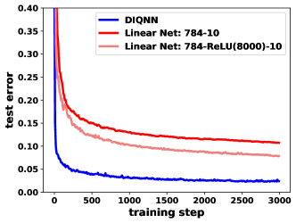
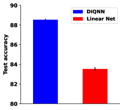
Figure 1: Performance of DIQNN. Left: Test error curves on MNIST. Right: Test accuracy (with error bar) on FMNIST.

FMNIST results. We employ a two-layer convolutional neural network (CNN), comprising of one convolution layer with ReLU activation function and one fully connected layer. We examine whether the classifier ( the fully connected layer) is linear or quadratic. The test accuracy of these two models is presented in the right figure of Figure 1, indicating that DIQNN significantly outperforms the linear net.

3.2 Low rank properties of DIQNN

Although quadratic classifiers offer advantages, their computational cost is large. Therefore, it is imperative to reduce the number of trainable parameters while preserving the quadratic form in DIQNN. To this end, we want to find out whether the trained network can possess some good properties. Firstly, the weight matrix $A$ undergoes spectrum decomposition. The decomposition can be represented as follows:

$$A=\sum_{i=1}^{n}\lambda_{i}\mathbf{a}_{i}\mathbf{a}_{i}^{T},\ |\lambda_{1}|\geq|\lambda_{2}|\geq|\lambda_{3}|\geq\cdots\geq|\lambda_{n}|$$ (2)

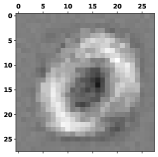
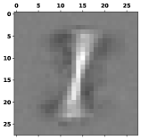
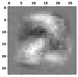
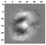
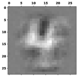
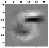
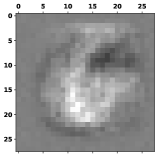
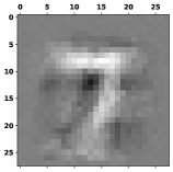
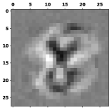
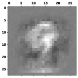
Figure 2: The leading eigenvectors of different after-trained weight matrices.(Totally 10 weight matrices)

Here, numerical experiment is conducted on MNIST. Figure 2 illustrates the leading eigenvectors of different after-train weight matrices. It can be observed that these vectors are similar to the spike-triggered average of output neurons. The term "spike-triggered average" refers to the average input that evokes the highest response from a neuron[22]. This phenomenon implies the majority of information in spike-triggered average could be encoded by the leading eigenvector of the weight matrix $A$. In addition, we find when only the first few eigenvectors are kept in weight matrix $A$, DIQNN can achieve high test accuracy. Experiments on FMNIST exhibit similar results. Additional details are provided in supplementary materials. These observations suggest that DIQNN naturally display low-rank properties after training.

4 Low-Rank DIQNN

The low-rank property of DIQNN allows us to explicitly set the weight matrix $A$ in the form of a sum of rank-one matrices given by the following equation:

$$A=\sum_{i=1}^{r}\mathbf{c}_{i}\mathbf{c}_{i}^{T}$$ (3)

where $r$ is a hyperparameter and $\mathbf{c}_{i}$ is a column vector. We refer to this model as Low-Rank DIQNN owing to its capability of reducing computational cost, since $r$ is always small in comparison to the dimension of weight matrix $A$.

4.1 Performance of Low-Rank DIQNN on classification tasks

We next investigate the performance of Low-Rank DIQNN on MNIST, FMNIST, and CIFAR-10. The details of the numerical experiments and results on other datasets such as Iris are provided in supplementary materials.

MNIST and FMNIST results. We utilize the same network structure as in the previous section for Low-Rank DIQNN. On MNIST, we employ single-layer Low-Rank DIQNNs with various ranks, while on FMNIST, we utilize a two-layer convolutional neural network that contains one low-rank classifier.

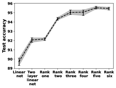
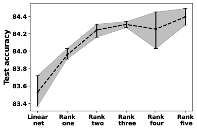
Figure 3: Performance of Low-Rank DIQNN. Left: On MNIST. Right: On FMNIST.

Figure 3 mainly compares linear net with Low-Rank DIQNN having various ranks. The figure shows that when Low-Rank DIQNN with just one rank ($r=1$ in equation 3) performs better than the linear net, even though they have an equal number of trainable parameters (Low-Rank DIQNN with one rank even outperforms a two-layer linear net with ReLU activation function). Moreover, as the number of ranks in Low-Rank DIQNN increases, its performance continues to improve until it almost reaches saturation.

Table 3: Performance of Low-Rank DIQNN on CIFAR-10.

Network structure	Residual blocks	Last layer method (Classifier)	Test accuracy
ResNet 10	[1,1,1,1]	Linear Rank one Rank two Rank three Rank four	92.20$\pm$0.11$\%$ 92.32$\pm$0.18$\%$ 92.35$\pm$0.09$\%$ 92.48$\pm$0.07$\%$ 92.50$\pm$0.11$\%$
ResNet 12	[2,1,1,1]	Linear Rank one Rank two Rank three Rank four	92.59$\pm$0.14$\%$ 92.63$\pm$0.15$\%$ 92.76$\pm$0.08$\%$ 92.72$\pm$0.15$\%$ 92.89$\pm$0.14$\%$
ResNet 14	[2,2,1,1]	Linear Rank one Rank two Rank three Rank four	92.82$\pm$0.20$\%$ 93.00$\pm$0.07$\%$ 92.89$\pm$0.17$\%$ 93.30$\pm$0.12$\%$ 93.31$\pm$0.19$\%$
ResNet 16	[2,2,2,1]	Linear Rank one Rank two Rank three Rank four	93.27$\pm$0.08$\%$ 93.26$\pm$0.04$\%$ 93.29$\pm$0.05$\%$ 93.33$\pm$0.17$\%$ 93.43$\pm$0.05$\%$
ResNet 18	[2,2,2,2]	Linear Rank one Rank two Rank three Rank four	93.51$\pm$0.04$\%$ 93.46$\pm$0.13$\%$ 93.57$\pm$0.03$\%$ 93.67$\pm$0.13$\%$ 93.66$\pm$0.06$\%$

CIFAR-10 results. We train ResNets[8] with a low-rank classifier on CIFAR-10. Similar to the CNN used in FMNIST, we keep the computation of convolution layers in ResNet intact, and only modify the last fully connected layer to low-rank form. Test accuracy results on different ResNets are presented in Table 3, where the "Residual blocks" column means how these ResNets are constructed in terms of their convolution layers [8]. Similar to the results on MNIST and FMNIST, it is evident that Low-Rank DIQNN performs better than traditional ANN, and its performance increases with higher ranks.

4.2 Analyzing generalization of Low-Rank DIQNN on classification tasks

This section begins by defining the margin on Low-Rank DIQNN. We then utilize it to analyze Low-Rank DIQNN and show the consistency between generalization and our margin. Finally, we show this margin can be used to accelerate the change of test accuracy in Low-Rank DIQNN. The details of the numerical experiments and the proof of our theorem are provided in supplementary materials.

4.2.1 Normalized margin

Given training dataset $\{(x_{n},y_{n})\}_{n=1}^{N}$, each data point $x_{n}\in\mathbb{R}^{d}$ has a true label $y_{n}\in[k]$, where $k$ ($k\geq 2$) denotes the total number of classes. Given a certain input $x_{n}$, the Low-Rank DIQNN produces an output vector $\Phi(x_{n},\theta)\in\mathbb{R}^{k}$, where $\theta$ represents the trainable network parameters. Naturally, the margin for data point $x_{n}$ can be defined as $s_{n}=(\Phi(x_{n},\theta))_{y_{n}}-(\Phi(x_{n},\theta))_{j},\ j=\arg\max_{i\neq y_{n}}{(\Phi(x_{n},\theta))_{i}}$. However, this definition does not directly reflect the distance between data point $x_{n}$ and the classification boundary of the model in input space since it does not obey scale invariance. To address this issue, we propose a normalized margin for single data point $x_{n}$: $\frac{s_{n}}{\|\Phi(x_{n},\theta)\|_{2}}$, and the average of this margin across all training data points are taken into consideration:

$$\frac{1}{N}\sum^{N}_{n=1}\frac{s_{n}}{\|\Phi(x_{n},\theta)\|_{2}}=\frac{1}{N}\sum^{N}_{n=1}\frac{(\Phi(x_{n},\theta))_{y_{n}}}{\|\Phi(x_{n},\theta)\|_{2}}-\frac{1}{N}\sum^{N}_{n=1}\ \frac{(\Phi(x_{n},\theta))_{j}}{\|\Phi(x_{n},\theta)\|_{2}}\triangleq\mu_{1}-\mu_{2}\triangleq\Delta\mu$$ (4)

4.2.2 XOR problem

We employ a single-layer Low-Rank DIQNN with one rank to solve the XOR problem and prove the following theorem (see details in supplementary materials):

Theorem 1.

Training single layer Low-Rank DIQNN with one rank to solve XOR problem under cross-entropy loss $\mathcal{L}(\theta_{t})$ and gradient flow algorithm as $\frac{d\theta_{t}}{dt}=-\nabla_{\theta}\mathcal{L}(\theta_{t})$, we have:

$$\frac{d\Delta\mu}{dt}>0\ \ \text{and}\ \lim_{t\rightarrow\infty}\Delta\mu=1.$$

With our defined margin, the above theorem demonstrates that our margin will monotonically increase and finally reach its maximum value. Notably, in Low-Rank DIQNN, one can prove $-1\leq\Delta\mu\leq 1$.

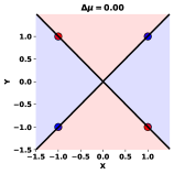
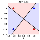
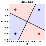
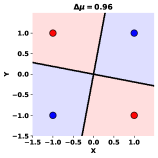
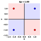
Figure 4: Training process (gradient descent) of single layer Low-Rank DIQNN with one rank on XOR problem. From left to right: Initialization, after 12, 36, 84, 396 training steps, respectively. The blue region indicates the model’s classification for the blue class, while the red region indicates classification for the red class. And the title of each picture indicates the value of our margin $\Delta\mu$ at different training steps.

We perform numerical experiments, as shown in Figure 4. These figures display the training dynamics with gradient descent (GD). It shows that our margin reflects the relative distance between data points and the classification boundary. And we observe that Low-Rank DIQNN can achieve a smaller generalization error by pushing the classification boundary further away from data points until it converges to an optimal result, which aligns with our theorem. Therefore, our theorem implies that Low-Rank DIQNN reduces generalization error monotonically until converging to the optimal solution.

4.2.3 General set up

We next extend our investigation to general datasets and training algorithms (e.g., stochastic gradient descent (SGD)).

Definition 1.

(Homogeneous property) We say a network satisfy the homogeneous property for some integer $L$ if:

$$\Phi(x_{n},\theta_{t})=\|\theta_{t}\|_{2}^{L}\Phi(x_{n},\frac{\theta_{t}}{\|\theta_{t}\|_{2}})$$

Lemma 1.

(Homogeneous property) Low-Rank DIQNN satisfy the homogeneous property: $\Phi(x_{n},\theta_{t})=\|\theta_{t}\|_{2}^{L}\Phi(x_{n},\frac{\theta_{t}}{\|\theta_{t}\|_{2}})$ for $L=2^{l+1}-2$, where $l$ is the total number of layers of Low-Rank DIQNN. Moreover, we can prove that $\langle\partial_{\theta}(\Phi(x_{n},\theta_{t}))_{i},\theta_{t}\rangle=L(\Phi(x_{n},\theta_{t}))_{i}$ $\forall i\in[k]$

Definition 2.

A set that consist of real numbers $\{y_{1},y_{2},\cdots,y_{m}\}$ satisfy the $\varepsilon-$separated condition if $y_{j}-\min_{i}(y_{i})\geq 1/\varepsilon,\forall j\in[m],j\neq\arg\min_{i}(y_{i})$

Definition 3.

$s_{nj}=(\Phi(x_{n},\theta_{t}))_{y_{n}}-(\Phi(x_{n},\theta_{t}))_{j}$; $j_{n}=\arg\max_{i\neq y_{n}}{(\Phi(x_{n},\theta))_{i}}$; $s_{n}=s_{nj_{n}}$; $c$ is the condition number of matrix $A=\partial_{\theta}S\partial_{\theta}S^{T}-\frac{L^{2}}{\|\theta_{t}\|_{2}^{2}}SS^{T}$, where $S=(s_{1},\dots,s_{n})^{T}$, $\partial_{\theta}S=(\partial_{\theta}s_{1},\dots,\partial_{\theta}s_{n})^{T}$; $\mathbf{v}=(v_{1},\dots,v_{N})^{T}$, where $v_{n}=\frac{e^{(\Phi(x_{n},\theta_{t}))_{j_{n}}}}{\sum_{i=1}^{k}e^{(\Phi(x_{n},\theta_{t}))_{i}}}$, it should be noted that all of these values or vectors are time dependent.

Theorem 2.

Training Low-Rank DIQNN under cross-entropy loss and gradient flow algorithm, if the following three assumptions are satisfied in a small time interval $[t-\Delta t,t+\Delta t]$ for some $\Delta t>0$:

• $\|\Phi(x_{n},\theta_{t})\|_{2}=a_{n}\|\theta_{t}\|_{2}^{L}$

• The set $\{s_{nj}\}_{j=1,j\neq y_{n}}^{k}$ satisfy the $\varepsilon-$separated condition for some $\varepsilon>0$ ($\forall n\in[N]$), and $\{\|\partial_{\theta}s_{nj}\|_{2}\}_{n\in[N],j\in[k]}$ is uniformly bounded with some constant $M$.

• $c-1\leq\frac{2m}{\sqrt{1-m^{2}}}$, where $m=\cos(\mathbf{a},\mathbf{v})>0$, $\mathbf{a}=(1/a_{1},\dots,1/a_{N})^{T}$

Then at time $t$ we have:

$$\frac{d\Delta\mu}{dt}\geq-\frac{M^{2}(k-2)\|\mathbf{a}\|_{1}}{N\|\theta_{t}\|_{2}^{L}}e^{-\frac{1}{\varepsilon}}.$$

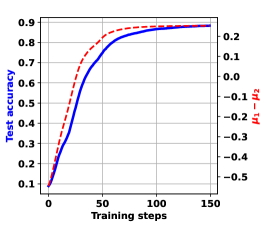
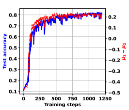
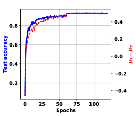
Figure 5: Numerical experiments on MNIST(Left), FMNIST(Middle) and CIFAR-10(Right). There are two vertical axes: the left axis represents the test accuracy, and the right axis represents our margin $\Delta\mu$. The blue solid line indicates test accuracy while the red dash line indicates our margin.

This theorem indicates that through the training process, our defined margin increases in an almost monotonic manner

We next perform numerical experiments on MNIST, FMNIST, and CIFAR-10 with SGD training algorithm, as shown in Figure 5. These figures demonstrate that the margin increases almost monotonically on these datasets, which is consistent with our theorem. Additionally, it is noteworthy that the dynamics of the margin is closely related to that of test accuracy, indicating that the margin well reflects the generalization error of Low-Rank DIQNN. Our theorem implies that the generalization error decreases monotonically, indicating the Low-Rank DIQNN is approaching the solution with good generalization.

The monotonical increase of our margin during training process may imply the existence of implicit regularity. Therefore, we next explore the impact of explicitly adding margin regularization to the loss function. The modified loss function is given as follows:

$$\bar{\mathcal{L}}(\theta)=\mathcal{L}(\theta)-\lambda*\Delta\mu,$$ (5)

where $\mathcal{L}(\theta)$ is the original cross-entropy loss, and $\lambda$ is a hyperparameter that controls the magnitude of regularization. Numerical results on MNIST, FMNIST, and CIFAR-10 are provided in Figure 6. It is found that the convergence speed is indeed enhanced after the margin regularization is added, here the convergence speed is characterized by the test accuracy, since one cares more about the generalization capability of solutions. This indicates one can obtain a solution with small generalization error in a short time by explicitly adding margin regularization.

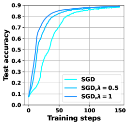
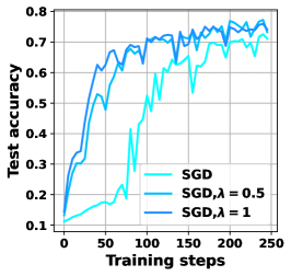
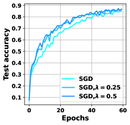
Figure 6: Test accuracy curves on datasets: MNIST(Left), FMNIST(Middle) and CIFAR-10(Right), respectively, with loss function given in equation 5.

5 Conclusion

In this paper, we present a novel ANN model inspired by the quadratic integration rule of dendrite, namely DIQNN, which significantly outperforms traditional ANNs. Based on observations of the low-rank structure of DIQNN, we propose Low-Rank DIQNN that retains the high performance while having low computational cost. Moreover, we provide a theoretical framework to analyze the generalization error in classification tasks, and experimental results on MNIST, FMNIST, and CIFAR-10 exhibit the effectiveness of our framework. Considering quadratic integration rule of neurons could be confined to a few brain areas[7], thus other integration rules of neurons may be discovered in future electrophysiological experiments. Our framework could be extended to design brain-inspired ANN models that can incorporate these new integration rules. Moreover, in the design of brain-inspired deep neural networks, it might be possible to refer to our framework to incorporate different integration rules in different layers, which represent neurons in various brain areas. Additionally, how to theoretically analyze the above brain-inspired models developed from new integration rules will also be an important issue. It is expected to extend our margin theory to investigate the generalization error of these new brain-inspired models in classification tasks.

References

- Bu and Karpatne [2021] Jie Bu and Anuj Karpatne. Quadratic residual networks: A new class of neural networks for solving forward and inverse problems in physics involving pdes. In SDM, 2021.
- Chavlis and Poirazi [2021] Spyridon Chavlis and Panayiota Poirazi. Drawing inspiration from biological dendrites to empower artificial neural networks. Current Opinion in Neurobiology, 70:1–10, 2021.
- DeClaris and Su [1991] Nicholas DeClaris and Min Su. A novel class of neural networks with quadratic junctions. Conference Proceedings 1991 IEEE International Conference on Systems, Man, and Cybernetics, pages 1557–1562 vol.3, 1991.
- Fan et al. [2017] Fenglei Fan, Wenxiang Cong, and Ge Wang. A new type of neurons for machine learning. International Journal for Numerical Methods in Biomedical Engineering, 34, 2017.
- Goyal et al. [2020] Mohit Goyal, Rajan Goyal, and Brejesh Lall. Improved polynomial neural networks with normalised activations. 2020 International Joint Conference on Neural Networks (IJCNN), pages 1–8, 2020.
- Guo and Zhang [2021] Yiwen Guo and Changshui Zhang. Recent advances in large margin learning. IEEE Transactions on Pattern Analysis and Machine Intelligence, 44:7167–7174, 2021.
- Hao et al. [2009] Jiang Hao, Xu-Dong Wang, Yang Dan, Mu ming Poo, and Xiaohui Zhang. An arithmetic rule for spatial summation of excitatory and inhibitory inputs in pyramidal neurons. Proceedings of the National Academy of Sciences, 106:21906 – 21911, 2009.
- He et al. [2015] Kaiming He, X. Zhang, Shaoqing Ren, and Jian Sun. Deep residual learning for image recognition. 2016 IEEE Conference on Computer Vision and Pattern Recognition (CVPR), pages 770–778, 2015.
- Jiang et al. [2019] Yiyang Jiang, Fan Yang, Hengliang Zhu, Dian Zhou, and Xuan Zeng. Nonlinear cnn: improving cnns with quadratic convolutions. Neural Computing and Applications, 32:8507–8516, 2019.
- Jones and Kording [2021] Ilenna Simone Jones and Konrad Paul Kording. Might a single neuron solve interesting machine learning problems through successive computations on its dendritic tree? Neural Computation, 33:1554–1571, 2021.
- Kobayashi [2019] Takumi Kobayashi. Large margin in softmax cross-entropy loss. In British Machine Vision Conference, 2019.
- LeCun and Cortes [2005] Yann LeCun and Corinna Cortes. The mnist database of handwritten digits. 2005.
- Li et al. [2014] Songting Li, Nan Liu, Xiaohui Zhang, Douglas Zhou, and David Cai. Bilinearity in spatiotemporal integration of synaptic inputs. PLoS Computational Biology, 10, 2014.
- Liu and Wang [2020] Gang Liu and Junchang Wang. Dendrite net: A white-box module for classification, regression, and system identification. IEEE Transactions on Cybernetics, 52:13774–13787, 2020.
- Lyu and Li [2020] Kaifeng Lyu and Jian Li. Gradient descent maximizes the margin of homogeneous neural networks. In International Conference on Learning Representations, 2020.
- Mantini and Shah [2021] Pranav Mantini and Shishir K. Shah. Cqnn: Convolutional quadratic neural networks. 2020 25th International Conference on Pattern Recognition (ICPR), pages 9819–9826, 2021.
- Moldwin et al. [2021] Toviah Moldwin, Menachem Kalmenson, and Idan Segev. The gradient clusteron: A model neuron that learns to solve classification tasks via dendritic nonlinearities, structural plasticity, and gradient descent. PLoS Computational Biology, 17, 2021.
- Moosavi-Dezfooli et al. [2015] Seyed-Mohsen Moosavi-Dezfooli, Alhussein Fawzi, and Pascal Frossard. Deepfool: A simple and accurate method to fool deep neural networks. 2016 IEEE Conference on Computer Vision and Pattern Recognition (CVPR), pages 2574–2582, 2015.
- Ojha and Nicosia [2022] Varun Kumar Ojha and Giuseppe Nicosia. Backpropagation neural tree. Neural networks : the official journal of the International Neural Network Society, 149:66–83, 2022.
- Payeur et al. [2020] Alexandre Payeur, Jordan Guerguiev, Friedemann Zenke, Blake A. Richards, and Richard Naud. Burst-dependent synaptic plasticity can coordinate learning in hierarchical circuits. Nature Neuroscience, 24:1010 – 1019, 2020.
- Redlapalli et al. [2003] S. Redlapalli, M.M. Gupta, and Kim Yong Song. Development of quadratic neural unit with applications to pattern classification. Fourth International Symposium on Uncertainty Modeling and Analysis, 2003. ISUMA 2003., pages 141–146, 2003.
- Schwartz et al. [2006] Odelia Schwartz, Jonathan W. Pillow, Nicole C. Rust, and Eero P. Simoncelli. Spike-triggered neural characterization. Journal of vision, 6 4:484–507, 2006.
- Sokolić et al. [2017] Jure Sokolić, Raja Giryes, Guillermo Sapiro, and Miguel R. D. Rodrigues. Robust large margin deep neural networks. IEEE Transactions on Signal Processing, 65:4265–4280, 2017.
- Spruston [2008] Nelson Spruston. Pyramidal neurons: dendritic structure and synaptic integration. Nature Reviews Neuroscience, 9:206–221, 2008.
- Ujfalussy et al. [2018] Balázs B. Ujfalussy, Judit K. Makara, Máté Lengyel, and Tiago Branco. Global and multiplexed dendritic computations under in vivo-like conditions. Neuron, 100:579 – 592.e5, 2018.
- Wu and Yu [2019] Kaiwen Wu and Yaoliang Yu. Understanding adversarial robustness: The trade-off between minimum and average margin. ArXiv, abs/1907.11780, 2019.
- Wu et al. [2018] Xundong Wu, Xiangwen Liu, Wei Li, and Qing Wu. Improved expressivity through dendritic neural networks. In Neural Information Processing Systems, 2018.
- Xiao et al. [2017] Han Xiao, Kashif Rasul, and Roland Vollgraf. Fashion-mnist: a novel image dataset for benchmarking machine learning algorithms. ArXiv, abs/1708.07747, 2017.
- Xu et al. [2022] Zirui Xu, Fuxun Yu, Jinjun Xiong, and Xiang Chen. Quadralib: A performant quadratic neural network library for architecture optimization and design exploration. Proceedings of Machine Learning and Systems, 4:503–514, 2022.
- Yan et al. [2018] Ziang Yan, Yiwen Guo, and Changshui Zhang. Deep defense: Training dnns with improved adversarial robustness. In Neural Information Processing Systems, 2018.
- Zoumpourlis et al. [2017] Georgios Zoumpourlis, Alexandros Doumanoglou, Nicholas Vretos, and Petros Daras. Non-linear convolution filters for cnn-based learning. 2017 IEEE International Conference on Computer Vision (ICCV), pages 4771–4779, 2017.