Object-based Probabilistic Similarity Evidence of Sparse Latent Features from Fully Convolutional Networks

Abstract

Similarity analysis using neural networks has emerged as a powerful technique for understanding and categorizing complex patterns in various domains. By leveraging the latent representations learned by neural networks, data objects such as images can be compared effectively. This research explores the utilization of latent information generated by fully convolutional networks (FCNs) in similarity analysis, notably to estimate the visual resemblance of objects segmented in 2D pictures. To do this, the analytical scheme comprises two steps: (1) extracting and transforming feature patterns per 2D object from a trained FCN, and (2) identifying the most similar patterns through fuzzy inference. The step (2) can be further enhanced by incorporating a weighting scheme that considers the significance of latent variables in the analysis. The results provide valuable insights into the benefits and challenges of employing neural network-based similarity analysis for discerning data patterns effectively.

1. Introduction

Computer vision and image analysis have gained significant importance in various research fields. Imagery data often contain multiple 2D objects that need to be accurately depicted and organized, enabling the study of unknown patterns or targeted object retrieval (e.g., [1, 2, 3]). Similarity analysis plays a crucial role in such study. By comparing the resemblance of image components, the identification of recurring structures or visual relationships becomes possible. In practice, this comparison can involve transforming the image components into a vector space and utilizing specific metrics like distance, inner product, or entropy measures [4] for comparing vector elements. While feature vectors translate object properties from image sets, they can be estimated via computational methods that learn to discern visual features at the pixel level. Deep learning using neural networks has particularly advanced this area, enabling remarkable progress in object recognition across diverse aspects and distortions [5, 6]. The generalization ability of such networks makes it possible to extract spatial details into semantic information that can be exploited for similarity analysis. Notably, Siamese networks have been widely used for this task [7, 8, 9]. They learn similarity or dissimilarity between pairs of inputs by using twin neural networks with shared weights to extract features from two input samples, and then compare the feature representations to compute a similarity or dissimilarity score. Triplet network is another approach [10, 11] where embeddings are learnt using triplets of samples consisting of an anchor, a positive (similar) example, and a negative (dissimilar) example to train the network. While training, the distance between similar samples is minimized and dissimilar samples are maximized. Another method is deep metric learning, which tackles similarity analysis tasks by learning a feature embedding space where similar samples are closer to each other, and dissimilar samples are farther apart [12, 13]. It typically involves training a neural network to optimize a similarity or distance metric loss function.

While these learning techniques utilize neural networks for similarity analysis, they need to be optimized for distinct aspects of similarity. In contrast, this research aims to demonstrate the effectiveness of utilizing features extracted from pre-trained networks for similarity analysis without relying on a specific loss criterion for such task. The proposed analytical approach consists of two steps: (1) optimizing the network's feature representativeness during training, and (2) leveraging the learned embeddings post-training via a mathematical approach. Using a collection of images, the learning model captures the visual properties of 2D objects identified in each image. Techniques like increasing network sparsity at the channel level, i.e., reducing the number of network features, can be employed to enhance feature quality during the model training. Subsequently, these features are extracted, transformed, and compared through a mathematical procedure.

One commonly used learning model is the fully convolutional network (FCN) [14], which can capture high-level abstractions of images via convolutions. Since a convolution operation is a mathematic approximation of the activity of a neuron (stimulus) within its receptive field [6], stimuli for each hidden unit can presumably respond to an object(s) of interest in the original data space (noted $\mathcal{X}$) that we eventually attempt to segment from the last layer of FCNs. Stimuli patterns for a single prediction class can be multiple, i.e., the network determines diverse feature patterns learned for the corresponding class. An example is shown by [15] who clustered various latent patterns from an FCN considering a one-class segmentation problem i.e., a main object class, and a sub-class being a chunk of the main one for detailing the similarity analysis and resulting clusters. They demonstrated that a significant portion of the encoding-decoding activation space of the trained FCN (noted $\mathcal{A}$) exhibits multimodality. By leveraging the multimodality of convolutional maps, new possibilities for object-oriented similarity analysis can be unlocked.

This paper focuses on conducting a similarity analysis of objects determined by FCNs. The approach complements the work presented in [15], which demonstrated the potential of leveraging feature patterns learned from a supervised segmentation model for object categorization. This can be done without learning a latent space specifically for a similarity analysis (or clustering) task when mapping $\mathcal{X}$ to a new space. In this context, an FCN is trained to address a one-class segmentation problem, and then, similarity of segmentation is measured in a second step, conducted post-training. Results of this segmentation are used to extract activated regions of network feature maps associated to object segments. As described in [15] the extraction procedure considers the backward propagation of a one-class segmentation mask throughout the network to extract sub-regions of $N$ activated feature maps $F=\left\{f_{1},\ldots,f_{N}\right\}$ where, layer-per-layer, representation sets $M=\left\{m_{1},\ldots,m_{N}\right\}$, locally responsive to the respective one-class segment in $F$ are collected. On this basis, [15] revealed groups of similar feature patterns by (1) taking the mean value (or magnitude) of elements of $M_{i}$ to compose a (mean) activation vector $v_{i}=(x_{i,1},\ldots,x_{i,N})$ associated to an $i$th segmented object, then (2) comparing feature vectors of multiple objects by correlation analyses, and (3) clustering hierarchically these vectors based on correlation results. Resulting clusters, i.e., groups of similar segments, or objects extracted from $\mathcal{X}$, were evaluated visually, but the measure of similarity from $v_{i}$ among objects of a same cluster was done in a Euclidean space. In this case, the evaluation of similarity (in the semantic sense) shall require estimating the distance of pairs of vectors for which we know the meaning. This is a difficult task because a cluster is specified by analogous latent features whose meanings are unknown. From a statistical standpoint, it is however possible to quantify this similarity for more interpretable and guided object identification. To address this, a probabilistic similarity measure of $v_{i}$ is proposed in this study, by employing fuzzy partitioning of the latent domain $\mathcal{A}$ using fuzzy sets. Technically, the pattern of a reference object $q$ (query), denoted as $v_{q}$, is collected, and the proximity of its components to those of $v_{i}$, for any object indexed $i$ in a set of segmented objects $O$, is evaluated. An element $x_{i,j}\in v_{i}$ is thus evaluated in local neighborhoods of an element $x_{q,j}\in v_{q}$. As this neighborhood is fuzzy, we determine the probabilistic “distance” between these elements using a membership function (e.g., Gaussian function). The degree of fuzziness of any feature vector $v_{i}$, with respect to $v_{q}$, forms the basis of similarity search. An efficient way to explore analogous patterns is to rank $v_{i}$ by order of similarity ($\forall i\in O$) with respect to a queried object indexed $q$.

In this research, the objective is to tackle the calculation of similarity scores between feature patterns through fuzzy inference. The methodology is exemplified by utilizing a standard FCN, such as U-Net [16], which is capable of learning sparse semantic representations. This model is trained using the UT Zappos50k datasets [17], consisting of 12,833 images of boots, all of the same dimension and orientation (see examples in Fig.1). Sparsity is generated at the channel level, and implemented for dimensionality reduction of patterns extracted from $\mathcal{A}$, which are used in similarity computations. A term enforcing sparsity is added to the loss to set several (activated) convolution outputs to zero. After training, the extraction and transformation procedures mentioned earlier are employed to construct $O$ and its corresponding feature vectors. Subsequently, the "inactive" features, along with unimportant ones, are pruned using eigen decomposition. The remaining "active" features (not pruned) are processed for similarity computation of the feature vectors. The approach will be optimized through the presentation of learning metrics. Additionally, the similarity search scheme will be tested using features extracted from a non-FCN model, ResNet50 [18], which is trained on the MNIST dataset.

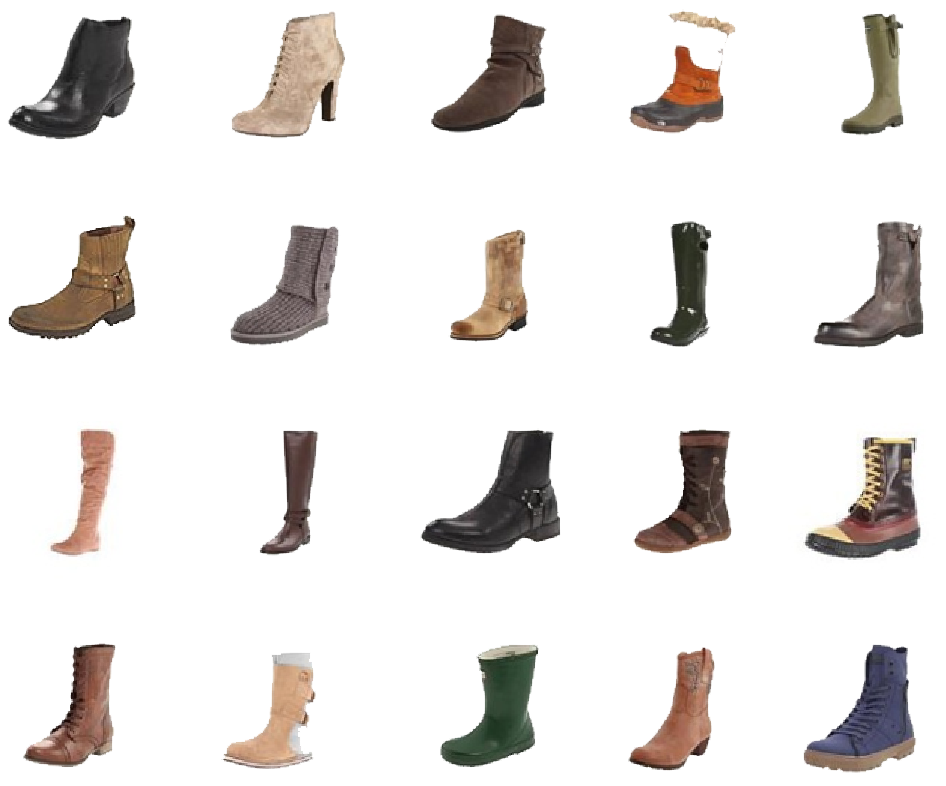
Figure 1: Examples of objects studied for similarity.

2. Similarity evidence of segmentation

2.1. Feature extraction and pruning

Consider a trained FCN noted $U$ with a set of selected layers $\phi$ consisting of $N$ features, and an extraction procedure applied to a one-class segmentation problem, where a single object is segmented per image. To an object in $\mathcal{X}$ corresponds a predicted set of pixels (segment) generated by $U$ in its last convolution layer (output). Let $f_{j}$ be an activated feature map of $\phi$, which constitutes the set $F\ (\forall j\leq N$). From this map, there exists a set of pixels $m_{i,j}$ responsive to an object $i$ from $\mathcal{X}$ i.e., only a specific part of $f_{j}$ is activated with respect to an $i$th segment of an input image. The activated pixels $m_{i,j}$ are first extracted by cropping the segment $i$ from the last layer of $U$, then propagating the cropped region from segmentation to a specified $f_{j}$ in $\phi$ by re-adjusting it with regards to the dimensions of $f_{j}$ i.e., both, the centroid position and size of the cropped segment region is adapted to the resolution of lower-level feature maps. For instance, the propagation from an output with size $256\times 256$, to a feature map of size $128\times 128$ requires dividing the cropping size (and its centroid coordinates) by 2. Note that due to spatial reduction and invariance, the pixel-wise information of the original image object is altered in the network after passing a filter over outputs with a given pixel shifting (stride). Usually, convolutional layers pad the feature map if the convolution crosses the output borders, which triggers a shift of the activated signal. However, much of this signal (and position) can be maintained within the propagating window using small and symmetric kernels for convolution, pooling and up-sampling operations, and if padding does not add up significant information on the edge of the outputs, which is the case for the network used in this study (see Section 3.1).

Assuming $M_{i}=\left\{m_{i,1},\ldots,m_{i,N}\right\}$ a set of extracted features derived from $F$, a $N$-dimensional feature vector $v_{i}$ is first generated after describing every element of $M_{i}$ statistically. For example, the first statistical moment (mean) of $m_{i,j}$ is calculated, and can be regarded as an activation magnitude noted $x_{i,j}$. Accordingly, two objects with same or very similar characteristics in $\mathcal{X}$ presumably yield analogous representations $v_{i}$ in $\mathcal{A}$ i.e., corresponding features $m_{i,j}$ have similar magnitudes. This assumption holds when objects from $\mathcal{X}$ are of the same dimension, ensuring that pattern comparisons via $v_{i}$ are size invariant. The data utilized in this research exhibits this characteristic, as presented in Fig.1. Therefore, for each $i$th object segmented by $U$ from the image dataset UT Zappos50k (with size $s=|O|$), the feature matrix denoting $M$ can be represented as $X$. Each column $u_{j}$ in $X$ corresponds to a feature vector with a probability density function (PDF) defined as $p_{u_{j}}$. Additionally, the row $v_{i}=(x_{i,1},\ldots,x_{i,N})$ in $X$ corresponds to the feature vector or latent pattern of the $i$th object. For similarity purpose, if we were to compare multiple patterns, it may be convenient to reduce the dimensionality of $X$. In this study, sparse learning is employed to decrease the number of exploitable (activated) features in $\mathcal{A}$ during training (see method in Appendix A). Subsequently, singular-value decomposition (SVD) is applied to approximate the representation of $X$, obtained after training, by decomposing it into orthogonal and diagonal components, such that

$$X_{s\times N} =T_{s\times s}\Sigma_{s\times N}V_{N\times N}^{T},$$ (1)

where $s=|O|$. $T$ and $V$ are orthonormal matrices comprising singular vectors, which make up the columns of $T$ and rows of $V^{T}$. $\Sigma$ is a rectangular diagonal matrix whose diagonal elements are positive singular values arranged in decreasing order. Here, only a subset of relevant features can be determined by retaining 99% of data variance from the activation magnitudes in $X$. The first (and highest) singular value in $\Sigma$ is considered because its first component accounts for the majority of the variances in $X$. Hence, the first singular vector of $V^{T}$ is taken as a basis vector to rank and withhold the $n$ most relevant features ($n<N$). The resulting network-related data matrix is noted as $X^{{}^{\prime}}\in\mathbb{R}^{s\times n}$, with $n$ being the number of withheld activation magnitudes after pruning the $N$ total network features collected from $\phi$. The $i$th mean activation vector is defined as $v_{i}=\left(X_{i,j}^{{}^{\prime}}\right)_{1\leq j\leq n}=(x_{i,1},\ldots,x_{i,n})$, and the components of the $j$th feature vector $u_{j}=\left(X_{i,j}^{{}^{\prime}}\right)_{1\leq i\leq s}=(x_{1,j},\ldots,x_{s,j})$ are evaluated for similarity purpose.

2.2. Probabilistic transformation

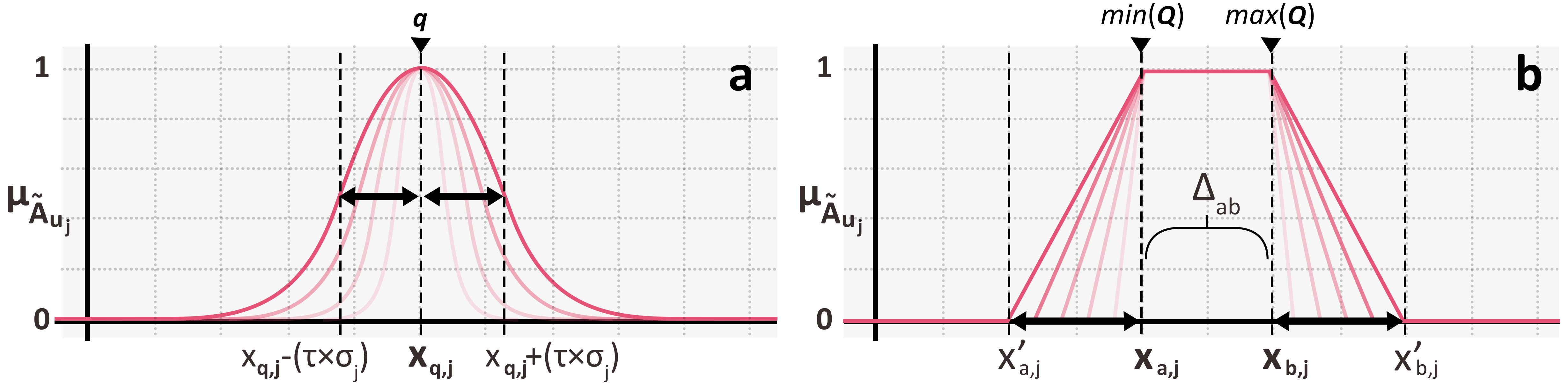
Figure 2: Membership functions: (a) Gaussian type, with $x_{q,j}$ the central value of a $j$th feature given a query $q$, and $\sigma_{j}$ the standard deviation, and (b) trapezoidal, for a set of queries Q, with the lower and upper limits defined by $x^{{}^{\prime}}_{a,j}=x_{a,j}-\Delta_{ab}$, and $x^{{}^{\prime}}_{b,j}=x_{b,j}+\Delta_{ab}$, respectively. $\Delta_{ab}$ is the range between the support limits $x_{a,j}$ and $x_{b,j}$, and $\tau\in[0,1]$ is an arbitrary factor. Dark arrows indicate the varying uncertainty limits modulated by $\tau$.

Consider two objects collected from $O$ with similar characteristics in $\mathcal{X}$: an object indexed $q$ that we wish to study (a query) and an object indexed $i$ selected for comparison. Presumably, their feature patterns may be analogous i.e., the activation magnitudes $x_{i,j}$ of related feature vectors ($v_{i}$ and $v_{q}$) shall be close. Given this assumption, we can denote a confidence interval of values possibly determining $v_{q}$, centered at a point estimate $x_{q,j}$ in $p_{u_{j}}$. From a probabilistic perspective, this confidence interval is fuzzy, meaning that as adjacent values approach $x_{q,j}$, the probability of determining $v_{q}$ increases. This fuzziness can be measured using a membership function $\mu_{{\widetilde{A}}_{u_{j}}\ }$, which transforms $u_{j}$ into a fuzzy set ${\widetilde{A}}_{u_{j}}$. The choice of $\mu_{{\widetilde{A}}_{u_{j}}}$ depends on the a priori knowledge of data from the practitioner, or the type of object query desired. For instance, utilizing a Gaussian membership function enables obtaining ${\widetilde{A}}_{u_{j}}$ using the equation

$$\mu_{{\widetilde{A}}_{u_{j}}}^{q}\left(x_{i,j}\right)=e^{-\left(\frac{x_{i,j}-x_{q,j}}{\tau\sigma_{j}}\right)^{2}},$$ (2)

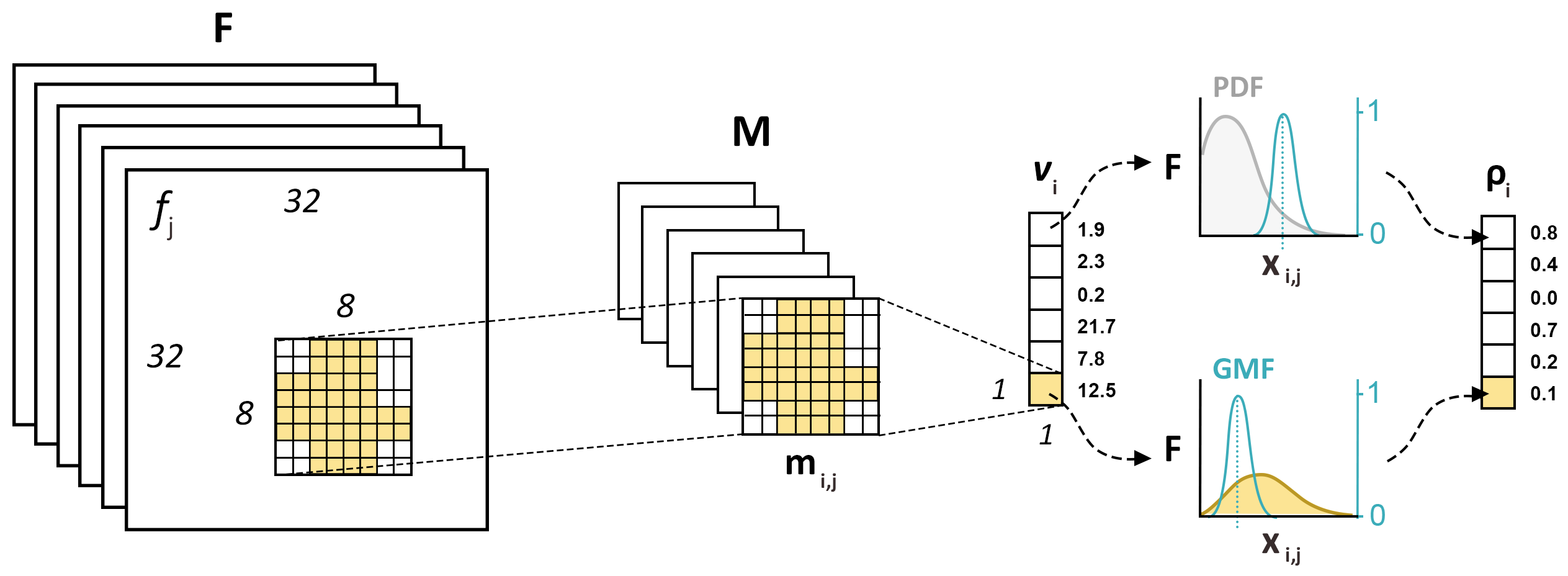
Figure 3: Object-oriented extraction of feature $m_{i,j}$ from an activated feature $f_{j}$. Resulting set $M$ is converted into an activation vector $v_{i}$ by statistical description of the activated region of $m_{i,j}$ (yellow mask). Each component $x_{i,j}\in v_{i}$, associated to a feature $f_{j}$, defines a probability density function (PDF) computed for a collection of objects ($\forall i\in O$). A sampled value of this PDF, specified by a query $q$, corresponds to the centroid (mean) of a Gaussian membership function (GMF), which maps the PDF crisp values into the range [0,1]. Each $x_{i,j}$ is thus converted into a fuzzy value as a function of its distance to the centroid. Resulting vector $\rho_{i}$ is interpreted as a feature-wise probabilistic similarity measurement of an $i$th object, with regards to the queried one indexed $q$.

with $x_{q,j}$ being the central value defined by a query $q$, and $\sigma_{j}$ the standard deviation of $u_{j}$ defining the confidence interval scaled by $\tau$. The factor $\tau$ modulates the spread of the distribution (Fig.2a), influencing the precision of probabilistic estimates. It is a relevant property to decide the degree of confidence in probability search, as decided by the practitioner. Note that $u_{j}$ is normalized prior to applying fuzzy transforms. Using equation (2), the fuzzified elements of $u_{j}$ constitute fuzzy numbers of a pattern set to analyze. Considering that $\mu_{{\widetilde{A}}_{u_{j}}\ }:u_{j}\rightarrow{[0,1]}^{s}$, we denote $g_{i,j}^{q}=\mu_{{\widetilde{A}}_{u_{j}}}^{q}\left(x_{i,j}\right)$ as the grade of the membership of an element $x_{i,j}$ in ${\widetilde{A}}_{u_{j}}$ with respect to an object $q$, which yields a probability value within the interval [0,1]. By doing so for a feature vector $v_{i}$, its probabilistic counterpart $\rho_{i}^{q}=\left(g_{i,1}^{q},\ldots,g_{i,n}^{q}\right)$ can be obtained.

For situations where the practitioner attempts examining multiple queries in parallel ($q_{1},q_{2},q_{3}$ and so on), it may be convenient to use e.g., a four-sided trapezoidal membership function to approximate $\rho_{i}^{Q}$, with $Q$ being a set of queries (Fig.2b). This function is written

$$\mu_{{\widetilde{A}}_{u_{j}}}^{Q}\left(x_{i,j}\right)=\left\{\begin{array}[]{r}\\ 1,\ \ x_{a,j}\leq x_{i,j}\leq x_{b,j}\\ \begin{matrix}\frac{x_{i,j}-x_{a,j}^{{}^{\prime}}}{x_{a,j}-x_{a,j}^{{}^{\prime}}},\ &x_{a,j}^{{}^{\prime}}\leq x_{i,j}\leq\end{matrix}\ x_{a,j}\\ \\ \begin{matrix}\frac{x_{b,j}^{{}^{\prime}}-x_{i,j}}{x_{b,j}^{{}^{\prime}}-x_{b,j}},\ \ &x_{b,j}\leq x_{i,j}\leq x_{b,j}^{{}^{\prime}}\end{matrix}\\ 0,\ \ elsewhere\end{array}\right.\ ,$$ (3)

with $x_{a,j}$ and $x_{b,j}$ being the lower and upper support limits determined by $min(x_{q_{1},j},{\ldots,x}_{q_{i},j})$ and $max(x_{q_{1},j},{\ldots,x}_{q_{i},j})$, respectively. $x_{a,j}^{{}^{\prime}}$ and $x_{b,j}^{{}^{\prime}}$ are the lower and upper limits of $\mu_{{\widetilde{A}}_{u_{j}}}^{Q}$ defined by $x_{a,j}^{{}^{\prime}}=\ x_{a,j}-\ \mathrm{\Delta}_{ab}$, and $x_{b,j}^{{}^{\prime}}=x_{b,j}+\mathrm{\Delta}_{ab}$ respectively. The term $\mathrm{\Delta}_{ab}$ defines the ratio of the range $[x_{a,j},x_{b,j}]$ written $\mathrm{\Delta}_{ab}=\ \tau\times(x_{b,j}-x_{a,j})$, and $\tau\in[0,1]$ is an arbitrary factor modulating the lower and upper limits. Using a trapezoidal function, the confidence interval of the $j$th feature is determined by comparing $x_{i,j}$ for each $i$th object queried in $Q$. In contrast, the Gaussian function utilizes the standard deviation of $p_{u_{j}}$. Note that both, the Gaussian and trapezoidal functions are scaled by $\tau$, which is experimentally evaluated. An overview of the feature extraction procedure, followed by transformation and similarity analysis is shown in Fig.3.

TABLE I: Simplified U-Net architecture. Layers have two sequential $3\times 3$ convolutions (e.g. C11 and C12, with 32 filters per layer), followed by max-pooling (encoder) or preceded by concatenation (decoder). ReLU is the activation function. Output size is given in pixels (side-by-side). N-out: network output ($1\times 1$ convolution, softmax); BN: bottleneck. Selected layers for similarity analysis comprise those of the encoder, BN, and the decoder, which represents 1,600 features in total.

U-Net	Encoder				BN	Decoder				N-out
Layers	C11, C12	C21, C22	C31, C32	C41, C42	C51, C52	C61, C62	C71, C72	C81, C82	C91, C92	C101, C102
Output size (pixels)	256	128	64	32	32	32	64	128	256	256
Total filters	64	128	192	256	320	256	192	128	64	2

2.3. Probabilistic similarity

To an object pattern $v_{i}$ corresponds an encoded counterpart $\rho_{i}^{q}$ with respect to a queried pattern $v_{q}$. Considering equation (2), a fixed parameter $\tau$, and $n$ non-pruned features, the probabilistic similarity of an $i$th object with respect to a queried one indexed $q$ is given by the formula

$$P\left(v_{i}\text{|}v_{q}\right)=\frac{1}{n}\sum_{j=1}^{n}{\omega_{j}\times g_{i,j}^{q}},$$ (4)

where $P\left(v_{i}\text{|}v_{q}\right):\mathbb{R}^{n}\mathbb{\longrightarrow R\in}[0,1]$, and $\omega_{j}$ defines the feature relevance in classifying objects, such that, $\omega_{j}\geq 0,\ \forall j\leq n$ and $\sum_{j=1}^{n}\omega_{j}=1$. Here, $\omega_{j}$ constitutes a weight vector $\Omega$. Presumably, the $n$ network features do not have equal contribution in classification i.e., some features $u_{j}$ better distinguish types of objects when conducting a similarity search. Hence, the similarity measure can be essentially determined by an unknown subset of network features. To the extent where contributions are equal ($\omega_{j}=\frac{1}{n}$), the associated probabilistic similarity may be less precise. The relevance of this contribution per feature can defined by weights estimated from the SVD method (see Section 2.1), or calculated from the summed difference of mean activations between similar objects. To exemplify the later, assume a set of clusters $C$, where each cluster $C_{q}$ designates several objects with similar feature patterns. Here, the subscript $q$ relates to a query i.e., an object index making a set noted $\Theta$, and it does not serve as iteration index. $C_{q}$ can be defined by the practitioner by inspecting objects in $\mathcal{X}$ visually with the help of equation (4) when conducting a similarity analysis. By doing so, a pool of a given number of analogous objects obtained for a query $q$ via equation (4) is considered being a cluster $C_{q}$. Next, the mean activation of every cluster is determined component-wise e.g., given $C_{1}$, we denote $v_{C_{1}}=({\overline{x}}_{C_{1},1},\ldots,{\overline{x}}_{C_{1},n})$ where ${\overline{x}}_{C_{1},\ 1}=\frac{1}{\left|C_{1}\right|}\sum_{i\in C_{1}}x_{i,1}$. Finally, the differences of mean activations between clusters ($v_{C_{1}}$, $v_{C_{2}}$, $v_{C_{3}}$, and so on) is calculated and summed component-wise, such that

$$\omega_{j} =\sum_{\begin{subarray}{c}(i,\ k)\in\Theta,\\ i\neq k\end{subarray}}\left|{\overline{x}}_{C_{i},j}-{\overline{x}}_{C_{k},j}\right|.$$ (5)

The resulting sum determines the weight vector $\Omega$, which is thereafter normalized. Note that equation (5) can be applied to an object pattern $v_{i}$ (instead of $v_{C_{q}}$) if no initial pool of objects (or clusters) is defined.

3. Experiments

3.1. Implementation details

A U-Net model with a standard architecture (Table 1) [16] is trained to segment single-object images from the UT Zappos50k dataset. The 12,833 RGB images constituting the dataset have a fixed size of $256\times 256$ pixels individually, and the represented objects (boots) have distinguishable colors, textures, shapes and details. To improve the model robustness, data augmentation for shift, rotation and scaling invariance are applied. The energy function is computed by a pixel-wise softmax over the final feature map combined with the cross-entropy loss function. The initial weights are sampled from a Gaussian distribution with Xavier weight initialization, while Adam [19] was employed for optimizing the training procedure with an initial learning rate of 1e-3.

TABLE II: Model performance with varying sparsity ratios per convolutional layer ($R^{0}_{sp}$). OE: optimal epoch. $DC=2\times\frac{Precision\times Recall}{Precision+Recall+\epsilon}$ , with $\epsilon$ being a constant value to avoid division by 0.

$\mathbf{R}_{\mathbf{sp}}^{\mathbf{0}}$	OE	Training	Validation	Training	Validation
None	531	0.017	0.013	0.982	0.991
0.3 (30%)	1237	0.031	0.028	0.979	0.980
0.5	1385	0.033	0.036	0.966	0.975
0.7	1906	0.034	0.039	0.969	0.971

TABLE III: Residual non-zero features of convolutional layers considering $R^{0}_{sp}$ and SVD.

Layers	C11, C12	C21, C22	C31, C32	C41, C42	C51, C52	C61, C62	C71, C72	C81, C82	C91, C92	Total
Initial	64	128	192	256	320	256	192	128	64	1600
$\mathbf{R}_{\mathbf{sp}}^{\mathbf{0}}$ (70%)	35	60	61	58	34	71	96	69	38	532
$\mathbf{R}_{\mathbf{sp}}^{\mathbf{0}}$ (70%) + SVD (99%)	26	28	57	54	32	65	96	68	27	453

3.2. Dimensionality reduction

Training experiments with different sparsity levels were conducted (see Table 2). Sparse learning was done with parameters $\alpha\in[0.1,1]$ and $\lambda=1$ (see Appendix A), considering a model with a maximum level of sparsity at 70% i.e., with 30% non-zero activated features which can be analyzed from $\mathcal{A}$.

Above this level, training can be incredibly longer. As shown in Table 2, the model achieved a loss of 0.034 (0.039 for validation) with pixel-level accuracy (F1 score) of 0.969 (0.971), considering a sparsity level of 70%. Sparse learning excluded, the model exhibits better performance, with a loss and accuracy of 0.017 and 0.982, respectively. Nevertheless, results demonstrate that, although there is an apparent loss in performance with sparsity, this performance does not drop significantly with increasing sparsity. Note that due to the nature of the dataset used in this study, a single-class problem per image was addressed, and objects are clearly separable from a blank (white) background. As such, a performance drop for datasets with higher data variance may be expected.

After constituting the data matrix $X$ from $M$ using a 70% sparse model, a feature pruning via SVD is applied to obtain $X^{{}^{\prime}}$ whose features retain 99% of the data variance. Table 3 presents residual features after sparse learning and pruning. 453 features are utilized for similarity evidence out of 1,600 from the selected layers $\phi$ (Table 1).

3.3. Weighting scheme

Assuming that the 453 examined features may contain class-specific information, their importance is approximated for weighting purposes. To accomplish this, an initial cluster is visually determined from the data, aided by similarity searches estimated with equation (4) for multiple single queries. Subsequently, the mean feature vector of each cluster is determined from the normalized matrix $X^{{}^{\prime}}$. Finally, the differences between these vectors are summed using equation (5) and normalized to obtain the resulting magnitude change.

As shown in Fig.4, these magnitude changes confirm that the model’s discriminative performance is not equally shared among the 453 features. From a statistical standpoint, many of these features moderately contribute in classifying (~63% achieves magnitudes between 0.1 and 0.6), some highly contribute to it (23% above 0.6), and a minor portion has low activations (close to 0) for given clusters (up to ~14%). Interestingly, none of the convolutional layers seem to play a dominant role in classifying, although the distribution of total magnitude change is not even between these layers (e.g., 7% and 22% in C3x and C6x, respectively). Notably, there is an apparent difference on magnitude variability between the encoder (27% of change in the network), which extracts contextual information and transferable patterns, and the decoding part of U-Net (53%), which learns how to apply these patterns while mapping the latent features to the data space. This suggests that the decoder may also have significant influence on data speciation. It is common for lower layer features to generate general-purpose representations, which are not class agnostic. The same is true for higher level features when combining lower representations. In this study, representation learning (and feature speciation) has benefited from parameters recalibration, induced by channel-wise sparse learning.

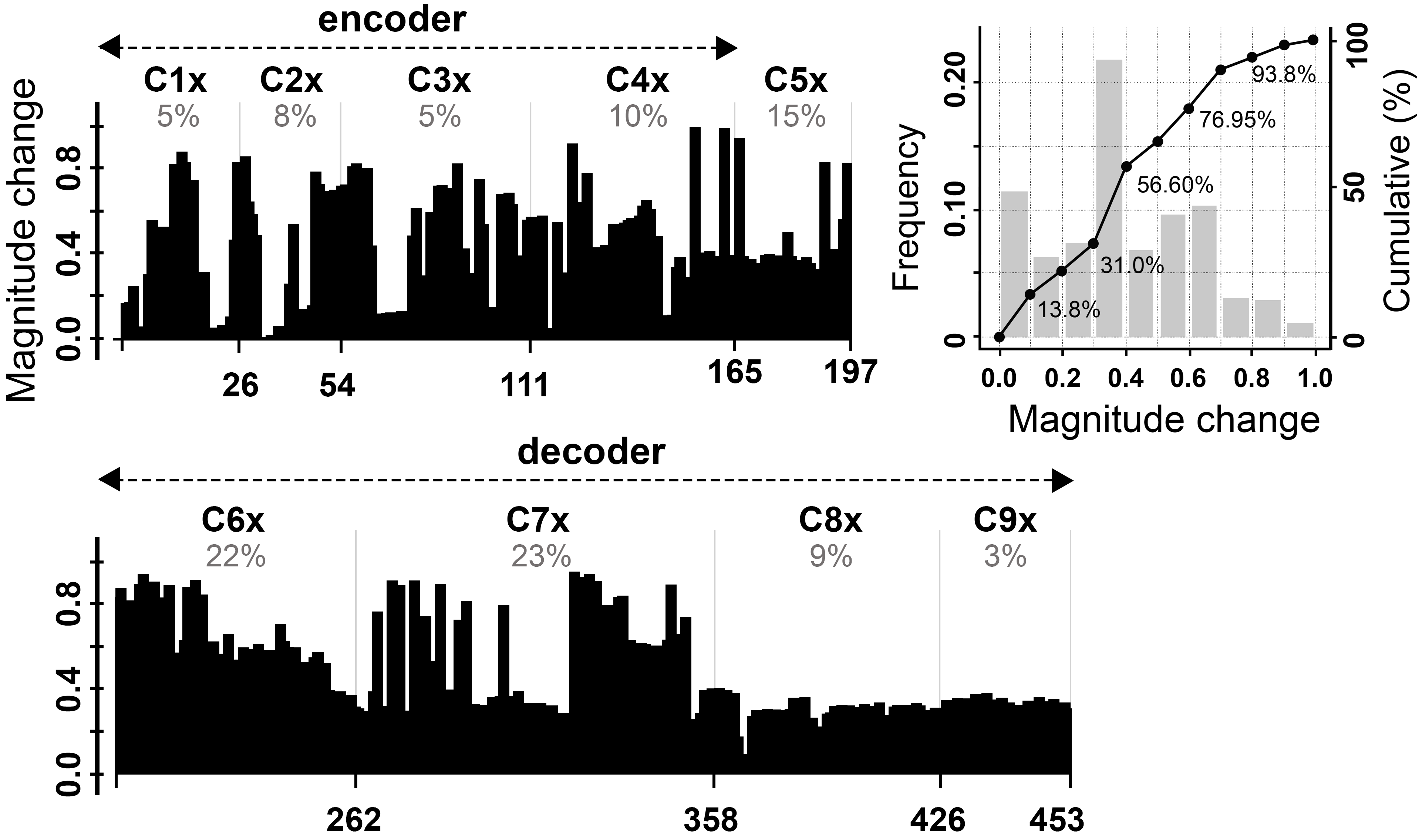
Figure 4: Normalized sum of mean activation changes calculated between 12 clusters, each having a minimum of 20 items. Percentage of total magnitude change is indicated per pairs of convolutional layers (e.g., C11 and C12 defined as C1x, see Table 1). Related distribution is shown in both, frequency and cumulative forms.

3.4. Similarity analysis

Preliminary results for similarity analysis help identifying data patterns among the 12,833 boots studied. Especially, queried objects appear to share characteristics with other similar instances in terms of colorimetry, texture and shape (Fig.5). However, this similarity decreases if such characteristics differ in the pool of analyzed objects i.e., the similarity score is less than 0.6 (see the last query example in Fig.5), or when investigating multiple queries jointly (Fig.6). Besides this, exploiting a large fraction of convolutional layers in similarity analysis seems important for satisfying results, given the speciation performance of these layers, as described in Section 3.3 and Fig.4. It should be noted that conducting the similarity analysis solely on individual parts of the network, such as the decoder or encoder alone, did not yield satisfactory results. Nonetheless, analogous results can still be achieved using features extracted from a ResNet50 model, trained to classify e.g., digits from the MNIST dataset (see Appendix B). This demonstrates the feasibility of applying the analytical approach for similarity computations described in this research to non-FCN models.

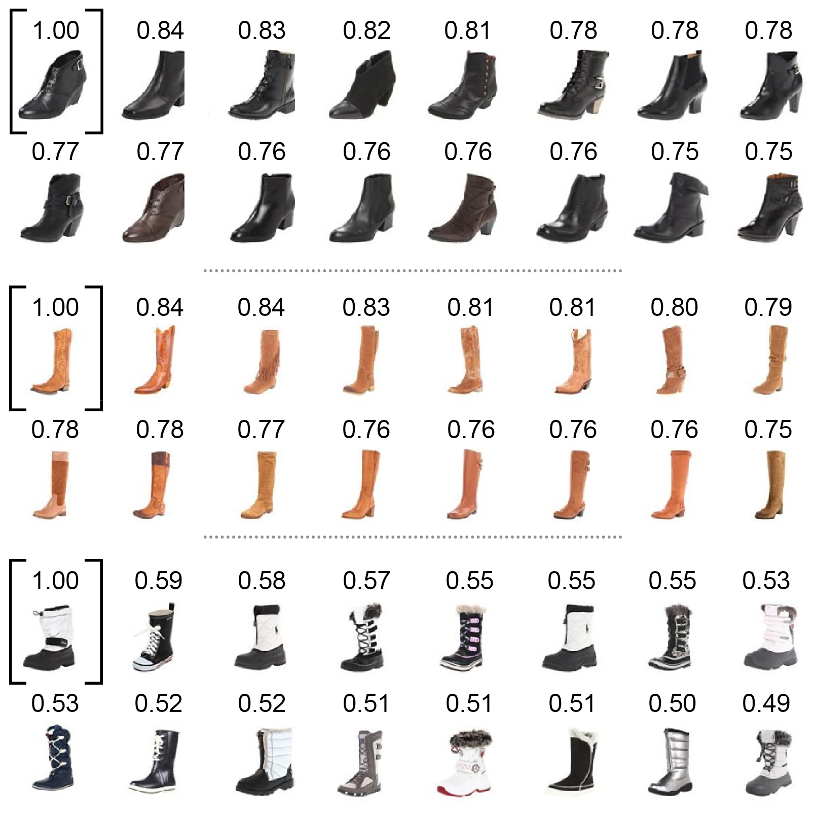
Figure 5: Examples of probabilistic similarity results for single queries (indicated by black square brackets) using a Gaussian membership function. Average values are indicated in decreasing order from top left to bottom right. Only 16 objects are shown per search.

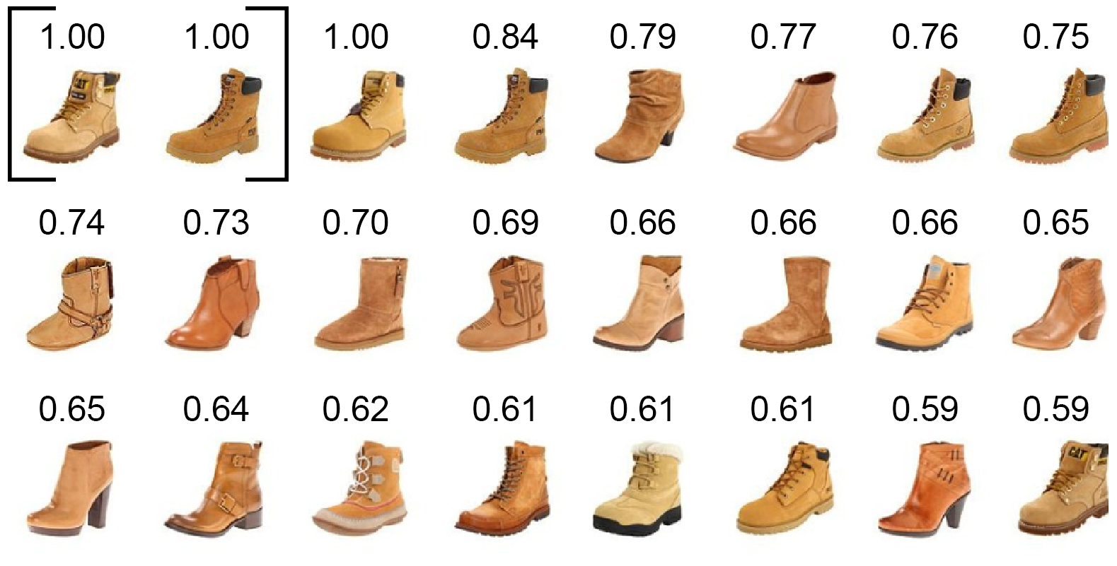
Figure 6: Example of probabilistic similarity results for two queries (indicated by black square brackets) using a trapezoidal membership function. Average values are presented in decreasing order from top left to bottom right. Only 24 objects shown.

4. Discussion

In this study, the distinctiveness of objects is objectively determined by the similarity algorithm and features of a trained network. It is more likely that object instances with consistent patterns i.e., well represented in data, end up having more similar objects with higher probabilistic values (closer to 1). Furthermore, the similarity search strategy is made possible with membership functions where subsets of activation magnitudes falling within the neighborhood of a query vector $v_{q}$ are grouped. Further studies may explore different search functions to construct fuzzy queries, such as triangular functions, without changing the properties of the method described in Section 2. More generally, it seems important to adapt similarity measures with the type of data analyzed. Notably, to the extent that subsets of activation patterns are evaluated by Gaussian functions, the shape of the search function is adjustable with a factor $\tau$, as defined in equation (2). Necessarily, a large $\tau$ implies to search for similar elements with lower memberships, which may be relevant for image datasets whose 2D objects have high variations in appearance.

The analysis of similar patterns in the UT Zappos50k dataset allows us to distinguish key recurring characteristics among different types of boots. These characteristics are embedded in the latent features of trained networks, and extracting them as fuzzy values helps determining valuable information from data. Qualitative evaluations of similar objects depicted in Fig. 5 and 6 offer interpretative insights, highlighting that certain boot details like colour, texture, and shape may carry more significance at the feature level, than minor characteristics like laces, buckles, and heels. Consequently, an object query does not inherently match perfectly other objects due to variations in elements such as laces, buckles, or heels. To achieve better matching, the extracted network information pertaining to these spatial elements should be assigned greater importance in the analysis. To do so, future practitioners may want to extract and evaluate latent features specific to certain object details, alongside with the main object's latent features. The work of [15] demonstrates this approach by dissecting both, the main object class, and its peculiar details as subclasses, giving extra importance to subclasses in similarity calculations by including latent information of each subclass in the analysis.

5. Conclusion

In this paper, a novel object-oriented similarity analysis method with fuzzy evidence of transformed network features facilitates the distinction of key patterns in data. The proposed approach demonstrates successful performance in image segmentation and effectively identifies object candidates based on attributes from one or multiple queries. The combination of transforming features from pre-trained models, fuzzy inference, and sparse learning allows for an intuitive determination of possible groups of similar 2D objects (surrogate classes) sharing analogous characteristics. This approach could be iteratively applied for clustering purposes, possibly by using a sequential partitioning of probabilistic similarity values. In addition, it can be envisioned to leverage the concept of fuzzy neighborhood in discretized feature space. Although sparse learning and pruning techniques are employed to reduce the dimensionality of $\mathcal{A}$, a significant portion of it serves as the foundation for similarity search. As such, it may be relevant to investigate alternative network architectures specifically tailored to the similarity scheme of this study to improve similarity results.

Appendix A: Sparse learning

Several studies utilize sparsification techniques to mitigate overparameterization and overfitting in neural networks. For further details, interested readers may refer to the comprehensive review by [20]. Sparsity often refers to the property of model parameters to contain numerous zero coefficients (sparsity of parameters), which may be exploited for computational and resource savings [21, 22, 23] or model simplification [24, 25]. When combined with pruning, sparse models can achieve high compression through sparse connectivity [26, 27, 28]. However, it is common to trade off accuracy for the reduction in model size and efficiency [29, 30]. In this study, the objective is not to compress networks or accelerate learning. Instead, the focus is on reducing the dimensionality of the activation space $\mathcal{A}$ during training, thereby pruning inactive (or unimportant) neural representations post-training for subsequent similarity evidence. Hence, the utilization of loss functions for both the main task and sparse learning aids in reducing active features during training on a selection of layers $\phi$. In this context, sparsity denotes the ratio of zeroed-out layer outputs at the channel level, which are pruned after completing the training process. Pruning is achieved via singular-value decomposition of a data matrix derived from $\mathcal{A}$ (see Section 2.1). It is important to note that the level of sparsity and pruning carries significant implications: (i) it simplifies and reduces the turnaround time of post-training feature extraction and examination using multivariate methods, (ii) it mitigates the high-dimensional characteristics of $\mathcal{A}$ (e.g., the curse of dimensionality), particularly when the number of network features studied from $\phi$ surpasses the number of observations (e.g., in the case of deep models trained on small datasets), and (iii) it promotes model generalization. Maximizing feature speciation in $\mathcal{A}$ is crucial, ensuring that non-pruned features are more likely to distinguish themselves through neural specialization, particularly in tasks like classification. Accordingly, some features are more relevant when studying activation magnitudes of $v_{i}$ for similarity analysis. This speciation is particularly of interest to induce heterogenous feature weighting (as formulated in Section 2.3).

To address sparse learning, penalties are applied using task- and sparse-related loss functions. Mathematical notations provided below are independent to notations used outside the Appendix A in this paper. Let $D$ be a dataset of $P$ input-output pairs ${\left\{\left(z_{i},y_{i}\right)\right\}\ }_{i=1}^{P}$, where $z_{i}$ is an input sample and $y_{i}$ the corresponding annotation. Assume $\Phi(\bullet;\theta)$ being the learning model parametrized by the weights $\theta$, which takes the input-output pairs of $D$ and optimizes $\theta$ given the cross-entropy loss $\mathcal{L(\bullet)}$. In the following, biases are omitted for notational simplicity. The task loss can be set by the formula

$$\mathcal{L}_{task}=\frac{1}{P}\left(\sum_{i=1}^{P}{\mathcal{L}\left(\Phi\left(z_{i};\theta\right),y_{i}\right)}\right).$$ (A1)

A convolutional layer $l$ transforms an input tensor $z^{l}\in\mathbb{R}^{H\times W\times C}$ into an output tensor $y^{l}\in\mathbb{R}^{H^{{}^{\prime}}\times W^{{}^{\prime}}\times K}$ using the filters $\theta^{l}\in\mathbb{R}^{K_{s}\times K_{s}\times C\times K}$, given $C$ inputs and $K$ output features. $H$ and $W$ represent respectively the height and width of inputs, while $K_{s}$ is the kernel size. Input tensors are individually convoluted with a set of 2D kernels $\left\{\theta_{j,k}^{l}\right\}_{k=1}^{C}$ such that the $j$th ouput $y_{j}^{l}$ is the sum of resulting convolutions ($\forall j\leq K$). The output is computed by the formula

$$y_{j}^{l}=\sum_{k=1}^{C}{\theta_{j,k}^{l}*z_{k}^{l}},\ \ s.t.\ \ y_{j}^{l}\in\mathbb{R}^{H^{{}^{\prime}}\times W^{{}^{\prime}}}.$$ (A2)

Let $u_{j}^{l}$ be the activated counterpart of $y_{j}^{l}$ using ReLU as the activation function. The channel-level ratio of non-zero (active) features $R_{sp}\in[0,1]$ is calculated for a selection of layers $\phi$ by converting $u_{j}^{l}$ into its respective scalar $r_{j}^{l}$:

$$R_{sp}=\frac{1}{|\phi|\times K}\sum_{l\in\phi}{\sum_{j=1}^{K}{sgn\left(r_{j}^{l}\right)}},$$ (A3)

where $\ r_{j}^{l}=\sum_{k,q}u_{j,k,q}^{l},\ \forall k\leq H^{{}^{\prime}},\ \forall q\leq W^{{}^{\prime}}$. The sign function $sgn(\bullet)$ converts $r_{j}^{l}$ to 1 if it is non-zero (positive), 0 otherwise. The opposite counterpart of $R_{sp}$ is the sparsity ratio $R_{sp}^{0}=1-R_{sp}$. To increase $R_{sp}^{0}$, negative values of $\theta^{l}$ are truncated to zero such that $\theta_{+}^{l}=max\left(0,\ \theta^{l}\right)$, and penalize the positive ones in $\theta_{+}^{l}$. To do so, $\theta_{+}^{l}$ is redefined as a $K$-dimensional vector $\xi^{l}$ by summing its elements from dimensions $K_{s}$ and $C$ over $K$. This vector is then summed with the $K$-dimensional bias vector of layer $l$ to constitute the vector $\xi^{l}=(e_{1,}^{l},\ldots,e_{K}^{l})$. The symbol $\xi$ denotes the resulting sum for notational convenience. The loss for channel-wise sparsity is given by

$$\mathcal{L}_{sp}=\frac{1}{|\phi|\times K}\sum_{l\in\phi}{\sum_{j=1}^{K}e_{j}^{l}}.$$ (A4)

Minimizing $\mathcal{L}_{sp}$ is trivial compared to the task loss $\mathcal{L}_{task}$, although reaching an objective $R_{sp}^{0}$ may sometimes require to re-scale $\mathcal{L}_{sp}$ in the final objective function. A weight factor $\lambda\in\mathbb{R}_{0}^{+}$ can be used for this purpose in the regularized objective function $\mathcal{R}$:

$$\begin{gathered}\begin{aligned} \mathcal{R}(\theta)&=\mathcal{L}_{\text{task}}+\lambda\mathcal{L}_{\text{sp}}\times\gamma,\\ \theta^{*}&=\underset{\theta}{\text{arg min}}\left\{\mathcal{R}(\theta)\right\},\end{aligned}\end{gathered}\quad\gamma=\left(\frac{R_{\text{sp}}-\beta}{1-\beta}\right)^{\alpha}.$$ (A5)

The term $\gamma$ limits sparse learning at a target non-zero features objective $\beta\in[0,1]$, given a learning speed defined by $\alpha$. The variables $\lambda$ and $\alpha$ are both evaluated experimentally.

Appendix B: Similarity analysis of digits from the MNIST dataset

A ResNet50 model is trained on the MNIST dataset with a sparsity level of 50%. This sparsity level is chosen to strike a balance between preserving essential features and reducing redundancy. Once the model is trained, similarity computations is conducted using the analytical procedure described in Section 2. In contrast to the conventional approach, where only a section of the feature map guided by segmentation outputs is used for magnitude calculations, the entire feature map generated by convolution is leveraged to compute the magnitude. This procedure allowed for precise and meaningful comparisons between various digit images within the dataset, without relying on segmentation results.

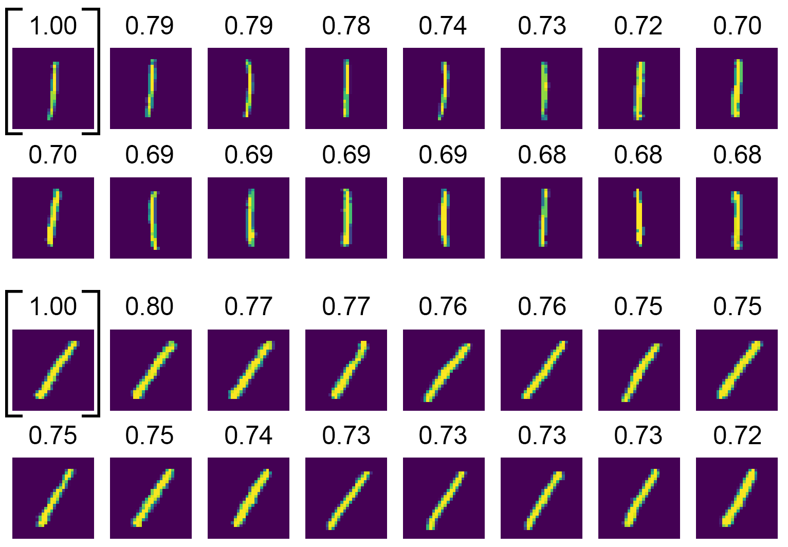
Figure B 1: Examples of similarity results for the queried digit “1”, using a Gaussian membership function and ResNet50 as feature extractor. Average values are presented in decreasing order, from top left to bottom right. Note the difference of digit orientation between the results of the two similarity queries.

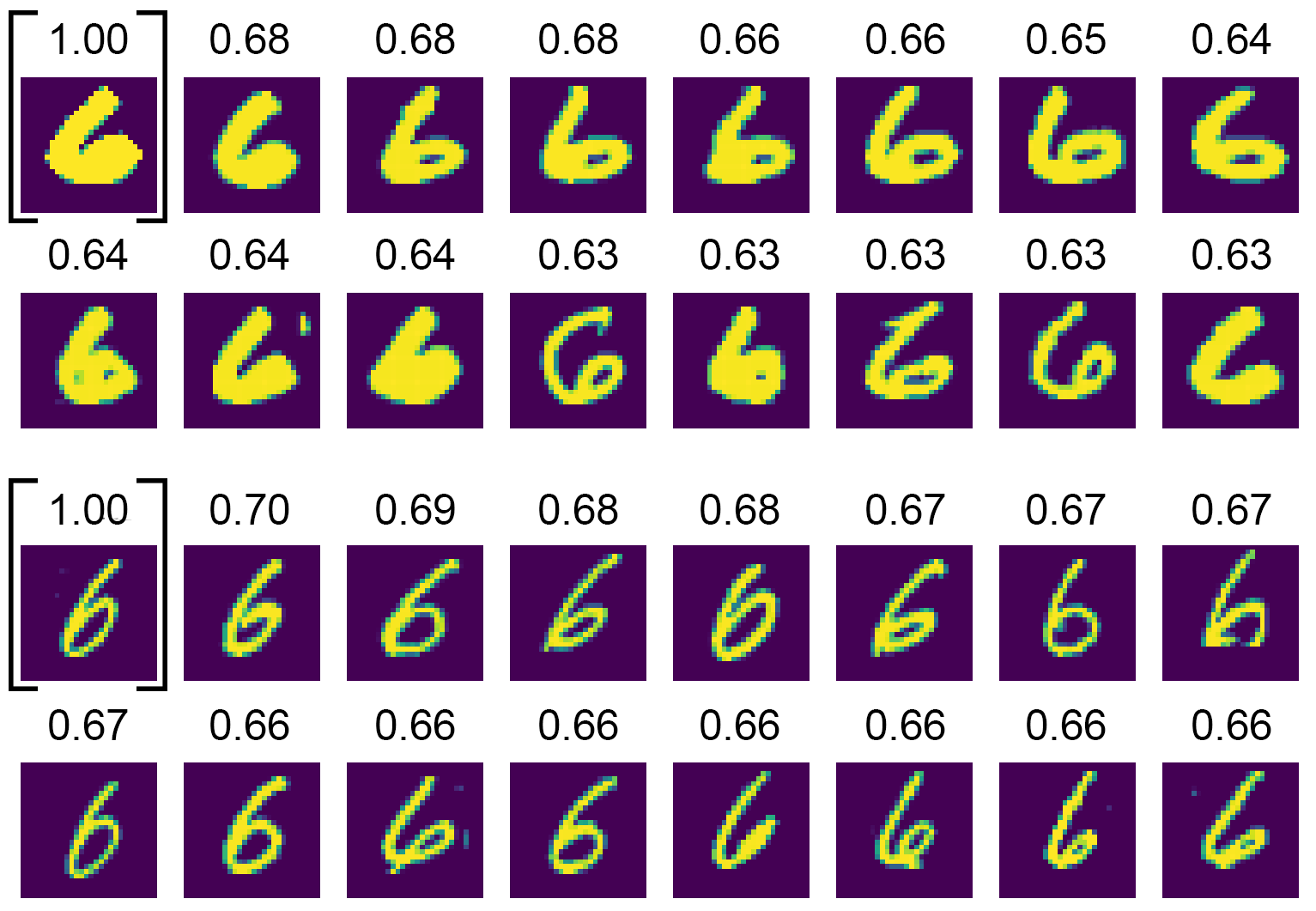
Figure B 2: Examples of similarity results for the queried digit “6”, using a Gaussian membership function and ResNet50 as feature extractor. Average values are presented in decreasing order, from top left to bottom right. Note the difference of line thickness between the results of the two similarity queries.

References

1. J. Wang, Y. Song, T. Leung, C. Rosenberg, J. Wang, J. Philbin, B. Chen and Y. Wu, “Learning fine-grained image similarity with deep ranking”, in Proceedings of the IEEE Conference on Computer Vision and Pattern Recognition, pp. 1386-1393, 2014.

2. S. Hanif, C. Li, A. Alazzawe and L. J. Latecki, “Image Retrieval with Similar Object Detection and Local Similarity to Detected Objects”, Pacific Rim Int. Conf. on Artificial Intelligence (PRICAI), Yanuca Island, Fiji, 2019.

3. Z. Ma, F. Liu, J. Dong, X. Qu, Y. He, S. Ji, “Hierarchical Similarity Learning for Language-based Product Image Retrieval”, in ICASSP 2021 - 2021 IEEE International Conference on Acoustics, Speech and Signal Processing (ICASSP), 2021.

4. S.-H. Cha, “Comprehensive Survey on Distance/Similarity Measures between Probability Density Functions”, International Journal of Mathematical Models and Methods in Applied Sciences, 1 (4) pp. 300-307, 2007.

5. C. Szegedy, W. Liu, Y. Jia, P. Sermanet, S. Reed, D. Anguelov, D. Erhan, V. Vanhoucke and A. Rabinovich, “Going deeper with convolutions”, in IEEE Conference on Computer Vision and Pattern Recognition (CVPR), Boston, MA, 1-9, 2015.

6. A. Krizhevsky, I. Sutskever and G.E. Hinton, “ImageNet Classification with Deep Convolutional Neural Networks”, Adv. Neural Inf. Process. Syst., 25, 2012.

7. G. Koch, R. Zemel, R. Salakhutdinov, “Siamese Neural Networks for One-shot Image Recognition”, in ICML deep learning workshop, vol. 2, 2015.

8. Y. Benajiba, J. Sun, Y. Zhang, L. Jiang, Z. Weng, O. Biran, “Siamese Networks for Semantic Pattern Similarity”, in IEEE 13th International Conference on Semantic Computing (ICSC), 2019.

9. L. Nanni, G. Minchio, S. Brahnam, G. Maguolo, A. Lumini, “Experiments of Image Classification Using Dissimilarity Spaces Built with Siamese Networks”, Sensor, 21(5), 1573, 2021.

10. A. Liao, M. Y. Yang, N. Zhan, B. Rosenhahn, “Triplet-based Deep Similarity Learning for Person Re-Identification” in IEEE International Conference on Computer Vision Workshops (ICCVW), 2017.

11. X. Yuan, Q. Liu, J. Long, L. Hu and Y. Wang, “Deep Image Similarity Measurement Based on the Improved Triplet Network with Spatial Pyramid Pooling”, Information, 10(4), 129, 2019.

12. K. Shall, K. U. Barthel, N. Hezel and K. Jung, “Deep Metric Learning using Similarities from Nonlinear Rank Approximation”, in IEEE 21st International Workshop on Multimedia Signal Processing (MMSP), 2019.

13. H. O. Song, Y. Xiang, S. Jegelka, S. Savarese, “Deep Metric Learning via Lifted Structured Feature Embedding”, in IEEE Conference on Computer Vision and Pattern Recognition (CVPR), 2016.

14. J. Long, E. Shelhamer, and T. Darrell, “Fully convolutional networks for semantic segmentation”, IEEE Conference on Computer Vision and Pattern Recognition (CVPR), 2015.

15. C. Juliani and E. Juliani, “Deep Learning of Terrain Morphology and Pattern Discovery via Network-based Representational Similarity Analysis for Deep-Sea Mineral Exploration”, Ore Geology Reviews, 129, 2020.

16. O. Ronneberger, P. Fischer, T. Brox, “U-Net: convolutional networks for biomedical image segmentation”, MICCAI 2015: Medical Image Computing and Computer-Assisted Intervention – MICCAI, pp: 234-241, 2015.

17. A. Yu and K. Grauman, "Fine-Grained Visual Comparisons with Local Learning", in CVPR '14: Proceedings of the 2014 IEEE Conference on Computer Vision and Pattern Recognition, pp. 192–199, 2014.

18. K. He, X. Zhang, S. Ren, J. Sun, “Deep Residual Learning for Image Recognition”, in IEEE Conference on Computer Vision and Pattern Recognition, 2016.

19. D.P. Kingma and J.L. Ba, “Adam: A method for stochastic optimization”, arXiv:1412.6980v9, 2015.

20. T. Gale, E. Elsen and S. Hooker, “The state of sparsity in deep neural networks”, arXiv:1902.09574v1, 2019.

21. B. Liu, M. Wang, H. Foroosh, M. Tappen and M. Penksy, “Sparse Convolutional Neural Networks”, in IEEE Conference on Computer Vision and Pattern Recognition (CVPR), 2015.

22. X. Xie, D. Du, Q. Li, Y. Liang, W.T. Tang, Z.L. Ong, M. Lu, H.P. Huynh and R.S.M. Goh, “Exploiting Sparsity to Accelerate Fully Connected Layers of CNN-Based Applications on Mobile SoCs”, ACM Trans. Embed. Comput. Syst.17, 2, Article 37, 2017.

23. P.A. Golnari and S. Malik, “Sparse matrix to matrix multiplication: A representation and architecture for acceleration”, arXiv:1906.00327v, 2019.

24. Z. Wang, F. Li, G. Shi, X. Xie and F. Wang, “Network pruning using sparse learning and genetic algorithm”, Neurocomputing, 404, 247-256, 2020.

25. Y. Li, S. Lin, B. Zhang, J. Liu, D. Doermann, Y. Wu, F. Huang and R. Ji, “Exploiting kernel sparsity and entropy for interpretable CNN compression”, arXiv:1812.04368, 2019.

26. S. Han, X. Liu, H. Mao, J. Pu, A. Pedram, M.A. Horowitz and W.J. Dally, “EIE: Efficient Inference Engine on Compressed Deep Neural Network”, arXiv:1602.01528”, 2016.

27. S. Han, H. Mao and W.J. Dally, “Deep compression: Compressing deep neural network with pruning, trained quantization and huffman coding”, arXiv:1510.00149, 2015.

28. W. Chen, J.T. Wilson, S. Tyree, K.Q. Weinberger and Y. Chen, “Compressing Neural Networks with the Hashing Trick”, arXiv:1504.04788, 2015.

29. M.H. Zhu and S. Gupta, “To prune, or not to prune: Exploring the efficacy of pruning for model compression”, arXiv:1710.01878v2, 2017.

30. B. Paria, C-K. Yeh, I.E.H. Yen, N. Xu, P. Ravikummar and B. Póczos, “Minimizing FLOPs to learn efficient sparse representations”, arXiv:2004.05665v1, 2020.