Calculating and resumming the classical virial expansion using automated algebra

Abstract

Using schematic model potentials, we calculate exactly the virial coefficients of a classical gas up to sixth order and use them to assess the convergence properties of the virial expansion of basic thermodynamic quantities such as pressure, density, and compressibility. At sufficiently strong couplings, as expected, the virial expansion fails to converge. However, at least for the interactions and parameter ranges we explored, we find that Padé-Borel resummation methods are extremely effective in improving the convergence of the expansion.

I Introduction

Understanding the finite-temperature thermodynamics of interacting matter represents an important and challenging problem across many areas of physics and chemistry. Notable applications are the dynamics of neutron star mergers (where the finite-temperature equations of state of neutron matter and nuclear matter play a central role), see e.g. [1, 2], and ultracold atomic gases [3, 4] (highly malleable systems created in many laboratories around the world). While both of those applications involve quantum matter, there are cases in chemistry and nuclear physics which are better suited for a classical description (usually at high-enough temperature that quantum effects are irrelevant or whenever those can be encoded into effective interactions), see e.g. [5]. Similarly, classical dynamics simulations of neutron matter at finite temperature have also been of interest [6]. This work focuses on such classical descriptions of many-particle systems at finite temperature.

At high temperatures and low densities, the virial expansion (VE) provides a rigorous approach to many-body equilibrium thermodynamics whereby each successive order $N$ adds on the contribution of the $N$-body problem to the grand-canonical description. Notably, in recent years the quantum VE has attracted considerable attention, in particular in connection with ultracold atomic gases [7, 8], but also as a way to characterize finite-temperature neutron star matter in dilute regimes (see e.g. [9, 10, 11]). Similarly, as explained in Ref. [5], there is also considerable activity in this direction in the area of chemistry, where the last decade has seen renewed interest in virial equations of state. In all of these cases, novel automated algebra approaches have enabled the calculation of high-order virial coefficients, allowing for the successful application of resummation techniques (see e.g. [12, 13]).

In this work, we focus on the application of the VE to a classical gas with a schematic interaction featuring a purely repulsive two-body force as well as a repulsive force with an attractive pocket at intermediate distances. Within the context of that interaction, we explore varying temperatures and coupling strengths in three spatial dimensions (although, as we explain below, our method is capable of calculating the VE in arbitrary dimensions). For this purpose, we have developed an automated algebra approach to the calculation of high-order VE coefficients (based on the seminal work of Ref. [14]), which is now available online at [15]. For the specific form of the schematic interaction considered here, our results for the coefficients of the VE are exact (up to numerical accuracy limitations) and therefore free of statistical effects (as no stochastic estimators are used in any way).

The remainder of this paper is organized as follows. Section II presents the formalism of the VE for a gas of identical particles, first in general form and then specializing to classical statistics. Section III explains the details of our approach to calculating the virial coefficients in an automated fashion. In Section IV, we show the schematic model interaction and corresponding results. Finally, in Section V, we summarize, conclude, and comment on the outlook of our work.

II Formalism

The VE organizes the many-body problem into a sum of $N$-body problems, specifically by Taylor-expanding the grand-canonical partition function ${\mathcal{Z}}$ in powers of the fugacity $z$, such that

$${\mathcal{Z}}=\sum_{N=0}^{\infty}Q_{N}z^{N},$$ (1)

where $Q_{N}$ is the $N$-particle canonical partition function, $z=e^{\beta\mu}$, $\beta$ is the inverse temperature, and $\mu$ is the chemical potential. The grand thermodynamic potential $\Omega$ is then given by

$$-\beta\Omega=\ln{\mathcal{Z}}=Q_{1}\sum_{N=1}^{\infty}b_{N}z^{N},$$ (2)

where $b_{N}$ are the virial coefficients

$$b_{1} = 1,$$ (3)

$$b_{2} = \frac{Q_{2}}{Q_{1}}-\frac{Q_{1}}{2!},$$ (4)

$$b_{3} = \frac{Q_{3}}{Q_{1}}-b_{2}Q_{1}-\frac{Q^{2}_{1}}{3!},$$ (5)

$$b_{4} = \frac{Q_{4}}{Q_{1}}-\left(b_{3}+\frac{b^{2}_{2}}{2}\right)Q_{1}-b_{2}\frac{Q^{2}_{1}}{2!}-\frac{Q^{3}_{1}}{4!},$$ (6)

and so on.

To make the connection to the quantum case more explicit, it is worth noting that in that case the expansion coefficients encode both quantum as well as interaction effects. Indeed, the coefficients of noninteracting quantum gases are generally non-vanishing, whereas their classical counterparts are all zero beyond $b_{1}$.

In the above expressions for $b_{N}$, the main contribution comes from the term $Q_{N}/Q_{1}$; the role of the remaining terms is to cancel out contributions from $Q_{N}$ that scale with super-linear powers of the spatial volume $V$. Once those cancellations are properly accounted for, the final result for $b_{N}$ is volume-independent. In practice, this property implies that one can focus exclusively on those terms in $Q_{N}$ that are proportional to $V$ [since $Q_{1}$ scales as $V$; see Eqs. (4)-(6)]. We use this property in our calculations, as further explained below.

For a classical gas of $N$ identical particles in $d$ spatial dimensions, the canonical partition function is

$$Q_{N}=\frac{1}{N!h^{dN}}\int d^{dN}{\bf p}\int d^{dN}{\bf r}\ e^{-\beta{\mathcal{H}}[\{\bf p\},\{\bf r\}]},$$ (7)

where

$${\mathcal{H}}[{\{\bf p\},\{\bf r\}}]=\sum_{i=1}^{N}\frac{{\bf p}_{i}^{2}}{2m}+\sum_{i<j}v_{ij}.$$ (8)

Here, ${\bf p}_{i}$ represents the momentum of the $i$-th particle, ${\bf r}_{i}$ its position, $m$ its mass (which will be assumed to be the same for all particles), and $v_{ij}=v(|{\bf r}_{i}-{\bf r}_{j}|)$ is the interaction potential energy that depends on the distance between particle $i$ and particle $j$. We focus in this work on pairwise interactions, but generalizations to three-body forces and beyond are possible. In contrast to the quantum case, where momentum and position operators do not commute (and one must resort to Trotter-Suzuki factorizations; see e.g. [16]), here the momenta can be integrated out, which yields

$$Q_{N}=\frac{1}{\lambda_{T}^{dN}N!}Z_{N},$$ (9)

where $\lambda_{T}=\sqrt{2\pi\hbar^{2}\beta/m}$ is the thermal wavelength and we define the configuration integral

$$Z_{N}=\int d^{dN}{\bf r}\exp\left({-\beta\sum_{i<j}v_{ij}}\right).$$ (10)

Capturing the interaction effects on the grand canonical partition function ${\mathcal{Z}}$ through the $b_{N}$’s amounts to calculating the interaction-induced change

$$\Delta Q_{N}=\frac{1}{\lambda_{T}^{dN}N!}\Delta Z_{N},$$ (11)

where

$$\Delta Z_{N}=\int d^{dN}{\bf r}\left[\exp\left({-\beta\sum_{i<j}v_{ij}}\right)-1\right].$$ (12)

In turn, the above $\Delta Q_{N}$ determine the change in the virial coefficients $\Delta b_{N}$, which enter into the thermodynamics via

$$-\beta\Delta\Omega=\ln({\mathcal{Z}}/{{\mathcal{Z}}}_{0})=Q_{1}\sum_{N=1}^{\infty}\Delta b_{N}z^{N},$$ (13)

where

$$\Delta b_{1} = 0,$$ (14)

$$\Delta b_{2} = \frac{\Delta Q_{2}}{Q_{1}},$$ (15)

$$\Delta b_{3} = \frac{\Delta Q_{3}}{Q_{1}}-\Delta b_{2}Q_{1},$$ (16)

and so forth, where we have used the fact that $\Delta Q_{1}=0$, since interactions only act among at least two particles.

The formalism presented above is the standard one due to Mayer [17] and often found in textbooks (see e.g. [18, 19]), albeit not always presented in as much detail as here. The above formulas apply to any two-body interaction. Below we show how our computational method organizes the calculation of $\Delta Z_{N}$ to access $\Delta b_{N}$.

III Computational method

III.1 Basic considerations

In order to calculate the central quantities $\Delta Z_{N}$, we use Mayer’s definition of the so-called $f$ function [17] given by

$$e^{-\beta v_{ij}}=1+f_{ij},$$ (17)

such that

$$\Delta Z_{N}=\int d^{dN}{\bf r}\left[\prod_{i<j}\left(1+f_{ij}\right)-1\right].$$ (18)

The product in this equation has $\binom{N}{2}$ factors and hence $2^{\binom{N}{2}}$ individual terms. One of these terms contains no $f$ functions (thus representing a noninteracting contribution) and is equal to unity, which will cancel out with the $-1$ term in the square bracket, thus leaving $2^{\binom{N}{2}}-1$ total terms in the integrand. Letting $n$ denote the number of $f$ functions that appear in a given term, each integrand is a product of the form $f_{i_{1}j_{1}}f_{i_{2}j_{2}}\cdots f_{i_{n}j_{n}}$, where $1\leq i_{k}<j_{k}\leq N$ and $1\leq n\leq\binom{N}{2}$.

Making the reasonable assumption that the interaction is translation-invariant, one may always factor out the center-of-mass motion, which upon integration shows that $\Delta Z_{N}$ scales at least as $V$. For the VE coefficients to remain finite, any terms scaling as a power of $V$ higher than linear must ultimately be cancelled out in the final expression for $\Delta b_{N}$ (otherwise the VE coefficients would be infinite in the thermodynamic limit) and can therefore be discarded right away. The computational job thus starts with selecting the terms in $\Delta Z_{N}$ that scale only linearly with $V$. To that end, note that any product of $f$ functions that does not contain all available indices $1,\dots,N$ will yield scaling with $V$ beyond linear and can therefore be discarded. Even if all the indices do appear in a given term, one must ensure that they do not form disjoint subsets, i.e. it must not be possible to factor the product of $f$’s into two (or more) sub-factors containing disjoint sets of indices. We comment more systematically on these properties below, after introducing a graph-based notation.

Following the definition used in [18], we establish a bijective correspondence between the integrals in Eq. (18) and undirected $N$-particle graphs. Let the nodes of an $N$-particle graph be labeled $1,2,\dots,N$. Given an arbitrary integral term, for each factor $f_{i_{k}j_{k}}$ appearing in the integrand (which has the form $f_{i_{1}j_{1}}f_{i_{2}j_{2}}\cdots f_{i_{n}j_{n}}$), connect an undirected edge between nodes $i_{k}$ and $j_{k}$. We then say that the graph represents the integral

$$\int d^{d}{\bf r}_{1}d^{d}{\bf r}_{2}\cdots d^{d}{\bf r}_{n}f_{i_{1}j_{1}}f_{i_{2}j_{2}}\cdots f_{i_{n}j_{n}}.$$ (19)

As examples, we show in Fig. 1 two contributions at order $N=5$, $n=5$ that scale as $V$ (and therefore contribute to the final result for $\Delta b_{5}$). Explicitly, they represent the integrals

$$\int d^{d}{\bf r}_{1}d^{d}{\bf r}_{2}d^{d}{\bf r}_{3}d^{d}{\bf r}_{4}d^{d}{\bf r}_{5}f_{12}f_{13}f_{14}f_{15}f_{23},$$ (20)

and

$$\int d^{d}{\bf r}_{1}d^{d}{\bf r}_{2}d^{d}{\bf r}_{3}d^{d}{\bf r}_{4}d^{d}{\bf r}_{5}f_{12}f_{13}f_{24}f_{45}f_{35},$$ (21)

respectively.

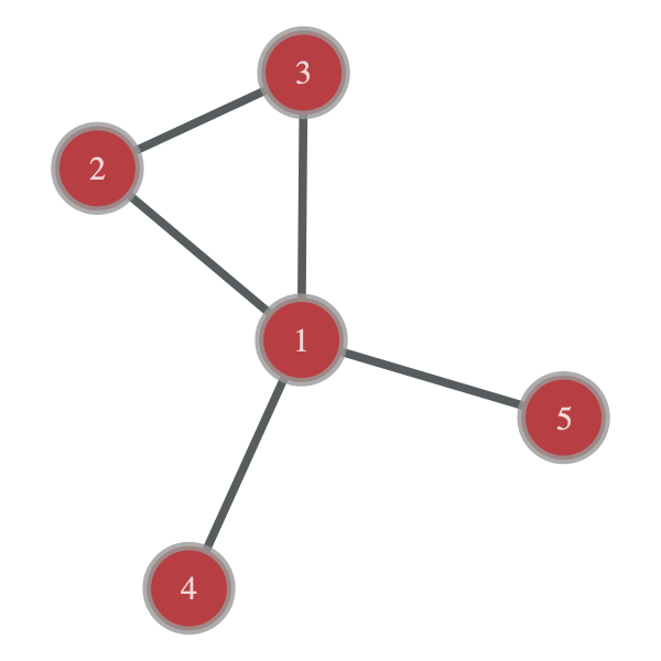
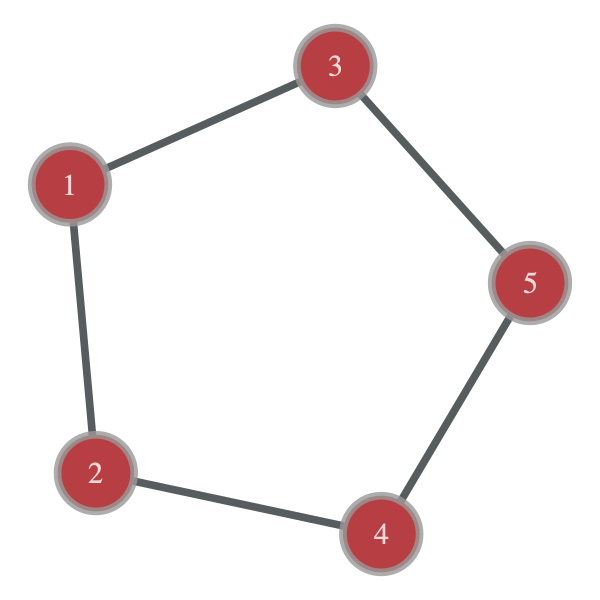
Figure 1: Two contributions at order $N=5$, $n=5$ that scale as $V$ and hence contribute to $\Delta b_{5}$.

As an example of a term that does not contribute to the final answer for $\Delta b_{5}$, we show in Fig. 2 a disconnected graph that represents the factorable integral

$$\int d^{d}{\bf r}_{1}d^{d}{\bf r}_{2}d^{d}{\bf r}_{3}f_{12}f_{23}f_{13}\int d^{d}{\bf r}_{4}d^{d}{\bf r}_{5}f_{45}.$$ (22)

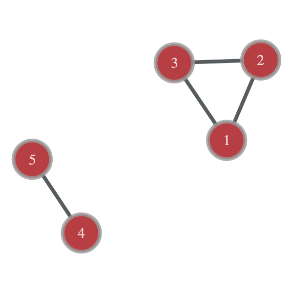
Figure 2: A contribution at order $N=5$, $n=4$ that scales as $V^{2}$, which cancels out in the final expression for $\Delta b_{5}$.

III.2 Systematic identification of contributing graphs

Since we are interested in the terms in $\Delta Z_{N}$ that scale as $V$, we start by considering all simple $N$-particle graphs with $n$ edges, $1\leq n\leq\binom{N}{2}$, corresponding to the $2^{\binom{N}{2}}-1$ terms in Eq. (18). The restriction to simple graphs excludes self-loops and multiple edges, for each factor $f_{ij}$ must have distinct indices and can appear at most once in a given integrand.

As explained above, any term will scale at least linearly in $V$ due to translational invariance, and any term that admits a disjoint factorization [e.g. Eq. (22)] will scale faster than $V$ and therefore not contribute to $\Delta b_{N}$. In the graphical representation, such factorability corresponds to a disconnected graph. Hence, any disconnected graph may be ignored. Since a graph must have at least $N-1$ nodes to be connected, this means that we can immediately discard all graphs with $n<N-1$ in our calculations. Next, assuming that all particles interact via the same pairwise potential, the result of each integral is invariant to permutation of the indices. Expressed graphically, this means that any two isomorphic graphs will yield the same numerical value upon computation. Graph isomorphism is an equivalence relation on a set of graphs, so we can partition the set of graphs with $n\geq N-1$ into isomorphism equivalence classes such that the integral terms in each are numerically equivalent.

At this point, we discard all graphs in equivalence classes representing disconnected diagrams (Discarding all graphs with $n<N-1$ was necessary but not sufficient for removing all disconnected graphs). We are thus left with a set of simply connected graphs partitioned into isomorphism classes. We can represent this collection with a “multiset”

$$\mathcal{G}^{*}=\{g_{1}G_{1},g_{2}G_{2},\dots\},$$ (23)

where the elements $G_{i}$ represent unique isomorphism class representatives and the repetition numbers $g_{i}$ represent the size of the corresponding isomorphism class. After numerically evaluating the $G_{i}$, we can form the vectors $\bm{g}=[g_{1}\ g_{2}\ \dots]^{T}$ and $\bm{G}=[G_{1}\ G_{2}\ \dots]^{T}$ and calculate Eq. (18) via

$$\Delta Z_{N}=\bm{g}^{T}\bm{G}.$$ (24)

Our implementation contains the combinatorial data of $\mathcal{G}^{*}$ (and hence can compute the VE coefficients) beyond the sixth order presented here. The data through order six were obtained by brute force isomorphism testing using the graph- tools library, which implements the VF2 algorithm of Cordella et al. (see [20]). The data for higher orders were obtained using the repository from Ref.[21] and the fact that

$$g_{i}=\frac{N!}{|\mathrm{Aut}(G_{i})|},$$ (25)

where $|\mathrm{Aut}(G_{i})|$ is the cardinality of the automorphism class of an $N$-particle graph $G_{i}$.

III.3 Integral evaluation

Evaluating Eq. (24) requires us to calculate each of the $dN$-dimensional integrals appearing in $\bm{G}$. A completely general treatment would involve constructing the functional form of each integrand and proceeding with a broadly applicable numerical integration method such as Newton-Cotes or Monte Carlo. We choose instead to base our scheme on the multivariate Gaussian identity

$$\int\exp(-\frac{1}{2}\bm{x}^{T}M\bm{x})d^{m}\bm{x}=\sqrt{\frac{(2\pi)^{m}}{\det M}},$$ (26)

where $M\in R^{m\times m}$ is a symmetric positive definite matrix and $x\in R^{m}$. While this identity corresponds to an exact integration only for potentials $v_{ij}$ that yield an integrand of this form when transformed through Eq. (17), the class of potentials for which this method is exact can emulate both a purely repulsive interaction and an interaction with an attractive pocket, as we describe below.

Additionally, this method is computationally efficient. The integrands never have to be constructed explicitly, and the results may be obtained by computing an $N\times N$ determinant, even though the integration space is $dN$-dimensional. Indeed, computing the VE coefficients to ninth order, which requires evaluating $\mathcal{O}(10^{5})$ unique integrals, can be accomplished in seconds. Lower orders can be achieved almost instantaneously, allowing one to plot smooth curves describing the evolution of the coefficients.

Another advantage of Eq. (26) is that it permits the use of non-integer dimensions. In our case, the dimension enters the result via $m=dN$ and the power to which we raise the eigenvalues of one block of the quadratic form represented by $A$. Thus, one could simply regard $d$ as a parameter of the investigation, such that examining how the VE coefficients change with dimension would amount to the exponentiation of scalars, sidestepping the already small cost of the determinant computations.

As a final note, our current implementation offers to approximate a general integrand with one of the form in Eq. (26). We have done this to provide some degree of generality to others who may use our code, but the general case is not the focus of this paper. We restrict our attention moving forward to those potentials for which the results are exact.

IV Model and Results

In this section we present our results for the pressure and density equations of state, as well as the isothermal compressibility. The approach detailed in the previous sections applies to an arbitrary two-body potential $v_{ij}$ where, in general, the integrals that result will not have exact analytic forms (i.e. one will not be able to use the simple result valid for Gaussians, mentioned above), such that a stochastic evaluation is needed, with the concomitant statistical uncertainties. To avoid such uncertainties, in this work we use a class of schematic model potentials for which an exact evaluation is possible. Specifically, we define our two-body interaction potential $v_{ij}$ to be such that

$$f_{ij}=Ae^{-b_{1}({\bf r}_{i}-{\bf r}_{j})^{2}}-(1+A)e^{-b_{2}({\bf r}_{i}-{\bf r}_{j})^{2}},$$ (27)

where $A,b_{1},b_{2}$ are constants; we will refer to this assumption as a Gaussian model. In other words, rather than fixing the shape of $v_{ij}$ and setting the inverse temperature $\beta$, and extracting $f_{ij}$ from them via Eq. (17), in this work we test our calculations by fixing the constants $A,b_{1},b_{2}$ above, thus letting the interaction to be dictated by

$$v_{ij}=-\frac{1}{\beta}\ln\left(1+f_{ij}\right).$$ (28)

In a realistic application, one would instead take $v_{ij}$ as an input and determine the temperature dependence of $A,b_{1},b_{2}$ by optimization.

With $f_{ij}$ given by Eq. (27), one may easily represent physically interesting situations such as a repulsive interaction (setting $A=0$ or $A=-1$), as well as a repulsive two-body potential with an attractive pocket (for $A>0$ or $A<-1$). In this work we explore both of those situations, shown schematically in Fig. 3.

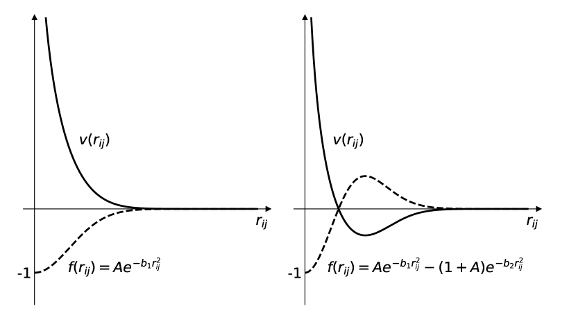
Figure 3: Left panel: Solid line shows the potential $v_{ij}$ as a function of $r_{ij}=|{\bf r_{i}}-{\bf r_{j}}|$, resulting from the Gaussian model of Eq. (27) setting $A=-1$, $b_{1}>0$, shown with a dashed line. Right panel: More general case corresponding to arbitrary $A>0$ and $b_{2}>b_{1}>0$ (or $A<-1$ and $b_{1}>b_{2}>0$).

IV.1 Purely repulsive interaction

In Fig. 4 we show our results for the virial coefficients $\Delta b_{N}$ of the purely repulsive Gaussian model (i.e. $A=-1$; see left panel of Fig. 3), as a function of the dimensionless coupling $\alpha=T/b_{1}$. As $\alpha$ grows, so do the interaction effects on the virial coefficients, as expected. In particular, we see how at large enough $\alpha$, high-order coefficients tend to become larger than their lower-order counterparts; this type of behavior was found as well in the quantum case in Refs. [12, 13] and it reflects the breakdown of the convergence properties of the series.

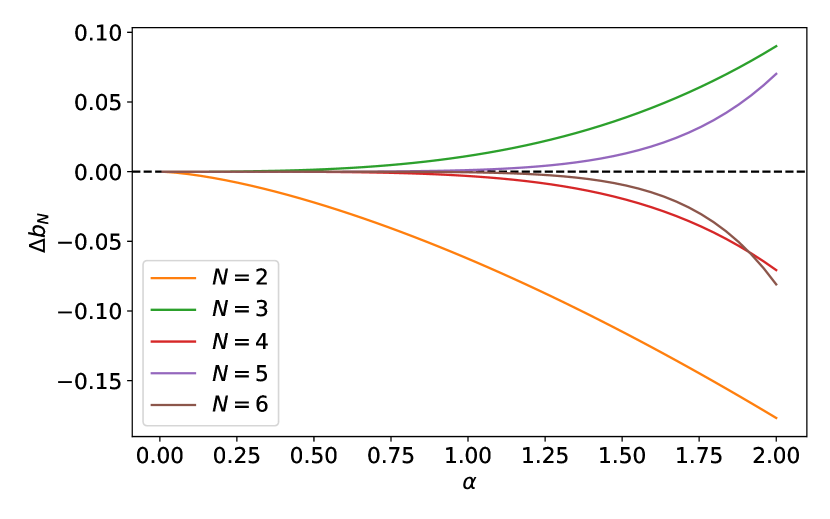
Figure 4: Virial coefficients $\Delta b_{N}$ for $N=2$,$3$,$4$,$5$,$6$ for the repulsive model ($A=-1$) as a function of the dimensionless coupling $\alpha=T/b_{1}$.

With the virial coefficients in hand, it is straightforward to evaluate the partial sums up to the available order for the pressure, density, and isothermal compressibility. They are given by

$$\frac{P}{P_{0}} = 1+\sum_{N=2}^{\infty}\Delta b_{N}z^{N-1},$$ (29)

$$\frac{n}{n_{0}} = 1+\sum_{N=2}^{\infty}N\Delta b_{N}z^{N-1},$$ (30)

and

$$\frac{\kappa}{\kappa_{0}}=\frac{1+\displaystyle\sum_{N=2}^{\infty}N^{2}\Delta b_{N}z^{N-1}}{\left(1+\displaystyle\sum_{N=2}^{\infty}N\Delta b_{N}z^{N-1}\right)^{2}},$$ (31)

where in all cases the subscript $0$ indicates the noninteracting case and we have used the thermodynamic identity

$$\kappa=\frac{\beta}{n^{2}}\left.\frac{\partial n}{\partial(\beta\mu)}\right|_{T}.$$ (32)

It is straightforward to evaluate Eqs. (29) and (30) as partial sums, but doing so for Eq. (32) requires a bit more care. As written, Eq. (32) will include partial contributions to higher orders, making it unclear what such an expression represents (e.g. Evaluating Eq. (32) with coefficients up to $\Delta b_{3}$ will not result in a quadratic plot, but will instead include the contributions of $\Delta b_{2}$ and $\Delta b_{3}$ to terms that are cubic and quartic in the fugacity). Hence, to keep Eq. (32) on the same footing as Eq. (29) and Eq. (30), we rewrite it as a single power series

$$\frac{\kappa}{\kappa_{0}}=\sum_{N=1}^{\infty}c_{N}z^{N-1},$$ (33)

where $c_{1}=1$ and

$$c_{2} = 0,$$ (34)

$$c_{3} = 3\Delta b_{3}-4\Delta b_{2}^{2},$$ (35)

$$c_{4} = 8\Delta b_{4}-24\Delta b_{2}\Delta b_{3}+16\Delta b_{2}^{3},$$ (36)

and so on. Eq. (33) truncated at $c_{N}$ then represents the largest partial sum of $\kappa/\kappa_{0}$ exactly computable using VE coefficients up to order $N$. [The analogous interpretation holds for Eqs. (29) and (30).]

Figures 5 through 8 show the above quantities for representative values of $\alpha$.

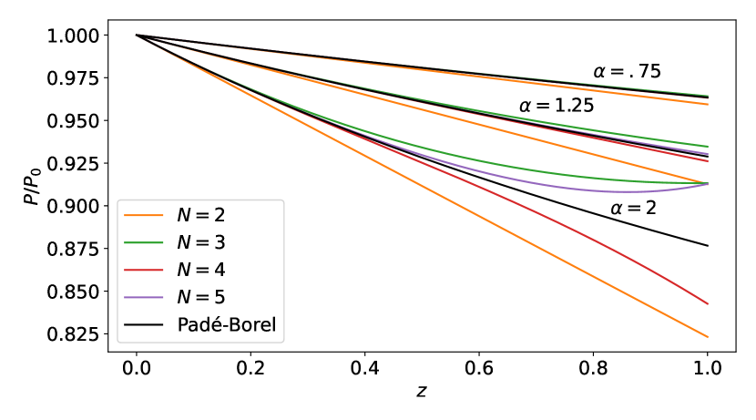
Figure 5: Pressure $P$ for the purely repulsive model, in units of its noninteracting counterpart $P_{0}$, as a function of the fugacity $z$ for three representative values of the dimensionless coupling $\alpha=T/b_{1}$. The colored lines show the highest value of the virial coefficient included, following the same convention as in Fig. 4. The black line shows the result of a Padé-Borel resummation, described below.

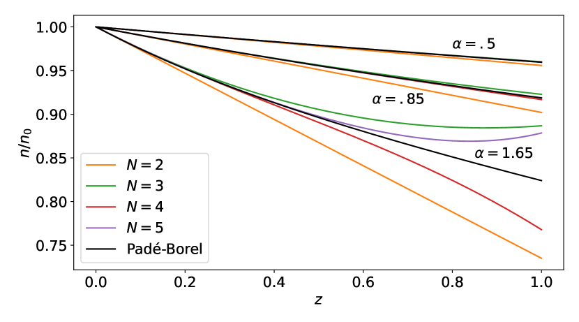
Figure 6: Density $n$ for the purely repulsive model, in units of its noninteracting counterpart $n_{0}$, as a function of the fugacity $z$ for three representative values of the dimensionless coupling $\alpha=T/b_{1}$. The colored lines show the highest value of the virial coefficient included, following the same convention as in Fig. 4. The black line shows the result of a Padé-Borel resummation, described below.

It is often useful to display the pressure-density equation of state, which amounts to a parametric plot that combines the information in Figs. 5 and 6. We show such a plot in Fig. 7.

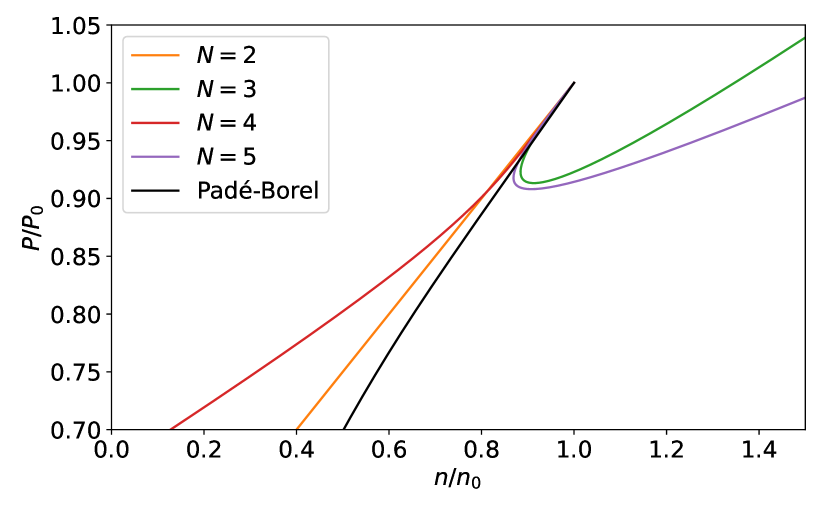
Figure 7: Pressure-density equation of state for the purely repulsive model at $\alpha=T/b_{1}=1.25$. The colored lines show the highest value of the virial coefficient included, following the same convention as in Fig. 4. The black line shows the result of a Padé-Borel resummation, described below.

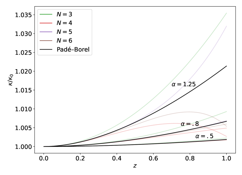
Figure 8: Compressibility $\kappa$ for the repulsive model, in units of its noninteracting counterpart $\kappa_{0}$, as a function of the fugacity $z$. The black line shows the result of a Padé-Borel resummation.

IV.1.1 Padé-Borel resummation of the VE

For strong enough interactions (in the sense of sufficiently large $\alpha$), the partial sums of the VE show clear signs of convergence failure. To address this issue, we resort to resummation methods, specifically Padé-Borel resummation. In this approach, one replaces a given power series (in our case the VE)

$$g(z)=\sum_{n=0}^{\infty}a_{n}z^{n},$$ (37)

with its Borel transform, namely

$$Bg(z)=\sum_{n=0}^{\infty}\frac{a_{n}}{n!}z^{n},$$ (38)

whose convergence properties can be expected to be more favorable than those of the partial sums of the original function $g(z)$. Using the highest available partial sum for $Bg(z)$, a Padé approximant is used as an ansatz to fit the resulting function. These approximants take the rational form $P(z)/Q(z)$, where $P$ and $Q$ are polynomials. Once a proper fit is obtained (in particular one that does not display poles for real values of $z$, which would be unphysical), the resummed function is obtained (in fact, defined within the context of the resummation method) via

$$g(z)=\int_{0}^{\infty}e^{-t}Bg(zt)dt,$$ (39)

which is evaluated numerically.

In each plot featuring a Padé-Borel resummation, the Padé approximant is fitted to the Borel transform of the highest partial sum displayed in the figure. Also, for all Padé approximants, $P(z)$ is linear and $Q(z)$ is quadratic. We experimented with different polynomials orders for $P$ and $Q$ but found that this combination behaved most reliably when performing the inverse transform of Eq. (39). The linear-quadratic approximant can replicate the Borel transforms of the pressure and density partial sums well, but the approximation quality lessens for the compressibility due to its increased curvature.

Figures 5 through 8 display the result of carrying out a Padé-Borel resummation on the series for the pressure, density, and compressibility. Our results show that this resummation approach vastly improves the convergence properties of the VE (at least for the quantities and parameter ranges studied).

IV.2 Repulsive interaction with attractive pocket

Encouraged by the results obtained for the purely repulsive interaction, we analyze here the more interesting case of an interaction that is repulsive at short distances but includes the more realistic feature of having an attractive pocket. We obtain the latter from Eq. (27) by setting $A=1$ (an arbitrary illustrative choice) and varying values of $\gamma=b_{2}/b_{1}$. At $\gamma=1$, the contribution from $A$ disappears in Eq. (27) and one recovers the repulsive case considered in the previous section. As $\gamma$ is increased beyond 1, an attractive pocket develops in the interaction (at a rate governed by the value of $A$), as shown qualitatively in Fig. 3 and Fig. 9.

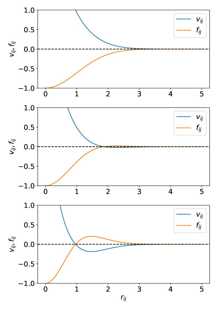
Figure 9: Potential $v_{ij}$ as a function of $r_{ij}=|{\bf r_{i}}-{\bf r_{j}}|$ (the horizontal axis is the same for all three plots), resulting from the Gaussian model of Eq. (27) setting $A=1$ and varying the value of $\gamma=b_{2}/b_{1}$. From top to bottom, the plots show the cases of $\gamma=1,1.4,$ and $2.5$, respectively.

In Fig. 10, we show the results of our calculations for the virial coefficients as a function of $\gamma$ at $\alpha=T/b_{1}=2$ (the latter being the strongest coupling considered in the previous section).

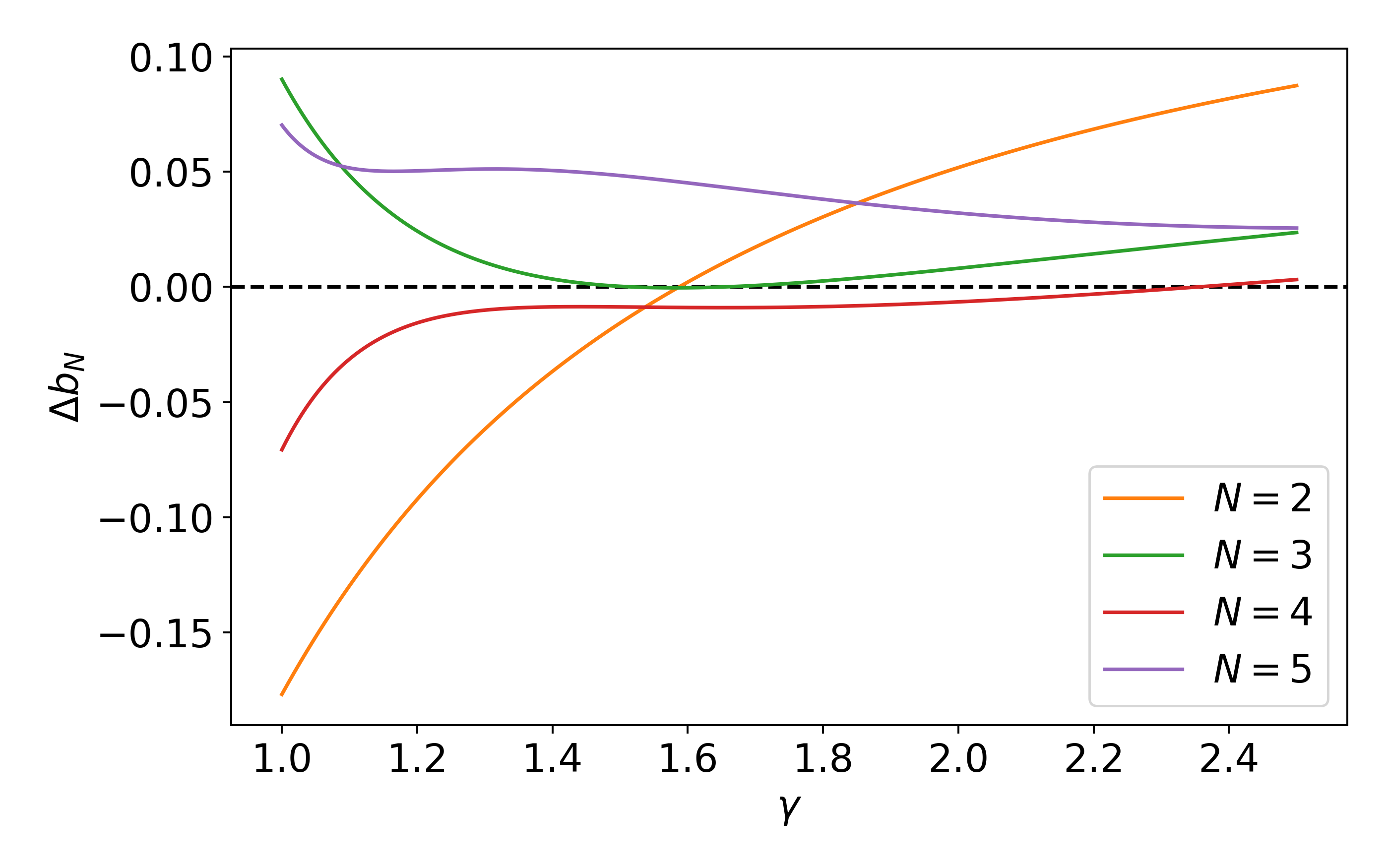
Figure 10: Virial coefficients $\Delta b_{N}$ for $N=2$, $3$, $4$, $5$ for the repulsive model with an attractive pocket ($A=1$, $\alpha=2$) as a function of the dimensionless coupling $\gamma=b_{2}/b_{1}$. At $\gamma=1$, the model becomes the purely repulsive limit of the previous section. As $\gamma$ is increased beyond 1, the attractive pocket develops, as shown in Fig. 9.

Following closely the discussion of the previous section, we show in Figs. 11 and 12 the pressure and compressibility, respectively, as functions of $z$, at fixed $\alpha$ and varying $\gamma\geq 1$, for the model with an attractive pocket. In each figure, the fixed value of $\alpha$ used is the strongest coupling considered in the corresponding purely repulsive case (see Figs. 5 and 8). Once again, our results show that this resummation approach vastly improves the convergence properties of the VE (at least for the quantities and parameter ranges studied).

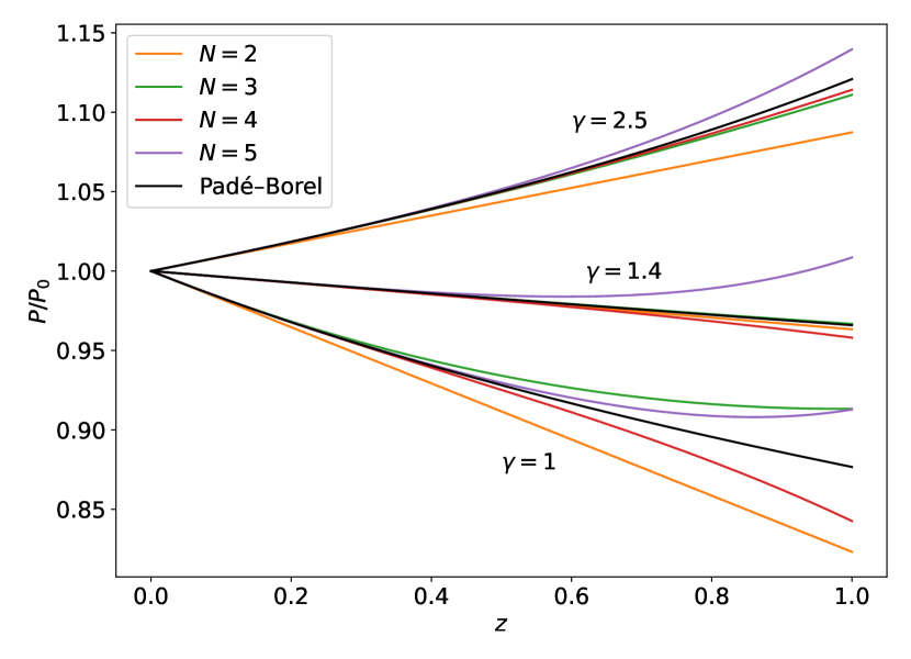
Figure 11: Pressure $P$ for the repulsive model with attractive pocket, in units of its noninteracting counterpart $P_{0}$, as a function of the fugacity $z$, for three different values of the interaction parameter $\gamma$. Note that $\gamma=1$ corresponds to the purely repulsive case studied in the previous section. The black line shows the result of a Padé-Borel resummation.

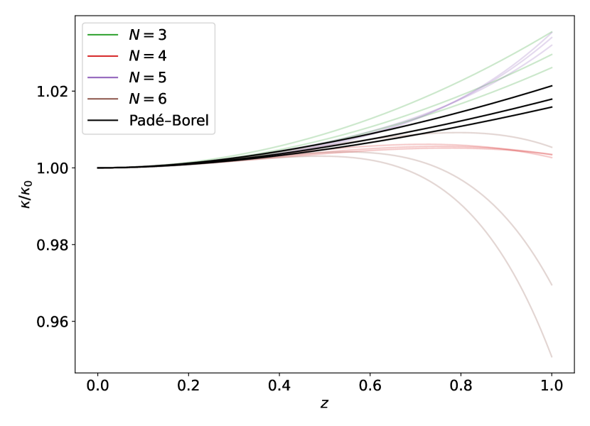
Figure 12: Compressibility $\kappa$ for the repulsive model with attractive pocket, in units of its noninteracting counterpart $\kappa_{0}$, as a function of the fugacity $z$. The black lines show the result of a Padé-Borel resummation, from top to bottom for $\gamma=1,1.03,1.05$, respectively.

V Conclusion and outlook

In this work we have explored, for a schematic model interaction encoding two different physical situations, the convergence properties of the VE of a classical gas. To that end, we have implemented an automated algebra approach to the calculation of high-order VE coefficients $\Delta b_{N}$. Using those, we calculated the pressure and density equations of state, as well as the isothermal compressibility.

As one of our main conclusions, we have found that resummation techniques such as Padé-Borel can vastly extend the applicability of the VE, at least for the class of models and parameter ranges we studied. Although we present this optimistic view, our results should be taken with the proverbial grain of salt, as the analytic properties of the VE are not well known for the specific family of models we considered.

Another main result of this work is the creation of an automated algebra package, which can be found online as the computational virial expansion engine (CVE²); see Ref. [14] and Ref. [15] for continued developments and releases. To the best of our knowledge, this is the first project addressing this problem by implementing an approach full based on automated algebra (without numerical integration), as presented here. Although we have only used CVE² to calculate up to $b_{6}$ in this work, the code is prepared to go beyond $b_{7}$ in its present form.

The most straightforward generalizations of our analysis, which will shed further light on the possibilities of the method, its implementation via CVE², and the properties of the VE, include extensions to multispecies systems (here we focused on identical particles of a single type), and within the latter the possibility of mass imbalance and spin polarization. Another aspect worth exploring is the dependence on spatial dimension, which is straightforward in our approach since the dimension enters analytically as a variable; in other words, within CVE², we can study classical gases not only in three spatial dimensions (as done here) and lower integer dimensions, but also in fractional dimensions, which may be of interest from the mathematical physics perspective.

Finally, it is worth pointing out that we explored here a schematic interaction where the Mayer factor $f$ was modeled as a single Gaussian function or a sum of two Gaussian functions. In future generalizations of this study, a higher number of Gaussians could be used to study, for instance, more realistic interactions such as screened Coulomb potentials. We leave such investigations to future work.