Template-Based Static Posterior Inference for Bayesian Probabilistic Programming

Abstract.

In Bayesian probabilistic programming, a central problem is to estimate the normalised posterior distribution (NPD) of a probabilistic program with score (a.k.a. observe) statements. Prominent approximate approaches to address this problem include Markov chain Monte Carlo (MCMC) and variational inference (VI), but neither of them is capable of generating guaranteed outcomes within a finite time limit. Moreover, most existing formal approaches that perform exact inference for NPD are restricted to programs with closed-form solutions to NPD or bounded loops/recursion. A recent work (Beutner et al., PLDI 2022) proposed an automated approach that derives guaranteed bounds for NPD over programs with unbounded recursion. However, as this approach requires recursion unrolling, it suffers from the path explosion problem. Furthermore, previous approaches do not consider score-recursive probabilistic programs that allow score statements inside loops, which is non-trivial and requires careful treatment to ensure the integrability of the normalising constant in NPD.

In this work, we propose a novel automated approach to derive bounds for NPD via polynomial templates, fixed-point theorems and Optional Stopping Theorem (OST). Our approach can handle probabilistic programs with unbounded while loops and continuous distributions with infinite supports. The novelties in our approach are three-fold: First, we use polynomial templates to circumvent the path explosion problem from recursion unrolling; Second, we derive a novel multiplicative variant of OST that addresses the integrability issue in score-recursive programs; Third, to increase the accuracy of the derived bounds via polynomial templates, we propose a novel technique of truncation that truncates a program into a bounded range of program values. Experiments over a wide range of benchmarks demonstrate that our approach is time-efficient and can derive bounds for NPD that are comparable with (or even tighter than) the recursion-unrolling approach (Beutner et al., PLDI 2022).

1. Introduction

In probabilistic programming, Bayesian statistical probabilistic programming adds specific statements for Bayesian reasoning into probabilistic programs. The principle of Bayesian probabilistic programming aims at first modelling probabilistic models as probabilistic programs and then analyzing the models through their program representation. Compared with traditional approaches (McIver and Morgan, 2004, 2005; Chakarov and Sankaranarayanan, 2013a; Chatterjee et al., 2016a) that specify an ad-hoc language, probabilistic programming languages (PPLs) (van de Meent et al., 2018) provide a universal framework to perform Bayesian inference. Unlike standard programming languages, PPLs have two specific constructs: sample and score (Borgström et al., 2016). The former construct allows drawing samples from a (prior) distribution, while the latter records the likelihood of observed data in the form of “score(weight)”. The universality of PPLs has the potential of enabling scientists and engineers to design and explore sophisticated probabilistic models easily: when using these languages, they no longer need to worry about developing custom inference engines for their models, which is previously a highly-nontrivial task that requires expertise in both statistics and machine learning. Thanks to its universality, Bayesian probabilistic programming has nowadays become an active research subject in both machine learning and programming language communities, and there have been an abundance of PPLs for Bayesian inference, such as Pyro(Bingham et al., 2019), WebPPL(Goodman and Stuhlmüller, 2014), Anglican(Tolpin et al., 2015), Church(Goodman et al., 2008), etc.

In this work, we consider the central problem of analyzing the normalised posterior distribution (NPD) in Bayesian inference over probabilistic programs. The general setting of this problem is that given a prior distribution $p(z)$ over the latent variables $z\in\mathbb{R}^{n}$ of interest and the distribution $p(x,z)$ of the probabilistic model represented by a probabilistic program, the task is to estimate the NPD by observing the evidence $x\in\mathbb{R}^{m}$ with the likelihood $p({x}{\mid}{z})$. Note that the problem can be generally solved by the Bayes’ rule $p({z}{\mid}{x})=\frac{p({x}{\mid}{z})p(z)}{p(x)}$, but the main difficulty to apply Bayes’ rule is that the normalising constant $p(x)=\int p({x}{\mid}{z})p(z)\mathrm{d}z$ is usually intractable to compute.

In the literature, there are two classes of approaches to address the NPD problem. The first is the approximate approaches that estimate the NPD by random simulations, while the second is the formal approaches that aim at deriving guaranteed bounds for NPD. In approximate approaches, two dominant methods are Markov chain Monte Carlo (MCMC) (Gamerman and Lopes, 2006) and variational inference (VI) (Blei et al., 2017). Although approximate approaches can produce approximate results efficiently, they cannot provide formal guarantee within a finite time limit. Moreover, as shown in  (Beutner et al., 2022), approximate approaches may produce inconsistent results between different simulation methods. In formal approaches, there is a large amount of previous works such as $(\lambda)$PSI (Gehr et al., 2016, 2020), AQUA (Huang et al., 2021), Hakaru (Narayanan et al., 2016) and SPPL (Saad et al., 2021), aiming to derive exact inference for NPD. However, these methods are restricted to specific kinds of programs, e.g., programs with closed-form solutions to NPD or without continuous distributions, and none of them can handle probabilistic programs with unbounded while-loops/recursion. Recently, Beutner et al. (Beutner et al., 2022) proposed an approach that infers guaranteed bounds for NPD and allows unbounded recursion. The main techniques in this approach are (i) the unrolling of every recursion in a probabilistic program to eliminate the appearance of recursion, (ii) the widening operator of abstract interpretation to eliminate the non-termination case in the unrolling and (iii) the interval semantics to handle continuous distributions.

Challenges and gaps.

In this work, we focus on developing formal approaches to derive bounds for NPD over probabilistic programs. In the previous formal approaches to address this problem, the most relevant work is Beutner et al. (2022), but it has the following drawbacks. The first is that this approach is based on recursion unrolling, and hence may cause path explosion. The second is that this approach cannot handle the situation where score statements with weight greater than $1$ appear inside a loop. In the sequel, we call such programs score-recursive, and show that score inside a loop may cause unbounded weights and integrability issues and thus requires careful treatment. Staton et al. (Staton et al., 2016) also noted that for a non-recursive $\lambda$-calculus with score, unbounded weights may introduce the possibility of “infinite model evidence errors”. To circumvent the second drawback, previous results (e.g., Borgström et al. (Borgström et al., 2016)) allow only $1$-bounded weights, and no existing approaches can handle score-recursive programs whose weight of score can be greater than $1$.

Template-based approaches.

To avoid the path explosion problem arising from the recursion unrolling method (Beutner et al., 2022), we consider the template paradigm (Chakarov and Sankaranarayanan, 2013b; Chatterjee et al., 2018, 2016a) that first sets up a numerical template for the bound function to be solved, then establishes constraints for the template which is derived from the underlying verification theory (e.g. fixed point theory, Optional Stopping Theorem, etc.), and finally solves the template based on the derived constraints to obtain a concrete bound function. Template-based approaches have been shown to be capable of synthesizing tight bounds for expectation and probabilistic properties over probabilistic programs (Wang et al., 2019, 2021b), and are time efficient since they can leverage highly optimized constraint solvers for linear, semidefinite, and convex programming, etc. Therefore, the template paradigm serves as a good candidate to address the NPD problem in Bayesian probabilistic programming. However, simply applying the template paradigm does not suffice by the following reasons:

• The most accurate numerical template by far is polynomial template. However, polynomial template is tight only over a bounded region (see e.g. Weierstrass Approximation Theorem (Jeffreys, 1988)), and in general is not accurate over an unbounded region.

• The common pattern for a template-based approach is to synthesize a single bound function via a single process of template solving. However, having a single template is not enough for synthesizing tight bounds for NPD, as different initial program inputs may need different bound functions to achieve tight bounds.

In this work, we have careful treatment to address the two weakness above. Our detailed contributions are as follows.

Our contributions.

In this work, we present the following contributions:

• First, to circumvent the path explosion from loop unrolling (that corresponds to recursion unrolling in functional programs) in the previous work (Beutner et al., 2022), we propose a novel approach that uses polynomial templates (Chatterjee et al., 2016b, 2020; Wang et al., 2019), fixed-point theorems (Tarski, 1955) and Optional Stopping Theorem (OST) (Williams, 1991) to synthesize polynomial bounds for NPD.

• Second, to address the integrability issue from score-recursive programs, we present a novel multiplicative variant of the classical OST to derive expectation bounds. This addresses the challenge of handling score-recursive probabilistic programs stated previously.

• Third, to increase the accuracy of the derived bounds, we propose a novel truncation operation that truncates the probabilistic program of concern onto a bounded range of program values, which allows our algorithm to explore high-degree polynomials to improve the accuracy of the derived bounds. Moreover, we devise our algorithm in the way to synthesize multiple bounds for various initial program inputs to further improve the accuracy. The truncation operation and the synthesis of multiple bounds address the weakness of the existing template-based approaches in the literature.

• Finally, experimental results show that our approach can handle a wide range of benchmarks including non-parametric examples such as Pedestrian (Beutner et al., 2022) and score-recursive examples such as phylogenetics (Ronquist et al., 2021). Compared with the previous approach (Beutner et al., 2022), our approach reduces the runtime by up to $6$ times, while deriving comparable or even tighter bounds for NPD.

Technical contributions.

Compared with the previous results on the use of template paradigm and OST, we propose a truncation operation (onto a bounded range of program values) that leverages the approximability of polynomials over a bounded region, and a multiplicative variant of OST that can handle score-recursive programs.

Limitations.

One limitation is that our approach has the combinatorial explosion that when the degree of the polynomial template increases, the time of the template solving increases exponentially. However, from our experimental results, a moderate choice of the degree (e.g., no more than $10$) suffices. Another is that for sampling statements with continuous distributions, our approach currently assumes polynomial density functions. However, with proper approximation via (piecewise) polynomials, our approach can handle any continuous density functions.

2. Preliminaries

We first review some basic concepts from probability theory (see standard textbooks such as (Pollard, 2002; Williams, 1991) for a detailed treatment), and then present the Bayesian probabilistic programming language and the normalised posterior distribution (NPD) problem. Throughout the paper, we denote by $\mathbb{N}$, $\mathbb{Z}$ and $\mathbb{R}$ the sets of all natural numbers (including zero), integers, and real numbers, respectively.

2.1. Basics of Probability Theory

A measurable space is a pair $(U,\Sigma_{U})$, where $U$ is a nonempty set and $\Sigma_{U}$ is a $\sigma$-algebra on $U$, i.e., a family of subsets of $U$ such that $\Sigma_{U}\subseteq\mathcal{P}(U)$ contains $\emptyset$ and is closed under complementation and countable union. Elements of $\Sigma_{U}$ are called measurable sets. A function $f$ from a measurable space $(U_{1},\Sigma_{U_{1}})$ to another measurable space $(U_{2},\Sigma_{U_{2}})$ is measurable if $f^{-1}(A)\in\Sigma_{U_{1}}$ for all $A\in\Sigma_{U_{2}}$.

A measure $\mu$ on a measurable space $(U,\Sigma_{U})$ is a mapping from $\Sigma_{U}$ to $[0,\infty]$ such that (i) $\mu(\emptyset)=0$ and (ii) $\mu$ is countably additive: for every pairwise-disjoint set sequence $\{A_{n}\}_{n\in\mathbb{N}}$ in $\Sigma_{U}$, it holds that $\mu(\bigcup_{n\in\mathbb{N}}A_{n})=\sum_{n\in\mathbb{N}}\mu(A_{n})$. We call the triple $(U,\Sigma_{U},\mu)$ a measure space. If $\mu(U)=1$, we call $\mu$ a probability measure, and $(U,\Sigma_{U},\mu)$ a probability space. The Lebesgue measure $\lambda$ is the unique measure on $(\mathbb{R},\Sigma_{\mathbb{R}})$ satisfying $\lambda([a,b))=b-a$ for all valid intervals $[a,b)$ in $\Sigma_{\mathbb{R}}$. For each $n\in\mathbb{N}$, we have a measurable space $(\mathbb{R}^{n},\Sigma_{\mathbb{R}^{n}})$ and a unique product measure $\lambda_{n}$ on $\mathbb{R}^{n}$ satisfying $\lambda_{n}(\prod_{i=1}^{n}A_{i})=\prod_{i=1}^{n}\lambda(A_{i})$ for all $A_{i}\in\Sigma_{\mathbb{R}}$.

The Lebesgue integral operator $\int$ is a partial operator that maps a measure $\mu$ on $(U,\Sigma_{U})$ and a real-valued function $f$ on the same space $(U,\Sigma_{U})$ to a real number or infinity, which is denoted by $\int f\mathrm{d}\mu$ or $\int f(x)\mu(\mathrm{d}x)$. The detailed definition of Lebesgue integral is somewhat technical, see (Rankin, 1968; Rudin et al., 1976) for more details. Given a measurable set $A\in\Sigma_{U}$, the integral of $f$ over $A$ is defined by $\int_{A}f(x)\mu(\mathrm{d}x):=\int f(x)\cdot[x\in A]\mu(\mathrm{d}x)$ where $[-]$ is the Iverson bracket such that $[\phi]=1$ if $\phi$ is true, and $0$ otherwise. If $\mu$ is a probability measure, then we call the integral as the expectation of $f$, denoted by $\mathbb{E}_{x\sim\mu;A}\left[{f}\right]$, or $\mathbb{E}[f]$ when the scope is clear from the context.

For a measure $v$ on $(U,\Sigma_{U})$, a measurable function $f:U\to\mathbb{R}_{\geq 0}$ is the density of $v$ with respect to $\mu$ if $v(A)=\int f(x)\cdot[x\in A]\mu(\mathrm{d}x)$ for all measurable $A\in\Sigma_{U}$, and $\mu$ is called the reference measure (most often $\mu$ is the Lebesgue measure). Common families of probability distributions on the reals, e.g., uniform, normal distributions, are measures on $(\mathbb{R},\Sigma_{\mathbb{R}})$. Most often these are defined in terms of probability density functions with respect to the Lebesgue measure. That is, for each $\mu_{D}$ there is a measurable function $\text{pdf}_{D}:\mathbb{R}\to\mathbb{R}_{\geq 0}$ that determines it: $\mu_{D}(A):=\int_{A}\text{pdf}_{D}(\mathrm{d}\lambda)$. As we will see, density functions such as $\text{pdf}_{D}$ play an important role in Bayesian inference.

Given a probability space $(\Omega,\mathcal{F},\mathbb{P})$, a random variable is an $\mathcal{F}$-measurable function $X:\Omega\rightarrow\mathbb{R}\cup\{+\infty,-\infty\}$. The expectation of a random variable $X$, denoted by $\mathbb{E}(X)$, is the Lebesgue integral of $X$ w.r.t. $\mathbb{P}$, i.e., $\int X\,\mathrm{d}\mathbb{P}$. A filtration of $(\Omega,\mathcal{F},\mathbb{P})$ is an infinite sequence $\{\mathcal{F}_{n}\}_{n=0}^{\infty}$ such that for every $n\geq 0$, the triple $(\Omega,\mathcal{F}_{n},\mathbb{P})$ is a probability space and $\mathcal{F}_{n}\subseteq\mathcal{F}_{n+1}\subseteq\mathcal{F}$. A stopping time w.r.t. $\{\mathcal{F}_{n}\}_{n=0}^{\infty}$ is a random variable $T:\Omega\rightarrow\mathbb{N}\cup\{0,\infty\}$ such that for every $n\geq 0$, the event {$T\leq n$} is in $\mathcal{F}_{n}$.

A discrete-time stochastic process is a sequence $\Gamma=\{X_{n}\}_{n=0}^{\infty}$ of random variables in $(\Omega,\mathcal{F},\mathbb{P})$. The process $\Gamma$ is adapted to a filtration $\{\mathcal{F}_{n}\}_{n=0}^{\infty}$, if for all $n\geq 0$, $X_{n}$ is a random variable in $(\Omega,\mathcal{F}_{n},\mathbb{P})$. A discrete-time stochastic process $\Gamma=\{X_{n}\}_{n=0}^{\infty}$ adapted to a filtration $\{\mathcal{F}_{n}\}_{n=0}^{\infty}$ is a martingale (resp. supermartingale, submartingale) if for all $n\geq 0$, $\mathbb{E}(|X_{n}|)<\infty$ and it holds almost surely (i.e., with probability $1$) that ${\mathbb{E}}{\left[{X_{n+1}}\mid{\mathcal{F}_{n}}\right]}=X_{n}$ (resp. ${\mathbb{E}}{\left[{X_{n+1}}\mid{\mathcal{F}_{n}}\right]}\leq X_{n}$, ${\mathbb{E}}{\left[{X_{n+1}}\mid{\mathcal{F}_{n}}\right]}\geq X_{n}$). See (Williams, 1991) for details. Applying martingales to qualitative and quantitative analysis of probabilistic programs is a well-studied technique (Chakarov and Sankaranarayanan, 2013a; Chatterjee et al., 2016a, 2017).

2.2. Bayesian Probabilistic Programming Language

The syntax of our probabilistic programming language (PPL) is given in Fig. 1, where the metavariables $S$, $B$ and $E$ stand for statements, boolean expressions and arithmetic expressions, respectively. Our PPL is imperative with the usual conditional and loop structures (i.e., if and while), as well as the following new structures: (a) sample constructs of the form “$\textbf{sample}\ D$” that sample a value from a prescribed distribution $D$ over $\mathbb{R}$ and then assign this value to a sampling variable $r$; (b) score statements of the form “score($EW$)” that weight the current execution with a value expressed by $EW$ (note that $\textit{pdf}(D,x)$ means the value of a probability density function w.r.t. $D$ at $x$); (c) probabilistic branching statements of the form “$\textbf{if}\ \textbf{prob}(p)\dots$” that lead to the then part with probability $p\in(0,1]$ and to the else part with probability $1-p$. We also have sequential compositions (i.e., ";") and support return statements (i.e., return) that return the value of the program variable of interest. Note that $c,c_{1},c_{2}\in\mathbb{R}$ are constants, and our language supports any distributions with continuous density functions and infinite supports, including but not limited to uniform and normal distributions.

$$S ::=\textbf{skip}\mid x:=ES\mid\textbf{score}(EW)\mid\textbf{return}\ x\mid S_{1};S_{2}$$

$$\mid\mbox{{while}}\,B\,\text{{do}}\,S\,\text{{od}}\mid\mbox{{if}}\,\mbox{$B$}\,\mbox{{then}}\,S_{1}\,\mbox{{else}}\,S_{2}\,\mbox{{fi}}\mid\mbox{{if}}\,\mbox{{prob}($p$)}\,\mbox{{then}}\,S_{1}\,\mbox{{else}}\,S_{2}\,\mbox{{fi}}$$

$$B ::=\textbf{true}\mid\textbf{false}\mid\neg B\mid B_{1}\,\textbf{and}\,B_{2}\mid B_{1}\,\textbf{or}\,B_{2}\mid E_{1}\leq E_{2}\mid E_{1}\geq E_{2}$$

$$E ::=x\mid c\mid E_{1}+E_{2}\mid E_{1}-E_{2}\mid E_{1}*E_{2}\ \ \ ES::=E\mid\textbf{sample}\ D$$

$$EW ::=E\mid\textit{pdf}(D,x)\ \ \ D::=\textbf{normal}(c_{1},c_{2})\mid\textbf{uniform}(c_{1},c_{2})\mid\cdots$$

Figure 1. Syntax of Our Probabilistic Programming Language

Given a probabilistic program in our language, we distinguish two disjoint sets of variables in the program: (i) the set $V_{\mathrm{p}}$ of program variables whose values are determined by assignments in the program (i.e., the expressions at the LHS of “:="); (ii) the set $V_{\mathrm{r}}$ of sampling variables whose values are independently sampled from prescribed probability distributions each time they are accessed (i.e., each “$\textbf{sample}\ D$" can be regarded as a sampling variable $r$).

Example 2.1.

Fig. 3 shows a Bayesian probabilistic program written in our PPL language. In this program, the set of program variables is $V_{\mathrm{p}}=\{start,pos,dis,step\}$, and the set of sampling variables is $V_{\mathrm{r}}=\{\textbf{sample uniform}(0,1)\}$. Each time $\textbf{sample uniform}(0,1)$ is executed, it samples a value uniformly from $[0,1]$ and then assigns the value to the variable $step$. ∎

⬇

$\mbox{\sl start}:=$ sample uniform$(0,3)$;

$\mbox{\sl pos}:=\mbox{\sl start}$; $\mbox{\sl dist}:=0$;

$\ell_{\mathrm{init}}:$ while $\mbox{\sl pos}\geq 0$ do

$\mbox{\sl step}:=$ sample uniform$(0,1)$;

if prob($0.5$) then

$\mbox{\sl pos}:=\mbox{\sl pos}-\mbox{\sl step}$

else

$\mbox{\sl pos}:=\mbox{\sl pos}+\mbox{\sl step}$

fi;

$\mbox{\sl dist}:=\mbox{\sl dist}+\mbox{\sl step}$

od;

score(normal($1.1$,$0.1$),dist);

return start

$\ell_{\mathrm{out}}:$

Figure 2. A Pedestrian Random Walk

Figure 3. The WPTS of Pedestrian

2.3. The Semantics of Our Programming Language

Let $V$ be a finite set of variables with an implicit linear order over its elements. A valuation on $V$ is a function $\mathbf{v}:V\rightarrow\mathbb{R}$ that assigns a real value to each variable in $V$. We denote the set of all valuations on $V$ by $\mbox{\sl Val}_{V}$. For each $1\leq i\leq|V|$, we denote the value of the $i$-th variable (in the implicit linear order) in $\mathbf{v}$ by $\mathbf{v}[i]$, so that we can view each valuation as a real vector on $V$. A program (resp. sampling) valuation is a valuation on $V_{\mathrm{p}}$ (resp. $V_{\mathrm{r}}$), respectively. For the sake of convenience, we fix the notations in the following way, i.e., we always use $\mathbf{v}\in\mbox{\sl Val}_{V_{\mathrm{p}}}$ to denote a program valuation, and $\mathbf{r}\in\mbox{\sl Val}_{V_{\mathrm{r}}}$ to denote a sampling valuation; we also write $\mathbf{v}[\mathit{ret}]$ for the value of the return variable in $\mathbf{v}$.

Below we present the semantics for our programming language. Existing semantics in the literature are either measure-(Staton et al., 2016; Lee et al., 2020) or sampling-based (Mak et al., 2021; Beutner et al., 2022). To facilitate the development of our algorithm, we consider the transition-based semantics (Chakarov and Sankaranarayanan, 2013b; Chatterjee et al., 2016b) to our language and treat each probabilistic program as a weighted probabilistic transition system (WPTS). A WPTS extends a PTS  (Chakarov and Sankaranarayanan, 2013b; Chatterjee et al., 2016b) with weights and an initial probability distribution.

Definition 2.2 (WPTS).

A weighted probabilistic transition system (WPTS) $\Pi$ is a tuple

(†) $$\Pi=(V_{\mathrm{p}},V_{\mathrm{r}},L,\ell_{\mathrm{init}},\ell_{\mathrm{out}},\mu_{\mathrm{init}},\mathcal{D},\mathfrak{T})$$

for which:

• $V_{\mathrm{p}}$ and $V_{\mathrm{r}}$ are finite disjoint sets of program and resp. sampling variables.

• $\mathit{L}$ is a finite set of locations with special locations $\ell_{\mathrm{init}},\ell_{\mathrm{out}}\in\mathit{L}$. Informally, $\ell_{\mathrm{init}}$ is the initial location and $\ell_{\mathrm{out}}$ represents program termination.

• $\mu_{\mathrm{init}}$ is the initial probability distribution over $\mathbb{R}^{V_{\mathrm{p}}}$ with a finite support (denoted by $\textsf{supp}\left({\mu_{\mathrm{init}}}\right)$), while $\mathcal{D}$ is a function that assigns a probability distribution $\mathcal{D}(r)$ to each $r\in V_{\mathrm{r}}$. We call each $\mathbf{v}\in\textsf{supp}\left({\mu_{\mathrm{init}}}\right)$ an initial program valuation, and abuse the notation so that $\mathcal{D}$ also denotes the independent joint distribution of all $\mathcal{D}(r)$’s ($r\in V_{\mathrm{r}}$).

• $\mathfrak{T}$ is a finite set of transitions where each transition $\tau\in\mathfrak{T}$ is a tuple $\langle\ell,\phi,F_{1},\dots,F_{k}\rangle$ such that (i) $\ell\in L$ is the source location of the transition, (ii) $\phi$ is the guard condition which is a predicate over variables $V_{\mathrm{p}}$, and (iii) each $F_{j}:=\langle\ell^{\prime}_{j},p_{j},\mbox{\sl upd}_{j},\mbox{\sl wt}_{j}\rangle$ is called a weighted fork for which (a) $\ell^{\prime}_{j}\in L$ is the destination location of the fork, (b) $p_{j}\in(0,1]$ is the probability of this fork, (c) $\mbox{\sl upd}_{j}:\mathbb{R}^{|V_{\mathrm{p}}|}\times\mathbb{R}^{|V_{\mathrm{r}}|}\rightarrow\mathbb{R}^{|V_{\mathrm{p}}|}$ is an update function that takes as inputs the current program and sampling valuations and returns an updated program valuation in the next step, and (d) $\mbox{\sl wt}_{j}:\mathbb{R}^{|V_{\mathrm{p}}|}\times\mathbb{R}^{|V_{\mathrm{r}}|}\to[0,\infty)$ is a score function that gives the likelihood weight of this fork depending on the current program and sampling valuations.

In a WPTS, we use update and score functions to model the update on the program variables and resp. the likelihood weight when running a basic block of statements in a program, respectively. If there is no score statement in the block, then the score function is constantly $1$. We always assume that a WPTS $\Pi$ is deterministic and total, i.e., (i) there is no program valuation that simultaneously satisfies the guard conditions of two distinct transitions from the same source location, and (ii) the disjunction of the guard conditions of all the transitions from any source location is a tautology. The transformation from a probabilistic program into its WPTS can be done in a straightforward way (see e.g. (Chatterjee et al., 2018; Chakarov and Sankaranarayanan, 2013b)).

Example 2.3.

Fig. 3 shows the WPTS of the program in Fig. 3 which has two locations $\ell_{\mathrm{init}},\ell_{\mathrm{out}}$. The circle nodes represent locations and square nodes model the forking behavior of transitions. An edge entering a square node is labeled with the condition of its respective transition, while an edge entering a circle node stands for a fork, which is associated with its probability, update functions and score functions that marked by $w$. The value of $step$ is initialised to $0$. An the initial probability distribution $\mu_{\mathrm{init}}$ is determined by the joint distribution of $(start,pos,dis,step)$ where $start\sim uniform(0,3)$ and $pos,dis,step$ observe the Dirac measures $Dirac(\{start\})$, $Dirac(\{0\})$ and $Dirac(\{0\})$, respectively, e.g., the probability of the event “$dis\in\{0\}$” equals $1$. As $step$ simply receives values from a sampling variable, we neglect it in the WPTS.∎

We say that a WPTS is non-score-recursive if for all transitions $\tau=\langle\ell,\phi,F_{1},F_{2},\dots,F_{k}\rangle$ in the WPTS with each fork $F_{j}=\langle\ell^{\prime}_{j},p_{j},\mbox{\sl upd}_{j},\mbox{\sl wt}_{j}\rangle$ ($1\leq j\leq k$), we have that each score function $\mbox{\sl wt}_{j}$ is constantly $1$ (i.e., the multiplicative weight does not change) for every $\ell^{\prime}_{j}\neq\ell_{\mathrm{out}}$. Otherwise, the WPTS is score-recursive. Informally, a non-score-recursive WPTS has non-trivial score functions only on the transitions to the termination of a program, while a score-recursive WPTS has score statements in the execution of the program. For example, the WPTS of the program in Section 3.1 is non-score-recursive as the nontrivial (i.e., score values not equal to $1$) score statement only appears to the termination, while the WPTS of the program in Section 3.2 is score recursive since it has score statements inside the loop body. In the case of a non-score-recursive WPTS, we say that the WPTS is score-bounded by a positive real $M>0$ if for every $\tau=\langle\ell,\phi,F_{1},F_{2},\dots,F_{k}\rangle$ in the WPTS with $F_{j}=\langle\ell^{\prime}_{j},p_{j},\mbox{\sl upd}_{j},\mbox{\sl wt}_{j}\rangle$ ($1\leq j\leq k$), we have that $|\mbox{\sl wt}_{j}|\leq M$ whenever $\ell^{\prime}_{j}=\ell_{\mathrm{out}}$.

Given a program valuation $\mathbf{v}$ and a predicate $\phi$ over variables $V_{\mathrm{p}}$, we say that $\mathbf{v}$ satisfies $\phi$ (written as $\mathbf{v}\models\phi$) if $\phi$ holds when the variables in $\phi$ are substituted by their values in $\mathbf{v}$. A state is a pair $\Xi=(\ell,\mathbf{v})$ where $\ell\in L$ (resp. $\mathbf{v}\in\mathbb{R}^{|V_{\mathrm{p}}|}$) represents the current location (resp. program valuation), respectively, while a weighted state is a triple $\Theta=(\ell,\mathbf{v},w)$ where $(\ell,\mathbf{v})$ is a state and $w\in[0,\infty)$ represents the multiplicative likelihood weight accumulated so far.

Below we specify the semantics of a WPTS. Consider a WPTS $\Pi$ in the form of († ‣ 2.2). The semantics of $\Pi$ is formalized by the infinite sequence $\Gamma=\{\widehat{\Theta}_{n}=(\widehat{\ell}_{n},\widehat{\mathbf{v}}_{n},\widehat{w}_{n})\}_{n\geq 0}$ where each $(\widehat{\ell}_{n},\widehat{\mathbf{v}}_{n},\widehat{w}_{n})$ is the random weighted state at the $n$th execution step of the WPTS such that $\widehat{\ell}_{n}$ (resp. $\widehat{\mathbf{v}}_{n}$, $\widehat{w}_{n}$) is the random variable for the location (resp. the random vector for the program valuation, the random variable for the multiplicative likelihood weight) at the $n$th step, respectively. The sequence $\Gamma$ starts with the initial random weighted state $\widehat{\Theta}_{0}=(\widehat{\ell}_{0},\widehat{\mathbf{v}}_{0},\widehat{w}_{0})$ such that $\widehat{\ell}_{0}$ is constantly $\ell_{\mathrm{init}}$, $\widehat{\mathbf{v}}_{0}\in\textsf{supp}\left({\mu_{\mathrm{init}}}\right)$ is sampled from the initial distribution $\mu_{\mathrm{init}}$ and the initial weight $\widehat{w}_{0}$ is constantly set to $1$. Then, given the current random weighted state $\widehat{\Theta}_{n}=(\widehat{\ell}_{n},\widehat{\mathbf{v}}_{n},\widehat{w}_{n})$ at the $n$th step, the next random weighted state $\widehat{\Theta}_{n+1}=(\widehat{\ell}_{n+1},\widehat{\mathbf{v}}_{n+1},\widehat{w}_{n+1})$ is determined by: (a) If $\widehat{\ell}_{n}=\ell_{\mathrm{out}}$, then $(\widehat{\ell}_{n+1},\widehat{\mathbf{v}}_{n+1},\widehat{w}_{n+1})$ takes the same weighted state as $(\widehat{\ell}_{n},\widehat{\mathbf{v}}_{n},\widehat{w}_{n})$ (i.e., the next weighted state stays at the termination location $\ell_{\mathrm{out}}$); (b) Otherwise, $\widehat{\Theta}_{n+1}$ is determined by the following procedure:

• First, since the WPTS $\Pi$ is deterministic and total, we take the unique transition $\tau=\langle\hat{\ell}_{n},\phi,F_{1},\dots,F_{k}\rangle$ such that $\hat{\mathbf{v}}_{n}\models\phi$.

• Second, we choose a fork $F_{j}=\langle\ell_{j},p_{j},\mbox{\sl upd}_{j},\mbox{\sl wt}_{j}\rangle$ with probability $p_{j}$.

• Third, we obtain a sampling valuation $\mathbf{r}\in\textsf{supp}\left({\mathcal{D}}\right)$ by sampling each $r\in V_{\mathrm{r}}$ independently w.r.t the probability distribution $\mathcal{D}(r).$

• Finally, the value of the next random weighted state $(\widehat{\ell}_{n+1},\widehat{\mathbf{v}}_{n+1},\widehat{w}_{n+1})$ is determined as that of $(\ell^{\prime}_{j},\mbox{\sl upd}_{j}(\hat{\mathbf{v}}_{n},\mathbf{r}),\widehat{w}_{n}\cdot\mbox{\sl wt}_{j}(\widehat{\mathbf{v}}_{n},\mathbf{r}))$.

Given the semantics, a program run of the WPTS $\Pi$ is a concrete instance of $\Gamma$, i.e., an infinite sequence $\omega=\{\Theta_{n}\}_{n\geq 0}$ of weighted states where each $\Theta_{n}=(\ell_{n},\mathbf{v}_{n},w_{n})$ is the concrete weighted state at the $n$th step in this program run with location $\ell_{n}$, program valuation $\mathbf{v}_{n}$ and multiplicative likelihood weight $w_{n}$. A state $(\ell,\mathbf{v})$ is called reachable if there exists a program run $\omega=\{\Theta_{n}\}_{n\geq 0}$ such that $\Theta_{n}=(\ell,\mathbf{v},w_{n})$ for some $n$.

Example 2.4.

Consider the WPTS in Example 2.3. Consider an initial program valuation $(1,1,0)$ which means that the initial values of $start,pos,dis$ are $1,1,0$, respectively. Then starting from the initial weighted state $(\ell_{\mathrm{init}},(1,1,0),1)$, a program run w.r.t the WPTS semantics above could be

$$(\ell_{\mathrm{init}},(1,1,0),1)\to(\ell_{\mathrm{init}},(1,0.5,0.5),1)\to(\ell_{\mathrm{init}},(1,-0.1,1.1),1)\to(\ell_{\mathrm{out}},(1,-0.1,1.1),3.9894).\qed$$

Given an initial program valuation $\mathbf{v}_{\mathrm{init}}$ of a WPTS, one could construct a probability space over the program runs by their probabilistic evolution described above and standard constructions such as general state space Markov chains (Meyn and Tweedie, 2012). We denote the probability measure in the probability space by $\mathbb{P}_{\mathbf{v}_{\mathrm{init}}}(-)$ and the expectation operator by $\mathbb{E}_{\mathbf{v}_{\mathrm{init}}}\left[{-}\right]$.

2.4. Normalised Posterior Distribution

Before presenting the central problem of Bayesian probabilistic programming, i.e., analyzing normalised posterior distribution with our WPTS models, we introduce some technical concepts.

Definition 2.5 (Termination).

The termination time of a WPTS $\Pi$ is the random variable $T$ given by $T(\omega):=\text{min}\{n\in\mathbb{N}\mid\ell_{n}=\ell_{\mathrm{out}}\}$ for every program run $\omega=\{(\ell_{n},\mathbf{v}_{n},w_{n})\}_{n\geq 0}$ where $\text{min}\,\emptyset:=\infty$. That is, $T(\omega)$ is the number of steps a program run $\omega$ takes to reach the termination location $\ell_{\mathrm{out}}$. A WPTS $\Pi$ is almost-surely terminating (AST) if $\mathbb{P}_{\mathbf{v}_{\mathrm{init}}}(T<\infty)=1$ for all initial program valuations $\mathbf{v}_{\mathrm{init}}\in\textsf{supp}\left({\mu_{\mathrm{init}}}\right)$.

Definition 2.6 (Expected Weights).

Given a WPTS $\Pi$ in the form of († ‣ 2.2), a designated initial program valuation $\mathbf{v}_{\mathrm{init}}$ and a measurable subset $\mathcal{U}\in\Sigma_{\mathbb{R}^{|V_{\mathrm{p}}|}}$, the expected weight $\llbracket\Pi\rrbracket_{\mathbf{v}_{\mathrm{init}}}(\mathcal{U})$ is defined as $\llbracket\Pi\rrbracket_{\mathbf{v}_{\mathrm{init}}}(\mathcal{U}):=\mathbb{E}_{\mathbf{v}_{\mathrm{init}}}\left[{[\widehat{\mathbf{v}}_{T}\in\mathcal{U}]\cdot\widehat{w}_{T}}\right]$.

By definition, we have that $\widehat{\mathbf{v}}_{T}$ (resp. $\widehat{w}_{T}$) is the random vector (resp. variable) of the program valuation (resp. the multiplicative likelihood weight) at termination, respectively. Thus, $\llbracket\Pi\rrbracket_{\mathbf{v}_{\mathrm{init}}}(\mathcal{U})$ is the expectation of $\widehat{w}_{T}$ that start from the state $(\ell_{\mathrm{init}},\mathbf{v}_{\mathrm{init}},1)$ and end with $\widehat{\mathbf{v}}_{T}\in\mathcal{U}$. If $\mathcal{U}=\mathbb{R}^{|V_{\mathrm{p}}|}$, the restriction of $\widehat{\mathbf{v}}_{T}\in\mathcal{U}$ can be removed.

Below we define the normalised posterior distribution (NPD) problem.

Definition 2.7 (Normalised Posterior Distribution).

Given a WPTS $\Pi$ in the form of († ‣ 2.2), the normalised posterior distribution (NPD) $\mathsf{posterior}_{\Pi}$ of $\Pi$ is defined by:

$$\mathsf{posterior}_{\Pi}(\mathcal{U}):=\llbracket\Pi\rrbracket(\mathcal{U})/Z_{\Pi}\mbox{ for all measurable subsets }\mathcal{U}\in\Sigma_{\mathbb{R}^{|V_{\mathrm{p}}|}},$$

where $\llbracket\Pi\rrbracket(\mathcal{U}):=\int_{\mathcal{V}}\llbracket\Pi\rrbracket_{\mathbf{v}}(\mathcal{U})\cdot\mu_{\mathrm{init}}(\mathrm{d}\mathbf{v})$ is the unnormalised posterior distribution w.r.t. $\mathcal{U}$, $\mathcal{V}:=\textsf{supp}\left({\mu_{\mathrm{init}}}\right)$, and $Z_{\Pi}:=\llbracket\Pi\rrbracket(\mathbb{R}^{|V_{\mathrm{p}}|})$ is the normalising constant. The WPTS $\Pi$ is called integrable if we have $0<Z_{\Pi}<\infty$.

Interval Bounds for NPD.

In this work, we consider the automated interval-bound analysis for NPD of a WPTS. Formally, we aim to derive an interval $[l,u]\subseteq[0,\infty)$ for an integrable WPTS $\Pi$ and any measurable sets $\mathcal{U}\in\Sigma_{\mathbb{R}^{|V_{\mathrm{p}}|}}$ as tight as possible such that $l\leq\mathsf{posterior}_{\Pi}(\mathcal{U})\leq u$.

To achieve interval bounds for NPD, below we introduce the construction of a new WPTS $\Pi_{\mathcal{U}}$ based on the original WPTS $\Pi$ and a measurable set $\mathcal{U}\in\Sigma_{\mathbb{R}^{|V_{\mathrm{p}}|}}$.

Construction of $\Pi_{\mathcal{U}}$.

Consider a probabilistic program $P$ and its WPTS $\Pi$, given a measurable set $\mathcal{U}\in\Sigma_{\mathbb{R}^{|V_{\mathrm{p}}|}}$, we construct a new program $P_{\mathcal{U}}$ by adding a conditional branch of the form “if $\mathbf{v}_{T}\notin\mathcal{U}$ then score($0$) fi” immediately after the termination of $P$ and obtain the WPTS $\Pi_{\mathcal{U}}$ of $P_{\mathcal{U}}$. Therefore, $\Pi$ and $\Pi_{\mathcal{U}}$ have the same initial probability distribution $\mu_{\mathrm{init}}$ and the same finite support $\mathcal{V}=\textsf{supp}\left({\mu_{\mathrm{init}}}\right)$. The following proposition shows that interval-bound analysis for NPD can be reduced to interval-bound analysis for expected weights in the form $\llbracket\Pi\rrbracket_{\mathbf{v}}(\mathbb{R}^{|V_{\mathrm{p}}|})$.

Proposition 2.8.

Given a WPTS $\Pi$ in the form of († ‣ 2.2), a measurable set $\mathcal{U}\in\Sigma_{\mathbb{R}^{|V_{\mathrm{p}}|}}$ and the WPTS $\Pi_{\mathcal{U}}$ constructed as above, we have that $\llbracket\Pi\rrbracket_{\mathbf{v}}(\mathcal{U})=\llbracket\Pi_{\mathcal{U}}\rrbracket_{\mathbf{v}}(\mathbb{R}^{|V_{\mathrm{p}}|})$ for any $\mathbf{v}\in\mathcal{V}=\textsf{supp}\left({\mu_{\mathrm{init}}}\right)$. Furthermore, if there exist intervals $[l_{1},u_{1}],[l_{2},u_{2}]\subseteq[0,\infty)$ such that $\llbracket\Pi_{\mathcal{U}}\rrbracket_{\mathbf{v}}(\mathbb{R}^{|V_{\mathrm{p}}|})\in[l_{1},u_{1}]$ and $\llbracket\Pi\rrbracket_{\mathbf{v}}(\mathbb{R}^{|V_{\mathrm{p}}|})\in[l_{2},u_{2}]$ for any $\mathbf{v}\in\mathcal{V}$, then we have two intervals $[l_{\mathcal{U}},u_{\mathcal{U}}],[l_{Z},u_{Z}]\subseteq[0,\infty)$ such that the unnormalised posterior distribution $\llbracket\Pi\rrbracket(\mathcal{U})\in[l_{\mathcal{U}},u_{\mathcal{U}}]$ and the normalising constant $Z_{\Pi}\in[l_{Z},u_{Z}]$. Moreover, if $\Pi$ is integrable, i.e., $[l_{Z},u_{Z}]\subseteq(0,\infty)$, then we can obtain the NPD $\mathsf{posterior}_{\Pi}(\mathcal{U})\in[\frac{l_{\mathcal{U}}}{u_{Z}},\frac{u_{\mathcal{U}}}{l_{Z}}]$. Note that by Definition 2.7, $l_{\mathcal{U}}=\int_{\mathcal{V}}l_{1}\cdot\mu_{\mathrm{init}}(\mathrm{d}\mathbf{v})$, $u_{\mathcal{U}}=\int_{\mathcal{V}}u_{1}\cdot\mu_{\mathrm{init}}(\mathrm{d}\mathbf{v})$, $l_{Z}=\int_{\mathcal{V}}l_{2}\cdot\mu_{\mathrm{init}}(\mathrm{d}\mathbf{v})$ and $u_{Z}=\int_{\mathcal{V}}u_{1}\cdot\mu_{\mathrm{init}}(\mathrm{d}\mathbf{v})$.

The proof of Proposition 2.8 is relegated to Section A.5. In the following, we will develop approaches to obtain interval bounds for expected weights.

3. Motivating Examples

In this section, we present an overview of our novelties via two motivating examples, namely the Pedestrian example and the Phylogenetic model. The Pedestrian example is non-score-recursive and handled by our fixed-point approach, while the Phylogenetic model is score-recursive and addressed by our OST approach.

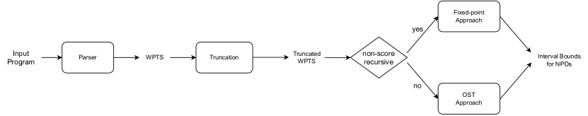
Figure 4. An overview of our method

Before we go into the details of the examples, we first present the workflow of our approaches. Given a probabilistic program $P$ and a measurable set $\mathcal{U}\in\Sigma_{\mathbb{R}^{|V_{\mathrm{p}}|}}$, the workflow of our approaches is shown in Fig. 4: First, our parser transforms the input program $P$ into its WPTS $\Pi$ in the form of († ‣ 2.2); Second, our approaches perform a truncation operation (to be introduced in Section 4.3) that restricts the WPTS $\Pi$ into the bounded range of program values so that whenever the program runs out of the range, our approaches directly have upper and lower bounds to over- and under-approximate the behaviour of the program outside the bounded range, the purpose of which is that a bounded range allows our approach to derive tight bounds via templates; Third, the truncated WPTS is further handled by our fixed-point or OST approach, depending on whether or not $\Pi$ is score-recursive, to generate polynomial bounds for expected weights at the termination of the program; Fourth, the interval bounds for the NPD $\mathsf{posterior}_{\Pi}(\mathcal{U})$ are calculated by the interval-bound analysis for expected weights. An illustration of our workflow is given in Fig. 4.

3.1. Pedestrian Random Walk

Consider the pedestrian random walk example  (Mak et al., 2021) in Fig. 3. In this example, a pedestrian is lost on the way home, and she only knows that she is away from her house at most $3$ km. Thus, she starts to repeatedly walk a uniformly random distance of at most $1$ km in either direction of the road, until reaching her house. Upon she arrives, an odometer tells that she has walked $1.1$ km totally. However, this odometer was once broken and the measured distance is normally distributed around the true distance with a standard deviation of $0.1$ km. The question of this example is: what is the posterior distribution of the starting point? This example is modeled as a non-parametric probabilistic program whose number of loop iterations is unbounded. In the program, the variable $start$ represents the starting point, $pos$ records the current position of the pedestrian, $step$ records the distance she walks in the next step, and $dis$ records the total distance the pedestrian travelled so far. The probabilistic branch in the loop body specifies that the pedestrian walks either forward or backward, both with probability $0.5$.

This program is non-score-recursive and was previously handled in (Beutner et al., 2022) by exhaustive recursion unrolling that has the path-explosion problem. To circumvent the path-explosion problem, in this work we propose a fixed-point theorem to establish constraints for this example, and solve the constraints by polynomial templates. To utilize the fact that polynomial approximation is usually accurate over a bounded range, during the solving of the polynomial templates, we restrict the behaviour of the program within a bounded range (e.g., $\{(pos,dis)\mid pos,dis\in[0,5]\}$) and over-approximate the expected weights outside the bounded range by an interval (e.g. $[0,2.1\times 10^{-330}]$). Note that here we omit the program variable $start$ as its value is determined once and has nothing to do with loop iterations. The solving of the polynomial template follows the previous approaches (Chakarov and Sankaranarayanan, 2013b; Chatterjee et al., 2018, 2016a) that consider linear/semidefinite programming. Our approach derives comparable bounds to the approach in Beutner et al. (2022) while our runtime is two-thirds of that of Beutner et al. (2022).

3.2. Phylogenetic Birth Model

Consider a simplified version of the phylogenetic birth model (Ronquist et al., 2021) in Fig. 6, where a species arises with a birth-rate $lambda$, and it propagates with a constant likelihood of $1.1$ at some time interval. This example is modelled as a probabilistic loop, where the variables $lambda,time,amount,wait$ stand for the birth rate of the species, the remaining propagation time, the current amount of the species and the propagation time to be spent, respectively. The variable $lambda$ is associated with a prior distribution, and the NPD problem is to infer its posterior distribution given the species evolution described by the loop. The WPTS of the program is given in Fig. 6.

This program cannot be handled by previous approaches (such as (Beutner et al., 2022; Gehr et al., 2020)) since it is a score-recursive program with an unbounded while loop and its score weight is greater than $1$. To see why such a score-recursive program is nontrivial to tackle, consider a simple loop where in each loop iteration, the loop terminates directly with probability $\frac{1}{2}$, and continues to the next loop iteration with the same probability. At the end of each loop iteration, a score command “score$(3)$” is executed. It follows that the normalising constant in NPD is equal to $\sum_{n=1}^{\infty}\mathbb{P}(T=n)\cdot 3^{n}=\sum_{n=1}^{\infty}(\frac{3}{2})^{n}=\infty$, so that the infinity makes the posterior distribution invalid. One can observe that in this example the main problem lies at the fact that the scaling speed of the likelihood weight (i.e., $3$) is higher than that for program termination (i.e., $\frac{1}{2}$).

To tackle the difficulty of having scores greater than $1$ in a loop iteration, we propose a novel multiplicative variant of Optional Stopping Theorem (OST) that addresses score statements. Based on our OST variant, we apply truncation and polynomial template solving as in the non-score-recursive case. For example, we can restrict the behaviour of the program within a bounded range such as $\{(lambda,time)\mid lambda\in[0,3]$ and $time\in[0,10]\}$, and over-approximate the expected weights outside the bounded range by an interval bound of polynomial functions derived from the same OST variant and polynomial-template method but without truncation. For the same reason as in Section 3.1, here we can safely omit the program variable $amount$. Our experimental result on this example shows that the derived bounds match the simulation result with $10^{6}$ samples.

⬇

$\mbox{\sl lambda}:=$ sample uniform$(0,2)$;

$\mbox{\sl time}:=10$; $\mbox{\sl amount}:=0$;

$\ell_{\mathrm{init}}:$ while $\mbox{\sl time}\geq 0$ do

$\mbox{\sl wait}:=$ sample uniform$(0,0.5)$;

$\mbox{\sl time}:=\mbox{\sl time}-\mbox{\sl wait}$;

if prob($0.5\cdot\mbox{\sl lambda}$) then

$\mbox{\sl birth}:=$ sample uniform($0,0.01$);

$\mbox{\sl amount}:=\mbox{\sl amount}+\mbox{\sl birth}$;

score($1.1$)

fi;

od;

return lambda

$\ell_{\mathrm{out}}:$

Figure 5. A Phylogenetic Birth Model

Figure 6. The WPTS of Phylogenetic Model

4. Theoretical Approaches

In this section, we present our theoretical approaches for interval-bound analysis of expected weights in the form $\llbracket\Pi\rrbracket_{\mathbf{v}}(\mathbb{R}^{|V_{\mathrm{p}}|})$, namely the fixed-point approach, the OST approach. To obtain tight results, we also introduce the truncation operation.

4.1. The Fixed-Point Approach

We review some basic concepts of lattice theory. Given a partial order $\sqsubseteq$ on a set $K$ and a subset $K^{\prime}\subseteq K,$ an upper bound of $K^{\prime}$ is an element $u\in K$ that is no smaller than every element of $K^{\prime}$, i.e., $\forall k^{\prime}\in K^{\prime}.~{}k^{\prime}\sqsubseteq u.$ Similarly, a lower bound for $K^{\prime}$ is an element $l$ that is no greater than every element of $K^{\prime},$ i.e. $\forall k^{\prime}\in K^{\prime}.~{}l\sqsubseteq k^{\prime}.$ The supremum of $K^{\prime},$ denoted by $\bigsqcup K^{\prime}$, is an element $u^{*}\in K$ such that $u^{*}$ is an upper-bound of $K^{\prime}$ and for every upper bound $u$ of $K^{\prime},$ we have $u^{*}\sqsubseteq u.$ Similarly, the infimum $\bigsqcap K^{\prime}$ is a lower bound $l^{*}$ of $K^{\prime}$ such that for every lower-bound $l$ of $K^{\prime},$ we have $l\sqsubseteq l^{*}.$ We define $\bot\!:=\!\bigsqcap K$ and $\top\!:=\!\bigsqcup K.$ In general, suprema and infima may not exist.

A partially-ordered set $(K,\sqsubseteq)$ is called a complete lattice if every subset $K^{\prime}\subseteq K$ has a supremum and an infimum. Given a partial order $(K,\sqsubseteq)$, a function $f:K\to K$ is called monotone if for every $k_{1}\sqsubseteq k_{2}$ in $K$, we have $f(k_{1})\sqsubseteq f(k_{2}).$

Given a complete lattice $(K,\sqsubseteq),$ a function $f:K\to K$ is called continuous if for every increasing chain $k_{0}\sqsubseteq k_{1}\sqsubseteq\ldots$ in $K,$ we have $f(\bigsqcup\{k_{n}\}_{n=0}^{\infty})=\bigsqcup\{f(k_{n})\}_{n=0}^{\infty},$ and cocontinuous if for every decreasing chain $k_{0}\sqsupseteq k_{1}\sqsupseteq\ldots$ of elements of $K,$ we have $f(\bigsqcap\{k_{n}\}_{n=0}^{\infty})=\bigsqcap\{f(k_{n})\}_{n=0}^{\infty}.$ An element $k\in K$ is called a fixed-point if $f(k)=k.$ Moreover, $k$ is a pre fixed-point if $f(k)\sqsubseteq k$ and a post fixed-point if $k\sqsubseteq f(k)$. The least fixed-point of $f$, denoted by $\mathrm{lfp}f,$ is the fixed-point that is no greater than every fixed-point under $\sqsubseteq.$ Analogously, the greatest fixed-point of $f$, denoted by $\mathrm{gfp}f$, is the fixed-point that is no smaller than all fixed-points.

Theorem 4.1 (Kleene (Sangiorgi, 2011)).

Let $(K,\sqsubseteq)$ be a complete lattice and $f:K\to K$ be an continuous function. Then, we have

$$\textstyle\mathrm{lfp}\ f={\textstyle\mathop{\bigsqcup}_{i\geq 0}}\left\{f^{(i)}(\bot)\right\}.$$

Analogously, if $f$ is cocontinuous, then we have

$$\textstyle\mathrm{gfp}\ f={\textstyle\mathop{\bigsqcap}_{i\geq 0}}\left\{f^{(i)}(\top)\right\}.$$

In this work, we apply the well-known Tarski’s fixed-point theorem.

Theorem 4.2 (Tarski (Tarski, 1955)).

Let $(K,\sqsubseteq)$ be a complete lattice and $f:K\to K$ a monotone function. Then, both $\mathrm{lfp}\ f$ and $\mathrm{gfp}\ f$ exist. Moreover, we have

$$\textstyle\mathrm{lfp}\ f=\mathop{\bigsqcap}\left\{x\ |\ f(x)\sqsubseteq x\right\}\mbox{ and }\mathrm{gfp}\ f=\mathop{\bigsqcup}\left\{x\ |\ x\sqsubseteq f(x)\right\}.$$

Based on Theorem 4.2, we present our fixed-point approach for non-score-recursive WPTS’s. Below we fix a non-score-recursive WPTS $\Pi$ in the form of († ‣ 2.2). Given a maximum finite value $M\in[0,\infty)$, we define a state function as a function $h:\Lambda\to[-M,M]$ such that for all $\mathbf{v}\in\mathbb{R}^{|V_{\mathrm{p}}|}$, we have that $h(\ell_{\mathrm{out}},\mathbf{v})\in[0,M]$. We denote the set of all state functions with maximum value $M$ by $\mathcal{K}_{M}$. We also use the usual partial order $\leq$ on $\mathcal{K}_{M}$ that is defined in the pointwise fashion, i.e., for any $h_{1},h_{2}\in\mathcal{K}_{M}$, $h_{1}\leq h_{2}$ iff $h_{1}(\Xi)\leq h_{2}(\Xi)$ for all $\Xi\in\Lambda$. It is straightforward to verify that $(\mathcal{K}_{M},\leq)$ is a complete lattice. For example, the top element $\top$ (resp. the bottom element $\bot$) in the set $\mathcal{K}_{M}$ is the constant function that maps every state $\Xi$ to $M$ (resp. $-M$), and the least upper bounds (resp. greatest lower bound) can be given via the pointwise infimum (resp. supremum), respectively.

To connect the complete lattice $(\mathcal{K}_{M},\leq)$ of state functions with expected weights (Definition 2.6), we define a special state function, called expected-weight function $\mbox{\sl ew}_{\Pi}$, by $\mbox{\sl ew}_{\Pi}(\ell_{\mathrm{init}},\mathbf{v}):=\llbracket\Pi\rrbracket_{\mathbf{v}}(\mathbb{R}^{|V_{\mathrm{p}}|})$, and omit the subscript $\Pi$ if it is clear from the context. Informally, $\mbox{\sl ew}_{\Pi}(\ell_{\mathrm{init}},\mathbf{v})$ is the expected weight of all program runs that start from $\mathbf{v}$ without the restriction of the subset $\mathcal{U}$. In this work, we consider the following monotone function over the complete lattice $(\mathcal{K}_{M},\leq)$.

Definition 4.3 (Expected-Weight Transformer).

Given a finite maximum value $M\in[1,\infty)$, the expected-weight transformer $\mbox{\sl ewt}_{\Pi}:\mathcal{K}_{M}\to\mathcal{K}_{M}$ is the higher-order function such that for each state function $h\in\mathcal{K}_{M}$ and state $(\ell,\mathbf{v})$, if $\tau=\langle\ell,\phi,F_{1},\dots,F_{k}\rangle$ is the unique transition that satisfies $\mathbf{v}\models\phi$ and $F_{j}=\langle\ell^{\prime}_{j},p_{j},\mbox{\sl upd}_{j},\mbox{\sl wt}_{j}\rangle$ for each $1\leq j\leq k$, then we have that

(1) $$\mbox{\sl ewt}_{\Pi}(h)(\ell,\mathbf{v})\,:=\,\begin{cases}\sum_{j=1}^{k}p_{j}\cdot\mathbb{E}_{\mathbf{r}}\left[{\mbox{\sl wt}_{j}(\mathbf{v},\mathbf{r})\cdot h(\ell^{\prime}_{j},\mbox{\sl upd}_{j}(\mathbf{v},\mathbf{r}))}\right]&\mbox{if }\ell\neq\ell_{\mathrm{out}}\\ 1&\mbox{otherwise}\end{cases}\enskip.$$

Here the expectation $\mathbb{E}_{\mathbf{r}}\left[{-}\right]$ is taken over a sampling valuation $\mathbf{r}$ that observes the independent joint probability distributions of all the sampling variables $r\in V_{\mathrm{r}}$.

Informally, given a state function $h$, the expected-weight transformer $\mbox{\sl ewt}_{\Pi}$ computes the expected weight $\mbox{\sl ewt}_{\Pi}(h)$ after one step of the WPTS execution. From the monotonicity of the Lebesgue integral (from the definition of expectation), we have that $\mbox{\sl ewt}_{\Pi}$ is monotone. Note that although the Lebesgue integral of a function $f$ usually requires measurability of the function, its preliminary definition is given via a supremum over simple functions not exceeding the function, and hence can be applied to all functions (including non-measurable functions) for which the monotonicity remains to be true. Therefore, we do not need to impose measurability here. In the following, we will omit the subscript $\Pi$ in $\mbox{\sl ewt}_{\Pi}$ if it is clear from the context.

Definition 4.4 (Potential Weight Functions).

A potential upper weight function (PUWF) is a function $h:\mathit{L}{}\times\mbox{\sl Val}_{V_{p}}\rightarrow\mathbb{R}$ that has the properties below:

• for all reachable states $(\ell,\mathbf{v})$ with $\ell\neq\ell_{\mathrm{out}}$, we have $\mbox{\sl ewt}({h})(\ell,\mathbf{v})\leq h(\ell,\mathbf{v})$;

• for all reachable states $(\ell,\mathbf{v})$ such that $\ell=\ell_{\mathrm{out}}$, we have $h(\ell,\mathbf{v})=1$.

Analogously, a potential lower weight function (PLWF) is a function $h:\mathit{L}{}\times\mbox{\sl Val}_{V_{p}}\rightarrow\mathbb{R}$ that satisfies the conditions (C1’) and (C2), for which the condition (C1’) is almost the same as (C1) except for that “$\mbox{\sl ewt}({h})(\ell,\mathbf{v})\leq h(\ell,\mathbf{v})$” is replaced with “$\mbox{\sl ewt}({h})(\ell,\mathbf{v})\geq h(\ell,\mathbf{v})$”.

Informally, a PUWF is a state function that satisfies the pre fixed-point condition of ewt at non-terminating locations, and equals one at the termination location. A PLWF is defined similarly, with the difference that we use the post fixed-point condition instead.

The following result lays the backbone of our fixed-point approach.

Theorem 4.5.

Let $\Pi$ be a non-score-recursive WPTS that is score-bounded by a positive real $M>0$. If the WPTS $\Pi$ has the AST property, then the expected-weight function ew is the unique fixed-point of the higher-order function ewt on the complete lattice $(\mathcal{K}_{\max\{M,1\}},\leq)$.

Proof sketch..

Let $M^{\prime}:=\max\{M,1\}$. We first prove that the expected-weight function ew is the least fixed-point of the higher-order function ewt. Then we prove that the expected-weight transformer $\mbox{\sl ewt}:\mathcal{K}_{M^{\prime}}\to\mathcal{K}_{M^{\prime}}$ is both continuous and cocontinuous. Finally, according to Theorem B.1, we prove the uniqueness that $\mathrm{lfp}\ \mbox{\sl ewt}(\ell,\mathbf{v})=\mathrm{gfp}\ \mbox{\sl ewt}(\ell,\mathbf{v})$, i.e., the fixed-point ew is unique. For the space limitation, we relegate the detailed proof for Theorem 4.5 to Appendix B.2. ∎

By a combination of Theorem 4.5 and Theorem 4.2, one has that it suffices to derive a pre fixed-point of ewt to obtain an upper bound for ew, and a post fixed-point to obtain a lower bound in the case of almost-sure termination of the program .

Theorem 4.6 (Fixed-Point Approach).

Let $\Pi$ be a non-score-recursive WPTS that is score-bounded by a finite value $M>0$. If the WPTS $\Pi$ has the AST property, then $\llbracket\Pi\rrbracket_{\mathbf{v}_{\mathrm{init}}}(\mathbb{R}^{|V_{\mathrm{p}}|})\leq h(\ell_{\mathrm{init}},\mathbf{v}_{\mathrm{init}})$ (resp. $\llbracket\Pi\rrbracket_{\mathbf{v}_{\mathrm{init}}}(\mathbb{R}^{|V_{\mathrm{p}}|})\geq h(\ell_{\mathrm{init}},\mathbf{v}_{\mathrm{init}})$) for any PUWF (resp. PLWF) $h$ over $\Pi$ and initial state $(\ell_{\mathrm{init}},\mathbf{v}_{\mathrm{init}})$, respectively.

Remark 1.

Notice that we always require a finite maximal value $M$ in our fixed-point approach. In general, our fixed-point approach cannot be applied to score-recursive Bayesian probabilistic programs, as in such a program a finite maximum weight $M$ may not exist.

4.2. The OST Approach

As stated in Remark 1, our fixed-point approach cannot handle score-recursive Bayesian probabilistic programs. To tackle score-recursive programs, we consider the adaption of Optional Stopping Theorem (OST) to our case. OST is a classical theorem in martingale theory that characterizes the relationship between the expected values initially and at a stopping time in a supermartingale. Below we first present the classical form of OST.

Theorem 4.7 (Optional Stopping Theorem (OST) (Williams, 1991)).

Let $\{X_{n}\}_{n=0}^{\infty}$ be a supermartingale adapted to a filtration $\mathcal{F}=\{\mathcal{F}_{n}\}_{n=0}^{\infty}$, and $\kappa$ be a stopping time w.r.t. the filtration $\mathcal{F}$. Then the following condition is sufficient to ensure that $\mathbb{E}\left(|X_{\kappa}|\right)<\infty$ and $\mathbb{E}\left(X_{\kappa}\right)\leq\mathbb{E}(X_{0})$:

• $\mathbb{E}(\kappa)<\infty$, and

• (bounded difference) there exists a constant $C>0$ such that for all $n\geq 0$, $|X_{n+1}-X_{n}|\leq C$ holds almost surely.

In our NPD problem, as the score statements accumulate weights in a multiplicative fashion, the classical OST cannot be applied since the bounded difference condition may be violated. To address this difficulty, we propose a novel variant of OST that tackles the multiplicative feature from score statements.

Theorem 4.8 (OST Variant).

Let $\{X_{n}\}_{n=0}^{\infty}$ be a supermartingale adapted to a filtration $\mathcal{F}=\{\mathcal{F}_{n}\}_{n=0}^{\infty}$, and $\kappa$ be a stopping time w.r.t. the filtration $\mathcal{F}$. Then the following condition $(\mho)$ is sufficient to ensure that $\mathbb{E}\left(|X_{\kappa}|\right)<\infty$ and $\mathbb{E}\left(X_{\kappa}\right)\leq\mathbb{E}(X_{0})$:

• There exist integers $b_{1},b_{2}>0$ and real numbers $c_{1}>0,c_{2}>c_{3}>0$ such that (i) $\mathbb{P}(\kappa>n)\leq c_{1}\cdot e^{-c_{2}\cdot n}$ for sufficiently large $n\in\mathbb{N}$, and (ii) for all $n\in\mathbb{N}$, $\left|X_{n+1}-X_{n}\right|\leq b_{1}\cdot n^{b_{2}}\cdot e^{c_{3}\cdot n}$ holds almost surely.

Our OST variant extends the classical OST with the relaxation that we allow the magnitude of the next random variable $X_{n+1}$ to be bounded by that of $X_{n}$ with a multiplicative factor $e^{c_{3}}$, which corresponds to the multiplicative feature from score statements. The intuition of the theorem is that to cancel the effect of the multiplicative factor, we require in extra the exponential decrease in $\mathbb{P}(\kappa>n)\leq c_{1}\cdot e^{-c_{2}\cdot n}$. The proof resembles (Wang et al., 2019, Theorem 5.2) and is relegated to Section B.3.

Below we show how our OST variant can be applied to handle score-recursive WPTS’s. Fix a WPTS $\Pi$ in the form of († ‣ 2.2). In the rest of this subsection, we reuse the expected-weight transformer ewt defined in Definition 4.3 and potential weight functions given in Definition 4.4. The slight difference is that for the expected-weight transformer in the context of a score-recursive WPTS, we consider that the weight function $\mbox{\sl wt}_{j}$ before termination may not be constantly $1$.

To apply our multiplicative OST variant, we impose a bounded update requirement as in (Wang et al., 2019). A WPTS $\Pi$ has the bounded update property if there exists a constant $\varkappa>0$ such that for every reachable state $(\ell,\mathbf{v})$, if $\tau=\langle\ell,\phi,F_{1},\dots,F_{k}\rangle$ is the unique transition with each fork $F_{j}=\langle\ell^{\prime}_{j},p_{j},\mbox{\sl upd}_{j},\mbox{\sl wt}_{j}\rangle$ such that $\mathbf{v}\models\phi$, then we have that $\forall\mathbf{r}\in\textsf{supp}\left({\mathcal{D}}\right)\,~{}\forall x\in V_{\mathrm{p}},~{}~{}|\mbox{\sl upd}_{j}(\mathbf{v},\mathbf{r})(x)-\mathbf{v}(x)|\leq\varkappa$.

We apply our OST variant (Theorem 4.8) in a way similar to (Wang et al., 2019, Theorem 6.10 and Theorem 6.12) to obtain the main theorem for our OST-based approach. To be more precise, we construct a stochastic process from a PUWF (or the negative of a PLWF) and show that the stochastic process is a supermartingale and the condition $(\mho)$ is fulfilled. The statement of the theorem is as follows.

Theorem 4.9 (OST Approach).

Let $\Pi$ be a score-recursive WPTS that has the bounded update property. Suppose that there exist real numbers $c_{1}>0$ and $c_{2}>c_{3}>0$ such that

• $\mathbb{P}(T>n)\leq c_{1}\cdot e^{-c_{2}\cdot n}$ for sufficiently large $n\in\mathbb{N}$, and

• for each score function wt in $\Pi$ we have $|\mbox{\sl wt}|\leq e^{c_{3}}$.

Then for any PUWF (resp. PLWF) $h$ over $\Pi$, we have that $\llbracket\Pi\rrbracket_{\mathbf{v}_{\mathrm{init}}}(\mathbb{R}^{|V_{\mathrm{p}}|})\leq h(\ell_{\mathrm{init}},\mathbf{v}_{\mathrm{init}})$ (resp. $\llbracket\Pi\rrbracket_{\mathbf{v}_{\mathrm{init}}}(\mathbb{R}^{|V_{\mathrm{p}}|})\geq h(\ell_{\mathrm{init}},\mathbf{v}_{\mathrm{init}})$) for any initial state $(\ell_{\mathrm{init}},\mathbf{v}_{\mathrm{init}})$, respectively.

Proof Sketch..

For the upper bounds, we define the stochastic process $\{X_{n}\}_{n=0}^{\infty}$ as $X_{n}:=h(\ell_{n},\mathbf{v}_{n})$ where $(\ell_{n},\mathbf{v}_{n})$ is the program state at the $n$th step of a program run. Then we construct a stochastic process $\{Y_{n}\}_{n=0}^{\infty}$ such that $Y_{n}:=X_{n}\cdot\prod_{i=0}^{n-1}W_{i}$ where $W_{i}$ is the weight at the $i$th step of the program run. We consider the termination time $T$ of $\Pi$ and prove that $\{Y_{n}\}_{n=0}^{\infty}$ satisfies the prerequisites of our OST variant (Theorem 4.8). This proof depends on the assumption that $\Pi$ has concentration and bounded update properties, and the score functions in $\Pi$ are also bounded (Item 2, Theorem 4.9)). Then by applying Theorem 4.8, we obtain that $\mathbb{E}\left[{Y_{T}}\right]\leq\mathbb{E}\left[{Y_{0}}\right]$. By (C2) in Definition 4.4, we have that $Y_{T}=h(\ell_{T},\mathbf{v}_{T})\cdot\prod_{i=0}^{T-1}W_{i}=\widehat{w}_{T}$. Thus, we have that $\llbracket\Pi\rrbracket_{\mathbf{v}_{\mathrm{init}}}(\mathbb{R}^{|V_{\mathrm{p}}|})=\mathbb{E}_{\mathbf{v}_{\mathrm{init}}}\left[{\widehat{w}_{T}}\right]=\mathbb{E}\left[{\prod_{i=0}^{T-1}W_{i}}\right]\leq\mathbb{E}\left[{Y_{0}}\right]=h(\ell_{\mathrm{init}},\mathbf{v}_{\mathrm{init}})$. For the lower bounds, the proof is similar. The more detailed proof is relegated to Section B.4. ∎

4.3. Truncation over WPTS’s

In the following, we propose a truncation operation for a WPTS that restricts the value of every program variable in the WPTS to a prescribed bounded range. We consider that a bounded range for a program variable could be either $[-R,R]$ ($R>0$), or $[0,R],[-R,0]$ if the value of the program variable is guaranteed to be non-negative or non-positive.

To present our truncation operation, we define the technical notions of truncation and approximation functions. A truncation function $\mathcal{B}$ is a function that maps every program variable $x\in V_{\mathrm{p}}$ to a bounded interval $\mathcal{B}(x)$ in $\mathbb{R}$ that specifies the bounded range of the variable $x$. We denote by $\Phi_{\mathcal{B}}$ the formula $\bigwedge_{x\in V_{\mathrm{p}}}x\in\mathcal{B}(x)$ for a truncation function $\mathcal{B}$. An approximation function is a function $\mathcal{M}:\mathbb{R}^{|V_{\mathrm{p}}|}\to[0,\infty)$ such that each $\mathcal{M}(\mathbf{v})$ ($\mathbf{v}\in\mathbb{R}^{|V_{\mathrm{p}}|}$) is intended to be an over- or under-approximation of the expected weight $\llbracket\Pi\rrbracket_{\mathbf{v}}(\mathbb{R}^{|V_{\mathrm{p}}|})$ outside the bounded range specified by $\Phi_{\mathcal{B}}$. The truncation operation is given by the following definition.

Definition 4.10 (Truncation Operation).

Let $\Pi$ be a WPTS in the form of († ‣ 2.2). Given a truncation function $\mathcal{B}$ and an approximation function $\mathcal{M}$, the truncated WPTS $\Pi_{\mathcal{B},\mathcal{M}}$ w.r.t. $\mathcal{B}$ and $\mathcal{M}$ is defined as $\Pi_{\mathcal{B},\mathcal{M}}:=(V_{\mathrm{p}},V_{\mathrm{r}},L\cup\{\#\},\ell_{\mathrm{init}},\ell_{\mathrm{out}},\mu_{\mathrm{init}},\mathcal{D},\mathfrak{T}_{\mathcal{B},\mathcal{M}})$ where $\#$ is a fresh deadlock location and the transition relation $\mathfrak{T}_{\mathcal{B},\mathcal{M}}$ is given by

$$\mathfrak{T}_{\mathcal{B},\mathcal{M}}:=\{\langle\ell,\phi\wedge\Phi_{\mathcal{B}},F_{1},\dots,F_{k}\rangle\mid\langle\ell,\phi,F_{1},\dots,F_{k}\rangle\in\mathfrak{T}\mbox{ and }\ell\neq\ell_{\mathrm{out}}\}$$

(‡) $$\quad\cup\{\langle\ell,\phi\wedge(\neg\Phi_{\mathcal{B}}),F^{\mathcal{M},\sharp}_{1},\dots,F^{\mathcal{M},\sharp}_{k}\rangle\mid\langle\ell,\phi,F_{1},\dots,F_{k}\rangle\in\mathfrak{T}\mbox{ and }\ell\neq\ell_{\mathrm{out}}\}$$

$$\quad\cup\{\langle\ell_{\mathrm{out}},\mathbf{true},F_{\ell_{\mathrm{out}}}\rangle,\langle\sharp,\mathbf{true},F_{\sharp}\rangle\}$$

for which (a) we have $F_{\ell}:=\langle\ell,1,\mbox{\sl id},\overline{1}\rangle$ ($\ell\in\{\ell_{\mathrm{out}},\sharp\}$) where id is the identity function and $\overline{1}$ is the constant function that always takes the value $1$, and (b) for a fork $F=\langle\ell^{\prime},p,\mbox{\sl upd},\mbox{\sl wt}\rangle$ in the original WPTS $\Pi$ we have $F^{\mathcal{M},\sharp}:=F$ if $\ell^{\prime}=\ell_{\mathrm{out}}$ and $F^{\mathcal{M},\sharp}:=\langle\sharp,p,\mbox{\sl upd},\mathcal{M}\rangle$ otherwise.

Thus, the truncated WPTS is obtained from the original one by first restraining each transition to the bounded range $\Phi_{\mathcal{B}}$ and then redirecting to the fresh deadlock location $\sharp$ all the situations jumping out of the bounded range and not going to the termination location. To make the truncated WPTS deterministic and total, we add the self-loop $\langle\sharp,\mathbf{true},F_{\sharp}\rangle$. Our main theorem shows that by choosing an appropriate approximation function $\mathcal{M}$ in the truncation, one can obtain upper/lower approximation of the original WPTS.

Theorem 4.11.

Let $\Pi$ be a WPTS in the form of († ‣ 2.2), $\mathcal{B}$ a truncation function and $\mathcal{M}$ an approximation function. Suppose that the following condition ($\ast$) holds:

• for each fork $F^{M,\sharp}=\langle\sharp,p,\mbox{\sl upd},\mathcal{M}\rangle$ in the truncated WPTS $\Pi_{\mathcal{B},\mathcal{M}}$ that is derived from some fork $F=\langle\ell^{\prime},p,\mbox{\sl upd},\mbox{\sl wt}\rangle$ with the source location $\ell$ in the original WPTS (see sentence (b) in Definition 4.10), we have that $\llbracket\Pi\rrbracket_{\mathbf{v}}(\mathbb{R}^{|V_{\mathrm{p}}|})\leq\mathcal{M}(\mathbf{v})$ for all $\mathbf{v}$ such that the state $(\ell,\mathbf{v})$ is reachable and $\mathbf{v}\not\models\Phi_{\mathcal{B}}$.

Then $\llbracket\Pi\rrbracket_{\mathbf{v}_{\mathrm{init}}}(\mathbb{R}^{|V_{\mathrm{p}}|})\leq\llbracket\Pi_{\mathcal{B},\mathcal{M}}\rrbracket_{\mathbf{v}_{\mathrm{init}}}(\mathbb{R}^{|V_{\mathrm{p}}|})$ for all initial program valuations $\mathbf{v}_{\mathrm{init}}$. Analogously, if it holds the condition ($\star$) which is almost the same as ($\ast$) except for that “$\llbracket\Pi\rrbracket_{\mathbf{v}}(\mathbb{R}^{|V_{\mathrm{p}}|})\leq\mathcal{M}(\mathbf{v})$” is replaced with “$\llbracket\Pi\rrbracket_{\mathbf{v}}(\mathbb{R}^{|V_{\mathrm{p}}|})\geq\mathcal{M}(\mathbf{v})$”, then we have $\llbracket\Pi\rrbracket_{\mathbf{v}_{\mathrm{init}}}(\mathbb{R}^{|V_{\mathrm{p}}|})\geq\llbracket\Pi_{\mathcal{B},\mathcal{M}}\rrbracket_{\mathbf{v}_{\mathrm{init}}}(\mathbb{R}^{|V_{\mathrm{p}}|})$ for all initial program valuations $\mathbf{v}_{\mathrm{init}}$.

The theorem above states that if the approximation function gives correct bounds for the expected weights of the original WPTS outside the bounded range, then the bounds for the expected weights of the truncated WPTS are also correct bounds for the expected weights of the original WPTS. The detailed proof is relegated to Appendix C.

Example 4.12.

Recall the Pedestrian example in Fig. 3, here we make truncation to this example and generate its truncated WPTS. The truncation function $\mathcal{B}$ is defined such that $\mathcal{B}(pos)=[0,5]$, $\mathcal{B}(dis)=[0,5]$, so $\Phi_{\mathcal{B}}=0\leq pos\leq 5\wedge 0\leq dis\leq 5$. Following the truncation operation in (${\ddagger}$) from Definition 4.10, we can obtain $\Pi_{\mathcal{B},\mathcal{M}}$ as shown in Fig. 7.∎

Figure 7. The Truncated WPTS of Pedestrian

5. Algorithmic Approaches

In this section, we present algorithmic implementation of our theoretical approaches in Section 4. We first have some assumptions on the input probabilistic program:

• To enable the exact calculation of the integrals over the probability density functions in a Bayesian probabilistic program possible, we assume that every probability density function in a sampling statement is a polynomial. Likewise, in score-recursive programs, we require that the probability density function in any score statement is polynomial. Our approach can handle non-polynomial density functions in sampling and score statements by having their polynomial approximations, for which we leave as a future work.

• To capture all possible program executions, we assume that the input probabilistic program is accompanied with invariants (see e.g. (Chakarov and Sankaranarayanan, 2013a; Sankaranarayanan et al., 2004)) to over-approximate reachable states. We follow  (Colón et al., 2003; Sankaranarayanan et al., 2004) to consider affine invariants. An affine invariant for a WPTS is a map $I$ that assigns to each location $\ell$ a (conjunctive) system $I(\ell)$ of affine inequalities such that for all reachable states $(\ell,\mathbf{v})$, every affine inequality in $I(\ell)$ holds w.r.t the program values given in the program valuation $\mathbf{v}$.

We also present the high-level technical setting of our algorithms. Consider an input WPTS $\Pi$ in the form of († ‣ 2.2). Recall the normalising constant $Z_{\Pi}$ in Definition 2.7. To tighten the interval bounds for $Z_{\Pi}$, we split the set $\mathcal{V}:=\textsf{supp}\left({\mu_{\mathrm{init}}}\right)$ of initial program valuations into $m\geq 1$ disjoint partitions $\mathcal{V}_{1},\dots,\mathcal{V}_{m}$ such that $\mathcal{V}=\bigcup_{i=1}^{m}\mathcal{V}_{i}$ and $\mathcal{V}_{i}\cap\mathcal{V}_{j}=\emptyset$ for any $i\neq j\in[1,m]$. Our algorithms tackle each $\mathcal{V}_{i}$ ($1\leq i\leq m$) separately to obtain polynomial interval bounds $[l_{i},u_{i}]$ (where $l_{i},u_{i}$ are polynomials) such that $l_{i}(\mathbf{v})\leq\llbracket\Pi\rrbracket_{\mathbf{v}}(\mathbb{R}^{|V_{\mathrm{p}}|})\leq u_{i}(\mathbf{v})$ for all $\mathbf{v}\in\mathcal{V}_{i}$. It follows that the interval bound $[l_{Z},u_{Z}]$ for $Z_{\Pi}$ can be derived by integrals of polynomial bounds over all $\mathcal{V}_{i}$’s, that is,

($$\clubsuit l_{Z}:=\sum_{i=1}^{m}\int_{\mathcal{V}_{i}}l_{i}(\mathbf{v})\mu_{\mathrm{init}}(\mathrm{d}\mathbf{v})\leq Z_{\Pi}=\sum_{i=1}^{m}\int_{\mathcal{V}_{i}}\llbracket\Pi\rrbracket_{\mathbf{v}}(\mathbb{R}^{|V_{\mathrm{p}}|})\cdot\mu_{\mathrm{init}}(\mathrm{d}\mathbf{v})\leq\sum_{i=1}^{m}\int_{\mathcal{V}_{i}}u_{i}(\mathbf{v})\mu_{\mathrm{init}}(\mathrm{d}\mathbf{v})=:u_{Z}.$$)

Given a measurable set $\mathcal{U}\in\Sigma_{\mathbb{R}^{|V_{\mathrm{p}}|}}$, the interval bounds $[l_{\mathcal{U}},u_{\mathcal{U}}]$ for the unnormalised posterior distribution $\llbracket\Pi\rrbracket(\mathcal{U})$ (in Definition 2.7) can be obtained analogously by deriving polynomial bounds for $\llbracket\Pi_{\mathcal{U}}\rrbracket_{\mathbf{v}}(\mathbb{R}^{|V_{\mathrm{p}}|})$ (see Proposition 2.8).

Below we present our algorithmic methods to deriving interval bounds for the normalising constant. The unnormalised posterior distribution can be derived in the same manner. Our algorithms are template-based and have the following stages:

Stage 1: Input. First, our algorithms receive a WPTS $\Pi$ parsed from a Bayesian probabilistic program $P$ written in our PPL and an affine invariant $I$ for the WPTS as the basic input. Besides, the algorithms receive as auxiliary inputs a truncation function $\mathcal{B}$ and two approximation functions $\mathcal{M}_{\mathrm{up}},\mathcal{M}_{\mathrm{low}}$ that respectively fulfill the conditions ($\ast$), ($\star$) in the statement of Theorem 4.11. The truncation function is represented by the bounded intervals for each program variable, and the approximation functions are derived either from the score function at the termination of a non-score-recursive program or by applying our OST variant directly to a score-recursive program (without truncation). We also have two parameters $d,m$, for which $d$ is the degree of our polynomial template and $m$ is the number of partitions for the set $\mathcal{V}$ of initial program valuations (refer to ($\clubsuit$ ‣ 5)).

Moreover, if the program $P$ is non-score-recursive and its score function $g$ at the termination is non-polynomial, our algorithms take as extra inputs a (piecewise) polynomial approximation $g^{\prime}$ of $g$ and an error bound $\epsilon>0$ such that $|g(\mathbf{v})-g^{\prime}(\mathbf{v})|\leq\epsilon$ for all $\mathbf{v}\in B^{\prime}$ ($B^{\prime}$ is the extended bounded range of program variables that derived from a one-step program run and the truncation function $\mathcal{B}$, which will be introduced in Step A1 below).

Stage 2: Partition and Truncation. Next, our algorithms fetch the set $\mathcal{V}=\textsf{supp}\left({\mu_{\mathrm{init}}}\right)$ from the WPTS $\Pi$, partition it into $m$ disjoint subsets $\mathcal{V}_{1},\dots,\mathcal{V}_{m}$ and construct a set $\mathcal{W}=\{\mathbf{v}_{1},\dots,\mathbf{v}_{m}\}$ such that each $\mathbf{v}_{i}\in\mathcal{V}_{i}$. Our algorithms then perform the truncation operation to $\Pi$ w.r.t the input truncation function $\mathcal{B}$ and approximation functions $\mathcal{M}_{\mathrm{up}},\mathcal{M}_{\mathrm{low}}$. To synthesize upper bounds for expected weights, we take the truncation w.r.t $\mathcal{B}$ and $\mathcal{M}_{\mathrm{up}}$ to generate a truncated WPTS $\Pi_{\mathcal{B},\mathcal{M}_{\mathrm{up}}}$. For lower bounds, we generate the truncated WPTS $\Pi_{\mathcal{B},\mathcal{M}_{\mathrm{low}}}$.

Example 5.1.

Recall the Pedestrian example in Section 3.1 and its WPTS $\Pi$ in Fig. 3. We derive an invariant $I$ simply from the loop guard so that $I(\ell_{\mathrm{init}})=pos\geq 0$ and $I(\ell_{\mathrm{out}})=pos<0$. The truncation function $\mathcal{B}$ is defined such that $\mathcal{B}(pos)=[0,5]$ and $\mathcal{B}(dis)=[0,5]$. We pick the constant approximation functions $\mathcal{M}_{\mathrm{up}}=2.1\times 10^{-330}$ and $\mathcal{M}_{\mathrm{low}}=0$ to bound the expected weights beyond the truncated range, so that we obtain two truncated WPTSs $\Pi_{\mathcal{B},\mathcal{M}_{\mathrm{up}}}$ and $\Pi_{\mathcal{B},\mathcal{M}_{\mathrm{low}}}$ which are similar to that in Fig. 7. We also choose the algorithm parameters as $d=1$ and $m=30$. Since the program is non-score-recursive and its score function $g$ at the termination is non-polynomial (i.e., $g(dis)=pdf(normal(1.1,0.1),dis)$), we choose a polynomial approximation $g^{\prime}$ of $g$ with the error bound $\epsilon=10^{-5}$. We obtain the set $\mathcal{V}=\{(pos,dis)\mid pos\in[0,3],dis=0\}$. Since the value of $dis$ in $\mathcal{V}$ is fixed, we partition $\mathcal{V}$ uniformly into $m=30$ disjount subsets on the dimension $pos$, i.e., $\mathcal{V}_{1}=\{(pos,dis)\mid pos\in[0,0.1],dis=0\},\dots,\mathcal{V}_{30}=\{(pos,dis)\mid pos\in[2.9,3],dis=0\}$. We calculate the midpoints of the dimension $pos$ for all $\mathcal{V}_{i}$’s, and construct the set $\mathcal{W}=\{(0.05,0),(0.15,0),\dots,(2.95,0)\}$.∎

Stage 3: Template Solving. Then our algorithms establish $d$-degree polynomial templates for $\Pi_{\mathcal{B},\mathcal{M}_{\mathrm{up}}}$ and $\Pi_{\mathcal{B},\mathcal{M}_{\mathrm{low}}}$, and synthesize polynomial upper and lower bounds for the expected weights $\llbracket\Pi_{\mathcal{B},\mathcal{M}_{\mathrm{up}}}\rrbracket_{\mathbf{v}_{i}}(\mathbb{R}^{|V_{\mathrm{p}}|})$ and $\llbracket\Pi_{\mathcal{B},\mathcal{M}_{\mathrm{low}}}\rrbracket_{\mathbf{v}_{i}}(\mathbb{R}^{|V_{\mathrm{p}}|})$ for each initial program valuation $\mathbf{v}_{i}\in\mathcal{V}_{i}$ in $\mathcal{W}$ by solving the templates w.r.t the PUWF and PLWF constraints (i.e., (C1), (C2), (C1’) from Definition 4.4), respectively. The correctness of this stage follows from Theorem 4.6 and Theorem 4.9.

Note that Theorem 4.6 and Theorem 4.9 have prerequisites and we check these prerequisites in a succinct fashion as follows. For Theorem 4.6, we manually verify the AST property by the approaches of (Chakarov and Sankaranarayanan, 2013b; Chatterjee et al., 2016b), and check the score-bounded property by a direct manual inspection. For Theorem 4.9, we check the condition (E1) by approaches such as (Chatterjee et al., 2018; Wang et al., 2021b), the condition (E2) by a manual examination, and the bounded update property by simple check on whether the update value is bounded by a constant. The checking of the AST can be automated by template-based approaches (Chakarov and Sankaranarayanan, 2013b; Chatterjee et al., 2016b), and other simple prerequisites can be easily automated (via e.g. SMT solvers). We leave a fuller implementation that incorporate these features as a future work.

Below we present the detailed steps (Step A1 – A4) of our template solving.

Step A1. Consider the truncated WPTS $\Pi_{\mathcal{B},\mathcal{M}_{\mathrm{up}}}$ (to derive an upper bound) or $\Pi_{\mathcal{B},\mathcal{M}_{\mathrm{low}}}$ (to derive a lower bound). We denote the bounded range from the truncation function $\mathcal{B}$ by $B:=\{\mathbf{v}\mid\mathbf{v}(x)\in\mathcal{B}(x)\mbox{ for all }x\in V_{\mathrm{p}}\}$. In this step, both of our algorithms compute an extended bounded range $B^{\prime}$ such that any program valuation from a one-step execution of the WPTS under any current program valuation in $B$ falls in $B^{\prime}$. Formally, the extended bounded range $B^{\prime}$ satisfies that for every location $\ell$, program valuation $\mathbf{v}\in B$, transition $\tau=\langle\ell,\phi,F_{1},F_{2},\dots,F_{k}\rangle$, fork $F_{j}=\langle\ell^{\prime}_{j},p_{j},\mbox{\sl upd}_{j},\mbox{\sl wt}_{j}\rangle$ in $\tau$ and sampling valuation $\mathbf{r}\in\textsf{supp}\left({\mathcal{D}}\right)$, we have that $\mbox{\sl upd}_{j}(\mathbf{v},\mathbf{r})\in B^{\prime}$. Our algorithms determine the extended bounded range $B^{\prime}$ by examining the assignment statements in the truncated WPTS $\Pi_{\mathcal{B},\mathcal{M}_{\mathrm{up}}}$. The purpose to have a superset $B^{\prime}$ of the original bounded range $B$ is to reduce the runtime in the solving of the template, see Step A3 below.

Example 5.2.

Recall Example 5.1, the bounded range from the truncation function $\mathcal{B}$ is denoted by $B=\{(pos,dis)\mid pos\in[0,5],dis\in[0,5]\}$. For $\Pi_{\mathcal{B},\mathcal{M}_{\mathrm{up}}}$ or $\Pi_{\mathcal{B},\mathcal{M}_{\mathrm{low}}}$, the extended bounded range is given by $B^{\prime}=\{(pos,dis)\mid pos\in[-1,6],dis\in[0,6]\}$.∎

Step A2. In this step, at each location $\ell\not\in\{\ell_{\mathrm{out}},\sharp\}$, our algorithms set up a $d$-degree polynomial template $h_{\ell}$ over the program variables $V_{\mathrm{p}}$. Each template $h_{\ell}$ is a summation of all monomials of degree no more than $d$ and each monomial is multiplied with a fresh unknown coefficient as a parameter to be resolved. For $\ell\in\{\ell_{\mathrm{out}},\sharp\}$, our algorithms assume $h_{\ell}\equiv 1$.

Example 5.3.

Recall Example 5.1, the algorithm parameter $d=1$. For either $\Pi_{\mathcal{B},\mathcal{M}_{\mathrm{up}}}$ or $\Pi_{\mathcal{B},\mathcal{M}_{\mathrm{low}}}$, we construct a $1$-degree polynomial template at the location $\ell_{\mathrm{init}}$, i.e., $h_{\ell_{\mathrm{init}}}(pos,dis)=a_{1}\cdot pos+a_{2}\cdot dis+a_{3}$ where $a_{1},a_{2},a_{3}\in\mathbb{R}$ are unknown coefficients to be resolved, and let $h_{\ell_{\mathrm{out}}}=h_{\ell_{\sharp}}=1$.∎

Step A3. In this step, our algorithms establish constraints for the templates $h_{\ell}$’s from (C1), (C1’) in Definition 4.4 (as (C2) is satisfied by the construction of $h_{\ell}$ in the previous step). For upper bounds on expected weights, our algorithms have the following relaxed constraints of (C1) to synthesize a PUWF over $\Pi_{\mathcal{B},M_{up}}$:

• For every location $\ell\in\mathit{L}\setminus\{\ell_{\mathrm{out}},\sharp\}$ and program valuation $\mathbf{v}\in I(\ell)\cap B$, we have that $\mbox{\sl ewt}(h)(\ell,\mathbf{v})\leq h(\ell,\mathbf{v})$.

• For every location $\ell\in\mathit{L}\setminus\{\ell_{\mathrm{out}},\sharp\}$ and program valuation $\mathbf{v}\in I(\ell)\cap(B^{\prime}\setminus B)$, we have that $\mathcal{M}_{\mathrm{up}}(\mathbf{v})\leq h(\ell,\mathbf{v})$.

For lower bounds over $\Pi_{\mathcal{B},M_{low}}$, our algorithms have the relaxed PLWF constraints (D1’) and (D2’) which are obtained from (D1) and resp. (D2) by replacing “$\mbox{\sl ewt}(h)(\ell,\mathbf{v})\leq h(\ell,\mathbf{v})$” with “$\mbox{\sl ewt}(h)(\ell,\mathbf{v})\geq h(\ell,\mathbf{v})$” in (D1) and resp. “$\mathcal{M}_{\mathrm{up}}(\mathbf{v})\leq h(\ell,\mathbf{v})$” with “$\mathcal{M}_{\mathrm{low}}(\mathbf{v})\geq h(\ell,\mathbf{v})$” in (D2), respectively. We have that (D1) and (D2) together ensure (C1) since $\mathcal{M}_{\mathrm{up}}(\mathbf{v})\leq h(\ell,\mathbf{v})$ implies that $\mbox{\sl ewt}(h)(\ell,\mathbf{v})\leq h(\ell,\mathbf{v})$ for every location $\ell\in\mathit{L}\setminus\{\ell_{\mathrm{out}},\sharp\}$ and program valuation $\mathbf{v}\in I(\ell)\cap(B^{\prime}\setminus B)$. The same holds for (D1’) and (D2’).

Note that in (D1), the calculation of the value $\mbox{\sl ewt}(h)(\ell,\mathbf{v})$ has the piecewise nature that different sampling valuations $\mathbf{r}$ may cause the next program valuation to be within or outside the bounded range, and to satisfy or violate the guards of the transitions in the WPTS. In our algorithms, we have a fine-grained treatment for (D1) that enumerates all possible situations for a sampling valuation $\mathbf{r}$ that satisfy different guards of the WPTS in the calculation of $\mbox{\sl ewt}(h)(\ell,\mathbf{v})$, for which we use an SMT solver (e.g., Z3 (De Moura and Bjørner, 2008)) to compute the situations. As for (D2), we use (D2) to avoid handling the piecewise feature in the computation of $\mbox{\sl ewt}(h)(\ell,\mathbf{v})$ from within/outside the bounded range (i.e., the computation is a direct computation over a single-piece polynomial), so that the amount of computation of $\mbox{\sl ewt}(h)(\ell,\mathbf{v})$ is reduced by ignoring the piecewise feature. The use of (D2) to reduce the computation is the aim of introducing an extended bounded range in Step A1. The same also holds for (D1’) and (D2’).

If $\Pi$ is non-score-recursive and the score function $g$ at termination is non-polynomial, our algorithms replace $g$ in the expression $\mbox{\sl ewt}(h)(\ell,\mathbf{v})$ with its polynomial approximation $g^{\prime}$.

Example 5.4.

Recall Example 5.1–Example 5.3, the bounded range $\mathbb{D}_{1}=I(\ell_{\mathrm{init}})\cap B$ in (D1) is defined such that $pos\in[0,5]\wedge dis\in[0,5]$. Consider to derive upper bounds from $\Pi_{\mathcal{B},\mathcal{M}_{\mathrm{up}}}$. We make a fine-grained treatment for (D1) by splitting the range $\mathbb{D}_{1}$ and enumerating all possible situations for the sampling valuation $\textbf{sample uniform}(0,1)$ that the next program valuation satisfies or violates the loop guard “$pos\geq 0$”. In detail, $\mathbb{D}_{1}$ is split into $\mathbb{D}_{11}=\{(pos,dis)\mid pos\in[0,1),dis\in[0,5]\}$ and $\mathbb{D}_{12}=\{(pos,dis)\mid pos\in(1,5],dis\in[0,5]\}$, where $\mathbb{D}_{11}$ stands for the situation that with different sampling valuations the next program valuation may satisfy the loop guard (so that the next location is $\ell_{\mathrm{init}}$) or violate the loop guard (so that the next location is directed to $\ell_{\mathrm{out}}$), and $\mathbb{D}_{12}$ stands for the situation that the next program valuation will definitely satisfy the loop guard and the next location is $\ell_{\mathrm{init}}$. For the non-polynomial score function $g$ at the termination of the example, we replace it with a polynomial approximation $g^{\prime}$ under the error bound $10^{-5}$.

We first show the PUWF constraints for $\Pi_{\mathcal{B},\mathcal{M}_{\mathrm{up}}}$. Recall that the program has two probabilistic branches with probability $0.5$. When the current program valuation is in $\mathbb{D}_{11}$, we observe that

• if the loop takes the branch $pos:=pos+step$, then the next value of $pos$ remains to be non-negative and the loop continues, and

• if the loop takes the branch $pos:=pos-step$, then it is both possible that the next value of $pos$ satisfy or violate the loop guard, depending on the exact value of $step\in[0,1]$.

Then we have the constraint (D1.1) over $\mathbb{D}_{11}$ that has expectation over a piecewise function on $step$ derived from whether the loop terminates in the next iteration or not, as follows:

• $\forall pos,dis.$ $pos\in[0,1)\wedge dis\in[0,5]\Rightarrow$

  $$0.5\cdot\mathbb{E}_{step}\left[{[pos-step\geq 0]\cdot h_{\ell_{\mathrm{init}}}(pos-step,dis+step)+[pos-step<0]\cdot g^{\prime}(dis)}\right]$$

  $$+ 0.5\cdot\mathbb{E}_{step}\left[{h_{\ell_{\mathrm{init}}}(pos+step,dis+step)}\right]\leq h_{\ell_{\mathrm{init}}}(pos,dis).$$

When the current program valuation is in $\mathbb{D}_{12}$, we observe that the next program valuation is guaranteed to satisfy the loop guard, and hence we have the constraint $\mathbb{D}_{12}$ as follows:

• $\forall pos,dis.$ $pos\in(1,5]\wedge dis\in[0,5]\Rightarrow$

  $$0.5\cdot\mathbb{E}_{step}\left[{h_{\ell_{\mathrm{init}}}(pos-step,dis+step)}\right]+0.5\cdot\mathbb{E}_{step}\left[{h_{\ell_{\mathrm{init}}}(pos+step,dis+step)}\right]\leq h_{\ell_{\mathrm{init}}}(pos,dis).$$

The range $\mathbb{D}_{2}=I(\ell_{\mathrm{init}})\cap(B^{\prime}\setminus B)$ in (D2) is represented by the disjunctive formula $\Phi:=(pos\in[0,6]\wedge dis\in[5,6])\vee(pos\in[5,6]\wedge dis\in[0,6])$. For the program valuation in $\mathbb{D}_{2}$, its next location is $\ell_{\sharp}$. Recall the constant approximation functions $\mathcal{M}_{\mathrm{up}}=2.1\times 10^{-330}$ and $\mathcal{M}_{\mathrm{low}}=0$. From (D2), we have two constraints from the disjunctive clauses in $\Phi$ as follows:

• $\forall pos,dis.$ $pos\in[0,6]\wedge dis\in[5,6]\Rightarrow 2.1\times 10^{-330}\leq h_{\ell_{\mathrm{init}}}(pos,dis)$.

• $\forall pos,dis.$ $pos\in[5,6]\wedge dis\in[0,6]\Rightarrow 2.1\times 10^{-330}\leq h_{\ell_{\mathrm{init}}}(pos,dis)$.

For $\Pi_{\mathcal{B},\mathcal{M}_{\mathrm{low}}}$, the PLWF constraints (D1’.1) to (D2’.2) are obtained from the PUWF constraints above by replacing “$\leq$” with “$\geq$” and $2.1\times 10^{-330}$ with $0$. ∎

Step A4. In this step, for every initial program valuation $\mathbf{v}_{i}\in\mathcal{V}_{i}$ in $\mathcal{W}$ where $\mathcal{V}_{i}$’s and $\mathcal{W}$ are obtained from Stage 2, our algorithms solve the unknown coefficients in the templates $h_{\ell}$ ($\ell\in\mathit{L}\setminus\{\ell_{\mathrm{out}},\sharp\}$ via the well-established methods of Putinar’s Positivstellensatz (Putinar, 1993) or Handelman’s Theorem (Handelman, 1988). To be more detailed, our algorithms minimize (resp. maximize) the objective function $h_{\ell_{\mathrm{init}}}(\mathbf{v}_{i})$ for each $\mathbf{v}_{i}$ in $\mathcal{W}$ which subjects to the PUWF (resp. PLWF) constraints from the previous step to derive polynomial upper (resp. lower) bounds over $\Pi_{\mathcal{B},\mathcal{M}_{\mathrm{up}}}$ (resp. $\Pi_{\mathcal{B},\mathcal{M}_{\mathrm{low}}}$), respectively.

Note that the PUWF or PLWF constraints from Step A4 can be represented as a conjunction of formulas in the form $\forall\mathbf{v}\in\mathcal{P}.(\mathbf{g}(\mathbf{v})\geq 0)$ where the set $\mathcal{P}$ is defined by a conjunction of polynomial inequalities in the program variables and $\mathbf{g}$ is a polynomial over $V_{\mathrm{p}}$ whose coefficients are affine expressions in the unknown coefficients from the templates, and such formulas can be guaranteed by the sound forms of Putinar’s Positivstellensatz and Handelman’s Theorem. The application of Putinar’s Positivstellensatz results in semidefinite constraints and can be solved by semidefinite programming (SDP), while the application of Handelman’s Theorem is restricted to the affine case (i.e., every condition and assignment in the WPTS is affine) and leads to linear constraints and can be solved by linear programming (LP). We refer to Appendix C for the details on the application of Putinar’s Positivstellensatz and Handelman’s Theorem.

If the polynomial approximation is applied in the calculation of $\mbox{\sl ewt}(h)(\ell,\mathbf{v})$ in Step A3, we show that the error of the final results will be bounded by the polynomial approximation error bound $\epsilon$. See Theorem C.1 in the Appendix C.

Example 5.5.

Recall Example 5.1–Example 5.4, we have that $\mathcal{V}_{1}=\{(pos,dis)\mid pos\in[0,0.1],dis=0\},\dots,\mathcal{V}_{30}=\{(pos,dis)\mid pos\in[2.9,3],dis=0\}$ and the set $\mathcal{W}=\{(0.05,0),(0.15,0),\dots,(2.95,0)\}$. Pick a point $\mathbf{v}_{1}=(0.05,0)\in\mathcal{V}_{1}$ from $\mathcal{W}$, to synthesize the upper bound for $\llbracket\Pi_{\mathcal{B},\mathcal{M}_{\mathrm{up}}}\rrbracket_{\mathbf{v}_{1}}(\mathbb{R}^{|V_{\mathrm{p}}|})$ as tight as possible, we solve the following optimization problem whose objective function is $h_{\ell_{\mathrm{init}}}(0.05,0)$, i.e.,

$$\textstyle\textbf{Minimize}~{}~{}~{}~{}~{}0.05\cdot a_{1}+a_{3}$$

Subject to     constraints (D1.1)–(D2.2)

The lower bound for $\llbracket\Pi_{\mathcal{B},\mathcal{M}_{\mathrm{low}}}\rrbracket_{\mathbf{v}_{1}}(\mathbb{R}^{|V_{\mathrm{p}}|})$ is solved by

$$\textstyle\textbf{Maximize}~{}~{}~{}~{}~{}0.05\cdot a_{1}+a_{3}$$

Subject to     constraints (D1’.1)–(D2’.2)

Although the constraints are universally quantified, the universal quantifiers can be soundly (but not completely) removed and relaxed into semidefinite constraints over the unknown coefficients $a_{i}$’s by applying Putinar’s Positivstellensatz, where we over-approximate all strict inequalities (e.g., ”$<$”) by non-strict ones (e.g., “$\leq$”). Then we call a SDP solver to solve the two optimization problems and find the solutions of $a_{i}$’s, which will generate two polynomial bound functions $Up_{1},Lw_{1}$ such that $\llbracket\Pi_{\mathcal{B},\mathcal{M}_{\mathrm{up}}}\rrbracket_{\mathbf{v}}(\mathbb{R}^{|V_{\mathrm{p}}|})\leq Up_{1}(\mathbf{v})+\epsilon$ and $Lw_{1}(\mathbf{v})-\epsilon\leq\llbracket\Pi_{\mathcal{B},\mathcal{M}_{\mathrm{low}}}\rrbracket_{\mathbf{v}}(\mathbb{R}^{|V_{\mathrm{p}}|})$ for all program valuation $\mathbf{v}\in\mathcal{V}_{1}$ where the error bound $\epsilon=10^{-5}$. ∎

Stage 4: Integration. As a consequence of Stage 3, our algorithms obtain a group of concrete polynomial upper bound functions (resp. lower bound functions) $Upper=\{Up_{1},\dots,Up_{m}\}$ (resp. $Lower=\{Lw_{1},\dots,Lw_{m}\}$) for the expected weights $\{\llbracket\Pi_{\mathcal{B},\mathcal{M}_{\mathrm{up}}}\rrbracket_{\mathbf{v}_{1}}(\mathbb{R}^{|V_{\mathrm{p}}|}),\dots,\llbracket\Pi_{\mathcal{B},\mathcal{M}_{\mathrm{up}}}\rrbracket_{\mathbf{v}_{m}}(\mathbb{R}^{|V_{\mathrm{p}}|})\}$ (resp. $\{\llbracket\Pi_{\mathcal{B},\mathcal{M}_{\mathrm{low}}}\rrbracket_{\mathbf{v}_{1}}(\mathbb{R}^{|V_{\mathrm{p}}|}),\dots,\llbracket\Pi_{\mathcal{B},\mathcal{M}_{\mathrm{low}}}\rrbracket_{\mathbf{v}_{m}}(\mathbb{R}^{|V_{\mathrm{p}}|})\}$), respectively. Then our algorithms integrate these polynomial upper and lower bound functions to derive the upper and lower bounds for $\llbracket\Pi_{\mathcal{B},\mathcal{M}_{\mathrm{up}}}\rrbracket(\mathbb{R}^{|V_{\mathrm{p}}|})$ and $\llbracket\Pi_{\mathcal{B},\mathcal{M}_{\mathrm{low}}}\rrbracket(\mathbb{R}^{|V_{\mathrm{p}}|})$, respectively. For $\llbracket\Pi_{\mathcal{B},\mathcal{M}_{\mathrm{up}}}\rrbracket(\mathbb{R}^{|V_{\mathrm{p}}|})$, we have that

(2) $$\llbracket\Pi_{\mathcal{B},\mathcal{M}_{\mathrm{up}}}\rrbracket(\mathbb{R}^{|V_{\mathrm{p}}|})\leq\sum_{i=1}^{m}\int_{\mathcal{V}_{i}}Up_{i}(\mathbf{v})\mathrm{d}\mathbf{v}=:u_{Z}$$

and the lower bound for $\llbracket\Pi_{\mathcal{B},\mathcal{M}_{\mathrm{low}}}\rrbracket(\mathbb{R}^{|V_{\mathrm{p}}|})$ is given by

(3) $$l_{Z}:=\sum_{i=1}^{m}\int_{\mathcal{V}_{i}}Lw_{i}(\mathbf{v})\mathrm{d}\mathbf{v}\leq\llbracket\Pi_{\mathcal{B},\mathcal{M}_{\mathrm{low}}}\rrbracket(\mathbb{R}^{|V_{\mathrm{p}}|})$$

If $\Pi$ is non-score-recursive and the score function $g$ at termination is non-polynomial, our algorithms integrate the approximation error $\varsigma=\mathrm{volume}(\mathcal{V})\cdot\epsilon$ caused by polynomial approximation of $g$ to the two bounds, i.e, $l^{\prime}_{Z}=l_{Z}-\varsigma$ and $u^{\prime}_{Z}=u_{Z}+\varsigma$, where $\mathrm{volume}(\mathcal{V})$ is the volume of $\mathcal{V}$. In practice, to ensure the tightness of the interval bounds, we can control the amount of $\epsilon$ so that the approximation error $\varsigma$ is at least one magnitude smaller than the values of $l_{Z},u_{Z}$.

Theorem 5.6 (Soundness).

If our algorithms find valid solutions for the unknown coefficients of the templates, they return correct interval bounds for the normalising constant $Z_{\Pi}$.

Proof Sketch..

By Theorem 4.6 (resp.Theorem 4.9), if the algorithms successfully find valid solutions for the unknown coefficients of the templates, we can obtain the polynomial upper bound $u_{Z}$ (resp. lower bound $l_{Z}$) for $\llbracket\Pi_{\mathcal{B},\mathcal{M}_{\mathrm{up}}}\rrbracket(\mathbb{R}^{|V_{\mathrm{p}}|})$ (resp. $\llbracket\Pi_{\mathcal{B},\mathcal{M}_{\mathrm{low}}}\rrbracket(\mathbb{R}^{|V_{\mathrm{p}}|})$), respectively. Then by Theorem 4.11, the polynomial upper bound $u_{Z}$ is also the upper bound for $\llbracket\Pi\rrbracket(\mathbb{R}^{|V_{\mathrm{p}}|})$ and $l_{Z}$ is the lower bound for $\llbracket\Pi\rrbracket(\mathbb{R}^{|V_{\mathrm{p}}|})$. The same holds for the bounds $l^{\prime}_{Z},u^{\prime}_{Z}$ if polynomial approximation of non-polynomial score functions happens. ∎

6. Experimental Results

In this section, we present the experimental valuation of our approach over a variety of benchmarks. First, we show that our approach can handle novel examples that cannot be addressed by other existing tools such as (Gehr et al., 2016, 2020; Huang et al., 2021; Narayanan et al., 2016). Then we compare our approach with the state-of-the-art tool GuBPI (Beutner et al., 2022). Finally, even though the problem of path probability estimations is not the focus of our work, we demonstrate that our approach can work well for this problem, and we also compare the performance of our approach with GuBPI.

We have implemented a parser from probabilistic programs to WPTS’s in F#, our algorithms in Matlab, and used the LP solver in Matlab (resp. Mosek (ApS, 2022)) for solving linear (resp. semidefinite) programming, respectively. All results were obtained on an Intel Core i7 (2.3 GHz) machine with 16 GB of memory, running MS Windows 10.

6.1. Experimental Setup

Below we clarify our experimental setting for the input programs with invariant, the input truncation and approximation functions and the polynomial approximation for the score statement at program termination in the non-score-recursive case.

Program Input. All the benchmarks in our experiments are of the form “$\textbf{while }\phi\textbf{ do }S_{1}\textbf{ od };S_{2}$” where $S_{1},S_{2}$ are program statements without loops and $\phi$ is the loop guard which is a predicate over $V_{\mathrm{p}}$. We set two locations for all benchmarks, i.e., $\ell_{\mathrm{init}}$ before while and $\ell_{\mathrm{out}}$ after $S_{2}$. Our algorithms also work for general programs with multiple locations. To reduce the influence from the choice of the invariant, we derive an invariant $I$ simply from the loop guard $\phi$ so that $I(\ell_{\mathrm{init}})=\phi$ and $I(\ell_{\mathrm{out}})=\neg\phi$.

Partition of Initial Program Valuations. We partition the set $\mathcal{V}$ of initial program valuations into $m$ disjoint subsets by splitting the quantity of one dimension uniformly.

Truncation Function. For the truncation function $\mathcal{B}$, we first restrict the range of all program variables to the domain satisfying the loop guard $\phi$. That is, $\Phi_{1}=\{\mathbf{v}\mid\mathbf{v}\models\phi\}$. Then we empirically specify a large enough bounded range $\Phi_{2}$ over program variables that captures the major behaviour of the program. That is, $\Phi_{2}=\{\mathbf{v}\mid\mathbf{v}\in[\zeta_{1}-\delta,\zeta_{2}+\delta],[\zeta_{1},\zeta_{2}]=\textsf{supp}\left({\mu_{init}}\right)\}$ for some constant $\delta>0$. Finally, $\mathcal{B}$ is defined by $\mathcal{B}(x):=\Phi_{1}(x)\wedge\Phi_{2}(x)$ for all $x\in V_{\mathrm{p}}$.

Approximation Functions. To derive the approximation functions $\mathcal{M}_{\mathrm{up}},\mathcal{M}_{\mathrm{low}}$, we consider two cases:

• in the case that $\Pi$ is non-score-recursive, $\mathcal{M}_{\mathrm{up}},\mathcal{M}_{\mathrm{low}}$ are obtained as follows.

  • If the score function at termination is non-polynomial, we determine $\mathcal{M}_{\mathrm{up}},\mathcal{M}_{\mathrm{low}}$ by bounds and also the monotonicity of the score function over the set $B^{\prime\prime}=B^{\prime}\setminus B$ (see definitions of $B,B^{\prime}$ in Step A1 in Section 5).

  • Otherwise, we directly use the polynomial score function as $\mathcal{M}_{\mathrm{up}},\mathcal{M}_{\mathrm{low}}$.

• in the case that $\Pi$ is score-recursive, $\mathcal{M}_{\mathrm{up}},\mathcal{M}_{\mathrm{low}}$ are derived by using our OST approach in Section 4.2 but without truncation operation, i.e., by directly applying Theorem 4.9.

Polynomial Approximation. In the case that $\Pi$ is non-score-recursive and the score function $g$ at termination is non-polynomial, there are two situations that polynomial approximation should be applied. The first is that $g$ is handled by polynomial approximation of it over the set $B^{\prime}$, which will be later used in (D1) in Step A3 in Section 5. The second is that $\mathcal{M}_{\mathrm{up}},\mathcal{M}_{\mathrm{low}}$ are determined by polynomial approximation of $g$ over the set $B^{\prime\prime}$, which will be used in (D2) in Step A3 in Section 5. Concretely, we apply polynomial interpolation to approximate the non-polynomial score function $g$. That is, given an error bound $\epsilon>0$ we aim to find a polynomial approximation $g^{\prime}$ for $g$ such that $|g(\mathbf{v})-g^{\prime}(\mathbf{v})|\leq\epsilon^{\prime}$ for all program valuations $\mathbf{v}\in B^{\prime}$ (or $\mathbf{v}\in B^{\prime\prime}$). The above operation can be easily extended to produce piecewise polynomial approximations if $B,B^{\prime\prime}$ are split into multiple partitions. For the first situation, the approximation error caused by polynomial interpolation is taken into account when calculating interval bounds for NPD (see Theorem C.1 in Appendix C).

6.2. Results

NPD - Novel Examples. We consider $10$ novel examples adapted from the literature, where all $7$ examples with prefix “Pd” or “RdWalk” are from (Beutner et al., 2022), the two “RACE” examples are from (Wang et al., 2021b), and the last example is from statistical phylogenetics (Ronquist et al., 2021) (see also Section 3). Concretely, the “RACE(V2)” and “BIRTH” examples are both score-recursive probabilistic programs with weights greater than $1$, and thus their integrability condition should be verified by the existence of suitable concentration bounds (see Theorem 4.8); other examples are non-score-recursive probabilistic while loops with unsupported types of scoring by previous tools (e.g., polynomial scoring). Therefore, no existing tools w.r.t. NPD can tackle these novel examples. The results are reported in Table 1, where the first column is the name of each example, the second column contains the parameter of each example used in our approach (i.e., the degree of the polynomial template and the bounded range of program variables), the third column is the used solver, and the fourth and fifth columns correspond to the runtime of upper and lower bounds computed by our approach, respectively. We set the partition number $m=60$. Our runtime is reasonable, that is, most examples can obtain tight bounds within $100$ seconds, and the simulation results by Pyro (Bingham et al., 2019) ($10^{6}$ samples per case) match our derived bounds. Due to space limitation, we display part of the comparison in Fig. 9, see Appendix D for other figures.

Table 1. Results for Novel Examples

Benchmark	Parameters	Solver	Upper	Lower
			Time (s)	Time (s)
Pd(v1)	$d=6$, $pos,dis\in[0,5]$	SDP	$54.65$	$52.39$
Race(v1)	$d=6$, $h,t\in[0,5]$	LP	$87.43$	$86.27$
Race(v2)*	$d=6$, $h,t\in[0,5]$	LP	$81.19$	$81.18$
RdWalk(v1)	$d=6$, $x,y\in[0,5]$	LP	$46.65$	$47.72$
RdWalk(v2)	$d=6$, $x,y\in[0,5]$	LP	$97.45$	$103.65$
RdWalk(v3)	$d=6$, $x,y\in[0,5]$	LP	$250.70$	$252.49$
RdWalk(v4)	$d=6$, $x,y\in[0,5]$	LP	$98.75$	$98.21$
PdMB(v3)	$d=4$, $pos,dis\in[0,5]$	LP	$15.26$	$14.57$
PdMB(v4)	$d=4$, $pos,dis\in[0,5]$	LP	$16.07$	$16.12$
Birth*	$d=6$, $lambda\in[0,3],time\in[0,10]$	LP	$14.72$	$16.66$

• It is a score-recursive probabilistic program with weights greater than $1$.

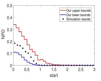
(a) Pd(v1)

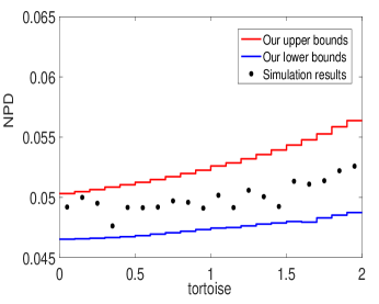
(b) Race(v2)

(c) RdWalk(v1)

(d) PdMB(v3)

Figure 8. NPD Bounds of Novel Examples

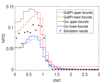
(a) Pd

(b) PdLD

(c) PdBeta(v1)

(d) PdBeta(v2)

Figure 9. NPD Bounds of Comparison

• The red and the blue lines mark the upper and lower bounds of our results; the black bold stars mark the simulation results; the brown and green dotted lines mark the upper and lower bounds generated by GuBPI (we denote by $-0.1$ the infinity bounds).

NPD - Comparision with GuBPI (Beutner et al., 2022). Since the parameters used in GuBPI and our approach are completely different, it is infeasible to compare the two approaches directly. Instead, we choose the parameters to our algorithms that can achieve at least comparable results with GuBPI. The main parameters are shown in Table 2 and we set the partition number $m=60$. We consider the Pedestrian example “Pd” from (Beutner et al., 2022) (see also Section 3.1), and its variants. More concretely, we enlarged the standard deviation of the observed normal distribution to be $5$ for all other $6$ examples whose prefix name are “Pd”; for the four “PdBeta” examples, we also add different beta distributions in the loop bodies. The last example is from (Gehr et al., 2016). We report the results in Table 2 whose layout is similar to Table 1 except that the column “#” displays whether or not the bounds are trivial, i.e., $[0,\infty]$. We also compare our results with GuBPI’s and simulation results ($10^{6}$ samples per case), and show part of the comparison in Fig. 9, see Appendix D for other figures. Our runtime is up to 6 times faster than GuBPI while we can still obtain tighter or comparable bounds for all examples. Specifically, for the first example “Pd”, our upper bounds are a bit higher than GuBPI’s when the value of $start$ falls into $[0,0.7]$ (which is not suprising as the deviation of the normal distribution in this example is quite small, i.e., $0.1$, and our approach constructs over-approximation constraints while GuPBI uses recursion unrolling to search for the feasible space exhaustively), but our lower bounds are greater than GuBPI’s, and our NPD bounds are tighter in the following. For all $6$ variants of “Pd” where the deviation of the normal distrbution is enlarged, our NPD bounds are tighter than GuBPI’s, in particular, our upper bounds are much lower than GuBPI’s. For the four “PdBeta” examples, we also found that GuBPI produced zero-valued unnormalized lower bounds, thus its results w.r.t. NPD are trivial, i.e., $[0,\infty]$. However, we can still produce non-trivial results and our runtime is at least 2 times faster than GuBPI.

Table 2. Comparison with GuBPI

Benchmark	Our Tool				GuBPI
	Parameters	Solver	Time (s)	#	Time (s)	#
Pd	$d=10$, $pos,dis\in[0,5]$	SDP	$3176.685$	$\bullet$	$5266.063$	$\bullet$
PdLD	$d=6$, $pos,dis\in[0,5]$	LP	$41.99$	$\bullet$	$648.151$	$\bullet$
PdBeta(v1)	$d=6$, $pos,dis\in[0,5]$	LP	$99.86$	$\bullet$	$645.055$	$\circ$
PdBeta(v2)	$d=6$, $pos,dis\in[0,5]$	LP	$228.43$	$\bullet$	$653.237$	$\circ$
PdBeta(v3)	$d=6$, $pos,dis\in[0,5]$	LP	$101.36$	$\bullet$	$657.645$	$\circ$
PdBeta(v4)	$d=6$, $pos,dis\in[0,5]$	LP	$208.86$	$\bullet$	$686.207$	$\circ$
PdMB(v5)	$d=6$, $pos,dis\in[0,5]$	LP	$88.41$	$\bullet$	$391.772$	$\bullet$
Para-recur	$d=8$, $p\in[0,1]$	LP	$36.61$	$\bullet$	$253.728$	$\bullet$

• $\circ$ marks the trivial bound $[0,\infty]$, while $\bullet$ marks the non-trivial ones.

Path Probability Estimation. We consider five recursive examples in (Beutner et al., 2022), which were also cited from the PSI repository (Gehr et al., 2016). Since all five examples are non-paramteric and with unbounded numbers of loop iterations, PSI cannot handle them correctly as mentioned in (Beutner et al., 2022). We estimated the path probability of certain events, i.e., queries over program variables, and report the results in Table 3. For the first three examples, we obtained tighter lower bounds than GuBPI and same upper bounds, while our runtime is at least 2 times faster than GuBPI. Moreover, we found a potential error of GuBPI. That is, the fourth example “cav-ex-5" in Table 3 is an AST program with no scores, which means its normalizing constant should be exactly one. However, the upper bound of the normailising constant obtained by GuBPI is smaller than $1$ (i.e., $0.6981$). A stochastic simulation using $10^{6}$ samples yielded the results that fall within our bounds but violate those computed by GuBPI. Thus, GuBPI possibly omitted some valid program runs of this example and produces wrong results. All our results match the simulation results ($10^{6}$ samples per case).

Table 3. Results for Path Probability Estimation

Benchmark	Query	Our Tool			GuBPI		Simul
		Parameters	Time (s)	Bounds	Time (s)	Bounds
cav-ex-7	Q1	$6,[0,30],[0,4]$	$15.062$	$[0.9698,1.0000]$	$38.834$	$[0.7381,1.0000]$	$0.9938$
	Q2	$6,[0,40],[0,4]$	$16.321$	$[0.9985,1.0000]$	$37.651$	$[0.7381,1.0000]$	$0.9993$
AddUni(L)	Q1	$6,[0,10],[0,1]$	$8.85$	$[0.9940,1.0000]$	$21.064$	$[0.9375,1.0000]$	$0.9991$
	Q2	$6,[0,15],[0,1]$	$8.80$	$[0.9995,1.0000]$	$14.941$	$[0.9375,1.0000]$	$0.9999$
RdBox	Q1	$4,[-0.8,0.8],[0,10]$	$25.87$	$[0.9801,1.0000]$	$173.535$	$[0.9462,1.0000]$	$0.9999$
cav-ex-5 *	Q1	$6,[20,\infty],[0,10]$	$33.17$	$[0.8123,0.9707]$	$229.623$	$[0.5768,0.6374]$	$0.9098$
	Q2	$6,[20,\infty],[0,20]$	$54.373$	$[0.8970,1.0000]$	$224.504$	$[0.5768,0.6375]$	$0.9645$
GWalk **	Q1	$8,[1,\infty],[0,0.1]$	$7.255$	$[0.0023,0.0023]$	$33.246$	$[0.0023,0.0024]$	$0.0023$
	Q2	$8,[1,\infty],[0,0.2]$	$8.197$	$[0.0025,0.0025]$	$31.728$	$[0.0025,0.0025]$	$0.0025$

• GuBPI’s result contradicts ours, and we found GuBPI produces wrong results for this example.

• As we care about path probabilities, we compared bounds of unnormalized distributions for this example (the NPD can be derived in the same manner above).

7. Related Works

Below we compare our results with the most related work in the literature.

Static analysis in Bayesian probabilistic programming.

There are a lot of works on NPD inference for probabilistic programs, such as $(\lambda)$PSI (Gehr et al., 2016, 2020), AQUA (Huang et al., 2021), Hakaru (Narayanan et al., 2016) and SPPL (Saad et al., 2021). However, these methods are restricted to specific kinds of programs, e.g., programs with closed-form solutions to NPD or without continuous distributions, and none of them can handle probabilistic programs with unbounded while-loops/recursion. As far as we know, the most revelant work on static analysis of posterior distribution over unbounded loops/recursion is the approach (Beutner et al., 2022) that infers the bounds for posterior distributions by recursion unrolling and bounding the non-termination case via the widening operator of abstract interpretation. By unrolling recursion to arbitrary depth, this approach can achieve high precision on the derive bounds. However, a major drawback of this approach is that the recursion unrolling may cause path explosion. Our approach circumvents the path explosion problem by constraint solving. Another major drawback is that this approach cannot handle score-recursive programs as simply applying the approach to score-recursive programs leads to the trivial bound $[0,\infty]$, and we address this issue by a novel OST variant.

MCMC and variational inference.

As mentioned previously, statistical approaches such as MCMC (Rubinstein and Kroese, 2016; Gamerman and Lopes, 2006) and variational inference (Blei et al., 2017) cannot provide formal guarantee on the bounds for posterior distributions in a finite time limit. In contrast, our approach has formal guarantee on the derived bounds.

Static analysis of probabilistic programs.

In recent years, there have been an abundance of works on static analysis of probabilistic programs. Most of them address fundamental aspects such as termination (Chakarov and Sankaranarayanan, 2013b; Chatterjee et al., 2016b; Fu and Chatterjee, 2019), sensitivity (Barthe et al., 2018; Wang et al., 2020), expectation (Ngo et al., 2018; Wang et al., 2019), tail bounds (Kura et al., 2019; Wang et al., 2021a; Wang, 2022), assertion probability (Sankaranarayanan et al., 2013; Wang et al., 2021b), etc. Compared with these results, we have:

• Our work focuses on normalized posterior distribution in Bayesian probabilistic programming, and hence is an orthogonal objective.

• Our algorithm follows the previous works on the synthesis of polynomial templates (Chakarov and Sankaranarayanan, 2013b; Wang et al., 2019; Chatterjee et al., 2018, 2016a), but we have a truncation operation to increase the accuracy which to our best knowledge is novel.

• Our approach extends the classical OST as the previous works (Wang et al., 2019, 2021a) do, but we consider a multiplicative variant, while the work  (Wang et al., 2019) considers only an additive variant, and the work (Wang et al., 2021a) considers a general extension through the uniform integrability condition and an implementation via polynomial functions, but does not have a detailed treatment for a multiplicative variant.

A very recent work (Batz et al., 2023) considers the synthesis of piecewise bounds for probabilistic programs. We focus on non-piecewise polynomial bounds and hence is orthognal. A promising future direction would be also to consider piecewise bounds in the NPD problem.

8. Conclusion

In this work, we considered the formal analysis of normalized posterior distribution in Bayesian probabilistic programming. Our contribution is a novel template-based approach that circumvents the the path explosion problem from loop/recursion unrolling and addresses score-recursive programs via a novel variant of Optional Stopping Theorem. A future direction would be to investigate whether our approach can be further improved by piecewise polynomials.

Appendix A Supplementary Material for Section 2

A.1. Basics of Probability Theory

A measurable space is a pair $(U,\Sigma_{U})$, where $U$ is a nonempty set and $\Sigma_{U}$ is a $\sigma$-algebra on $U$, i.e., a family of subsets of $U$ such that $\Sigma_{U}\subseteq\mathcal{P}(U)$ contains $\emptyset$ and is closed under complementation and countable union. Elements of $\Sigma_{U}$ are called measurable sets. A function $f$ from a measurable space $(U_{1},\Sigma_{U_{1}})$ to another measurable space $(U_{2},\Sigma_{U_{2}})$ is measurable if $f^{-1}(A)\in\Sigma_{U_{1}}$ for all $A\in\Sigma_{U_{2}}$.

A measure $\mu$ on a measurable space $(U,\Sigma_{U})$ is a mapping from $\Sigma_{U}$ to $[0,\infty]$ such that (i) $\mu(\emptyset)=0$ and (ii) $\mu$ is countably additive: for every pairwise-disjoint set sequence $\{A_{n}\}_{n\in\mathbb{N}}$ in $\Sigma_{U}$, it holds that $\mu(\bigcup_{n\in\mathbb{N}}A_{n})=\sum_{n\in\mathbb{N}}\mu(A_{n})$. We call the triple $(U,\Sigma_{U},\mu)$ a measure space. If $\mu(U)=1$, we call $\mu$ a probability measure, and $(U,\Sigma_{U},\mu)$ a probability space. The Lebesgue measure $\lambda$ is the unique measure on $(\mathbb{R},\Sigma_{\mathbb{R}})$ satisfying $\lambda([a,b))=b-a$ for all valid intervals $[a,b)$ in $\Sigma_{\mathbb{R}}$. For each $n\in\mathbb{N}$, we have a measurable space $(\mathbb{R}^{n},\Sigma_{\mathbb{R}^{n}})$ and a unique product measure $\lambda_{n}$ on $\mathbb{R}^{n}$ satisfying $\lambda_{n}(\prod_{i=1}^{n}A_{i})=\prod_{i=1}^{n}\lambda(A_{i})$ for all $A_{i}\in\Sigma_{\mathbb{R}}$.

The Lebesgue integral operator $\int$ is a partial operator that maps a measure $\mu$ on $(U,\Sigma_{U})$ and a real-valued function $f$ on the same space $(U,\Sigma_{U})$ to a real number or infinity, which is denoted by $\int f\mathrm{d}\mu$ or $\int f(x)\mu(\mathrm{d}x)$. The detailed definition of Lebesgue integral is somewhat technical, see (Rankin, 1968; Rudin et al., 1976) for more details. Given a measurable set $A\in\Sigma_{U}$, the integral of $f$ over $A$ is defined by $\int_{A}f(x)\mu(\mathrm{d}x):=\int f(x)\cdot[x\in A]\mu(\mathrm{d}x)$ where $[-]$ is the Iverson bracket such that $[\phi]=1$ if $\phi$ is true, and $0$ otherwise. If $\mu$ is a probability measure, then we call the integral as the expectation of $f$, denoted by $\mathbb{E}_{x\sim\mu;A}\left[{f}\right]$, or $\mathbb{E}[f]$ when the scope is clear from the context.

For a measure $v$ on $(U,\Sigma_{U})$, a measurable function $f:U\to\mathbb{R}_{\geq 0}$ is the density of $v$ with respect to $\mu$ if $v(A)=\int f(x)\cdot[x\in A]\mu(\mathrm{d}x)$ for all measurable $A\in\Sigma_{U}$, and $\mu$ is called the reference measure (most often $\mu$ is the Lebesgue measure). Common families of probability distributions on the reals, e.g., uniform, normal distributions, are measures on $(\mathbb{R},\Sigma_{\mathbb{R}})$. Most often these are defined in terms of probability density functions with respect to the Lebesgue measure. That is, for each $\mu_{D}$ there is a measurable function $\text{pdf}_{D}:\mathbb{R}\to\mathbb{R}_{\geq 0}$ that determines it: $\mu_{D}(A):=\int_{A}\text{pdf}_{D}(\mathrm{d}\lambda)$. As we will see, density functions such as $\text{pdf}_{D}$ play an important role in Bayesian inference.

Given a probability space $(\Omega,\mathcal{F},\mathbb{P})$, a random variable is an $\mathcal{F}$-measurable function $X:\Omega\rightarrow\mathbb{R}\cup\{+\infty,-\infty\}$. The expectation of a random variable $X$, denoted by $\mathbb{E}(X)$, is the Lebesgue integral of $X$ w.r.t. $\mathbb{P}$, i.e., $\int X\,\mathrm{d}\mathbb{P}$. A filtration of $(\Omega,\mathcal{F},\mathbb{P})$ is an infinite sequence $\{\mathcal{F}_{n}\}_{n=0}^{\infty}$ such that for every $n\geq 0$, the triple $(\Omega,\mathcal{F}_{n},\mathbb{P})$ is a probability space and $\mathcal{F}_{n}\subseteq\mathcal{F}_{n+1}\subseteq\mathcal{F}$. A stopping time w.r.t. $\{\mathcal{F}_{n}\}_{n=0}^{\infty}$ is a random variable $T:\Omega\rightarrow\mathbb{N}\cup\{0,\infty\}$ such that for every $n\geq 0$, the event {$T\leq n$} is in $\mathcal{F}_{n}$.

A discrete-time stochastic process is a sequence $\Gamma=\{X_{n}\}_{n=0}^{\infty}$ of random variables in $(\Omega,\mathcal{F},\mathbb{P})$. The process $\Gamma$ is adapted to a filtration $\{\mathcal{F}_{n}\}_{n=0}^{\infty}$, if for all $n\geq 0$, $X_{n}$ is a random variable in $(\Omega,\mathcal{F}_{n},\mathbb{P})$. A discrete-time stochastic process $\Gamma=\{X_{n}\}_{n=0}^{\infty}$ adapted to a filtration $\{\mathcal{F}_{n}\}_{n=0}^{\infty}$ is a martingale (resp. supermartingale, submartingale) if for all $n\geq 0$, $\mathbb{E}(|X_{n}|)<\infty$ and it holds almost surely (i.e., with probability $1$) that ${\mathbb{E}}{\left[{X_{n+1}}\mid{\mathcal{F}_{n}}\right]}=X_{n}$ (resp. ${\mathbb{E}}{\left[{X_{n+1}}\mid{\mathcal{F}_{n}}\right]}\leq X_{n}$, ${\mathbb{E}}{\left[{X_{n+1}}\mid{\mathcal{F}_{n}}\right]}\geq X_{n}$). See (Williams, 1991) for details. Applying martingales to qualitative and quantitative analysis of probabilistic programs is a well-studied technique (Chakarov and Sankaranarayanan, 2013a; Chatterjee et al., 2016a, 2017).

A.2. Details for WPTS Semantics

We denote by $\Lambda$ the set of all states, by $\Delta$ the set of all weighted states, and by $\Sigma_{\Delta}$ the product $\sigma$-algebra (on $\Delta$) among the discrete $\sigma$-algebra $(L,2^{L})$ for locations, the $\sigma$-algebra $\Sigma_{\mathbb{R}^{|V_{\mathrm{p}}|}}$ for program valuations, and the $\sigma$-algebra $\Sigma_{\mathbb{R}}$ for the multiplicative likelihood weight. We define $\Sigma^{n}_{\Delta}$ (for $n\geq 1$) as the set $\{A_{1}\times\dots\times A_{n}\mid\forall 1\leq i\leq n.(A_{i}\in\Sigma_{\Delta})\}$, and $\Delta^{\infty}$ as the set of all infinite sequences of weighted states.

The probability space for the WPTS $\Pi$ is defined such that its sample space is the set of all program runs, its $\sigma$-algebra is generated by the countable union $\bigcup_{n\geq 1}\{B\times\Delta^{\infty}\mid B\in\Sigma^{n}_{\Delta}\}$), and its probability measure $\mathbb{P}$ is the unique one such that (i) $\mathbb{P}(A\times\Lambda^{\infty})=\mu_{\mathrm{init}}(\{\mathbf{v}\mid(\ell_{\mathrm{init}},\mathbf{v},1)\in A\})$ for all $A\in\Sigma_{\Delta}$, and (ii) $\mathbb{P}(A\times B\times\Delta^{\infty})$ (for every $A\in\Sigma_{\Delta},B\in\Sigma^{n}_{\Delta}$ ($n\geq 1$)) equals the probability w.r.t the sampling of $\mu_{\mathrm{init}}$ (for the initial program valuation) and $\mathcal{D}$ (for a sampling valuation in each step until the $(n+1)$-th step) that a program run $\{\Theta_{n}\}_{n\geq 0}$ is subject to $\Theta_{0}\in A$ and $(\Theta_{1},\dots,\Theta_{n+1})\in B$. For each program valuation $\mathbf{v}$, we denote by $\mathbb{P}_{\mathbf{v}}$ the probability measure of $\Pi$ when the initial distribution is changed to the Dirac distribution at $\mathbf{v}$.

A.3. Sampling-based Semantics

We recall one prominent semantics in the literature, i.e., the sampling-based semantics (Borgström et al., 2016; Staton et al., 2016). We show that the transition-based semantics in our work is equivalent to the widely-used sampling-based semantics in Bayesian statistical probabilistic programming.

The sampling-based semantics by Borgström et al. (Borgström et al., 2016) interprets a probabilistic program as a deterministic program parameterized by a sequence of random draws sampled during the execution of the program.

A sampling trace is a finite sequence $\boldsymbol{t}=\langle r_{1},\dots,r_{n}\rangle$ of real numbers, and we define $\mathcal{T}:=\bigcup_{n\in\mathbb{N}}\mathbb{R}^{n}$ as the set of all sampling traces. Given a probabilistic program $P$, a configuration $\sigma$ under the semantics is a tuple $\langle\mathbf{v},S,w,\boldsymbol{t}\rangle$ where $\mathbf{v}\in\mbox{\sl Val}_{V_{\mathrm{p}}}$ , $S$ is the statement to be executed, $w\in[0,\infty)$ is the global weight variable whose value expresses how well the current computation matches the observations, and $\boldsymbol{t}$ is a sampling trace. We denote by $\Sigma$ the set of all configurations.

The semantics operates on the configurations, where an execution of the program is initialized with $\sigma_{0}=\langle\mathbf{v}_{0},P,1,\boldsymbol{t}\rangle$, and the termination configurations have the form of $\langle\_,\textbf{skip},\_,[]\rangle$, for which $\_$ is a “wildcard” character that matches everything and $[]$ is an empty set. Fig. 10 shows the corresponding one-step reduction relation $\to$ (note that $\Downarrow$ is the usual big-step semantics for deterministic Boolean and arithmetic expressions, so we omit it here).

Let $\to^{*}$ be the reflexive transitive closure of the one-step reduction $\to$ in Fig. 10. Given a probabilistic program $P$, we call a sampling trace $\boldsymbol{t}$ terminating if $\langle\mathbf{v},P,1,\boldsymbol{t}\rangle\to^{*}\langle\mathbf{v}^{\prime},\text{skip},w,[]\rangle$ for some valuations $\mathbf{v},\mathbf{v}^{\prime}\in\mbox{\sl Val}_{V_{\mathrm{p}}}$ and weight $w\in\mathbb{R}_{\geq 0}$, i.e., the program $P$ terminates under the samples drawn as in $\boldsymbol{t}$.

                        $\langle\mathbf{v},\textbf{skip},w,\boldsymbol{t}\rangle\to\langle\mathbf{v},\textbf{skip},w,\boldsymbol{t}\rangle$

                  $\mathbf{v}\vdash E\Downarrow r$     $\langle\mathbf{v},x:=E,w,\boldsymbol{t}\rangle\to\langle\mathbf{v}[x\mapsto r],\textbf{skip},w,\boldsymbol{t}\rangle$

                  $\mathbf{v}\vdash B\Downarrow b$, $b=\textbf{true}$     $\langle\mathbf{v},\textbf{if}\,B\,\textbf{then}\,S_{1}\ \textbf{else}\ S_{2}\ \textbf{fi},w,\boldsymbol{t}\rangle\to\langle\mathbf{v},S_{1},w,\boldsymbol{t}\rangle$

                 $\mathbf{v}\vdash B\Downarrow b$, $b=\textbf{false}$     $\langle\mathbf{v},\textbf{if}\,B\,\textbf{then}\,S_{1}\ \textbf{else}\ S_{2}\ \textbf{fi},w,\boldsymbol{t}\rangle\to\langle\mathbf{v},S_{2},w,\boldsymbol{t}\rangle$

                        $w^{\prime}=\text{pdf}_{D}(r)\geq 0$     $\langle\mathbf{v},x:=\textbf{sample}\ D,w,r::\boldsymbol{t}\rangle\rightarrow\langle\mathbf{v}[x\mapsto r],\textbf{skip},w\cdot w^{\prime},\boldsymbol{t}\rangle$

                           $\mathbf{v}\vdash B\Downarrow b$, $b=\textbf{true}$     $\langle\mathbf{v},\textbf{while}\ B\ \textbf{do}\ S\ \textbf{od},w,\boldsymbol{t}\rangle\rightarrow\langle\mathbf{v},S;\textbf{while}\ B\ \textbf{do}\ S\ \textbf{od},w,\boldsymbol{t}\rangle$

                $\mathbf{v}\vdash B\Downarrow b$, $b=\textbf{false}$     $\langle\mathbf{v},\textbf{while}\ B\ \textbf{do}\ S\ \textbf{od},w,\boldsymbol{t}\rangle\rightarrow\langle\mathbf{v},\textbf{skip},w,\boldsymbol{t}\rangle$

                 $w^{\prime}=\text{pdf}_{D}(x)\geq 0$     $\langle\mathbf{v},\textbf{observe}(x,D),w,\boldsymbol{t}\rangle\rightarrow\langle\mathbf{v},\textbf{skip},w\cdot w^{\prime},\boldsymbol{t}\rangle$

  $\langle\mathbf{v},S_{1},w,\boldsymbol{t}\rangle\to\langle\mathbf{v}^{\prime},S^{\prime}_{1},w^{\prime},\boldsymbol{t}^{\prime}\rangle$, $S^{\prime}_{1}\neq\textbf{skip}$       $\langle\mathbf{v},S_{1};S_{2},w,\boldsymbol{t}\rangle\rightarrow\langle\mathbf{v}^{\prime},S^{\prime}_{1};S_{2},w^{\prime},\boldsymbol{t}^{\prime}\rangle$

  $\langle\mathbf{v},S_{1},w,\boldsymbol{t}\rangle\to\langle\mathbf{v}^{\prime},S^{\prime}_{1},w^{\prime},\boldsymbol{t}^{\prime}\rangle$, $S^{\prime}_{1}=\textbf{skip}$         $\langle\mathbf{v},S_{1};S_{2},w,\boldsymbol{t}\rangle\rightarrow\langle\mathbf{v}^{\prime},S_{2},w^{\prime},\boldsymbol{t}^{\prime}\rangle$

                           $\langle\mathbf{v},\textbf{return}\ x,w,\boldsymbol{t}\rangle\rightarrow\langle\mathbf{v},\textbf{skip},w,t\rangle$

Figure 10. One-step reduction for probabilistic programs.

Below we define the notion of posterior distributions by the sampling-based semantics. From the one-step reduction rules (in Fig. 10), we can reason about the global behavior of probabilistic programs in terms of the sampling traces they produce. That is, given a probabilistic program $P$, and a terminating trace $\boldsymbol{t}$ such that $\langle\mathbf{v},P,1,\boldsymbol{t}\rangle\to^{*}\langle\mathbf{v}^{\prime},\text{skip},w,[]\rangle$ for valuations $\mathbf{v},\mathbf{v}^{\prime}\in\mbox{\sl Val}_{V_{\mathrm{p}}}$ and weight $w\in\mathbb{R}_{\geq 0}$, we define the value function $\mathsf{val}_{P}$ and the weight function $\mathsf{wt}_{P}$ as follows:

(4) $$\mathsf{val}_{P}(\mathbf{v},\boldsymbol{t}) =\begin{cases}\mathbf{v}^{\prime}&\text{if }\langle\mathbf{v},P,1,\boldsymbol{t}\rangle\to^{*}\langle\mathbf{v}^{\prime},\text{skip},w,[]\rangle\\ \text{unspecified}&\text{otherwise},\end{cases}$$

(5) $$\mathsf{wt}_{P}(\mathbf{v},\boldsymbol{t}) =\begin{cases}w&\text{if }\langle\mathbf{v},P,1,\boldsymbol{t}\rangle\to^{*}\langle\mathbf{v}^{\prime},\text{skip},w,[]\rangle\\ 0&\text{otherwise}.\end{cases}$$

Moreover, we denote the return variable by $\mathsf{val}_{P,\mathit{ret}}(\mathbf{v},\boldsymbol{t})$, i.e.,  $\mathsf{val}_{P,\mathit{ret}}(\mathbf{v},\boldsymbol{t}):=\mathbf{v}^{\prime}[\mathit{ret}]$. We also consider the measure space $(\mathcal{T},\Sigma_{\mathcal{T}},\mu_{\mathcal{T}})$ where $\mathcal{T}=\bigcup_{n\in\mathbb{N}}\mathbb{R}^{n}$ (as mentioned previously), $\Sigma_{\mathcal{T}}:=\{\bigcup_{n\in\mathbb{N}}U_{n}\mid U_{n}\in\Sigma_{\mathbb{R}^{n}}\}$ and $\mu_{\mathcal{T}}(U):=\sum_{n\in\mathbb{N}}\lambda_{n}(U\cap\mathbb{R}^{n})$. By definition, the measure space $(\mathcal{T},\Sigma_{\mathcal{T}},\mu_{\mathcal{T}})$ specifies the probability values for sets of sampling traces.

Posterior Distributions.

Given a probabilistic program $P$, an initial program valuation $\mathbf{v}\in\mbox{\sl Val}_{V_{\mathrm{p}}}$ and a measurable set $U\in\Sigma_{\mathbb{R}}$, we define the set of terminating traces where the value of the return variable falls into $U$ as

$$\mathcal{T}_{P,\mathbf{v},U}:=\{\boldsymbol{t}\in\mathcal{T}\mid\langle\mathbf{v},P,1,\boldsymbol{t}\rangle\to^{*}\langle\mathbf{v}^{\prime},\text{skip},w,[]\rangle,\mathbf{v}^{\prime}[\mathit{ret}]\in U\}$$

and the set of all terminating traces as

$$\mathcal{T}_{P,\mathbf{v}}:=\{\boldsymbol{t}\in\mathcal{T}\mid\langle\mathbf{v},P,1,\boldsymbol{t}\rangle\to^{*}\langle\mathbf{v}^{\prime},\text{skip},w,[]\rangle\}.$$

Note that $\mathcal{T}_{P,\mathbf{v}}=\mathcal{T}_{P,\mathbf{v},\mathbb{R}}$. Therefore, we can define the unnormalised density w.r.t $P,\mathbf{v},U$ as

(6) $$\llbracket P\rrbracket_{\mathbf{v}}(U):=\int_{\mathcal{T}_{P,\mathbf{v},U}}\mathsf{wt}_{P}(\mathbf{v},\boldsymbol{t})\,\mu_{\mathcal{T}}(\mathrm{d}\boldsymbol{t}).$$

That is, the integral takes all traces $\boldsymbol{t}$ on which $P$ starts from $\mathbf{v}$ and evaluates to a value in $U$, weighting each $\boldsymbol{t}$ with the weight $\mathsf{wt}_{P}(\mathbf{v},\boldsymbol{t})$ of the corresponding execution. The normalising constant is thus defined by

(7) $$Z_{P,\mathbf{v}}:=\int_{\mathcal{T}_{P,\mathbf{v}}}\mathsf{wt}_{P}(\mathbf{v},\boldsymbol{t})\,\mu_{\mathcal{T}}(\mathrm{d}\boldsymbol{t}).$$

Therefore, the normalised posterior distribution is defined as $\mathsf{posterior}_{P}(\mathbf{v},U):=\frac{\llbracket P\rrbracket_{\mathbf{v}}(U)}{Z_{P,\mathbf{v}}}$.

We call a program $P$ integrable if its normalised constant is finite, i.e, $0<Z_{P,\mathbf{v}}<\infty$ for any $\mathbf{v}\in\mbox{\sl Val}_{V_{\mathrm{p}}}$. Given an integrable program, we are interested in deriving lower and upper bounds on the posterior distribution.

Definition A.1 (Interval Bounds).

Given an integrable probabilistic program $P$, a program valuation $\mathbf{v}\in\mbox{\sl Val}_{V_{\mathrm{p}}}$, and a measurable set $U\in\Sigma_{\mathbb{R}}$, we call $[l,u]$ an interval bound of $\mathsf{posterior}_{P}(\mathbf{v},U)$ if $l\leq\mathsf{posterior}_{P}(\mathbf{v},U)\leq u$ for two reals $0\leq l\leq u\leq 1$.

A.4. Equivalence between Posterior Distributions and Expected Weights

In this subsection, we introduce the equivalence between posterior distributions (in sample-based semantics) and expected weights (in transition-based semantics: WPTS).

Lemma A.2.

For all non-negative bounded measurable function $g:\mathbb{R}^{|V_{\mathrm{p}}|}\to\mathbb{R}$, and a program state $\Xi=(\ell,\mathbf{v})$, and a statement $P:=S_{1};S_{2}$, we have that

$$\int_{\mathcal{T}_{P,\mathbf{v}}}\mathsf{wt}_{P}(\mathbf{v},\boldsymbol{t})\cdot g(\mathsf{val}_{P}(\mathbf{v},\boldsymbol{t}))\,\mu_{\mathcal{T}}(\mathrm{d}\boldsymbol{t})$$

$${}=\int_{\mathcal{T}_{S_{1},\mathbf{v}}}\mathsf{wt}_{S_{1}}(\mathbf{v},\boldsymbol{t})\,\mu_{\mathcal{T}}(\mathrm{d}\boldsymbol{t})\Big{(}[\mathsf{val}_{S_{1}}(\mathbf{v},\boldsymbol{t})=\mathbf{v}^{\prime}]$$

$$\quad{}\cdot\int_{\mathcal{T}_{S_{2},\mathbf{v}^{\prime}}}\mathsf{wt}_{S_{2}}(\mathbf{v}^{\prime},\boldsymbol{t}^{\prime})\cdot g(\mathsf{val}_{S_{2}}(\mathbf{v}^{\prime},\boldsymbol{t}^{\prime}))\,\mu_{\mathcal{T}}(\mathrm{d}\boldsymbol{t}^{\prime})\Big{)}$$

Proposition A.3.

For all non-negative bounded measurable function $g:\mathbb{R}^{|V_{\mathrm{p}}|}\to\mathbb{R}$, a probabilistic program $P$ and an initial program state $\Xi=(\ell,\mathbf{v})\in\Lambda$, we have that

$$\mathbb{E}_{\mathbf{v}}\left[{\widehat{w}_{T}\cdot g(\widehat{\mathbf{v}}_{T})}\right]=\int_{\mathcal{T}_{P,\mathbf{v}}}\mathsf{wt}_{P}(\mathbf{v},\boldsymbol{t})\cdot g(\mathsf{val}_{P}(\mathbf{v},\boldsymbol{t}))\,\mu_{\mathcal{T}}(\mathrm{d}\boldsymbol{t}).$$

Proof.

We prove by induction on the structure of statements.

• Case $P\equiv``\textbf{skip}"$.

  $$\mathbb{E}_{\mathbf{v}}\left[{\widehat{w}_{T}\cdot g(\widehat{\mathbf{v}}_{T})}\right] = \int\widehat{w}_{T}(\omega)\cdot g(\widehat{\mathbf{v}}_{T}(\omega))\mathbb{P}_{\Xi}(\mathrm{d}\omega)$$

  $$= g(\mathbf{v})$$

  $$= \int_{\mathcal{T}_{P,\mathbf{v}}}[\boldsymbol{t}=[]]\cdot g(\mathbf{v})\,\mu_{\mathcal{T}}(\mathrm{d}\boldsymbol{t})$$

  $$= \int_{\mathcal{T}_{P,\mathbf{v}}}\mathsf{wt}_{P}(\mathbf{v},\boldsymbol{t})\cdot g(\mathsf{val}_{P}(\mathbf{v},\boldsymbol{t}))\,\mu_{\mathcal{T}}(\mathrm{d}\boldsymbol{t})$$

• Case $P\equiv``x:=E"$.

  $$\mathbb{E}_{\mathbf{v}}\left[{\widehat{w}_{T}\cdot g(\widehat{\mathbf{v}}_{T})}\right] = \int\widehat{w}_{T}(\omega)\cdot g(\widehat{\mathbf{v}}_{T}(\omega))\mathbb{P}_{\Xi}(\mathrm{d}\omega)$$

  $$= g(\mathbf{v}[x\mapsto\llbracket E\rrbracket(\mathbf{v})])$$

  $$= \int_{\mathcal{T}_{P,\mathbf{v}}}[\boldsymbol{t}=[]]\cdot g(\mathbf{v}[x\mapsto\llbracket E\rrbracket(\mathbf{v})])\,\mu_{\mathcal{T}}(\mathrm{d}\boldsymbol{t})$$

  $$= \int_{\mathcal{T}_{P,\mathbf{v}}}\mathsf{wt}_{P}(\mathbf{v},\boldsymbol{t})\cdot g(\mathsf{val}_{P}(\mathbf{v},\boldsymbol{t}))\,\mu_{\mathcal{T}}(\mathrm{d}\boldsymbol{t})$$

• Case $P\equiv``x:=\textbf{sample}\ D"$.

  $$\mathbb{E}_{\mathbf{v}}\left[{\widehat{w}_{T}\cdot g(\widehat{\mathbf{v}}_{T})}\right] = \int\widehat{w}_{T}(\omega)\cdot g(\widehat{\mathbf{v}}_{T}(\omega))\mathbb{P}_{\Xi}(\mathrm{d}\omega)$$

  $$= \int g(\mathbf{v}[x\mapsto r])\mu_{D}(\mathrm{d}r)$$

  $$= \int_{\mathcal{T}_{P,\mathbf{v}}}\mathsf{wt}_{P}(\mathbf{v},\boldsymbol{t})\cdot g(\mathsf{val}_{P}(\mathbf{v},\boldsymbol{t}))\,\mu_{\mathcal{T}}(\mathrm{d}\boldsymbol{t})$$

• Case $P\equiv``\textbf{observe}(x,D)"$.

  $$\mathbb{E}_{\mathbf{v}}\left[{\widehat{w}_{T}\cdot g(\widehat{\mathbf{v}}_{T})}\right] = \int\widehat{w}_{T}(\omega)\cdot g(\widehat{\mathbf{v}}_{T}(\omega))\mathbb{P}_{\Xi}(\mathrm{d}\omega)$$

  $$= W_{\ell}(\mathbf{v})\cdot g(\mathbf{v})$$

  $$= \int_{\mathcal{T}_{P,\mathbf{v}}}\mathsf{wt}_{P}(\mathbf{v},\boldsymbol{t})\cdot g(\mathsf{val}_{P}(\mathbf{v},\boldsymbol{t}))\,\mu_{\mathcal{T}}(\mathrm{d}\boldsymbol{t})$$

• Case $P\equiv``\textbf{return}\ x"$.

  $$\mathbb{E}_{\mathbf{v}}\left[{\widehat{w}_{T}\cdot g(\widehat{\mathbf{v}}_{T})}\right] = \int\widehat{w}_{T}(\omega)\cdot g(\widehat{\mathbf{v}}_{T}(\omega))\mathbb{P}_{\Xi}(\mathrm{d}\omega)$$

  $$= g(\mathbf{v})$$

  $$= \int_{\mathcal{T}_{P,\mathbf{v}}}[\boldsymbol{t}=[]]\cdot g(\mathbf{v})\,\mu_{\mathcal{T}}(\mathrm{d}\boldsymbol{t})$$

  $$= \int_{\mathcal{T}_{P,\mathbf{v}}}\mathsf{wt}_{P}(\mathbf{v},\boldsymbol{t})\cdot g(\mathsf{val}_{P}(\mathbf{v},\boldsymbol{t}))\,\mu_{\mathcal{T}}(\mathrm{d}\boldsymbol{t})$$

• Case $P\equiv``\textbf{if}\ B\ \textbf{then}\ S_{1}\ \textbf{else}\ S_{2}\ \textbf{fi}"$. Assume the next state corresponding to the then-branch (resp. else-branch) is $\Xi_{1}=(\ell_{1},\mathbf{v})$ (resp. $\Xi_{2}=(\ell_{2},\mathbf{v})$). Then we obtain that

  $$\mathbb{E}_{\mathbf{v}}\left[{\widehat{w}_{T}\cdot g(\widehat{\mathbf{v}}_{T})}\right] = [\llbracket B\rrbracket(\mathbf{v})=true]\cdot\mathbb{E}_{\mathbf{v}}\left[{\widehat{w}_{T}\cdot g(\widehat{\mathbf{v}}_{T})}\right]+[\llbracket B\rrbracket(\mathbf{v})=false]\cdot\mathbb{E}_{\mathbf{v}}\left[{\widehat{w}_{T}\cdot g(\widehat{\mathbf{v}}_{T})}\right]$$

  $$= [\llbracket B\rrbracket(\mathbf{v})=true]\cdot\int_{\mathcal{T}_{S_{1},\mathbf{v}}}\mathsf{wt}_{S_{1}}(\mathbf{v},\boldsymbol{t})\cdot g(\mathsf{val}_{S_{1}}(\mathbf{v},\boldsymbol{t}))\,\mu_{\mathcal{T}}(\mathrm{d}\boldsymbol{t})$$

  $$+[\llbracket B\rrbracket(\mathbf{v})=false]\cdot\int_{\mathcal{T}_{S_{2},\mathbf{v}}}\mathsf{wt}_{S_{2}}(\mathbf{v},\boldsymbol{t})\cdot g(\mathsf{val}_{S_{2}}(\mathbf{v},\boldsymbol{t}))\,\mu_{\mathcal{T}}(\mathrm{d}\boldsymbol{t})$$

  $$= \int_{\mathcal{T}_{P,\mathbf{v}}}\mathsf{wt}_{P}(\mathbf{v},\boldsymbol{t})\cdot g(\mathsf{val}_{P}(\mathbf{v},\boldsymbol{t}))\,\mu_{\mathcal{T}}(\mathrm{d}\boldsymbol{t})$$

• Case $P\equiv``S_{1};S_{2}"$.

  $$\mathbb{E}_{\mathbf{v}}\left[{\widehat{w}_{T}\cdot g(\widehat{\mathbf{v}}_{T})}\right] = \int\widehat{w}_{T}(\omega)\mathbb{P}_{\Xi}(\mathrm{d}\omega)\int[\omega_{T}=\Xi^{\prime}]\cdot\widehat{w}_{T}(\omega^{\prime})\cdot g(\widehat{\mathbf{v}}_{T}(\omega^{\prime}))\mathbb{P}_{\Xi^{\prime}}(\mathrm{d}\omega^{\prime})$$

  $$= \int\widehat{w}_{T}(\omega)\mathbb{P}_{\Xi}(\mathrm{d}\omega)\left([\omega_{T}=\Xi^{\prime}]\cdot\int\cdot\widehat{w}_{T}(\omega^{\prime})\cdot g(\widehat{\mathbf{v}}_{T}(\omega^{\prime}))\mathbb{P}_{\Xi^{\prime}}(\mathrm{d}\omega^{\prime})\right)$$

  $$= \int\widehat{w}_{T}(\omega)\mathbb{P}_{\Xi}(\mathrm{d}\omega)\left([\omega_{T}=\Xi^{\prime}]\cdot\int_{\mathcal{T}_{S_{2},\mathbf{v}^{\prime}}}\mathsf{wt}_{S_{2}}(\mathbf{v}^{\prime},\boldsymbol{t}^{\prime})\cdot g(\mathsf{val}_{S_{2}}(\mathbf{v}^{\prime},\boldsymbol{t}^{\prime}))\,\mu_{\mathcal{T}}(\mathrm{d}\boldsymbol{t}^{\prime})\right)$$

  $$= \int_{\mathcal{T}_{S_{1},\mathbf{v}}}\mathsf{wt}_{S_{1}}(\mathbf{v},\boldsymbol{t})\,\mu_{\mathcal{T}}(\mathrm{d}\boldsymbol{t})\Big{(}[\mathsf{val}_{S_{1}}(\mathbf{v},\boldsymbol{t})=\mathbf{v}^{\prime}]$$

  $$\cdot\int_{\mathcal{T}_{S_{2},\mathbf{v}^{\prime}}}\mathsf{wt}_{S_{2}}(\mathbf{v}^{\prime},\boldsymbol{t}^{\prime})\cdot g(\mathsf{val}_{S_{2}}(\mathbf{v}^{\prime},\boldsymbol{t}^{\prime}))\,\mu_{\mathcal{T}}(\mathrm{d}\boldsymbol{t}^{\prime})\Big{)}$$

  $$= \int_{\mathcal{T}_{P,\mathbf{v}}}\mathsf{wt}_{P}(\mathbf{v},\boldsymbol{t})\cdot g(\mathsf{val}_{P}(\mathbf{v},\boldsymbol{t}))\,\mu_{\mathcal{T}}(\mathrm{d}\boldsymbol{t})$$

  Here $\omega_{i}$ is the $i$-th element of the sequence $\omega=\{\Xi_{n}\}_{n\in\mathbb{N}}$, i.e., $\omega_{i}:=\Xi_{i}$. $\omega_{T}$ is the last element of $\omega$, and $\Xi^{\prime}=(\ell^{\prime},\mathbf{v}^{\prime})$. The third and fourth equalities follow from the induction hypothesis, and the last equality from Lemma A.2.

• Case $P\equiv``\textbf{while}\ B\ \textbf{do}\ S\ \textbf{od}"$. Assume the next state corresponding to the entry of the loop (resp. the exit of the loop) is $\Xi_{1}=(\ell_{1},\mathbf{v})$ (resp. $\Xi_{2}=(\ell_{2},\mathbf{v})$). Then we obtain that

  $$\mathbb{E}_{\mathbf{v}}\left[{\widehat{w}_{T}\cdot g(\widehat{\mathbf{v}}_{T})}\right] = [\llbracket B\rrbracket(\mathbf{v})=true]\cdot\mathbb{E}_{\Xi_{1}}\left[{\widehat{w}_{T}\cdot g(\widehat{\mathbf{v}}_{T})}\right]+[\llbracket B\rrbracket(\mathbf{v})=false]\cdot\mathbb{E}_{\Xi_{2}}\left[{\widehat{w}_{T}\cdot g(\widehat{\mathbf{v}}_{T})}\right]$$

  $$= [\llbracket B\rrbracket(\mathbf{v})=true]\cdot\int\widehat{w}_{T}(\omega)\cdot g(\widehat{\mathbf{v}}_{T})\mathbb{P}_{\Xi_{1}}(\mathrm{d}\omega)+[\llbracket B\rrbracket(\mathbf{v})=false]\cdot g(\mathbf{v})$$

  $$= [\llbracket B\rrbracket(\mathbf{v})=true]\cdot\int_{\mathcal{T}_{S;P,\mathbf{v}}}\mathsf{wt}_{S;P}(\mathbf{v},\boldsymbol{t})\cdot g(\mathsf{val}_{S;P}(\mathbf{v},\boldsymbol{t}))\,\mu_{\mathcal{T}}(\mathrm{d}\boldsymbol{t})$$

  $$+[\llbracket B\rrbracket(\mathbf{v})=false]\cdot\int_{\mathcal{T}_{\textbf{skip},\mathbf{v}}}[\boldsymbol{t}=[]]\cdot g(\mathsf{val}_{\textbf{skip}}(\mathbf{v},\boldsymbol{t}))\,\mu_{\mathcal{T}}(\mathrm{d}\boldsymbol{t})$$

  $$= \int_{\mathcal{T}_{P,\mathbf{v}}}\mathsf{wt}_{P}(\mathbf{v},\boldsymbol{t})\cdot g(\mathsf{val}_{P}(\mathbf{v},\boldsymbol{t}))\,\mu_{\mathcal{T}}(\mathrm{d}\boldsymbol{t})$$

∎

Theorem A.4.

Given a probabilistic program $P$, an initial program state $\Xi=(\ell,\mathbf{v})\in\Lambda$ and a measurable set $U\in\Sigma_{\mathbb{R}}$, it holds that $\mathbb{E}_{\Xi}\left[{\widehat{w}_{T}\cdot[\widehat{\mathbf{v}}_{T}\in\mathcal{U}]}\right]=\llbracket P\rrbracket_{\mathbf{v}}(\mathcal{U})$. Moreover, the expected weight $\mathbb{E}_{\Xi}\left[{\widehat{w}_{T}}\right]$ is equivalent to the normalising constant $Z_{P}$.

Proof.

We instantiate Proposition A.3 with $g(x)=[x\in\mathcal{U}]$. For any initial program state $\Xi=(\ell,\mathbf{v})$, we have that

$$\mathbb{E}_{\mathbf{v}}\left[{\widehat{w}_{T}\cdot[\widehat{\mathbf{v}}_{T}\in\mathcal{U}]}\right] = \int_{\mathcal{T}_{P,\mathbf{v}}}\mathsf{wt}_{P}(\mathbf{v},\boldsymbol{t})\cdot[\mathsf{val}_{P}(\mathbf{v},\boldsymbol{t})\in\mathcal{U}]\,\mu_{\mathcal{T}}(\mathrm{d}\boldsymbol{t})$$

$$= \int_{\mathcal{T}_{P,\mathbf{v},U}}\mathsf{wt}_{P}(\mathbf{v},\boldsymbol{t})\,\mu_{\mathcal{T}}(\mathrm{d}\boldsymbol{t})$$

$$= \llbracket P\rrbracket_{\mathbf{v}}(\mathcal{U})$$

We prove $\mathbb{E}_{\mathbf{v}}\left[{\widehat{w}_{T}}\right]=Z_{P}$ by setting $\mathcal{U}=\mathbb{R}$. ∎

By Theorem A.4, we show the equivalence between posterior distributions under sampling-based semantics and expected weights under transition-based semantics. In the following, we will focus on developing approach es to infer interval bounds on expected weights.

A.5. Proof for Proposition 2.8

Proposition A.5.

Given a WPTS in the form of († ‣ 2.2), the interval-bound analysis of $Z_{\Pi}$ can be reduced to the interval-bound analysis of the expected weight $\llbracket\Pi\rrbracket_{\mathbf{v}}(\mathbb{R}^{|V_{\mathrm{p}}|})$ for all $\mathbf{v}\in\mathcal{V}$.

Proof.

Fix a WPTS $\Pi$ in the form of († ‣ 2.2). By Definition 2.7, the normalising constant $Z_{\Pi}=\llbracket\Pi\rrbracket(\mathbb{R}^{|V_{\mathrm{p}}|})=\int_{\mathcal{V}}\llbracket\Pi\rrbracket_{\mathbf{v}}(\mathbb{R}^{V_{\mathrm{p}}})\cdot\mu_{\mathrm{init}}(\mathrm{d}\mathbf{v})$ is the integral of the expected weight function $\llbracket\Pi\rrbracket_{\mathbf{v}}(\mathbb{R}^{|V_{\mathrm{p}}|})$ over the finite set $\mathcal{V}=\textsf{supp}\left({\mu_{\mathrm{init}}}\right)$. Assume there exist two integrable bound functions $Up,Lw$ such that $Lw(\mathbf{v})\leq\llbracket\Pi\rrbracket_{\mathbf{v}}(\mathbb{R}^{|V_{\mathrm{p}}|})\leq Up(\mathbf{v})$ for all $\mathbf{v}\in\mathcal{V}$. Then the interval bounds $l_{Z},u_{Z}$ for $Z_{\Pi}$ can be derived by the integrals of $Up,Lw$ over $\mathcal{V}$, that is,

$$l_{Z}:=\int_{\mathcal{V}}Lw(\mathbf{v})\cdot\mu_{\mathrm{init}}(\mathrm{d}\mathbf{v})\leq\llbracket\Pi\rrbracket(\mathbb{R}^{|V_{\mathrm{p}}|})=\int_{\mathcal{V}}\llbracket\Pi\rrbracket_{\mathbf{v}}(\mathbb{R}^{|V_{\mathrm{p}}|})\cdot\mu_{\mathrm{init}}(\mathrm{d}\mathbf{v})\leq\int_{\mathcal{V}}Up(\mathbf{v})\cdot\mu_{\mathrm{init}}(\mathrm{d}\mathbf{v})=:u_{Z}.$$

∎

Proposition A.6.

Given a WPTS in the form of († ‣ 2.2) and any measurable set $\mathcal{U}\subsetneqq\mathbb{R}^{|V_{\mathrm{p}}|}$, the interval-bound analysis of $\llbracket\Pi\rrbracket(\mathcal{U})$ can be reduced to the interval-bound analysis of the expected weight $\llbracket\Pi\rrbracket_{\mathbf{v}}(\mathbb{R}^{|V_{\mathrm{p}}|})$ for all $\mathbf{v}\in\mathcal{V}^{\prime}\subseteq\mathcal{V}$.

Proof.

Fix a WPTS $\Pi$ in the form of († ‣ 2.2) and a measurable set $\mathcal{U}\subsetneqq\mathbb{R}^{|V_{\mathrm{p}}|}$. By Definition 2.7, $\llbracket\Pi\rrbracket(\mathcal{U})=\int_{\mathcal{V}}\llbracket\Pi\rrbracket_{\mathbf{v}}(\mathcal{U})\cdot\mu_{\mathrm{init}}(\mathrm{d}\mathbf{v})$. By Definition 2.6, $\llbracket\Pi\rrbracket_{\mathbf{v}}(\mathcal{U})=\mathbb{E}_{\mathbf{v}}\left[{[\widehat{\mathbf{v}}_{T}\in\mathcal{U}]\cdot\widehat{w}_{T}}\right]$ for any initial program valuation $\mathbf{v}$. As $\widehat{\mathbf{v}}_{T}$ is the random (vector) variable of the program valuation at termination and $\mathcal{U}\neq\mathbb{R}^{|V_{\mathrm{p}}|}$, it is not possible to track the valuation of $\widehat{\mathbf{v}}_{T}$ for each program run starting from $\mathbf{v}$, which makes it challenging to compute interval bounds for $\llbracket\Pi\rrbracket_{\mathbf{v}}(\mathcal{U})$ directly. However, in practice, we only care about the posterior distribution that whether the return variable falls into some target sets of interest. That is, the set $\mathcal{U}$ is defined such that $[\widehat{\mathbf{v}}_{T}\in\mathcal{U}]=1$ iff $\widehat{\mathbf{v}}_{T}[ret]\in\mathcal{U}(ret)$ where $\mathcal{U}(ret)$ is the element in $\mathcal{U}$ that corresponds to the set w.r.t. the return variable. Below we distinguish the computation into two cases.

• If the value of $ret$ is determined once and unaffected by loop iterations, then $[\widehat{\mathbf{v}}_{T}[ret]\in\mathcal{U}(ret)]$ is equivalent to $[\mathbf{v}_{\mathrm{init}}[ret]\in\mathcal{U}(ret)]$. We can conclude that $\llbracket\Pi\rrbracket_{\mathbf{v}_{\mathrm{init}}}(\mathcal{U})=\\ \mathbb{E}_{\mathbf{v}_{\mathrm{init}}}\left[{[\widehat{\mathbf{v}}_{T}\in\mathcal{U}]\cdot\widehat{w}_{T}}\right]=\mathbb{E}_{\mathbf{v}_{\mathrm{init}}}\left[{\widehat{w}_{T}}\right]=\llbracket\Pi\rrbracket_{\mathbf{v}_{\mathrm{init}}}(\mathbb{R}^{|V_{\mathrm{p}}|})$ if $\mathbf{v}_{\mathrm{init}}[ret]\in\mathcal{U}(ret)$, and $0$ otherwise.

• If the value of $ret$ is affected during loop iterations, then we can construct a WPTS $\Pi_{\mathcal{U}}$ by adding a conditional branch of the form “if $\mathbf{v}_{T}\notin\mathcal{U}$ then score($0$) fi” immediately before the termination of $\Pi$. And we can prove that $\llbracket\Pi\rrbracket_{\mathbf{v}_{\mathrm{init}}}(\mathcal{U})$ is equivalent to $\llbracket\Pi_{\mathcal{U}}\rrbracket_{\mathbf{v}_{\mathrm{init}}}(\mathbb{R}^{|V_{\mathrm{p}}|})$ for all $\mathbf{v}_{\mathrm{init}}\in\mathcal{V}$.

The correctness of Case 1 above is straightforward to be proved, while the correctness of Case 2 follows from the proposition below. ∎

Proposition A.7.

Given a WPTS $\Pi$ in the form of († ‣ 2.2) and a measurable set $\mathcal{U}\subsetneqq\mathbb{R}^{|V_{\mathrm{p}}|}$, for any initial program valuation $\mathbf{v}_{\mathrm{init}}\in\mathcal{V}$, the expected weight $\llbracket\Pi\rrbracket_{\mathbf{v}_{\mathrm{init}}}(\mathcal{U})$ is equivalent to $\llbracket\Pi_{\mathcal{U}}\rrbracket_{\mathbf{v}_{\mathrm{init}}}(\mathbb{R}^{|V_{\mathrm{p}}|})$ where $\Pi_{\mathcal{U}}$ is constructed by the method described in Case 2 above.

Proof.

Fix a WPTS $\Pi$ in the form of († ‣ 2.2), a measurable set $\mathcal{U}\subsetneqq\mathbb{R}^{|V_{\mathrm{p}}|}$ and a new WPTS $\Pi_{\mathcal{U}}$ constructed by the method described in Case 2. Let the termination location of $\Pi$ be $\ell_{\mathrm{out}}$ and the termination location of $\Pi_{\mathcal{U}}$ be $\ell_{\mathrm{out}}^{\prime}$. Define a predicate $\Phi_{\mathcal{U}}$ over $V_{\mathrm{p}}$ such that $\mathcal{U}=\{\mathbf{v}\mid\mathbf{v}\models\Phi_{\mathcal{U}}\}$. Then $\Pi_{\mathcal{U}}$ has two additional transitions than $\Pi$, i.e., $\langle\ell_{\mathrm{out}},\Phi_{\mathcal{U}},F_{\top}\rangle$ with $F_{\top}:=\langle\ell_{\mathrm{out}}^{\prime},1,\mbox{\sl id},\overline{0}\rangle$ where id is the identity function and $\overline{0}$ is the constant function that always takes the value $0$, and $\langle\ell_{\mathrm{out}},\neg\Phi_{\mathcal{U}},F_{\bot}\rangle$ with $F_{\bot}:=\langle\ell_{\mathrm{out}}^{\prime},1,\mbox{\sl id},\overline{1}\rangle$ where $\overline{1}$ is the constant function that always takes the value $1$. Let the termination time of $\Pi$ be $T$ and the termination time of $\Pi_{\mathcal{U}}$ be $T^{\prime}$. Therefore, for the random variable of the multiplicative likelihood weight at termination, we have that $\widehat{w}_{T^{\prime}}=[\widehat{\mathbf{v}}_{T^{\prime}}\in\mathcal{U}]\cdot\widehat{w}_{T}+[\widehat{\mathbf{v}}_{T^{\prime}}\notin\mathcal{U}]\cdot 0$. By Definition 2.6,

$$\llbracket\Pi\rrbracket_{\mathbf{v}_{\mathrm{init}}}(\mathcal{U}) =\mathbb{E}_{\mathbf{v}_{\mathrm{init}}}\left[{[\widehat{\mathbf{v}}_{T}\in\mathcal{U}]\cdot\widehat{w}_{T}}\right]$$

$$=\mathbb{E}_{\mathbf{v}_{\mathrm{init}}}\left[{[\widehat{\mathbf{v}}_{T}\in\mathcal{U}]\cdot\widehat{w}_{T}+[\widehat{\mathbf{v}}_{T}\notin\mathcal{U}]\cdot 0}\right]$$

$$=\mathbb{E}_{\mathbf{v}_{\mathrm{init}}}\left[{[\widehat{\mathbf{v}}_{T^{\prime}}\in\mathcal{U}]\cdot\widehat{w}_{T}+[\widehat{\mathbf{v}}_{T^{\prime}}\notin\mathcal{U}]\cdot 0}\right]$$

$$=\mathbb{E}_{\mathbf{v}_{\mathrm{init}}}\left[{\widehat{w}_{T^{\prime}}}\right]$$

$$=\mathbb{E}_{\mathbf{v}_{\mathrm{init}}}\left[{[\widehat{\mathbf{v}}_{T^{\prime}}\in\mathbb{R}^{|V_{\mathrm{p}}|}]\cdot\widehat{w}_{T^{\prime}}}\right]$$

$$=\llbracket\Pi_{\mathcal{U}}\rrbracket_{\mathbf{v}_{\mathrm{init}}}(\mathbb{R}^{|V_{\mathrm{p}}|})$$

where the third equality is derived from the fact that $\widehat{\mathbf{v}}_{T^{\prime}}=\widehat{\mathbf{v}}_{T}$ and the fourth equality is obtained from the fact that $[\widehat{\mathbf{v}}_{T^{\prime}}\in\mathbb{R}^{|V_{\mathrm{p}}|}]\equiv 1$. ∎

Based on Proposition A.5 and Proposition A.6, in the following (Section 4) we develop approaches to obtain interval bounds for expected weights in the form $\llbracket\Pi\rrbracket_{\mathbf{v}}(\mathbb{R}^{|V_{\mathrm{p}}|})$ where $\mathbf{v}$ is an initial program valuation.

Appendix B Supplementary Material for Section 4

B.1. Basics of Fixed Point Theory

Given a partial order $\sqsubseteq$ on a set $K$ and a subset $K^{\prime}\subseteq K,$ an upper bound of $K^{\prime}$ is an element $u\in K$ that is no smaller than every element of $K^{\prime}$, i.e., $\forall k^{\prime}\in K^{\prime}.~{}k^{\prime}\sqsubseteq u.$ Similarly, a lower bound for $K^{\prime}$ is an element $l$ that is no greater than every element of $K^{\prime},$ i.e. $\forall k^{\prime}\in K^{\prime}.~{}l\sqsubseteq k^{\prime}.$ The supremum of $K^{\prime},$ denoted by $\bigsqcup K^{\prime}$, is an element $u^{*}\in K$ such that $u^{*}$ is an upper-bound of $K^{\prime}$ and for every upper bound $u$ of $K^{\prime},$ we have $u^{*}\sqsubseteq u.$ Similarly, the infimum $\bigsqcap K^{\prime}$ is a lower bound $l^{*}$ of $K^{\prime}$ such that for every lower-bound $l$ of $K^{\prime},$ we have $l\sqsubseteq l^{*}.$ We define $\bot\!:=\!\bigsqcap K$ and $\top\!:=\!\bigsqcup K.$ In general, suprema and infima may not exist.

A partial order $(K,\sqsubseteq)$ is called a complete lattice if every subset $K^{\prime}\subseteq K$ has a supremum and an infimum. Given a partial order $(K,\sqsubseteq)$, a function $f:K\to K$ is called monotone if for every $k_{1}\sqsubseteq k_{2}$ in $K$, we have $f(k_{1})\sqsubseteq f(k_{2}).$

Given a complete lattice $(K,\sqsubseteq),$ a function $f:K\to K$ is called continuous if for every increasing chain $k_{0}\sqsubseteq k_{1}\sqsubseteq\ldots$ in $K,$ we have $f(\bigsqcup\{k_{n}\}_{n=0}^{\infty})=\bigsqcup\{f(k_{n})\}_{n=0}^{\infty},$ and cocontinuous if for every decreasing chain $k_{0}\sqsupseteq k_{1}\sqsupseteq\ldots$ of elements of $K,$ we have $f(\bigsqcap\{k_{n}\}_{n=0}^{\infty})=\bigsqcap\{f(k_{n})\}_{n=0}^{\infty}.$

Given a complete lattice $(K,\sqsubseteq)$ and a function $f:K\to K,$ an element $k\in K$ is called a fixed-point if $f(k)=k.$ Moreover, $k$ is a pre fixed-point if $f(k)\sqsubseteq k$ and a post fixed-point if $k\sqsubseteq f(k)$. The least fixed-point of $f$, denoted by $\mathrm{lfp}f,$ is the fixed-point that is no greater than every fixed-point under $\sqsubseteq.$ Analogously, the greatest fixed-point of $f$, denoted by $\mathrm{gfp}f$, is the fixed-point that is no smaller than all fixed-points.

Theorem B.1 (Kleene (Sangiorgi, 2011)).

Let $(K,\sqsubseteq)$ be a complete lattice and $f:K\to K$ be an continuous function. Then, we have

$$\textstyle\mathrm{lfp}\ f={\textstyle\mathop{\bigsqcup}_{i\geq 0}}\left\{f^{(i)}(\bot)\right\}.$$

Analogously, if $f$ is cocontinuous, then we have

$$\textstyle\mathrm{gfp}\ f={\textstyle\mathop{\bigsqcap}_{i\geq 0}}\left\{f^{(i)}(\top)\right\}.$$

B.2. Proofs for Our Fixed-Point Approach

Theorem B.2.

The expected-weight function ew is the least fixed point of the expected-weight transformer ewt.

Proof.

Define the step-bounded weight random variable $\widehat{w}^{n}_{(\ell,\mathbf{v})}$ starting from any program state $\Xi=(\ell,\mathbf{v})$ for a step bound $n\in\mathbb{N}$ by

$$\widehat{w}^{n}_{(\ell,\mathbf{v})}(\omega)=\begin{cases}\widehat{w}_{(\ell,\mathbf{v})}(\omega)&\mbox{if $T(\omega)\leq n$}\\ 0&\mbox{otherwise}\end{cases}\enskip.$$

Since we always assume that the underlying WPTS is almost-surely terminating, it follows that the sequence of random variables $\{\widehat{w}^{n}\}_{n\in\mathbb{N}}$ converges non-decreasingly to $W$.

Given any program state $\Xi=(\ell,\mathbf{v})$ with a unique transition $\tau=\langle\ell,\phi_{\tau},f_{\tau}\rangle$ satisfying $\mathbf{v}\models\phi_{\tau}$, define the step-bounded expected-weight function $\mbox{\sl ew}^{n}$ by $\mbox{\sl ew}^{n}(\ell,\mathbf{v})=\mathbb{E}_{(\ell,\mathbf{v})}\left[{\widehat{w}^{n}}\right]$. Without loss of generality, we assume there is only one fork $f_{\tau}$ in this transition. Assume the next sampling valuation from $\Xi$ is $\mathbf{r}_{0}$ and the next program state is $\Xi^{\prime}=(\ell^{\prime},\mathbf{v}^{\prime})$, i.e., $\mathbf{v}^{\prime}=f_{\tau}(\mathbf{v},\mathbf{r}_{0})$. Following the symbols in Section 2, we denote the probability space of the WPTS $\Pi$ starting from $(\ell,\mathbf{v})$, i.e., the program runs starting from $\Xi=(\ell,\mathbf{v})$ as $(\Omega,\mathcal{F},\mathbb{P})_{\Xi}$. By Tonelli-Fubini Theorem, we have that for all $n\geq 0$,

$$\mbox{\sl ew}^{n+1}(\ell,\mathbf{v}) = \int\widehat{w}^{n+1}_{(\ell,\mathbf{v})}\,\mathrm{d}\mathbb{P}_{\Xi}$$

$$= \int\widehat{w}^{n+1}_{(\ell,\mathbf{v})}\,\mathrm{d}(\mathcal{D}_{\mathbf{r}_{0}}\times\mathbb{P}_{\Xi^{\prime}})$$

$$= \int\mbox{\sl wt}\cdot W^{n}_{(\ell^{\prime},\mathbf{v}^{\prime})}(\omega)\,\mathrm{d}(\mathcal{D}_{\mathbf{r}_{0}}\times\mathbb{P}_{\Xi^{\prime}})$$

$$= \int_{\mathbf{r}_{0}}\int_{\omega_{\Xi^{\prime}}}\mbox{\sl wt}\cdot W^{n}_{(\ell^{\prime},\mathbf{v}^{\prime})}(\omega)\,\mathrm{d}\mathbb{P}_{\Xi^{\prime}}\,\mathrm{d}\mathcal{D}_{\mathbf{r}_{0}}$$

$$= \int_{\mathbf{r}_{0}}\mbox{\sl wt}\cdot\left(\int_{\omega_{\Xi^{\prime}}}\widehat{w}^{n}_{(\ell^{\prime},\mathbf{v}^{\prime})}(\omega)\,\mathrm{d}\mathbb{P}_{\Xi^{\prime}}\right)\,\mathrm{d}\mathcal{D}_{\mathbf{r}_{0}}$$

$$= \int_{\mathbf{r}_{0}}\mbox{\sl wt}\cdot\mbox{\sl ew}^{n}(\ell^{\prime},\mathbf{v}^{\prime})\,\mathrm{d}\mathcal{D}_{\mathbf{r}_{0}}$$

$$= \mathbb{E}_{\mathbf{r}_{0}}\left[{\mbox{\sl wt}\cdot\mbox{\sl ew}^{n}(\ell^{\prime},\mathbf{v}^{\prime})}\right]$$

$$= \mbox{\sl ewt}(\mbox{\sl ew}^{n})(\ell,\mathbf{v})$$

By applying MCT to the both sides of the equality above, we have that

$$\mbox{\sl ew}(\ell,\mathbf{v})=\mbox{\sl ewt}(\mbox{\sl ew})(\ell,\mathbf{v}).$$

This shows that ew is a fixed point of ewt. Furthermore, given any fixed point $h$ of ewt, since (i) $\mbox{\sl ew}^{0}\leq h$ and (ii) $\mbox{\sl ew}^{n}\leq h$ implies $\mbox{\sl ew}^{n+1}=\mbox{\sl ewt}(\mbox{\sl ew}^{n})\leq\mbox{\sl ewt}(h)=h$, one can prove by a straightforward induction on $n$ that $\mbox{\sl ew}^{n}\leq h$ for all $n\geq 0$. It follows from $\mbox{\sl ew}=\lim\limits_{n\rightarrow\infty}\mbox{\sl ew}^{n}$ that ew is the least fixed point of ewt. ∎

In order to show the uniqueness of the fixed point, we first prove that ewt is both continuous and cocontinuous.

Proposition B.3.

If $M\in[0,\infty)$, then the expected-weight transformer $\mbox{\sl ewt}:\mathcal{K}_{M}\to\mathcal{K}_{M}$ is both continuous and cocontinous.

Proof.

We first prove that ewt is well-defined. Given an arbitrary $h\in\mathcal{K}_{M}$, for any $\Xi=(\ell,\mathbf{v})\in\Lambda$,

• When $\ell=\ell_{\mathrm{out}}$, $\mbox{\sl ewt}(h)(\ell,\mathbf{v})=1$.

• When $\ell\neq\ell_{\mathrm{out}}$, for a unique transition $\tau=\langle\ell,\phi_{\tau},f_{\tau},\ell^{\prime}\rangle$ such that $\mathbf{v}\models\phi_{\tau}$,

  $$\mbox{\sl ewt}(h)(\ell,\mathbf{v}) =\mathbb{E}_{\mathbf{r}}\left[{h(\ell^{\prime},f_{\tau}(\mathbf{v},\mathbf{r}))\cdot W(\ell,\mathbf{v})}\right]$$

  $$\leq M\cdot maxscore$$

  $$<\infty$$

where $maxscore$ is the maximum of $W$ given any state $\Xi$. As $W$ is a non-negative function, we can prove that $\mbox{\sl ewt}(h)(\ell,\mathbf{v})\geq 0$. Thus, ewt is well defined. Next, we prove that ewt is monotone. Given any two functions $h_{1},h_{2}\in\mathcal{K}_{M}$ such that $h_{1}\leq h_{2}$, by case analysis on $(\ell,\mathbf{v})$,

• If $\ell=\ell_{\mathrm{out}}$, $\mbox{\sl ewt}(h_{1})(\ell,\mathbf{v})=1=\mbox{\sl ewt}(h_{2})(\ell,\mathbf{v})$.

• If $\ell\neq\ell_{\mathrm{out}}$, given a unique transition $\tau=\langle\ell,\phi_{\tau},f_{\tau},\ell^{\prime}\rangle$ such that $\mathbf{v}\models\phi_{\tau}$,

  $$\mbox{\sl ewt}(h_{1})(\ell,\mathbf{v}) =\mathbb{E}_{\mathbf{r}}\left[{h_{1}(\ell^{\prime},f_{\tau}(\mathbf{v},\mathbf{r}))\cdot W(\ell,\mathbf{v})}\right]$$

  $$\leq\mathbb{E}_{\mathbf{r}}\left[{h_{2}(\ell^{\prime},f_{\tau}(\mathbf{v},\mathbf{r}))\cdot W(\ell,\mathbf{v})}\right]$$

  $$=\mbox{\sl ewt}(h_{2})(\ell,\mathbf{v})$$

Therefore, $\mbox{\sl ewt}(h_{1})\leq\mbox{\sl ewt}(h_{2})$, hence it is monotone. Then we prove upper continuity of ewt. Choose any increasing chain $h_{0}\sqsubseteq h_{1}\sqsubseteq h_{2}\sqsubseteq\cdots$ and do another case analysis on $(\ell,\mathbf{v})$:

• If $\ell=\ell_{\mathrm{out}}$, then

  $$\mbox{\sl ewt}(\mathop{\bigsqcup}\limits_{n\geq 0}\left\{h_{n}\right\})(\ell,\mathbf{v})=1=\mathop{\bigsqcup}\limits_{n\geq 0}\left\{\mbox{\sl ewt}(h_{n})\right\}(\ell,\mathbf{v}).$$

• Otherwise, for a unique transition $\tau=\langle\ell,\phi_{\tau},f_{\tau}\rangle$ such that $\mathbf{v}\models\phi_{\tau}$:

  $$\mbox{\sl ewt}(\mathop{\bigsqcup}\limits_{n\geq 0}\left\{h_{n}\right\})(\ell,\mathbf{v})$$

  $$= \mathbb{E}_{\mathbf{r}}\left[{\mbox{\sl wt}_{j}(\mathbf{v},\mathbf{r})\cdot(\mathop{\bigsqcup}\limits_{n\geq 0}\left\{h_{n}\right\})(\ell^{\prime},f_{\tau}(\mathbf{v},\mathbf{r}))}\right]$$

  $$= \mathbb{E}_{\mathbf{r}}\left[{\mathop{\text{sup}}\limits_{n\geq 0}\left\{h_{n}(\ell^{\prime},f_{\tau}(\mathbf{v},\mathbf{r}))\right\}}\right]$$

  $$= \mathbb{E}_{\mathbf{r}}\left[{\mathop{\text{lim}}\limits_{n\to\infty}\left\{h_{n}(\ell^{\prime},f_{\tau}(\mathbf{v},\mathbf{r}))\right\}}\right]$$

  $$\overset{\mathrm{MCT}}{=} \mathop{\text{lim}}\limits_{n\to\infty}\mathbb{E}_{\mathbf{r}}\left[{h_{n}(\ell^{\prime},f_{\tau}(\mathbf{v},\mathbf{r}))}\right]$$

  $$= \mathop{\text{lim}}\limits_{n\to\infty}\mbox{\sl ewt}(h_{n})(\ell,\mathbf{v})$$

  $$= \sup_{n\geq 0}\left\{\mbox{\sl ewt}(h_{n})(\ell,\mathbf{v})\right\}$$

  $$= \mathop{\bigsqcup}\limits_{n\geq 0}\left\{\mbox{\sl ewt}(h_{n})\right\}(\ell,\mathbf{v})$$

The “MCT” above denotes the monotone convergence theorem. A similar argument establishes cocontinuity for integrable $h_{0}$ and decreasing chains. ∎

Then the uniqueness follows from Theorem B.1.

Theorem 4.5. Let $\Pi$ be a non-score-recursive WPTS whose weights are bounded in $[-M,M]$ for a finite $M\geq 1$. Then the expected-weight function ew is the least fixed point of the expected-weight transformer ewt in the complete lattice $(\mathcal{K}_{M},\leq)$. Furthermore, if the WPTS $\Pi$ is AST, then the function ew is the unique fixed point of the higher-order function ewt in $(\mathcal{K}_{M},\leq)$ when $M\geq 1$.

Proof.

The proof follows similar arguments in (Wang et al., 2021b, Theorem 4.4). By Proposition B.3, we have that for every state $\Xi=(\ell,\mathbf{v})$,

• $\mathrm{lfp}\ \mbox{\sl ewt}(\ell,\mathbf{v})=\lim\limits_{n\rightarrow\infty}\mbox{\sl ewt}^{n}(\bot)(\ell,\mathbf{v})$, and

• $\mathrm{gfp}\ \mbox{\sl ewt}(\ell,\mathbf{v})=\lim\limits_{n\rightarrow\infty}\mbox{\sl ewt}^{n}(\top)(\ell,\mathbf{v})$.

By the definition of $\mbox{\sl ewt}_{M}^{n}$ and Proposition B.3, we have that

• $\mbox{\sl ewt}^{n}(\bot)(\ell,\mathbf{v})=\mathbb{E}_{\Xi}\left[{W\cdot[T\leq n]}\right]-M\cdot\mathbb{P}(T>n)$, and

• $\mbox{\sl ewt}^{n}(\top)(\ell,\mathbf{v})=\mathbb{E}_{\Xi}\left[{W\cdot[T\leq n]}\right]+M\cdot\mathbb{P}(T>n)$.

Recall that we assume the underlying PTS to be almost-surely terminating. Hence, $\lim\limits_{n\rightarrow\infty}\mathbb{P}(T>n)=\mathbb{P}(T=\infty)=0$. It follows that $\mathrm{lfp}\ \mbox{\sl ewt}(\ell,\mathbf{v})=\mathrm{gfp}\ \mbox{\sl ewt}(\ell,\mathbf{v})$, i.e., the fixed point is unique. ∎

B.3. Proof for the OST Variant

Theorem 4.8 (OST Variant) Let $\{X_{n}\}_{n=0}^{\infty}$ be a supermartingale adapted to a filtration $\mathcal{F}=\{\mathcal{F}_{n}\}_{n=0}^{\infty}$, and $\kappa$ be a stopping time w.r.t. the filtration $\mathcal{F}$. Then the following condition $(\mho)$ is sufficient to ensure that $\mathbb{E}\left(|X_{\kappa}|\right)<\infty$ and $\mathbb{E}\left(X_{\kappa}\right)\leq\mathbb{E}(X_{0})$:

• There exist integers $b_{1},b_{2}>0$ and real numbers $c_{1}>0,c_{2}>c_{3}>0$ such that (i) $\mathbb{P}(\kappa>n)\leq c_{1}\cdot e^{-c_{2}\cdot n}$ for sufficiently large $n\in\mathbb{N}$, and (ii) for all $n\in\mathbb{N}$, $\left|X_{n+1}-X_{n}\right|\leq b_{1}\cdot n^{b_{2}}\cdot e^{c_{3}\cdot n}$ holds almost surely.

Proof.

For every $n\in\mathbb{N}_{0}$,

$$\left|X_{\kappa\wedge n}\right| = \left|X_{0}+\sum_{k=0}^{\kappa\wedge n-1}\left(X_{k+1}-X_{k}\right)\right|$$

$$= \left|X_{0}+\sum_{k=0}^{\infty}\left(X_{k+1}-X_{k}\right)\cdot\mathbf{1}_{\kappa>k\wedge n>k}\right|$$

$$\leq \left|X_{0}\right|+\sum_{k=0}^{\infty}\left|\left(X_{k+1}-X_{k}\right)\cdot\mathbf{1}_{\kappa>k\wedge n>k}\right|$$

$$\leq \left|X_{0}\right|+\sum_{k=0}^{\infty}\left|\left(X_{k+1}-X_{k}\right)\cdot\mathbf{1}_{\kappa>k}\right|\enskip.$$

Then

$$\mathbb{E}\left(\left|X_{0}\right|+\sum_{k=0}^{\infty}\left|\left(X_{k+1}-X_{k}\right)\cdot\mathbf{1}_{\kappa>k}\right|\right)$$

$$=$$ (By Monotone Convergence Theorem)

$$\mathbb{E}\left(\left|X_{0}\right|\right)+\sum_{k=0}^{\infty}\mathbb{E}\left(\left|\left(X_{k+1}-X_{k}\right)\cdot\mathbf{1}_{\kappa>k}\right|\right)$$

$$= \mathbb{E}\left(\left|X_{0}\right|\right)+\sum_{k=0}^{\infty}\mathbb{E}\left(\left|X_{k+1}-X_{k}\right|\cdot\mathbf{1}_{\kappa>k}\right)$$

$$\leq \mathbb{E}\left(\left|X_{0}\right|\right)+\sum_{k=0}^{\infty}\mathbb{E}\left(\lambda\cdot k^{d}\cdot e^{c_{3}\cdot k}\cdot\mathbf{1}_{\kappa>k}\right)$$

$$= \mathbb{E}\left(\left|X_{0}\right|\right)+\sum_{k=0}^{\infty}\lambda\cdot k^{d}\cdot e^{c_{3}\cdot k}\cdot\mathbb{P}\left(\kappa>k\right)$$

$$\leq \mathbb{E}\left(\left|X_{0}\right|\right)+\sum_{k=0}^{\infty}\lambda\cdot k^{d}\cdot e^{c_{3}\cdot k}\cdot c_{1}\cdot e^{-c_{2}\cdot k}$$

$$= \mathbb{E}\left(\left|X_{0}\right|\right)+\lambda\cdot c_{1}\cdot\sum_{k=0}^{\infty}k^{d}\cdot e^{-(c_{2}-c_{3})\cdot k}$$

$$< \infty\enskip.$$

where the first inequality is obtained by Condition (ii), and the second inequality is derived from Condition (i).

Therefore, by Dominated Convergence Theorem and the fact that $X_{\kappa}=\lim\limits_{n\rightarrow\infty}X_{\kappa\wedge n}$ a.s.,

$$\mathbb{E}\left(X_{\kappa}\right)=\mathbb{E}\left(\lim\limits_{n\rightarrow\infty}X_{\kappa\wedge n}\right)=\lim\limits_{n\rightarrow\infty}\mathbb{E}\left(X_{\kappa\wedge n}\right)\enskip.$$

Finally, the result follows from properties for the stopped process $\{X_{\kappa\wedge n}\}_{n\in\mathbb{N}_{0}}$ that

$$\mathbb{E}\left(X_{\kappa}\right)\leq\mathbb{E}\left(X_{0}\right)\enskip.$$

∎

B.4. Proofs for Our OST-Based Approach

Theorem 4.9. [Upper Bounds on Expected Weights] Let $\Pi$ be a score-recursive WPTS that has the bounded update property. Suppose that there exist real numbers $c_{1}>0$ and $c_{2}>c_{3}>0$ such that

• $\mathbb{P}(\kappa>n)\leq c_{1}\cdot e^{-c_{2}\cdot n}$ for sufficiently large $n\in\mathbb{N}$, and

• for each score function wt in $\Pi$ we have $|\mbox{\sl wt}|\leq e^{c_{3}}$.

Then for any PUWF $h$ over $\Pi$, we have that $\llbracket\Pi\rrbracket_{\mathbf{v}_{\mathrm{init}}}(\mathbb{R}^{|V_{\mathrm{p}}|})\leq h(\ell_{\mathrm{init}},\mathbf{v}_{\mathrm{init}})$ for any initial state $(\ell_{\mathrm{init}},\mathbf{v}_{\mathrm{init}})$.

Proof.

Define the stochastic process $\{X_{n}\}_{n=0}^{\infty}$ as $X_{n}:=h(\ell_{n},\mathbf{v}_{n})$ where $(\ell_{n},\mathbf{v}_{n})$ is the program state at the $n-$th step of a program run. Then construct a stochastic process $\{Y_{n}\}_{n=0}^{\infty}$ such that $Y_{n}:=X_{n}\cdot\prod_{i=0}^{n-1}W_{i}$ where $W_{i}$ is the weight at the $i-$th step of the program run. According to Condition (C1), we have that $\mathbb{E}\left[{X_{n+1}\cdot W_{n}|\mathcal{F}_{n}}\right]\leq X_{n}$. Therefore, by the “take out what is known” property of conditional expectation (see (Williams, 1991)), it follows that

$$\mathbb{E}\left[{X_{n+1}\cdot\prod_{i=0}^{n}W_{i}|\mathcal{F}_{n}}\right]\leq X_{n}\cdot\prod_{i=0}^{n-1}W_{i}$$

$$\Leftrightarrow \mathbb{E}\left[{Y_{n+1}|\mathcal{F}_{n}}\right]\leq\mathbb{E}\left[{Y_{n}}\right],$$

which means that $\mathbb{E}\left[{Y_{n+1}}\right]\leq\mathbb{E}\left[{Y_{n}}\right]$ from the basic property of conditional expectation. By an easy induction on $n$, we have that $\mathbb{E}\left[{Y_{n}}\right]\leq\mathbb{E}\left[{Y_{0}}\right]<\infty$ for all $n\geq 0$, thus the conditional expectation is also taken in the normal sense as each $Y_{n}$ is indeed integrable. Hence, $\{Y_{n}\}_{n=0}^{\infty}$ is a supermartingale. Moreover, we have from the bounded-update property that $|X_{n+1}|\leq\zeta\cdot(n+1)^{d}$ for a real number $\zeta>0$. By definition, we obtain that for sufficiently large $n$,

$$\left|Y_{n+1}-Y_{n}\right| = \left|X_{n+1}\cdot\prod_{i=0}^{n}W_{i}-X_{n}\cdot\prod_{i=0}^{n-1}W_{i}\right|$$

$$\leq \left|X_{n+1}\cdot\prod_{i=0}^{n}W_{i}\right|+\left|X_{n}\cdot\prod_{i=0}^{n-1}W_{i}\right|$$

$$< e^{c_{3}\cdot n}\cdot(|X_{n+1}|+|X_{n}|)$$

$$\leq e^{c_{3}\cdot n}\cdot[\zeta\cdot(n+1)^{d}+\zeta\cdot n^{d}]$$

$$\leq \lambda\cdot n^{d}\cdot e^{c_{3}\cdot n}$$

where the first inequality is induced by the triangle inequality, and the second inequality is derived from the bounded stepwise weight condition such that each $W_{i}\in[0,e^{c_{3}}]$ and the fact $W_{0}=1$. By applying the OST variant (Theorem 4.8), we obtain that $\mathbb{E}\left[{Y_{T}}\right]\leq\mathbb{E}\left[{Y_{0}}\right]$. By definition and Condition (C2),

$$Y_{T} = h(\ell_{T},\mathbf{v}_{T})\cdot\prod_{i=0}^{T-1}W_{i}$$

$$= h(\ell_{\mathrm{out}},\mathbf{v}_{T})\cdot\prod_{i=0}^{T-1}W_{i}$$

$$= \prod_{i=0}^{T-1}W_{i}$$

Finally, we have that $\mathbb{E}_{\Xi}\left[{W_{\infty}}\right]=\mathbb{E}\left[{\prod_{i=0}^{T-1}W_{i}}\right]\leq\mathbb{E}\left[{Y_{0}}\right]=h(\ell_{\mathrm{init}},\mathbf{v}_{\mathrm{init}})$. ∎

Theorem 4.9. [Lower Bounds on Expected Weights] Let $\Pi$ be a score-recursive WPTS that has the bounded update property. Suppose that there exist real numbers $c_{1}>0$ and $c_{2}>c_{3}>0$ such that

• $\mathbb{P}(\kappa>n)\leq c_{1}\cdot e^{-c_{2}\cdot n}$ for sufficiently large $n\in\mathbb{N}$, and

• for each score function wt in $\Pi$ we have $|\mbox{\sl wt}|\leq e^{c_{3}}$.

Then for any PLWF $h$ over $\Pi$, we have that $\llbracket\Pi\rrbracket_{\mathbf{v}_{\mathrm{init}}}(\mathbb{R}^{|V_{\mathrm{p}}|})\geq h(\ell_{\mathrm{init}},\mathbf{v}_{\mathrm{init}})$ for any initial state $(\ell_{\mathrm{init}},\mathbf{v}_{\mathrm{init}})$.

Proof.

Define the stochastic process $\{X_{n}\}_{n=0}^{\infty}$ as $X_{n}:=h(\ell_{n},\mathbf{v}_{n})$ where $(\ell_{n},\mathbf{v}_{n})$ is the program state at the $n-$th step of a program run. Then construct a stochastic process $\{-Y_{n}\}_{n=0}^{\infty}$ such that $-Y_{n}:=-X_{n}\cdot\prod_{i=0}^{n-1}W_{i}$ where $W_{i}$ is the weight at the $i-$th step of the program run. According to Condition (C1’), we have that $\mathbb{E}\left[{-X_{n+1}\cdot W_{n}|\mathcal{F}_{n}}\right]\leq-X_{n}$. Therefore, by the “take out what is known” property of conditional expectation (see (Williams, 1991)), it follows that

$$\mathbb{E}\left[{-X_{n+1}\cdot\prod_{i=0}^{n}W_{i}|\mathcal{F}_{n}}\right]\leq-X_{n}\cdot\prod_{i=0}^{n-1}W_{i}$$

$$\Leftrightarrow \mathbb{E}\left[{-Y_{n+1}|\mathcal{F}_{n}}\right]\leq\mathbb{E}\left[{-Y_{n}}\right],$$

which means that $\mathbb{E}\left[{-Y_{n+1}}\right]\leq\mathbb{E}\left[{-Y_{n}}\right]$ from the basic property of conditional expectation. By an easy induction on $n$, we have that $\mathbb{E}\left[{-Y_{n}}\right]\leq\mathbb{E}\left[{-Y_{0}}\right]<\infty$ for all $n\geq 0$, thus the conditional expectation is also taken in the normal sense as each $Y_{n}$ is indeed integrable. Hence, $\{-Y_{n}\}_{n=0}^{\infty}$ is a supermartingale. Moreover, we have from the bounded-update property that $|X_{n+1}|\leq\zeta\cdot(n+1)^{d}$ for a real number $\zeta>0$. By definition, we obtain that for sufficiently large $n$,

$$\left|-Y_{n+1}-(-Y_{n})\right| = \left|X_{n+1}\cdot\prod_{i=0}^{n}W_{i}-X_{n}\cdot\prod_{i=0}^{n-1}W_{i}\right|$$

$$\leq \left|X_{n+1}\cdot\prod_{i=0}^{n}W_{i}\right|+\left|X_{n}\cdot\prod_{i=0}^{n-1}W_{i}\right|$$

$$< e^{c_{3}\cdot n}\cdot(|X_{n+1}|+|X_{n}|)$$

$$\leq e^{c_{3}\cdot n}\cdot[\zeta\cdot(n+1)^{d}+\zeta\cdot n^{d}]$$

$$\leq \lambda\cdot n^{d}\cdot e^{c_{3}\cdot n}$$

where the first inequality is induced by the triangle inequality, and the second inequality is derived from the bounded stepwise weight condition such that each $W_{i}\in[0,e^{c_{3}}]$ and the fact $W_{0}=1$. By applying the variant of Optional Stopping Theorem (Theorem 4.8), we obtain that $\mathbb{E}\left[{-Y_{T}}\right]\leq\mathbb{E}\left[{-Y_{0}}\right]$, so $\mathbb{E}\left[{Y_{T}}\right]\geq\mathbb{E}\left[{Y_{0}}\right]$. By definition and Condition (C2’),

$$-Y_{T} = -h(\ell_{T},\mathbf{v}_{T})\cdot\prod_{i=0}^{T-1}W_{i}$$

$$= -h(\ell_{\mathrm{out}},\mathbf{v}_{T})\cdot\prod_{i=0}^{T-1}W_{i}$$

$$= -\prod_{i=0}^{T-1}W_{i}$$

Finally, we have that $\mathbb{E}_{\Xi}\left[{W_{\infty}}\right]=\mathbb{E}\left[{\prod_{i=0}^{T-1}W_{i}}\right]\geq\mathbb{E}\left[{Y_{0}}\right]=h(\ell_{\mathrm{init}},\mathbf{v}_{\mathrm{init}})$. ∎

B.5. Correctness of Truncation

Theorem 4.11. Let $\Pi$ be a WPTS in the form of († ‣ 2.2), $\mathcal{B}$ a truncation function and $\mathcal{M}$ an approximation function. Suppose that the following condition ($\ast$) holds:

• for each fork $F^{M,\sharp}=\langle\sharp,p,\mbox{\sl upd},\mathcal{M}\rangle$ in the truncated WPTS $\Pi_{\mathcal{B},\mathcal{M}}$ that is derived from some fork $F=\langle\ell^{\prime},p,\mbox{\sl upd},\mbox{\sl wt}\rangle$ with the source location $\ell$ in the original WPTS (see sentence (b) in Definition 4.10), we have that $\llbracket\Pi\rrbracket_{\mathbf{v}}(\mathbb{R}^{|V_{\mathrm{p}}|})\leq\mathcal{M}(\mathbf{v})$ for all $\mathbf{v}$ such that the state $(\ell,\mathbf{v})$ is reachable and $\mathbf{v}\not\models\Phi_{\mathcal{B}}$.

Then $\llbracket\Pi\rrbracket_{\mathbf{v}_{\mathrm{init}}}(\mathbb{R}^{|V_{\mathrm{p}}|})\leq\llbracket\Pi_{\mathcal{B},\mathcal{M}}\rrbracket_{\mathbf{v}_{\mathrm{init}}}(\mathbb{R}^{|V_{\mathrm{p}}|})$ for all initial program valuations $\mathbf{v}_{\mathrm{init}}$. Analogously, if it holds the condition ($\star$) which is almost the same as ($\ast$) except for that “$\llbracket\Pi\rrbracket_{\mathbf{v}}(\mathbb{R}^{|V_{\mathrm{p}}|})\leq\mathcal{M}(\mathbf{v})$” is replaced with “$\llbracket\Pi\rrbracket_{\mathbf{v}}(\mathbb{R}^{|V_{\mathrm{p}}|})\geq\mathcal{M}(\mathbf{v})$”, then we have $\llbracket\Pi\rrbracket_{\mathbf{v}_{\mathrm{init}}}(\mathbb{R}^{|V_{\mathrm{p}}|})\geq\llbracket\Pi_{\mathcal{B},\mathcal{M}}\rrbracket_{\mathbf{v}_{\mathrm{init}}}(\mathbb{R}^{|V_{\mathrm{p}}|})$ for all initial program valuations $\mathbf{v}_{\mathrm{init}}$.

Proof.

We first prove that when every score function $\mathcal{M}$ in a $F^{\mathcal{M},\sharp}$ derived from a transition with source location $\ell$ is equal to the function $\mbox{\sl ewt}(\ell,-)$, we have that $\Pi_{\mathcal{B},\mathcal{M}}$ is equal to $\Pi$. By Theorem 4.5, the expected weight functions $\mbox{\sl ew}_{\Pi}$, $\mbox{\sl ew}_{\Pi_{\mathcal{B},\mathcal{M}}}$ are the least fixed point of the higher-order operator ewt defined in Definition 4.3. We prove that both $\mbox{\sl ew}_{\Pi}\leq\mbox{\sl ew}_{\Pi_{\mathcal{B},\mathcal{M}}}$ and $\mbox{\sl ew}_{\Pi}\geq\mbox{\sl ew}_{\Pi_{\mathcal{B},\mathcal{M}}}$ holds. Note that since we choose the scoring function to be the exact expected weight function of $\Pi$, it holds that $\mbox{\sl ew}_{\Pi}(-,\mathbf{v})=\mbox{\sl ew}_{\Pi_{\mathcal{B},\mathcal{M}}}(-,\mathbf{v})$ for all program valuations outside $B$. Thus, the nontrivial part is to consider program valuations inside the truncated range.

• $\mbox{\sl ew}_{\Pi}\leq\mbox{\sl ew}_{\Pi_{\mathcal{B},\mathcal{M}}}$: To show that $\mbox{\sl ew}_{\Pi}\leq\mbox{\sl ew}_{\Pi_{\mathcal{B},\mathcal{M}}}$, it suffices to observe that $\mbox{\sl ew}_{\Pi_{\mathcal{B},\mathcal{M}}}$ satisfies $\mbox{\sl ewt}_{\Pi}(\mbox{\sl ew}_{\Pi_{\mathcal{B},\mathcal{M}}})=\mbox{\sl ew}_{\Pi_{\mathcal{B},\mathcal{M}}}$. Since $\mbox{\sl ew}_{\Pi}$ is the least fixed point of the higher order equation, we directly obtain that $\mbox{\sl ew}_{\Pi}\leq\mbox{\sl ew}_{\Pi_{\mathcal{B},\mathcal{M}}}$.

• $\mbox{\sl ew}_{\Pi}\geq\mbox{\sl ew}_{\Pi_{\mathcal{B},\mathcal{M}}}$: To show that $\mbox{\sl ew}_{\Pi}\geq\mbox{\sl ew}_{\Pi_{\mathcal{B},\mathcal{M}}}$, it suffices to observe that $\mbox{\sl ew}_{\Pi}$ (extended with the $\sharp$ location whose score function is $1$) satisfies the higher-order equation of $\Pi_{\mathcal{B},\mathcal{M}}$. Thus, we directly have that $\mbox{\sl ew}_{\Pi}\geq\mbox{\sl ew}_{\Pi_{\mathcal{B},\mathcal{M}}}$.

Then we prove the theorem. We only prove the upper-bound case, since the lower-bound case can be proved similarly. The proof follows from Theorem 4.5. Denote $\bot$ as the bottom element of the complete lattice $(\mathcal{K}_{M},\leq)$. Then by Theorem 4.5, we have that $\lim\limits_{n\rightarrow\infty}\mbox{\sl ewt}_{\Pi}^{n}(\bot)=\mbox{\sl ew}_{\Pi}$ and $\lim\limits_{n\rightarrow\infty}\mbox{\sl ewt}_{\Pi_{\mathcal{B},\mathcal{M}}}^{n}(\bot)=\mbox{\sl ew}_{\Pi_{\mathcal{B},\mathcal{M}}}$. Since $\mbox{\sl ew}_{\Pi}(\mathbf{v})\leq\mathcal{M}(\mathbf{v})$ for all $\mathbf{v}\in\mbox{\sl exit}(\Pi)$ where $\mbox{\sl exit}(\Pi)$ is the set of all program valuations $\mathbf{v}$ such that the state $(\ell_{\mathrm{out}},\mathbf{v})$ is reachable, one can perform a straightforward induction on $n$ that $\mbox{\sl ew}^{n,\mbox{\sl ew}_{\Pi}}_{\Pi_{B}}\leq\mbox{\sl ew}^{n,f}_{\Pi_{B}}$ for all $n$. ∎

Appendix C Supplementary Material for Section 5

C.1. Error Analysis for Polynomial Approximation

Theorem C.1.

Let $\Pi$ be a non-score-recursive WPTS with score functions $g_{1},\dots,g_{k}$ on the transitions to the termination location $\ell_{\mathrm{out}}$. Suppose we have a non-negative real number $\epsilon$ and polynomials $g^{\prime}_{1},\dots,g^{\prime}_{k}$ such that for all $x\in\mbox{\sl exit}(\Pi)$ and $1\leq j\leq k$, $|g^{\prime}_{j}(x)-g_{j}(x)|\leq\epsilon$. Then we have that $|\llbracket\Pi\rrbracket_{\mathbf{v}}(\mathbb{R}^{|V_{\mathrm{p}}|})-\llbracket\Pi^{\prime}\rrbracket_{\mathbf{v}}(\mathbb{R}^{|V_{\mathrm{p}}|})|\leq\epsilon$ for all initial program valuation $\mathbf{v}$, where $\Pi^{\prime}$ is obtained from $\Pi$ by replacing each $g_{j}$ ($1\leq j\leq k$) with $g^{\prime}_{j}$.

Proof.

By Theorem 4.5, we have that $\lim\limits_{n\rightarrow\infty}\mbox{\sl ewt}^{n}_{\Pi}(\bot)=\mbox{\sl ew}_{\Pi}$ and $\lim\limits_{n\rightarrow\infty}\mbox{\sl ewt}^{n}_{\Pi^{\prime}}=\mbox{\sl ew}_{\Pi^{\prime}}$. Since $|g^{\prime}_{j}-g_{j}|\leq\epsilon$ for every $j$, one can perform a straightforward induction on $n$ to prove that for all $n\geq 0$, it holds that that $|\mbox{\sl ewt}^{n}_{\Pi}(\bot)-\mbox{\sl ewt}^{n}_{\Pi^{\prime}}(\bot)|\leq\epsilon$. By the definition of $\llbracket\Pi\rrbracket_{\mathbf{v}}(\mathbb{R}^{|V_{\mathrm{p}}|})$, we have that $|\llbracket\Pi\rrbracket_{\mathbf{v}}(\mathbb{R}^{|V_{\mathrm{p}}|})-\llbracket\Pi^{\prime}\rrbracket_{\mathbf{v}}(\mathbb{R}^{|V_{\mathrm{p}}|})|\leq\epsilon$.

∎

In Step A4 of our algorithm, constraints are established in the form $\forall\mathbf{v}\in P.(g(\mathbf{v})\geq 0)$ where $P$ is a polyhedron over program variables $V_{\mathrm{p}}$ and are grouped conjunctively. Thus, the key point is how to tackle the each such constraint. In our algorithm, we follow the exact treatment through the application of Putinar’s and Handelman’s Positivstellensatz in (Putinar, 1993; Handelman, 1988). Below we describe the detailed application.

C.2. Application of Putinar’s Positivstellensatz

We recall Putinar’s Positivstellensatz below.

Theorem C.2 (Putinar’s Positivstellensatz (Putinar, 1993)).

Let $V$ be a finite set of real-valued variables and $g,g_{1},\ldots,g_{m}\in\mathbb{R}[V]$ be polynomials over $V$ with real coefficients. Consider the set $\mathcal{S}:=\{\mathbf{x}\in\mathbb{R}^{V}\,\mid\,g_{i}(\mathbf{x})\geq 0\mbox{ for all }1\leq i\leq m\}$ which is the set of all real vectors at which every $g_{i}$ is non-negative. If (i) there exists some $g_{k}$ such that the set $\{\mathbf{x}\in\mathbb{R}^{V}~{}\mid~{}g_{k}(\mathbf{x})\geq 0\}$ is compact and (ii) $g(\mathbf{x})>0$ for all $\mathbf{x}\in\mathcal{S}$, then we have that

(8) $$\textstyle g=f_{0}+\sum_{i=1}^{m}f_{i}\cdot g_{i}$$

for some polynomials $f_{0},f_{1}\dots,f_{m}\in\mathbb{R}[V]$ such that each polynomial $f_{i}$ is the a sum of squares (of polynomials in $\mathbb{R}[V]$), i.e. $f_{i}=\sum_{j=0}^{k}q_{i,j}^{2}$ for polynomials $q_{i,j}$’s in $\mathbb{R}[V]$.

In this work, we utilize the sound form in (8) for witnessing a polynomial $g$ to be non-negative over a polyhedron $P$ for each constraint $\forall\mathbf{v}\in P.(g(\mathbf{v})\geq 0)$ from Step A5 of our algorithm. Let $\forall\mathbf{v}\in P.(g(\mathbf{v})\geq 0)$ be such a constraint for which the polyhedron $P$ is defined by the linear inequalities $g_{1}\geq 0,\dots,g_{m}\geq 0$. Let $V_{\mathrm{p}}=\{v_{1},v_{2},\ldots,v_{t}\}$ be the set of program variables and define $\mathbf{M}_{d}(V_{\mathrm{p}})=\{m_{1},m_{2},\ldots,m_{r}\}$ as the set of all monomials of degree at most $d$ over $V_{\mathrm{p}}$, i.e. $\mathbf{M}_{d}(V_{\mathrm{p}}):=\{\prod_{i=1}^{t}v_{i}^{\alpha_{i}}~{}\mid~{}\forall i~{}~{}\alpha_{i}\in\mathbb{N}~{}\wedge~{}\sum_{i=1}^{t}\alpha_{i}\leq d\}$. The application of Putinar’s to $\forall\mathbf{v}\in P.(g(\mathbf{v})\geq 0)$ has the following steps.

• First, represent each $f_{i}$ in Eq. 8 as the positive semidefinite form $f_{i}=\mathbf{v}^{\mathrm{T}}\mathbf{Q}_{i}\mathbf{v}$ subject to the positive semidefinite constraint where each $\mathbf{Q}_{i}$ is a real matrix whose every entry is an unknown parameter.

• Second, compute an equation in the form (8) whose coefficients are affine expressions in the unknown coefficients from our templates and the unknown entries in the matrices $\mathbf{Q}_{i}$’s.

• Third, establish the affine constraints between the unknown coefficients in the templates and the unknown entries in the matrices $Q_{i}$’s by matching the coefficients at the LHS and the RHS of the equation obtained from the previous step.

The overall application processes all such constraints from Step A5 of our algorithm by (i) collecting all the affine and the semidefinite constraints from the first and the third steps above and (ii) solve them by semidefinite programming.

C.3. Application of Handelman’s Positivstellensatz

To present Handelman’s Positivstellensatz, we need the notion of monoid as follows. Below we consider an arbitrary finite collection $\Gamma=\{g_{1},\dots,g_{k}\}$ ($k\geq 1$) of linear functions (i.e., degree-$1$ polynomials) in the program variables.

Definition C.3 (Monoid).

The monoid of $\Gamma$ is defined by:

$$\mbox{\sl Monoid}(\Gamma):=\left\{\prod_{i=1}^{k}h_{i}\mid k\in\mathbb{N}_{0}\mbox{ and }h_{1},\dots,h_{k}\in\Gamma\right\}~{}~{}.$$

Then in our context, Handelman’s Positivstellensatz can be formulated as follows.

Theorem C.4 (Handelman’s Positivstellensatz (Handelman, 1988)).

Let $g$ be a polynomial in the program variables such that $g(\mathbf{v})>0$ for all program valuations $\mathbf{v}\in P:=\{\mathbf{v}^{\prime}\in\mathbb{R}^{|V_{\mathrm{p}}|}\mid g_{1}(\mathbf{v}^{\prime})\geq 0,\dots,g_{k}(\mathbf{v}^{\prime})\geq 0\}$. If $P$ is compact, then we have

(9) $$g=\sum_{i=1}^{d}a_{i}\cdot u_{i}$$

for some $d\in\mathbb{N}$, real numbers $a_{1},\dots,a_{d}\geq 0$ and $u_{1},\dots,u_{d}\in\mbox{\sl Monoid}(\Gamma)$.

To apply Handelman’s Positivstellensatz, we consider a natural number which serves as a bound on the number of multiplicands allowed to form an element in $\mbox{\sl Monoid}(\Gamma)$. Then Eq. 9 results in a system of linear equalities that involves $a_{1},\dots,a_{d}$ and the coefficents of $g$. The application of Handelman’s Positivstellensatz to each $\forall\mathbf{v}\in P.(g(\mathbf{v})\geq 0)$ is simpler than that of Putinar’s Positivstellensatz, and is as follows.

• First, compute an equation in the form (9) whose coefficients are affine expressions in the unknown coefficients from our templates and the fresh variables $a_{1},\dots,a_{d}$ from Eq. 9.

• Second, establish the affine constraints between the unknown coefficients in the templates and the fresh variables $a_{1},\dots,a_{d}$ from Eq. 9 by matching the coefficients at the LHS and the RHS of the equation obtained from the previous step.

The overall application processes all such constraints from Step A5 of our algorithm by (i) collecting all the affine constraints from the second steps above and (ii) solve them by linear programming.

Appendix D Supplementary Materials for Section 6

D.1. Possible Approaches for Computing $M_{\mathrm{up}}$ and $M_{\mathrm{low}}$ of Score-recursive WPTS’s

Fix a score-recursive WPTS $\Pi$, and assume it has (1) the concentration property, i.e., $\mathbb{P}(T>n)\leq c_{1}\cdot e^{-c_{2}\cdot n}$ for $c_{1},c_{2}>0$, (2) the bounded-update property, and (3) the stepwise weight is bounded by $e^{c_{3}}$ for $0<c_{3}<c_{2}$. Then given the bounded ranges $B$ and $B^{\prime}$ as computed in Section 5, we derive the upper bound $M_{\mathrm{up}}$ and the lower bound $M_{\mathrm{low}}$ for the expected weight from $B^{\prime}\backslash B$ as follows.

For any $\mathbf{v}\in B^{\prime}\backslash B$,

$$\llbracket\Pi\rrbracket(\mathbf{v}) = \mathbb{E}_{\mathbf{v}}\left[{w_{T}}\right]$$

$$= \sum_{n=1}^{\infty}\mathbb{P}(T=n)\cdot w_{n}$$

$$\leq \sum_{n=0}^{\infty}\mathbb{P}(T>n)\cdot w_{n}$$

$$\leq 1+\sum_{n=1}^{\infty}\mathbb{P}(T>n)\cdot w_{n}$$

$$= 1+\sum_{n=1}^{n^{*}-1}\mathbb{P}(T>n)\cdot w_{n}+\sum_{n=n^{*}}^{\infty}\mathbb{P}(T>n)\cdot w_{n}$$

$$\leq 1+M+\sum_{n=n^{*}}^{\infty}\mathbb{P}(T>n)\cdot w_{n}$$

$$= M^{\prime}+\sum_{n=n^{*}}^{\infty}\mathbb{P}(T>n)\cdot w_{n}$$

$$\leq M^{\prime}+\sum_{n=n^{*}}^{\infty}c_{1}\cdot e^{-c_{2}\cdot n}\cdot w_{n}$$

$$\leq M^{\prime}+\sum_{n=n^{*}}^{\infty}c_{1}\cdot e^{-c_{2}\cdot n}\cdot e^{c_{3}\cdot n}$$

$$= M^{\prime}+c_{1}\cdot\sum_{n=n^{*}}^{\infty}(e^{c_{3}-c_{2}})^{n}$$

$$= M^{\prime}+c_{1}\cdot\frac{a}{1-q}$$

$$= M_{\mathrm{up}}$$

where

$$\sum_{n=1}^{n^{*}-1}\mathbb{P}(T>n)\cdot w_{n}\leq\sum_{n=1}^{n^{*}-1}w_{n}\leq\sum_{n=1}^{n^{*}-1}(e^{c_{3}})^{n}=\frac{a^{\prime}\cdot(1-(q^{\prime})^{(n^{*}-1)})}{1-q^{\prime}}=:M$$

and $a^{\prime}=e^{c_{3}}$, $q^{\prime}=e^{c_{3}}$. The first inequality is obtained from the fact that

$$\mathbb{P}(T>n)=\mathbb{P}(T\geq n+1)=\mathbb{P}(T=n+1)+\mathbb{P}(T=n+2)+\dots,$$

thus,

$$\mathbb{P}(T=n+1)\leq\mathbb{P}(T>n).$$

The second inequality is derived by the fact that $\mathbb{P}(T>0)\leq 1$ and $w_{0}=w_{\mathrm{init}}=1$. The third inequality is obtained by the definition of $M$ above. The fourth inequality is obtained by the concentration property, while the fifth inequality is derived by the bounded stepwise weight condition.

For $M_{\mathrm{low}}$, we trivially set $M_{\mathrm{low}}=0$. We can refine it heuristically, e.g., according to the monotonicity of the scoring function.

D.2. Overapproximation via Polynomial Interpolations

Given a non-polynomial function $f(x)$ over the interval $I=[a,b]$, we aim to approximate $f(x)$ by polynomials $p(x)$’s. The correctness of approximation is based on a classical theorem called Weierstrass’ Theorem (Jeffreys, 1988).

Theorem D.1 (Weierstrass’ Theorem).

Let $f(x)$ be a continuous function on the (closed) interval $[a,b]$. Then there is a sequence of polynomials $p_{n}(x)$ (of degree $n$) such that

$$\mathop{lim}_{n\to\infty}||f-p_{n}||_{\infty}=0.$$

We also need the following theorem to measure the derived polynomials. The property of Lipschitz continuity supports the following theorem easily.

Theorem D.2.

Suppose $r(x)$ is a continuous and differentiable function on a compact convex set $\Psi\subseteq\mathbb{R}$. Assume that a collection of points $\{x_{1},x_{2},\dots,x_{k}\}$ are sampled uniformly from $\Psi$ and $s\in\mathbb{R}_{>0}$ is the sampling spacing. Let $r_{0}=\mathop{max}\{|r(x_{1})|,|r(x_{2})|,\dots,|r(x_{k})|\}$, and $\beta=\mathop{sup}_{x\in\Psi}||\nabla r(x)||$, then

(10) $$|r(x)|\leq\beta\cdot s+r_{0},\ \forall\ x\in\Psi.$$

Then our scheme is as follows.

• Split the interval $I=[a,b]$ uniformly into $m$ partitions, i.e., $I_{1}=[a_{1},b_{1}],I_{2}=[a_{2},b_{2}],\dots,I_{m}=[a_{m},b_{m}]$.

• For each partition $I_{i}=[a_{i},b_{i}]$, define a $n$-degree polynomial $p^{i}_{n}(x):=\sum_{j=0}^{n}c_{ij}\cdot x^{j}$.

  1. Pick a non-negative integer $k>n$ and sample $k$ points uniformly from $f$ over $I_{i}$. That is,

     $$D=\{(x_{1},f(x_{1})),(x_{2},f(x_{2})),\dots,(x_{k},f(x_{k}))\}$$

     where $x_{l}\in I_{i}$ for all $1\leq l\leq k$.

  2. Let $p_{n}^{i}(x_{l})=f(x_{l})$ for all $1\leq l\leq k$, then we have a linear system $\mathbf{V}\cdot\mathbf{c}=\mathbf{f}$ where

     $$\mathbf{V}=\begin{bmatrix}1&x_{1}&x_{1}^{2}&\cdots&x_{1}^{n}\\ 1&x_{2}&x_{2}^{2}&\cdots&x_{2}^{n}\\ \vdots&\vdots&\vdots&&\vdots\\ 1&x_{k}&x_{k}^{2}&\cdots&x_{k}^{n}\\ \end{bmatrix},$$

     $\mathbf{c}=[c_{i0},c_{i1},\dots,c_{in}]^{T}$ and $\mathbf{f}=[f(x_{1}),f(x_{2}),\dots,f(x_{k})]^{T}$.

  3. By solving the above overdetermined system, we obtain $p_{n}^{i}(x)$ as the approximation of $f(x)$ over the interval $I_{i}=[a_{i},b_{i}]$.

  4. Having $p_{n}^{i}(x)$, evaluate an error bound $\gamma_{i}$ such that

     (11) $$\forall\ x\in I_{i},\ |f(x)-p_{n}^{i}(x)|\leq\gamma_{i}.$$

     Let $r(x)=f(x)-p_{n}^{i}(x)$ and $\Psi=I_{i}$, then we obtain $r_{0}=\mathop{max}\{|r(x_{1})|,|r(x_{2})|,\dots,|r(x_{k})|\}$ by Theorem D.2. To derive the Lipschitz constant $\beta$ of $r(x)$ over the interval $I_{i}$, we pick a non-negative integer $q=10k$, and sample $q$ points uniformly from $f$, i.e., we have another collection of points $\{x^{\prime}_{1},x^{\prime}_{2},\dots,x^{\prime}_{q}\}$. Let $\beta=\mathop{max}\{|\nabla r(x^{\prime}_{1})|,\dots,|\nabla r(x^{\prime}_{q})|\}$, then

     $$\gamma_{i}:=\beta\cdot s+r_{0}$$

     where $s$ is the corresponding sampling spacing of the $q$ points.

• Now we have a set $D_{p}$ of tuples of intervals, polynomials and error bounds, i.e.,

  (12) $$D_{p}=\{(I_{1},p_{n}^{1}(x),\gamma_{1}),\dots,(I_{m},p_{n}^{m}(x),\gamma_{m})\}$$

The approximation error bounds $\gamma_{i}$’s are taken into account when we synthesize the polynomial template $h$. Given a non-polynomial function $f(x)$ such that ${\tt score}(f(x))$ occurs in the program, we obtain a set $D_{p}$ in the form of (12). For each interval $I_{i}$, we introduce a new variable $r_{i}$ and approximate $f(x)$ over $I_{i}$ as $p_{n}^{i}(x)+r_{i}$ with $r_{i}\in[-\gamma_{i},\gamma_{i}]$. That is, for $1\leq i\leq m$, we have

(13) $$\forall\ x\in I_{i},\ f(x)\approx p_{n}^{i}(x)+r_{i}\ \text{with }r_{i}\in[-\gamma_{i},\gamma_{i}].$$

For a state $(\ell,\mathbf{v})$ such that $\ell$ is the location before the command ${\tt score}(f(x))$, there is the unique transition $\tau=\langle\ell,true,F\rangle$ such that $F=\langle\ell^{\prime},1,\textbf{1},f\rangle$ and $\ell^{\prime}$ is the location that follows the command ${\tt score}(f(x))$. Then for all valuations $\mathbf{v}\in I(\ell)\wedge\Phi_{B}$ and $1\leq i\leq m$, it should hold that

• for all $\mathbf{v}[x]\in I_{i}$ and $r_{i}\in[-\gamma_{i},\gamma_{i}]$, we have that $\mbox{\sl ewt}(h)(\ell,\mathbf{v})\leq h(\ell,\mathbf{v})$ (for upper bounds) and $\mbox{\sl ewt}(h)(\ell,\mathbf{v})\geq h(\ell,\mathbf{v})$ (for lower bounds) where

  $$\mbox{\sl ewt}(h)(\ell,\mathbf{v})=(p_{n}^{i}(x)+r_{i})\cdot h(\ell^{\prime},\mathbf{v}).$$

D.3. Other Experimental Results

(a) Pedestrian v1

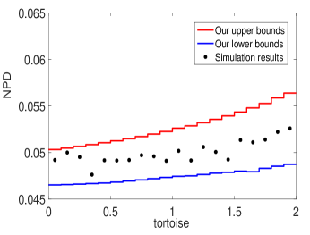
(b) Hare Tortoise Race v2

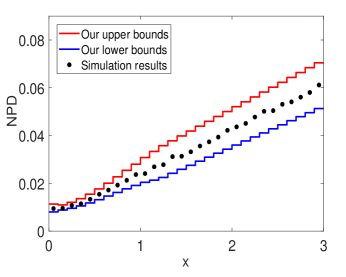
(c) Random Walk v1

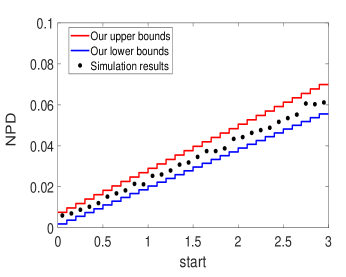
(d) Pedestrian Multi-branches v3

Figure 11. Part 1: NPD Bounds of Novel Examples

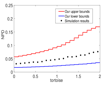
(a) Hare Tortoise Race v1

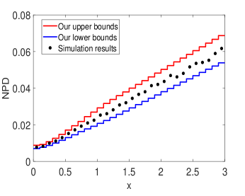
(b) Random Walk v2

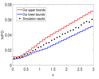
(c) Random Walk v3

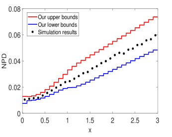
(d) Random Walk v4

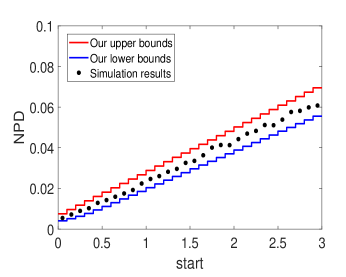
(e) Pedestrian Multi-branches v4

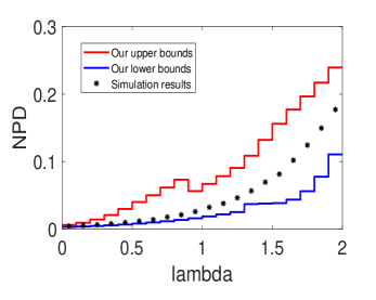
(f) Phylogenetic Birth Model

Figure 12. Part 2: NPD Bounds of Novel Examples

(a) Pedestrian

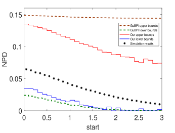
(b) Pedestrain Large Deviation

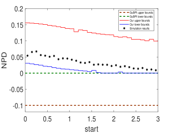
(c) Pedestrian Beta v1

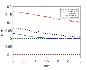
(d) Pedestrian Beta v2

Figure 13. Part 1: NPD Bounds of Our Approach and GuBPI

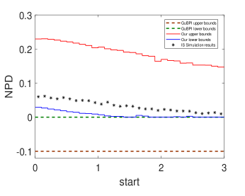
(a) Pedestrian Beta v3

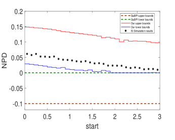
(b) Pedestrian Beta v4

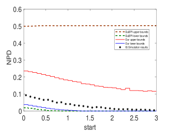
(c) Pedestrian Multi-branches v5

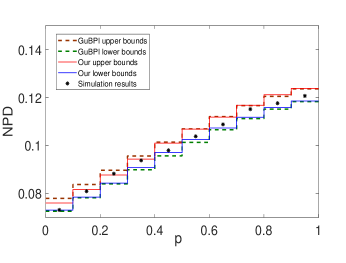
(d) Para Estimation Recursive

Figure 14. Part 2: NPD Bounds of Our Approach and GuBPI

References

- (1)
- ApS (2022) MOSEK ApS. 2022. The MOSEK optimization toolbox for MATLAB manual. Version 10.0. http://docs.mosek.com/10.0/toolbox/index.html
- Barthe et al. (2018) Gilles Barthe, Thomas Espitau, Benjamin Grégoire, Justin Hsu, and Pierre-Yves Strub. 2018. Proving expected sensitivity of probabilistic programs. Proc. ACM Program. Lang. 2, POPL (2018), 57:1–57:29. https://doi.org/10.1145/3158145
- Batz et al. (2023) Kevin Batz, Mingshuai Chen, Sebastian Junges, Benjamin Lucien Kaminski, Joost-Pieter Katoen, and Christoph Matheja. 2023. Probabilistic Program Verification via Inductive Synthesis of Inductive Invariants. In Tools and Algorithms for the Construction and Analysis of Systems - 29th International Conference, TACAS 2023, Held as Part of the European Joint Conferences on Theory and Practice of Software, ETAPS 2022, Paris, France, April 22-27, 2023, Proceedings, Part II (Lecture Notes in Computer Science, Vol. 13994), Sriram Sankaranarayanan and Natasha Sharygina (Eds.). Springer, 410–429. https://doi.org/10.1007/978-3-031-30820-8_25
- Beutner et al. (2022) Raven Beutner, C.-H. Luke Ong, and Fabian Zaiser. 2022. Guaranteed bounds for posterior inference in universal probabilistic programming. In PLDI ’22: 43rd ACM SIGPLAN International Conference on Programming Language Design and Implementation, San Diego, CA, USA, June 13 - 17, 2022, Ranjit Jhala and Isil Dillig (Eds.). ACM, 536–551. https://doi.org/10.1145/3519939.3523721
- Bingham et al. (2019) Eli Bingham, Jonathan P. Chen, Martin Jankowiak, Fritz Obermeyer, Neeraj Pradhan, Theofanis Karaletsos, Rohit Singh, Paul A. Szerlip, Paul Horsfall, and Noah D. Goodman. 2019. Pyro: Deep Universal Probabilistic Programming. J. Mach. Learn. Res. 20 (2019), 28:1–28:6. http://jmlr.org/papers/v20/18-403.html
- Blei et al. (2017) David M Blei, Alp Kucukelbir, and Jon D McAuliffe. 2017. Variational inference: A review for statisticians. Journal of the American statistical Association 112, 518 (2017), 859–877.
- Borgström et al. (2016) Johannes Borgström, Ugo Dal Lago, Andrew D. Gordon, and Marcin Szymczak. 2016. A lambda-calculus foundation for universal probabilistic programming. In Proceedings of the 21st ACM SIGPLAN International Conference on Functional Programming, ICFP 2016, Nara, Japan, September 18-22, 2016, Jacques Garrigue, Gabriele Keller, and Eijiro Sumii (Eds.). ACM, 33–46. https://doi.org/10.1145/2951913.2951942
- Chakarov and Sankaranarayanan (2013a) Aleksandar Chakarov and Sriram Sankaranarayanan. 2013a. Probabilistic Program Analysis with Martingales. In CAV 2013. 511–526.
- Chakarov and Sankaranarayanan (2013b) Aleksandar Chakarov and Sriram Sankaranarayanan. 2013b. Probabilistic Program Analysis with Martingales. In Computer Aided Verification - 25th International Conference, CAV 2013, Saint Petersburg, Russia, July 13-19, 2013. Proceedings (Lecture Notes in Computer Science, Vol. 8044), Natasha Sharygina and Helmut Veith (Eds.). Springer, 511–526. https://doi.org/10.1007/978-3-642-39799-8_34
- Chatterjee et al. (2016a) Krishnendu Chatterjee, Hongfei Fu, and Amir Kafshdar Goharshady. 2016a. Termination Analysis of Probabilistic Programs Through Positivstellensatz’s. In CAV 2016. 3–22.
- Chatterjee et al. (2020) Krishnendu Chatterjee, Hongfei Fu, Amir Kafshdar Goharshady, and Ehsan Kafshdar Goharshady. 2020. Polynomial invariant generation for non-deterministic recursive programs. In Proceedings of the 41st ACM SIGPLAN International Conference on Programming Language Design and Implementation, PLDI 2020, London, UK, June 15-20, 2020, Alastair F. Donaldson and Emina Torlak (Eds.). ACM, 672–687. https://doi.org/10.1145/3385412.3385969
- Chatterjee et al. (2016b) Krishnendu Chatterjee, Hongfei Fu, Petr Novotný, and Rouzbeh Hasheminezhad. 2016b. Algorithmic analysis of qualitative and quantitative termination problems for affine probabilistic programs. In Proceedings of the 43rd Annual ACM SIGPLAN-SIGACT Symposium on Principles of Programming Languages, POPL 2016, St. Petersburg, FL, USA, January 20 - 22, 2016, Rastislav Bodík and Rupak Majumdar (Eds.). ACM, 327–342. https://doi.org/10.1145/2837614.2837639
- Chatterjee et al. (2018) Krishnendu Chatterjee, Hongfei Fu, Petr Novotný, and Rouzbeh Hasheminezhad. 2018. Algorithmic Analysis of Qualitative and Quantitative Termination Problems for Affine Probabilistic Programs. ACM Trans. Program. Lang. Syst. 40, 2 (2018), 7:1–7:45. https://doi.org/10.1145/3174800
- Chatterjee et al. (2017) Krishnendu Chatterjee, Petr Novotný, and Đorđe Žikelić. 2017. Stochastic invariants for probabilistic termination. In POPL 2017. 145–160.
- Colón et al. (2003) Michael Colón, Sriram Sankaranarayanan, and Henny Sipma. 2003. Linear Invariant Generation Using Non-linear Constraint Solving. In Computer Aided Verification, 15th International Conference, CAV 2003, Boulder, CO, USA, July 8-12, 2003, Proceedings (Lecture Notes in Computer Science, Vol. 2725), Warren A. Hunt Jr. and Fabio Somenzi (Eds.). Springer, 420–432. https://doi.org/10.1007/978-3-540-45069-6_39
- De Moura and Bjørner (2008) Leonardo De Moura and Nikolaj Bjørner. 2008. Z3: An Efficient SMT Solver. In Proceedings of the Theory and Practice of Software, 14th International Conference on Tools and Algorithms for the Construction and Analysis of Systems (Budapest, Hungary) (TACAS’08/ETAPS’08). Springer-Verlag, Berlin, Heidelberg, 337–340.
- Fu and Chatterjee (2019) Hongfei Fu and Krishnendu Chatterjee. 2019. Termination of Nondeterministic Probabilistic Programs. In Verification, Model Checking, and Abstract Interpretation - 20th International Conference, VMCAI 2019, Cascais, Portugal, January 13-15, 2019, Proceedings (Lecture Notes in Computer Science, Vol. 11388), Constantin Enea and Ruzica Piskac (Eds.). Springer, 468–490. https://doi.org/10.1007/978-3-030-11245-5_22
- Gamerman and Lopes (2006) Dani Gamerman and Hedibert F Lopes. 2006. Markov chain Monte Carlo: stochastic simulation for Bayesian inference. CRC press.
- Gehr et al. (2016) Timon Gehr, Sasa Misailovic, and Martin T. Vechev. 2016. PSI: Exact Symbolic Inference for Probabilistic Programs. In Computer Aided Verification - 28th International Conference, CAV 2016, Toronto, ON, Canada, July 17-23, 2016, Proceedings, Part I (Lecture Notes in Computer Science, Vol. 9779), Swarat Chaudhuri and Azadeh Farzan (Eds.). Springer, 62–83. https://doi.org/10.1007/978-3-319-41528-4_4
- Gehr et al. (2020) Timon Gehr, Samuel Steffen, and Martin T. Vechev. 2020. PSI: exact inference for higher-order probabilistic programs. In Proceedings of the 41st ACM SIGPLAN International Conference on Programming Language Design and Implementation, PLDI 2020, London, UK, June 15-20, 2020, Alastair F. Donaldson and Emina Torlak (Eds.). ACM, 883–897. https://doi.org/10.1145/3385412.3386006
- Goodman et al. (2008) Noah D. Goodman, Vikash K. Mansinghka, Daniel M. Roy, Kallista A. Bonawitz, and Joshua B. Tenenbaum. 2008. Church: a language for generative models. In UAI 2008, Proceedings of the 24th Conference in Uncertainty in Artificial Intelligence, Helsinki, Finland, July 9-12, 2008, David A. McAllester and Petri Myllymäki (Eds.). AUAI Press, 220–229.
- Goodman and Stuhlmüller (2014) Noah D Goodman and Andreas Stuhlmüller. 2014. The Design and Implementation of Probabilistic Programming Languages. http://dippl.org.
- Gordon et al. (2014) Andrew D Gordon, Thomas A Henzinger, Aditya V Nori, and Sriram K Rajamani. 2014. Probabilistic programming. In Future of Software Engineering Proceedings. 167–181.
- Handelman (1988) David Handelman. 1988. Representing polynomials by positive linear functions on compact convex polyhedra. Pacific J. Math. 132, 1 (1988), 35–62.
- Huang et al. (2021) Zixin Huang, Saikat Dutta, and Sasa Misailovic. 2021. AQUA: Automated Quantized Inference for Probabilistic Programs. In Automated Technology for Verification and Analysis - 19th International Symposium, ATVA 2021, Gold Coast, QLD, Australia, October 18-22, 2021, Proceedings (Lecture Notes in Computer Science, Vol. 12971), Zhe Hou and Vijay Ganesh (Eds.). Springer, 229–246. https://doi.org/10.1007/978-3-030-88885-5_16
- Jeffreys (1988) H Jeffreys. 1988. "Weierstrass’s theorem on approximation by polynomials" and "Extension of Weierstrass’s approximation theory". Methods of Mathematical Physics (1988), 446–448.
- Kura et al. (2019) Satoshi Kura, Natsuki Urabe, and Ichiro Hasuo. 2019. Tail probabilities for randomized program runtimes via martingales for higher moments. In International Conference on Tools and Algorithms for the Construction and Analysis of Systems. Springer, 135–153.
- Lee et al. (2020) Wonyeol Lee, Hangyeol Yu, Xavier Rival, and Hongseok Yang. 2020. Towards verified stochastic variational inference for probabilistic programs. Proc. ACM Program. Lang. 4, POPL (2020), 16:1–16:33. https://doi.org/10.1145/3371084
- Mak et al. (2021) Carol Mak, C.-H. Luke Ong, Hugo Paquet, and Dominik Wagner. 2021. Densities of Almost Surely Terminating Probabilistic Programs are Differentiable Almost Everywhere. In Programming Languages and Systems - 30th European Symposium on Programming, ESOP 2021, Held as Part of the European Joint Conferences on Theory and Practice of Software, ETAPS 2021, Luxembourg City, Luxembourg, March 27 - April 1, 2021, Proceedings (Lecture Notes in Computer Science, Vol. 12648), Nobuko Yoshida (Ed.). Springer, 432–461. https://doi.org/10.1007/978-3-030-72019-3_16
- McIver and Morgan (2004) Annabelle McIver and Carroll Morgan. 2004. Developing and Reasoning About Probabilistic Programs in pGCL. In Refinement Techniques in Software Engineering, First Pernambuco Summer School on Software Engineering, PSSE 2004, Recife, Brazil, November 23-December 5, 2004, Revised Lectures (Lecture Notes in Computer Science, Vol. 3167), Ana Cavalcanti, Augusto Sampaio, and Jim Woodcock (Eds.). Springer, 123–155. https://doi.org/10.1007/11889229_4
- McIver and Morgan (2005) Annabelle McIver and Carroll Morgan. 2005. Abstraction, Refinement and Proof for Probabilistic Systems. Springer. https://doi.org/10.1007/b138392
- Meyn and Tweedie (2012) Sean P Meyn and Richard L Tweedie. 2012. Markov chains and stochastic stability. Springer Science & Business Media.
- Narayanan et al. (2016) Praveen Narayanan, Jacques Carette, Wren Romano, Chung-chieh Shan, and Robert Zinkov. 2016. Probabilistic Inference by Program Transformation in Hakaru (System Description). In Functional and Logic Programming - 13th International Symposium, FLOPS 2016, Kochi, Japan, March 4-6, 2016, Proceedings (Lecture Notes in Computer Science, Vol. 9613), Oleg Kiselyov and Andy King (Eds.). Springer, 62–79. https://doi.org/10.1007/978-3-319-29604-3_5
- Ngo et al. (2018) Van Chan Ngo, Quentin Carbonneaux, and Jan Hoffmann. 2018. Bounded expectations: resource analysis for probabilistic programs. In Proceedings of the 39th ACM SIGPLAN Conference on Programming Language Design and Implementation, PLDI 2018, Philadelphia, PA, USA, June 18-22, 2018, Jeffrey S. Foster and Dan Grossman (Eds.). ACM, 496–512. https://doi.org/10.1145/3192366.3192394
- Pollard (2002) David Pollard. 2002. A user’s guide to measure theoretic probability. Number 8. Cambridge University Press.
- Putinar (1993) Mihai Putinar. 1993. Positive Polynomials on Compact Semi-algebraic Sets. Indiana University Mathematics Journal 42, 3 (1993), 969–984. http://www.jstor.org/stable/24897130
- Rankin (1968) RA Rankin. 1968. Real and Complex Analysis. By W. Rudin. Pp. 412. 84s. 1966.(McGraw-Hill, New York.). The Mathematical Gazette 52, 382 (1968), 412–412.
- Ronquist et al. (2021) Fredrik Ronquist, Jan Kudlicka, Viktor Senderov, Johannes Borgström, Nicolas Lartillot, Daniel Lundén, Lawrence Murray, Thomas B Schön, and David Broman. 2021. Universal probabilistic programming offers a powerful approach to statistical phylogenetics. Communications biology 4, 1 (2021), 1–10.
- Rubinstein and Kroese (2016) Reuven Y Rubinstein and Dirk P Kroese. 2016. Simulation and the Monte Carlo method. Vol. 10. John Wiley & Sons.
- Rudin et al. (1976) Walter Rudin et al. 1976. Principles of mathematical analysis. Vol. 3. McGraw-hill New York.
- Saad et al. (2021) Feras A. Saad, Martin C. Rinard, and Vikash K. Mansinghka. 2021. SPPL: probabilistic programming with fast exact symbolic inference. In PLDI ’21: 42nd ACM SIGPLAN International Conference on Programming Language Design and Implementation, Virtual Event, Canada, June 20-25, 2021, Stephen N. Freund and Eran Yahav (Eds.). ACM, 804–819. https://doi.org/10.1145/3453483.3454078
- Sangiorgi (2011) Davide Sangiorgi. 2011. Introduction to bisimulation and coinduction. Cambridge University Press.
- Sankaranarayanan et al. (2013) Sriram Sankaranarayanan, Aleksandar Chakarov, and Sumit Gulwani. 2013. Static analysis for probabilistic programs: inferring whole program properties from finitely many paths. In ACM SIGPLAN Conference on Programming Language Design and Implementation, PLDI ’13, Seattle, WA, USA, June 16-19, 2013, Hans-Juergen Boehm and Cormac Flanagan (Eds.). ACM, 447–458. https://doi.org/10.1145/2491956.2462179
- Sankaranarayanan et al. (2004) Sriram Sankaranarayanan, Henny B. Sipma, and Zohar Manna. 2004. Constraint-Based Linear-Relations Analysis. In Static Analysis, 11th International Symposium, SAS 2004, Verona, Italy, August 26-28, 2004, Proceedings (Lecture Notes in Computer Science, Vol. 3148), Roberto Giacobazzi (Ed.). Springer, 53–68. https://doi.org/10.1007/978-3-540-27864-1_7
- Staton et al. (2016) Sam Staton, Hongseok Yang, Frank D. Wood, Chris Heunen, and Ohad Kammar. 2016. Semantics for probabilistic programming: higher-order functions, continuous distributions, and soft constraints. In Proceedings of the 31st Annual ACM/IEEE Symposium on Logic in Computer Science, LICS ’16, New York, NY, USA, July 5-8, 2016, Martin Grohe, Eric Koskinen, and Natarajan Shankar (Eds.). ACM, 525–534. https://doi.org/10.1145/2933575.2935313
- Tarski (1955) Alfred Tarski. 1955. A lattice-theoretical fixpoint theorem and its applications. Pacific journal of Mathematics 5, 2 (1955), 285–309.
- Tolpin et al. (2015) David Tolpin, Jan-Willem van de Meent, and Frank D. Wood. 2015. Probabilistic Programming in Anglican. In Machine Learning and Knowledge Discovery in Databases - European Conference, ECML PKDD 2015, Porto, Portugal, September 7-11, 2015, Proceedings, Part III (Lecture Notes in Computer Science, Vol. 9286), Albert Bifet, Michael May, Bianca Zadrozny, Ricard Gavaldà, Dino Pedreschi, Francesco Bonchi, Jaime S. Cardoso, and Myra Spiliopoulou (Eds.). Springer, 308–311. https://doi.org/10.1007/978-3-319-23461-8_36
- van de Meent et al. (2018) Jan-Willem van de Meent, Brooks Paige, Hongseok Yang, and Frank Wood. 2018. An Introduction to Probabilistic Programming. CoRR abs/1809.10756 (2018). arXiv:1809.10756
- Wang et al. (2021a) Di Wang, Jan Hoffmann, and Thomas W. Reps. 2021a. Central moment analysis for cost accumulators in probabilistic programs. In PLDI ’21: 42nd ACM SIGPLAN International Conference on Programming Language Design and Implementation, Virtual Event, Canada, June 20-25, 2021, Stephen N. Freund and Eran Yahav (Eds.). ACM, 559–573. https://doi.org/10.1145/3453483.3454062
- Wang et al. (2021b) Jinyi Wang, Yican Sun, Hongfei Fu, Krishnendu Chatterjee, and Amir Kafshdar Goharshady. 2021b. Quantitative analysis of assertion violations in probabilistic programs. In PLDI ’21: 42nd ACM SIGPLAN International Conference on Programming Language Design and Implementation, Virtual Event, Canada, June 20-25, 2021, Stephen N. Freund and Eran Yahav (Eds.). ACM, 1171–1186. https://doi.org/10.1145/3453483.3454102
- Wang (2022) Peixin Wang. 2022. Tail-Bound Cost Analysis over Nondeterministic Probabilistic Programs. Journal of Shanghai Jiaotong University (Science) (2022), 1–11.
- Wang et al. (2020) Peixin Wang, Hongfei Fu, Krishnendu Chatterjee, Yuxin Deng, and Ming Xu. 2020. Proving expected sensitivity of probabilistic programs with randomized variable-dependent termination time. Proc. ACM Program. Lang. 4, POPL (2020), 25:1–25:30. https://doi.org/10.1145/3371093
- Wang et al. (2019) Peixin Wang, Hongfei Fu, Amir Kafshdar Goharshady, Krishnendu Chatterjee, Xudong Qin, and Wenjun Shi. 2019. Cost Analysis of Nondeterministic Probabilistic Programs. In Proceedings of the 40th ACM SIGPLAN Conference on Programming Language Design and Implementation (Phoenix, AZ, USA) (PLDI 2019). Association for Computing Machinery, New York, NY, USA, 204–220. https://doi.org/10.1145/3314221.3314581
- Williams (1991) David Williams. 1991. Probability with martingales. Cambridge university press.