The Fagnano Triangle Patrolling Problem

Abstract

We investigate a combinatorial optimization problem that involves patrolling the edges of an acute triangle using a unit-speed agent. The goal is to minimize the maximum (1-gap) idle time of any edge, which is defined as the time gap between consecutive visits to that edge. This problem has roots in a centuries-old optimization problem posed by Fagnano in 1775, who sought to determine the inscribed triangle of an acute triangle with the minimum perimeter. It is well-known that the orthic triangle, giving rise to a periodic and cyclic trajectory obeying the laws of geometric optics, is the optimal solution to Fagnano's problem. Such trajectories are known as Fagnano orbits, or more generally as billiard trajectories. We demonstrate that the orthic triangle is also an optimal solution to the patrolling problem.

Our main contributions pertain to new connections between billiard trajectories and optimal patrolling schedules in combinatorial optimization. In particular, as an artifact of our arguments, we introduce a novel 2-gap patrolling problem that seeks to minimize the visitation time of objects every three visits. We prove that there exist infinitely many well-structured billiard-type optimal trajectories for this problem, including the orthic trajectory, which has the special property of minimizing the visitation time gap between any two consecutively visited edges. Complementary to that, we also examine the cost of dynamic, sub-optimal trajectories to the 1-gap patrolling optimization problem. These trajectories result from a greedy algorithm and can be implemented by a computationally primitive mobile agent.

1 Introduction

Patrolling refers to the perpetual monitoring, protection, and supervision of a domain or its perimeter using mobile agents. In a typical patrolling problem involving one mobile agent, the agent must move through a given domain in order to monitor or check specific locations or objects. The objective is to find a trajectory that satisfies certain constraints and/or that addresses quantitative objectives, such as minimizing the total distance traveled or maximizing the frequency of visits to certain areas. The purpose of patrolling could be to detect any intrusion attempts, monitor for possible faults or to identify and rescue individuals or objects in a disaster environment, and for this reason, such problems arise in a variety of real-world applications, such as security patrol routes, autonomous robot navigation, and wildlife monitoring. Overall the subject of patrolling has seen a growing number of applications in Computer Science, including Infrastructure Security, Computer Games, perpetual domain-surveying, and monitoring in 1D and 2D geometric domains.

In addition to its practical applications, patrolling has emerged (not as a combinatorial optimization problem) in the context of theoretical physics. In particular, the problem of finding periodic trajectories in billiard systems has been a topic of interest for many years. A billiard system is a model of a particle or a waveform moving inside a domain (typically polygonal, but also elliptical, convex, or even non-convex region) and reflecting off its boundaries according to the laws of elastic collision. The problem of finding periodic trajectories in a billiard system is equivalent to finding a closed path in the domain that satisfies certain geometric conditions.

One important example of a periodic trajectory in billiard systems is the so-called Fagnano orbit on acute triangles, a periodic, closed (and piece-wise linear) curve that visits the three edges of an acute triangle. Fagnano orbits, named after the Italian mathematician Giulio Fagnano who first studied them in the mid-18th century, arise as solutions to the optimization problem which asks for the shortest such curve. In this work we explore further connections between billiard trajectories and patrolling as a combinatorial optimization problem. In particular, we are asking what are the patrolling strategies for the edges of an acute triangle that optimize standard frequency-related objectives are. Our findings demonstrate that a family of Fagnano orbits are actually optimal solutions to the corresponding combinatorial optimization problems, revealing this way deeper connections between the seemingly disparate areas of combinatorial patrolling and billiard trajectories.

2 Related Work

Patrolling problems are a fundamental class of problems in computational geometry, combinatorial optimization, and robotics that have attracted significant research interest in recent years. Due to their practical applications, they have received extensive treatment in the realm of robotics, see for example [1, 6, 14, 15, 21, 30, 40], as well as surveys [3, 22, 34]. When patrolling is seen as part of infrastructure security, it leads to a number of optimization problems [26], with one particular example being the identification of network failures or web pages requiring indexing [30].

Combinatorial trade-offs of triangle edge visitation costs have been explored in [19]. In contrast, the current work pertains to the cost associated with the perpetual monitoring of the triangle edges by a single unit speed agent. Numerous variations of similar patrolling problems have been explored in computational geometry, which vary depending on the application domain, patrolling specifications, agent restrictions, and computational abilities. Many efficient algorithms have been developed for several of these variants, utilizing a range of techniques from graph theory, computational geometry, and optimization, see survey [10] for some recent developments. Some examples of studied domains include the bounded line segment [24], networks [41], polygonal regions [37], trees [11], disconnected boundaries of one dimensional curves [8], arbitrary polygonal environments [32] (with a reduction to graphs), or even 3-dimensional environments [16].

Identifying optimal patrolling strategies can be computationally hard [12], while even in seemingly easy setups the optimal trajectories can be counter-intuitive [25]. The addition of combinatorial specifications has given rise to multiple intriguing variations, including the requirement of uneven coverage [7, 33] or waiting times [13], the presence of high-priority segments [31], and patrolling with distinct speed agents [9]. Patrolling has also been studied extensively from the perspective of distributed computing [29], while the class of these problems also admit a game-theoretic interpretation between an intruder and a surveillance agent [2, 18].

Maybe not surprisingly, the optimal patrolling trajectories that we derive are in fact billiard-type trajectories, that is, periodic and cyclic trajectories obeying the standard law of geometric optics, and which are referred to as Fagnano orbits specifically when the underlying billiard/domain is triangular. Fagnano orbits have been studied extensively both experimentally [27] and theoretically [38]. Billiard-type trajectories have been explored in equilateral triangles [4], obtuse triangles [20], as well as polygons [39]. More recently, there have been studies on ellipses [17] and general convex bodies [23], or even fractals [28] and polyhedra [5], with the list of domains or trajectory specifications still growing.

3 Main Definitions and Results

A patrolling schedule $S$ (or simply a schedule) for triangle $\Delta$ with edges (line segments) $E=\{\alpha,\beta,\gamma\}$ is an infinite sequence $\{s_{i}\}_{i\geq 0}$, where each $s_{i}$ is on a line segment of $E$ that we also denote by $e(s_{i})$, i.e. $e(s_{i})\in E$ for each $i\geq 0$. When $e(s_{i})=\delta\in E$ we say that segment $\delta$ and point $s_{i}$ are visited at step $i$ of the schedule. We will only be studying feasible schedules, i.e. schedules for which eventually all segments in $E$ are visited (and infinitely often).

For simplicity, our notation above is tailored to points $s_{i}$ that are not vertices of $\Delta$. When $s_{i}$ is a vertex of $\Delta$ we assume that both incident edges are visited. We also think of schedule $S$ as the trajectory of a unit speed agent, and hence we refer to the time between the visitation of $s_{j},s_{j+\ell}$ as the summation of the lengths of segments $s_{j+i}s_{j+i+1}$ over $i\in\{0,\ldots,\ell-1\}$.

A schedule $S$ is called:
- cyclic if $\{e(s_{0}),e(s_{1}),e(s_{2})\}=E$ and $e(s_{i+3})=e(s_{i})$, for every $i\geq 0$, and
- $k$-periodic (for $k\geq 3$) if $s_{i+k}=s_{i}$, for every $i\geq 0$.

For any segment $\delta\in E$ we define its $t$-gap sequence, $g^{t}(\delta)$, that records the visitation time gaps of $\delta$ over every $t+1$ consecutive visitations. In particular, $t=1$ corresponds to the standard idle time considered previously, and that measures the additional time it takes for each object to be revisited, after each visitation. Formally, let $e(s_{j})=e(s_{j^{\prime}})=\delta$ and suppose that points $s_{j},s_{j^{\prime}}$ are the $k$-th and $(k+t)$-th visitation of $\delta$, respectively. Then the time between the visitations of $s_{j},s_{j^{\prime}}$ is exactly the value of $k$-th element of sequence $g^{t}(\delta)$. From this definition, it is also immediate that $\left(g^{t}(\delta)\right)_{i}=\sum_{i=1}^{t}\left(g^{1}(\delta)\right)_{i}$.

The $t$-gap $G^{t}(\delta)$ of $\delta\in E$ is defined as $\sup_{i}\left(g^{t}(\delta)\right)_{i}$, while the $t$-gap $G^{t}$ of schedule $S$ for edges $E$ (hence for input triangle $\Delta$) is defined as $\max_{\delta\in E}G^{t}(\delta)$. When it is clear from the context, we will abbreviate $G^{1}$ simply by $G$.

3.1 Main Contributions & More Terminology

In this section we summarize our main contributions, pertaining to the optimal $1$-gap and $2$-gap patrolling schedules of acute triangles.

As a warm-up, we first give a self-contained proof of optimality for $1$-gap patrolling schedules, restricted to cyclic and $3$-periodic schedules. In order to present our result, we remind the reader of the so-called orthic triangle, a pedal-type triangle of an acute triangle $\Delta$, which is a triangle inscribed in $\Delta$ whose vertices are the projections of the $\Delta$'s orthocenter (intersection of altitudes) to its three edges. Note also the any $3$-periodic cyclic schedule corresponds to a triangle inscribed in $\Delta$. The next theorem, given first by Fagnano in 1775, is proven in Section 4, where we also introduce some key concepts for our follow-up main contributions.

Theorem 3.1 (Fagnano's Theorem)

The optimal $1$-gap $3$-periodic cyclic patrolling schedule of a triangle $\Delta$ is its orthic triangle.

Towards our goal to provide the optimal $1$-gap schedules, we find all (infinitely many) optimal $2$-gap cyclic schedules, which are in fact billiard-type trajectories. We prove the next theorem in Section 6.

Theorem 3.2

There are infinitely many optimal $2$-gap cyclic schedules of a triangle $\Delta$, that include also the orthic triangle. Every $2$-gap optimal schedule is $6$-periodic and has value equal to 2 times the perimeter of the orthic triangle. Moreover, each optimal schedule is made up of segments that are parallel to the edges of the orthic triangle.

Then in Section 7 we derive our main contribution.

Theorem 3.3

The optimal $1$-gap schedule of a triangle $\Delta$ is its orthic triangle.

In the same section we also quantify the $1$-gap cost of the orthic triangle, and we compare it to the optimal $2$-gap schedules. Indeed, we ask which of the optimal $2$-gap schedules minimizes the maximum time in-between the visitation of any two edges of $\Delta$ (and not of the same edge), and we prove that the orthic schedule is again the optimal, in this multi-objective optimization problem.

From our previous contributions, we conclude that a mobile agent whose task is to $1$-gap optimally patrol a triangle $\Delta$ needs to be able to compute the base points of $\Delta$'s altitudes. Therefore, a natural question is whether we can obtain efficient solutions with a primitive agent. In Section 8 we show the following result.

Theorem 3.4

There is a greedy-type schedule that converges to a  $3$-periodic cyclic schedule whose $1$-gap cost is off from the $1$-gap optimal cyclic schedule by a factor $\gamma\in[1,\gamma_{0}]$, where $\gamma_{0}=\sqrt{2}/2+1/2$, and $\gamma$ admits a closed formula as a function of the angles of the given triangle.

It will follow from our analysis that our greedy algorithm will be nearly optimal for any acute triangle with one arbitrarily small angle, and it will be the worst off from the optimal solution when the given triangle is a right isosceles.

4 The $1$-Gap Optimal $3$-Periodic Cyclic Schedule

There are many proofs known for the fact that inscribed triangle with the shortest perimeter is its orthic triangle. In the language of triangle patrolling, the statement is equivalent to that that the optimal $1$-gap $3$-periodic cyclic schedule of a triangle is its orthic triangle, articulated in Theorem 3.1. For completeness, we provide next a self-contained proof.

Proof (Proof of Theorem 3.1)

We consider triangle $ABC$, as in Figure 1. First we find the inscribed triangle of minimum perimeter, and then we show the optimizer is the orthic triangle.

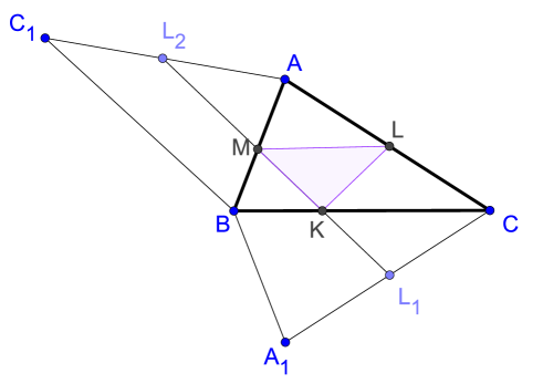
Figure 1: Triangle figure supporting the proof of Fagnano's Theorem.

We start with an arbitrary point $L$ on $AC$, and we find the optimal points $K,M$ on $BC,AB$, respectively, so as to minimize the perimeter of $KLM$ as a function of $L$. Then, we show how to choose $L$ so as to minimize the perimeter.

Consider the reflection $A_{1}$ of $A$ about $BC$, the reflection $C_{1}$ of $C$ about $AB$, and the reflections $L_{1},L_{2}$ of $L$ about $BC,AB$, respectively. Consider also the intersections $K,M$ of $L_{1}{\color[rgb]{1,0,0}\textbf{\textst{,}}}L_{2}$ with $BC,AB$, respectively. Clearly, the optimal way to start from $L$, visit edge $BC$, then $AB$ and then return to $L$ is by following the edges of triangle $KLM$. Moreover, the perimeter of $KLM$ equals segment $L_{1}L_{2}$. Next we minimize the length of $L_{1}L_{2}$ as a function of $L$.

In this direction, we consider a Cartesian system centered at $B$ where $A=(p,q),B=(0,0),C=(1,0)$ (in particular, w.l.o.g. we assume that $BC=1$). Note that $A_{1}=(p,-q),C_{1}=(\cos(2B),\sin(2B))$, where also

$$p=\frac{\cos(B)\sin(C)}{\sin(B+C)},~{}~{}q=\frac{\sin(B)\sin(C)}{\sin(B+C)}.$$ (1)

Point $L$ is a convex combination of $A,C$, hence there exists $x\in[0,1]$ such that $L=xC+(1-x)A$. Therefore, $L_{1}=xC+(1-x)A_{1},~{}~{}L_{2}=xC_{1}+(1-x)A,$ so that

$$\left\lVert L_{1}-L_{2}\right\rVert^{2} =\left\lVert x(C-C_{1})+(1-x)(A_{1}-A)\right\rVert^{2}$$

$$=\left\lVert x\left(\begin{array}[]{c}\cos(2B)-1\\ \sin(2B)\end{array}\right)+(1-x)\left(\begin{array}[]{l}0\\ 2q\end{array}\right)\right\rVert^{2}.$$

It follows that $\left\lVert L_{1}-L_{2}\right\rVert^{2}$ is convex in $x$ (degree 2 polynomial), and elementary calculations show that the minimum is attained at $x_{0}=\frac{\cos(A)\sin(C)}{\sin(B)}.$ It can be seen that for all acute triangles, we have $x_{0}\in[0,1]$. Then, the minimum patrolling trajectory has length

$$\left\lVert x_{0}(C-C_{1})+(1-x_{0})(A_{1}-A)\right\rVert=2\sin(B)\sin(C).$$

Note that the choice of $x_{0}$ determines all points $K,L,M$. Now we show that $KLM$ is the orthic triangle. In order to show that $K$ is the base of the altitude corresponding to $A$, we verify that points $(p,0),L_{1},L_{2}$ are collinear (and hence $K=(p,0)$). For this observe that $L_{1},L_{2}$ are already expressed as a function of $p,q,x_{0}$, and hence the claim follows by straightforward calculations.

Next we show that $L$ is the base of the altitude corresponding to $B$. For this we verify that $KL$ is perpendicular to $AC$. Indeed, $L=x_{0}C+(1-x_{0})A,~{}~{}L_{2}=x_{0}C_{1}+(1-x_{0})A=(x_{0}+(1-x_{0})p,(1-x_{0})q),$ while vector $AC$ is $(1-p,-q)$. Taking the inner product of the vectors gives $(x_{0}+(1-x_{0})p)(1-p)-(1-x_{0})q^{2}$ which, after elementary calculations reduces to $0$, as promised.

Finally, we verify that $M$ is the base of the altitude corresponding to $C$. For this, we compute the projection of $C=(1,0)$ onto the line passing through $A,B$ which reads as $py-qx=0$, which is point $\frac{p}{p^{2}+q^{2}}(p,q)$. Finally, elementary calculations can verify that the latter point, together with $K,L_{2}$ are collinear, and hence $M=\frac{p}{p^{2}+q^{2}}(p,q)$ as promised. ∎

The next complementary lemma effectively provides a formula for the optimal $1$-gap cost of cyclic 3-periodic schedules.

Lemma 1

Let $p$ be the perimeter of an acute triangle. Then, the perimeter of its orthic triangle is given by

$$2p\left(\frac{1}{\sin(B)\sin(C)}+\frac{1}{\sin(A)\sin(C)}+\frac{1}{\sin(A)\sin(B)}\right)^{-1}.$$ (2)

Proof

As in the proof of Theorem 3.1 we assume that $A=(p,q),B=(0,0),C=(1,0)$ and hence that $\alpha=1$. From the derived formulas for the coordinates of points $K,L,M$ we have that

$$\left\lVert K-L\right\rVert =\frac{1}{2}\csc(B+C)\sin(2C)$$

$$\left\lVert K-M\right\rVert =\frac{1}{2}\csc(B+C)\sin(2B)$$

$$\left\lVert K-L\right\rVert =\cos(B+C).$$

But then, elementary trigonometric calculations give

$$\left\lVert K-L\right\rVert+\left\lVert K-M\right\rVert+\left\lVert K-L\right\rVert=2\sin(B)\sin(C).$$

It follows that for arbitrary edge length $\alpha$ (not necessarily equal to 1), we have that the perimeter of the orthic triangle equals $X=2\alpha\sin(B)\sin(C)$. Due to the symmetry of the formula, the perimeter must be also equal to $2\beta\sin(A)\sin(C)$ and to $2\gamma\sin(A)\sin(B)$. We conclude that

$$\alpha=\frac{X}{2\sin(B)\sin(C)},~{}~{}\beta=\frac{X}{2\sin(A)\sin(C)},~{}~{}\gamma=\frac{X}{2\sin(A)\sin(B)}.$$

So if we denote by $p$ the perimeter of the given triangle, i.e. $p=\alpha+\beta+\gamma$, adding the previous equations and solving for $X$ gives the promised formula. ∎

5 Technical Properties of the Orthic Patrolling Schedule

In this section we explore a number of technical properties associated with the orthic patrolling schedule, which will be the cornerstone of our main results. All observations in this section refer to Figure 2 which we explain gradually as we present our findings.

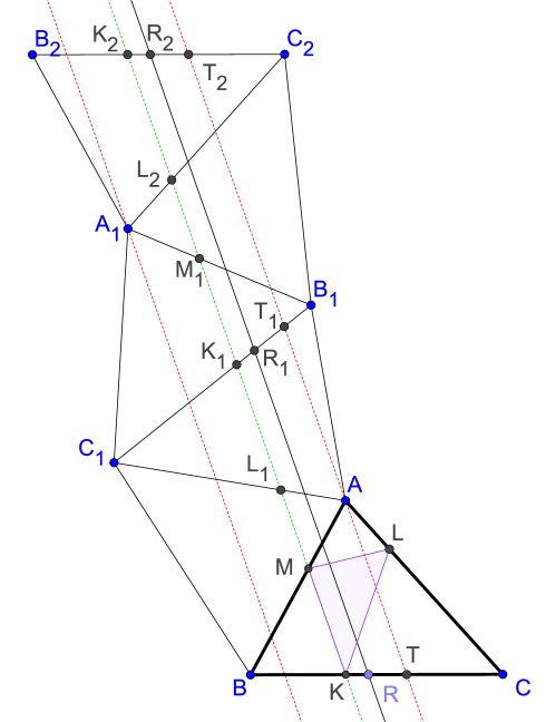
Figure 2: The orthic channel (stripe enclosed between the red dotted lines) as it is obtained by 5 triangle reflections.

Our starting point is triangle $ABC$ with edges $\alpha\geq\beta\geq\gamma$, and hence the same relation holds for the opposite angles. We also depict the base points $K,L,K$ of altitudes corresponding to $A,B,C$ respectively. It follows that inscribed triangle $KLM$ is the orthic triangle.

We apply a number of reflections of triangle $ABC$ as follows: we obtain reflection $C_{1}$ of $C$ around $AB$, reflection $B_{1}$ of $B$ around $AC_{1}$, reflection $A_{1}$ of $A$ around $B_{1}C_{1}$, reflection $C_{2}$ of $C_{1}$ around $A_{1}B_{1}$, and reflection $B_{2}$ of $B_{1}$ around $A_{1}C_{2}$. We refer to the resulting triangles as the reflected triangles.

Lemma 2

The line passing through $B_{2},C_{2}$ is parallel to line passing through $BC$.

Proof

We consider the slope of several line segments relevant to $BC$. We have the following observations pertaining to counterclockwise rotation of line segments about one of their endpoints. The rotation of $BC$ about $B$ by angle $2B$ gives segment $BC_{1}$. The rotation of $BC_{1}$ about $C_{1}$ by angle $3C$ gives segment $C_{1}A_{1}$. The rotation of $C_{1}A_{1}$ about $A_{1}$ by angle $3A$ gives segment $A_{1}B_{2}$. Finally, the rotation of $A_{1}B_{2}$ about $B_{2}$ by angle $B$ gives segment $B_{2}C_{2}$.

It follows that segment $B_{2}C_{2}$ follows by repeated rotation of angle $2B+3C+3A+B=3(A+B+C)=6\pi.$ Since $6\pi$ is a multiple of $\pi$ we conclude the claim. ∎

Next we provide an alternative representation of the orthic trajectory.

Lemma 3

The line passing through MK (green dotted line in Figure 2) passes through the following points: $L_{1}$ on $AC_{1}$, $K_{1}$ on $B_{1}C_{1}$, $M_{1}$ on $A_{1}B_{1}$, $L_{2}$ on $A_{1}C_{2}$, and $K_{2}$ on $B_{2}C_{2}$. Moreover, points $L_{1},K_{1},M_{1},L_{2},K_{2}$ are the bases of corresponding altitudes in the series of the reflected triangles.

Proof

By the proof of Theorem 3.1, the orthic triangle $KLM$ can be obtained by considering the image $K_{1}$ of $K$ (on $B_{1}C_{1}$) along the same reflections that resulted into the reflected triangles. Now consider the intersections $M,L_{1}$ of $KK_{1}$ with $AB,AC_{1}$, respectively. It follows that $CM$ and $C_{1}M$ are altitudes in triangles $ABC,ABC_{1}$, and $BL_{1}$ and $B_{1}L_{1}$ are altitudes in triangles $ABC_{1},AB_{1}C_{1}$. In particular, it follows that $K,M,L_{1},K_{1}$ are collinear.

The same argument applies if we start from triangle $AB_{1}C_{1}$ and invoke the same reflections starting from the third one, in the series that gave us the reflected triangles. It follows that by extending line $KK_{1}$ we intersect segment $A_{1}B_{1}$ at a point $M_{1}$, and segment $A_{1}C_{2}$ at a point $L_{2}$, where $C_{1}M_{1}$ and $C_{2}M_{1}$ are altitudes in triangles $A_{1}B_{1}C_{1}$, and $B_{1}L_{2}$ is altitudes in triangles $A_{1}B_{1}C_{2}$. Hence, $L_{2},M_{1},K_{1},L_{1},M,K$ are also collinear.

Finally, we observe that the base $K_{2}$ of altitude $A_{1}K_{2}$ is obtained as the reflection of $K_{1}$ using the last two reflections of the series of reflections that gave us the reflected triangles. It follows that $K_{2}$ is also collinear with $L_{2}$ and $M_{1}$ concluding our argument. ∎

It follows from Lemma 3 that the orthic trajectory along two cycles of the patrolling schedule can also be described by the line segment $K_{1}K_{2}$. We refer to the line passing through $K,K_{2}$ as the orthic line. Alternatively, we showed that all points within segment $K_{1}K_{2}$ lie within the reflected triangles. Our observation justifies that the following concept is well-defined.

Definition 1

The orthic channel is defined by two lines $\ell_{1},\ell_{2}$ parallel to the orthic line of maximum distance, and with the following properties: $\ell_{1},\ell_{2}$ intersect segments $BC$ and $B_{2}C_{2}$ and all points on lines $\ell_{1},\ell_{2}$ in-between segments $BC$ and $B_{2}C_{2}$ lie within the reflected triangles.

Similar reflection-induced channels were studied in [35, 36], while the orthic-channel that we use was also observed experimentally in [27]. Next we formalize its usefulness.

Lemma 4

Any line parallel to the orthic line within the orthic channel gives rise to a cyclic $6$-periodic patrolling schedule with $2$-gap cost equal to twice the orthic perimeter.

Proof

Consider an arbitrary line, parallel to the orthic line, that intersects line segments $BC,B_{1}C_{1},B_{2}C_{2}$ at points $R,R_{1},R_{2}$ respectively, see Figure 2. We observe that $KK2$ is parallel to $RR_{2}$, and by Lemma 2 we have that $K_{2}R_{2}$ is parallel to $KR$. Therefore, $KRR_{2}K_{2}$ is a parallelogram with $KR=KR_{2}$.

We conclude that $R_{2}$ is the reflection of $R$ using the same reflections that obtained $K_{2}$ from $K$. But then, it follows $RR_{2}$ corresponds to cyclic $6$-periodic patrolling schedule of $2$-gap cost equal to $RR_{2}=KK_{2}=KK_{1}+K_{1}K2=2KK1$, as promised. ∎

Next we identify all cyclic $6$-periodic patrolling schedules of the same $2$-gap costs. We note that in the following lemma we make explicit use of that the repeated reflections were done first along the smallest two edges.

Lemma 5

The lines identifying the orthic channel are the two lines parallel to the orthic line, one passing through $A$ and one passing through $A_{1}$.

Proof

Consider a line parallel to the orthic line passing through $A$, and intersecting $BC$ at $T$ and the line passing through $B_{1}C_{1}$ at point $T_{1}$. We will show that $T_{1}$ lies in the segment $K_{1}B_{1}$.

First we claim that $KT=K_{1}T_{1}$. To see why, recall that $KK_{1}$ is parallel to $TT_{1}$. It is enough to show that $KTT_{1}K_{1}$ is an isosceles trapezoid. Indeed, note that angle $AT_{1}C_{1}$ (read counterclockwise) equals angle $KK_{1}C$ (because $TT_{1}$ is parallel to $KK_{1}$), and angle $KK_{1}C$ equals angle $BKM$ (because $KK_{1}$ corresponds to the orthic trajectory that results from reflections). Finally, angle $BKM$ equals angle $BTT_{1}$, because $TT_{1}$ is parallel to $KK_{1}$. Overall, this shows that indeed, angles $KTT_{1}$ and $TT_{1}K_{1}$ are equal, showing that $KTT_{1}K_{1}$ is an isosceles trapezoid as claimed.

We conclude that in order to show that $T_{1}$ lies within segment $K_{1}B_{1}$ it is enough to show that $KT<KB$. Equivalently, it is enough to show that the middle point of $BT$ lies within segment $BK$. To see why recall that $AT$ is parallel to $MK$. Moreover, because angle $A$ is at least as large as angle $B$ (that is our initial reflections where done using the largest edge last), it follows that the base $M$ of altitude $CM$ is closer to $A$ than to $B$. Effectively, this shows that $BM\geq AB/2$, and hence $BK\geq BT/2$ as wanted.

Now let the extention of $TT_{1}$ intersect the line passing through $B_{2}C_{2}$ at point $T_{2}$. From the parallelogram $KTT_{2}K_{2}$ we have that $KT=K_{2}T_{2}$, and hence $T_{2}$ lies within segment $K_{2}C_{2}$, and by construction is it clear than $T_{1}T_{2}$ intersect segments $A_{1}B1$ and $A_{1}C_{2}$. This shows that indeed the line passing throught $AT$ is one of the extreme lines of the orthic channel.

The proof follows by observing that we can repeat the same argument, starting from triangle $A_{1}B_{2}C_{2}$ and applying the reverse list of reflections that gave us the reflected triangles (where $ABC$ would be the final reflected triangle, and note that these reflections would still be first with respect to the two smallest edges). Indeed, we can consider line, parallel to the orthic line, and passing through $A_{1}$, which by the same argument that line is the other extreme line of the orthic channel. ∎

6 The Optimal $2$-Gap Cyclic Schedules

In this section we prove Theorem 3.2. We do so by proving that the cyclic $6$-periodic patrolling schedule of Lemma 4 are the $2$-gap optimal cyclic schedules of cost twice the perimeter of the orthic triangle.

Indeed, as per our result, any line parallel to the orthic line within the orthic channel (whose boundaries are given in Lemma 5) gives rise to a cyclic $6$-periodic schedules that we call sub-orthic schedules. We depict such a sub-orthic schedule in Figure 3.

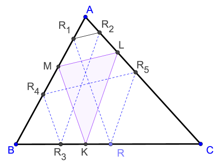
Figure 3: A sub-orthic trajectory example.

In order to show that any sub-orthic trajectory is $2$-gap optimal, we consider a new patrolling problem on input triangle $ABC$ with a limited visitation horizon. In particular, in the $2k$-limited patrolling problem the goal is to find a cyclic trajectory that starts from edge $BC$ (the largest edge) ends after $2k$ visitations of $BC$ and is of minimum total length. Given triangle $ABC$, we denote by $v_{k}$ the cost of the optimal solution to the $2k$-limited patrolling problem. The following is immediate from our definitions.

Observation 6.1

For every $k\geq 1$, the optimal cyclic $2$-gap solution has cost at least $v_{k}/k$.

Now recall that by Lemma 4, any sub-orthic trajectory has $2$-gap cost equal to twice the orthic triangle. Hence, Theorem 3.2 is a corollary of the following lemma.

Lemma 6

The value of  $\lim_{k\rightarrow\infty}v_{k}/k$ equals twice the perimeter of the orthic triangle.

Proof

In order to visualize the $2k$-limited patrolling problem we apply repeatedly ($k$ times) the gadget induced by the reflected triangles of Section 5, see also Figure 4 for an example when $k=2$.

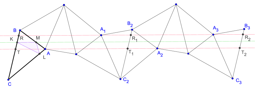
Figure 4: Two applications of reflections.

Indeed, the gadget of the reflected triangles defines $B_{2}C_{2}$ which is parallel to $BC$. One more reflection of $A_{1}$ about $B_{2}C_{2}$ results into triangle $A_{2}B_{2}C_{2}$ whose edges are piecewise parallel to the edges of $ABC$, hence the same reflection sequence, applied on $A_{2}B_{2}C_{2}$ defines $B_{3}C_{3}$ parallel to $B_{2}C_{2}$ and so on.

This way, we define a sequence of parallel segments $B_{k}C_{k}$. Now consider the orthic channel of $ABC$ identified by lines passing through $R,A_{1}$ and $T,A$ (as per Lemma 5). Consider also the corresponding points $R_{k},T_{k}$ that these two lines intersect segments $B_{k}C_{k}$.

By the definition of the $2k$-limited patrolling problem, its optimal schedule (with cost $v_{k}$) is the shortest trajectory that starts from $BC$ and ends at $B_{k}C_{k}$. Since the orthic channel stays within all reflected triangles, the optimal solution to the $2k$-limited patrolling problem is the shortest line segment with endpoints within $RT$ and $R_{k}T_{k}$. Observe that the shortest such segment is the shortest diagonal of parallelogram $RTT_{k}R_{k}$. Now as $k$ grows, one side $RT$ of these parallelograms stays constant, while the length of both diagonals tend (in the limit) to the length of $RR_{k}=TT_{k}$ which are also equal to $k$ times the $2$-gap cost of any sub-orthic trajectory, and hence are equal to $2k$ times the orthic perimeter. ∎

Note that the orthic trajectory is one among the sub-orthic trajectories, and hence optimal too to the $2$-gap patrolling problem (among cyclic algorithms). In the following lemma we show that the orthic trajectory is also the optimal solution to a multi-objective optimization problem.

Lemma 7

Among all $2$-gap optimal sub-orthic trajectories, the one that minimizes the visitation gap between any two (not necessarily same) edges is the orthic trajectory.

Proof

Consider an arbitrary sub-orthic trajectory $RR_{1}R_{2}R_{3}R_{4}R_{5}R$, see Figure 3. Note that the sub-orthic schedule is made up of segments that are piecewise parallel to the segments of the orthic trajectory, and any of the orthic line segments lies in the middle of any of the two parallel segments of the sub-orthic schedule.

In particular we have $RR_{1},R_{3}R_{4}$ are parallel to $MK$, as well as $R_{1}R2,R_{4}R_{5}$ are parallel to $ML$, and $RR_{5},R_{2}R_{3}$ are parallel to $KL$. Moreover, $MK\leq\max\{RR_{1},R_{3}R_{4}\},ML\leq\max\{R_{1}R2,R_{4}R_{5}\}$, and $KL\leq\max\{RR_{5},R_{2}R_{3}\}$. It follows that maximum visitation gap $\max\{MK,ML,KL\}$ between any two edges in the orthic trajectory is at most the maximum visitation gap between any two edges in any sub-orthic trajectory. ∎

7 The $1$-Gap Optimal Schedule

It is immediate from the definitions that half the cost of the $2$-gap optimal patrolling schedule is a lower bound to the cost of the $1$-gap optimal patrolling schedule. By Theorem 3.2, the $2$-gap optimal patrolling schedule has cost 2 times the perimeter of the orthic triangle. Hence, the cost of the $1$-gap optimal schedule is at least the perimeter of the orthic triangle. On the other hand, by Theorem 3.1 we have a patrolling schedule (the orthic trajectory) with $1$-gap cost equal to the orthic perimeter. Therefore, we obtain the following immediate corollary.

Corollary 1

The optimal $1$-gap cyclic schedule of a triangle $\Delta$ is its orthic triangle.

The purpose of this section is to prove Theorem 3.3, that is to strengthen the statement of Corollary 1 by showing that the optimal $1$-gap schedule is actually cyclic. We do so by showing how to modify an arbitrary schedule into a cyclic schedule, without increasing its $1$-gap cost. Effectively, the next lemma implies Theorem 3.3.

Lemma 8

There is a $1$-gap optimal schedule that is cyclic.

Proof

Consider an arbitrary schedule $S=\{s_{i}\}_{i}$ that is not cyclic. We show how to construct a new schedule that is cyclic and 3-periodic, without increasing its $1$-gap. Indeed, since $S$ is not cyclic, and after renaming edges, there are two consecutive visitations of edge $\alpha$ so that both edges $\beta,\gamma$ are visited in between, with at least one of them being visited more than once. In other words, for some $k,\ell\in\mathbb{N}$, $\ell\geq 4$ we have that $e(s_{k})=e(s_{k+\ell})=\alpha$, $e(s_{k+1})=e(s_{k+3})=\beta$ and $e(s_{k+2})=\gamma$.

In what follows we denote by $s_{i}s_{j}$ the distance between points $s_{i},s_{j}$. Then, we see that for the $1$-gap cost $G$ of $S$, we have that

$$G= \max_{\delta\in E}G(\delta)\geq G(\alpha)\geq\sum_{i=0}^{\ell-1}s_{k+i}s_{k+i+1}$$

$$\geq s_{k}s_{k+1}+s_{k+1}s_{k+2}+s_{k+2}s_{k+3}+s_{k+3}s_{k+\ell}$$

$$\geq 2\min\{s_{k}s_{k+1}+s_{k+1}s_{k+2},s_{k+2}s_{k+3}+s_{k+3}s_{k+\ell}\},$$

where the second to last inequality is due to the triangle inequality.

Now we consider two different cyclic and $3$-periodic schedules, $S^{\prime},S^{\prime\prime}$, with $1$-gap costs $G^{\prime},G^{\prime\prime}$, respectively, and we show that $\min\{G^{\prime},G^{\prime\prime}\}\leq G$. The two schedules are the following.

$$S^{\prime} =s_{k},s_{k+1},s_{k+2},s_{k},s_{k+1},s_{k+2},s_{k},s_{k+1},s_{k+2},\ldots$$

$$S^{\prime\prime} =s_{k+2},s_{k+3},s_{k+\ell},s_{k+2},s_{k+3},s_{k+\ell},s_{k+2},s_{k+3},s_{k+\ell},\ldots$$

Since both $S^{\prime},S^{\prime\prime}$ are cyclic and periodic, we have that $G^{\prime}=G^{\prime}(\alpha)=G^{\prime}(\beta)=G^{\prime}(\gamma)$ and $G^{\prime\prime}=G^{\prime\prime}(\alpha)=G^{\prime\prime}(\beta)=G^{\prime\prime}(\gamma)$. In particular, using the triangle inequalities again, we have

$$G^{\prime} =s_{k}s_{k+1}+s_{k+1}s_{k+2}+s_{k+2}s_{k}\leq 2(s_{k}s_{k+1}+s_{k+1}s_{k+2})$$

$$G^{\prime\prime} =s_{k+2}s_{k+3}+s_{k+3}s_{k+\ell}+s_{k+\ell}s_{k+2}\leq 2(s_{k+2}s_{k+3}+s_{k+3}s_{k+\ell}).$$

But then, $\min\{G^{\prime},G^{\prime\prime}\}\leq 2\min\{s_{k}s_{k+1}+s_{k+1}s_{k+2},s_{k+2}s_{k+3}+s_{k+3}s_{k+\ell}\}\leq G$, as wanted. ∎

8 The Greedy Cyclic Algorithm

In this section we prove Theorem 3.4 that is we describe a patrolling schedule that converges to a $3$-periodic cyclic schedule whose $1$-gap cost is off from the $1$-gap optimal cyclic schedule by a factor $\gamma\in[1,1.20711]$. It will follow from our analysis that our greedy algorithm will be nearly optimal for any acute triangle with one arbitrarily small angle, and it will be the worst off from the optimal solution when the given triangle is a right isosceles.

We proceed by the description of a greedy patrolling schedule. We assume that the patroller can remember the current and previously visited edges (not necessarily their points), as well as that it can compute (move along) the projection of its current position to any other edge. Formally, we label the three edges $BC,AB,AC$ as $0,1,2$, respectively. The patrolling schedule starts from an arbitrary point $p_{0}$ on $BC$. For each $i\geq 1$, the patroller moves to point $p_{i}$, which is the projection of $p_{i-1}$ onto edge $i\bmod 3$. Referring to triangle $ABC$ as in Figure 5, we note that the patrolling schedule induces a clockwise cyclic visitation of the given triangle. An immediate corollary of our results will imply that also the corresponding counterclockwise cyclic visitation induces the same $1$-gap cost.

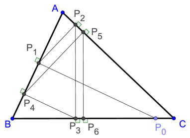
Figure 5: Six iterations of the greedy patrolling schedule that starts from point $p_{0}$ of edge $BC$.

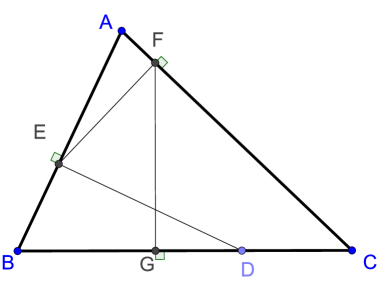
Figure 6: One iteration of the greedy patrolling schedule, stating from point $D$ 1 iteration

Lemma 9

On input acute triangle $ABC$, and for any starting point, the greedy algorithm converges to a cyclic $3$-periodic schedule that has $1$-gap cost

$$p\cdot\frac{\sin(A)\sin(B)\sin(C)}{1+\cos(A)\cos(B)\cos(C)}$$ (3)

where $p$ is the perimeter of triangle $ABC$.

Proof

Consider an arbitrary iteration of the greedy algorithm and a point $D$ on $BC$, see Figure 6. After 3 consecutive steps, the patroller has moved to the projection $E$ of $D$ onto $AB$, its projection $F$ on $AC$ and to its projection $G$ back on $BD$. To simplify calculations, assume also that $AB$ has length $1$. Below, we derive a relation between $BG$ and $BD$.

First we note that $AF=\cos(A)AE=\cos(A)(\gamma-BE)=\cos(A)(\gamma-\cos(B)BD)$. Then, we use the derived formula for $AF$ to calculate

$$BG =1-CG=1-\cos(C)CF=1-\cos(C)(\beta-AF)=1-\cos(C)\left(\beta-\cos(A)(\gamma-\cos(B)BD)\right).$$

It follows that there exists a constant $c$, independent of points $G,D$, such that $BG=c-\cos(A)\cos(B)\cos(C)BD.$ If we denote by $d_{i}$ the distance of a point on the greedy patrolling schedule at the $i$-th visitation of edge $BC$, the previous argument shows that for the same constant $c$, we have $d_{i+1}=c-\cos(A)\cos(B)\cos(C)d_{i}.$

Since $|\cos(A)\cos(B)\cos(C)|<1$, it follows that $\lim_{i\rightarrow\infty}d_{i}$ exists and its value is obtained when in the previous argument points $D,G$ coincide, see Figure 7.

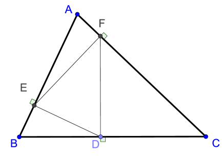
Figure 7: The limiting cyclic $3$-periodic trajectory of the (clockwise) greedy algorithm

We proved that inscribed triangle $DEF$ is the limiting patrolling schedule of the greedy algorithm, which is indeed a cyclic $3$-periodic schedule. Next we calculate its cost. To this end, we claim that triangles $DEF$ and $ABC$ are similar. By denoting by $F,E,G$ the angles of the inscribed triangle, and looking at right triangle $FD$ we have $F=\pi-\pi/2-(\pi-C-\pi/2)=C$. Similarly we obtain that angles $D,B$ are equal, and angles $E,A$ are equal.

Finally we compute the similarity ratio $k<1$ of triangles $DEF,ABC$. We have that

$$\alpha=BD+D\frac{ED}{\sin(B)}+\frac{DF}{\tan(c)}=\frac{k\gamma}{\sin(B)}+\frac{k\alpha}{\tan(C)}=\frac{k\alpha\sin(C)}{\sin(B)}+\frac{k\alpha}{\tan(C)},$$

where the last equality follows from the sin Law in triangle $ABC$. But then, solving for $k$ and simplifying the trigonometric expressions yields $k=\frac{\sin(A)\sin(B)\sin(C)}{1+\cos(A)\cos(B)\cos(C)}.$ It follows that the $1$-gap cost of the induced patrolling schedule is equal to the perimeter of triangle $DEF$ which equals $k$ times the perimeter of $ABC$ as claimed. ∎

We are now ready to prove Theorem 3.4. An immediate corollary of Lemma 9 is that the (limiting) cost of the greedy algorithm is the same also for the corresponding counter-clock wise trajectory. Moreover, the ratio between its cost and the optimal $1$-gap cost, as per Lemma 1, is given by

$$\frac{\sin(A)\sin(B)\sin(C)}{2(1+\cos(A)\cos(B)\cos(C))}\left(\frac{1}{\sin(B)\sin(C)}+\frac{1}{\sin(A)\sin(C)}+\frac{1}{\sin(A)\sin(B)}\right)$$

$$=\frac{\sin(A)+\sin(B)+\sin(C)}{2(1+\cos(A)\cos(B)\cos(C))}.$$

The latter expression, over all non-obtuse triangles, is maximized when any of the angles $A,B,C$ is a right angle, and the other two are equal, that is for the right isosceles, in which case the ratio becomes $\frac{1}{2}\left(\sqrt{2}+1\right)$. In the other extreme case, it is also easy to show that the ratio tends to 1 if any of the angles tends to 0 (hence the other two tend to $\pi/2$), while also for the equilateral triangle, the ratio becomes $2\sqrt{3}/3$.

9 Discussion

In this work we demonstrated the connection between billiard-type trajectories and optimal patrolling schedules in combinatorial optimization. Specifically, we introduced and solved the problem of patrolling the edges of an acute triangle using a unit-speed agent with the goal of minimizing the maximum 1-gap and 2-gap idle time of any edge. We show that billiard-type trajectories are optimal solution to these combinatorial patrolling problems.

Our findings point to several future directions. One natural extension of our work is to generalize the patrolling problem to arbitrary polygons with one or more agents. Moreover, the introduction of the novel 2-gap patrolling problem suggests the investigation of optimal solutions for more complex frequency requirements or time restrictions, especially with the presence of multiple patrolling agents or multiple objects to be patrolled. In that direction, it would be interesting to examine how our results extend to patrolling 3 or more arbitrary line segments on the plane, as subsets of the edges of convex polygones with one or more agents.

References

- [1] A. Almeida, G. Ramalho, H. Santana, P. Azevedo Tedesco, T. Menezes, V. Corruble, and Y. Chevaleyre. Recent advances on multi-agent patrolling. In SBIA, pages 474–483, 2004.
- [2] Steve Alpern, Alec Morton, and Katerina Papadaki. Patrolling games. Oper. Res, 59(5):1246–1257, 2011.
- [3] Nicola Basilico. Recent trends in robotic patrolling. Current Robotics Reports, 3(2):65–76, 2022.
- [4] Andrew M Baxter and Ronald Umble. Periodic orbits for billiards on an equilateral triangle. The American Mathematical Monthly, 115(6):479–491, 2008.
- [5] Nicolas Bedaride. Periodic billiard trajectories in polyhedra. arXiv preprint arXiv:1104.1051, 2011.
- [6] Y. Chevaleyre. Theoretical analysis of the multi-agent patrolling problem. In IAT, pages 302–308, 2004.
- [7] Huda Chuangpishit, Jurek Czyzowicz, Leszek Gasieniec, Konstantinos Georgiou, Tomasz Jurdzinski, and Evangelos Kranakis. Patrolling a path connecting a set of points with unbalanced frequencies of visits. In A Min Tjoa, Ladjel Bellatreche, Stefan Biffl, Jan van Leeuwen, and Jirí Wiedermann, editors, SOFSEM 2018, volume 10706 of Lecture Notes in Computer Science, pages 367–380. Springer, 2018.
- [8] Andrew Collins, Jurek Czyzowicz, Leszek Gasieniec, Adrian Kosowski, Evangelos Kranakis, Danny Krizanc, Russell Martin, and Oscar Morales-Ponce. Optimal patrolling of fragmented boundaries. In Guy E. Blelloch and Berthold Vöcking, editors, 25th ACM Symposium on Parallelism in Algorithms and Architectures, SPAA '13, Montreal, QC, Canada - July 23 - 25, 2013, pages 241–250. ACM, 2013.
- [9] Jurek Czyzowicz, Konstantinos Georgiou, Evangelos Kranakis, Fraser MacQuarrie, and Dominik Pajak. Distributed patrolling with two-speed robots (and an application to transportation). In Begoña Vitoriano and Greg H. Parlier, editors, ICORES (Selected Papers), volume 695 of Communications in Computer and Information Science, pages 71–95, 2016.
- [10] Jurek Czyzowicz, Kostantinos Georgiou, and Evangelos Kranakis. Patrolling. Distributed Computing by Mobile Entities: Current Research in Moving and Computing, pages 371–400, 2019.
- [11] Jurek Czyzowicz, Adrian Kosowski, Evangelos Kranakis, and Najmeh Taleb. Patrolling trees with mobile robots. In Frédéric Cuppens, Lingyu Wang, Nora Cuppens-Boulahia, Nadia Tawbi, and Joaquín García-Alfaro, editors, FPS, volume 10128 of Lecture Notes in Computer Science, pages 331–344. Springer, 2016.
- [12] Peter Damaschke. Two robots patrolling on a line: Integer version and approximability. In Leszek Gasieniec, Ralf Klasing, and Tomasz Radzik, editors, IWOCA, volume 12126 of Lecture Notes in Computer Science, pages 211–223. Springer, 2020.
- [13] Peter Damaschke. Distance-based solution of patrolling problems with individual waiting times. In Matthias Müller-Hannemann and Federico Perea, editors, ATMOS 2021, volume 96 of OASIcs, pages 14:1–14:14. Schloss Dagstuhl - Leibniz-Zentrum für Informatik, 2021.
- [14] Y. Elmaliach, N. Agmon, and G. A. Kaminka. Multi-robot area patrol under frequency constraints. Ann. Math. Artif. Intell., 57(3-4):293–320, 2009.
- [15] Y. Elmaliach, A. Shiloni, and G. A. Kaminka. A realistic model of frequency-based multi-robot polyline patrolling. In AAMAS (1), pages 63–70, 2008.
- [16] Luigi Freda, Mario Gianni, Fiora Pirri, Abel Gawel, Renaud Dubé, Roland Siegwart, and Cesar Cadena. 3d multi-robot patrolling with a two-level coordination strategy. Auton. Robots, 43(7):1747–1779, 2019.
- [17] Ronaldo Garcia. Elliptic billiards and ellipses associated to the 3-periodic orbits. Am. Math. Mon, 126(6):491–504, 2019.
- [18] Tristan Garrec. Continuous patrolling and hiding games. Eur. J. Oper. Res, 277(1):42–51, 2019.
- [19] Konstantinos Georgiou, Somnath Kundu, and Pawel Pralat. Makespan trade-offs for visiting triangle edges - (extended abstract). In Paola Flocchini and Lucia Moura, editors, IWOCA 2021, volume 12757 of Lecture Notes in Computer Science, pages 340–355. Springer, 2021.
- [20] Lorenz Halbeisen and Norbert Hungerbühler. On periodic billiard trajectories in obtuse triangles. SIAM Review, 42(4):657–670, 2000.
- [21] N. Hazon and G. A. Kaminka. On redundancy, efficiency, and robustness in coverage for multiple robots. Robotics and Autonomous Systems, 56(12):1102–1114, 2008.
- [22] Li Huang, MengChu Zhou, Kuangrong Hao, and Edwin S. H. Hou. A survey of multi-robot regular and adversarial patrolling. IEEE CAA J. Autom. Sinica, 6(4):894–903, 2019.
- [23] Roman N Karasev. Periodic billiard trajectories in smooth convex bodies. Geometric and Functional Analysis, 19(2):423–428, 2009.
- [24] Akitoshi Kawamura and Yusuke Kobayashi 0001. Fence patrolling by mobile agents with distinct speeds. Distributed Comput, 28(2):147–154, 2015.
- [25] Akitoshi Kawamura and Makoto Soejima. Simple strategies versus optimal schedules in multi-agent patrolling. Theoretical Computer Science, 839:195–206, 2020.
- [26] Evangelos Kranakis and Danny Krizanc. Optimization problems in infrastructure security. In Foundations and Practice of Security - 8th International Symposium, FPS 2015, Clermont-Ferrand, France, October 26-28, 2015, Revised Selected Papers, pages 3–13, 2015.
- [27] C Lafargue, M Lebental, A Grigis, C Ulysse, I Gozhyk, N Djellali, J Zyss, and S Bittner. Localized lasing modes of triangular organic microlasers. Physical Review E, 90(5):052922, 2014.
- [28] Michel L. Lapidus and Robert G. Niemeyer. Families of periodic orbits of the koch snowflake fractal billiard, 2011.
- [29] Seoung Kyou Lee, Sándor P. Fekete, and James McLurkin. Structured triangulation in multi-robot systems: Coverage, patrolling, voronoi partitions, and geodesic centers. Int. J. Robotics Res, 35(10):1234–1260, 2016.
- [30] A. Machado, G. Ramalho, J.-D. Zucker, and A. Drogoul. Multi-agent patrolling: An empirical analysis of alternative architectures. In MABS, pages 155–170, 2002.
- [31] Oscar Morales-Ponce. Optimal patrolling of high priority segments while visiting the unit interval with a set of mobile robots. In Nandini Mukherjee and Sriram V. Pemmaraju, editors, ICDCN 2020: 21st International Conference on Distributed Computing and Networking, Kolkata, India, January 4-7, 2020, pages 10:1–10:10. ACM, 2020.
- [32] Fabio Pasqualetti, Antonio Franchi, and Francesco Bullo. On optimal cooperative patrolling. In CDC, pages 7153–7158. IEEE, 2010.
- [33] Claudio Piciarelli and Gian Luca Foresti. Drone swarm patrolling with uneven coverage requirements. IET Comput. Vis, 14(7):452–461, 2020.
- [34] David Portugal and Rui P. Rocha. A survey on multi-robot patrolling algorithms. In Luis M. Camarinha-Matos, editor, DoCEIS, volume 349 of IFIP Advances in Information and Communication Technology, pages 139–146. Springer, 2011.
- [35] Richard Evan Schwartz. Obtuse triangular billiards i: Near the (2, 3, 6) triangle. Exp. Math, 15(2):161–182, 2006.
- [36] Richard Evan Schwartz. Obtuse triangular billiards ii: One hundred degrees worth of periodic trajectories. Exp. Math, 18(2):137–171, 2009.
- [37] Xuehou Tan and Bo Jiang 0004. Minimization of the maximum distance between the two guards patrolling a polygonal region. Theor. Comput. Sci, 532:73–79, 2014.
- [38] Serge Troubetzkoy. Dual billiards, fagnano orbits, and regular polygons. Am. Math. Mon, 116(3):251–260, 2009.
- [39] Ya B Vorobets, Gregorii Aleksandrovich Gal'perin, and Anatolii M Stepin. Periodic billiard trajectories in polygons: generating mechanisms. Russian Mathematical Surveys, 47(3):5, 1992.
- [40] V. Yanovski, I. A. Wagner, and A. M. Bruckstein. A distributed ant algorithm for efficiently patrolling a network. Algorithmica, 37(3):165–186, 2003.
- [41] Vladimir Yanovski, Israel A. Wagner, and Alfred M. Bruckstein. A distributed ant algorithm for efficiently patrolling a network. Algorithmica, 37(3):165–186, 2003.