Inference in Experiments with Matched Pairs
and Imperfect Compliance

Abstract

This paper studies inference for the local average treatment effect in randomized controlled trials with imperfect compliance where treatment status is determined according to “matched pairs.” By “matched pairs,” we mean that units are sampled i.i.d. from the population of interest, paired according to observed, baseline covariates and finally, within each pair, one unit is selected at random for treatment. Under weak assumptions governing the quality of the pairings, we first derive the limiting behavior of the usual Wald (i.e., two-stage least squares) estimator of the local average treatment effect. We show further that the conventional heteroskedasticity-robust estimator of its limiting variance is generally conservative in that its limit in probability is (typically strictly) larger than the limiting variance. We therefore provide an alternative estimator of the limiting variance that is consistent for the desired quantity. Finally, we consider the use of additional observed, baseline covariates not used in pairing units to increase the precision with which we can estimate the local average treatment effect. To this end, we derive the limiting behavior of a two-stage least squares estimator of the local average treatment effect which includes both the additional covariates in addition to pair fixed effects, and show that the limiting variance is always less than or equal to that of the Wald estimator. To complete our analysis, we provide a consistent estimator of this limiting variance. A simulation study confirms the practical relevance of our theoretical results. We use our results to revisit a prominent experiment studying the effect of macroinsurance on microenterprise in Egypt.

KEYWORDS: Matched pairs, randomized controlled trial, experiments, noncompliance, imperfect compliance

JEL classification codes: C12, C14

1 Introduction

This paper studies inference for the local average treatment effect in randomized controlled trials with imperfect compliance where treatment status is determined according to “matched pairs.” By “matched pairs,” we mean that units are sampled i.i.d. from the population of interest, paired according to observed, baseline covariates and finally, within each pair, one unit is selected at random for treatment. This method is used routinely in all parts of sciences. Indeed, commands to facilitate its implementation are included in popular software packages, such as sampsi in Stata. References to a variety of specific examples can be found, for instance, in the following surveys of various field experiments: Glennerster and Takavarasha (2014), Riach and Rich (2002), Rosenberger and Lachin (2015). See also Bruhn and McKenzie (2009), who, based on a survey of selected development economists, report that 56% of researchers have used such a design at some point. Furthermore, in many such experiments, compliance may be imperfect: some recent examples of experiments featuring both mathched pairs and imperfect compliance are Groh and McKenzie (2016) and Resnjanskij et al. (2021). Under weak assumptions that ensure pairs are formed so that units within pairs are suitably “close” in terms of observed, baseline covariates, we derive a variety of results pertaining to inference about the local average treatment effect in such experiments.

We first study the behavior of the usual Wald (i.e., two-stage least squares) estimator of the local average treatment effect. When all observed, baseline covariates are used in forming pairs, we find that the estimator is efficient among all estimators for the local average treatment effect in the sense that it achieves the lower bound on the limiting variance developed in Bai et al. (2023b) over a broad class of treatment assignment schemes that hold the marginal probability of treatment assignment equal to one half, thereby including matched pairs, in particular, as a special case. On the other hand, we find that the conventional heteroskedasticity-robust estimator of its limiting variance is conservative in that its limit in probability is always weakly larger than the limiting variance and strictly larger unless heterogeneity is constrained in a particular fashion. We provide an alternative estimator of the limiting variance and show that it is consistent for the desired quantity. In a simulation study, we find that tests using the Wald estimator together with the conventional heteroskedasticity-robust estimator of its limiting variance may as a consequence have very poor power when compared to tests using the Wald estimator together with our estimator of its limiting variance.

Next, we consider situations in which there are additional, observed, baseline covariates that are not used when pairing units. We first derive the limiting behavior for a class of covariate-adjusted estimators indexed by different “working models” for conditional expectations. Importantly, these working models need not be correctly specified for the true conditional expectations in order for this estimator to remain consistent for the local average treatment effect, but we show that the limiting variance of the estimator is minimized, in particular, when they are correctly specified. These results are derived under a high-level assumption governing the quality of the estimators of these working models. We therefore specialize our results for the case of linear working models and characterize the optimal linear working model in the sense of minimizing the limiting variance of the resulting covariate-adjusted estimator among all such working models. We find that this limiting variance can be obtained by a familiar estimator: the two-stage least squares estimator using treatment assignment as an instrument of the coefficient on treatment status in a linear regression of the outcome on the following quantities: treatment status; (functions of) the observed baseline covariates; and pair fixed effects. We complete our analysis by providing an estimator of the limiting variance and show that it is consistent for the desired quantity.

Our paper builds upon the analysis of Bai et al. (2022), who analyzed the behavior of the difference-in-means estimator of the average treatment effect in context of experiments with matched pairs and perfect compliance. Our covariate-adjusted estimator is inspired by the analysis in Bai et al. (2023a), who studied the use of additional, observed, baseline covariates in experiments with matched pairs and perfect compliance to improve the precision with which we can estimate the average treatment effect (similar results have also been obtained by Cytrynbaum, 2023). We emphasize, however, that none of the aforementioned papers permit imperfect compliance, which, as argued by Athey and Imbens (2017), is one of the most common complications in even the most well designed experiments. We note, however, that imperfect compliance has been studied in the context of randomized controlled trials with other treatment assignment schemes, such as stratified block randomization: see, for example, Ansel et al. (2018), Bugni and Gao (2021), and Jiang et al. (2022). We also emphasize that all of these papers, like ours, carry out their analysis in a superpopulation sampling framework. In this way, our analysis differs from the analysis of experiments with a finite population sampling framework.

The remainder of the paper is organized as follows. In Section 2 we describe our setup and notation. In particular, there we describe the precise sense in which we require that units in each pair are “close” in terms of their baseline covariates. Our main results concerning the Wald estimator are contained in Section 3. In Section 4, we develop our results pertaining to our covariate-adjusted estimator that exploits additional observed, baseline covariates not used in pairing units to increase the precision with which we can estimate the local average treatment effect. In Section 5, we examine the practical relevance of our theoretical results via a small simulation study. In Section 6, we provide a brief empirical illustration of our proposed tests using data from an experiment in Groh and McKenzie (2016). Finally, we conclude in Section 7 with some recommendations for empirical practice guided by both our theoretical results and our simulation study. As explained further in that section, we do not recommend the use of the Wald estimator with the conventional heteroskedasticity-robust estimator of its limiting variance because it is conservative in the sense described above; we instead encourage the use of the Wald estimator with our consistent estimator of its limiting variance because it is asymptotically exact, and, as a result, considerably more powerful. When there are additional, observed, baseline covariates that are not used when forming pairs, we recommend the use of our covariate-adjusted Wald estimator with our consistent estimator of its limiting variance. Proofs of all results are provided in the Appendix.

2 Setup and Notation

Let $Y_{i}\in\mathbf{R}$ denote the (observed) outcome of the $i$th unit, $A_{i}\in\{0,1\}$ be an indicator for whether or not unit $i$ is assigned to treatment, $D_{i}\in\{0,1\}$ be an indicator for whether or not unit $i$ decides to take up treatment, $X_{i}\in\mathbf{R}^{k_{x}}$ denote observed, baseline covariates for the $i$th unit which are used for matching, and $W_{i}\in\mathbf{R}^{k_{w}}$ denote observed, baseline covariates for the $i$th unit which will be used when we consider covariate adjustment in Section 4. In contrast to the setting considered in Bai et al. (2022), we allow for imperfect compliance, i.e. for $D_{i}\neq A_{i}$. Further denote by $Y_{i}(d)$ the potential outcome of the $i$th unit if they make treatment decision $d\in\{0,1\}$, and by $D_{i}(a)$ the potential treatment decision of the $i$th unit if assigned to treatment $a\in\{0,1\}$. The observed treatment decision and potential treatment decision are related to treatment assignment via the usual relationship

$$D_{i}=D_{i}(1)A_{i}+D_{i}(0)(1-A_{i})~{},$$ (1)

and the observed outcome and potential outcome are related to treatment decision via the relationship

$$Y_{i}=Y_{i}(1)D_{i}+Y_{i}(0)(1-D_{i})~{}.$$ (2)

We will also often make use of the following alternative representation for the observed outcome, which is numerically equivalent to (2):

$$Y_{i}=\tilde{Y}_{i}(1)A_{i}+\tilde{Y}_{i}(0)(1-A_{i})~{},$$ (3)

where

$$\tilde{Y}_{i}(a)=Y_{i}(1)D_{i}(a)+Y_{i}(0)(1-D_{i}(a))$$ (4)

for $a\in\{0,1\}$. In words, $\tilde{Y}_{i}(a)$ represents the “intent-to-treat” potential outcome for unit $i$ when assigned to treatment $a\in\{0,1\}$.

Following Imbens and Angrist (1994), each participant in the experiment can be categorized into one of four types: units for which $D_{i}(1)=1$ and $D_{i}(0)=0$ are referred to as compliers, units for which $D_{i}(1)=1$ and $D_{i}(0)=1$ are referred to as always takers, units for which $D_{i}(1)=0$ and $D_{i}(0)=0$ are referred to as never takers, and finally units for which $D_{i}(1)=0$ and $D_{i}(0)=1$ are referred to as defiers. We use the notation

$$C_{i}=I\left\{D_{i}(1)=1,D_{i}(0)=0\right\}$$ (5)

below to indicate whether or not unit $i$ is a complier.

For a random variable indexed by $i$, say for example $A_{i}$, it will be useful to denote by $A^{(n)}$ the random vector $(A_{1},...,A_{2n})$. Denote by $P_{n}$ the distribution of the observed data $(Y^{(n)},D^{(n)},A^{(n)},X^{(n)},W^{(n)})$, and by $Q_{n}$ the distribution of $(Y^{(n)}(1),Y^{(n)}(0),D^{(n)}(1),D^{(n)}(0),X^{(n)},W^{(n)})$. Note that $P_{n}$ is jointly determined by (1), (2), $Q_{n}$, and the mechanism for determining treatment assignment. We assume throughout that our sample consists of $2n$ i.i.d. observations, so that $Q_{n}=Q^{2n}$, where $Q$ is the marginal distribution of $(Y_{i}(1),Y_{i}(0),D_{i}(1),D_{i}(0),X_{i},W_{i})$. We therefore state our assumptions below in terms of assumptions on $Q$ and the mechanism for determining treatment assignment. Indeed, we will not make reference to $P_{n}$ in the sequel and all operations are understood to be under $Q$ and the mechanism for determining treatment assignment.

Our object of interest is the local average treatment effect, which may be expressed in our notation as

$$\Delta(Q)=E\left[Y_{i}(1)-Y_{i}(0)|C_{i}=1\right].$$ (6)

For a pre-specified choice of $\Delta_{0}$, the testing problem of interest is

$$H_{0}:\Delta(Q)=\Delta_{0}\ \text{versus}\ H_{1}:\Delta(Q)\neq\Delta_{0}$$ (7)

at level $\alpha\in(0,1)$.

We begin by describing our primary assumptions on the data generating process.

Assumption 2.1.

The distribution $Q$ is such that

1. $0<E\left[\operatorname*{Var}\left[\tilde{Y}_{i}(a)-\Delta(Q)D_{i}(a)|X_{i}\right]\right]$ for $a\in\{0,1\}$.

2. $E\left[Y_{i}(a)^{2}\right]<\infty$ for $a\in\{0,1\}$.

3. $E[Y_{i}(1)^{r}D_{i}(a)|X_{i}=x]$ and $E[Y_{i}(0)^{r}(1-D_{i}(a))|X_{i}=x]$ are Lipschitz for $a=0,1$ and $r=0,1,2$.

4. $P\{D_{i}(1)\geq D_{i}(0)\}=1$.

5. $P\{C_{i}=1\}>0$.

Assumption 2.1(a)–(b) are mild restrictions imposed to rule out degenerate situations and to permit the application of suitable laws of large numbers and central limit theorems. Assumption 2.1(c) is a smoothness requirement that ensures that units that are “close” in terms of their baseline covariates are suitably comparable. Similar smoothness requirements are also considered in Bai et al. (2022), Cytrynbaum (2023), and generally play a key role in establishing the asymptotic exactness of our proposed tests. Assumptions 2.1(d)–(e) are the standard “monotonicity” and “relevance” conditions of Imbens and Angrist (1994) which ensure that the probability limit of the Wald estimator which we define in Section 3 can be interpreted as the local average treatment effect $\Delta(Q)$.

Next, we describe our assumptions on the mechanism determining treatment assignment. Following the notation in Bai et al. (2022), the $n$ pairs can be represented by the sets

$$\{\pi(2j-1),\pi(2j)\}\ \text{for}\ j=1,...,n~{},$$

where $\pi=\pi_{n}\left(X^{(n)}\right)$ is a permutation of $2n$ elements. Given such a $\pi$, we assume that treatment status is assigned as described in the following assumption:

Assumption 2.2.

Treatment status is assigned so that $\left(Y^{(n)}(1),Y^{(n)}(0),D^{(n)}(1),D^{(n)}(0),W^{(n)}\right)\perp\!\!\!\perp A^{(n)}|X^{(n)}$, and conditional on $X^{(n)}$, $(A_{\pi(2j-1)},A_{\pi(2j)})$, $j=1,...,n$ are i.i.d. and each uniformly distributed over the values in $\{(0,1),(1,0)\}$.

We further require that the unts in each pair be “close” in terms of their baseline covariates in the following sense:

Assumption 2.3.

The pairs used in determining treatment status satisfy

$$\frac{1}{n}\sum_{1\leq j\leq n}\|X_{\pi(2j)}-X_{\pi(2j-1)}\|_{2}^{r}\stackrel{{\scriptstyle P}}{{\rightarrow}}0~{},$$

for $r\in\{1,2\}$.

We will also sometimes require that the distances between units in adjacent pairs be “close” in terms of their baseline covariates:

Assumption 2.4.

The pairs used in determining treatment status satisfy

$$\frac{1}{n}\sum_{1\leq j\leq\lfloor\frac{n}{2}\rfloor}\|X_{\pi(4j-k)}-X_{\pi(4j-l)}\|_{2}^{2}\stackrel{{\scriptstyle P}}{{\rightarrow}}0~{},$$

for $k\in\{2,3\}$ and $l\in\{0,1\}$.

Bai et al. (2022) and Bai et al. (2023c) provide several examples of pairing algorithms which satisfy Assumptions 2.3–2.4. The simplest such example is when $X_{i}\in\mathbf{R}$, in which case we can order units from smallest to largest according to $X_{i}$ and pair adjacent units. It then follows from Theorem 4.1 in Bai et al. (2022) that Assumptions 2.3–2.4 are satisfied as long as $E[X_{i}^{2}]<\infty$.

3 Main Results

3.1 Asymptotic Behavior of the Wald Estimator

In this section, we study the asymptotic properties of the standard Wald estimator (i.e., the two-stage least squares estimator of $Y_{i}$ on $D_{i}$ using $A_{i}$ as an instrument) of $\Delta(Q)$ under a matched pairs design. In order to introduce this estimator, define

$$\begin{split}\hat{\psi}_{n}(a)=\frac{1}{n}\sum_{1\leq i\leq 2n:A_{i}=a}Y_{i}~{},\end{split}$$ (8)

$$\begin{split}\hat{\phi}_{n}(a)=\frac{1}{n}\sum_{1\leq i\leq 2n:A_{i}=a}D_{i}~{}.\end{split}$$ (9)

Using this notation, the Wald estimator is defined as

$$\begin{split}\hat{\Delta}_{n}=\frac{\hat{\psi}_{n}(1)-\hat{\psi}_{n}(0)}{\hat{\phi}_{n}(1)-\hat{\phi}_{n}(0)}~{}.\end{split}$$ (10)

Note that this estimator may be obtained as the ratio of the estimator of the coefficient of $A_{i}$ in an ordinary least squares regression of $Y_{i}$ on a constant and $A_{i}$ (the “reduced-form”) to the estimator of the coefficient of $A_{i}$ in an ordinary least squares regression of $D_{i}$ on a constant and $A_{i}$ (the “first-stage”). Theorem 3.1 establishes the limiting distribution of $\hat{\Delta}_{n}$ under a matched pairs design.

Theorem 3.1.

Suppose $Q$ satisfies Assumption 2.1 and the treatment assignment mechanism satisfies Assumptions 2.2–2.3. Then,

$$\sqrt{n}\left(\hat{\Delta}_{n}-\Delta(Q)\right)\stackrel{{\scriptstyle d}}{{\rightarrow}}N\left(0,\nu^{2}\right),$$

where

$$\nu^{2}=\frac{1}{P\{C_{i}=1\}^{2}}\Biggr{(}\operatorname*{Var}[Y^{\ast}_{i}(1)]+\operatorname*{Var}[Y^{\ast}_{i}(0)]\\ -\frac{1}{2}E\left[((E[Y^{\ast}_{i}(1)|X_{i}]-E[Y^{\ast}_{i}(1)])+(E[Y^{\ast}_{i}(0)|X_{i}]-E[Y^{\ast}_{i}(0)]))^{2}\right]\Biggr{)}~{},$$

with

$$Y^{\ast}_{i}(a)=\tilde{Y}_{i}(a)-\Delta(Q)D_{i}(a)~{},$$ (11)

for $a\in\{0,1\}$.

Note that the expression for $\nu^{2}$ corresponds exactly to the limiting variance obtained in Bai et al. (2022) with the usual potential outcomes $Y_{i}(a)$ replaced with the transformed outcomes $Y_{i}^{\ast}(a)$. In particular, when there is perfect compliance, so that $D_{i}=A_{i}$, $P\{C_{i}=1\}=1$, and $D_{i}(a)=a$, the limiting variance we obtain in Theorem 3.1 corresponds exactly to the limiting variance derived in Bai et al. (2022). Moreover, it can be shown that our expression for $\nu^{2}$ attains the efficiency bound derived in Bai et al. (2023b) over a broad class of treatment assignments which include matched pairs as a special case (it can also be shown that this bound coincides with the bounds derived in Frölich, 2007; Hong and Nekipelov, 2010, in settings with observational data with i.i.d assignment when $P\{A_{i}=a|X_{i}\}=1/2$, where the local average treatment effect is estimated non-parametrically using the covariates $X_{i}$: see Lemma A.1 for details.)

Remark 3.1.

It can be shown that under our matched pairs design, the two-stage least squares estimator of $\beta_{1}$ in the linear regression

$$Y_{i}=\beta_{0}+\beta_{1}D_{i}+\gamma^{\prime}X_{i}+\epsilon_{i}~{},$$

with $A_{i}$ used as an instrument for $D_{i}$, is asymptotically equivalent to the Wald estimator $\hat{\Delta}_{n}$. This mirrors similar observations made in Remark 3.8 in Bai et al. (2022) for the case of perfect compliance.   

3.2 Variance Estimation

In this section, we construct a consistent variance estimator for the limiting variance $\nu^{2}$, and then contrast this to the asymptotic behavior of standard regression-based variance estimators. As noted in the discussion following Theorem 3.1, the expression for $\nu^{2}$ corresponds exactly to the limiting variance obtained in Bai et al. (2022) with the usual potential outcomes $Y_{i}(a)$ replaced with the transformed outcomes $Y_{i}^{\ast}(a)$. We thus follow the variance construction from Bai et al. (2022), but with a feasible version of $Y_{i}^{\ast}(a)$ defined as

$$\hat{Y}_{i}=Y_{i}-\hat{\Delta}_{n}D_{i}~{}.$$

This strategy leads to the following variance estimator:

$$\hat{\nu}^{2}_{n}=\frac{\hat{\tau}^{2}_{n}-\frac{1}{2}(\hat{\lambda}^{2}_{n}+\hat{\Gamma}^{2}_{n})}{\left(\hat{\phi}_{n}(1)-\hat{\phi}_{n}(0)\right)^{2}}~{},$$ (12)

where

$$\hat{\tau}^{2}_{n} =\frac{1}{n}\sum_{1\leq j\leq n}(\hat{Y}_{\pi(2j)}-\hat{Y}_{\pi(2j-1)})^{2}$$

$$\hat{\lambda}^{2}_{n} =\frac{2}{n}\sum_{1\leq j\leq\lfloor\frac{n}{2}\rfloor}\left(\hat{Y}_{\pi(4j-3)}-\hat{Y}_{\pi(4j-2)}\right)\left(\hat{Y}_{\pi(4j-1)}-\hat{Y}_{\pi(4j)}\right)\left(A_{\pi(4j-3)}-A_{\pi(4j-2)}\right)\left(A_{\pi(4j-1)}-A_{\pi(4j)}\right)$$

$$\hat{\Gamma}_{n} =\frac{1}{n}\sum_{1\leq i\leq 2n:A_{i}=1}\hat{Y}_{i}-\frac{1}{n}\sum_{1\leq i\leq 2n:A_{i}=0}\hat{Y}_{i}~{}.$$

Note that the construction of the numerator of $\hat{\nu}^{2}_{n}$ can be motivated using a similar intuition to what has been previously discussed in Bai et al. (2022): to consistently estimate

$$E[(E[Y^{\ast}_{i}(1)|X_{i}]-E[Y^{\ast}_{i}(0)|X_{i}])^{2}]~{},$$

ideally we would like access to four different units with similar values of $X_{i}$, of which two are treated. However, because each pair only contains two units, we need to average across “pairs of pairs” of units, where two pairs are grouped together so that they are “close” in terms of $X_{i}$. We establish the following consistency result for $\hat{\nu}^{2}_{n}$:

Theorem 3.2.

Suppose $Q$ satisfies Assumption 2.1 and the treatment assignment mechanism satisfies Assumptions 2.2–2.4. Then,

$$\hat{\nu}_{n}^{2}\stackrel{{\scriptstyle P}}{{\rightarrow}}\nu^{2}.$$

We thus immediately obtain the following corollary which establishes the asymptotic exactness of a $t$-test for the null hypothesis (7) constructed using the variance estimator $\hat{\nu}^{2}_{n}$:

Corollary 3.1.

Suppose $Q$ satisfies Assumption 2.1 and the treatment assignment mechanism satisfies Assumptions 2.2–2.4. Then,

$$\frac{\sqrt{n}\left(\hat{\Delta}_{n}-\Delta(Q)\right)}{\hat{\nu}_{n}}\stackrel{{\scriptstyle d}}{{\rightarrow}}N\left(0,1\right)~{}.$$

Next, we consider the limiting behavior of the usual heteroskedasticity-robust variance estimator from a standard two-stage least squares regression, which is commonly used in practice: see Groh and McKenzie (2016), and Resnjanskij et al. (2021) for examples. Let $\hat{U}_{i}$ denote the $i$th residual generated by the two-stage least squares estimator in a linear regression of $Y_{i}$ on a constant and $D_{i}$ using $A_{i}$ as an instrument for $D_{i}$. The heteroskedasticity-robust variance estimator is defined as

$$\hat{\omega}_{n}^{2}=\left(n\left(\sum_{1\leq i\leq 2n}\begin{pmatrix}1\\ A_{i}\end{pmatrix}\begin{pmatrix}1&D_{i}\end{pmatrix}\right)^{-1}\sum_{1\leq i\leq 2n}\hat{U}_{i}^{2}\begin{pmatrix}1\\ A_{i}\end{pmatrix}\begin{pmatrix}1&A_{i}\end{pmatrix}\left(\sum_{1\leq i\leq 2n}\begin{pmatrix}1\\ D_{i}\end{pmatrix}\begin{pmatrix}1&A_{i}\end{pmatrix}\right)^{-1}\right)_{2,2}~{},$$ (13)

where the notation $(\cdot)_{2,2}$ denotes the $(2,2)$-element of its (matrix) argument. Theorem 3.3 derives the limit in probability of $\hat{\omega}_{n}^{2}$.

Theorem 3.3.

Suppose $Q$ satisfies Assumption 2.1 and the treatment assignment mechanism satisfies Assumptions 2.2–2.3. Then,

$$\hat{\omega}_{n}^{2}\stackrel{{\scriptstyle P}}{{\rightarrow}}\omega^{2}~{},$$

where

$$\omega^{2}=\frac{1}{P\{C_{i}=1\}^{2}}(\operatorname*{Var}[Y_{i}^{\ast}(1)]+\operatorname*{Var}[Y_{i}^{\ast}(0)])~{}.$$

We thus immediately obtain the following corollary which establishes the conservativness of a $t$-test constructed using the variance estimator $\hat{\omega}_{n}^{2}$ for the null hypothesis (7).

Corollary 3.2.

Suppose $Q$ satisfies Assumption 2.1 and the treatment assignment mechanism satisfies Assumptions 2.2–2.3. Then,

$$\frac{\sqrt{n}\left(\hat{\Delta}_{n}-\Delta(Q)\right)}{\hat{\omega}_{n}}\stackrel{{\scriptstyle d}}{{\rightarrow}}N\left(0,\xi^{2}\right),$$

where $\xi^{2}\leq 1$ and the inequality is strict unless

$$E[\tilde{Y}_{i}(1)-\Delta(Q)D_{i}(1)+\tilde{Y}_{i}(0)-\Delta(Q)D_{i}(0)|X_{i}]=E[\tilde{Y}_{i}(1)-\Delta(Q)D_{i}(1)+\tilde{Y}_{i}(0)-\Delta(Q)D_{i}(0)]$$

with probability one under $Q$.

4 Covariate Adjustment

In this section, we consider a generalization of the estimator $\hat{\Delta}_{n}$ defined in Section 3.1 that allows for covariate adjustment using the additional, observed, baseline covariates $W^{(n)}$ that are not used when forming pairs. We then show how a careful application of this covariate-adjusted estimator can ensure an improvement over the unadjusted Wald estimator $\hat{\Delta}_{n}$ in terms of precision.

Following Bai et al. (2023a), note that it can be shown under Assumption 2.2 that for any $a\in\{0,1\}$, $m_{a,\tilde{Y}}:\mathbb{R}^{k_{x}}\times\mathbb{R}^{k_{w}}\to\mathbb{R}$, and $m_{a,D}:\mathbb{R}^{k_{x}}\times\mathbb{R}^{k_{w}}\to\mathbb{R}$ such that $E[|m_{a,\tilde{Y}}(X_{i},W_{i})|]<\infty$, $E[|m_{a,D}(X_{i},W_{i})|]<\infty$,

$$E[2I\left\{A_{i}=a\right\}(Y_{i}-m_{a,\tilde{Y}}(X_{i},W_{i}))+m_{a,\tilde{Y}}\left(X_{i},W_{i}\right)]=E[\tilde{Y}_{i}(a)],$$ (14)

$$E\left[2I\left\{A_{i}=a\right\}\left(D_{i}-m_{a,D}\left(X_{i},W_{i}\right)\right)+m_{a,D}\left(X_{i},W_{i}\right)\right]=E\left[D_{i}(a)\right].$$ (15)

Here, we view $m_{a,D}$ and $m_{a,\tilde{Y}}$ as “working models” of $E[\tilde{Y}_{i}(a)|X_{i},W_{i}]$ and $E[D_{i}(a)|X_{i},W_{i}]$, respectively, but we emphasize that (14)–(15) hold even if they are incorrectly specified. This observation suggests a covariate-adjusted estimator defined as

$$\hat{\Delta}_{n}^{\rm adj}=\frac{\hat{\psi}_{n}^{\rm adj}(1)-\hat{\psi}_{n}^{\rm adj}(0)}{\hat{\phi}_{n}^{\rm adj}(1)-\hat{\phi}_{n}^{\rm adj}(0)}~{},$$

where

$$\hat{\psi}_{n}^{\rm adj}(a) =\frac{1}{2n}\sum_{1\leq i\leq 2n}(2I\{A_{i}=a\}(Y_{i}-\hat{m}_{a,\tilde{Y}}(X_{i},W_{i}))+\hat{m}_{a,\tilde{Y}}(X_{i},W_{i}))~{},$$

$$\hat{\phi}_{n}^{\rm adj}(a) =\frac{1}{2n}\sum_{1\leq i\leq 2n}(2I\{A_{i}=a\}(D_{i}-\hat{m}_{a,D}(X_{i},W_{i}))+\hat{m}_{a,D}(X_{i},W_{i}))~{},$$

and $\hat{m}_{a,\tilde{Y}}$ and $\hat{m}_{a,D}$ are suitable estimators of $m_{a,\tilde{Y}}$ and $m_{a,D}$. Note that if we set $\hat{m}_{a,\tilde{Y}}=\hat{m}_{a,D}=0$, then $\hat{\Delta}_{n}^{\rm adj}$ simplifies to $\hat{\Delta}_{n}$. Theorem 4.1 below establishes the limiting distribution of $\hat{\Delta}_{n}^{\rm adj}$ for a matched-pairs design under the following high-level assumption on the working models:

Assumption 4.1.

Let $m_{a,\tilde{Y}D}=m_{a,\tilde{Y}}-\Delta(Q)m_{a,D}$. The functions $m_{a,\tilde{Y}D}$ for $a\in\{0,1\}$ satisfy

1. For $a\in\{0,1\}$,

   $$\lim_{\lambda\to\infty}E\left[m_{a,\tilde{Y}D}(X_{i},W_{i})^{2}I\left\{|m_{a,\tilde{Y}D}(X_{i},W_{i})|>\lambda\right\}\right]=0~{}.$$

2. $E[m_{a,\tilde{Y}D}(X_{i},W_{i})|X_{i}=x]$, $E[(m_{a,\tilde{Y}D}(X_{i},W_{i}))^{2}|X_{i}=x]$, and $E[m_{a,\tilde{Y}D}(X_{i},W_{i})Y_{i}^{\ast}(a)|X_{i}=x]$ for $d\in\{0,1\}$, and $E[m_{1,\tilde{Y}D}(X_{i},W_{i})m_{0,\tilde{Y}D}(X_{i},W_{i})|X_{i}=x]$ are Lipschitz.

Before proceeding, we note that we later provide low-level sufficient conditions for this high-level assumption for the special case in which $m_{a,\tilde{Y}}$ and $m_{a,D}$ correspond to linear working models that are optimal in the sense of minimizing the limiting variance of $\hat{\Delta}_{n}^{\rm adj}$ among all linear working models.

Theorem 4.1.

Suppose $Q$ satisfies Assumption 2.1, the treatment assignment mechanism satisfies Assumptions 2.2–2.3, and $m_{a,\tilde{Y}}$ and $m_{a,D}$ for $a\in\{0,1\}$ satisfy Assumption 4.1. Further suppose $\hat{m}_{a,\tilde{Y}}$ and $\hat{m}_{a,D}$ satisfy that

$$\frac{1}{\sqrt{2n}}\sum_{1\leq i\leq 2n}(2A_{i}-1)(\hat{m}_{a,\tilde{Y}}(X_{i},W_{i})-m_{a,\tilde{Y}}(X_{i},W_{i}))\stackrel{{\scriptstyle P}}{{\rightarrow}}0~{},$$ (16)

$$\frac{1}{\sqrt{2n}}\sum_{1\leq i\leq 2n}(2A_{i}-1)(\hat{m}_{a,D}(X_{i},W_{i})-m_{a,D}(X_{i},W_{i}))\stackrel{{\scriptstyle P}}{{\rightarrow}}0~{}.$$ (17)

Then, $\hat{\Delta}_{n}^{\rm adj}$ satisfies

$$\sqrt{n}\left(\hat{\Delta}_{n}^{\rm adj}-\Delta(Q)\right)\stackrel{{\scriptstyle d}}{{\rightarrow}}N\left(0,\nu_{\rm adj}^{2}\right),$$

where $\nu_{\rm adj}^{2}=\frac{1}{P\{C_{i}=1\}^{2}}(\nu_{1,\rm adj}^{2}+\nu_{2,\rm adj}^{2}+\nu_{3,\rm adj}^{2})$ with

$$\nu_{1,\rm adj}^{2} =\frac{1}{2}E[\operatorname*{Var}[E\left[Y_{i}^{\ast}(1)+Y_{i}^{\ast}(0)|X_{i},W_{i}\right]-(m_{1,\tilde{Y}D}(X_{i},W_{i})+m_{0,\tilde{Y}D}(X_{i},W_{i}))|X_{i}]]~{},$$

$$\nu_{2,\rm adj}^{2} =\frac{1}{2}\operatorname*{Var}[E[Y^{\ast}_{i}(1)-Y^{\ast}_{i}(0)|X_{i},W_{i}]]~{},$$

$$\nu_{3,\rm adj}^{2} =E[\operatorname*{Var}[Y^{\ast}_{i}(1)|X_{i},W_{i}]+\operatorname*{Var}[Y^{\ast}_{i}(0)|X_{i},W_{i}]]~{}.$$

Note that the expression for $\nu_{\rm adj}^{2}$ corresponds exactly to the limiting variance obtained in Bai et al. (2023a) with the usual potential outcomes $Y_{i}(a)$ replaced with the transformed outcomes $Y_{i}^{\ast}(a)$ and the working models in Bai et al. (2023a) replaced with $m_{a,\tilde{Y}}(X_{i},W_{i})-\Delta(Q)m_{a,D}(X_{i},W_{i})$. In general, $\nu^{2}_{\rm adj}$ is not guaranteed to be weakly smaller than $\nu^{2}$ for all choices of working models, but we note that $\nu_{\rm adj}^{2}$ is minimized when $\nu_{1,\rm adj}^{2}=0$, i.e., when the working models satisfy

$$E[Y_{i}^{\ast}(1)+Y_{i}^{\ast}(0)|X_{i},W_{i}]-E[Y_{i}^{\ast}(1)+Y_{i}^{\ast}(0)|X_{i}]\\ =m_{1,\tilde{Y}D}(X_{i},W_{i})+m_{0,\tilde{Y}D}(X_{i},W_{i})-E[m_{1,\tilde{Y}D}(X_{i},W_{i})+m_{0,\tilde{Y}D}(X_{i},W_{i})|X_{i}]$$

with probability one. This property holds, in particular, when $m_{a,\tilde{Y}}$ and $m_{a,D}$ are correctly specified.

We now specialize Theorem 4.1 to the case in which $m_{a,\tilde{Y}}$ and $m_{a,D}$ are the optimal linear working models in a sense to be described below. To that end, let $\zeta_{i}=\zeta(X_{i},W_{i})$ be a user-specified transformation of the baseline characteristics $(X_{i},W_{i})$ given by some function $\zeta:\mathbb{R}^{k_{x}}\times\mathbb{R}^{k_{w}}\to\mathbb{R}^{p}$. Denote by $\hat{\beta}_{n}^{Y}$ and $\hat{\beta}_{n}^{D}$ the ordinary least squares estimators of $\beta^{Y}$ and $\beta^{D}$ in the following two linear regressions with pair fixed effects:

$$Y_{i} =\alpha^{Y}A_{i}+\zeta_{i}^{\prime}\beta^{Y}+\sum_{1\leq j\leq n}\theta_{j}^{Y}I\{i\in\{\pi(2j-1),\pi(2j)\}\}+\epsilon_{i}^{Y}$$ (18)

$$D_{i} =\alpha^{D}A_{i}+\zeta_{i}^{\prime}\beta^{D}+\sum_{1\leq j\leq n}\theta_{j}^{D}I\{i\in\{\pi(2j-1),\pi(2j)\}\}+\epsilon_{i}^{D}$$ (19)

Using this notation, consider $\hat{\Delta}^{\rm adj}_{n}$ with $\hat{m}_{a,\tilde{Y}}(X_{i},W_{i})=\zeta_{i}^{\prime}\hat{\beta}_{n}^{Y}$ and $\hat{m}_{a,D}(X_{i},W_{i})=\zeta_{i}^{\prime}\hat{\beta}_{n}^{D}$ for $a\in\{0,1\}$. In order to analyze the large-sample behavior of this estimator, we introduce the following assumption:

Assumption 4.2.

The function $\zeta(\cdot)$ is such that

1. No component of $\zeta_{i}$ is a constant and $E[\operatorname*{Var}[\zeta_{i}|X_{i}]]$ is nonsingular.

2. $\operatorname*{Var}[\zeta_{i}]<\infty$.

3. $E[\zeta_{i}|X_{i}=x]$, $E[\zeta_{i}\zeta_{i}^{\prime}|X_{i}=x]$, $E[\zeta_{i}\tilde{Y}_{i}(a)|X_{i}=x]$, $E[\zeta_{i}D_{i}(a)|X_{i}=x]$ are Lipschitz.

Theorem 4.2 shows that Assumption 4.2 provides low-level sufficient conditions for Assumption 4.1. In this way, it establishes the large-sample behavior of $\hat{\Delta}_{n}^{\rm adj}$ for the special case of these working models and further verifies their optimality among all linear working models:

Theorem 4.2.

Suppose $Q$ satisfies Assumption 2.1, the treatment assignment mechanism satisfies Assumptions 2.2–2.3, and in addition Assumption 4.2 is satisfied. Then,

$$\hat{\beta}_{n}^{Y} \stackrel{{\scriptstyle P}}{{\to}}\beta^{\tilde{Y}}=(2E[\operatorname*{Var}[\zeta_{i}|X_{i}]])^{-1}E[\operatorname*{Cov}[\zeta_{i},\tilde{Y}_{i}(1)+\tilde{Y}_{i}(0)|X_{i}]]$$

$$\hat{\beta}_{n}^{D} \stackrel{{\scriptstyle P}}{{\to}}\beta^{D}=(2E[\operatorname*{Var}[\zeta_{i}|X_{i}]])^{-1}E[\operatorname*{Cov}[\zeta_{i},D_{i}(1)+D_{i}(0)|X_{i}]]~{}.$$

In addition, (16)–(17) and Assumption 4.1 are satisfied for $\hat{m}_{a,\tilde{Y}}(X_{i},W_{i})=\zeta_{i}^{\prime}\hat{\beta}_{n}^{Y}$, $\hat{m}_{a,D}(X_{i},W_{i})=\zeta_{i}^{\prime}\hat{\beta}_{n}^{D}$, $m_{1,\tilde{Y}}(X_{i},W_{i})=m_{0,\tilde{Y}}(X_{i},W_{i})=\zeta_{i}^{\prime}\beta^{\tilde{Y}}$, and $m_{1,\tilde{D}}(X_{i},W_{i})=m_{0,\tilde{D}}(X_{i},W_{i})=\zeta_{i}^{\prime}\beta^{D}$. Moreover, $\hat{\Delta}_{n}^{\rm adj}$ is optimal in the sense of minimizing $\nu_{\rm adj}^{2}$ among all choices of $m_{a,D}$ and $m_{a,\tilde{Y}}$ that are linear in $\zeta_{i}$.

Remark 4.1.

Here, we present two equivalent expressions for $\hat{\Delta}^{\rm adj}_{n}$ when $\hat{m}_{a,\tilde{Y}}(X_{i},W_{i})=\zeta_{i}^{\prime}\hat{\beta}_{n}^{Y}$ and $\hat{m}_{a,D}(X_{i},W_{i})=\zeta_{i}^{\prime}\hat{\beta}_{n}^{D}$. Denote by $\hat{\alpha}_{n}^{Y}$ and $\hat{\alpha}_{n}^{D}$ the ordinary least squares estimators of $\alpha^{Y}$ and $\alpha^{D}$ in (18)–(19). The Frisch-Waugh-Lovell theorem implies that

$$\hat{\alpha}_{n}^{Y} = \hat{\psi}_{n}^{\rm adj}(1)-\hat{\psi}_{n}^{\rm adj}(0)$$

$$\hat{\alpha}_{n}^{D} = \hat{\phi}_{n}^{\rm adj}(1)-\hat{\phi}_{n}^{\rm adj}(0)~{}.$$

It thus follows immediately that

$$\hat{\Delta}_{n}^{\rm adj}=\frac{\hat{\alpha}_{n}^{Y}}{\hat{\alpha}_{n}^{D}}~{}.$$

Next, denote by $\hat{\alpha}_{n}^{\rm IV}$ estimator of $\alpha$ in the following linear regression

$$Y_{i}=\alpha D_{i}+\zeta_{i}^{\prime}\beta+\sum_{1\leq j\leq n}\theta_{j}I\{i\in\{\pi(2j-1),\pi(2j)\}\}+\epsilon_{i}~{}.$$ (20)

obtained by applying two-stage least squares with $A_{i}$ as an instrument for $D_{i}$. It can be shown that

$$\hat{\Delta}_{n}^{\rm adj}=\hat{\alpha}_{n}^{\rm IV}~{}.$$

See Appendix B for details. We emphasize, however, that the usual heteroskedasticity-robust estimator of the variance of $\hat{\alpha}_{n}^{\rm IV}$ is not consistent for the limiting variance derived in Theorem 4.1; Bai et al. (2023c) provide a related discussion of when such an estimator may even be invalid. We therefore construct a consistent estimator of the required variance in Theorem 4.3 below.   

Finally, we construct a consistent variance estimator for the limiting variance $\nu_{\rm adj}^{2}$. As noted in the discussion following Theorem 4.1, the expression for $\nu_{\rm adj}^{2}$ corresponds exactly to the limiting variance obtained in Bai et al. (2023a) with the usual potential outcomes $Y_{i}(a)$ replaced with the transformed outcomes $Y_{i}^{\ast}(a)$ and working models in Bai et al. (2023a) replaced with $m_{a,\tilde{Y}}(X_{i},W_{i})-\Delta(Q)m_{a,D}(X_{i},W_{i})$. We thus follow the variance construction from Bai et al. (2023a), but with a feasible version of $Y_{i}^{\ast}(a)$ defined as

$$\hat{Y}_{i}=Y_{i}-\hat{\Delta}_{n}D_{i}~{},$$

and a feasible version of $m_{a,\tilde{Y}}(X_{i},W_{i})-\Delta(Q)m_{a,D}(X_{i},W_{i})$ defined as

$$\hat{m}_{a,\tilde{Y}D}(X_{i},W_{i})=\hat{m}_{a,\tilde{Y}}(X_{i},W_{i})-\hat{\Delta}_{n}\hat{m}_{a,D}(X_{i},W_{i})~{}.$$

This strategy leads to the following variance estimator:

$$\hat{\nu}_{n,\rm adj}^{2}=\frac{\hat{\tau}_{n,\rm adj}^{2}-\frac{1}{2}(\hat{\lambda}_{n,\rm adj}+\hat{\Gamma}_{n,\rm adj}^{2})}{(\hat{\phi}_{n}^{\rm adj}(1)-\hat{\phi}_{n}^{\rm adj}(0))^{2}}~{},$$ (21)

where

$$\hat{\tau}_{n,\rm adj}^{2} =\frac{1}{n}\sum_{1\leq j\leq n}(\hat{Y}_{\pi(2j-1),\rm adj}-\hat{Y}_{\pi(2j),\rm adj})^{2}~{},$$

$$\hat{\lambda}_{n,\rm adj} =\frac{2}{n}\sum_{1\leq j\leq\lfloor\frac{n}{2}\rfloor}(\hat{Y}_{\pi(4j-3),\rm adj}-\hat{Y}_{\pi(4j-2),\rm adj})$$

$$\hskip 30.00005pt\times(\hat{Y}_{\pi(4j-1),\rm adj}-\hat{Y}_{\pi(4j),\rm adj})(A_{\pi(4j-3)}-A_{\pi(4j-2)})(A_{\pi(4j-1)}-A_{\pi(4j)})~{},$$

$$\hat{\Gamma}_{n,\rm adj} =\frac{1}{n}\sum_{1\leq i\leq n:A_{i}=1}\hat{Y}_{i,\rm adj}-\frac{1}{n}\sum_{1\leq i\leq n:A_{i}=0}\hat{Y}_{i,\rm adj}~{},$$

$$\hat{Y}_{i,\rm adj} =\hat{Y}_{i}-\frac{1}{2}(\hat{m}_{1,\tilde{Y}D}(X_{i},W_{i})+\hat{m}_{0,\tilde{Y}D}(X_{i},W_{i}))~{}.$$

The following theorem establishes the consistency of $\hat{\nu}_{n,\rm adj}^{2}$ for $\nu_{\rm adj}^{2}$:

Theorem 4.3.

Suppose $Q$ satisfies Assumption 2.1, the treatment assignment mechanism satisfies Assumptions 2.2–2.4, and $m_{a,\tilde{Y}}$ and $m_{a,D}$ for $a\in\{0,1\}$ satisfy Assumption 4.1. Further suppose $\hat{m}_{a,\tilde{Y}}$ and $\hat{m}_{a,D}$ satisfy (16)–(17) and

$$\frac{1}{2n}\sum_{1\leq i\leq 2n}(\hat{m}_{a,\tilde{Y}}(X_{i},W_{i})-m_{a,\tilde{Y}}(X_{i},W_{i}))^{2}\stackrel{{\scriptstyle P}}{{\rightarrow}}0~{},$$ (22)

$$\frac{1}{2n}\sum_{1\leq i\leq 2n}(\hat{m}_{a,D}(X_{i},W_{i})-m_{a,D}(X_{i},W_{i}))^{2}\stackrel{{\scriptstyle P}}{{\rightarrow}}0~{}.$$ (23)

Then,

$$\hat{\nu}_{n,\rm adj}^{2}\stackrel{{\scriptstyle P}}{{\rightarrow}}\nu_{\rm adj}^{2}~{}.$$

5 Simulations

In this section, we examine the finite-sample behavior of the estimation and inference procedures introduced in Section 3. Following the simulation design in Bai et al. (2022), the potential outcomes are generated according to the equation:

$$Y_{i}(d)=\mu_{d}+m_{d}(X_{i})+\sigma_{d}(X_{i})\epsilon_{d,i},$$

where $\mu_{d}$, $m_{d}(X_{i})$, and $\epsilon_{d,i}$ are specified in each model below. In Models 1–3, we model compliance status as being independent of potential outcomes and covariates, with each of the following three compliance types being equally likely: compliers, always takers, and never takers. In Models 4–6, we allow the compliance status of an individual to depend on $X_{i}$, and define $C_{i}=1$ if individual $i$ is a complier, $AT_{i}=1$ if individual $i$ is an always taker, and $NT_{i}=1$ if individual $i$ is a never taker. We consider the following model specifications:

• • • $X_{i}\sim\text{Unif}[0,1]$; $m_{1}(X_{i})=m_{0}(X_{i})=\gamma(X_{i}-\frac{1}{2})$; $\epsilon_{d,i}\sim N(0,1)$ for $d\in\{0,1\}$; $\sigma_{0}(X_{i})=\sigma_{0}=1$, and $\sigma_{1}(X_{i})=\sigma_{1}$. $\gamma=1$, $\sigma_{1}=1$, $\mu_{0}=0$ and $\mu_{1}=\Delta$, where $\Delta=0$ is to study the behavior of the tests under the null hypothesis and $\Delta=1$ is to study the behavior of the tests under the alternative hypothesis.

    • As in Model 1, but $m_{0}(X_{i})=0$, and $m_{1}(X_{i})=10\left(X_{i}^{2}-\frac{1}{3}\right)$.

    • As in Model 2, but $\sigma_{0}(X_{i})=X_{i}^{2}$ and $\sigma_{1}(X_{i})=\sigma_{1}X_{i}^{2}$.

    • As in Model 1, but $P\{C_{i}=1|X_{i}\}=X_{i}$, and $P\{AT_{i}=1|X_{i}\}=P\{NT_{i}=1|X_{i}\}=\frac{1-X_{i}}{2}$.

    • As in Model 4, but $m_{0}(X_{i})=0$, and $m_{1}(X_{i})=10\left(X_{i}^{2}-\frac{1}{3}-\frac{1}{6}\right)$.

    • As in Model 5, but $\sigma_{0}(X_{i})=X_{i}^{2}$ and $\sigma_{1}(X_{i})=\sigma_{1}X_{i}^{2}$.

Since $\dim(X_{i})=1$, we construct pairs by sorting units according to $X_{i}$ and matching adjacent units. By Theorem 4.1 in Bai et al. (2022), this pairing algorithm ensures that both Assumptions 2.3 and 2.4 are satisfied. Table 1 reports the rejection probabilities from $5000$ Monte Carlo replications, for testing the null hypothesis (7) using $t$-tests constructed using either the regression-based variance $\hat{\omega}_{n}^{2}$ (Robust and Robust-S, where Robust-S employs a standard small sample correction) or the consistent estimator $\hat{\nu}^{2}_{n}$ (MPIV). As expected given our theoretical results, the regression-based estimator $\hat{\omega}_{n}^{2}$ is conservative, which leads to a loss of power relative to our consistent estimator $\hat{\nu}^{2}_{n}$. Figure 1 displays the power curves for Models 1–6 with $2n=1000$.

		$H_{0}:\Delta=0$			$H_{1}:\Delta=1$
Model	Sample Size	Robust	Robust-S	MPIV	Robust	Robust-S	MPIV
1	200	2.72	2.64	3.36	60.76	60.46	63.36
	800	4.10	4.06	5.10	99.14	99.14	99.38
	1600	4.22	4.20	4.98	100.00	100.00	100.00
	3200	4.42	4.38	5.10	100.00	100.00	100.00
2	200	0.48	0.46	3.50	10.60	10.34	25.80
	800	0.78	0.78	4.50	53.28	53.20	73.70
	1600	1.30	1.30	5.00	87.20	87.16	95.10
	3200	1.14	1.14	5.14	99.52	99.52	99.96
3	200	0.36	0.34	3.14	11.46	11.14	33.50
	800	0.34	0.34	4.44	61.84	61.72	85.04
	1600	0.76	0.74	5.04	93.24	93.20	98.62
	3200	0.72	0.72	5.16	99.94	99.94	100.00
4	200	3.58	3.46	4.56	91.64	91.52	92.58
	800	4.10	4.08	4.96	100.00	100.00	100.00
	1600	4.06	4.06	5.04	100.00	100.00	100.00
	3200	4.00	4.00	4.84	100.00	100.00	100.00
5	200	1.36	1.30	4.80	20.80	20.42	41.58
	800	1.36	1.36	4.60	90.24	90.16	96.90
	1600	1.58	1.56	4.72	99.80	99.80	99.98
	3200	1.32	1.32	4.82	100.00	100.00	100.00
6	200	1.02	0.98	4.86	23.64	23.20	52.04
	800	0.94	0.92	4.94	95.70	95.70	99.48
	1600	1.02	1.02	5.20	100.00	100.00	100.00
	3200	0.78	0.78	4.38	100.00	100.00	100.00

Table 1: Rejection rates for Models 1, 2, 3, 4, 5, and 6

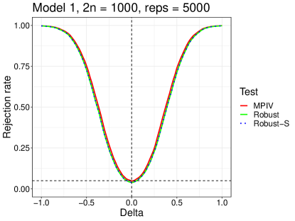
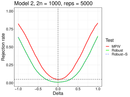
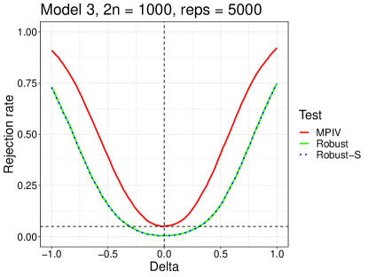
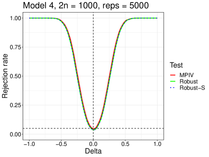
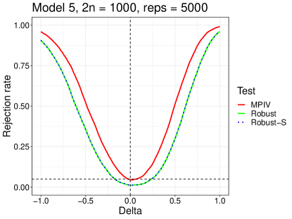
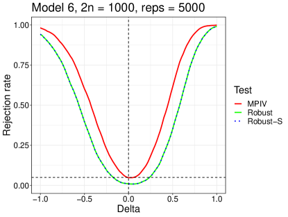
Figure 1: Power Curves

6 Empirical Application

In this section, we illustrate our findings by revisiting the empirical application in Groh and McKenzie (2016). Groh and McKenzie (2016) designed a matched-pair experiment in Egypt to study the effect on microenterprises of acquiring insurance against macroeconomic shocks. The eligibility to purchase macroinsurance was offered to companies in the treatment group. The take-up rate of purchasing in the treatment group was 37%: among 1481 companies in the treatment group, 548 of them purchased insurance. We also note among 1480 companies in the control group, 5 of them purchased insurance as well.

Table 2 reports the estimated LATEs for a collection of outcomes, using both the unadjusted Wald estimator $\hat{\Delta}_{n}$ as well as the linearly adjusted estimator $\hat{\Delta}_{n}^{\rm adj}$ which uses the same covariates as those considered in the analysis in Groh and McKenzie (2016). We also report the standard errors obtained from the regression-based variance estimator $\hat{\omega}_{n}^{2}$ as well as the standard errors obtained from our consistent variance estimators $\hat{\nu}^{2}_{n}$ and $\hat{\nu}^{2}_{n,\rm adj}$ (note that we do not report the standard error obtained from the standard regression-based variance estimator when considering covariate adjustment, since as mentioned in Remark 4.1 this is not guaranteed to be valid). Our findings are consistent with the theoretical results presented in Sections 3 and 4: for the unadjusted estimates, standard errors constructed from $\hat{\nu}^{2}_{n}$ are smaller than those constructed from $\hat{\omega}^{2}_{n}$ across all outcomes, and in fact result in significance tests for the effect on profits and the aggregate index which reject at the $10\%$ level. For the adjusted estimates, we find that the standard errors constructed from $\hat{\nu}^{2}_{n,\rm adj}$ are smaller than those constructed from $\hat{\nu}^{2}_{n}$ across all outcomes. However, point estimates for profits and the aggregate index change in such a way that these are no longer significant at the $10\%$ level.

Table 2: Summary of Estimates Obtained from Empirical Application Groh and McKenzie (2016)

High High Number Any Owner’s Monthly Aggregate Profits Profit Revenue Revenue Employees Worker Hours Consumption Index $\hat{\Delta}_{n}$ -241.602 -0.029 -2561.536 -0.063 -0.085 0.009 -1.324 -14.197 -0.104 SE from $\hat{\omega}^{2}_{n}$ (149.696) (0.022) (937.455)^∗∗∗ (0.021)^∗∗∗ (0.144) (0.050) (2.506) (91.237) (0.069) SE from $\hat{\nu}^{2}_{n}$ (130.946)^∗ (0.021) (841.562)^∗∗∗ (0.020)^∗∗∗ (0.138) (0.049) (2.179) (79.273) (0.061)^∗ $\hat{\Delta}_{n}^{\rm adj}$ -151.345 -0.020 -1802.829 -0.052 -0.023 0.024 -0.401 6.541 -0.069 SE from $\hat{\nu}^{2}_{n,\rm adj}$ (120.969) (0.020) (751.651)^∗∗ (0.018)^∗∗∗ (0.133) (0.047) (2.116) (74.388) (0.057) Sample Size 2804 2804 2800 2800 2824 2824 2796 2880 2880

• Notes: ^∗: significant at 10% level. ^∗∗: significant at 5% level. ^∗∗∗: significant at 1% level. For each outcome listed in Table 7 of Groh and McKenzie (2016), we report (a) the Wald estimates $\hat{\Delta}_{n}$ in (10), (b) the robust standard error obtained from $\hat{\omega}^{2}_{n}$ in (13), (c) the MPIV standard error obtained from $\hat{\nu}^{2}_{n}$ in (12), (d) the covariate-adjusted estimates $\hat{\Delta}_{n}^{\rm adj}$ with pair fixed effects based on (18) and (19), (e) the standard error obtained from $\hat{\nu}^{2}_{n,\rm adj}$ in (21), and (f) the sample sizes for the regression of each outcome variable.

7 Recommendations for Empirical Practice

Based on our theoretical results as well as the simulation study above, we conclude with some recommendations for practitioners when conducting inference about the local average treatment effect in matched-pairs experiments. Our findings are that the standard Wald estimator is generally consistent and asymptotically normal under matched-pair designs, but its limiting variance is typically smaller than what would be obtained under i.i.d. assignment. It follows that inferences using the usual heteroskedasticty-robust estimator of the variance will typically be conservative. We therefore recommend that practitioners use our consistent variance estimator $\hat{\nu}^{2}_{n}$ instead. When considering covariate adjustment, our findings are that the two-stage least squares estimator with pair fixed effects leads to an estimator that is optimal in the sense of having smallest limiting variance among all linearly-adjusted estimators. An important caveat, however, is that the usual heteroskedasticty-robust estimator of the variance is not consistent for its variance. As a result, we recommend that practitioners use our consistent variance estimator $\hat{\nu}^{2}_{n,\rm adj}$ instead.

Appendix A Proofs of Main Results

A.1 Proof of Theorem 3.1

Proof.

$$\sqrt{n}\left(\hat{\Delta}_{n}-\Delta(Q)\right) =\sqrt{n}\left(\frac{\hat{\psi}_{n}(1)-\hat{\psi}_{n}(0)}{\hat{\phi}_{n}(1)-\hat{\phi}_{n}(0)}-\Delta(Q)\right)$$

$$=\frac{\sqrt{n}\left(\hat{\psi}_{n}(1)-\hat{\psi}_{n}(0)-\Delta(Q)\left(\hat{\phi}_{n}(1)-\hat{\phi}_{n}(0)\right)\right)}{\hat{\phi}_{n}(1)-\hat{\phi}_{n}(0)}~{}.$$

Following similar arguments to the proof of Lemma S.1.5 in Bai et al. (2022), we have

$$\hat{\phi}_{n}(1)-\hat{\phi}_{n}(0)\stackrel{{\scriptstyle P}}{{\rightarrow}}P\{C_{i}=1\}~{}.$$ (24)

Therefore, to understand the limiting distribution of $\hat{\Delta}_{n}$, it suffices to show that

$$\sqrt{n}(\tilde{\psi}_{n}(1)-\tilde{\psi}_{n}(0))\stackrel{{\scriptstyle d}}{{\rightarrow}}N(0,\nu^{2}P\{C_{i}=1\}^{2})~{},$$ (25)

where

$$\tilde{\psi}_{n}(a)=\frac{1}{n}\sum_{1\leq i\leq 2n:A_{i}=a}Y_{i}^{\ast}(a)~{}.$$

We may write

$$\sqrt{n}\left(\tilde{\psi}_{n}(1)-\tilde{\psi}_{n}(0)\right)=A_{n}-B_{n}+C_{n}-D_{n}~{},$$

where

$$A_{n} =\frac{1}{\sqrt{n}}\sum_{1\leq i\leq 2n}\left(Y_{i}^{\ast}(1)A_{i}-E[Y_{i}^{\ast}(1)A_{i}|X^{(n)},A^{(n)}]\right)~{},$$

$$B_{n} =\frac{1}{\sqrt{n}}\sum_{1\leq i\leq 2n}\left(Y_{i}^{\ast}(0)(1-A_{i})-E[Y_{i}^{\ast}(0)(1-A_{i})|X^{(n)},A^{(n)}]\right)~{},$$

$$C_{n} =\frac{1}{\sqrt{n}}\sum_{1\leq i\leq 2n}\left(E[Y_{i}^{\ast}(1)A_{i}|X^{(n)},A^{(n)}]-A_{i}E[Y_{i}^{\ast}(1)]\right)~{},$$

$$D_{n} =\frac{1}{\sqrt{n}}\sum_{1\leq i\leq 2n}\left(E[Y_{i}^{\ast}(0)(1-A_{i})|X^{(n)},A^{(n)}]-(1-A_{i})E[Y_{i}^{\ast}(0)]\right)~{}.$$

The decomposition holds because

$$\begin{split}E[Y_{i}^{\ast}(1)]-E[Y_{i}^{\ast}(0)]&=E[\tilde{Y}_{i}(1)-\Delta(Q)D_{i}(1)]-E[\tilde{Y}_{i}(0)-\Delta(Q)D_{i}(0)]\\ &=E[\tilde{Y}_{i}(1)-\tilde{Y}_{i}(0)]-\Delta(Q)E[D_{i}(1)-D_{i}(0)]\\ &=E[(Y_{i}(1)-Y_{i}(0))(D_{i}(1)-D_{i}(0))]-\Delta(Q)E[D_{i}(1)-D_{i}(0)]\\ &=0~{},\end{split}$$ (26)

where the first equation follows by (27), the second equation follows by inspection, the third equation follows by (4) two equations follow by inspection, and the last equation follows by Assumption 2.1-(d). Then the the proof of (25) follows similarly to the proof of Lemma S.1.4 in Bai et al. (2022). Therefore, by Slutsky’s theorem, the desired conclusion follows by (24) and (25) under Assumption 2.1-(e).  

A.2 Proof of Theorem 3.2

Proof.

Recall that for $a\in\{0,1\}$, we denote the adjusted potential outcome as

$$Y^{\ast}_{i}(a)=\tilde{Y}_{i}(a)-\Delta(Q)D_{i}(a)~{},$$ (27)

and denote the (infeasible) adjusted observed outcome as

$$Y^{\ast}_{i}=Y_{i}-\Delta(Q)D_{i}~{}.$$ (28)

With this notation, the observed adjusted outcome can be written as

$$Y^{\ast}=Y_{i}^{\ast}(1)A_{i}+Y_{i}^{\ast}(0)(1-A_{i})~{}.$$ (29)

First note that as a consequence of Lemma S.1.5 in Bai et al. (2022) and the continuous mapping theorem,

$$\left(\hat{\phi}_{n}(1)-\hat{\phi}_{n}(0)\right)^{2}\stackrel{{\scriptstyle P}}{{\rightarrow}}P\{C_{i}=1\}^{2}~{}.$$

It thus suffices to show that the numerator converges to the desired quantity.

Consider the following infeasible version of the numerator, given by

$$\tilde{\tau}^{2}_{n}-\frac{1}{2}(\tilde{\lambda}^{2}_{n}+\tilde{\Gamma}^{2}_{n})~{},$$

where

$$\tilde{\tau}^{2}_{n}=\frac{1}{n}\sum_{1\leq j\leq n}(Y^{\ast}_{\pi(2j)}-Y^{\ast}_{\pi(2j-1)})^{2}~{},$$

$$\tilde{\lambda}^{2}_{n}=\frac{2}{n}\sum_{1\leq j\leq\lfloor\frac{n}{2}\rfloor}\left(Y^{\ast}_{\pi(4j-3)}-Y^{\ast}_{\pi(4j-2)}\right)\left(Y^{\ast}_{\pi(4j-1)}-Y^{\ast}_{\pi(4j)}\right)\left(A_{\pi(4j-3)}-A_{\pi(4j-2)}\right)\left(A_{\pi(4j-1)}-A_{\pi(4j)}\right)~{},$$

$$\tilde{\Gamma}_{n}=\frac{1}{n}\sum_{1\leq i\leq 2n:A_{i}=1}Y_{i}^{\ast}-\frac{1}{n}\sum_{1\leq i\leq 2n:A_{i}=0}Y_{i}^{\ast}~{}.$$

It follows immediately from Assumption 2.1 that (b)–(c) from Bai et al. (2022) are satisfied for the transformed outcomes $Y_{i}^{\ast}(a)$, and thus it follows from Lemmas S.1.5, S.1.6, and S.1.7 in Bai et al. (2022) that this infeasible numerator converges to the desired quantity. It thus remains to show that

$$\hat{\tau}^{2}_{n} =\tilde{\tau}^{2}_{n}+o_{P}(1)$$ (30)

$$\hat{\lambda}^{2}_{n} =\tilde{\lambda}^{2}_{n}+o_{P}(1)$$ (31)

$$\hat{\Gamma}_{n} =\tilde{\Gamma}_{n}+o_{P}(1)~{}.$$ (32)

We begin with (30). To see this, note that

$$\frac{1}{n}\sum_{1\leq j\leq n}\left\{(Y^{\ast}_{\pi(2j)}-Y^{\ast}_{\pi(2j-1)})^{2}-(\hat{Y}_{\pi(2j)}-\hat{Y}_{\pi(2j-1)})^{2}\right\}\\ =\frac{1}{n}\sum_{1\leq j\leq n}\left\{(Y^{\ast}_{\pi(2j)}-Y^{\ast}_{\pi(2j-1)})^{2}-(\hat{Y}_{\pi(2j)}-\hat{Y}_{\pi(2j-1)})^{2}\right\}A_{\pi(2j)}\\ +\frac{1}{n}\sum_{1\leq j\leq n}\left\{(Y^{\ast}_{\pi(2j)}-Y^{\ast}_{\pi(2j-1)})^{2}-(\hat{Y}_{\pi(2j)}-\hat{Y}_{\pi(2j-1)})^{2}\right\}A_{\pi(2j-1)}~{}.$$

It thus suffices to show that each component on the RHS converges in probability to zero. We only show the first since the second follows symmetrically. From the definitions of $Y^{\ast}_{i}$ and $\hat{Y}_{i}$ we obtain that

$$\frac{1}{n}\sum_{1\leq j\leq n}\left\{(Y^{\ast}_{\pi(2j)}-Y^{\ast}_{\pi(2j-1)})^{2}-(\hat{Y}_{\pi(2j)}-\hat{Y}_{\pi(2j-1)})^{2}\right\}A_{\pi(2j)}$$

$$=\frac{1}{n}\sum_{1\leq j\leq n}\Big{\{}(\tilde{Y}_{\pi(2j)}(1)-\tilde{Y}_{\pi(2j-1)}(0)-\Delta(Q)(D_{\pi(2j)}(1)-D_{\pi(2j-1)}(0)))^{2}$$

$$\hskip 30.00005pt-(\tilde{Y}_{\pi(2j)}(1)-\tilde{Y}_{\pi(2j-1)}(0)-\hat{\Delta}_{n}(D_{\pi(2j)}(1)-D_{\pi(2j-1)}(0)))^{2}\Big{\}}A_{\pi(2j)}$$

$$=-2(\Delta(Q)-\hat{\Delta}_{n})\frac{1}{n}\sum_{1\leq j\leq n}\left\{(\tilde{Y}_{\pi(2j)}(1)-\tilde{Y}_{\pi(2j-1)}(0))((D_{\pi(2j)}(1)-D_{\pi(2j-1)}(0))\right\}A_{\pi(2j)}$$

$$\hskip 30.00005pt+(\Delta(Q)^{2}-\hat{\Delta}_{n}^{2})\frac{1}{n}\sum_{1\leq j\leq n}\left\{(D_{\pi(2j)}(1)-D_{\pi(2j-1)}(0))^{2}\right\}A_{\pi(2j)}$$

Next, note that by the triangle inequality, Assumption 2.1(b) and the weak law of large numbers,

$$\left|\frac{1}{n}\sum_{1\leq j\leq n}\left\{(\tilde{Y}_{\pi(2j)}(1)-\tilde{Y}_{\pi(2j-1)}(0))((D_{\pi(2j)}(1)-D_{\pi(2j-1)}(0))\right\}A_{\pi(2j)}\right|\\ \leq\frac{1}{n}\sum_{1\leq i\leq 2n}|\tilde{Y}_{i}(1)|+\frac{1}{n}\sum_{1\leq i\leq 2n}|\tilde{Y}_{i}(0)|=O_{P}(1)~{},$$

and since $D$ and $A$ are binary,

$$\left|\frac{1}{n}\sum_{1\leq j\leq n}\left\{(D_{\pi(2j)}(1)-D_{\pi(2j-1)}(0))^{2}\right\}A_{\pi(2j)}\right|\leq 1~{},$$

and hence the result follows from the fact that $\hat{\Delta}_{n}\stackrel{{\scriptstyle P}}{{\rightarrow}}\Delta(Q)$ by Theorem 3.1. To show (31), note that

$$\hat{\lambda}_{n}^{2}-\tilde{\lambda}_{n}^{2}$$

$$=(\hat{\Delta}_{n}-\Delta(Q))^{2}\frac{2}{n}\sum_{1\leq j\leq\lfloor\frac{n}{2}\rfloor}(D_{\pi(4j-3)}-D_{\pi(4j-2)})(D_{\pi(4j-1)}-D_{\pi(4j)})$$

$$\hskip 50.00008pt\times(A_{\pi(4j-3)}-A_{\pi(4j-2)})(A_{\pi(4j-1)}-A_{\pi(4j)})$$

$$\hskip 5.0pt-(\hat{\Delta}_{n}-\Delta(Q))\frac{2}{n}\sum_{1\leq j\leq\lfloor\frac{n}{2}\rfloor}(D_{\pi(4j-3)}-D_{\pi(4j-2)})(Y^{\ast}_{\pi(4j-1)}-Y^{\ast}_{\pi(4j)})$$

$$\hskip 50.00008pt\times(A_{\pi(4j-3)}-A_{\pi(4j-2)})(A_{\pi(4j-1)}-A_{\pi(4j)})$$

$$\hskip 5.0pt-(\hat{\Delta}_{n}-\Delta(Q))\frac{2}{n}\sum_{1\leq j\leq\lfloor\frac{n}{2}\rfloor}(D_{\pi(4j-1)}-D_{\pi(4j)})(Y^{\ast}_{\pi(4j-3)}-Y^{\ast}_{\pi(4j-2)})$$

$$\hskip 50.00008pt\times(A_{\pi(4j-3)}-A_{\pi(4j-2)})(A_{\pi(4j-1)}-A_{\pi(4j)})~{}.$$

Note $\hat{\Delta}_{n}\stackrel{{\scriptstyle P}}{{\rightarrow}}\Delta(Q)$ because of Theorem 3.1. On the other hand,

$$\Big{|}\frac{2}{n}\sum_{1\leq j\leq\lfloor\frac{n}{2}\rfloor}(D_{\pi(4j-3)}-D_{\pi(4j-2)})(Y^{\ast}_{\pi(4j-1)}-Y^{\ast}_{\pi(4j)})(A_{\pi(4j-3)}-A_{\pi(4j-2)})(A_{\pi(4j-1)}-A_{\pi(4j)})\Big{|}$$

$$\leq\frac{2}{n}\sum_{1\leq j\leq\lfloor\frac{n}{2}\rfloor}(|Y^{\ast}_{\pi(4j-1)}|+|Y^{\ast}_{\pi(4j)}|)$$

$$\leq\frac{2}{n}\sum_{1\leq i\leq 2n}|Y_{i}^{\ast}(1)|+\frac{2}{n}\sum_{1\leq i\leq 2n}|Y_{i}^{\ast}(0)|~{},$$

where the first inequality follows from the triangle inequality and the fact that $D$ and $A$ are binary, and the last inequality follows trivially. And since $D$ and $A$ are binary,

$$\left|\frac{2}{n}\sum_{1\leq j\leq\lfloor\frac{n}{2}\rfloor}(D_{\pi(4j-3)}-D_{\pi(4j-2)})(D_{\pi(4j-1)}-D_{\pi(4j)})(A_{\pi(4j-3)}-A_{\pi(4j-2)})(A_{\pi(4j-1)}-A_{\pi(4j)})\right|\leq 1~{}.$$

(31) then follows because

$$\frac{2}{n}\sum_{1\leq i\leq 2n}|Y_{i}^{\ast}(a)|=O_{P}(1)$$

for $a\in\{0,1\}$ because of Assumption 2.1(b) and the weak law of large numbers. Finally, (32) follows immediately from $\hat{\Delta}_{n}\stackrel{{\scriptstyle P}}{{\rightarrow}}\Delta(Q)$.  

A.3 Proof of Theorem 3.3

Proof.

Following arguments similar to those used in the proof of Lemma S.1.5 in Bai et al. (2022), it can be shown that

$$\frac{1}{n}\sum_{1\leq i\leq 2n}I\{A_{i}=a\}D_{i} \stackrel{{\scriptstyle P}}{{\rightarrow}}E[D_{i}(a)]$$

$$\frac{1}{n}\sum_{1\leq i\leq 2n}I\{A_{i}=a\}Y_{i}^{r} \stackrel{{\scriptstyle P}}{{\rightarrow}}E[\tilde{Y}_{i}^{r}(a)]$$

for $r=1,2$. Note in addition that

$$\hat{U}_{i}=Y_{i}-\frac{1}{2n}\sum_{1\leq i\leq 2n}Y_{i}-\bigg{(}D_{i}-\frac{1}{2n}\sum_{1\leq i\leq 2n}D_{i}\bigg{)}\hat{\Delta}_{n}~{}.$$

It follows from direct calculation that

$$\hat{\omega}_{n}^{2}=\frac{\displaystyle\frac{1}{n}\sum_{1\leq i\leq 2n}\hat{U}_{i}^{2}}{\displaystyle\bigg{(}\frac{2}{n}\sum_{1\leq i\leq 2n}A_{i}D_{i}-\frac{1}{n}\sum_{1\leq i\leq 2n}D_{i}\bigg{)}^{2}}~{}.$$

The conclusion then follows from the above derivations, the continuous mapping theorem, and additional direct calculations.  

A.4 Proof of Theorem 4.1

Proof.

Note

$$\sqrt{n}(\hat{\Delta}_{n}^{\rm adj}-\Delta(Q))=\frac{\sqrt{n}(\hat{\psi}_{n}^{\rm adj}(1)-\hat{\psi}_{n}^{\rm adj}(0)-\Delta(Q)(\hat{\phi}_{n}^{\rm adj}(1)-\hat{\phi}_{n}^{\rm adj}(0)))}{\hat{\phi}_{n}^{\rm adj}(1)-\hat{\phi}_{n}^{\rm adj}(0)}~{}.$$

Note by similar arguments to the proof of Theorem 3.1 in Bai et al. (2023a) and (17),

$$\hat{\phi}_{n}^{\rm adj}(1)-\hat{\phi}_{n}^{\rm adj}(0)\stackrel{{\scriptstyle P}}{{\rightarrow}}P\{C_{i}=1\}~{}.$$ (33)

Therefore, to understand the limiting distribution of $\hat{\Delta}_{n}^{\rm adj}$, it suffices to show that

$$\sqrt{n}(\tilde{\psi}_{n}^{\rm adj}(1)-\tilde{\psi}_{n}^{\rm adj}(0))\stackrel{{\scriptstyle d}}{{\rightarrow}}N(0,\nu_{1,\rm adj}^{2}+\nu_{2,\rm adj}^{2}+\nu_{3,\rm adj}^{2})~{},$$ (34)

where

$$\tilde{\psi}_{n}^{\rm adj}(a) =\frac{1}{2n}\sum_{1\leq i\leq 2n}(2I\{A_{i}=a\}(Y_{i}^{\ast}-\hat{m}^{\ast}_{a,\tilde{Y}D}(X_{i},W_{i}))+\hat{m}^{\ast}_{a,\tilde{Y}D}(X_{i},W_{i}))~{},$$

$$\hat{m}^{\ast}_{a,\tilde{Y}D}(X_{i},W_{i}) =\hat{m}_{a,\tilde{Y}}(X_{i},W_{i})-\Delta(Q)\hat{m}_{a,D}(X_{i},W_{i})~{}.$$

First note that (16) and (17) imply that

$$\frac{1}{\sqrt{2n}}\sum_{1\leq i\leq 2n}(2A_{i}-1)(\hat{m}^{\ast}_{a,\tilde{Y}D}(X_{i},W_{i})-m_{a,\tilde{Y}D}(X_{i},W_{i}))\stackrel{{\scriptstyle P}}{{\rightarrow}}0~{},$$ (35)

then we have

$$\tilde{\psi}_{n}^{\rm adj}(1) =\frac{1}{2n}\sum_{1\leq i\leq 2n}(2A_{i}(Y_{i}^{\ast}(1)-\hat{m}^{\ast}_{1,\tilde{Y}D}(X_{i},W_{i}))+\hat{m}^{\ast}_{1,\tilde{Y}D}(X_{i},W_{i}))$$

$$=\frac{1}{2n}\sum_{1\leq i\leq 2n}(2A_{i}Y_{i}^{\ast}(1)-(2A_{i}-1)\hat{m}^{\ast}_{1,\tilde{Y}D}(X_{i},W_{i}))$$

$$=\frac{1}{2n}\sum_{1\leq i\leq 2n}(2A_{i}Y_{i}^{\ast}(1)-(2A_{i}-1)m_{1,\tilde{Y}D}(X_{i},W_{i}))+o_{P}(n^{-1/2})$$

$$=\frac{1}{2n}\sum_{1\leq i\leq 2n}(2A_{i}Y_{i}^{\ast}(1)-A_{i}m_{1,\tilde{Y}D}(X_{i},W_{i})-(1-A_{i})m_{1,\tilde{Y}D}(X_{i},W_{i}))+o_{P}(n^{-1/2})~{},$$

where the third equality follows from (35). Similarly,

$$\tilde{\psi}_{n}^{\rm adj}(0)=\frac{1}{2n}\sum_{1\leq i\leq 2n}(2(1-A_{i})Y_{i}^{\ast}(0)-A_{i}m_{0,\tilde{Y}D}(X_{i},W_{i})-(1-A_{i})m_{0,\tilde{Y}D}(X_{i},W_{i}))+o_{P}(n^{-1/2})~{}.$$

Then

$$\tilde{\psi}_{n}^{\rm adj}(1)-\tilde{\psi}_{n}^{\rm adj}(0) =\frac{1}{n}\sum_{1\leq i\leq 2n}A_{i}\phi^{\ast}_{1,i}-\frac{1}{n}\sum_{1\leq i\leq 2n}(1-A_{i})\phi^{\ast}_{0,i}+o_{P}(n^{-1/2})~{},$$

where

$$\phi^{\ast}_{1,i} =Y_{i}^{\ast}(1)-\frac{1}{2}(m_{1,\tilde{Y}D}(X_{i},W_{i})+m_{0,\tilde{Y}D}(X_{i},W_{i}))~{},$$

$$\phi^{\ast}_{0,i} =Y_{i}^{\ast}(0)-\frac{1}{2}(m_{1,\tilde{Y}D}(X_{i},W_{i})+m_{0,\tilde{Y}D}(X_{i},W_{i}))~{}.$$

Then we have the decomposition

$$\sqrt{n}(\tilde{\psi}_{n}^{\rm adj}(1)-\tilde{\psi}_{n}^{\rm adj}(0))=A^{\rm adj}_{n}-B^{\rm adj}_{n}+C^{\rm adj}_{n}-D^{\rm adj}_{n}+o_{P}(n^{-1/2})~{},$$

where

$$A^{\rm adj}_{n} =\frac{1}{\sqrt{n}}\sum_{1\leq i\leq 2n}(A_{i}\phi^{\ast}_{1,i}-E[A_{i}\phi^{\ast}_{1,i}|X^{(n)},A^{(n)}])~{},$$

$$B^{\rm adj}_{n} =\frac{1}{\sqrt{n}}\sum_{1\leq i\leq 2n}((1-A_{i})\phi^{\ast}_{1,i}-E[(1-A_{i})\phi^{\ast}_{1,i}|X^{(n)},A^{(n)}])~{},$$

$$C^{\rm adj}_{n} =\frac{1}{\sqrt{n}}\sum_{1\leq i\leq 2n}A_{i}(E[Y^{\ast}_{i}(1)|X_{i}]-E[Y^{\ast}_{i}(1)])~{},$$

$$D^{\rm adj}_{n} =\frac{1}{\sqrt{n}}\sum_{1\leq i\leq 2n}(1-A_{i})(E[Y^{\ast}_{i}(0)|X_{i}]-E[Y^{\ast}_{i}(0)])~{}.$$

This decomposition holds because of (26). Then the the proof of (34) follows similarly to the proof of Theorem 3.1 in Bai et al. (2023a). Therefore, by Slutsky’s theorem, the desired conclusion follows by (33) and (34) under Assumption 2.1-(e).

Next, in order to see that $\hat{\Delta}_{n}^{\rm adj}$ in Theorem 4.2 is the optimal linear adjustment, note that $\nu_{\rm adj}^{2}$ only depends on $m_{a,\tilde{Y}}(X_{i},W_{i})$ and $m_{a,D}(X_{i},W_{i})$ through $\nu_{1,\rm adj}^{2}$. Then for arbitrary linear adjustments $m_{a,\tilde{Y}}(X_{i},W_{i})=\zeta_{i}^{\prime}\tilde{\beta}^{\tilde{Y}}(a)$ and $m_{a,D}(X_{i},W_{i})=\zeta_{i}^{\prime}\tilde{\beta}^{D}(a)$ for $a\in\{0,1\}$, $\nu_{1,\rm adj}^{2}$ can be re-written as

$$\nu_{1,\rm adj}^{2} =\frac{1}{2}E[\operatorname*{Var}[E\left[Y_{i}^{\ast}(1)+Y_{i}^{\ast}(0)|X_{i},W_{i}\right]-(m_{1,\tilde{Y}D}(X_{i},W_{i})+m_{0,\tilde{Y}D}(X_{i},W_{i}))|X_{i}]]$$

$$=\frac{1}{2}E[\operatorname*{Var}[E\left[Y_{i}^{\ast}(1)+Y_{i}^{\ast}(0)|X_{i},W_{i}\right]-\zeta_{i}^{\prime}((\tilde{\beta}^{\tilde{Y}}(1)+\tilde{\beta}^{\tilde{Y}}(0))-\Delta(Q)(\tilde{\beta}^{D}(1)+\tilde{\beta}^{D}(0)))|X_{i}]]$$

$$=\frac{1}{2}E[E[(E\left[Y_{i}^{\ast}(1)+Y_{i}^{\ast}(0)|X_{i},W_{i}\right]-E\left[Y_{i}^{\ast}(1)+Y_{i}^{\ast}(0)|X_{i}\right]-$$

$$\ \ \ \ \ \ \ \ \ \ \ \ \ \ (\zeta_{i}-E[\zeta_{i}|X_{i}])^{\prime}((\tilde{\beta}^{\tilde{Y}}(1)+\tilde{\beta}^{\tilde{Y}}(0))-\Delta(Q)(\tilde{\beta}^{D}(1)+\tilde{\beta}^{D}(0))))^{2}|X_{i}]]$$

$$=\frac{1}{2}E[(E\left[Y_{i}^{\ast}(1)+Y_{i}^{\ast}(0)|X_{i},W_{i}\right]-E\left[Y_{i}^{\ast}(1)+Y_{i}^{\ast}(0)|X_{i}\right]-$$

$$\ \ \ \ \ \ \ \ \ \ \ \ \ \ (\zeta_{i}-E[\zeta_{i}|X_{i}])^{\prime}((\tilde{\beta}^{\tilde{Y}}(1)+\tilde{\beta}^{\tilde{Y}}(0))-\Delta(Q)(\tilde{\beta}^{D}(1)+\tilde{\beta}^{D}(0))))^{2}]~{},$$

which minimized when

$$(\beta^{\tilde{Y}}(1)+\beta^{\tilde{Y}}(0))-\Delta(Q)(\beta^{D}(1)+\beta^{D}(0)) =(E[\operatorname*{Var}[\zeta_{i}|X_{i}]])^{-1}E[\operatorname*{Cov}[E[Y_{i}^{\ast}(1)+Y_{i}^{\ast}(0)|X_{i},W_{i}],\zeta_{i}|X_{i}]]$$ (36)

$$=(E[\operatorname*{Var}[\zeta_{i}|X_{i}]])^{-1}E[\operatorname*{Cov}[Y^{\ast}_{i}(1)+Y^{\ast}_{i}(0),\zeta_{i}|X_{i}]]~{},$$ (37)

where the first equality follows from the first order condition of minimizing $\nu_{1,\rm adj}^{2}$ and the second equality follows by the fact that

$$E[\operatorname*{Cov}[E[Y_{i}^{\ast}(1)+Y_{i}^{\ast}(0)|X_{i},W_{i}],\zeta_{i}|X_{i}]-\operatorname*{Cov}[Y^{\ast}_{i}(1)+Y^{\ast}_{i}(0),\zeta_{i}|X_{i}]]$$

$$= E[\operatorname*{Cov}[E[Y_{i}^{\ast}(1)+Y_{i}^{\ast}(0)|X_{i},W_{i}]-(Y^{\ast}_{i}(1)+Y^{\ast}_{i}(0)),\zeta_{i}|X_{i}]]$$

$$= E[(E[Y_{i}^{\ast}(1)+Y_{i}^{\ast}(0)|X_{i},W_{i}]-(Y^{\ast}_{i}(1)+Y^{\ast}_{i}(0)))\zeta_{i}]$$

$$= E[E[(E[Y_{i}^{\ast}(1)+Y_{i}^{\ast}(0)|X_{i},W_{i}]-(Y^{\ast}_{i}(1)+Y^{\ast}_{i}(0)))\zeta_{i}|X_{i},W_{i}]]$$

$$= E[(E[Y_{i}^{\ast}(1)+Y_{i}^{\ast}(0)|X_{i},W_{i}]-E[Y_{i}^{\ast}(1)+Y_{i}^{\ast}(0)|X_{i},W_{i}])\zeta_{i}]$$

$$= 0~{},$$

where the fourth equality follows by the fact that $\zeta_{i}$ depends only on $X_{i}$ and $W_{i}$, the rest of the equalities follows by inspection.

Finally, note that (36) holds when $\tilde{\beta}^{\tilde{Y}}(a)=\beta^{\tilde{Y}}$ and $\tilde{\beta}^{D}(a)=\beta^{D}$ for $a\in\{0,1\}$, as desired.  

A.5 Proof of Theorem 4.2

Proof.

The result follows from applying the arguments in the proof of Theorem 4.2 in Bai et al. (2023a) to $\hat{\beta}_{n}^{Y}$ and $\hat{\beta}_{n}^{D}$.  

A.6 Proof of Theorem 4.3

Proof.

First note that (33) and continuous mapping theorem implies

$$\left(\hat{\phi}^{\rm adj}_{n}(1)-\hat{\phi}^{\rm adj}_{n}(0)\right)^{2}\stackrel{{\scriptstyle P}}{{\rightarrow}}P\{C_{i}=1\}^{2}~{}.$$

It thus suffices to show that the numerator converges to the desired quantity.

Consider the following infeasible version of the numerator, given by

$$\tilde{\tau}^{2}_{n,\rm adj}-\frac{1}{2}(\tilde{\lambda}^{2}_{n,\rm adj}+\tilde{\Gamma}^{2}_{n,\rm adj})~{},$$

where

$$\tilde{\tau}^{2}_{n,\rm adj}=\frac{1}{n}\sum_{1\leq j\leq n}(\hat{Y}^{\ast}_{\pi(2j),\rm adj}-\hat{Y}^{\ast}_{\pi(2j-1),\rm adj})^{2}~{},$$

$$\tilde{\lambda}^{2}_{n,\rm adj}=\frac{2}{n}\sum_{1\leq j\leq\lfloor\frac{n}{2}\rfloor}\left(\hat{Y}^{\ast}_{\pi(4j-3),\rm adj}-\hat{Y}^{\ast}_{\pi(4j-2),\rm adj}\right)\left(\hat{Y}^{\ast}_{\pi(4j-1),\rm adj}-\hat{Y}^{\ast}_{\pi(4j),\rm adj}\right)\left(A_{\pi(4j-3)}-A_{\pi(4j-2)}\right)\left(A_{\pi(4j-1)}-A_{\pi(4j)}\right)~{},$$

$$\tilde{\Gamma}_{n,\rm adj}=\frac{1}{n}\sum_{1\leq i\leq 2n:A_{i}=1}\hat{Y}_{i,\rm adj}^{\ast}-\frac{1}{n}\sum_{1\leq i\leq 2n:A_{i}=0}\hat{Y}_{i,\rm adj}^{\ast}~{},$$

$$\hat{Y}_{i,\rm adj}^{\ast}=Y_{i}^{\ast}-\frac{1}{2}(\hat{m}^{\ast}_{1,\tilde{Y}D}(X_{i},W_{i})+\hat{m}^{\ast}_{0,\tilde{Y}D}(X_{i},W_{i}))~{}.$$

It then follows from the arguments in the proof of Theorem 3.2 in Bai et al. (2023a) that this infeasible numerator converges to the desired quantity. It thus remains to show that

$$\hat{\tau}^{2}_{n,\rm adj} =\tilde{\tau}^{2}_{n,\rm adj}+o_{P}(1)$$ (38)

$$\hat{\lambda}^{2}_{n,\rm adj} =\tilde{\lambda}^{2}_{n,\rm adj}+o_{P}(1)$$ (39)

$$\hat{\Gamma}_{n,\rm adj} =\tilde{\Gamma}_{n,\rm adj}+o_{P}(1)~{}.$$ (40)

The rest of the proof is similar to that of Theorem 3.2 and is omitted.  

A.7 Auxiliary Results

Lemma A.1.

$\nu^{2}$ in Theorem 3.1 matches the expression of the efficiency bound in Theorem 2 of Frölich (2007).

Proof: The efficiency bound in Theorem 2 of Frölich (2007) is

$$V =\frac{1}{P\{C_{i}=1\}^{2}}E\left[\frac{\operatorname*{Var}[Y_{i}|X_{i},A_{i}=1]-2\Delta(Q)\operatorname*{Cov}[Y_{i},D_{i}|X_{i},A_{i}=1]+\Delta(Q)^{2}\operatorname*{Var}[D_{i}|X_{i},A_{i}=1]}{P\{A_{i}=1|X_{i}\}}\right.$$

$$\hskip 15.00002pt\left.+\frac{\operatorname*{Var}[Y_{i}|X_{i},A_{i}=0]-2\Delta(Q)\operatorname*{Cov}[Y_{i},D_{i}|X_{i},A_{i}=0]+\Delta(Q)^{2}\operatorname*{Var}[D_{i}|X_{i},A_{i}=0]}{P\{A_{i}=0|X_{i}\}}\right]$$

$$\hskip 15.00002pt+\frac{1}{P\{C_{i}=1\}^{2}}E[(E[Y_{i}|X_{i},A_{i}=1]-E[Y_{i}|X_{i},A_{i}=0]$$

$$\hskip 50.00008pt-\Delta(Q)E[D_{i}|X_{i},A_{i}=1]+\Delta(Q)E[D_{i}|X_{i},A_{i}=0])^{2}]$$

$$=\frac{2}{P\{C_{i}=1\}^{2}}E\left[\operatorname*{Var}[\tilde{Y}_{i}(1)|X_{i}]-2\Delta(Q)\operatorname*{Cov}[\tilde{Y}_{i}(1),D_{i}(1)|X_{i}]+\Delta(Q)^{2}\operatorname*{Var}[D_{i}(1)|X_{i}]\right.$$

$$\hskip 15.00002pt\left.+\operatorname*{Var}[\tilde{Y}_{i}(0)|X_{i}]-2\Delta(Q)\operatorname*{Cov}[\tilde{Y}_{i}(0),D_{i}(0)|X_{i}]+\Delta(Q)^{2}\operatorname*{Var}[D_{i}(0)|X_{i}]\right]$$

$$\hskip 15.00002pt+\frac{1}{P\{C_{i}=1\}^{2}}E\left[\left(E[\tilde{Y}_{i}(1)|X_{i}]-E[\tilde{Y}_{i}(0)|X_{i}]-\Delta(Q)E[D_{i}(1)|X_{i}]+\Delta(Q)E[D_{i}(0)|X_{i}]\right)^{2}\right]$$

$$=\frac{2}{P\{C_{i}=1\}^{2}}E\left[\operatorname*{Var}[\tilde{Y}_{i}(1)|X_{i}]+\operatorname*{Var}[\tilde{Y}_{i}(0)|X_{i}]+\frac{1}{2}E^{2}[\tilde{Y}_{i}(1)-\tilde{Y}_{i}(0)|X_{i}]\right.$$

$$\hskip 15.00002pt\left.-2\Delta(Q)\left(\operatorname*{Cov}[\tilde{Y}_{i}(1),D_{i}(1)|X_{i}]+\operatorname*{Cov}[\tilde{Y}_{i}(0),D_{i}(0)|X_{i}]+\frac{1}{2}E[\tilde{Y}_{i}(1)-\tilde{Y}_{i}(0)|X_{i}]E[D_{i}(1)-D_{i}(0)|X_{i}]\right)\right.$$

$$\hskip 15.00002pt\left.+\Delta(Q)^{2}\left(\operatorname*{Var}[D_{i}(1)|X_{i}]+\operatorname*{Var}[D_{i}(0)|X_{i}]+\frac{1}{2}E^{2}[D_{i}(1)-D_{i}(0)|X_{i}]\right)\right]$$

$$=\frac{2}{P\{C_{i}=1\}^{2}}E\left[\operatorname*{Var}[Y_{i}^{\ast}(1)|X_{i}]+\operatorname*{Var}[Y_{i}^{\ast}(0)|X_{i}]+\frac{1}{2}E^{2}[Y_{i}^{\ast}(1)-Y_{i}^{\ast}(0)|X_{i}]\right]~{},$$

where the first equality follows by Theorem 2 in Frölich (2007), the second equality follows by (4) and Assumption 2.2, the third equality follows by direct calculation, and the fourth equality follows by (11). Then we have

$$\frac{V}{2}-\nu^{2}$$

$$=\frac{1}{P\{C_{i}=1\}^{2}}\left(E\left[\operatorname*{Var}[Y_{i}^{\ast}(1)|X_{i}]+\operatorname*{Var}[Y_{i}^{\ast}(0)|X_{i}]+\frac{1}{2}E^{2}[Y_{i}^{\ast}(1)-Y_{i}^{\ast}(0)|X_{i}]\right]\right.$$

$$\hskip 75.0001pt\left.-\operatorname*{Var}[Y_{i}^{\ast}(1)]-\operatorname*{Var}[Y_{i}^{\ast}(0)]+\frac{1}{2}\operatorname*{Var}[E[Y_{i}^{\ast}(1)+Y_{i}^{\ast}(0)|X_{i}]]\right)$$

$$=\frac{1}{2P\{C_{i}=1\}^{2}}\left(-2\operatorname*{Var}[E[Y_{i}^{\ast}(1)|X_{i}]]-2\operatorname*{Var}[E[Y_{i}^{\ast}(0)|X_{i}]]+E[E^{2}[Y_{i}^{\ast}(1)-Y_{i}^{\ast}(0)|X_{i}]]+\operatorname*{Var}[E[Y_{i}^{\ast}(1)+Y_{i}^{\ast}(0)|X_{i}]]\right)$$

$$=\frac{1}{2P\{C_{i}=1\}^{2}}\left(E[E^{2}[Y_{i}^{\ast}(1)-Y_{i}^{\ast}(0)|X_{i}]]-\operatorname*{Var}[E[Y_{i}^{\ast}(1)-Y_{i}^{\ast}(0)|X_{i}]]\right)$$

$$=\frac{1}{2P\{C_{i}=1\}^{2}}E^{2}[Y_{i}^{\ast}(1)-Y_{i}^{\ast}(0)]$$

$$=0~{},$$

where the first three equalities follow by inspection, and the fourth equation follows Assumption 2.1(e), and the fact that Assumption 2.1(d) implies $E[Y_{i}^{\ast}(1)-Y_{i}^{\ast}(0)]=0$.  

Appendix B Details for Remark 4.1

The subvector formula for IV says that

$$\hat{\alpha}^{\rm IV}_{n}=\left(\frac{1}{n}\sum_{1\leq i\leq 2n}\tilde{A}_{i}D_{i}\right)^{-1}\left(\frac{1}{n}\sum_{1\leq i\leq 2n}\tilde{A}_{i}Y_{i}\right)~{},$$

where $\tilde{A}_{i}$ is the residual in the projection of $A$ on $\zeta$ and fixed effects. Formally, consider the projection

$$A_{i}=\zeta_{i}^{\prime}\gamma+\sum_{1\leq j\leq n}\tau_{j}I\{i\in\{\pi(2j-1),\pi(2j)\}\}+U_{i}~{}.$$

Let $\hat{\gamma}_{n}$ and $\hat{\tau}_{j,n}$ denote the OLS estimators of $\gamma$ and $\tau_{j}$. We first calculate $\hat{\gamma}_{n}$. To do so, use the subvector formula and note the residual of projection of $\zeta_{\pi(2j-1)}$ on the fixed effects is $(\zeta_{\pi(2j-1)}-\zeta_{\pi(2j)})/2$ and similarly for $2j$. It then follows that

$$\hat{\gamma}_{n}=\left(\sum_{1\leq j\leq n}(\zeta_{\pi(2j-1)}-\zeta_{\pi(2j)})(\zeta_{\pi(2j-1)}-\zeta_{\pi(2j)})^{\prime}\right)^{-1}\sum_{1\leq j\leq n}(\zeta_{\pi(2j-1)}-\zeta_{\pi(2j)})(A_{\pi(2j-1)}-A_{\pi(2j)})~{}.$$

Given this, it follows from the orthogonality condition

$$\sum_{1\leq i\leq 2n}\left(A_{i}-\sum_{1\leq i\leq 2n}\zeta_{i}^{\prime}\hat{\gamma}_{n}-\sum_{1\leq j\leq n}\hat{\tau}_{j,n}I\{i\in\{\pi(2j-1),\pi(2j)\}\})\right)I\{i\in\{\pi(2j-1),\pi(2j)\}\}=0$$

that

$$\hat{\tau}_{j,n}=\frac{1}{2}-\frac{1}{2}(\zeta_{\pi(2j-1)}+\zeta_{\pi(2j)})^{\prime}\hat{\gamma}_{n}~{}.$$

Therefore,

$$\tilde{A}_{\pi(2j-1)}=\left(A_{\pi(2j-1)}-\frac{1}{2}\right)-\frac{1}{2}(\zeta_{\pi(2j-1)}-\zeta_{\pi(2j)})^{\prime}\hat{\gamma}_{n}$$

and similarly for $\tilde{A}_{\pi(2j)}$. We then have

$$\sum_{1\leq i\leq 2n}\tilde{A}_{i}D_{i}$$

$$=\frac{1}{2}\sum_{1\leq i\leq 2n}(D_{\pi(2j-1)}-D_{\pi(2j)})(A_{\pi(2j-1)}-A_{\pi(2j)})-\frac{1}{2}\sum_{1\leq j\leq n}(D_{\pi(2j-1)}-D_{\pi(2j)})(\zeta_{\pi(2j-1)}-\zeta_{\pi(2j)})^{\prime}\hat{\gamma}_{n}$$

$$=\frac{1}{2}\sum_{1\leq i\leq 2n}(D_{i}-\zeta_{i}^{\prime}\hat{\beta}_{n}^{D})(2A_{i}-1)$$

where the last step follows because

$$\sum_{1\leq j\leq n}(D_{\pi(2j-1)}-D_{\pi(2j)})(\zeta_{\pi(2j-1)}-\zeta_{\pi(2j)})^{\prime}\hat{\gamma}_{n}=\hat{\beta}_{n}^{D^{\prime}}\sum_{1\leq j\leq n}(\zeta_{\pi(2j-1)}-\zeta_{\pi(2j)})(A_{\pi(2j-1)}-A_{\pi(2j)})~{},$$

where $\hat{\beta}_{n}^{D}$ is the OLS estimator for $\beta^{D}$ in (19) and equivalently that in the regression of pairwise difference of $D$ on pairwise difference in $\zeta$ (see Section 4.2 in Bai et al. (2023a)). We therefore have $\hat{\alpha}_{n}^{D}=\sum_{1\leq i\leq 2n}\tilde{A}_{i}D_{i}$ by direct calculation and similarly for $\hat{\alpha}_{n}^{Y}$.

References

- Ansel et al. (2018) Ansel, J., Hong, H. and Jessie Li, a. (2018). Ols and 2sls in randomized and conditionally randomized experiments. Jahrbücher für Nationalökonomie und Statistik, 238 243–293.
- Athey and Imbens (2017) Athey, S. and Imbens, G. W. (2017). The econometrics of randomized experiments. In Handbook of economic field experiments, vol. 1. Elsevier, 73–140.
- Bai et al. (2023a) Bai, Y., Jiang, L., Romano, J. P., Shaikh, A. M. and Zhang, Y. (2023a). Covariate adjustment in experiments with matched pairs. arXiv preprint arXiv:2302.04380.
- Bai et al. (2023b) Bai, Y., Liu, J., Shaikh, A. M. and Tabord-Meehan, M. (2023b). On the efficiency of finely stratified experiments.
- Bai et al. (2023c) Bai, Y., Liu, J. and Tabord-Meehan, M. (2023c). Inference for Matched Tuples and Fully Blocked Factorial Designs. ArXiv:2206.04157 [econ, math, stat], URL http://arxiv.org/abs/2206.04157.
- Bai et al. (2022) Bai, Y., Romano, J. P. and Shaikh, A. M. (2022). Inference in experiments with matched pairs. Journal of the American Statistical Association, 117 1726–1737.
- Bruhn and McKenzie (2009) Bruhn, M. and McKenzie, D. (2009). In pursuit of balance: Randomization in practice in development field experiments. American economic journal: applied economics, 1 200–232.
- Bugni and Gao (2021) Bugni, F. A. and Gao, M. (2021). Inference under covariate-adaptive randomization with imperfect compliance. arXiv preprint arXiv:2102.03937.
- Cytrynbaum (2023) Cytrynbaum, M. (2023). Covariate adjustment in stratified experiments.
- Frölich (2007) Frölich, M. (2007). Nonparametric iv estimation of local average treatment effects with covariates. Journal of Econometrics, 139 35–75.
- Glennerster and Takavarasha (2014) Glennerster, R. and Takavarasha, K. (2014). Running randomized evaluations: A practical guide. Princeton University Press.
- Groh and McKenzie (2016) Groh, M. and McKenzie, D. (2016). Macroinsurance for microenterprises: A randomized experiment in post-revolution egypt. Journal of Development Economics, 118 13–25.
- Hong and Nekipelov (2010) Hong, H. and Nekipelov, D. (2010). Semiparametric efficiency in nonlinear late models. Quantitative Economics, 1 279–304.
- Imbens and Angrist (1994) Imbens, G. W. and Angrist, J. D. (1994). Identification and estimation of local average treatment effects. Econometrica, 62 467–475.
- Jiang et al. (2022) Jiang, L., Linton, O. B., Tang, H. and Zhang, Y. (2022). Improving estimation efficiency via regression-adjustment in covariate-adaptive randomizations with imperfect compliance. arXiv preprint arXiv:2201.13004.
- Resnjanskij et al. (2021) Resnjanskij, S., Ruhose, J., Wiederhold, S. and Woessmann, L. (2021). Can mentoring alleviate family disadvantage in adolscence? a field experiment to improve labor-market prospects. Working paper.
- Riach and Rich (2002) Riach, P. A. and Rich, J. (2002). Field experiments of discrimination in the market place. The economic journal, 112 F480–F518.
- Rosenberger and Lachin (2015) Rosenberger, W. F. and Lachin, J. M. (2015). Randomization in clinical trials: theory and practice. John Wiley & Sons.