Jointly Equivariant Dynamics for Interacting Particles

Alain Ajami Université Saint Joseph de Beyrouth, Faculté d’ingégnierie, ESIB, Lebanon, alain.ajami@usj.edu.lb Jean-Paul Gauthier Université de Toulon, LIS, UMR CNRS 7020, Campus de La Garde, 83041 Toulon, France gauthier@univ-tln.fr Francesco Rossi Dipartimento di Matematica “Tullio Levi-Civita”, Università di Padova, Italy francesco.rossi@math.unipd.it
Abstract

Let a finite set of interacting particles be given, together with a symmetry Lie group G𝐺G. Here we describe all possible dynamics that are jointly equivariant with respect to the action of G𝐺G. This is relevant e.g., when one aims to describe collective dynamics that are independent of any coordinate change or external influence.

We particularize the results to some key examples, i.e. for the most basic low dimensional symmetries that appear in collective dynamics on manifolds.

keywords:
Large-scale systems, Lie groups, equivariant dynamics, systems with symmetry

1 Introduction

The aim of this article is to characterize all possible interaction models for N𝑁N agents evolving on a manifold M𝑀M, that are jointly equivariant with respect to the action of a group G𝐺G on M𝑀M. Equivariance means that an identical action of the group on each agent provides a change of the interaction vector field that is equivariant with respect to such action. As a result, the corresponding dynamics is equivariant too, hence the relative dynamics between agents is unchanged under the group action.

The simplest (and very interesting) example is the case in which a group of agents evolve on the plane M=2𝑀superscript2M=\mathbb{R}^{2} and G=SE(2)𝐺𝑆𝐸2G=SE(2) is the Lie group of rototranslations: joint equivariance of interactions in this case means that a rototranslation of the initial data induces the same rototranslation of the trajectory. More deeply, this implies that one of the agents (or an external observer subject to the same rototranslation) will perceive the same trajectory. This example shows the relevance of the research here: to classify all interactions based on some “natural” features that can be perceived by agents and not on some “superimposed” structures (such as coordinates), that are added to the model just for other purposes (e.g. for parametrization).

The case of dynamics that are invariant with respect to rototranslations, that we will describe in full details in Section 3, has been studied in a cornucopia of articles and examples. A nonexhaustive bibliography is the following: [1, 3, 4, 5, 6, 8, 10, 12, 14, 16, 23, 24, 25, 28]. The main result of our article in this setting is not to propose yet other models, but to prove a much stronger result: we will provide all possible dynamics in full generality. Moreover, such general dynamics will be written in some normal forms, in which the role of each term is identified for the purpose of modeling.

This example also shows the interest of the classification from a reverse point of view. If we describe the dynamics of a group of agents with a given interaction model and remark that it is not jointly equivariant with respect to a natural group action (e.g. the rototranslations on the plane as above), this means that an external factor breaks down the natural symmetry of the group. As an example, several models describing flocks flying on large distances on the Earth are not jointly equivariant with respect to the natural group of rotations on the sphere, since they take into account the geomagnetic field. If the description of the dynamics based on these models is efficient, this can be seen as a (secondary) evidence of the fact that birds perceive the magnetic field, i.e. their magnetoreceptivity. See e.g. [29, 31].

The main aim of this article is then twofold. On a more theoretical side, we aim to find all possible interaction models, under some assumptions of equivariance or joint equivariance. More precisely, given a manifold M𝑀M and a Lie group G𝐺G acting on it, we want to describe all dynamics of N𝑁N particles evolving on M𝑀M that are jointly equivariant with respect to the action of G𝐺G. In particular, we want to identify the minimal number of (functional) parameters that characterize such dynamics. On the more applied side, we aim to understand the role of such parameters in modeling, i.e. which “part” of interactions they describe. With this goal, we will then find all interaction models for key examples determined by triples (N,M,G)𝑁𝑀𝐺(N,M,G). Then, we will choose simple functional parameters (e.g. constant or linear functions) to understand their role via some simulations.

One of the interesting features of this study is that the results depend on the number of agents N𝑁N in an unexpected way. On one side, the case N=1𝑁1N=1 is often far from being trivial (see for instance Sections 5.3 and 6). On the other side, some results are proved when N𝑁N is sufficiently large with respect to the dimension of the manifold (see Theorem 2). As a consequence, our methods do not cover “intermediate” numbers of agents, in general, (see e.g. Remark 40).

All along the article, we will consider interacting agents that may have distinct features, i.e. with distinct rules for dynamics. Also, in several examples (starting from statistical mechanics), agents are supposed to satisfy identical rules for the dynamics. In other terms, agents are only distinguishable by their state (e.g. position, or position/velocity) and not by other features. We will call such models permutation-equivariant populations. From the mathematical viewpoint, this means that the dynamics is equivariant with respect to permutation of agents: if xi(0)subscript𝑥𝑖0x_{i}(0) and xj(0)subscript𝑥𝑗0x_{j}(0) are exchanged, their trajectories are exchanged too, while trajectories of other agents do not vary. We will then study the family of interaction models that satisfy equivariance with respect to both the action of a connected Lie group and to permutations of agents. Clearly, these families have much less parameters than the ones studied before, but their structure is very similar.

As already stated, in this article we deal with a finite number N𝑁N of interacting agents. The limit N+𝑁N\rightarrow+\infty of permutation-equivariant populations, mathematically defined via the mean-field limit, has been hugely studied in the literature, see e.g.[9, 13, 17, 20, 21, 27]. This setting plays a key role as a good approximation of the dynamics when the number of agents is very large, e.g. in bird flocks. We aim to describe the class of admissible equivariant dynamics in the mean-field limit in a future work.

We will also consider the case of controlled dynamics, in which the dynamics F𝐹F is constrained to belong to a subset of the vector fields on M𝑀M. The most interesting case here is given by nonholonomic systems, in which a constraint on the velocity of agents is added to the interaction field. As an example, the unicycle describes the dynamics of an oriented agent, that can move forward or rotate on itself: this constrained dynamics is also used for the modeling of pedestrians, see e.g. [2, 11].

All along the article, we will deal with first-order dynamics (eventually with nonholonomic constraints as explained above). This choice, even though very common in many interaction models (e.g. [5]), is in contrast with a large number of other models, in which dynamics are of second-order [1, 3, 7, 30]. The second-order models being chosen for several different reasons:

  • 1.

    when velocities play the role of “state variables” for the dynamics, e.g. when one aims to describe alignment in bird flocks (e.g. in the celebrated Cucker-Smale model [14]);

  • 2.

    when the basic dynamics of agents is of second-order, e.g. when dealing with classical equations of physics;

  • 3.

    when one aims to describe orientation of agents via their velocity vectors.

In this last case, we will show that a different solution can be introduced, via constrained dynamics. As we already recalled above, one can describe a dynamics in which the trajectory is always tangent to the orientation of the body, by adding an angle variable and a nonholonomic constraint. This description has the advantage of directly describing the desired constraint, without resorting to higher-order dynamics that are not justified by the physical model. See more details in Section 7.

There is an enormous amount of mathematical contributions about equivariant dynamical systems, which theory is well-developed. Among many of them, the following references are particularly interesting for our setting: [19, 22, 26]. In the present work, we do not use the tools and results from this field. The originality of our contribution is the choice of the specific diagonal action for several agents. In a forthcoming paper, we will present (still in the context of the diagonal action) several results about equilibria, relative equilibria and stabilization. The present paper also aims to highlight the mathematical interest of equivariant diagonal actions.

The structure of the article is the following. We give the main definition related to equivariance in Section 2. We also prove here the main general theorems about the structure of Families of Population Dynamics and their properties. We then study several key examples, in which we also highlight the usefulness of the theory we developed:

  • 1.

    In Section 3 we study the most important case: the dynamics on the plane that are equivariant under rototranslations;

  • 2.

    In Section 4 we study the relativistic dynamics, both on the line and on the plane;

  • 3.

    In Section 5 we study the dynamics on both the circle S1superscript𝑆1S^{1} and the sphere S2superscript𝑆2S^{2}, where the group actions are the natural ones (SO(2,)𝑆𝑂2SO(2,\mathbb{R}) and SO(3,)𝑆𝑂3SO(3,\mathbb{R}));

  • 4.

    In Section 6, we briefly present the volume-preserving action of SL(2)𝑆𝐿2SL(2) on the plane;

  • 5.

    In Section 7, we describe equivariant dynamics for a well-known non-holonomic control system, namely the unicycle. We present both the classical and relativistic cases.

  • 6.

    In Section 8, we briefly introduce the generalization of our theory to quantum systems and apply it to a system of two quantum agents.

2 Definitions and General Results

In this section we define the main objects under study, and provide a few general results about Population Dynamics.

Notation: The space of smooth vector fields defined on a domain D𝐷D is denoted by χ(D)𝜒𝐷\chi(D). The Lie derivative of a form ω𝜔\omega along a vector field v𝑣v will be denoted by Lvωsubscript𝐿𝑣𝜔L_{v}\omega. The matrix multiplication A.Bformulae-sequence𝐴𝐵A.B is denoted with a dot.

2.1 Lie theory

In this section, we recall some definitions related to Lie groups and Lie algebras, also fixing the setting of our work. In particular, we need to work in the analytic setting to ensure equivalence between integral definitions (in terms of Lie groups) and their differential counterpart (in terms of Lie algebras), as it will be clear in the next results.

Definition 1 (G𝐺G-space).

Given G𝐺G a connected Lie group, an analytic manifold X𝑋X is a G𝐺G-space if G𝐺G acts analytically on X𝑋X, with an action denoted by Φ(g,x)Φ𝑔𝑥\Phi(g,x).

Let F𝐹F be an analytic vector field over X𝑋X and Exp(tF(x0))Exp𝑡𝐹subscript𝑥0\mathrm{Exp}(tF(x_{0})) be the associated flow, i.e. the unique solution of the Cauchy problem

{x˙=F(x),x(0)=x0,cases˙𝑥𝐹𝑥otherwise𝑥0subscript𝑥0otherwise\begin{cases}\dot{x}=F(x),\\ x(0)=x_{0},\end{cases}

for times t𝑡t\in\mathbb{R} for which the solution exists.

The vector field F𝐹F is said to be G𝐺G-equivariant if it holds

Φ(g,Exp(tF(x)))=Exp(tF(Φ(g,x))),Φ𝑔Exp𝑡𝐹𝑥Exp𝑡𝐹Φ𝑔𝑥\Phi(g,\mathrm{Exp}(tF(x)))=\mathrm{Exp}(tF(\Phi(g,x))), (2.1)

for all t,g,x𝑡𝑔𝑥t,g,x such that both sides are defined.

We now prove the equivalent differential version of (2.1), in the setting of Lie algebras. Additionally, this will prove that the sets on which the left and right hand sides of (2.1) are defined coincide. Given l𝔏𝑙𝔏l\in\mathfrak{L}, the Lie algebra of G𝐺G, we identify it with the vector field l(x)𝑙𝑥l(x) on X𝑋X as the following: l(x)=ddt|t=0Φ(Exp(tl),x)l(x)=\frac{d}{dt}_{|t=0}\Phi(\mathrm{Exp}(tl),x).

Proposition 2.

The vector field F𝐹F is G𝐺G-equivariant if and only if [F,l(x)]=0𝐹𝑙𝑥0[F,l(x)]=0 for all l𝔏𝑙𝔏l\in\mathfrak{L}, xX𝑥𝑋x\in X.

Proof.

For simplicity of exposition, we assume that G𝐺G is an exponential connected linear Lie group, X𝑋X is an open subset of ksuperscript𝑘\mathbb{R}^{k}, invariant under the linear G𝐺G-action, i.e. that Φ(g,x)=g.xformulae-sequenceΦ𝑔𝑥𝑔𝑥\Phi(g,x)=g.x. In that case, the Lie algebra 𝔏𝔏\mathfrak{L} of G𝐺G is a Lie subalgebra of the space ksubscript𝑘\mathcal{M}_{k} of k×k𝑘𝑘k\times k real matrices. The equality (2.1) then rewrites as

g.Exp(tF(x))=Exp(tF(g.x)).g.\mathrm{Exp}(tF(x))=\mathrm{Exp}(tF(g.x)). (2.2)

Necessity: Differentiate (2.2) at t=0𝑡0t=0 to get g.F(x)=F(g.x)g.F(x)=F(g.x). Take g=Exp(vl)𝑔Exp𝑣𝑙g=\mathrm{Exp}(vl) and differentiate with respect to v𝑣v at v=0𝑣0v=0 to get the result.

Sufficiency: Assume [F,l.x]=0[F,l.x]=0 for all l𝔏𝑙𝔏l\in\mathfrak{L} and define

A(t,x):=Exp(tl).F(Exp(tl).x)=r=0+(ad(l)rF)(x)trr!,A(t,x):=\mathrm{Exp}(-tl).F(\mathrm{Exp}(tl).x)=\sum_{r=0}^{+\infty}(ad(l)^{r}F)(x)\frac{t^{r}}{r!},

where ad(l)rF:=[l,ad(l)r1F]assign𝑎𝑑superscript𝑙𝑟𝐹𝑙𝑎𝑑superscript𝑙𝑟1𝐹ad(l)^{r}F:=[l,ad(l)^{r-1}F] for r{0}𝑟0r\in\mathbb{N}\setminus\{0\} and ad(l)0F=F𝑎𝑑superscript𝑙0𝐹𝐹ad(l)^{0}F=F. Here, the series is absolutely convergent in t𝑡t, due to analyticity. Then A(t,x)=F(x)𝐴𝑡𝑥𝐹𝑥A(t,x)=F(x), thus F(Exp(tl).x)=Exp(tl).F(x)F(\mathrm{Exp}(tl).x)=\mathrm{Exp}(tl).F(x) for all x,t𝑥𝑡x,t. It means that F(g.x)=g.F(x)F(g.x)=g.F(x), or equivalently

F(x)=g1.F(g.x) for all gG.F(x)=g^{-1}.F(g.x)\mbox{~{}~{}for all~{}~{}}g\in G. (2.3)

For a fixed gG𝑔𝐺g\in G, set B(t,x)=g1.Exp(tF(g.x))B(t,x)=g^{-1}.\mathrm{Exp}(tF(g.x)). We then have:

tB=g1.F(Exp(tF(g.x)))=g1.F(g.B)=F(B),\partial_{t}B=g^{-1}.F(\mathrm{Exp}(tF(g.x)))=g^{-1}.F(g.B)=F(B), (2.4)

where the last identity comes from (2.3). By observing that B(0,x)=x𝐵0𝑥𝑥B(0,x)=x, we have that (2.4) implies B=Exp(tF(x))𝐵Exp𝑡𝐹𝑥B=\mathrm{Exp}(tF(x)), that in turn proves (2.2), for small t𝑡t. Moreover, this also shows that both sides of the equality extend to the same t𝑡t. ∎

We now define radial functions and characterize them in differential terms.

Definition 3.

An analytic function ϕ:DϕX:italic-ϕsubscript𝐷italic-ϕ𝑋\phi:D_{\phi}\subset X\to\mathbb{R}, with Dϕsubscript𝐷italic-ϕD_{\phi} being an open dense G𝐺G-space, is radial if it is constant on the G𝐺G-orbits in X𝑋X.

Proposition 4.

The function φ𝜑\varphi is a radial function if and only if

Llxφ=0 for all l𝔏.subscript𝐿𝑙𝑥𝜑0 for all 𝑙𝔏L_{lx}\varphi=0\mbox{~{}~{}for all~{}}l\in\mathfrak{L}.

The space of radial functions is an Abelian ring, that we denote by \mathcal{R}.

Proof.

For l𝔏𝑙𝔏l\in\mathfrak{L} and for all t,x𝑡𝑥t,x, it holds φ(Exp(t.lx))=r=0+Llxr(φ)(x)trr!\varphi(\mathrm{Exp}(t.lx))=\sum_{r=0}^{+\infty}L_{lx}^{r}(\varphi)(x)\frac{t^{r}}{r!}. Independence of both sides with respect to t𝑡t is equivalent to have Llxr(φ)(x)=0superscriptsubscript𝐿𝑙𝑥𝑟𝜑𝑥0L_{lx}^{r}(\varphi)(x)=0 for all xDϕ𝑥subscript𝐷italic-ϕx\in D_{\phi} and r1𝑟1r\geq 1, that is in turn equivalent to have Llx(φ)(x)=0subscript𝐿𝑙𝑥𝜑𝑥0L_{lx}(\varphi)(x)=0 for all xDϕ𝑥subscript𝐷italic-ϕx\in D_{\phi}.

It is easy to prove that ϕ,ψitalic-ϕ𝜓\phi,\psi radial implies both ϕ+ψitalic-ϕ𝜓\phi+\psi radial, by linearity of the derivative, and ϕψitalic-ϕ𝜓\phi\psi radial, by the Leibnitz rule. Commutativity is standard. ∎

2.2 Population Dynamics

We now focus on Population Dynamics, i.e. on dynamics of a set of interacting agents all moving on the same manifold M𝑀M. All along the article, we will denote by n𝑛n the dimension of such manifold, while N\{0}𝑁\0N\in\mathbb{N}\backslash\{0\} will be the number of agents in the population. The space X𝑋X on which the dynamics take place will then be an open dense analytic submanifold of MNsuperscript𝑀𝑁M^{N}.

We first define the diagonal action, both of a Lie group and of its Lie algebra, as well as diagonal G𝐺G-spaces.

Definition 5.

Let G𝐺G be a connected Lie group acting on a manifold M𝑀M with action ΦΦ\Phi, and 𝔏𝔏\mathfrak{L} its Lie algebra. Given a number of agents N𝑁superscriptN\in\mathbb{N}^{\ast}, we define:

  • 1.

    the diagonal action of G𝐺G as the action of G𝐺G on MNsuperscript𝑀𝑁M^{N} given by

    Φ(g)(X1,,XN):=(Φ(g)X1,,Φ(g)XN);assignΦ𝑔subscript𝑋1subscript𝑋𝑁Φ𝑔subscript𝑋1Φ𝑔subscript𝑋𝑁\Phi(g)(X_{1},\ldots,X_{N}):=(\Phi(g)X_{1},\ldots,\Phi(g)X_{N});
  • 2.

    the diagonal extension of the infinitesimal action of 𝔏𝔏\mathfrak{L} as follows: any l𝔏𝑙𝔏l\in\mathfrak{L} defines a vector field l(X)X𝑙𝑋𝑋l(X)\frac{\partial}{\partial X} on M𝑀M, and we consider the corresponding vector field on MNsuperscript𝑀𝑁M^{N} given by l^=l1++ln^𝑙subscript𝑙1subscript𝑙𝑛\hat{l}=l_{1}+\ldots+l_{n} with li=l(Xi)Xisubscript𝑙𝑖𝑙subscript𝑋𝑖subscriptsubscript𝑋𝑖l_{i}=l(X_{i})\partial_{X_{i}}. The Lie algebra of such vector fields is denoted by 𝔏^^𝔏\hat{\mathfrak{L}};

  • 3.

    a diagonal G𝐺G-space as a G𝐺G-space DMN𝐷superscript𝑀𝑁D\subset M^{N} being invariant under the diagonal action of G𝐺G;

  • 4.

    the ring of 𝔏^^𝔏\hat{\mathfrak{L}}-jointly radial functions (eventually 𝔏^Nsubscript^𝔏𝑁\hat{\mathfrak{L}}_{N}-jointly radial functions if N𝑁N needs to be specified) is the Abelian ring of analytic functions φ:DφMN:𝜑subscript𝐷𝜑superscript𝑀𝑁\varphi:D_{\varphi}\subset M^{N}\rightarrow\mathbb{R}, with open dense diagonal G𝐺G-space Dφsubscript𝐷𝜑D_{\varphi} that are radial with respect to the diagonal action of G𝐺G. Equivalently, by Proposition 4, jointly radial functions are solutions of

    Ll^φ=0 for all l^𝔏^.subscript𝐿^𝑙𝜑0 for all ^𝑙^𝔏L_{\widehat{l}}\varphi=0\mbox{~{}~{}for all~{}~{}}\hat{l}\in\hat{\mathfrak{L}}. (2.5)

We now define Population Dynamics (PD) and the corresponding Family of Population Dynamics (FPD).

Definition 6.

A Population Dynamics (PD for short) is defined by the elements (N,M,G,D,F)𝑁𝑀𝐺𝐷𝐹(N,M,G,D,F), where:

  • 1.

    N\{0}𝑁\0N\in\mathbb{N}\backslash\{0\} is the number of agents in the population;

  • 2.

    M𝑀M is a differentiable manifold, and each agent Xisubscript𝑋𝑖X_{i} with i=1,,N𝑖1𝑁i=1,\ldots,N evolves on it;

  • 3.

    G𝐺G is a connected Lie group, acting on M𝑀M via an action ΦΦ\Phi;

  • 4.

    DMN𝐷superscript𝑀𝑁D\subset M^{N} is a diagonal G𝐺G-space;

  • 5.

    F𝐹F is an analytic vector field over D𝐷D, that is G𝐺G-equivariant with respect to the diagonal action of G𝐺G, i.e. each component Fisubscript𝐹𝑖F_{i} of the vector field F𝐹F (acting on the i𝑖i-th agent) satisfies

    TΦ(g)Fi(x1,,xN)=Fi(Φ(g)x1,,Φ(g)xN) for allG.𝑇Φ𝑔subscript𝐹𝑖subscript𝑥1subscript𝑥𝑁subscript𝐹𝑖Φ𝑔subscript𝑥1Φ𝑔subscript𝑥𝑁 for all𝐺T\Phi(g)F_{i}(x_{1},\ldots,x_{N})=F_{i}(\Phi(g)x_{1},\ldots,\Phi(g)x_{N})\text{ for all}\in G. (2.6)
  • 6.

    the domain of F𝐹F is maximal, i.e. there exists no vector field F^^𝐹\hat{F} with a domain D^D𝐷^𝐷\hat{D}\supset D being a diagonal G𝐺G-space such that F(x)=F^(x)𝐹𝑥^𝐹𝑥F(x)=\hat{F}(x) for all xD𝑥𝐷x\in D.

Given (N,M,G)𝑁𝑀𝐺(N,M,G) as above, the corresponding Family of Population Dynamics (FPD for short) is the largest family 𝔽𝔽\mathbb{F} of smooth vector fields such that for all F𝔽𝐹𝔽F\in\mathbb{F} it holds:

  • 1.

    the domain of F𝐹F is a diagonal G𝐺G-space DFMNsubscript𝐷𝐹superscript𝑀𝑁D_{F}\subset M^{N};

  • 2.

    (N,M,G,DF,F)𝑁𝑀𝐺subscript𝐷𝐹𝐹(N,M,G,D_{F},F) is a population dynamics.

The main goal of the article is to characterize FPD’s: given (N,M,G)𝑁𝑀𝐺(N,M,G) fixed, we aim to compute and describe all the possible associated Population Dynamics. We start by characterizing them in terms of Lie algebras. This provides a Lie bracket condition for a vector field F𝐹F to be a PD.

Corollary 7.

Let (N,M,G,D)𝑁𝑀𝐺𝐷(N,M,G,D) be given as in Definition 6, with D𝐷D connected. Let F𝐹F be a smooth vector field in χ(D)𝜒𝐷{\LARGE\chi}(D). Let 𝔏𝔏\mathfrak{L} be the Lie algebra of G𝐺G and 𝔏^^𝔏\hat{\mathfrak{L}} its diagonal extension. Then, F𝐹F is jointly equivariant with respect to the action of G𝐺G if and only if

[F,l^]=0, for all l^𝔏^.formulae-sequence𝐹^𝑙0 for all ^𝑙^𝔏[F,\hat{l}]=0,\text{ for all }\hat{l}\in\hat{\mathfrak{L}}. (2.7)
Remark 8.

Even though we will mainly deal with a whole domain D=MN𝐷superscript𝑀𝑁D=M^{N}, the case of D𝐷D smaller is important too. The most relevant example is given by interaction based on potentials with singularities to prevent particle collisions. In this case, it holds D=MNij{Xi=Xj}D=M^{N}\setminus\cup_{i\neq j}\{X_{i}=X_{j}\}.

As a consequence, the FPD associated with (N,M,G)𝑁𝑀𝐺(N,M,G) is the centralizer of 𝔏^^𝔏\hat{\mathfrak{L}} in the space of vector fields defined on open dense diagonal G𝐺G-spaces of MNsuperscript𝑀𝑁M^{N}. In particular it has the structure of a Lie Algebra.

Proof.

Apply Proposition 2 to the integral formulation (2.6). ∎

We now aim to describe the components of FPD.

Definition 9.

Denote by SSSS\SS the space of solutions of FPD by components, i.e. the space of functions f:MN1χ(M):𝑓superscript𝑀𝑁1𝜒𝑀f:M^{N-1}\to\chi(M) such that

F(X1,,XN)=(F1(,X2,,XN),F2(X1,,X3,,XN),,FN(X1,,XN1,))𝐹subscript𝑋1subscript𝑋𝑁subscript𝐹1subscript𝑋2subscript𝑋𝑁subscript𝐹2subscript𝑋1subscript𝑋3subscript𝑋𝑁subscript𝐹𝑁subscript𝑋1subscript𝑋𝑁1F(X_{1},\ldots,X_{N})=(F_{1}(\cdot,X_{2},\ldots,X_{N}),F_{2}(X_{1},\cdot,X_{3},\ldots,X_{N}),\ldots,F_{N}(X_{1},\ldots,X_{N-1},\cdot))

is a PD and f=Fi𝑓subscript𝐹𝑖f=F_{i} for one of the components, considered as a vector field on M𝑀M for the Xisubscript𝑋𝑖X_{i} variable, with X1,,Xi1,Xi+1,,XNsubscript𝑋1subscript𝑋𝑖1subscript𝑋𝑖1subscript𝑋𝑁X_{1},\ldots,X_{i-1},X_{i+1},\ldots,X_{N} seen as parameters.

We have the following main result.

Theorem 1.

The FPD is a module over the ring of 𝔏^^𝔏\hat{\mathfrak{L}}-jointly radial functions. The space of solutions SSSS\SS is also a module over the same ring.

Given M𝑀M a manifold of dimension n𝑛n and f1,,fnsuperscript𝑓1superscript𝑓𝑛f^{1},\ldots,f^{n} solutions, independent at each point of an open dense G𝐺G-space, then the module is free and all solutions are of the form i=1nϕifisuperscriptsubscript𝑖1𝑛superscriptitalic-ϕ𝑖superscript𝑓𝑖\sum_{i=1}^{n}\phi^{i}f^{i} with ϕisuperscriptitalic-ϕ𝑖\phi^{i} jointly radial functions.

Proof.

We prove the first statement. Let F𝐹F be a PD and ϕitalic-ϕ\phi a jointly radial function. It holds

[ϕF,l^]=ϕ[F,l^]Ll^ϕF=ϕ00F=0,italic-ϕ𝐹^𝑙italic-ϕ𝐹^𝑙subscript𝐿^𝑙italic-ϕ𝐹italic-ϕ00𝐹0[\phi F,\hat{l}]=\phi[F,\hat{l}]-L_{\hat{l}}\phi F=\phi\cdot 0-0\cdot F=0,

i.e. ϕFitalic-ϕ𝐹\phi F is a PD. The proof of the second statement is a direct consequence: given F=(F1,,FN)𝐹subscript𝐹1subscript𝐹𝑁F=(F_{1},\ldots,F_{N}) a PD and f=Fi𝑓subscript𝐹𝑖f=F_{i} for some i𝑖i be a solution, then ϕFitalic-ϕ𝐹\phi F with ϕitalic-ϕ\phi jointly radial is a PD and ϕf=ϕFiitalic-ϕ𝑓italic-ϕsubscript𝐹𝑖\phi f=\phi F_{i} is a solution too.

We prove the last statement. Let F=(F1,,Fn)𝐹subscript𝐹1subscript𝐹𝑛F=(F_{1},\ldots,F_{n}) be a PD and f=Fi𝑓subscript𝐹𝑖f=F_{i} for some i𝑖i be a solution. Since it is of the form f:MN1χ(M):𝑓superscript𝑀𝑁1𝜒𝑀f:M^{N-1}\to\chi(M) and we have a family of n𝑛n independent fi:MN1χ(M):superscript𝑓𝑖superscript𝑀𝑁1𝜒𝑀f^{i}:M^{N-1}\to\chi(M), we can always write in a unique way f=i=1nϕifi𝑓superscriptsubscript𝑖1𝑛superscriptitalic-ϕ𝑖superscript𝑓𝑖f=\sum_{i=1}^{n}\phi^{i}f^{i} with ϕi:MN:superscriptitalic-ϕ𝑖superscript𝑀𝑁\phi^{i}:M^{N}\to\mathbb{R} being some functions. We need to prove that such ϕisuperscriptitalic-ϕ𝑖\phi^{i} are jointly radial. We write [F,l^]=0𝐹^𝑙0[F,\hat{l}]=0 and consider its i𝑖i-th component, that reads as

00\displaystyle 0 =\displaystyle= k=1NXk(j=1nϕjfj).l(Xk)Xil.(j=1nϕjfj)=formulae-sequencesuperscriptsubscript𝑘1𝑁subscriptsubscript𝑋𝑘superscriptsubscript𝑗1𝑛superscriptitalic-ϕ𝑗superscript𝑓𝑗𝑙subscript𝑋𝑘subscriptsubscript𝑋𝑖𝑙superscriptsubscript𝑗1𝑛superscriptitalic-ϕ𝑗superscript𝑓𝑗absent\displaystyle\sum_{k=1}^{N}\partial_{X_{k}}\left(\sum_{j=1}^{n}\phi^{j}f^{j}\right).l(X_{k})-\partial_{X_{i}}l.\left(\sum_{j=1}^{n}\phi^{j}f^{j}\right)=
=\displaystyle= k=1Nj=1n(Xk(ϕj).l(Xk))fj+j=1nϕj(k=1NXkfj.l(Xk)Xil.fj)\displaystyle\sum_{k=1}^{N}\sum_{j=1}^{n}(\partial_{X_{k}}(\phi^{j}).l(X_{k}))f^{j}+\sum_{j=1}^{n}\phi^{j}\left(\sum_{k=1}^{N}\partial_{X_{k}}f^{j}.l(X_{k})-\partial_{X_{i}}l.f^{j}\right)

The last term is zero, since fjsuperscript𝑓𝑗f^{j} are solutions. By independence of the fjsuperscript𝑓𝑗f^{j}, the first term now becomes k=1N(Xk(ϕj).l(Xk))=0\sum_{k=1}^{N}(\partial_{X_{k}}(\phi^{j}).l(X_{k}))=0, i.e. ϕjsuperscriptitalic-ϕ𝑗\phi^{j} is jointly radial. ∎

From now on, we will consider solutions of (2.7) as smooth vector fields Fχ(DF)𝐹𝜒subscript𝐷𝐹F\in{\LARGE\chi}(D_{F}) defined on a diagonal G𝐺G-space DFMNsubscript𝐷𝐹superscript𝑀𝑁D_{F}\subset M^{N} that is open and dense. We also identify solutions of (2.7) if they coincide over an open dense connected diagonal G𝐺G-space.

As recalled in the introduction, the case of N𝑁N agents that are indistinguishable with respect to the dynamics is very important for modeling of population dynamics. We will say Permutation-Equivariant Population Dynamics from now on. In mathematical terms, this means that permutation of agents i,j𝑖𝑗i,j induces the permutation of their trajectories and no variation in the dynamics of other agents. The formal definition is given here.

Definition 10.

We say that a Population Dynamics (N,M,G,D,F)𝑁𝑀𝐺𝐷𝐹(N,M,G,D,F) is Permutation-Equivariant (PEPD for short) if for each ij{1,,N}𝑖𝑗1𝑁i\neq j\in\{1,\ldots,N\} and ki,j𝑘𝑖𝑗k\neq i,j it holds

Fi(X1,,Xi,,Xj,,Xn)subscript𝐹𝑖subscript𝑋1subscript𝑋𝑖subscript𝑋𝑗subscript𝑋𝑛\displaystyle F_{i}(X_{1},\ldots,X_{i},\ldots,X_{j},\ldots,X_{n}) =Fj(X1,,Xj,,Xi,,Xn),absentsubscript𝐹𝑗subscript𝑋1subscript𝑋𝑗subscript𝑋𝑖subscript𝑋𝑛\displaystyle=F_{j}(X_{1},\ldots,X_{j},\ldots,X_{i},\ldots,X_{n}), (2.8)
Fk(X1,,Xi,,Xj,,Xn)subscript𝐹𝑘subscript𝑋1subscript𝑋𝑖subscript𝑋𝑗subscript𝑋𝑛\displaystyle F_{k}(X_{1},\ldots,X_{i},\ldots,X_{j},\ldots,X_{n}) =Fk(X1,,Xj,,Xi,,Xn),absentsubscript𝐹𝑘subscript𝑋1subscript𝑋𝑗subscript𝑋𝑖subscript𝑋𝑛\displaystyle=F_{k}(X_{1},\ldots,X_{j},\ldots,X_{i},\ldots,X_{n}),

Given (N,M,G)𝑁𝑀𝐺(N,M,G) as above, the corresponding Family of Permutation-Equivariant Population Dynamics (FPEPD for short) is the largest family 𝔽𝔽\mathbb{F} of smooth vector fields such that for all F𝔽𝐹𝔽F\in\mathbb{F} it holds:

  • 1.

    the domain of F𝐹F is a diagonal G𝐺G-space, also being invariant under permutations;

  • 2.

    (N,M,G,D,F)𝑁𝑀𝐺𝐷𝐹(N,M,G,D,F) is a permutation-equivariant population dynamics.

Examples of Permutation-Equivariant Population Dynamics are ubiquitous in literature, see e.g. [1, 3, 5, 7, 8, 9, 14, 24, 30]. We will study examples of PEPDs in the remaining of the article.

We now define Controlled Population Dynamics, i.e. dynamics in which an additional constraint on the dynamics is imposed. This is often the case of control systems, in which the admissible vector fields are just a subset of all vector fields on a manifold. As already stated, this is the case of nonholonomic constraints in the context of mechanical engineering, robotics, or human locomotion models [2, 11, 18].

Definition 11.

We say that (N,M,G,D,F,Ω)𝑁𝑀𝐺𝐷𝐹Ω(N,M,G,D,F,\Omega) is a controlled population dynamics if:

  • 1.

    (N,M,G,D,F)𝑁𝑀𝐺𝐷𝐹(N,M,G,D,F) is a population dynamics;

  • 2.

    ΩΩ\Omega is a subset of the Lie Algebra of (open-densely defined) vector fields over M𝑀M and FΩ𝐹ΩF\in\Omega.

Given (N,M,G,Ω)𝑁𝑀𝐺Ω(N,M,G,\Omega) as above, the corresponding Family of Controlled Population Dynamics (controlled FPD for short) is the largest family 𝔽𝔽\mathbb{F} of smooth vector fields such that for all F𝔽𝐹𝔽F\in\mathbb{F} it holds:

  • 1.

    the domain of F𝐹F is a diagonal G𝐺G-space;

  • 2.

    (N,M,G,D,F)𝑁𝑀𝐺𝐷𝐹(N,M,G,D,F) is a controlled population dynamics.

Remark 12.

It is clear that a controlled FPD is not a Lie algebra in general. However, it is the case for a controlled FPD associated with (N,M,G,Ω)𝑁𝑀𝐺Ω(N,M,G,\Omega) if the constraint ΩΩ\Omega is a Lie algebra itself.

2.3 Families of Population Dynamics with linear group actions

In this section, we study the algebraic condition (2.7) when G𝐺G is a linear group acting on M=n𝑀superscript𝑛M=\mathbb{R}^{n} (or an open dense G𝐺G-invariant subset of it). In this setting, the Lie algebra 𝔏𝔏\mathfrak{L} of G𝐺G is a Lie subalgebra of nsubscript𝑛\mathcal{M}_{n}, the Lie algebra of n×n𝑛𝑛n\times n matrices. Given l𝔏𝑙𝔏l\in\mathfrak{L}, we denote by l.Xformulae-sequence𝑙𝑋l.X the corresponding linear vector field over nsuperscript𝑛\mathbb{R}^{n}. We then write X=(X1,,XN)𝑋subscript𝑋1subscript𝑋𝑁X=(X_{1},\ldots,X_{N}) and F=(F1,,Fn)𝐹subscript𝐹1subscript𝐹𝑛F=(F_{1},\ldots,F_{n}) with Fi=fi(X)Xisubscript𝐹𝑖subscript𝑓𝑖𝑋subscriptsubscript𝑋𝑖F_{i}=f_{i}(X)\partial_{X_{i}} defined by N𝑁N functions fi:DFn:subscript𝑓𝑖subscript𝐷𝐹superscript𝑛f_{i}:D_{F}\rightarrow\mathbb{R}^{n}. Condition (2.7) is nowrestated as the following set of n𝑛n first order linear partial differential equations on nNsuperscript𝑛𝑁\mathbb{R}^{nN}, parametrized by l𝔏𝑙𝔏l\in\mathfrak{L}: each f1,,fNsubscript𝑓1subscript𝑓𝑁f_{1},\ldots,f_{N} is a solution f𝑓f of the following equation:

X1f(X).lX1+X2f(X).lX2++XNf(X).lXN=l.f(X) for all l𝔏.formulae-sequencesubscriptsubscript𝑋1𝑓𝑋𝑙subscript𝑋1subscriptsubscript𝑋2𝑓𝑋𝑙subscript𝑋2subscriptsubscript𝑋𝑁𝑓𝑋𝑙subscript𝑋𝑁𝑙𝑓𝑋 for all 𝑙𝔏\partial_{X_{1}}f(X).lX_{1}+\partial_{X_{2}}f(X).lX_{2}+\ldots+\partial_{X_{N}}f(X).lX_{N}=l.f(X)\qquad\mbox{~{}for all }l\in\mathfrak{L}. (2.9)

Following the same requirements for F𝐹F, we only consider smooth solutions (f1,,fN)subscript𝑓1subscript𝑓𝑁(f_{1},\ldots,f_{N}), and we identify two solutions if they coincide over an open dense diagonal G𝐺G-space.

We now aim to describe the set of solutions of (2.9), that is the main objects under study in this article. We then define three important sets.

Definition 13.

Given nsubscript𝑛\mathcal{M}_{n} the Lie algebra of n×n𝑛𝑛n\times n matrices, let 𝔏𝔏\mathfrak{L} be a Lie subalgebra and \mathfrak{C} its centralizer.

  • 1.

    We recall that \mathcal{R} is the ring of 𝔏^^𝔏\hat{\mathfrak{L}}-jointly radial functions and SSSS\SS is the \mathcal{R}-module of solutions, that we identify with the set of functions φ:Dφn:𝜑subscript𝐷𝜑superscript𝑛\varphi:D_{\varphi}\to\mathbb{R}^{n} that are solutions of (2.9).

  • 2.

    We denote by 𝒞𝒞\mathcal{C} the set of solutions given by the centralizer \mathfrak{C}, i.e. the \mathcal{R}-module generated by functions

    {c.Xi such that i{1,,N} and c},formulae-sequence𝑐subscript𝑋𝑖 such that 𝑖1𝑁 and 𝑐\left\{c.X_{i}\mbox{~{}~{}such that~{}~{}}i\in\{1,\ldots,N\}\mbox{ and }c\in\mathfrak{C}\right\},

    where we denote by c.Xiformulae-sequence𝑐subscript𝑋𝑖c.X_{i} the function (X1,,XN)c.Xiformulae-sequencemaps-tosubscript𝑋1subscript𝑋𝑁𝑐subscript𝑋𝑖(X_{1},\ldots,X_{N})\mapsto c.X_{i}.

  • 3.

    We denote by \mathcal{E} the set of elementary solutions, i.e. the \mathcal{R}-module generated by {X1,,XN},subscript𝑋1subscript𝑋𝑁\left\{X_{1},\ldots,X_{N}\right\}, where we denote by Xisubscript𝑋𝑖X_{i} with the function (X1,,XN)Ximaps-tosubscript𝑋1subscript𝑋𝑁subscript𝑋𝑖(X_{1},\ldots,X_{N})\mapsto X_{i}.

We now state some useful properties for these sets.

Proposition 14.

Let 𝔏,,,SS,𝒞,𝔏SS𝒞\mathfrak{L},\mathfrak{C},\mathcal{R},\SS,\mathcal{C},\mathcal{E} be defined as in Definition 13. Then, it holds 𝒞SS𝒞SS\mathcal{E}\subset\mathcal{C}\subset\SS, i.e. elementary solutions and solutions given by the centralizer are actually solutions.

Proof.

The inclusion 𝒞𝒞\mathcal{E}\subset\mathcal{C} is a direct consequence of the fact that IdId\mathrm{Id}\in\mathfrak{C}. For 𝒞SS𝒞SS\mathcal{C}\subset\SS, fix c𝑐c\in\mathfrak{C} and define f=c.Xiformulae-sequence𝑓𝑐subscript𝑋𝑖f=c.X_{i}. Then, we rewrite (2.9) for f𝑓f as c.l.Xil.(c.Xi)=0c.l.X_{i}-l.(c.X_{i})=0 for all l𝔏𝑙𝔏l\in\mathfrak{L}. This is exactly the condition for c𝑐c being in the centralizer of 𝔏𝔏\mathfrak{L} in nsubscript𝑛\mathcal{M}_{n}. As a consequence, the generators of 𝒞𝒞\mathcal{C} belong to SSSS\SS, thus the inclusion is a consequence of the fact that SSSS\SS is a \mathcal{R}-module. ∎

We recall that our goal is to describe all FPD associated to a given triple (N,M,G)𝑁𝑀𝐺(N,M,G), that is equivalent to describe the set SSSS\SS of all solutions of (2.9). It is then very useful to study the case in which all solutions are reduced either to solutions given by the centralizer (i.e. 𝒞=SS𝒞SS\mathcal{C}=\SS) or, even better, to elementary solutions (i.e. =SSSS\mathcal{E}=\SS). In both cases, the advantage is that the description of 𝒞𝒞\mathcal{C} or \mathcal{E} is somehow explicit. The main result of this section, that we now state, describes some important cases in which one of the two identities holds.

Theorem 2.

Let G𝐺G be a Lie group acting linearly on M=n𝑀superscript𝑛M=\mathbb{R}^{n}. Let 𝔏,,,SS,𝒞,𝔏SS𝒞\mathfrak{L},\mathfrak{C},\mathcal{R},\SS,\mathcal{C},\mathcal{E} defined as in Definition 13. Then:

  1. Item 1.

    If the space {c.X,c}formulae-sequence𝑐𝑋𝑐\{c.X,c\in\mathfrak{C}\} has rank n𝑛n at some point Xn𝑋superscript𝑛X\in\mathbb{R}^{n}, then SS=𝒞SS𝒞\SS=\mathcal{C} and it is a free \mathcal{R}-module; moreover, given {c1,,cn}subscript𝑐1subscript𝑐𝑛\{c_{1},\ldots,c_{n}\} independent generators of \mathfrak{C} and i{1,,N}𝑖1𝑁i\in\{1,\ldots,N\} a fixed index, a basis of SSSS\SS is given by {c1Xi,,cnXi}subscript𝑐1subscript𝑋𝑖subscript𝑐𝑛subscript𝑋𝑖\{c_{1}X_{i},\ldots,c_{n}X_{i}\}.

  2. Item 2.

    If Nn𝑁𝑛N\geq n, then SS=SS\SS=\mathcal{E} and it is a free \mathcal{R}-module, with basis {Xi1,,Xin}subscript𝑋subscript𝑖1subscript𝑋subscript𝑖𝑛\{X_{i_{1}},\ldots,X_{i_{n}}\} with i1,,insubscript𝑖1subscript𝑖𝑛i_{1},\ldots,i_{n} being any set of n𝑛n distinct indexes in {1,,N}1𝑁\{1,\ldots,N\}.

Remark 15.

The choice of the basis in Item 2 has a direct impact on the ring \mathcal{R}: its elements are functions whose domain is a G𝐺G-space, that depends on the selection of the basis. In any case, the FPD is completely characterized on such domain.

Proof.

Item 1. Let c1,,cnsubscript𝑐1subscript𝑐𝑛c_{1},\ldots,c_{n} be independent generators of \mathfrak{C} such that {ci.X}formulae-sequencesubscript𝑐𝑖𝑋\{c_{i}.X\} has rank n𝑛n at some X𝑋X, then on an open set 𝒪n𝒪superscript𝑛\mathcal{O}\subset\mathbb{R}^{n}, which is also dense due to the algebraic character of linear dependence. Since c1Xi,,cnXisubscript𝑐1subscript𝑋𝑖subscript𝑐𝑛subscript𝑋𝑖c_{1}\cdot X_{i},\ldots,c_{n}\cdot X_{i} are all solutions due to Proposition 14 and are independent by hypothesis, we apply Theorem 1 and get the result.

Item 2. For simplicity of notation, we choose {i1,,in}subscript𝑖1subscript𝑖𝑛\{i_{1},\ldots,i_{n}\} to be the first n𝑛n indexes. Consider the set 𝒪nN𝒪superscript𝑛𝑁\mathcal{O}\subset\mathbb{R}^{nN} of X=(X1,,Xn,Xn+1,,XN)𝑋subscript𝑋1subscript𝑋𝑛subscript𝑋𝑛1subscript𝑋𝑁X=(X_{1},\ldots,X_{n},X_{n+1},\ldots,X_{N}) such that X1,,Xnnsubscript𝑋1subscript𝑋𝑛superscript𝑛X_{1},\ldots,X_{n}\in\mathbb{R}^{n} are n𝑛n independent vectors. It is clear that the set 𝒪𝒪\mathcal{O} is open dense. Restrict F𝐹F to 𝒪𝒪\mathcal{O} and, similarly to Item 1, observe that X1,,Xnsubscript𝑋1subscript𝑋𝑛X_{1},\ldots,X_{n} are independent and are solutions. Apply again Theorem 1 and get the result. ∎

Remark 16.

We see that, for small N𝑁N, it may happen that SSSS\SS properly contains \mathcal{E}. It is the case for instance if N=1𝑁1N=1 and \mathfrak{C} is not reduced to .Idformulae-sequenceId\mathbb{R}.\mathrm{Id}, which holds for instance with G𝐺G the group SO(2,)𝑆𝑂2SO(2,\mathbb{R}) acting on the space 2{0}superscript20\mathbb{R}^{2}\setminus\{0\}. See Remark 44 below.

2.3.1 Time reparametrization

We now discuss the problem of time reparametrization of PD. Indeed, it is clear that, if F𝐹F is a PD, then ψF𝜓𝐹\psi F is not a PD, in general. However, Proposition 14 implies that ψF𝜓𝐹\psi F is a PD as soon as ψ𝜓\psi is 𝔏^^𝔏\hat{\mathfrak{L}}-jointly radial. This is particularly interesting for Euclidean and pseudo-Euclidean manifolds, that admit a natural arclength parametrization of trajectories.

Corollary 17.

Let G𝐺G be a linear group acting on M=n𝑀superscript𝑛M=\mathbb{R}^{n}. Let F𝐹F be a Population Dynamics, and ψ𝜓\psi be a 𝔏^^𝔏\hat{\mathfrak{L}}-jointly radial function. Then ψF𝜓𝐹\psi F is a Population Dynamics.

Moreover, denote by Fnorm𝐹\|F\| the standard product Euclidean norm on nNsuperscript𝑛𝑁\mathbb{R}^{nN} and let G𝐺G be a group of linear isometries. Then, the functions ϕ=Fαitalic-ϕsuperscriptnorm𝐹𝛼\phi=\|F\|^{\alpha} are jointly radial for any α𝛼\alpha\in\mathbb{Z}. In particular, the vector field F~:=FFassign~𝐹𝐹norm𝐹\tilde{F}:=\frac{F}{\|F\|} is again a PD, outside equilibria of F𝐹F. The trajectories X~(s)~𝑋𝑠\tilde{X}(s) of F~~𝐹\tilde{F} (that geometrically coincide with trajectories X(t)𝑋𝑡X(t) of F𝐹F outside equlibria) are parametrized by arclength ds=i=1NFi(X(t))2dt𝑑𝑠superscriptsubscript𝑖1𝑁superscriptnormsubscript𝐹𝑖𝑋𝑡2𝑑𝑡ds=\sqrt{\sum_{i=1}^{N}||F_{i}(X(t))||^{2}}dt.

The same results hold when M𝑀M is a pseudo-Euclidean space and G𝐺G is a group of linear pseudo-isometries. Reparametrization of trajectories only holds if F2>0superscriptnorm𝐹20\|F\|^{2}>0.

Proof.

The first statement is a consequence of the fact that SSSS\SS is a \mathcal{R}-module, proved in Theorem 1.

We prove the second statement for α=2𝛼2\alpha=2 only, the proof for other values being a direct consequence. Denote by <.,.><.,.> the standard Euclidean scalar product on nNsuperscript𝑛𝑁\mathbb{R}^{nN}. Since G𝐺G is a linear isometry, then its Lie algebra is given by elements of the form AX𝐴𝑋AX with A𝐴A skew-symmetric. It then holds

LAX^(F2)=LAX^(<F,F>)=2<LAX^F,F>=2i=1N<AFi,Fi>=0.L_{\widehat{AX}}(\|F\|^{2})=L_{\widehat{AX}}(<F,F>)=2<L_{\widehat{AX}}F,F>=2\sum_{i=1}^{N}<A\cdot F_{i},F_{i}>=0.

2.3.2 Permutation-Equivariant Population Dynamics with linear group action

We now discuss the structure of Permutation-Equivariant Population Dynamics, when G𝐺G is a linear group acting on M=n𝑀superscript𝑛M=\mathbb{R}^{n}. By using the notation above, we write X=(X1,,XN)𝑋subscript𝑋1subscript𝑋𝑁X=(X_{1},\ldots,X_{N}) and F=(F1,,Fn)𝐹subscript𝐹1subscript𝐹𝑛F=(F_{1},\ldots,F_{n}) with Fi=fi(X)Xisubscript𝐹𝑖subscript𝑓𝑖𝑋subscriptsubscript𝑋𝑖F_{i}=f_{i}(X)\partial_{X_{i}} defined by N𝑁N functions fi:DFn:subscript𝑓𝑖subscript𝐷𝐹superscript𝑛f_{i}:D_{F}\rightarrow\mathbb{R}^{n}. It is clear that the vector field F𝐹F must be a PD, hence that (2.7) has to be satisfied. Moreover, it is also clear that, as soon as one among the components fisubscript𝑓𝑖f_{i} is defined, all other components fjsubscript𝑓𝑗f_{j} with ji𝑗𝑖j\neq i are directly defined by (2.8). For a similar reason, the structure of fisubscript𝑓𝑖f_{i} has to be permutation-equivariant with respect to indexes different from i𝑖i, i.e.

fi(X1,,Xj,,Xk,,XN)=fi(X1,,Xk,,Xj,,XN)for alljkwithj,ki.formulae-sequencesubscript𝑓𝑖subscript𝑋1subscript𝑋𝑗subscript𝑋𝑘subscript𝑋𝑁subscript𝑓𝑖subscript𝑋1subscript𝑋𝑘subscript𝑋𝑗subscript𝑋𝑁for all𝑗𝑘with𝑗𝑘𝑖f_{i}(X_{1},\ldots,X_{j},\ldots,X_{k},\ldots,X_{N})=f_{i}(X_{1},\ldots,X_{k},\ldots,X_{j},\ldots,X_{N})\hskip 8.53581pt\mbox{for all}\hskip 2.84526ptj\neq k\hskip 2.84526pt\mbox{with}\hskip 2.84526ptj,k\neq i. (2.10)

A direct consequence of this discussion is the following result.

Corollary 18.

Let G𝐺G be a Lie group acting linearly on M=n𝑀superscript𝑛M=\mathbb{R}^{n}. Let 𝔏,𝔏\mathfrak{L},\mathfrak{C} be defined as in Definition 13. Let the space {c.X,c}formulae-sequence𝑐𝑋𝑐\{c.X,c\in\mathfrak{C}\} have rank n𝑛n at some point, with generators c1X,,cnXsubscript𝑐1𝑋subscript𝑐𝑛𝑋c_{1}X,\ldots,c_{n}X.

Denote by Xˇi:=(X1,,Xi1,Xi+1,,XN)assignsubscriptˇ𝑋𝑖subscript𝑋1subscript𝑋𝑖1subscript𝑋𝑖1subscript𝑋𝑁\check{X}_{i}:=(X_{1},\ldots,X_{i-1},X_{i+1},\ldots,X_{N}), i.e. the configuration of all agents except Xisubscript𝑋𝑖X_{i}. Then, the Family of PEPD is given by F=(F1,,Fn)𝐹subscript𝐹1subscript𝐹𝑛F=(F_{1},\ldots,F_{n}) with Fi=fi(X)Xisubscript𝐹𝑖subscript𝑓𝑖𝑋subscriptsubscript𝑋𝑖F_{i}=f_{i}(X)\partial_{X_{i}}, where

fi(Xi,Xˇi)=c1Xiψ1(Xi,Xˇi)++cnXiψn(Xi,Xˇi)subscript𝑓𝑖subscript𝑋𝑖subscriptˇ𝑋𝑖subscript𝑐1subscript𝑋𝑖subscript𝜓1subscript𝑋𝑖subscriptˇ𝑋𝑖subscript𝑐𝑛subscript𝑋𝑖subscript𝜓𝑛subscript𝑋𝑖subscriptˇ𝑋𝑖f_{i}(X_{i},\check{X}_{i})=c_{1}X_{i}\psi_{1}(X_{i},\check{X}_{i})+\ldots+c_{n}X_{i}\psi_{n}(X_{i},\check{X}_{i})

with ψksubscript𝜓𝑘\psi_{k} being analytic functions of N𝑁N variables, jointly radial on all variables and permutation invariant in the last N1𝑁1N-1 ones.

2.4 Translation equivariance in Euclidean and pseudo-Euclidean spaces

In this section, we study two key aspects of the dynamics on Euclidean and pseudo-Euclidean spaces, in which the group G𝐺G of equivariance contains translations. The case is very relevant for models of population dynamics, as already described in the introduction. In this setting, we extend the previous results, moreover reducing the number of variables from N𝑁N to N1𝑁1N-1.

We then assume to have a group G=Kn𝐺left-normal-factor-semidirect-product𝐾superscript𝑛G=K\ltimes\mathbb{R}^{n} being the semi-direct product of a connected Lie group K𝐾K by the Euclidean space M=n𝑀superscript𝑛M=\mathbb{R}^{n}. We assume the following action: given g=(M,b)𝑔𝑀𝑏g=(M,b) and xn𝑥superscript𝑛x\in\mathbb{R}^{n}, it holds g.x:=Mx+bformulae-sequence𝑔assign𝑥𝑀𝑥𝑏g.x:=Mx+b. As a consequence, equivariance with respect to G𝐺G includes equivariance with respect to translations. This in turn forces all Fisubscript𝐹𝑖F_{i} to be of the following form:

Fi=Fi(X1Xj,,XNXj) for some j.subscript𝐹𝑖subscript𝐹𝑖subscript𝑋1subscript𝑋𝑗subscript𝑋𝑁subscript𝑋𝑗 for some 𝑗F_{i}=F_{i}(X_{1}-X_{j},\ldots,X_{N}-X_{j})\text{ for some }j. (2.11)

This already has a simple consequence.

Proposition 19.

For N=1𝑁1N=1 (a single particle), the FPD associated to (1,n,Kn)1superscript𝑛left-normal-factor-semidirect-product𝐾superscript𝑛(1,\mathbb{R}^{n},K\ltimes\mathbb{R}^{n}) contains constant vector fields only (eventually being smaller).

Proof.

A Population Dynamics F𝐹F necessarily has to be independent on X1subscript𝑋1X_{1}, due to (2.11), i.e. constant.∎

From now on in this section, for simplicity in exposition, we chose j=1𝑗1j=1 in (2.11). We then define the difference variables with respect to X1subscript𝑋1X_{1}, that are coordinates in n(N1)superscript𝑛𝑁1\mathbb{R}^{n(N-1)}, as follows:

Z=(Z2,,ZN):=(X2X1,,XNX1).𝑍subscript𝑍2subscript𝑍𝑁assignsubscript𝑋2subscript𝑋1subscript𝑋𝑁subscript𝑋1Z=(Z_{2},\ldots,Z_{N}):=(X_{2}-X_{1},\ldots,X_{N}-X_{1}). (2.12)

We are now ready to restate condition (2.7) for vector fields F𝐹F being jointly equivariant with respect to the action of K𝐾K only, since equivariance with respect to translations is taken into account by (2.11). We again write F=(F1,,Fn)𝐹subscript𝐹1subscript𝐹𝑛F=(F_{1},\ldots,F_{n}) with Fi=fi(X)Xisubscript𝐹𝑖subscript𝑓𝑖𝑋subscriptsubscript𝑋𝑖F_{i}=f_{i}(X)\partial_{X_{i}} defined by N𝑁N functions fi:DFn:subscript𝑓𝑖subscript𝐷𝐹superscript𝑛f_{i}:D_{F}\rightarrow\mathbb{R}^{n}. Since K𝐾K acts linearly on Nsuperscript𝑁\mathbb{R}^{N}, then each fisubscript𝑓𝑖f_{i} solves (2.9) for all l𝒦𝑙𝒦l\in\mathcal{K}, where 𝒦𝒦\mathcal{K} is the Lie algebra of K𝐾K. We now recall that f=f(Z)𝑓𝑓𝑍f=f(Z), hence it is easy to observe that X1f=i=2nZifsubscriptsubscript𝑋1𝑓superscriptsubscript𝑖2𝑛subscriptsubscript𝑍𝑖𝑓\partial_{X_{1}}f=-\sum_{i=2}^{n}\partial_{Z_{i}}f, while Xjf=Zjfsubscriptsubscript𝑋𝑗𝑓subscriptsubscript𝑍𝑗𝑓\partial_{X_{j}}f=\partial_{Z_{j}}f for j1𝑗1j\neq 1. Then (2.9) in this context reads as

(i=2nZif(Z).lX1)+Z2f(Z).lX2++ZNf(Z).lXN=l.f(Z) for all l𝒦,\left(-\sum_{i=2}^{n}\partial_{Z_{i}}f(Z).lX_{1}\right)+\partial_{Z_{2}}f(Z).lX_{2}+\ldots+\partial_{Z_{N}}f(Z).lX_{N}=l.f(Z)\qquad\mbox{~{}for all }l\in\mathcal{K},

hence by linearity

Z2f(Z).lZ2++ZNf(Z).lZN=l.f(Z) for all l𝒦.formulae-sequencesubscriptsubscript𝑍2𝑓𝑍𝑙subscript𝑍2subscriptsubscript𝑍𝑁𝑓𝑍𝑙subscript𝑍𝑁𝑙𝑓𝑍 for all 𝑙𝒦\partial_{Z_{2}}f(Z).lZ_{2}+\ldots+\partial_{Z_{N}}f(Z).lZ_{N}=l.f(Z)\qquad\mbox{~{}for all }l\in\mathcal{K}. (2.13)

This equation has the same structure of (2.9) with respect to the variables Z2,,ZNsubscript𝑍2subscript𝑍𝑁Z_{2},\ldots,Z_{N} and with Lie algebra 𝒦𝒦\mathcal{K}. Then, results of Section 2.3 can be translated to this context.

Corollary 20.

Time reparametrization in Euclidean and pseudo-Euclidean spaces described in Corollary 17 hold if G𝐺G is an affine (pseudo-)isometry too.

Corollary 21.

Let G=Kn𝐺left-normal-factor-semidirect-product𝐾superscript𝑛G=K\ltimes\mathbb{R}^{n} being the semi-direct product of a connected Lie group K𝐾K by the Euclidean space M=n𝑀superscript𝑛M=\mathbb{R}^{n}, acting as follows: given g=(M,b)𝑔𝑀𝑏g=(M,b) and xn𝑥superscript𝑛x\in\mathbb{R}^{n}, it holds g.x:=Mx+bformulae-sequence𝑔assign𝑥𝑀𝑥𝑏g.x:=Mx+b. Let 𝒦𝒦\mathcal{K} be the Lie algebra of K𝐾K, \mathfrak{C} be its centralizer. Let \mathcal{R} be the ring of 𝒦^^𝒦\hat{\mathcal{K}}-jointly radial functions of N1𝑁1N-1 variables Z2,,ZNsubscript𝑍2subscript𝑍𝑁Z_{2},\ldots,Z_{N}, that is the Abelian ring of analytic functions φ:Dφn(N1):𝜑subscript𝐷𝜑superscript𝑛𝑁1\varphi:D_{\varphi}\subset\mathbb{R}^{n(N-1)}\rightarrow\mathbb{R}, with open dense diagonal K𝐾K-space Dφsubscript𝐷𝜑D_{\varphi} that are radial with respect to the diagonal action of K𝐾K. Equivalently, by Proposition 4, jointly radial functions are solutions of

LlZ^φ=0 for all l^𝒦^.subscript𝐿^𝑙𝑍𝜑0 for all ^𝑙^𝒦L_{\widehat{lZ}}\varphi=0\mbox{~{}~{}for all~{}~{}}\hat{l}\in\hat{\mathcal{K}}. (2.14)

Denote by SSSS\SS the set of functions φ:Dφn:𝜑subscript𝐷𝜑superscript𝑛\varphi:D_{\varphi}\to\mathbb{R}^{n} that are solutions of (2.13). Denote by 𝒞𝒞\mathcal{C} the set of solutions given by the centralizer \mathfrak{C}, i.e. the \mathcal{R}-module generated by functions

{c.Zi such that i{2,,N} and c}.formulae-sequence𝑐subscript𝑍𝑖 such that 𝑖2𝑁 and 𝑐\left\{c.Z_{i}\mbox{~{}~{}such that~{}~{}}i\in\{2,\ldots,N\}\mbox{ and }c\in\mathfrak{C}\right\}.

Denote by \mathcal{E} the set of elementary solutions, i.e. the \mathcal{R}-module generated by {Z2,,ZN}.subscript𝑍2subscript𝑍𝑁\left\{Z_{2},\ldots,Z_{N}\right\}.

Then:

  1. Item 1.

    If the space {c.Z,c}formulae-sequence𝑐𝑍𝑐\{c.Z,c\in\mathfrak{C}\} has rank n𝑛n at a point Zn𝑍superscript𝑛Z\in\mathbb{R}^{n}, then SS=𝒞SS𝒞\SS=\mathcal{C} and it is a free \mathcal{R}-module; moreover, given {c1,,cn}subscript𝑐1subscript𝑐𝑛\{c_{1},\ldots,c_{n}\} independent generators of \mathfrak{C} and i{2,,N}𝑖2𝑁i\in\{2,\ldots,N\} a fixed index, a basis of SSSS\SS is given by {c1Zi,,cnZi}subscript𝑐1subscript𝑍𝑖subscript𝑐𝑛subscript𝑍𝑖\{c_{1}Z_{i},\ldots,c_{n}Z_{i}\}.

  2. Item 2.

    If N1n𝑁1𝑛N-1\geq n, then SS=SS\SS=\mathcal{E} and it is a free \mathcal{R}-module, with basis {Zi1,,Zin}subscript𝑍subscript𝑖1subscript𝑍subscript𝑖𝑛\{Z_{i_{1}},\ldots,Z_{i_{n}}\} with i1,,insubscript𝑖1subscript𝑖𝑛i_{1},\ldots,i_{n} being any set of n𝑛n distinct indexes in {2,,N}2𝑁\{2,\ldots,N\}.

In both cases, proofs are direct translations of the corresponding results.

We also consider the case of Permutation-Equivariant Population Dynamics. We have the following result.

Corollary 22 (Translation-equivariant PEPDs).

Let G=Kn𝐺left-normal-factor-semidirect-product𝐾superscript𝑛G=K\ltimes\mathbb{R}^{n} be as in Corollary 21, with 𝒦𝒦\mathcal{K} the Lie algebra of K𝐾K and \mathfrak{C} its centralizer. Let the space {cX,c}𝑐𝑋𝑐\{cX,c\in\mathfrak{C}\} have rank n𝑛n at some point Xn𝑋superscript𝑛X\in\mathbb{R}^{n}, with c1X,,cnXsubscript𝑐1𝑋subscript𝑐𝑛𝑋c_{1}X,\ldots,c_{n}X being a basis. Define

Zˇi:=(X1Xi,,Xi1Xi,Xi+1Xi,,XNXi).assignsubscriptˇ𝑍𝑖subscript𝑋1subscript𝑋𝑖subscript𝑋𝑖1subscript𝑋𝑖subscript𝑋𝑖1subscript𝑋𝑖subscript𝑋𝑁subscript𝑋𝑖\check{Z}_{i}:=(X_{1}-X_{i},\ldots,X_{i-1}-X_{i},X_{i+1}-X_{i},\ldots,X_{N}-X_{i}).

Then, the FPEPD is given by F=i=1NH(Ziˇ)Xi𝐹superscriptsubscript𝑖1𝑁𝐻ˇsubscript𝑍𝑖subscriptsubscript𝑋𝑖F=\sum_{i=1}^{N}H(\check{Z_{i}})\partial_{X_{i}}, where

H(V2,,VN)=c1(V2++VN)ϕ1(V2,,VN)++cn(V2++VN)ϕn(V2,,VN)𝐻subscript𝑉2subscript𝑉𝑁subscript𝑐1subscript𝑉2subscript𝑉𝑁subscriptitalic-ϕ1subscript𝑉2subscript𝑉𝑁subscript𝑐𝑛subscript𝑉2subscript𝑉𝑁subscriptitalic-ϕ𝑛subscript𝑉2subscript𝑉𝑁H(V_{2},\ldots,V_{N})=c_{1}(V_{2}+\ldots+V_{N})\phi_{1}(V_{2},\ldots,V_{N})+\ldots+c_{n}(V_{2}+\ldots+V_{N})\phi_{n}(V_{2},\ldots,V_{N})

with ϕ1,,ϕnsubscriptitalic-ϕ1subscriptitalic-ϕ𝑛\phi_{1},\ldots,\phi_{n} being analytic, jointly radial and permutation invariant. The formula holds in the G𝐺G-diagonal invariant set nN(i=1N{(X1++XN)NXi=0})superscript𝑛𝑁superscriptsubscript𝑖1𝑁subscript𝑋1subscript𝑋𝑁𝑁subscript𝑋𝑖0\mathbb{R}^{nN}\setminus(\cup_{i=1}^{N}\{(X_{1}+\ldots+X_{N})-NX_{i}=0\}).

Proof.

If {cX,c}𝑐𝑋𝑐\{cX,c\in\mathfrak{C}\} has rank n𝑛n in a point, then it has rank n𝑛n in an open dense set, as in the proof of Theorem 2. By removing the union of hyperplanes i=1N{(X1++XN)NXi=0}superscriptsubscript𝑖1𝑁subscript𝑋1subscript𝑋𝑁𝑁subscript𝑋𝑖0\cup_{i=1}^{N}\{(X_{1}+\ldots+X_{N})-NX_{i}=0\}, we are left again with an open dense set 𝒪n𝒪superscript𝑛\mathcal{O}\subset\mathbb{R}^{n}. Outside this set, for each i=1,,N𝑖1𝑁i=1,\ldots,N it holds that

c1(V2++VN),,cn(V2++VN)subscript𝑐1subscript𝑉2subscript𝑉𝑁subscript𝑐𝑛subscript𝑉2subscript𝑉𝑁c_{1}(V_{2}+\ldots+V_{N}),\ldots,c_{n}(V_{2}+\ldots+V_{N})

is a basis of nsuperscript𝑛\mathbb{R}^{n} for any choice of Zˇi=(V2,,VN)subscriptˇ𝑍𝑖subscript𝑉2subscript𝑉𝑁\check{Z}_{i}=(V_{2},\ldots,V_{N}). By writing F=i=1NFi(Ziˇ)Xi𝐹superscriptsubscript𝑖1𝑁subscript𝐹𝑖ˇsubscript𝑍𝑖subscriptsubscript𝑋𝑖F=\sum_{i=1}^{N}F_{i}(\check{Z_{i}})\partial_{X_{i}}, it holds

F1(Zˇ1)=c1(Z2,1++ZN,1)ϕ1(Zˇ1)++cn(Z2,1++ZN,1)ϕn(Zˇ1),subscript𝐹1subscriptˇ𝑍1subscript𝑐1subscript𝑍21subscript𝑍𝑁1subscriptitalic-ϕ1subscriptˇ𝑍1subscript𝑐𝑛subscript𝑍21subscript𝑍𝑁1subscriptitalic-ϕ𝑛subscriptˇ𝑍1F_{1}(\check{Z}_{1})=c_{1}(Z_{2,1}+\ldots+Z_{N,1})\phi_{1}(\check{Z}_{1})+\ldots+c_{n}(Z_{2,1}+\ldots+Z_{N,1})\phi_{n}(\check{Z}_{1}),

for some functions ϕ1,,ϕNsubscriptitalic-ϕ1subscriptitalic-ϕ𝑁\phi_{1},\ldots,\phi_{N}, as in the proof of Theorem 2, Item 1, where Zj,k:=XjXkassignsubscript𝑍𝑗𝑘subscript𝑋𝑗subscript𝑋𝑘Z_{j,k}:=X_{j}-X_{k}. Since the term Z2,1++ZN,1subscript𝑍21subscript𝑍𝑁1Z_{2,1}+\ldots+Z_{N,1} is permutation invariant, then F1subscript𝐹1F_{1} is permutation invariant when the ϕisubscriptitalic-ϕ𝑖\phi_{i} are permutation invariant too. This completely determines H(Zˇ1):=F1(Zˇ1)assign𝐻subscriptˇ𝑍1subscript𝐹1subscriptˇ𝑍1H(\check{Z}_{1}):=F_{1}(\check{Z}_{1}). Then, F2,,FNsubscript𝐹2subscript𝐹𝑁F_{2},\ldots,F_{N} are completely determined by permutation equivariance, i.e. Fi(Zˇi)=H(Zˇi)subscript𝐹𝑖subscriptˇ𝑍𝑖𝐻subscriptˇ𝑍𝑖F_{i}(\check{Z}_{i})=H(\check{Z}_{i}). ∎

2.5 Population Dynamics on Lie groups

In this section, we describe Population Dynamics in the following interesting case: the Lie group G𝐺G is both the state space for each agent and the group of equivariance. In this case, the manifold is then M=GN𝑀superscript𝐺𝑁M=G^{N}, where N𝑁N is the number of agents. We will provide an example in Section 5.1, in which the group is G=SO(2,)𝐺𝑆𝑂2G=SO(2,\mathbb{R}) the group of rotations of the plane, that is identified with the circle S1superscript𝑆1S^{1}. The result will also play a role in studying the Constrained Population Dynamics of Section 7.

We have the following description of Families of Population Dynamics.

Proposition 23 (FPDs on Lie groups).

Let G=M𝐺𝑀G=M be a Lie group, acting on itself by left translation: G×MM𝐺𝑀𝑀G\times M\to M maps (g,h)𝑔(g,h) to gh𝑔gh. Then, a function ϕ:GN:italic-ϕsuperscript𝐺𝑁\phi:G^{N}\to\mathbb{R} is jointly radial if and only if it satisfies

ϕ(g1,,gN)=ψ(g11g2,,g11gN)italic-ϕsubscript𝑔1subscript𝑔𝑁𝜓superscriptsubscript𝑔11subscript𝑔2superscriptsubscript𝑔11subscript𝑔𝑁\phi(g_{1},\ldots,g_{N})=\psi(g_{1}^{-1}g_{2},\ldots,g_{1}^{-1}g_{N})

for an analytic function ψ:GN1:𝜓superscript𝐺𝑁1\psi:G^{N-1}\to\mathbb{R}.

Consider the FPD associated to (N,M,G)𝑁𝑀𝐺(N,M,G). It is composed by vector fields F=i=1NFi𝐹superscriptsubscript𝑖1𝑁subscript𝐹𝑖F=\sum_{i=1}^{N}F_{i}, where

Fi(g1,,gN)=j=1nvj(gi)ϕij(g1,,gN),subscript𝐹𝑖subscript𝑔1subscript𝑔𝑁superscriptsubscript𝑗1𝑛subscript𝑣𝑗subscript𝑔𝑖subscriptitalic-ϕ𝑖𝑗subscript𝑔1subscript𝑔𝑁F_{i}(g_{1},\ldots,g_{N})=\sum_{j=1}^{n}v_{j}(g_{i})\phi_{ij}(g_{1},\ldots,g_{N}),

where v1,,vnsubscript𝑣1subscript𝑣𝑛v_{1},\ldots,v_{n} is a basis of the Lie algebra of left-invariant vector fields of G𝐺G and functions ϕijsubscriptitalic-ϕ𝑖𝑗\phi_{ij} are jointly-radial.

Proof.

The first statement is a direct consequence of Proposition 4, written with respect to the Lie Algebra 𝔏^^𝔏\hat{\mathfrak{L}} of the diagonal extension of left-invariant vector fields.

The second statement is a particular case of Theorem 1, after proving that each Fi(g1,,gN):=vj(gi)assignsubscript𝐹𝑖subscript𝑔1subscript𝑔𝑁subscript𝑣𝑗subscript𝑔𝑖F_{i}(g_{1},\ldots,g_{N}):=v_{j}(g_{i}) for j=1,,n𝑗1𝑛j=1,\ldots,n is a solution. Since G𝐺G acts by left translations, its Lie algebra is given by right-invariant vector fields. Let l𝑙l be one of such right-invariant vector fields and define its diagonal extension l^(g1,,gN)=kl(gk)^𝑙subscript𝑔1subscript𝑔𝑁subscript𝑘𝑙subscript𝑔𝑘\hat{l}(g_{1},\ldots,g_{N})=\sum_{k}l(g_{k}), where l(gk)𝑙subscript𝑔𝑘l(g_{k}) acts on the k𝑘k-th agent. By studying the i𝑖i-th component of [F,l^]𝐹^𝑙[F,\hat{l}], it holds [vj(gi),l(gi)]=0subscript𝑣𝑗subscript𝑔𝑖𝑙subscript𝑔𝑖0[v_{j}(g_{i}),l(g_{i})]=0, since each left-invariant vector field vjsubscript𝑣𝑗v_{j} commutes with right-invariant vector fields. Thus, Fisubscript𝐹𝑖F_{i} is a solution.∎

2.6 Gradient flow Population Dynamics

In this section, we describe Population Dynamics that are moreover gradient flows. This means that the dynamics X˙=F(X)˙𝑋𝐹𝑋\dot{X}=F(X) is indeed of the form X˙=ϕ(X)˙𝑋italic-ϕ𝑋\dot{X}=\nabla\phi(X) for some potential function ϕ:MN:italic-ϕsuperscript𝑀𝑁\phi:M^{N}\to\mathbb{R}. It is clear that the standard setting for such dynamics is given by Riemannian manifolds, where the natural definition of the gradient is available.

The main result of this section is the following.

Proposition 24.

Let M𝑀M be a Riemannian manifold and G𝐺G a connected Lie group of isometries of M𝑀M.

Let ϕ:MN:italic-ϕsuperscript𝑀𝑁\phi:M^{N}\to\mathbb{R} be a jointly-radial function. Then, its gradient is a jointly-equivariant vector field.

Proof.

It is easy to observe that the result for G𝐺G acting diagonally on MNsuperscript𝑀𝑁M^{N} is equivalent to the case of G:=GNassignsuperscript𝐺superscript𝐺𝑁G^{\prime}:=G^{N} acting on M:=MNassignsuperscript𝑀superscript𝑀𝑁M^{\prime}:=M^{N}. Then, from now on we only consider the case N=1𝑁1N=1, hence l^=l^𝑙𝑙\hat{l}=l.

We need to prove that [ϕ,l]=0italic-ϕ𝑙0[\nabla\phi,l]=0 for all l𝔏𝑙𝔏l\in\mathfrak{L}. We fix a point XM𝑋𝑀X\in M and define normal coordinates around it: each point in a small neighborhood 𝒩Xsubscript𝒩𝑋\mathcal{N}_{X} of X𝑋X is written in coordinates x=(x1,,xn)n𝑥subscript𝑥1subscript𝑥𝑛superscript𝑛x=(x_{1},\ldots,x_{n})\in\mathbb{R}^{n} so that the Riemannian tensor g𝑔g at x𝑥x is gij(x)=δij13klRijklxkxl+o(x2)subscript𝑔𝑖𝑗𝑥subscript𝛿𝑖𝑗13subscript𝑘𝑙subscript𝑅𝑖𝑗𝑘𝑙subscript𝑥𝑘subscript𝑥𝑙𝑜superscriptnorm𝑥2g_{ij}(x)=\delta_{ij}-\frac{1}{3}\sum_{kl}R_{ijkl}x_{k}x_{l}+o(\|x\|^{2}). In particular, we have that Christoffel symbols are zero. The inverse Riemannian tensor has a similar structure: gij(x)=δij+o(x)superscript𝑔𝑖𝑗𝑥superscript𝛿𝑖𝑗𝑜norm𝑥g^{ij}(x)=\delta^{ij}+o(\|x\|).

Write f=iif(x)gij(x)i𝑓subscript𝑖subscript𝑖𝑓𝑥superscript𝑔𝑖𝑗𝑥subscript𝑖\nabla f=\sum_{i}\partial_{i}f(x)g^{ij}(x)\partial_{i} and l=ili(x)i𝑙subscript𝑖subscript𝑙𝑖𝑥subscript𝑖l=\sum_{i}l_{i}(x)\partial_{i}. Here, the symbol isubscript𝑖\partial_{i} is the derivative with respect to the variable xisubscript𝑥𝑖x_{i} in normal coordinates. Since f𝑓f is radial, then Llf=0subscript𝐿𝑙𝑓0L_{l}f=0, i.e. gx(f(x),l(x))=0subscript𝑔𝑥𝑓𝑥𝑙𝑥0g_{x}(\nabla f(x),l(x))=0 for all xM𝑥𝑀x\in M due to the definition of gradient. By writing the identity in normal coordinates, we have ψ(x)=i(if(x))li(x)+o(x)=0𝜓𝑥subscript𝑖subscript𝑖𝑓𝑥subscript𝑙𝑖𝑥𝑜norm𝑥0\psi(x)=\sum_{i}(\partial_{i}f(x))l_{i}(x)+o(\|x\|)=0. Since ψ(x)=0𝜓𝑥0\psi(x)=0 for all xM𝑥𝑀x\in M, then its differential is zero. By computing it in coordinates, we have i(ji2f(x))li(x)+(if(x))(jli(x))+o(1)=0subscript𝑖subscriptsuperscript2𝑗𝑖𝑓𝑥subscript𝑙𝑖𝑥subscript𝑖𝑓𝑥subscript𝑗subscript𝑙𝑖𝑥𝑜10\sum_{i}(\partial^{2}_{ji}f(x))l_{i}(x)+(\partial_{i}f(x))(\partial_{j}l_{i}(x))+o(1)=0. By sending x0𝑥0x\to 0, we have o(1)=0𝑜10o(1)=0, thus for all indexes j𝑗j the following identity in X𝑋X holds:

[(ij2f)li+(if)(jli)]|x=0=0.[(\partial^{2}_{ij}f)l_{i}+(\partial_{i}f)(\partial_{j}l_{i})]_{|_{x=0}}=0. (2.15)

We now prove that the matrix jlisubscript𝑗subscript𝑙𝑖\partial_{j}l_{i} is skew-symmetric at X𝑋X. We write l(x)=L0+L1x+o(x)𝑙𝑥subscript𝐿0subscript𝐿1𝑥𝑜norm𝑥l(x)=L_{0}+L_{1}x+o(\|x\|) in Taylor series, thus L1=jlisubscript𝐿1subscript𝑗subscript𝑙𝑖L_{1}=\partial_{j}l_{i}. Its exponential is then exp(tl(x))=L0t+(Id+L1t)x+o(x,t)𝑡𝑙𝑥subscript𝐿0𝑡Idsubscript𝐿1𝑡𝑥𝑜𝑥𝑡\exp(tl(x))=L_{0}t+(\mathrm{Id}+L_{1}t)x+o(x,t), thus by differentiation in x𝑥x we have Dexp(tl(x))=(Id+L1t)+o(1,t)𝐷𝑡𝑙𝑥Idsubscript𝐿1𝑡𝑜1𝑡D\exp(tl(x))=(\mathrm{Id}+L_{1}t)+o(1,t). The fact that G𝐺G is a group of isometry reads as

gx(v,w)=gx(Dexp(tl(x))v,Dexp(tl(x))w).subscript𝑔𝑥𝑣𝑤subscript𝑔𝑥𝐷𝑡𝑙𝑥𝑣𝐷𝑡𝑙𝑥𝑤g_{x}(v,w)=g_{x}(D\exp(tl(x))v,D\exp(tl(x))w).

By differentiating the identity with respect to t𝑡t at t=0𝑡0t=0, we have

0=gx(L1v,w)+g(x)(v,L1w).0subscript𝑔𝑥subscript𝐿1𝑣𝑤𝑔𝑥𝑣subscript𝐿1𝑤0=g_{x}(L_{1}v,w)+g(x)(v,L_{1}w).

By letting x0𝑥0x\to 0, the Riemannian tensor becomes the Euclidean one, thus the identity becomes

wTL1v+vTL1w=0,superscript𝑤𝑇subscript𝐿1𝑣superscript𝑣𝑇subscript𝐿1𝑤0w^{T}L_{1}v+v^{T}L_{1}w=0,

i.e. L1=jlisubscript𝐿1subscript𝑗subscript𝑙𝑖L_{1}=\partial_{j}l_{i} is skew-symmetric.

We now use the fact that jlisubscript𝑗subscript𝑙𝑖\partial_{j}l_{i} is skew-symmetric in (2.15). It then holds

[(ij2f)li(ilj)(if)]|x=0=0,[(\partial^{2}_{ij}f)l_{i}-(\partial_{i}l_{j})(\partial_{i}f)]_{|_{x=0}}=0,

for all indexes j𝑗j. This is the formula for [f,l]𝑓𝑙[\nabla f,l] in coordinates at X𝑋X. It then holds [f,l]=0𝑓𝑙0[\nabla f,l]=0 at X𝑋X. Since the choice of X𝑋X was arbitrary, the identity holds for all XM𝑋𝑀X\in M. ∎

Corollary 25.

Let M𝑀M be a Riemannian manifold of dimension n=2𝑛2n=2 and N1𝑁1N\geq 1. Let F=(F1,,FN)=ϕ𝐹subscript𝐹1subscript𝐹𝑁italic-ϕF=(F_{1},\ldots,F_{N})=\nabla\phi be the gradient of a jointly radial function. Define F:=((F1),,(FN))assignsuperscript𝐹perpendicular-tosuperscriptsubscript𝐹1perpendicular-tosuperscriptsubscript𝐹𝑁perpendicular-toF^{\perp}:=((F_{1})^{\perp},\ldots,(F_{N})^{\perp}), where (Fi)superscriptsubscript𝐹𝑖perpendicular-to(F_{i})^{\perp} is a continuous choice of perpendicular vectors to Fisubscript𝐹𝑖F_{i} at each point of M𝑀M. Then, Fsuperscript𝐹perpendicular-toF^{\perp} is well defined and is a PD.

Proof.

Assume that F𝐹F has a connected (open dense) domain. As in the previous proof, we use normal coordinates at each point of (X1,,XN)MNsubscript𝑋1subscript𝑋𝑁superscript𝑀𝑁(X_{1},\ldots,X_{N})\in M^{N}, that coincide with the normal coordinates on each component. Write Xi=(xi,yi)subscript𝑋𝑖subscript𝑥𝑖subscript𝑦𝑖X_{i}=(x_{i},y_{i}) in normal coordinates, then F(X)=i=1Nfixi+giyi𝐹𝑋superscriptsubscript𝑖1𝑁subscript𝑓𝑖subscriptsubscript𝑥𝑖subscript𝑔𝑖subscriptsubscript𝑦𝑖F(X)=\sum_{i=1}^{N}f_{i}\partial_{x_{i}}+g_{i}\partial_{y_{i}}. We then define F(X)=i=1Ngixi+fiyi+o(1)𝐹superscript𝑋perpendicular-tosuperscriptsubscript𝑖1𝑁subscript𝑔𝑖subscriptsubscript𝑥𝑖subscript𝑓𝑖subscriptsubscript𝑦𝑖𝑜1F(X)^{\perp}=\sum_{i=1}^{N}-g_{i}\partial_{x_{i}}+f_{i}\partial_{y_{i}}+o(1), where we used the fact that the Riemannian metric in normal coordinates coincides with the Euclidean one up to order 2. In other terms, for each Fisubscript𝐹𝑖F_{i} we choose (Fi)=JFisuperscriptsubscript𝐹𝑖perpendicular-to𝐽subscript𝐹𝑖(F_{i})^{\perp}=JF_{i} with J𝐽J being the symplectic matrix

J=(0110).𝐽0110J=\left(\begin{array}[]{cc}0&-1\\ 1&0\end{array}\right). (2.16)

We then write the condition [F,l^]=0superscript𝐹perpendicular-to^𝑙0[F^{\perp},\hat{l}]=0 for each coordinate, that reads as

(X1JFi)l(X1)++(XNJFi)l(XN)(Xil)JFi=0.subscriptsubscript𝑋1𝐽subscript𝐹𝑖𝑙subscript𝑋1subscriptsubscript𝑋𝑁𝐽subscript𝐹𝑖𝑙subscript𝑋𝑁subscriptsubscript𝑋𝑖𝑙𝐽subscript𝐹𝑖0(\partial_{X_{1}}JF_{i})l(X_{1})+\ldots+(\partial_{X_{N}}JF_{i})l(X_{N})-(\partial_{X_{i}}l)JF_{i}=0. (2.17)

By recalling that Xil=L1subscriptsubscript𝑋𝑖𝑙subscript𝐿1\partial_{X_{i}}l=L_{1} with L1subscript𝐿1L_{1} skew-symmetric (as proved in Proposition 24), we have that it commutes with J𝐽J, due to the fact that we deal with 2-dimensional skew-symmetric matrices; L1subscript𝐿1L_{1} is indeed a multiple of J𝐽J. We can then rewrite (2.17) as J([F,l^])i=0𝐽subscript𝐹^𝑙𝑖0J\left([F,\hat{l}]\right)_{i}=0, that is true due to equivariance of F𝐹F.

More generally, for each connected component of the domain of F𝐹F and each coordinate Fisubscript𝐹𝑖F_{i}, we can choose (Fi)superscriptsubscript𝐹𝑖perpendicular-to(F_{i})^{\perp} as either JFi𝐽subscript𝐹𝑖JF_{i} or JFi𝐽subscript𝐹𝑖-JF_{i}. The proof is identical, since the condition (2.17) holds by replacing J𝐽J with J𝐽-J. ∎

We will use these results throughout the remaining of the article, to identify some Population Dynamics that are gradient flows. It is remarkable to observe that it might happen that other Population Dynamics are gradient flows, even though they are not gradient of jointly radial functions. We also have the following useful corollary.

Corollary 26.

Let M𝑀M be a Riemannian manifold of dimension n𝑛n and G𝐺G a connected Lie group of isometries of M𝑀M. If Nn+1𝑁𝑛1N\geq n+1, a basis of the space of solutions SSSS\SS is given by the component of the vector fields d(x1,x2),,d(x1,xn+1)𝑑subscript𝑥1subscript𝑥2𝑑subscript𝑥1subscript𝑥𝑛1\nabla d(x_{1},x_{2}),\ldots,\nabla d(x_{1},x_{n+1}) for the variable x1subscript𝑥1x_{1}, where d𝑑d is the Riemannian distance.

Proof.

It is clear that the vector fields are independent. Since they are gradient flows, they are jointly equivariant. Then, their first components are both independent functions and solutions. Since we have n𝑛n independent functions for the n𝑛n-dimensional manifold, it is a basis due to Theorem 1. ∎

3 Population Dynamics on the Euclidean plane

In this section, we describe Population Dynamics on the Euclidean plane, being jointly equivariant with respect to rototraslations of the plane. We already stated in the introduction that this setting is often used for several important applications. We first describe the general FPD, by showing the role of each functional parameter. We also describe gradient flows and Permutation-Equivariant PDs.

The setting of this section is then the following: the manifold is M=2𝑀superscript2M=\mathbb{R}^{2} and the group is the special Euclidean group of rototranslations G=SO(2,)2𝐺left-normal-factor-semidirect-product𝑆𝑂2superscript2G=SO(2,\mathbb{R})\ltimes\mathbb{R}^{2}. We use standard coordinates on 2Nsuperscript2𝑁\mathbb{R}^{2N}, that we denote by Xi=(xi,yi)subscript𝑋𝑖subscript𝑥𝑖subscript𝑦𝑖X_{i}=(x_{i},y_{i}) for i=1,,N𝑖1𝑁i=1,\ldots,N, and denote the standard Euclidean norm by \|\cdot\|.

The case N=1𝑁1N=1 is easy but already interesting.

Proposition 27.

The FPD associated to (N=1,2,SO(2,)2)𝑁1superscript2left-normal-factor-semidirect-product𝑆𝑂2superscript2(N=1,\mathbb{R}^{2},SO(2,\mathbb{R})\ltimes\mathbb{R}^{2}) contains the null vector field only.

Proof.

By Proposition 19, PDs for N=1𝑁1N=1 are contained in the set of constant vector fields f(x)=v2𝑓𝑥𝑣superscript2f(x)=v\in\mathbb{R}^{2}. By adding equivariance with respect to SO(2)𝑆𝑂2SO(2), we impose [Jx,v]=0𝐽𝑥𝑣0[Jx,v]=0. This implies v=0𝑣0v=0. ∎

We then consider N>1𝑁1N>1 from now on. We introduce difference variables with respect to X1subscript𝑋1X_{1}, that we also write in polar coordinates, i.e.

Zi:=XiX1=ρi(cos(θi),sin(θi)),assignsubscript𝑍𝑖subscript𝑋𝑖subscript𝑋1subscript𝜌𝑖subscript𝜃𝑖subscript𝜃𝑖Z_{i}:=X_{i}-X_{1}=\rho_{i}(\cos(\theta_{i}),\sin(\theta_{i})), (3.1)

where ρi:=XiX1assignsubscript𝜌𝑖normsubscript𝑋𝑖subscript𝑋1\rho_{i}:=\|X_{i}-X_{1}\| and θi[0,2π)subscript𝜃𝑖02𝜋\theta_{i}\in[0,2\pi) is the argument of Zisubscript𝑍𝑖Z_{i}.

We have the following result.

Proposition 28.

Consider the FPD associated to (N,2,SO(2,)2)𝑁superscript2left-normal-factor-semidirect-product𝑆𝑂2superscript2(N,\mathbb{R}^{2},SO(2,\mathbb{R})\ltimes\mathbb{R}^{2}) with N>1𝑁1N>1. Assume (x1x2,y1y2)(0,0)subscript𝑥1subscript𝑥2subscript𝑦1subscript𝑦200(x_{1}-x_{2},y_{1}-y_{2})\neq(0,0) for simplicity of notation. Then, the FPD is composed of all vector fields of the form

F=F1++FN with Fi=fi,1xi+fi,2yi,formulae-sequence𝐹subscript𝐹1subscript𝐹𝑁 with subscript𝐹𝑖subscript𝑓𝑖1subscriptsubscript𝑥𝑖subscript𝑓𝑖2subscriptsubscript𝑦𝑖F=F_{1}+\ldots+F_{N}\qquad\mbox{~{}~{}with~{}~{}}\qquad F_{i}=f_{i,1}\partial_{x_{i}}+f_{i,2}\partial_{y_{i}},

and

(fi,1fi,2)=(x2x1y1y2y2y1x2x1)(λi(ρ2,,ρn,θ3θ2,,θNθ2)μi(ρ2,,ρn,θ3θ2,,θNθ2)),subscript𝑓𝑖1subscript𝑓𝑖2subscript𝑥2subscript𝑥1subscript𝑦1subscript𝑦2subscript𝑦2subscript𝑦1subscript𝑥2subscript𝑥1binomialsubscript𝜆𝑖subscript𝜌2subscript𝜌𝑛subscript𝜃3subscript𝜃2subscript𝜃𝑁subscript𝜃2subscript𝜇𝑖subscript𝜌2subscript𝜌𝑛subscript𝜃3subscript𝜃2subscript𝜃𝑁subscript𝜃2\left(\begin{array}[c]{c}f_{i,1}\\ f_{i,2}\end{array}\right)=\left(\begin{array}[c]{cc}x_{2}-x_{1}&y_{1}-y_{2}\\ y_{2}-y_{1}&x_{2}-x_{1}\end{array}\right)\binom{\lambda_{i}(\rho_{2},\ldots,\rho_{n},\theta_{3}-\theta_{2},\ldots,\theta_{N}-\theta_{2})}{\mu_{i}(\rho_{2},\ldots,\rho_{n},\theta_{3}-\theta_{2},\ldots,\theta_{N}-\theta_{2})}, (3.2)

where functions λi,μi,subscript𝜆𝑖subscript𝜇𝑖\lambda_{i},\mu_{i}, are arbitrary analytic functions with a domain being a diagonal SO(2,)𝑆𝑂2SO(2,\mathbb{R})-space.

Proof.

The centralizer \mathfrak{C} of SO(2,)𝑆𝑂2SO(2,\mathbb{R}) is =.Id+.Jformulae-sequenceId𝐽\mathfrak{C}=\mathbb{R}.\mathrm{Id}+\mathbb{R}.J, where J𝐽J is the symplectic matrix (2.16).

Since \mathfrak{C} has dimension 2, one can apply Corollary 21, Item 1. This gives the result. ∎

Remark 29.

The number 2N2𝑁2N of functional parameters here is minimal, as each FiSSsubscript𝐹𝑖SSF_{i}\in\SS is independent and SS=𝒞SS𝒞\SS=\mathcal{C} has dimension 222. Moreover, it depends on 2N32𝑁32N-3 variables, that is the minimal number of variables too.

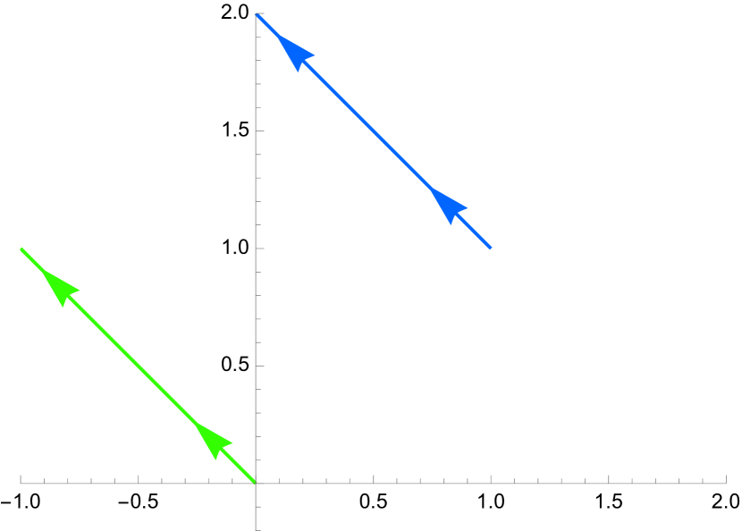
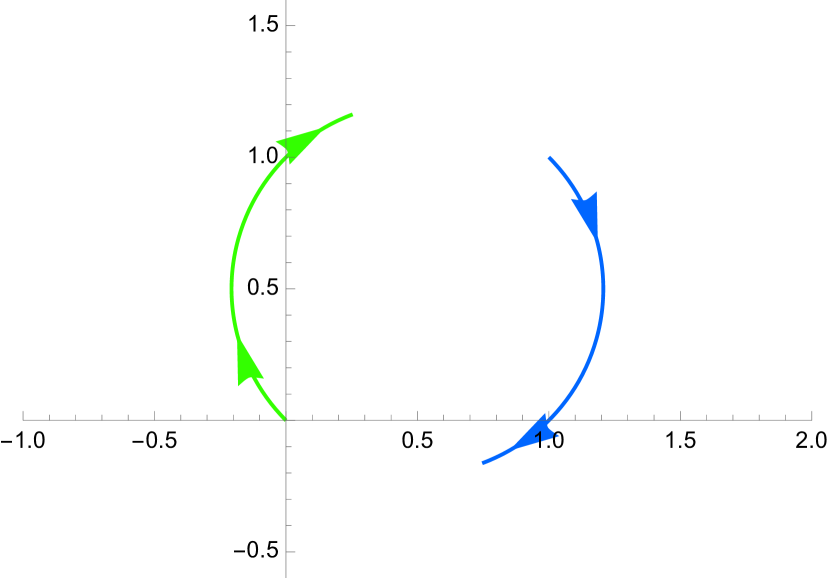
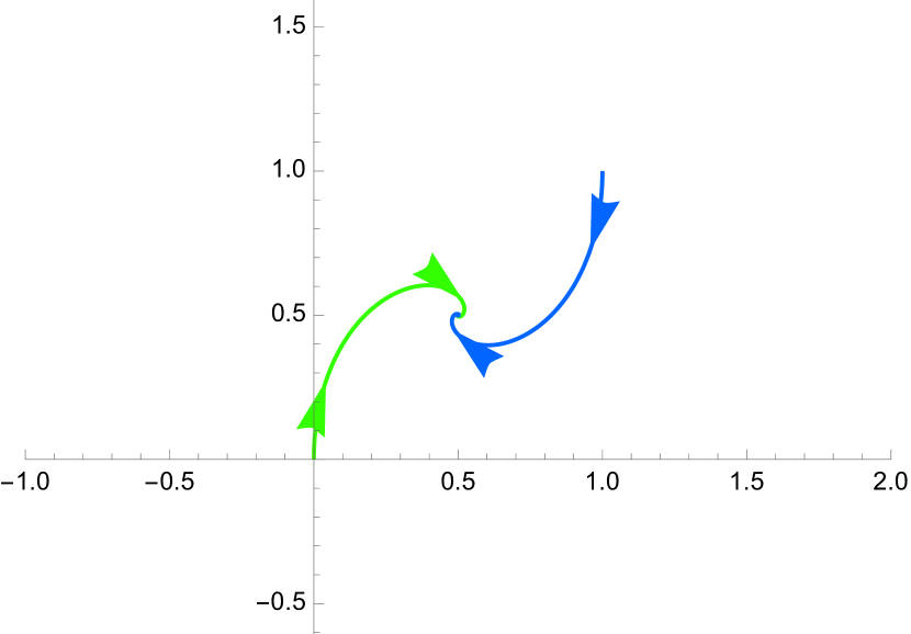
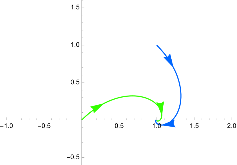
In the formula above, it is clear that both X1subscript𝑋1X_{1} and X2subscript𝑋2X_{2} play specific (but different) roles. We then now give examples of dynamics for a system of N=2𝑁2N=2 particles only. In this case, we can describe the physical meaning of the functional parameters: λisubscript𝜆𝑖\lambda_{i} plays the role of the radial component of the interaction, while μisubscript𝜇𝑖\mu_{i} is the rotational component. In particular:

  • 1.

    λ1>0subscript𝜆10\lambda_{1}>0 promotes convergence, and similarly for λ2<0subscript𝜆20\lambda_{2}<0. Opposite signs promote distancing.

  • 2.

    μ1>0subscript𝜇10\mu_{1}>0 promotes clockwise rotation, and similarly for μ2<0subscript𝜇20\mu_{2}<0. Opposite signs promote counter-clockwise rotation.

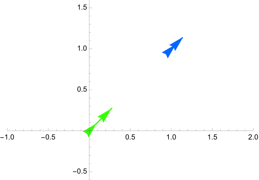
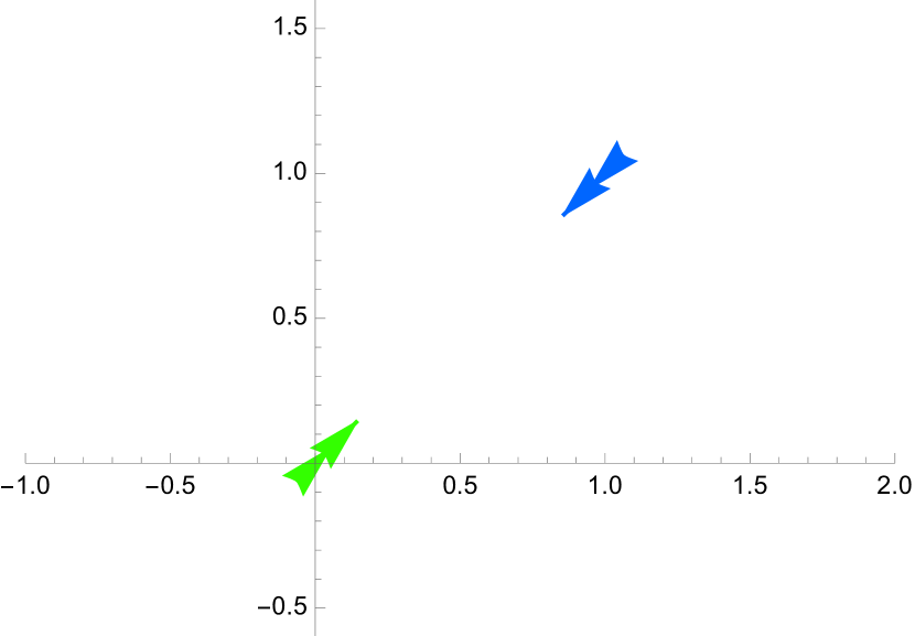
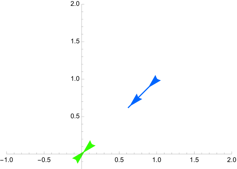
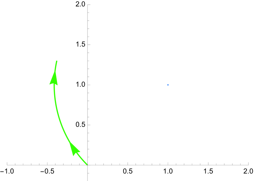
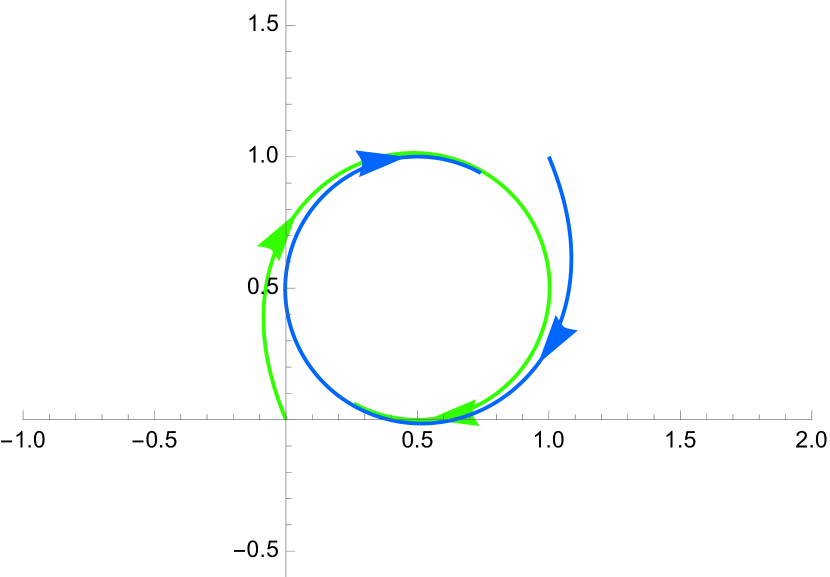
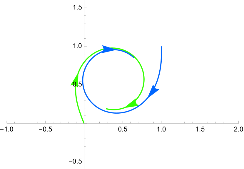
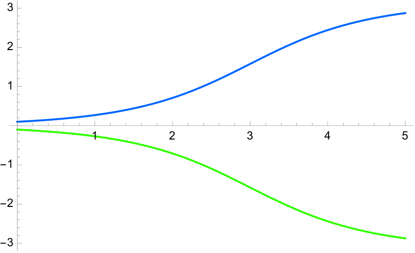
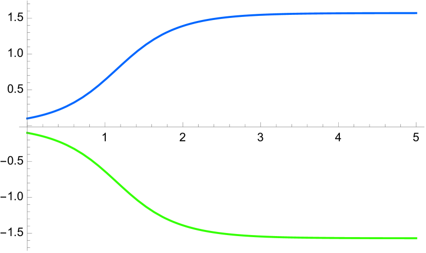
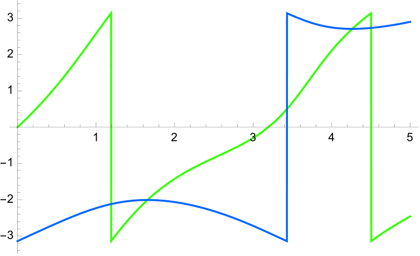
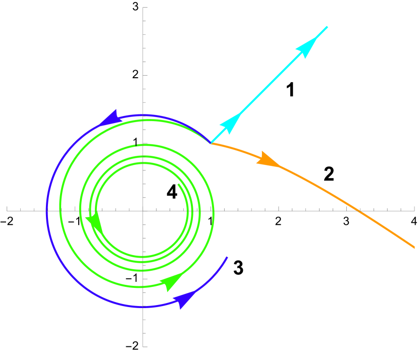
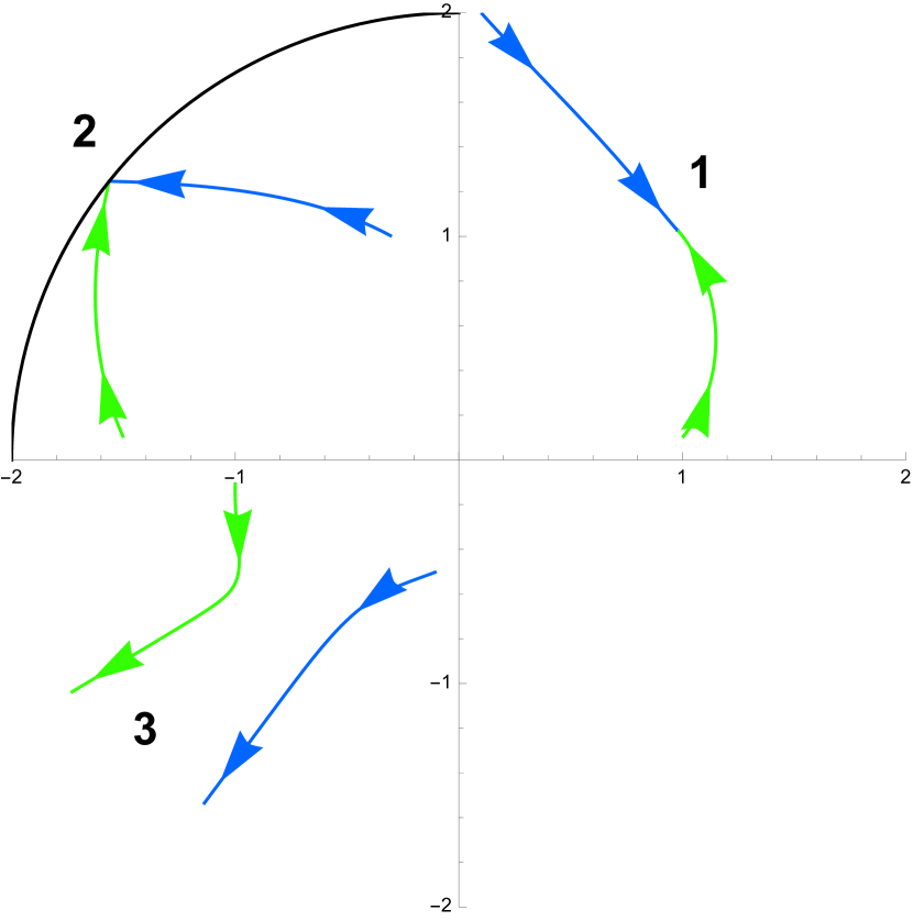
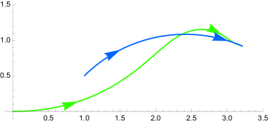
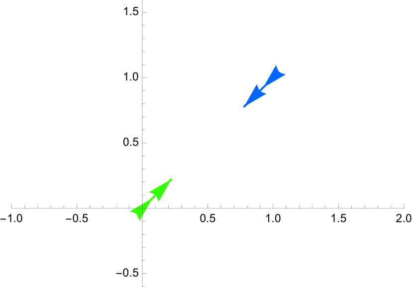
This is made clear from the following examples. Trajectories of these examples can be found in Figure 1. Agent 1 is depicted in green, Agent 2 is depicted in blue. The initial state is always X1=(0,0)subscript𝑋100X_{1}=(0,0), X2=(1,1)subscript𝑋211X_{2}=(1,1).

Example A.1

Set μ1=μ2=0subscript𝜇1subscript𝜇20\mu_{1}=\mu_{2}=0. For λ1=1subscript𝜆11\lambda_{1}=1 and λ2=1subscript𝜆21\lambda_{2}=-1 we have convergence to a common state.

Example A.2

Again with μ1=μ2=0subscript𝜇1subscript𝜇20\mu_{1}=\mu_{2}=0, for λ1=1subscript𝜆11\lambda_{1}=1 and λ2=0.5subscript𝜆20.5\lambda_{2}=0.5, agent 1 aims to converge towards agent 2, that in turn aims to distance itself (with a smaller velocity).

Example A.3

Again with μ1=μ2=0subscript𝜇1subscript𝜇20\mu_{1}=\mu_{2}=0, for λ1=1+ρ2subscript𝜆11subscript𝜌2\lambda_{1}=-1+\rho_{2} and λ2=1ρ2subscript𝜆21subscript𝜌2\lambda_{2}=1-\rho_{2}, agents aim to converge towards a configuration with distance 1.

Example A.4

Again with μ1=μ2=0subscript𝜇1subscript𝜇20\mu_{1}=\mu_{2}=0, for λ1=1+ρ2subscript𝜆11subscript𝜌2\lambda_{1}=-1+\rho_{2} and λ2=0.5ρ2subscript𝜆20.5subscript𝜌2\lambda_{2}=0.5-\rho_{2}, agents aim to converge towards a configuration with different distances (1 and 0,5 respectively). Thus, agent 1 starts converging, then distances itself after reaching distance 1.

Example A.5

Set λ1=λ2=0subscript𝜆1subscript𝜆20\lambda_{1}=\lambda_{2}=0. For μ1=1subscript𝜇11\mu_{1}=1 and μ2=0subscript𝜇20\mu_{2}=0 we have clockwise rotation of agent 1 around agent 2.

Example A.6

Set λ1=λ2=0subscript𝜆1subscript𝜆20\lambda_{1}=\lambda_{2}=0. For μ1=1subscript𝜇11\mu_{1}=1 and μ2=1subscript𝜇21\mu_{2}=1 we have parallel displacement, as agent 1 moves clockwise and agent 2 moves counter-clockwise.

Example A.7

Set λ1=λ2=0subscript𝜆1subscript𝜆20\lambda_{1}=\lambda_{2}=0. For μ1=1subscript𝜇11\mu_{1}=1 and μ2=1subscript𝜇21\mu_{2}=-1 we have clockwise movement.

Example A.8

For λ1=1subscript𝜆11\lambda_{1}=1, λ2=1subscript𝜆21\lambda_{2}=-1, μ1=1subscript𝜇11\mu_{1}=1 and μ2=1subscript𝜇21\mu_{2}=-1 we have clockwise movement, together with convergence.

Example A.9

For λ1=1subscript𝜆11\lambda_{1}=1, λ2=0subscript𝜆20\lambda_{2}=0, μ1=0subscript𝜇10\mu_{1}=0 and μ2=1subscript𝜇21\mu_{2}=1 we have clockwise movement of agent 2 with respect to agent 1, together with convergence of agent 1 towards agent 2 via a radial movement.

Example A.10

For λ1=1+ρ2subscript𝜆11subscript𝜌2\lambda_{1}=-1+\rho_{2} and λ2=1ρ2subscript𝜆21subscript𝜌2\lambda_{2}=1-\rho_{2}, with μ1=1,μ2=1formulae-sequencesubscript𝜇11subscript𝜇21\mu_{1}=1,\mu_{2}=-1 agents aim to converge towards a configuration with distance 1, together with clockwise rotation.

Example A.11

For λ1=1+ρ2subscript𝜆11subscript𝜌2\lambda_{1}=-1+\rho_{2} and λ2=0.5ρ2subscript𝜆20.5subscript𝜌2\lambda_{2}=0.5-\rho_{2}, with μ1=1,μ2=1formulae-sequencesubscript𝜇11subscript𝜇21\mu_{1}=1,\mu_{2}=-1 agents aim to converge towards a configuration with different distances, together with clockwise rotation. The result is a convergence to a limit clockwise trajectory, with distance being the average of the desired distances.

Example A.12

For λ1=0.5+ρ2subscript𝜆10.5subscript𝜌2\lambda_{1}=-0.5+\rho_{2} and λ2=0.5ρ2subscript𝜆20.5subscript𝜌2\lambda_{2}=0.5-\rho_{2}, with μ1=1ρ2,μ2=1+ρ2formulae-sequencesubscript𝜇11subscript𝜌2subscript𝜇21subscript𝜌2\mu_{1}=1-\rho_{2},\mu_{2}=-1+\rho_{2} agents aim to converge towards a configuration with distance 0.5. This first induces counter-clockwise rotation, that then turns into clockwise rotation.
Refer to caption
(a) Example A.1: λ1=1,λ2=1formulae-sequencesubscript𝜆11subscript𝜆21\lambda_{1}=1,\lambda_{2}=-1,
μ1=μ2=0subscript𝜇1subscript𝜇20\mu_{1}=\mu_{2}=0.
Refer to caption
(b) Example A.2: λ1=1,λ2=0.5formulae-sequencesubscript𝜆11subscript𝜆20.5\lambda_{1}=1,\lambda_{2}=0.5,
μ1=μ2=0subscript𝜇1subscript𝜇20\mu_{1}=\mu_{2}=0.
Refer to caption
(c) Ex. A.3: λ1=1+ρ2subscript𝜆11subscript𝜌2\lambda_{1}=-1+\rho_{2},
λ2=1ρ2,μ1=μ2=0formulae-sequencesubscript𝜆21subscript𝜌2subscript𝜇1subscript𝜇20\lambda_{2}=1-\rho_{2},\mu_{1}=\mu_{2}=0.
Refer to caption
(d) Example A.4: λ1=1+ρ2subscript𝜆11subscript𝜌2\lambda_{1}=-1+\rho_{2},
λ2=0.5ρ2,μ1=μ2=0formulae-sequencesubscript𝜆20.5subscript𝜌2subscript𝜇1subscript𝜇20\lambda_{2}=0.5-\rho_{2},\mu_{1}=\mu_{2}=0.
Refer to caption
(e) Example A.5: λ1=λ2=0subscript𝜆1subscript𝜆20\lambda_{1}=\lambda_{2}=0,
μ1=1,μ2=0formulae-sequencesubscript𝜇11subscript𝜇20\mu_{1}=1,\mu_{2}=0.
Refer to caption
(f) Example A.6: λ1=λ2=0subscript𝜆1subscript𝜆20\lambda_{1}=\lambda_{2}=0,
μ1=μ2=1subscript𝜇1subscript𝜇21\mu_{1}=\mu_{2}=1.
Refer to caption
(g) Example A.7: λ1=λ2=0subscript𝜆1subscript𝜆20\lambda_{1}=\lambda_{2}=0,
μ1=1,μ2=1formulae-sequencesubscript𝜇11subscript𝜇21\mu_{1}=1,\mu_{2}=-1.
Refer to caption
(h) Example A.8: λ1=1,λ2=1formulae-sequencesubscript𝜆11subscript𝜆21\lambda_{1}=1,\lambda_{2}=-1,
μ1=1,μ2=1formulae-sequencesubscript𝜇11subscript𝜇21\mu_{1}=1,\mu_{2}=-1.
Refer to caption
(i) Example A.9: λ1=1,λ2=0formulae-sequencesubscript𝜆11subscript𝜆20\lambda_{1}=1,\lambda_{2}=0,
μ1=0,μ2=1formulae-sequencesubscript𝜇10subscript𝜇21\mu_{1}=0,\mu_{2}=1.
Refer to caption
(j) Ex. A.10: λ1=1+ρ2subscript𝜆11subscript𝜌2\lambda_{1}=-1+\rho_{2},
λ2=1ρ2,μ1=1,μ2=1formulae-sequencesubscript𝜆21subscript𝜌2formulae-sequencesubscript𝜇11subscript𝜇21\lambda_{2}=1-\rho_{2},\mu_{1}=1,\mu_{2}=-1.
Refer to caption
(k) Ex. A.11: λ1=1+ρ2subscript𝜆11subscript𝜌2\lambda_{1}=-1+\rho_{2},
λ2=0.5ρ2,μ1=1,μ2=1formulae-sequencesubscript𝜆20.5subscript𝜌2formulae-sequencesubscript𝜇11subscript𝜇21\lambda_{2}=0.5-\rho_{2},\mu_{1}=1,\mu_{2}=-1.
Refer to caption
(l) Ex. A.12: λ1=0.5+ρ2=λ2subscript𝜆10.5subscript𝜌2subscript𝜆2\lambda_{1}=-0.5+\rho_{2}=-\lambda_{2}, μ1=1ρ2=μ2subscript𝜇11subscript𝜌2subscript𝜇2\mu_{1}=1-\rho_{2}=-\mu_{2}.
Figure 1: Examples A (1 to 12).
Remark 30.

The case of M=n𝑀superscript𝑛M=\mathbb{R}^{n} and G=SO(n,)n𝐺left-normal-factor-semidirect-product𝑆𝑂𝑛superscript𝑛G=SO(n,\mathbb{R})\ltimes\mathbb{R}^{n} for n>2𝑛2n>2 is very different. Indeed, in this case, one has =.Idformulae-sequenceId\mathfrak{C}=\mathbb{R}.\mathrm{Id}, hence hypotheses of Corollary 21, Item 1, are never satisfied. Then, one can resort to Corollary 21, Item 2 if N1n𝑁1𝑛N-1\geq n to describe FPD. As it has been already stated in the introduction, our results do not cover “intermediate” number of agents.

Remark 31.

Contrarily to the case described in Remark 30, there is another interesting case in which assumptions of Corollary 21, Item 1 hold: this is the group of unit quaternions \mathcal{H} (or the semi-direct product 4left-normal-factor-semidirect-productsuperscript4\mathcal{H}\ltimes\mathbb{R}^{4}) acting on 4superscript4\mathbb{R}^{4}. Indeed, the Lie algebra \mathcal{L} is generated by the 3 quaternion matrices i,j,k.𝑖𝑗𝑘i,j,k.

i=(0100100000010010),j=(0010000110000100),k=(0001001001001000).formulae-sequence𝑖0100100000010010formulae-sequence𝑗0010000110000100𝑘0001001001001000i=\left(\begin{array}[c]{cccc}0&-1&0&0\\ 1&0&0&0\\ 0&0&0&-1\\ 0&0&1&0\end{array}\right),\qquad j=\left(\begin{array}[c]{cccc}0&0&-1&0\\ 0&0&0&1\\ 1&0&0&0\\ 0&-1&0&0\end{array}\right),\qquad k=\left(\begin{array}[c]{cccc}0&0&0&-1\\ 0&0&-1&0\\ 0&1&0&0\\ 1&0&0&0\end{array}\right).

The centralizer \mathfrak{C} is the full Lie algebra superscript\mathcal{H}^{\ast}of skew quaternions, ={a.Id+b.ı^+c.ȷ^+d.k^}\mathcal{H}^{\ast}=\{a.Id+b.\hat{\imath}+c.\hat{\jmath}+d.\hat{k}\} with

ı^=(0100100000010010),ȷ^=(0010000110000100),k^=(0001001001001000).formulae-sequence^italic-ı0100100000010010formulae-sequence^italic-ȷ0010000110000100^𝑘0001001001001000\hat{\imath}=\left(\begin{array}[c]{cccc}0&-1&0&0\\ 1&0&0&0\\ 0&0&0&1\\ 0&0&-1&0\end{array}\right),\qquad\hat{\jmath}=\left(\begin{array}[c]{cccc}0&0&1&0\\ 0&0&0&1\\ -1&0&0&0\\ 0&-1&0&0\end{array}\right),\qquad\hat{k}=\left(\begin{array}[c]{cccc}0&0&0&-1\\ 0&0&1&0\\ 0&-1&0&0\\ 1&0&0&0\end{array}\right).

It is easy to check that the four vectors x,ı^.x,ȷ^.x,k^.xformulae-sequence𝑥^italic-ı𝑥^italic-ȷ𝑥^𝑘𝑥x,\hat{\imath}.x,\hat{\jmath}.x,\hat{k}.x are independent for all x4{0}𝑥superscript40x\in\mathbb{R}^{4}\setminus\{0\}. Thus, Theorem 2, Item 1 or Corollary 21, Item 1 can be used to characterize the FPD.

3.1 Gradient flows for 2 particles

In the case of N=2𝑁2N=2 particles, we are able to completely characterize the gradient flow PDs.

Proposition 32.

Let F𝐹F be a PD in the FPD associated to (N=2,2,SO(2,)2)𝑁2superscript2left-normal-factor-semidirect-product𝑆𝑂2superscript2(N=2,\mathbb{R}^{2},SO(2,\mathbb{R})\ltimes\mathbb{R}^{2}), i.e. of the form (3.2). Then, it is a gradient flow if and only if λ1=λ2subscript𝜆1subscript𝜆2\lambda_{1}=-\lambda_{2} and μ1=μ2=0subscript𝜇1subscript𝜇20\mu_{1}=\mu_{2}=0.

Proof.

It is easy to prove that both conditions λ1=λ2subscript𝜆1subscript𝜆2\lambda_{1}=-\lambda_{2} and μ1=μ2=0subscript𝜇1subscript𝜇20\mu_{1}=\mu_{2}=0 imply that F𝐹F is a gradient flow. Indeed, define

ϕ(x1,y1,x2,y2):=Φ((x1x2)2+(y1y2)2) with Φ(ρ)=0ρsλ2(s)𝑑sassignitalic-ϕsubscript𝑥1subscript𝑦1subscript𝑥2subscript𝑦2Φsuperscriptsubscript𝑥1subscript𝑥22superscriptsubscript𝑦1subscript𝑦22 with Φ𝜌superscriptsubscript0𝜌𝑠subscript𝜆2𝑠differential-d𝑠\phi(x_{1},y_{1},x_{2},y_{2}):=\Phi(\sqrt{(x_{1}-x_{2})^{2}+(y_{1}-y_{2})^{2}})\mbox{~{}~{}with~{}~{}}\Phi(\rho)=\int_{0}^{\rho}\sqrt{s}\lambda_{2}(s)\,ds

and check that F=ϕ𝐹italic-ϕF=\nabla\phi.

We now prove the converse result. Let ϕ(x1,x2,x2,y2)italic-ϕsubscript𝑥1subscript𝑥2subscript𝑥2subscript𝑦2\phi(x_{1},x_{2},x_{2},y_{2}) be such that ϕitalic-ϕ\nabla\phi is a PD, i.e. of the form (3.2). A direct computation shows that, by imposing that f1,1=x1ϕsubscript𝑓11subscriptsubscript𝑥1italic-ϕf_{1,1}=\partial_{x_{1}}\phi and f2,1=x2ϕsubscript𝑓21subscriptsubscript𝑥2italic-ϕf_{2,1}=\partial_{x_{2}}\phi, the condition x2f1,1=x1f2,1subscriptsubscript𝑥2subscript𝑓11subscriptsubscript𝑥1subscript𝑓21\partial_{x_{2}}f_{1,1}=\partial_{x_{1}}f_{2,1} ensures λ1=λ2subscript𝜆1subscript𝜆2\lambda_{1}=-\lambda_{2} and μ1=μ2subscript𝜇1subscript𝜇2\mu_{1}=-\mu_{2}. We already know that the dynamics given by λ1=λ2subscript𝜆1subscript𝜆2\lambda_{1}=-\lambda_{2} with μ1=μ2=0subscript𝜇1subscript𝜇20\mu_{1}=\mu_{2}=0 is a gradient flow, as proved above. By recalling that gradient flows form a vector space, we can then focus on the case λ1=λ2=0subscript𝜆1subscript𝜆20\lambda_{1}=\lambda_{2}=0 and μ1=μ2subscript𝜇1subscript𝜇2\mu_{1}=-\mu_{2}.

We now impose the condition y2f2,1=x2f2,2subscriptsubscript𝑦2subscript𝑓21subscriptsubscript𝑥2subscript𝑓22\partial_{y_{2}}f_{2,1}=\partial_{x_{2}}f_{2,2}, that reads as

μ2(ρ2)+(y1y2)ρ2μ2(ρ2)y2y1ρ2=μ2(ρ2)+(x2x1)ρ2μ2(ρ2)x2x1ρ2,subscript𝜇2subscript𝜌2subscript𝑦1subscript𝑦2subscriptsubscript𝜌2subscript𝜇2subscript𝜌2subscript𝑦2subscript𝑦1subscript𝜌2subscript𝜇2subscript𝜌2subscript𝑥2subscript𝑥1subscriptsubscript𝜌2subscript𝜇2subscript𝜌2subscript𝑥2subscript𝑥1subscript𝜌2\displaystyle-\mu_{2}(\rho_{2})+(y_{1}-y_{2})\partial_{\rho_{2}}\mu_{2}(\rho_{2})\frac{y_{2}-y_{1}}{\rho_{2}}=\mu_{2}(\rho_{2})+(x_{2}-x_{1})\partial_{\rho_{2}}\mu_{2}(\rho_{2})\frac{x_{2}-x_{1}}{\rho_{2}},

hence 2μ2(ρ2)+ρ2ρ2μ2(ρ2)=02subscript𝜇2subscript𝜌2subscript𝜌2subscriptsubscript𝜌2subscript𝜇2subscript𝜌202\mu_{2}(\rho_{2})+\rho_{2}\partial_{\rho_{2}}\mu_{2}(\rho_{2})=0. This implies μ2(ρ2)=kρ22subscript𝜇2subscript𝜌2𝑘superscriptsubscript𝜌22\mu_{2}(\rho_{2})=\frac{k}{\rho_{2}^{2}}. Remark that the domain is clearly given by ρ20subscript𝜌20\rho_{2}\neq 0, that is a G𝐺G-invariant set. Again by recalling that gradient flows form a vector space, we see that we need only to check wether the following vector field is a gradient flow:

x˙1=y2y1ρ22,y˙1=x1x2ρ22,x˙2=y1y2ρ22,y˙2=x2x1ρ22.formulae-sequencesubscript˙𝑥1subscript𝑦2subscript𝑦1superscriptsubscript𝜌22formulae-sequencesubscript˙𝑦1subscript𝑥1subscript𝑥2superscriptsubscript𝜌22formulae-sequencesubscript˙𝑥2subscript𝑦1subscript𝑦2superscriptsubscript𝜌22subscript˙𝑦2subscript𝑥2subscript𝑥1superscriptsubscript𝜌22\dot{x}_{1}=\frac{y_{2}-y_{1}}{\rho_{2}^{2}},\qquad\dot{y}_{1}=\frac{x_{1}-x_{2}}{\rho_{2}^{2}},\qquad\dot{x}_{2}=\frac{y_{1}-y_{2}}{\rho_{2}^{2}},\qquad\dot{y}_{2}=\frac{x_{2}-x_{1}}{\rho_{2}^{2}}. (3.3)

By duality in 4superscript4\mathbb{R}^{4}, it is a gradient flow if and only if the dual 1-form

ω=(y1y2)d(x2x1)+(x2x1)d(y2y1)ρ22𝜔subscript𝑦1subscript𝑦2𝑑subscript𝑥2subscript𝑥1subscript𝑥2subscript𝑥1𝑑subscript𝑦2subscript𝑦1superscriptsubscript𝜌22\omega=\frac{(y_{1}-y_{2})d(x_{2}-x_{1})+(x_{2}-x_{1})d(y_{2}-y_{1})}{\rho_{2}^{2}}

is exact. By writing it in coordinates (ρ2,θ2,x2,y2)subscript𝜌2subscript𝜃2subscript𝑥2subscript𝑦2(\rho_{2},\theta_{2},x_{2},y_{2}) with ρ2(cos(θ2),sin(θ2))=(x2x1,y2y1)subscript𝜌2subscript𝜃2subscript𝜃2subscript𝑥2subscript𝑥1subscript𝑦2subscript𝑦1\rho_{2}(\cos(\theta_{2}),\sin(\theta_{2}))=(x_{2}-x_{1},y_{2}-y_{1}), we have ω=dθ2𝜔𝑑subscript𝜃2\omega=d\theta_{2}. It is clear that this form is not exact. Thus, the vector field (3.3) is not a gradient flow. This in turn implies that a gradient flow that is a PD necessarily satisfies μ1=μ2=0subscript𝜇1subscript𝜇20\mu_{1}=\mu_{2}=0. ∎

Remark 33.

The proof above shows that a complete characterization of gradient flow PDs is difficult, since one needs to check wether forms are exact on domains that are not simply connected. For this reason, we have no complete characterization for the case N>2𝑁2N>2, for which we only have the partial results given by Proposition 24.

3.2 Permutation-equivariant population dynamics

We now add permutation equivariance to the previous setting, by studying FPEPD introduced in Definition 10. Since we already observed that the centralizer \mathfrak{C} of SO(2,)𝑆𝑂2SO(2,\mathbb{R}) has dimension n=2𝑛2n=2, we can apply Corollary 22 to compute the FPEPD in this case. We have the following result.

Proposition 34.

Consider the FPEPD associated to (N,2,SO(2,)2)𝑁superscript2left-normal-factor-semidirect-product𝑆𝑂2superscript2(N,\mathbb{R}^{2},SO(2,\mathbb{R})\ltimes\mathbb{R}^{2}) with N>1𝑁1N>1.

Consider the dynamics taking place on the open dense set

𝒪𝒪\displaystyle\mathcal{O} =\displaystyle= {(X1,,XN)2N such that ji(XjXi)(0,0) for all i=1,,N}.formulae-sequencesubscript𝑋1subscript𝑋𝑁superscript2𝑁 such that subscript𝑗𝑖subscript𝑋𝑗subscript𝑋𝑖00 for all 𝑖1𝑁\displaystyle\Big{\{}(X_{1},\ldots,X_{N})\in\mathbb{R}^{2N}\mbox{~{}~{}such that~{}~{}}\sum_{j\neq i}(X_{j}-X_{i})\neq(0,0)\mbox{~{}for all~{}}i=1,\ldots,N\Big{\}}.

Write in polar coordinates XjXi=ρj,i(cos(θj,i),sin(θj,i))subscript𝑋𝑗subscript𝑋𝑖subscript𝜌𝑗𝑖subscript𝜃𝑗𝑖subscript𝜃𝑗𝑖X_{j}-X_{i}=\rho_{j,i}(\cos(\theta_{j,i}),\sin(\theta_{j,i})) and define τj,i:=θj,iθi+1,iassignsubscript𝜏𝑗𝑖subscript𝜃𝑗𝑖subscript𝜃𝑖1𝑖\tau_{j,i}:=\theta_{j,i}-\theta_{i+1,i}, with the convention that i=N+1𝑖𝑁1i=N+1 is replaced by i=1𝑖1i=1 and that the difference of angles is mod-2π2𝜋2\pi.

Then, the FPEPD is composed of all vector fields of the form

F=F1++FN with Fi=fi,1xi+fi,2yi,formulae-sequence𝐹subscript𝐹1subscript𝐹𝑁 with subscript𝐹𝑖subscript𝑓𝑖1subscriptsubscript𝑥𝑖subscript𝑓𝑖2subscriptsubscript𝑦𝑖F=F_{1}+\ldots+F_{N}\qquad\mbox{~{}~{}with~{}~{}}\qquad F_{i}=f_{i,1}\partial_{x_{i}}+f_{i,2}\partial_{y_{i}},

and

(fi,1fi,2)=(ji(xjxi)ji(yjyi)ji(yjyi)ji(xjxi))(λ(ρˇi,τiˇ)μ(ρˇi,τiˇ)),subscript𝑓𝑖1subscript𝑓𝑖2subscript𝑗𝑖subscript𝑥𝑗subscript𝑥𝑖subscript𝑗𝑖subscript𝑦𝑗subscript𝑦𝑖subscript𝑗𝑖subscript𝑦𝑗subscript𝑦𝑖subscript𝑗𝑖subscript𝑥𝑗subscript𝑥𝑖binomial𝜆subscriptˇ𝜌𝑖ˇsubscript𝜏𝑖𝜇subscriptˇ𝜌𝑖ˇsubscript𝜏𝑖\left(\begin{array}[c]{c}f_{i,1}\\ f_{i,2}\end{array}\right)=\left(\begin{array}[c]{cc}\sum_{j\neq i}(x_{j}-x_{i})&-\sum_{j\neq i}(y_{j}-y_{i})\\ \sum_{j\neq i}(y_{j}-y_{i})&\sum_{j\neq i}(x_{j}-x_{i})\end{array}\right)\binom{\lambda(\check{\rho}_{i},\check{\tau_{i}})}{\mu(\check{\rho}_{i},\check{\tau_{i}})},

where functions λ,μ𝜆𝜇\lambda,\mu are arbitrary analytic functions that are invariant with respect to permutations of both the first N1𝑁1N-1 coordinates

ρˇi:=(ρ1,i,,ρi1,i,ρi+1,i,,ρN,i)assignsubscriptˇ𝜌𝑖subscript𝜌1𝑖subscript𝜌𝑖1𝑖subscript𝜌𝑖1𝑖subscript𝜌𝑁𝑖\check{\rho}_{i}:=(\rho_{1,i},\ldots,\rho_{i-1,i},\rho_{i+1,i},\ldots,\rho_{N,i})

and the remaining N2𝑁2N-2 coordinates

τˇi:=(τ1,i,,τi1,i,τi+2,i,,τN,i).assignsubscriptˇ𝜏𝑖subscript𝜏1𝑖subscript𝜏𝑖1𝑖subscript𝜏𝑖2𝑖subscript𝜏𝑁𝑖\check{\tau}_{i}:=(\tau_{1,i},\ldots,\tau_{i-1,i},\tau_{i+2,i},\ldots,\tau_{N,i}).
Proof.

The proof is a direct application of Corollary 22. The only remarkable detail is that all functions that are jointly radial (i.e. invariant by rototranslation) and permutation invariant are of the form λ,μ𝜆𝜇\lambda,\mu given in the statement; this fact has already been proved for Proposition 28. ∎

Remark 35.

This result, combined with Proposition 32, shows that the only possible PDs for N=2𝑁2N=2 that are gradient flows are also PEPDs.

We do not provide additional examples. For N=2𝑁2N=2 particles, we already had PEPD in Examples A.(1-3-7-8-10-12) in Figure 1. Examples for N>2𝑁2N>2 particles are similar, again with λ>0𝜆0\lambda>0 promoting convergence and μ>0𝜇0\mu>0 promoting clockwise rotation.

4 Population Dynamics on the relativistic spaces

In this section, we focus on Population Dynamics on the relativistic spaces.

4.1 Population Dynamics on the relativistic line

In this section, we deal with PDs on the relativistic line: the state space is the pseudo-Euclidean plane 2superscript2\mathbb{R}^{2} endowed with the quadratic form with signature (1,1)11(1,1). We denote by c>0𝑐0c>0 the speed of light and consider the following scalar product:

(T1,x1)(T2,x2)=c2T1T2x1x2.subscript𝑇1subscript𝑥1subscript𝑇2subscript𝑥2superscript𝑐2subscript𝑇1subscript𝑇2subscript𝑥1subscript𝑥2(T_{1},x_{1})\cdot(T_{2},x_{2})=c^{2}T_{1}T_{2}-x_{1}x_{2}.

The group is the semidirect product G=SO(1,1)2𝐺left-normal-factor-semidirect-product𝑆𝑂11superscript2G=SO(1,1)\ltimes\mathbb{R}^{2} that preserves the associated quadratic form. We have the following result.

Proposition 36.

Consider the FPD associated to (N,2,SO(1,1)2)𝑁superscript2left-normal-factor-semidirect-product𝑆𝑂11superscript2(N,\mathbb{R}^{2},SO(1,1)\ltimes\mathbb{R}^{2}). Then:

  • 1.

    for N=1𝑁1N=1, the FPD contains the zero vector field only;

  • 2.

    for N=2𝑁2N=2, all PDs are given by F=F1+F2𝐹subscript𝐹1subscript𝐹2F=F_{1}+F_{2} with Fi=fi,1Ti+fi,2xisubscript𝐹𝑖subscript𝑓𝑖1subscriptsubscript𝑇𝑖subscript𝑓𝑖2subscriptsubscript𝑥𝑖F_{i}=f_{i,1}\partial_{T_{i}}+f_{i,2}\partial_{x_{i}}, where

    (fi,1fi,2)=(T2T1c1(x2x1)x2x1c(T2T1))(ϕi(r)ψi(r))subscript𝑓𝑖1subscript𝑓𝑖2subscript𝑇2subscript𝑇1superscript𝑐1subscript𝑥2subscript𝑥1subscript𝑥2subscript𝑥1𝑐subscript𝑇2subscript𝑇1subscriptitalic-ϕ𝑖𝑟subscript𝜓𝑖𝑟\left(\begin{array}[c]{c}f_{i,1}\\ f_{i,2}\end{array}\right)=\left(\begin{array}[c]{cc}T_{2}-T_{1}&c^{-1}(x_{2}-x_{1})\\ x_{2}-x_{1}&c(T_{2}-T_{1})\end{array}\right)\left(\begin{array}[]{c}\phi_{i}(r)\\ \psi_{i}(r)\end{array}\right)

    with ϕi(r),ψi(r)subscriptitalic-ϕ𝑖𝑟subscript𝜓𝑖𝑟\phi_{i}(r),\psi_{i}(r) analytic functions of r=c2(T2T1)2(x2x1)2𝑟superscript𝑐2superscriptsubscript𝑇2subscript𝑇12superscriptsubscript𝑥2subscript𝑥12r=\sqrt{c^{2}(T_{2}-T_{1})^{2}-(x_{2}-x_{1})^{2}};

  • 3.

    for N3𝑁3N\geq 3, and choosing any two distinct indexes k1,k2{2,,N}subscript𝑘1subscript𝑘22𝑁k_{1},k_{2}\in\{2,\ldots,N\}, all PDs are of the form

    F(X)=i=1Nfi(Z)Xi with fi=ψi,1(Z)Zk1+ψi,2(Z)Zk2,formulae-sequence𝐹𝑋superscriptsubscript𝑖1𝑁subscript𝑓𝑖𝑍subscriptsubscript𝑋𝑖 with subscript𝑓𝑖subscript𝜓𝑖1𝑍subscript𝑍subscript𝑘1subscript𝜓𝑖2𝑍subscript𝑍subscript𝑘2F(X)=\sum_{i=1}^{N}f_{i}(Z)\partial_{X_{i}}\qquad\mbox{~{}~{} with ~{}~{}}\qquad f_{i}=\psi_{i,1}(Z)Z_{k_{1}}+\psi_{i,2}(Z)Z_{k_{2}},

    where ψi,k(Z)subscript𝜓𝑖𝑘𝑍\psi_{i,k}(Z) are 𝔏^^𝔏\hat{\mathfrak{L}}-jointly radial functions of Z=(Z2,,ZN)𝑍subscript𝑍2subscript𝑍𝑁Z=(Z_{2},\ldots,Z_{N}) with Zi:=(TiT1,xix1)assignsubscript𝑍𝑖subscript𝑇𝑖subscript𝑇1subscript𝑥𝑖subscript𝑥1Z_{i}:=(T_{i}-T_{1},x_{i}-x_{1}).

Proof.

For N=1𝑁1N=1, we have that Proposition 19 ensures that PDs are contained in the set of constant vector fields. By adding equivariance with respect to SO(1,1)𝑆𝑂11SO(1,1), we have that the only PD is the zero vector field.

The case N3𝑁3N\geq 3 is a direct application of Corollary 21, Item 2. One can also apply Corollary 21, Item 1.

The case N=2𝑁2N=2 is a direct application of Corollary 21, Item 1. Indeed, the centralizer of so(1,1)=.Kformulae-sequence𝑠𝑜11𝐾so(1,1)=\mathbb{R}.K with

K=(0c1c0)𝐾0superscript𝑐1𝑐0K=\left(\begin{array}[]{cc}0&c^{-1}\\ c&0\end{array}\right)

is =.Id+.Kformulae-sequenceId𝐾\mathfrak{C}=\mathbb{R}.\mathrm{Id}+\mathbb{R}.K, that has dimension n=2𝑛2n=2. Then, solutions are of the form ϕ(Z)Z+ψ(Z)KZitalic-ϕ𝑍𝑍𝜓𝑍𝐾𝑍\phi(Z)Z+\psi(Z)KZ, where Z=(T2T1,x2x1)𝑍subscript𝑇2subscript𝑇1subscript𝑥2subscript𝑥1Z=(T_{2}-T_{1},x_{2}-x_{1}). Moreover, ϕ(Z),ψ(Z)italic-ϕ𝑍𝜓𝑍\phi(Z),\psi(Z) are so(1,1)𝑠𝑜11so(1,1)-radial, thus depending on r=Z=c2(T2T1)2(x2x1)2𝑟norm𝑍superscript𝑐2superscriptsubscript𝑇2subscript𝑇12superscriptsubscript𝑥2subscript𝑥12r=\|Z\|=\sqrt{c^{2}(T_{2}-T_{1})^{2}-(x_{2}-x_{1})^{2}} only.

Remark 37.

The case N=2𝑁2N=2 is an interesting example in which it holds SSSS\mathcal{E}\subsetneq\SS, i.e. in which elementary solutions do not provide all solutions. We can anyway provide a complete classification, due to the equality 𝒞=SS𝒞SS\mathcal{C}=\SS, i.e. observing that all solutions are solutions given by the centralizer.

Remark 38.

A direct computation for N=2𝑁2N=2 shows that r˙=r(ϕ1(r)ϕ2(r))˙𝑟𝑟subscriptitalic-ϕ1𝑟subscriptitalic-ϕ2𝑟\dot{r}=r(\phi_{1}(r)-\phi_{2}(r)). In particular, this implies that terms ψ1,ψ2subscript𝜓1subscript𝜓2\psi_{1},\psi_{2} do not contribute to the dynamics of r𝑟r (i.e. the dynamics on the quotient space).

We now provide some simple examples for N=2𝑁2N=2. In Examples B.1-2-3, we consider the case of ϕ1(r)=rsubscriptitalic-ϕ1𝑟𝑟\phi_{1}(r)=r, ϕ2(r)=1subscriptitalic-ϕ2𝑟1\phi_{2}(r)=1 and ψ1=ψ2=0subscript𝜓1subscript𝜓20\psi_{1}=\psi_{2}=0 with increasing values of c{1,10,100}𝑐110100c\in\{1,10,100\}. By Remark 38, it holds tr(t)=r(1r)subscript𝑡𝑟𝑡𝑟1𝑟\partial_{t}r(t)=r(1-r), hence the variable r𝑟r converges to the value 1. The limit dynamics is then given by ϕ1=ϕ2=1subscriptitalic-ϕ1subscriptitalic-ϕ21\phi_{1}=\phi_{2}=1, i.e. translations with constant velocity 1 in all variables T1,x1,T2,x2subscript𝑇1subscript𝑥1subscript𝑇2subscript𝑥2T_{1},x_{1},T_{2},x_{2}. This corresponds to the fact that the relativistic dynamics converges to the so-called relative equilibria of the classical dynamics, i.e. classical dynamics with constant x1x2subscript𝑥1subscript𝑥2x_{1}-x_{2}. The key remark here is that the convergence of the relativistic dynamics to the classical one is faster when values of c𝑐c increase, as expected.

In Examples B.4-5-6, we investigate the role of ψ1,ψ2subscript𝜓1subscript𝜓2\psi_{1},\psi_{2}. They do not contribute to the dynamics of the variable r𝑟r, but we show that they play a strong role in the dynamics of the state variable. In particular, we show that the dynamics is qualitatively different for different values of the parameter c{1,10,100}𝑐110100c\in\{1,10,100\}. We choose again ϕ1(r)=rsubscriptitalic-ϕ1𝑟𝑟\phi_{1}(r)=r, ϕ2(r)=1subscriptitalic-ϕ2𝑟1\phi_{2}(r)=1, ensuring convergence of r𝑟r to 1. By defining ψ1=100/c=ψ2subscript𝜓1100𝑐subscript𝜓2\psi_{1}=100/c=-\psi_{2}, we find that:

  • 1.

    for c=1𝑐1c=1 the distances T2T1,x2x1subscript𝑇2subscript𝑇1subscript𝑥2subscript𝑥1T_{2}-T_{1},x_{2}-x_{1} explode;

  • 2.

    for c=10𝑐10c=10 the distance T2T1subscript𝑇2subscript𝑇1T_{2}-T_{1} converges to 0, while x2x1subscript𝑥2subscript𝑥1x_{2}-x_{1} converges to a constant (i.e. to a classical relative equilibrium);

  • 3.

    for c=100𝑐100c=100 the dynamics is similar to the case c=10𝑐10c=10, but convergence is faster for both variables.
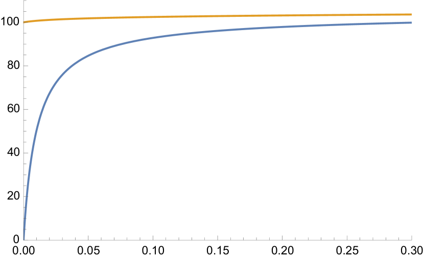
Refer to caption
Refer to caption
Refer to caption
Refer to caption
(a) Example B.1 with c=1𝑐1c=1.
Refer to caption
(b) Example B.2 with c=10𝑐10c=10.
Refer to caption
(c) Example B.3 with c=100𝑐100c=100.
Refer to caption
Refer to caption
Refer to caption
Refer to caption
(d) Example B.4 with c=1𝑐1c=1.
Refer to caption
(e) Example B.5 with c=10𝑐10c=10.
Refer to caption
(f) Example B.6 with c=100𝑐100c=100.
Figure 2: Examples B (1 to 6). Variables T𝑇T above, x𝑥x below; Variables 1 (blue) and 2 (orange).

4.2 Population Dynamics on the relativistic plane

In this section, we deal with PDs on the relativistic plane: the state space is the pseudo-Euclidean space 3superscript3\mathbb{R}^{3} endowed with the quadratic form with signature (1,2)12(1,2). Given two states (T1,x1,y1)subscript𝑇1subscript𝑥1subscript𝑦1(T_{1},x_{1},y_{1}), (T2,x2,y2)subscript𝑇2subscript𝑥2subscript𝑦2(T_{2},x_{2},y_{2}), the scalar product is

(T1,x1,y1)(T2,x2,y2)=T1T2x1x2y1y2.subscript𝑇1subscript𝑥1subscript𝑦1subscript𝑇2subscript𝑥2subscript𝑦2subscript𝑇1subscript𝑇2subscript𝑥1subscript𝑥2subscript𝑦1subscript𝑦2(T_{1},x_{1},y_{1})\cdot(T_{2},x_{2},y_{2})=T_{1}T_{2}-x_{1}x_{2}-y_{1}y_{2}.

The group is then the semidirect product G=SO(1,2)3𝐺left-normal-factor-semidirect-product𝑆𝑂12superscript3G=SO(1,2)\ltimes\mathbb{R}^{3}. We treat the cases N=1𝑁1N=1 and N4𝑁4N\geq 4 with the general theory. We are then left with two special dimensions, that are N=2,3𝑁23N=2,3. For N=2𝑁2N=2, we prove that PDs are determined by elementary solutions via a direct computation. Instead, for N=3𝑁3N=3 we have no general statement. The results are summarized as follows.

Proposition 39.

Consider the FPD associated to (N,3,SO(1,2)3)𝑁superscript3left-normal-factor-semidirect-product𝑆𝑂12superscript3(N,\mathbb{R}^{3},SO(1,2)\ltimes\mathbb{R}^{3}). Then:

  • 1.

    for N=1𝑁1N=1, the FPD is composed of the zero vector field only;

  • 2.

    for N=2𝑁2N=2, all PDs are of the form

    F(X1,X2)𝐹subscript𝑋1subscript𝑋2\displaystyle F(X_{1},X_{2}) =\displaystyle= ψ1(r)((T2T1)T1+(x2x1)x1+(y2y1)y1)+limit-fromsubscript𝜓1𝑟subscript𝑇2subscript𝑇1subscriptsubscript𝑇1subscript𝑥2subscript𝑥1subscriptsubscript𝑥1subscript𝑦2subscript𝑦1subscriptsubscript𝑦1\displaystyle\psi_{1}(r)\left((T_{2}-T_{1})\partial_{T_{1}}+(x_{2}-x_{1})\partial_{x_{1}}+(y_{2}-y_{1})\partial_{y_{1}}\right)+
    ψ2(r)((T2T1)T2+(x2x1)x2+(y2y1)y2),subscript𝜓2𝑟subscript𝑇2subscript𝑇1subscriptsubscript𝑇2subscript𝑥2subscript𝑥1subscriptsubscript𝑥2subscript𝑦2subscript𝑦1subscriptsubscript𝑦2\displaystyle\psi_{2}(r)\left((T_{2}-T_{1})\partial_{T_{2}}+(x_{2}-x_{1})\partial_{x_{2}}+(y_{2}-y_{1})\partial_{y_{2}}\right),

    with r=(T2T1)2(x2x1)2(y2y1)2𝑟superscriptsubscript𝑇2subscript𝑇12superscriptsubscript𝑥2subscript𝑥12superscriptsubscript𝑦2subscript𝑦12r=\sqrt{(T_{2}-T_{1})^{2}-(x_{2}-x_{1})^{2}-(y_{2}-y_{1})^{2}};

  • 3.

    for N=3𝑁3N=3, the FPD contains vector fields of the form

    F(X1,X2,X3)𝐹subscript𝑋1subscript𝑋2subscript𝑋3\displaystyle F(X_{1},X_{2},X_{3}) =\displaystyle= i=13ϕi(Z2,Z3)((T2T1)Ti+(x2x1)xi+(y2y1)yi)+limit-fromsuperscriptsubscript𝑖13subscriptitalic-ϕ𝑖subscript𝑍2subscript𝑍3subscript𝑇2subscript𝑇1subscriptsubscript𝑇𝑖subscript𝑥2subscript𝑥1subscriptsubscript𝑥𝑖subscript𝑦2subscript𝑦1subscriptsubscript𝑦𝑖\displaystyle\sum_{i=1}^{3}\phi_{i}(Z_{2},Z_{3})\left((T_{2}-T_{1})\partial_{T_{i}}+(x_{2}-x_{1})\partial_{x_{i}}+(y_{2}-y_{1})\partial_{y_{i}}\right)+
    ψi(Z2,Z3)((T3T1)Ti+(x3x1)xi+(y3y1)yi),subscript𝜓𝑖subscript𝑍2subscript𝑍3subscript𝑇3subscript𝑇1subscriptsubscript𝑇𝑖subscript𝑥3subscript𝑥1subscriptsubscript𝑥𝑖subscript𝑦3subscript𝑦1subscriptsubscript𝑦𝑖\displaystyle\psi_{i}(Z_{2},Z_{3})\left((T_{3}-T_{1})\partial_{T_{i}}+(x_{3}-x_{1})\partial_{x_{i}}+(y_{3}-y_{1})\partial_{y_{i}}\right),

    with

    Z2:=(T2T1,x2x1,y2y1),Z3:=(T3T1,x3x1,y3y1)formulae-sequenceassignsubscript𝑍2subscript𝑇2subscript𝑇1subscript𝑥2subscript𝑥1subscript𝑦2subscript𝑦1assignsubscript𝑍3subscript𝑇3subscript𝑇1subscript𝑥3subscript𝑥1subscript𝑦3subscript𝑦1Z_{2}:=(T_{2}-T_{1},x_{2}-x_{1},y_{2}-y_{1}),\qquad Z_{3}:=(T_{3}-T_{1},x_{3}-x_{1},y_{3}-y_{1})

    and ϕi,ψisubscriptitalic-ϕ𝑖subscript𝜓𝑖\phi_{i},\psi_{i} analytic and 𝔏^^𝔏\hat{\mathfrak{L}}-jointly radial with respect to the action of SO(1,2)𝑆𝑂12SO(1,2);

  • 4.

    for N4𝑁4N\geq 4, and choosing any three distinct indexes k1,k2,k3{1,,N}subscript𝑘1subscript𝑘2subscript𝑘31𝑁k_{1},k_{2},k_{3}\in\{1,\ldots,N\}, all PDs are of the form

    F(X)=i=1Nfi(Z)Xi with fi=ψi,1(Z)Zk1+ψi,2(Z)Zk2+ψi,3(Z)Zk3,formulae-sequence𝐹𝑋superscriptsubscript𝑖1𝑁subscript𝑓𝑖𝑍subscriptsubscript𝑋𝑖 with subscript𝑓𝑖subscript𝜓𝑖1𝑍subscript𝑍subscript𝑘1subscript𝜓𝑖2𝑍subscript𝑍subscript𝑘2subscript𝜓𝑖3𝑍subscript𝑍subscript𝑘3F(X)=\sum_{i=1}^{N}f_{i}(Z)\partial_{X_{i}}\qquad\mbox{~{}~{} with ~{}~{}}\qquad f_{i}=\psi_{i,1}(Z)Z_{k_{1}}+\psi_{i,2}(Z)Z_{k_{2}}+\psi_{i,3}(Z)Z_{k_{3}},

    where ψi,k(Z)subscript𝜓𝑖𝑘𝑍\psi_{i,k}(Z) are 𝔏^^𝔏\hat{\mathfrak{L}}-jointly radial functions of Z=(Z2,,ZN)𝑍subscript𝑍2subscript𝑍𝑁Z=(Z_{2},\ldots,Z_{N}) with Zi:=(TiT1,xix1,yiy1)assignsubscript𝑍𝑖subscript𝑇𝑖subscript𝑇1subscript𝑥𝑖subscript𝑥1subscript𝑦𝑖subscript𝑦1Z_{i}:=(T_{i}-T_{1},x_{i}-x_{1},y_{i}-y_{1}).

Proof.

The cases N=1𝑁1N=1 and N4𝑁4N\geq 4 are identical to Proposition 36.

We now study N=2𝑁2N=2, for which we introduce the difference variable

Z=(T,x,y):=(T2T1,x2x1,y2y1)𝑍𝑇𝑥𝑦assignsubscript𝑇2subscript𝑇1subscript𝑥2subscript𝑥1subscript𝑦2subscript𝑦1Z=(T,x,y):=(T_{2}-T_{1},x_{2}-x_{1},y_{2}-y_{1})

and consider vector fields of a single particle of coordinate Z𝑍Z that are equivariant under the action of SO(1,2)𝑆𝑂12SO(1,2), i.e. solutions of (2.13). For this reason, we introduce polar coordinates in the (x,y)𝑥𝑦(x,y) difference variables, i.e.

(x2x1,y2y1)=ρ(cos(θ),sin(θ)) with ρ0,θ[0,2π).formulae-sequencesubscript𝑥2subscript𝑥1subscript𝑦2subscript𝑦1𝜌𝜃𝜃 with 𝜌0𝜃02𝜋(x_{2}-x_{1},y_{2}-y_{1})=\rho(\cos(\theta),\sin(\theta))\mbox{~{}~{}~{}with~{}}\rho\geq 0,\theta\in[0,2\pi).

It is easy to prove that the Lie algebra so(1,2)𝑠𝑜12so(1,2) is generated by

V1=xT+Tx,V2=yT+Ty,V3=yx+xy.formulae-sequencesubscript𝑉1𝑥subscript𝑇𝑇subscript𝑥formulae-sequencesubscript𝑉2𝑦subscript𝑇𝑇subscript𝑦subscript𝑉3𝑦subscript𝑥𝑥subscript𝑦V_{1}=x\partial_{T}+T\partial_{x},\qquad V_{2}=y\partial_{T}+T\partial_{y},\qquad V_{3}=-y\partial_{x}+x\partial_{y}.

By rewriting them in cylindrical coordinates (T,ρ,θ)𝑇𝜌𝜃(T,\rho,\theta), it holds

V1=ρcos(θ)T+Tcos(θ)ρTsin(θ)ρθ,V2=ρsin(θ)T+Tsin(θ)ρ+Tcos(θ)ρθ,V3=θ.formulae-sequencesubscript𝑉1𝜌𝜃subscript𝑇𝑇𝜃subscript𝜌𝑇𝜃𝜌subscript𝜃formulae-sequencesubscript𝑉2𝜌𝜃subscript𝑇𝑇𝜃subscript𝜌𝑇𝜃𝜌subscript𝜃subscript𝑉3subscript𝜃V_{1}=\rho\cos(\theta)\partial_{T}+T\cos(\theta)\partial_{\rho}-T\frac{\sin(\theta)}{\rho}\partial_{\theta},\qquad V_{2}=\rho\sin(\theta)\partial_{T}+T\sin(\theta)\partial_{\rho}+T\frac{\cos(\theta)}{\rho}\partial_{\theta},\qquad V_{3}=\partial_{\theta}.

Let

F=f(T,ρ,θ)T+g(T,ρ,θ)ρ+h(T,ρ,θ)θ𝐹𝑓𝑇𝜌𝜃subscript𝑇𝑔𝑇𝜌𝜃subscript𝜌𝑇𝜌𝜃subscript𝜃F=f(T,\rho,\theta)\partial_{T}+g(T,\rho,\theta)\partial_{\rho}+h(T,\rho,\theta)\partial_{\theta}

be a PD. The condition [F,V3]=0𝐹subscript𝑉30[F,V_{3}]=0 is equivalent to require that f,g,h𝑓𝑔f,g,h do not depend on θ𝜃\theta. For simplicity of notation, we now drop the dependence of f,g,h𝑓𝑔f,g,h on the remaining variables T,ρ𝑇𝜌T,\rho. Then, we are left with imposing [F,V1]=[F,V2]=0𝐹subscript𝑉1𝐹subscript𝑉20[F,{V_{1}}]=[F,{V_{2}}]=0, i.e.

[F,V1]𝐹subscript𝑉1\displaystyle[F,V_{1}] =\displaystyle= f(cos(θ)ρsin(θ)ρθ)+g(cos(θ)T+Tsin(θ)ρ2θ)hV2𝑓𝜃subscript𝜌𝜃𝜌subscript𝜃𝑔𝜃subscript𝑇𝑇𝜃superscript𝜌2subscript𝜃subscript𝑉2\displaystyle f\left(\cos(\theta)\partial_{\rho}-\frac{\sin(\theta)}{\rho}\partial_{\theta}\right)+g\left(\cos(\theta)\partial_{T}+T\frac{\sin(\theta)}{\rho^{2}}\partial_{\theta}\right)-hV_{2}
ρcos(θ)((Tf)T+(Tg)ρ+(Th)θ)Tcos(θ)((ρf)T+(ρg)ρ+(ρh)θ)=0,𝜌𝜃subscript𝑇𝑓subscript𝑇subscript𝑇𝑔subscript𝜌subscript𝑇subscript𝜃𝑇𝜃subscript𝜌𝑓subscript𝑇subscript𝜌𝑔subscript𝜌subscript𝜌subscript𝜃0\displaystyle-\rho\cos(\theta)((\partial_{T}f)\partial_{T}+(\partial_{T}g)\partial_{\rho}+(\partial_{T}h)\partial_{\theta})-T\cos(\theta)((\partial_{\rho}f)\partial_{T}+(\partial_{\rho}g)\partial_{\rho}+(\partial_{\rho}h)\partial_{\theta})=0,
[F,V2]𝐹subscript𝑉2\displaystyle[F,V_{2}] =\displaystyle= f(sin(θ)ρ+cos(θ)ρθ)+g(sin(θ)TTcos(θ)ρ2θ)+hV1𝑓𝜃subscript𝜌𝜃𝜌subscript𝜃𝑔𝜃subscript𝑇𝑇𝜃superscript𝜌2subscript𝜃subscript𝑉1\displaystyle f\left(\sin(\theta)\partial_{\rho}+\frac{\cos(\theta)}{\rho}\partial_{\theta}\right)+g\left(\sin(\theta)\partial_{T}-T\frac{\cos(\theta)}{\rho^{2}}\partial_{\theta}\right)+hV_{1}
ρsin(θ)((Tf)T+(Tg)ρ+(Th)θ)Tsin(θ)((ρf)T+(ρg)ρ+(ρh)θ)=0.𝜌𝜃subscript𝑇𝑓subscript𝑇subscript𝑇𝑔subscript𝜌subscript𝑇subscript𝜃𝑇𝜃subscript𝜌𝑓subscript𝑇subscript𝜌𝑔subscript𝜌subscript𝜌subscript𝜃0\displaystyle-\rho\sin(\theta)((\partial_{T}f)\partial_{T}+(\partial_{T}g)\partial_{\rho}+(\partial_{T}h)\partial_{\theta})-T\sin(\theta)((\partial_{\rho}f)\partial_{T}+(\partial_{\rho}g)\partial_{\rho}+(\partial_{\rho}h)\partial_{\theta})=0.

It is clear that this condition is equivalent to

cos(θ)[F,V1]+sin(θ)[F,V2]=0,sin(θ)[F,V1]+cos(θ)[F,V2]=0,formulae-sequence𝜃𝐹subscript𝑉1𝜃𝐹subscript𝑉20𝜃𝐹subscript𝑉1𝜃𝐹subscript𝑉20\cos(\theta)[F,{V_{1}}]+\sin(\theta)[F,{V_{2}}]=0,\qquad-\sin(\theta)[F,{V_{1}}]+\cos(\theta)[F,{V_{2}}]=0,

i.e.

fρ+gThTρθρ((Tf)T+(Tg)ρ+(Th)θ)T((ρf)T+(ρg)ρ+(ρh)θ)=0,𝑓subscript𝜌𝑔subscript𝑇𝑇𝜌subscript𝜃𝜌subscript𝑇𝑓subscript𝑇subscript𝑇𝑔subscript𝜌subscript𝑇subscript𝜃𝑇subscript𝜌𝑓subscript𝑇subscript𝜌𝑔subscript𝜌subscript𝜌subscript𝜃0\displaystyle f\partial_{\rho}+g\partial_{T}-h\frac{T}{\rho}\partial_{\theta}-\rho((\partial_{T}f)\partial_{T}+(\partial_{T}g)\partial_{\rho}+(\partial_{T}h)\partial_{\theta})-T((\partial_{\rho}f)\partial_{T}+(\partial_{\rho}g)\partial_{\rho}+(\partial_{\rho}h)\partial_{\theta})=0, (4.1)
f1ρθgTρ2θ+h(ρT+Tρ)=0.𝑓1𝜌subscript𝜃𝑔𝑇superscript𝜌2subscript𝜃𝜌subscript𝑇𝑇subscript𝜌0\displaystyle f\frac{1}{\rho}\partial_{\theta}-g\frac{T}{\rho^{2}}\partial_{\theta}+h(\rho\partial_{T}+T\partial_{\rho})=0. (4.2)

Equation (4.2) is equivalent to both

h=0,ρf=Tg.formulae-sequence0𝜌𝑓𝑇𝑔h=0,\qquad\rho f=Tg. (4.3)

By plugging these conditions into (4.1), we have

fρ+gT(T(Tg))Tρ(Tg)ρT(ρf)T(ρ(ρf))ρ=0.𝑓subscript𝜌𝑔subscript𝑇subscript𝑇𝑇𝑔subscript𝑇𝜌subscript𝑇𝑔subscript𝜌𝑇subscript𝜌𝑓subscript𝑇subscript𝜌𝜌𝑓subscript𝜌0f\partial_{\rho}+g\partial_{T}-(\partial_{T}(Tg))\partial_{T}-\rho(\partial_{T}g)\partial_{\rho}-T(\partial_{\rho}f)\partial_{T}-(\partial_{\rho}(\rho f))\partial_{\rho}=0.

A direct computation shows that this condition is equivalent to

Tg+ρf=0.subscript𝑇𝑔subscript𝜌𝑓0\partial_{T}g+\partial_{\rho}f=0. (4.4)

By using (4.3), we write f=Tψ,g=ρψformulae-sequence𝑓𝑇𝜓𝑔𝜌𝜓f=T\psi,g=\rho\psi for some ψ=ψ(T,ρ)𝜓𝜓𝑇𝜌\psi=\psi(T,\rho) to be found. Equation (4.4) then reads as ρTψ+Tρψ=0𝜌subscript𝑇𝜓𝑇subscript𝜌𝜓0\rho\partial_{T}\psi+T\partial_{\rho}\psi=0, that is equivalent to state that ψ𝜓\psi only depends on the variable r:=T2ρ2assign𝑟superscript𝑇2superscript𝜌2r:=\sqrt{T^{2}-\rho^{2}}. Summing up, it holds

F(Z)=ψ(r)(TT+ρρ)𝐹𝑍𝜓𝑟𝑇subscript𝑇𝜌subscript𝜌F(Z)=\psi(r)(T\partial_{T}+\rho\partial_{\rho}) (4.5)

for some ψ(r)𝜓𝑟\psi(r). Going back to cartesian coordinates and to the original dynamics for N=2𝑁2N=2 particles, we have the result.

For N=3𝑁3N=3, we write the difference variables Z2,Z3subscript𝑍2subscript𝑍3Z_{2},Z_{3} as in the statement. We then observe that elementary solutions f𝑓f of (2.13) are of the form ϕ(Z2,Z3)Z2+ψ(Z2,Z3)Z3italic-ϕsubscript𝑍2subscript𝑍3subscript𝑍2𝜓subscript𝑍2subscript𝑍3subscript𝑍3\phi(Z_{2},Z_{3})Z_{2}+\psi(Z_{2},Z_{3})Z_{3} with ϕ,ψitalic-ϕ𝜓\phi,\psi being 𝔏^^𝔏\hat{\mathfrak{L}}-jointly radial with respect to the action of SO(1,2)𝑆𝑂12SO(1,2). The statement then follows from the fact that elementary solutions are solution, see Proposition 14. ∎

Remark 40.

The case N=2𝑁2N=2 is interesting, since the following inclusions of solutions holds 𝒞=SS𝒞SS\mathcal{E}\subsetneq\mathcal{C}=\SS, as already discussed in Remark 37. In the case case N=3𝑁3N=3, we are unable to completely describe the FPD, since we only have =𝒞SS𝒞SS\mathcal{E}=\mathcal{C}\subset\SS, but it is unclear wether the last inclusion is proper or not.

A very similar case is given by SO(3,)3left-normal-factor-semidirect-product𝑆𝑂3superscript3SO(3,\mathbb{R})\ltimes\mathbb{R}^{3} acting on 3superscript3\mathbb{R}^{3}, already discussed in Remark 30. There, the centralizer is too small to describe all solutions via Corollary 21, Item 1. Anyway, computations for N=1𝑁1N=1 or N=2𝑁2N=2 can be carried out exactly as in the proof of Proposition 39. This is one more example of the fact that one can characterize PDs either for small N𝑁N by computations, or for large N𝑁N by Corollary 21, Item 2. The intermediate values of N𝑁N are not completely solved by the theory developed here.

We do not provide examples, since the case N=1𝑁1N=1 is trivial and N2𝑁2N\geq 2 is hard to picture, since one needs a plot in dimension 3 or larger. If one considers PDs only depending on Tisubscript𝑇𝑖T_{i} and ρi=(xix1,yiy1)subscript𝜌𝑖normsubscript𝑥𝑖subscript𝑥1subscript𝑦𝑖subscript𝑦1\rho_{i}=\|(x_{i}-x_{1},y_{i}-y_{1})\|, i.e. not depending on the argument arg(xix1,yiy1)subscript𝑥𝑖subscript𝑥1subscript𝑦𝑖subscript𝑦1\arg(x_{i}-x_{1},y_{i}-y_{1}), observe that the dynamics of the Ti,ρisubscript𝑇𝑖subscript𝜌𝑖T_{i},\rho_{i} variables is given by PDs on the relativistic line, studied in Section 4.1.

5 Population Dynamics on spheres

In this section, we study Population Dynamics on the spheres of dimension 1 and 2.

5.1 Population dynamics on the circle S1superscript𝑆1S^{1}

In this section, we study Population Dynamics on the circle S12superscript𝑆1superscript2S^{1}\subset\mathbb{R}^{2}. The natural group of invariance is SO(2,)𝑆𝑂2SO(2,\mathbb{R}), the rotations of the plane 2superscript2\mathbb{R}^{2} around the origin, that is isomorphic to S1superscript𝑆1S^{1}. We are then in the case in which the Lie group G𝐺G and the manifold M𝑀M on which agents evolve coincide. We treated this case in Section 2.5.

Proposition 41.

Consider the FPD associated to (N,S1,SO(2,))𝑁superscript𝑆1𝑆𝑂2(N,S^{1},SO(2,\mathbb{R})). Denote by θisubscript𝜃𝑖\theta_{i} the angular position of agent i{1,,N}𝑖1𝑁i\in\{1,\ldots,N\}. Then,

  • 1.

    for N=1𝑁1N=1, all PDs are given by constant vector fields;

  • 2.

    for N2𝑁2N\geq 2 all PDs are given by F(θ1,,θN)=fiθi𝐹subscript𝜃1subscript𝜃𝑁subscript𝑓𝑖subscriptsubscript𝜃𝑖F(\theta_{1},\ldots,\theta_{N})=\sum f_{i}\partial_{\theta_{i}}, where

    fi(θ1,,θN)=ϕi(θ2θ1,θ3θ1,,θNθ1)subscript𝑓𝑖subscript𝜃1subscript𝜃𝑁subscriptitalic-ϕ𝑖subscript𝜃2subscript𝜃1subscript𝜃3subscript𝜃1subscript𝜃𝑁subscript𝜃1f_{i}(\theta_{1},\ldots,\theta_{N})=\phi_{i}(\theta_{2}-\theta_{1},\theta_{3}-\theta_{1},\ldots,\theta_{N}-\theta_{1}) (5.1)

    for some ϕi(α2,,αN)subscriptitalic-ϕ𝑖subscript𝛼2subscript𝛼𝑁\phi_{i}(\alpha_{2},\ldots,\alpha_{N}) analytic function.

Proof.

The proof is a direct application of Proposition 23. Recall that αSO(2)𝛼𝑆𝑂2\alpha\in SO(2) acts on θS1𝜃superscript𝑆1\theta\in S^{1} by addition θ+α𝜃𝛼\theta+\alpha, thus Proposition 23, Statement 1 ensures that jointly equivariant functions fisubscript𝑓𝑖f_{i} are of the form given in (5.1); in particular, for N=1𝑁1N=1 they are constant. Since the group operation is commutative, the basis of both right- and left-invariant vector fields is simply θsubscript𝜃\partial_{\theta}. By Proposition 23, Statement 2, we have the result. ∎

We provide some examples for N=2𝑁2N=2. In Figure 3, we show the time evolution of the states, that are in the interval [0,2π]02𝜋[0,2\pi] with identification 0=2π02𝜋0=2\pi. Remark that one needs to have functions ϕisubscriptitalic-ϕ𝑖\phi_{i} that are 2π2𝜋2\pi-periodic with respect to their argument, that is always θ2θ1subscript𝜃2subscript𝜃1\theta_{2}-\theta_{1}.

Example C.1

The initial state is θ1(0)=π0.1subscript𝜃10𝜋0.1\theta_{1}(0)=\pi-0.1 and θ2(0)=0.1subscript𝜃200.1\theta_{2}(0)=0.1. By choosing ϕ1(a)=sin(a)+0.1subscriptitalic-ϕ1𝑎𝑎0.1\phi_{1}(a)=-\sin(a)+0.1, ϕ2(a)=sin(a)+0.1subscriptitalic-ϕ2𝑎𝑎0.1\phi_{2}(a)=-\sin(a)+0.1, we have convergence of both particles towards a trajectory of constant velocity 0.1.

Example C.2

The initial state is θ1(0)=0.1subscript𝜃100.1\theta_{1}(0)=-0.1 and θ2(0)=0.1subscript𝜃200.1\theta_{2}(0)=0.1. By choosing ϕ1(a)=|sin(a/2)|subscriptitalic-ϕ1𝑎𝑎2\phi_{1}(a)=|\sin(a/2)|, ϕ2(a)=ϕ1(a)subscriptitalic-ϕ2𝑎subscriptitalic-ϕ1𝑎\phi_{2}(a)=-\phi_{1}(a), we have initial divergence of particles. Yet, particles then converge to the same point π=π𝜋𝜋\pi=-\pi.

Example C.3

The initial state is again θ1(0)=0.1subscript𝜃100.1\theta_{1}(0)=-0.1 and θ2(0)=0.1subscript𝜃200.1\theta_{2}(0)=0.1. By choosing ϕ1(a)=sin(a)subscriptitalic-ϕ1𝑎𝑎\phi_{1}(a)=\sin(a), ϕ2(a)=ϕ1(a)subscriptitalic-ϕ2𝑎subscriptitalic-ϕ1𝑎\phi_{2}(a)=-\phi_{1}(a), we have divergence of particles. Compactness of the manifold implies that the distance between particles cannot go to infinity, but to its maximum value π𝜋\pi.

Example C.4

The initial state is θ1(0)=0subscript𝜃100\theta_{1}(0)=0 and θ2(0)=πsubscript𝜃20𝜋\theta_{2}(0)=\pi. By choosing ϕ1(a)=sin(2a)+2subscriptitalic-ϕ1𝑎2𝑎2\phi_{1}(a)=\sin(2a)+2, ϕ2(a)=sin(a)subscriptitalic-ϕ2𝑎𝑎\phi_{2}(a)=\sin(a), in particular with different frequencies, we have a more complex behavior.
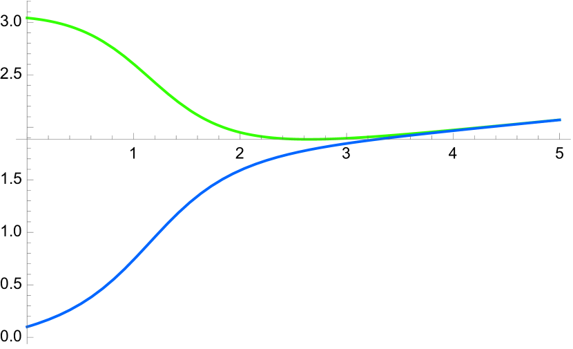
Refer to caption
(a) Example C.1: ϕ1(a)=ϕ2(a)=sin(a)+0.1subscriptitalic-ϕ1𝑎subscriptitalic-ϕ2𝑎𝑎0.1\phi_{1}(a)=\phi_{2}(a)=-\sin(a)+0.1.
Refer to caption
(b) Example C.2: ϕ1(a)=|sin(a/2)|subscriptitalic-ϕ1𝑎𝑎2\phi_{1}(a)=|\sin(a/2)|, ϕ2(a)=ϕ1(a)subscriptitalic-ϕ2𝑎subscriptitalic-ϕ1𝑎\phi_{2}(a)=-\phi_{1}(a)
Refer to caption
(c) Example C.3: ϕ1(a)=sin(a)subscriptitalic-ϕ1𝑎𝑎\phi_{1}(a)=\sin(a), ϕ2(a)=ϕ1(a)subscriptitalic-ϕ2𝑎subscriptitalic-ϕ1𝑎\phi_{2}(a)=-\phi_{1}(a)
Refer to caption
(d) Example C.4: ϕ1(a)=sin(2a)+2subscriptitalic-ϕ1𝑎2𝑎2\phi_{1}(a)=\sin(2a)+2, ϕ2(a)=sin(a)subscriptitalic-ϕ2𝑎𝑎\phi_{2}(a)=\sin(a)
Figure 3: Examples C (1 to 4).

5.2 Action of SO(3,)𝑆𝑂3SO(3,\mathbb{R}) on the sphere S2superscript𝑆2S^{2}

In this section, we describe population dynamics on the two-dimensional sphere S23superscript𝑆2superscript3S^{2}\subset\mathbb{R}^{3}. From now on, we consider a sphere S2superscript𝑆2S^{2} of radius 1. We use polar coordinates on the (x,y)𝑥𝑦(x,y) plane and mainly consider z>0𝑧0z>0 for the moment, i.e. we write

x=ρcos(θ),y=ρsin(θ),z=1ρ2.formulae-sequence𝑥𝜌𝜃formulae-sequence𝑦𝜌𝜃𝑧1superscript𝜌2x=\rho\cos(\theta),\qquad y=\rho\sin(\theta),\qquad z=\sqrt{1-\rho^{2}}.

We have two different groups that naturally act on the sphere. On one side, we consider the action of SO(3,)𝑆𝑂3SO(3,\mathbb{R}), that represents all rotations of the sphere. In the next Section 5.3, we will discuss the action of SO(2,)𝑆𝑂2SO(2,\mathbb{R}).

The Lie algebra so(3,)𝑠𝑜3so(3,\mathbb{R}) of SO(3,)𝑆𝑂3SO(3,\mathbb{R}), that are all rotations of 3superscript3\mathbb{R}^{3} around the zero, are as follows in the ρ,θ𝜌𝜃\rho,\theta-coordinates:

A=1ρ2(sin(θ)ρcos(θ)ρθ),B=1ρ2(cos(θ)ρsin(θ)ρθ),C=θ.formulae-sequence𝐴1superscript𝜌2𝜃subscript𝜌𝜃𝜌subscript𝜃formulae-sequence𝐵1superscript𝜌2𝜃subscript𝜌𝜃𝜌subscript𝜃𝐶subscript𝜃A=\sqrt{1-\rho^{2}}\left(-\sin(\theta)\partial_{\rho}-\frac{\cos(\theta)}{\rho}\partial_{\theta}\right),\qquad B=\sqrt{1-\rho^{2}}\left(\cos(\theta)\partial_{\rho}-\frac{\sin(\theta)}{\rho}\partial_{\theta}\right),\qquad C=\partial_{\theta}.

It holds [A,B]=C𝐴𝐵𝐶[A,B]=-C, [B,C]=A𝐵𝐶𝐴[B,C]=-A, [C,A]=B𝐶𝐴𝐵[C,A]=-B.

We now study the FPD in this case.

Proposition 42.

Consider the FPD associated to (N,S2,SO(3,))𝑁superscript𝑆2𝑆𝑂3(N,S^{2},SO(3,\mathbb{R})). Then:

  • 1.

    for N=1𝑁1N=1, the FPD is reduced to the null vector field;

  • 2.

    for N=2𝑁2N=2, all PDs are of the form

    F(X)=i=1Nfi(X)Xi with fi=ϕi,1(X)h(X1,X2)+ϕi,2(X)h(X1,X2),formulae-sequence𝐹𝑋superscriptsubscript𝑖1𝑁subscript𝑓𝑖𝑋subscriptsubscript𝑋𝑖 with subscript𝑓𝑖subscriptitalic-ϕ𝑖1𝑋subscript𝑋1subscript𝑋2subscriptitalic-ϕ𝑖2𝑋superscriptperpendicular-tosubscript𝑋1subscript𝑋2F(X)=\sum_{i=1}^{N}f_{i}(X)\partial_{X_{i}}\qquad\mbox{~{}~{} with ~{}~{}}\qquad f_{i}=\phi_{i,1}(X)h(X_{1},X_{2})+\phi_{i,2}(X)h^{\perp}(X_{1},X_{2}),

    where h(X1,X2)subscript𝑋1subscript𝑋2h(X_{1},X_{2}) is the component of the gradient of the Riemannian distance d(X1,X2)𝑑subscript𝑋1subscript𝑋2d(X_{1},X_{2}) on the variable X1subscript𝑋1X_{1} and hsuperscriptperpendicular-toh^{\perp} is its orthogonal on S2superscript𝑆2S^{2};

  • 3.

    for N3𝑁3N\geq 3, by choosing 3 distinct indexes k1,k2,k3subscript𝑘1subscript𝑘2subscript𝑘3k_{1},k_{2},k_{3}, all PDs are of the form

    F(X)=i=1Nfi(X)Xi with fi=ϕi,1(X)h(Xk1,Xk2)+ϕi,2(X)h(Xk1,Xk3),formulae-sequence𝐹𝑋superscriptsubscript𝑖1𝑁subscript𝑓𝑖𝑋subscriptsubscript𝑋𝑖 with subscript𝑓𝑖subscriptitalic-ϕ𝑖1𝑋subscript𝑋subscript𝑘1subscript𝑋subscript𝑘2subscriptitalic-ϕ𝑖2𝑋subscript𝑋subscript𝑘1subscript𝑋subscript𝑘3F(X)=\sum_{i=1}^{N}f_{i}(X)\partial_{X_{i}}\qquad\mbox{~{}~{} with ~{}~{}}\qquad f_{i}=\phi_{i,1}(X)h(X_{k_{1}},X_{k_{2}})+\phi_{i,2}(X)h(X_{k_{1}},X_{k_{3}}),

    where ϕi,k(X)subscriptitalic-ϕ𝑖𝑘𝑋\phi_{i,k}(X) are 𝔏^^𝔏\hat{\mathfrak{L}}-jointly radial functions of X=(X1,,XN)𝑋subscript𝑋1subscript𝑋𝑁X=(X_{1},\ldots,X_{N}) and h(Xa,Xb)subscript𝑋𝑎subscript𝑋𝑏h(X_{a},X_{b}) is the component of the gradient of the Riemannian distance d(Xa,Xb)𝑑subscript𝑋𝑎subscript𝑋𝑏d(X_{a},X_{b}) on the variable Xasubscript𝑋𝑎X_{a}.

Proof.

We first consider the case N=1𝑁1N=1. Let F𝐹F be a PD, whose domain is required to be open, dense and G𝐺G-invariant: since SO(3)𝑆𝑂3SO(3) acts transitively on S2superscript𝑆2S^{2}, its domain needs to be the whole S2superscript𝑆2S^{2}. Since S2superscript𝑆2S^{2} has Euler characteristic 2, then F𝐹F has at least one zero, i.e. F(X¯)=0𝐹¯𝑋0F(\bar{X})=0 for some X¯S2¯𝑋superscript𝑆2\bar{X}\in S^{2}. By equivariance of the vector field F𝐹F, all points in the orbit of X¯¯𝑋\bar{X} satisfy the same condition, i.e. F(gX¯)=0𝐹𝑔¯𝑋0F(g\bar{X})=0 for all gSO(3)𝑔𝑆𝑂3g\in SO(3). Since the action is transitive, we have F(X)=0𝐹𝑋0F(X)=0 for all XS2𝑋superscript𝑆2X\in S^{2}.

We now consider the case N=2𝑁2N=2. We have that hh is a solution, by recalling that the distance is radial and applying Proposition 24. It is easy to prove that the domain of hh is {X1±X2}subscript𝑋1plus-or-minussubscript𝑋2\{X_{1}\neq\pm X_{2}\}, that is G𝐺G-invariant and connected. Then, the definition of hsuperscriptperpendicular-toh^{\perp} is unique, up to a single change of sign. It is a solution, due to Corollary 25. It is easy to prove that it is independent on hh, thus h,hsuperscriptperpendicular-toh,h^{\perp} provide a basis of solutions for the 2-dimensional manifold. By Theorem 1, we have the result.

The case N3𝑁3N\geq 3 is a direct application of Corollary 26.

5.3 Action of SO(2,)𝑆𝑂2SO(2,\mathbb{R}) on the sphere S2superscript𝑆2S^{2}

In this section, we consider PDs on S2superscript𝑆2S^{2}, where the group action is SO(2,)𝑆𝑂2SO(2,\mathbb{R}), that is the Lie group of all rotations of 3superscript3\mathbb{R}^{3} around the z𝑧z-axis. In this example, the group of rotations preserves a specific axis: this is particularly interesting for models of swarms moving on the Earth that take into account the magnetic field, i.e. that preserve the Earth’s rotational axis passing through poles.

From now on, we consider the stereographic projection (x,y,z)(x1z,y1z)maps-to𝑥𝑦𝑧𝑥1𝑧𝑦1𝑧(x,y,z)\mapsto\left(\frac{x}{1-z},\frac{y}{1-z}\right), that is a diffeomorphism between the sphere without poles S2{(0,0,±1)}superscript𝑆200plus-or-minus1S^{2}\setminus\{(0,0,\pm 1)\} and the plane without the origin 2{0}superscript20\mathbb{R}^{2}\setminus\{0\}. Moreover, with this change of coordinates, the action of SO(2,)𝑆𝑂2SO(2,\mathbb{R}) on S2{(0,0,±1)}superscript𝑆200plus-or-minus1S^{2}\setminus\{(0,0,\pm 1)\} is identical to the classical one (rotations around the origin) on 2{0}superscript20\mathbb{R}^{2}\setminus\{0\}. We then represent equivariant trajectories on S2superscript𝑆2S^{2} by their stereographic projection, for simplicity of visualization.

Proposition 43.

Consider the FPD associated to (N,2{0},SO(2,))𝑁superscript20𝑆𝑂2(N,\mathbb{R}^{2}\setminus\{0\},SO(2,\mathbb{R})) with N1𝑁1N\geq 1, that is equivalent to the FPD associated to (N,S2{(0,0,±1)},SO(2,))𝑁superscript𝑆200plus-or-minus1𝑆𝑂2(N,S^{2}\setminus\{(0,0,\pm 1)\},SO(2,\mathbb{R})) by stereographic projection. Write Xi=(xi,yi)=ρi(cos(θi),sin(θi))subscript𝑋𝑖subscript𝑥𝑖subscript𝑦𝑖subscript𝜌𝑖subscript𝜃𝑖subscript𝜃𝑖X_{i}=(x_{i},y_{i})=\rho_{i}(\cos(\theta_{i}),\sin(\theta_{i})) on 2{0}superscript20\mathbb{R}^{2}\setminus\{0\} in Cartesian and polar coordinates.

PDs are of the form F=i=1Nfi,1xi+fi,2yi𝐹superscriptsubscript𝑖1𝑁subscript𝑓𝑖1subscriptsubscript𝑥𝑖subscript𝑓𝑖2subscriptsubscript𝑦𝑖F={\displaystyle\sum\limits_{i=1}^{N}}f_{i,1}\partial_{x_{i}}+f_{i,2}\partial_{y_{i}}, with

(fi,1fi,2)=(xiyiyixi)(ϕi(ρ1,,ρN,θ1θ2,,θ1θN)ψi(ρ1,,ρN,θ1θ2,,θ1θN)).subscript𝑓𝑖1subscript𝑓𝑖2subscript𝑥𝑖subscript𝑦𝑖subscript𝑦𝑖subscript𝑥𝑖subscriptitalic-ϕ𝑖subscript𝜌1subscript𝜌𝑁subscript𝜃1subscript𝜃2subscript𝜃1subscript𝜃𝑁subscript𝜓𝑖subscript𝜌1subscript𝜌𝑁subscript𝜃1subscript𝜃2subscript𝜃1subscript𝜃𝑁\left(\begin{array}[]{c}f_{i,1}\\ f_{i,2}\end{array}\right)=\left(\begin{array}[c]{cc}x_{i}&-y_{i}\\ y_{i}&x_{i}\end{array}\right)\left(\begin{array}[]{c}\phi_{i}(\rho_{1},\ldots,\rho_{N},\theta_{1}-\theta_{2},\ldots,\theta_{1}-\theta_{N})\\ \psi_{i}(\rho_{1},\ldots,\rho_{N},\theta_{1}-\theta_{2},\ldots,\theta_{1}-\theta_{N})\end{array}\right).
Proof.

Recall that the centralizer \mathfrak{C} of so(2,)𝑠𝑜2so(2,\mathbb{R}) is .Id+.Jformulae-sequenceId𝐽\mathbb{R}.\mathrm{Id}+\mathbb{R}.J with J𝐽J given by (2.16). Since \mathfrak{C} has dimension 2, thus one can apply Theorem 2, Item 1. The space of solutions is then given by ϕ(X)X+ψ(X)JXitalic-ϕ𝑋𝑋𝜓𝑋𝐽𝑋\phi(X)X+\psi(X)JX with ϕ(X),ψ(X)italic-ϕ𝑋𝜓𝑋\phi(X),\psi(X) being invariant with respect to the action of SO(2,)𝑆𝑂2SO(2,\mathbb{R}). By writing in polar coordinates Xi=ρi(cos(θi),sin(θi))subscript𝑋𝑖subscript𝜌𝑖subscript𝜃𝑖subscript𝜃𝑖X_{i}=\rho_{i}(\cos(\theta_{i}),\sin(\theta_{i})), one can apply a rotation of angle θ1subscript𝜃1-\theta_{1} and introduce the variables Yi=ρi(cos(θiθ1),sin(θiθ1))subscript𝑌𝑖subscript𝜌𝑖subscript𝜃𝑖subscript𝜃1subscript𝜃𝑖subscript𝜃1Y_{i}=\rho_{i}(\cos(\theta_{i}-\theta_{1}),\sin(\theta_{i}-\theta_{1})). Remark that, contrarily to the Euclidean case studied in Section 3, we still have the non-zero variable Y1=ρ1(1,0)subscript𝑌1subscript𝜌110Y_{1}=\rho_{1}(1,0). This implies that ϕ,ψitalic-ϕ𝜓\phi,\psi depend on variables ρ1,,ρN,θ2θ1,,θNθ1subscript𝜌1subscript𝜌𝑁subscript𝜃2subscript𝜃1subscript𝜃𝑁subscript𝜃1\rho_{1},\ldots,\rho_{N},\theta_{2}-\theta_{1},\ldots,\theta_{N}-\theta_{1}. ∎

Remark 44.

For N=1𝑁1N=1, we observe that the space of elementary solutions is strictly contained in the space of solutions, i.e. SSSS\mathcal{E}\subsetneq\SS. Indeed, it is reduced to solutions of the form ϕ(X)Xitalic-ϕ𝑋𝑋\phi(X)X. We are anyway able to completely characterize solutions, since 𝒞=SS𝒞SS\mathcal{C}=\SS, i.e. solutions given by the centralizer are all solutions.

For N2𝑁2N\geq 2, one can find alternative (equivalent) expressions for the PDs, by applying Theorem 2, Item 2.

We now show some examples of PDs associated to (N,2{0},SO(2,))𝑁superscript20𝑆𝑂2(N,\mathbb{R}^{2}\setminus\{0\},SO(2,\mathbb{R})) in the simple cases of N=1,2𝑁12N=1,2.

For N=1𝑁1N=1, in Figure 4-Left, we show four different examples of PDs, all starting from (x,y)=(1,1)𝑥𝑦11(x,y)=(1,1). We show that ϕ>0italic-ϕ0\phi>0 corresponds to move away from the origin, while ψ>0𝜓0\psi>0 corresponds to rotate counter-clockwise. Opposite signs mean opposite behavior. In particular, in Examples D.1, D.2 we have positive ϕitalic-ϕ\phi, with zero and negative ψ𝜓\psi, respectively. In Example D.3, we have ϕ0italic-ϕ0\phi\equiv 0 and ψ=10𝜓10\psi=10, providing a periodic circular trajectory with constant angular velocity. In Example D.4, we have ϕ(r)=24ritalic-ϕ𝑟24𝑟\phi(r)=2-4r, that provides stabilization of the radius to 0.50.50.5; at the same time, ψ=50>0𝜓500\psi=50>0 provides rotation with constant angular velocity. Example D.4, that has a nature similar to Example A.3 above, shows that one can stabilize the system towards a given radius (i.e. a given parallel on S2superscript𝑆2S^{2}). Instead, stabilization of the angular variable (or both radial and angular) is not achievable with such PDs, due to the invariance with respect to rotations.

For N=2𝑁2N=2, in Figure 4-Right we show three different examples of PDs, in which agent 1 is marked in green and agent 2 is marked in blue. Similarly to the previous case, we can have convergence of both the radius and angular variables (Example E.1), eventually choosing the radius (Example E.2, the target radius being r=2𝑟2r=2). One can also converge to a chosen angular difference (Example E.3, angular difference π/8𝜋8\pi/8), but cannot send agents to a chosen common angle. We explicitly have the following choices of functional parameters:

Example E.1

ϕ1=ρ2ρ1=ϕ2subscriptitalic-ϕ1subscript𝜌2subscript𝜌1subscriptitalic-ϕ2\phi_{1}=\rho_{2}-\rho_{1}=-\phi_{2}, ψ1=sin(θ2θ1)=ψ2subscript𝜓1subscript𝜃2subscript𝜃1subscript𝜓2\psi_{1}=\sin(\theta_{2}-\theta_{1})=-\psi_{2}.

Example E.2

ϕ1=2ρ1subscriptitalic-ϕ12subscript𝜌1\phi_{1}=2-\rho_{1}, ϕ2=2ρ2subscriptitalic-ϕ22subscript𝜌2\phi_{2}=2-\rho_{2}, ψ1=sin(θ2θ1)=ψ2subscript𝜓1subscript𝜃2subscript𝜃1subscript𝜓2\psi_{1}=\sin(\theta_{2}-\theta_{1})=-\psi_{2}.

Example E.3

ϕ1=0.1subscriptitalic-ϕ10.1\phi_{1}=0.1, ϕ2=ρ1ρ2subscriptitalic-ϕ2subscript𝜌1subscript𝜌2\phi_{2}=\rho_{1}-\rho_{2}, ψ1=sin(θ2θ1π/8)=ψ2subscript𝜓1subscript𝜃2subscript𝜃1𝜋8subscript𝜓2\psi_{1}=\sin(\theta_{2}-\theta_{1}-\pi/8)=-\psi_{2}.

Refer to caption
(a) Examples D (1 to 4).
Refer to caption
(b) Examples E (1 to 3).
Figure 4: Examples on S2superscript𝑆2S^{2} with N=1𝑁1N=1 and N=2𝑁2N=2.

6 Volume preserving Population Dynamics on the plane

In this section, we consider Population Dynamics on the punctured plane 2{0}superscript20\mathbb{R}^{2}\setminus\{0\} under the action of SL(2)𝑆𝐿2SL(2). The case is interesting, since it is the only one, among our examples, in which the group is not a group of isometries (or pseudo-isometries).

The resulting dynamics on the punctured plane 2{0}superscript20\mathbb{R}^{2}\setminus\{0\} preserve volumes: given two points X1=(x1,y1)subscript𝑋1subscript𝑥1subscript𝑦1X_{1}=(x_{1},y_{1}) and X2=(x2,y2)subscript𝑋2subscript𝑥2subscript𝑦2X_{2}=(x_{2},y_{2}), we denote by

X1X2:=|x1x2y1y2|=x1y2y1x2assignsubscript𝑋1subscript𝑋2subscript𝑥1subscript𝑥2subscript𝑦1subscript𝑦2subscript𝑥1subscript𝑦2subscript𝑦1subscript𝑥2X_{1}\wedge X_{2}:=\left|\begin{array}[]{cc}x_{1}&x_{2}\\ y_{1}&y_{2}\end{array}\right|=x_{1}y_{2}-y_{1}x_{2}

the (oriented) area of the parallelogram with vertices 0,X1,X1+X2,X20subscript𝑋1subscript𝑋1subscript𝑋2subscript𝑋20,X_{1},X_{1}+X_{2},X_{2}. It is easy to prove that volumes are preserved by the action of the special linear group SL(2,)𝑆𝐿2SL(2,\mathbb{R}) composed of matrices with determinant 1.

We now describe jointly radial functions and PDs for the action of SL(2)𝑆𝐿2SL(2).

Proposition 45.

Let M=2{0}𝑀superscript20M=\mathbb{R}^{2}\setminus\{0\}. Consider the set 𝒪={X1X20}MN𝒪subscript𝑋1subscript𝑋20superscript𝑀𝑁\mathcal{O}=\{X_{1}\wedge X_{2}\neq 0\}\subset M^{N}, that it is open dense, G𝐺G-invariant.

The jointly radial functions on MNsuperscript𝑀𝑁M^{N} defined on 𝒪𝒪\mathcal{O} are

ψ(X1,,XN)=ϕ(X1X2,[X1|X2]1X3,,[X1|X2]1XN),𝜓subscript𝑋1subscript𝑋𝑁italic-ϕsubscript𝑋1subscript𝑋2superscriptdelimited-[]conditionalsubscript𝑋1subscript𝑋21subscript𝑋3superscriptdelimited-[]conditionalsubscript𝑋1subscript𝑋21subscript𝑋𝑁\psi(X_{1},\ldots,X_{N})=\phi(X_{1}\wedge X_{2},[X_{1}|X_{2}]^{-1}X_{3},\ldots,[X_{1}|X_{2}]^{-1}X_{N}), (6.1)

where [X1|X2]delimited-[]conditionalsubscript𝑋1subscript𝑋2[X_{1}|X_{2}] is the 2×2222\times 2-matrix with columns given by X1,X2subscript𝑋1subscript𝑋2X_{1},X_{2} and ϕitalic-ϕ\phi is an analytic function of its N2𝑁2N-2 variables in 2superscript2\mathbb{R}^{2}. Consider now the FPD associated to (N,,SL(2,))(N,,SL(2,\mathbb{R})).

  • 1.

    For N=1𝑁1N=1, all PDs are of the form F=α(x1x1+y1y1)𝐹𝛼subscript𝑥1subscriptsubscript𝑥1subscript𝑦1subscriptsubscript𝑦1F=\alpha\left(x_{1}\partial_{x_{1}}+y_{1}\partial_{y_{1}}\right) for α𝛼\alpha\in\mathbb{R}.

  • 2.

    For N2𝑁2N\geq 2, choose two distinct indexes j1,j2{1,,N}subscript𝑗1subscript𝑗21𝑁j_{1},j_{2}\in\{1,\ldots,N\}. Then, all PDs are of the form

    F=i=1Nϕ1,i(xj1xi+yj1yi)+ϕ2,i(xj2xi+yj2yi)𝐹superscriptsubscript𝑖1𝑁subscriptitalic-ϕ1𝑖subscript𝑥subscript𝑗1subscriptsubscript𝑥𝑖subscript𝑦subscript𝑗1subscriptsubscript𝑦𝑖subscriptitalic-ϕ2𝑖subscript𝑥subscript𝑗2subscriptsubscript𝑥𝑖subscript𝑦subscript𝑗2subscriptsubscript𝑦𝑖F=\sum_{i=1}^{N}\phi_{1,i}\left(x_{j_{1}}\partial_{x_{i}}+y_{j_{1}}\partial_{y_{i}}\right)+\phi_{2,i}\left(x_{j_{2}}\partial_{x_{i}}+y_{j_{2}}\partial_{y_{i}}\right)

    where ϕi,1,ϕi,2subscriptitalic-ϕ𝑖1subscriptitalic-ϕ𝑖2\phi_{i,1},\phi_{i,2} are arbitrary jointly-radial functions, i.e. of the form (6.1).

Proof.

We first prove that jointly radial functions are of the form (6.1). It is easy to prove that ψ𝜓\psi of such form is jointly equivariant: the diagonal action of gSL(2)𝑔𝑆𝐿2g\in SL(2) reads as

ψ(gX1,,gXN)𝜓𝑔subscript𝑋1𝑔subscript𝑋𝑁\displaystyle\psi(gX_{1},\ldots,gX_{N}) =\displaystyle= ϕ((gX1)(gX2),[gX1|gX2]1(gX3),,[gX1|gX2]1gXN)italic-ϕ𝑔subscript𝑋1𝑔subscript𝑋2superscriptdelimited-[]conditional𝑔subscript𝑋1𝑔subscript𝑋21𝑔subscript𝑋3superscriptdelimited-[]conditional𝑔subscript𝑋1𝑔subscript𝑋21𝑔subscript𝑋𝑁\displaystyle\phi((gX_{1})\wedge(gX_{2}),[gX_{1}|gX_{2}]^{-1}(gX_{3}),\ldots,[gX_{1}|gX_{2}]^{-1}gX_{N})
=\displaystyle= ϕ(X1X2,[X1|X2]1X3,,[X1|X2]1XN)=ψ(X1,,XN).italic-ϕsubscript𝑋1subscript𝑋2superscriptdelimited-[]conditionalsubscript𝑋1subscript𝑋21subscript𝑋3superscriptdelimited-[]conditionalsubscript𝑋1subscript𝑋21subscript𝑋𝑁𝜓subscript𝑋1subscript𝑋𝑁\displaystyle\phi(X_{1}\wedge X_{2},[X_{1}|X_{2}]^{-1}X_{3},\ldots,[X_{1}|X_{2}]^{-1}X_{N})=\psi(X_{1},\ldots,X_{N}).

Here we used that the determinant is invariant under the action of g𝑔g and that

[gX1|gX2]1gXi=[X1|X2]1g1gXi=[X1|X2]1Xi.superscriptdelimited-[]conditional𝑔subscript𝑋1𝑔subscript𝑋21𝑔subscript𝑋𝑖superscriptdelimited-[]conditionalsubscript𝑋1subscript𝑋21superscript𝑔1𝑔subscript𝑋𝑖superscriptdelimited-[]conditionalsubscript𝑋1subscript𝑋21subscript𝑋𝑖[gX_{1}|gX_{2}]^{-1}gX_{i}=[X_{1}|X_{2}]^{-1}g^{-1}gX_{i}=[X_{1}|X_{2}]^{-1}X_{i}.

It is clear that all jointly radial functions are of this form, since the variables in (6.1) play the role of coordinates in the quotient 𝒪/G𝒪𝐺\mathcal{O}/G.

We now study the case N=1𝑁1N=1. Let F𝐹F be a PD, which domain is a G𝐺G-space. Since SL(2,)𝑆𝐿2SL(2,\mathbb{R}) acts transitively on M𝑀M, its domain is the whole M𝑀M. Write F(X)=f(x,y)x+g(x,y)y𝐹𝑋𝑓𝑥𝑦subscript𝑥𝑔𝑥𝑦subscript𝑦F(X)=f(x,y)\partial_{x}+g(x,y)\partial_{y} and write [F,l]=0𝐹𝑙0[F,l]=0 for l𝑙l in the basis of the Lie algebra so(2,)𝑠𝑜2so(2,\mathbb{R}), that is

l1=yx,l2=xy,l3=xxyy.formulae-sequencesubscript𝑙1𝑦subscript𝑥formulae-sequencesubscript𝑙2𝑥subscript𝑦subscript𝑙3𝑥subscript𝑥𝑦subscript𝑦l_{1}=y\partial_{x},\qquad l_{2}=x\partial_{y},\qquad l_{3}=x\partial_{x}-y\partial_{y}.

A direct computation shows:

[F,l1]=gxy(xf)xy(xg)y,[F,l2]=fyx(yf)xx(yg)y.formulae-sequence𝐹subscript𝑙1𝑔subscript𝑥𝑦subscript𝑥𝑓subscript𝑥𝑦subscript𝑥𝑔subscript𝑦𝐹subscript𝑙2𝑓subscript𝑦𝑥subscript𝑦𝑓subscript𝑥𝑥subscript𝑦𝑔subscript𝑦[F,l_{1}]=g\partial_{x}-y(\partial_{x}f)\partial_{x}-y(\partial_{x}g)\partial_{y},\qquad[F,l_{2}]=f\partial_{y}-x(\partial_{y}f)\partial_{x}-x(\partial_{y}g)\partial_{y}.

This implies that g=g(y)𝑔𝑔𝑦g=g(y) and f=f(x)𝑓𝑓𝑥f=f(x). Since g(y)=yxf𝑔𝑦𝑦subscript𝑥𝑓g(y)=y\partial_{x}f, then g=ky𝑔𝑘𝑦g=ky for some k𝑘k\in\mathbb{R}. Similarly, f=kx𝑓𝑘𝑥f=kx for the same k𝑘k. By linearity, we are now left to prove that F(x)=xx+yy𝐹𝑥𝑥subscript𝑥𝑦subscript𝑦F(x)=x\partial_{x}+y\partial_{y} satisfies

[F,l3]=(xxyy)(xxyy)=0.𝐹subscript𝑙3𝑥subscript𝑥𝑦subscript𝑦𝑥subscript𝑥𝑦subscript𝑦0[F,l_{3}]=(x\partial_{x}-y\partial_{y})-(x\partial_{x}-y\partial_{y})=0.

This proves the result.

The case N2𝑁2N\geq 2 is a direct application of Theorem 2, Item 2. ∎

7 Controlled Population Dynamics: the unicycle

In this section, we describe an interesting problem of Controlled Population Dynamics as given in Definition 11, i.e. a PD in which the dynamics is constrained to belong to a subset ΩΩ\Omega of the Lie algebra of vector fields. In the terminology of mechanical systems, constraints on the velocity are known as non-holonomic.

7.1 The classical unicycle

The unicycle is a classical model of a vehicle on the plane 2superscript2\mathbb{R}^{2} moving along straight lines or turning on itself, or combine these displacements. The state space is then 2×S1superscript2superscript𝑆1\mathbb{R}^{2}\times S^{1}, i.e. the state is described by the position-orientation variables (x,y,θ)𝑥𝑦𝜃(x,y,\theta). The dynamics is given by

x˙=cos(θ)u(t),y˙=sin(θ)u(t),θ˙=v(t).formulae-sequence˙𝑥𝜃𝑢𝑡formulae-sequence˙𝑦𝜃𝑢𝑡˙𝜃𝑣𝑡\dot{x}=\cos(\theta)u(t),\qquad\dot{y}=\sin(\theta)u(t),\qquad\dot{\theta}=v(t). (7.1)

Here, u(t),v(t)𝑢𝑡𝑣𝑡u(t),v(t) are the control variables, accounting for straight movements and rotations, respectively. Remark that the constraint is linear, since ΩΩ\Omega is generated by F1=cos(θ)x+sin(θ)y,F2=θformulae-sequencesubscript𝐹1𝜃subscript𝑥𝜃subscript𝑦subscript𝐹2subscript𝜃F_{1}=\cos(\theta)\partial_{x}+\sin(\theta)\partial_{y},F_{2}=\partial_{\theta}. It is not a Lie algebra, since it holds [F1,F2]=sin(θ)x+cos(θ)yΩsubscript𝐹1subscript𝐹2𝜃subscript𝑥𝜃subscript𝑦Ω[F_{1},F_{2}]=-\sin(\theta)\partial_{x}+\cos(\theta)\partial_{y}\not\in\Omega.

One of the interests of this model in the context of PDs is that it is a first-order system that allows to describe orientation of the displacements (via the variable θ𝜃\theta). This is in sharp contrast with other models, such as the celebrated Cucker-Smale model [14], in which orientation is encoded by a second-order dynamics. Clearly, the advantage of dealing with first-order systems is here mitigated by the non-holonomic constraint.

We now impose equivariance with respect to the action of the group G=SE(2)𝐺𝑆𝐸2G=SE(2) of rototranslation of the plane. The action on 2×S1superscript2superscript𝑆1\mathbb{R}^{2}\times S^{1} is the following: given an element

g=(cos(τ)sin(τ)asin(τ)cos(τ)b001)SE(2)𝑔𝜏𝜏𝑎𝜏𝜏𝑏001𝑆𝐸2g=\left(\begin{array}[]{ccc}\cos(\tau)&-\sin(\tau)&a\\ \sin(\tau)&\cos(\tau)&b\\ 0&0&1\end{array}\right)\in SE(2)

and (x,y,θ)2×S1𝑥𝑦𝜃superscript2superscript𝑆1(x,y,\theta)\in\mathbb{R}^{2}\times S^{1}, it holds

Φ(g)(xyθ)=(cos(τ)sin(τ)0sin(τ)cos(τ)0001)(xyθ)+(abτ).Φ𝑔𝑥𝑦𝜃𝜏𝜏0𝜏𝜏0001𝑥𝑦𝜃𝑎𝑏𝜏\Phi(g)\left(\begin{array}[]{c}x\\ y\\ \theta\end{array}\right)=\left(\begin{array}[]{ccc}\cos(\tau)&-\sin(\tau)&0\\ \sin(\tau)&\cos(\tau)&0\\ 0&0&1\end{array}\right)\left(\begin{array}[]{c}x\\ y\\ \theta\end{array}\right)+\left(\begin{array}[]{c}a\\ b\\ \tau\end{array}\right). (7.2)

The Lie algebra 𝔏𝔏\mathfrak{L} is then generated by the 3 vector fields {x,y,yx+xy+θ}subscript𝑥subscript𝑦𝑦subscript𝑥𝑥subscript𝑦subscript𝜃\left\{\partial_{x},\partial_{y},-y\partial_{x}+x\partial_{y}+\partial_{\theta}\right\}. The equation (7.1) is the differential equation associated with left-invariant vector fields, while (7.2) is associated with right-invariant vector field (i.e. left translations).

We are now ready to describe the Controlled FPD for the unycicle.

Proposition 46.

Consider the Family of CPD associated to (N,2×S1,SO(2,)2,Ω)𝑁superscript2superscript𝑆1left-normal-factor-semidirect-product𝑆𝑂2superscript2Ω(N,\mathbb{R}^{2}\times S^{1},SO(2,\mathbb{R})\ltimes\mathbb{R}^{2},\Omega) with N1𝑁1N\geq 1 and ΩΩ\Omega given by (7.1). Denote by Xi=(xi,yi,θi)subscript𝑋𝑖subscript𝑥𝑖subscript𝑦𝑖subscript𝜃𝑖X_{i}=(x_{i},y_{i},\theta_{i}) the state of the i𝑖i-th agent and X:=(X1,,XN)assign𝑋subscript𝑋1subscript𝑋𝑁X:=(X_{1},\ldots,X_{N}). Let

X˙i=ui(X)Fi+vi(X)Gi with Fi=cos(θi)xi+sin(θi)yi and Gi=θi.formulae-sequencesubscript˙𝑋𝑖subscript𝑢𝑖𝑋subscript𝐹𝑖subscript𝑣𝑖𝑋subscript𝐺𝑖 with formulae-sequencesubscript𝐹𝑖subscript𝜃𝑖subscriptsubscript𝑥𝑖subscript𝜃𝑖subscriptsubscript𝑦𝑖 and subscript𝐺𝑖subscriptsubscript𝜃𝑖\dot{X}_{i}=u_{i}(X)F_{i}+v_{i}(X)G_{i}\qquad\qquad\mbox{ with }\qquad F_{i}=\cos(\theta_{i})\partial_{x_{i}}+\sin(\theta_{i})\partial_{y_{i}}\quad\mbox{~{}~{} and ~{}~{}}\quad G_{i}=\partial_{\theta_{i}}.

Then, the controlled FPD is characterized by the fact that ui,visubscript𝑢𝑖subscript𝑣𝑖u_{i},v_{i} are analytic functions of ρ2,,ρNsubscript𝜌2subscript𝜌𝑁\rho_{2},\ldots,\rho_{N}, α2θ1,,αNθ1,θ2θ1,,θNθ1subscript𝛼2subscript𝜃1subscript𝛼𝑁subscript𝜃1subscript𝜃2subscript𝜃1subscript𝜃𝑁subscript𝜃1\alpha_{2}-\theta_{1},\ldots,\alpha_{N}-\theta_{1},\theta_{2}-\theta_{1},\ldots,\theta_{N}-\theta_{1} only, where Zi:=(xix1,yiy1)=ρi(cos(αi),sin(αi))assignsubscript𝑍𝑖subscript𝑥𝑖subscript𝑥1subscript𝑦𝑖subscript𝑦1subscript𝜌𝑖subscript𝛼𝑖subscript𝛼𝑖Z_{i}:=(x_{i}-x_{1},y_{i}-y_{1})=\rho_{i}(\cos(\alpha_{i}),\sin(\alpha_{i})) for i=2,,N𝑖2𝑁i=2,\ldots,N.

Proof.

We identify the unicycle variables (x,y,θ)𝑥𝑦𝜃(x,y,\theta) with the element XSE(2)𝑋𝑆𝐸2X\in SE(2) defined by

X=(cos(θ)sin(θ)xsin(θ)cos(θ)y001).𝑋𝜃𝜃𝑥𝜃𝜃𝑦001X=\left(\begin{array}[]{ccc}\cos(\theta)&-\sin(\theta)&x\\ \sin(\theta)&\cos(\theta)&y\\ 0&0&1\end{array}\right).

The action described in (7.2) can be rewritten as Φ(g)X=gXΦ𝑔𝑋𝑔𝑋\Phi(g)X=gX, i.e. it is a left translation on SE(2)𝑆𝐸2SE(2). We can now study FPD on SE(2)𝑆𝐸2SE(2) without the constraint, that are completely characterized by Proposition 23. Indeed, the FPD is given by

X˙i=j=13ψij(X1,,XN)(Xilj),subscript˙𝑋𝑖superscriptsubscript𝑗13subscript𝜓𝑖𝑗subscript𝑋1subscript𝑋𝑁subscript𝑋𝑖superscript𝑙𝑗\dot{X}_{i}=\sum_{j=1}^{3}\psi_{ij}(X_{1},\ldots,X_{N})(X_{i}\cdot l^{j}), (7.3)

where l1,l2,l3superscript𝑙1superscript𝑙2superscript𝑙3l^{1},l^{2},l^{3} is a basis of the Lie algebra, hence Xl1,Xl2,Xl3𝑋superscript𝑙1𝑋superscript𝑙2𝑋superscript𝑙3X\cdot l^{1},X\cdot l^{2},X\cdot l^{3} is a basis of the left-invariant vector fields. Such a basis can be chosen as

l1=(001000000),l2=(010100000),l3=(000001000).formulae-sequencesuperscript𝑙1001000000formulae-sequencesuperscript𝑙2010100000superscript𝑙3000001000l^{1}=\left(\begin{array}[]{ccc}0&0&1\\ 0&0&0\\ 0&0&0\end{array}\right),\qquad l^{2}=\left(\begin{array}[]{ccc}0&-1&0\\ 1&0&0\\ 0&0&0\end{array}\right),\qquad l^{3}=\left(\begin{array}[]{ccc}0&0&0\\ 0&0&1\\ 0&0&0\end{array}\right). (7.4)

Moreover, the ψij(X1,,XN)subscript𝜓𝑖𝑗subscript𝑋1subscript𝑋𝑁\psi_{ij}(X_{1},\ldots,X_{N}) are jointly radial. Again by Proposition 23, they are characterized by the fact that they are analytic functions of ρ2,,ρNsubscript𝜌2subscript𝜌𝑁\rho_{2},\ldots,\rho_{N}, α2θ1,,αNθ1,θ2θ1,,θNθ1subscript𝛼2subscript𝜃1subscript𝛼𝑁subscript𝜃1subscript𝜃2subscript𝜃1subscript𝜃𝑁subscript𝜃1\alpha_{2}-\theta_{1},\ldots,\alpha_{N}-\theta_{1},\theta_{2}-\theta_{1},\ldots,\theta_{N}-\theta_{1} only, where Zi:=(xix1,yiy1)=ρi(cos(αi),sin(αi))assignsubscript𝑍𝑖subscript𝑥𝑖subscript𝑥1subscript𝑦𝑖subscript𝑦1subscript𝜌𝑖subscript𝛼𝑖subscript𝛼𝑖Z_{i}:=(x_{i}-x_{1},y_{i}-y_{1})=\rho_{i}(\cos(\alpha_{i}),\sin(\alpha_{i})) for i=2,,N𝑖2𝑁i=2,\ldots,N.

We now identify the Controlled Population Dynamics, by simply verifying which dynamics for the unicycle (7.1) are of the form (7.3). Observe that (7.1) reads as X˙=u(t)F1(X)+v(t)F2(X)˙𝑋𝑢𝑡subscript𝐹1𝑋𝑣𝑡subscript𝐹2𝑋\dot{X}=u(t)F_{1}(X)+v(t)F_{2}(X) and that F1(X)=Xl1subscript𝐹1𝑋𝑋superscript𝑙1F_{1}(X)=X\cdot l^{1}, F2(X)=Xl2subscript𝐹2𝑋𝑋superscript𝑙2F_{2}(X)=X\cdot l^{2}. As a consequence, solutions of the unicycle (7.1) are of the form (7.3) if and only if ψi30subscript𝜓𝑖30\psi_{i3}\equiv 0. This proves the result. ∎

We now discuss examples. For N=1𝑁1N=1, controls u,v𝑢𝑣u,v need to be constant, hence providing circular trajectories (that we do not present here). We provide a single example for N=2𝑁2N=2 in Figure 5, where u1=0.3ρ2,v1=.2sin(θ1α2),u2=0.2ρ2,v2=0.1ρ2formulae-sequencesubscript𝑢10.3subscript𝜌2formulae-sequencesubscript𝑣1.2subscript𝜃1subscript𝛼2formulae-sequencesubscript𝑢20.2subscript𝜌2subscript𝑣20.1subscript𝜌2u_{1}=0.3\rho_{2},v_{1}=-.2\sin(\theta_{1}-\alpha_{2}),u_{2}=0.2\rho_{2},v_{2}=-0.1\rho_{2}. With such choice, agent 1 (green) aims to reach agent 2 (blue) with the same angle. Moreover, the dynamics promotes convergence to an equilibrium, in which ρ2=0subscript𝜌20\rho_{2}=0.

Refer to caption
Figure 5: A Controlled Population Dynamics for the unicycle with N=2𝑁2N=2.

7.2 The relativistic unicycle

In this section, we consider a unicycle in space-time, by adding the time variable T𝑇T. The dynamics then takes place in 3×S1superscript3superscript𝑆1\mathbb{R}^{3}\times S^{1} and it can be written as follows:

T˙=f(t),x˙=cos(θ)u(t),y˙=sin(θ)u(t),θ˙=v(t).formulae-sequence˙𝑇𝑓𝑡formulae-sequence˙𝑥𝜃𝑢𝑡formulae-sequence˙𝑦𝜃𝑢𝑡˙𝜃𝑣𝑡\dot{T}=f(t),\qquad\dot{x}=\cos(\theta)u(t),\qquad\dot{y}=\sin(\theta)u(t),\qquad\dot{\theta}=v(t). (7.5)

The natural group of equivariance for the variables (T,x,y)𝑇𝑥𝑦(T,x,y) only is the group SO(1,2)3left-normal-factor-semidirect-product𝑆𝑂12superscript3SO(1,2)\ltimes\mathbb{R}^{3}, that we already studied in Section 4.2. No natural action of such group seems to take into account the non-holonomic angular constraint for (x,y,θ)𝑥𝑦𝜃(x,y,\theta) in (7.5).

A natural group of equivariance is K=SO(1,1)×SO(2,)𝐾𝑆𝑂11𝑆𝑂2K=SO(1,1)\times SO(2,\mathbb{R}), acting as follows: by introducing polar coordinates for (x,y)=ρ(cos(α),sin(α))𝑥𝑦𝜌𝛼𝛼(x,y)=\rho(\cos(\alpha),\sin(\alpha)), the action is (g,ω).(T,ρ,α,θ)=(g.(T,ρ),α+ω,θ+ω)(g,\omega).(T,\rho,\alpha,\theta)=(g.(T,\rho),\alpha+\omega,\theta+\omega), where gSO(1,1)𝑔𝑆𝑂11g\in SO(1,1) is written as g=(cosh(λ)sinh(λ)sinh(λ)cosh(λ))𝑔𝜆𝜆𝜆𝜆g=\left(\begin{array}[c]{cc}\cosh(\lambda)&\sinh(\lambda)\\ \sinh(\lambda)&\cosh(\lambda)\end{array}\right). The action can be seen as the natural “Lorentzian” group action, as it preserves the metric ds2=dT2dρ2𝑑superscript𝑠2𝑑superscript𝑇2𝑑superscript𝜌2ds^{2}=dT^{2}-d\rho^{2}. The rotation ω𝜔\omega simultaneously acts on the variables α𝛼\alpha and θ𝜃\theta. We have the following result.

Proposition 47.

Consider the controlled FPD associated to the relativistic unicycle (N,3×S1,SO(1,1)×SO(2,))𝑁superscript3superscript𝑆1𝑆𝑂11𝑆𝑂2(N,\mathbb{R}^{3}\times S^{1},SO(1,1)\times SO(2,\mathbb{R})).

For N=1𝑁1N=1, the controlled FPD is composed by vector fields

Tcos(θα)u¯(r,θα)T+ρcos(θα)u¯(r,θα)ρ+sin(θα)u¯(r,θα)α+v(r,θα)θ𝑇𝜃𝛼¯𝑢𝑟𝜃𝛼subscript𝑇𝜌𝜃𝛼¯𝑢𝑟𝜃𝛼subscript𝜌𝜃𝛼¯𝑢𝑟𝜃𝛼subscript𝛼𝑣𝑟𝜃𝛼subscript𝜃T\cos(\theta-\alpha)\bar{u}(r,\theta-\alpha)\partial_{T}+\rho\cos(\theta-\alpha)\bar{u}(r,\theta-\alpha)\partial_{\rho}+\sin(\theta-\alpha)\bar{u}(r,\theta-\alpha)\partial_{\alpha}+v(r,\theta-\alpha)\partial_{\theta} (7.6)

with u¯,v¯𝑢𝑣\bar{u},v analytic functions and r=T2ρ2𝑟superscript𝑇2superscript𝜌2r=\sqrt{T^{2}-\rho^{2}}.

For N2𝑁2N\geq 2, the FPD contains vector fields F=i=1NFiXi𝐹superscriptsubscript𝑖1𝑁subscript𝐹𝑖subscriptsubscript𝑋𝑖F=\sum_{i=1}^{N}F_{i}\partial_{X_{i}} with

Fisubscript𝐹𝑖\displaystyle F_{i} =\displaystyle= Ticos(θiαi)u¯i(X1,,XN)Ti+ρicos(θiαi)u¯i(X1,,XN)ρi+subscript𝑇𝑖subscript𝜃𝑖subscript𝛼𝑖subscript¯𝑢𝑖subscript𝑋1subscript𝑋𝑁subscriptsubscript𝑇𝑖limit-fromsubscript𝜌𝑖subscript𝜃𝑖subscript𝛼𝑖subscript¯𝑢𝑖subscript𝑋1subscript𝑋𝑁subscriptsubscript𝜌𝑖\displaystyle T_{i}\cos(\theta_{i}-\alpha_{i})\bar{u}_{i}(X_{1},\ldots,X_{N})\partial_{T_{i}}+\rho_{i}\cos(\theta_{i}-\alpha_{i})\bar{u}_{i}(X_{1},\ldots,X_{N})\partial_{\rho_{i}}+
sin(θiαi)u¯i(X1,,XN)αi+v¯i(X1,,XN)θi,subscript𝜃𝑖subscript𝛼𝑖subscript¯𝑢𝑖subscript𝑋1subscript𝑋𝑁subscriptsubscript𝛼𝑖subscript¯𝑣𝑖subscript𝑋1subscript𝑋𝑁subscriptsubscript𝜃𝑖\displaystyle\sin(\theta_{i}-\alpha_{i})\bar{u}_{i}(X_{1},\ldots,X_{N})\partial_{\alpha_{i}}+\bar{v}_{i}(X_{1},\ldots,X_{N})\partial_{\theta_{i}},

where u¯i,v¯isubscript¯𝑢𝑖subscript¯𝑣𝑖\bar{u}_{i},\bar{v}_{i} are jointly radial functions of their variables.

Proof.

We first focus on N=1𝑁1N=1. We use polar coordinates for (x,y)=ρ(cos(α),sin(α))𝑥𝑦𝜌𝛼𝛼(x,y)=\rho(\cos(\alpha),\sin(\alpha)). The system reads as

T˙=f(T,ρ,α,θ),ρ˙=cos(θα)u(T,ρ,α,θ),α˙=1ρsin(θα)u(T,ρ,α,θ),θ˙=v(T,ρ,α,θ).formulae-sequence˙𝑇𝑓𝑇𝜌𝛼𝜃formulae-sequence˙𝜌𝜃𝛼𝑢𝑇𝜌𝛼𝜃formulae-sequence˙𝛼1𝜌𝜃𝛼𝑢𝑇𝜌𝛼𝜃˙𝜃𝑣𝑇𝜌𝛼𝜃\dot{T}=f(T,\rho,\alpha,\theta),\qquad\dot{\rho}=\cos(\theta-\alpha)u(T,\rho,\alpha,\theta),\qquad\dot{\alpha}=\frac{1}{\rho}\sin(\theta-\alpha)u(T,\rho,\alpha,\theta),\qquad\dot{\theta}=v(T,\rho,\alpha,\theta).

The action of SO(2,)𝑆𝑂2SO(2,\mathbb{R}) implies that the dynamics depends on the variables T,ρ,θα𝑇𝜌𝜃𝛼T,\rho,\theta-\alpha only, thus f,u,v𝑓𝑢𝑣f,u,v only depend on them.

The action of SO(1,1)𝑆𝑂11SO(1,1) implies two conditions: first, that functions f,u,v𝑓𝑢𝑣f,u,v depend on the variables r,θα𝑟𝜃𝛼r,\theta-\alpha only, with r=T2ρ2𝑟superscript𝑇2superscript𝜌2r=\sqrt{T^{2}-\rho^{2}}. Second, it implies f(T,ρ,θα)=ψ(r,θα)T𝑓𝑇𝜌𝜃𝛼𝜓𝑟𝜃𝛼𝑇f(T,\rho,\theta-\alpha)=\psi(r,\theta-\alpha)T and cos(θα)u(T,ρ,θα)=ψ(r,θα)ρ𝜃𝛼𝑢𝑇𝜌𝜃𝛼𝜓𝑟𝜃𝛼𝜌\cos(\theta-\alpha)u(T,\rho,\theta-\alpha)=\psi(r,\theta-\alpha)\rho for an analytic function ψ(r,θα)𝜓𝑟𝜃𝛼\psi(r,\theta-\alpha). Computations are identical to the proof of Proposition 39 with N=2𝑁2N=2. We now write ψ(r,θα)=cos(θα)u¯(r,θα)𝜓𝑟𝜃𝛼𝜃𝛼¯𝑢𝑟𝜃𝛼\psi(r,\theta-\alpha)=\cos(\theta-\alpha)\bar{u}(r,\theta-\alpha) for an analytic function u¯(r,θα)=u(t)ρ¯𝑢𝑟𝜃𝛼𝑢𝑡𝜌\bar{u}(r,\theta-\alpha)=\frac{u(t)}{\rho} and find (7.6).

For N2𝑁2N\geq 2, it is easy to prove that F𝐹F defined by (47) are PD, with the same computations. ∎

8 Population Dynamics for quantum agents

In this section, we discuss the problem of joint equivariance of systems of quantum particles. In the standard formalism of quantum theory (see e.g. [33]), particles are described by (square roots of) probability densities. We consider a finite-dimensional dynamics, i.e. n𝑛n\in\mathbb{N} possible states. The Schrödinger equation describing the evolution of a single particle is then:

Ψ˙=AΨ,˙Ψ𝐴Ψ\dot{\Psi}=A\Psi, (8.1)

where A𝐴A is a skew-adjoint operator over nl2({1,,n},)superscript𝑛superscript𝑙21𝑛\mathbb{C}^{n}\cong l^{2}(\{1,\ldots,n\},\mathbb{C}). Here we have <Ψ,Ψ¯>=1formulae-sequenceabsentΨ¯Ψ1<\Psi,\bar{\Psi}>=1 and the probability that the particle is in the state k{1,,n}𝑘1𝑛k\in\{1,\ldots,n\} is pk=ΨkΨ¯ksubscript𝑝𝑘subscriptΨ𝑘subscript¯Ψ𝑘p_{k}=\Psi_{k}\bar{\Psi}_{k}.

We start by considering N𝑁N non-interacting particles, indexed by i{1,,N}𝑖1𝑁i\in\{1,\ldots,N\}. The particle i𝑖i has nisubscript𝑛𝑖n_{i} possible states, the quantum state is denoted by ΨisubscriptΨ𝑖\Psi_{i} and the dynamics is given by a matrix Aisubscript𝐴𝑖A_{i}. It is clear that the state of the whole system is X=Ψ1Ψ2ΨNn1nN𝑋tensor-productsubscriptΨ1subscriptΨ2subscriptΨ𝑁tensor-productsuperscriptsubscript𝑛1superscriptsubscript𝑛𝑁X=\Psi_{1}\otimes\Psi_{2}\otimes\ldots\otimes\Psi_{N}\in\mathbb{C}^{n_{1}}\otimes\ldots\otimes\mathbb{C}^{n_{N}}, since the probability of X𝑋X to be in the state (k1,,kN)subscript𝑘1subscript𝑘𝑁(k_{1},\ldots,k_{N}) is just pk1pk2pkNsubscript𝑝subscript𝑘1subscript𝑝subscript𝑘2subscript𝑝subscript𝑘𝑁p_{k_{1}}p_{k_{2}}\ldots p_{k_{N}}. Its evolution is indeed given by

X(t)𝑋𝑡\displaystyle X(t) =\displaystyle= Ψ1(t)Ψ2(t)ΨN(t)tensor-producttensor-productsubscriptΨ1𝑡subscriptΨ2𝑡subscriptΨ𝑁𝑡\displaystyle\Psi_{1}(t)\otimes\Psi_{2}(t)\otimes\ldots\otimes\Psi_{N}(t)
=\displaystyle= (etA1etAN)(Ψ1(0)Ψ2(0)ΨN(0)).tensor-productsuperscript𝑒𝑡subscript𝐴1superscript𝑒𝑡subscript𝐴𝑁tensor-producttensor-productsubscriptΨ10subscriptΨ20subscriptΨ𝑁0\displaystyle(e^{tA_{1}}\otimes\ldots\otimes e^{tA_{N}})(\Psi_{1}(0)\otimes\Psi_{2}(0)\otimes\ldots\otimes\Psi_{N}(0)).

By computing the corresponding infinitesimal generator 𝒜𝒜\mathcal{A}, we have

𝒜𝒜\displaystyle\mathcal{A} =\displaystyle= A1Idn2IdnN+Idn1A2IdnN+Idn1IdnN1AN,tensor-productsubscript𝐴1subscriptIdsubscript𝑛2subscriptIdsubscript𝑛𝑁tensor-productsubscriptIdsubscript𝑛1subscript𝐴2subscriptIdsubscript𝑛𝑁tensor-productsubscriptIdsubscript𝑛1subscriptIdsubscript𝑛𝑁1subscript𝐴𝑁\displaystyle A_{1}\otimes\mathrm{Id}_{n_{2}}\otimes\ldots\otimes\mathrm{Id}_{n_{N}}+\mathrm{Id}_{n_{1}}\otimes A_{2}\otimes\ldots\otimes\mathrm{Id}_{n_{N}}+\mathrm{Id}_{n_{1}}\otimes\ldots\otimes\mathrm{Id}_{n_{N-1}}\otimes A_{N},

where IdnsubscriptId𝑛\mathrm{Id}_{n} is the identity matrix of dimension n𝑛n. The key point is then the following: while in classical kinematic systems the joint dynamics occurs on the direct sum of the state spaces, here the natural context is the tensor product of the individual state spaces.

Assume now that all particles lie in the same state space, that is then nsuperscript𝑛\mathbb{C}^{n} for a common dimension n𝑛n\in\mathbb{N}. The state space for the whole system is then (n)N(nN)similar-to-or-equalssuperscriptsuperscript𝑛tensor-productabsent𝑁superscriptsuperscript𝑛𝑁(\mathbb{C}^{n})^{\otimes N}\simeq\mathbb{C}^{(n^{N})}. Let G𝐺G be a symmetry group acting on nsuperscript𝑛\mathbb{C}^{n}, and denote by 𝔏𝔏\mathfrak{L} its Lie algebra. Then, the infinitesimal joint action on (n)Nsuperscriptsuperscript𝑛tensor-productabsent𝑁(\mathbb{C}^{n})^{\otimes N} for l𝔏𝑙𝔏l\in\mathfrak{L} is

𝒜𝒜\displaystyle\mathcal{A} =\displaystyle= lIdnIdn+IdnlIdn+IdnIdnl.tensor-product𝑙subscriptId𝑛subscriptId𝑛tensor-productsubscriptId𝑛𝑙subscriptId𝑛tensor-productsubscriptId𝑛subscriptId𝑛𝑙\displaystyle l\otimes\mathrm{Id}_{n}\otimes\ldots\otimes\mathrm{Id}_{n}+\mathrm{Id}_{n}\otimes l\otimes\ldots\otimes\mathrm{Id}_{n}+\mathrm{Id}_{n}\otimes\ldots\otimes\mathrm{Id}_{n}\otimes l.

This general idea is now developed on a specific case.

8.1 Family of Population Dynamics for two quantum agents in 2superscript2\mathbb{C}^{2}

In this section, we present a simple case for the general theory of PDs with quantum symmetries. We focus on FPD of N=2𝑁2N=2 agents with state Ψ=Ψ1Ψ2Ψtensor-productsubscriptΨ1subscriptΨ2\Psi=\Psi_{1}\otimes\Psi_{2} evolving on 22tensor-productsuperscript2superscript2\mathbb{C}^{2}\otimes\mathbb{C}^{2} under the SU(2)𝑆𝑈2SU(2) symmetry. This is one of the most important symmetries in quantum physics, the symmetry of quantum spins. We require the dynamics to be equivariant with respect to its diagonal action, i.e. with respect to the action

g.(Ψ1Ψ2)=gΨ1gΨ2.formulae-sequence𝑔tensor-productsubscriptΨ1subscriptΨ2tensor-product𝑔subscriptΨ1𝑔subscriptΨ2g.(\Psi_{1}\otimes\Psi_{2})=g\Psi_{1}\otimes g\Psi_{2}. (8.2)

The Lie algebra is then 𝔏=su(2)𝔏𝑠𝑢2\mathfrak{L}=su(2). We want to characterize vector fields F𝐹F satisfying

[F(Ψ),(lId2)Ψ+(Id2l)Ψ]=0for all lsu(2).formulae-sequence𝐹Ψtensor-product𝑙subscriptId2Ψtensor-productsubscriptId2𝑙Ψ0for all 𝑙𝑠𝑢2[F(\Psi),(l\otimes\mathrm{Id}_{2})\Psi+(\mathrm{Id}_{2}\otimes l)\Psi]=0\qquad\mbox{for all ~{}~{}~{}}l\in su(2). (8.3)

From now on, we use the following identification: 22=2()tensor-productsuperscript2superscript2subscript2\mathbb{C}^{2}\otimes\mathbb{C}^{2}=\mathcal{M}_{2}(\mathbb{C}), i.e. the space of quadratic forms on \mathbb{C}. We first observe that the action (8.2) now reads as

g.X=gXgT,formulae-sequence𝑔𝑋𝑔𝑋superscript𝑔𝑇g.X=gXg^{T}, (8.4)

where X2()𝑋subscript2X\in\mathcal{M}_{2}(\mathbb{C}) and gTsuperscript𝑔𝑇g^{T} is the transpose of gSU(2)𝑔𝑆𝑈2g\in SU(2). Remark that the action (8.4) is reducible. Indeed, by using the Clebsch-Gordan decomposition ([33]), the unitary diagonal action of SU(2)𝑆𝑈2SU(2) over 2()subscript2\mathcal{M}_{2}(\mathbb{C}) is (unitarily equivalent to) the direct sum of two irreducible components: the (natural) action of SU(2)𝑆𝑈2SU(2) on symmetric and skew-symmetric matrices, respectively. This is the 4=3+1 of physicists.

Remark 48.

We stress here that we deal with (standard) transposition of matrices, and not on the conjugate transposition. This explains the interest of the Takagi decomposition used below.

The structure of skew-symmetric matrices in 2()subscript2\mathcal{M}_{2}(\mathbb{C}) is very simple, as they satisfy S=aJ𝑆𝑎𝐽S=aJ for some a𝑎a\in\mathbb{C} and J𝐽J is given by (2.16). For symmetric matrices, we need the following useful decomposition.

Proposition 49 (Takagi decomposition [32]).

Any complex symmetric matrix S𝑆S of dimension 2×2222\times 2 satisfies the following decomposition: there exists UU(2)𝑈𝑈2U\in U(2) unitary matrix such that

S=UΔUT with Δ=(δ100δ2).formulae-sequence𝑆𝑈Δsuperscript𝑈𝑇 with Δsubscript𝛿100subscript𝛿2S=U\Delta U^{T}\qquad\mbox{~{}~{}with~{}~{}}\qquad\Delta=\left(\begin{array}[c]{cc}\delta_{1}&0\\ 0&\delta_{2}\end{array}\right).

Here, δ1,δ20subscript𝛿1subscript𝛿20\delta_{1},\delta_{2}\geq 0 are the singular values of S𝑆S.

As a consequence, there exists ω𝜔\omega phase factor and HSU(2)𝐻𝑆𝑈2H\in SU(2) such that

S=eiωHΔHT.𝑆superscript𝑒𝑖𝜔𝐻Δsuperscript𝐻𝑇S=e^{i\omega}H\Delta H^{T}. (8.5)

Moreover, for δ1δ2subscript𝛿1subscript𝛿2\delta_{1}\neq\delta_{2}, the parameters (Δ,ω,H)Δ𝜔𝐻(\Delta,\omega,H) are uniquely determined by S𝑆S.

As a further consequence, define 𝒟Ssubscript𝒟𝑆\mathcal{D}_{S} the set of complex symmetric matrices with distinct singular values, that is an open dense SU(2)𝑆𝑈2SU(2)-space, i.e. invariant under the action of SU(2)𝑆𝑈2SU(2). For all S𝒟S𝑆subscript𝒟𝑆S\in\mathcal{D}_{S}, the Takagi invariants (Δ,ω)Δ𝜔(\Delta,\omega) form a complete set of invariants under the action (8.4). Moreover, these invariants smoothly depend on S𝑆S.

Proof.

See [32]. It is clear that δ1,δ2subscript𝛿1subscript𝛿2\delta_{1},\delta_{2} are the singular values, since

SS=(UT)ΔUUΔUT=(UT)Δ2UT.superscript𝑆𝑆superscriptsuperscript𝑈𝑇Δsuperscript𝑈𝑈Δsuperscript𝑈𝑇superscriptsuperscript𝑈𝑇superscriptΔ2superscript𝑈𝑇S^{*}S=(U^{T})^{*}\Delta U^{*}U\Delta U^{T}=(U^{T})^{*}\Delta^{2}U^{T}.

The passage from UU(2)𝑈𝑈2U\in U(2) to HSU(2)𝐻𝑆𝑈2H\in SU(2) is also direct, since any unitary matrix satisfies U=exp(iα)H𝑈𝑖𝛼𝐻U=\exp(i\alpha)H with α/(2π)𝛼2𝜋\alpha\in\mathbb{R}/(2\pi). Thus, equation (8.5) holds with ω=2α𝜔2𝛼\omega=2\alpha. ∎

We are now ready to describe jointly radial functions. The idea here is to use the (unique) Takagi decomposition of the symmetric part of X𝑋X to define invariants.

Proposition 50.

Let 𝒟𝒟\mathcal{D} be the set of matrices X𝑋X in 2()subscript2\mathcal{M}_{2}(\mathbb{C}) such that the symmetric part S𝑆S of X𝑋X has distinct eigenvalues. The following holds:

  • 1.

    the set 𝒟𝒟\mathcal{D} is a G𝐺G-space, i.e. open, dense and invariant under the diagonal action of SU(2)𝑆𝑈2SU(2);

  • 2.

    by writing X=S+A𝑋𝑆𝐴X=S+A and applying the Takagi decomposition (8.5) to S𝑆S, it holds that the set of 5 real parameters (ω(S),δ1(S),δ2(S),A)𝜔𝑆subscript𝛿1𝑆subscript𝛿2𝑆𝐴(\omega(S),\delta_{1}(S),\delta_{2}(S),A) is a complete set of independent invariants.

As a consequence, the ring \mathcal{R} of jointly radial functions with domain 𝒟𝒟\mathcal{D} is the space of functions of such parameters.

Proof.

The first result is a direct consequence of the fact that the diagonal action of SU(2)𝑆𝑈2SU(2) on 2()subscript2\mathcal{M}_{2}(\mathbb{C}) is decomposed into the actions on the symmetric and skew-symmetric part. Thus, if S𝑆S has distinct singular values, it belongs to 𝒟Ssubscript𝒟𝑆\mathcal{D}_{S}, that is G𝐺G-invariant.

As for the second result, it is clear that ω(S),δ1(S),δ2(S)𝜔𝑆subscript𝛿1𝑆subscript𝛿2𝑆\omega(S),\delta_{1}(S),\delta_{2}(S) are invariants, as a consequence of the Takagi decomposition. Moreover, the matrix HSU(2)𝐻𝑆𝑈2H\in SU(2) is unique, thus we can apply it to the matrix X=S+A𝑋𝑆𝐴X=S+A, thus in particular to its skew-symmetric part A=aJ𝐴𝑎𝐽A=aJ. A direct computation shows that it holds HAHT=A𝐻𝐴superscript𝐻𝑇𝐴HAH^{T}=A, thus the parameter a𝑎a\in\mathbb{C} is invariant under the group action. By considering the dimension over the space \mathbb{R}, we then have the 5-dimensional set of parameters (ω(S),δ1(S),δ2(S),a)𝜔𝑆subscript𝛿1𝑆subscript𝛿2𝑆𝑎(\omega(S),\delta_{1}(S),\delta_{2}(S),a) for the 8-dimensional space 2()subscript2\mathcal{M}_{2}(\mathbb{C}), under the action of the 3-dimensional group SU(2)𝑆𝑈2SU(2). Thus, the set of parameters is complete. ∎

We are now ready to describe some PDs for (N=2,22,SU(2))𝑁2tensor-productsuperscript2superscript2𝑆𝑈2(N=2,\mathbb{C}^{2}\otimes\mathbb{C}^{2},SU(2)). Due to the identification 22=2()tensor-productsuperscript2superscript2subscript2\mathbb{C}^{2}\otimes\mathbb{C}^{2}=\mathcal{M}_{2}(\mathbb{C}), we need to rewrite the Lie algebra condition (8.3). By computing the infinitesimal generator of (8.4), it reads as l.X+X.lTformulae-sequence𝑙𝑋𝑋superscript𝑙𝑇l.X+X.l^{T} for some lsu(2)𝑙𝑠𝑢2l\in su(2), thus condition (8.3) reads as

[F(X),l.X+X.lT]=0for all lsu(2).[F(X),l.X+X.l^{T}]=0\qquad\mbox{for all ~{}~{}~{}}l\in su(2). (8.6)

We then aim to describe all vector fields F𝐹F satisfying condition (8.6). It is clear that the dynamics on 2()subscript2\mathcal{M}_{2}(\mathbb{C}) can also be decomposed in the symmetric and skew-symmetric parts. Thus, the infinitesimal generator of the group action (l.X+X.lT)X(l.X+X.l^{T})\partial_{X} now reads as (l.S+S.lT)S+(l.AA.lT)A(l.S+S.l^{T})\partial_{S}+(l.A-A.l^{T})\partial_{A}. A general vector field now reads as F(S,A)=f1(S,A)S+f2(S,A)A𝐹𝑆𝐴subscript𝑓1𝑆𝐴subscript𝑆subscript𝑓2𝑆𝐴subscript𝐴F(S,A)=f_{1}(S,A)\partial_{S}+f_{2}(S,A)\partial_{A}. Condition (8.6) splits as follows:

f1(lS+SlT)(lS+SlT)Sf1(lAAlT)Af1=0subscript𝑓1𝑙𝑆𝑆superscript𝑙𝑇𝑙𝑆𝑆superscript𝑙𝑇subscript𝑆subscript𝑓1𝑙𝐴𝐴superscript𝑙𝑇subscript𝐴subscript𝑓10\displaystyle f_{1}(lS+Sl^{T})-(lS+Sl^{T})\partial_{S}f_{1}-(lA-Al^{T})\partial_{A}f_{1}=0 (8.7)
f2(lA+AlT)(lS+SlT)Sf2(lAAlT)Af2=0subscript𝑓2𝑙𝐴𝐴superscript𝑙𝑇𝑙𝑆𝑆superscript𝑙𝑇subscript𝑆subscript𝑓2𝑙𝐴𝐴superscript𝑙𝑇subscript𝐴subscript𝑓20\displaystyle f_{2}(lA+Al^{T})-(lS+Sl^{T})\partial_{S}f_{2}-(lA-Al^{T})\partial_{A}f_{2}=0 (8.8)

These equations play the same role as (2.9) for linear actions on Euclidean spaces. Even though the equations are different, they share a common important feature: solutions of (8.7) are a module over the ring \mathcal{R} of jointly radial functions, and the same holds for solutions of (8.8). The proof is identical to Theorem 1.

We are unable to provide all solutions to (8.7), while completely solving (8.8) is easy. We are interested in the dynamics preserving the unit ball of 22tensor-productsuperscript2superscript2\mathbb{C}^{2}\otimes\mathbb{C}^{2}. Our result is stated here.

Proposition 51.

Consider the FPD associated to (N=2,22,SU(2))𝑁2tensor-productsuperscript2superscript2𝑆𝑈2(N=2,\mathbb{C}^{2}\otimes\mathbb{C}^{2},SU(2)), i.e. to (N=2,2(),SU(2))𝑁2subscript2𝑆𝑈2(N=2,\mathcal{M}_{2}(\mathbb{C}),SU(2)) preserving the unit ball of 22tensor-productsuperscript2superscript2\mathbb{C}^{2}\otimes\mathbb{C}^{2}. Decompose X2()𝑋subscript2X\in\mathcal{M}_{2}(\mathbb{C}) as X=S+A𝑋𝑆𝐴X=S+A, its symmetric and skew-symmetric part, respectively. Then, the FPD contains the following vector fields:

F(X)=iϕ1(S,A)SS+iϕ2(S,A)AA𝐹𝑋𝑖subscriptitalic-ϕ1𝑆𝐴𝑆subscript𝑆𝑖subscriptitalic-ϕ2𝑆𝐴𝐴subscript𝐴F(X)=i\phi_{1}(S,A)S\partial_{S}+i\phi_{2}(S,A)A\partial_{A}

for any real-valued jointly-radial functions ϕ1,ϕ2subscriptitalic-ϕ1subscriptitalic-ϕ2\phi_{1},\phi_{2}\in\mathcal{R}. Moreover, all solutions f2subscript𝑓2f_{2} of (8.8) are of the form iϕ2(S,A)A𝑖subscriptitalic-ϕ2𝑆𝐴𝐴i\phi_{2}(S,A)A.

Proof.

The first result is a direct consequence of the fact that iS𝑖𝑆iS is a solution to (8.7), while iA𝑖𝐴iA is a solution to (8.8).

It is clear that solutions of (8.8) define vector fields on the manifold of skew-symmetric matrices, that is 2-dimensional at each point. Since the space of solutions of iϕ2(S,A)A𝑖subscriptitalic-ϕ2𝑆𝐴𝐴i\phi_{2}(S,A)A spans the tangent space at each point, we have all solutions.

Preservation of the unit ball is standard, since vector fields now read as iϕ1SS+iϕ2AA𝑖subscriptitalic-ϕ1𝑆subscript𝑆𝑖subscriptitalic-ϕ2𝐴subscript𝐴i\phi_{1}S\partial_{S}+i\phi_{2}A\partial_{A} with ϕ1,ϕ2subscriptitalic-ϕ1subscriptitalic-ϕ2\phi_{1},\phi_{2} real functions of variables S,A𝑆𝐴S,A. ∎

Remark 52.

The (real) dimension of unit ball in the space 22tensor-productsuperscript2superscript2\mathbb{C}^{2}\otimes\mathbb{C}^{2} is 7. The space of vector fields given in Proposition 51 is 2-dimensional (1 for the symmetric and 1 for the skew-symmetric ones). Then, we are missing a 5-dimensional space of vector fields, all related to the dynamics of the symmetric parts.

References

  • [1] G. Albi, D. Balagué, J.A. Carillo, J. Von Brecht, Stability analysis of Flock and mill rings for second order models in swarming, SIAM J. Appl. Math, Vol 74, N. 3, 2014.
  • [2] G. Arechavaleta, J.P. Laumond, H. Hicheur, A. Berthoz, An optimality principle governing human Walking, IEEE Trans. on Robtics, 24, 2008.
  • [3] D. Balagué, J.A. Carillo, T. Laurent, G. Raoul, Nonlocal interactions by repulsive–attractive potentials: Radial instability, Physica D, 2013.
  • [4] A.B.T Barbaro, K. Taylor, P.F. Trethewey. D. Uminsky, J. Von Brecht, Discrete and continuous models of the dynamics of pelagic fish: application to the capelin, Math. Comput. Sim. 79, 2009.
  • [5] A. L. Bertozzi, T. Kolokolnikov, H. Sun, D. Uminsky, and J. Von Brecht, Ring patterns and their bifurcations in a nonlocal model of biological swarms, Comm. Math. Sci.13(4), 2015.
  • [6] S. Camazine, J.L. Deneubourg, N.R. Franks, J. Sneyd, G. Theraulaz, E. Bonabeau, Self organization in biological systems, Princeton University Press, 2001.
  • [7] M. Caponigro, M. Fornassier, B. Piccoli, E. Trelat, Sparse stabilization and control of the Cucker-Smale Model, Math. Control and Related Fields, 3, 2013.
  • [8] J.A. Carillo, M.R. D’Orsogna, V. Panferov, Double milling in self-propelled swarms from kinetic theory, Kin. Rel. Mod. 2, 2009.
  • [9] J. A. Carrillo, M. Fornasier, J. Rosado, and G. Toscani, Asymptotic flocking for the kinetic Cucker–Smale model, SIAM J. Math. Anal., 42, pp. 218–236, 2010.
  • [10] J.A. Carillo, M. Fornasier, G. Toscani, F. Vecil, Particle, Kinetic, and hydrodynamic models of swarming, Mathematical modeling of collective behaviour in socio-economic and life sciences, Model. Simul. Sci. Eng. Tech., Birkhauser, 2010.
  • [11] F. Chittaro, F. Jean, P. Mason, On inverse optimal control problems of human locomotion: stability and rrobustness of the minimizers, Journal of Mathematical Sciences, 2013.
  • [12] Y. Chuang, M.R. D’orsogna, D. Marthaler, A. Bertozzi, L. Chayes, State transition and the continuum limit for interacting self propelled particles, Physica D, 2007.
  • [13] E. Cristiani, B. Piccoli, and A. Tosin, Multiscale Modeling of Pedestrian Dynamics, MS&A Model. Simul. Appl. 12, Springer, 2014.
  • [14] F. Cucker, S. Smale, Emergent Behaviour in Flocks, IEEE Trans. Aut. Control, Vol 52, N. 5, 2007.
  • [15] D. G. Currie, T. F. Jordan, E. C. G. Sudarshan, Relativistic Invariance and Hamiltonian Theories of Interacting Particles, Rev. Mod. Phys. 35, 1032, 1963.
  • [16] M.R. D’Orsogna, Y.L. Chuang, A. Bertozzi, L.S. Chayes, Self propelled particles with soft-core interactions: patterns, stability and collapse, Physical Review Letters, 2006.
  • [17] K. Elamvazhuthi, S. Berman, Mean-field models in swarm robotics: A survey, Bioinspiration & Biomimetics, 1401, 015001, 2019.
  • [18] F. Farina, D. Fontanelli, A. Garulli, A. Giannitrapani, D. Prattichizzo, When Helbing meets Laumond: The Headed Social Force Model, 2016 IEEE 55th Conference on Decision and Control, pp. 3548-3553, 2016.
  • [19] M. J. Field, Equivariant Dynamical Systems, Transactions of the American Mathematical Society, Vol. 259, No. 1, pp. 185–205, 1980.
  • [20] M. Fornasier, S. Lisini, C. Orrieri, G. Savaré, Mean-field optimal control as Gamma-limit of finite agent controls, European J. Appl. Math., 30, pp. 1153–1186, 2019.
  • [21] M. Huang, R. Malhamé, and P. Caines, Large population stochastic dynamic games: Closed loop McKean-Vlasov systems and the Nash certainty equivalence principle, Commun. Inf. Syst., 6, pp. 221–252, 2006.
  • [22] S. Klajbor-Goderich, Equivariant Bifurcation from Relative Equilibria via Isomorphic Vector Fields, arXiv:1909.00538.
  • [23] A.L. Koch, D. White, The social lifestyle of myxobacteria, BioEssays, 1998.
  • [24] T. Kolokolnikov, J.A. Carillo, A. Bertozzi, R. Fetecau, M. Lewis, Emergent behaviour in multiparticle systems with nonlocal interactions, Physica D, 2013.
  • [25] H. Levine, W.J. Rappel, I. Cohen, Self organization in systems of self propelled particles, Physical Review E, 2000.
  • [26] E. T. Matsui, An equivariant Liapunov stability test and the energy-momentum-Casimir method, J. Symplectic Geom. 1 (4), p. 683–694, 2003.
  • [27] A. Muntean, J. Rademacher, A. Zagaris, Macroscopic and large scale phenomena: coarse graining, mean field limits and ergodicity, Springer, 2016.
  • [28] J. Parrish, L. Edelstein-Keshet, Complexity, patterns and evolutionary trade-offs in animal aggregation, Science, 1999.
  • [29] B. Piccoli, N. Pouradier Duteil, B. Scharf, Optimal control of a collective migration model, Math. Methods. Appl. Sci. 26 (2), pp. 383–417, 2016.
  • [30] B. Piccoli, F. Rossi, E. Trélat, Control to Flocking of the Kinetic Cucker-Smale Model, SIAM J. Math. Anal. 2015.
  • [31] W. Wiltschko, R. Wiltschko, Magnetic orientation and magnetoreception in birds and other animals, Journal of comparative physiology A, 191(8), pp. 675–693, 2005.
  • [32] T. Takagi, On an algebraic problem related to an analytic theorem of Carathéodory and Fejér and on an allied theorem of Landau, Jpn. J. Math., 1: 83–93, 1925.
  • [33] B.C. Hall, Quantum Theory for Mathematicians, Springer, Graduate Texts in Maths, 2013.