Effective mass of the Fröhlich Polaron and the Landau-Pekar-Spohn conjecture

Rodrigo Bazaes^†, Chiranjib Mukherjee^‡ and S. R. S. Varadhan^⋆

University of Münster and Courant Institute New York

24 July, 2023

Abstract: A long-standing conjecture by Landau-Pekar [13] from 1948 and by Spohn [24] from 1987 states that the effective mass $m(\alpha)$ of the Fröhlich Polaron should diverge in the strong coupling limit $\alpha\to\infty$, like $\alpha^{4}$ times a pre-factor given by the centered solution $\psi_{0}$ of the Pekar variational problem. In this article, we show that there is a constant $C_{\star}\in(0,\infty)$ such that for any $\alpha>0$,

$$\frac{m(\alpha)}{\alpha^{4}}\geq C_{\star}\int_{\mathbb{R}^{3}}|\nabla\psi_{0}(x)|^{2}{\rm d}x.$$

Our method is based on analyzing the Gaussian representation of the Polaron measure and that of the associated tilted Poisson point process developed in [19], together with an explicit identification of these in the strong coupling limit $\alpha\to\infty$ in terms of functionals of the Pekar process. This method also shows how $\alpha^{4}$ as well as the Pekar energy $\int_{\mathbb{R}^{3}}|\nabla\psi_{0}(x)|^{2}{\rm d}x$ pre-factor appear in the divergence of $m(\alpha)$ in a natural way.

1. Introduction and main result

The Polaron problem in quantum mechanics is inspired by studying the slow movement of a charged particle, e.g. an electron, in a crystal whose lattice sites are polarized by this slow motion. The electron then drags around it a cloud of polarized lattice points which influences and determines the effective behavior of the electron. A key quantity is the given by the bottom of the spectrum $E_{\alpha}(P)=\inf\,\mathrm{spec}(H_{P})$ of the (fiber) Hamiltonian of the Fröhlich Polaron. It is known that $E_{\alpha}(\cdot)$ is rotationally symmetric and is analytic when $P\approx 0$. Then the central objects of interest are the ground state energy

$$g(\alpha)=-\min_{P}E_{\alpha}(P)$$ (1.1)

as well as the effective mass $m(\alpha)$ of the Fröhlich Polaron, defined as the inverse of the curvature:

$$m(\alpha)=\bigg{[}\frac{\partial^{2}}{\partial P^{2}}E_{\alpha}(P)\big{|}_{P=0}\bigg{]}^{-1}.$$ (1.2)

See [24, 15, 10]. Physically relevant questions concern the strong-coupling behavior of $g(\alpha)$ and $m(\alpha)$. Indeed, the ground state energy in this regime was studied by Pekar [22] who also conjectured that the limit

$$g_{0}:=\lim_{\alpha\to\infty}\frac{g(\alpha)}{\alpha^{2}}\qquad\mbox{exists, and }$$ (1.3)

$$g_{0}=\sup_{\genfrac{}{}{0.0pt}{}{\psi\in H^{1}(\mathbb{R}^{3})}{\|\psi\|_{2}=1}}\bigg{[}\int\int_{\mathbb{R}^{3}\times\mathbb{R}^{3}}\frac{\psi^{2}(x)\psi^{2}(y)}{|x-y|}{\rm d}x{\rm d}y-\frac{1}{2}\|\nabla\psi\|_{2}^{2}\bigg{]}.$$

By a well-known result of E. Lieb [14], the above variational formula $g_{0}$ admits a rotationally symmetric, smooth and centered maximizer $\psi_{0}\in H^{1}(\mathbb{R}^{3})$ with $\|\psi_{0}\|_{2}=1$ which is unique except for spatial translations. One can also obtain a probabilistic representation for $g(\alpha)$. Indeed, Feynman’s path integral formulation [11] leads to $g(\alpha)=\lim_{T\to\infty}\frac{1}{T}\log\langle\Psi|{\rm e}^{-TH}|\Psi\rangle$ with $\Psi$ being chosen such that its spectral resolution contains the ground state energy or low energy spectrum of $H$, but is otherwise arbitrary. Then the Feynman-Kac formula for the semigroup ${\rm e}^{-TH}$ implies that the last expression can be rewritten further as

$$g(\alpha)=\lim_{T\to\infty}\frac{1}{T}\log\mathbb{E}_{0}\bigg{[}\exp\bigg{\{}\alpha\int_{0}^{T}\int_{0}^{T}{\rm d}s{\rm d}t\,\,\frac{{\rm e}^{-{|t-s|}}}{|\omega(t)-\omega(s)|}\bigg{\}}\bigg{]},$$ (1.4)

with $\mathbb{E}_{0}$ denoting expectation w.r.t. the law of a three-dimensional Brownian path starting at $0$. Starting with this expression and using large deviation theory from [8], Pekar’s conjecture (1.3) was proved in [9]. Later, a different proof was given by E. Lieb and L. Thomas [17] using a functional analytic approach which also provided quantitative error bounds.

As for the effective mass defined in (1.2), according to a long-standing conjecture by Landau-Pekar [13] and by H. Spohn [24], $m(\alpha)$ should diverge like $\alpha^{4}$ with a pre-factor given by the centered solution $\psi_{0}$ of the Pekar variational problem (1.3) in the strong coupling limit $\alpha\to\infty$. With this background, the main result of this article is to show the following theorem:

Theorem 1.1.

There exists a constant $C_{*}\in(0,\infty)$ such that for all $\alpha>0$,

$$\frac{m(\alpha)}{\alpha^{4}}\geq C_{*}\int_{\mathbb{R}^{3}}|\nabla\psi_{0}(x)|^{2}{\rm d}x,$$ (1.5)

where $\psi_{0}\in H^{1}(\mathbb{R}^{3})$ with $\|\psi_{0}\|_{2}=1$ is the centered solution of the Pekar variational problem (1.3).

1.1. Background: Polaron path measure.

In 1987, H. Spohn [24] established a link between the effective mass $m(\alpha)$ and the actual path behavior under the Polaron measure. Indeed, the exponential weight on the right hand side in (1.4) defines a tilted measure on the path space of the Brownian motion, or rather, on the space of increments of Brownian paths. More precisely, let $\mathbb{P}=\mathbb{P}_{T}$ be the law of the Brownian increments $\{\omega(t)-\omega(s)\}_{-T\leq s<t\leq T}$ for three dimensional Brownian motion. Then the Polaron measure is defined as the transformed measure

$$\widehat{\mathbb{P}}_{\alpha,T}({\rm d}\omega)=\frac{1}{Z_{\alpha,T}}\exp\bigg{(}\frac{\alpha}{2}\int_{-T}^{T}\int_{-T}^{T}\frac{{\rm e}^{-|t-s|}}{|\omega(t)-\omega(s)|}{\rm d}t{\rm d}s\bigg{)}\mathbb{P}({\rm d}\omega),$$ (1.6)

where

$$Z_{\alpha,T}=\mathbb{E}^{\mathbb{P}}\bigg{[}\exp\bigg{(}\frac{\alpha}{2}\int_{-T}^{T}\int_{-T}^{T}\frac{{\rm e}^{-|t-s|}}{|\omega(t)-\omega(s)|}{\rm d}t{\rm d}s\bigg{)}\bigg{]}$$

is the total mass of the exponential weight, or the partition function.

It was conjectured by Spohn in [24] that for any fixed coupling $\alpha>0$ and as $T\to\infty$, the distribution of the diffusively rescaled Brownian path under the Polaron measure should be asymptotically Gaussian with zero mean and variance $\sigma^{2}(\alpha)>0$. The following results were shown in [19, 21]: for any $\alpha>0$: the infinite-volume Polaron measure

$$\widehat{\mathbb{P}}_{\alpha}=\lim_{T\to\infty}\widehat{\mathbb{P}}_{\alpha,T}$$

exists and it is an explicit mixture of Gaussian measures. Moreover, the distribution of the rescaled Brownian increments $\frac{\omega(T)-\omega(-T)}{\sqrt{2T}}$ under $\widehat{\mathbb{P}}_{\alpha,T}$ and $\widehat{\mathbb{P}}_{\alpha}$ satisfies a central limit theorem. More precisely, for any $\alpha>0$

$$\lim_{T\to\infty}\widehat{\mathbb{P}}_{\alpha,T}\bigg{[}\frac{\omega(T)-\omega(-T)}{\sqrt{2T}}\in\cdot\bigg{]} =\lim_{T\to\infty}\widehat{\mathbb{P}}_{\alpha}\bigg{[}\frac{\omega(T)-\omega(-T)}{\sqrt{2T}}\in\cdot\bigg{]}$$ (1.7)

$$=\mathbf{N}(0,\sigma^{2}(\alpha)\mathbf{I}_{3\times 3}),$$

where $\mathbf{N}(0,\sigma^{2}(\alpha)\mathbf{I}_{3\times 3})$ is a three-dimensional Gaussian vector with mean zero and covariance matrix $\sigma^{2}(\alpha)\mathbf{I}_{3\times 3}$, which satisfies

$$\sigma^{2}(\alpha)=\lim_{T\to\infty}\frac{1}{2T}\mathbb{E}^{\widehat{\mathbb{P}}_{\alpha,T}}\big{[}\big{|}\omega(T)-\omega(-T)|^{2}\big{]}=\lim_{T\to\infty}\frac{1}{2T}\mathbb{E}^{\widehat{\mathbb{P}}_{\alpha}}\big{[}\big{|}\omega(T)-\omega(-T)|^{2}\big{]}\in(0,1).$$ (1.8)

(see also [2] for an extension of these results to other polaron type interactions). Note that the strict bound $\sigma^{2}(\alpha)<1$ from (1.8) for any coupling $\alpha>0$ reflects the attractive nature of the interaction defined in (1.6). Assuming the validity of the above CLT (1.7), already in [24] Spohn proved a simple relation between the effective mass $m(\alpha)$ and the CLT variance $\sigma^{2}(\alpha)$:

$$m(\alpha)^{-1}=\sigma^{2}(\alpha)\qquad\mbox{for any }\alpha>0,$$ (1.9)

see also Dybalski-Spohn [10] for a recent proof of the above relation using (1.7). In [24], Spohn also conjectured that the the strong coupling behavior of the infinite-volume limit $\lim_{\alpha\to\infty}\lim_{T\to\infty}\,\widehat{\mathbb{P}}_{\alpha,T}=\lim_{\alpha\to\infty}\mathbb{P}_{\alpha}$, suitably rescaled, should converge to the so-called Pekar process, which is a diffusion process with generator

$$\frac{1}{2}\Delta+\frac{\nabla\psi}{\psi}\cdot\nabla,$$

where $\psi$ is any solution of the variational problem (1.4). This conjecture was proved in [20] showing that, after rescaling, the process $\widehat{\mathbb{P}}_{\alpha}$ converges as $\alpha\to\infty$ to a unique limit which is the increments of the Pekar process. Based on the path behavior of $\widehat{\mathbb{P}}_{\alpha}$, in [24] the decay rate of the CLT diffusion constant $\sigma^{2}(\alpha)\sim\alpha^{-4}$ as $\alpha\to\infty$ was also derived heuristically – note that, given the relation (1.9), this decay rate would be equivalent to the divergence rate $m(\alpha)\sim\alpha^{4}$, conjectured by Landau and Pekar [13]. Using a functional analytic route from [17], it was shown in [16] that $\lim_{\alpha\to\infty}m(\alpha)=\infty$. By means of probabilistic techniques from [19, 21], it has been recently shown in [3] that $\sigma^{2}(\alpha)\leq c\alpha^{-2/5}$ for some $c<\infty$. Very recently, using the probabilistic representation of the Polaron measure (1.6) but invoking Gaussian correlation inequalities, which are orthogonal to the current method, it has been shown in [23] that $\sigma^{2}(\alpha)\leq C\alpha^{-4}/(\log\alpha)^{6}$. For the corresponding upper bound $m(\alpha)\leq C^{*}\alpha^{4}\int_{\mathbb{R}^{3}}|\nabla\psi_{0}(x)|^{2}{\rm d}x$, we refer to the very recent article [5] that used a functional analytic route. The method currently developed for obtaining Theorem 1.1 is quite different from the ones found in the literature. We will outline this approach below and explain along the lines how the $\alpha^{4}$ divergence rate of $m(\alpha)$ with the Pekar energy pre-factor $\int_{\mathbb{R}^{3}}|\nabla\psi_{0}(x)|^{2}{\rm d}x$ appears in a natural way.

1.2. An outline of the proof and constituent results.

The starting point is the method developed in [19], where by writing the Coulomb potential $\frac{1}{|x|}=\sqrt{\frac{2}{\pi}}\int_{0}^{\infty}{\rm e}^{-\frac{|u|^{2}}{2}}{\rm d}u$ and expanding the exponential weight in (1.6) in a power series for any $\alpha>0$ and $T>0$, the Polaron measure

$$\widehat{\mathbb{P}}_{\alpha,T}({\rm d}\omega)=\int\mathbf{P}_{\hat{\xi},\hat{u}}({\rm d}\omega)\widehat{\Theta}_{\alpha,T}({\rm d}\hat{\xi}{\rm d}\hat{u})$$ (1.10)

was represented as a mixture of centered Gaussian measures $\mathbf{P}_{\hat{\xi},\hat{u}}$ with variance

$$\mathrm{Var}^{\mathbf{P}_{\hat{\xi},\hat{u}}}\Big{[}\frac{\omega(T)-\omega(-T)}{\sqrt{2T}}\Big{]}=3\sup_{f\in H_{T}}\bigg{[}2~{}\frac{f(T)-f(-T)}{\sqrt{2T}}-\int_{-T}^{T}\dot{f}^{2}(t){\rm d}t-\sum_{i=1}^{n_{T}(\hat{\xi})}u_{i}^{2}|(f(t_{i})-f(s_{i}))|^{2}\bigg{]}.$$ (1.11)

Here, $H_{T}$ denotes all absolutely continuous functions on $[-T,T]$ with square integrable derivatives (see [19, Eq. (3.3)-(3.4)] and Section 4.1 for a detailed review). In (1.10), $\widehat{\Theta}_{\alpha,T}({\rm d}\hat{\xi}{\rm d}\hat{u})$ represents the law of a tilted Poisson point process taking values on the space of $(\hat{\xi},\hat{u})$, with $\hat{\xi}=\{[s_{1},t_{1}],\dots,[s_{n},t_{n}]\}_{n\geq 0}$ denoting a collection for (possibly overlapping) intervals contained in $[-T,T]$ and $\hat{u}=(u_{1},\dots,u_{n})\in(0,\infty)^{n}$ denoting a string of positive numbers, with each $u_{i}$ being linked to the interval $[s_{i},t_{i}]$. For any fixed $\alpha>0$ and as $T\to\infty$, the limit $\widehat{\Theta}_{\alpha}=\lim_{T\to\infty}\widehat{\Theta}_{\alpha,T}$ exists, can be identified explicitly and is stationary. Consequently, the infinite-volume limit $\widehat{\mathbb{P}}_{\alpha}=\lim_{T\to\infty}\widehat{\mathbb{P}}_{\alpha,T}$ also admits a Gaussian representation

$$\widehat{\mathbb{P}}_{\alpha}(\cdot)=\int\mathbf{P}_{\hat{\xi},\hat{u}}(\cdot)\widehat{\Theta}_{\alpha}({\rm d}\hat{\xi}{\rm d}\hat{u})$$ (1.12)

analogous to (1.10), and for any $\alpha>0$, the distributions of the rescaled increments $\frac{\omega(T)-\omega(-T)}{\sqrt{2T}}$, both under $\widehat{\mathbb{P}}_{\alpha,T}$ and under $\widehat{\mathbb{P}}_{\alpha}$, converge for any $\alpha>0$ and as $T\to\infty$ to a $3d$ centered Gaussian law $N(0,\sigma^{2}(\alpha))$ with variance given by the $L^{1}(\widehat{\Theta}_{\alpha})$ and $\widehat{\Theta}_{\alpha}$-a.s. limit

$$\sigma^{2}(\alpha)=\lim_{T\to\infty}3\sup_{f\in H_{T}}\bigg{[}2~{}\frac{f(T)-f(-T)}{\sqrt{2T}}-\int_{-T}^{T}\dot{f}^{2}(t){\rm d}t-\sum_{i=1}^{n_{T}(\hat{\xi})}u_{i}^{2}|(f(t_{i})-f(s_{i}))|^{2}\bigg{]}.$$ (1.13)

We refer to Section 4.1 for a more detailed review of these arguments from [19]. To show Theorem 1.1, we will show that as $\alpha\to\infty$ and for $\widehat{\Theta}_{\alpha}$ almost every realization of $(\hat{\xi},\hat{u})$, the supremum in (1.13) is bounded above by a constant times $\alpha^{-4}\int_{\mathbb{R}^{3}}|\nabla\psi_{0}(x)|^{2}{\rm d}x$. This task splits now into four main steps.

Step 1 (Duality): The first step is a simple but a very useful identity, originally introduced in [21, Eq. (1.11), p.1647], establishing a duality between $\widehat{\Theta}_{\alpha,T}$ (resp. $\widehat{\Theta}_{\alpha}$) and $\widehat{\mathbb{P}}_{\alpha,T}$ (resp. $\widehat{\mathbb{P}}_{\alpha}$) – namely, fix any $\alpha>0$ and the Brownian increments $\{\omega(t)-\omega(s)\}_{s\in A,t\in B}$ over $A,B\subset\mathbb{R}$. Then, conditional on these increments sampled according to $\widehat{\mathbb{P}}_{\alpha,T}$ (resp. $\widehat{\mathbb{P}}_{\alpha}$), the distribution of any function

$$\mathrm{f}(\hat{\xi},\hat{u})=\sum_{i}\mathrm{f}(s_{i},t_{i},u_{i})\qquad\mbox{$s_{i}\in A\subset\mathbb{R}$ and $t_{i}\in B\subset\mathbb{R}$,}$$

under the tilted Poisson measure $\widehat{\Theta}_{\alpha,T}$ (resp. $\widehat{\Theta}_{\alpha}$) is itself Poisson distributed with a random intensity given by $\alpha^{2}\Lambda_{A,B}(\alpha,\omega)$, where

$$\Lambda_{A,B}(\alpha,\omega)=\int_{A}{\rm d}s\int_{B}{\rm d}t{\rm e}^{-(t-s)}V(\alpha|\omega(t)-\omega(s)).$$

Here $V(|\cdot|)=V_{\mathrm{f}}(|\cdot|)$ is an explicit function determined by whichever $\mathrm{f}(\cdot,\cdot)$ we are working with.

Step 2 (Random intensities in strong coupling and Pekar process): The next task is to determine the behavior of functionals of the above form $\Lambda_{A,B}(\alpha,\cdot)$ under $\widehat{\mathbb{P}}_{\alpha}$ under the strong coupling limit $\alpha\to\infty$. Indeed, in Theorem 2.1 we show that for a large class of functions $V$ (including continuous bounded functions, and $V(x)=\frac{1}{|x|}$, and $V(|x|)=|x|$ etc.),

$$\lim_{\alpha\to\infty}\mathbb{E}^{\widehat{\mathbb{P}}_{\alpha}}\big{[}\Lambda_{A,B}(\alpha,\cdot)\big{]}=\bigg{(}\int_{A}\int_{B}{\rm e}^{-(t-s)}\bigg{)}\bigg{(}\int_{\mathbb{R}^{3}\times\mathbb{R}^{3}}V(|x-y|)\psi_{0}^{2}(x)\psi_{0}^{2}(y)\bigg{)}\in(0,\infty),$$ (1.14)

where $\psi_{0}$ denote the centered solution of the Pekar variational formula $g_{0}$ (recall (1.3)). Consequently, the distributions of $\widehat{\mathbb{P}}_{\alpha}[\alpha|\omega(t)-\omega(s)|\in\cdot]$ (averaged over $s\in A,t\in B$) converge to the distribution of $|x-y|$ under the product Pekar densities $\psi_{0}^{2}(x)\otimes\psi_{0}^{2}(y)$, see Corollary 2.2. In particular, $\Lambda_{A,B}(\alpha,\omega)$ remain uniformly bounded away from zero under $\widehat{\mathbb{P}}_{\alpha}$, and as an upshot we get that the aforementioned Poisson intensity $\alpha^{2}\Lambda_{A,B}(\alpha,\omega)$ in Step 1 remain for $\alpha$ large, on average under $\widehat{\mathbb{P}}_{\alpha}$, of order $C\alpha^{2}$ with an explicit constant $C\in(0,\infty)$ depending on the Pekar solution $\psi_{0}$.

Step 3: (Functionals of $(\hat{\xi},\hat{u})$ under $\widehat{\Theta}_{\alpha}$ and Pekar process): We now apply the above duality to particular choices of $\mathrm{f}(\hat{\xi},\hat{u})$ and combine Step 1 and Step 2 above to show that

$$\lim_{\alpha\to\infty}\lim_{T\to\infty}\mathbb{E}^{\widehat{\Theta}_{\alpha}}\Big{[}\frac{n_{T}(\hat{\xi})}{2\alpha^{2}T}\Big{]}=2g_{0}=\int_{\mathbb{R}^{3}}|\nabla\psi_{0}(x)|^{2}{\rm d}x=\int_{\mathbb{R}^{3}\times\mathbb{R}^{3}}\frac{\psi_{0}^{2}(x)\psi_{0}^{2}(y){\rm d}x{\rm d}y}{|x-y|}.$$ (1.15)

Here, $n_{T}(\hat{\xi})$ is the total number of intervals in the time horizon $[-T,T]$ and the above statement underlines that, on average under $\widehat{\Theta}_{\alpha}$, this number grows like $2T\alpha^{2}\int_{\mathbb{R}^{3}}|\nabla\psi_{0}(x)|^{2}{\rm d}x$ as $T\to\infty$, followed by $\alpha\to\infty$. That is, the tilting in $\widehat{\Theta}_{\alpha}$ increases the density of intervals from $\alpha$ to $\alpha^{2}$ when $\alpha$ becomes large. Likewise, for any constant $a>0$, if $n^{{\scriptscriptstyle{({a}})}}_{T}(\hat{\xi})$ denotes the number of intervals $[s_{i},t_{i}]$ with $(t_{i}-s_{i})\leq a$, then (1.15) also holds for $n^{{\scriptscriptstyle{({a}})}}_{T}(\hat{\xi})$ with $2g_{0}(1-{\rm e}^{-a})$ on the right hand side – that is, on average, the tilting in $\widehat{\Theta}_{\alpha}$ does not change the distribution of lengths of intervals – the sizes of all intervals in $[-T,T]$ remain exponential with parameter $1$. Similarly, if $n_{T}^{{\scriptscriptstyle{({a,b}})}}(\hat{\xi},\hat{u})=\#\{(\hat{\xi},\hat{u})\in\widehat{\mathscr{Y}}_{T}:a\alpha\leq u_{i}\leq b\alpha\}$, then we also have

$$\lim_{\alpha\to\infty}\frac{1}{\alpha^{2}}\lim_{T\to\infty}\frac{1}{2T}\mathbb{E}^{\widehat{\Theta}_{\alpha}}[n_{T}^{{\scriptscriptstyle{({a,b}})}}]=\widetilde{g}_{0}(a,b):=\sqrt{\frac{2}{\pi}}\int_{a}^{b}{\rm d}z\int\int_{\mathbb{R}^{3}\times\mathbb{R}^{3}}{\rm d}x{\rm d}y\psi_{0}^{2}(x)\psi_{0}^{2}(y){\rm e}^{-\frac{z^{2}|x-y|^{2}}{2}}.$$ (1.16)

That is, under $\widehat{\Theta}_{\alpha}$, the average size of $u$ is of order $\alpha$ – see Corollary 4.8 for these statements. In fact, again using the duality between $\widehat{\Theta}_{\alpha}$ and $\widehat{\mathbb{P}}_{\alpha}$, which is stationary and ergodic, and invoking the resulting ergodic theorem under $\widehat{\Theta}_{\alpha}$, we can strengthen the above facts to almost sure statements under $\widehat{\Theta}_{\alpha}$ using the corresponding framework of Palm measures and the so-called “point of view of the particle” (see Section 3 and Step 5 below). These facts allow us to the analyze, for any given $f\in H_{T}$, the $\widehat{\Theta}_{\alpha}$ almost sure behavior terms appearing in the supremum in (1.13) as $\alpha\to\infty$.

Step 4 (Estimating $\sigma^{2}(\alpha)$): The results in Step 3 allow us to “restrict” to the collections of intervals $(\hat{\xi},\hat{u})$ with sizes $1<t_{i}-s_{i}<2$ with $u_{i}\geq\alpha$. Now, for constants $K_{1},K_{2}>0$, let $A_{T}(K_{1},K_{2})$ be the event of realizations $(\hat{\xi},\hat{u})$ such that there are at least $K_{1}\alpha^{2}$ many collections of disjoint intervals

$$S_{j}=\bigg{\{}[s^{{\scriptscriptstyle{({j}})}}_{i_{n}},t^{{\scriptscriptstyle{({j}})}}_{i_{n}}]:1<t^{{\scriptscriptstyle{({j}})}}_{i_{n}}-s^{{\scriptscriptstyle{({j}})}}_{i_{n}}<2\text{ and }u_{i_{n}}^{{\scriptscriptstyle{({j}})}}>\frac{\alpha}{\sqrt{K_{2}}}\bigg{\}}_{n=1}^{N_{j}},$$

such that, for each “step” $j=1,\dots,K_{\alpha}^{2}$

• The number $N_{j}$ of disjoint intervals we use in step $j$ is at most $2T$,

• The “vacant area” $V_{j}$ in each step $j$ has length at most $\frac{K_{2}T}{\alpha^{2}}$:

  $$|V_{j}|:=\bigg{|}[-T,T]\setminus\bigcup_{n=1}^{N_{j}}[s^{{\scriptscriptstyle{({j}})}}_{i_{n}},t^{{\scriptscriptstyle{({j}})}}_{i_{n}}]\bigg{|}\,\,\leq\,\,\frac{K_{2}T}{\alpha^{2}},$$ (1.17)

• The vacant area in Step $i$ and Step $j$ have a negligible intersection $|V_{i}\cap V_{j}|\leq 3$.

Let us assume that for $\alpha$ large, the event $A_{T}(K_{1},K_{2})$ happens almost surely under $\widehat{\Theta}_{\alpha}$. Then on each step $j$, we can write the endpoint $f(T)-f(-T)$ in (1.13) as a telescoping sum and estimate, using the $u$’s correponding to the intervals that we use now satisfy $u\geq\alpha/\sqrt{K_{2}}$,

$$f(T)-f(-T) =\int_{V_{j}}f^{\prime}(t){\rm d}t+\sum_{n=1}^{N_{j}}(f(t^{{\scriptscriptstyle{({j}})}}_{i_{n}})-f(s^{{\scriptscriptstyle{({j}})}}_{i_{n}}))$$

$$\leq\int_{V_{j}}f^{\prime}(t){\rm d}t+\frac{\sqrt{K_{2}}}{\alpha}\sum_{n=1}^{N_{j}}u_{i_{n}}^{{\scriptscriptstyle{({j}})}}|f(t^{{\scriptscriptstyle{({j}})}}_{i_{n}})-f(s^{{\scriptscriptstyle{({j}})}}_{i_{n}})|.$$

Repeating the process for all the steps $j=1,\dots,K_{1}\alpha^{2}$ and a Cauchy-Schwarz bound and using the above mentioned properties of the “vacant areas” in successive steps will then imply that, for $\alpha$ large and $\widehat{\Theta}_{\alpha}$ almost surely, the supremum in (1.13) is bounded above by $\alpha^{-4}\frac{2K_{2}}{K_{1}}$, see Lemma 4.4 and Lemma 4.3. Since the arguments above are explicit w.r.t. the Pekar constant, the pre-factor $\int_{\mathbb{R}^{3}}|\nabla\psi_{0}(x)|^{2}{\rm d}x$ come out naturally from the constant $K_{1}$ involved with the number of steps $K_{1}\alpha^{2}$ that we can take, leading to $\sigma^{2}(\alpha)\lesssim\frac{1}{\alpha^{4}\int_{\mathbb{R}^{3}}|\nabla\psi_{0}(x)|^{2}{\rm d}x}$.

Step 5 (Constructing the event $A_{T}(K_{1},K_{2})$): It remains to show that there are constants $K_{1},K_{2}$ such that the aforementioned event $A_{T}(K_{1},K_{2})$ happens $\widehat{\Theta}_{\alpha}$ almost surely, stated in Theorem 4.5. For its proof, which is provided in Section 5, the preceding constructions outlined in Step 1-Step 3 are used heavily. In fact, using properties of Palm measures (collected in Section 3) and the aforementioned duality, we can treat see that the points $\{s_{n}\}_{n\in\mathbb{Z}}$ and $\{t_{n}\}_{n\in\mathbb{Z}}$ under $\widehat{\Theta}_{\alpha}$ also form a Poisson process with random intensities. Using the preceding arguments, the ergodicity of this Poisson process will imply that there are sufficiently many “good intervals” $\{[s_{n},t_{n}]\}$ in $[-T,T]$ corresponding to indices $n\in\mathbb{Z}$ which in particular satisfy that

• $s_{n}-s_{n-1}\lesssim\frac{1}{\alpha^{2}}$ – that is, the successive $s_{n}$s arrive before $\frac{C}{\alpha^{2}}$ units of time (recall that the intensity on average remains of order $\alpha^{2}$, as mentioned in Step 2); and

• $\#\{i\in\mathbb{Z}:t_{i}\in(s_{n-1},s_{n})\}\leq C$ – that is, the number of $t$’s falling between successive arrivals is at most $C$.

• The corresponding $u_{n}\geq\alpha/\sqrt{C}$.

We refer to Section 5.1 for the construction of these good intervals. We now fix such a collection of good intervals from this event of probability one, and work with this collection deterministically. We start with a such a given collection, find a collection $S_{1}$ of disjoint intervals so that (1.17) holds (because of the property $s_{n}-s_{n-1}\lesssim\frac{1}{\alpha^{2}}$ of good intervals). Now to construct the second step, we remove all intervals from the first step, and all intervals corresponding to the $t$’s that fall between successive arrivals, and repeat the process from the first step. A systematic and inductive procedure then yields that (because of the other property, namely $\#\{i\in\mathbb{Z}:t_{i}\in(s_{n-1},s_{n})\}\leq C$ of good intervals), we are only removing only a negligible collection of intervals from each step, allowing us to find $K_{1}\alpha^{2}$ many steps so that both (1.17) and the property $|V_{i}\cap V_{j}|\leq 3$ hold. We refer to Section 5.2 for the detailed inductive construction.

Organization of the rest of the article: In Section 2 we will deduce the strong coupling limits (1.14) outlined in Step 2 above. There, the necessary properties of the Pekar variational problem $g_{0}$ will be deduced in Section 2.1 and Theorem 2.1 will be proved in Section 2.2. In Section 3 we will provide the necessary background on Palm measures and Poisson processes with random intensities and their ergodic properties which will be used subsequently in the sequel. Section 4 is devoted to the constructions outlined in Steps 1, Step 3 and Step 4 above. Finally, Section 5 will provide a constructive proof of Theorem 4.5 in terms of the good intervals and their properties as outlined in Step 5 above.

2. Strong coupling limits and the Pekar process.

The goal of this is section is to prove the following two results:

Theorem 2.1.

Let $V:[0,\infty)\to[0,\infty)$ be any continuous and bounded function. Then for any $\theta>0$, we have

$$\lim_{\alpha\to\infty}\mathbb{E}^{\widehat{\mathbb{P}}_{\alpha}}\bigg{[}\int_{0}^{\infty}\theta{\rm e}^{-\theta t}V(\alpha|\omega(t)-\omega(0)|){\rm d}t\bigg{]}=\int\int\psi_{0}^{2}(x)\psi_{0}^{2}(y)V(|x-y|){\rm d}x{\rm d}y.$$ (2.1)

Moreover, for any integrable function $g:(0,\infty)^{2}\to[0,\infty)$,

$$\lim_{\alpha\to\infty}\mathbb{E}^{\widehat{\mathbb{P}}_{\alpha}}\bigg{[}\int_{0}^{\infty}\int_{0}^{\infty}g(s,t)V(\alpha|\omega(t)-\omega(s)|){\rm d}s{\rm d}t\bigg{]}$$ (2.2)

$$=\bigg{[}\int_{0}^{\infty}\int_{0}^{\infty}g(s,t){\rm d}s{\rm d}t\bigg{]}\bigg{[}\int\int_{\mathbb{R}^{3}\times\mathbb{R}^{3}}V(|x-y|)\psi_{0}^{2}(x)\psi_{0}^{2}(y){\rm d}x{\rm d}y\bigg{]}.$$

Moreover, both (2.1)-(2.2) hold for $V(|x|)=\frac{1}{|x|}$ in $\mathbb{R}^{3}$ and also for any continuous function $V:[0,\infty)\to[0,\infty)$ with $|V(x)|\leq C(1+|x|)$ for some $C<\infty$.

Corollary 2.2.

Fix any $-\infty<a_{i}<b_{i}<\infty$ for $i=1,2$. For any $s\in[a_{1},b_{1}]$ and $t\in[a_{2},b_{2}]$, let $\mu_{\alpha}(s,t,\cdot)=\widehat{\mathbb{P}}_{\alpha}[\alpha|\omega(t)-\omega(s)|\in\cdot]$ be the distribution of $\alpha|\omega(t)-\omega(s)|$ under $\widehat{\mathbb{P}}_{\alpha}$, while $\widehat{\mu}_{\alpha}(\cdot)$ denote its average

$$\widehat{\mu}_{\alpha}(B)=\frac{1}{Z}\int_{a_{1}}^{b_{1}}\int_{a_{2}}^{b_{2}}{\rm e}^{-|s-t|}\mu_{\alpha}(s,t,B){\rm d}s{\rm d}t\qquad\forall B\subset[0,\infty)$$

$$Z=\int_{a_{1}}^{b_{1}}\int_{a_{2}}^{b_{2}}{\rm d}s{\rm d}t\,\,{\rm e}^{-|t-s|}.$$

If $\widehat{\mu}(\psi_{0},\cdot)$ denotes the distribution of $|x-y|$ under $\psi^{2}_{0}(x)\otimes\psi^{2}_{0}(y){\rm d}x{\rm d}y$ on $[0,\infty)$, then $\widehat{\mu}_{\alpha}(\cdot)$ converges weakly to $\widehat{\mu}(\psi_{0},\cdot)$ as $\alpha\to\infty$.

The rest of the section is devoted to the proofs of the above two results.

2.1. Properties of the Pekar variational problem.

For the proof of Theorem 2.1, we will need some properties of the Pekar variational problem, which we will deduce in the next four lemmas. Recall that the supremum in

$$g_{0}=\sup_{\genfrac{}{}{0.0pt}{}{\psi\in H^{1}(\mathbb{R}^{3})}{\|\psi\|_{2}=1}}\bigg{[}\int\int_{\mathbb{R}^{3}\times\mathbb{R}^{3}}\frac{\psi^{2}(x)\psi^{2}(y){\rm d}x{\rm d}y}{|x-y|}-\frac{1}{2}\int_{\mathbb{R}^{3}}|\nabla\psi(x)|^{2}{\rm d}x\bigg{]}$$ (2.3)

is attained at some $\psi_{0}$ which unique modulo spatial translations and can be chosen to be centered at $0$ and is a radially symmetric function [14]. Moreover, we have

Lemma 2.3.

Let $\psi_{0}$ be the centered radially symmetric maximizer of (2.3). Then

$$\int\int_{\mathbb{R}^{3}\times\mathbb{R}^{3}}\frac{\psi_{0}^{2}(x)\psi_{0}^{2}(y)}{|x-y|}{\rm d}x{\rm d}y=\int_{\mathbb{R}^{3}}|\nabla\psi_{0}(x)|^{2}{\rm d}x,\qquad\mbox{and \,\, therefore}$$ (2.4)

$$g_{0}=\frac{1}{2}\int_{\mathbb{R}^{3}}|\nabla\psi_{0}(x)|^{2}{\rm d}x=\frac{1}{2}\int\int_{\mathbb{R}^{3}\times\mathbb{R}^{3}}\frac{\psi_{0}^{2}(x)\psi_{0}^{2}(y)}{|x-y|}{\rm d}x{\rm d}y.$$

Proof.

Consider the family

$$\psi^{{\scriptscriptstyle{({\lambda}})}}(x):=\lambda^{\frac{3}{2}}\psi_{0}(\lambda x)$$

Then by rescaling

$$\lambda^{6} \int\int_{\mathbb{R}^{3}\times\mathbb{R}^{3}}\frac{\psi_{0}^{2}(\lambda x)\psi_{0}^{2}(\lambda y)}{|x-y|}{\rm d}x{\rm d}y-\frac{\lambda^{5}}{2}\int_{\mathbb{R}^{3}}|\nabla\psi_{0}(\lambda x)|^{2}{\rm d}x$$

$$=\lambda \int\int_{\mathbb{R}^{3}\times\mathbb{R}^{3}}\frac{\psi_{0}^{2}(x)\psi_{0}^{2}(y)}{|x-y|}{\rm d}x{\rm d}y-\frac{\lambda^{2}}{2}\int_{\mathbb{R}^{3}}|\nabla\psi_{0}(x)|^{2}{\rm d}x$$

has a maximum at $\lambda=1$, providing

$$\int\int_{\mathbb{R}^{3}\times\mathbb{R}^{3}}\frac{\psi_{0}^{2}(x)\psi_{0}^{2}(y)}{|x-y|}{\rm d}x{\rm d}y=\int_{\mathbb{R}^{3}}|\nabla\psi_{0}(x)|^{2}{\rm d}x.$$

It follows that

$$\int\int_{\mathbb{R}^{3}\times\mathbb{R}^{3}}\frac{\psi_{0}^{2}(x)\psi_{0}^{2}(y)}{|x-y|}{\rm d}x{\rm d}y=2g_{0},\quad\mbox{and}\quad\int_{\mathbb{R}^{3}}|\nabla\psi_{0}(x)|^{2}{\rm d}x=2g_{0}.$$

∎

Lemma 2.4.

Let $V:[0,\infty)\to\mathbb{R}$ be a continuous function and

$$g_{\eta}=\sup_{\|\psi\|_{2}=1}\bigg{[}\int_{\mathbb{R}^{3}}\int_{\mathbb{R}^{3}}{\rm d}x{\rm d}y\psi^{2}(x)\psi^{2}(y)\bigg{(}\frac{1}{|x-y|}+\eta V(|x-y|)\bigg{)}-\frac{1}{2}\|\nabla\psi\|^{2}\bigg{]}.$$ (2.5)

Then

$$\lim_{\eta\to 0}\frac{g_{\eta}-g_{0}}{\eta}=\int\int_{\mathbb{R}^{3}\times\mathbb{R}^{3}}\psi_{0}^{2}(x)\psi_{0}^{2}(y)V(|x-y|){\rm d}x{\rm d}y.$$ (2.6)

This result will follow from Lemma 2.5 below.

Lemma 2.5.

Let $F(\cdot)$ be a function such that $a_{0}:=\inf_{y}F(y)$ is attained at $x_{0}$. Suppose that for any $\delta>0$, $c(\delta):=\inf_{y\in U_{\delta}(x_{0})}[F(y)-a_{0}]>0$, where $U_{\delta}(x_{0})$ is a $\delta$-neighborhood of $x_{0}$. Let also $G$ be a continuous, nonnegative function such that $G(x_{0})<\infty$. If

$$a_{\eta}:=\inf_{y}[F(y)+\eta G(y)],$$

then

$$\lim_{\eta\to 0}a_{\eta}=a_{0},\qquad\mbox{and}\qquad\lim_{\eta\to 0}{a_{\eta}-a_{0}\over\eta}=G(x_{0}).$$

Proof.

Since $G\geq 0$, it holds that $a_{\eta}\geq a_{0}$ for each $\eta\geq 0$. Thus,

$$a_{0}\leq a_{\eta}\leq F(x_{0})+\eta G(x_{0})=a_{0}+\eta G(x_{0}).$$

Letting $\eta\to 0$ and using that $G(x_{0})<\infty$ leads to the first assertion. To prove the second one, the previous display implies that

$$\limsup_{\eta\to 0}\frac{a_{\eta}-a_{0}}{\eta}\leq G(x_{0}).$$

To prove the converse inequality, let $\delta>0$, and note that

$$\frac{a_{\eta}-a_{0}}{\eta}=\min\bigg{\{}\frac{\inf_{y\in U_{\delta}(x_{0})}(F(y)-a_{0}+\eta G(y))}{\eta},\frac{\inf_{y\in U_{\delta}(x_{0})^{c}}(F(y)-a_{0}+\eta G(y)}{\eta}\bigg{\}}.$$

Since $G\geq 0$, it holds that

$$\frac{\inf_{y\in U_{\delta}(x_{0})^{c}}(F(y)-a_{0}+\eta G(y)}{\eta}\geq\frac{c(\delta)}{\eta},$$

while

$$\frac{\inf_{y\in U_{\delta}(x_{0})}(F(y)-a_{0}+\eta G(y))}{\eta}\geq\inf_{y\in U_{\delta}(x_{0})}G(y).$$

Since $c(\delta)>0$ for any $\delta>0$, we conclude that

$$\liminf_{\eta\to 0}\frac{a_{\eta}-a_{0}}{\eta}\geq\inf_{y\in U_{\delta}(x_{0})}G(y).$$

Letting $\delta\to 0$ and using the continuity of $G$, we conclude that

$$\lim_{\eta\to 0}{a_{\eta}-a_{0}\over\eta}=G(x_{0}).$$

∎

Lemma 2.6.

If $\psi_{0}$ denotes the centered Pekar solution and $V$ is a function such that $\int_{\mathbb{R}^{3}}V(|x-y|)\psi_{0}^{2}(y){\rm d}y$ is not identically zero, then the function $\eta\mapsto g_{\eta}$ defined in (2.5) is strictly convex at $\eta=0$.

Proof.

When $\eta=0$, there is a unique (up-to spatial translation) maximizer of $g_{0}$ which is the Pekar function $\psi_{0}(x)$. If

$$F(\psi)=\int\int_{\mathbb{R}^{3}\times\mathbb{R}^{3}}\frac{\psi^{2}(x)\psi^{2}(y)}{|x-y|}{\rm d}x{\rm d}y+\eta\int\int_{\mathbb{R}^{3}\times\mathbb{R}^{3}}\psi^{2}(x)\psi^{2}(y)V(|x-y|){\rm d}x{\rm d}y-\frac{1}{2}\int|\nabla\psi(x)|^{2}{\rm d}x$$

then for $\eta\not=0$, the Euler-Lagrange equation is obtained by setting

$$\frac{{\rm d}}{{\rm d}\eta}F(\psi_{\eta}+\delta\varphi)\bigg{|}_{\delta=0}=0,\qquad\varphi\in\mathcal{C}^{\infty}_{c}(\mathbb{R}^{3}),$$

leading to

$$2\int\int\frac{\psi_{\eta}^{2}(x)\psi_{\eta}(y)\varphi(y)}{|x-y|}{\rm d}x{\rm d}y+2\eta\int\int\psi_{\eta}^{2}(x)\psi_{\eta}(y)\varphi(y)V(|x-y|){\rm d}x{\rm d}y-\int\langle\nabla\psi_{\eta}(x),\nabla\varphi(x)\rangle{\rm d}x=0$$

provided $\varphi\perp\psi_{\eta}$. If $\eta\mapsto g_{\eta}$ is not strictly convex at $\eta=0$, then $\psi_{\eta}=\psi_{0}$ is a solution. But

$$2\int\int\frac{\psi_{0}^{2}(x)\psi_{0}(y)\varphi(y)}{|x-y|}{\rm d}x{\rm d}y-\int\langle\nabla\psi_{0}(x),\nabla\varphi(x)\rangle{\rm d}x=0,$$

which forces $\int\int\psi_{0}^{2}(x)\psi_{0}(y)\varphi(y)V(|x-y|){\rm d}x{\rm d}y=0$ whenever $\varphi\perp\psi_{0}$, leading to $\int_{\mathbb{R}^{3}}\psi_{0}^{2}(y)V(|x-y|){\rm d}y\equiv 0$, which is a contradiction. ∎

2.2. Proof of Theorem 2.1

Before proving Theorem 2.1, let us note down some properties of the variational problem for any fixed $\alpha>0$,

$$g(\alpha):=\lim_{T\to\infty}\frac{1}{2T}\log Z_{\alpha,T} =\lim_{T\to\infty}\frac{1}{2T}\log\mathbb{E}^{\mathbb{P}}\bigg{[}\exp\bigg{(}\alpha\int\int_{-T\leq s\leq t\leq T}\frac{{\rm e}^{-|t-s|}}{|\omega(t)-\omega(s)|}{\rm d}t{\rm d}s\bigg{)}\bigg{]}$$

$$=\sup_{\mathbb{Q}}\bigg{[}\mathbb{E}^{\mathbb{Q}}\bigg{(}\alpha\int_{0}^{\infty}\frac{{\rm e}^{-t}}{|\omega(t)-\omega(0)|}{\rm d}t\bigg{)}-H(\mathbb{Q}|\mathbb{P})\bigg{]},$$ (2.7)

where the supremum is taken over all processes $\mathbb{Q}$ with stationary increments on $\mathbb{R}^{3}$ and $H(\mathbb{Q}|\mathbb{P})$ is the specific relative entropy of $\mathbb{Q}$ w.r.t. the law $\mathbb{P}$ of the increments of three-dimensional Brownian paths. The above statement follows from a strong LDP for the empirical process of $3d$-Brownian increments (see [20, Lemma 5.3]). Moreover, this supremum is attained over the class of processes with stationary increments ([20, Lemma 4.6]) and for any $\alpha>0$, the limit $\widehat{\mathbb{P}}_{\alpha}=\lim_{T\to\infty}\widehat{\mathbb{P}}_{\alpha,T}$ is a maximizer of this variational problem [20, Theorem 5.2]. Since $\mathbb{Q}\mapsto H(\mathbb{Q}|\mathbb{P})$ is linear [20, Lemma 4.1], the supremum involved in $g(\alpha)$ is over linear functionals of $\mathbb{Q}$ and is therefore attained at an extremal measure which is ergodic. Hence, we have that, for any $\alpha>0$,

$$\widehat{\mathbb{P}}_{\alpha}=\lim_{T\to\infty}\widehat{\mathbb{P}}_{\alpha,T}\qquad\mbox{is stationary and ergodic.}$$ (2.8)

Let us now start with the proof of Theorem 2.1. We will prove (2.1) first assuming that $V(|\cdot|)$ is continuous and bounded on $[0,\infty)$. The remaining assertions will be subsequently deduced from this. As in (2.7), for any $\alpha>0$, $\theta>0$ and $\eta>0$,

$$g_{\eta}(\alpha,\theta) :=\lim_{T\to\infty}\frac{1}{2T}\log\mathbb{E}^{\mathbb{P}}\bigg{[}\exp\bigg{(}\alpha\int\int_{-T\leq s\leq t\leq T}\frac{{\rm e}^{-|t-s|}}{|\omega(t)-\omega(s)|}{\rm d}t{\rm d}s$$

$$\qquad\qquad\qquad\qquad+\eta\alpha^{2}\int\int_{-T\leq s\leq t\leq T}\theta{\rm e}^{-\theta|t-s|}V(|\alpha(\omega(t)-\omega(s))|){\rm d}t{\rm d}s\bigg{)}\bigg{]}$$

$$=\sup_{\mathbb{Q}}\bigg{[}\mathbb{E}^{\mathbb{Q}}\bigg{(}\alpha\int_{0}^{\infty}\frac{{\rm e}^{-t}}{|\omega(t)-\omega(0)|}{\rm d}t+\eta\alpha^{2}\int_{0}^{\infty}\theta{\rm e}^{-\theta t}V(|\alpha(\omega(t)-\omega(0)|)){\rm d}t\bigg{)}-H(\mathbb{Q}|\mathbb{P})\bigg{]},$$ (2.9)

where the above supremum defining $g_{\eta}(\alpha,\theta)$ is also taken over processes with stationary increments in $\mathbb{R}^{3}$. We will now handle, for any fixed $\eta>0$ and $\theta>0$, the rescaled asymptotic behavior of $g_{\eta}(\alpha,\theta)/\alpha^{2}$ as $\alpha\to\infty$:

$$g_{\eta} :=\lim_{\alpha\to\infty}\frac{1}{\alpha^{2}}g_{\eta}(\alpha,\theta)$$

$$=\lim_{\alpha\to\infty}\sup_{\mathbb{Q}}\bigg{[}\mathbb{E}^{\mathbb{Q}}\bigg{[}\int_{0}^{\infty}\frac{{\rm e}^{-t}}{\alpha|\omega(t)-\omega(0)|}{\rm d}t+\eta\int_{0}^{\infty}\theta{\rm e}^{-\theta t}V(\alpha|\omega(t)-\omega(0)|){\rm d}t\bigg{]}-\frac{1}{\alpha^{2}}H(\mathbb{Q}|\mathbb{P})\bigg{]}$$

$$=\lim_{\alpha\to\infty}\sup_{\mathbb{Q}}\bigg{[}\mathbb{E}^{\mathbb{Q}}\bigg{[}\int_{0}^{\infty}\frac{\frac{1}{\alpha^{2}}{\rm e}^{-\frac{t}{\alpha^{2}}}}{|\omega(t)-\omega(0)|}{\rm d}t+\eta\int_{0}^{\infty}\big{(}\frac{\theta}{\alpha^{2}}\big{)}{\rm e}^{-(\frac{\theta}{\alpha^{2}})t}V(|\omega(t)-\omega(0)|){\rm d}t\bigg{]}-H(\mathbb{Q}|\mathbb{P})\bigg{]}$$ (2.10)

$$=\sup_{\psi:\|\psi\|_{2}=1}\bigg{[}\int\int_{\mathbb{R}^{3}\times\mathbb{R}^{3}}\frac{\psi^{2}(x)\psi^{2}(y)}{|x-y|}{\rm d}x{\rm d}y+\eta\int\int_{\mathbb{R}^{3}\times\mathbb{R}^{3}}\psi^{2}(x)\psi^{2}(y)V(|x-y|){\rm d}x{\rm d}y-\frac{1}{2}\int_{\mathbb{R}^{3}}|\nabla\psi(x)|^{2}{\rm d}x\bigg{]}.$$ (2.11)

In (2.10) we used the scaling property of Brownian increments and in (2.11) the strong coupling limit of the free energy (see Remark 1 below for details). Also, note that for $g_{\eta}$ we used the notation from (2.5). In the above identity, we now differentiate left and right hand sides with respect to $\eta$ at $\eta=0$, and obtain for every $\theta>0$,

$$\frac{{\rm d}}{{\rm d}\eta}g_{\eta}\bigg{|}_{\eta=0}=\int\int\psi_{0}^{2}(x)\psi_{0}^{2}(y)V(|x-y|){\rm d}x{\rm d}y,\qquad\mbox{while}$$ (2.12)

$$\bigg{(}\frac{{\rm d}}{{\rm d}\eta}\frac{1}{\alpha^{2}}g_{\eta}(\alpha,\theta)\bigg{)}\bigg{|}_{\eta=0}=\lim_{T\to\infty}\mathbb{E}^{\widehat{\mathbb{P}}_{\alpha,T}}\bigg{[}\frac{1}{2T}\theta\int\int_{-T\leq s\leq t\leq T}{\rm e}^{-\theta|t-s|}V(\alpha|\omega(t)-\omega(s)|){\rm d}s{\rm d}t\bigg{]}$$ (2.13)

$$\qquad\qquad\qquad\quad\qquad=\mathbb{E}^{\widehat{\mathbb{P}}_{\alpha}}\bigg{[}\theta\int_{0}^{\infty}{\rm e}^{-\theta t}V(\alpha|\omega(t)-\omega(0)|){\rm d}t\bigg{]}.$$ (2.14)

In (2.12), we used Lemma 2.4, while in (2.13) we used the definition of $g_{\eta}(\alpha;\theta)$ and that of the Polaron measure $\widehat{\mathbb{P}}_{\alpha,T}$. Furthermore, in (2.14) we used the convergence $\widehat{\mathbb{P}}_{\alpha}=\lim_{T\to\infty}\widehat{\mathbb{P}}_{\alpha,T}$ in total variation and the fact that $\widehat{\mathbb{P}}_{\alpha}$ is stationary, recall (2.8). Therefore, equating the two derivatives (2.12) and (2.14) we obtain, for any $\theta>0$,

$$\lim_{\alpha\to\infty}\mathbb{E}^{\widehat{\mathbb{P}}_{\alpha}}\bigg{[}\int_{0}^{\infty}\theta{\rm e}^{-\theta t}V(\alpha|\omega(t)-\omega(0)|){\rm d}t\bigg{]}=\int\int\psi_{0}^{2}(x)\psi_{0}^{2}(y)V(|x-y|){\rm d}x{\rm d}y.$$ (2.15)

This shows (2.1). We now prove (2.2). By a standard density argument, for any integrable function $h\in L^{1}([0,\infty))$ it holds that

$$\lim_{\alpha\to\infty}\mathbb{E}^{\widehat{\mathbb{P}}_{\alpha}}\bigg{[}\int_{0}^{\infty}h(t)V(\alpha|\omega(t)-\omega(0)|){\rm d}t\bigg{]}=\bigg{(}\int_{0}^{\infty}h(t){\rm d}t\bigg{)}\bigg{(}\int\int_{\mathbb{R}^{3}\times\mathbb{R}^{3}}\psi_{0}^{2}(x)\psi_{0}^{2}(y)V(|x-y|){\rm d}x{\rm d}y\bigg{)}.$$ (2.16)

Indeed, by (2.15), (2.16) holds for functions in $\mathcal{A}:=\{f(\cdot)=\sum_{i=1}^{n}c_{i}f_{\theta_{i}}(\cdot),n\in\mathbb{N},c_{i}\in\mathbb{R},\theta_{i}>0\}$, where $f_{\theta}(t):={\rm e}^{-\theta t}$. Observe that $\mathcal{A}$ is an algebra of continuous functions that separate points and vanishes nowhere, i.e., for each $t\geq 0$, there is some $f\in\mathcal{A}$ such that $f(t)\neq 0$. By Stone-Weierstrass theorem, $\mathcal{A}$ is dense in the set $C_{0}([0,\infty),\mathbb{R})$ of continuous functions that vanishes at infinity, with the topology of uniform convergence. In particular, $\mathcal{A}$ is dense in the set of smooth functions with compact support, which is furthermore dense in $L^{1}(\mathbb{R})$. Since $V$ is assumed to be bounded at this stage, a dominated convergence argument implies (2.16) for any $h\in L^{1}(\mathbb{R})$.

For any integrable function $g(\cdot,\cdot)\in L^{1}((0,\infty)^{2})$, let $h(u):=\int_{0}^{\infty}g(s,u+s){\rm d}s$ and note that $2\int_{0}^{\infty}h(u){\rm d}u=\int_{0}^{\infty}\int_{0}^{\infty}g(s,t){\rm d}s{\rm d}t$. For any such function $h$ and every function $k(\cdot)$, we have

$$\int\int g(s,t)k(t-s){\rm d}t{\rm d}s=2\int h(u)k(u){\rm d}u.$$ (2.17)

Choosing $k(t-s)=\mathbb{E}^{\widehat{\mathbb{P}}_{\alpha}}[V(\alpha(\omega(t)-\omega(s)))]$, we have

$$\lim_{\alpha\to\infty}\mathbb{E}^{\widehat{\mathbb{P}}_{\alpha}}\bigg{[}\int\int_{(0,\infty)^{2}}g(s,t)V(\alpha|\omega(t)-\omega(s)|){\rm d}s{\rm d}t\bigg{]} \stackrel{{\scriptstyle\eqref{g-h-k}}}{{=}}2\lim_{\alpha\to\infty}\mathbb{E}^{\widehat{\mathbb{P}}_{\alpha}}\bigg{[}\int_{0}^{\infty}h(t)V(\alpha|\omega(t)-\omega(0)|){\rm d}t\bigg{]}$$

$$\stackrel{{\scriptstyle\eqref{Laplace}}}{{=}}2\int_{0}^{\infty}h(t){\rm d}t\int\int\psi_{0}^{2}(x)\psi_{0}^{2}(y)V(|x-y|){\rm d}x{\rm d}y$$

$$=\bigg{[}\int\int_{(0,\infty)^{2}}g(s,t){\rm d}s{\rm d}t\bigg{]}\int\int\psi_{0}^{2}(x)\psi_{0}^{2}(y)V(|x-y|){\rm d}x{\rm d}y,$$

which proves Theorem 2.1 when $V$ is a continuous and bounded function.

We need to show (2.1) and (2.2) when $V(|x|)=\frac{1}{|x|}$ or $V(|x|)=|x|$. Note that, for this purpose, we only need to verify that (2.9) holds for such $V$. It suffices to show this for $\theta=1$. Let us write

$$\widetilde{V}(x)=\frac{1}{|x|},\qquad\widetilde{V}_{M}=\frac{1}{\sqrt{{M^{-2}+|x|}}},\qquad\mbox{and}\quad\widetilde{Y}_{M}=\widetilde{V}-\widetilde{V}_{M}.$$

Likewise, we write

$$|x|=\widehat{V}(|x|)=\widehat{V}_{M}(x)+\widehat{Y}_{M}(x),\qquad\mbox{with }\widehat{V}_{M}(x)=|x|\wedge M.$$

By Hölder’s inequality (with $\frac{1}{p}+\frac{1}{q}=1$), the expectation in (2.9) with $V=\widehat{V}$ (resp. $V=\widetilde{V}$) is bounded by $\widehat{A}_{\eta}(\alpha,T,p)\times\widehat{B}_{\eta}(\alpha,T,q)$ (resp. $\widetilde{A}_{\eta}(\alpha,T,p)\times\widetilde{B}_{\eta}(\alpha,T,q)$), where

$$\widehat{A}_{\eta}(\alpha,T,p)=\mathbb{E}^{\mathbb{P}}\bigg{[}\exp\bigg{(}p\alpha\int\int_{-T\leq s\leq t\leq T}{{\rm e}^{-|t-s|}}\widetilde{V}_{M}(|\omega(t)-\omega(s)|){\rm d}t{\rm d}s$$

$$\qquad\qquad\qquad\qquad\qquad\qquad\qquad+p\eta\alpha^{2}\int\int_{-T\leq s\leq t\leq T}{\rm e}^{-(t-s)}\widehat{V}_{M}(\alpha|\omega(t)-\omega(s))|){\rm d}t{\rm d}s\bigg{)}\bigg{]}^{\frac{1}{p}},$$

$$\widehat{B}_{\eta}(\alpha,T,q)=\mathbb{E}^{\mathbb{P}}\bigg{[}\exp\bigg{(}q\alpha\int\int_{-T\leq s\leq t\leq T}{{\rm e}^{-|t-s|}}\widetilde{Y}_{M}(\omega_{t}-\omega_{s}){\rm d}t{\rm d}s$$

$$\qquad\qquad\qquad\qquad\qquad\qquad\qquad+q\eta\alpha^{2}\int\int_{-T\leq s\leq t\leq T}{\rm e}^{-(t-s)}\widehat{Y}_{M}(\alpha|\omega(t)-\omega(s)|){\rm d}t{\rm d}s\bigg{)}\bigg{]}^{\frac{1}{q}},$$

and $\widetilde{A}_{\eta}(\alpha,T,p),\widetilde{B}_{\eta}(\alpha,T,q)$ are defined similarly by replacing $\widehat{V}_{M}$, $\widehat{Y}_{M}$ with $\widetilde{V}_{M}$ and $\widetilde{Y}_{M}$. For any fixed $M$, the modified potentials $\widetilde{V}_{M}(x)=\frac{1}{\sqrt{M^{-2}+|x|^{2}}}$ and $\widehat{V}_{M}=|x|\wedge M$ are bounded, and by the aforementioned LDP, we have

$$\limsup_{T\to\infty}\frac{1}{2T}\log A_{\eta}(\alpha,T,p)$$

$$=g_{\eta}(p,\alpha,M)=\sup_{\mathbb{Q}}\bigg{[}p\alpha\int_{0}^{\infty}{\rm e}^{-t}\widetilde{V}_{M}(|\omega(t)-\omega(0)|){\rm d}t+p\eta\alpha^{2}\int_{0}^{\infty}{\rm e}^{-t}V_{M}(|\alpha(\omega(t)-\omega(0)|){\rm d}t-H(\mathbb{Q}|\mathbb{P})\bigg{]}$$

for $A_{\eta}\in\{\widehat{A}_{\eta},\widetilde{A}_{\eta}\}$ and $V_{M}\in\{\widehat{V}_{M},\widetilde{V}_{M}\}$. On the other hand, by Proposition 2.7 (see below), for any $q>1$ and $B_{\eta}\in\{\widehat{B}_{\eta},\widetilde{B}_{\eta}\}$,

$$\limsup_{M\uparrow\infty}\limsup_{T\to\infty}\frac{1}{2T}\log B_{\eta}(\alpha,T,q)=0.$$

But

$$\lim_{p\downarrow 1}\lim_{M\uparrow\infty}g_{\eta}(p,\alpha,M)=g_{\eta}(\alpha),$$

where $g_{\eta}(\alpha)$ is $g_{\eta}(\alpha,\theta)$ for $\theta=1$ defined in (2.9). This proves Theorem 2.1. ∎

Remark 1

We deduced (2.10) using Brownian scaling, which requires a remark. Let

$$Z_{\alpha,T}(\lambda,\eta,\theta) =\mathbb{E}^{\mathbb{P}}\bigg{[}\exp(\alpha\int\int_{-T\leq s\leq t\leq T}\frac{\lambda{\rm e}^{-\lambda|t-s|}}{|\omega(t)-\omega(s)|}{\rm d}s{\rm d}t$$

$$\qquad\qquad+\eta\alpha^{2}\int\int_{-T\leq s\leq t\leq T}\theta{\rm e}^{-\theta(t-s)}V(\alpha|\omega(t)-\omega(s)|){\rm d}t{\rm d}s)\bigg{]}.$$

Then by Brownian scaling, for any $\tau>0$, $Z_{\alpha,T}(\lambda,\eta,\theta)=Z_{\alpha\sqrt{\tau},\frac{T}{\tau}}(\lambda\tau,\eta,\theta\tau)$. Hence,

$$g_{\eta}(\alpha;\lambda,\theta):=\lim_{T\to\infty}\frac{1}{2T}\log Z_{\alpha,T}(\lambda,\eta,\theta)=\frac{1}{\tau}g_{\eta}(\alpha\sqrt{\tau};\lambda\tau,\theta\tau).$$

In particular, by choosing $\tau=\frac{1}{\alpha^{2}}$ and $\lambda=1$, we have $g_{\eta}(\alpha;1,\theta)=\alpha^{2}g_{\eta}(1;\frac{1}{\alpha^{2}},\frac{\theta}{\alpha^{2}})$. But since $g_{\eta}(\alpha;1,\theta)=g_{\eta}(\alpha;\theta)$, which is defined in (2.9), we have $\frac{g_{\eta}(\alpha;\theta)}{\alpha^{2}}=g_{\eta}(1;\frac{1}{\alpha^{2}},\frac{\theta}{\alpha^{2}})$ and $g_{\eta}(1;\frac{1}{\alpha^{2}},\frac{\theta}{\alpha^{2}})$ is the supremum appearing in (2.10). This proves (2.10). To deduce (2.11), we used that (see [9, Eq. (4.1)]) for any $\eta,\theta>0$,

$$\lim_{\lambda\to 0}\sup_{\mathbb{Q}}\bigg{[}\mathbb{E}^{\mathbb{Q}}\bigg{[}\int_{0}^{\infty}\frac{\lambda{\rm e}^{-\lambda t}}{|\omega(t)-\omega(0)|}{\rm d}t+\eta\int_{0}^{\infty}(\theta\lambda){\rm e}^{-(\theta\lambda)t}V(|\omega(t)-\omega(0)|){\rm d}t\bigg{]}-H(\mathbb{Q}|\mathbb{P})\bigg{]}$$

$$=\sup_{\psi:\|\psi\|_{2}=1}\bigg{[}\int\int\frac{\psi^{2}(x)\psi^{2}(y)}{|x-y|}{\rm d}x{\rm d}y+\eta\int\int\psi^{2}(x)\psi^{2}(y)V(|x-y|){\rm d}x{\rm d}y-\frac{1}{2}\int|\nabla\psi|^{2}{\rm d}x\bigg{]}.$$

∎

Proposition 2.7.

Let $V(x)=|x|$, $V_{M}(x)=V(x)\wedge M$, and $Y_{M}(x)=V(x)-V_{M}(x)$. Then for any $\lambda>0$ and $\alpha>0$,

$$\limsup_{M\to\infty}\limsup_{T\to\infty}\frac{1}{2T}\log\mathbb{E}^{\mathbb{P}}\bigg{[}\exp\bigg{(}\alpha\lambda\int\int_{-T\leq s<t\leq T}{\rm e}^{-(t-s)}Y_{M}(\omega(s)-\omega(t)){\rm d}s{\rm d}t\bigg{)}\bigg{]}=0.$$ (2.18)

For $V(|x|)=\frac{1}{|x|}$ we have a similar statement for $V_{M}(x)=\frac{1}{\sqrt{|x|^{2}+\frac{1}{M^{2}}}}$ and $Y_{M}=V-V_{M}$.

2.3. Proof of Proposition 2.7.

For the estimate relevant for $V(|x|)=\frac{1}{|x|}$, we refer to [20, Lemma 4.3]. It remains to prove (2.18) for $V(x)=|x|$. In the following, we will write $\mathbb{P}_{x}$ for the law of a three-dimensional Brownian motion starting at $x\in\mathbb{R}^{3}$; while $\mathbb{E}_{x}$ will stand for the corresponding expectation, while $\mathbb{P}$ denotes the law of three dimensional Brownian increments $(\omega(t)-\omega(s))_{s<t}$. For $T>0$, set $\mathcal{F}_{T}:=\sigma(\{\omega(t)-\omega(s):-T\leq s<t\leq T\})$.

Lemma 2.8.

Let $G(\omega)$ be a $\mathcal{F}{{}_{T}}$-measurable function such that $\sup_{x\in\mathbb{R}^{3}}\mathbb{E}^{\mathbb{P}_{x}}[\exp[G(\omega)]]\leq{\rm e}^{\rho}$ for some $\rho>0$. Then for any $t>0$ and $x\in\mathbb{R}^{3}$,

$$\mathbb{E}^{\mathbb{P}_{x}}\bigg{[}\exp\bigg{(}\frac{1}{T}\int_{0}^{t}G(\theta_{s}\omega){\rm d}s\bigg{)}\bigg{]}\leq\exp\bigg{[}\frac{\rho t}{T}\bigg{]}.$$

Proof.

Since we can replace $G$ by $G-\rho$, we can assume that $\rho=0$. For $s\leq T$, let $k(s)=\sup\{k\in\mathbb{N}:s+kT\leq t\}$, with $\theta$ being the canonical shift (i.e., $(\theta_{s}\omega)(\cdot)=\omega(s+\cdot)$) and

$$\widehat{G}(s,\omega):=G(\theta_{s}\omega)+G(\theta_{s+T}\omega)+\cdots+G(\theta_{s+k(s)T}\omega).$$

Then

$$\int_{0}^{t}G(\theta_{s}\omega){\rm d}s=\int_{0}^{T}\widehat{G}(s,\omega){\rm d}s.$$

By the assumption of the lemma, and by successive conditioning together with the Markov property, for every $s\leq T$ we have $\mathbb{E}^{\mathbb{P}_{x}}[\exp[\widehat{G}(s,\omega)]]\leq 1$. Therefore

$$\mathbb{E}^{\mathbb{P}_{x}}\bigg{[}\exp\bigg{[}\frac{1}{T}\int_{0}^{t}G(\theta_{s}\omega){\rm d}s\bigg{]}\bigg{]}=\mathbb{E}^{\mathbb{P}_{x}}\bigg{[}\exp\bigg{[}\frac{1}{T}\int_{0}^{T}\widehat{G}(s,\omega){\rm d}s\bigg{]}\bigg{]}\leq\frac{1}{T}\int_{0}^{T}\mathbb{E}^{\mathbb{P}_{x}}\big{[}\exp\big{[}\widehat{G}(s,\omega)\big{]}\big{]}{\rm d}s\leq 1,$$

which proves the lemma. ∎

We recall that $\mathbb{P}$ denotes the law of three dimensional Brownian increments $\omega=(\omega(t)-\omega(s))_{s<t}$. If we set

$$F(T,\omega)=\int\int_{-T\leq s<t\leq T}{\rm e}^{-(t-s)}|\omega(t)-\omega(s)|{\rm d}s{\rm d}t,$$ (2.19)

our goal is to estimate, in the lemma below, $\frac{1}{2T}\log\mathbb{E}^{\mathbb{P}}[\exp[\alpha F(T,\omega)]]$:

Lemma 2.9.

We have for any $\alpha>0$

$$\limsup_{T\to\infty}\frac{1}{2T}\log\mathbb{E}^{\mathbb{P}}\big{[}\exp[\alpha F(T,\omega)\big{]}\big{]}\leq C(\alpha)<\infty.$$

Proof.

Let

$$G_{n}(\omega):=\int_{n}^{n+1}|\omega(u)-\omega(0)|{\rm d}u.$$ (2.20)

Then observe that

$$F(T,\omega) =\int_{-T}^{T}\int_{0}^{T-s}{\rm e}^{-u}|\omega(s+u)-\omega(s)|{\rm d}u{\rm d}s\leq\int_{-T}^{T}\int_{0}^{\infty}{\rm e}^{-u}|\omega(s+u)-\omega(s)|{\rm d}u{\rm d}s$$

$$=\int_{-T}^{T}\sum_{n=0}^{\infty}\int_{n}^{n+1}{\rm e}^{-u}|\omega(s+u)-\omega(s)|{\rm d}u{\rm d}s\leq\sum_{n=0}^{\infty}\int_{-T}^{T}\int_{n}^{n+1}{\rm e}^{-n}|\omega(s+u)-\omega(s)|{\rm d}u{\rm d}s$$

$$\qquad\qquad\qquad\qquad\qquad\qquad\qquad\qquad\qquad=\sum_{n=0}^{\infty}\int_{-T}^{T}{\rm e}^{-n}G_{n}(\theta_{s}\omega){\rm d}s.$$

By Hölder’s inequality, we deduce that

$$\log\mathbb{E}^{\mathbb{P}}\big{[}\exp[\alpha F(T,\omega)\big{]}\big{]}\leq\sum_{n=0}^{\infty}\frac{1}{2^{n+1}}\log\mathbb{E}^{\mathbb{P}}\bigg{[}\exp\bigg{[}\alpha 2^{n+1}{\rm e}^{-n}\int_{-T}^{T}G_{n}(\theta_{s}\omega){\rm d}s\bigg{]}\bigg{]}.$$

Let $c_{n}:=(n+1)2^{n+1}{\rm e}^{-n}$, so that the last expectation can be written as

$$\mathbb{E}^{\mathbb{P}}\bigg{[}\exp\bigg{[}\frac{1}{n+1}\alpha\int_{-T}^{T}c_{n}G_{n}(\theta_{s}\omega)\bigg{]}\bigg{]}\leq\exp\left(\frac{\rho_{n}(\alpha)T}{n+1}\right)\leq\exp\left(\rho_{n}(\alpha)T\right),$$

where we write $\rho_{n}(\alpha):=\sup_{x}\log\mathbb{E}^{\mathbb{P}_{x}}\left[\exp\left(\alpha c_{n}G_{n}(\omega)\right)\right]$. Therefore,

$$\limsup_{T\to\infty}\frac{1}{2T}\log\mathbb{E}^{\mathbb{P}}\big{[}\exp[\alpha F(T,\omega)\big{]}\big{]}\leq\sum_{n=0}^{\infty}\frac{1}{2^{n+1}}\sup_{x}\log\mathbb{E}^{\mathbb{P}_{x}}\left[\exp\left(\alpha c_{n}G_{n}(\omega)\right)\right].$$

It remains to show that the right hand side is finite. Indeed, recalling the definition of $G_{n}$ and using Jensen’s inequality,

$$\mathbb{E}^{\mathbb{P}_{x}}\left[\exp\left(\alpha c_{n}G_{n}(\omega)\right)\right]\leq\int_{n}^{n+1}\mathbb{E}^{\mathbb{P}_{0}}\left[{\rm e}^{\alpha c_{n}|\omega(u)|}\right]{\rm d}u,$$

where we used that, for a fixed $u$, $\omega(u)-\omega(0)$ under $\mathbb{P}_{x}$ has the same distribution as $\omega(u)$ under $\mathbb{P}_{0}$. Noting that $\omega(u)\leq\sum_{i=1}^{3}|\omega^{i}(u)|$ and the independence of the coordinates, we deduce that

$$\int_{n}^{n+1}\mathbb{E}^{\mathbb{P}_{0}}\left[{\rm e}^{\alpha c_{n}|\omega(u)|}\right]{\rm d}u\leq\int_{n}^{n+1}\mathbb{E}\left[{\rm e}^{3\alpha c_{n}|X(u)|}\right]{\rm d}u,$$

where $X(u)\sim N(0,u)$. In particular, $\mathbb{E}\left[{\rm e}^{3\alpha c_{n}|X(u)|}\right]\leq 2{\rm e}^{9\alpha^{2}c_{n}^{2}u}$. A crude bound give us

$$\int_{n}^{n+1}\mathbb{E}\left[{\rm e}^{3\alpha c_{n}|X(u)|}\right]{\rm d}u\leq 2{\rm e}^{9\alpha^{2}c_{n}^{2}(n+1)},$$

so that

$$\sum_{n=0}^{\infty}\frac{1}{2^{n+1}}\sup_{x}\log\mathbb{E}^{\mathbb{P}_{x}}\left[\exp\left(\alpha c_{n}G_{n}(\omega)\right)\right]\leq\sum_{n=0}^{\infty}\left(\frac{\log(2)}{2^{n+1}}+9\frac{\alpha^{2}c_{n}^{2}(n+1)}{2^{n+1}}\right),$$

which is clearly summable since $c_{n}:=(n+1)2^{n+1}{\rm e}^{-n}$.

∎

Completing the proof of Proposition 2.7:

From Lemma 2.9 it follows that, for any $\alpha,\lambda>0$,

$$\limsup_{T\to\infty}\frac{1}{2T}\log\mathbb{E}^{\mathbb{P}}\bigg{[}\exp\bigg{[}\alpha\lambda\int\int_{-T\leq s<t\leq T}{\rm e}^{-(t-s)}|(\omega(t)-\omega(s))|{\rm d}s{\rm d}t\bigg{]}\bigg{]}\leq C(\alpha,\lambda)<\infty.$$

Thus, with $V(x)=|x|$, $V_{M}=V\wedge M$ and $Y_{M}=V-V_{M}$, we have for any $M>0$,

$$\limsup_{T\to\infty}\frac{1}{2T}\log\mathbb{E}^{\mathbb{P}}[\exp[\alpha\lambda\int\int_{-T\leq s<t\leq T}{\rm e}^{-(t-s)}Y_{M}(|(\omega(t)-\omega(s))|){\rm d}s{\rm d}t]]\leq C_{M}(\alpha,\lambda),$$

so that for any $\alpha,\lambda>0$,

$$\lim_{M\uparrow\infty}C_{M}(\alpha,\lambda)=0,$$

which proves Proposition 2.7. ∎

2.4. Proof of Corollary 2.2.

Fix any continuous and bounded function $V:[0,\infty)\to\mathbb{R}$. Recalling the definition of $\mu_{\alpha}(s,t,\cdot)$ and that of $\widehat{\mu}_{\alpha}(\cdot)$, we have

$$\lim_{\alpha\to\infty}\int_{0}^{\infty}V(\tau)\widehat{\mu}_{\alpha}({\rm d}\tau) =\lim_{\alpha\to\infty}\frac{1}{Z}\int_{a_{1}}^{b_{1}}\int_{a_{2}}^{b_{2}}{\rm e}^{-|s-t|}\int_{0}^{\infty}V(\tau)\mu_{\alpha}(s,t,{\rm d}\tau){\rm d}s{\rm d}t$$

$$=\lim_{\alpha\to\infty}\frac{1}{Z}\mathbb{E}^{\widehat{\mathbb{P}}_{\alpha}}\bigg{[}\int_{a_{1}}^{b_{1}}\int_{a_{2}}^{b_{2}}{\rm e}^{-|s-t|}V(\alpha|\omega(t)-\omega(s)|){\rm d}s{\rm d}t\bigg{]}$$

$$=\int\int_{\mathbb{R}^{3}\times\mathbb{R}^{3}}V(|x-y|)\psi^{2}_{0}(x)\psi^{2}_{0}(y){\rm d}x{\rm d}y=\int V(\tau)\widehat{\mu}(\psi_{0},{\rm d}\tau),$$

where the third identity follows from Theorem 2.1, and the fourth identity follows from the definition of $\widehat{\mu}(\psi_{0},\cdot)$. ∎

3. Stationary point processes, point of view of the particle and random intensities.

In this section, we consider a generic simple point process $N$ in $\mathbb{R}$, i.e., random measures supported on atoms, living in a probability space $(\Omega,\mathcal{F},P)$ such that $N(\{x\})\in\{0,1\}.$ We will usually refer to it as a quadruple $(\Omega,\mathcal{F},P,N)$. The point process can be characterized by its support, namely, $N(\cdot)=\sum_{i\in\mathbb{Z}}\delta_{r_{i}}(\cdot)$ – more precisely, if $(r_{i})_{i\in\mathbb{Z}}$ is a sequence of ordered (random) real numbers with the convention that

$$\cdots<r_{-2}<r_{-1}<r_{0}\leq 0<r_{1}<r_{2}<\cdots,$$ (3.1)

then for every $\omega\in\Omega$ and Borel set $C\subset\mathbb{R}$, $N(\omega,C)=\#\{i\in\mathbb{Z}:r_{i}(\omega)\in C\}$ denotes the number of indices $i\in\mathbb{Z}$ such that $r_{i}=r_{i}(\omega)\in C$. On $\Omega$, the shifts $(\theta_{t})_{t\in\mathbb{R}}$ act via $N(\theta_{t}\omega,C):=N(\omega,C+t)$ for a Borel set $C\subset\mathbb{R}$. We say that the point process is stationary if $P\circ\theta_{t}=P$ for each $t\in\mathbb{R}$. We define a measure on $\mathbb{R}$ by the expected number of points $\lambda(C):=E^{P}[N(C)]$ on Borel sets $C\subset\mathbb{R}$. If the point process is stationary, then $\lambda$ is a multiple of the Lebesgue measure, so that there is a constant $m>0$ such that $\lambda(C)=m|C|$ for each Borel set $C\subset\mathbb{R}$. We call $m$ the intensity of $N$.

Definition 3.1 (Palm measure).

Let $(\Omega,\mathcal{F},P,N)$ be a stationary point process with positive intensity $m>0$. Let $C$ be any Borel set of positive and finite Lebesgue measure $|C|$. Then we define the (normalized) Palm measure $P_{0}$ on $(\Omega,\mathcal{F})$ as

$$P_{0}(A):=\frac{1}{m|C|}E\Big{[}\sum_{n\in\mathbb{Z}}\mathbbm{1}_{A}(\theta_{r_{n}})\mathbbm{1}_{C}(r_{n})\Big{]},\qquad A\in\mathcal{F}.$$ (3.2)

We take note of the following consequences of the above definition: First, since the point process $(\Omega,\mathcal{F},P,N)$ is stationary, the above definition is independent of the set $C$. Moreover, from the definition we can see that $P_{0}$ is concentrated on $\Omega_{0}:=\{\omega:r_{0}(\omega)=0\}$ – indeed, for each $n\in\mathbb{Z}$ and $\omega\in\Omega$, ${\mathchoice{1\mskip-4.0mu\mathrm{l}}{1\mskip-4.0mu\mathrm{l}}{1\mskip-4.5mu\mathrm{l}}{1\mskip-5.0mu\mathrm{l}}}_{\{r_{0}=0\}}(\theta_{r_{n}}\omega)=1$ if and only if $N(\theta_{r_{n}}\omega,\{0\})=N(\omega,\{r_{n}\})=1$, which is true by definition. Thus, under $P_{0}$, $N$ is concentrated on the set of the point processes with an atom at the origin. The following lemma justifies our interest on the Palm measure since it allows to see the point process from the “point of view of the particle”:

Lemma 3.2.

[1, Statement 1.2.16] Let $\theta:\Omega_{0}\mapsto\Omega_{0}$ defined as $\theta:=\theta_{r_{1}}$ with inverse $\theta^{-1}:=\theta_{r_{-1}}$. Then $P_{0}$ is invariant under $\theta$. In particular, $(r_{n}-r_{n-1})_{n\in\mathbb{Z}}$ is stationary under $P_{0}$.

The following result allows us to express $P$ in terms of $P_{0}$, so that we can go back and forth between the two measures:

Lemma 3.3 (Inversion formula).

[1, Eq.1.2.25] For a stationary point process $(\Omega,\mathcal{F},P,N)$ with Palm measure $P_{0}$, the following holds for any nonnegative measurable function $f$:

$$E[f]=mE_{0}\left[\int_{0}^{r_{1}}(f\circ\theta_{t}){\rm d}t\right].$$ (3.3)

Setting $f=1$ in the previous Lemma, we deduce that

$$E_{0}[r_{1}]=\frac{1}{m}.$$ (3.4)

The previous facts can be summarized as follows:

Theorem 3.4.

[7, Theorem 13.3.I] There is a one-to-one correspondence between stationary point process with intensity $m\in(0,\infty)$ and stationary sequences of nonnegative random variables $(\tau_{n})_{n\in\mathbb{Z}}\in\mathcal{T}^{+}$ with mean $\frac{1}{m}$. More precisely, for a sequence $N_{0}:=(r_{n})_{n\in\mathbb{Z}}$ satisfying (3.1) and $r_{0}=0$, define the mapping $\Psi(N_{0}):=(\Psi(N_{0}))_{n\in\mathbb{Z}}$, where $\Psi(N_{0})_{n}:=r_{n}-r_{n-1}$. Then the correspondence is given by

$$\Psi:(\Omega,\mathcal{F},P,N)\longrightarrow(\mathcal{T}^{+},\mathcal{B}(\mathcal{T}^{+}),P_{0}\circ\Psi^{-1})$$

$$\Psi^{-1}:(\mathcal{T}^{+},\mathcal{B}(\mathcal{T}^{+}),\Pi)\longrightarrow(\Omega,\mathcal{F},\tilde{P}),$$

where in the second direction, $\tilde{P}$ is defined as in (3.3) with replacing $P$ by $\tilde{P}$ and $P_{0}$ by $\Pi\circ\Psi$.

Next, we relate the notions of ergodicity under $P$ with the family $(\theta_{t})_{t\in\mathbb{R}}$ and under $P_{0}$ with $\theta=\theta_{s_{1}}$.

Lemma 3.5.

[1, Properties 1.6.1-1.6.2] The following holds:

1. Let $A\in\mathcal{F}$ be invariant under $(\theta_{t})_{t\in\mathbb{R}}$. Then $P(A)=1$ if and only if $P_{0}(A)=1$.

2. Let $A\in\mathcal{F}$ be invariant under $\theta$. Then $P(A)=1$ if and only if $P_{0}(A)=1$.

Lemma 3.6.

[1, Property 1.6.3] $(\Omega,\mathcal{F},P,(\theta_{t})_{t\in\mathbb{R}})$ is ergodic if and only if $(\Omega,\mathcal{F},P_{0},\theta)$ is ergodic. In that case, if

$$A :=\Big{\{}\lim_{T\to\infty}\frac{1}{2T}\int_{-T}^{T}(f\circ\theta_{t}){\rm d}t=E[f]\Big{\}},\quad f\in L^{1}(P)$$ (3.5)

$$A^{\prime} :=\Big{\{}\lim_{n\to\infty}\frac{1}{2n}\sum_{i=-n}^{n}f\circ\theta_{r_{i}}=E_{0}[f]\Big{\}},\quad f\in L^{1}(P_{0}),$$

then

$$P(A)=P_{0}(A)=P(A^{\prime})=P_{0}(A^{\prime})=1.$$

Next, we will deduce some consequences from the previous results for stationary and ergodic point processes in $\mathbb{R}$.

Lemma 3.7.

Let $(\Omega,\mathcal{F},P,N)$ be a stationary and ergodic point process on $\mathbb{R}$ with intensity $m$ and Palm measure $P_{0}$. Then the following holds $P$-a.s. (and hence also $P_{0}$-a.s.):

1. $$\lim_{T\to\infty}\frac{N([-T,T])}{2T}=m,$$ (3.6)

2. $$\lim_{n\to\infty}\frac{1}{2n}\sum_{i=-n}^{n-1}(r_{i+1}-r_{i})=\frac{1}{m},$$ (3.7)

3. $$\lim_{T\to\infty}\frac{r_{N([0,T])}}{T}=1.$$ (3.8)

4. $$\lim_{n\to\infty}\frac{1}{2n}\sum_{i=-n}^{n-1}(r_{i+1}-r_{i})\mathbbm{1}\{r_{i+1}-r_{i}>c\}=\frac{1}{m}P(r_{1}-r_{0}>c),\quad c>0.$$ (3.9)

Proof.

We first prove Part (i). By stationarity, it is enough to prove that $P$-a.s.

$$\lim_{T\to\infty}\frac{N((0,T])}{T}=m.$$

To check it, note first that for $n\in\mathbb{N}$, $N((0,n])=\sum_{i=0}^{n-1}N((i,i+1])=\sum_{i=0}^{n-1}N((0,1])\circ\theta_{i}$, so that, by the ergodic theorem,

$$\lim_{n\to\infty}\frac{N((0,n])}{n}=E[N(0,1]]=m.$$

Using that

$$\frac{N((0,n])}{n+1}\leq\frac{N((0,T])}{T}\leq\frac{N((0,n+1])}{n}$$

if $n<T\leq n+1$, we can extend the limit over $T\in\mathbb{R}$.

We now prove Part (ii). By ergodicity with respect to $P_{0}$, and recalling that $r_{1}-r_{0}=r_{1}$ $P_{0}$-a.s., we have

$$\lim_{n\to\infty}\frac{1}{2n}\sum_{i=-n}^{n-1}(r_{i+1}-r_{i})=\lim_{n\to\infty}\frac{1}{2n}\sum_{i=-n}^{n-1}(r_{1}-r_{0})\circ\theta^{i}=E_{0}[r_{1}]=\frac{1}{m},$$

where in the last equality we used (3.4).

Note that Part (iii) is a direct consequence of (i) and (ii), since $\frac{N((0,T])}{T}\to m$ and $\frac{r_{n}}{n}\to\frac{1}{m}$. We now prove Part (iv), for which we apply the ergodic theorem to conclude that $P_{0}$-a.s.,

$$\lim_{n\to\infty}\frac{1}{2n}\sum_{i=-n}^{n-1}(r_{i+1}-r_{i})\mathbbm{1}\{r_{i+1}-r_{i}>c\}=\lim_{n\to\infty}\frac{1}{2n}\sum_{i=-n}^{n-1}(r_{1}-r_{0})\mathbbm{1}\{r_{1}-r_{0}>c\}\circ\theta^{i}=E_{0}[r_{1},r_{1}>c].$$

Finally, applying the inversion formula (3.3) to $f=\mathbbm{1}\{r_{1}>c\}$ leads to

$$E_{0}[r_{1},r_{1}\geq c]=\frac{1}{m}P(r_{1}>c).$$

∎

Let us also remark that the distribution of a point process can be identified uniquely by its Laplace functional. More precisely, if $(\Omega,\mathcal{F},P,N)$ is a point process in $\mathbb{R}$, its Laplace functional $L_{N}$ is defined on nonnegative, measurable functions $u:\mathbb{R}\mapsto[0,\infty)$ by

$$L_{N}(u):=E\bigg{[}\exp\bigg{(}-\int u(x)N(dx)\bigg{)}\bigg{]}=E\Big{[}\exp\big{(}-\sum_{i\in\mathbb{Z}}u(r_{i})\big{)}\Big{]}.$$ (3.10)

We will be interested in a particular class of stationary and ergodic point process on $\mathbb{R}$, the so-called Poisson point process with random intensity:

Definition 3.8.

Let $\mu$ be a random measure on $\mathbb{R}$, i.e., given a probability space $(\widehat{\Omega},\widehat{\mathcal{F}},\widehat{P})$, $\mu:\widehat{\Omega}\to{\mathcal{M}}_{\mathrm{loc}}(\mathbb{R})$ is a random variable taking values on the space of locally finite measures on $\mathbb{R}$. A point process N on $\mathbb{R}$ is called a Poisson process with random intensity $\mu$ (or a Poisson process directed by a random measure $\mu$), if, conditionally on the random measure $\mu$, $N$ is a Poisson point process with intensity measure $\mu$, that is,

$$P\big{(}N(C|\mu(\widehat{\omega},\cdot))=k\big{)}=\frac{\mu(\widehat{\omega},C)^{k}{\rm e}^{-\mu(\widehat{\omega},C)}}{k!},\qquad k\in\mathbb{N}\cup\{0\},C\in{\mathcal{B}}(\mathbb{R}).$$

The Laplace functional of a Poisson process directed by random intensity $\mu$ defined on a probability space $(\widehat{\Omega},\widehat{\mathcal{F}},\widehat{P})$ is given by

$$L_{N}(u):=\mathbb{E}^{\widehat{P}}\bigg{[}\exp\Big{(}-\int_{\mathbb{R}}(1-{\rm e}^{u(x)})\mu(\cdot,{\rm d}x)\Big{)}\bigg{]}=\int_{\widehat{\Omega}}\widehat{P}({\rm d}\widehat{\omega})\exp\Big{(}-\int_{\mathbb{R}}(1-{\rm e}^{u(x)})\mu(\widehat{\omega},{\rm d}x)\Big{)}$$ (3.11)

and it also uniquely characterizes its distribution. Stationarity and ergodicity of this point process can be determined by its directing measure.

Lemma 3.9.

Let $(\Omega,\mathcal{F},P,N)$ be a Poisson process directed by the random measure $\mu$ on the probability space $(\widehat{\Omega},\widehat{\mathcal{F}},\widehat{P})$.

1. [6, Proposition 6.1.I] $N$ is stationary if and only if its Laplace functional is stationary, i.e., $L_{N}(\theta_{t}u)=L_{N}(u)$ for each measurable $u:\mathbb{R}\mapsto[0,\infty)$.

2. [7, Proposition 12.3.VII]If $N$ is stationary, then it is also ergodic if and only if the distribution $\widehat{P}[\mu\in\cdot]$ of $\mu$ under $\widehat{P}$ is ergodic.

4. Estimating the variance for the Polaron measure by duality

4.1. Duality between $\widehat{\Theta}_{\alpha}$ and $\widehat{\mathbb{P}}_{\alpha}$, part 1.

We recall some facts about the Gaussian representations of the Polaron measure $\widehat{\mathbb{P}}_{\alpha,T}$ and that of $\widehat{\mathbb{P}}_{\alpha}$ established in [19]. Recall that $\Omega=C\big{(}(-\infty,\infty);\mathbb{R}^{3})$ denotes the space of continuous functions $\omega$ taking values in $\mathbb{R}^{3}$ and $\mathcal{F}$ is the $\sigma$-algebra generated by the increments $\{\omega(t)-\omega(s)\}$. Recall that, if $\mathbb{P}$ denotes the law of $3$-dimensional Brownian increments on $\mathcal{F}$, then we have

$$\mathrm{Var}^{\mathbb{P}}\Big{[}\frac{\omega(T)-\omega(-T)}{\sqrt{2T}}\Big{]}=3\sup_{f\in H_{T}}\bigg{[}2~{}\frac{f(T)-f(-T)}{\sqrt{2T}}-\int_{-T}^{T}{\dot{f}}^{2}(t){\rm d}t\bigg{]},$$ (4.1)

where

$$H_{T}:=\Big{\{}f:[-T,T]\to\mathbb{R}:f\text{ is absolutely continuous and }\dot{f}\in L^{2}([-T,T])\Big{\}}$$ (4.2)

is the Hilbert space of absolutely continuous functions with square-integrable derivatives. Indeed, $\mathbb{P}$ is the unique Gaussian measure such that (4.1) holds (see [19, eq. (3.2)]). More generally, given $T>0$ and $n\in\mathbb{N}$, if $\hat{\xi}:=\{[s_{i},t_{i}]\}_{i=1}^{n}$ is a collection of intervals contained in $[-T,T]$ and $\hat{u}:=(u_{1},\dots,u_{n})\in(0,\infty)^{n}$, then for any

$$(\hat{\xi},\hat{u})\in\widehat{\mathscr{Y}}_{n,T}:=\big{\{}(s_{i},t_{i},u_{i}):-T\leq s_{i}<t_{i}\leq T,u_{i}>0\big{\}}_{i=1}^{n},$$ (4.3)

there is a unique Gaussian measure, denoted by $\mathbf{P}_{\hat{\xi},\hat{u}}$, such that

$$\mathrm{Var}^{\mathbf{P}_{\hat{\xi},\hat{u}}}\Big{[}\frac{\omega(T)-\omega(-T)}{\sqrt{2T}}\Big{]}=3\sup_{f\in H_{T}}\bigg{[}2~{}\frac{f(T)-f(-T)}{\sqrt{2T}}-\int_{-T}^{T}\dot{f}^{2}(t){\rm d}t-\sum_{i=1}^{n}u_{i}^{2}|(f(t_{i})-f(s_{i}))|^{2}\bigg{]},$$ (4.4)

see [19, Eq. (3.3) and Eq. (3.4)]. Hence, for any probability measure $\widehat{\Theta}$ on $\widehat{\mathscr{Y}}_{T}:=\bigcup_{n=0}^{\infty}\widehat{\mathscr{Y}}_{n,T}$ (with the corresponding Borel $\sigma$-algebra), it holds that

$$\mathbb{E}^{\widehat{\Theta}}\bigg{[}\mathrm{Var}^{\mathbf{P}_{\hat{\xi},\hat{u}}}\Big{[}\frac{\omega(T)-\omega(-T)}{\sqrt{2T}}\Big{]}\bigg{]}=3\mathbb{E}^{\widehat{\Theta}}\bigg{[}\sup_{f\in H_{T}}\Big{[}2~{}\frac{f(T)-f(-T)}{\sqrt{2T}}-\int_{-T}^{T}\dot{f}^{2}(t){\rm d}t-\sum_{i=1}^{n}u_{i}^{2}|(f(t_{i})-f(s_{i}))|^{2}\Big{]}\bigg{]}.$$ (4.5)

In [19], by writing the Coulomb potential as $\frac{1}{|x|}=\sqrt{\frac{2}{\pi}}\int_{0}^{\infty}{\rm e}^{-\frac{|u|^{2}}{2}}{\rm d}u$ and by expanding the exponential weight in (1.6) in a power series

$$\sum_{n=0}^{\infty}\frac{\alpha^{n}}{n!}\bigg{[}\int\int_{-T\leq s\leq t\leq T}\frac{{\rm e}^{-|t-s|}\,{\rm d}t\,{\rm d}s}{|\omega(t)-\omega(s)|}\bigg{]}^{n}$$ (4.6)

$$=\sum_{n=0}^{\infty}\frac{1}{n!}\prod_{i=1}^{n}\bigg{[}\bigg{(}\int\int_{-T\leq s_{i}<t_{i}\leq T}\big{(}\alpha\,{\rm e}^{-(t_{i}-s_{i})}\,{\rm d}s_{i}\,{\rm d}t_{i}\big{)}\bigg{)}\,\,\bigg{(}\sqrt{\frac{2}{\pi}}\int_{0}^{\infty}\,{\rm d}u_{i}{\rm e}^{-\frac{1}{2}u_{i}^{2}|\omega(t_{i})-\omega(s_{i})|^{2}}\bigg{)}\bigg{]},$$

for any $\alpha>0$ and $T>0$ the Polaron measure was represented in [19, Theorem 3.1] as a mixture

$$\widehat{\mathbb{P}}_{\alpha,T}({\rm d}\omega)=\int\mathbf{P}_{\hat{\xi},\hat{u}}({\rm d}\omega)\widehat{\Theta}_{\alpha,T}({\rm d}\hat{\xi}{\rm d}\hat{u})$$ (4.7)

of centered Gaussian measures $\mathbf{P}_{\hat{\xi},\hat{u}}$. Indeed, in the second display in (4.6), the term $\gamma_{\alpha}({\rm d}s\,{\rm d}t)=\alpha{\rm e}^{-(t-s)}{\mathchoice{1\mskip-4.0mu\mathrm{l}}{1\mskip-4.0mu\mathrm{l}}{1\mskip-4.5mu\mathrm{l}}{1\mskip-5.0mu\mathrm{l}}}_{-T\leq s<t\leq T}{\rm d}s{\rm d}t$ represents the intensity of a Poisson point process with total weight

$$\alpha c(T)=\int\int\gamma_{\alpha,T}({\rm d}s{\rm d}t)=\alpha\int\int_{-T\leq s<t\leq T}{\rm e}^{-(t-s)}{\rm d}s{\rm d}t=\alpha\int_{-T}^{T}(1-{\rm e}^{-(T-s)}){\rm d}s=2\alpha T+o(T)$$ (4.8)

as $T\to\infty$. Let $\Gamma_{\alpha,T}$ be the law of this Poisson process which takes values on the space of (possibly overlapping) intervals $\hat{\xi}=\{[s_{1},t_{1}],\dots,[s_{n},t_{n}]\}_{n\geq 0}$ contained in $[-T,T]$. Thus, if $\hat{u}=(u_{1},\dots,u_{n})\in(0,\infty)^{n}$ is a string of positive numbers (each $u_{i}$ being linked to the interval $[s_{i},t_{i}]$ and being sampled according to Lebesgue measure), then for any collection $(\hat{\xi},\hat{u})$, $\mathbf{P}_{\hat{\xi},\hat{u}}$ is the unique centered Gaussian measure with variance (4.5) and the mixing measure

$$\widehat{\Theta}_{\alpha,T}({\rm d}\hat{\xi}{\rm d}\hat{u})=\frac{{\rm e}^{\alpha c(T)}}{Z_{\alpha,T}}\bigg{(}\sqrt{\frac{2}{\pi}}\bigg{)}^{n_{T}(\hat{\xi})}\mathbf{\Phi}(\hat{\xi},\hat{u})\Gamma_{\alpha,T}({\rm d}\hat{\xi}){\rm d}\hat{u}$$ (4.9)

is the the tilted probability measure on the space of collections $(\hat{\xi},\hat{u})\in\widehat{\mathscr{Y}}_{T}$. Here $\mathbf{\Phi}(\hat{\xi},\hat{u})=\mathbb{E}^{\mathbb{P}_{T}}\big{[}\exp\{-\frac{1}{2}\sum_{i=1}^{n_{T}(\xi)}u_{i}^{2}|\omega(t_{i})-\omega(s_{i})|^{2}\}\big{]}$ is the normalizing weight of the Gaussian measure $\mathbf{P}_{\hat{\xi},\hat{u}}$.

Remark 2

In the sequel, we will often abuse of notation by writing sequences of intervals $(s_{i},t_{i})$ instead of the full triple $(s_{i},t_{i},u_{i})\in\widehat{\mathscr{Y}}_{\infty}$. Similarly, we may write sets of the form $\{(s_{i},t_{i}):u_{i}\geq C\}$ instead of $\{(s_{i},t_{i},u_{i})\in\widehat{\mathscr{Y}}_{\infty}:u_{i}\geq C\}$.

Returning to (4.5), (4.7) implies then that for any $\alpha>0$ and $T>0$,

$$\mathrm{Var}^{\widehat{\mathbb{P}}_{\alpha,T}}\Big{[}\frac{\omega(T)-\omega(-T)}{\sqrt{2T}}\Big{]}=3\mathbb{E}^{\widehat{\Theta}_{\alpha,T}}\bigg{[}\sup_{f\in H_{T}}\bigg{(}2~{}\frac{f(T)-f(-T)}{\sqrt{2T}}-\int_{-T}^{T}\dot{f}^{2}(t){\rm d}t-\sum_{i=1}^{n}u_{i}^{2}|(f(t_{i})-f(s_{i}))|^{2}\bigg{)}\bigg{]}.$$ (4.10)

Now, the collections $(\hat{\xi},\hat{u})\in\widehat{\mathscr{Y}}_{T}$ form an alternating sequence of clusters or active periods (constituted by overlapping intervals) and dormant periods (formed by “gaps” left between the consecutive clusters) in $[-T,T]$, leading to a renewal structure for $\widehat{\Theta}_{\alpha,T}$. As a consequence of the ergodic theorem, $\widehat{\Theta}_{\alpha}:=\lim_{T\to\infty}\widehat{\Theta}_{\alpha,T}$ exists, can be characterized explicitly and $\widehat{\Theta}_{\alpha}$ can be assumed to be stationary [19, Theorem 5.8]. Moreover, by [19, Theorem 5.1], the infinite-volume measure $\widehat{\mathbb{P}}_{\alpha}:=\lim_{T\to\infty}\widehat{\mathbb{P}}_{\alpha,T}$ exists in the sense that for any $A>0$, the restriction of $\widehat{\mathbb{P}}_{\alpha,T}$ to the sigma algebra $\mathcal{F}_{A}$ generated by $\{\omega(t)-\omega(s):-A\leq s<t\leq A\}$ converges in total variation to the restriction of $\widehat{\mathbb{P}}_{\alpha}$ to the same $\sigma$-algebra. Moreover, $\widehat{\mathbb{P}}_{\alpha}$ is stationary and ergodic (recall (2.8)) and analogous to (4.7), the measure $\widehat{\mathbb{P}}_{\alpha}$ has the Gaussian representation

$$\widehat{\mathbb{P}}_{\alpha}(\cdot)=\int_{\widehat{\mathscr{Y}}_{\infty}}\mathbf{P}_{\hat{\xi},\hat{u}}(\cdot)\widehat{\Theta}_{\alpha}({\rm d}\hat{\xi}{\rm d}\hat{u}).$$ (4.11)

In particular,

$$\mathrm{Var}^{\widehat{\mathbb{P}}_{\alpha}}\Big{[}\frac{\omega(T)-\omega(-T)}{\sqrt{2T}}\Big{]}=3\mathbb{E}^{\widehat{\Theta}_{\alpha}}\bigg{[}\sup_{f\in H_{T}}\bigg{(}[2~{}\frac{f(T)-f(-T)}{\sqrt{2T}}-\int_{-T}^{T}\dot{f}^{2}(t){\rm d}t-\sum_{-T\leq s_{i}<t_{i}\leq T}u_{i}^{2}|(f(t_{i})-f(s_{i}))|^{2}\bigg{)}\bigg{]}.$$ (4.12)

As a consequence of the Gaussian representations of $\widehat{\mathbb{P}}_{\alpha,T}$ and $\widehat{\mathbb{P}}_{\alpha}$, and the renewal theorem, the rescaled distributions of $\frac{\omega(T)-\omega(-T)}{\sqrt{2T}}$, both under $\widehat{\mathbb{P}}_{\alpha,T}$ and under $\widehat{\mathbb{P}}_{\alpha}$, converge as $T\to\infty$ to a centered Gaussian law with the same variance $\sigma^{2}(\alpha)$ ([19, Theorem 5.2]):

$$\sigma^{2}(\alpha)=\lim_{T\to\infty}\mathrm{Var}^{\widehat{\mathbb{P}}_{\alpha,T}}\Big{[}\frac{\omega(T)-\omega(-T)}{\sqrt{2T}}\Big{]}=\lim_{T\to\infty}\mathrm{Var}^{\widehat{\mathbb{P}}_{\alpha}}\Big{[}\frac{\omega(T)-\omega(-T)}{\sqrt{2T}}\Big{]}.$$ (4.13)

By (4.10)-(4.13), we obtain the following representation of the limiting variance:

Lemma 4.1.

For any $\alpha>0$, the limiting variance $\sigma^{2}(\alpha)$ can be represented as

$$\sigma^{2}(\alpha)=\lim_{T\to\infty}3\mathbb{E}^{\widehat{\Theta}_{\alpha}}\bigg{[}\sup_{f\in H_{T}}\Big{[}2~{}\frac{f(T)-f(-T)}{\sqrt{2T}}-\int_{-T}^{T}\dot{f}^{2}(t){\rm d}t-\sum_{-T\leq s_{i}<t_{i}\leq T}u_{i}^{2}|(f(t_{i})-f(s_{i}))|^{2}\Big{]}\bigg{]}.$$

Thus, $\sigma^{2}(\alpha)$ is the $L^{1}(\widehat{\Theta}_{\alpha})$-limit (as $T\to\infty$) of

$$\sigma_{\alpha,T}^{2}(\hat{\xi},\hat{u}):=3\sup_{f\in H_{T}}\bigg{[}2~{}\frac{f(T)-f(-T)}{\sqrt{2T}}-\int_{-T}^{T}\dot{f}^{2}(t){\rm d}t-\sum_{-T\leq s_{i}<t_{i}\leq T}u_{i}^{2}|(f(t_{i})-f(s_{i}))|^{2}\bigg{]}.$$ (4.14)

Moreover, due to the ergodic theorem used in the proof of [19, Theorem 5.2], $\sigma^{2}(\alpha)$ is also the $\widehat{\Theta}_{\alpha}$-almost sure limit of $\sigma^{2}_{\alpha,T}(\hat{\xi},\hat{u})$ as $T\to\infty$.

4.2. Estimating $\sigma^{2}(\alpha)$.

Our goal is to show the following result, which will imply Theorem 1.1:

Theorem 4.2.

There is a constant $K\in(0,\infty)$ (defined in (5.21)) such that for any $\alpha>0$,

$$\limsup_{T\to\infty}\alpha^{4}\sigma_{\alpha,T}^{2}(\hat{\xi},\hat{u})\leq 3K\qquad\qquad\widehat{\Theta}_{\alpha}\text{-}a.s.$$ (4.15)

Consequently,

$$\limsup_{\alpha\to\infty}\alpha^{4}\sigma^{2}(\alpha)\leq 3K.$$ (4.16)

4.2.1. Proof of Theorem 4.2.

Our first step is the following observation, stated as

Lemma 4.3.

Let $\sigma^{2}_{\alpha,T}(\cdot,\cdot)$ be defined in (4.14). If for every $f\in H_{T}$ it holds that

$$\frac{f(T)-f(-T)}{\sqrt{2T}}\leq\frac{\sqrt{K}}{\alpha^{2}}\sqrt{\int_{-T}^{T}f^{\prime 2}(t){\rm d}t+\sum_{-T\leq s_{i}<t_{i}\leq T}u_{i}^{2}|f(t_{i})-f(s_{i})|^{2}}\qquad\mbox{for some $K>0$,}$$ (4.17)

then

$$\sigma_{\alpha,T}^{2}(\hat{\xi},\hat{u})\leq\frac{K}{\alpha^{4}}.$$

Proof.

Let

$$Q_{T}(f):=\int_{-T}^{T}f^{\prime 2}(t){\rm d}t+\sum_{-T\leq s_{i}<t_{i}\leq T}u_{i}^{2}|f(t_{i})-f(s_{i})|^{2}.$$

If (4.17) holds, then

$$\sigma_{T}^{2}(\hat{\xi},\hat{u}) =\sup_{f\in H_{T}}\bigg{[}2~{}\frac{f(T)-f(-T)}{\sqrt{2T}}-\int_{-T}^{T}\dot{f}^{2}(t){\rm d}t-\sum_{-T\leq s_{i}<t_{i}\leq T}u_{i}^{2}|(f(t_{i})-f(s_{i}))|^{2}\bigg{]}$$

$$\leq\sup_{f\in H_{T}}\Big{[}\frac{2\sqrt{K}}{\alpha^{2}}\sqrt{Q_{T}(f)}-Q_{T}(f))\Big{]}=\sup_{f\in H_{T}}\bigg{[}\frac{K}{\alpha^{4}}-\bigg{(}\sqrt{Q_{T}(f)}-\frac{\sqrt{K}}{\alpha^{2}}\bigg{)}^{2}\bigg{]}\leq\frac{K}{\alpha^{4}}.$$

∎

The next lemma gives a sufficient criterion for (4.17) to hold.

Lemma 4.4.

For constants $K_{1},K_{2}>0$, let $A_{T}=A_{T}(K_{1},K_{2})$ be the event (of all realizations $(\hat{\xi},\hat{u})\in\widehat{\mathscr{Y}}_{T}$) such that there are at least $K_{1}\alpha^{2}$ many collections of disjoint intervals

$$S_{j}=\bigg{\{}[s^{{\scriptscriptstyle{({j}})}}_{i_{n}},t^{{\scriptscriptstyle{({j}})}}_{i_{n}}]:1<t^{{\scriptscriptstyle{({j}})}}_{i_{n}}-s^{{\scriptscriptstyle{({j}})}}_{i_{n}}<2\text{ and }u_{i_{n}}^{{\scriptscriptstyle{({j}})}}>\frac{\alpha}{\sqrt{K_{2}}}\bigg{\}}_{n=1}^{N_{j}},\qquad\mbox{with $N_{j}\leq 2T$,}$$

such that

$$|V_{j}|:=\bigg{|}[-T,T]\setminus\bigcup_{n=1}^{N_{j}}[s^{{\scriptscriptstyle{({j}})}}_{i_{n}},t^{{\scriptscriptstyle{({j}})}}_{i_{n}}]\bigg{|}\,\,\leq\,\,\frac{K_{2}T}{\alpha^{2}},\text{ and }$$ (4.18)

$$|V_{i}\cap V_{j}|\leq 3\qquad\forall i<j.$$

If the event $A_{T}(K_{1},K_{2})$ holds, then (4.17) is satisfied for $T$ large enough and $K=\frac{2K_{2}}{K_{1}}$.

Proof.

Let us fix a collection $S_{j}$ of disjoint intervals as above and $f\in H_{T}$. Then we write

$$f(T)-f(-T) =\int_{V_{j}}f^{\prime}(t){\rm d}t+\sum_{n=1}^{N_{j}}(f(t^{{\scriptscriptstyle{({j}})}}_{i_{n}})-f(s^{{\scriptscriptstyle{({j}})}}_{i_{n}}))$$

$$\leq\int_{V_{j}}f^{\prime}(t){\rm d}t+\frac{\sqrt{K_{2}}}{\alpha}\sum_{n=1}^{N_{j}}u_{i_{n}}^{{\scriptscriptstyle{({j}})}}|f(t^{{\scriptscriptstyle{({j}})}}_{i_{n}})-f(s^{{\scriptscriptstyle{({j}})}}_{i_{n}})|.$$

The above estimate holds for every collection of disjoint intervals $S_{j}$ as above. Now summing over all such collections $S_{j}$, and since there are at least $\alpha^{2}K_{1}$ many of them, we deduce that

$$\alpha^{2}K_{1}(f(T)-f(-T))$$ (4.19)

$$\leq\sum_{j=1}^{\alpha^{2}K_{1}}\int_{V_{j}}f^{\prime}(t){\rm d}t+\frac{\sqrt{K_{2}}}{\alpha}\sum_{j=1}^{\alpha^{2}K_{1}}\sum_{n=1}^{N_{j}}u_{i_{n}}^{{\scriptscriptstyle{({j}})}}|f(t^{{\scriptscriptstyle{({j}})}}_{i_{n}})-f(s^{{\scriptscriptstyle{({j}})}}_{i_{n}})|$$

$$\leq\int_{-T}^{T}|f^{\prime}(t)|\Big{(}\sum_{j=1}^{\alpha^{2}K_{1}}\mathbbm{1}_{V_{j}}(t)\Big{)}{\rm d}t+\frac{\sqrt{K_{2}}}{\alpha}\sum_{(s_{i},t_{i})\in\bigcup_{j=1}^{K_{1}\alpha^{2}}S_{j}}u_{i}|f(t_{i})-f(s_{i})|$$

$$\leq\bigg{(}\int_{-T}^{T}|f^{\prime}(t)|^{2}{\rm d}t\bigg{)}^{\frac{1}{2}}\bigg{(}\int_{-T}^{T}\Big{(}\sum_{j=1}^{\alpha^{2}K_{1}}\mathbbm{1}_{V_{j}}(t)\Big{)}^{2}{\rm d}t\bigg{)}^{\frac{1}{2}}+\frac{\sum_{j=1}^{\alpha^{2}K_{1}}N_{j}}{\alpha}\frac{\sqrt{K_{2}}}{\sum_{j=1}^{\alpha^{2}K_{1}}N_{j}}\sum_{(s_{i},t_{i})\in\bigcup_{j=1}^{K_{1}\alpha^{2}}S_{j}}u_{i}|f(t_{i})-f(s_{i})|$$

$$\leq\bigg{(}\int_{-T}^{T}|f^{\prime}(t)|^{2}{\rm d}t\bigg{)}^{\frac{1}{2}}\bigg{(}\int_{-T}^{T}\Big{(}\sum_{j=1}^{\alpha^{2}K_{1}}\mathbbm{1}_{V_{j}}(t)\Big{)}^{2}{\rm d}t\bigg{)}^{\frac{1}{2}}+\frac{\sqrt{K_{2}\sum_{j=1}^{\alpha^{2}K_{1}}N_{j}}}{\alpha}\sqrt{\sum_{(s_{i},t_{i})\in\bigcup_{j=1}^{K_{1}\alpha^{2}}S_{j}}u_{i}^{2}|f(t_{i})-f(s_{i})|^{2}}.$$

In the third inequality above, we applied Cauchy-Schwarz inequality to the first term, while in the fourth inequality, we applied Jensen’s inequality to the second term. On the other hand, from (4.18) we know that $|V_{j}|\leq\frac{K_{2}T}{\alpha^{2}}$ and $|V_{i}\cap V_{j}|\leq 3$ for $i\neq j$. Hence,

$$\int_{-T}^{T}\Big{(}\sum_{j=1}^{\alpha^{2}K_{1}}\mathbbm{1}_{V_{j}}(t)\Big{)}^{2}{\rm d}t=\sum_{j=1}^{\alpha^{2}K_{1}}|V_{j}|+2\sum_{1=i<j\leq\alpha^{2}K_{1}}|V_{i}\cap V_{j}|\leq K_{1}K_{2}T+6\alpha^{4}K_{1}^{2}\leq 2K_{1}K_{2}T$$

for $T$ large enough. Therefore, by (4.19), noting that $N_{j}\leq 2T$ and the bound $\sqrt{a}+\sqrt{b}\leq\sqrt{2}\sqrt{a+b}$ for $a,b\geq 0$, we obtain

$$\alpha^{2}K_{1}(f(T)-f(-T)) \leq\sqrt{\int_{-T}^{T}|f^{\prime}(t)|^{2}{\rm d}t}\sqrt{2K_{1}K_{2}T}+\sqrt{2K_{1}K_{2}T}\sqrt{\sum_{(s_{i},t_{i})\in\bigcup_{j=1}^{K_{1}\alpha^{2}}S_{j}}u_{i}^{2}|f(t_{i})-f(s_{i})|^{2}}$$

$$\leq\sqrt{2K_{1}K_{2}}\sqrt{2T}\sqrt{\int_{-T}^{T}f^{\prime 2}(t){\rm d}t+\sum_{-T\leq s_{i}<t_{i}\leq T}u_{i}^{2}|f(t_{i})-f(s_{i})|^{2}},$$

so that (4.17) holds with $K(K_{1},K_{2}):=\frac{2K_{2}}{K_{1}}$. ∎

By the previous Lemma, Theorem 4.2 will be a consequence of the following result:

Theorem 4.5.

Let $A_{T}(K_{1},K_{2})$ be the event defined in Lemma 4.4. Then there are constants $K_{1},K_{2}>0$ such that for any $\alpha>0$, the event $A_{T}(K_{1},K_{2})$ holds $\widehat{\Theta}_{\alpha}$-a.s. for $T>0$ large enough. Consequently, Lemma 4.4 implies that (4.17) holds, which implies in turn, together with Lemma 4.3, validity of the estimate (4.15) for a constant $K=\frac{2K_{2}}{K_{1}}>0$.

Theorem 4.5 will be shown in Section 5. For this purpose, we will need to further develop the duality relations between $\widehat{\Theta}_{\alpha}$ and $\widehat{\mathbb{P}}_{\alpha}$.

4.3. Duality between $\widehat{\Theta}_{\alpha}$ and $\widehat{\mathbb{P}}_{\alpha}$, part 2.

The first goal of this section is to prove the following identity and deduce some consequences.

Theorem 4.6.

Fix $\alpha,T>0$. Then for any function $\mathrm{f}:[-T,T]^{2}_{\leq}\times(0,\infty)\to\mathbb{R}$,

$$\mathbb{E}^{\widehat{\Theta}_{\alpha,T}}\big{[}{\rm e}^{-\lambda\sum_{i=1}^{n_{T}(\hat{\xi})}\mathrm{f}(s_{i},t_{i},u_{i})}\big{]}$$ (4.20)

$$=\frac{1}{Z_{\alpha,T}}\mathbb{E}^{\mathbb{P}}\bigg{[}\exp\bigg{(}\alpha\int\int_{-T\leq s<t\leq T}{\rm e}^{-|t-s|}g_{\lambda}(s,t,|\omega(t)-\omega(s)|){\rm d}t{\rm d}s\bigg{)}\bigg{]},$$

where, for any $z>0$, we denote by

$$g_{\lambda}(s,t,z) :=\sqrt{\frac{2}{\pi}}\int_{0}^{\infty}{\rm e}^{-\lambda\mathrm{f}(s,t,u)-\frac{u^{2}z^{2}}{2}}{\rm d}u.$$ (4.21)

Moreover, for any $\lambda>0$

$$\mathbb{E}^{\widehat{\Theta}_{\alpha,T}}\big{[}{\rm e}^{-\lambda\sum_{i=1}^{n_{T}(\hat{\xi})}\mathrm{f}(s_{i},t_{i},u_{i})}\big{]}=\mathbb{E}^{\widehat{\mathbb{P}}_{\alpha,T}}\bigg{[}\exp\bigg{(}\alpha\int\int_{-T\leq s<t\leq T}{\rm d}s{\rm d}t{\rm e}^{-|t-s|}\,\,\widehat{g}_{\lambda}(s,t,|\omega(t)-\omega(s)|)\bigg{)}\bigg{]},$$ (4.22)

where, for any $z>0$,

$$\widehat{g}_{\lambda}(s,t,z) =\sqrt{\frac{2}{\pi}}\int_{0}^{\infty}{\rm d}u\,\big{[}{\rm e}^{-\lambda\mathrm{f}(s,t,u)}-1\big{]}{\rm e}^{-\frac{u^{2}z^{2}}{2}}$$ (4.23)

$$=g_{\lambda}(s,t,z)-\sqrt{\frac{2}{\pi}}\int_{0}^{\infty}{\rm d}u{\rm e}^{-\frac{u^{2}z^{2}}{2}}=g_{\lambda}(s,t,z)-\frac{1}{z}.$$

Finally, for any $\alpha>0$ and $A>0$,

$$\mathbb{E}^{\widehat{\Theta}_{\alpha}}\big{[}{\rm e}^{-\lambda\sum_{i:[s_{i},t_{i}]\subset[-A,A]}\mathrm{f}(s_{i},t_{i},u_{i})}\big{]}=\mathbb{E}^{\widehat{\mathbb{P}}_{\alpha}}\bigg{[}\exp\bigg{(}\alpha\int\int_{-A\leq s<t\leq A}{\rm d}s{\rm d}t{\rm e}^{-|t-s|}\,\,\widehat{g}_{\lambda}(s,t,|\omega(t)-\omega(s)|)\bigg{)}\bigg{]}.$$ (4.24)

Proof.

Let us fix any $\lambda>0$. We will show first (4.20). Indeed,

$$\mathbb{E}^{\widehat{\Theta}_{\alpha,T}} \big{[}\exp\big{[}-\lambda\sum_{i=1}^{n_{T}(\hat{\xi})}\mathrm{f}(s_{i},t_{i},u_{i})\big{]}\big{]}$$

$$=\frac{{\rm e}^{\alpha c(T)}}{Z_{\alpha,T}}\mathbb{E}^{\Gamma_{\alpha,T}}\bigg{[}\mathbb{E}^{\mathbb{P}}\bigg{(}\int_{(0,\infty)^{n_{T}(\hat{\xi})}}{\rm e}^{-\lambda\sum_{i}\mathrm{f}(s_{i},t_{i},u_{i})}\bigg{(}\frac{2}{\pi}\bigg{)}^{{n_{T}(\hat{\xi})\over 2}}{\rm e}^{-\frac{1}{2}\sum u_{i}^{2}|\omega(t_{i})-\omega(s_{i}))|^{2}}{\rm d}u_{1}{\rm d}u_{2}\cdots{\rm d}u_{n_{T}(\hat{\xi})}\bigg{)}\bigg{]}$$

$$=\frac{{\rm e}^{\alpha c(T)}}{Z_{\alpha,T}}\mathbb{E}^{\Gamma_{\alpha,T}}\bigg{[}\mathbb{E}^{\mathbb{P}}\bigg{(}\prod_{i=1}^{n_{T}(\hat{\xi})}g_{\lambda}(s_{i},t_{i},|\omega(t_{i})-\omega(s_{i})|)\bigg{)}\bigg{]}$$

$$=\frac{1}{Z_{\alpha,T}}\mathbb{E}^{\mathbb{P}}\bigg{[}{\rm e}^{\alpha c(T)}\mathbb{E}^{\Gamma_{\alpha,T}}\bigg{(}\prod_{i=1}^{n_{T}(\hat{\xi})}g_{\lambda}(s_{i},t_{i},|\omega(t_{i})-\omega(s_{i})|)\bigg{)}\bigg{]}$$

$$=\frac{1}{Z_{\alpha,T}}\mathbb{E}^{\mathbb{P}}\bigg{[}\exp\bigg{(}\alpha\int\int_{-T\leq s<t\leq T}{\rm e}^{-|t-s|}g_{\lambda}(s,t,|\omega(t)-\omega(s)|){\rm d}t{\rm d}s\bigg{)}\bigg{]}.$$

In the first identity above, we used the definition of $\widehat{\Theta}_{\alpha,T}$ from (4.9), in the second identity we plugged in the definition of $g_{\lambda}$ from (4.23), in the third identity we used Fubini’s theorem and in the fourth identity we used the definition of the Poisson point process $\Gamma_{\alpha,T}$ with intensity $\alpha{\rm e}^{-(t-s)}{\mathchoice{1\mskip-4.0mu\mathrm{l}}{1\mskip-4.0mu\mathrm{l}}{1\mskip-4.5mu\mathrm{l}}{1\mskip-5.0mu\mathrm{l}}}_{-T\leq s<t\leq T}{\rm d}s{\rm d}t$ from (4.8). The above identity proves (4.20). Then by using the definition of $\widehat{\mathbb{P}}_{\alpha,T}$ and by plugging in the identity (4.23), we also obtain (4.22). The identity (4.24) follows from (4.22) if we let $T\to\infty$ on both sides, and recall that the limits $\widehat{\Theta}_{\alpha}=\lim_{T\to\infty}\widehat{\Theta}_{\alpha,T}$ and $\widehat{\mathbb{P}}_{\alpha}=\lim_{T\to\infty}\widehat{\mathbb{P}}_{\alpha,T}$ exist and are stationary.

∎

4.4. Consequences of Theorem 4.6.

Using Theorem 4.6, we can compute the number of restricted intervals with $(s,t)\in A\times B\subset\mathbb{R}^{2}$ and $u\geq\alpha$:

Lemma 4.7.

For any $A,B\subset[-T,T]$, let

$$N_{A,B}(\alpha,\hat{\xi},\hat{u})=\sum_{i=1}^{n_{T}(\hat{\xi})}{\mathchoice{1\mskip-4.0mu\mathrm{l}}{1\mskip-4.0mu\mathrm{l}}{1\mskip-4.5mu\mathrm{l}}{1\mskip-5.0mu\mathrm{l}}}\big{\{}s_{i}\in A,\,t_{i}\in B,\,u_{i}\geq\alpha\big{\}}.$$ (4.25)

Then for any $\lambda>0$,

$$\mathbb{E}^{\widehat{\Theta}_{\alpha,T}}\big{[}{\rm e}^{-\lambda N_{A,B}(\alpha,\cdot,\cdot)}\big{]}=\mathbb{E}^{\widehat{\mathbb{P}}_{\alpha,T}}\big{[}\exp\big{(}\alpha^{2}({\rm e}^{-\lambda}-1)\Lambda_{A,B}(\alpha,\cdot)\big{)}\big{]},$$ (4.26)

where

$$\Lambda_{A,B}(\alpha,\omega)=\int_{A}\int_{B}{\rm d}s{\rm d}t\,{\rm e}^{-|t-s|}\frac{\Phi(\alpha|\omega(t)-\omega(s)|)}{\alpha|\omega(t)-\omega(s)|},\quad\mbox{and}$$ (4.27)

$$\Phi(z)=\sqrt{\frac{2}{\pi}}\int_{z}^{\infty}{\rm e}^{-\frac{u^{2}}{2}}{\rm d}u,\quad z>0.$$

In other words, conditional on the realization of the Brownian increments $\{\omega(\cdot)-\omega(\cdot)\}$ sampled according to the Polaron measure $\widehat{\mathbb{P}}_{\alpha,T}$, the random variable $N_{A,B}(\alpha)$ under $\widehat{\Theta}_{\alpha,T}$ is Poisson-distributed with a (random) intensity $\alpha^{2}\Lambda_{A,B}(\alpha,\cdot)$. Consequently, for any $\alpha>0$, and bounded, measurable $A,B\subset\mathbb{R}$, we have

$$\mathbb{E}^{\widehat{\Theta}_{\alpha}}\big{[}{\rm e}^{-\lambda N_{A,B}(\alpha)}\big{]}=\mathbb{E}^{\widehat{\mathbb{P}}_{\alpha}}\big{[}\exp\big{(}\alpha^{2}({\rm e}^{-\lambda}-1)\Lambda_{A,B}(\alpha,\cdot)\big{)}\big{]}.$$ (4.28)

Therefore, under $\widehat{\Theta}_{\alpha}$, the point process $\{(s_{i},t_{i},u_{i}):u_{i}\geq\alpha\}$ is a stationary and ergodic Poisson point process with random intensity measure $\Lambda(\alpha,\omega){\rm d}s{\rm d}t={\rm e}^{-|t-s|}\frac{\Phi(\alpha|\omega(t)-\omega(s)|)}{\alpha|\omega(t)-\omega(s)|}{\rm d}s{\rm d}t$.

Proof.

By Theorem 4.6, for any $\lambda>0$,

$$\mathbb{E}^{\widehat{\Theta}_{\alpha,T}} \big{[}\exp\big{[}-\lambda\sum_{i=1}^{n_{T}(\hat{\xi})}\mathrm{f}(s_{i},t_{i},u_{i})\big{]}\big{]}$$

$$=\frac{1}{Z_{\alpha,T}}\mathbb{E}^{\mathbb{P}}\bigg{[}\exp\bigg{(}\alpha\int\int_{-T\leq s<t\leq T}{\rm e}^{-|t-s|}g_{\lambda}(s,t,|\omega(t)-\omega(s)|){\rm d}t{\rm d}s\bigg{)}\bigg{]},$$

Let $E=\{s\in A,\,t\in B,\,u\geq\alpha\}$ and $\mathrm{f}(s,t,u)={\mathchoice{1\mskip-4.0mu\mathrm{l}}{1\mskip-4.0mu\mathrm{l}}{1\mskip-4.5mu\mathrm{l}}{1\mskip-5.0mu\mathrm{l}}}_{E}(s,t,u)$. Then

$$g_{\lambda}(s,t,z) =\sqrt{\frac{2}{\pi}}\int_{0}^{\infty}{\rm e}^{-\lambda\mathrm{f}(s,t,u)-\frac{u^{2}|z|^{2}}{2}}{\rm d}u$$

$$=\sqrt{\frac{2}{\pi}}\bigg{(}\int_{0}^{\infty}[{\rm e}^{-\lambda}{\rm e}^{-\frac{u^{2}|z|^{2}}{2}}]{\mathchoice{1\mskip-4.0mu\mathrm{l}}{1\mskip-4.0mu\mathrm{l}}{1\mskip-4.5mu\mathrm{l}}{1\mskip-5.0mu\mathrm{l}}}_{E}+\int_{0}^{\infty}{\rm e}^{-\frac{u^{2}|z|^{2}}{2}}[1-{\mathchoice{1\mskip-4.0mu\mathrm{l}}{1\mskip-4.0mu\mathrm{l}}{1\mskip-4.5mu\mathrm{l}}{1\mskip-5.0mu\mathrm{l}}}_{E}]\bigg{)}$$

$$=\sqrt{\frac{2}{\pi}}\int_{0}^{\infty}{\rm e}^{-\frac{u^{2}|z|^{2}}{2}}{\rm d}u+({\rm e}^{-\lambda}-1){\mathchoice{1\mskip-4.0mu\mathrm{l}}{1\mskip-4.0mu\mathrm{l}}{1\mskip-4.5mu\mathrm{l}}{1\mskip-5.0mu\mathrm{l}}}\{s\in A,t\in B\}\sqrt{\frac{2}{\pi}}\int_{\alpha}^{\infty}{\rm e}^{-\frac{u^{2}|z|^{2}}{2}}{\rm d}u$$

$$=\frac{1}{|z|}+\frac{1}{|z|}({\rm e}^{-\lambda}-1){\mathchoice{1\mskip-4.0mu\mathrm{l}}{1\mskip-4.0mu\mathrm{l}}{1\mskip-4.5mu\mathrm{l}}{1\mskip-5.0mu\mathrm{l}}}\{s\in A,t\in B\}\sqrt{\frac{2}{\pi}}\int_{\alpha|z|}^{\infty}{\rm e}^{-\frac{u^{2}}{2}}{\rm d}u$$

$$=\frac{1}{|z|}\bigg{[}1+({\rm e}^{-\lambda}-1){\mathchoice{1\mskip-4.0mu\mathrm{l}}{1\mskip-4.0mu\mathrm{l}}{1\mskip-4.5mu\mathrm{l}}{1\mskip-5.0mu\mathrm{l}}}\{s\in A,t\in B\}\Phi(\alpha|z|)\bigg{]},$$

with $\Phi$ defined in (4.27). Combining the previous two displays implies that

$$\mathbb{E}^{\widehat{\Theta}_{\alpha,T}}\bigg{[}\exp\big{(}-\lambda\sum_{i=1}^{n_{T}(\hat{\xi})}\mathrm{f}(s_{i},t_{i},u_{i})\big{)}\bigg{]}$$

$$=\frac{1}{Z_{\alpha,T}}\mathbb{E}^{\mathbb{P}}\bigg{[}\exp\bigg{(}\alpha\int\int_{-T\leq s<t\leq T}\frac{{\rm e}^{-|t-s|}}{|\omega(t)-\omega(s)|}{\rm d}s{\rm d}t+\alpha^{2}\int_{A}\int_{B}{\rm d}s{\rm d}t{\rm e}^{-|t-s|}\frac{\Phi(\alpha|\omega(t)-\omega(s)|)}{\alpha|\omega(t)-\omega(s)|}\bigg{)}\bigg{]}$$

$$=\mathbb{E}^{\widehat{\mathbb{P}}_{\alpha,T}}\bigg{[}\exp\bigg{(}\alpha^{2}\int_{A}\int_{B}{\rm d}s{\rm d}t{\rm e}^{-|t-s|}\frac{\Phi(\alpha|\omega(t)-\omega(s)|)}{\alpha|\omega(t)-\omega(s)|}\bigg{)}\bigg{]},$$

as required. The proof of (4.28) follows by taking the limit $T\to\infty$ from the previous part, and (3.11) together with (4.28) imply that $\{(s_{i},t_{i},u_{i}):u_{i}\geq\alpha\}$ is a Poisson point process with random intensity measure $\Lambda(\alpha,\omega){\rm d}s{\rm d}t$. Since $\widehat{\mathbb{P}}_{\alpha}$ is stationary and ergodic, then the same properties are inherited by the point process. ∎

Following the proof from Lemma 4.7, we can deduce the distribution under $\widehat{\Theta}_{\alpha}$ of intervals $(s_{i},t_{i},u_{i})\in\mathbb{R}^{2}\times E$ for Borel-measurable sets $E\subset[0,\infty)$. A number of interesting cases are made explicit in the following corollary:

Corollary 4.8.

1. (Number of intervals) Let $n_{T}(\hat{\xi})$ denote the number of all the intervals $\{[s_{i},t_{i}]\}$ present in the time horizon $[-T,T]$. Then

   $$\lim_{\alpha\to\infty}\frac{1}{\alpha^{2}}\lim_{T\to\infty}\mathbb{E}^{\widehat{\Theta}_{\alpha,T}}\bigg{[}\frac{n_{T}(\hat{\xi})}{2T}\bigg{]}=2g_{0}=\int_{\mathbb{R}^{3}}|\nabla\psi_{0}(x)|^{2}{\rm d}x>0.$$ (4.29)

   Also, for any $\varepsilon>0$,

   $$\lim_{\alpha\to\infty}\lim_{T\to\infty}\widehat{\Theta}_{\alpha}\bigg{[}(\hat{\xi},\hat{u})\in\widehat{\mathscr{Y}}_{T}\colon\bigg{|}\frac{n_{T}(\hat{\xi})}{2T\alpha^{2}}-2g_{0}\bigg{|}>\varepsilon\bigg{]}=0.$$ (4.30)

2. (Lenghts of intervals remain exponentially distributed) For any $a>0$, let $n_{T}^{{\scriptscriptstyle{({a}})}}(\hat{\xi})=\#\{(\hat{\xi},\hat{u})\in\widehat{\mathscr{Y}}_{T}:(t_{i}-s_{i})\leq a\}$. Then we have

   $$\lim_{\alpha\to\infty}\frac{1}{\alpha^{2}}\lim_{T\to\infty}{1\over 2T}\mathbb{E}^{{\widehat{\Theta}}^{\alpha,T}}[n_{T}^{{\scriptscriptstyle{({a}})}}(\hat{\xi})]=[1-e^{-a}](2g_{0})=[1-{\rm e}^{-a}]\int_{\mathbb{R}^{3}}|\nabla\psi_{0}(x)|^{2}{\rm d}x.$$ (4.31)

   Also, for any $\varepsilon>0$,

   $$\lim_{\alpha\to\infty}\lim_{T\to\infty}\widehat{\Theta}_{\alpha}\bigg{[}(\hat{\xi},\hat{u})\in\widehat{\mathscr{Y}}_{T}\colon\bigg{|}\frac{n_{T}^{{\scriptscriptstyle{({a}})}}(\hat{\xi})}{2T\alpha^{2}}-2g_{0}[1-{\rm e}^{-a}]\bigg{|}>\varepsilon\bigg{]}=0.$$ (4.32)

3. (Size of u’s) For any $a,b>0$, let $n_{T}^{{\scriptscriptstyle{({a,b}})}}(\hat{\xi},\hat{u})=\#\{(\hat{\xi},\hat{u})\in\widehat{\mathscr{Y}}_{T}:a\alpha\leq u_{i}\leq b\alpha\}$. Then we have

   $$\lim_{\alpha\to\infty}\frac{1}{\alpha^{2}}\lim_{T\to\infty}\frac{1}{2T}\mathbb{E}^{\widehat{\Theta}_{\alpha,T}}[n_{T}^{{\scriptscriptstyle{({a,b}})}}]=\widetilde{g}_{0}(a,b):=\sqrt{\frac{2}{\pi}}\int_{a}^{b}{\rm d}z\int\int_{\mathbb{R}^{3}\times\mathbb{R}^{3}}{\rm d}x{\rm d}y\psi_{0}^{2}(x)\psi_{0}^{2}(y){\rm e}^{-\frac{z^{2}|x-y|^{2}}{2}}$$ (4.33)

   Moreover, for any $\varepsilon>0$,

   $$\lim_{\alpha\to\infty}\lim_{T\to\infty}\widehat{\Theta}_{\alpha}\bigg{[}(\hat{\xi},\hat{u})\in\widehat{\mathscr{Y}}_{T}\colon\bigg{|}\frac{n_{T}^{{\scriptscriptstyle{({a,b}})}}(\hat{\xi},\hat{u})}{2T\alpha^{2}}-\widetilde{g}_{0}(a,b)\bigg{|}>\varepsilon\bigg{]}=0.$$ (4.34)

Remark 3

We remark that, under the base Poisson process $\Gamma_{\alpha,T}$, we have $\mathbb{E}^{\Gamma_{\alpha,T}}\big{[}\frac{n_{T}(\hat{\xi})}{2T}\big{]}\simeq\alpha$, while under the tilted measure $\widehat{\Theta}_{\alpha,T}$, $\mathbb{E}^{\widehat{\Theta}_{\alpha,T}}\big{[}\frac{n_{T}(\hat{\xi})}{2T}\big{]}\simeq 2g_{0}\alpha^{2}$ – in other words, the tilting in $\widehat{\Theta}_{\alpha,T}$ increases the Poisson intensity from $\alpha$ to $\alpha^{2}$. In contrast, tilting in $\widehat{\Theta}_{\alpha,T}$ does not change the distribution of the length of the intervals, which, as under the base measure $\Gamma_{\alpha,T}$, still remains exponential with mean $1$. Moreover, the expectations in (4.29), (4.31) and (4.33) could also be deduced directly from the Laplace transform in (4.26) by taking the derivative at $\lambda=0$.

From now on, we will be interested in a restriction of the intervals $\{(s_{i},t_{i})\}_{i}$ such that $1<t_{i}-s_{i}<2$. Lemma 4.7 leads to the following characterization of this point process in terms of $\widehat{\mathbb{P}}_{\alpha}$:

Corollary 4.9.

For any bounded set $A\subset\mathbb{R}$, $T>0$ such that $A\subset[-T,T]$ and any $\lambda>0$,

$$\mathbb{E}^{\widehat{\Theta}_{\alpha,T}}\big{[}{\rm e}^{-\lambda\#\{s_{i}\in A,1<t_{i}-s_{i}<2\}}\big{]}=\mathbb{E}^{\widehat{\mathbb{P}}_{\alpha,T}}\bigg{[}\exp\bigg{(}\alpha^{2}({\rm e}^{-\lambda}-1)\int_{A}\int_{s+1}^{s+2}\frac{{\rm d}t{\rm d}s{\rm e}^{-(t-s)}}{\alpha|\omega(t)-\omega(s)|}\bigg{)}\bigg{]}.$$

In particular, for any bounded set $A\subset\mathbb{R}$ and $\lambda>0$,

$$\mathbb{E}^{\widehat{\Theta}_{\alpha}}\big{[}{\rm e}^{-\lambda\#\{s_{i}\in A,1<t_{i}-s_{i}<2\}}\big{]}=\mathbb{E}^{\widehat{\mathbb{P}}_{\alpha}}\bigg{[}\exp\bigg{(}\alpha^{2}({\rm e}^{-\lambda}-1)\int_{A}\int_{s+1}^{s+2}{\rm d}t{\rm d}s~{}{\rm e}^{-(t-s)}\frac{1}{\alpha|\omega(t)-\omega(s)|}\bigg{)}\bigg{]}.$$

As a consequence, and since $\widehat{\mathbb{P}}_{\alpha}$ is stationary and ergodic, by Lemma 3.9, $\xi^{\prime}=\{(s_{i},t_{i}):1<t_{i}-s_{i}<2\}$ is a stationary and ergodic Poisson point process with random intensity (under $\widehat{\mathbb{P}}_{\alpha}$)

$$\Lambda(\alpha,\omega){\rm d}t{\rm d}s:=\alpha^{2}\mathbbm{1}\{1<t-s<2\}{\rm e}^{-(t-s)}\frac{1}{\alpha|\omega(t)-\omega(s)|}{\rm d}t{\rm d}s.$$ (4.35)

Moreover, the projections $\xi^{\prime}_{1}:=\{s_{i}:(s_{i},t_{i})\in\xi^{\prime}\}$, $\xi^{\prime}_{2}:=\{t_{i}:(s_{i},t_{i})\in\xi^{\prime}\}$ are stationary and ergodic Poisson point processes with random intensities

$$\beta_{1}(\alpha,\omega,s){\rm d}s:=\bigg{(}\alpha^{2}\int_{s+1}^{s+2}{\rm e}^{-(t-s)}\frac{1}{\alpha|\omega(t)-\omega(s)|}{\rm d}t\bigg{)}{\rm d}s$$ (4.36)

and

$$\beta_{2}(\alpha,\omega,t){\rm d}t:=\bigg{(}\alpha^{2}\int_{t-2}^{t-1}{\rm e}^{-(t-s)}\frac{1}{\alpha|\omega(t)-\omega(s)|}{\rm d}s\bigg{)}{\rm d}t$$ (4.37)

respectively. Finally, by Lemma 3.7, it holds $\widehat{\Theta}_{\alpha}$-a.s.

$$\lim_{T\to\infty}\frac{\xi_{1}^{\prime}((-T,T])}{2T}=\lim_{T\to\infty}\frac{\xi_{2}^{\prime}((-T,T])}{2T}=\alpha^{2}\mathbb{E}^{\widehat{\mathbb{P}}_{\alpha}}\bigg{[}\int_{1}^{2}{\rm e}^{-u}\frac{{\rm d}u}{\alpha|\omega(u)-\omega(0)|}\bigg{]},$$ (4.38)

$$\lim_{T\to\infty}\frac{1}{\xi_{1}^{\prime}((-T,T])}\sum_{i=-\xi_{1}^{\prime}((-T,0])}^{\xi_{1}^{\prime}((0,T]-1}\big{(}s_{i}-s_{i-1}\big{)}=\bigg{(}\alpha^{2}\mathbb{E}^{\widehat{\mathbb{P}}_{\alpha}}\Big{[}\int_{1}^{2}{\rm e}^{-u}\frac{{\rm d}u}{\alpha|\omega(u)-\omega(0)|}\Big{]}\bigg{)}^{-1},\\$$ (4.39)

and for any $c>0$,

$$\lim_{T\to\infty}\frac{1}{\xi_{1}^{\prime}((-T,T])}\sum_{i=-\xi_{1}^{\prime}((-T,0])}^{\xi_{1}^{\prime}((0,T]-1}\big{(}s_{i}-s_{i-1}\big{)}{\mathchoice{1\mskip-4.0mu\mathrm{l}}{1\mskip-4.0mu\mathrm{l}}{1\mskip-4.5mu\mathrm{l}}{1\mskip-5.0mu\mathrm{l}}}\big{\{}s_{i}-s_{i-1}>c\big{\}}$$ (4.40)

$$=\frac{\widehat{\Theta}_{\alpha}(s_{1}-s_{0}>c)}{\alpha^{2}\mathbb{E}^{\widehat{\mathbb{P}}_{\alpha}}\left[\int_{1}^{2}{\rm e}^{-u}\frac{{\rm d}u}{\alpha|\omega(u)-\omega(0)|}\right]}.$$

We are interested in the asymptotic behavior of the quantities on the right hand side of (4.38)-(4.40). Recall that by Theorem 2.1 (with the function $V(|x|)=\frac{1}{|x|}$), it holds that

$$\lim_{\alpha\to\infty}\mathbb{E}^{\widehat{\mathbb{P}}_{\alpha}}\left[\int_{1}^{2}{\rm e}^{-u}\frac{{\rm d}u}{\alpha|\omega(u)-\omega(0)|}\right]=\left(\int_{1}^{2}{\rm e}^{-u}{\rm d}u\right)\int\int\frac{\psi_{0}^{2}(x)\psi_{0}^{2}(y)}{|x-y|}{\rm d}x{\rm d}y>0.$$ (4.41)

The next lemma provides estimates for $\widehat{\Theta}_{\alpha}(s_{1}-s_{0}>c)$:

Lemma 4.10.

For any $c>0$ and $\alpha>0$, it holds that

$${\rm e}^{-\alpha^{2}c\mathbb{E}^{\widehat{\mathbb{P}}_{\alpha}}\left[\int_{1}^{2}{\rm e}^{-u}\frac{{\rm d}u}{\alpha|\omega(u)-\omega(0)|}\right]}\leq\widehat{\Theta}_{\alpha}(s_{1}-s_{0}>c)\leq 2\mathbb{E}^{\widehat{\mathbb{P}}_{\alpha}}\Big{[}{\rm e}^{-\frac{\alpha^{2}c}{2}\int_{1}^{2}{\rm e}^{-u}\frac{{\rm d}u}{\alpha|\omega(u)-\omega(0)|}}\Big{]}.$$ (4.42)

Proof.

First, recall that $s_{0}\leq 0<s_{1}$, so that $s_{1}\leq s_{1}-s_{0}$. Thus,

$$\widehat{\Theta}_{\alpha}(s_{1}>c)\leq\widehat{\Theta}_{\alpha}(s_{1}-s_{0}>c)\leq\widehat{\Theta}_{\alpha}(s_{1}>c/2)+\widehat{\Theta}_{\alpha}(s_{0}<-c/2).$$

On the other hand, for any $c>0$, using Corollary 4.9 and (4.36) there, we have

$$\widehat{\Theta}_{\alpha}(s_{1}>c) =\widehat{\Theta}_{\alpha}(\xi_{1}^{\prime}((0,c])=0)=\mathbb{E}^{\widehat{\mathbb{P}}_{\alpha}}\Big{[}{\rm e}^{-\int_{0}^{c}\beta_{1}(\omega,\alpha,s){\rm d}s}\Big{]},$$

$$\widehat{\Theta}_{\alpha}(s_{0}<-c) =\widehat{\Theta}_{\alpha}(\xi_{1}^{\prime}(-c,0])=0)=\widehat{\Theta}_{\alpha},(\xi_{1}^{\prime}((0,c])=0)=\mathbb{E}^{\widehat{\mathbb{P}}_{\alpha}}\Big{[}{\rm e}^{-\int_{0}^{c}\beta_{1}(\omega,\alpha,s){\rm d}s}\Big{]},$$

where in the second identity on the bottom line above, we also used the stationarity of $\widehat{\Theta}_{\alpha}$. Therefore, it is enough to show that for any $c>0$,

$${\rm e}^{-\alpha^{2}c\mathbb{E}^{\widehat{\mathbb{P}}_{\alpha}}\left[\int_{1}^{2}{\rm e}^{-u}\frac{{\rm d}u}{\alpha|\omega(u)-\omega(0)|}\right]}\leq\mathbb{E}^{\widehat{\mathbb{P}}_{\alpha}}\left[{\rm e}^{-\int_{0}^{c}\beta_{1}(\omega,\alpha,s){\rm d}s}\right]\leq\mathbb{E}^{\widehat{\mathbb{P}}_{\alpha}}\left[{\rm e}^{-\alpha^{2}c\int_{1}^{2}{\rm e}^{-u}\frac{{\rm d}u}{\alpha|\omega(u)-\omega(0)|}}\right].$$ (4.43)

The inequality on the left hand side follows from Jensen’s inequality applied to the convex function $x\mapsto{\rm e}^{-x}$,

$$\mathbb{E}^{\widehat{\mathbb{P}}_{\alpha}}\Big{[}{\rm e}^{-\int_{0}^{c}\beta_{1}(\omega,\alpha,s){\rm d}s}\Big{]}\geq{\rm e}^{\mathbb{E}^{\widehat{\mathbb{P}}_{\alpha}}\big{[}\int_{0}^{c}\beta_{1}(\omega,\alpha,s){\rm d}s\big{]}} ={\rm e}^{\alpha^{2}\mathbb{E}^{\widehat{\mathbb{P}}_{\alpha}}\big{[}\int_{0}^{c}{\rm d}s\int_{s+1}^{s+2}{\rm d}t\frac{{\rm e}^{-(t-s)}}{\alpha|\omega(t-s+s)-\omega(s)|}\big{]}}$$

$$={\rm e}^{-c\alpha^{2}\mathbb{E}^{\widehat{\mathbb{P}}_{\alpha}}\big{[}\int_{1}^{2}{\rm d}u\frac{{\rm e}^{-u}}{\alpha|\omega(u)-\omega(0)|}\big{]}}$$

by using in the first identity above the definition of $\beta_{1}(\omega,\alpha,s)$ from (4.36) and in the second identity we used a change of variables and invoked the stationarity of $\widehat{\mathbb{P}}_{\alpha}$. This proves the inequality on the left hand side of (4.43). To show the second inequality, we write

$${\rm e}^{-\int_{0}^{c}\beta_{1}(\omega,\alpha,s){\rm d}s} ={\rm e}^{-\frac{1}{c}\int_{0}^{c}c\beta_{1}(\omega,\alpha,s){\rm d}s}\leq\frac{1}{c}\int_{0}^{c}{\rm e}^{-c\beta_{1}(\omega,\alpha,s)}{\rm d}s,$$

where we used again Jensen’s inequality with the normalized integral $\frac{1}{c}\int_{0}^{c}(\dots){\rm d}s$. Taking expectation, and again invoking stationarity of $\widehat{\mathbb{P}}_{\alpha}$, we have

$$\mathbb{E}^{\widehat{\mathbb{P}}_{\alpha}}\big{[}{\rm e}^{-\int_{0}^{c}\beta_{1}(\omega,\alpha,s){\rm d}s}\big{]}\leq\frac{1}{c}\int_{0}^{c}\mathbb{E}^{\widehat{\mathbb{P}}_{\alpha}}\big{[}{\rm e}^{-c\beta_{1}(\omega,\alpha,s)}\big{]}{\rm d}s=\mathbb{E}^{\widehat{\mathbb{P}}_{\alpha}}\big{[}{\rm e}^{-\alpha^{2}c\int_{1}^{2}{\rm e}^{-u}\frac{{\rm d}u}{\alpha|\omega(u)-\omega(0)|}}\big{]},$$

concluding the proof of (4.43) and that of the lemma. ∎

Corollary 4.11.

For any $\alpha>0$ and for all $c>0$,

$${\rm e}^{-cC_{1}(\alpha)}\leq\widehat{\Theta}_{\alpha}(s_{1}-s_{0}>c/\alpha^{2}) \leq\frac{C_{2}(\alpha)}{c},$$ (4.44)

where

$$C_{1}(\alpha)=\mathbb{E}^{\widehat{\mathbb{P}}_{\alpha}}\bigg{[}\int_{1}^{2}{\rm e}^{-u}\frac{{\rm d}u}{\alpha|\omega(u)-\omega(0)|}\bigg{]}\in(0,\infty),$$ (4.45)

$$C_{1}:=\lim_{\alpha\to\infty}C_{1}(\alpha)=\bigg{(}\int_{1}^{2}{\rm e}^{-t}{\rm d}t\bigg{)}\int\int\frac{\psi_{0}^{2}(x)\psi_{0}^{2}(y)}{|x-y|}{\rm d}x{\rm d}y\in(0,\infty),$$

and

$$C_{2}(\alpha)=\mathbb{E}^{\widehat{\mathbb{P}}_{\alpha}}\bigg{[}\int_{1}^{2}{\rm e}^{u}\alpha|\omega(u)-\omega(0)|{\rm d}u\bigg{]}\in(0,\infty),$$ (4.46)

$$C_{2}:=\lim_{\alpha\to\infty}C_{2}(\alpha)=\bigg{(}\int_{1}^{2}{\rm e}^{u}{\rm d}u\bigg{)}\bigg{(}\int\int_{\mathbb{R}^{3}\times\mathbb{R}^{3}}|x-y|\psi_{0}^{2}(x)\psi_{0}^{2}(y){\rm d}x{\rm d}y\bigg{)}\in(0,\infty).$$

In particular, the estimates in (4.44) hold with $C_{1}(\alpha)$ and $C_{2}(\alpha)$ replaced by $\tilde{C}_{1}=\sup_{\alpha}C_{1}(\alpha)\in(0,\infty)$ and $\tilde{C}_{2}:=\sup_{\alpha}C_{2}(\alpha)\in(0,\infty)$, respectively.

Proof.

First, we apply (4.42) to get

$${\rm e}^{-c\mathbb{E}^{\widehat{\mathbb{P}}_{\alpha}}\big{[}\int_{1}^{2}{\rm e}^{-u}\frac{{\rm d}u}{\alpha|\omega(u)-\omega(0)|}\big{]}}\leq\widehat{\Theta}_{\alpha}(s_{1}-s_{0}>c/\alpha^{2})\leq\frac{4}{c}\mathbb{E}^{\widehat{\mathbb{P}}_{\alpha}}\Big{[}\frac{1}{\int_{1}^{2}{\rm e}^{-u}\frac{{\rm d}u}{\alpha|\omega(u)-\omega(0)|}}\Big{]},$$ (4.47)

where in the second inequality we used the estimate ${\rm e}^{-x}\leq\frac{1}{x}$ for $x>0$. To handle the expectation on the right hand side, we apply Jensen’s inequality with the convex function $x\mapsto\frac{1}{x}$ to deduce that this expectation on the right hand side of (4.47) is bounded above by $C_{2}(\alpha)$. The limits from (4.45)-(4.46) are a direct consequence of Theorem 2.1 ∎

5. Proofs of Theorem 4.5 and Theorem 1.1.

5.1. Construction of good intervals.

We will give a constructive proof of Theorem 4.5, for which we will show that $\widehat{\Theta}_{\alpha}$-a.s., there is a positive proportion of “good” intervals, which we will construct now. First, recall from Corollary 4.9 that we identify the point processes $\xi_{1}^{\prime}$ and $\xi_{2}^{\prime}$ with the ordered sequences $(s_{n})_{n\in\mathbb{Z}}$ and $(t_{n})_{n\in\mathbb{Z}}$ respectively. For a fixed $C\geq 1$, let

$$I_{T}^{{\scriptscriptstyle{({1}})}}(C) :=\bigg{\{}-\xi_{1}^{\prime}((-T,0])\leq n<\xi_{1}^{\prime}((0,T]):s_{n}-s_{n-1}\leq\frac{C}{\alpha^{2}}\bigg{\}},$$ (5.1)

$$I_{T}^{{\scriptscriptstyle{({2}})}}(C) :=\bigg{\{}-\xi_{1}^{\prime}((-T,0])\leq n<\xi_{1}^{\prime}((0,T]):\#\Big{\{}-\xi_{2}^{\prime}(-T,0])\leq i<\xi_{2}^{\prime}((0,T]):t_{i}\in(s_{n},s_{n+1})\Big{\}}\leq C\bigg{\}},$$ (5.2)

$$A_{T}(C) :=\bigcup_{n\in I^{{\scriptscriptstyle{({1}})}}_{T}(C)}(s_{n-1},s_{n}),$$ (5.3)

$$I_{T}^{{\scriptscriptstyle{({3}})}}(C) :=\Big{\{}-\xi_{2}^{\prime}((-T,0])\leq n<\xi_{2}^{\prime}((0,T]):t_{n}\in A_{T}(C)\Big{\}}.$$ (5.4)

In words, the objects defined in (5.1)–(5.4) represent the following: given any constant $C>1$, $I_{T}^{{\scriptscriptstyle{({1}})}}(C)$ consists of the indices $n\in\mathbb{Z}$ corresponding to the realizations $s_{n}\in\xi^{\prime}_{1}$ of the point process contained in $[-T,T]$ with inter-arrival times less than $\frac{C}{\alpha^{2}}$, while $I_{T}^{{\scriptscriptstyle{({2}})}}(C)$ contains precisely those $n\in\mathbb{Z}$ from the point process $s_{n}\in\xi^{\prime}_{1}$ in $[-T,T]$ such that, for any such $n$, the number of $t_{i}\in\xi_{2}^{\prime}$ falling between two successive arrivals $(s_{n},s_{n+1})$ is at most $C$. $A_{T}(C)$ is the union of the intervals $(s_{n-1},s_{n})$, with $n\in I^{{\scriptscriptstyle{({1}})}}_{T}(C)$, and $I_{T}^{{\scriptscriptstyle{({3}})}}(C)$ contains precisely those $n\in\mathbb{Z}$ corresponding to the realizations of the point process $t_{n}\in\xi^{\prime}_{2}$ in $[-T,T]$ with $t_{n}$ belonging to the interval $(s_{\ell-1},s_{\ell})$ for some $\ell\in A^{{\scriptscriptstyle{({1}})}}_{T}(C)$.

The lemma below will show that $\widehat{\Theta}_{\alpha}$ almost surely, for $C>1$ large enough the indices belonging to all three $I^{{\scriptscriptstyle{({i}})}}_{T}(C)$’s for $i=1,2,3$, have relative positive density as $T\to\infty$ (and converging to 1 as $C\to\infty$):

Lemma 5.1.

For any $\alpha>0$ and $C\geq 1$, the following hold $\widehat{\Theta}_{\alpha}$-a.s.:

$$\liminf_{T\to\infty}\frac{\#I_{T}^{{\scriptscriptstyle{({1}})}}(C)}{\xi_{1}^{\prime}((-T,T])} \geq 1-\frac{{\tilde{C}}_{2}}{{\tilde{C}}_{1}C^{2}},$$ (5.5)

$$\liminf_{T\to\infty}\frac{\#I_{T}^{{\scriptscriptstyle{({2}})}}(C)}{\xi_{1}^{\prime}((-T,T])} \geq 1-\frac{1}{C},$$

$$\liminf_{T\to\infty}\frac{\#I_{T}^{{\scriptscriptstyle{({3}})}}(C)}{\xi_{2}^{\prime}((-T,T])} \geq 1-\frac{{\tilde{C}}_{2}}{C},$$

where ${\tilde{C}}_{1},{\tilde{C}}_{2}\in(0,\infty)$ are the constants from Corollary 4.11.

Proof.

For the first estimate, we use (4.40) and Corollary 4.11 to get

$$\limsup_{T\to\infty}\frac{1}{\xi_{1}^{\prime}((-T,T])}\#\bigg{\{}-\xi_{1}^{\prime}(-T,0])\leq n<\xi_{1}^{\prime}((0,T]):s_{n}-s_{n-1}>\frac{C}{\alpha^{2}}\bigg{\}}$$

$$\leq\limsup_{T\to\infty}\frac{\alpha^{2}}{C\xi_{1}^{\prime}((-T,T])}\sum_{i=-\xi_{1}^{\prime}((-T,0])}^{\xi_{1}^{\prime}((0,T]-1}(s_{i}-s_{i-1}){\mathchoice{1\mskip-4.0mu\mathrm{l}}{1\mskip-4.0mu\mathrm{l}}{1\mskip-4.5mu\mathrm{l}}{1\mskip-5.0mu\mathrm{l}}}\Big{\{}s_{i}-s_{i-1}>\frac{C}{\alpha^{2}}\Big{\}}$$

$$=\frac{\widehat{\Theta}_{\alpha}(s_{1}-s_{0}>C/\alpha^{2})}{C\mathbb{E}^{\widehat{\mathbb{P}}_{\alpha}}\left[\int_{1}^{2}{\rm e}^{-u}\frac{{\rm d}u}{\alpha|\omega(u)-\omega(0)|}\right]}\leq\frac{{\tilde{C}}_{2}}{{\tilde{C}}_{1}C^{2}}.$$

The second estimate follows similarly with the help of (4.38):

$$\limsup_{T\to\infty}\frac{1}{\xi_{1}^{\prime}((-T,T])}\#\bigg{\{}-\xi_{1}^{\prime}(-T,0])\leq n<\xi_{1}^{\prime}((0,T]):\#\Big{\{}-\xi_{2}^{\prime}(-T,0])\leq i<\xi_{2}^{\prime}((0,T]):t_{i}\in(s_{n},s_{n+1})\Big{\}}>C\bigg{\}}$$

$$\leq\limsup_{T\to\infty}\frac{\xi_{2}^{\prime}((-T,T])}{C\xi_{1}^{\prime}((-T,T])}=\frac{1}{C}.$$

For the final estimate, observe that $\#I_{T}^{{\scriptscriptstyle{({3}})}}(C)=\xi_{2}^{\prime}(A_{T}(C))$ and due to (4.40),

$$\frac{|A_{T}(C)|}{\xi_{2}^{\prime}((-T,T])}\to\frac{\widehat{\Theta}_{\alpha}(s_{1}-s_{0}<C/\alpha^{2})}{\alpha^{2}\mathbb{E}^{\widehat{\mathbb{P}}_{\alpha}}\big{[}\int_{1}^{2}{\rm e}^{-u}\frac{{\rm d}u}{\alpha|\omega(u)-\omega(0)|}\big{]}}.$$

This together with (4.38) and Corollary 4.11 leads to

$$\liminf_{T\to\infty}\frac{\#I_{T}^{{\scriptscriptstyle{({3}})}}(C)}{\xi_{2}^{\prime}((-T,T])}=\widehat{\Theta}_{\alpha}(s_{1}-s_{0}<C/\alpha^{2})\geq 1-\frac{{\tilde{C}}_{2}}{C}.$$

∎

We now define the set of “good intervals”. We consider again the point process $\xi^{\prime}$ of intervals (recall Corollary 4.9) and we order them so that $(s_{n})_{n\in\mathbb{Z}}$ satisfies (3.1). Then we can identify $\xi^{\prime}$ with a sequence $(s_{n},t_{\phi(n)})_{n\in\mathbb{Z}}$, where

$$\phi:\mathbb{Z}\to\mathbb{Z} (t_{n})_{n\in\mathbb{Z}} (t_{\phi(n)})_{n\in\mathbb{Z}}$$ is bijective and is the ordered version of . (5.6)

Set

$$I_{T}(C):=I_{T}^{{\scriptscriptstyle{({1}})}}(C)\cap I_{T}^{{\scriptscriptstyle{({2}})}}(C)\cap\big{\{}n\in\mathbb{Z}:\phi_{n}\in I_{T}^{{\scriptscriptstyle{({3}})}}(C)\big{\}}.$$ (5.7)

In words, $I_{T}(C)$ represents the set of indices $n$ such that $(s_{n},t_{\phi(n)})$ satisfies

$$\bullet\,\,(s_{n},t_{\phi(n)})\subset[-T,T],\qquad\bullet s_{n}-s_{n-1}<\frac{C}{\alpha^{2}},\qquad\bullet\,\,t_{\phi(n)}\in A_{T}(C)=\bigcup_{n\in I_{T}^{{\scriptscriptstyle{({1}})}}(C)}(s_{n-1},s_{n}),\quad\mbox{and}$$

$$\bullet\,\,\#\{i\in\mathbb{Z}:t_{i}\in(s_{n-1},s_{n})\}\leq C.$$

Lemma 5.2.

For any $C>1$ and $\alpha>0$, $\widehat{\Theta}_{\alpha}$-almost surely,

$$\liminf_{T\to\infty}\frac{\#I_{T}(C)}{\xi_{1}^{\prime}(-T,T])}\geq 1-\frac{{\tilde{C}}_{3}}{C},\qquad\mbox{with}\quad{\tilde{C}}_{3}:=\frac{{\tilde{C}}_{2}}{{\tilde{C}}_{1}}+1+{\tilde{C}}_{2}.$$ (5.8)

where ${\tilde{C}}_{1},{\tilde{C}}_{2}\in(0,\infty)$ are the fixed constants from Corollary 4.11 (note that, the right hand side $1-\frac{{\tilde{C}}_{3}}{C}$ converges to $1$ as $C\to\infty$).

Proof.

By Lemma 5.1, we deduce that for any $C\geq 1$,

$$\limsup_{T\to\infty}\frac{\#(\xi_{1}^{\prime}(-T,T])\setminus I_{T}(C))}{\xi_{1}^{\prime}(-T,T])} \leq\frac{\#(\xi_{1}^{\prime}(-T,T])\setminus I_{T}^{{\scriptscriptstyle{({1}})}}(C))}{\xi_{1}^{\prime}(-T,T])}+\frac{\#(\xi_{1}^{\prime}(-T,T])\setminus I_{T}^{{\scriptscriptstyle{({2}})}}(C))}{\xi_{1}^{\prime}(-T,T])}$$ (5.9)

$$+\frac{\#(\xi_{1}^{\prime}(-T,T])\setminus I_{T}^{{\scriptscriptstyle{({3}})}}(C))}{\xi_{1}^{\prime}(-T,T])}$$

$$\leq\frac{{\tilde{C}}_{2}}{{\tilde{C}}_{1}C^{2}}+\frac{1}{C}+\frac{{\tilde{C}}_{2}}{C}$$

$$\leq\frac{1}{C}\Big{(}\frac{{\tilde{C}}_{2}}{{\tilde{C}}_{1}}+1+{\tilde{C}}_{2}\Big{)}.$$

Thus, (5.8) holds. ∎

5.1.1. Modification of good intervals.

For any $C\geq 1$ such that $1-\frac{{\tilde{C}}_{3}}{C}>0$ (i.e., (5.8) above), we consider $\xi_{3,C}^{\prime}\subset\xi_{1}^{\prime}$ defined as

$$\xi_{3,C}^{\prime}:=\big{\{}s_{i}\in\xi_{1}^{\prime}:u_{i}>\alpha/\sqrt{C}\big{\}}.$$ (5.10)

Then $\xi_{3,C}^{\prime}$ is also stationary and ergodic Poisson point process with random intensity measure

$$\beta_{3,C}(\omega,\alpha,{\rm d}s):=\alpha^{2}\int_{s+1}^{s+2}{\rm e}^{-(t-s)}\frac{\Phi(\frac{\alpha}{\sqrt{C}}|\omega(t)-\omega(s)|)}{\alpha|\omega(t)-\omega(s)|}{\rm d}t,$$ (5.11)

where $\Phi(z)=\sqrt{\frac{2}{\pi}}\int_{z}^{\infty}{\rm e}^{-\frac{u^{2}}{2}}{\rm d}u$ (recall Lemma 4.7 and (4.27)). By the ergodic theorem, $\widehat{\Theta}_{\alpha}$-a.s.,

$$\lim_{T\to\infty}\frac{\xi_{3,C}^{\prime}((-T,T])}{2T} =\alpha^{2}\mathbb{E}^{\widehat{\mathbb{P}}_{\alpha}}\bigg{[}\int_{1}^{2}{\rm e}^{-u}\frac{\Phi(\frac{\alpha}{\sqrt{C}}|\omega(u)-\omega(0)|)}{\alpha|\omega(u)-\omega(0)|}{\rm d}u\bigg{]}$$ (5.12)

$$=:\alpha^{2}C_{4}(\alpha,C).$$

By Theorem 2.1,

$$C_{4}(C):=\lim_{\alpha\to\infty}C_{4}(\alpha,C)= \lim_{\alpha\to\infty}\mathbb{E}^{\widehat{\mathbb{P}}_{\alpha}}\bigg{[}\int_{1}^{2}{\rm e}^{-u}\frac{\Phi(\frac{\alpha}{\sqrt{C}}|\omega(u)-\omega(0)|)}{\alpha|\omega(u)-\omega(0)|}{\rm d}u\bigg{]}$$ (5.13)

$$=\sqrt{\frac{2}{\pi}}\bigg{(}\int_{1}^{2}{\rm e}^{-u}{\rm d}u\bigg{)}\bigg{(}\int\int_{\mathbb{R}^{3}\times\mathbb{R}^{3}}\frac{\psi_{0}^{2}(x)\psi_{0}^{2}(y){\rm d}x{\rm d}y}{|x-y|}\int_{\frac{|x-y|}{\sqrt{C}}}{\rm e}^{-\frac{u^{2}}{2}}{\rm d}u\bigg{)}>0.$$

Note that

$$C_{4}:=\lim_{C\uparrow\infty}C_{4}(C) =\sqrt{\frac{2}{\pi}}\bigg{(}\int_{1}^{2}{\rm e}^{-u}{\rm d}u\bigg{)}\bigg{(}\int\int_{\mathbb{R}^{3}\times\mathbb{R}^{3}}\frac{\psi_{0}^{2}(x)\psi_{0}^{2}(y){\rm d}x{\rm d}y}{|x-y|}\int_{0}^{\infty}{\rm e}^{-\frac{u^{2}}{2}}{\rm d}u\bigg{)}$$ (5.14)

$$=\big{(}\int_{1}^{2}{\rm e}^{-u}\ du\big{)}\bigg{(}\int\int_{\mathbb{R}^{3}\times\mathbb{R}^{3}}\frac{\psi_{0}^{2}(x)\psi_{0}^{2}(y){\rm d}x{\rm d}y}{|x-y|}\bigg{)}$$

$$=({\rm e}^{-1}-{\rm e}^{-2})\int_{\mathbb{R}^{3}}|\nabla\psi_{0}(x)|^{2}{\rm d}x>0.$$

Recall the definition of $I_{T}(C)$ from (5.7). Therefore, if we replace $I_{T}(C)$ by

$$\widetilde{I}^{{\scriptscriptstyle{({0}})}}_{T}(C):=I_{T}(C)\cap\{u_{i}>\alpha/\sqrt{C}\},$$ (5.15)

we have that

Lemma 5.3.

For $C>1$ suitably large, and any $\alpha>0$, $\widehat{\Theta}_{\alpha}$-almost surely,

$$\liminf_{T\to\infty}\frac{\#\tilde{I}^{{\scriptscriptstyle{({0}})}}_{T}(C)}{\xi_{1}^{\prime}(-T,T])}\geq C_{5}(\alpha,C):=\frac{C_{4}(\alpha,C)}{{\tilde{C}}_{1}}-\frac{{\tilde{C}}_{3}}{C}>0.$$ (5.16)

where ${\tilde{C}}_{3}\in(0,\infty)$ is defined in (5.8) and $C_{4}(\alpha,C)$ is defined in (5.13).

Proof.

The first statement follows from a very similar application of the ergodic theorem as in the proof of Lemma 5.2. More precisely,

$$\limsup_{T\to\infty}\frac{\#(\xi_{1}^{\prime}(-T,T])\setminus\tilde{I}^{{\scriptscriptstyle{({0}})}}_{T}(C))}{\xi_{1}^{\prime}(-T,T])} \leq\limsup_{T\to\infty}\frac{\#(\xi_{1}^{\prime}(-T,T])\setminus I_{T}(C))}{\xi_{1}^{\prime}(-T,T])}+1-\liminf_{T\to\infty}\frac{\xi_{3,C}^{\prime}((-T,T])}{\xi_{1}^{\prime}((-T,T])}$$

$$\leq\frac{{\tilde{C}}_{3}}{C}+1-\frac{{\tilde{C}}_{4}(C)}{{\tilde{C}}_{1}},$$

where for the first limit we used (5.9) from Lemma 5.2 and for the second one we used (5.12) (and (4.38) from Corollary 4.9 once more; recall also ${\tilde{C}}_{1}=\sup_{\alpha}C_{1}(\alpha)\in(0,\infty)$ defined in Corollary 4.11). Hence, it follows that

$$\liminf_{T\to\infty}\frac{\#\tilde{I}^{{\scriptscriptstyle{({0}})}}_{T}(C)}{\xi_{1}^{\prime}(-T,T])}\geq C_{5}(\alpha,C).$$

Finally, note that by definition, ${\tilde{C}}_{4}(\alpha,C)$ is increasing while $\frac{{\tilde{C}}_{3}}{C}$ is decreasing in $C$. Hence, if $C>1$ is suitably large, for any $\alpha>0$, $C_{5}(\alpha,C)>0$. ∎

With $C_{5}(\alpha,C)$ defined in (5.16), in the sequel, we will write

$$C_{6}(\alpha):=\inf\big{\{}C\geq 1:C_{5}(\alpha,C)>0\big{\}}.$$ (5.17)

5.2. Proof of Theorem 4.5

Let us first heuristically outline the argument, which will be based on a suitable induction procedure. By the preceding arguments, we know that, with probability one under $\widehat{\Theta}_{\alpha}$, in $\widetilde{I}^{{\scriptscriptstyle{({0}})}}_{T}(C)$ we have $(2T)\alpha^{2}\tilde{C}_{1}C_{5}(\alpha,C)$ many intervals $(s_{n},t_{\phi(n)})$ available (recall that in our collection of intervals $[s_{n},t_{n}]$, we assume that the $s_{n}$’s are ordered $s_{n}<s_{n+1}<s_{n+2}<...$ and $\phi:\mathbb{Z}\to\mathbb{Z}$ is a bijection such that $t_{n}$’s are ordered. We now treat this collection of intervals deterministically, and define the induction steps as follows. For the first step we define $t_{\phi(i_{0})}=0$, $i_{1}=\min\widetilde{I}^{{\scriptscriptstyle{({0}})}}_{T}(C)$ and set recursively the indices

$$i_{n+1}=\inf\{j\in\tilde{I}^{0}_{T}(C):s_{j}>t_{\phi(i_{n})}\}$$

In words, $i_{n+1}$ is the first index $j$ (from our fixed indices in $\widetilde{I}^{{\scriptscriptstyle{({0}})}}_{T}(C)$) such that $s_{j}$ exceeds $t_{\phi(i_{n})}$. Thus, by this construction, we have that $t_{\phi(i_{1})}$ automatically belongs to the interval $(s_{i_{2}-1},s_{i_{2}})$, and likewise, $t_{\phi(i_{2})}$ automatically belongs to the interval $(s_{i_{3}-1},s_{i_{3}})$ and so on. Also, these intervals $(s_{i_{n}},t_{\phi(i_{n})})$ are disjoint and must satisfy

$$s_{i_{n+1}}-t_{\phi(i_{n})}\leq s_{i_{n+1}}-s_{i_{n+1}-1}\leq\frac{C}{\alpha^{2}}$$

meaning that the “vacant region” in the first step, defined by

$$V_{1}=[0,s_{i_{1}}]\cup\bigcup_{n=1}^{N_{1}-1}(t_{\phi(i_{n})},s_{i_{n}+1})\cup[t_{\phi(N_{1})},2T]$$

must satisfy $|V_{1}|\leq\frac{3CT}{\alpha^{2}}$. Here $N_{1}=\sup\{n:i_{n}<\infty\}$ and $N_{1}\in[2T/3,2T]$. We denote the collection of these disjoint intervals in the first step by

$$S_{1}=\{(s_{i_{n}}^{{\scriptscriptstyle{({1}})}},t_{\phi(i_{n})}^{{\scriptscriptstyle{({1}})}}):n\leq N_{1}\}$$

The second induction step is defined as follows: from our original collection $\widetilde{I}^{{\scriptscriptstyle{({0}})}}_{T}(C)$, we want to remove i) all the intervals that have been used in the first step, and ii) all intervals that correspond to the $t$’s that found themselves caught between some “inter-arrival” time $(s_{i_{j+1}-1}^{{\scriptscriptstyle{({1}})}},s_{i_{j+1}}^{{\scriptscriptstyle{({1}})}})$ from the first step. In notation, this means that from our original collection $\widetilde{I}^{{\scriptscriptstyle{({0}})}}_{T}(C)$, we removing those indices $n$ such that some $t_{\phi(n)}$ belong to some “inter-arrival” time $(s_{i_{j+1}-1}^{{\scriptscriptstyle{({1}})}},s_{i_{j+1}}^{{\scriptscriptstyle{({1}})}})$ from the first step. Of course, it is natural to wonder if we are removing too many intervals. However, by definition of our original collection $\widetilde{I}^{{\scriptscriptstyle{({0}})}}_{T}(C)$, at most $C$ many $t_{\phi(n)}$’s can belong to an inter-arrival time $(s_{i_{j+1}-1}^{{\scriptscriptstyle{({1}})}},s_{i_{j+1}}^{{\scriptscriptstyle{({1}})}})$. Hence, we are removing at most $C$ many intervals corresponding to these $t_{\phi(n)}$’s, contributing to removing at most $2CT$ many intervals in this step (note that $N_{2}\leq 2T$). After removing these many intervals, we still have $(2T)\alpha^{2}\tilde{C}_{1}C_{5}(\alpha,C)-(2T)C=2T[\alpha^{2}\tilde{C}_{1}C_{5}(\alpha,C)-C]$ intervals to work with for future steps. We can proceed inductively, and since the number of intervals we are removing is additive, we can go $K_{1}\alpha^{2}$ steps for a positive constant $K_{1}=K_{1}(C)$. We now turn to the precise mathematical layout of this induction step.

We first note that by stationarity, we can replace the interval $[-T,T]$ by $[0,2T]$ and all the calculations above remain the same (likewise, the same argument below works for $[-T,T]$, but the construction is a little bit different since one has to go “forward” in the positive axis and “backwards” in the negative axis, namely exchange the roles of $(s_{n})_{n}$ and $(t_{n})_{n}$). We now define the $T=\infty$ version of $\tilde{I}^{0}_{T}(C)$ as

$$\widetilde{I}^{{\scriptscriptstyle{({0}})}}_{\infty}(C):=\bigcup_{T>0}I^{{\scriptscriptstyle{({0}})}}_{T}(C).$$ (5.18)

By (5.16) and (4.38) from Corollary 4.9 once more (and ${\tilde{C}}_{1}$ from Corollary 4.11), it holds $\widehat{\Theta}_{\alpha}$-almost surely that

$$\liminf_{T\to\infty}\frac{\#\widetilde{I}^{{\scriptscriptstyle{({0}})}}_{T}(C)}{2T}=\liminf_{T\to\infty}\frac{1}{2T}\sum_{k=0}^{2T-1}\#\Big{\{}n\in\widetilde{I}^{{\scriptscriptstyle{({0}})}}_{\infty}(C):s_{n}\in(k,k+1]\Big{\}}\geq\alpha^{2}{\tilde{C}}_{1}C_{5}(\alpha,C),$$

so that

$$\eta(\xi^{\prime}):=\inf\Big{\{}k\geq 0:\#\big{\{}n\in\tilde{I}^{0}_{\infty}(C):s_{n}\in(k,k+1]\big{\}}\geq\frac{\alpha^{2}{\tilde{C}}_{1}C_{5}(\alpha,C)}{2}\Big{\}}<\infty,\qquad\widehat{\Theta}_{\alpha}\mbox{-a.s.}$$

Thus, Lemma 5.1 still holds if we restrict to the indices $n\in\widetilde{I}^{{\scriptscriptstyle{({0}})}}_{T}(C)$ larger than $\eta(\xi^{\prime})$, i.e., replacing $\widetilde{I}^{{\scriptscriptstyle{({0}})}}_{T}(C)$ by $\widetilde{I}^{{\scriptscriptstyle{({0}})}}_{T}(C)\setminus\widetilde{I}^{{\scriptscriptstyle{({0}})}}_{\eta(\xi^{\prime})}(C)$. Thus, we can assume without loss of generality that $\eta(\xi^{\prime})=0$.

Recall that we need to prove that there are constants $K_{1},K_{2}>0$ such that there are at least $K_{1}\alpha^{2}$ many collections of disjoint intervals

$$S_{j}=\bigg{\{}(s^{{\scriptscriptstyle{({j}})}}_{i_{n}},t^{{\scriptscriptstyle{({j}})}}_{\phi(i_{n})}):1<t^{{\scriptscriptstyle{({j}})}}_{\phi(i_{n})}-s^{{\scriptscriptstyle{({j}})}}_{i_{n}}<2\text{ and }u_{i_{n}}^{{\scriptscriptstyle{({j}})}}>\frac{\alpha}{\sqrt{K_{2}}}\bigg{\}}_{n=1}^{N_{j}},\qquad N_{j}\leq 2T,$$

$$|V_{j}|:=\bigg{|}[-T,T]\setminus\bigcup_{n=1}^{N_{j}}(s^{{\scriptscriptstyle{({j}})}}_{i_{n}},t^{{\scriptscriptstyle{({j}})}}_{\phi(i_{n})})\bigg{|}\,\,\leq\,\,\frac{K_{2}T}{\alpha^{2}},\text{ and }\quad|V_{i}\cap V_{j}|\leq 3\qquad\forall i<j.$$

We proceed now to construct inductively the these sets $S_{j}$.

Step 1 (the first induction step): For $j=1$, let $t_{\phi(i_{0})}:=0$, $i_{1}:=\min\widetilde{I}^{{\scriptscriptstyle{({0}})}}_{T}(C)$, and for $n>1$,

$$i_{n+1}:=\inf\{j\in\widetilde{I}^{{\scriptscriptstyle{({0}})}}_{T}(C):s_{j}>t_{\phi(i_{n})}\},$$

where we set $\inf\emptyset=\infty$. Let $N_{1}:=\sup\{n:i_{n}<\infty\}$. By construction of $\widetilde{I}^{{\scriptscriptstyle{({0}})}}_{T}(C)$, and using that $1\leq t_{\phi(n)}-s_{n}\leq 2$, then $\frac{2T}{3}\leq N_{1}\leq 2T$ for $T$ large enough. Moreover, the intervals $(s_{i_{n}},t_{\phi(i_{n})})$ satisfy

$$s_{i_{n+1}}-t_{\phi(i_{n})}\leq s_{i_{n+1}}-s_{i_{n+1}-1}\leq\frac{C}{\alpha^{2}}.$$

Let

$$V_{1}:=[0,s_{i_{1}}]\cup\bigcup_{n=1}^{N_{1}-1}(t_{\phi(i_{n})},s_{i_{n+1}})\cup[t_{\phi(N_{1})},2T],$$

which satisfies

$$|V_{1}|\leq s_{i_{1}}+\frac{2CT}{\alpha^{2}}+(2T-t_{\phi(N_{1})})\leq\frac{2CT}{\alpha^{2}}+3\leq\frac{3CT}{\alpha^{2}}$$

for $T>0$ large enough, since by assumption $\eta(\xi^{\prime})=0$ and then $s_{i_{1}}\leq 1$. To avoid confusion, we add a superscript to the intervals, so that

$$S_{1}=\big{\{}(s^{{\scriptscriptstyle{({1}})}}_{i_{n}},t^{{\scriptscriptstyle{({1}})}}_{\phi(i_{n})}):1\leq n\leq N_{1}\big{\}}.$$

Step 2 (the $j$th induction step): Set

$$\widetilde{I}_{T}^{{\scriptscriptstyle{({1}})}}(C):=\widetilde{I}^{{\scriptscriptstyle{({0}})}}_{T}(C)\setminus\bigg{\{}n\in\widetilde{I}_{T}^{{\scriptscriptstyle{({0}})}}(C):\exists j\text{ such that }t_{\phi(n)},\in(s^{{\scriptscriptstyle{({1}})}}_{i_{j+1}-1},s^{{\scriptscriptstyle{({1}})}}_{i_{j+1}})\bigg{\}}.$$

In words, we eliminate all intervals from the first induction step, and any potential interval that could use in future steps one of the intervals from the previous step (see Figure 1). By the definition of $\widetilde{I}_{T}^{{\scriptscriptstyle{({0}})}}(C)$, since there are at most $C$ many $t_{\phi(i)}$’s that have to be removed from each $(s^{{\scriptscriptstyle{({1}})}}_{i_{j+1}-1},s^{{\scriptscriptstyle{({1}})}}_{i_{j+1}})$, we have

$$|\widetilde{I}_{T}^{{\scriptscriptstyle{({1}})}}(C)\setminus\widetilde{I}_{T}^{{\scriptscriptstyle{({0}})}}(C)|\leq 2CT.$$ (5.19)

To construct $S_{j}$, $j\geq 2$, we repeat step 1 but with $\widetilde{I}_{T}^{{\scriptscriptstyle{({j-1}})}}(C)$. Each step gives $N_{j}\in[\frac{2T}{3},2T]$ many disjoint intervals such that

$$s^{{\scriptscriptstyle{({j}})}}_{i_{n+1}}-t^{{\scriptscriptstyle{({j}})}}_{\phi(i_{n})}\leq\frac{C}{\alpha^{2}}.$$

Then we define

$$V_{j}:=[0,s_{i_{1}}^{{\scriptscriptstyle{({j}})}}]\cup\bigcup_{n=1}^{N_{j}-1}(s^{{\scriptscriptstyle{({j}})}}_{i_{n+1}},t^{{\scriptscriptstyle{({j}})}}_{\phi(i_{n})})\cup[t^{{\scriptscriptstyle{({j}})}}_{\phi(N_{j})},2T],$$

which satisfies, for $T$ large enough,

$$|V_{j}|\leq\frac{3CT}{\alpha^{2}}$$

uniformly over all $j$.

Now, by the definition of $\widetilde{I}_{T}^{{\scriptscriptstyle{({0}})}}(C)$, since there are at least $\frac{\alpha^{2}{\tilde{C}}_{1}C_{5}(\alpha,C)}{2}$ many $s_{n}$ such that $s_{n}\leq 1$, and on every step at most $C$ indices $k$ with $s_{k}\leq 1$ are removed, we can construct at least $\frac{\alpha^{2}{\tilde{C}}_{1}C_{5}(\alpha,C)}{2C}$ steps as above. We set, for any $C>C_{6}(\alpha)$ (recall (5.17)),

$$K_{1}(\alpha,C):=\frac{{\tilde{C}}_{1}C_{5}(\alpha,C)}{2C},\qquad K_{2}=K_{2}(C):=3C,$$ (5.20)

and observe that, for $i<j$,

$$V_{i}\cap V_{j}=[0,s^{{\scriptscriptstyle{({i}})}}_{i_{1}}]\cup[\max\{t^{{\scriptscriptstyle{({j}})}}_{\phi(N_{j})},t^{{\scriptscriptstyle{({i}})}}_{\phi(N_{i})}\},2T],\qquad\mbox{so that}\quad|V_{i}\cap V_{j}|\leq 3.$$

In particular, we can let

$$K(\alpha)=\inf_{C>C_{6}(\alpha)}\frac{2K_{2}(C)}{K_{1}(\alpha,C)}=\inf_{C>C_{6}(\alpha)}\frac{12C^{2}}{{\tilde{C}}_{1}C_{5}(\alpha,C)}>0.$$

Now, with $C_{4}(C)=\lim_{\alpha\to\infty}C_{4}(\alpha,C)$ defined in (5.13), we set, for $C>1$ suitably large,

$$C_{5}(C)=\frac{C_{4}(C)}{{\tilde{C}}_{1}}-\frac{{\tilde{C}}_{3}}{C}>0,\qquad C_{6}(C)=\inf\{C\geq 1:C_{5}(C)>0\big{\}},$$ (5.21)

$$K:=\lim_{\alpha\to\infty}K(\alpha)=\inf_{C>C_{6}}\frac{12C^{2}}{{\tilde{C}}_{1}C_{5}(C)}>0.$$

This completes the proof of Theorem 4.5. ∎

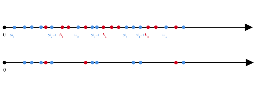
Figure 1. The first two steps in the construction: the $s_{i}$ points are represented in blue, while the $t_{i}$ points in red. Observe that in the second step all red points (and corresponding blue points not shown in the picture) between $s_{i_{j}-1}$ and $s_{i_{j}}$ are removed, so that in future steps new intervals are picked.

5.3. Proof of Theorem 1.1.

By Theorem 4.2, we already know that $\limsup_{\alpha\to\infty}\alpha^{4}\sigma^{2}(\alpha)\leq K$. Now, by definition of $C_{5}$ in (5.21), we have ${\tilde{C}}_{1}C_{5}(C)=C_{4}(C)-\frac{{\tilde{C}}_{1}{\tilde{C}}_{3}}{C}$, and by (5.14), $\lim_{C\uparrow\infty}C_{4}(C)=[{\rm e}^{-1}-{\rm e}^{-2}]\int_{\mathbb{R}^{3}}|\psi_{0}(x)|^{2}{\rm d}x$, while $\frac{{\tilde{C}}_{1}{\tilde{C}}_{3}}{C}\downarrow 0$ as $C\uparrow\infty$. Hence, there is $C_{*}\in(0,\infty)$ such that for all $\alpha>0$,

$$\alpha^{4}\sigma^{2}(\alpha)\leq\frac{1}{C_{*}\int_{\mathbb{R}^{3}}|\psi_{0}(x)|^{2}{\rm d}x},\qquad\mbox{or}\qquad\frac{m(\alpha)}{\alpha^{4}}\geq C_{*}\int_{\mathbb{R}^{3}}|\nabla\psi_{0}(x)|^{2}{\rm d}x,$$

proving Theorem 1.1. ∎

Acknowledgement: The first two authors are supported by the Deutsche Forschungsgemeinschaft (DFG) under Germany’s Excellence Strategy EXC 2044 - 390685587, Mathematics Münster: Dynamics - Geometry - Structure.

References

- [1] F. Baccelli and P. Brémaud Elements of queueing theory Springer-Verlag, Berlin (2003).
- [2] V. Betz and S. Polzer. A functional central limit theorem for polaron path measures. Comm. Pure Appl. Math. 75, 2345-2392 (2022)
- [3] V. Betz and S. Polzer. Effective mass of the Polaron: a lower bound. Comm. Math. Phys. 399, 173-188 (2023)
- [4] E. Bolthausen, W. König and C. Mukherjee. Mean field interaction of Brownian occupation measures, II.: Rigorous construction of the Pekar process. Comm. Pure Appl. Math., 70 1598-1629, (2017)
- [5] M. Brooks and R. Seiringer. The Frölich Polaron at Strong Coupling-Part II: Energy-Momentum Relation and Effective Mass. arXiv: 2211.03353 (2022)
- [6] D.J. Daley and D. Vere-Jones An introduction to the theory of point processes. Vol. I. Elementary Theory and Methods. Springer (2003).
- [7] D.J. Daley and D. Vere-Jones An introduction to the theory of point processes. Vol. II. General theory and structure. Springer (2008).
- [8] M. D. Donsker and S. R S. Varadhan. Asymptotic evaluation of certain Markov process expectations for large time, IV Comm. Pure Appl. Math. 36 (1983), 183-212.
- [9] M. Donsker and S. R. S. Varadhan. Asymptotics for the Polaron. Comm. Pure Appl. Math. 505-528 (1983).
- [10] W. Dybalski and H. Spohn. Effective Mass of the Polaron-Revisited. Annales Henri Poincaré 21, 1573- 1594 (2020).
- [11] R. Feynman. Statistical Mechanics, Benjamin, Reading (1972).
- [12] W. König and C. Mukherjee. Mean-field interaction of Brownian occupation measures. I: Uniform tube property of the Coulomb functional. Ann. Inst. H. Poincaré Probab. Statist, 53, 2214-2228, (2017), arXiv: 1509.06672
- [13] L. D. Landau and S. I. Pekar. Effective mass of a polaron. Zh.Eksp.Teor.Fiz. 18, 419- 423 (1948)
- [14] E. H. Lieb. Existence and uniqueness of the minimizing solution of Choquard’s nonlinear equation. Studies in Appl. Math. 57, 93-105 (1976).
- [15] E. H. Lieb and R. Seiringer Equivalence of Two Definitions of the Effective Mass of a Polaron, J. Stat. Phys. 154, Issue 1-2, 51-57 (2014).
- [16] E. H. Lieb and R. Seiringer Divergence of the Effective Mass of a Polaron in the Strong Coupling Limit, J. Stat. Phys. 180, 23-33 (2020)
- [17] E. H. Lieb and L. Thomas. Exact ground state energy of the strong-coupling Polaron. Comm. Math. Phys., 183, (1997), 511-519.
- [18] C. Mukherjee and S. R. S. Varadhan. Brownian occupations measures, compactness and large deviations. Ann. Probab., 44 3934-3964, (2016)
- [19] C. Mukherjee and S. R. S. Varadhan. Identification of the Polaron measure I: fixed coupling regime and the central limit theorem for large times. Commun. Pure Appl. Math. 73, no. 3, 350-383 (2020). arXiv:1802.05696
- [20] C. Mukherjee and S. R. S. Varadhan. Identification of the Polaron measure in strong coupling and the Pekar variational formula. Ann. Probab. 48, 5, 2119-2144 (2020). arXiv:1812.06927
- [21] C. Mukherjee and S. R. S. Varadhan. Corrigendum and Addendum: Identification of the Polaron measure I: fixed coupling regime and the central limit theorem for large times. Commun. Pure Appl. Math. 75, no. 7, 1642-1653 (2022). (Proof of Theorem 4.5 in arXiv:1802.05696)
- [22] S. I. Pekar. Theory of polarons, Zh. Eksperim. i Teor. Fiz. 19, (1949).
- [23] M. Sellke. Almost Quartic Lower Bound for the Fröhlich Polaron’s Effective Mass via Gaussian Domination Preprint, arXiv: 2212.14023, December 2022
- [24] H. Spohn. Effective mass of the polaron: A functional integral approach. Ann. Phys. 175, (1987), 278-318.