Kinematic power corrections in TMD factorization theorem

Abstract

This work is dedicated to the study of power expansion in the transverse momentum dependent (TMD) factorization theorem. Each genuine term in this expansion gives rise to a series of kinematic power corrections (KPCs). All terms of this series exhibit the same properties as the leading term and share the same nonperturbative content. Among various power corrections, KPCs are especially important since they restore charge conservation and frame invariance, which are violated at a fixed power order. I derive and sum a series of KPCs associated with the leading-power term of the TMD factorization theorem. The resulting expression resembles a hadronic tensor computed with free massless quarks while still satisfying a proven factorization statement. Additionally, I provide an explicit check of this novel form of factorization theorem at the next-to-leading order (NLO) and demonstrate the restoration of the frame-invariant argument of the leading-power coefficient function. Numerical estimations show that incorporating the summed KPCs into the cross-section leads to an almost constant shift, which may help to explain the observed challenges in the TMD phenomenology.

1 Introduction

The transverse momentum dependent (TMD) factorization theorem is known to be an invaluable tool in understanding the transverse momentum distribution of inclusive and semi-inclusive processes across a wide range of energy regimes. The transverse momentum distribution of Z-boson or Higgs bosons, semi-inclusive deep-inelastic scattering (SIDIS), single- and double-spin asymmetries – these are only a few examples of successes of TMD factorization approach (for review see Angeles-Martinez:2015sea ; Boussarie:2023izj ). As the list of accomplished applications continues to expand, it becomes evident that the current form of TMD factorization has practical limitations. It can only be confidently applied within a restricted phase-space, which leads to many problems and tensions already today (see f.i. discussions in Vladimirov:2019bfa ; Bury:2021sue ; Bacchetta:2022awv ), and will be critical for the future generation of colliders AbdulKhalek:2021gbh ; Accardi:2023chb . Therefore, a systematic extension and refinement of the TMD factorization approach are crucial priorities for modern studies.

A principal feature of the TMD factorization approach is its ability to systematically account for the transverse momenta of partons within the hadron. As a result, the main application domain is processes characterized by transverse momenta compatible with typical hadronic scales. At the same time, the characteristic longitudinal momenta must be large enough to justify the application of the parton model. In this study, I focus on the Drell-Yan reaction ($h_{1}+h_{2}\to\gamma^{*}+X$), which is the classical case of the TMD factorization Collins:1984kg . In this particular reaction, the relevant momenta are the transverse ($q_{T}$) and longitudinal ($q^{\pm}$) components of the produced-photon momentum.

The leading term of the TMD factorization theorem is derived Collins:2011zzd ; Becher:2010tm ; Echevarria:2011epo in the limit of the longitudinal momenta being greater than any other scales. In the position-space representation, the leading term has the general form (omitting the scaling arguments for brevity)

$$\frac{d\sigma}{dq_{T}}\sim\sigma_{0}\int_{-\infty}^{\infty}\frac{d^{2}b}{(2\pi)^{2}}e^{i(bq_{T})}~{}C_{0}~{}\widetilde{F}_{1}(x_{1},b)\widetilde{F}_{2}(x_{2},b),$$ (1)

where $\widetilde{F}_{1,2}$ are TMD parton distribution functions (TMDPDFs) in the Drell-Yan case, $x_{1,2}$ are the longitudinal momentum fractions of partons. $C_{0}$ is the hard coefficient function which depends on $q^{+}q^{-}/\mu^{2}$ with $\mu$ being the factorization scale. TMD distributions satisfy the pair of evolution equations Aybat:2011zv ; Chiu:2012ir ; Scimemi:2018xaf , which have multiplicative kernels in the position space. Due to it, the position-space representation (1) is convenient in practice. The momentum-space representation of (1) is

$$\frac{d\sigma}{dq_{T}}\sim\sigma_{0}\int_{-\infty}^{\infty}d^{2}k_{1T}d^{2}k_{2T}~{}C_{0}~{}\delta^{(2)}(q_{T}-k_{1T}-k_{2T})F_{1}(x_{1},k_{1T})F_{2}(x_{2},k_{2T}),$$ (2)

where $F_{1,2}$ are TMDPDFs in the momentum space obtained by the Fourier transform of $\widetilde{F}_{1,2}$. Explicit examples of these structures for various processes can be found in refs.Mulders:1995dh ; Bacchetta:2006tn ; Arnold:2008kf . The perturbative elements of the factorization formula (1) (the hard coefficient function and the evolution kernels) are known up to next-to-next-to-next-to-next-to-leading order (N⁴LO), making it one of the most developed formula in the perturbation theory.

The corrections to the leading term are suppressed by powers of $q^{\pm}$. To simplify the exposition, I generally refer to the large scale as $Q$ ($\sim q^{+}\sim q^{-}$). The power corrections can be categorized into four conceptual types:

$k_{T}/Q$ power corrections: In the position-space representation, these corrections manifest as transverse derivatives of TMD distributions, while in the momentum representation, as the powers of $k_{T}$’s. These corrections are commonly known as kinematic power corrections (KPCs).

$q_{T}/Q$ power corrections: In the position space, these corrections arise as terms accompanied by inverse powers of $b$. Once integrated, such factors transform into powers of $q_{T}$.

$\Lambda/Q$ power corrections: These corrections indicate terms that contain nonperturbative distributions of higher twist. Generally, a TMD distribution of twist-n is considered as a $(\Lambda/Q)^{n-2}$ correction. These corrections are often referred to as higher twist power corrections.

Target-mass corrections: These corrections account for the finite mass of the hadron. Currently, they are the least studied corrections.

Let me emphasize the difference between $k_{T}/Q$ and $q_{T}/Q$ power corrections since they were not distinguished until recently. Indeed, in the momentum-space representation (2), these corrections can be confused with each other due to the relation $q_{T}=k_{1T}+k_{2T}$. Nonetheless, they have conceptually different origins. The $q_{T}/Q$-corrections are related to the common ultra-violet (UV) singular behavior at $b\to 0$ and are merely a part of the hard scattering sub-process. The $k_{T}/Q$-corrections are UV-finite and are a part of low-energy dynamics. In the position space, the $k_{T}/Q$-corrections appear as the transverse derivatives of $\tilde{F}(x,b)$’s that turn to parton’s $k_{T}$’s in the momentum space representation, which suggests the name. Therefore, these corrections are entirely independent from the theory point of view. Practically, these power corrections are also distinct. KPCs are non-vanishing in the limit $q_{T}\to 0$ (the traditional TMD limit) and remain of the same order for larger $q_{T}$. On the contrary, the $q_{T}/Q$-corrections vanish at $q_{T}\to 0$ and grow at larger $q_{T}$ (as suggested by name), and constitute the major part of the famous Y-term Collins:1984kg ; Collins:2011zzd ; Boussarie:2023izj . Below, I present more details on their definition.

Together, four types of power corrections form a complex system, which is discussed further in the remaining part of the introduction. Importantly, each type of power correction exhibits distinct theoretical and practical features, making some corrections more significant than others in different circumstances. In this study, I present the derivation, summation, and discussion of (pure) KPCs and examine their practical importance.

In recent years, there has been significant progress in the study of power corrections to the TMD factorization theorem Balitsky:2017gis ; Balitsky:2020jzt ; Inglis-Whalen:2021bea ; Balitsky:2021fer ; Vladimirov:2021hdn ; Ebert:2021jhy ; Rodini:2022wic ; Rodini:2023plb . This progress has been made possible by formulating the TMD factorization on the operator level, as opposed to the method-of-region analysis Collins:2011zzd used in the original derivation of the leading power (LP) term. As a matter of fact, the power corrections are simpler to analyze with operator methods since they allow for unambiguous identification of the different types of power corrections. This is crucial for a comprehensive understanding of the structure of the factorization theorem beyond the LP approximation. Still, the status of the TMD factorization theorem beyond the LP approximation remains an open problem. Currently, there exists a complete expression for TMD factorization at the next-to-leading power (NLP) level. It has been derived with three different methods Balitsky:2021fer ; Vladimirov:2021hdn ; Ebert:2021jhy (and agrees between them), and checked at next-to-leading order (NLO) Vladimirov:2021hdn ; Rodini:2022wic ; Rodini:2022wki . Furthermore, several general statements (such as the all-order structure of rapidity divergences for twist-three distributions Vladimirov:2021hdn ; Ebert:2021jhy , the cancellation of special rapidity divergences Rodini:2022wic ; Rodini:2022wki ) provide us hope that the NLP TMD factorization is valid at all perturbative orders. The research on the next-to-next-to-leading power (NNLP) TMD factorization is very limited Balitsky:2020jzt ; Inglis-Whalen:2021bea ; Balitsky:2021fer .

The straight evaluation of power corrections is impractical. Already at NNLP, one faces many novel theoretical problems and a vast number of structures. Therefore, to proceed further, it is crucial to understand and account for the general hierarchy of power-suppressed terms in the TMD factorization framework. This hierarchy can be deduced from the power counting and the dimension analysis. Naturally, there is a degree of arbitrariness in such a generalization. Nonetheless, if TMD factorization holds at higher powers, one should expect it to exhibit the following general structure (omitting target-mass corrections for simplicity)

$$W^{\mu\nu}=\frac{1}{N_{c}}\int\frac{d^{2}b}{(2\pi)^{2}}\,e^{-i(q_{T}b)}\Bigg{\{}$$ (3)

$$\phantom{+\frac{1}{Q\phantom{{}^{1}}}\Big{(}D^{0}}\Phi_{\mathbf{2}}\times\Phi_{\mathbf{2}}$$

$$+\frac{1}{Q\phantom{{}^{1}}}\Big{(}D\phantom{{}^{1}}\Phi_{\mathbf{2}}\times\Phi_{\mathbf{2}}+\phantom{D^{0}}\Phi_{\mathbf{2}}\times\Phi_{\mathbf{3}}\Big{)}$$

$$+\frac{1}{Q^{2}}\Big{(}D^{2}\Phi_{\mathbf{2}}\times\Phi_{\mathbf{2}}+D\phantom{{}^{1}}\Phi_{\mathbf{2}}\times\Phi_{\mathbf{3}}+\phantom{D}\Phi_{\mathbf{3}}\times\Phi_{\mathbf{3}}+\phantom{D}\Phi_{\mathbf{2}}\times\Phi_{\mathbf{4}}+\frac{\Phi_{\mathbf{2}}\times\Phi_{\mathbf{2}}}{b^{2}}\Big{)}$$

$$+\frac{1}{Q^{3}}\Big{(}D^{3}\Phi_{\mathbf{2}}\times\Phi_{\mathbf{2}}+D^{2}\Phi_{\mathbf{2}}\times\Phi_{\mathbf{3}}+D\Phi_{\mathbf{3}}\times\Phi_{\mathbf{3}}+D\Phi_{\mathbf{2}}\times\Phi_{\mathbf{4}}+\frac{D\Phi_{\mathbf{2}}\times\Phi_{\mathbf{2}}}{b^{2}}+\Phi_{\mathbf{3}}\times\Phi_{\mathbf{4}}+...\Big{)}$$

$$+\cdots\Bigg{\}}^{\mu\nu},$$

where $\Phi_{\mathbf{n}}$ is a TMD distribution of twist-n, which depends on $b$ and some number of collinear-momentum fractions. The power of $D$ indicates the number of boost-invariant transverse derivatives (defined in (69)) in the term, which acts to TMD distributions in various combinations. The symbol $\times$ indicates an integral convolution in the collinear-momentum fractions. Each term is equipped with a coefficient function which is not shown. The first line in the brackets is the LP term (1). The second line is the NLP term (see Balitsky:2020jzt ; Vladimirov:2021hdn ), and so on. Each term in expression (3) represents a complicated composition of various distributions.

In expression (3), one can easily recognize power corrections of different types. So, the first term in the third line ($D\Phi_{\mathbf{2}}\times\Phi_{\mathbf{2}}$) is the correction $\sim k_{T}/Q$, and the second term ($\Phi_{\mathbf{2}}\times\Phi_{\mathbf{3}}$) is the correction $\Lambda/Q$. In the fourth line, the first term ($D^{2}\Phi_{\mathbf{2}}\times\Phi_{\mathbf{2}}$) is $k_{T}^{2}/Q^{2}$, the second term ($D\Phi_{\mathbf{2}}\times\Phi_{\mathbf{3}}$) is $k_{T}\Lambda/Q^{2}$, the third and forth terms ($\Phi_{\mathbf{3}}\times\Phi_{\mathbf{3}}$ and $\Phi_{\mathbf{2}}\times\Phi_{\mathbf{4}}$) are $\Lambda^{2}/Q^{2}$, and the last term ($\Phi_{\mathbf{2}}\times\Phi_{\mathbf{2}}/b^{2}$) is $q_{T}^{2}/Q^{2}$. And so on.

In eqn. (3), the terms with different order of $k_{T}/Q$ corrections but the same order of other corrections are aligned into columns. These columns represent a series of KPCs to the first term. Each column incorporates unique nonperturbative content, as it contains a combination of TMD distributions that do not appear in other columns. Hence, each column can be considered as an independent contribution to the TMD factorization theorem. All global properties expected from the hadronic tensor, such as charge conservation and frame invariance, must hold for each column individually.

It is important to emphasize that the decomposition (3) is based on the assumption that TMD distributions of different twists (i.e., $\Phi_{\mathbf{n}}$ and $\Phi_{\mathbf{m}}$ for $n\neq m$) are completely independent functions. This assumption holds if these distributions do not mix under TMD evolution. The requirement for non-mixture is a fundamental prerequisite because otherwise, power corrections of different types would entangle due to evolution or by higher perturbative orders of coefficient functions, and the presentation form (3) would be impossible. Moreover, it would violate the universality property of nonperturbative distributions. Therefore, the problem of systematization of power corrections in TMD factorization is equivalent to the problem of the definition of TMD-twist. This work adopts the definition of TMD twist introduced in ref. Vladimirov:2021hdn , which constitutes a TMD generalization of the concept of geometrical twist (aka ”dimension minus spin”) used for collinear operators Brandt:1970kg ; Gross:1971wn . This definition ensures, at least, the independence of non-mixture under ultraviolet renormalization.

Apart from the theoretical challenges posed by power-suppressed terms, there is also a practical concern regarding their relevance. It is evident that a plethora of TMD distributions appear in the power corrections, and the number of new functions grows faster than the number of observables. Already at NLP, one encounters 32 twist-three TMDPDFs Rodini:2022wki (in addition to the 8 TMDPDFs at the leading power). Identifying and constraining all these functions from experimental data alone is practically impossible. In this regard, higher twist power corrections can be characterized as ”bad” as they introduce unknown functions (although offering insights into new facets of quantum physics). The other types of power corrections are ”better” as they do not increase the number of unknowns but instead refine and extend the LP term.

Thus, it is sensible to incorporate power corrections by types rather than by orders. First, this approach preserves the validity of the factorization theorem, as different types of power corrections are additive and do not interfere with each other. Secondly, each type of correction contributes to a specific kinematic region and could be distinguished phenomenologically. Neglecting power corrections put the requirements to the applicability range of the factorization theorem. Each power correction leads to its own limitation, and therefore, the LP TMD factorization is valid in the regime

$$k_{T}\ll Q,\quad q_{T}\ll Q,\quad\Lambda\ll Q,\quad m\ll Q.$$ (4)

Including power corrections of a specific type softens the corresponding restriction, while summing the power corrections of a specific type eliminates the restriction (or replaces it with a strict inequality). At low $Q$, all types of power corrections are significant simultaneously. Notably, the $q_{T}/Q$ corrections are special, as their magnitude is controlled by the experimental kinematics. By including only $q_{T}/Q$ corrections, the cross-section can be described up to $q_{T}\sim Q$, while the other corrections remain negligible (for large $Q$). The remaining corrections follow a hierarchy of $k_{T}>m>\Lambda$ and are valid in the regime $q_{T}\ll Q$.

In this work, I study KPCs for the LP term. Within the expression (3), these power corrections are represented by the first column. Notably, these power corrections are of utmost importance within the conventional range of application for TMD factorization $q_{T}\ll Q$. Primarily, KPCs play a crucial role in restoring the electromagnetic (EM) gauge invariance (charge conservation) and frame invariance of the hadronic tensor, both of which are explicitly broken in the LP term. Consequently, KPCs can be viewed as an integral part of the LP factorization, as the absence of these corrections render the LP factorization inconsistent. Furthermore, unlike other scales such as $q_{T}$, $\Lambda$, or $m$, the scale $k_{T}$ is not fixed but rather an integration variable (2). This introduces a self-contradiction, as the factorization formula includes values of $k_{T}$ that exceed $Q$, contradicting the initial assumption that $Q$ is the largest scale. Moreover, the average value of $k_{T}$ is of the order of the ultraviolet cut-off due to the large-$k_{T}$ asymptotic behavior of TMD distributions ($\sim k_{T}^{-2}$). An extra point in favor of KPCs is that the factorization theorem for them does not require a dedicated proof. KPCs inherit the factorization property from the LP term, for which the theorem is already proven. Considering these reasons, it is sufficient to include KPCs independently of other power corrections.

The paper is structured as follows. In sec. 2 I review the concept of the TMD-twist and present in detail the simplest (but the most useful) example of twist-decomposition for the quark operator (sec. 2.2) and for a general bi-quark TMD distribution (sec. 2.3). Sec. 3 is dedicated to the derivation of KPCs order-by-order in power expansion. Here, I start from the sketch of the operator derivation of the LP term (sec. 3.1) and continue to this derivation to all-powers (sec. 3.2). In sec. 3, I inspect the influence of loop corrections for KPCs and derive the argument of the coefficient function. The summation of the KPC series is done in sec. 4. To perform the summation, I first sum the series of twist-two terms for a general TMD correlator (sec. 4.1) and then insert it into the factorized expression (sec. 4.2). In sec. 5, I inspect the properties of the summed expression, using the example of a completely unpolarized contribution to hadron tensor of Drell-Yan. The subsections 5.1 and 5.2 are devoted to the EM gauge invariance and the frame invariance, correspondingly. Finally, the estimation of numerical impact is presented in sec. 5.3.

2 Twist decomposition in TMD factorization

The definition of TMD-twist is vital for systematisation of power corrections. Given this definition, it becomes possible to decompose operators of any dimension into irreducible components and express their matrix elements in terms of universal and independent nonperturbative TMD distributions. A suitable definition of TMD-twist was proposed in reference Vladimirov:2021hdn . TMD-twist is determined by a pair of geometrical twists associated with the semi-compact operators that constitute any TMD operator. This approach strictly ensures non-mixture of operators with distinct TMD-twists under evolution with the ultraviolet (UV) renormalization scale $\mu$. Although the non-mixture under the rapidity evolution remains questionable, this property has been demonstrated in Vladimirov:2021hdn for a wide range of TMD distributions (given by quasi-partonic operators), which encompasses all TMD distributions of twist-two and twist-three. Furthermore, the equivalence of rapidity evolution between TMD distributions of TMD-twist two and three was established in Ebert:2021jhy . Therefore, this definition is satisfactory for the current objective, namely the determination of KPCs for the LP term, as they solely include TMD distributions of twist-two.

In this section, I provide a review of the general definition of TMD-twist and present the simplest yet non-trivial example of twist-decomposition. This example serves as the foundation for the subsequent computation of KPCs.

2.1 TMD-twist

At any power of TMD factorization theorem TMD distributions have the same general structure,

$$\widetilde{\Phi}_{AB}(\{z\}_{A},\{z\}_{B};b)\sim\langle p,s|U_{A}(\{z\}_{A};b)U_{B}(\{z\}_{B};0)|p,s\rangle,$$ (5)

where $U$ is a light-cone operator, labels $A$ and $B$ indicate the quantum numbers of $U$, and $\{z\}_{A}$ is a set of coordinates $z$. The operator $U(\{z\}_{A};b)$ is a T-ordered product of QCD fields positioned at $(z_{i}n+b)$ for $z_{i}\in\{z\}_{A}$. The fields in the operator are connected by light-like Wilson lines, which continue to the light-cone infinity. So, the operator $U$ spans an infinite range, and for that reason it is called semi-compact.

The renormalization of TMD distribution consists of two renormalization factors – one for each operator $U$. These factors are independent since the distance between operators is transverse and thus UV finite. The evolution equation reads

$$\mu^{2}\frac{d}{d\mu^{2}}\widetilde{\Phi}_{AB}(\{z\}_{A},\{z\}_{B};b)=\left(\tilde{\gamma}_{A}(\{z\}_{A})+\tilde{\gamma}_{B}(\{z\}_{B})\right)\otimes\widetilde{\Phi}_{AB}(\{z\}_{A},\{z\}_{B};b),$$ (6)

where $\tilde{\gamma}_{A}$ is the anomalous dimension of $U_{A}$ and $\otimes$ is the integral convolution in corresponding positions $\{z_{i}\}$. Note, that anomalous dimensions $\tilde{\gamma}$ contain the double logarithmic part, which is resulted from gluon propagated along Wilson line to the infinity (collinear singularity). The same singularity is presented in the rapidity renormalization factor (or soft factor). Their cancellation leads to a logarithm contribution $\sim\ln(\mu^{2}/\zeta)$ in the anomalous dimensions.

The equation (6) describes only the UV evolution, while TMD distributions also obey rapidity evolution equation (30). Currently, there is no general consensus regarding the rapidity divergences of operators that arise at higher powers. The only established result is that all quasi-partonic TMD operators conform to the leading power (LP) rapidity evolution Vladimirov:2021hdn . Thus, it is plausible that the present definition of TMD-twist is incomplete, and some operators could potentially mix due to the rapidity evolution. However, this hypothetical situation would only apply to non-quasi-partonic TMD distributions, which have a minimum twist-four and emerge at NNLP for the first time, and thus, are irrelevant for the present discussion.

The light-cone operators $U_{A}$ and $U_{B}$ have independent anomalous dimensions if they have different geometrical twist (defined as “dimension-minus-spin” of the operator). Consequently, TMD distributions $\widetilde{\Phi}_{AB}$ and $\widetilde{\Phi}_{A^{\prime}B^{\prime}}$ do not mix with each other if the geometrical twist of $U_{A}$ or $U_{B}$ is different from the geometrical twist of $U_{A^{\prime}}$ or $U_{B^{\prime}}$. It gives raise to a natural definition of TMD-twist for $\widetilde{\Phi}_{AB}$, as a pair of integer numbers $(N,M)$, where $N$($M$) is a geometrical twist of semi-compact operator $U_{A(B)}$.

Formally, the definition of geometrical twist is defined only for local operators. Its generalization for semi-compact operator can be done by the following procedure. First, one selects $L$ such that $\{|z|\}<|L|$, and drop the part of Wilson line from $Ln$ to infinity. Next, the operator is expanded as series at $L$. It takes a form $U_{A}(z,0)\sim\sum_{n}(z-L)^{n}U_{A,n}$, where $U_{A,n}$ are local operators. The geometric twist of local operators $U_{A,n}$ is the geometric twist of semi-compact operator $U_{A}$. After the decomposition of operator into components with the same twist, each component can be summed over $n$. Finally, the limit $L\to\infty$ is taken. This method properly reconstructs the properties of semi-compact operators, as it is demonstrated in ref. Moos:2020wvd .

An indication of twist for TMD operator by a single number (used so far), refers to $(N+M)$. For example, it was used in the expression (3), where $\Phi_{\mathbf{n}}=\Phi_{MN}$ with $N+M=n$. Meanwhile, all TMD distributions of twist-two have TMD-twist $(1,1)$. However, the single-number terminology is ambiguous beyond the twist-two case. For example, a TMD distribution of twist-three can have TMD-twist $(1,2)$ or $(2,1)$, which are two entirely independent distributions with separate evolution equations (see ref.Rodini:2022wki ). TMD distribution of twist-four can have TMD-twist $(1,3)$, $(3,1)$ or $(2,2)$, and so on. Still, the single-number indication is shorter and it is convenient to use if it does not create a confusion.

2.2 Example of twist-decomposition

As an example of twist decomposition let me consider the simplest semi-compact operator that appears in the TMD factorization. It is a quark field with an attached semi-infinite Wilson line

$$U_{q}(0,0_{T})=[-\infty n,0]q(0).$$ (7)

where $[an,bn]$ is a Wilson line along $n$

$$[an,bn]=P\exp\left(-ig\int_{a}^{b}dsA_{+}(sn)\right).$$ (8)

As usually, the vectors $n^{\mu}$ and $\bar{n}^{\mu}$ are two independent light-cone vectors with normalization

$$n^{2}=\bar{n}^{2}=0,\qquad(n\bar{n})=1.$$ (9)

The decomposition of any vector $v^{\mu}$ reads

$$v^{\mu}=\bar{n}^{\mu}v^{+}+n^{\mu}v^{-}+v_{T}^{\mu},$$ (10)

where $v^{+}=(nv)$, $v^{-}=(\bar{n}v)$ and $v_{T}$ is the transverse component orthogonal to $(n,\bar{n})$-plane $v_{T}^{\mu}=g_{T}^{\mu\nu}v_{\nu}$ with

$$g_{T}^{\mu\nu}=g^{\mu\nu}-n^{\mu}\bar{n}^{\nu}-\bar{n}^{\mu}n^{\nu}.$$ (11)

Following the procedure described above the operator (7) can be presented as

$$U_{q}(0,0_{T})=\lim_{L\to-\infty}\sum_{n=0}^{\infty}\frac{i^{n}L^{n}}{n!}D_{+}^{n}q(Ln),$$ (12)

where $D_{\mu}=\partial_{\mu}-igA_{\mu}$ is the QCD covariant derivative. The local operator $D_{\mu_{1}}...D_{\mu_{n}}q_{i}$ has the mass-dimension $n+3/2$. It is a Lorenz tensor of mixed nature with $n$ vector indices and one spinor index. The maximum possible spin of this tensor is $n+1/2$. To achieve it, one should symmetrize indices $\mu$, subtract traces (in the present case, it automatically achieved by contraction with $n^{\mu_{1}}...n^{\mu_{n}}$), and make the spinor index $\gamma$-traceless Rarita:1941mf , i.e. such that $\gamma^{\mu_{j}}D_{\mu_{1}}...D_{\mu_{j}}...D_{\mu_{n}}q=0$ (for a more formal discussion see refs.DelgadoAcosta:2015ypa ; Geyer:1999uq ). For the present tensor (that is contracted with $n^{\mu_{1}}...n^{\mu_{n}}$) it implies that the maximum-spin operator should vanish after multiplication by $\gamma^{-}$. It leads to a natural decomposition of the spinor into “good” and “bad” components Jaffe:1991kp , as $q=\xi_{\bar{n}}+\eta_{\bar{n}}$, where

$$\xi_{\bar{n}}=\frac{\gamma^{-}\gamma^{+}}{2}q,\qquad\eta_{\bar{n}}=\frac{\gamma^{+}\gamma^{-}}{2}q.$$ (13)

Here, the subscript $\bar{n}$ indicates that these components are defined with respect to $\gamma^{-}$. Since $\gamma^{-}\xi=0$, the operator $D_{+}^{n}\xi$ has the maximum spin, and its geometrical twist equals one. Summing the series over $n$ and limiting $L\to-\infty$, the twist-one part of (7) is

$$U_{q}(0,0_{T})\Big{|}_{\text{tw-1}}=U_{1}(0,0_{T})=[-\infty n,0]\xi_{\bar{n}}(0).$$ (14)

The remaining part of $U_{q}$ is $[-\infty n,0]\eta_{\bar{n}}(0)$. It is twist-two, but the field $\eta$ is not dynamically independent. The components $\eta$ and $\xi$ are related to each other via the QCD equation of motion (EOM). The EOM is $\not{D}q=0$ for massless quark. After projection (13) EOM splits into two equations, which are convenient to write as

$$D_{+}\eta_{\bar{n}}=-\frac{1}{2}\gamma^{+}\not{D}_{T}\xi_{\bar{n}},\qquad D_{-}\xi_{\bar{n}}=-\frac{1}{2}\gamma^{-}\not{D}_{T}\eta_{\bar{n}}.$$ (15)

Inserting the left equation into eqn. (12) and commuting the transverse derivative to the outer position one gets

$$D_{+}^{n}\eta_{\bar{n}}(Ln) = \frac{-1}{2}\gamma^{+}\gamma^{\mu}_{T}D_{+}^{n-1}D_{\mu}\xi_{\bar{n}}(Ln)$$

$$= \frac{-1}{2}\gamma^{+}\gamma^{\mu}_{T}\left(D_{\mu}D_{+}^{n-1}\xi_{\bar{n}}(Ln)+ig\sum_{m=0}^{n-1}D_{+}^{n-m}F_{\mu+}D_{+}^{m}\xi_{\bar{n}}(Ln)\right),$$

where $F_{\mu\nu}=ig^{-1}[D_{\mu},D_{\nu}]$ is the gluon field-strength tensor. The subscript on a gamma-matrix indicates that its index is transverse. The summing over $n$ gives

$$[Ln,0]\eta_{\bar{n}}(0) = \frac{-1}{2}\gamma^{+}\gamma^{\mu}_{T}\int_{-\infty}^{0}ds\Big{(}D_{\mu}[Ln,sn]\xi_{\bar{n}}(sn)+ig\int_{L}^{s}ds_{1}[Ln,s_{1}n]F_{\mu+}[s_{1}n,sn]\xi_{\bar{n}}(sn)\Big{)}.$$ (17)

The spin of the last term is $n-1/2$, since it is traceless and $\gamma$-traceless, and has all, except one, indices symmetrized. Thus, the last term is twist-two operator.

The final expression for twist-decomposition of $U_{q}$ can be assembled. Let the transverse component of the gluon field vanish at light-cone infinity, so $\lim_{L\to\infty}D_{\mu}(L)=\partial_{\mu}$. Then combining (14) and (17), one receives

$$U_{q}(0,0_{T})=U_{1}(0,0_{T})-\frac{\gamma^{+}\gamma^{\mu}_{T}}{2}\int_{-\infty}^{0}ds\partial_{\mu}U_{1}(s,0_{T})-i\frac{\gamma^{+}\gamma^{\mu}_{T}}{2}\int_{-\infty}^{0}ds\int_{-\infty}^{s}ds_{1}U_{2,\mu}(s_{1},s,0_{T}),$$ (18)

where $U_{1}$ is the twist-one operator (14) and $U_{2}$ is the twist-two operator

$$U_{2,\mu}(z_{1},z_{2},0_{T})=g[-\infty n,z_{1}n]F_{\mu+}[z_{1}n,z_{2}n]\xi_{\bar{n}}(z_{2}n).$$ (19)

Therefore, the operator $U_{q}$ is decomposed into operators of twist-one (first term) and twist-two (last term), and the total derivative of twist-one operator (second term). The procedure presented above is standard for analysis of higher-twist collinear operators, see e.g. examples in refs. Jaffe:1996zw ; Balitsky:1987bk ; Belitsky:2000vx . The only difference in the present case is the open spinor index, which should be extra treated in the tensor decomposition.

Note that the “good” and “bad” components has also different counting with respect to $\lambda\sim k_{T}/k_{+}$. Assuming that a quark field has large $k^{+}$ and almost massless $k^{2}\sim 0$, one finds that $\eta_{\bar{n}}\sim\lambda\xi_{\bar{n}}$ from EOMs (15). This counting is convenient to use for sorting operators in the power series, and it is widely used.

2.3 Twist-decomposition for bi-quark TMD distribution

The procedure of twist-decomposition for semi-compact operators leads to the decomposition of TMD matrix elements to definite twist parts. Let me demonstrate it for the bi-quark TMD matrix element, which is also important for derivation of KPCs. The matrix element reads

$$\widetilde{\Phi}_{\bar{q}q}^{[\gamma^{\mu}]}(x,b) = \int_{-\infty}^{\infty}\frac{dz}{2\pi}e^{-ixzp^{+}}\langle p|\overline{U}_{q}(zn,b)\frac{\gamma^{\mu}}{2}U_{q}(0,0_{T})|p\rangle,$$

$$= \int_{-\infty}^{\infty}\frac{dz}{2\pi}e^{-ixzp^{+}}\langle p|\bar{q}(zn+b)[zn+b,-\infty n+b]\frac{\gamma^{\mu}}{2}[-\infty n,0]q(0)|p\rangle,$$

where $|p\rangle$ is a hadron state with momentum $p$, $b$ is a transverse vector and $\overline{U}=U^{\dagger}\gamma^{0}$. Being contracted with $n^{\mu}$ this matrix element results into the unpolarized and Sivers TMD distributions that are twist-two TMD distribution. For a general $\gamma^{\mu}$, the matrix element $\widetilde{\Phi}_{\bar{q}q}^{[\gamma^{\mu}]}$ does not represent a conventional distribution, but is a sum of distributions with different properties. It can be checked by computing the renormalization of matrix element (2.3) and observing that it could not be expressed via $\widetilde{\Phi}^{[\gamma^{\mu}]}$ (see f.i. computations in refs.Rodini:2022wki ; Gamberg:2022lju ). The reason is that the operator (2.3) has an undefinite twist.

Inserting the decomposition (18) into (2.3), the correlator $\widetilde{\Phi}^{[\gamma^{\mu}]}_{\bar{q}q}$ turns into

$$\widetilde{\Phi}_{\bar{q}q}^{[\gamma^{\mu}]}(x,b)=\int_{-\infty}^{\infty}\frac{dz}{2\pi}e^{-ixzp^{+}}\Bigg{[}\langle p|\overline{U}_{1}(z,b)\frac{\gamma^{\mu}}{2}U_{1}(0,0_{T})|p\rangle$$ (21)

$$\quad-\frac{1}{2}\int_{-\infty}^{0}ds\Big{\langle}p\Big{|}\overline{U}_{1}(z,b)\frac{\gamma^{\mu}\gamma^{+}\gamma^{\nu}_{T}}{2}\overrightarrow{\partial}_{\nu}U_{1}(s,0_{T})+\overline{U}_{1}(z+s,b)\overleftarrow{\partial}_{\nu}\frac{\gamma_{T}^{\nu}\gamma^{+}\gamma^{\mu}}{2}U_{1}(0,0_{T})\Big{|}p\Big{\rangle}$$

$$\quad+\frac{1}{4}\int_{-\infty}^{0}dsdt\langle p|\overline{U}_{1}(z+s,b)\overleftarrow{\partial}_{\nu}\frac{\gamma_{T}^{\nu}\gamma^{+}\gamma^{\mu}\gamma^{+}\gamma^{\rho}_{T}}{2}\overrightarrow{\partial}_{\rho}U_{1}(t,0_{T})|p\rangle$$

$$\quad+\frac{i}{2}\int_{-\infty}^{0}ds\int_{-\infty}^{s}ds_{1}$$

$$\qquad\Big{\langle}p\Big{|}\overline{U}_{2,\nu}(z+s,z+s_{1},b)\frac{\gamma^{\nu}_{T}\gamma^{+}\gamma^{\mu}}{2}U_{1}(0,0_{T})-\overline{U}_{1}(z,b)\frac{\gamma^{\mu}\gamma^{+}\gamma^{\nu}_{T}}{2}U_{2,\nu}(s_{1},s,0_{T})\Big{|}p\Big{\rangle}$$

$$\quad-\frac{i}{4}\int_{-\infty}^{0}dt\int_{-\infty}^{0}ds\int_{-\infty}^{s}ds_{1}\Big{\langle}p\Big{|}\overline{U}_{2,\nu}(z+s,z+s_{1},b)\frac{\gamma^{\nu}_{T}\gamma^{+}\gamma^{\mu}\gamma^{+}\gamma_{T}^{\rho}}{2}\partial_{\rho}U_{1}(t,0_{T})$$

$$\qquad\qquad\qquad\qquad\qquad\qquad\qquad-\overline{U}_{1}(z+t,b)\overline{\partial}_{\rho}\frac{\gamma^{\rho}_{T}\gamma^{+}\gamma^{\mu}\gamma^{+}\gamma^{\nu}_{T}}{2}U_{2,\nu}(s_{1},s,0_{T})\Big{|}p\Big{\rangle}$$

$$\quad+\frac{1}{4}\int_{-\infty}^{0}dt\int_{-\infty}^{t}dt_{1}\int_{-\infty}^{0}ds\int_{-\infty}^{s}ds_{1}\Big{\langle}p\Big{|}\overline{U}_{2,\nu}(z+s,z+s_{1},b)\frac{\gamma^{\nu}_{T}\gamma^{+}\gamma^{\mu}\gamma^{+}\gamma_{T}^{\rho}}{2}U_{2,\rho}(t,t_{1},0_{T})\Big{|}p\Big{\rangle}\Bigg{]}~{},$$

where $\overline{U}=U^{\dagger}\gamma^{0}$. The matrix element in the first three lines are the TMD distributions of TMD-twist-(1,1). The lines fifth to seventh are TMD distributions with TMD-twists-(2,1) and (1,2). The last line is the TMD distribution of TMD-twist-(2,2).

The gamma-structure of (21) can be simplified using that the spinor indices of operators $U$ projected by matrices (13). For example, one finds that $\overline{U}_{1}\gamma^{\mu}U_{1}=\bar{n}^{\mu}\overline{U}_{1}\gamma^{+}U_{1}$. The total derivatives of operators $U$ can be pushed outside of matrix elements using that

$$\langle p|\partial_{\mu}(...)|p\rangle=0.$$ (22)

After these simplifications the result reads

$$\widetilde{\Phi}^{[\gamma^{\mu}]}_{\bar{q}q}(x,b) = \left(\bar{n}^{\mu}+\frac{i}{xp^{+}}\frac{\partial}{\partial b_{\mu}}+\frac{n^{\mu}}{2(xp^{+})^{2}}\frac{\partial^{2}}{\partial b^{\nu}\partial b_{\nu}}\right)\widetilde{\Phi}^{[\gamma^{+}]}_{11}(x,b)+...~{},$$ (23)

where $\Phi^{[\gamma^{+}]}_{11}$ is a TMD distribution of TMD-twist-(1,1)

$$\widetilde{\Phi}^{[\Gamma]}_{11}(x,b) = \int_{-\infty}^{\infty}\frac{dz}{2\pi}e^{-ixzp^{+}}\langle p|\overline{U}_{1}(z,b)\frac{\Gamma}{2}U_{1}(0,0_{T})|p\rangle,$$ (24)

and dots denote contributions with TMD-twist-(1,2), (2,1) and (2,2) resulted from the last five lines of (21). The expression (23) is the twist-two part of the correlator (2.3).

The momentum space representation of TMD distribution is obtained by

$$\widetilde{\Phi}^{[\Gamma]}(x,b)=\int d^{2}k_{T}e^{i(bk_{T})}\Phi^{[\Gamma]}(x,k_{T}).$$ (25)

Here and in the following, I use the (un)tilded notation to indicate the distributions in the (momentum) position space. The momentum space representation of (23) is

$$\Phi_{\bar{q}q}^{[\gamma^{\mu}]}(x,k_{T}) = \left(\bar{n}^{\mu}+\frac{k_{T}^{\mu}}{xp^{+}}-\frac{n^{\mu}k_{T}^{2}}{2(xp^{+})^{2}}\right)\Phi^{[\gamma^{+}]}_{11}(x,k_{T})+...~{}.$$ (26)

The derivatives over $b$ turn into powers of $k_{T}$.

It is also critical to observe that total derivatives of semi-compact operators does not always result to the definite-twist TMD distributions. It works out for total derivatives $\partial_{+}$ (which produces factors of $x$ in the momentum space), and $\partial_{\mu T}$ (which produces factors of $k_{T}^{\mu}$). However, total derivatives $\partial_{-}$ cannot be moved outside of the operator. Nonetheless, they could be always expressed via $\partial_{+}$, $\partial_{\mu T}$ and extra gluon fields, thanks to EOMs (15). The example is given in sec. 3.2.

The expression (26) can be written as

$$\Phi^{[\gamma^{\mu}]}_{\bar{q}q}(x,k_{T}) = 2\int_{-\infty}^{\infty}dk^{-}\,k^{\mu}\delta(k^{2})\Phi^{[\gamma^{+}]}_{11}(x,k_{T})+...~{},$$ (27)

with $k^{\mu}=xp_{+}\bar{n}^{\mu}+k_{T}^{\mu}+n^{\mu}k^{-}$ being the four-momentum of the parton. This respresentation gives rise to an interpretation of the leading twist distributions, as the part of the hadron’s structure carried by the free-quark approximation. In the sec. 4.1 I provide a further generalization of eqn.(27).

The twist-decomposition is a standard procedure for consideration of power corrections for factorization theorems, and the expressions (18) and (23) are rather typical for such kind of calculus. Many analogies can be found in the literature related to the collinear factorization. For example, the expressions (23) and (26) are ideologically analogous to the Wandzura-Wilczek approximation for collinear distributions Wandzura:1977qf . In the present work, the main interest is the terms with total derivatives of the leading twist operator. These terms are responsible for generation of KPCs. It is analogous to the case of Deeply-Virtual Compton Scattering (DVCS) and Generalized parton distributions (GPDs) Braun:2011dg ; Braun:2011zr .

Note that for the operator with a differently oriented light-like Wilson line, the vectors $n$ and $\bar{n}$ should be swapped. For example, for decomposition for the operator $[-\infty\bar{n},0]q(0)$ is the same as (18) but with $n\leftrightarrow\bar{n}$. The “good” and “bad” components are defined as

$$\xi_{n}=\frac{\gamma^{+}\gamma^{-}}{2}q,\qquad\eta_{n}=\frac{\gamma^{-}\gamma^{+}}{2}q.$$ (28)

The direction of Wilson line (future vs. past) does not play a role in this example.

For the following discussion, it is important to specify the evolution equation for twist-two TMDPDFs. these equations are Aybat:2011zv ; Chiu:2012ir

$$\mu^{2}\frac{d}{d\mu^{2}}\widetilde{\Phi}_{11}^{[\Gamma]}(x,b;\mu,\zeta) = \left(\frac{\Gamma_{\text{cusp}}(\mu)}{2}\ln\left(\frac{\mu^{2}}{\zeta}\right)-\frac{\gamma_{V}(\mu)}{2}\right)\widetilde{\Phi}_{11}^{[\Gamma]}(x,b;\mu,\zeta),$$ (29)

$$\zeta\frac{d}{d\zeta}\widetilde{\Phi}_{11}^{[\Gamma]}(x,b;\mu,\zeta) = -\mathcal{D}(b,\mu)\widetilde{\Phi}_{11}^{[\Gamma]}(x,b;\mu,\zeta),$$ (30)

where $\Gamma_{\text{cusp}}$, $\gamma_{V}$ and $\mathcal{D}$ are the cusp, quark-vector and rapidity anomalous dimensions, correspondingly. The rapidity anomalous dimension is also known as the Collins-Soper kernel Collins:1981uk . It is a nonperturbative function that is associated with the properties of QCD vacuum Vladimirov:2020umg . In the momentum space the equation (30) turns to an integral equation Ebert:2016gcn .

3 KPCs for LP term

TMD operators of twist-two have a crucial property of incorporating only two “good” components of fields (quark and anti-quark, or two gluon fields). This simplifies the procedure of their extraction from higher-dimensional operators and allows for the unambiguous elimination of higher twist contributions at an early stage of computation. As a result, the determination of KPCs for the LP term can be achieved at all orders of the power series, as presented in this section. For concreteness, I focus on the Drell-Yan process

$$h_{1}(p_{1})+h_{2}(p_{2})\rightarrow\gamma^{*}(q)+X,$$ (31)

where the arguments denote the momenta of the respective particles. The generalization for other processes, such Semi-Inclusive Deep-Inelastic Scattering (SIDIS) or $e^{+}e^{-}\to h_{1}h_{2}+X$, is straightforward. I start with the schematic review of the derivation of LP term, and then generalize this example including KPCs.

3.1 TMD factorization at LP

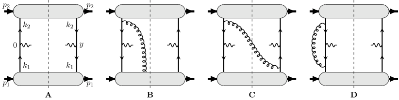
Figure 1: Example of diagrams contributing to the DY process. Gray blobs show the hadron nonperturbative state. The vertical dashed line denote the insertion of complete set of states.

The derivation of the LP term of the TMD factorization theorem has been extensively discussed in numerous references employing various formulations. Here are only some of them Mulders:1995dh ; Boer:2003cm ; Bacchetta:2006tn ; Arnold:2008kf ; Becher:2010tm ; Collins:2011zzd ; Echevarria:2011epo ; Vladimirov:2021hdn . In this section, I provide an overview of the derivation from the perspective of operator manipulations, similar to the TMD operator expansion, Soft-Collinear effective theories or High-Energy expansion. Emphasis is done on the technical aspects that are relevant for further explanations. I omit detailed proofs that can be found in the literature.

The QCD part of the cross-section for a hard reactions is given by the hadronic tensor. For the Drell-Yan process (31) the hadronic tensor reads

$$W^{\mu\nu}=\int\frac{d^{4}y}{(2\pi)^{4}}e^{-i(yq)}\sum_{X}\langle p_{1},p_{2}|J^{\mu}(y)|X\rangle\langle X|J^{\nu}(0)|p_{1},p_{2}\rangle,$$ (32)

where $J^{\mu}$ is the electromagnetic (EM) current

$$J^{\mu}(y)=\bar{q}(y)\gamma^{\mu}q(y),$$ (33)

with $q$ being the quark field. The quark charges and flavor part of the current are omitted for brevity and restored in the following sections.

The kinematics of the process is defined by the photon momentum $q^{\mu}$ and the hadrons momenta $p_{1}^{\mu}$ and $p_{2}^{\mu}$. To avoid complications related to the target mass corrections, the hadrons are considered as massless $p_{1}^{2}=p_{2}^{2}=0$. These momenta introduce the natural system of vectors $n$ and $\bar{n}$ (9)

$$p_{1}^{\mu}=\bar{n}^{\mu}p_{1}^{+},\qquad p_{2}^{\mu}=n^{\mu}p_{2}^{-}.$$ (34)

The leading perturbative order contribution to the hadronic tensor of Drell-Yan process (32) is shown in fig.1(A). This diagram and its charge-conjugated are convenient to write as

$$W^{\mu\nu} = \int\frac{d^{4}y}{(2\pi)^{4}}e^{-i(yq)}\langle p_{1}|\langle p_{2}|J^{\mu}_{\bar{n}n}(y)J^{\nu}_{n\bar{n}}(0)+J^{\mu}_{n\bar{n}}(y)J^{\nu}_{\bar{n}n}(0)|p_{1}\rangle|p_{2}\rangle+...,$$ (35)

where dots represent the sub-leading terms, and

$$J^{\mu}_{\bar{n}n}=\bar{q}_{\bar{n}}\gamma^{\mu}q_{n},\qquad J^{\mu}_{n\bar{n}}=\bar{q}_{n}\gamma^{\mu}q_{\bar{n}}.$$ (36)

The fields $q_{\bar{n}}$ ($q_{n}$) are created by $|p_{1}\rangle$ ($|p_{2}\rangle$) states, and, according to the parton model, have momentum almost along $p_{1}$($p_{2}$). Usually, fields $q_{\bar{n}}$ and $q_{n}$ are referred as collinear and anti-collinear fields. At LP approximation the states $|p_{1}\rangle$ and $|p_{2}\rangle$ do not interact with each other directly. The complete set of states in-between currents is omitted for simplicity.

To proceed further, one should specify the counting rules for the elements of equation (35). For the TMD factorization the counting rules are Becher:2010tm ; Echevarria:2011epo ; Vladimirov:2021hdn

$$\partial_{\mu}q_{\bar{n}}\sim A_{\mu,\bar{n}}\sim\{1,\lambda^{2},\lambda\},\quad\partial_{\mu}q_{n}\sim A_{\mu,n}\sim\{\lambda^{2},1,\lambda\},$$ (37)

where $\lambda\sim Q^{-1}$. The components are presented in the order $\{+,-,T\}$. In the regime $q^{\pm}\sim Q$ and $q_{T}\sim Q^{0}$ the vector $y$ satisfies the counting

$$y^{\mu}\sim Q^{-1}\{1,1,\lambda^{-1}\}$$ (38)

The inhomogeneity of counting for components of $y^{\mu}$ is the only conceptual difference between collinear and TMD factorizations.

The counting rules imply that the interactions between fields along certain directions are power-suppressed. The field must be expanded around these directions

$$q_{\bar{n}}(y)=q_{\bar{n}}(y^{-}n+y_{T})+y^{+}\partial_{-}q_{\bar{n}}(y^{-}n+y_{T})+...~{},$$ (39)

where the first term is $\sim\lambda^{0}$, the second term is $\sim\lambda^{2}$, and the dots indicate the further suppressed terms. Importantly, there is no expansion in the transverse direction, because $y^{\mu}_{T}\partial_{\mu}q_{\bar{n}}\sim\lambda^{0}$ according to (37) and (38). Meanwhile, the transverse derivatives that appear in other parts of computation (e.g. in the loops) and that are not accompanied by $y_{T}$, produce power suppressed terms.

In addition to the diagram A, one should take into account the diagrams that are of the same order of power counting. These are diagrams with radiation of collinear components of gluon, such as diagram B in fig.1. Accounting of all such diagrams restores the QCD gauge invariance and equips the collinear and anti-collinear quark fields by half-infinite Wilson lines Belitsky:2002sm ; Boer:2003cm . Practically, it is convenient to impose the light-cone gauge for the background field. The gauge can be fixed for each collinear sector such that gluon fields with a $\sim\lambda^{0}$ power counting vanish, i.e. $A_{\bar{n},+}=0$ and $A_{n,-}=0$. The detailed justification of such choice can be found e.g. in ref.Vladimirov:2021hdn . For the present work, it is enough to know that this set of gauges provides the correct factorization.

Dropping the power-suppressed terms in eqn.(39), one gets the hadronic tensor in the form

$$W^{\mu\nu} = \int\frac{d^{4}y}{(2\pi)^{4}}e^{-i(yq)}$$

$$\quad\times\langle p_{1}|\langle p_{2}|\bar{q}_{\bar{n}}(y^{-}n+y_{T})\gamma^{\mu}q_{n}(y^{+}\bar{n}+y_{T})\bar{q}_{n}(0)\gamma^{\nu}q_{\bar{n}}(0)+\{\bar{n}\leftrightarrow n\}|p_{1}\rangle|p_{2}\rangle+...~{}.$$

The central assumption of the parton model is that a high-energy hadron consists of fields with corresponding collinear counting rules. Therefore, we can sort the fields with different collinearity into separate matrix elements. To do so, one needs to recouple the spinor and color indices, which could be done using the completeness relation of Dirac matrices

$$A=\frac{1}{2}\sum_{a}\overline{\Gamma}_{a}A^{[\Gamma_{a}]},\qquad A^{[\Gamma]}=\frac{1}{2}\mathrm{Tr}\left(A\Gamma\right),$$ (41)

for any matrix $A$. Here, $\Gamma$ is a complete basis of Dirac matrices. The result reads

$$W^{\mu\nu} = -\frac{1}{4N_{c}}\int\frac{d^{4}y}{(2\pi)^{4}}e^{-i(yq)}\sum_{a,b}\Big{(}\mathrm{Tr}\left(\gamma^{\mu}\overline{\Gamma}_{b}\gamma^{\nu}\overline{\Gamma}_{a}\right)\widetilde{\Psi}_{\bar{n}}^{[\Gamma_{a}]}(y^{-}n+y_{T})\widetilde{\Psi}_{n}^{[\Gamma_{b}]}(-y^{+}\bar{n}-y_{T})$$ (42)

$$\qquad\qquad+\mathrm{Tr}\left(\gamma^{\mu}\overline{\Gamma}_{a}\gamma^{\nu}\overline{\Gamma}_{b}\right)\widetilde{\Psi}_{\bar{n}}^{[\Gamma_{a}]}(-y^{-}n-y_{T})\widetilde{\Psi}_{n}^{[\Gamma_{b}]}(y^{+}\bar{n}+y_{T})\Big{)}+...,$$

where the common minus sing appears from the anti-commutation of the quark fields, and the factor $1/N_{c}$ is due to the recoupling of color indices. The matrix elements are

$$\widetilde{\Psi}_{\bar{n}}^{[\Gamma]}(y^{-}n+y_{T})=\langle p_{1}|\bar{q}_{\bar{n}}(y^{-}n+y_{T})[y^{-}n+y_{T},-\infty n+y_{T}]\frac{\Gamma}{2}[-\infty n,0]q_{\bar{n}}(0)|p_{1}\rangle,$$ (43)

$$\widetilde{\Psi}_{n}^{[\Gamma]}(y^{+}\bar{n}+y_{T})=\langle p_{2}|\bar{q}_{n}(y^{+}\bar{n}+y_{T})[y^{+}\bar{n}+y_{T},-\infty\bar{n}+y_{T}]\frac{\Gamma}{2}[-\infty\bar{n},0]q_{n}(0)|p_{2}\rangle.$$ (44)

These distributions are Fourier images of distributions $\widetilde{\Phi}$ (2.3) over the variables $x$. In expressions (43, 44) the complete set of states in-between quark fields can be omitted because all distances are space-like.

The expression (42) is of indefinite power, because the TMD distribution $\Psi^{[\gamma^{\mu}]}$ is a mixture of terms with different power counting. It follows form eqn. (21), where the first line is $\sim\lambda^{0}$, the second and fourth lines are $\sim\lambda^{1}$, etc. Therefore, the pure LP term is obtained by eliminating all, except the first, terms in eqn.(21). It can be done by selecting only those $\Gamma$-matrices that project only “good” components. For the collinear part these matrices are

$$\Gamma^{+}_{a}=\{\gamma^{+},\gamma^{+}\gamma^{5},i\sigma^{\alpha+}\gamma^{5}\},$$ (45)

with $\alpha$ being transverse index. The corresponding elements of the basis are

$$\overline{\Gamma}^{-}_{a}=\{\gamma^{-},-\gamma^{-}\gamma^{5},-\frac{i}{2}\sigma^{\alpha-}\gamma^{5}\}.$$ (46)

For the decomposition in the anti-collinear sector one should use $\Gamma^{-}_{a}$ and $\overline{\Gamma}^{+}_{a}$ that are obtained by the replacement $n\leftrightarrow\bar{n}$ in (45) and (46), correspondingly. After restriction of $\Gamma$-matrices to the set (45) the hadronic tensor contains only the LP contribution.

Finally, one passes to the momentum-fraction representation for TMD distributions and integrates over $y^{\pm}$. The result is

$$W^{\mu\nu}_{\text{LP}}=-\frac{p_{1}^{+}p_{2}^{-}}{4N_{c}}\int\frac{d^{2}b}{(2\pi)^{2}}e^{-i(bq_{T})}\int dxd\tilde{x}\delta(xp_{1}^{+}-q^{+})\delta(\tilde{x}p_{2}^{-}-q^{-})\sum_{a,b}\Big{(}$$ (47)

$$\quad\mathrm{Tr}\left(\gamma^{\mu}\overline{\Gamma}^{+}_{b}\gamma^{\nu}\overline{\Gamma}^{-}_{a}\right)\widetilde{\Phi}_{\bar{n}11}^{[\Gamma^{+}_{a}]}(x,b)\widetilde{\Phi}_{n11}^{[\Gamma_{b}^{-}]}(-\tilde{x},-b)+\mathrm{Tr}\left(\gamma^{\mu}\overline{\Gamma}^{-}_{a}\gamma^{\nu}\overline{\Gamma}^{+}_{b}\right)\widetilde{\Phi}_{\bar{n}11}^{[\Gamma_{a}^{+}]}(-x,-b)\widetilde{\Phi}_{n11}^{[\Gamma_{b}^{-}]}(\tilde{x},b)\Big{)},$$

where $y_{T}$ is renamed as $b$, to match the standard notation. The expression (47) is the celebrated expression for the LP TMD factorization. The TMD distributions with negative $x$ are related to the anti-quark distributions.

This is a complete derivation of LP TMD factorization at the tree order. To go beyond LO, one should include interaction diagrams. Some examples are presented in fig.1. The diagrams of type B (with a non-collinear gluon) or C do not contribute to the LP factorization. Indeed, any addition interaction with the hadrons (such as fig.1B) increases the number of fields in the operator, and hence increases its dimension. The only exception is the radiation of collinear gluons, which is already accounted in the LP term. Therefore, the interactions that do not violate the power counting are possible only in-between the hard fields. Even so, some hard interactions are power suppressed, due to inhomogeneous counting rules for $y$. Indeed, the diagram 1C is $\sim 1/b^{2}$ in the position space, which leads to $\sim q_{T}^{2}/Q^{2}$ in the momentum space. Therefore, the perturbative correction at LP are given by the interactions in the vicinity of currents, such as the diagram 1D. As the result, the coefficient function is the product of coefficient functions for each current. It is in the one-to-one correspondence with the TMD-twist idea. Each semi-compact operator produces independent UV renormalization factor, that cancels the infrared poles of a corresponding part of coefficient function. This structure of pole cancellations is preserved at all powers of TMD factorization.

Finally, one should also take into account that separation of collinear and anti-collinear modes is ambiguous. For the small values of momenta the collinear and anti-collinear sectors overlap. There are several methods to avoid it. The double-counting of modes can be subtracted by means of the soft factor Manohar:2006nz ; Collins:2011zzd or rapidity renormalization factor Vladimirov:2017ksc , or modes can be defined with explicit cut parameter that prevents the overlap Balitsky:2023hmh ; Vladimirov:2021hdn . The results coincide. This procedure leads to an extra scales $\zeta$ and $\bar{\zeta}$, and corresponding evolution equations (30).

3.2 KPC for LP term at all orders

The extension of the TMD factorization beyond LP is conceptually straightforward (although very complicated technically). One should systematically expand the interaction vertices in the background fields, and sort operators over the twists and power counting. Detailed discussions are presented in refs.Vladimirov:2021hdn ; Balitsky:2020jzt . Performing this procedure, one receives the structure (3). In the following, I concentrate on the KPCs to the LP term. They are much simpler than other types of power corrections, because they incorporate only the TMD distributions of twist-two. Let me consider the series of power corrections and extract only the twist-two component from it. This component produces the complete series of KPCs.

The key observation is that the TMD distributions of twist-two are given by only two-point operators. Indeed, an insertion of any extra field increases the dimension and, thus, the TMD-twist by at least one. The geometrical-twist-three operators are all three-point operators. Such a simple rule (twist $\sim$ number of fields) does not hold for higher-twist operators starting from twist-four, which could be three-point or four-point operators Braun:2009vc . Still, one can formulate a rule: any two-point operator can contain geometrical twist-two part, but any three-point and higher-number-of-points operators necessarily have geometrical twist higher than two. It implies that any diagram with three or more particles in a single collinear sector (such as diagram B) does not contribute to KPCs for LP term. Consequently, the diagram A contains full information about twist-two part at all powers at LO in perturbative expansion.

Inspecting the LP derivation in sec. 3.1, one finds that the power corrections were dropped in two places: the multipole decomposition (39) and selection of “good” components of fields. If one does not perform these approximation the result will contain full information on KPCs. Lets release these approximations.

Starting with eqn.(35) and performing the multipole expansion one obtains

$$W^{\mu\nu}=\int\frac{d^{4}y}{(2\pi)^{4}}e^{-i(yq)}\sum_{n,m=0}^{\infty}\frac{(y^{+})^{n}(y^{-})^{m}}{n!m!}$$ (48)

$$\quad\times\langle p_{1}|\langle p_{2}|\bar{q}_{\bar{n}}(y^{-}n+y_{T})\overleftarrow{\partial_{-}}^{n}\gamma^{\mu}\overrightarrow{\partial_{+}}^{m}q_{n}(y^{+}\bar{n}+y_{T})J^{\nu}_{n\bar{n}}(0)+\{\bar{n}\leftrightarrow n\}|p_{1}\rangle|p_{2}\rangle+...\,.$$

Here, the dots represent contributions with larger number of fields. The LP term (3.1) is at $n=m=0$. Expressing the $\Gamma$-structure in the standard basis gives

$$W^{\mu\nu}=\frac{-1}{4N_{c}}\int\frac{d^{4}y}{(2\pi)^{4}}e^{-i(yq)}\sum_{a,b}\sum_{n,m=0}^{\infty}\frac{(y^{+})^{n}(y^{-})^{m}}{n!m!}\Big{[}$$ (49)

$$\quad\mathrm{Tr}\left(\gamma^{\mu}\overline{\Gamma}_{b}\gamma^{\nu}\overline{\Gamma}_{a}\right)~{}\langle p_{1}|\overline{U}_{q}(y^{-},y_{T})\overleftarrow{\partial_{-}}^{n}\frac{\Gamma_{a}}{2}U_{q}(0,0_{T})|p_{1}\rangle~{}\langle p_{2}|\overline{U}_{q}(-y^{+},-y_{T})\frac{\Gamma_{b}}{2}\overrightarrow{\partial_{+}}^{m}U_{q}(0,0_{T})|p_{2}\rangle$$

$$\qquad\qquad+\{\bar{n}\leftrightarrow n\}\Big{]}+...\,,$$

where the I use the notation (7) to highlight the semi-compact operators. Note that operators in the matrix elements with $p_{1}$($p_{2}$) are (anti-)collinear. In contrast to the LP term, there are no constraints on $\Gamma$-matrices, since any Dirac component could produce a twist-two contribution, see example in eqn. (23).

The semi-compact operators in eqn.(49) contain the mixture of TMD distribution, and should be decomposed over the definite twist contributions. For the pure $U_{q}$ operators the decomposition is given in eqn.(18). However, the “improper” derivatives of $U_{q}$ (such as $\partial_{-}q_{\bar{n}}$) demolish this decomposition because they could not be presented as total derivatives of distributions. This issue is resolved by application of EOMs (15). The analysis of these operators is complicated in the general case, but essentially simpler if one seeks for only twist-one contribution. In this case, all gluon fields in EOMs could be dropped (since gluon-fields necessarily turn one-point operator to a higher-number-of-points operators), resulting to a simple rule

$$\partial_{-}\xi_{\bar{n}}=-\frac{\partial_{T}^{2}}{2\partial_{+}}\xi_{\bar{n}}+...,\qquad\partial_{-}\eta_{\bar{n}}=\frac{\gamma^{+}\not{\partial}_{T}\partial_{T}^{2}}{4\partial^{2}_{+}}\xi_{\bar{n}}+...~{},$$ (50)

where dots represent the terms with two or larger number of fields. Here inverse derivatives are understood as the integral, alike (17). Basically, the equation (50) tells that at the leading-twist approximation partons are free massless fields. The higher powers of $\partial_{-}$ are

$$\partial_{-}^{n}\xi_{\bar{n}}=\left(-\frac{\partial_{T}^{2}}{2\partial_{+}}\right)^{n}\xi_{\bar{n}}+...,\qquad\partial^{n}_{-}\eta_{\bar{n}}=-\frac{\gamma^{+}\not{\partial}_{T}}{2\partial_{+}}\left(-\frac{\partial_{T}^{2}}{2\partial_{+}}\right)^{n}\xi_{\bar{n}}+...~{}.$$ (51)

After these transformations, the fields $\xi$ could be promoted to the semi-compact operators $U_{1}$, by equipping them by semi-infinite Wilson lines, as it is demanded by the QCD gauge invariance.

As a result of these manipulations, one obtains a long expression

$$W_{\text{KPC}}^{\mu\nu} = \frac{-1}{4N_{c}}\int\frac{d^{4}y}{(2\pi)^{4}}e^{-i(yq)}\sum_{a,b}\sum_{n,m=0}^{\infty}\frac{(y^{+})^{n}(y^{-})^{m}}{n!m!}\frac{(-1)^{n+m}}{2^{n+m}}\Bigg{\{}$$

$$\mathrm{Tr}[\gamma_{T}^{\mu}\overline{\Gamma}_{b}^{+}\gamma_{T}^{\nu}\overline{\Gamma}_{a}^{-}]\;\frac{\partial_{T}^{2n}}{\partial_{+}^{n}}\widetilde{\Psi}_{\bar{n}11}^{[\Gamma_{a}^{+}]}\;\frac{\partial_{T}^{2m}}{\partial_{-}^{m}}\widetilde{\Psi}_{n11}^{[\Gamma_{b}^{-}]}$$

$$-\left(n^{\nu}\mathrm{Tr}[\gamma_{T}^{\mu}\overline{\Gamma}_{b}^{+}\gamma_{T}^{\alpha}\overline{\Gamma}_{a}^{-}]+n^{\mu}\mathrm{Tr}[\gamma_{T}^{\alpha}\overline{\Gamma}_{b}^{+}\gamma_{T}^{\nu}\overline{\Gamma}_{a}^{-}]\right)\frac{\partial_{\alpha}}{\partial_{+}}\frac{\partial_{T}^{2n}}{\partial_{+}^{n}}\widetilde{\Psi}_{\bar{n}11}^{[\Gamma_{a}^{+}]}\;\frac{\partial_{T}^{2m}}{\partial_{-}^{m}}\widetilde{\Psi}_{n11}^{[\Gamma_{b}^{-}]}$$

$$-\left(\bar{n}^{\nu}\mathrm{Tr}[\gamma_{T}^{\mu}\overline{\Gamma}_{b}^{+}\gamma_{T}^{\alpha}\overline{\Gamma}_{a}^{-}]+\bar{n}^{\mu}\mathrm{Tr}[\gamma_{T}^{\alpha}\overline{\Gamma}_{b}^{+}\gamma_{T}^{\nu}\overline{\Gamma}_{a}^{-}]\right)\frac{\partial_{T}^{2n}}{\partial_{+}^{n}}\widetilde{\Psi}_{\bar{n}11}^{[\Gamma_{a}^{+}]}\;\frac{\partial_{\alpha}}{\partial_{-}}\frac{\partial_{T}^{2m}}{\partial_{-}^{m}}\widetilde{\Psi}_{n11}^{[\Gamma_{b}^{-}]}$$

$$-\frac{1}{2}\left(\mathrm{Tr}[\gamma_{T}^{\mu}\overline{\Gamma}_{b}^{+}\gamma_{T}^{\beta}\gamma_{T}^{\nu}\gamma^{\alpha}_{T}\overline{\Gamma}_{a}^{-}]+\mathrm{Tr}[\gamma_{T}^{\alpha}\gamma_{T}^{\mu}\gamma^{\beta}_{T}\overline{\Gamma}_{b}^{+}\gamma_{T}^{\nu}\overline{\Gamma}_{a}^{-}]\right)\frac{\partial_{\alpha}}{\partial_{+}}\frac{\partial_{T}^{2n}}{\partial_{+}^{n}}\widetilde{\Psi}_{\bar{n}11}^{[\Gamma_{a}^{+}]}\;\frac{\partial_{\beta}}{\partial_{-}}\frac{\partial_{T}^{2m}}{\partial_{-}^{m}}\widetilde{\Psi}_{n11}^{[\Gamma_{b}^{-}]}$$

$$+\left(\bar{n}^{\mu}n^{\nu}\mathrm{Tr}[\gamma_{T}^{\beta}\overline{\Gamma}_{b}^{+}\gamma^{\alpha}_{T}\overline{\Gamma}_{a}^{-}]+n^{\mu}\bar{n}^{\nu}\mathrm{Tr}[\gamma_{T}^{\alpha}\overline{\Gamma}_{b}^{+}\gamma^{\beta}_{T}\overline{\Gamma}_{a}^{-}]\right)\frac{\partial_{\alpha}}{\partial_{+}}\frac{\partial_{T}^{2n}}{\partial_{+}^{n}}\widetilde{\Psi}_{\bar{n}11}^{[\Gamma_{a}^{+}]}\;\frac{\partial_{\beta}}{\partial_{-}}\frac{\partial_{T}^{2m}}{\partial_{-}^{m}}\widetilde{\Psi}_{n11}^{[\Gamma_{b}^{-}]}$$

$$+\mathrm{Tr}[\gamma_{T}^{\alpha}\overline{\Gamma}_{b}^{+}\gamma^{\beta}_{T}\overline{\Gamma}_{a}^{-}]\left(\bar{n}^{\mu}\bar{n}^{\nu}\frac{\partial_{T}^{2n}}{\partial_{+}^{n}}\widetilde{\Psi}_{\bar{n}11}^{[\Gamma_{a}^{+}]}\;\frac{\partial_{\alpha}}{\partial_{-}}\frac{\partial_{\beta}}{\partial_{-}}\frac{\partial_{T}^{2m}}{\partial_{-}^{m}}\widetilde{\Psi}_{n11}^{[\Gamma_{b}^{-}]}+n^{\mu}n^{\nu}\frac{\partial_{\alpha}}{\partial_{+}}\frac{\partial_{\beta}}{\partial_{+}}\frac{\partial_{T}^{2n}}{\partial_{+}^{n}}\widetilde{\Psi}_{\bar{n}11}^{[\Gamma_{a}^{+}]}\;\frac{\partial_{T}^{2m}}{\partial_{-}^{m}}\widetilde{\Psi}_{n11}^{[\Gamma_{b}^{-}]}\right)$$

$$+\frac{1}{2}\left(\bar{n}^{\mu}\mathrm{Tr}[\gamma_{T}^{\sigma}\overline{\Gamma}_{b}^{+}\gamma^{\beta}_{T}\gamma^{\nu}\gamma^{\alpha}\overline{\Gamma}_{a}^{-}]+\bar{n}^{\nu}\mathrm{Tr}[\gamma^{\alpha}_{T}\gamma_{T}^{\mu}\gamma^{\beta}_{T}\overline{\Gamma}_{b}^{+}\gamma^{\sigma}_{T}\overline{\Gamma}_{a}^{-}]\right)\frac{\partial_{\alpha}}{\partial_{+}}\frac{\partial_{T}^{2n}}{\partial_{+}^{n}}\widetilde{\Psi}_{\bar{n}11}^{[\Gamma_{a}^{+}]}\;\frac{\partial_{\beta}}{\partial_{-}}\frac{\partial_{\sigma}}{\partial_{-}}\frac{\partial_{T}^{2m}}{\partial_{-}^{m}}\widetilde{\Psi}_{n11}^{[\Gamma_{b}^{-}]}$$

$$+\frac{1}{2}\left(n^{\mu}\mathrm{Tr}[\gamma_{T}^{\alpha}\overline{\Gamma}_{b}^{+}\gamma^{\sigma}_{T}\gamma^{\nu}\gamma^{\beta}\overline{\Gamma}_{a}^{-}]+n^{\nu}\mathrm{Tr}[\gamma^{\beta}_{T}\gamma_{T}^{\mu}\gamma^{\sigma}_{T}\overline{\Gamma}_{b}^{+}\gamma^{\alpha}_{T}\overline{\Gamma}_{a}^{-}]\right)\frac{\partial_{\alpha}}{\partial_{+}}\frac{\partial_{\beta}}{\partial_{+}}\frac{\partial_{T}^{2n}}{\partial_{+}^{n}}\widetilde{\Psi}_{\bar{n}11}^{[\Gamma_{a}^{+}]}\;\frac{\partial_{\sigma}}{\partial_{-}}\frac{\partial_{T}^{2m}}{\partial_{-}^{m}}\widetilde{\Psi}_{n11}^{[\Gamma_{b}^{-}]}$$

$$+\frac{1}{4}\mathrm{Tr}[\gamma_{T}^{\alpha}\gamma^{\mu}_{T}\gamma_{T}^{\sigma}\overline{\Gamma}_{b}^{+}\gamma^{\rho}_{T}\gamma^{\nu}\gamma_{T}^{\beta}\overline{\Gamma}_{a}^{-}]\frac{\partial_{\alpha}}{\partial_{+}}\frac{\partial_{\beta}}{\partial_{+}}\frac{\partial_{T}^{2n}}{\partial_{+}^{n}}\widetilde{\Psi}_{\bar{n}11}^{[\Gamma_{a}^{+}]}\;\frac{\partial_{\sigma}}{\partial_{-}}\frac{\partial_{\rho}}{\partial_{-}}\frac{\partial_{T}^{2m}}{\partial_{-}^{m}}\widetilde{\Psi}_{n11}^{[\Gamma_{b}^{-}]}\Bigg{\}}+(n\leftrightarrow\bar{n}),$$

where the argument of $\widetilde{\Psi}_{\bar{n}11}$ is $(y^{-}n+y_{T})$, and the argument of $\widetilde{\Psi}_{n11}$ is $(-y^{+}\bar{n}-y_{T})$. This expression contains all twist-two terms of TMD factorization that appear at LO in perturbation theory. The eliminated terms have higher twist.

Finally, one integrates over $y^{\pm}$ and obtains

$$W_{\text{KPC}}^{\mu\nu}=\frac{-p_{1}^{+}p_{2}^{-}}{4N_{c}}\int\frac{d^{2}b}{(2\pi)^{2}}e^{-i(bq_{T})}\int dxd\tilde{x}\delta(xp_{1}^{+}-q^{+})\delta(\tilde{x}p_{2}^{-}-q^{-})$$ (53)

$$\sum_{q,\bar{q}}\sum_{a,b}\sum_{n,m=0}^{\infty}\frac{\partial_{\tilde{x}}^{n}\partial_{x}^{m}}{n!m!}\frac{(-1)^{n+m}}{(2p_{1}^{+}p_{2}^{-})^{n+m}}\frac{1}{x^{n}\tilde{x}^{m}}\Bigg{\{}$$

$$\mathrm{Tr}[\gamma_{T}^{\mu}\overline{\Gamma}_{b}^{+}\gamma_{T}^{\nu}\overline{\Gamma}_{a}^{-}]\;\partial_{T}^{2n}\widetilde{\Phi}_{\bar{n}11}^{[\Gamma_{a}^{+}]}\;\partial_{T}^{2m}\widetilde{\Phi}_{n11}^{[\Gamma_{b}^{-}]}$$

$$+\frac{i}{xp_{1}^{+}}\left(n^{\nu}\mathrm{Tr}[\gamma_{T}^{\mu}\overline{\Gamma}_{b}^{+}\gamma_{T}^{\alpha}\overline{\Gamma}_{a}^{-}]+n^{\mu}\mathrm{Tr}[\gamma_{T}^{\alpha}\overline{\Gamma}_{b}^{+}\gamma_{T}^{\nu}\overline{\Gamma}_{a}^{-}]\right)\partial_{\alpha}\partial_{T}^{2n}\widetilde{\Phi}_{\bar{n}11}^{[\Gamma_{a}^{+}]}\;\partial_{T}^{2m}\widetilde{\Phi}_{n11}^{[\Gamma_{b}^{-}]}$$

$$+\frac{i}{\tilde{x}p_{2}^{-}}\left(\bar{n}^{\nu}\mathrm{Tr}[\gamma_{T}^{\mu}\overline{\Gamma}_{b}^{+}\gamma_{T}^{\alpha}\overline{\Gamma}_{a}^{-}]+\bar{n}^{\mu}\mathrm{Tr}[\gamma_{T}^{\alpha}\overline{\Gamma}_{b}^{+}\gamma_{T}^{\nu}\overline{\Gamma}_{a}^{-}]\right)\partial_{T}^{2n}\widetilde{\Phi}_{\bar{n}11}^{[\Gamma_{a}^{+}]}\;\partial_{\alpha}\partial_{T}^{2m}\widetilde{\Phi}_{n11}^{[\Gamma_{b}^{-}]}$$

$$+\frac{1}{2x\tilde{x}p_{1}^{+}p_{2}^{-}}\Big{(}\mathrm{Tr}[\gamma_{T}^{\mu}\overline{\Gamma}_{b}^{+}\gamma_{T}^{\beta}\gamma_{T}^{\nu}\gamma^{\alpha}_{T}\overline{\Gamma}_{a}^{-}]+\mathrm{Tr}[\gamma_{T}^{\alpha}\gamma_{T}^{\mu}\gamma^{\beta}_{T}\overline{\Gamma}_{b}^{+}\gamma_{T}^{\nu}\overline{\Gamma}_{a}^{-}]$$

$$\qquad\qquad+2\bar{n}^{\mu}n^{\nu}\mathrm{Tr}[\gamma_{T}^{\beta}\overline{\Gamma}_{b}^{+}\gamma^{\alpha}_{T}\overline{\Gamma}_{a}^{-}]+2n^{\mu}\bar{n}^{\nu}\mathrm{Tr}[\gamma_{T}^{\alpha}\overline{\Gamma}_{b}^{+}\gamma^{\beta}_{T}\overline{\Gamma}_{a}^{-}]\Big{)}\partial_{\alpha}\partial_{T}^{2n}\widetilde{\Phi}_{\bar{n}11}^{[\Gamma_{a}^{+}]}\;\partial_{\beta}\partial_{T}^{2m}\widetilde{\Phi}_{n11}^{[\Gamma_{b}^{-}]}$$

$$-\mathrm{Tr}[\gamma_{T}^{\alpha}\overline{\Gamma}_{b}^{+}\gamma^{\beta}_{T}\overline{\Gamma}_{a}^{-}]\left(\frac{\bar{n}^{\mu}\bar{n}^{\nu}}{\tilde{x}^{2}(p_{2}^{-})^{2}}\partial_{T}^{2n}\widetilde{\Phi}_{\bar{n}11}^{[\Gamma_{a}^{+}]}\;\partial_{\alpha}\partial_{\beta}\partial_{T}^{2m}\widetilde{\Phi}_{n11}^{[\Gamma_{b}^{-}]}+\frac{n^{\mu}n^{\nu}}{x^{2}(p_{1}^{+})^{2}}\partial_{\alpha}\partial_{\beta}\partial_{T}^{2n}\widetilde{\Phi}_{\bar{n}11}^{[\Gamma_{a}^{+}]}\;\partial_{T}^{2m}\widetilde{\Phi}_{n11}^{[\Gamma_{b}^{-}]}\right)$$

$$+\frac{i}{2x\tilde{x}^{2}p_{1}^{+}(p_{2}^{-})^{2}}\left(\bar{n}^{\mu}\mathrm{Tr}[\gamma_{T}^{\sigma}\overline{\Gamma}_{b}^{+}\gamma^{\beta}_{T}\gamma^{\nu}\gamma^{\alpha}\overline{\Gamma}_{a}^{-}]+\bar{n}^{\nu}\mathrm{Tr}[\gamma^{\alpha}_{T}\gamma_{T}^{\mu}\gamma^{\beta}_{T}\overline{\Gamma}_{b}^{+}\gamma^{\sigma}_{T}\overline{\Gamma}_{a}^{-}]\right)\partial_{\alpha}\partial_{T}^{2n}\widetilde{\Phi}_{\bar{n}11}^{[\Gamma_{a}^{+}]}\;\partial_{\beta}\partial_{\sigma}\partial_{T}^{2m}\widetilde{\Phi}_{n11}^{[\Gamma_{b}^{-}]}$$

$$+\frac{i}{2x^{2}\tilde{x}(p_{1}^{+})^{2}p_{2}^{-}}\left(n^{\mu}\mathrm{Tr}[\gamma_{T}^{\alpha}\overline{\Gamma}_{b}^{+}\gamma^{\sigma}_{T}\gamma^{\nu}\gamma^{\beta}\overline{\Gamma}_{a}^{-}]+n^{\nu}\mathrm{Tr}[\gamma^{\beta}_{T}\gamma_{T}^{\mu}\gamma^{\sigma}_{T}\overline{\Gamma}_{b}^{+}\gamma^{\alpha}_{T}\overline{\Gamma}_{a}^{-}]\right)\partial_{\alpha}\partial_{\beta}\partial_{T}^{2n}\widetilde{\Phi}_{\bar{n}11}^{[\Gamma_{a}^{+}]}\;\partial_{\sigma}\partial_{T}^{2m}\widetilde{\Phi}_{n11}^{[\Gamma_{b}^{-}]}$$

$$+\frac{1}{4(x\tilde{x}p_{1}^{+}p_{2}^{-})^{2}}\mathrm{Tr}[\gamma_{T}^{\alpha}\gamma^{\mu}_{T}\gamma_{T}^{\sigma}\overline{\Gamma}_{b}^{+}\gamma^{\rho}_{T}\gamma^{\nu}\gamma_{T}^{\beta}\overline{\Gamma}_{a}^{-}]\partial_{\alpha}\partial_{\beta}\partial_{T}^{2n}\widetilde{\Phi}_{\bar{n}11}^{[\Gamma_{a}^{+}]}\;\partial_{\sigma}\partial_{\rho}\partial_{T}^{2m}\widetilde{\Phi}_{n11}^{[\Gamma_{b}^{-}]}\Bigg{\}},$$

where arguments of the TMD-distributions are $(x,b)$ for $\widetilde{\Phi}_{\bar{n}11}$ and $(\tilde{x},b)$ for $\widetilde{\Phi}_{n11}$. The derivatives $\partial_{x}=\frac{\partial}{\partial x}$ ($\partial_{\tilde{x}}=\frac{\partial}{\partial\tilde{x}}$) comes from from the integration over $y^{-}$($y^{+}$). Herewith, distributions $\widetilde{\Phi}_{\bar{n}11}$ are quark distributions and $\widetilde{\Phi}_{n11}$ are anti-quark distributions. The sum $\sum_{q,\bar{q}}$ indicates the addition of the term with quark and anti-quark distributions exchanged. This expression is valid for any polarizations. The example of unpolarized cases are given in sec. 5. In particular, the LP expression is given in eqn.(95), NLP in eqn.(5), and NNLP in eqn.(5). The NLP part of eqn.(53) exactly reproduces the KPC-part of the full NLP expression derived in ref.Vladimirov:2021hdn ; Balitsky:2020jzt .

It is complicated to investigate the properties (53) in the general form. However, one can confirm that the expression (53) is exactly EM-gauge invariant,

$$q_{\mu}W_{\text{KPC}}^{\mu\nu}=0.$$ (54)

The truncated at NⁿLP order part of series (53) is not transverse, but violates EM-gauge invariance up to order Nⁿ⁺¹LP. The exact restoration involves all terms. Moreover, the series (53) could not be split into independently gauge-invariant parts or at least such a split is not natural. The terms with derivatives $\partial_{x}$ and $\partial_{\tilde{x}}$ play important role in the restoration of gauge invariance, since they (after integration by parts) turn $q^{\pm}$ to $p^{\pm}$, which is required for the cancellation between different orders. The expression (53) is also frame-invariant, although it is complicated to confirm. These invariances are discussed explicitly with the unpolarized example in sec. 5.1 and sec. 5.2, and they are obvious in the summed form (4.2).

3.3 KPCs beyond LO and the argument of the coefficient function

In the present approximation (solely twist-two TMD operators, neglecting $q_{T}/Q$ corrections) the perturbative corrections come only from the corrections to the EM currents. Indeed, an inclusion of a non-collinear external gluon increases the twist of operators, and the in-between currents interaction (alike fig.1C) induces $q_{T}/Q$ corrections. Therefore, one can consider perturbative corrections for the currents $J_{\bar{n}n}$ and $J_{n\bar{n}}$ (36) independently. The NLO LP computation the coefficient function is performed in multiple works, see f.i. refs.Collins:2011zzd ; Echevarria:2011epo ; Becher:2010tm ; Manohar:2003vb ; Vladimirov:2021hdn . Presently, it is known up to N⁴LO accuracy (4-loop) Lee:2022nhh ; Moult:2022xzt . The NLP NLO computation has been done explicitly in ref.Vladimirov:2021hdn , and the result coincides with LP. It is a non-trivial check since, intermediate expressions and the algebra of NLP computation are different from those at LP (see the detailed discussion in sec.6 of ref.Vladimirov:2021hdn ). As it is explained above, the coefficient function of KPC must be the same as the LP coefficient function. In this section I would like to confirm it by explicit computation.

The perturbative computations beyond LP are much simpler in the position space. It is because Feynman propagators in the position space are free of external momenta, which appear only in the numerator of diagrams. Therefore, one should not worry about increasing singularity of power suppressed parts of integrals as it happen in the momentum space. The explanation of convenient technique for loop-computation with multiple examples can be found f.i. in refs. Vladimirov:2021hdn ; Balitsky:1987bk ; Scimemi:2019gge ; Braun:2021aon .

The NLO correction for EM current is given by the diagram shown in fig.1 D. In the position space, this diagram (here for $J_{\bar{n}n}(0)$) reads

diag $$= g^{2}C_{F}\frac{\Gamma^{2}(2-\epsilon)\Gamma(1-\epsilon)}{16\pi^{d/2}}\int d^{d}xd^{d}z\frac{\bar{q}_{\bar{n}}(x)\gamma^{\nu}\not{x}\gamma^{\mu}\not{z}\gamma_{\nu}q_{n}(z)}{[-x^{2}+i0]^{2-\epsilon}[-z^{2}+i0]^{2-\epsilon}[-(x-z)^{2}+i0]^{1-\epsilon}},~{}~{}$$ (55)

where $C_{F}=(N_{c}^{2}-1)/(2N_{c})$ and $d=4-2\epsilon$ is the parameter of the dimensional regularization. This expression incorporates operators of all powers and twists. The power expansion is obtained from the decomposition of external quark fields over “good” and “bad” components, and their expansion in the vicinity of the collinear direction. Importantly, the power expansion can be done at the level of the integrand (since integral is convergent due to the dimensional regularization). In this way, the only complications of higher-power computation is the increasing (from power to power) size of the numerator.

The LP and NLP computation has been carried out in ref.Vladimirov:2021hdn . It is convenient to write the result in the mixed momentum-coordinate representation

$$\text{diag}_{\text{LP}} = \frac{a_{s}C(\epsilon)}{(-2k_{1}^{+}k_{2}^{-})^{\epsilon}}\bar{\xi}_{\bar{n}}\gamma_{T}^{\mu}\xi_{n},$$ (56)

$$\text{diag}_{\text{NLP}} = \frac{a_{s}C(\epsilon)}{(-2k_{1}^{+}k_{2}^{-})^{\epsilon}}\left(-n^{\mu}\bar{\xi}_{\bar{n}}\frac{\overleftarrow{\not{\partial}}_{T}}{\overleftarrow{\partial}_{+}}\xi_{n}-\bar{n}^{\mu}\bar{\xi}_{\bar{n}}\frac{\overrightarrow{\not{\partial}}_{T}}{\overrightarrow{\partial}_{+}}\xi_{n}\right)$$ (57)

where

$$C(\epsilon)=2C_{F}\frac{\Gamma(\epsilon)\Gamma(-\epsilon)\Gamma(2-\epsilon)}{\Gamma(3-2\epsilon)}(2-\epsilon+2\epsilon^{2}),$$ (58)

and $k_{1}$ and $k_{2}$ are the momenta of quark fields $\bar{q}_{\bar{n}}$ and $q_{n}$ (in the position space they appear as derivatives). The terms (56) and (57) provide the coefficient function for the LP and NLP parts EM-current. In this way, one confirms that the coefficient function of KPC at NLP is the same as for LP term (at least at NLO).

The coefficient $C(\epsilon)$ contains infra-red divergences (since $J^{\mu}$ is a conserved current, $C(\epsilon)$ is UV finite). These divergences are compensated by the UV renormalization factors of operators $U_{1}$. These factors are $Z_{U1}$ for $U_{1}$ (anti-collinear) and $Z_{U1}^{\dagger}$ for $\overline{U}_{1}$ (collinear). These factors contain collinear divergence, which is removed by the analogous divergence in the rapidity renormalization. The LO expression for $Z_{U1}$ is

$$Z_{U1}(\zeta)=1+\frac{a_{s}C_{F}}{\epsilon}\left(\frac{1}{\epsilon}+\frac{3}{2}+\ln\left(\frac{\mu^{2}}{\zeta}\right)\right)+\mathcal{O}(a_{s}^{2}),$$ (59)

where $\zeta$ is the scale of the rapidity renormalization. Performing the renormalization procedure, one obtains

$$(1+a_{s}C(\epsilon)+\mathcal{O}(a_{s}^{2}))Z^{\dagger}_{U1}(\zeta)Z_{U1}(\bar{\zeta})=C_{V},$$ (60)

where $a_{s}=g^{2}/(4\pi)^{2}$. Importantly, for the cancellation of poles one must impose $\zeta\bar{\zeta}=(2q^{+}q^{-})^{2}$, where it is used that $k_{1}^{+}=q^{+}$ and $k_{2}^{-}=q^{-}$ due to the $\delta$-functions (47). The coefficient function $C_{V}$ is

$$C_{V}=1+a_{s}C_{F}\left(-\mathbf{L}^{2}+3\mathbf{L}-8+\frac{\pi^{2}}{6}\right)+\mathcal{O}(a_{s}^{2}),$$ (61)

where $\mathbf{L}=\ln(-2q^{+}q^{-}/\mu^{2})$. The coefficient function is multiplicative. The product of current has the coefficient function

$$C_{0}=|C_{V}|^{2}=1+2a_{s}C_{F}\left(-|\mathbf{L}|^{2}+3|\mathbf{L}|-8+\frac{7\pi^{2}}{6}\right)+\mathcal{O}(a_{s}^{2}),$$ (62)

where it has been taken into account that $q^{+}q^{-}>0$.

Let me emphasize that the argument of the coefficient function is $2q^{+}q^{-}$. This is the result of the formal computation in the factorization approach (see e.g. Vladimirov:2021hdn ; Manohar:2003vb ). Often, the argument of coefficient function at LP is replaced by $q^{2}$ for simplicity. However, it is not entirely correct since $q^{2}=2q^{+}q^{-}+q_{T}^{2}$ has an indefinite power counting.

The NLO computation can be easily automatized (necessary integrals in general form are given in appendix B or ref.Vladimirov:2021hdn ). Using the package FeynCalc Shtabovenko:2020gxv , I have generated the first few powers. They are

$$\text{diag}_{\text{N${}^{2}$LP}} = \frac{a_{s}C(\epsilon)}{(-2k_{1}^{+}k_{2}^{-})^{\epsilon}}\Big{[}-\frac{1}{2}\bar{\xi}_{\bar{n}}\frac{\overleftarrow{\not{\partial}}_{T}}{\overleftarrow{\partial}_{+}}\gamma_{T}^{\mu}\frac{\overrightarrow{\not{\partial}}_{T}}{\overrightarrow{\partial}_{+}}\xi_{n}-\epsilon\frac{(k_{1}k_{2})_{T}}{k_{1}^{+}k_{2}^{-}}\bar{\xi}_{\bar{n}}\gamma_{T}^{\mu}\xi_{n}\Big{]},$$ (63)

$$\text{diag}_{\text{N${}^{3}$LP}} = \frac{a_{s}C(\epsilon)}{(-2k_{1}^{+}k_{2}^{-})^{\epsilon}}\left(-\epsilon\frac{(k_{1}k_{2})_{T}}{k_{1}^{+}k_{2}^{-}}\right)\left(-n^{\mu}\bar{\xi}_{\bar{n}}\frac{\overleftarrow{\not{\partial}}_{T}}{\overleftarrow{\partial}_{+}}\xi_{n}-\bar{n}^{\mu}\bar{\xi}_{\bar{n}}\frac{\overrightarrow{\not{\partial}}_{T}}{\overrightarrow{\partial}_{+}}\xi_{n}\right),$$

$$\text{diag}_{\text{N${}^{4}$LP}} = \frac{a_{s}C(\epsilon)}{(-2k_{1}^{+}k_{2}^{-})^{\epsilon}}\Big{[}\frac{\epsilon}{2}\frac{(k_{1}k_{2})_{T}}{k_{1}^{+}k_{2}^{-}}\bar{\xi}_{\bar{n}}\frac{\overleftarrow{\not{\partial}}_{T}}{\overleftarrow{\partial}_{+}}\gamma_{T}^{\mu}\frac{\overrightarrow{\not{\partial}}_{T}}{\overrightarrow{\partial}_{+}}\xi_{n}+\left(\frac{\epsilon(1+\epsilon)}{2}\frac{(k_{1}k_{2})_{T}}{k_{1}^{+}k_{2}^{-}}-\frac{\epsilon}{4}\frac{k_{1T}^{2}k_{2T}^{2}}{(k_{1}^{+}k_{2}^{-})^{2}}\right)\bar{\xi}_{\bar{n}}\gamma_{T}^{\mu}\xi_{n}\Big{]},$$

$$\text{diag}_{\text{N${}^{5}$LP}} = \frac{a_{s}C(\epsilon)}{(-2k_{1}^{+}k_{2}^{-})^{\epsilon}}\left(\frac{\epsilon(1+\epsilon)}{2}\frac{(k_{1}k_{2})^{2}_{T}}{(k_{1}^{+}k_{2}^{-})^{2}}-\frac{\epsilon}{4}\frac{k_{1T}^{2}k_{2T}^{2}}{(k_{1}^{+}k_{2}^{-})^{2}}\right)\left(-n^{\mu}\bar{\xi}_{\bar{n}}\frac{\overleftarrow{\not{\partial}}_{T}}{\overleftarrow{\partial}_{+}}\xi_{n}-\bar{n}^{\mu}\bar{\xi}_{\bar{n}}\frac{\overrightarrow{\not{\partial}}_{T}}{\overrightarrow{\partial}_{+}}\xi_{n}\right),$$

$$\text{diag}_{\text{N${}^{6}$LP}} = \frac{a_{s}C(\epsilon)}{(-2k_{1}^{+}k_{2}^{-})^{\epsilon}}\Big{[}\left(\frac{\epsilon(1+\epsilon)}{2}\frac{(k_{1}k_{2})^{2}_{T}}{(k_{1}^{+}k_{2}^{-})^{2}}-\frac{\epsilon}{4}\frac{k_{1T}^{2}k_{2T}^{2}}{(k_{1}^{+}k_{2}^{-})^{2}}\right)\bar{\xi}_{\bar{n}}\frac{\overleftarrow{\not{\partial}}_{T}}{\overleftarrow{\partial}_{+}}\gamma_{T}^{\mu}\frac{\overrightarrow{\not{\partial}}_{T}}{\overrightarrow{\partial}_{+}}\xi_{n}$$

$$+\left(-\frac{\epsilon(1+\epsilon)(2+\epsilon)}{6}\frac{(k_{1}k_{2})^{3}_{T}}{(k_{1}^{+}k_{2}^{-})^{3}}-\frac{\epsilon(1+\epsilon)}{4}\frac{k_{1T}^{2}k_{2T}^{2}(k_{1}k_{2})_{T}}{(k_{1}^{+}k_{2}^{-})^{3}}\right)\bar{\xi}_{\bar{n}}\gamma_{T}^{\mu}\xi_{n}\Big{]},$$

and so on. For the convincingness, the computation has been performed up to N¹⁰LP, and it reproduces the presented pattern.

At the first glance, expressions (63) demonstrate the violation of the factorization theorem. Indeed, naively, one should expect to obtain the effective current (65) multiplied by $C(\epsilon)$. I.e. all terms except the first for $\text{diag}_{\text{N${}^{2}$LP}}$ should vanish. Instead, the expressions contain the new terms, equipped by different coefficients. It is especially confusing that these new terms have different order of $\epsilon$ singularities. Due to the latter, these terms cannot be renormalized by $Z_{U1}$’s (60), and the factorization theorem seems to be violated at NNLP and higher.

Further inspection of corrections (63) reveals a certain pattern. The all-power series (63) can be rewritten as

$$\sum_{k=0}^{\infty}\text{diag}_{\text{N${}^{k}$LP}} = \frac{a_{s}C(\epsilon)}{\left(-2k_{1}^{+}k_{2}^{-}-2(k_{1}k_{2})_{T}-\frac{k_{1T}^{2}k_{2T}^{2}}{2k_{1}^{+}k_{2}^{-}}\right)^{\epsilon}}J^{\text{tw2}}_{\bar{n}n},$$ (64)

where

$$J^{\text{tw2}}_{\bar{n}n} = \bar{\xi}_{\bar{n}}\gamma_{T}^{\mu}\xi_{n}-n^{\mu}\bar{\xi}_{\bar{n}}\frac{\overleftarrow{\not{\partial}}_{T}}{\overleftarrow{\partial}_{+}}\xi_{n}-\bar{n}^{\mu}\bar{\xi}_{\bar{n}}\frac{\overrightarrow{\not{\partial}}_{T}}{\overrightarrow{\partial}_{+}}\xi_{n}-\frac{1}{2}\bar{\xi}_{\bar{n}}\frac{\overleftarrow{\not{\partial}}_{T}}{\overleftarrow{\partial}_{+}}\gamma_{T}^{\mu}\frac{\overrightarrow{\not{\partial}}_{T}}{\overrightarrow{\partial}_{+}}\xi_{n},$$ (65)

is the twist-two part of the EM current. Therefore, the coefficient function for all KPCs is the same, but has a different argument. The argument of the coefficient function is

$$X=(2q^{+}q^{-}-2(k_{1}k_{2})_{T}-k_{1T}^{2}k_{2T}^{2}/(2q^{+}q^{-})),$$ (66)

instead of $2q^{+}q^{-}$, that appears at LP and NLP cases. The cancellation of poles also imposes

$$\zeta\bar{\zeta}=X^{2}.$$

The coefficient function $C_{0}(X)$ can be used only as the whole, because any strict fixed-power expansion would lead to the non-cancellation of poles between infra-red poles of coefficient function, and UV poles of twist-one operators. To my best knowledge, it is the first example of accumulation of power corrections into the argument of the coefficient function in factorization theorems. In sec. 4.2, it is shown that $X^{2}$ turns to $Q^{2}$ once KPCs are summed.

In the position space the variables $k_{1,2}$ are represented by the differential operators. Therefore, in the position space, the coefficient function (64) is a differential operator in the transverse space. That is the main reasons to switch to the momentum space in the following discussions.

Another contribution that reveals only beyond LO is the restoration of the boost-invariance. The boost-invariance demands that the factorization theorem is independent of the values of $\zeta$’s as far as $\zeta\bar{\zeta}=X^{2}$ (this can be demonstrated using different approaches Collins:2012ss ; Echevarria:2012js ; Vladimirov:2017ksc ). Therefore, the factorized expression should be invariant under

$$\zeta\to\alpha\zeta,\qquad\bar{\zeta}\to\alpha^{-1}\bar{\zeta},$$ (67)

at each given power. The expression (53) does not preserve this property. Indeed, the combinations with transverse derivatives, such as $\Phi_{\bar{n}}(\zeta)\partial_{T\mu}\Phi_{n}(\bar{\zeta})$ are not invariant but produces the terms $\sim(\alpha-1)\partial_{\mu}\mathcal{D}$ (for $\alpha\sim 1$), where $\mathcal{D}$ is the Collins-Soper kernel (30).

The restoration of the boost-invariance happens with the accounting of the higher-twist terms. The higher-twist distributions appears in the factorized expressions with the divergent convolution. These divergences are called the special rapidity divergences Rodini:2022wki . They are somewhat similar to the end-point divergences in the heavy-quark factorizations Beneke:2001at ; Beneke:2003zv , but have a different nature, and are rapidity divergences according to the general criterion Vladimirov:2017ksc . The leading contribution of these divergences is proportional to the derivative of the Collins-Soper kernel and twist-two TMD distributions. In the sum of all terms these divergences cancel, and leave the remnant proportional to $\ln(\zeta/\bar{\zeta})$, which restores the boost-invariance. Practically, it leads to the replacement

$$\partial_{T\mu}\Phi_{n}\to D_{\mu}\left(\frac{\bar{\zeta}}{\zeta}\right)\Phi_{n}=\left[\frac{\partial}{\partial b^{\mu}}-\frac{1}{2}\left(\frac{\partial\mathcal{D}(b,\mu)}{\partial b^{\mu}}\right)\ln\left(\frac{\bar{\zeta}}{\zeta}\right)\right]\Phi_{n},$$ (68)

and analogous for $\Phi_{\bar{n}}$. Here,

$$D_{\rho}\left(\frac{\bar{\zeta}}{\zeta}\right)=\frac{\partial}{\partial b^{\rho}}-\frac{1}{2}\left(\frac{\partial\mathcal{D}(b,\mu)}{\partial b^{\rho}}\right)\ln\left(\frac{\bar{\zeta}}{\zeta}\right).$$ (69)

It is straightforward to check that the structure $\Phi_{\bar{n}}(\zeta)D_{\mu}(\bar{\zeta}/\zeta)\Phi_{n}(\bar{\zeta})$ is invariant under (67)

The mechanism of special rapidity divergences is well-understood at NLP, Rodini:2022wic ; Rodini:2023plb , but not beyond. The explicit check requires the computation with increased number of loops for each next power. The terms $\sim(\partial_{T}\mathcal{D})^{n}$, which required at $n$’th order, are $\mathcal{O}(a_{s}^{n})$ in perturbative order and could be obtained only with $n$-loop computation. Also, one needs the complete higher-twist structure to extract the divergences. Such computation goes far beyond the present work. Nonetheless, it seems safe to extend the NLP case to all powers and declare that the complete expression for KPCs (53) requires the replacement (68). This replacement restores the boost-invariance (67) at each order of power expansion independently.

In this section, I have demonstrated at NLO that the coefficient functions for all KPCs are the same. It is in the full agreement with the expectations, since KPCs must reproduce LP term, in order to preserve EM-gauge invariance (discussed in sec. 5.1). However, it appears that the coefficient function has the mixed-power argument (as shown in eqn.(64)). Also, I argue that the transverse derivatives must be replaced by the boost-invariant transverse derivatives (68). Equipped by these modifications the expression (53) represents the all-power part of the TMD factorization that contains solely twist-two distributions, without $q_{T}/Q$ corrections.

4 Summation of KPC series

The series of KPCs can be summed to a simpler expression. The direct summation of expression (63) is possible but very tedious. The main complication is the derivatives over $x$ and $\tilde{x}$ which produce generating functions with complicated argument (see (116)). The simpler way is to sum the multipole expansion separately for each collinear sector before the tensor decomposition. It leads a simple and intuitive picture of KPCs as the scattering of free massless partons. The details of computation are presented in this section.

4.1 Twist-two part of a general TMD correlator

The procedure of the assembling fields into matrix elements and the multipole expansion are commuting operations. Due to it, one can collect the fields of different modes into matrix elements already in eqn.(35). The result is (compare with (42))

$$W^{\mu\nu} = -\frac{1}{4N_{c}}\int\frac{d^{4}y}{(2\pi)^{4}}e^{-i(yq)}\sum_{a,b}\Big{(}\mathrm{Tr}\left(\gamma^{\mu}\overline{\Gamma}_{b}\gamma^{\nu}\overline{\Gamma}_{a}\right)\widetilde{\Psi}_{\bar{n}}^{[\Gamma_{a}]}(y)\widetilde{\Psi}_{n}^{[\Gamma_{b}]}(-y)$$ (70)

$$\qquad\qquad+\mathrm{Tr}\left(\gamma^{\mu}\overline{\Gamma}_{a}\gamma^{\nu}\overline{\Gamma}_{b}\right)\widetilde{\Psi}_{\bar{n}}^{[\Gamma_{a}]}(-y)\widetilde{\Psi}_{n}^{[\Gamma_{b}]}(y)\Big{)},$$

where $\Psi(y)$ are the generalization of (43) for a four-dimensional argument,

$$\widetilde{\Psi}_{\bar{n}}^{[\Gamma]}(y)=\langle p_{1}|\bar{q}_{\bar{n}}(y)[y,-\infty n+y_{T}+\bar{n}y^{+}]\frac{\Gamma}{2}[-\infty n,0]q_{\bar{n}}(0)|p_{1}\rangle,$$ (71)

$$\widetilde{\Psi}_{n}^{[\Gamma]}(y)=\langle p_{2}|\bar{q}_{n}(y)[y,-\infty\bar{n}+y_{T}+ny^{-}]\frac{\Gamma}{2}[-\infty\bar{n},0]q_{n}(0)|p_{2}\rangle.$$ (72)

These matrix elements are alike ordinary TMD distributions, but with a generally-valued separation between semi-compact operators. The direction of Wilson lines is preserved.

The expression (71) is not a factorization theorem, but only an intermediate expression that is used to sum KPCs. The functions $\Psi$ should be understood as the generating functions for the series of power corrections (49). I.e

$$\widetilde{\Psi}_{\bar{n}}^{[\Gamma]}(y)=\sum_{n=0}^{\infty}\frac{(y^{+})^{n}}{n!}[\partial_{-}^{n}\widetilde{\Psi}_{\bar{n}}^{[\Gamma]}(y^{-}n+y_{T})],$$ (73)

where

$$[\partial_{-}^{n}\widetilde{\Psi}_{\bar{n}}^{[\Gamma]}(y^{-}n+y_{T})]=\langle p_{1}|\bar{q}_{\bar{n}}(y^{-}n+y_{T})[y^{-}n+y_{T},-\infty n+y_{T}]\overleftarrow{\partial}_{-}^{n}\frac{\Gamma}{2}[-\infty n,0]q_{\bar{n}}(0)|p_{1}\rangle,$$ (74)

and similar for $\Psi_{n}$. Substituting this expression into eqn.(70) and making the twist-decomposition one gets eqn.(49).

The function $\Psi$ is an infinite series of TMD distributions of different twists. The twist-two part of (73) can be extracted term-by-term using EOMs (15, 50) in the same way as it was done in sec. 3.2. It is convenient to present the result in the following form

$$\Big{[}\widetilde{\Psi}_{\bar{n}}^{[\Gamma]}(y)\Big{]}_{\text{tw-2}} = \sum_{n=0}^{\infty}\frac{(y^{+})^{n}}{n!}\left(\frac{-\partial_{T}^{2}}{2\partial_{+}}\right)^{n}\Big{[}\widetilde{\Psi}_{\bar{n}11}^{\llbracket\Gamma\rrbracket}(y^{-}n+y_{T})-\frac{\partial_{T\alpha}}{2\partial_{+}}\widetilde{\Psi}_{\bar{n}11}^{\llbracket\gamma^{\alpha}\gamma^{+}\Gamma+\Gamma\gamma^{+}\gamma^{\alpha}\rrbracket}(y^{-}n+y_{T})$$

$$+\frac{\partial_{T\alpha}\partial_{T\beta}}{4\partial_{+}^{2}}\widetilde{\Psi}_{\bar{n}11}^{\llbracket\gamma^{\alpha}\gamma^{+}\Gamma\gamma^{+}\gamma^{\beta}\rrbracket}(y^{-}n+y_{T})\Big{]},$$

where $\partial_{T\alpha}=\frac{\partial}{\partial y_{T}^{\alpha}}$, $\partial_{+}=\frac{\partial}{\partial y_{-}}$ and

$$\llbracket\Gamma\rrbracket=[\frac{\gamma^{+}\gamma^{-}}{2}\Gamma\frac{\gamma^{-}\gamma^{+}}{2}].$$ (76)

The dropped terms are the distributions of twist-three and higher. Note that on the level of the cross-section the derivatives turns to the boost-invariant derivatives (69), and thus the expression satisfy the leading-twist TMD evolution equation (29, 30).

The summation of series (4.1) is straightforward in the momentum space, where it reads

$$\Big{[}\widetilde{\Psi}_{\bar{n}}^{[\Gamma]}(y)\Big{]}_{\text{tw-2}} = \sum_{n=0}^{\infty}\frac{p^{+}}{n!}\int dxd^{2}k_{T}e^{ixp^{+}y^{-}+i(ky)_{T}}\left(\frac{-iy^{+}k_{T}^{2}}{2xp^{+}}\right)^{n}\Big{[}$$

$$\Phi_{\bar{n}11}^{\llbracket\Gamma\rrbracket}(x,k_{T})-\frac{k_{T\alpha}}{2xp^{+}}\Phi_{\bar{n}11}^{\llbracket\gamma^{\alpha}\gamma^{+}\Gamma+\Gamma\gamma^{+}\gamma^{\alpha}\rrbracket}(x,k_{T})+\frac{k_{T\alpha}k_{T\beta}}{4(xp^{+})^{2}}\Phi_{\bar{n}11}^{\llbracket\gamma^{\alpha}\gamma^{+}\Gamma\gamma^{+}\gamma^{\beta}\rrbracket}(x,k_{T})\Big{]}.$$

The sum over $n$ produces the exponent $\exp(-iy^{+}k_{T}^{2}/(2xp^{+}))$. Introducing an auxiliary variable $k^{-}=-k_{T}^{2}/(2xp^{+})$, one can rewrite (4.1) in a compact form

$$\Big{[}\widetilde{\Psi}_{\bar{n}}^{[\Gamma]}(y)\Big{]}_{\text{tw-2}} = p^{+}\int dxd^{4}k\,(2k^{+})e^{i(ky)}\delta(k^{+}-xp^{+})\delta(k^{2})\Big{[}$$

$$\Phi_{\bar{n}11}^{\llbracket\Gamma\rrbracket}(x,k_{T})-\frac{k_{T\alpha}}{2xp^{+}}\Phi_{\bar{n}11}^{\llbracket\gamma^{\alpha}\gamma^{+}\Gamma+\Gamma\gamma^{+}\gamma^{\alpha}\rrbracket}(x,k_{T})+\frac{k_{T\alpha}k_{T\beta}}{4(xp^{+})^{2}}\Phi_{\bar{n}11}^{\llbracket\gamma^{\alpha}\gamma^{+}\Gamma\gamma^{+}\gamma^{\beta}\rrbracket}(x,k_{T})\Big{]},$$

where the factor $2k^{+}$ is the Jacobian for $\delta(k^{2})$ and all scalar products are four-dimensional. The same expression is valid for $\widetilde{\Psi}_{n}$ after the replacement of $n\leftrightarrow\bar{n}$.

The twist-two part of a general TMD distribution is related to the matrix element of the free massless parton. In fact, this statement is correct for leading-twist (twist-two) distributions of any kind. For example, in the case of PDF the equivalent derivation can be found in ref.Balitsky:1987bk .

The hadron tensor with inclusion of all KPCs is given by eqn.(70) with replacement $\widetilde{\Psi}\to[\widetilde{\Psi}]_{\text{tw-2}}$. For the particular elements of the Dirac basis one finds

$$\Big{[}\widetilde{\Psi}_{\bar{n}}^{[1]}(y)\Big{]}_{\text{tw-2}} = 0,$$ (79)

$$\Big{[}\widetilde{\Psi}_{\bar{n}}^{[\gamma^{5}]}(y)\Big{]}_{\text{tw-2}} = 0,$$ (80)

$$\Big{[}\widetilde{\Psi}_{\bar{n}}^{[\gamma^{\mu}]}(y)\Big{]}_{\text{tw-2}} = 2p^{+}\int dxd^{4}k\,\delta(k^{+}-xp^{+})\delta(k^{2})e^{i(ky)}k^{\mu}\Phi_{\bar{n}11}^{[\gamma^{+}]}(x,k_{T}),$$ (81)

$$\Big{[}\widetilde{\Psi}_{\bar{n}}^{[\gamma^{\mu}\gamma^{5}]}(y)\Big{]}_{\text{tw-2}} = 2p^{+}\int dxd^{4}k\,\delta(k^{+}-xp^{+})\delta(k^{2})e^{i(ky)}k^{\mu}\Phi_{\bar{n}11}^{[\gamma^{+}\gamma^{5}]}(x,k_{T}),$$ (82)

$$\Big{[}\widetilde{\Psi}_{\bar{n}}^{[i\sigma^{\mu\nu}\gamma^{5}]}(y)\Big{]}_{\text{tw-2}} = 2p^{+}\int dxd^{4}k\,\delta(k^{+}-xp^{+})\delta(k^{2})e^{i(ky)}\Big{(}$$

$$g_{T}^{\mu\alpha}k^{\nu}-g_{T}^{\nu\alpha}k^{\mu}+\frac{k^{\mu}n^{\nu}-n^{\mu}k^{\nu}}{k^{+}}k_{T}^{\alpha}\Big{)}\Phi_{\bar{n}11}^{[i\sigma^{\alpha+}\gamma^{5}]}(x,k_{T}).$$

One can see that the TMD correlators are divergence-free and satisfy Laplace equation

$$\frac{\partial^{2}}{\partial y^{\mu}\partial y_{\mu}}\Big{[}\widetilde{\Psi}_{\bar{n}}^{[\Gamma]}(y)\Big{]}_{\text{tw-2}}=0,$$ (84)

$$\frac{\partial}{\partial y^{\mu}}\Big{[}\widetilde{\Psi}_{\bar{n}}^{[\gamma^{\mu}]}(y)\Big{]}_{\text{tw-2}}=\frac{\partial}{\partial y^{\mu}}\Big{[}\widetilde{\Psi}_{\bar{n}}^{[\gamma^{\mu}\gamma^{5}]}(y)\Big{]}_{\text{tw-2}}=\frac{\partial}{\partial y^{\mu}}\Big{[}\widetilde{\Psi}_{\bar{n}}^{[i\sigma^{\mu\nu}\gamma^{5}]}(y)\Big{]}_{\text{tw-2}}=0.$$ (85)

These equations are identical to the equations for twist-two part of collinear operators Balitsky:1987bk ; Balitsky:1989jb ; Geyer:1999uq .

4.2 Hadron tensor with summed KPCs

Substituting expressions (79 – 4.1) into (70) one obtains the hadron tensor with resummed KPCs. The general expression reads

$$W_{\text{KPC}}^{\mu\nu} = -\frac{4p_{1}^{+}p_{2}^{-}}{N_{c}}C_{0}\left(\frac{Q^{2}}{\mu^{2}}\right)\int d\xi_{1}d\xi_{2}\int d^{4}k_{1}d^{4}k_{2}\,\delta^{4}(q-k_{1}-k_{2})$$

$$\delta(k_{1}^{+}-\xi_{1}p_{1}^{+})\delta(k_{2}^{-}-\xi_{2}p_{2}^{-})\delta(k_{1}^{2})\delta(k_{2}^{2})\Bigg{\{}$$

$$\left((k_{1}k_{2})g^{\mu\nu}-k_{1}^{\mu}k_{2}^{\nu}-k_{2}^{\mu}k_{1}^{\nu}\right)\left(\Phi_{\bar{n}11}^{[\gamma^{+}]}\Phi_{n11}^{[\gamma^{-}]}+\Phi_{\bar{n}11}^{[\gamma^{+}\gamma^{5}]}\Phi_{n11}^{[\gamma^{-}\gamma^{5}]}\right)$$

$$+i\epsilon^{\mu\nu\alpha\beta}k_{1}^{\alpha}k_{2}^{\beta}\left(\Phi_{\bar{n}11}^{[\gamma^{+}]}\Phi_{n11}^{[\gamma^{-}\gamma^{5}]}-\Phi_{\bar{n}11}^{[\gamma^{+}\gamma^{5}]}\Phi_{n11}^{[\gamma^{-}]}\right)+t^{\mu\nu}_{\alpha\beta}\Phi_{\bar{n}11}^{[i\sigma^{\alpha+}\gamma^{5}]}\Phi_{n11}^{[i\sigma^{\beta-}\gamma^{5}]}\Bigg{\}},$$

where

$$t^{\mu\nu}_{\alpha\beta}=\frac{\mathrm{Tr}[\gamma^{\mu}\sigma^{\gamma\rho}\gamma^{\nu}\sigma^{\sigma\delta}]}{16}\left(g_{T}^{\sigma\alpha}k_{1}^{\delta}-g_{T}^{\delta\alpha}k_{1}^{\sigma}+\frac{k_{1}^{\sigma}n^{\delta}-n^{\delta}k_{1}^{\sigma}}{k_{1}^{+}}k_{T}^{\alpha}\right)\left(g_{T}^{\gamma\beta}k_{2}^{\rho}-g_{T}^{\rho\beta}k_{2}^{\gamma}+\frac{k_{2}^{\gamma}\bar{n}^{\rho}-\bar{n}^{\rho}k^{\gamma}}{k_{2}^{-}}k_{T}^{\beta}\right)$$

In this expression, the product of two distributions should be understood as following

$$\Phi_{\bar{n}}^{[\Gamma_{1}]}\Phi_{n}^{[\Gamma_{2}]} = \Phi_{\bar{n},q}^{[\Gamma_{1}]}(\xi_{1},k_{1T};\mu^{2},Q^{2})\Phi_{n,\bar{q}}^{[\Gamma_{2}]}(\xi_{2},k_{2T};\mu^{2},Q^{2})$$

$$+\Phi_{\bar{n},\bar{q}}^{[\Gamma_{1}]}(\xi_{1},k_{1T};\mu^{2},Q^{2})\Phi_{n,q}^{[\Gamma_{2}]}(\xi_{2},k_{2T};\mu^{2},Q^{2}),$$

where in the second term the quark and anti-quark TMDPDFs are exchanged. The collinear momentum fractions are denoted by $\xi$ in order to distinguish them from the ordinary Drell-Yan momentum fractions $x$. Note, that in eqn.(4.2) all indices and momenta are four-dimensional. The argument of the coefficient function is restored to $Q^{2}$. It is due to the $\delta$-functions in the integrand of eqn.(4.2), which allows to rewrite $X$ (66) as $X=2(k_{1}k_{2})=(k_{1}+k_{2})^{2}=Q^{2}$.

The expression (4.2) has the same hard-coefficient function as the LP TMD factorization, and the TMDPDFs are the usual TMDPDFs obeying the standard evolution equations. The main limitation of eqn.(4.2) is that the rapidity scales are taken in the symmetric point, $\zeta=\bar{\zeta}=Q^{2}$. It is necessary in order to remove the terms proportional to $\partial_{\mu}\mathcal{D}\ln(\bar{\zeta}/\zeta)$. Otherwise the summation of KPCs is not possible. However, if required, these terms could be restored infinitesimally. Practically, the restriction $\zeta=\bar{\zeta}=Q^{2}$ is not essential, since all phenomenological applications are done at the symmetric point.

The expression (4.2) is the TMD factorization with resummed KPCs and the main result of this work. The dropped terms either contain TMD distributions of higher-twist, either proportional to $q_{T}/Q$. Being expanded at large-$Q$ $W^{\mu\nu}_{\text{KPC}}$ reproduces the ordinary fixed-power TMD factorization power-by-power.

The hadron tensor $W^{\mu\nu}_{\text{KPC}}$ is exactly transverse to the vector $q^{\mu}$ (99). It is also frame-invariant, up to the corrections which come due to the selection direction of the Wilson lines. The later follows from the the initial assumption on the momenta counting rules for partons. These counting rules also receive power corrections and modify the definition of TMD distributions. The resulting factorization theorem does not depend on the definition of vectors $n$ and $\bar{n}$. The inclusion of these corrections goes beyond the present work, and will be performed in the future.

5 KPC for the unpolarized Drell-Yan reaction

To exemplify the general structure derived above, let me consider the case of the spherically-symmetric contribution to the unpolarized Drell-Yan. In this case, the only contributing TMDPDFs are unpolarized TMDPDFs $f_{1}$. They are defined as

$$\Phi_{11}^{[\gamma^{+}]}(x,k_{T}) = f_{1}(x,k_{T})+...~{},$$ (88)

where dots indicate the omitted Sivers function. In this case the series of KPCs (53) reads

$$W^{\mu\nu}_{f_{1}f_{1}} = \frac{p^{+}_{1}p^{-}_{2}}{N_{c}}\int d^{2}k_{1T}d^{2}k_{2T}\delta^{(2)}(q_{T}-k_{1}-k_{2})\int dxd\tilde{x}\delta(q^{+}-xp_{1}^{+})\delta(q^{-}-\tilde{x}p_{2}^{-})$$

$$C_{0}\left(\frac{X}{\mu^{2}}\right)\sum_{n,m=0}^{\infty}\frac{(\partial_{\tilde{x}})^{n}(\partial_{x})^{m}}{n!m!}\frac{(k_{1T}^{2})^{n}(k_{2T}^{2})^{m}}{(2p^{+}_{1}p^{-}_{2})^{n+m}x^{n}\tilde{x}^{m}}\Bigg{\{}$$

$$-g_{T}^{\mu\nu}+\frac{n^{\nu}k_{1T}^{\mu}+n^{\mu}k_{1T}^{\nu}}{xp_{1}^{+}}+\frac{\bar{n}^{\nu}k_{2T}^{\mu}+\bar{n}^{\mu}k_{2T}^{\nu}}{\tilde{x}p_{2}^{-}}-\frac{g^{\mu\nu}(k_{1}k_{2})_{T}-k_{1T}^{\mu}k_{2T}^{\nu}-k_{1T}^{\nu}k_{2T}^{\mu}}{x\tilde{x}p^{+}_{1}p^{-}_{2}}$$

$$-\frac{\bar{n}^{\mu}\bar{n}^{\nu}k_{2T}^{2}}{(\tilde{x}p_{1}^{-})^{2}}-\frac{n^{\mu}n^{\nu}k_{1T}^{2}}{(xp_{2}^{+})^{2}}-\frac{\bar{n}^{\mu}k_{1T}^{\nu}+\bar{n}^{\nu}k_{1T}^{\mu}}{2xp_{1}^{+}(\tilde{x}p_{2}^{-})^{2}}k_{2T}^{2}-\frac{n^{\mu}k_{2T}^{\nu}+n^{\nu}k_{2T}^{\mu}}{2(xp_{1}^{+})^{2}\tilde{x}p_{2}^{-}}k_{1T}^{2}$$

$$-g_{T}^{\mu\nu}\frac{k_{1T}^{2}k_{2T}^{2}}{(2x\tilde{x}p^{+}_{1}p^{-}_{2})^{2}}\Bigg{\}}f_{1}(x,k_{1T};\mu,X)f_{1}(\tilde{x},k_{2T};\mu,X),$$

where $X$ is given in eqn.(66). The summed expression (4.2) turns to

$$W_{\text{KPC}f_{1}f_{1}}^{\mu\nu} = -\frac{4p_{1}^{+}p_{2}^{-}}{N_{c}}C_{0}\left(\frac{Q^{2}}{\mu^{2}}\right)\int d\xi_{1}d\xi_{2}\int d^{4}k_{1}d^{4}k_{2}\delta^{4}(q-k_{1}-k_{2})$$

$$\delta(k_{1}^{+}-\xi_{1}p_{1}^{+})\delta(k_{2}^{-}-\xi_{2}p_{2}^{-})\delta(k_{1}^{2})\delta(k_{2}^{2})$$

$$\left((k_{1}k_{2})g^{\mu\nu}-k_{1}^{\mu}k_{2}^{\nu}-k_{2}^{\mu}k_{1}^{\nu}\right)f_{1}(\xi_{1},k_{1T};\mu,Q^{2})f_{1}(\xi_{2},k_{2T};\mu,Q^{2}).$$

The same expression could be obtained computing the Drell-Yan reaction with free massless quarks produced by TMD distributions. In other words, this result exactly reproduces the naive parton model. However, it is not naive, because it is known which terms of factorization series were dropped and thus, it could be systematically improved.

For the examples discussed in this section, it is instructive to have the first three terms of the standard power expansion in the explicit form. Let me denote the terms of expansion as

$$W^{\mu\nu}_{f_{1}f_{1}}=W_{0,f_{1}f_{1}}^{\mu\nu}+W_{1,f_{1}f_{1}}^{\mu\nu}+W_{2,f_{1}f_{1}}^{\mu\nu}+...~{},$$ (91)

where $W_{n}\sim Q^{-n}$ in power counting. Explicitly, these terms are

$$W_{0,f_{1}f_{1}}^{\mu\nu} = \frac{-g_{T}^{\mu\nu}}{N_{c}}\int d^{2}k_{1T}d^{2}k_{2T}\delta^{(2)}(q_{T}-k_{1T}-k_{2T})C_{0}f_{1}(x_{1},k_{1T})f_{1}(x_{2},k_{2T}),$$ (92)

$$W_{1,f_{1}f_{1}}^{\mu\nu} = \frac{1}{N_{c}}\int d^{2}k_{1T}d^{2}k_{2T}\delta^{(2)}(q_{T}-k_{1T}-k_{2T})C_{0}$$

$$\times\Big{(}\frac{\bar{n}^{\mu}k_{2T}^{\nu}+k_{2T}^{\mu}\bar{n}^{\nu}}{q^{-}}+\frac{n^{\mu}k_{1T}^{\nu}+k_{1T}^{\mu}n^{\nu}}{q^{+}}\Big{)}f_{1}(x_{1},k_{1T})f_{1}(x_{2},k_{2T}),$$

$$W_{2,f_{1}f_{1}}^{\mu\nu} = \frac{1}{N_{c}}\int d^{2}k_{1T}d^{2}k_{2T}\delta^{(2)}(q_{T}-k_{1T}-k_{2T})C_{0}$$

$$\times\Bigg{[}-\frac{g^{\mu\nu}(k_{1}\cdot k_{2})_{T}-k^{\mu}_{1T}k^{\nu}_{2T}-k^{\mu}_{2T}k^{\nu}_{1T}}{q^{+}q^{-}}-\frac{n^{\mu}n^{\nu}}{(q^{+})^{2}}k_{1T}^{2}-\frac{\bar{n}^{\mu}\bar{n}^{\nu}}{(q^{-})^{2}}k_{2T}^{2}$$

$$\qquad+\frac{g_{T}^{\mu\nu}}{2q^{+}q^{-}}\left(x_{2}k_{1T}^{2}\frac{\partial}{\partial x_{2}}+x_{1}k_{2T}^{2}\frac{\partial}{\partial x_{1}}\right)\Bigg{]}f_{1}(x_{1},k_{1T})f_{1}(x_{2},k_{2T}),$$

where $x_{1}=q^{+}/p_{1}^{+}$ and $x_{2}=q^{-}/p_{2}^{-}$. The rapidity-scaling arguments for the LP expression are $f_{1}(x_{1},k_{1T};\mu,\zeta)f_{1}(x_{2},k_{2T};\mu,\bar{\zeta})$, and for the NLP they are $f_{1}(x_{1},k_{1T};\mu,2q^{+}q^{-})f_{1}(x_{2},k_{2T};\mu,2q^{+}q^{-})$. The argument for the coefficient function at LP and NLP is $2q^{+}q^{-}/\mu^{2}$. For the (pure) NNLP term one could not specify rapidity scales and the argument of the coefficient function without introducing higher-power terms as it is discussed above.

In the position space expressions for the first three power are

$$W_{0,f_{1}f_{1}}^{\mu\nu} = \frac{-g_{T}^{\mu\nu}}{N_{c}}\int\frac{d^{2}b}{(2\pi)^{2}}\,e^{-i(q_{T}b)}C_{0}\widetilde{f}_{1}(x_{1},b)\widetilde{f}_{1}(x_{2},b),$$ (95)

$$W_{1,f_{1}f_{1}}^{\mu\nu} = \frac{1}{N_{c}}\int\frac{d^{2}b}{(2\pi)^{2}}\,e^{-i(q_{T}b)}C_{0}$$

$$\times\Big{(}-\frac{i\bar{n}^{\mu}}{q^{-}}\widetilde{f}_{1}(x_{1},b)D^{\nu}\widetilde{f}_{1}(x_{2},b)-\frac{in^{\mu}}{q^{+}}D^{\nu}\widetilde{f}_{1}(x_{1},b)\widetilde{f}_{1}(x_{2},b)\Big{)},$$

$$W_{2,f_{1}f_{1}}^{\mu\nu} = \frac{1}{N_{c}}\int\frac{d^{2}b}{(2\pi)^{2}}\,e^{-i(q_{T}b)}C_{0}\bigg{[}\frac{g^{\mu\nu}D_{\alpha}\widetilde{f}_{1}D^{\alpha}\widetilde{f}_{1}-D^{\mu}\widetilde{f}_{1}D^{\nu}\widetilde{f}_{1}-D^{\nu}\widetilde{f}_{1}D^{\mu}\widetilde{f}_{1}}{q^{+}q^{-}}$$

$$+\frac{n^{\mu}n^{\nu}}{(q^{+})^{2}}D^{2}\widetilde{f}_{1}\widetilde{f}_{1}+\frac{\bar{n}^{\mu}\bar{n}^{\nu}}{(q^{-})^{2}}\widetilde{f}_{1}D^{2}\widetilde{f}_{1}+\frac{g_{T}^{\mu\nu}}{2q^{+}q^{-}}\left(x_{1}\frac{\partial\widetilde{f}_{1}}{\partial x_{1}}D^{2}\widetilde{f}_{1}+x_{2}D^{2}\widetilde{f}_{1}\frac{\partial\widetilde{f}_{1}}{\partial x_{2}}\right)\bigg{]},$$

where arguments for TMDPDFs are omitted completely for the NNLP case. The operator $D$ is the “long” derivative defined in eqn.(69). In contrast to the momentum-space expressions (92 – 5), the position space expressions are boost-invariant (67), and the rapidity-scaling arguments are $\zeta$ and $\bar{\zeta}$.

The expressions (95 - 5) can be compared to the literature. Naturally, the NLP part agrees with the one computed in ref.Vladimirov:2021hdn . Another computation was performed in refs.Balitsky:2020jzt ; Balitsky:2021fer using the small-x approximation. These results can be directly compared to eqn.(5). I have found that the LP and NLP parts (95, 5) agree with ref.Balitsky:2020jzt , but the NNLP part disagrees. The same holds for the double Boer-Mulders term, which is not presented here. The hadron tensor derived in refs.Balitsky:2020jzt ; Balitsky:2021fer is transverse exactly at NNLP, while (5) is transverse in the sum of all powers. Possibly, it is due to the differences in the definition of twist-four terms.

5.1 Restoration of EM gauge invariance

The EM gauge-invariance (or electric-charge conservation) imposes

$$\partial_{\mu}J^{\mu}=0,$$ (98)

which on the level hadronic tensor turns to

$$q_{\mu}W^{\mu\nu}=W^{\nu\mu}q_{\mu}=0.$$ (99)

This statement is exact in QCD. Nonetheless, EM gauge-invariance is violated at each power of TMD factorization. It is a consequence of the fact that the relation (99) does not have a definite power counting, since it contains a sum of $q^{\pm}$ and $q_{T}$. The EM gauge-invariance is restored by the power corrections. Moreover , it is restored for each terms with unique nonperturbative content by a the series of KPCs.

Let me demonstrate the restoration of EM gauge invariance using the unpolarized DY example in the momentum space . Contracting the LP term (92) with $q^{\mu}$, one obtains

$$q_{\mu}W_{0,f_{1}f_{1}}^{\mu\nu} = \frac{-1}{N_{c}}\int d^{2}k_{1T}d^{2}k_{2T}\delta^{(2)}(q_{T}-k_{1T}-k_{2T})C_{0}$$

$$\times(k_{1T}^{\nu}+k_{2T}^{\nu})f_{1}(x_{1},k_{1T})f_{1}(x_{2},k_{2T})\neq 0.$$

So, the EM gauge-invariance is violated, but the violation goes beyond the LP approximation, because the left-hand-side(LHS) of the formula is $\sim Q^{1}$ while the RHS is $\sim Q^{0}$. The inclusion of the NLP term (5) leads to

$$q_{\mu}(W_{0,f_{1}f_{1}}^{\mu\nu}+W_{1,f_{1}f_{1}}^{\mu\nu})=\frac{1}{N_{c}}\int d^{2}k_{1T}d^{2}k_{2T}\delta^{(2)}(q_{T}-k_{1T}-k_{2T})C_{0}$$ (101)

$$\qquad\qquad\times\Big{[}\left(\frac{\bar{n}^{\nu}(k_{2}q)_{T}}{q^{-}}+\frac{n^{\nu}(k_{1}q)_{T}}{q^{+}}\right)f_{1}(x_{1},k_{1T})f_{1}(x_{2},k_{2T})\Big{]}\neq 0.$$

The RHS expression (101) is of order $\sim Q^{-1}$, i.e. NNLP in comparison to the LHS. The LP violation term (5.1) is canceled by the NLP violation term, but leaves an NNLP remnant. The twist-three contributions are not presented here, but it could be checked using expression in ref.Vladimirov:2021hdn ; Balitsky:2021fer ; Ebert:2021jhy that they also result into $\sim Q^{-1}$ terms. The NNLP remnant in eqn.(101) is then canceled by NNLP (5) term:

$$q_{\mu}(W_{0,f_{1}f_{1}}^{\mu\nu}+W_{1,f_{1}f_{1}}^{\mu\nu}+W_{2,f_{1}f_{1}}^{\mu\nu})=\frac{1}{N_{c}}\int d^{2}k_{1T}d^{2}k_{2T}\delta^{(2)}(q_{T}-k_{1T}-k_{2T})C_{0}$$ (102)

$$\times\left[\frac{k_{1T}^{\nu}k_{2T}^{2}+k_{2T}^{\nu}k_{1T}^{2}}{q^{+}q^{-}}-\frac{q_{T}^{\nu}}{2q^{+}q^{-}}\left(x_{2}k_{1T}^{2}\frac{\partial}{\partial x_{2}}+x_{1}k_{2T}^{2}\frac{\partial}{\partial x_{1}}\right)\right]f_{1}(x_{1},k_{1T})f_{1}(x_{2},k_{2T})\neq 0.$$

Here, the RHS is of order $\sim Q^{-2}$, i.e. N³LP in comparison to LHS. This N³LP violation term is to be canceled by the corresponding part of $q_{\mu}W_{3}^{\mu\nu}$, and so on.

In this way, EM gauge invariance is restored only in the sum of all powers of TMD factorization, and violated at any fixed power. A truncation of the series at power $n$ results into the violation of EM gauge invariance at order $1/Q^{n+1}$. This mechanism is standard for the factorization theorems with inhomogeneous counting of $q^{\mu}$ components. Another very well studied example is DVCS, see refs.Belitsky:2001hz ; Belitsky:2010jw ; Braun:2011zr ; Braun:2011dg for detailed discussion.

Importantly, the restoration of EM gauge invariance takes place independently for the terms proportional to twist-two TMDPDFs, and twist-three TMDPDFs. This is due to the proper definition of the TMD-twist. With the present definition TMD distributions of different twists do not mix with each other, and are entirely independent nonperturbative functions. Each independent combination of TMDPDFs forms its own series of KPCs that restores the EM gauge invariance.

The complete series (5) is exactly EM-gauge invariant. The check is straightforward, one should only take into account that $q^{\pm}$ turns to $xp$ by $\delta$-function and does not commute with the derivative. All terms of expression (5) participate in the restoration, which is in contrast to the small-x-based derivation made in ref.Balitsky:2021fer , where NNLP term already completes the gauge-invariant sequence. The summed expression (4.2) is also EM-gauge invariant since $q^{\mu}=k_{1}^{\mu}+k_{2}^{\mu}$ and

$$q^{\mu}\left((k_{1}k_{2})g^{\mu\nu}-k_{1}^{\mu}k_{2}^{\nu}-k_{2}^{\mu}k_{1}^{\nu}\right)=-k_{1}^{2}k_{2}^{\nu}-k_{2}^{2}k_{1}^{\nu}=0,$$ (103)

because $k_{1,2}^{2}=0$ due to the $\delta$-functions. The part $\sim t^{\mu\nu}$ in (4.2) is also transverse.

The cancellation between successive terms takes place only if their hard coefficient functions are identical. This has been checked up in sec. 3.3 explicitly at NLO, but the gauge-invariance guaranties the equivalence at all perturbative orders. The EM-gauge invariance does not determine the coefficient function of other genuine contributions, since they have independent nonperturbative content.

5.2 Restoration of frame invariance

Another important symmetry that is violated by the factorization approach is the Lorenz invariance. In the factorization theorems approach it is often called the frame-invariance or the reparameterization invariance. It has been intensively studied for the case of collinear factorization for DVCS, see refs.Braun:2011dg ; Braun:2014sta , and also in the soft-collinear/heavy-quark effective fields theories, see refs.Luke:1992cs ; Manohar:2002fd ; Marcantonini:2008qn . Meanwhile, I do not know any dedicated discussion for the TMD factorization case.

The frame- or reparameterization-invariance is based on the fact that the field-mode separation depends on the directions $n$ and $\bar{n}$, which, in turn, are defined only approximately. In other words, the counting rules (37) can be modified by power corrections, if they preserve the leading counting. The light-cone vector $n^{\mu}$, which defines the collinear direction, could be turned $n^{\mu}\to n^{\prime\mu}$ by a power-suppressed amount such that $n^{\prime 2}=0$, and the factorization theorem remains the same. If there are several collinear directions the transformation should preserve the relation between them. This is an obvious statement in the deep-inelastic scattering. In other cases the frame-invariance is rather involved, and usually is violated by the LP term and restored by power corrections similarly to EM gauge invariance.

Let me inspect the implication of frame-invariance for the TMD factorization approach. There are two collinear directions given by $n^{\mu}$ and $\bar{n}^{\mu}$, which satisfy $(n\bar{n})=1$. It is straightforward to see that there are two possible transformations $n\to n^{\prime}$, that preserve $n^{\prime 2}=\bar{n}^{\prime 2}=0$ and $(n^{\prime}\bar{n}^{\prime})=1$. They are

$$\text{I:~{}}\left\{\begin{array}[]{l}\displaystyle n^{\mu}\to n^{\prime\mu}=n^{\mu}+\frac{\Delta^{\mu}}{q^{-}}-\frac{\Delta^{2}}{2(q^{-})^{2}}\bar{n}^{\mu},\\ \displaystyle\bar{n}^{\mu}\to\bar{n}^{\prime\mu}=\bar{n}^{\mu},\end{array}\right.\qquad\text{II:~{}}\left\{\begin{array}[]{l}\displaystyle n^{\mu}\to n^{\prime\mu}=n^{\mu},\\ \displaystyle\bar{n}^{\mu}\to\bar{n}^{\prime\mu}=\bar{n}^{\mu}+\frac{\overline{\Delta}^{\mu}}{q^{+}}-\frac{\overline{\Delta}^{2}}{2(q^{+})^{2}}n^{\mu},\end{array}\right.$$ (104)

where $\Delta$ and $\overline{\Delta}$ are transverse vectors in the original frame, i.e. $(\Delta n)=(\Delta\bar{n})=0$. The vectors have the counting $\Delta\sim Q^{0}$, and could be treated as infinitesimal parameters. Note, that one cannot transform $n$ and $\bar{n}$ simultaneously, because in this case, the equation $(n\bar{n})=1$ requires $\Delta\sim Q^{1}$, which is not a small transformation. Nonetheless, transformations I and II can be applied successively, simulating a simultaneous rotation of $n$ and $\bar{n}$. It is important to mention that the vectors $p^{\mu}_{1}$ and $p_{2}^{\mu}$ are external vectors, and thus they are not transformed under (104). The definition (34) is not modified by $\Delta$.

The transformations I and II are symmetric to each other. Therefore, the result valid for one of them is automatically valid for another. Thus, in the rest of the section, I consider only the transformation I.

On the level of factorized expression transformations (104) change the definition of TMDPDFs, since $(k_{T}n^{\prime})\neq 0$. Therefore, for the comparison of momentum space integrands (similar analysis can be done for position space integrands), one should compensate the redefinition of $k$’s, such that the definition of $f_{1}(x,k_{T})$ remains the same. Recalling that TMDPDF is obtained by Fourier transforms (25) one finds that the same definitions can be achieved by the contra-rotation

$$k^{\mu}_{1T}\to{k^{\prime}}_{1T}^{\mu}=k^{\mu}_{1T},\qquad k^{\mu}_{2T}\to{k^{\prime}}_{2T}^{\mu}=k_{2T}^{\mu}-\Delta^{\mu}-((k_{2}\Delta)-\Delta^{2})\frac{\bar{n}^{\mu}}{q^{-}}.$$ (105)

Here, $(k_{1T}\Delta)=0$ is imposed, in order to preserve the definition of TMDPDF $f_{1}(x_{1},k_{1T})$. The variables $x$ are also impacted by the rotation because they are defined via $q^{\pm}$. One finds that

$$x_{1}\to x^{\prime}_{1}=x_{1}\left(1+\frac{2(k_{2}\Delta)-\Delta^{2}}{2q^{+}q^{-}}\right),\qquad x_{2}\to x_{2}^{\prime}=x_{2},$$ (106)

where it is used that $(q\Delta)=(k_{2}\Delta)$, due to the delta-function. So, the simultaneous transformations (104) (part I), (105) and (106) should keep the integrand of the factorized hadronic tensor invariant.

Applying the transformation to the LP term (92) one finds

$$W_{0,f_{1}f_{1}}^{\mu\nu} \to W_{0,f_{1}f_{1}}^{\mu\nu}+\frac{1}{N_{c}}\int d^{2}k_{1T}d^{2}k_{2T}\delta^{(2)}(q_{T}-k_{1T}-k_{2T})C_{0}\Big{\{}$$

$$\frac{\bar{n}^{\mu}\Delta^{\nu}+\Delta^{\mu}n^{\nu}}{q^{-}}+...\Big{\}}f_{1}(x_{1},k_{1T})f_{1}(x_{2},k_{2T}),$$

where the dots denote the higher power terms. The first term in brackets is $\sim Q^{-1}$ i.e. NLP. So, the LP term is frame-invariant up to NLP corrections. Adding the NLP contribution (5) one obtains

$$W_{0,f_{1}f_{1}}^{\mu\nu} + W_{1,f_{1}f_{1}}^{\mu\nu}\to W_{0,f_{1}f_{1}}^{\mu\nu}+W_{1,f_{1}f_{1}}^{\mu\nu}+\frac{1}{N_{c}}\int d^{2}k_{1T}d^{2}k_{2T}\delta^{(2)}(q_{T}-k_{1T}-k_{2T})C_{0}\Big{\{}$$

$$\left(\frac{\Delta^{\mu}k_{1T}^{\nu}+k_{1T}^{\mu}\Delta^{\nu}}{q^{+}q^{-}}+\frac{\bar{n}^{\mu}\bar{n}^{\nu}(\Delta^{2}-2(k_{2}\Delta))}{(q^{-})^{2}}\right)f_{1}f_{1}-x_{1}g_{T}^{\mu\nu}\frac{2(k_{2}\Delta)-\Delta^{2}}{2q^{+}q^{-}}\frac{\partial f_{1}}{\partial x_{1}}f_{1}+...\Big{\}}.$$

The arguments of TMDPDFs are omitted but the relative order of TMDPDFs is preserved. Again the violation term starts with $\sim Q^{-2}$ and is NNLP. The derivative term is obtained from the expansion of $x_{1}^{\prime}$. Finally, one can check that

$$W_{0}^{\mu\nu} + W_{1}^{\mu\nu}+W_{2}^{\mu\nu}\to W_{0}^{\mu\nu}+W_{1}^{\mu\nu}+W_{2}^{\mu\nu}+\mathcal{O}(\text{N${}^{3}$LP}),$$ (109)

where $\mathcal{O}(\text{N${}^{3}$LP})$ is a long expression. Importantly, that the frame-invariance involves the derivative-of-TMDPDF terms, which do not participate in the check of gauge-invariance at NNLP order. Therefore, the series of KPCs cannot be split into sub-series that are gauge and frame invariant. Alike the gauge-invariance, the frame-invariance is not complete at any given power-order. Moreover, at each power order it generates the infinite series of derivative corrections, due to the Taylor expansion of $f_{1}(x^{\prime}_{1},k_{1T})$, which altogether restore the frame-invariance of the full series. The frame invariance holds for each nonperturbative sector, i.e. separately for the power series involving twist-two TMDPDFs, separately for the power series involving twist-three TMDPDFs, etc.

The expression with summed KPCs (5) is invariant under the transformations (104) since it does not depend vectors $n$ and $\bar{n}$. Here, I recall that the external momenta $p_{1}^{\mu}$, $p_{2}^{\mu}$ are not transformed, and thus $\delta$-functions with arguments $(\xi p^{\pm}-k^{\pm})$ are not modified.

5.3 Estimation of numerical importance

The factorization theorem with summed KPCs is valid in the traditional regime of TMD phenomenology, $Q\gg q_{T}$ and $Q\gg\Lambda$ but does not have restriction $Q\gg k_{T}$. In fact, the restriction $Q\gg k_{T}$ was ignored in all phenomenological studies, assuming that $k_{T}\sim\Lambda$. The assumption $k_{T}\sim\Lambda$ is not entirely correct because $k_{T}$ is an integration variable. In this section, I test the impact of inclusion of KPCs. For it, I compare LP and KPC-summed cross-sections of the unpolarized Drell-Yan (only $\gamma$-channel for simplicity).

The cross-section for the Drell-Yan reaction is computed from the hadronic tensor by

$$\frac{d\sigma}{dQ^{2}dyd\bm{q}_{T}^{2}}=\frac{2\alpha_{\text{em}}}{sQ^{4}}\sum_{q}e_{q}^{2}\int d\Omega\,L_{\mu\nu}W^{\mu\nu},$$ (110)

where $\bm{q}_{T}^{2}=-q_{T}^{2}>0$, $\alpha_{\text{em}}$ is the QED coupling, and $e_{q}$ is the charge of the quark $q$. The leptonic tensor is

$$L^{\mu\nu}=4(l^{\mu}l^{\prime\nu}+l^{\prime\mu}l^{\nu}-g^{\mu\nu}(ll^{\prime})),$$ (111)

where $l$ and $l^{\prime}$ are leptons’ momenta and $l+l^{\prime}=q$.

Substituting the hadronic tensor from eqn.(92) one obtains the cross-section in the LP TMD factorization

$$\frac{d\sigma}{dQ^{2}dydq_{T}^{2}}\Big{|}_{\text{LP}} = \frac{(2\pi)^{2}\alpha_{\text{em}}}{3N_{c}sQ^{2}}\left(1+\frac{\bm{q}_{T}^{2}}{2Q^{2}}\right)\sum_{q}e_{q}^{2}C_{0}\left(\frac{2q^{+}q^{-}}{\mu^{2}}\right)$$

$$\times\int d^{2}\bm{k}_{1T}d^{2}\bm{k}_{2T}\delta^{(2)}(\bm{q}_{T}-\bm{k}_{1T}-\bm{k}_{2T})f_{1q}(x_{1},k_{1T};\mu,\zeta)f_{1\bar{q}}(x_{2},k_{2T};\mu,\bar{\zeta}),$$

where

$$x_{1}=\frac{q^{+}}{p_{1}^{+}}=\frac{Qe^{y}}{\sqrt{s}}\sqrt{1+\frac{\bm{q}_{T}^{2}}{Q^{2}}},\qquad x_{2}=\frac{q^{-}}{p_{2}^{-}}=\frac{Qe^{-y}}{\sqrt{s}}\sqrt{1+\frac{\bm{q}_{T}^{2}}{Q^{2}}},$$ (113)

The correction $\bm{q}_{T}^{2}/2Q^{2}$ in the common factor is the result of convolution of the leptonic tensor with $g_{T}^{\mu\nu}$. The inhomogeneity of this factor in power-counting is due fact that the leptonic tensor is exact (i.e. it contains all powers) while the hadronic tensor is pure LP. Exactly this expression is usually used for the phenomenology of unpolarized TMD distributions, see e.g.Scimemi:2017etj ; Scimemi:2019cmh ; Moos:2023yfa .

The integral over transverse momenta $k_{1T}$ and $k_{2T}$ is convenient to present as the integral over $\bm{k}_{1T}^{2}$ and $\bm{k}_{2T}^{2}$. The delta-function restricts the values of these variables as

$$R_{T}:\qquad\bm{k}_{1T}^{2}>0,\qquad\bm{k}_{1T}^{2}+\bm{q}_{T}^{2}-\sqrt{\bm{k}_{qT}^{2}\bm{q}_{T}^{2}}<\bm{k}_{2T}^{2}<\bm{k}_{1T}^{2}+\bm{q}_{T}^{2}+\sqrt{\bm{k}_{qT}^{2}\bm{q}_{T}^{2}}.$$ (114)

The region $R_{T}$ is shown in the fig.2(left) by yellow color. Notably, the region spans to infinite values of $\bm{k}_{T}^{2}$’s, despite initial assumption of $Q$ being the largest scale.

The cross-section with resummed KPC is obtained from eqn.(4.2) and reads

$$\frac{d\sigma}{dQ^{2}dydq_{T}^{2}}\Big{|}_{\text{KPC}} = \frac{(2\pi)^{2}\alpha_{\text{em}}}{3N_{c}s}\sum_{q}e_{q}^{2}C_{0}\left(\frac{Q^{2}}{\mu^{2}}\right)\int d^{4}k_{1}d^{4}k_{2}\int d\xi_{1}d\xi_{2}\delta^{(4)}(q-k_{1}-k_{2})$$

$$\delta(k_{1}^{2})\delta(k_{2}^{2})\delta(k_{1}^{+}-\xi_{1}p_{1}^{+})\delta(k_{2}^{-}-\xi_{2}p_{2}^{-})f_{1q}(\xi_{1},k_{1T};\mu,Q^{2})f_{1\bar{q}}(\xi_{2},k_{2T};\mu,Q^{2}).$$

It is straightforward to check that in the limit $q^{\pm}\to\infty$ the expression (5.3) reproduces (5.3) (up to the power-suppressed term in the common factor). Note that to make this comparison one should commute the limit $Q\to\infty$ and the integration operation. In other words, one should assume that $\bm{k}^{2}_{T}\ll Q^{2}$, despite the integral range of $\bm{k}_{T}^{2}$’s is infinite.

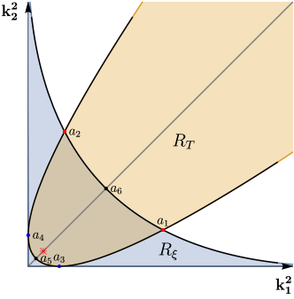
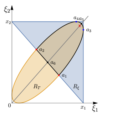
Figure 2: (left) The region of integration for variables $\bm{k}_{1T}^{2}$ and $\bm{k}_{2T}^{2}$ in the TMD factorization formulas (5.3) and (5.3). (right) The region of values of parameters $\xi_{1,2}$ (113) covered during the integration over $\bm{k}_{1T}^{2}$ and $\bm{k}_{2T}^{2}$. The points $a_{i}$ at both plots corresponds to the same values of $\bm{k}_{1T}^{2}$ and $\bm{k}_{2T}^{2}$.

The values collinear momentum-fractions of TMDPDFs are not fixed in the summed formula (5.3), but integrated in a particular range. It could be anticipated apriory, because the reparametrization invariance modifies the value of $x$’s (106), and thus any fixed choice is not frame-invariant. The $\delta$-functions express $\xi$’s as

$$\xi_{1} = \frac{x_{1}}{2}\left(1+\frac{\bm{k}_{1T}^{2}}{\tau^{2}}-\frac{\bm{k}_{2T}^{2}}{\tau^{2}}+\frac{\sqrt{\lambda(\bm{k}_{1T}^{2},\bm{k}_{2T}^{2},\tau^{2})}}{\tau^{2}}\right),$$ (116)

$$\xi_{2} = \frac{x_{2}}{2}\left(1-\frac{\bm{k}_{1T}^{2}}{\tau^{2}}+\frac{\bm{k}_{2T}^{2}}{\tau^{2}}+\frac{\sqrt{\lambda(\bm{k}_{1T}^{2},\bm{k}_{2T}^{2},\tau^{2})}}{\tau^{2}}\right),$$

where $\tau^{2}=2q^{+}q^{-}=Q^{2}+\bm{q}_{T}^{2}$, and $\lambda(a,b,c)=a^{2}+b^{2}+c^{2}-2ab-2ac-2bc$ is the kinematic function. The values of $\xi_{1,2}$ are restricted $0<\xi_{1,2}<1$ (due to the support properties of TMDPDF), which constraints the integration region of $\bm{k}_{1T}^{2}$ and $\bm{k}_{2T}^{2}$ to

$$R_{\xi}:\qquad 0<\bm{k}_{1T}^{2}<\tau^{2},\qquad 0<\bm{k}_{2T}^{2}<\tau+\bm{k}_{1T}^{2}-2\sqrt{\bm{k}_{1T}^{2}\tau^{2}}.$$ (117)

The region $R_{\xi}$ is shown in the fig.2(left) by blue color. The variables $\xi$ (116) can be seen as a kind-of-Nachmann variables Nachtmann:1973mr ; Georgi:1976ve for the TMD factorization theorem, which correct for the convolution integral for non-zero transverse momenta of partons.

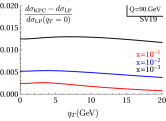
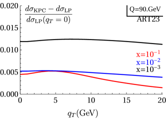
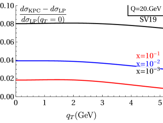
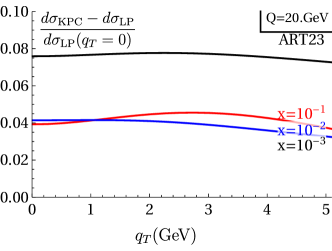
Figure 3: The difference of KPC-summed and LP cross-sections relative to the $q_{T}=0$ LP cross-section for the Drell-Yan reaction at different $q_{T}$ and different $x$. The plot in left(right) panels are based on SV19 Scimemi:2019cmh (ART23 Moos:2023yfa ) extraction of TMDPDF. Upper row is for $Q=90$GeV, and lower row is for $Q=20$GeV. Lines of different color corresponds to different values of $x$ (at $y=0$).

In full the integration region for (5.3) is $R_{\xi}\cap R_{T}$. It is compact. The maximum values of $\bm{k}_{T}^{2}$ are $(\sqrt{\tau^{2}}+\sqrt{\bm{q}_{T}^{2}})^{2}/4$ ($=Q^{2}/4$ at $\bm{q}_{T}^{2}=0$) which are reached at the points $a_{1,2}$ in fig.2. The arguments $\xi_{1,2}$ belongs to the region shown in fig.2(right). This region does not include the LP values of collinear momentum-fraction $x_{1,2}$ (113), but it includes the values $\sqrt{Q^{2}/s}e^{\pm y}$, which are often used in the phenomenology and is shown by the red star in fig.2.

In figs. 3 and 4, the comparison of KPC-summed (5.3) and LP (5.3) cross-sections is shown. For the comparison the extractions SV19 Scimemi:2019cmh (presented in the left panels) and ART23 Moos:2023yfa (presented in the right panels) were used. The perturbative orders are the same as used in the extractions. They are N³LL for SV19, and N⁴LL for ART23. The evolution of distributions is performed in the position space, then the TMDPDFs are Fourier-transformed and substituted into (5.3, 5.3). The results for different extraction have generally the same size but somewhat different behavior at $x>10^{-2}$.

The inclusion of KPCs results into an almost flat increase of the cross-section as a function of $q_{T}$, see fig.3. The size of the shift grows at smaller $x$’s and $Q$. In other words, the inclusion of KPCs does not significantly modify the shape of the LP prediction, but significantly changes the normalization. At the typical kinematic of the LHC (aka Z-boson production) the size of corrections is of the order of $1$%. It grows to $\sim 30-40$% at $Q\sim 10$GeV. Using the presented curves one can estimate the effective size of KPCs. Their order of magnitude is approximately described by

$$\frac{d\sigma|_{\text{KPC}}}{d\sigma|_{\text{LP}}}\sim 1+\frac{(2\text{GeV})^{2}}{x^{0.4}Q^{2}}.$$ (118)

This approximation is obtained by a two-parameter fit of SV19 and ART23 curves.

It is interesting to mention that the modern TMD phenomenology faces problems with the description of normalization of cross-section, while perfectly describes the shape. For LHC energies the issue is of order of few percents, while for low-energy fix-target data ($Q\sim 5-20$GeV) is tenths of percents Bertone:2019nxa ; Bacchetta:2019sam ; Vladimirov:2019bfa . The situation is worse for $Q\sim 2-4$GeV which are typical for Semi-Inclusive Deep-Inelastic Scattering (SIDIS). In this case the problem with normalization is of order of factor 2-3 Bacchetta:2022awv . Therefore, one could hope that inclusion of KPCs into the phenomenology will resolve this important problem.

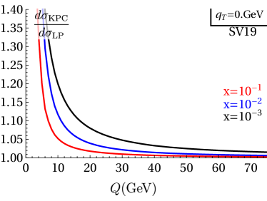
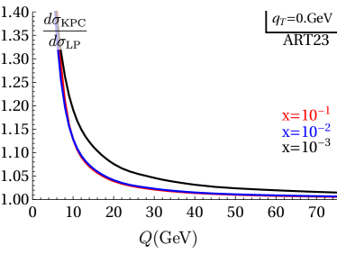
Figure 4: The ratio of KPC-summed to LP cross-sections for the Drell-Yan reaction at $q_{T}=0$ at different $Q$ and different $x$. The plot in left(right) panel is based on SV19 Scimemi:2019cmh (ART23 Moos:2023yfa ) extraction of TMDPDF. Lines of different color corresponds to different values of $x$ (at $y=0$).

6 Conclusion

The power corrections in the TMD factorization theorem provide a rich field for investigation. As described in the introduction, there are four conceptual types of power corrections: $q_{T}/Q$, $k_{T}/Q$, $\Lambda/Q$, and target-mass corrections. These corrections have distinct origins and characteristics. Importantly, different power corrections are significant in different kinematic regimes, which justifies considering them independently. In this work, I have derived the series of kinematic power corrections (KPCs) or $k_{T}/Q$-corrections that follow the leading power (LP) term. These corrections play a special role for the factorization theorem and are essential for its consistency because KPCs are responsible for restoring electromagnetic (EM) gauge invariance (charge conservation) and frame invariance, which are broken by the LP approximation. In that sense, the series of KPCs is the entailed part of the LP factorization theorem.

The KPCs that follow the LP term possess a distinctive mark: they only involve TMD distributions of twist-two. This feature allows for their straightforward extraction from the generic power expansion of operators. The resulting series is presented in equation (53). This series is summed in a simple expression (4.2), which is the main result of the work. The computation is done for the Drell-Yan process but can be generalized for other processes without conceptual problems.

One of the most significant features of KPCs is that they must obey the factorization theorem, even if other types of power corrections may violate it. This statement follows from the fact that KPCs are responsible for restoring the fundamental properties of the LP term, namely charge conservation and frame invariance. Consequently, the coefficient function for KPCs remains identical to the LP coefficient function. In sec. 3.3, I have explicitly verified this statement at the next-to-leading order (NLO) and demonstrated the restoration of the argument of the LP coefficient function to $q^{2}$. The latter is a non-trivial result as it indicates the impossibility of a strict power expansion beyond NLP.

The final formula for the cross-section is almost trivial – it tells that the cross-section can be computed with free massless quarks similar to a naive parton picture. However, with the present derivation, it attains a different status. It obeys the factorization theorem, and it is clear which part of the power expansion is included and which is neglected. The excluded terms consist of TMD distributions of twist-three and higher, as well as powers of $q_{T}/Q$

It is important to note that the derivation of the series of KPCs is contingent upon the definition of TMD-twist and higher twist distributions. The current derivation is based on the approach outlined in ref. Vladimirov:2021hdn , which leads to a consistent result. However, if an alternative definition is proposed, the series of KPCs could differ. In such a case, some of the present higher twist terms would be absorbed into the KPC series. In particular, the difference in the treatment of higher twist terms may describe the discrepancy between the present computation and ref. Balitsky:2020jzt .

Incorporating KPCs into TMD phenomenology is essential, as they play a crucial role in restoring the consistency of the formalism. Moreover, all perturbative ingredients remain unchanged since KPCs adhere to the LP factorization theorem. Therefore, including KPCs in phenomenological studies can be done without encountering conceptual difficulties while maintaining the achieved level of accuracy (currently at the N⁴LL order Moos:2023yfa ). The summed formula is valid in the same kinematic range of application as ordinary TMD factorization. Estimations made in sec. 5.3 demonstrate that including KPCs results in an almost constant increment of the cross-section. The magnitude of this correction depends on $Q$ and $x$. For typical LHC kinematics, the correction is around 1%, while at $Q\sim 4-5$ GeV, the correction can reach 100%. Interestingly, the deficiency in normalization for the TMD factorization at low energies has been reported by multiple groups. One could expect that these problems will be resolved with the inclusion of KPCs.

- (1) R. Angeles-Martinez et al., Transverse Momentum Dependent (TMD) parton distribution functions: status and prospects, Acta Phys. Polon. B 46 (2015) 2501 [1507.05267].
- (2) R. Boussarie et al., TMD Handbook, 2304.03302.
- (3) A. Vladimirov, Pion-induced Drell-Yan processes within TMD factorization, JHEP 10 (2019) 090 [1907.10356].
- (4) M. Bury, A. Prokudin and A. Vladimirov, Extraction of the Sivers function from SIDIS, Drell-Yan, and boson production data with TMD evolution, JHEP 05 (2021) 151 [2103.03270].
- (5) A. Bacchetta, V. Bertone, C. Bissolotti, G. Bozzi, M. Cerutti, F. Piacenza et al., Unpolarized Transverse Momentum Distributions from a global fit of Drell-Yan and Semi-Inclusive Deep-Inelastic Scattering data, 2206.07598.
- (6) R. Abdul Khalek et al., Science Requirements and Detector Concepts for the Electron-Ion Collider: EIC Yellow Report, 2103.05419.
- (7) A. Accardi et al., Strong Interaction Physics at the Luminosity Frontier with 22 GeV Electrons at Jefferson Lab, 2306.09360.
- (8) J.C. Collins, D.E. Soper and G.F. Sterman, Transverse Momentum Distribution in Drell-Yan Pair and W and Z Boson Production, Nucl. Phys. B 250 (1985) 199.
- (9) J. Collins, Foundations of perturbative QCD, vol. 32, Cambridge University Press (11, 2013).
- (10) T. Becher and M. Neubert, Drell-Yan Production at Small , Transverse Parton Distributions and the Collinear Anomaly, Eur. Phys. J. C 71 (2011) 1665 [1007.4005].
- (11) M.G. Echevarria, A. Idilbi and I. Scimemi, Factorization Theorem For Drell-Yan At Low And Transverse Momentum Distributions On-The-Light-Cone, JHEP 07 (2012) 002 [1111.4996].
- (12) S.M. Aybat and T.C. Rogers, TMD Parton Distribution and Fragmentation Functions with QCD Evolution, Phys. Rev. D 83 (2011) 114042 [1101.5057].
- (13) J.-Y. Chiu, A. Jain, D. Neill and I.Z. Rothstein, A Formalism for the Systematic Treatment of Rapidity Logarithms in Quantum Field Theory, JHEP 05 (2012) 084 [1202.0814].
- (14) I. Scimemi and A. Vladimirov, Systematic analysis of double-scale evolution, JHEP 08 (2018) 003 [1803.11089].
- (15) P.J. Mulders and R.D. Tangerman, The Complete tree level result up to order 1/Q for polarized deep inelastic leptoproduction, Nucl. Phys. B 461 (1996) 197 [hep-ph/9510301].
- (16) A. Bacchetta, M. Diehl, K. Goeke, A. Metz, P.J. Mulders and M. Schlegel, Semi-inclusive deep inelastic scattering at small transverse momentum, JHEP 02 (2007) 093 [hep-ph/0611265].
- (17) S. Arnold, A. Metz and M. Schlegel, Dilepton production from polarized hadron hadron collisions, Phys. Rev. D 79 (2009) 034005 [0809.2262].
- (18) I. Balitsky and A. Tarasov, Power corrections to TMD factorization for Z-boson production, JHEP 05 (2018) 150 [1712.09389].
- (19) I. Balitsky, Gauge-invariant TMD factorization for Drell-Yan hadronic tensor at small x, JHEP 05 (2021) 046 [2012.01588].
- (20) M. Inglis-Whalen, M. Luke, J. Roy and A. Spourdalakis, Factorization of power corrections in the Drell-Yan process in EFT, Phys. Rev. D 104 (2021) 076018 [2105.09277].
- (21) I. Balitsky, Drell-Yan angular lepton distributions at small x from TMD factorization., JHEP 09 (2021) 022 [2105.13391].
- (22) A. Vladimirov, V. Moos and I. Scimemi, Transverse momentum dependent operator expansion at next-to-leading power, 2109.09771.
- (23) M.A. Ebert, A. Gao and I.W. Stewart, Factorization for Azimuthal Asymmetries in SIDIS at Next-to-Leading Power, 2112.07680.
- (24) S. Rodini and A. Vladimirov, Factorization for quasi-TMD distributions of sub-leading power, 2211.04494.
- (25) S. Rodini and A. Vladimirov, Transverse momentum dependent factorization for SIDIS at next-to-leading power, 2306.09495.
- (26) S. Rodini and A. Vladimirov, Definition and evolution of transverse momentum dependent distribution of twist-three, JHEP 08 (2022) 031 [2204.03856].
- (27) R.A. Brandt and G. Preparata, Operator product expansions near the light cone, Nucl. Phys. B 27 (1971) 541.
- (28) D.J. Gross and S.B. Treiman, Light cone structure of current commutators in the gluon quark model, Phys. Rev. D 4 (1971) 1059.
- (29) V. Moos and A. Vladimirov, Calculation of transverse momentum dependent distributions beyond the leading power, JHEP 12 (2020) 145 [2008.01744].
- (30) W. Rarita and J. Schwinger, On a theory of particles with half integral spin, Phys. Rev. 60 (1941) 61.
- (31) E.G. Delgado Acosta, V.M. Banda Guzmán and M. Kirchbach, Bosonic and fermionic Weinberg-Joos (j,0) (0,j) states of arbitrary spins as Lorentz tensors or tensor-spinors and second-order theory, Eur. Phys. J. A 51 (2015) 35 [1503.07230].
- (32) B. Geyer, M. Lazar and D. Robaschik, Decomposition of nonlocal light cone operators into harmonic operators of definite twist, Nucl. Phys. B 559 (1999) 339 [hep-th/9901090].
- (33) R.L. Jaffe and X.-D. Ji, Chiral odd parton distributions and polarized Drell-Yan, Phys. Rev. Lett. 67 (1991) 552.
- (34) A.V. Belitsky, X. Ji and F. Yuan, Final state interactions and gauge invariant parton distributions, Nucl. Phys. B 656 (2003) 165 [hep-ph/0208038].
- (35) R.L. Jaffe, Spin, twist and hadron structure in deep inelastic processes, in Ettore Majorana International School of Nucleon Structure: 1st Course: The Spin Structure of the Nucleon, pp. 42–129, 1, 1996 [hep-ph/9602236].
- (36) I.I. Balitsky and V.M. Braun, Evolution Equations for QCD String Operators, Nucl. Phys. B 311 (1989) 541.
- (37) A.V. Belitsky and D. Mueller, Twist- three effects in two photon processes, Nucl. Phys. B 589 (2000) 611 [hep-ph/0007031].
- (38) L. Gamberg, Z.-B. Kang, D.Y. Shao, J. Terry and F. Zhao, Transverse-momentum-dependent factorization at next-to-leading power, 2211.13209.
- (39) S. Wandzura and F. Wilczek, Sum Rules for Spin Dependent Electroproduction: Test of Relativistic Constituent Quarks, Phys. Lett. B 72 (1977) 195.
- (40) V.M. Braun and A.N. Manashov, Operator product expansion in QCD in off-forward kinematics: Separation of kinematic and dynamical contributions, JHEP 01 (2012) 085 [1111.6765].
- (41) V.M. Braun and A.N. Manashov, Kinematic power corrections in off-forward hard reactions, Phys. Rev. Lett. 107 (2011) 202001 [1108.2394].
- (42) J.C. Collins and D.E. Soper, Back-To-Back Jets in QCD, Nucl. Phys. B 193 (1981) 381.
- (43) A.A. Vladimirov, Self-contained definition of the Collins-Soper kernel, Phys. Rev. Lett. 125 (2020) 192002 [2003.02288].
- (44) M.A. Ebert and F.J. Tackmann, Resummation of Transverse Momentum Distributions in Distribution Space, JHEP 02 (2017) 110 [1611.08610].
- (45) D. Boer, P.J. Mulders and F. Pijlman, Universality of T odd effects in single spin and azimuthal asymmetries, Nucl. Phys. B 667 (2003) 201 [hep-ph/0303034].
- (46) S. Bhattacharya, A. Metz, V.K. Ojha, J.-Y. Tsai and J. Zhou, Exclusive double quarkonium production and generalized TMDs of gluons, Phys. Lett. B 833 (2022) 137383 [1802.10550].
- (47) M.G. Echevarria, P.A. Gutierrez Garcia and I. Scimemi, GTMDs and the factorization of exclusive double Drell-Yan, Phys. Lett. B 840 (2023) 137881 [2208.00021].
- (48) V.M. Braun, A.N. Manashov, D. Mueller and B. Pirnay, Resolving kinematic ambiguities in QCD predictions for Deeply Virtual Compton Scattering, PoS DIS2014 (2014) 225 [1407.0815].
- (49) A.V. Manohar and I.W. Stewart, The Zero-Bin and Mode Factorization in Quantum Field Theory, Phys. Rev. D 76 (2007) 074002 [hep-ph/0605001].
- (50) A. Vladimirov, Structure of rapidity divergences in multi-parton scattering soft factors, JHEP 04 (2018) 045 [1707.07606].
- (51) I. Balitsky, Rapidity-only TMD factorization at one loop, JHEP 03 (2023) 029 [2301.01717].
- (52) V.M. Braun, A.N. Manashov and J. Rohrwild, Renormalization of Twist-Four Operators in QCD, Nucl. Phys. B 826 (2010) 235 [0908.1684].
- (53) A.V. Manohar, Deep inelastic scattering as x — 1 using soft collinear effective theory, Phys. Rev. D 68 (2003) 114019 [hep-ph/0309176].
- (54) R.N. Lee, A. von Manteuffel, R.M. Schabinger, A.V. Smirnov, V.A. Smirnov and M. Steinhauser, Quark and Gluon Form Factors in Four-Loop QCD, Phys. Rev. Lett. 128 (2022) 212002 [2202.04660].
- (55) I. Moult, H.X. Zhu and Y.J. Zhu, The four loop QCD rapidity anomalous dimension, JHEP 08 (2022) 280 [2205.02249].
- (56) I. Scimemi, A. Tarasov and A. Vladimirov, Collinear matching for Sivers function at next-to-leading order, JHEP 05 (2019) 125 [1901.04519].
- (57) V.M. Braun, Y. Ji and A. Vladimirov, QCD factorization for twist-three axial-vector parton quasidistributions, JHEP 05 (2021) 086 [2103.12105].
- (58) V. Shtabovenko, R. Mertig and F. Orellana, FeynCalc 9.3: New features and improvements, Comput. Phys. Commun. 256 (2020) 107478 [2001.04407].
- (59) J. Collins, CSS Equation, etc, Follow from Structure of TMD Factorization, 1212.5974.
- (60) M.G. Echevarría, A. Idilbi and I. Scimemi, Soft and Collinear Factorization and Transverse Momentum Dependent Parton Distribution Functions, Phys. Lett. B 726 (2013) 795 [1211.1947].
- (61) M. Beneke, T. Feldmann and D. Seidel, Systematic approach to exclusive , decays, Nucl. Phys. B 612 (2001) 25 [hep-ph/0106067].
- (62) M. Beneke and M. Neubert, QCD factorization for B — PP and B — PV decays, Nucl. Phys. B 675 (2003) 333 [hep-ph/0308039].
- (63) I.I. Balitsky, V.M. Braun and A.V. Kolesnichenko, Power corrections 1 / Q**2 to parton sum rules for deep inelastic scattering from polarized targets, Phys. Lett. B 242 (1990) 245 [hep-ph/9310316].
- (64) A.V. Belitsky and D. Mueller, Resummation of target mass corrections in two photon processes: Twist two sector, Phys. Lett. B 507 (2001) 173 [hep-ph/0102224].
- (65) A.V. Belitsky and D. Mueller, Exclusive electroproduction revisited: treating kinematical effects, Phys. Rev. D 82 (2010) 074010 [1005.5209].
- (66) V.M. Braun, A.N. Manashov, D. Müller and B.M. Pirnay, Deeply Virtual Compton Scattering to the twist-four accuracy: Impact of finite- and target mass corrections, Phys. Rev. D 89 (2014) 074022 [1401.7621].
- (67) M.E. Luke and A.V. Manohar, Reparametrization invariance constraints on heavy particle effective field theories, Phys. Lett. B 286 (1992) 348 [hep-ph/9205228].
- (68) A.V. Manohar, T. Mehen, D. Pirjol and I.W. Stewart, Reparameterization invariance for collinear operators, Phys. Lett. B 539 (2002) 59 [hep-ph/0204229].
- (69) C. Marcantonini and I.W. Stewart, Reparameterization Invariant Collinear Operators, Phys. Rev. D 79 (2009) 065028 [0809.1093].
- (70) I. Scimemi and A. Vladimirov, Analysis of vector boson production within TMD factorization, Eur. Phys. J. C 78 (2018) 89 [1706.01473].
- (71) I. Scimemi and A. Vladimirov, Non-perturbative structure of semi-inclusive deep-inelastic and Drell-Yan scattering at small transverse momentum, JHEP 06 (2020) 137 [1912.06532].
- (72) V. Moos, I. Scimemi, A. Vladimirov and P. Zurita, Extraction of unpolarized transverse momentum distributions from fit of Drell-Yan data at N4LL, 2305.07473.
- (73) O. Nachtmann, Positivity constraints for anomalous dimensions, Nucl. Phys. B 63 (1973) 237.
- (74) H. Georgi and H.D. Politzer, Freedom at Moderate Energies: Masses in Color Dynamics, Phys. Rev. D 14 (1976) 1829.
- (75) V. Bertone, I. Scimemi and A. Vladimirov, Extraction of unpolarized quark transverse momentum dependent parton distributions from Drell-Yan/Z-boson production, JHEP 06 (2019) 028 [1902.08474].
- (76) A. Bacchetta, V. Bertone, C. Bissolotti, G. Bozzi, F. Delcarro, F. Piacenza et al., Transverse-momentum-dependent parton distributions up to N3LL from Drell-Yan data, JHEP 07 (2020) 117 [1912.07550].