Unraveling the role of interactions in non-equilibrium transformations

Abstract

For arbitrary non-equilibrium transformations in complex systems, we show that the distance between the current state and a target state can be decomposed into two terms: one corresponding to an independent estimate of the distance, and another corresponding to interactions, quantified using the relative mutual information between the variables. This decomposition is a special case of a more general decomposition involving successive orders of correlation or interactions among the system’s degrees of freedom. To illustrate its practical significance, we study the thermalization of two optically trapped colloidal particles with hydrodynamic coupling. Our results show that, increasing pairwise interaction strength enhances the separation between the time-dependent non-equilibrium state and the final state, prolonging the non-equilibrium state’s longevity. In more general setups, where it is possible to control the strength of different orders of interactions, our findings offer a way to disentangle their effects on the transformation process.

A broad range of microscopic non-equilibrium processes are time-dependent, where the state of the system, described in terms of probability distributions, changes as a function of time. Examples include the thermalization of systems prepared in an arbitrary initial state [1], self-assembly of biological molecules [2, 3, 4], protein folding [5, 6], several single-molecule experiments [7, 8], and microscopic devices that are time-dependently controlled [9, 10, 11]. In all these cases, the trajectory of the system progresses through a series of states, influenced by interactions among the different degrees of freedom of the system, with the environment, and external controls/feedbacks [12, 13].

Several recent studies have tried to identify governing principles for such processes in terms of the distance between the initial and final states of the system, the time taken for the transformation, and the associated thermodynamic costs. These include the refinements of the Second Law [14, 15, 16, 17], optimal connections [18, 19, 20], speed limits [21, 22, 23, 24] as well as their trade-offs with the entropic costs [25, 26, 27, 23, 28]. However, the fundamental effects of interactions among the different degrees of freedom of the system, on the distance or time taken for non-equilibrium transformations are relatively less understood.

In a recent development, Refs. [29, 30] made significant progress in this direction. They demonstrated that in systems with multiple degrees of freedom and having multi-partite dynamics, the estimate of irreversibility in a non-equilibrium steady state can be decomposed into contributions from individual variables, and a series of non-negative contributions from correlations among variable pairs, triplets, and higher-order combinations. Their proof is based on representing irreversibility as a Kullback-Leibler divergence, which measures the relative likelihood of trajectories over their time-reversed counterparts.

In general, the Kullback-Leibler divergence quantifies the distance between any two probability distributions, and it has recently gained renewed interest in studying non-equilibrium transformations and control of microscopic systems [31, 32, 17]. In certain cases, it also provides estimates of the thermodynamic cost of the process [33, 34, 12]. Hence, understanding how this distance function depends on interactions is crucial, as it enables the optimization of processes based on interactions, and the design of more efficient and reliable non-equilibrium controls.

Here we address this problem by implementing a non-trivial decomposition of the Kullback-Leibler divergence. This decomposition primarily consists of two terms: one corresponding to an independent estimate of the distance, representing hypothetical marginal processes which are non-interacting, and another corresponding to interactions, quantified using the relative mutual information between the variables. This decomposition is further shown to arise from a previously known decomposition of the joint distribution involving successive orders of correlation or interactions among the system’s degrees of freedom [35, 36, 37]. Crucially this decomposition is not limited to multi-partite systems. Applying the decomposition to an interacting pair of colloids that undergoes thermalization, we find that increasing the strength of pairwise interactions generically increases the distance between the current state and the target state, prolonging the longevity of the non-equilibrium initial state. In more general setups, where it is possible to control the strength of different orders of interactions, our results provide means to separate out their effects on the transformation process.

We begin by considering a system whose state is described using the variable ${\bm{x}}_{t}\in\mathbb{R}^{N}$, and probability distribution $P({\bm{x}}_{t})$. We have dropped the explicit dependence on $t$ for simplicity of notation. Note that one of the elements of vector ${\bm{x}}_{t}$ can also be an external control or a feedback protocol. Let us now consider a scenario where the probability distribution $P({\bm{x}}_{t})$ dynamically evolves from an initial distribution $P_{i}({\bm{x}}_{t_{i}})$ to a final / target distribution $P_{f}({\bm{x}}_{t_{f}})$ in a time-dependent manner. At any given time $t$, the distance of the instantaneous distribution $P({\bm{x}}_{t})$ to the target distribution can be computed in terms of the Kullback-Leibler (KL) divergence between the two distributions as [38],

$$\begin{split}D_{\rm KL}(P({\bm{x}}_{t})||P_{f}({\bm{x}}_{t}))&=\int_{{\bm{x}}_{t}}P({\bm{x}}_{t})\log\frac{P({\bm{x}}_{t})}{P_{f}({\bm{x}}_{t})}.\end{split}$$ (1)

Next, assume we know the marginal distributions, $P_{m}^{i}(x_{t}^{i})=\int_{{\bm{x}}_{-i}}P({\bm{x}}_{t})$, where ${\bm{x}}_{-i}$ corresponds to all variables except $x_{t}^{i}$. One can obtain an independent distance in terms of these marginals as,

$$\begin{split}D^{i}_{\rm{Ind}}=\int_{x_{t}^{i}}P_{m}^{i}(x_{t}^{i})\log\frac{P_{m}^{i}(x_{t}^{i})}{P_{f,m}^{i}(x_{t}^{i})}.\end{split}$$ (2)

The sum of the independent distances over all variables, $D_{\rm Ind.}=\sum_{i}D^{i}_{\rm{Ind}}$, provides an estimate of the distance that one would have got if the variables were independently measured. By examining the difference $D-D_{\rm Ind.}$, we find,

$$\begin{split}D&-\sum_{i}D^{i}_{\rm{Ind}}\\ &=\int_{{\bm{x}}_{t}}P({\bm{x}}_{t})\left[\log\frac{P({\bm{x}}_{t})}{\prod_{i}P_{m}^{i}(x_{t}^{i})}-\log\frac{P_{f}({\bm{x}}_{t})}{\prod_{i}P_{m,f}^{i}(x_{t}^{i})}\right]\\ &=I({\bm{x}}_{t})-I_{f}^{\prime}({\bm{x}}_{t}),\end{split}$$ (3)

where $I({\bm{x}}_{t})$ is the mutual information of the current state, generalized to $N$ variables (also referred to as the total correlation [39]), and $I_{f}^{\prime}({\bm{x}}_{t})$ is the cross mutual information of the target state, where the average is computed with respect to the current state.

Eq. (3) is our first key observation: the distance between any two distributions can be decomposed into two terms: a term coming from the marginal probabilities and another coming from interactions between the local variables, i.e.,

$$D=D_{\rm Ind.}+D_{\rm Int.},$$ (4)

where $D_{\rm Int.}\equiv I({\bm{x}}_{t})-I_{f}^{\prime}({\bm{x}}_{t})$, appears as the relative mutual information between the current state and the target state. Note that the sign of this interaction term could be positive or negative, depending on the choice of the final distribution and the nature of interactions. Eq. (3) also has a simple information theoretic interpretation: Interactions contribute to the distance only if the mutual information of the current state differs from the cross mutual information of the target state. This means, there could be instances where accurate distance measurements can be solely obtained from the marginal statistics, even when the local variables are correlated.

Interestingly, using a known decomposition of the joint probability distribution, one can show that the total distance further breaks down into contributions from interactions among subsets of $k<N$ variables. This decomposition is due to the generalized Kirkwood superposition approximation [35, 37, 40, 41, 36], which is traditionally used in the context of sampling of equilibrium distributions. We briefly describe it in the following: Assume that we know all the $(N-1)^{\rm th}$ order marginal distributions,

$$P_{N-1}(x_{1},\dots x_{N-1})=\int_{{\bm{x}_{t}}^{-[N-1]}}P({\bm{x}}_{t}),$$ (5)

where the integration is done over the variable that is not in the subset $\{x_{1},\dots x_{N-1}\}$. The Kirkwood superposition approximation provides an estimate to the joint probability distribution $\hat{P}_{N-1}({\bm{x}}_{t})\simeq P({\bm{x}}_{t})$ in terms of these marginals, as [35, 37],

$$\log\hat{P}_{N-1}({\bm{x}}_{t})=\sum_{\alpha=1}^{N-1}(-1)^{N-\alpha+1}\log\prod_{j=1}^{C^{N}_{\alpha}}P_{\alpha}^{j},$$ (6)

where the product is over all marginal densities $P_{\alpha}^{j}$ obtained for a subset of variables of size $\alpha\leq N-1$. By successively applying the Kirkwood approximation to the RHS of Eq. (6), we can get an estimate of the joint distribution $P({\bm{x}}_{t})$ in terms of marginals of any order $k<N$. We refer to the resulting $k-$th order approximation as $\hat{P}_{k}({\bm{x}}_{t})$. In particular, for $k=1$, we will arrive at the product of single-variable marginals [41, 36].

Using these distributions, we can obtain an estimate of the distance that is accurate to $k$-th order interactions, as,

$$D^{(k)}=\int_{{\bm{x}}_{t}}P({\bm{x}}_{t})\log\frac{\hat{P}_{k}({\bm{x}}_{t})}{\hat{P}_{f,k}({\bm{x}}_{t})}.$$ (7)

Due to the expansion in Eq. (6), $D^{(k)}$ is fully determined in terms of marginal probabilities upto order $k$. For $k=1$, we recover $D^{(1)}=D_{\rm Ind.}$. We can also safely define $D^{(N)}\equiv D$. It is then natural to compare $D^{(k)}$ with $D^{(k-1)}$. If $D^{(k)}=D^{(k-1)}$, it implies that the $k$th-order dynamics is redundant, as it does not contribute to the total distance. However, if that is not the case, then the $k$th-order dynamics contribute, and we can separate the contribution as,

$$D^{(k)}_{\rm Int.}=D^{(k)}-D^{(k-1)}.$$ (8)

This yields the full decomposition of the total distance into interactions of different orders as,

$$D=D^{(1)}_{\rm Int.}+D^{(2)}_{\rm Int.}+D^{(3)}_{\rm Int.}\cdots+D^{(N)}_{\rm Int.}.$$ (9)

Note that the decomposition above is similar in spirit to the decomposition of irreversibility in Refs. [29, 30], breaking down the distance between two distributions into contributions from individual elements in the system, interactions between pairs of elements, interactions among triplets, and so on. However, the derivation of Eq. (9) does not assume multi-partite dynamics. Additionally, individual terms in the expansion, $D^{(k)}$, can be negative. In practice, $D^{(k)}$ can be computed from the knowledge of the full joint distribution or empirically obtained distributions, where only a collection of $k$ variables are measured simultaneously.

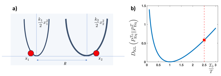
Figure 1: a) Schematics of two identical, hydrodynamically coupled colloidal particles in two spatially separated quadratic potential wells of stiffness $k_{1}$ and $k_{2}$. b) The distance between the initial equilibrium system at temperature $T_{0}$ and the final equilibrium system at temperature $T$. The figures made in this paper correspond to the particular parameter choice $T_{0}/T=2.5$, which is marked in red. The other parameter choices are: $k_{1}=1;\;k_{2}=2;\;\gamma=1;\;\eta=1;\;k_{B}=1.$

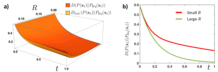
Figure 2: a) The total distance function $D\equiv D_{\rm KL}\left(P({\bm{x}}_{t})||P_{\rm Eq}({\bm{x}}_{t})\right)$ as well as the independent distance $D_{\rm Ind.}$ for different values of $R$ and $t$, for fixed values of initial and final temperatures as well as other model parameters. We find that $D>D_{\rm Ind.}$ for all values of $R$ and $t$. b) The total distance function $D\equiv D_{\rm KL}\left(P({\bm{x}}_{t})||P_{\rm Eq}({\bm{x}}_{t})\right)$ for two values of the separation $R$ ($R=0.1$ and $R=0.5$) between the two optical traps. We find that the system at small separation takes longer to thermalize.

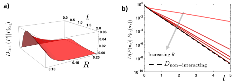
Figure 3: a) The interaction distance $D_{\rm Int.}$ for different values of time $t$ and separation $R$. We find that as we decrease $R$ and bring the two particles closer to each other, the interaction distance $D_{\rm Int.}$ increases. b) The total distance $D$ compared with the distance computed for the non-interacting case $D_{\rm non-interacting}\equiv\lim_{R\rightarrow\infty}D$, for different values of $R$. As expected, we find that $D_{\rm non-interacting}\leq D$ for all values of $R$ and $t$, saturating the bound in the $R\rightarrow\infty$ limit.

To demonstrate the usefulness of the decomposition, we consider the problem of thermalization of two identical, hydrodynamically coupled colloidal particles in two spatially separated quadratic potential wells, as shown in Fig. 1. These colloidal particles are prepared in an equilibrium state at temperature $T_{0}$ and then let to thermalize in an aqueous solution at temperature $T$. This model has been extensively studied both theoretically [42, 43, 44] and experimentally [45, 46]. The dynamics is governed by the Langevin equations:

$$\begin{split}\dot{x}(t)&=H_{11}(-k_{1}x+f_{1}(t))+H_{12}(-k_{2}y+f_{2}(t))\\ \dot{y}(t)&=H_{21}(-k_{1}x+f_{1}(t))+H_{22}(-k_{2}y+f_{2}(t)),\end{split}$$ (10)

where $x(t)$ and $y(t)$ represents the positions of these particles at different times. The parameters $k_{1}$ and $k_{2}$ denote the optical stiffness of the two traps. The constants $H_{11}=H_{22}=1/(6\pi\eta a)=1/\gamma$   and   $H_{12}=H_{21}=1/(4\pi\eta R)$, where $R$ is the center - center distance between the two traps and $a$ is the radius of the particle, are the lowest order components, in $1/R$, of the Oseen Tensor [47] for motions in the longitudinal directions. Here $\gamma$ is the viscous drag coefficient. The value of $R$ determines the interaction between the colloidal particles. As $R\to\infty$, the interaction between the colloidal particles vanishes and our system turns to a non-interacting system. The terms $f_{1}(t)$ and $f_{2}(t)$ are the random Brownian forces which are delta correlated in time.

Given that the system is initially prepared in a state different from its thermal equilibrium state in the new environment, it exists in a non-equilibrium state characterized by a certain distance from its eventual thermal state. Quantifying this distance in terms of Kullback-Leibler divergence has gained significant interest in recent times, primarily in the context of non-trivial thermalization behaviours such as Mpemba effects [48, 49, 50, 34, 51] or the study of asymmetries of thermal relaxation [52, 53, 54, 55, 56]. In these cases, $D_{\rm KL}\left(P({\bm{x}}_{t})||P_{\rm Eq}({\bm{x}}_{t})\right)$ is also the same as the excess free energy of the state $P({\bm{x}}_{t})$ which vanishes as the system equilibrates (see Refs. [52, 34] for a simple derivation).

For the model we consider, leveraging the fact that it is a linear system of stochastic differential equations, it is possible to analytically compute the instantaneous probability distribution $P({\bm{x}}_{t})$ in terms of all the parameters in the system, for any value of time $t$ (See Appendix A). Using these solutions, it can be verified that the variables $x$ and $y$ are anti-correlated for any $t>0$. The strength of correlations increases when $R$ decreases. Further, at equilibrium (in the $t\rightarrow 0$ and $t\rightarrow\infty$ limit), the correlations vanish.

Using the exact solutions for the distributions, we can further compute the distance function $D_{\rm KL}\left(P({\bm{x}}_{t})||P_{\rm Eq}({\bm{x}}_{t})\right)$. In particular, when $t=0$, we get the distance between the initial equilibrium system at temperature $T_{0}$ and the final equilibrium system at temperature $T$, which can be used to compare initial states and pick the equivalent ones that are equidistant [52, 53, 54, 56] from the final thermal state. For our model, this initial distance function is found to only depend on the ratio $T_{0}/T$ and is given by,

$$D_{\rm KL}\left(P^{T_{0}}_{\rm Eq}({\bm{x}})||P_{\rm Eq}^{T}({\bm{x}})\right)=-1+\frac{T_{0}}{T}+\log\frac{T}{T_{0}}.$$ (11)

Thus, if we consider an ensemble of systems with different values of $R$, a fixed initial temperature, and an ambient temperature, all of them will have the same distance to the final thermal state at $t=0$. For a particular choice of parameters, we show this initial distance function in Fig. 1b. The rest of the plots in this paper correspond to the point $T_{0}/T=2.5$ in this curve, which has the initial distance $D_{\rm KL}\left(P^{T_{0}}_{\rm Eq}({\bm{x}})||P_{\rm Eq}^{T}({\bm{x}})\right)=0.5837$.

For arbitrary times, the distance functions $D_{\rm KL}\left(P({\bm{x}}_{t})||P_{\rm Eq}^{T}({\bm{x}}_{t})\right)$ will in general depend on the the parameter $R$. Furthermore, using explicit analytical solutions of $P({\bm{x}}_{t})$ and its marginals, we can separately compute the independent distance, interaction distance as well as the distance function in the non-interacting limit of $R\rightarrow\infty$. Since our system consists of only two interacting particles, the decomposition in Eq. (9) only has two terms, namely $D^{(1)}_{\rm Int.}=D_{\rm Ind.}$ and $D^{(2)}_{\rm Int.}=D_{\rm Int.}=D-D_{\rm Ind.}$, given by,

$$D_{\rm Int.}=\scalebox{1.0}{$\int_{x_{t},y_{t}}P(x_{t},y_{t})\log\frac{P(x_{t},y_{t})P_{{\rm Eq},m}(x_{t})P_{{\rm Eq},m}(y_{t})}{P_{\rm Eq}(x_{t},y_{t})P_{m}(x_{t})P_{m}(y_{t})}$}$$ (12)

In Figure 2, we present our central findings. Figure 2a illustrates the plots of $D$ and $D_{\rm Ind.}$ for various values of $R$ and $t$, while keeping other model parameters fixed. At $t=0$, all states are equidistant from the final thermal state, as expected. We also find that $D_{\rm Int.}=0$ for any fixed value of $R$, even though the variables are correlated in the initial and final distributions. This means the initial distance function can entirely be determined by the marginal statistics of $x$ and $y$. However, for $t>0$, and any value of $R$ we observe that $D>D_{\rm Ind.}$, which means interactions positively contribute to the total distance. Specifically, when the two traps are brought closer, the value of $D$ increases for all $t$. Refer to Figure 2b for a demonstration of this behavior with two different values of $R$.

In Figure 3a, we plot the interaction distance $D_{\rm Int.}$ for varying time $t$ and different values of $R$. As $R$ decreases, the interaction distance contribution $D_{\rm Int.}$ increases. Finally, in Figure 3b, we compare the total distance $D$ with the distance computed for the non-interacting case, denoted as $D_{\rm non-interacting}\equiv\lim_{R\rightarrow\infty}D$. We observe that $D_{\rm non-interacting}\leq D$ for all values of $R$ and $t$. Moreover, this bound saturates in the limit $R\rightarrow\infty$.

In summary, we have shown that, in arbitrary non-equilibrium transformations, the distance between the current state and a target state can be decomposed into two terms: one corresponding to an independent estimate of the distance, representing hypothetical marginal processes which are non-interacting, and another corresponding to interactions, quantified using the relative mutual information between the variables. The interaction term can further be decomposed into contributions from interactions between pairs of elements, interactions among triplets, and so on. The results are demonstrated by considering the example of the thermalization of two optically trapped colloidal particles that are hydrodynamically coupled. In this case, increasing the pairwise interaction strength is found to enhance the separation between the time-dependent non-equilibrium state and the final state, thereby increasing the longevity of the non-equilibrium initial state.

Our results suggest that harnessing local interactions could have applications in controlling and manipulating systems towards desired states. In setups where it is possible to control the strength of different orders of interactions, our findings offer a way to disentangle their effects on the transformation process, and to identify the ones that can assist the transformation. Further research could delve into specific applications in non-equilibrium control problems [32, 57, 58, 59, 19] where understanding these effects could be valuable, or resource theories [60], where maintaining non-equilibrium states for extended periods could be beneficial.

Acknowledgements.- Nordita is partially supported by Nordforsk. MR and SKM thank the Kerala Theoretical Physics Initiative - Active Research Training (KTPI - ART) program for facilitating the research collaboration. SKM acknowledges the Knut and Alice Wallenberg Foundation for financial support through Grant No. KAW 2021.0328. SKM thanks the members of the Soft-Matter Group, NORDITA, Stockholm, Sweden, for helpful discussions on Refs. [30, 29]. SKM thanks Biswajit Das and Shuvojit Paul, Light Matter Lab, IISER Kolkata, India for helpful discussions on the model studied.

Appendix A Exact calculation for the system of interacting colloids

Here, we describe the calculation of the distance functions for the model of interacting colloids. We follow the notations in Ref. [61]. To begin with, we rewrite Eq. (10) as a matrix equation,

$$\dot{{\bm{r}}}(t)=-{\bm{A}}{\bm{r}}(t)+{\bm{\epsilon}}(t)$$ (13)

with $\langle{\bm{\epsilon}}(t){\bm{\epsilon}}(s)\rangle=2{\bm{D}}\delta(t-s)$ where

$$\begin{split}{\bm{r}}(t)&=\begin{bmatrix}x(t)\\ y(t)\end{bmatrix},\\ {\bm{A}}&=\begin{bmatrix}\frac{k_{1}}{\gamma}&\frac{k_{2}}{4\pi\eta R}\\ \frac{k_{1}}{4\pi\eta R}&\frac{k_{2}}{\gamma}\end{bmatrix},\\ {\bm{D}}&=\left[\begin{array}[]{cc}\frac{k_{B}T}{\gamma}&\frac{k_{B}T}{4\pi\eta R}\\ \frac{k_{B}T}{4\pi\eta R}&\frac{k_{B}T}{\gamma}\\ \end{array}\right],\\ {\bm{\eta}}(t)&=\begin{bmatrix}\epsilon_{1}(t)\\ \epsilon_{2}(t)\end{bmatrix}.\end{split}$$ (14)

Now to find the probability distribution of the system at any time, first, we write a Fokker - Planck equation equivalent to our Langevin equation as

$$\frac{\partial P(t,{\bm{r}}|t_{0},{\bm{r}}_{0})}{\partial t}=\sum_{i,j}(\frac{\partial}{\partial r_{i}}[A_{ij}r_{j}+D_{ij}\frac{\partial}{\partial r_{j}}]P(t,{\bm{r}}|t_{0},{\bm{r}}_{0}))\;,\\$$ (15)

where $P(t,{\bm{r}}|t_{0},{\bm{r}}_{0})$ is the conditional probability that the system is in a position ${\bm{r}}$ at time $t$, given that it was at ${\bm{r}}_{0}$ at time $t_{0}$.

The Fokker - Planck equation (15) is exactly solvable, and the solution is found to be

$$P(t,{\bm{r}}|t_{0},{\bm{r}}_{0})=\scalebox{0.9}{{\hbox{\frac{e^{-\frac{1}{2} [ {\bm{r}} - e^{-(t-t_{0}){\bm{A}}}{\bm{r}}_{0}]^{T}\; {\bm{\Sigma}}^{-1}(t-t_{0}) \;[{\bm{r}} - e^{-(t-t_{0}){\bm{A}}}{\bm{r}}_{0}]}}{\sqrt{(2 \pi)^{2}\; \det\;{\bm{\Sigma}}(t-t_{0})}}}}}\;,$$ (16)

where the covariance matrix is

$${\bm{\Sigma}}(t)={\bm{\Sigma}}(\infty)-e^{-t{\bm{A}}}\;{\bm{\Sigma}}(\infty)\;e^{-t{\bm{A}}^{T}}\;,$$ (17)

and ${\bm{\Sigma}}(\infty)$ is found by solving the below matrix equation

$${\bm{A}}{\bm{\Sigma}}(\infty)+{\bm{\Sigma}}(\infty){\bm{A}}^{T}=2{\bm{D}}\\$$ (18)

If the matrix ${\bm{A}}$ is positive definite, it is guaranteed that the system will reach a stationary Gaussian distribution at $t\rightarrow\infty$, which will have the covariance matrix ${\bm{\Sigma}}^{-1}(\infty)$. For our model, we obtain,

$${\bm{\Sigma}}(\infty)=\left(\begin{array}[]{cc}\frac{k_{B}T}{k_{1}}&0\\ 0&\frac{k_{B}T}{k_{2}}\end{array}\right).$$ (21)

In terms of this matrix, we can obtain the equilibrium distribution of the system as,

$$P_{\rm Eq}({\bm{x}})=\frac{1}{\sqrt{(2\pi)^{2}\det{\bm{\Sigma}}(\infty)}}e^{-\frac{1}{2}{\bm{x}}{\bm{\Sigma}}^{-1}(\infty){\bm{x}}}.$$ (22)

Note that this distribution explicitly depends on the temperature $T$. When we set $T=T_{0}$, we get the equilibrium distribution at temperature $T_{0}$. Furthermore, the time-dependent distribution corresponding to the thermal relaxation from a distribution at an initial temperature $T_{0}$ to an ambient temperature $T$ can be obtained by performing the integration,

$$P({\bm{x}}_{t})=\int_{{\bm{x}}_{0}}P_{\rm Eq}^{T_{0}}({\bm{x}}_{0})P(t,{\bm{x}}_{t}|t_{0},{\bm{x}}_{0})$$ (23)

where $P(t,{\bm{x}}_{t}|t_{0},{\bm{x}}_{0})$ is given by Eq. (16). The results in this manuscript are obtained by first explicitly evaluating this integral to get $P({\bm{x}}_{t})$ and computing the relevant distance functions in terms of that.

References

- Dattagupta [2012] S. Dattagupta, Relaxation phenomena in condensed matter physics (Elsevier, 2012).
- Whitesides and Grzybowski [2002] G. M. Whitesides and B. Grzybowski, Self-assembly at all scales, Science 295, 2418 (2002).
- Pollard and Borisy [2003] T. D. Pollard and G. G. Borisy, Cellular Motility Driven by Assembly and Disassembly of Actin Filaments, Cell 112, 453 (2003).
- Mauro et al. [2014] M. Mauro, A. Aliprandi, D. Septiadi, N. S. Kehr, and L. De Cola, When self-assembly meets biology: luminescent platinum complexes for imaging applications, Chemical Society Reviews 43, 4144 (2014).
- Dobson [2003] C. M. Dobson, Protein folding and misfolding, Nature 426, 884 (2003).
- Creighton [1990] T. E. Creighton, Protein folding., Biochemical journal 270, 1 (1990).
- Ritort [2006] F. Ritort, Single-molecule experiments in biological physics: methods and applications, Journal of Physics: Condensed Matter 18, R531 (2006).
- Ciliberto [2017] S. Ciliberto, Experiments in stochastic thermodynamics: Short history and perspectives, Physical Review X 7, 021051 (2017).
- Pop [2010] E. Pop, Energy dissipation and transport in nanoscale devices, Nano Research 3, 147 (2010).
- Bergfield and Ratner [2013] J. P. Bergfield and M. A. Ratner, Forty years of molecular electronics: Non-equilibrium heat and charge transport at the nanoscale, physica status solidi (b) 250, 2249 (2013).
- Martínez et al. [2016] I. A. Martínez, É. Roldán, L. Dinis, D. Petrov, J. M. Parrondo, and R. A. Rica, Brownian carnot engine, Nature physics 12, 67 (2016).
- Sagawa and Ueda [2012] T. Sagawa and M. Ueda, Fluctuation theorem with information exchange: Role of correlations in stochastic thermodynamics, Physical review letters 109, 180602 (2012).
- Barato and Seifert [2014] A. Barato and U. Seifert, Unifying three perspectives on information processing in stochastic thermodynamics, Physical review letters 112, 090601 (2014).
- Aurell et al. [2012] E. Aurell, K. Gawedzki, C. Mejia-Monasterio, R. Mohayaee, and P. Muratore-Ginanneschi, Refined second law of thermodynamics for fast random processes, Journal of statistical physics 147, 487 (2012).
- Deffner and Lutz [2010] S. Deffner and E. Lutz, Generalized clausius inequality for nonequilibrium quantum processes, Phys. Rev. Lett. 105, 170402 (2010).
- Kim [2021] E.-j. Kim, Information geometry, fluctuations, non-equilibrium thermodynamics, and geodesics in complex systems, Entropy 23, 1393 (2021).
- Nakazato and Ito [2021] M. Nakazato and S. Ito, Geometrical aspects of entropy production in stochastic thermodynamics based on wasserstein distance, Physical Review Research 3, 043093 (2021).
- Ito [2023] S. Ito, Geometric thermodynamics for the fokker–planck equation: stochastic thermodynamic links between information geometry and optimal transport, Information Geometry , 1 (2023).
- Chennakesavalu and Rotskoff [2023] S. Chennakesavalu and G. M. Rotskoff, Unified, geometric framework for nonequilibrium protocol optimization, Physical Review Letters 130, 107101 (2023).
- Rotskoff and Crooks [2015] G. M. Rotskoff and G. E. Crooks, Optimal control in nonequilibrium systems: Dynamic riemannian geometry of the ising model, Physical Review E 92, 060102 (2015).
- Shiraishi et al. [2018] N. Shiraishi, K. Funo, and K. Saito, Speed limit for classical stochastic processes, Physical review letters 121, 070601 (2018).
- Van Vu and Saito [2023a] T. Van Vu and K. Saito, Topological speed limit, Physical review letters 130, 010402 (2023a).
- Yoshimura and Ito [2021] K. Yoshimura and S. Ito, Thermodynamic uncertainty relation and thermodynamic speed limit in deterministic chemical reaction networks, Physical review letters 127, 160601 (2021).
- Funo et al. [2019] K. Funo, N. Shiraishi, and K. Saito, Speed limit for open quantum systems, New Journal of Physics 21, 013006 (2019).
- Lee et al. [2022] J. S. Lee, S. Lee, H. Kwon, and H. Park, Speed limit for a highly irreversible process and tight finite-time landauer’s bound, Physical review letters 129, 120603 (2022).
- Falasco and Esposito [2020] G. Falasco and M. Esposito, Dissipation-time uncertainty relation, Physical Review Letters 125, 120604 (2020).
- Van Vu and Saito [2023b] T. Van Vu and K. Saito, Thermodynamic unification of optimal transport: Thermodynamic uncertainty relation, minimum dissipation, and thermodynamic speed limits, Physical Review X 13, 011013 (2023b).
- Kuznets-Speck and Limmer [2021] B. Kuznets-Speck and D. T. Limmer, Dissipation bounds the amplification of transition rates far from equilibrium, Proceedings of the National Academy of Sciences 118, e2020863118 (2021).
- Lynn et al. [2022a] C. W. Lynn, C. M. Holmes, W. Bialek, and D. J. Schwab, Decomposing the local arrow of time in interacting systems, Phys. Rev. Lett. 129, 118101 (2022a).
- Lynn et al. [2022b] C. W. Lynn, C. M. Holmes, W. Bialek, and D. J. Schwab, Emergence of local irreversibility in complex interacting systems, Physical Review E 106, 034102 (2022b).
- Ito [2018] S. Ito, Stochastic thermodynamic interpretation of information geometry, Physical review letters 121, 030605 (2018).
- Aurell et al. [2011] E. Aurell, C. Mejía-Monasterio, and P. Muratore-Ginanneschi, Optimal protocols and optimal transport in stochastic thermodynamics, Physical review letters 106, 250601 (2011).
- Shiraishi and Saito [2019] N. Shiraishi and K. Saito, Information-theoretical bound of the irreversibility in thermal relaxation processes, Physical review letters 123, 110603 (2019).
- Chétrite et al. [2021] R. Chétrite, A. Kumar, and J. Bechhoefer, The metastable mpemba effect corresponds to a non-monotonic temperature dependence of extractable work, arXiv preprint arXiv:2101.06394 (2021).
- McClendon et al. [2012] C. L. McClendon, L. Hua, G. Barreiro, and M. P. Jacobson, Comparing conformational ensembles using the kullback–leibler divergence expansion, Journal of chemical theory and computation 8, 2115 (2012).
- Galas et al. [2017] D. J. Galas, G. Dewey, J. Kunert-Graf, and N. A. Sakhanenko, Expansion of the kullback-leibler divergence, and a new class of information metrics, Axioms 6, 8 (2017).
- Tritchler et al. [2011] D. L. Tritchler, L. Sucheston, P. Chanda, and M. Ramanathan, Information metrics in genetic epidemiology, Statistical applications in genetics and molecular biology 10 (2011).
- Lu and Raz [2017] Z. Lu and O. Raz, Nonequilibrium thermodynamics of the markovian mpemba effect and its inverse, Proceedings of the National Academy of Sciences 114, 5083 (2017).
- Watanabe [1960] S. Watanabe, Information theoretical analysis of multivariate correlation, IBM Journal of research and development 4, 66 (1960).
- Somani et al. [2009] S. Somani, B. J. Killian, and M. K. Gilson, Sampling conformations in high dimensions using low-dimensional distribution functions, The Journal of chemical physics 130 (2009).
- Killian et al. [2007] B. J. Killian, J. Yundenfreund Kravitz, and M. K. Gilson, Extraction of configurational entropy from molecular simulations via an expansion approximation, The Journal of chemical physics 127 (2007).
- Hough and Ou-Yang [2002] L. Hough and H. Ou-Yang, Correlated motions of two hydrodynamically coupled particles confined in separate quadratic potential wells, Physical Review E 65, 021906 (2002).
- Kotar et al. [2010] J. Kotar, M. Leoni, B. Bassetti, M. C. Lagomarsino, and P. Cicuta, Hydrodynamic synchronization of colloidal oscillators, Proceedings of the National Academy of Sciences 107, 7669 (2010).
- Reichert and Stark [2004] M. Reichert and H. Stark, Hydrodynamic coupling of two rotating spheres trapped in harmonic potentials, Physical Review E 69, 031407 (2004).
- Paul et al. [2018] S. Paul, R. Kumar, and A. Banerjee, Two-point active microrheology in a viscous medium exploiting a motional resonance excited in dual-trap optical tweezers, Physical Review E 97, 042606 (2018).
- Paul et al. [2017] S. Paul, A. Laskar, R. Singh, B. Roy, R. Adhikari, and A. Banerjee, Direct verification of the fluctuation-dissipation relation in viscously coupled oscillators, Physical Review E 96, 050102 (2017).
- Doi and Edwards [1988] M. Doi and S. F. Edwards, The theory of polymer dynamics, Vol. 73 (oxford university press, 1988).
- Kumar and Bechhoefer [2020] A. Kumar and J. Bechhoefer, Exponentially faster cooling in a colloidal system, Nature 584, 64 (2020).
- Bechhoefer et al. [2021] J. Bechhoefer, A. Kumar, and R. Chétrite, A fresh understanding of the mpemba effect, Nature Reviews Physics , 1 (2021).
- Biswas and Rajesh [2023] A. Biswas and R. Rajesh, Mpemba effect for a brownian particle trapped in a single well potential, arXiv preprint arXiv:2305.06613 (2023).
- Degünther and Seifert [2022] J. Degünther and U. Seifert, Anomalous relaxation from a non-equilibrium steady state: An isothermal analog of the mpemba effect, Europhysics Letters 139, 41002 (2022).
- Lapolla and Godec [2020] A. Lapolla and A. c. v. Godec, Faster uphill relaxation in thermodynamically equidistant temperature quenches, Phys. Rev. Lett. 125, 110602 (2020).
- Manikandan [2021] S. K. Manikandan, Equidistant quenches in few-level quantum systems, Phys. Rev. Res. 3, 043108 (2021).
- Van Vu and Hasegawa [2021] T. Van Vu and Y. Hasegawa, Toward relaxation asymmetry: Heating is faster than cooling, Physical Review Research 3, 043160 (2021).
- Dieball et al. [2023] C. Dieball, G. Wellecke, and A. Godec, Asymmetric thermal relaxation in driven systems: Rotations go opposite ways, arXiv preprint arXiv:2304.06702 (2023).
- Meibohm et al. [2021] J. Meibohm, D. Forastiere, T. Adeleke-Larodo, and K. Proesmans, Relaxation-speed crossover in anharmonic potentials, Physical Review E 104, L032105 (2021).
- Yan et al. [2022] J. Yan, H. Touchette, G. M. Rotskoff, et al., Learning nonequilibrium control forces to characterize dynamical phase transitions, Physical Review E 105, 024115 (2022).
- Rotskoff et al. [2017] G. M. Rotskoff, G. E. Crooks, and E. Vanden-Eijnden, Geometric approach to optimal nonequilibrium control: Minimizing dissipation in nanomagnetic spin systems, Physical Review E 95, 012148 (2017).
- Abreu and Seifert [2012] D. Abreu and U. Seifert, Thermodynamics of genuine nonequilibrium states under feedback control, Physical review letters 108, 030601 (2012).
- Gour et al. [2015] G. Gour, M. P. Müller, V. Narasimhachar, R. W. Spekkens, and N. Y. Halpern, The resource theory of informational nonequilibrium in thermodynamics, Physics Reports 583, 1 (2015).
- Argun et al. [2017] A. Argun, J. Soni, L. Dabelow, S. Bo, G. Pesce, R. Eichhorn, and G. Volpe, Experimental realization of a minimal microscopic heat engine, Phys. Rev. E 96, 052106 (2017).