Collective epithelial migration is mediated by the unbinding of hexatic defects

Abstract

Collective cell migration in epithelia relies on cell intercalation: i.e. a local remodelling of the cellular network that allows neighbouring cells to swap their positions. While in common with foams and other passive cellular fluids, intercalation in epithelia crucially depends on active processes, where the local geometry of the network and the contractile forces generated therein conspire to produce an “avalanche” of remodelling events, which collectively give rise to a vortical flow at the mesoscopic length scale. In this article we formulate a continuum theory of the mechanism driving this process, built upon recent advances towards understanding the hexatic (i.e. $6-$fold ordered) structure of epithelial layers. Using a combination of active hydrodynamics and cell-resolved numerical simulations, we demonstrate that cell intercalation takes place via the unbinding of topological defects, naturally initiated by fluctuations and whose late-times dynamics is governed by the interplay between passive attractive forces and active self-propulsion. Our approach sheds light on the structure of the cellular forces driving collective migration in epithelia and provides an explanation of the observed extensile activity of in vitro epithelial layers.

From humble soap froths [1, 2, 3] down to epithelial layers [4, 5, 6, 7, 8, 9, 10], confluent cellular fluids use intercalation to flow, even in the absence of gaps and interstitial structures. At the heart of this locomotion strategy is a mechanism known as topological rearrangement process of the first kind – or T1 for brevity – through which the vertices of a honeycomb network merge and then split, thereby leading to a remodelling of the network’s topology. An isolated T1, however, is not sufficient to achieve a full intercalation. To illustrate this concept, let us focus on the group of four cells depicted in Fig. 1 and hereafter referred to as primary cell cluster. A T1 occurs when the internal $3-$fold coordinated vertices shrink until merging into a $4-$fold vertex, and then split along the orthogonal direction. Such an internal T1, however, leaves the number and, importantly, the positions of external vertices of each cell unchanged. Thus, despite this concept having received little attention in the literature (see, e.g., Refs. [11, 12, 10, 13, 14, 15]), it is impossible to achieve collective migration by means of isolated T1 processes. To make progress, here we introduce the notion of T1 avalanche: i.e. a series of T1 processes involving the external vertices of the primary cluster. A full cell intercalation then consists of an internal T1, followed by a T1 avalanche, and is schematically summarized in Fig. 1a. Crucially, internal T1 processes do not always trigger a T1 avalanche and eventually a full intercalation. After the first T1, where the internal $3-$fold vertices shrink to a $4-$fold vertex, the cluster may reverse its dynamics and return to its original configuration (see Fig. 1b). In the following, we refer to this scenario as T1 cycle: i.e. a direct T1 followed by an inverse T1, which does not permanently alter the configuration of the honeycomb network. Intuitively, and as we show next, whether the initial T1 triggers an avalanche, hence collective migration, or a cycle, is determined by the configuration of contractile stresses exerted by the cells, which, in turn, are modulated by the local geometry of the primary cluster.

In order to develop a continuum mechanical description of the aforementioned mechanism, here we leverage on recent advances toward deciphering orientational order in epithelial layers [16, 17, 18, 19, 20, 21, 22]. The latter originates from the cells’ anisotropic shape and results in the emergence of liquid crystal phases collectively known as $p-$atics, with $p$ an integer reflecting the symmetry of the system under rotation by $2\pi/p$. The honeycomb structure of epithelial layers, in particular, has been shown to give rise to hexatic order (i.e. $p=6$) at length scales ranging from one to dozens of cells, depending on the cells’ density and molecular repertoire, as well as the mechanical properties of the substrate [19, 20, 21].

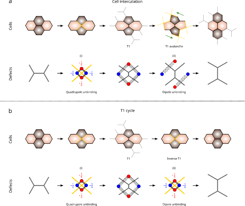
Figure 1: Cell intercalation and T1 cycle. (a) A full cell intercalation, consists of a T1, which remodels the internal vertex structure of the primary quadrupole and a T1 avalanche. The latter reconfigures the external vertices, thereby triggering new T1 processes across the neighboring cells. In the language of topological defects, the T1 translates to the (i) unbinding of a $\pm 1/6$ defect quadrupole and (ii) T1 avalanche to a further unbinding of the quadrupole into a pair of dipoles. (b) In a T1 cycle, the primary cell cluster undergoes a T1, followed by an inverse T1, which restores its initial configuration. The process corresponds to (i) the unbinding of a defect quadrupole and (ii) its annihilation.

Now, in the language of continuum mechanics, the cell-wide morphological transformations underlying T1 processes can be described in terms of topological defects known as disclinations: i.e. point-like singularities in the otherwise regular configuration of a continuous $p-$atic order parameter – i.e. $\Psi_{p}=\langle e^{ip\vartheta}\rangle$, with $\vartheta$ the orientation of the individual building blocks and $\langle\cdots\rangle$ the ensemble average [23, 24] – around which the average cellular orientation rotates by $2\pi s$, with $s=\pm 1/p,\,\pm 2/p\ldots$ the winding number or “strength” of the defect. Disclinations are a hallmark of passive and active liquid crystals alike and, in the realm of multicellular systems, are believed to facilitate a number of biomechanical functions, such as the development of protrusions in the morphogenesis of Hydra [25, 26], the extrusion of apoptotic cells [27], or the onset of directed motion under confinement [28]. In passive two-dimensional matter, disclinations mediate the transition from solid to liquid via a process known as Kosterlitz-Thouless-Halperin-Nelson-Young (KTHNY) melting scenario [29, 30, 31, 32, 33]. According to this, the hierarchical unbinding of neutral defect complexes – i.e. for which $\sum_{i}s_{i}=0$ – renders the system progressively more disordered. Our working hypothesis is that the competition between active and passive forces drives a similar unbinding mechanism in epithelial layers. In the following, we clarify the various steps and possible outcomes of this process and test this hypothesis against both hydrodynamic and cell-resolved numerical simulations.

As a starting point, we focus on the intermediate configuration of primary cell cluster comprising two orthogonal pairs of pentagonal and heptagonal cells, as shown in the central column of Fig. 1. This configuration, which corresponds to the most elementary short-ranged excitation of a honeycomb network, can be described in the language of topological defects as a quadrupole of $\pm 1/6$ disclinations. As in two-dimensional melting, such a defect-structure can arise spontaneously, as consequence of spatiotemporal fluctuations of physical or biological nature. The two complementary remodelling events following the intermediate configuration, i.e. the T1 avalanche (Fig. 1a) and cycle (Fig. 1b), correspond instead to the two possible “fates” of this initial excitation. Upon unbinding [Figs. 1a-(i) and 1b-(i)], the four defects comprising the quadrupole can further unbind into two $\pm 1/6$ disclination dipoles [Fig. 1a-(ii)], or annihilate [Fig. 1b-(ii)], thereby restoring the initial defect-free configuration. As we demonstrate next, the former scenario corresponds to the T1 avalanche and the latter to the T1 cycle. To this end, we identify three geometrical requirements that a model of cell intercalation must fulfill, regardless of the desired level of biophysical accuracy. 1) The average orientation of the cells must rotate by $\pi/6$ with respect to initial configuration. 2) Both in the primary clusters and its surrounding cells, must perform a local convergent extension: i.e. move inward in one direction, and outward along the orthogonal one (see e.g. Refs. [34, 35, 36, 37]). We stress that the adjective local, is used here to distinguish this process from convergent extension as intended in developmental biology, where the same rearrangement occurs at the scale of the entire organism. 3) In order to remodel the external vertices and initiate a T1 avalanche, the primary cluster must undergo a spontaneous shear deformation.

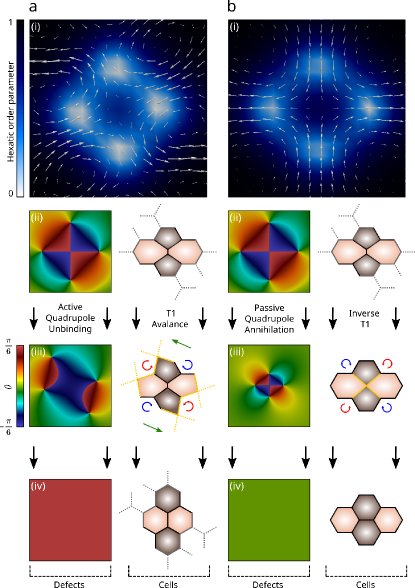
Figure 2: T1 avalanche and cycle as defect unbinding and annihilation. (a) T1 avalanche. (i) Backflow velocity field generated during the unbinding of an active, hexatic defect quadrupole. The three panels below show the orientation field associated with (ii) the quadruple in the initial configuration, (iii) as it unbinds in a pair of $\pm 1/6$ dipoles and (iv) after the dipoles have move outside of the region of interest, together with the corresponding configuration of the primary cluster. As the dipoles move away from each other, the cells surrounding the primary cluster rotate clockwise (blue) and counterclockwise (red). (b) T1 cycle. (i)-(iv) Analogous sequence as in panel (a), but associated with the annihilation of the defect quadrupole. Notice that, in panel (iii), the direction of the flow is reversed.

In the following, we show that our construction not only fulfills these requirements, but, harnessing the predictive power of active hydrodynamics, provides readily testable experimental predictions. To this end, we numerically integrate the hydrodynamic equations of active hexatic liquid crystals, introduced by Armengol-Collado et al. in Ref. [20] (see Methods). To follow the fate of a T1, we assume the cells to be initially horizontally oriented, so that the phase $\theta$ of the hexatic order parameter, $\Psi_{6}=|\Psi_{6}|e^{6i\theta}$, is $\theta=0$, and construct a configuration featuring a quadrupole of $\pm 1/6$ disclinations [see Figs. 2a-(i) and 2b-(i)]. Along one full loop encircling each of these defects, $\theta$ changes by $\pm\pi/3$, with the sign reflecting that of the defect’s winding number. Since the external boundary of the primary cluster consists of four half loops, this implies that $\theta$ varies in the range $-\pi/6\leq\theta\leq\pi/6$ around the quadruple, as indicated by the alternating blue and red tones in Fig. 2a-(ii) and 2b-(ii). Once the defect quadrupole breaks into two dipoles, this new orientation propagates from the boundary of the primary cluster into space between the dipoles [see Fig. 2a-(iii)], while leaving the orientation of the cells in the exterior essentially undistorted. Thus, the unbinding of a $\pm 1/6$ defect quadrupole from a defect-free configuration and its break up into two dipoles drives a $\pi/6$ rotation of the cells between the dipoles [see Fig. 2a-(iv)], consistently with our first requirement. Conversely, if defects annihilate [see Fig. 2b-(iii)], the cells’ initial orientation is restored after a transient orientational fluctuation [see Fig. 2b-(iv)].

In order to address the second and third requirements, we look at the configuration of the velocity field $\bm{v}$, corresponding to the average velocity of the cells in the surrounding of the primary cluster. As well documented in the theoretical [38, 39, 40] and experimental [27, 41, 42, 43, 28] literature of active nematic liquid crystals, the distortion induced by topological defects drives a flow, whose structure and direction is determined by the defect’s strength and the magnitude of the active stresses collectively exerted by the cells. Immediately after unbinding, an approximated expression for the velocity of the flow caused by the defect quadrupole can be analytically calculated. Calling $\bm{r}=|\bm{r}|(\cos\phi\,\bm{e}_{x}+\sin\phi\,\bm{e}_{y})$ the distance from the center of the primary cluster and $\ell$ the cluster’s size, this is given by

$$\bm{v}\approx\frac{120\alpha_{6}\ell^{4}}{\eta}\left[\left(4-6\log{\frac{\bm{|r|}}{\ell}}-3\,\frac{\bm{|r|}^{2}}{\ell^{2}}\right)\cos 6\phi\right]\frac{\bm{r}}{|\bm{r}|^{8}}\;.$$ (1)

where $\alpha_{6}$ a constant, with dimensions of force over volume, embodying the active stresses exerted by the cells and modulated by the local hexatic order, and $\eta$ the shear viscosity (see Methods for details). Thus, in close proximity the primary cluster, where $|\bm{r}|/\ell\gtrapprox 1$, Eq. (1) gives $v_{x}(x,0)\sim\alpha_{6}/(\eta\ell^{4})\,x$ and $v_{y}(y,0)\sim-\alpha_{6}/(\eta\ell^{4})\,y$. In agreement with our second requirement, this is typical structure of a stagnation flow, whose realization at the cellular scale is a local convergent extension. We stress that, consistently with the cooperative and mesoscale nature of cell intercalation, Eq. (1) cannot be obtained from the mere superposition of the flows individually sourced by the defects, as a consequence of the non-linear dependance of the order parameter on the average cellular orientation. Finally, we notice that the specific direction of motion – i.e. the sign of $\bm{v}$ – depends solely on $\alpha_{6}$, which, in turn, is either positive or negative depending on whether the active stresses exerted within the cell layer are respectively contractile or extensile.

As the cellular layer starts remodelling and the defects comprising the quadrupole migrate away from their original position, a solution of the hydrodynamic equations becomes analytically inaccessible, but can be obtained from a numerical integration of the hydrodynamic equations and is displayed in Figs. 2a and 2b, for two different $\alpha_{6}$ values. When $\alpha_{6}$ is large and negative, the quadrupole splits into two $\pm 1/6$ dipoles moving away from each other at an angle of approximatively $5\pi/6$. Such a shear deformation is further enhanced by the coupling between hexatic order and flow, which, in a way not dissimilar to flow alignment effects in nematic liquid crystals, drives a rotation of the local orientation [44]. Such a flow-induced rotation, whose handedness depends upon the sign of a material parameter analogous to the flow alignment parameter of nematics, biases the unbinding dynamics of the defect dipoles, thereby setting, in concert with the passive Coulomb-like forces at play, the direction along which the dipoles move away from each other [45]. Finally, switching off active stresses – i.e. $\alpha_{6}=0$, shown in Fig. 2b – suppresses both defect unbinding and shear. Consistently, inverting the direction of active forces from extensile to contractile – i.e. $\alpha_{6}>0$, see Supplementary Information – results in a speed up of defects annihilation, hence of the T1 cycle, but never lead to the unbinding of $\pm 1/6$ pairs, thus to the onset of a T1 avalanche.

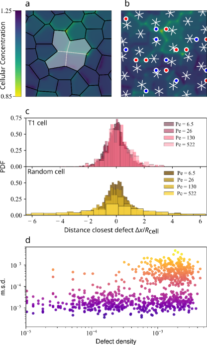
Figure 3: Collective cell migration as defect ubinding in the multiphase field model. (a) Example of a four-cell cluster as it undergoes a T1 process, together with (b) the reconstructed $6-$fold orientation field. The $6-$legged stars mark the local $6-$fold orientation of the cells (see Methods), while the red and blue dots denotes the $+1/6$ and $-1/6$ defects. (c) Probability distribution of finding a T1 (red tones) and a random cell (yellow tones) at a given distance from a defect, for four different values of the cells’ Péclet number ${\rm Pe}$. The data indicate a prominent correlation between T1 process and topological defects. (d) The mean square displacement (m.s.d) of cells versus defect density. We identify two distinct sub-populations of cells: “slow” (blue tones), with no correlation to the local density, and “fast” (yellow tones), located where the local defect density is higher. The former correspond to cells undergoing a T1 cycle and the latter participating to a T1 avalanche, hence to collective cell migration.

Having demonstrated the viability of our hydrodynamic approach, we next outline a number of general predictions, the most striking of which is that collective epithelial migration, as it results from cell intercalation, is a process of activity-guided defect unbinding. To this end, we perform numerical simulations of the multiphase field model of epithelia [46], which have been proved to capture various aspects of epithelial organization, including the recently found hexanemaitc multiscale order [19, 20, 21]. The results of these simulations are summarized in Fig. 3. In order to demonstrate the correlation between collective migration and topological defects, we investigate different regimes, distinguished by the cells’ Péclet number ${\rm Pe}=(v_{0}D_{r}^{-1})/R_{\rm cell}$ given by the ratio between the persistence length $v_{0}D_{r}^{-1}$ – where $v_{0}$ is the cells’ propulsion speed, $D_{r}^{-1}$ the persistence time of their trajectories – and $R_{\rm cell}$ the nominal cell radius (see Methods for details). In each regime, we reconstruct the probability of finding a T1 at a given distance from a defect (see Figs. 3a and 3b) and compare it with that of an arbitrary cell. Both distributions are approximatively Gaussian and have vanishing mean if expressed in terms of the signed distance $\Delta x$ (see Fig. 3c) or $\Delta y$. Furthermore, for small ${\rm Pe}$ values, where the short correlation time renders the system more disordered and dense of defects, the two probability distributions are hardly distinguishable, with the probability of finding a defect in proximity of a T1 only slightly larger than that associated with an arbitrary cell. As ${\rm Pe}$ is increased and the density of defects decreases, the latter probability distribution becomes flatter and flatter, while the former remains unchanged, thereby confirming that T1 processes are de facto a realization of hexatic defect unbinding. Finally, to correlate structure and dynamics we show, in Fig. 3d, the mean squared displacement of T1 cells versus the local defect density. Our data confirm the existence of two different classes: i.e. “slow” and “fast” cells, respectively denoted by blue and yellow tones. While for both classes of cells the mean squared displacement is roughly uniform for all values of the local defect density, fast cells only appear where the density is higher, thus providing an alternative signature of T1 cycles and avalanches. Cells undergoing a T1 cycle oscillate about their initial position, but do not participate to collective migration and exhibits, therefore, a small mean square displacement. By contrast cells involved in a T1 avalanche perform collective migration and, based on the correspondence here identified, can only be found in regions of high defect densities.

Before concluding, we discuss three especially striking aspects of collective cell migration highlighted by our approach and amenable to experimental scrutiny. First, from the active flow given by Eq. (1) and neglecting irrelevant inertial effects, one can estimate the magnitude of the active forces at play: i.e. $F_{\rm active}\sim\alpha_{6}/\ell^{-3}$. Such a scaling form results primarily from the $6-$fold structure of cellular forces under the assumption – still to be verified in hexatic epithelial layers, but consistent with previous observations on nematic cell cultures [47, 27, 41, 42, 28] – that $\alpha_{6}$ is, at least approximatively, spatially uniform. Second, in order for these forces to prompt defect unbinding, thereby triggering a T1 avalanche, they must overcome the passive Coulomb-like forces driving their annihilation. At the length scale of the primary cluster, the magnitude of the latter is roughly given by $F_{\rm passive}\sim L_{6}/\ell$, with $L_{6}$ the orientational stiffness of the hexatic phase (see Methods). Equating $F_{\rm active}$ and $F_{\rm passive}$ provides an estimate of the typical size of the primary cluster at which the cellular layer becomes unstable to collective migration: i.e. $\ell_{6}=\sqrt{|\alpha_{6}|/L_{6}}$. This active hexatic length scale was identified in Ref. [20] and is believed to play a role analog to that of the active nematic length scale $\ell_{2}=\sqrt{L_{2}/|\alpha_{2}|}$ [39]. The latter is the fundamental parameter controlling the collective behavior of active nematic liquid crystals and, depending on how it compares with other extrinsic and intrinsic length scales, determines the hydrodynamic stability [48] of active nematics, the distribution of the vortex area in chaotic cytoskeletal flows [49, 50], the size of nematic domains in bacterial colonies [51] and in vitro cultures of spindle-like cells [42] etc. Similarly, we expect that confining epithelia at length scales smaller than $\ell_{6}$ has the effect of suppressing cell intercalation and possibly render necessary different locomotion strategies and possibly favoring a switch to mesenchymal phenotypes. Lastly, in agreement with recent experimental evidence [27, 42, 43], our analysis shows that only an extensile activity can fuel collective migration in confluent epithelia and, leveraging on the familiar language of topological defects, it further provides a simple key to rationalizing the mechanical advantage of such a biological strategy: i.e. only extensile forces can provide the type of repulsive interactions that are necessary for defects to unbind, thus to trigger a T1 avalanche.

In conclusion, we have investigated the physical mechanisms behind cell intercalation in confluent epithelial layers, using a combination of continuum and discrete modelling. After having established that a isolated T1 processes are insufficient to achieve collective migration, we introduced the notion of T1 avalanche and demonstrated that this results from the unbinding of neutral quadrupoles of hexatic disclinations. As in the KTHNY melting scenario [31], the latter are spontaneously generated by fluctuations and can either annihilate, thereby restoring the original configuration, or further unbind in two pairs of $\pm 1/6$ disclinations, which, by moving away from each other, stir and shear the cellular network, thereby initiating other T1 processes, which, cooperatively, gives rise to cell migration. Our theory sheds light on the structure of the cellular forces driving collective migration in epithelia, suggests the possibility of a confinement-induced switch to mesenchymal phenotypes and provides an explanation of the observed extensile activity of in vitro epithelial layers [27, 42, 43].

Methods

Hydrodynamic equations of epithelial layers

Our hydrodynamic equations of epithelial layers have been given in Ref. [20] and account for both hexatic and nematic order, with the former being dominant at short and the latter at long length scales. Since cell intercalation occurs at small length scales, here we can ignore nematic order and focus solely on the hydrodynamics of the hexatic phase. In addition to the standard density $\rho$ and velocity $\bm{v}$, this can be described in terms of the $6-$fold order parameter tensor $\bm{Q}_{6}=4\left\llbracket\langle\bm{\nu}^{\otimes 6}\rangle\right\rrbracket=4|\Psi_{6}|\left\llbracket\bm{n}^{\otimes 6}\right\rrbracket$, where $\bm{\nu}=\cos\vartheta\,\bm{e}_{x}+\sin\vartheta\,\bm{e}_{y}$ and $\bm{n}=\cos\theta\,\bm{e}_{x}+\sin\theta\,\bm{e}_{y}$ are respectively the fluctuating and average orientation of the hexatic bulding blocks and the operator $\left\llbracket\cdots\right\rrbracket$ renders its argument traceless and symmetric (see Refs. [23, 24] for a general introduction to $p-$atic hydrodynamics). The short scale hydrodynamic equations of the epithelial layer are then given, in the most generic form, by

$$\frac{D\rho}{Dt}+\rho\nabla\cdot\bm{v}=(k_{\rm d}-k_{\rm a})\rho\;,$$ (2a)

$$\rho\,\frac{D\bm{v}}{Dt}=\nabla\cdot\bm{\sigma}+\bm{f}\;,$$ (2b)

$$\frac{D\bm{Q}_{6}}{Dt}=\Gamma_{6}\bm{H}_{6}+6\big{\llbracket}\bm{Q}_{6}\cdot\bm{\omega}\big{\rrbracket}+\lambda_{6}\big{\llbracket}\nabla^{\otimes 4}\bm{u}\big{\rrbracket}$$

$$+\bar{\lambda}_{6}\mbox{tr}(\bm{u})\bm{Q}_{6}+\nu_{6}\big{\llbracket}\bm{u}^{\otimes 3}\big{\rrbracket}\;.$$ (2c)

with $D/Dt=\partial_{t}+\bm{v}\cdot\nabla$ is the material derivative. In Eq. (2a), $k_{\rm d}$ and $k_{\rm a}$ the cell division and apoptosis rates, here assumed equal. For simplicity, we also assume uniform density throughout the system to that Eq. (2a) reduces to the standard incompressibility condition $\nabla\cdot\bm{v}=0$. In Eq. (2b) $\bm{\sigma}$ is the total stress tensor and $\bm{f}$ an external body force. In Eq. (2c), $\bm{u}=[\nabla\bm{v}+(\nabla\bm{v})^{\intercal}]/2$ and $\bm{\omega}=[\nabla\bm{v}-(\nabla\bm{v})^{\intercal}]/2$, with $\intercal$ indicating transposition, are respectively the strain rate and vorticity tensors and entail the coupling between hexatic order and flow, with $\lambda_{6}$ and $\nu_{6}$ material constants and $\left(\nabla^{\otimes n}\right)_{i_{1}i_{2}...i_{n}}=\partial_{i_{1}}\partial_{i_{2}}\ldots\,\partial_{i_{n}}$. Because of incompressibility, the term $\bar{\lambda}_{6}\mbox{tr}(\bm{u})\bm{Q}_{6}$ in Eq. (2c) vanishes. The tensor $\bm{H}_{6}=-\delta F/\delta\bm{Q}_{6}$ is the hexatic analog of the molecular tensor, dictating the relaxation dynamics of the order parameter tensor toward the minimum of the orientational free energy

$$F=\int{\rm d}A\,\left(\frac{L_{6}}{2}\,|\nabla\bm{Q}_{6}|^{2}+\frac{A_{6}}{2}\,|\bm{Q}_{6}|^{2}+\frac{B_{6}}{4}\,|\bm{Q}_{4}|^{4}\right)\;,$$ (3)

where $|\cdots|^{2}$ is the Euclidean norm and is such that $|\bm{Q}_{6}|^{2}=|\Psi_{6}|^{2}/2$. The constant $L_{6}$ is the order parameter stiffness, while $A_{6}$ and $B_{6}$ are phenomenological constants setting the magnitude of the coarse-grained complex order parameter at equilibrium: $|\Psi_{6}|=|\Psi_{6}^{(0)}|=\sqrt{-2A_{6}/B_{6}}$, when $H_{i_{1}i_{2}\cdots\,i_{6}}=0$.

The stress tensor figuring in Eq. (2b) can be customarily decomposed in a passive and an active contributions: i.e. $\bm{\sigma}=\bm{\sigma}^{({\rm p})}+\bm{\sigma}^{({\rm a})}$. The passive stress, in turn, can be expressed as $\bm{\sigma}^{({\rm p})}=-P\mathbb{1}+\bm{\sigma}^{({\rm v})}+\bm{\sigma}^{({\rm e})}+\bm{\sigma}^{({\rm r})}$, where $P$ is the pressure and $\bm{\sigma}^{({\rm v})}=2\eta\left\llbracket\bm{u}\right\rrbracket$ the viscous stress, with $\eta$ the shear viscosity. The tensor $\sigma_{ij}^{({\rm e})}=-L_{6}\partial_{i}\bm{Q}_{6}\odot\partial_{j}\bm{Q}_{6}$ is the elastic stress, arising in response of a static deformation of a fluid patch and the symbol $\odot$ indicates a contraction of all matching indices of the two operands yielding a tensor whose rank equates the number of unmatched indices (two in this case). Finally $\bm{\sigma}^{({\rm r})}=-\lambda_{6}\nabla^{\otimes 4}\odot\bm{H}_{6}+3\left(\bm{Q}_{6}\cdot\bm{H}_{6}-\bm{H}_{6}\cdot\bm{Q}_{6}\right)$ is the reactive stress tensor, which embodies the conservative forces arising in response to flow-induced distortions of the hexatic orientation. The active stress tensor $\bm{\sigma}^{({\rm a})}$ was introduced in Ref. [20] on the basis of phenomenological and microscopic arguments and is given by $\bm{\sigma}^{({\rm a})}=\alpha_{6}\nabla^{\otimes 4}\odot\bm{Q}_{6}$, with $\alpha_{6}$ a constant.

To obtain the numerical results reported in Fig. 2, Eqs. (2) have been numerically integrated using a vorticity/stream function finite difference scheme on collocation grid with doubly periodic boundary conditions. The approximated velocity field given in Eq. (1) has been obtained analytically from a stationary solution of Eq. (2b), reflecting the short time regime. For both the analytical and numerical calculations, the initial configuration of the complex order parameter $\Psi_{6}$, hence the order parameter tensor $\bm{Q}_{6}$, has been constructed starting from the energy-minimizing configuration of the local orientation $\theta_{i}$ in the presence of a point defect: i.e. $\theta_{\pm}=s_{\pm}\operatorname{Arg}(\bm{r}-\bm{r}_{\pm})$, with $s_{\pm}=\pm 1/6$, $\bm{r}_{-}=\pm\ell\bm{e}_{x}$ and $\bm{r}_{+}=\pm\ell\bm{e}_{y}$ (see, e.g., Ref. [52]). To find the analytical solution, in particular, we use an $\mathcal{O}(|\ell/|\bm{r}|^{6})$ Taylor expansion the convolution of the orientation fields associated with each defect, whose expression can be also found from a multipole expansion of the exact $6-$fold orientation up to quadrupolar order [53]. Details about our analytical and numerical solutions can be found in the Supplementary Information.

Multiphase field Model for Epithelial Tissues

.0.1 The model

The multiphase field model is a cell-resolved model where each cell is described in a two-dimensional space by a concentration field $\varphi_{c}=\varphi_{c}(\bm{r})$, with $c=1,\,2\ldots\,N_{\rm cell}$, and $N_{\rm cell}$ the total number of cells in the systems [46, 54]. The equilibrium state is defined by the free energy $\mathcal{F}=\int{\rm d}Af$, where the free energy density $f$ is

$$f=\frac{\alpha}{4}\sum_{c}\varphi_{c}^{2}(\varphi_{c}-\varphi_{0})^{2}+\frac{k_{\varphi}}{2}\sum_{c}|\nabla\varphi_{c}|^{2}\\[5.0pt] +\epsilon\sum_{c<c^{\prime}}\varphi_{c}^{2}\varphi_{c^{\prime}}^{2}+k_{\rm ad}\sum_{c<c^{\prime}}\nabla\varphi_{c}\cdot\nabla\varphi_{c^{\prime}}\\ +\sum_{c}\lambda\left(1-\frac{1}{\pi\varphi_{0}^{2}R_{\rm cell}^{2}}\int{\rm d}A\,\varphi_{c}^{2}\right)^{2}\;.$$ (4)

Here $\alpha>0$ and $k_{\varphi}>0$ are material parameters which can be used to tune the surface tension $\sigma=\sqrt{8k_{\varphi}\alpha}$ and the interfacial thickness $\xi=\sqrt{2k_{\varphi}/\alpha}$ of isolated cells and thermodynamically favor spherical cell shapes, so that the concentration field is large (i.e. $\varphi_{c}\approx\varphi_{0}$) inside the cells and zero outside. The repulsive bulk term proportional to $\epsilon>0$ captures the fact that cells cannot overlap, while the term proportional to $k_{\rm ad}>0$ models the interfacial adhesion between cells, ultimately favoring tissue confluency in a crowded environment [54]. The term proportional to $\lambda>0$ forces the cells’ area around its nominal value $\pi R_{\rm cell}$, with $R_{\rm cell}$ the preferential cell radius. The phase field $\varphi_{c}$ evolves according to the Allen-Cahn equation

$$\partial_{t}\varphi_{c}+\bm{v}_{c}\cdot\nabla\varphi_{c}=-M\,\frac{\delta\mathcal{F}}{\delta\varphi_{c}}\;,$$ (5)

where $\bm{v}_{c}=v_{0}(\cos\theta_{c}\,\bm{e}_{x}+\sin\theta_{c}\,\bm{e}_{y})$ is the velocity at which the $c-$th cell self-propels, with $v_{0}$ a constant speed and $\theta_{c}$ the angle defining the nominal direction of cell migration. The latter evolves according to the stochastic equation

$$\frac{{\rm d}\theta_{c}}{{\rm d}t}=\eta_{c}\;,$$ (6)

where $\eta_{c}$ is a noise term with correlation function $\langle\eta_{c}(t)\eta_{c^{\prime}}(t^{\prime})\rangle=2D_{r}\delta_{cc^{\prime}}\delta(t-t^{\prime})$ and $D_{r}$ a constant controlling noise diffusivity. The constant $M$ in Eq. (5) is the mobility measuring the relevance of thermodynamic relaxation with respect to non-equlibrium cell migration. Eq. (5) is solved with a finite-difference approach through a predictor-corrector finite difference Euler scheme implementing second order stencil for space derivatives [55].

We have integrated the dynamical equations with a number of cells $N_{\rm cells}=440$ in a system of size $384\times 403$ with periodic boundary conditions. The model parameters values used in the simulations are as follows: $\alpha=0.2$, $k_{\varphi}=0.2$, $\epsilon=0.1$, $k_{\rm ad}=0.005$, $\lambda=600$, $R_{\rm cell}=11.5$, $v_{0}=0.006$. The noise variance $D_{r}$ was varied in the range $10^{-6}\leq D_{r}<8\times 10^{-5}$. This corresponds of a variation of the Péclet number ${\rm Pe}=(v_{0}D_{r}^{-1})/R_{\rm cell}$ in the range $6.5\leq{\rm Pe}\leq 522$.

.0.2 Cell segmentation

In order to find the $6-$fold orientation of each cell, we proceeded to the cell segmentation of the simulated configuration. This procedure consists of the following steps. First, we define the thresholded density of the whole cell layer as

$$\Phi=\sum_{c=1}^{N_{\rm cell}}\vartheta_{H}(\varphi_{c}-\varphi_{\rm th})\;,$$ (7)

where $\vartheta_{H}$ is the Heavyside theta function such that $\vartheta_{H}(x)=1$ if $x\geq 0$ and $\vartheta_{H}(x)=0$ otherwise. Here $\varphi_{\rm th}$ is the threshold marking the boundary of each cell. In particular we choose $\varphi_{\rm th}=\varphi_{0}/2$. The resulting field is $\Phi=1$ inside each cell; $\Phi=2$ at the interface of two cells; $\Phi=3$ or $\Phi=4$ on the vertices. As at the interface the field $\phi_{c}$ of each cell smoothly changes from $\phi_{0}$ to $0$, therefore dropping below the threshold $\varphi_{\rm th}$, it is possible to find pixels where $\Phi=0$. These spurious features are adjusted by replacing Eq. (7) with an average over the pixels neighboring that where $\Phi$ vanishes. That is

$$\Phi=\sum_{\langle x,y\rangle}\sum_{c=1}^{N_{\rm cell}}\frac{\vartheta_{H}(\varphi_{c})}{\max\left\{\sum_{\langle x,y\rangle}\vartheta_{H}(\varphi_{c}),1\right\}}\;,$$ (8)

where $\sum_{\langle x,y\rangle}$ stands for a sum over the nearest neighbors of the pixel where $\Phi=0$. The procedure is reiterated until the $\varphi_{\rm tot}\neq 0$ at every point. Finally, upon segmenting the thresholded density, we identify the cell’s vertices $\{\bm{r}_{v}\}_{c}$, as those points where $\varphi_{\rm tot}>2$. Tissue rearrangement events are identified by tracking changes in the list of neighbors of each cell.

.0.3 Cell orientation, coarse-graining and topological defects

The $6-$fold orientation can be computed for each cell starting from its vertices, making use of the shape function introduced in Ref. [19],

$$\gamma_{6}=\frac{\sum_{v=1}^{V}|\bm{r}_{v}|^{6}e^{i6\phi_{v}}}{\sum_{v=1}^{V}|\bm{r}_{v}|^{6}}\;,$$ (9)

where $\phi_{v}$ is the angle between the $v-$th vertex of a given cell and the horizontal axis. Its phase $\operatorname{Arg}(\gamma_{6})/6$ corresponds to the $6-$fold orientation of the whole cell with respect to the horizontal direction. The single-cell orientation can then be coarse-grained to construct a continuous description of the cellular tissue [19]. To do so, we use the shape order parameter $\Gamma_{6}=\Gamma_{6}(\bm{r})$, constructed upon averaging the shape function $\gamma_{6}$ of the segmented cells whose center of mass, $\bm{r}_{c}$, lies within a disk of radius $R$ centered in $\bm{r}$. That is

$$\Gamma_{6}(\bm{r})=\dfrac{1}{N_{\rm disk}}\sum_{c=1}^{N_{\rm cell}}\gamma_{6}(\bm{r}_{c})\vartheta_{H}(R-|\bm{r}-\bm{r}_{c}|)\;,$$ (10)

where $N_{\rm disk}=\sum_{c}\vartheta_{H}(R-|\bm{r}-\bm{r}_{c}|)$ is the number of cells whose centers lie within the disk, and the coarse-graining radius is fixed to be $R=1.5R_{\rm cell}$. We choose to sample the shape function on a square grid with grid-spacing equal to the nominal cell radius $R_{\rm cell}$. Topological defects are then identified computing the winding number along each unit cell:

$$s=\frac{1}{2\pi}\oint_{\square}{\rm d}\theta=\frac{1}{2\pi}\sum_{n=1}^{4}\left[\theta(\bm{r}_{n+1})-\theta(\bm{r}_{n})\right]\,{\rm mod}\,\frac{2\pi}{6}\;,$$ (11)

where the symbol $\square$ denotes a square unit cell in the interpolation grid and $\theta=\operatorname{Arg}(\Gamma_{6})/6$ the phase of the shape order parameter.

.0.4 Correlating cellular mean square displacement and defect density

To build the scatter plot shown in Fig. 3d correlating cellular mean square displacement and defect density, we proceed as follows. First, we devide the system in squared regions of size $\Delta=35$, containing roughly $3.5$ cells. Then we observe each of this regions for a time window of $25\times 10^{3}$ iterations, tracking both the mean sqaure displacement of the cells in each subregion and the mean defect density therein. Finally, we record these observation for each subregion and for each time window analyzed and we use these measurements as entries to build the scatter plot in Fig. 3d.

References

- Weaire and Hutzler [1999] D. L. Weaire and S. Hutzler, The physics of foams (Oxford University Press, Oxford, UK, 1999).
- Graner et al. [2008] F. Graner, B. Dollet, C. Raufaste, and P. Marmottant, Discrete rearranging disordered patterns, part i: Robust statistical tools in two or three dimensions, Eur. Phys. J. E 25, 349 (2008).
- Marmottant et al. [2008] P. Marmottant, C. Raufaste, and F. Graner, Discrete rearranging disordered patterns, part ii: 2d plasticity, elasticity and flow of a foam, Eur. Phys. J. E 25, 371 (2008).
- Irvine and Wieschaus [1994] K. D. Irvine and E. Wieschaus, Cell intercalation during drosophila germband extension and its regulation by pair-rule segmentation genes, Development 120, 827–841 (1994).
- Keller et al. [2000] R. Keller, L. Davidson, A. Edlund, T. Elul, M. Ezin, D. Shook, and P. Skoglund, Mechanisms of convergence and extension by cell intercalation, Phil. Trans. R. Soc. Lond. 355, 897 (2000).
- Walck-Shannon and Hardin [2014] E. Walck-Shannon and J. Hardin, Cell intercalation from top to bottom, Nat. Rev. Mol. Cell Biol. 15, 34 (2014).
- Tetley et al. [2016] R. J. Tetley, G. B. Blanchard, A. G. Fletcher, R. J. Adams, and B. Sanson, Unipolar distributions of junctional myosin ii identify cell stripe boundaries that drive cell intercalation throughout drosophila axis extension, eLife 5, e12094 (2016).
- Tetley and Mao [2018] R. J. Tetley and Y. Mao, The same but different: cell intercalation as a driver of tissue deformation and fluidity, Phil. Trans. R. Soc. B 373, 20170328 (2018).
- Paré and Zallen [2020] A. C. Paré and J. A. Zallen, Gastrulation: from embryonic pattern to form, Current topics in developmental biology, Vol. 136 (Academic Press, Cambridge, MA, USA, 2020) pp. 167–193.
- Rauzi [2020] M. Rauzi, Cell intercalation in a simple epithelium, Phil. Trans. R. Soc. B 375, 20190552 (2020).
- Staple et al. [2010] D. B. Staple, R. Farhadifar, J. C. Röper, B. Aigouy, S. Eaton, and F. Jülicher, Mechanics and remodelling of cell packings in epithelia, Eur. Phys. J. E 33, 117 (2010).
- Fletcher et al. [2014] A. G. Fletcher, M. Osterfield, R. E. Baker, and S. Y. Shvartsman, Vertex models of epithelial morphogenesis, Biophys. J. 106, 2291 (2014).
- Duclut et al. [2022] C. Duclut, J. Paijmans, M. M. Inamdar, C. D. Modes, and F. Jülicher, Active t1 transitions in cellular networks, Eur. Phys. J. E 45, 29 (2022).
- Sknepnek et al. [2023] R. Sknepnek, I. Djafer-Cherif, M. Chuai, C. Weijer, and S. Henkes, Generating active t1 transitions through mechanochemical feedback, eLife 12, e79862 (2023).
- Jain et al. [2023] H. P. Jain, A. Voigt, and L. Angheluta, Robust statistical properties of t1 transitions in a multi-phase field model of cell monolayers, Sci. Rep. 13, 10096 (2023).
- Li and Ciamarra [2018] Y.-W. Li and M. P. Ciamarra, Role of cell deformability in the two-dimensional melting of biological tissues, Phys. Rev. Materials 2, 045602 (2018).
- Pasupalak et al. [2020] A. Pasupalak, Y.-W. Li, R. Ni, and M. Pica Ciamarra, Hexatic phase in a model of active biological tissues, Soft Matter 16, 3914 (2020).
- Durand and Heu [2019] M. Durand and J. Heu, Thermally driven order-disorder transition in two-dimensional soft cellular systems, Phys. Rev. Lett. 123, 188001 (2019).
- Armengol-Collado et al. [2023] J.-M. Armengol-Collado, L. N. Carenza, J. Eckert, D. Krommydas, and L. Giomi, Epithelia are multiscale active liquid crystals, Nat. Phys. in press (2023), arXiv:2202.00668.
- Armengol-Collado et al. [2022] J.-M. Armengol-Collado, D. Carenza, and L. Giomi, Hydrodynamics and multiscale order in confluent epithelia (2022), arXiv:2202.00651.
- Eckert et al. [2023] J. Eckert, B. Ladoux, R.-M. Mége, L. Giomi, and T. Schmidt, Hexanematic crossover in epithelial monolayers depends on cell adhesion and cell density, Nat. Commun, in press (2023), bioRxiv 2022.10.07.511294.
- Cislo et al. [2023] D. J. Cislo, F. Yang, H. Qin, A. Pavlopoulos, M. J. Bowick, and S. J. Streichan, Active cell divisions generate fourfold orientationally ordered phase in living tissue, Nat. Phys. , 1 (2023).
- Giomi et al. [2022a] L. Giomi, J. Toner, and N. Sarkar, Long-ranged order and flow alignment in sheared atic liquid crystals, Phys. Rev. Lett. 129, 067801 (2022a).
- Giomi et al. [2022b] L. Giomi, J. Toner, and N. Sarkar, Hydrodynamic theory of atic liquid crystals, Phys. Rev. E 106, 024701 (2022b).
- Maroudas-Sacks et al. [2021] Y. Maroudas-Sacks, L. Garion, L. Shani-Zerbib, A. Livshits, E. Braun, and K. Keren, Topological defects in the nematic order of actin fibres as organization centres of hydra morphogenesis, Nat. Phys. 17, 251 (2021).
- Hoffmann et al. [2022] L. A. Hoffmann, L. N. Carenza, J. Eckert, and L. Giomi, Theory of defect-mediated morphogenesis, Sci. Adv. 8, eabk2712 (2022).
- Saw et al. [2017] T. B. Saw, A. Doostmohammadi, V. Nier, L. Kocgozlu, S. Thampi, Y. Toyama, P. Marcq, C. T. Lim, J. M. Yeomans, and B. Ladoux, Topological defects in epithelia govern cell death and extrusion, Nature 544, 212 (2017).
- Yashunsky et al. [2022] V. Yashunsky, D. J. G. Pearce, C. Blanch-Mercader, F. Ascione, P. Silberzan, and L. Giomi, Chiral edge current in nematic cell monolayers, Phys. Rev. X 12, 041017 (2022).
- Kosterlitz and Thouless [1972] J. M. Kosterlitz and D. J. Thouless, Long range order and metastability in two dimensional solids and superfluids, J. Phys. C: Solid State Phys. 5, L124 (1972).
- Kosterlitz and Thouless [1973] J. M. Kosterlitz and D. J. Thouless, J. Phys. C: Solid State Phys. 6, 1181 (1973).
- Nelson and Halperin [1979] D. R. Nelson and B. I. Halperin, Dislocation-mediated melting in two dimensions, Phys. Rev. B 19, 2457 (1979).
- Young [1979] A. P. Young, Melting and the vector coulomb gas in two dimensions, Phys. Rev. B 19, 1855 (1979).
- Kosterlitz [2016] J. M. Kosterlitz, Kosterlitz–thouless physics: a review of key issues, Rep. Prog. Phys. 79, 026001 (2016).
- Keller et al. [2008] R. Keller, D. Shook, and P. Skoglund, The forces that shape embryos: physical aspects of convergent extension by cell intercalation, Phys. Biol. 5, 015007 (2008).
- Blanchard [2017] G. B. Blanchard, Taking the strain: quantifying the contributions of all cell behaviours to changes in epithelial shape, Phil. Trans. R. Soc. B 372, 20150513 (2017).
- Wang et al. [2020] X. Wang, M. Merkel, L. B. Sutter, G. Erdemci-Tandogan, M. L. Manning, and K. E. Kasza, Anisotropy links cell shapes to tissue flow during convergent extension, Proc. Natl. Acad. Sci. U.S.A. 117, 13541 (2020).
- Ioratim-Uba et al. [2023] A. Ioratim-Uba, T. B. Liverpool, and S. Henkes, Mechano-chemical active feedback generates convergence extension in epithelial tissue (2023), arXiv:2303.02109.
- Giomi et al. [2018] L. Giomi, M. J. Bowick, P. Mishra, R. Sknepnek, and M. C. Marchetti, Defect dynamics in active nematics, Phil. Trans. R. Soc. A. 372, 20130365 (2018).
- Giomi [2015] L. Giomi, Geometry and topology of turbulence in active nematics, Phys. Rev. X 5, 031003 (2015).
- Hoffmann et al. [2020] L. A. Hoffmann, K. Schakenraad, R. M. H. Merks, and L. Giomi, Chiral stresses in nematic cell monolayers, Soft matter 16, 764 (2020).
- Kawaguchi et al. [2017] K. Kawaguchi, R. Kageyama, and M. Sano, Topological defects control collective dynamics in neural progenitor cell cultures, Nature 545, 327 (2017).
- Blanch-Mercader et al. [2018] C. Blanch-Mercader, V. Yashunsky, S. Garcia, G. Duclos, L. Giomi, and P. Silberzan, Turbulent dynamics of epithelial cell cultures, Phys. Rev. Lett. 120, 208101 (2018).
- Balasubramaniam et al. [2021] L. Balasubramaniam, A. Doostmohammadi, T. B. Saw, G. H. N. S. Narayana, R. Mueller, T. Dang, M. Thomas, S. Gupta, S. Sonam, A. S. Yap, Y. Toyama, R.-M. Mége, J. M. Yeomans, and B. Ladoux, Investigating the nature of active forces in tissues reveals how contractile cells can form extensile monolayers, Nat. Mater. 20, 1156 (2021).
- de Gennes and Prost [1993] P. de Gennes and J. Prost, The physics of liquid crystals, International Series of Monographs on Physics (Clarendon Press, 1993).
- Krommydas et al. [2023] D. Krommydas, L. N. Carenza, and L. Giomi, Hydrodynamic enhancement of -atic defect dynamics, Phys. Rev. Lett. 130, 098101 (2023).
- Loewe et al. [2020] B. Loewe, M. Chiang, D. Marenduzzo, and M. C. Cristina, Solid-liquid transition of deformable and overlapping active particles, Phys. Rev. Lett. 125, 038003 (2020).
- Duclos et al. [2016] G. Duclos, C. Erlenkämper, J.-F. Joanny, and P. Silberzan, Topological defects in confined populations of spindle-shaped cells, Nat. Phys. 13, 58 (2016).
- Duclos et al. [2018] G. Duclos, C. Blanch-Mercader, V. Yashunsky, G. Salbreux, J.-F. Joanny, J. Prost, and P. d. Silberzan, Spontaneous shear flow in confined cellular nematics, Nat. Phys. 14, 728 (2018).
- Guillamat et al. [2017] P. Guillamat, J. Ignés-Mullol, and F. Sagués, Taming active turbulence with patterned soft interfaces, Nat. Commun. 8, 564 (2017).
- Lemma et al. [2019] L. M. Lemma, S. J. DeCamp, Z. You, L. Giomi, and Z. Dogic, Statistical properties of autonomous flows in 2d active nematics, Soft matter 15, 3264 (2019).
- You et al. [2018] Z. You, D. J. G. Pearce, A. Sengupta, and L. Giomi, Geometry and mechanics of microdomains in growing bacterial colonies, Phys. Rev. X 8, 031065 (2018).
- Chaikin et al. [1995] P. M. Chaikin, T. C. Lubensky, and T. A. Witten, Principles of condensed matter physics, Vol. 10 (Cambridge University Press, Cambridge, UK, 1995).
- Jackson [1999] J. D. Jackson, Classical electrodynamics (1999).
- Monfared et al. [2023] S. Monfared, G. Ravichandran, J. Andrade, and A. Doostmohammadi, Mechanical basis and topological routes to cell elimination, eLife 12, e82435 (2023).
- Carenza et al. [2019] L. N. Carenza, G. Gonnella, A. Lamura, G. Negro, and A. Tiribocchi, Lattice boltzmann methods and active fluids, Eur. Phys. J. E 42, 81 (2019).