Modelling intermittent anomalous diffusion with switching fractional Brownian motion

Abstract

The stochastic trajectories of molecules in living cells, as well as the dynamics in many other complex systems, often exhibit memory in their path over long periods of time. In addition, these systems can show dynamic heterogeneities due to which the motion changes along the trajectories. Such effects manifest themselves as spatiotemporal correlations. Despite the broad occurrence of heterogeneous complex systems in nature, their analysis is still quite poorly understood and tools to model them are largely missing. We contribute to tackling this problem by employing an integral representation of Mandelbrot’s fractional Brownian motion that is compliant with varying motion parameters while maintaining long memory. Two types of switching fractional Brownian motion are analysed, with transitions arising from a Markovian stochastic process and scale-free intermittent processes. We obtain simple formulas for classical statistics of the processes, namely the mean squared displacement and the power spectral density. Further, a method to identify switching fractional Brownian motion based on the distribution of displacements is described. A validation of the model is given for experimental measurements of the motion of quantum dots in the cytoplasm of live mammalian cells that were obtained by single-particle tracking.

I Introduction

The statistical analysis of particle trajectories recorded with single-particle tracking has revolutionised the field of cellular biophysics levi2007exploring ; manzo2015review ; barkai2012strange ; hofling2013anomalous ; krapf2019strange . To name a few representative examples, exquisite information is found on lipid membranes dietrich2002relationship ; knight2009single ; campagnola2015superdiffusive , receptors manzo2015weak ; metz2019temporal ; mosqueira2020antibody , ion channels weigel2011ergodic ; akin2016single ; he2016dynamic , nucleic acids bronstein2009transient ; moon2019multicolour , filaments ruhnow2011tracking , and organelles nixon2016increased ; speckner2018anomalous ; korabel2021local . Further, synthetic particles can be used as probes to study cellular rheology weihs2006bio ; etoc2018non ; sabri2020elucidating . Beyond intracellular dynamics, individual stochastic trajectories are studied in a large variety of fields, including the motion of flagellated organisms berg2000motile , larvae sims2019optimal , marine predators hays2012high , and birds vilk2022unravelling ; vilk2022ergodicity , as well as the fluctuations in financial markets bouchaud2005subtle ; scalas2006application and percolation in porous materials edery2010particle ; weigel2012obstructed ; wu2020nanoparticle . All these complex systems can be characterised in terms of similar statistics, such as the second moment, the distribution of displacements, temporal correlations, and spectral components metzler2014anomalous ; krapf2015mechanisms ; krapf2018power . Frequently, trajectories in complex systems exhibit anomalous diffusion defined by a non-linear mean squared displacement (MSD). In particular, the MSD of a process $X(t)$ is often observed to scale as a power-law in time, i.e., $\langle X^{2}(t)\rangle\propto t^{\alpha}$, where the angular brackets denote an ensemble average. The parameter $\alpha$ is the anomalous diffusion exponent and it classifies the process as being subdiffusive when $\alpha<1$ and superdiffusive when $\alpha>0$. In contrast, Brownian motion has a linear MSD, $\alpha=1$, and ballistic, wave-like motion corresponds to $\alpha=2$.

Several models have been successfully employed to describe particle motion within the framework of anomalous diffusion metzler2014anomalous . From single-particle trajectories, anomalous diffusion processes can be distinguished by complementary statistical observables metzler2014anomalous enabling the construction of decision trees yazmin , or by Bayesian as well as deep learning approaches burrage ; thapa ; munoz2021objective ; henrik ; henrik1 ; janusz ; gorka . Among the anomalous diffusion processes, the continuous time random walk (CTRW) with scale-free sojourn times montroll1965random ; scher1973stochastic ; scher1991time and fractional Brownian motion (FBM) with long-ranged temporal correlations kolmogorov1940wienersche ; mandelbrot1968fractional are the most widespread. In the CTRW model, a particle performs a random walk in which the waiting times between jumps are stochastic with a probability density function (PDF) $\psi(t)$. When the PDF of the waiting times has the scale-free form $\psi(t)\sim t^{-1-\beta}$ with $0<\beta<1$, the mean waiting time diverges and the motion follows a subdiffusive pattern. The scale-free CTRW has many counterintuitive properties because the process is non-stationary metzler2014anomalous . FBM describes a self-similar process with stationary, power-law correlated, and Gaussian increments, of which Brownian motion constitutes a special case. FBM is particularly useful in modelling anomalous transport with memory effects szymanski2009elucidating ; magdziarz2009fractional ; sadegh2017plasma .

While many correlated motions are well described by FBM, in multiple instances it is found that the increments are not Gaussian lampo2017cytoplasmic ; he2016dynamic ; jeon2016protein ; sabri2020elucidating ; Balcerek2023 . Further, in other striking observations, correlated motions exhibit non-ergodicity, that is, the nonequivalence between the ensemble-averaged MSD and the time-averaged MSD for sufficiently long trajectories weigel2011ergodic ; jeon2011vivo ; tabei2013intracellular . Importantly, Gaussianity and ergodicity are hallmarks of unconfined FBM deng2009ergodic . The underlying key reasons for these complex effects, non-Gaussianity in particular, in FBM-like correlated processes are heterogeneities that arise both from trajectory to trajectory and, even, within individual trajectories. Notably, it is often observed that the state of a system can change in time due to dynamic interactions or a shift in the properties of the environment. Heterogeneous dynamics have been identified in trajectories from proteins and lipids in the plasma membrane choquet2013dynamic ; he2016dynamic ; weigel2013quantifying ; jeon2016protein ; sikora2017elucidating ; weron2017ergodicity , vesicles that move along cytoskeleton filaments arcizet2008temporal , intracellular transport of endosomes and lysosomes fedotov , and DNA-binding proteins loverdo2009quantifying . In Fig. 1a we show three trajectories of quantum dots recorded within live HeLa cells sabri2020elucidating , as a visual example for experimental trajectories, in which the state changes within individual trajectories. On top of these examples, other fields, in which regime changes play a significant role within individual trajectories with anomalous dynamics, include biomedical signals andreao2006ecg , speech khanagha2014phonetic , traffic flows cetin2006short , econometrics janczura2013goodness ; lux2010forecasting , ecology edelhoff2016path , solar activity stanislavsky2009farima , and river flows vasas2007two .

Despite the large number of experimental systems unveiling anomalous transport that exhibits transitions between diffusive states, their computational and theoretical analyses are mostly missing. This type of analysis is critical to understanding spatiotemporal kinetics in heterogeneous complex systems. One of the main issues is the lack of tools to simulate processes that continuously maintain long-range correlations after a regime change is encountered. The standard procedure relies on the assumption that the process encounters a renewal at each regime change, i.e., the memory is lost when the state changes. Alternatively, subordination schemes can be used for the study of immobilisations. However, what is missing is a tool that allows for computational studies of switching long-range correlated motion.

In this article, we employ a modified stochastic integral representation to simulate FBM trajectories with discretely switching parameters. Our representation is based on Lévy’s formulation levy1953random and it is generalised to having time-dependent diffusion coefficient $D$ and anomalous diffusion exponent $\alpha$. In particular, $D$ and $\alpha$ are considered to be stochastic processes, so that the trajectory switches between different states as function of time. We study two specific processes; in the first case, the dwell times in each state are exponentially distributed and, in the second, a state has dwell times with a heavy-tailed distribution. The latter yields a process that is aging and non-ergodic. The numerical simulations are analysed in terms of the MSD and the power spectral density (PSD). Closed-form asymptotic formulas are obtained for both analyses. Our results are compared to those obtained from the experimental trajectories of quantum dots in the cytoplasm of mammalian cells sabri2020elucidating , which is a well-characterised system showing correlated increments with random switching between two states.

II Methods

II.1 Numerical simulations

The classical FBM $B_{H}(t)$ is a continuous process with autocovariance function mandelbrot1968fractional

$$\left<B_{H}(t)B_{H}(s)\right>=D\left(t^{2H}+s^{2H}-|t-s|^{2H}\right),$$ (1)

where $H\in(0,1]$ is the Hurst exponent and the generalised diffusion coefficient $D$ is a constant with units $\mathrm{length}^{2}/\mathrm{time}^{2H}$. For $H=1/2$, the process becomes the standard Brownian motion $B(t)$, so $B_{1/2}(t)=B(t)$. Eq. (1) yields an MSD of the form $\left<B_{H}^{2}(t)\right>=2Dt^{2H}$, which implies that the anomalous diffusion exponent is $\alpha=2H$. The FBM is well-defined for all $t\in\mathbb{R}$. For $t\geq 0$, which is of our interest, the process can be approximated via Lévy’s formulation levy1953random ; mandelbrot1968fractional of non-equilibrated FBM in terms of a Riemann-Liouville fractional integral, $B_{H}(t)=\sqrt{2DH}\int^{t}_{0}\;(t-s)^{H-1/2}dB(s)$. Following our recently introduced process for time-dependent Hurst exponent wang2023memory we consider $D$ and $H$ to be explicitly time-dependent,

$$X(t)=\int^{t}_{0}\sqrt{2D(s)H(s)}\;(t-s)^{H(s)-1/2}dB(s).$$ (2)

To simulate switching FBM trajectories we use an Euler approximation to discretise the integral. Namely, we generate time series of Brownian motion $B(t)$ increments and those of stochastically varying Hurst exponents $H(t)$ and diffusivities $D(t)$, in an interval $[0,T]$. We then employ the discretised integral (2) to generate a switching FBM. The specifics of the time series $H(t)$ and $D(t)$ depend on the process under investigation. In the Results section, we present processes with two states where $H=0.1$, $0.3$, $0.6$, or $0.8$, and $D=1$, $10$, or $100$. The dwell times in each state are drawn from exponential (see Eq. (5)) or Pareto (see Eq. (9)) distributions. For exponential distributions, we employ mean dwell times $\tau=15$, $25$, or $45$, and, for Pareto distribution, we use a scale parameter $t_{0}=15$ and shape parameter $\beta=0.7$. For each case, we generate 1,000 realisations of 8,192 data points.

II.2 MSD and PSD

We characterise the diffusion processes in terms of two broadly used analyses, the MSD and the PSD. Most typically, the MSD is evaluated as a time average because it substantially augments the statistics. The time-averaged MSD is defined as

$$\overline{\delta^{2}(\Delta,T)}=\frac{1}{T-\Delta}\int_{0}^{T-\Delta}\left[X(t+\Delta)-X(t)\right]^{2}dt,$$ (3)

where $\Delta$ is the lag time and $T$ the measurement time. Further, an ensemble average is performed over the time-averaged MSD, i.e., $\langle\overline{\delta^{2}(\Delta,T)}\rangle$.

The PSD of a single-trajectory is defined as

$$S(\omega,T)=\frac{1}{T}\left|\int^{T}_{0}\exp(i\omega t)X(t)\;dt\right|^{2},$$ (4)

where $\omega$ is the frequency. While for stationary processes, the PSD is usually defined in the limit that $T$ approaches infinity, we employ a more general definition where the spectral content explicitly depends on both frequency and observation time, $S(\omega,T)$ krapf2018power . As with the MSD, the ensemble average of the single-trajectory PSD is computed, i.e., $\langle S(\omega,T)\rangle$.

To simplify the notation, in the following we will refer to the ensemble-averaged time-averaged MSD and the ensemble-averaged single trajectory PSD, as the MSD and PSD, respectively.

II.3 Quantum dot imaging and single-particle tracking

Full experimental details were previously described sabri2020elucidating . Carboxylate functionalised quantum dots (Qdot 655 ITK, ThermoFisher, Waltham, MA) were incorporated into HeLa (human cervical cancer) cells by bead loading. Cells were plated 36-48 h prior to bead loading on 35 mm dishes (Delta T culture dish, Bioptechs, Butler, PA), coated with 0.5% matrigel (Corning Life Sciences, NY). Images were acquired with an EMCCD camera at 10 frames/s on a custom-built microscope equipped with an Olympus PlanApo 100x NA1.45 objective, and a CRISP ASI autofocus system. During imaging, cells were maintained at 37 ^∘C and the quantum dots were excited at 561 nm. Trajectories were extracted from image stacks using the TrackMate ImageJ plugin.

III Results

III.1 Markovian switching between states

We first consider a switching FBM with two states whose dwell times are exponentially distributed. Thus, for each state,

$$\psi_{i}(t)=\frac{1}{\tau_{i}}e^{-t/\tau_{i}},~{}t>0,$$ (5)

where $\psi_{i}(t)$ is the probability density function of dwell times $t>0$ and $\tau_{i}$ ($i=1,2$) are the mean dwell times in the two states (the corresponding switching rates are then $1/\tau_{i}$). This case corresponds to the state of the system alternating according to a Markov process, i.e., the switching between the two states is governed by a transition matrix.

We evaluate two different scenarios. In the first one, the Hurst exponent $H$ remains constant and the generalised diffusion coefficient $D$ changes according to a dichotomous Markov process, where the probability densities of the dwell times are given by Eq. (5). In the second case, also the Hurst exponent changes, thus, the two states are classified according to their diffusivity $D_{i}$ and Hurst exponent $H_{i}$, where $i=1,2$ denotes the state. It is futile to consider a special case where only $H$ changes and $D$ remains constant because the units of $D$ depend on $H$, vis, $\mathrm{length}^{2}/\mathrm{time}^{2H}$. Therefore, even if one would attempt to consider the same diffusivity in both states, they would still be different upon a change of units such as transforming cm into $\mu$m. As a visual example of the process, Fig. 1b shows the first $300$ points of a trajectory and the corresponding time series of $H$ and $D$.

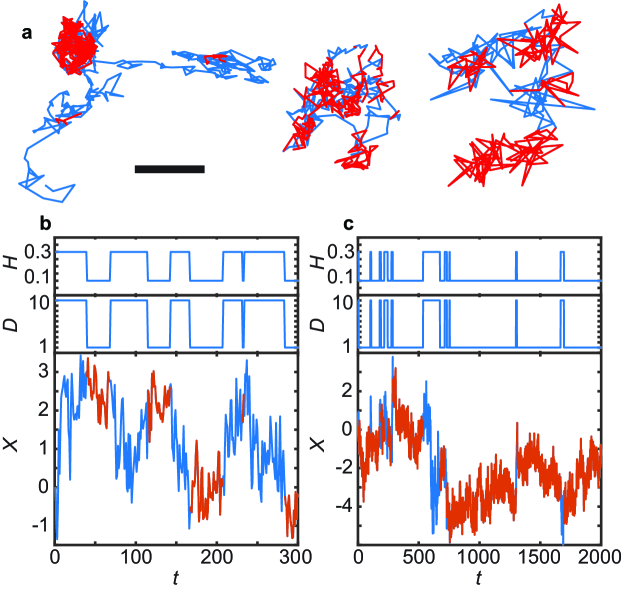
Figure 1: Representative switching FBM trajectories a Experimental trajectories obtained from single-particle tracking of nanocrystals in live HeLa cells. The trajectories exhibit two states, which are identified using the local convex hull, and shown in red and blue sabri2020elucidating . The scale bar is 500 nm. b-c Numerical simulations obtained using Eq. (2). The two states in the trajectories are $D_{1}=1$, $H_{1}=0.1$, and $D_{2}=10$, $H_{2}=0.3$. The upper panels show the Hurst exponent and the diffusivity of the specific trajectories as a function of time. Panel b shows Markovian switching with $\tau=25$, while in panel c one of the states has a power-law waiting time distribution with $\beta=0.7$. The other state has exponentially distributed waiting times with $\tau=15$. The time in panel b is up to 300 in dimensionless units, while that in panel c is up to 2,000, to emphasise the long dwell times in the scale-free system.

A systematic evaluation of the two-state Markovian switching indicates that, in the long time limit, the MSD is simply a weighted average of the MSDs of the two original underlying processes. Given two states $D_{i}$ and $H_{i}$ with mean dwell times $\tau_{i}$, the MSD of the two parent FBM processes are $\langle\overline{\delta_{i}^{2}(\Delta)}\rangle=2D_{i}\Delta^{2H_{i}}$, and the MSD of the switching FBM is

$$\left<\overline{\delta^{2}(\Delta)}\right>=A_{1}\left<\overline{\delta_{1}^{2}(\Delta)}\right>+A_{2}\left<\overline{\delta_{2}^{2}(\Delta)}\right>,$$ (6)

where $A_{i}=\tau_{i}/(\tau_{1}+\tau_{2})$.

Fig. 2 shows the MSD of different simulations built from states with $H=0.1,0.3$ and $D=1,10$. The MSD of the parent FBMs, i.e., without any switching, are shown in Fig. 2a. Next, Fig. 2b shows the MSD when $D$ changes but $H=0.3$ is kept constant and both states have the same mean dwell time $\tau=25$. Interestingly, in this case, the anomalous diffusion exponent is the same as that of the parent FBMs, $\alpha=2H$. Fig. 2c shows a case in which also $H$ changes, while the mean dwell times $\tau_{i}$ are the same in both states. In Fig. 2d, the dwell times are different, with $\tau_{2}=3\tau_{1}$. In all examined cases, the MSD shows excellent agreement with the weighted average as given by Eq. (6).

The PSD of the switching FBM for two states having exponentially distributed dwell times is shown in Fig. 3. Following the same structure as the MSD in Fig. 2, the PSD of the parent FBMs with $H=0.1,0.3$ and $D=1,10$ are shown in Fig. 3a and the PSD of the switching FBM alternating between these states are shown in Figs. 3b-d. These states correspond to subdiffusive FBM. The PSD of FBM with $H>1/2$ depends on the observation time $T$ krapf2019spectral and such cases for which the parent FBMs are superdiffusive will be discussed later. Again, the PSD of the switching process is given by the weighted average

$$\langle S(\omega)\rangle=A_{1}\langle S_{1}(\omega)\rangle+A_{2}\langle S_{2}(\omega)\rangle,$$ (7)

where, once more, $A_{i}=\tau_{i}/(\tau_{1}+\tau_{2})$. The individual PSD of the original subdiffusive FBM is $\langle S(\omega)\rangle\sim 1/\omega^{1+2H}$ and, thus, the switching FBM exhibits a similar spectral dependence,

$$\langle S(\omega)\rangle\sim 1/\omega^{1+\alpha}.$$ (8)

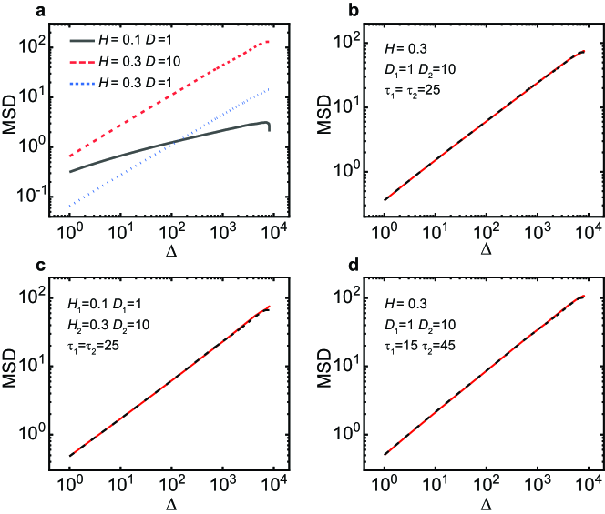
Figure 2: MSD of two-state FBM with Markovian switching exponents. a Standard (single-state) FBM simulated using Eq. (2). b Two-state switching FBM where $D_{1}=1$ and $D_{2}=10$. The Hurst exponent is $H=0.3$ in both states and their mean dwell times are $\tau=25$. The dashed line indicates the average of the two underlying FBM processes. c Two-state switching FBM where the parameters of state 1 are $D_{1}=1$, $H_{1}=0.1$, and the parameters of state 2 are $D_{2}=10$, $H_{2}=0.3$. The mean dwell times are $\tau=25$ for both states. The dashed line indicates the average of the two underlying FBM processes. d Two-state switching FBM with the same parameters as in b, but with mean dwell times 15 and 45 in states 1 and 2, respectively. The dashed line indicates the weighted average of the two underlying FBM processes, i.e., $\langle\overline{\delta^{2}(\Delta)}\rangle=0.25\langle\overline{\delta_{1}^{2}(\Delta)}\rangle+0.75\langle\overline{\delta_{2}^{2}(\Delta)}\rangle$.

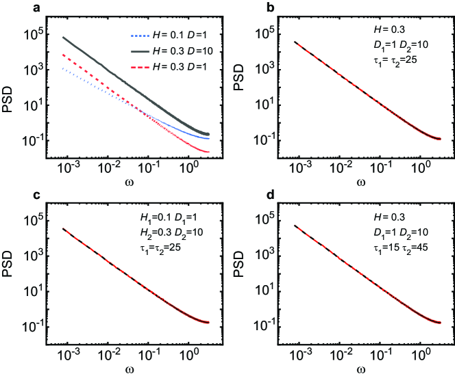
Figure 3: PSD of two-state FBM with Markovian switching exponents. a Standard (single-state) FBM simulated using Eq. (2). b Two-state switching FBM where $D_{1}=1$ and $D_{2}=10$. The Hurst exponent is $H=0.3$ in both states and their mean times are $\tau=25$. The dashed line indicates the average of the two underlying FBM processes. c Two-state switching FBM where the parameters of state 1 are $D_{1}=1$, $H_{1}=0.1$, and the parameters of state 2 are $D_{2}=10$, $H_{2}=0.3$. The mean times are $\tau=25$ for both states. The dashed line indicates the average of the two underlying FBM processes. d Two-state switching FBM with the same parameters as in b, but with time scales 15 and 45 for transitions from states 1 and 2, respectively. The dashed line indicates the weighted average of the two underlying FBM processes, i.e., $\langle S(\omega)\rangle=0.25\langle S_{1}(\omega)\rangle+0.75\langle S_{2}(\omega)\rangle$.

III.2 Processes with scale-free relaxation times

We now turn to study two-state dichotomous processes in which the dwell times in one of the states are random variables with a heavy-tailed distribution, namely, they are distributed according to a Pareto PDF,

$$\psi(t)=\frac{\beta t_{0}^{\beta}}{t^{1+\beta}},\;\;\;t>t_{0},$$ (9)

with scale parameter $t_{0}>0$ and shape parameter $0<\beta<1$. The second state is considered to have exponentially distributed dwell times. Such dichotomous processes, in which one of the states exhibits a dwell time distribution with an exponential tail and the second state has a power-law distribution, have received attention in diverse physical systems sadegh20141 ; sikora2017elucidating ; kurilovich2020complex ; kurilovich2022non . The first 2,000 points of a representative trajectory and its corresponding $H$ and $D$ time series are shown in Fig. 1c.

Because one of the states has a dwell time with infinite mean, the process is expected to exhibit ageing and ergodicity breaking metzler2014anomalous ; weron2017ergodicity ; krapf2019spectral . Fig. 4 shows the MSD and PSD of processes of this type, for which the Hurst exponents of both states are subdiffusive, $H_{i}<1/2$. The dependence on observation time is evident for both the MSD and the PSD. Figs. 4a and c show, respectively, the MSD and PSD of a system in which the Hurst exponent is the same for both states, $H=0.3$, and the generalised diffusion coefficient changes 10-fold. The obtained statistics yield

$$\left<\overline{\delta^{2}(\Delta,T)}\right>\sim(AT^{\beta-1}+2D_{1})\Delta^{2H}$$ (10)

and

$$\langle S(\omega,T)\rangle\sim\frac{CT^{\beta-1}+S_{1}}{\omega^{1+2H}},$$ (11)

where state 1, is the one with power-law sojourn times. The amplitude of the MSD (PSD) of the switching FBM is such that it slowly approaches (in a power-law) to the amplitude of the MSD (PSD) of state 1, see the insets of Figs. 4a and c. To be precise, the MSD converges to $2D_{1}\Delta^{2H}$ and the PSD to $S_{1}/\omega^{1+2H}$, where $S_{1}=2D_{1}\Gamma(2H+1)\sin(\pi H)$ krapf2019spectral . For any experimental time $T$, in the long lag-time limit, the MSD scales as $\Delta^{2H}$ and the PSD scales as $\omega^{-(1+2H)}$.

When the Hurst exponents of the two states are different, the MSD and PSD still converge towards those of the state with power-law sojourn times. However, the results are fairly different in that, now, the MSD dependence on lag time $\Delta$ and the frequency dependence of the PSD have exponents that depend on the experimental time $T$. In this case,

$$\left<\overline{\delta^{2}(\Delta,T)}\right>\sim A(T)\Delta^{\alpha(T)}$$ (12)

and

$$\langle S(\omega,T)\rangle\sim\frac{C(T)}{\omega^{1+\alpha(T)}},$$ (13)

where the amplitudes $A(T)$ and $C(T)$, and the exponents $\alpha(T)$ are given by

$$A(T) =A_{0}T^{\beta-1}+2D_{1},$$

$$C(T) =C_{0}T^{\beta-1}+S_{1},$$ (14)

and

$$\alpha(T)=\alpha_{0}T^{\beta-1}+\alpha_{1},$$ (15)

where $A_{0}$, $C_{0}$, and $\alpha_{0}$ are constants that depend on the occupation fraction in state 1 during the initial time of the process and $\alpha_{1}=2H_{1}$ is the anomalous diffusion exponent of state 1.

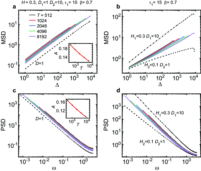
Figure 4: Two-state switching subdiffusive FBM for which one of the states exhibits scale-free dwell times. The MSD and PSD are computed for different observation times $T$. As guides to the eye, the dashed lines show the analysis of ordinary FBM processes. a MSD of two-state switching FBM with the same Hurst exponent $H=0.3$ but different generalised diffusion coefficients, such that $D_{2}=10D_{1}$. The dwell times in the first state are distributed according to a Pareto distribution, such that it is asymptotically a power-law with exponent $\beta=0.7$. The second state has an exponentially distributed dwell time with a mean $\tau=15$. The MSD depends on the observation time. Inset: The amplitude of the MSD decays as a power-law toward the MSD of the state with power-law waiting times, in agreement with Eq. (10). b Two-state FBM for which both the Hurst exponent and the diffusivity change. Namely, $D_{1}=1$, $H_{1}=0.1$, and the parameters of state 2 are $D_{2}=10$, $H_{2}=0.3$. The waiting times in the first state have a heavy-tailed distribution. The second state has exponentially distributed waiting times. c PSD of the simulations in panel a. The inset shows that the amplitude of the PSD decays as a power-law toward the PSD of the state with power-law waiting times, in agreement with Eqs. (12) and (14). d PSD of the simulations in panel b.

III.3 Switching superdiffusive FBM

FBM can be subdiffusive ($H<1/2$) or superdiffusive ($H>1/2$). While the MSD in both cases scales as $\langle\overline{\delta^{2}(\Delta)}\rangle\sim\Delta^{2H}$, the scaling of the PSD differs among the two classes. As discussed above, for subdiffusive FBM, $\langle S(\omega)\rangle\sim 1/\omega^{1+2H}$, but when the FBM is superdiffusive, the frequency scaling of the PSD resembles that of Brownian motion, albeit with a dependence on observation time, $\langle S(\omega,T)\rangle\sim T^{2H-1}/\omega^{2}$ krapf2019spectral . Therefore, the analysis of switching superdiffusive FBM needs separate attention.

Fig. 5 shows the PSD and MSD of switching FBM consisting of two states with the Hurst exponents $H_{1}=0.6$ and $H_{2}=0.8$, and power-law distributed sojourn times in state 2. The outcome involves a dependence on observation time that arises from both the switching mechanism and the FBM itself. Namely, the PSD has a dependence on frequency of the form $1/\omega^{2}$, and a dependence on experimental time with a scaling factor $T^{\alpha(T)-1}$ from the FBM and a scaling factor $(CT^{\beta-1}+S_{1})$ due to the switching between states. In addition, the MSD involves a change in the anomalous diffusion exponent $\alpha$, similar to that in Eq. (15). When the first state is subdiffusive ($H_{1}<0.5$, data not shown) the obtained results do not exhibit any difference from those when both processes are superdiffusive. Namely for the mixed sub- and superdiffusive case, the PSD and MSD asymptotically converge to those of the state with power-law dwell times.

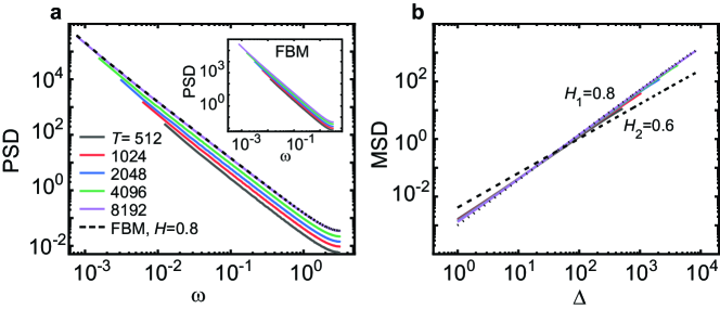
Figure 5: Two-state superdiffusive FBM for which one of the states exhibits scale-free dwell times. The PSD (panel a) and MSD (panel b) are computed for different realisation times. The process consists of two states with $H_{1}=0.6$ and $H_{2}=0.8$. The sojourn times in state 1 are exponentially distributed and those of state 2 have a heavy-tailed distribution with $\beta=0.7$. The inset in panel a shows the ageing in the traditional FBM for $H=0.8$ in dependence of the observation time $T$.

III.4 Analysis of experimental data: quantum dots in the cytoplasm of live cells

In order to highlight the use of the switching FBM process in the analysis of real world data, we analyse the PSD of quantum dot trajectories in the cytoplasm of living HeLa cells. These data have been thoroughly analysed in terms of their MSD, velocity autocorrelation function, and distribution of displacements sabri2020elucidating , as well as via the use of a hidden Markov model approach janczura2021identifying , the intermediate scattering function dieball2022scattering and the decomposition of the Hurst exponent into components involving non-stationarity, heavy-tailed distributions, and long-range correlations vilk2022unravelling . These extensive analyses show that the diffusive motion of quantum dots stochastically alternates between two states, with both states having correlations of the type of subdiffusive FBM. Thus, quantum dot dynamics in the cytoplasm presents an excellent system to test some of the predictions of the switching FBM model. The switching between the two states in this experimental system obeys a Markov process and the MSD is subdiffusive with a mean anomalous diffusion exponent $\alpha=0.59$ sabri2020elucidating ; janczura2021identifying . Our predictions indicate that the PSD should not exhibit ageing effects and its spectral dependence, according to Eq. (8), is expected to be $\langle S(\omega)\rangle\sim 1/\omega^{1+\alpha}$.

The difficulty in the analysis of experimental data lies in the fact that long trajectories are not available because eventually particles leave the field of view, or they become dark (due to long blinking in the case of quantum dots or photobleaching in the case of organic fluorophores). The analysed quantum dot data consist of 3,834 trajectories of only 100 time points each. Such short trajectories present unique problems in the statistical analysis. Further, experimental data is unavoidably corrupted by experimental noise, such as static and dynamic localisation errors inherent to single-particle tracking savin2005static .

The MSD and PSD analysis of quantum dot trajectories along the projections on one axis is presented in Fig. 6. The MSD at short times is seen to scale as $\langle\overline{\delta^{2}(\Delta)}\rangle\sim\Delta^{\alpha}$ with $\alpha=0.59$. Despite the short length of the trajectories and the presence of localisation errors, the agreement with the predicted PSD is remarkable. The analysis is performed for three observation times ($T=1.6$ s, $3.2$ s, and $6.4$ s) consisting of 16, 32, and 64 time points. The three PSDs are observed to fall on the same line, i.e., there is no evident ageing, and the slope of the PSD agrees with the prediction $1/\omega^{1.59}$.

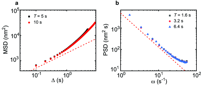
Figure 6: Analysis of experimental trajectories of quantum dots in the cytoplasm of live mammalian cells. The projection of quantum dot trajectories along the $x$ axis is analysed, for different measurement times $T$, in terms of a the MSD and b the PSD. For different measurement times, the MSDs overlap (no ageing) and exhibits a behaviour $\langle\overline{\delta^{2}(\Delta)}\rangle\sim\Delta^{0.59}$ at short lag-times, indicating an apparent anomalous diffusion exponent $\alpha=0.59$, as obtained previously by averaging the anomalous diffusion exponents of individual trajectories sabri2020elucidating . In agreement with the predictions for Markov switching, the PSDs overlap for the three measurement times and show a scaling $\langle S(\omega,T)\rangle\sim 1/\omega^{1.59}$. The dashed red lines are guides to the eye indicating a scaling $\Delta^{0.59}$ in panel a and $\omega^{1.59}$ in panel b.

III.5 Distribution of displacements

Both the MSD and PSD of switching FBM with exponentially-distributed dwell times resemble those of classical FBM, making it impossible to rely solely on these statistics to identify the model. The problem is less severe when the distribution of dwell times have heavy tails because in these cases, the MSD and PSD exhibit ageing in stark contrast to ordinary FBM processes. One clear signature of heterogeneous or intermittent processes lies in the distribution of displacements which is typically non-Gaussian. Fig. 7 shows the distribution of displacements for switching FBM realisations with exponential dwell time distribution. Here we present a process with characteristic dwell times $\tau=25$ and displacements over times that span a scale from much shorter to much longer times than this characteristic time. Namely, displacements were computed at four different times, $\Delta t=1$, $5$, $50$, and $250$.

For times much shorter than the characteristic time (Figs. 7a and b, $\Delta t\ll\tau$), the distribution of displacements is very close to the sum of two Gaussian functions. Specifically, the two parent FBM have a normal distribution of displacements with standard deviations $\sigma_{1}$ and $\sigma_{2}$. Then, the switching FBM process has a distribution that is a sum of two Gaussians with the same standard deviations, namely $P_{\Delta t}(\Delta x)=\sum_{i}A_{i}\exp(\Delta x^{2}/2\sigma_{i}^{2})$, where $\sigma_{i}^{2}\propto\Delta t^{2H_{i}}$.

For times longer than the characteristic dwell time ($\Delta t>\tau$), the situation is rather different. In fact, as the times over which the displacements are computed become much longer than the characteristic time ($\Delta t\gg\tau$), the distribution of displacements approaches a normal distribution. Fig. 7d shows the behaviour at time $\Delta t=250$, i.e., $\Delta t=10\tau$, and here the deviations from Gaussianity are very small.

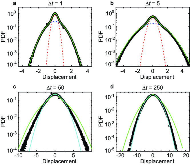
Figure 7: Distributions of displacements for switching FBM process are not Gaussian. The PDF of the displacements is estimated for a process with Markov switching, whose mean dwell time in each state is $\tau=25$, the Hurst exponent of both states is $H=0.3$ and the diffusivities are $D_{1}=1$ and $D_{2}=10$. The times over which the displacements are computed are (a) $\Delta t=1$, (b) $\Delta t=5$, (c) $\Delta t=50$, and (d) $\Delta t=250$. In panels (a) and (b) (shoter times), the two coloured dashed lines show a decomposition into two Gaussian functions with the standard deviations of the distributions of the two parent FBM. The green solid line indicates the superposition of the two Gaussian functions. In panels (c) and (d) (longer times), the solid green line shows a superposition of two Gaussian functions and the thick cyan line shows a fit to a single Gaussian peak.

IV Discussion and Conclusions

We studied FBM, a stochastic process driven by long-ranged correlated Gaussian noise, in which both diffusion coefficient and Hurst exponent are stochastic processes themselves. We modelled these for cases with exponential and scale-free dwell time distributions. This model belongs to the class of doubly-stochastic processes (both the driving noise but also the model parameters are stochastic) that currently receive increased attention. In particular, we analysed the time-averaged MSD and the PSD of the emerging dynamics.

Markovian switching resembles ordinary FBM both in terms of the PSD and the MSD. Thus, these metrics are not sufficient to dissect the process and recognise that it is not driven by a single FBM. In other words, the switching dynamic does not have any clear fingerprint in the MSD or the PSD. An additional statistic that provides information on the switching can be obtained from the distribution of displacements, which in this case is non-Gaussian (Fig. 7). Such distributions have also been observed experimentally, e.g., in quantum dot trajectories in the cytoplasm for which the non-Gaussian nature of the displacement hints at a more complex process than FBM. However, as the displacements are computed over increasingly longer times in the switching FBM model, deviations from Gaussianity subside. Such effects are also observed for experimental data, where, as time increases, the distribution of displacements approaches a Gaussian distribution sabri2020elucidating . Thus, in order to identify a Markov switching process, it is necessary to obtain measurements with a temporal resolution better than the characteristic dwell times. If this type of data is available, the two states can be identified using a change point detection tool lanoiselee2017unraveling ; sikora2017elucidating ; wagner2017classification .

Going beyond Markov switching, scale-free processes, in which at least one of the states has a heavy-tailed distribution of dwell times are inherently non-ergodic and have non-stationary increments. The quintessential process of this type is the continuous time random walk metzler2014anomalous . When one of the states has a heavy-tailed distribution of dwell times, both the MSD and the PSD depend explicitly on time.

An interesting case is that of superdiffusive FBM, based on persistent active stochastic dynamics, such as intracellular motion driven by molecular motors in living cells reverey2015superdiffusion or animal motion vilk2022unravelling ; vilk2022ergodicity . This should not be taken to indicate that active motion will always lead to superdiffusion; as soon as there exists a finite persistence time, the motion will be Brownian at times longer than this time scale romanczuk2012active ; lemaitre2023non . Moreover, transient superdiffusion may arise in passive systems, such as bulk-mediated diffusion campagnola2015superdiffusive . Superdiffusive FBM has a PSD that depends on experimental time $T$ krapf2019spectral and, thus, also the Markovian switching for which at least one of the states is superdiffusive exhibits a PSD that depends on realisation time. However, the PSD is still found as a weighted average of the parent (time-dependent) PSDs.

A simple visual inspection allows one to determine whether the two states in the switching FBM have the same Hurst exponent $H$. In the case that $H$ does not change, the anomalous diffusion exponent as determined by the PSD and the MSD does not depend on the experimental time $T$. In such cases, the MSD (and PSD) exhibit the same slope when visualised in a log-log plot for different realisation times (Fig. 4a). The MSD (PSD) converges to the MSD (PSD) of the FBM with power-law waiting times. However, the convergence has a power-law character. When $H$ changes, the MSD (PSD) still converges to the state with heavy-tailed waiting times but in this case each experimental time exhibits a different exponent. We foresee that switching FBM with different Hurst exponents can have multiple direct applications in cell biology, such as the heterogeneous dynamics of intracellular endosomes fedotov .

To simplify the analyses, we restricted our work in switching FBM to two states. However, there is no actual limit to the number of states that can be included. In particular, a multi-state Markov process can include a full transition matrix between the different states. This work opens the way to modelling heterogeneous anomalous dynamics, where the underlying heterogeneity leads to dynamic transitions. Moreover, the results obtained allow for future theoretical investigations of correlated random walks in complex systems where regime changes dominate the transport.

References

Appendix A. Extended numerical methods

Here, we describe the simulation procedure of the switching FBM.

IV.1 General case.

We first consider the general case since Eq. (2), which defines switching FBM, is a special case of the integral representation of the process

$$X(t)=\int_{-\infty}^{\infty}f_{t}(s)\mathrm{d}B(s).$$ (16)

To simulate the process $X(t)$, we need to numerically approximate the integral (16). Usually, this is done in two steps: first, truncating the limits of integration (this step depends on the form of $f_{t}$), and, second, approximating the truncated integral by a Riemann sum.

First step. For $M_{1},M_{2}\in\mathbb{R}$ we have

$$\int_{-\infty}^{\infty}f_{t}(s)\mathrm{d}B(s)\approx\int_{M_{1}}^{M_{2}}f_{t}(s)\mathrm{d}B(s).$$ (17)

In general, it is advised to choose reasonably large values $M_{1}$ and $M_{2}$. In practice, the truncation parameters may also depend on $t$.
Second step. We divide the interval $[M_{1},M_{2}]$ into $I$ equal parts of length $\lambda=\frac{M_{2}-M_{1}}{I}$, and consider points $s_{i}=M_{1}+i\lambda$ for $i=0,1,\ldots,I$. Then

$$\int_{M_{1}}^{M_{2}}f_{t}(s)\mathrm{d}B(s)=\sum_{i=0}^{I-1}\int_{s_{i}}^{s_{i+1}}f_{t}(s)\mathrm{d}B(s).$$ (18)

Now, we assume that each subinterval $\left[s_{i},s_{i+1}\right)$ is small ($I$ is large) and we apply a Riemann (or Euler) type of approximation, i.e., we calculate the function $f_{t}(s)$ at $s_{i}$ for $i=0,1,\ldots,$ $I-1$ and obtain

$$X(t)\approx\sum_{i=0}^{I-1}\int_{s_{i}}^{s_{i+1}}f_{t}(s_{i})\mathrm{d}B(s)=\sum_{i=0}^{I-1}f_{t}(s_{i})\left[B(s_{i+1})-B(s_{i})\right]=\sum_{i=0}^{I-1}f_{t}(s_{i})\xi_{i},$$ (19)

where $\xi_{i}$ are i.i.d. random variables with $N(0,\lambda)$ distribution.

Finally, we note that to simulate a trajectory of the process $X(t)$ at various time points $t_{1},t_{2},\ldots,t_{n}$, we rely on one sequence of $\xi_{i}$’ s (a single trajectory of the process $B(s)$ for all possible values of $s$).

IV.2 Switching FBM.

In this particular case, to generate a single trajectory of switching FBM we first need to generate trajectories of the processes $D(s)$ and $H(s)$. We do this by generating waiting times from the selected distribution. Then, having a single trajectory of both $D$ and $H$ we use the approximation given in Eq. (19) with

$$f_{t}(s)=\sqrt{2D(s)H(s)}(t-s)^{H(s)-\frac{1}{2}}\mathbf{1}_{\left[0,t\right)}(s),\;t\in[0,T].$$

The points $s_{0},s_{1},\ldots,s_{I}$ are chosen so that $s_{0}=M_{1}=0$ and $s_{I}=M_{2}=T$. In all simulations performed, the length of the trajectories $n=2^{13}$, $t_{i}=i\Delta_{t},i=0,1,\ldots,n$, $\Delta_{t}=\frac{T}{n}$ and $I=50n$. Thus, to calculate a next time step $X(t_{j})$ we use an additional 50 new steps $s_{i}$, e.g., to calculate $X(t_{1})$ we use $f_{t_{1}}(s)$ in points $s_{0},s_{1},\ldots,s_{49}$, to calculate $X(t_{2})$ we use $f_{t_{2}}(s)$ in points $s_{0},s_{1},\ldots,s_{49},s_{50},\ldots,s_{99}$, and so on.

References

- (1) Levi V and Gratton E 2007 Cell Biochemistry and Biophysics 48 1–15
- (2) Manzo C and Garcia-Parajo M F 2015 Reports on Progress in Physics 78 124601
- (3) Barkai E, Garini Y and Metzler R 2012 Physics Today 65(8) 29
- (4) Höfling F and Franosch T 2013 Reports on Progress in Physics 76 046602
- (5) Krapf D and Metzler R 2019 Physics Today 72(9) 48–54
- (6) Dietrich C, Yang B, Fujiwara T, Kusumi A and Jacobson K 2002 Biophysical Journal 82 274–284
- (7) Knight J D and Falke J J 2009 Biophysical Journal 96 566–582
- (8) Campagnola G, Nepal K, Schroder B W, Peersen O B and Krapf D 2015 Scientific Reports 5 17721
- (9) Manzo C, Torreno-Pina J A, Massignan P, Lapeyre Jr G J, Lewenstein M and Garcia Parajo M F 2015 Physical Review X 5 011021
- (10) Metz M J, Pennock R L, Krapf D and Hentges S T 2019 Scientific Reports 9 7297
- (11) Mosqueira A, Camino P A and Barrantes F J 2020 Journal of Neurochemistry 152 663–674
- (12) Weigel A V, Simon B, Tamkun M M and Krapf D 2011 Proceedings of the National Academy of Sciences 108 6438–6443
- (13) Akin E J, Solé L, Johnson B, El Beheiry M, Masson J B, Krapf D and Tamkun M M 2016 Biophysical Journal 111 1235–1247
- (14) He W, Song H, Su Y, Geng L, Ackerson B J, Peng H and Tong P 2016 Nature Communications 7 11701
- (15) Bronstein I, Israel Y, Kepten E, Mai S, Shav-Tal Y, Barkai E and Garini Y 2009 Physical Review Letters 103 018102
- (16) Moon S L, Morisaki T, Khong A, Lyon K, Parker R and Stasevich T J 2019 Nature Cell Biology 21 162–168
- (17) Ruhnow F, Zwicker D and Diez S 2011 Biophysical Journal 100 2820–2828
- (18) Nixon-Abell J, Obara C J, Weigel A V, Li D, Legant W R, Xu C S, Pasolli H A, Harvey K, Hess H F, Betzig E et al. 2016 Science 354 aaf3928
- (19) Speckner K, Stadler L and Weiss M 2018 Physical Review E 98 012406
- (20) Korabel N, Han D, Taloni A, Pagnini G, Fedotov S, Allan V and Waigh T A 2021 Entropy 23 958
- (21) Weihs D, Mason T G and Teitell M A 2006 Biophysical Journal 91 4296–4305
- (22) Etoc F, Balloul E, Vicario C, Normanno D, Liße D, Sittner A, Piehler J, Dahan M and Coppey M 2018 Nature Materials 17 740–746
- (23) Sabri A, Xu X, Krapf D and Weiss M 2020 Physical Review Letters 125 058101
- (24) Berg H C 2000 Physics Today 53 24–29
- (25) Sims D W, Humphries N E, Hu N, Medan V and Berni J 2019 Elife 8 e50316
- (26) Hays G C, Bastian T, Doyle T K, Fossette S, Gleiss A C, Gravenor M B, Hobson V J, Humphries N E, Lilley M K, Pade N G et al. 2012 Proceedings of the Royal Society B: Biological Sciences 279 465–473
- (27) Vilk O, Aghion E, Avgar T, Beta C, Nagel O, Sabri A, Sarfati R, Schwartz D K, Weiss M, Krapf D et al. 2022 Physical Review Research 4 033055
- (28) Vilk O, Orchan Y, Charter M, Ganot N, Toledo S, Nathan R and Assaf M 2022 Physical Review X 12 031005
- (29) Bouchaud J P 2005 Chaos: An Interdisciplinary Journal of Nonlinear Science 15 026104
- (30) Scalas E 2006 Physica A: Statistical Mechanics and its Applications 362 225–239
- (31) Edery Y, Scher H and Berkowitz B 2010 Water Resources Research 46 W07524
- (32) Weigel A V, Ragi S, Reid M L, Chong E K, Tamkun M M and Krapf D 2012 Physical Review E 85 041924
- (33) Wu H and Schwartz D K 2020 Accounts of Chemical Research 53 2130–2139
- (34) Metzler R, Jeon J H, Cherstvy A G and Barkai E 2014 Physical Chemistry Chemical Physics 16 24128–24164
- (35) Krapf D 2015 Current Topics in Membranes 75 167–207
- (36) Krapf D, Marinari E, Metzler R, Oshanin G, Xu X and Squarcini A 2018 New Journal of Physics 20 023029
- (37) Meroz Y and Sokolov I M 2015 Physics Reports 573 1–29
- (38) Robson A, Burrage K and Leake M C 2013 Philosophical Transactions of the Royal Society B: Biological Sciences 368 20120029
- (39) Thapa S, Lomholt M A, Krog J, Cherstvy A G and Metzler R 2018 Physical Chemistry Chemical Physics 20 29018–29037
- (40) Muñoz-Gil G, Volpe G, Garcia-March M A, Aghion E, Argun A, Hong C B, Bland T, Bo S, Conejero J A, Firbas N et al. 2021 Nature Communications 12 6253
- (41) Seckler H and Metzler R 2022 Nature Communications 13 6717
- (42) Seckler H, Szwabiński J and Metzler R 2023 Journal of Physical Chemistry Letters 14 7910
- (43) Gajowczyk M and Szwabiński J 2021 Entropy 23 649
- (44) Muñoz-Gil G, Garcia-March M A, Manzo C, Martín-Guerrero J D and Lewenstein M 2020 New Journal of Physics 22 013010
- (45) Montroll E W and Weiss G H 1965 Journal of Mathematical Physics 6 167–181
- (46) Scher H and Lax M 1973 Physical Review B 7 4491
- (47) Scher H, Shlesinger M F and Bendler J T 1991 Physics Today 44 26–34
- (48) Kolmogorov A N 1940 Acad. Sci. URSS (NS) 26 115–118
- (49) Mandelbrot B B and Van Ness J W 1968 SIAM Review 10 422–437
- (50) Szymanski J and Weiss M 2009 Physical Review Letters 103 038102
- (51) Magdziarz M, Weron A, Burnecki K and Klafter J 2009 Physical Review Letters 103 180602
- (52) Sadegh S, Higgins J L, Mannion P C, Tamkun M M and Krapf D 2017 Physical Review X 7 011031
- (53) Lampo T J, Stylianidou S, Backlund M P, Wiggins P A and Spakowitz A J 2017 Biophysical Journal 112 532–542
- (54) Jeon J H, Javanainen M, Martinez-Seara H, Metzler R and Vattulainen I 2016 Physical Review X 6 021006
- (55) Balcerek M, Burnecki K, Thapa S, Wyłomańska A and Chechkin A 2022 Chaos: An Interdisciplinary Journal of Nonlinear Science 32 093114
- (56) Jeon J H, Tejedor V, Burov S, Barkai E, Selhuber-Unkel C, Berg-Sørensen K, Oddershede L and Metzler R 2011 Physical review letters 106 048103
- (57) Tabei S A, Burov S, Kim H Y, Kuznetsov A, Huynh T, Jureller J, Philipson L H, Dinner A R and Scherer N F 2013 Proceedings of the National Academy of Sciences 110 4911–4916
- (58) Deng W and Barkai E 2009 Physical Review E 79 011112
- (59) Choquet D and Triller A 2013 Neuron 80 691–703
- (60) Weigel A V, Tamkun M M and Krapf D 2013 Proceedings of the National Academy of Sciences 110 E4591–E4600
- (61) Sikora G, Wyłomańska A, Gajda J, Solé L, Akin E J, Tamkun M M and Krapf D 2017 Physical Review E 96 062404
- (62) Weron A, Burnecki K, Akin E J, Solé L, Balcerek M, Tamkun M M and Krapf D 2017 Scientific Reports 7 5404
- (63) Arcizet D, Meier B, Sackmann E, Rädler J O and Heinrich D 2008 Physical Review Letters 101 248103
- (64) Han D, Korabel N, Chen R, Johnston M, Gavrilova A, Allan V J, Fedotov S and Waigh T A 2020 Elife 9 e52224
- (65) Loverdo C, Benichou O, Voituriez R, Biebricher A, Bonnet I and Desbiolles P 2009 Physical Review Letters 102 188101
- (66) Andreao R V, Dorizzi B and Boudy J 2006 IEEE Transactions on Biomedical Engineering 53 1541–1549
- (67) Khanagha V, Daoudi K, Pont O and Yahia H 2014 Digital Signal Processing 35 86–94
- (68) Cetin M and Comert G 2006 Transportation Research Record 1965 23–31
- (69) Janczura J and Weron R 2013 AStA Advances in Statistical Analysis 97 239–270
- (70) Lux T and Morales-Arias L 2010 Computational Statistics & Data Analysis 54 2676–2692
- (71) Edelhoff H, Signer J and Balkenhol N 2016 Movement Ecology 4 1–21
- (72) Stanislavsky A, Burnecki K, Magdziarz M, Weron A and Weron K 2009 The Astrophysical Journal 693 1877
- (73) Vasas K, Elek P and Márkus L 2007 Journal of Statistical Planning and Inference 137 3113–3126
- (74) Lévy P 1953 Random functions: general theory with special reference to Laplacian random functions 12 (University of California Press)
- (75) Wang W, Balcerek M, Burnecki K, Chechkin A V, Janušonis S, Ślęzak J, Vojta T, Wyłomańska A and Metzler R 2023 Phys. Rev. Res. 5 L032025
- (76) Krapf D, Lukat N, Marinari E, Metzler R, Oshanin G, Selhuber-Unkel C, Squarcini A, Stadler L, Weiss M and Xu X 2019 Physical Review X 9 011019
- (77) Sadegh S, Barkai E and Krapf D 2014 New Journal of Physics 16 113054
- (78) Kurilovich A A, Mantsevich V N, Stevenson K J, Chechkin A V and Palyulin V V 2020 Physical Chemistry Chemical Physics 22 24686–24696
- (79) Kurilovich A A, Mantsevich V N, Mardoukhi Y, Stevenson K J, Chechkin A V and Palyulin V V 2022 Physical Chemistry Chemical Physics 24 13941–13950
- (80) Janczura J, Balcerek M, Burnecki K, Sabri A, Weiss M and Krapf D 2021 New Journal of Physics 23 053018
- (81) Dieball C, Krapf D, Weiss M and Godec A 2022 New Journal of Physics 24 023004
- (82) Savin T and Doyle P S 2005 Biophysical Journal 88 623–638
- (83) Lanoiselée Y and Grebenkov D S 2017 Physical Review E 96 022144
- (84) Wagner T, Kroll A, Haramagatti C R, Lipinski H G and Wiemann M 2017 PLoS ONE 12 e0170165
- (85) Reverey J F, Jeon J H, Bao H, Leippe M, Metzler R and Selhuber-Unkel C 2015 Scientific Reports 5 1–14
- (86) Romanczuk P, Bär M, Ebeling W, Lindner B and Schimansky-Geier L 2012 The European Physical Journal Special Topics 202 1–162
- (87) Lemaitre E, Sokolov I M, Metzler R and Chechkin A V 2023 New Journal of Physics 25 013010