Dimensionless Numbers Reveal Distinct Regimes in the Structure and Dynamics of Pedestrian Crowds

Abstract

In fluid mechanics, dimensionless numbers like the Reynolds number help classify flows. We argue that such a classification is also relevant for crowd flows by putting forward the dimensionless Intrusion and Avoidance numbers. Using an extensive dataset, we show that these delineate regimes that are characterized by distinct structural signatures, best probed in terms of distances at low Avoidance number and times-to-collision at low Intrusion number. These findings prompt a perturbative expansion of the agent-based dynamics; the generic models thus obtained perform well in (and only in) the regime in which they were derived.

Crowds often look like an ocean made of hundreds or thousands of heads, ruffled by ripples and waves [1], moving in synchrony or not; this impression struck poets [2] long before it inspired scientists [3, 4]. Yet, even as of now, pedestrian dynamics as a discipline does not stand on the same footing as fluid mechanics. In the latter field, the classical motion of particles at the microscale is governed by an exact equation, Newton’s law, whose homogenization yields the universal Navier-Stokes equation. In practice, modelers resort to a plethora of approximate schemes (e.g., Stokesian dynamics, lattice Boltzmann methods, Euler equations for inviscid flows) but the choice among these is guided, and theoretically bolstered, by the calculation of dimensionless numbers, such as the Reynolds number and the Mach number.

On the other hand, a zoo of models for pedestrian dynamics co-exist (see e.g. [5, 6, 7, 8]) and the realm of applicability of each is ill-defined. The crowd’s density is generally used to delineate different regimes, for instance the levels of service defined by Fruin for crowds [9, 10] Each level is marked by a dominant behavior: (un)avoidable contact, necessity to change gait, possibility to turn around, etc. and it has been argued that as the density changes crowd dynamics should be controlled by distinct laws [11]. However, the watershed between the regimes are arbitrary. Even from a practical standpoint, for safety assessments, crowds at similar densities may present contrasted characters and risk profiles. Consider the difference between a densely packed, but static audience in a concert hall and people vying for escape in an emergency evacuation [12]. Recently, yearning for a better classification of these scenarios, it was proposed to gauge congestion on the basis of a dimensionless number related to the vorticity of the velocity field, instead of the density [13]. This quantity is practically relevant, notably for safety issues, but gives no insight into the determinants of pedestrian dynamics at the microscale.

In this Letter, we argue that in common scenarios pedestrian dynamics are dominated by two variables, rendering the ideas of preservation of personal space (proxemics) and anticipation of collisions. Their averages over the crowd define dimensionless parameters that delineate distinct regimes of crowd flow. The nature of the structural arrangement of the crowd is found to differ markedly between these regimes and their dynamics can be asymptotically approached by a perturbative analysis around the non-interacting situation. Like the Reynolds number in fluid mechanics, these dimensionless numbers help gauge the range of validity of pedestrian models.

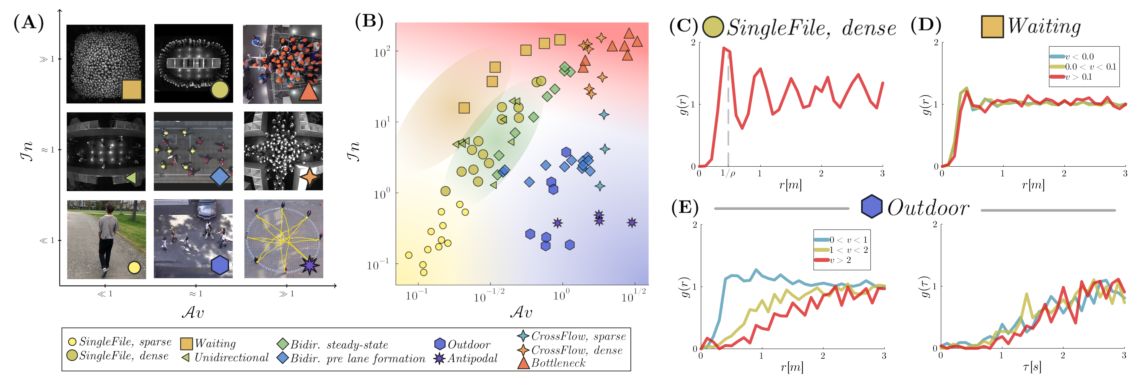
Figure 1: Delineation of crowd flow regimes with the dimensionless numbers $\mathcal{I}n$ and $\mathcal{A}v$. (A) Sketch of the expected diagram, illustrated with snapshots from the collated datasets (described in Appendix A). (B) Empirical diagram obtained from various pedestrian datasets. Each datapoint corresponds to one experimental run or observational sequence. The experimental data from SingleFile and CrossFlow were split into a sparse and a dense dataset. Coloured gradients are visual guides, to indicate different regimes. (C) pdf for one run of the SingleFile, dense dataset. (D) pdf for the Waiting dataset and (E) for the Outdoor dataset. The curves are binned according to the rate of approach $v=-dr/dt$ (given in $m/s$). As for (D) the pdf is well parameterised by $r$ and poorly by $\tau$ (see Fig. $3$ in Appendix C) and in (E) vice versa.

Psychological studies on proxemics indicate that people pay attention to their personal space, defined as "the area individuals maintain around themselves into which others cannot intrude without arousing discomfort" [14], more than to global density [15]. To avoid possible ambiguities in the definition of a local density and underscore the transition from no-contact dynamics to contacts and pushes, we introduce the following intrusion variable based on the center-to-center distance $r_{ij}$,

$$\mathcal{I}n_{i}=\sum_{j\in\mathcal{N}_{i}}\underset{\mathcal{I}n_{ij}}{\underbrace{\left(\frac{r_{\text{soc}}-\ell_{\text{min}}}{r_{ij}-\ell_{\text{min}}}\right)^{2}}},$$ (1)

which represents the sum of areal encroachments of other agents $j$ on $i$’s personal space. $\mathcal{I}n_{i}$ vanishes for isolated pedestrians and diverges at physical contact. For simplicity, we overlook anisotropic effects and assume uniform circular shapes for the pedestrian bodies and personal spaces, of diameter $\ell_{\text{min}}=0.2\,\mathrm{m}$ and radius $r_{\text{soc}}=0.8$ $m$, respectively. The sum runs over the set $\mathcal{N}_{i}$ of all close neighbors $j$ of $i$, here defined by $r_{ij}\leqslant 3\,r_{\text{soc}}$. That the intrusions of diverse neighbors should be added up makes sense for physical contacts (superposition of mechanical forces), but also for proxemic behavior [16, 17].

While this variable gives a sense of the level of crowding, it neither provides a full reflection of psychological experience (feeling of congestion) in the midst of the crowd [18, 13], nor fully controls the agent’s dynamics: when two people $i$ and $j$ run towards each other, they will not behave as though they were isolated, even though they may still be separated by several meters, hence, $\mathcal{I}n_{ij}\to 0$. This anticipatory behaviour is well captured by an anticipated time-to-collision (TTC) $\tau_{ij}$, defined as the delay until the first collision if both $i$ and $j$ keep their current velocities ($\tau_{ij}=\infty$ if no collision is expected). Humans are indeed capable of identifying the most imminent collision between multiple objects and estimating TTCs [19], notably via purely optical quantities, namely, the optical angle divided by its derivative [20]. Experiments showed that humans use the TTC to decide ‘when’ to avoid an approaching pedestrian [21]. Accordingly, we quantify the risk of an imminent collision through an avoidance variable

$$\mathcal{A}v_{i}=\sum_{j\in\mathcal{N}_{i}^{\prime}}\underset{\mathcal{A}v_{ij}}{\underbrace{\frac{\tau_{0}}{\tau_{ij}}}},$$ (2)

where $\tau_{0}=3\,\mathrm{s}$ denotes the timescale above which collisions are hardly dreaded. Here, in contrast with Eq. 1, the set of neighbors $\mathcal{N}_{i}^{\prime}$ is restricted to the agent with the shortest $\tau_{ij}$, i.e., the most imminent risk. Indeed, for collision avoidance, it has been ascertained that participants immersed in a virtual crowd tend to fixate a particular agent with a high risk of collision just before performing an avoidance maneuver around this person [22].

With these two variables in hand, one can hope for a finer delineation of pedestrian streams than with the traditional density-based levels of service. To this end, the foregoing agent-centred variables are averaged over the $N(t)$ agents observed in the crowd at time $t$, and then over time. This average defines the dimensionless Avoidance number $\mathcal{A}v$ and Intrusion number $\mathcal{I}n$. As $\mathcal{A}v$ should quantify the urgency of expected collisions we only consider data points with a finite TTC in the average. Especially in the sparse datasets, this allows to focus on the parts where interactions occur. Figure 1A illustrates the regimes of crowd flow that one would intuitively expect to find in a diagram parametrized by $\mathcal{A}v$ and $\mathcal{I}n$, using exemplary cases. The bottom left corner, $\mathcal{I}n,\mathcal{A}v\ll 1$, corresponds to very sparse crowds with hardly any interactions. As one moves up the $\mathcal{I}n-$axis, the setting gets more crowded, and pedestrians are eager to maintain a certain social distance with respect to others, as in a unidirectional flow. When $\mathcal{I}n\gg 1$, personal space can no longer be preserved and physical contact may eventually be unavoidable, as in a tightly packed static crowd (Waiting scenario). A very different way to depart from the non-interacting case is to consider people walking or running towards each other. This is well approximated by the beginning of an Antipodal experiment, in which participants initially positioned all along the circumference of a circle (with $\mathcal{I}n\ll 1$) are asked to reach the antipodal position. This induces conflicting moves, with risks of collision in the centre of the circle, hence $\mathcal{A}v\gg 1$. Finally, competitive evacuations though a bottleneck exemplify the regime of large $\mathcal{I}n$ and $\mathcal{A}v$, which features contacts, pushes, as well as conflicting moves.

These are of course idealized expectations. To test them, we have collated an extensive dataset of pedestrian trajectories, including controlled experiments (single-file motion [23], bottleneck flows [24], corridor flows [25, 26, 27], antipodal scenarios [28]) and empirical observations in outdoor settings [29, 30]; further details about these scenarios and the way we have smoothed out head sways from the trajectories can be found in Appendix A. For each scenario and each realization, we have computed $\mathcal{A}v(t)$ and $\mathcal{I}n(t)$ every $0.5\,$s, and averaged over the whole quasi-stationary state (unless otherwise stated).

Figure 1B shows that the idealized diagram worked out intuitively (Fig. 1A) is largely corroborated by the empirical datasets. Indeed, single files of amply spaced pedestrians are found in the bottom left corner, at small $\mathcal{I}n$ and $\mathcal{A}v$, whereas the top of the diagram, at large $\mathcal{I}n$, is occupied by situations in which physical contacts are almost inevitable. More interestingly, unidirectional flows and cross-flows may have similar $\mathcal{I}n$ numbers, but they are distinguished by $\mathcal{A}v$, which takes larger values for cross-flows, prone to more conflicts. In the same vein, antipodal maneuvers have intrusion numbers comparable to those of some typical outdoor scenarios, but larger avoidance numbers. Note that the $\mathcal{I}n$ and $\mathcal{A}v$ axes have been plotted orthogonally, whereas skewed axes should in principle be used if the variables exhibit some correlations; this does not alter the topology of the diagram, however. Nor do variations of the (somewhat arbitrary) precise definitions of $\mathcal{I}n$ and $\mathcal{A}v$, see Appendix B.

In practice, the visual delineation of regimes on the diagram of Fig. 1B appears sensible. But its physical relevance will only transpire if the delineated regimes exhibit constitutive differences. Remarkably, we find a major difference in the arrangement of the crowd, not in terms of static symmetry of the structure (which distinguishes, say, a liquid from a crystal), but in the nature of this self-organized ‘structure’, i.e., more pragmatically, in the variables that characterize it. Drawing inspiration from condensed matter physics and following [31], we use as structural probe the pair-distribution function (pdf) $g(x)=P(x)/P_{\text{NI}}(x)$ between pedestrians, which quantifies the probability that two interacting pedestrians are found a given distance $x$ apart, renormalized by the probability $P_{\text{NI}}$ of measuring this distance for pedestrians that do not interact. This probability can be approximated by randomizing the time or space information (cf. Appendix C).

Starting from the origin ($\mathcal{I}n,\mathcal{A}v=0$) and moving up along the $\mathcal{I}n$-axis while keeping $\mathcal{A}v\ll 1$, the crowd gets structured in real space, as evidenced by its radial pdf $g(r)$, where $r$ is the Euclidean spacing between people. This is conspicuous for one-dimensional configurations; indeed, the pdf of dense single files (Fig. 1C) develops a series of gradually decaying oscillations, with peaks positioned at multiples of the mean spacing, resembling the pdf of a liquid or a dense suspension of active colloids [32]. But structural features are also visible in two-dimensional settings, notably the dense static waiting crowd (Fig. 1D). Its pdf displays a strong dip at short distances, below $0.3\sim 0.4\,\mathrm{m}$, reflecting strong short-range repulsion, due to hard-core impenetrability and the reluctance for intrusion into the intimate space; the dip is followed by a peak at the nearest-neighbor distance. These features in real space are insensitive to dynamic variables such as the rate of approach $v$ (i.e., the rate at which the distance between two pedestrians declines): the radial pdf exhibit the very same trend (Fig. 1D), quite independently of $v$.

The situation is widely different if one departs from the non-interacting regime by turning up $\mathcal{A}v$, i.e., considering very sparse crowds ($\mathcal{I}n\ll 1$) with more and more conflicting moves, as in the antipodal scenario or sparse outdoor crowds. This is the regime analyzed in [31]. Strikingly, the radial pdfs do not collapse onto a single curve in this case; binned by rates of approach $v$, their pdfs display different shapes (left of Fig. 1E). In particular, the faster pedestrians approach each other, the larger is the Euclidean spacing at which they begin to interact.

Instead, if the TTC $\tau$ is substituted for $r$ as the argument of the pdf, then a master curve is recovered, as shown in Fig. 1E (right) for the Outdoor dataset. In particular, the pdf gets more and more strongly depleted as $\tau$ becomes shorter, signalling the risk of an imminent collision. Thus, crowds in this regime also have some structure, but this is mostly hidden in real space and only becomes apparent in TTC space. This major finding of [31] is here contextualized by ascribing it to a particular regime of crowd flow: it does not hold for e.g. the waiting room (finite $\mathcal{I}n$, small $\mathcal{A}v$) (Fig. $3$ in Appendix C).

To what extent can these observations be rationalized theoretically? Formally, the dynamics of a pedestrian $i$ (or any other entity) is a function of their perceived surroundings, more precisely, the set $\mathcal{R}(t)=\left(\bm{r}_{1}(t),\dots,\bm{r}_{N}(t)\right)$ of all positions (and, if need be, body orientations) observed so far, the agents’ shapes $\mathcal{S}$, and some variable $\xi_{i}$ gathering all unobserved features, which (in the worst case) may vary from realization to realization. Without loss of generality, this functional dependence can be expressed as a minimization over a suitably defined cost function $\mathcal{C}_{i}$ [33, 34, 35],

$$\bm{v}_{i}^{\star}=\underset{\bm{v}\in\mathbb{R}^{2}}{\arg\min}\,\mathcal{C}_{i}\Big{[}\bm{v},\{\mathcal{R}(t^{\prime}),t^{\prime}\leqslant t\},\mathcal{S},\xi_{i}\Big{]}$$ (3)

where, $\bm{v}_{i}^{\star}$ denotes the decision of agent $i$ which serves as an input to a mechanical layer which yields the actual velocity $\bm{v}_{i}(t)$. Unfortunately, neither the cost function $\mathcal{C}_{i}$ nor the hidden variables $\xi_{i}$ are known.

Nevertheless, the empirical classification of crowd regimes performed above has confirmed the prominent role of the Intrusion and Avoidance number. Thus, we may assume that the agents’ dynamics are mostly controlled by $\mathcal{I}n_{i}$ and $\mathcal{A}v_{i}$. The second part of Eq. 3 then reduces to

$$\bm{v}_{i}^{\star}=\underset{\bm{v}\in\mathbb{R}^{2}}{\text{arg min}}\,\mathcal{C}_{i}\left[\bm{v},\mathcal{I}n_{i}\left(\bm{r}_{i}(t)+\bm{v}\delta t\right),\mathcal{A}v_{i}(\bm{v})\right],$$ (4)

where $\mathcal{A}v_{i}$ is evaluated with the test velocity $\bm{v}$ and $\mathcal{I}n_{i}$ at the associated position $\bm{r}_{i}(t)+\bm{v}\delta t$ where $\delta t$ is a time step. As above, we have approximated the shapes $\mathcal{S}$ with discs. The equation of motion Eq. S8, albeit generic, is amenable to a perturbative expansion of the dynamics around the non-interacting scenario ($\mathcal{I}n_{i},\mathcal{A}v_{i}=0)$ in which the agent can freely pursue her goal. This expansion, detailed in Appendix D, yields

$$\mathcal{C}_{i}(\dots)\approx\mathcal{A}v_{i}(\bm{v})+\frac{1}{\alpha}\left[\bm{v}_{\text{des},i}+\beta\nabla\mathcal{I}n_{i}\left(\bm{r}_{i}(t)\right)-\bm{v}\right]^{2}$$ (5)

with $\alpha>0$, $\beta\geq 0$, which is a first-order model in the newly introduced variables that we will call the $\mathcal{A}v*\mathcal{I}n$-model. We will refer to the case $\alpha\rightarrow 0$ as the $\mathcal{I}n$-model and $\beta=0$ as the $\mathcal{A}v$-model . Here, we have neglected all mechanical interactions between the agents and the actual velocity relaxes towards $\bm{v}_{i}^{\star}$ at a time-scale $\tau_{R}$.

Let us test this perturbative expansion in the corresponding (asymptotic) regimes. First, we simulate the Waiting scenario: In the $\mathcal{I}n$-model, the agents make use of the available space to keep social distances to the others, which results in a reasonable $\mathcal{I}n$ number ($\mathcal{I}n_{\mathcal{I}n\text{-model}}=14$ vs. $\mathcal{I}n_{\text{exp}}=16$). By contrast, the $\mathcal{A}v$-model fails to capture these features: the system remains frozen in its initial state as no collision is expected. The central role of $\mathcal{I}n$ is also readily understood in the case of a waiting line, where people halt to preserve each other’s personal space. As a consequence, in a macroscopic model of the crowd, the local flow will depend solely on the density field, echoing the finding of a density-based hydrodynamic response of the crowd at the start of a marathon [1]. In the opposite regime, the basic features of the sparse CrossFlow, notably successful collision avoidance, are well replicated by the $\mathcal{A}v$-model, contrary to the $\mathcal{I}n$-model in which the agents bump into each other. They are unable to maintain reasonable spacings (in TTC or in real space) with respect to each other, as also testified by the values of the dimensionless numbers ($\mathcal{A}v_{\mathcal{A}v\text{-model}}=1.1$ vs. $\mathcal{A}v=1.8$ experimentally and $6.8$ in the $\mathcal{I}n$-model; $\mathcal{I}n_{\mathcal{A}v\text{-model}}=2.9$ vs. $\mathcal{I}n=1.2$ experimentally, and $5.3$ in the $\mathcal{I}n$-model).

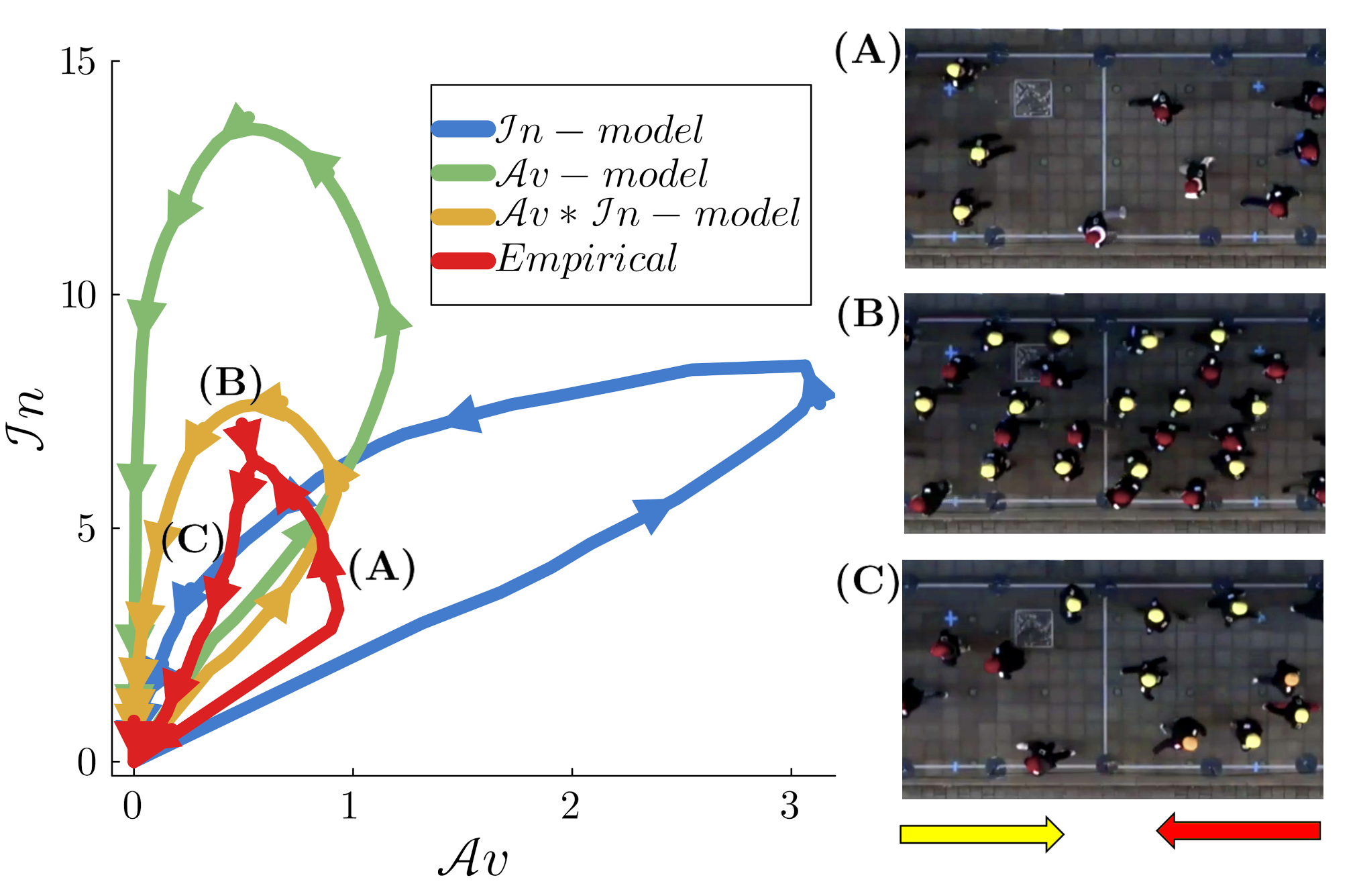
Figure 2: Phase space trajectory during and after the formation of lanes using empirical results [27] and simulations of the proposed models. The arrows in the $\mathcal{I}n-\mathcal{A}v$ plot are spaced by $2.5$ $s$. The temporal values of $\mathcal{A}v$ and $\mathcal{I}n$ are averaged over multiple realizations of the experiment as well as the simulations, with random initial conditions.

The deficiency of models premised solely on $\mathcal{I}n$ or $\mathcal{A}v$ is even more manifest in scenarios which are not confined to the vicinity of the axes of the $(\mathcal{A}v,\mathcal{I}n)$ plane. For example, let us pay attention to the temporal evolution of a bidirectional flow, using as input the experimental data of [27] and averaging over multiple similar realizations. The process of lane formation and then disappearance of the lanes after the two groups have passed each other entails a loop in the phase space, as represented in Fig. 2. Shortly after pedestrians enter the measurement area, in A, the limited space for each crowd leads to moderate values of $\mathcal{I}n$, but $\mathcal{A}v$ gets relatively high as the groups are walking towards each other, until they form lanes in B, thus lowering $\mathcal{A}v$, while $\mathcal{I}n$ is large because space is limited; finally, in C, the crowds have passed each other (low $\mathcal{A}v$) and the pedestrians make use of the available space by dissolving the lanes (moderate $\mathcal{I}n$), marking a return to the origin. Even though all models reproduce the formation of lanes, only the $\mathcal{A}v*\mathcal{I}n$-model produces a loop comparable to the empirical one. While the $\mathcal{I}n$-model is unable to keep in check the growth of $\mathcal{A}v$ prior to lane formation, the $\mathcal{A}v$-model fails to ensure sufficient space between people when lanes have formed, leading to very high $\mathcal{I}n$ values. The dynamics of all scenarios are shown in the video at [37].

While the focus was here put on the asymptotic $\mathcal{I}n$ and $\mathcal{A}v$-models, the discussion has bearing on the broader category of agent-based models: their equations of motion often hinge on variants of either the $\mathcal{I}n_{i}$ variable [38, 39] or the $\mathcal{A}v_{i}$ variable [40, 41, 31], thereby limiting their range of applicability to the associated regime; a detailed inspection of this broader model category is deferred to a future publication.

Finally, in all regimes discussed so far, contacts between pedestrians were at most scarce. The situation is different in the high-$\mathcal{I}n$ region, which is highlighted in red in Fig. 1B and notably includes competitive bottleneck flows; in that case, more realistic (e.g., elliptic) shapes and mechanical contacts should be considered.

In summary, we have shown that the desire to preserve one’s personal space from intrusions and the anticipation of collisions, quantified by the dimensionless numbers $\mathcal{I}n$ and $\mathcal{A}v$, delineate different regimes at the crowd’s scale. These are marked by specific dynamics and ‘structural’ arrangements. The importance of taking into account these factors to model the dynamics of individual agents depends on the regime under study.

At present, only collisions between the hard-cores have been taken into account, in the absence of which ($\mathcal{A}v_{i}=0$), agents are deemed isolated and have thus been left aside in the averaged $\mathcal{A}v$. In reality, the ’softer’ collisions, i.e. the anticipated intrusions into the private or intimate space, are also avoided. A more sophisticated definition of $\mathcal{A}v$ should be able to capture these.

Beyond $\mathcal{I}n$ and $\mathcal{A}v$, other dimensionless numbers can, and certainly should, be introduced to describe specific features of crowd dynamics such as an analogue of the Mach number for the propagation of waves in crowds or some variant of the Péclet number (diffusion over advection) to account for the variability in the outcome of nominally similar experiments, due to the hidden variables $\xi_{i}$ in Eq. 3. Interestingly, such a series of dimensionless numbers would mark successive departures from the conservation laws and invariance principles traditionally encountered in physical systems: While in the $\mathcal{I}n$-regime agents do not differ from particles subjected to distance-based interactions, $\mathcal{A}v$ introduces a velocity-based component to the interactions and a marginal violation of the reciprocity of forces. Better capturing the asymmetry of perception between pedestrians would make the violation of reciprocity more acute, with all its implications in active systems [42]. Eventually, the violation of Galilean invariance in crowds would be mirrored by paying attention not only to TTC, but also to absolute time gaps, should the neighbors suddenly come to a halt. By gradually relaxing the symmetries applicable in physical systems, the way is thus paved for a general theoretical study of the statistical physics of pedestrian assemblies.

Appendix A: Description and curation of the datasets

A large collection of mostly openly available data on pedestrian dynamics has been used in the main text. The collated data and the methods employed to pre-process and extract average dimensionless numbers $\mathcal{I}n$ and $\mathcal{A}v$ from them are detailed in this section.

1 Summary of the datasets

Name	Type	Scenario	Varied Parameter	Details	Cit.	Data
Waiting	Exp.	Static	Density	Jülich, Ger, 2013	-	Supp.
Single-File	Exp.	Single-File	Density	Jülich, Ger, 2006	[23]	[43]
Unidirectional I	Exp.	Uni-dir.	Density	Jülich, Ger, 2013	[25]	[43]
Unidirectional II	Exp.	Uni-dir.	-	Tokyo, Jap, 2018	[26]	[26]
Bidirectional, steady-state	Exp.	Bi-dir.	Density	Jülich, Ger, 2013	[25]	[43]
Bidirectional, pre lane formation	Exp.	Bi-dir.	-	Tokyo, Jap, 2020	[27]	[27]
Zara (Outdoor)	Obs.	Bi-dir.	-	Nicosia, Cy, 2007	[30]	[44]
EWAP (Outdoor)	Obs.	Bi-dir.	-	Zürich, Swi, 2007	[29]	[45]
Cross	Exp.	Multi-dir.	Density	Jülich, Ger, 2013	[25]	[43]
Antipodal	Exp.	Multi-dir.	-	Beijing, PRC, 2019	[28]	-
Students (Outdoor)	Obs.	Multi-dir.	-	Tel Aviv, Isr, 2007	[30]	[44]
Bottleneck	Exp.	Bottleneck	Corr. Width	Jülich, Ger, 2018	[24]	[43]

Table 1: Summary of the different datasets used in our analysis.

Tab. 1 provides a summary of the datasets that have been used, the corresponding references, and, whenever available, download links. Further details about the experimental setups can be found in the references.

Note that, for the Waiting scenario, we had to extract trajectories by ourselves, from existing videos of a controlled experiment conducted within the BasiGo project in $2013$ in Germany. In this experiment, the (27 to 600) participants enter a square area through four entrances. This area is delimited by crowd control barriers and the crowd is filmed from above. After the crowd has entered, the participants wait for approximately one minute before egressing through the entrances. We have extracted parts of this waiting period using the semi-automatic tracking mode of the PeTrack software [46]. The corresponding trajectory data is included as supplemental material.

2 Splitting and merging scenarios

Often, experimental scenarios display different stages and different regions in space. In some cases, specified below, we focused only on part of these stages and regions or we split the data into distinct scenarios.

In most experiments, there is a clear start and end, where the participants start to fill, or begin to leave the measurement area. We will start reporting those experiments, where we analyzed the pseudo-stationary state and overlooked the beginning and end of each run. The Single-File trajectories were treated as purely one-dimensional by neglecting the transverse coordinate. The dataset was split into a dense and a sparse part, where the $6$ runs with the lowest global density are considered as sparse and the rest as dense. In Unidirectional I, we have only used the runs where the width of the entrance and exit corresponds to the total width of the corridor; the other runs rather resemble a bottleneck. As for Unidirectional II, we have used the totally asymmetric runs where all people walk from one side to the other. As there is only a small crowd that passes the measurement area, no steady-state can be analyzed. For simplicity, we have merged the two unidirectional datasets into a Unidirectional scenario. In Bidirectional steady-state, we have used variant $B$, where the participants are instructed to use a fixed exit, i.e. either on the left or on the right at the end of the corridor. For the Cross scenario, we have limited our analysis to the area of the crossing itself. In particular, we have neglected the corridors leading to the crossing area. We have used the variant $A$ of the $90^{\circ}$ crossing, where people enter from all $4$ sides, without an obstacle in the centre of the crossing. Note that, the runs $6$ and $8$, i.e. those with the highest intrusion, where cancelled after some time as the experimenters were afraid that participants could get hurt due to the heavy congestion. We split the Cross dataset in a sparse part consisting of the $3$ runs with the lowest global density and the dense part with the rest. In Bottleneck, only the runs with a number of participants $N>40$ were used. Furthermore we have only used the runs with a high motivation. We restricted the analysis to the area right in front of the bottleneck.

In some experiments, we were interested in transient states, i.e. a specific temporal part of the experiment. In Bidirectional pre lane formation, we have used the runs without any distraction by cellphones, i.e. the baseline condition. We start the measurement after people have entered the measurement area and end it before the lanes have formed. For the Antipodal experiment, only the first $\approx 2$ $s$ of each run are considered. In particular, the part before the pedestrians get close to each other. The runs with a radius of $r=5$ $m$ and $8$ participants were used.

3 The case of the Outdoor scenario (passive observations)

The Outdoor scenario gathers real-world observations from different datasets. The complete sequences have been used. Regarding the Zara and Students datasets, the data are published only in pixel positions and some frames are missing. We have, therefore, used the amended data by [47], where real-world positions were estimated and enhanced by linear interpolation between the frames. Regarding the EWAP datasets, filmed from a Hotel and at the ETH campus, the velocities were given with the positions and frames in two-dimensional real-world units. In contrast to the controlled experiments, many pairs are present in the Outdoor scenario. This has an effect on the structure of the crowd, as we will show in Appendix C. In an atomic vision of the crowd, these pairs (featuring specific ‘intra-molecular’ interactions) must be excluded, for the calculation of $\mathcal{A}v$ and especially $\mathcal{I}n$. To do so, we detect pairs according to a simple rule: Two pedestrians are assumed form a social group if their mean distance is smaller than $1$ $m$, their maximal distance smaller than $1.5$ $m$, and their mutual presence in the scene lasts at least $2$ $s$.

4 Processing and smoothing of trajectories

Unless otherwise specified, in all datasets each pedestrian is assigned a unique ID, for which a two dimensional real-world trajectory is obtained at a certain frame-rate. Although the trajectories were already expressed in real-world coordinates, they featured oscillations due to head sways and empirical noise, which both affect the calculation of $\mathcal{I}n$ and above all $\mathcal{A}v$. To smooth out the head sways, a $4$-th order Butterworth filter with critical frequency $0.5$ Hz was applied to the trajectories. From these positions and times we calculated the velocities as the distance covered in approximately $1$ $s$.

5 Computation of the $\mathcal{I}n$ and $\mathcal{A}v$ numbers and filtering out isolated agents

Subsequently the time-to-collision (TTC) was computed by assuming that each pedestrian is a disk of diameter $\ell=0.2$ $m$. This size was chosen in accordance with [31], in order to limit the number of measured overlaps between disks, which lead to ill-defined TTC and $\mathcal{I}n$ values. Nonetheless, in the very dense experiments, some overlaps are still observed; to mitigate this problem, we set an upper bound $\mathcal{I}n_{ij}^{\text{max}}=400$ and $\mathcal{A}v_{ij}^{\text{max}}=60$ on all computed $\mathcal{I}n$ and $\mathcal{A}v$ numbers.

Besides, despite the segmentations mentioned in Sec. 2, some scenarios (particularly the Outdoor one) remain heteroclite, with a large number of pedestrians that actually walk in isolation. Another example is the sparse Cross scenario, where we want to focus on the half before solving the conflict in the centre of the crossing. Therefore, we exclude pedestrians with $\mathcal{A}v_{i}=0$ in the averaged $\mathcal{A}v$. Excluding these values narrows the datasets down to the parts where interactions really occur and thus yields a much finer and more robust delineation of the different regimes. This is further related to the fact that only collisions between the hard-cores are taken into account. A more sophisticated definition of $\mathcal{A}v$ could capture ’soft’ collisions with the private or intimate space, which were not captured with the discontinuous TTC.

Appendix B: Variations of the Phase Diagram

1 Variations in the definitions of $\mathcal{I}n$ and $\mathcal{A}v$

As we have conceded in the main text, there is a certain freedom in the choice of the definition of $\mathcal{A}v$ and $\mathcal{I}n$. Here, we investigate to what extent this choice impacts the delineation of different regimes.

Let us start with the definition of the Intrusion number $\mathcal{I}n$. For an agent $i$, $\mathcal{I}n$ was defined as the sum of all intrusions over the set $\mathcal{N}_{i}$ of all close neighbors $j$ of $i$, here delimited by $r_{ij}\leqslant 3\,r_{\text{soc}}$. This additivity is similar to the superposition of forces in Physics. However, we are not dealing with forces in the Newtonian sense and the validity superposition is not granted. For instance, it was found to be unreasonable at least in some situations [48]. Therefore, one might choose an alternative neighborhood where the intrusion is dominated by its maximum value as

$$\tilde{\mathcal{I}n}_{i}=\max_{j\neq i}\mathcal{I}n_{ij}.$$ (S6)

The alternative phase diagram is shown in Fig. 3 (a). It is difficult to spot any substantial difference to the original diagram: the delineation is robust under this change. In an analogous way, for the Avoidance number, we can replace the maximum with a sum. In that case, the delineation of different regimes gets blurred to a large extent. On the other hand, if more weight is put on the large Avoidance numbers by defining it symmetrically to the Intrusion number, viz.,

$$\tilde{\mathcal{A}v}_{i}=\sum_{j\neq i}\left(\frac{\tau_{0}}{\tau_{ij}}\right)^{2},$$ (S7)

the delineation is at least partly recovered, see Fig. 3 (b).

2 Use of the density instead of $\mathcal{I}n$

We chose to base the Intrusion number on distances instead of using the local density. This is partly justified by the ambiguity in the definition of a local density. However, we acknowledge that the averaged $\mathcal{I}n$ is still closely related to the density, which certainly is the quantity most commonly used to classify crowds.

In Fig. 3 (c), we have substituted the Intrusion number with the global density $\rho$, calculated as the number of pedestrians divided by the available space.

To enable us to plot the Single-File data along with the rest, the one-dimensional density, calculated as the number of people divided by the length of the track, was rescaled according to [49], where we assumed a width of $0.3$ $m$. The delineation of different regimes is still clearly visible. Only the Single-File data strongly deviates from the original diagram. In particular, relative to the rest of the diagram, moderate intrusions seem to correspond to high densities. In the Single-file scenario, the pedestrians do not have neighbors to the sides. Therefore, the deviation might actually be reflected in the subjective feeling of the pedestrians. On the other hand, the deviation could also be explained by the presence of obstacles, e.g. walls, which are very close to all of the agents in the single-file scenario and have not been taken into account.

Besides, the Cross scenario and the Bottleneck scenario are at lower densities, but higher $\mathcal{I}n$, compared to the Waiting scenario. In the latter people are distributed very homogeneously, whereas inhomogeneities are conspicuous in the former, including regions of tight packing. The Intrusion number puts more weight on these.

(a) $\max\left(\mathcal{I}n\right)$

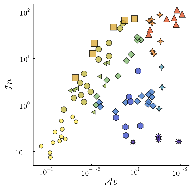
(b) $\sum(\tau_{0}/\tau)^{2}$

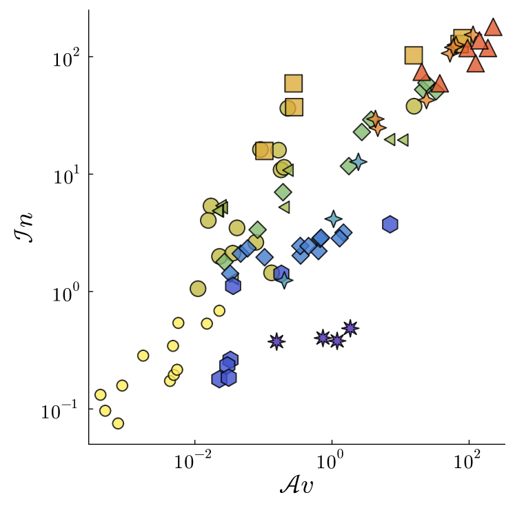
(c) Density

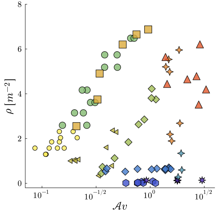
Figure 3: Empirical delineation of different regimes with alternative definitions of the Avoidance number $\mathcal{A}v$ and the Intrusion number $\mathcal{I}n$ (or the global density).

3 Effect of correlations between the empirical values of $\mathcal{I}n$ and $\mathcal{A}v$

There may be some correlation between $\mathcal{I}n$ and $\mathcal{A}v$, so that when one of them changes, the other changes as well. The systematic increase in $\mathcal{A}v$ in unidirectional flows as the crowd gets denser, even after application of the Butterworth filter to correct head sway, supports this impression. In the main text, we have seen that $\mathcal{I}n$ and $\mathcal{A}v$ are sufficiently independent to allow for a proper distinction between the typical scenarios encountered in pedestrian streams. In any case, even some degree of interdependence would mostly result in a skewed diagram (given that the $\mathcal{I}n$ and $\mathcal{A}v$ axes have been plotted orthogonally although they should not) with no impact on its topology.

Appendix C: Structure of Crowds

We have used the pair-distribution function (pdf) to probe the structure of crowds and, subsequently, to identify the best descriptor of its self-organized structure. Here, we give more details on the calculation of the pdf. Then we will investigate the structure of crowds in different scenarios in more detail.

1 Definition of the observable

The pdf is generally used to infer the atomic or molecular structure of materials. An illustration of the relation of the pdf to the structure of a material is shown in Fig. 4; an experimental example of a pdf, measured for solid and liquid Argon, can for example be found in [50]. In our case, we calculate the pdf of crowds according to [31]. For some variable $x$ the pdf is given by the probability that two pedestrians are separated by $x$ normalized by the probability $P_{\text{NI}}(x)$ that two non-interacting pedestrians are separated by $x$, in particular $g(x)=P(x)/P_{\text{NI}}(x)$. This normalization is aimed at correcting the lack of translational invariance in crowd observations.

While $P(x)$ can be simply estimated by the relative frequencies in the dataset, $P_{\text{NI}}(x)$ is in principle unknown. However, it can be estimated by randomizing either the spatial or the temporal information. To estimate the distribution, we used strict binning with bins of size $0.1$ $m$ or $0.1$ $s$.

2 Interpretation in various scenarios

This procedure is best understood in the case of single-file motion. Here, the observational area is limited to the $x$-coordinate and ranges from $0$ to $L$. As all pedestrians enter the scene on the left and leave on the right, all positions are equally likely. However, due to the limited size of the area, finite-size effects strongly suppress large distances. Therefore we can estimate $P_{\text{NI}}(x)$ by calculating the distribution of distances between points that are randomly positioned on the interval $[0,L]$. Another way to estimate $P_{\text{NI}}(x)$ is by randomzing the time-information, i.e. by creating a ’time-scrambled’ version of the dataset as proposed by [31]. This ensures that the distances calculated in the scrambled dataset correspond to non-interacting pedestrians as they have not been in the same frame originally. Both procedures lead to the same result in the case of single-file motion.

In the case of the static crowd, the scrambling of temporal information cannot be employed, as the pedestrians are hardly moving. Therefore, we assume that all positions within the rectangle are equally likely. As we neglect the edges of the observational area, where people lean on the crowd-control barrier, this assumption is justified.

In the Outdoor dataset, alongside finite-size effects, one has to account for different forbidden areas (like trees or cars) in the middle of the scenes and the different areas where people tend to enter or leave the scene. This is achived by randomizing the time-information.

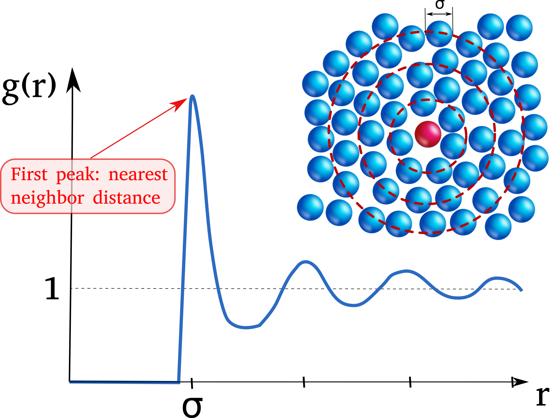
Figure 4: Exemplary figure of the pair-distribution function

(a) Corridor

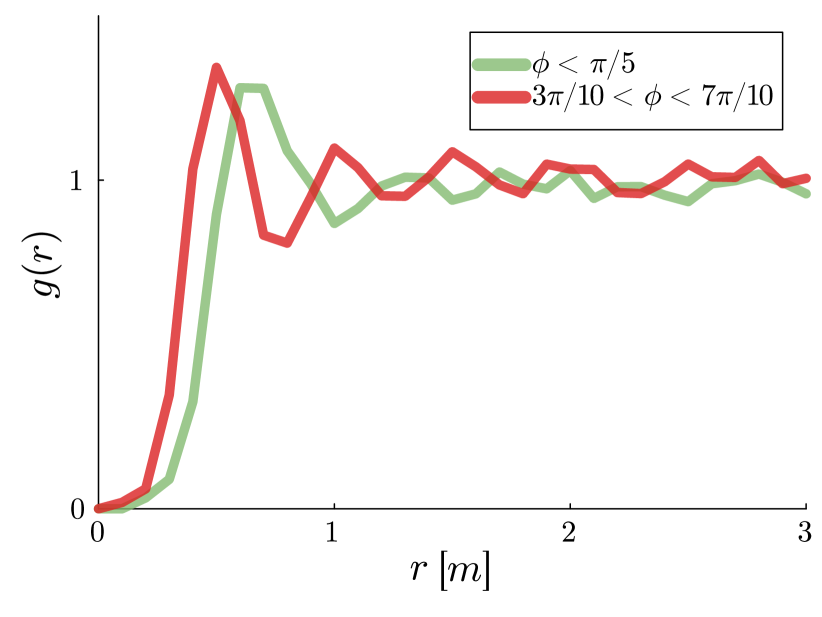
(b) Outdoor

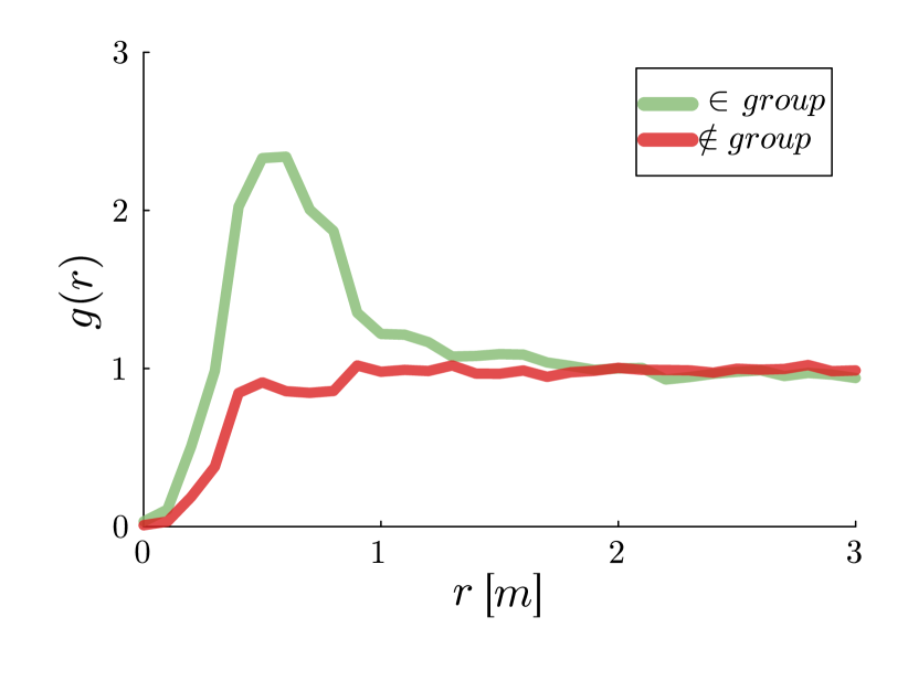
(c) Outdoor

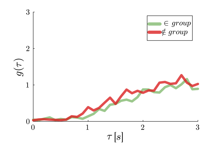
Figure 5: Evaluation of the pdf $g(r)$ in different scenarios. In (a), i.e. the Unidirectional I dataset, the run with $\rho=2.1/m^{2}$ the position of the peaks depends on the angle $\phi$. In particular, the longitudal distances (to the front) are larger than the transversal distances (to the sides). In (b), the Outdoor dataset, the marked peak at small distances to the sides arises from many pairs which are present in the observation. This cannot be observed in the TTC-based pdf $g(\tau)$, cf. (c).

3 Insight given by the pdf into the crowd’s structure in different scenarios

Probably the most confined and homogeneous pedestrian experiments were conducted by [23]: high density, periodic, single-file experiments with soldiers as the participants. The corresponding pdf is shown in Fig. 1 (C) in the main text for a single run at $\rho=2.1/m$, where long-ranged correlations in the pdf can be seen, owing to the strong homogeneity, combined with the spatially confined setting. The pdf displays peaks that are well separated and located at the integral multiples of the mean spacing, i.e. correspond to the $k$-th neighbor.

Let us now turn to the unidirectional flow through a corridor with open boundaries at a density of $\rho=2.1/m^{2}$. The corresponding pdf is shown in Fig. 5 (a). Multiple peaks are still visible but the correlation length is much smaller. The two curves exhibit a difference between transversal (green) and longitudinal (red) distances, reflecting the existence of anisotropy. In particular, pedestrians keep smaller distances to their sides than to the front. The angular dependence may have practical implications as to whether the capacity of a corridor increases linearly or step-wise with its width.

4 Effect of pairs and social groups on the pdf

Finally, we have calculated the pdf for the Outdoor dataset. As earlier, we have identified pairs according to a simple classification. Very distinct curves are seen in Fig. 5 (b), depending on whether pedestrian $i$ is part of a social group ($\in group$) or not ($\notin group$). Pedestrians that form a social group want to interact (e.g. talk) and, therefore, stay in each other’s personal space, generally walking abreast. This attractive interaction leads to a strong peak at small (transversal) distances. Apart from this and a strong short-ranged repulsion, no spatial structure can be seen. The pdf bears resemblance to a mixed gas consisting of single atoms and molecules. If the pdf is calculated for the time-to-collision, cf. Fig. 5 (c), the two curves collapse onto each other, because proximity in space is not associated with a risk of imminent collision: Pair members want to stay relatively close to each other but do not want to collide. The main text has underlined that the finding of [31] (namely, that the TTC is a more suitable descriptor than the spatial distances) is valid in a certain regime only (i.e. low $\mathcal{I}n$, moderate $\mathcal{A}v$).

By turning the original argument upside down, we contend that further restrictions are necessary when it comes to social groups: distance-based (‘proxemic’) interactions within each group are combined with TTC-based (avoidance) interactions with other people. These two levels are reflected in their corresponding pdf: the peak at short distances in $g(r)$ (but not in $g(\tau)$) is only present for members of social groups. Incidentally, this also explains the large variations in the pdf $g(r)$ in [31], binned by rates of approach: in [31], pairs were not excluded and the rate of approach of their members is very small, and thus falls in one specific bin.

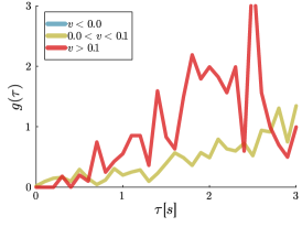
Figure 6: The pair-distribution function $g(\tau)$ for the Waiting dataset binned according to different rates of approach $v$.

5 Waiting scenario

In Fig. 6 we show that for the Waiting dataset the curves of $g(\tau)$ do not collapse onto each other if binned according to the rate of approach $v$. For negative rates of approach (hence, infinite TTC), no curve can be plotted in Fig. 6 even though the structure is independent of it in real space (Fig. 1 (D), in the main text).

The failure of $g(\tau)$ to describe the dynamics in the high $\mathcal{I}n$ and low $\mathcal{A}v$ regime has bearing on the modeling of starting waves, see e.g. [51, 52]. Indeed, whether the pedestrians ahead of a reference agent stand still ($v\approx 0$) or move ahead ($v<0$), their TTC is infinite, so that a purely TTC (or $\mathcal{A}v$)-based model will not reproduce the backward-propagating starting wave that is observed in reality [1].

Appendix D: Perturbative Analysis

In this Appendix, we detail the perturbative expansion that gives rise to the proposed $\mathcal{I}n$, $\mathcal{A}v$ and $\mathcal{A}v*\mathcal{I}n$-models. For the implementations, the code of the models is available at [53].

1 Generic cost function

Consider $N$ circular agents of diameter $\ell$. The position of agent $i$ is $\bm{r}_{i}(t)=\left(x_{i}(t),y_{i}(t)\right)$, $\bm{v}_{i}=\dot{\bm{r}}_{i}(t)$ the velocity, $\bm{a}_{i}=\ddot{\bm{r}}_{i}(t)$ the acceleration, and $\bm{v}_{\text{des},i}$ the desired velocity. Let $\mathcal{R}(t)=\left(\bm{r}_{1}(t),\dots,\bm{r}_{N}(t)\right)$ denote the set of all positions at time $t$ and $\mathcal{V}(t)=\left(\bm{v}_{1}(t),\dots,\bm{v}_{N}(t)\right)$ the set of all velocities.

We have argued that, in most scenarios, the way in which pedestrians choose their velocity can be approximated by

$$\bm{v}_{i}^{\star}=\underset{\bm{v}\in\mathbb{R}^{2}}{\text{arg min}}\,\mathcal{C}_{i}\left[\bm{v},\mathcal{I}n_{i}(\bm{r}),\mathcal{A}v_{i}\left(\bm{v}\right)\right],$$ (S8)

where we shortened the dependencies $\mathcal{A}v_{i}\left(\bm{v}\right)=\mathcal{A}v_{i}\left(\bm{v},\mathcal{R}(t),\mathcal{V}(t)\right)$ and $\mathcal{I}n_{i}(\bm{r})=\mathcal{I}n_{i}\left(\bm{r}_{i}(t)+\bm{v}\delta t,\mathcal{R}(t)\right)$. Recall that $\bm{v}$ denotes the test-velocity and $\bm{r}=\bm{r}_{i}(t)+\bm{v}\delta t$ the associated test position.

Expanding the cost-function of Eq. S8 to the lowest order in $\mathcal{I}n_{i}$ and $\mathcal{A}v_{i}$, notably, around the non-interacting situation, yields

$$C_{i}\left[\bm{v},\mathcal{I}n_{i}\left(\bm{r}\right),\mathcal{A}v_{i}\left(\bm{v}\right)\right]\approx C_{i}^{(0)}\left(\bm{v}\right)+a_{i}\,\mathcal{A}v_{i}\left(\bm{v}\right)+b_{i}\,\mathcal{I}n_{i}\left(\bm{r}\right),$$ (S9)

where we have introduced $C_{i}^{(0)}\left(\bm{v}\right)=C_{i}\left(\bm{v},\mathcal{A}v_{i}=0,\mathcal{I}n_{i}=0\right)$ and the constants $a_{i}=\partial C_{i}/\partial\mathcal{A}v_{i}|_{\mathcal{A}v_{i}=0}$, and $b_{i}=\partial C_{i}/\partial\mathcal{I}n_{i}|_{\mathcal{I}n_{i}=0}$. In the following, we will look at asymptotic scenarios to further simplify Eq. S9.

2 Reference situation: The isolated agent

Let us start with the simplest case, namely an isolated pedestrian, i.e. $\mathcal{I}n_{i}=0$ and $\mathcal{A}v_{i}=0$. Equation S9, the model then reduces to

$$\bm{v}_{i}^{\star}=\underset{\bm{v}\in\mathbb{R}^{2}}{\arg\min}\,C_{i}^{(0)}\left(\bm{v}\right)$$ (S10)

This minimum is reached for $\bm{v}_{i}^{\star}=\bm{v}_{\text{des},i}$ for the freely walking pedestrian, so

$$\bm{0}=\nabla_{\bm{v}}\,C_{i}^{(0)}\left(\bm{v}\right)\Big{|}_{\bm{v}=\bm{v}_{\text{des},i}},$$ (S11)

where $\nabla_{\bm{v}}=\left(\partial/\partial v_{x_{i}},\partial/\partial v_{y_{i}}\right)$, and the Hessian matrix $\underline{M}=\partial^{2}C_{i}^{(0)}\left(\bm{v}\right)/\partial\bm{v}^{2}|_{\bm{v}=\bm{v}_{\text{des},i}}$ is positive definite. In the following we will make an assumption of isotropy around the optimal velocity, in which case $\underline{M}$ is an identity matrix multiplied by a positive scalar $\gamma_{i}$. Then, up to second order, the cost-function for an isolated pedestrian is

$$C_{i}^{(0)}\left(\bm{v}\right)=\gamma_{i}\left(\bm{v}_{\text{des},i}-\bm{v}\right)^{2}.$$ (S12)

Here, we omit the positional dependence of the desired velocity. The cost increases as the squared Euclidean distance between the test velocity and the desired velocity. In particular, deviations in the magnitude and the direction of the desired velocity are similarly penalized. While a common assumption the literature, this need not be exact in reality.

3 The $\mathcal{A}v$-model

Let us now turn to a scenario in which $\mathcal{I}n_{i}=0$ and $\mathcal{A}v_{i}\neq 0$, for example two joggers that are still well separated but face an anticipated collision. In this case, the cost-function Eq. S9, together with the considerations above, simplifies to

$$C_{i}\left[\bm{v},\mathcal{A}v_{i}\left(\bm{v}\right)\right]\approx\mathcal{A}v_{i}\left(\bm{v}\right)+\frac{1}{\alpha_{i}}\left(\bm{v}_{\text{des},i}-\bm{v}\right)^{2},$$ (S13)

Here, we introduced $\alpha_{i}=a_{i}/\gamma_{i}$ and rescaled the cost-function by the constant $a_{i}$. Complemented with relaxation process, where the actual velocity relaxes towards $\bm{v}_{i}^{\star}$ as $\bm{a}_{i}=\left(\bm{v}_{i}^{\star}-\bm{v}_{i}(t)\right)/\tau_{R}$, we recover the proposed $\mathcal{A}v$-model.

4 The $\mathcal{I}n$-model

Now, we assume the case $\mathcal{I}n_{i}\neq 0$ and $\mathcal{A}v_{i}=0$, for example in a moderately dense, static crowd. The perturbative ansatz yields

$$C_{i}\left[\bm{v},\mathcal{I}n_{i}\left(\bm{r}\right)\right]\approx\gamma_{i}\left(\bm{v}_{\text{des},i}-\bm{v}\right)^{2}+b_{i}\,\mathcal{I}n_{i}\left(\bm{r}\right).$$ (S14)

If we look at the condition for $\bm{v}_{i}^{\star}$ as

$$\bm{0}=\gamma_{i}\,\nabla_{\bm{v}}\left(\bm{v}_{\text{des},i}-\bm{v}\right)^{2}\big{|}_{\bm{v}=\bm{v}_{i}^{\star}}+b_{i}\,\nabla_{v}\mathcal{I}n_{i}\left(\bm{r}\right)\big{|}_{\bm{r}=\bm{r}_{i}(t)+\bm{v}_{i}^{\star}}.$$ (S15)

We can make a substitution as

$$\bm{0}=-2\gamma_{i}\left(\bm{v}_{\text{des},i}-\bm{v}_{i}^{\star}\right)+b_{i}\delta t\,\nabla_{r}\mathcal{I}n_{i}\left(\bm{r}\right)\big{|}_{\bm{r}=\bm{r}_{i}(t)+\bm{v}_{i}^{\star}\delta t},$$ (S16)

where $\nabla_{r}=\left(\partial/\partial x_{i},\partial/\partial y_{i}\right)$. For small $\delta t$, one can assume $\bm{r}\approx\bm{r}_{i}(t)$ and subsequently obtain a model as

$$\bm{v}_{i}^{\star}=\bm{v}_{\text{des},i}-\beta_{i}\cdot\nabla_{r}\mathcal{I}n_{i}\left(\bm{r}_{i}(t)\right),$$ (S17)

where we introduced $\beta_{i}=b_{i}\delta t$. Eq. S17, if combined with a relaxation time-scale, the proposed $\mathcal{I}n$-model.

5 The $\mathcal{A}v*\mathcal{I}n$-model

Let us know turn to the general case $\mathcal{A}v_{i},\mathcal{I}n_{i}\neq 0$. The extremal condition for $\bm{v}_{i}^{\star}$ reads

$$\bm{0}=\nabla_{\bm{v}}\underset{C^{(\mathcal{I}n)}_{i}}{\underbrace{\left[\gamma_{i}\cdot\left(\bm{v}_{\text{des},i}-\bm{v}\right)^{2}\big{|}_{\bm{v}=\bm{v}_{i}^{\star}}+b_{i}\cdot\mathcal{I}n_{i}\left(\bm{r}\right)\big{|}_{\bm{r}=\bm{r}_{i}(t)+\bm{v}_{i}^{\star}\delta t}\right]}}+a_{i}\cdot\nabla_{\bm{v}}\mathcal{A}v_{i}\left(\bm{v}\right)\big{|}_{\bm{v}=\bm{v}_{i}^{\star}}.$$ (S18)

where the gradient of $C^{(\mathcal{I}n)}_{i}$ can be expanded around the solution of the $\mathcal{I}n$-model (Eq. S17), i.e., $\bm{v}^{(\mathcal{I}n)}=\bm{v}_{\text{des},i}-\beta_{i}\,\nabla_{\bm{r}}\mathcal{I}n_{i}\left(\bm{r}_{i}(t)\right)$, as follows

$$\nabla_{v}C^{(\mathcal{I}n)}_{i}\big{|}_{\bm{v}=\bm{v}_{i}^{\star}}\approx\underset{=0}{\underbrace{\nabla_{v}C^{(\mathcal{I}n)}_{i}\big{|}_{\bm{v}=\bm{v}_{i}^{(\mathcal{I}n)}}}}+\nabla^{2}_{v}C^{(\mathcal{I}n)}_{i}\big{|}_{\bm{v}=\bm{v}_{i}^{(\mathcal{I}n)}}\left(\bm{v}^{\star}_{i}-\bm{v}^{(\mathcal{I}n)}_{i}\right)\approx 2\gamma_{i}\left(\bm{v}^{\star}_{i}-\bm{v}^{(\mathcal{I}n)}_{i}\right).$$ (S19)

Now, by plugging Eq. S19 into Eq. S18, and integrating, one obtains

$$C_{i}\left[\bm{v},\mathcal{I}n_{i}\left(\bm{r}\right),\mathcal{A}v_{i}\left(\bm{v}\right)\right]\approx\mathcal{A}v_{i}\left(\bm{v}\right)+\frac{1}{\alpha_{i}}\left[\bm{v}_{\text{des},i}-\beta_{i}\cdot\nabla_{r}\mathcal{I}n_{i}\left(\bm{r}_{i}(t)\right)-\bm{v}\right]^{2},$$ (S20)

which is the cost-function of the $\mathcal{A}v*\mathcal{I}n$-model.

Appendix E: Connection between the dynamics and the structure

In the main text, we have delineated asymptotic regimes ($\mathcal{A}v\to 0$ or $\mathcal{I}n\to 0$) in the dynamics of crowd flows, in which the microscopic dynamics of each agent are governed by only the intrusion variable $\mathcal{I}n_{i}$ or the avoidance variable $\mathcal{A}v_{i}$. Empirical evidence has revealed distinct types of crowd arrangement in these two regimes, characterised by the pdf $g(r)$ and $g(\tau)$, respectively.

Theoretically, it is thus tempting to prove that, if, say, the dynamics hinge on the distance-based variable $\mathcal{I}n_{i}$, independently of the TTC, then the crowd’s structure will be characterised by a pdf $g(r)$ that is independent of other variables such as the rate of approach $v$. While this is of course true if an equilibrium state is reached in which the separations between particles are a function of a potential that only depends on the intrusion variable (hence $r$), it so happens that it does not hold systematically.

Indeed, as an assembly of agents in the $\mathcal{A}v\to 0$ regime evolves, starting from a well-mixed configuration, the pdf $g(r)$ may develop a dependence on $v$ even if the interactions between agents are only a function of $r$.

To illustrate this point, we consider a minimal model in which two particles of mass $m=1$, $j=1$ and $j=2$, move on a one-dimensional line, obeying Newtonian dynamics with a distance-based interaction potential $\mathcal{V}(r)=r^{-2}$, where $r=r_{2}-r_{1}$ ($r_{2}>r_{1}$), viz.,

$$m\ddot{r}_{j}=-\frac{d\mathcal{V}}{dr_{j}}(r_{j}).$$ (S21)

The spacing $r$ obeys

$$\frac{1}{2}m\ddot{r}=-\frac{d\mathcal{V}}{dr}(r).$$ (S22)

Starting from a configuration with $r$ and $v=\dot{r}_{2}-\dot{r}_{1}$ randomly sampled from a uniform distribution on a large interval, Eq. S22 is solved numerically. Noticing that for non-interacting particles one simply has $r=r(t=0)+v(t=0)\,t$, the renormalized pdf $g(r,t)$, shown in Fig. 7 at different times $t$, while initially independent of the rate of approach $v$ (independent of whether $v<0$ or $v\leqslant 0$, develop a dependence on $v$ near $r\approx 0$ as time goes on. This is easily explained: the strong repulsive interactions when $r\to 0$ quickly turn the particles away from one another, thus making $v$ negative. Therefore, there are but few realizations with small $r$ and $v>0$. More generally, the origin of the dependence of the pdf on the rate of approach $v$ is that, while the interactions depend on $r$ and not on $v$, they causally affect $v$, thus possibly introducing correlations between spacings and rates of approach.

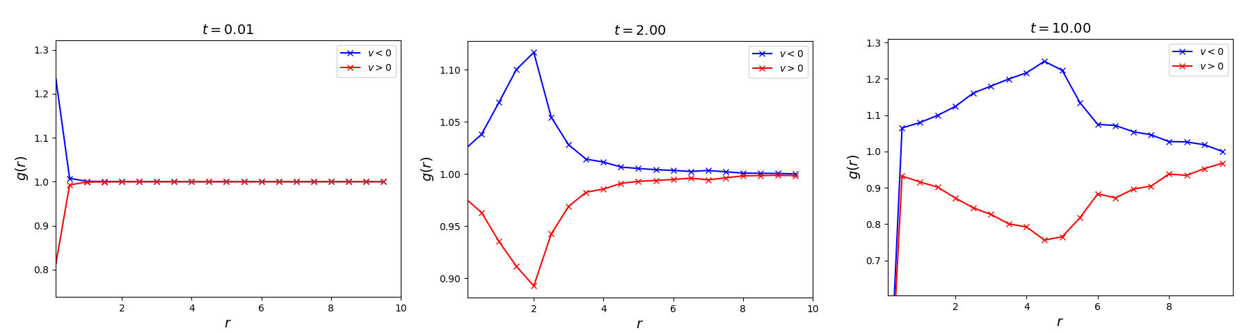
Figure 7: Evolution of the pdf $g(r,t)$, binned by rate of approach $v$ ($v<0$ or $v\geqslant 0$), with time $t$ in a minimal one-dimensional model in which two Newtonian particles interact with a purely distance-based potential.

References

- Bain and Bartolo [2019] N. Bain and D. Bartolo, Dynamic response and hydrodynamics of polarized crowds, Science 363, 46 (2019).
- Hugo [1872] V. Hugo, L’Année terrible / Les 7,500,000 oui (Michel Lévy, frères, 1872).
- Henderson [1974] L. F. Henderson, On the fluid mechanics of human crowd motion, Transportation research 8, 509 (1974).
- Hughes [2003] R. L. Hughes, The flow of human crowds, Annual Review of Fluid Mechanics 35, 169 (2003).
- Martinez-Gil et al. [2017] F. Martinez-Gil, M. Lozano, I. Garcia-Fernandez, and F. Fernandez, Modeling, evaluation, and scale on artificial pedestrians: a literature review, ACM Computing Surveys (CSUR) 50, 72 (2017).
- Schadschneider et al. [2018] A. Schadschneider, M. Chraibi, A. Seyfried, A. Tordeux, and J. Zhang, Pedestrian dynamics: From empirical results to modeling, Crowd Dynamics, Volume 1: Theory, Models, and Safety Problems 1, 63 (2018).
- Chraibi et al. [2018] M. Chraibi, A. Tordeux, A. Schadschneider, and A. Seyfried, Modelling of pedestrian and evacuation dynamics, Encyclopedia of Complexity and Systems Science https://doi.org/10.1007/978-3-642-27737-5_705-1 (2018).
- Maury and Faure [2018] B. Maury and S. Faure, Crowds in Equations: An Introduction to the Microscopic Modeling of Crowds (2018).
- Fruin [1971] J. Fruin, Pedestrian Planning and Design (Metropolitan Association of Urban Designers and Environmental Planners, New York, 1971).
- Schadschneider et al. [2010] A. Schadschneider, D. Chowdhury, and K. Nishinari, Stochastic Transport in Complex Systems: From Molecules to Vehicles (Elsevier, 2010).
- Best et al. [2014] A. Best, S. Narang, S. Curtis, and D. Manocha, DenseSense: Interactive Crowd Simulation using Density-Dependent Filters (2014).
- Feliciani et al. [2021] C. Feliciani, K. Shimura, and K. Nishinari, Introduction to Crowd Management (Springer, Cham, Switzerland, 2021).
- Zanlungo et al. [2023] F. Zanlungo, C. Feliciani, Z. Yücel, X. Jia, K. Nishinari, and T. Kanda, A pure number to assess “congestion” in pedestrian crowds, Transportation Research Part C: Emerging Technologies 148, 104041 (2023).
- Hayduk [1978] L. A. Hayduk, Personal space: An evaluative and orienting overview, Psychological Bulletin 85, 117 (1978).
- Evans and Wener [2007] G. W. Evans and R. E. Wener, Crowding and personal space invasion on the train: Please don’t make me sit in the middle, Journal of Environmental Psychology 27, 90 (2007).
- Lian et al. [2018] L. Lian, W. Song, K. K. R. Yuen, and L. Telesca, Analysis of repulsion states among pedestrians inflowing into a room, Physics Letters A 382, 2424 (2018).
- Knowles et al. [1976] E. S. Knowles, B. Kreuser, S. Haas, M. Hyde, and G. E. Schuchart, Group size and the extension of social space boundaries, Journal of Personality and Social Psychology 33, 647 (1976).
- Jia et al. [2022] X. Jia, C. Feliciani, H. Murakami, A. Nagahama, D. Yanagisawa, and K. Nishinari, Revisiting the level-of-service framework for pedestrian comfortability: velocity depicts more accurate perceived congestion than local density, Transportation Research Part F: Traffic Psychology and Behaviour 87, 403 (2022).
- Delucia and Novak [1997] P. R. Delucia and J. B. Novak, Judgments of relative time-to-contact of more than two approaching objects: Toward a method, Perception & Psychophysics 59, 913 (1997).
- Lee [1976] D. N. Lee, A Theory of Visual Control of Braking Based on Information about Time-to-Collision, Perception 5, 437 (1976).
- Pfaff and Cinelli [2018] L. M. Pfaff and M. E. Cinelli, Avoidance behaviours of young adults during a head-on collision course with an approaching person, Experimental Brain Research 236, 3169 (2018).
- Meerhoff et al. [2018] L. A. Meerhoff, J. Bruneau, A. Vu, A.-H. Olivier, and J. Pettré, Guided by gaze: Prioritization strategy when navigating through a virtual crowd can be assessed through gaze activity, Acta psychologica 190, 248 (2018).
- Seyfried et al. [2010] A. Seyfried, A. Portz, and A. Schadschneider, Phase Coexistence in Congested States of Pedestrian Dynamics, in Cellular Automata, Vol. 6350, edited by S. Bandini, S. Manzoni, H. Umeo, and G. Vizzari (Springer Berlin Heidelberg, Berlin, Heidelberg, 2010) pp. 496–505.
- Adrian et al. [2020] J. Adrian, A. Seyfried, and A. Sieben, Crowds in front of bottlenecks at entrances from the perspective of physics and social psychology, Journal of The Royal Society Interface 17, 20190871 (2020).
- Cao et al. [2017] S. Cao, A. Seyfried, J. Zhang, S. Holl, and W. Song, Fundamental diagrams for multidirectional pedestrian flows, Journal of Statistical Mechanics: Theory and Experiment 2017, 033404 (2017).
- Feliciani et al. [2018] C. Feliciani, H. Murakami, and K. Nishinari, A universal function for capacity of bidirectional pedestrian streams: Filling the gaps in the literature, PLOS ONE 13, e0208496 (2018).
- Murakami et al. [2021] H. Murakami, C. Feliciani, Y. Nishiyama, and K. Nishinari, Mutual anticipation can contribute to self-organization in human crowds, Science Advances 7, eabe7758 (2021).
- Xiao et al. [2019] Y. Xiao, Z. Gao, R. Jiang, X. Li, Y. Qu, and Q. Huang, Investigation of pedestrian dynamics in circle antipode experiments: Analysis and model evaluation with macroscopic indexes, Transportation Research Part C: Emerging Technologies 103, 174 (2019).
- Pellegrini et al. [2009] S. Pellegrini, A. Ess, K. Schindler, and L. van Gool, You’ll never walk alone: Modeling social behavior for multi-target tracking, in 2009 IEEE 12th International Conference on Computer Vision (2009) pp. 261–268.
- Lerner et al. [2007] A. Lerner, Y. Chrysanthou, and D. Lischinski, Crowds by Example, Computer Graphics Forum 26, 655 (2007).
- Karamouzas et al. [2014] I. Karamouzas, B. Skinner, and S. J. Guy, A universal power law governing pedestrian interactions, Phys. Rev. Lett. 113, 238701 (2014).
- Klongvessa [2020] N. Klongvessa, Study of Dense Assemblies of Active Colloids: collective Behavior and Rheological Properties, Ph.D. thesis, Université de Lyon (2020).
- van Toll et al. [2020] W. van Toll, F. Grzeskowiak, A. L. Gandía, J. Amirian, F. Berton, J. Bruneau, B. C. Daniel, A. Jovane, and J. Pettré, Generalized Microscropic Crowd Simulation using Costs in Velocity Space, in Symposium on Interactive 3D Graphics and Games (ACM, San Francisco CA USA, 2020) pp. 1–9.
- Hoogendoorn and Bovy [2003] S. Hoogendoorn and P. Bovy, Simulation of pedestrian flows by optimal control and differential games, Optim. Control Appl. Meth. 24, 153 (2003).
- Guy et al. [2012] S. J. Guy, S. Curtis, M. C. Lin, and D. Manocha, Least-effort trajectories lead to emergent crowd behaviors, Physical Review E 85, 016110 (2012).
- Note [1] We have chosen homogeneous parameters for all simulations: , , , , and . Furthermore, we have introduced a social radius for the -part of the model to account for the fact that people do not only avoid collisions between the hard-cores of size . Besides, a small scalar is subtracted from in Eq. 1 to make continuous across the cut-off radius.
- [37] Supplemental videos, https://youtu.be/E8NvgRLPvLg.
- Helbing et al. [2000] D. Helbing, I. Farkas, and T. Vicsek, Simulating dynamical features of escape panic, Nature 407, 487 (2000).
- Tordeux et al. [2016] A. Tordeux, M. Chraibi, and A. Seyfried, Collision-Free Speed Model for Pedestrian Dynamics, in Traffic and Granular Flow ’15, edited by V. L. Knoop and W. Daamen (Springer International Publishing, Cham, 2016) pp. 225–232.
- van den Berg et al. [2008] J. van den Berg, M. Lin, and D. Manocha, Reciprocal Velocity Obstacles for Real-Time Multi-Agent Navigation, in Robotics and Automation, 2008. ICRA 2008. IEEE International Conference On (2008 IEEE International Conference on Robotics and Automation Pasadena, CA, USA, May 19-23, 2008, 2008).
- van den Berg et al. [2011] J. van den Berg, S. Guy, M. Lin, and D. Manocha, Reciprocal n-Body Collision Avoidance, in Springer Tracts in Advanced Robotics, Vol. 70 (2011) pp. 3–19.
- Fruchart et al. [2021] M. Fruchart, R. Hanai, P. B. Littlewood, and V. Vitelli, Non-reciprocal phase transitions, Nature 592, 363 (2021).
- [43] Database Jülich, https://doi.org/10.34735/ped.da.
- _Ob [a] Observations I, graphics.cs.ucy.ac.cy/research/downloads/crowd-data (a).
- _Ob [b] Observations II, http://www.vision.ee.ethz.ch/datasets/ (b).
- Boltes et al. [2010] M. Boltes, A. Seyfried, B. Steffen, and A. Schadschneider, Automatic extraction of pedestrian trajectories from video recordings, in Pedestrian and Evacuation Dynamics 2008, edited by W. W. F. Klingsch, C. Rogsch, A. Schadschneider, and M. Schreckenberg (Springer, Berlin Heidelberg, 2010) pp. 43–54.
- Alahi et al. [2016] A. Alahi, K. Goel, V. Ramanathan, A. Robicquet, L. Fei-Fei, and S. Savarese, Social LSTM: Human Trajectory Prediction in Crowded Spaces, IEEE Conference on Computer Vision and Pattern Recognition (CVPR) (2016).
- Seyfried [2018] A. Seyfried, Intentions and superposition of forces in pedestrian models, presentation at PED 2018, Lund, Sweden (2018).
- Seyfried et al. [2005] A. Seyfried, B. Steffen, W. Klingsch, and M. Boltes, The fundamental diagram of pedestrian movement revisited, J. Stat. Mech. P10002, 10.1088/1742-5468/2005/10/P10002 (2005).
- Franchetti [1975] S. Franchetti, Radial distribution functions in solid and liquid argon, Il Nuovo Cimento B (1971-1996) 26, 507 (1975).
- Tomoeda et al. [2012] A. Tomoeda, D. Yanagisawa, T. Imamura, and K. Nishinari, Propagation speed of a starting wave in a queue of pedestrians, Physical Review E 86, 036113 (2012).
- Rogsch [2010] C. Rogsch, Start Waves and Pedestrian Movement— An Experimental Study, in Pedestrian and Evacuation Dynamics 2008, edited by W. W. F. Klingsch, C. Rogsch, A. Schadschneider, and M. Schreckenberg (Springer Berlin Heidelberg, Berlin, Heidelberg, 2010) pp. 247–248.
- [53] Modelling Framework, https://github.com/Jakob-KKU/Pedestrian_Models.