Propagation of carbon taxes in credit portfolio through macroeconomic factors

Abstract

We study how the introduction of carbon taxes in a closed economy propagate in a credit portfolio and precisely describe how carbon taxes dynamics affect the firm value and credit risk measures such as probability of default, expected and unexpected losses. We adapt a stochastic multisectoral model to take into account carbon taxes on both sectoral firms’ production and sectoral household’s consumption. Carbon taxes are calibrated on carbon prices, provided by the NGFS transition scenarios, as well as on sectoral households’ consumption and firms’ production, together with their related greenhouse gases emissions. For each sector, this yields the sensitivity of firms’ production and households’ consumption to carbon taxes and the relationships between sectors. Our model allows us to analyze the short-term effects of carbon taxes as opposed to standard Integrated Assessment Models (such as REMIND), which are not only deterministic but also only capture long-term trends of climate transition policy. Finally, we use a Discounted Cash Flows methodology to compute firms’ values which we then use in the Merton model to describe how the introduction of carbon taxes impacts credit risk measures. We obtain that the introduction of carbon taxes distorts the distribution of the firm’s value, increases banking fees charged to clients (materialized by the level of provisions computed from the expected loss), and reduces banks’ profitability (translated by the value of the economic capital calculated from the unexpected loss). In addition, the randomness introduced in our model provides extra flexibility to take into account uncertainties on productivity and on the different transition scenarios by sector. We also compute the sensitivities of the credit risk measures with respect to changes in the carbon taxes, yielding further criteria for a more accurate assessment of climate transition risk in a credit portfolio. This work provides a preliminary methodology to calculate the evolution of credit risk measures of a multisectoral credit portfolio, starting from a given climate transition scenario described by carbon taxes.

This research is part of the PhD thesis in Mathematical Finance of Lionel Sopgoui whose works are funded by a CIFRE grant from BPCE S.A. The opinions expressed in this research are those of the authors and are not meant to represent the opinions or official positions of BPCE S.A.

Introduction

Climate change has had and will keep having a deep impact on human societies and their environments. In order to assess and mitigate the associated risks, many summits have been organized in recent decades, resulting in agreements signed by a large majority of countries around the globe. These include the Kyoto Protocol in 1997, the Copenhagen Accord in 2009 and the Paris Agreement in 2015, all of them setting rules to make a transition to a low-carbon economy.

Climate risk has two components. The first one is physical risk and relates to the potential economic and financial losses arising from climate-related hazards, both acute (e.g., droughts, flood, and storms) and chronic (e.g., temperature increase, sea-level rise, changes in precipitation). The second one is transition risk and relates to the potential economic and financial losses associated with the process of adjusting towards a low-carbon economy. The financial sector usually considers three main types of transition risk: changes in consumer preferences, changes in technology, and changes in policy. Climate risk thus has a clear impact (negative or positive) on firms, industrial sectors and ultimately on state finances and household savings. This is the reason why assessing transition risk is becoming increasingly important in all parts of the economy, and in particular in the financial industry whose role will be to finance this low-carbon transition while ensuring the stability of the system. There is thus a fundamental need for studying the link between transition risk and credit risk.

In this work, we study how an introduction of carbon taxes could propagate in a bank credit portfolio. Since the Paris climate agreement in 2015, a few papers studying climate-related financial aspects of transition risk have emerged. Battiston and Monasterolo [6] deal with transition risk assessment in sovereign bonds’ portfolio. In [1], the authors focus on corporate credit assessment. The authors provide a general methodology to start from transition scenarios to credit metrics. In particular, for a given transition scenario (e.g., less than $2^{\circ}\rm C$ in 2050), they obtain both a carbon price and a gross domestic product trajectories. The latter two are then used in static general equilibrium models for the generation of a set of macroeconomic variables and of sectoral values added. All the macroeconomic trajectories obtained are then used to stress credit portfolios. It is globally this methodology that all French banks used during the climate stress test organized between 2020 and 2021 by the ACPR (French Prudential Supervision and Resolution Authority). However, on the one hand, the methodology used for translating macroeconomic impacts into financial ones is not always specified, and on the other hand, assumptions are independent of the stress-test horizon. Cartellier [10] discusses, under a non-mathematical framework, methodologies and approaches used by banks and scholars in climate stress testing. Garnier [17] as well as Gaudemet, Deshamps, and Vinciguerra [18] propose two models. The first one called CERM (Climate Extended Risk Model) is a model based on the Merton one with a multidimensional Gaussian systemic factor, where the transition risk is diffused to the credit risk by the factor loadings defined as the correlations between the systematic risk factors and the assets. The second one introduces a climate-economic model to calibrate the model of the former. There are other works like the one of Bourgey, Gobet, and Jiao [9] or Bouchet and Le Guenedal [8] who take the economic and capital structure of the firm into account in measuring carbon risk. In particular, the first one derives the firm value by using the Discounted Cash Flows methodology on cash flows that are affected by the firm’s transition policy, while the second one directly affects the firm value by a shock depending on the ratio between carbon cost and EBITDA. Moreover, Le Guenedal and Tankov [27] use a structural model for pricing bonds issued by a company subject to climate transition risk and, in particular, take into account the transition scenario uncertainty. Finally, Livieri, Radi and Smaniotto [28] use a Jump-Diffusion Credit Risk model where the downward jumps describe green policies taken by firms, to price defaultable coupon bonds and Credit Default Swaps.

The goal of the present work is to study how carbon taxes spread in a credit portfolio. In a first step, we build a stochastic and multisectoral model where we introduce sectoral carbon taxes calibrated on sectoral GHG emissions from households and firms. This model helps us analyze the impact of carbon taxes on sectoral production by firms and on sectoral consumption by households. We obtain that at the market equilibrium, the macroeconomic problem is reduced to a non-linear system of output and consumption. Moreover, when the households’ utility function is logarithmic in consumption, output and consumption are uniquely defined and precisely described by productivity, carbon taxes and the model parameters. Then, for each sector, we can determine labor and intermediary inputs using the relationship of the latter with output and consumption. The sectoral structure also allows us to quantify the interactions between sectors both in terms of productivity and carbon taxes. The model we build in this first step is close to the one developped by Golosov and co-authors in [19]. However, there are two main differences. Firstly, they obtain an optimal path for their endogenous carbon taxes while, in our case, carbon taxes are exogenous. Secondly, the sectors in their model are allocated between sectors related to energy and a single sector representing the rest of the economy, while our model allows for any type of sectoral organization provided that a proper calibration of the involved parameters can be performed. In addition, our model is also close to the multisectoral model proposed by Devulder and Lisack in [12], with the difference that ours is dynamic and stochastic, and that we appeal to a Cobb Douglas production function instead of a Constant Elasticity of Substitution (CES) one. Finally, the model developed in this first step also differs from the model REMIND described in [35] as (1) it is a stochastic multisectoral model and (2) the productivity is exogenous.

In a second step, we define the firm value by using the Discounted Cash Flows methodology [26]. We assume, as mentioned/admitted in the literature, that the cash flow growth is a linear function of the (sectoral) consumption growth. This allows us to describe the firm value as a function of productivity and of carbon taxes. Then, by assuming that the noise term in the productivity is small, we obtain a closed-form formulae of the firm value. The results show us that the distribution of firm value is distorted and shifts to the left when carbon taxes increase.

In a third step, we use the firm value in the Merton’s structural model. We can then calculate, for different climate transition scenarios, the evolution of the annual default probability, the expected loss, and the unexpected loss of a credit portfolio. The works of Garnier [17] and Bourgey, Gobet, and Jiao [9] are the closest. However, [17] relies on the Vasicek-Merton model with a centered Gaussian systemic factor, while we appeal to a microeconomic definition of the firm’s value as in [9]. On the contrary to [9], (1) we emphasize how firms are affected by macroeconomic factors (e.g., productivity and taxes processes) but do not allow them to optimize their transition strategy, and (2) besides discussing the impacts of carbon taxes on the probability of default, we also investigate their impacts on losses. We finally introduce an indicator to describe the sensitivity of the (un)expected loss of a portfolio to carbon price. This allows us to see how the above-mentioned risk measures would vary, should we deviate from the carbon price given by our supposedly deterministic scenarios.

The paper is organized as follows. In Section 1, we build a stochastic multisectoral model and analyze how the sectors, grouped in level of GHG emissions, change when one introduces carbon taxes. In Section 2, we define the firm value as a function of consumption growth. In Section 3, we compute and project risk measures such as probability of default, expected and unexpected losses appealing to the Merton model. Finally, Section 4 is devoted to the calibration of different parameters while Section 5 focuses on presenting and analyzing the numerical results.

Notations

• $\mathbb{N}$ is the set of non-negative integers, $\mathbb{N}^{*}:=\mathbb{N}\setminus\{0\}$, and $\mathbb{Z}$ is the set of integers.

• $\mathbb{R}^{d}$ denotes the $d$-dimensional Euclidean space, $\mathbb{R}_{+}$ is the set of non-negative real numbers, $\mathbb{R}_{+}^{*}:=\mathbb{R}_{+}\setminus\{0\}$.

• $\mathbf{1}:=(1,\ldots,1)\in\mathbb{R}^{I}$.

• $\mathbb{R}^{n\times d}$ is the set of real-valued $n\times d$ matrices ($\mathbb{R}^{n\times 1}=\mathbb{R}^{n}$), $\mathbf{I}_{n}$ is the identity $n\times n$ matrix.

• $x^{i}$ denotes the $i$-th component of the vector $x\in\mathbb{R}^{d}$. For all $A:=(A^{ij})_{1\leq i,j\leq n}\in\mathbb{R}^{n\times n}$, we denote by $A^{\top}:=(A^{ji})_{1\leq i,j\leq n}\in\mathbb{R}^{n\times n}$ the transpose matrix.

• $\bigotimes$ is the Kronecker product.

• For a given finite set $S$, we define as the cardinal of $S$, $\#S$.

• For all $x,y\in\mathbb{R}^{d}$, we denote the scalar product $x^{\top}y$, the Euclidean norm $|x|:=\sqrt{x^{\top}x}$ and for a matrix $M\in\mathbb{R}^{d\times d}$, we denote

  $$|M|:=\sup_{a\in\mathbb{R}^{d},|a|\leq 1}|Ma|.$$

• $(\Omega,\mathcal{H},\mathbb{P})$ is a complete probability space.

• For $p\in[1,\infty]$, ${E}$ is a finite dimensional Euclidian vector space and for a $\sigma$-field $\mathcal{H}$, $\mathcal{L}^{p}(\mathcal{H},{E})$, denotes the set of $\mathcal{H}$-meassurable random variable $X$ with values in ${E}$ such that $\|X\|_{p}:=\left(\mathbb{E}\left[|X|^{p}\right]\right)^{\frac{1}{p}}<\infty$ for $p<\infty$ and for $p=\infty$, $\|X\|_{\infty}:=\mathrm{esssup}|X(\omega)|<\infty$.

• For a filtration $\mathbb{G}$, $p\in[1,+\infty]$ and $I\in\mathbb{N}^{*}$, $\mathscr{L}^{p}_{+}(\mathbb{G},(0,\infty)^{I})$ is the set of discrete-time processes that are $\mathbb{G}$-adapted valued in $(0,\infty)^{I}$ and which satisfy

  $$\lVert X_{t}\rVert_{p}<\infty\text{ for all }t\in\mathbb{N}.$$

• If $X$ and $Y$ are two random variables $\mathbb{R}^{d}$-valued, for $x\in\mathbb{R}^{d}$, we note $Y|X=x$ the conditional distribution of $Y$ given $X=x$, and $Y|\mathcal{F}$ the conditional distribution of $Y$ given the filtration $\mathcal{F}$.

1 A Multisectoral Model with Carbon tax

We consider a closed economy with various sectors of industry which are subject to taxes. In this section, our main goal is to derive the dynamics of output and consumption per sector. The setting is strongly inspired by basic classical monetary models presented in the seminal textbook by Gali [16], and also by Devulder and Lisack [12], and in Miranda-Pinto and Young’s sectoral model [30]. We thus consider a discrete-time model with infinite horizon. The main point here is that taxes are dynamics and shall be interpreted as carbon taxes. This will allow us in particular to describe the transition process to a decarbonized economy.

We first consider two optimization problems: one for representative firms and one for a household. We obtain first-order conditions, namely the optimal behavior of the firm and the consumer as a response to the various variables at hand. Then, relying on market clearing conditions, we obtain the equations that the sectoral consumption and outputs processes must satisfy. Finally, in the last section, we solve those equations by making assumptions on the values taken by the set of involved parameters.

Let $\mathcal{I}$ denote a set of sectors with cardinal $I\in\mathbb{N}^{*}$. Each sector $i\in\mathcal{I}$ has a representative firm which produces a single good, so that we can associate sector, firm and good. We now introduce the following standing assumption which describes the productivity, which is considered to have stationary dynamics.

Standing Assumption 1.1.

We define the $\mathbb{R}^{I}$-valued process $\mathcal{A}$ which evolves according to

$$\left\{\begin{array}[]{rl}\mathcal{A}_{t}&=\mathcal{A}_{t-1}+\Theta_{t},\\ \Theta_{t}&=\mu+\Gamma\Theta_{t-1}+\varepsilon\mathcal{E}_{t},\end{array}\quad\textrm{for all }t\in\mathbb{N}^{*},\right.$$

with the constants $\mu,\mathcal{A}_{0}\in\mathbb{R}^{I}$ and where the matrix $\Gamma\in\mathbb{R}^{I\times I}$ has eigenvalues all strictly less than $1$ in absolute value, $0<\varepsilon\leq 1$ is an intensity of noise parameter that is fixed: it will be used in Section 2 to obtain a tractable proxy of the firm value. Moreover, $(\mathcal{E}_{t})_{t\in\mathbb{Z}}$ is independent and identically distributed with for $t\in\mathbb{Z}$, $\mathcal{E}_{t}\sim\mathcal{N}(\mathbf{0},\Sigma)$ with $\Sigma\in\mathbb{R}^{I\times I}$. We also have $\Theta_{0}\sim\mathcal{N}(\overline{\mu},\varepsilon^{2}\overline{\Sigma})$ with $\overline{\mu}:=(\mathbf{I}_{I}-\Gamma)^{-1}\mu$, and $\mathrm{vec}(\overline{\Sigma}):=(\mathbf{I}_{I\times I}-\Gamma\bigotimes\Gamma)^{-1}\mathrm{vec}(\Sigma)$, where, for $M\in\mathbb{R}^{d\times d}$, $\mathrm{vec}(M):=[M^{11},\ldots,M^{d1},M^{21},\ldots,M^{d2},\ldots,M^{1d},\ldots,M^{dd}]^{\top}$. The processes $(\mathcal{E}_{t})_{t\in\mathbb{N}}$ and the random variable $\Theta_{0}$ are independent.

To summarize, the productivity is a Vector Autoregressive Process. The literature on VAR (Vector Autoregressive Model) is rich, with detailed results and proofs in Hamilton [23], or Kilian and Lütkepohl [25]. We provide in A additional results that will be useful. For later use, we introduce, for $i\in\mathcal{I}$, the process

$$A_{t}^{i}:=\exp{(\mathcal{A}_{t}^{i})},$$ (1.1)

which represents the level of technology of sector $i\in\mathcal{I}$.

Remark 1.2.

1. Obviously, for any $t\in\mathbb{N}$, $\mathcal{A}_{t}=\mathcal{A}_{0}+\sum_{u=1}^{t}\Theta_{u}$. For later use, we define

   $$\mathcal{A}^{\circ}_{t}:=\mathcal{A}_{t}-\mathcal{A}_{0},$$ (1.2)

   and observe that $(\mathcal{A}^{\circ}_{t},\Theta_{t})_{t\geq 0}$ is a Markov process.

2. Since the eigenvalues of $\Gamma$ are all strictly less than $1$ in absolute value, $(\Theta_{t})_{t\in\mathbb{N}}$ is wide-sense stationary i.e. for $t,u\in\mathbb{N}$, the first and the second orders moments ($\mathbb{E}[\Theta_{t}]$ and $\mathbb{E}[\Theta_{t}\Theta_{t+u}]$) do not depend on $t$. Then, given the law of $\Theta_{0}$, we have for any $t\in\mathbb{N}$, $\Theta_{t}\sim\mathcal{N}(\overline{\mu},\varepsilon^{2}\overline{\Sigma})$.

3. For later use, we also observe the following: let $\mathcal{Z}_{0}\sim\mathcal{N}(0,\overline{\Sigma})$ s.t. $\Theta_{0}=\overline{\mu}+\varepsilon\mathcal{Z}_{0}$ and for $t\geq 1$, $\mathcal{Z}_{t}=\Gamma\mathcal{Z}_{t-1}+\mathcal{E}_{t}.$ Then

   $$\Theta_{t}=\overline{\mu}+\varepsilon\mathcal{Z}_{t}\;\text{ and }\;\mathcal{Z}_{t}\sim\mathcal{N}(0,\overline{\Sigma}).$$ (1.3)

Let $\mathbb{G}:=(\mathcal{G}_{t})_{t\in\mathbb{N}}$ with $\mathcal{G}_{0}:=\sigma(\Theta_{0})$ and for $t\geq 1$, $\mathcal{G}_{t}:=\sigma\left(\left\{\Theta_{0},\mathcal{E}_{s}:s\in(0,t]\cap\mathbb{N}^{*}\right\}\right)$.

For each sector/representative firm/good $i\in\mathcal{I}$, we introduce deterministic taxes: a tax $(\tau_{t}^{i})_{t\geq 0}$ on firm’s production, a tax $(\zeta_{t}^{ji})_{t\geq 0}$ on firm $i$’ consumption in sector $j\in\mathcal{I}$, and a tax $(\kappa_{t}^{i})_{t\geq 0}$ on household’s consumption. These taxes are interpreted as exogeneous carbon taxes and they allow us to model the impact of the transition pathways on the whole economy. We will note $\mathfrak{d}:=(\tau,\zeta,\kappa)$ the complete tax process. We shall then assume the following setting.

Standing Assumption 1.3.

Let $0\leq t_{\circ}<t_{\star}$ be given. The sequences $\tau$, $\zeta$, and $\kappa$ satisfy

1. for $t\in[0;t_{\circ}]$, $\mathfrak{d}_{t}=\mathfrak{d}_{0}\in[0,1)^{I}\times[0,1)^{I\times I}\times[0,1)^{I}$, namely the taxes are constant;

2. for $t\in(t_{\circ},t_{\star})$, $\mathfrak{d}_{t}\in[0,1)^{I}\times[0,1)^{I\times I}\times[0,1)^{I}$, the taxes may evolve;

3. for $t\geq t_{\star}$, $\mathfrak{d}_{t}=\mathfrak{d}_{t_{\star}}\in[0,1)^{I}\times[0,1)^{I\times I}\times[0,1)^{I}$, namely the taxes are constant.

In the assumption above, we interpret $t_{\circ}$ as the start of the transition and $t_{\star}$ as its end. Before the transition, carbon taxes are constant (possibly zero). Then, at the beginning of the transition, which lasts over $(t_{\circ},t_{\star})$, the carbon taxes can be dynamic depending on the objectives we want to reach. After $t_{\star}$, the taxes become constant again.

We now describe the firm and household programs that will allow us to derive the necessary equations that must be satisfied by the output and consumption in each sector. The proposed framework assumes a representative firm in each sector which maximizes its profits by choosing, at each time and for a given productivity, the quantities of labor and intermediary inputs. This corresponds to a sequence of static problems. Then, a representative household solves a dynamic optimization problem to decide how to allocate its consumption expenditures among the different goods and hours worked and among the different sectors.

1.1 The firm’s point of view

Aiming to work with a simple model, we follow Galì [16, Chapter 2]. It then appears that the firm’s problem corresponds to an optimization performed at each period, depending on the state of the world. This problem will depend, in particular, on the productivity and the tax processes introduced above. Moreover, it will also depend on $P^{i}$ and $W^{i}$, two $\mathbb{G}$-adapted positive stochastic processes representing respectively the price of good $i$ and the wage paid in sector $i\in\mathcal{I}$. We start by considering the associated deterministic problem below, when time and randomness are fixed.

Solution for the deterministic problem

We denote $\overline{a}\in(0,+\infty)^{I}$ the level of technology in each sector, $\overline{p}\in(0,\infty)^{I}$ the price of the goods produced by each sector, $\overline{w}\in(0,\infty)^{I}$ the nominal wage in each sector, $\overline{\tau}\in[0,1)^{I}$ and $\overline{\zeta}\in[0,1)^{I\times I}$ the taxes on production and consumption of goods. For $i\in\mathcal{I}$, we consider a representative firm of sector $i$, with technology described by the production function

$$\mathbb{R}_{+}\times\mathbb{R}_{+}^{I}\ni(n,z)\mapsto F^{i}_{\overline{a}}(n,z)=\overline{a}^{i}n^{\psi^{i}}\prod_{j\in\mathcal{I}}(z^{j})^{\boldsymbol{\lambda}^{ji}}\in\mathbb{R}_{+},$$ (1.4)

where $n$ represents the number of hours of work in the sector, and $z^{j}$ the firm’s consumption of intermediary input produced by sector $j$. The coefficients $\psi\in(\mathbb{R}_{+}^{*})^{I}$ and $\boldsymbol{\lambda}\in(\mathbb{R}_{+}^{*})^{I\times I}$ are elasticities with respect to the corresponding inputs. Overall, we assume a constant return to scale, namely

$$\psi^{i}+\sum_{j\in\mathcal{I}}\boldsymbol{\lambda}^{ji}=1,\qquad\text{for each }i\in\mathcal{I}.$$ (1.5)

The management of firm $i$ then solves the classical problem of profit maximization

$$\widehat{\Pi}^{i}_{(\overline{a},\overline{w},\overline{p},\overline{\tau},\overline{\zeta})}:=\sup_{(n,z)\in\mathbb{R}_{+}\times\mathbb{R}_{+}^{I}}\Pi^{i}(n,z),$$ (1.6)

where, omitting the dependency in $(\overline{a},\overline{w},\overline{p},\overline{\tau},\overline{\zeta})$,

$$\Pi^{i}(n,z):=F^{i}_{\overline{a}}(n,z)(1-\overline{\tau}^{i})\overline{p}^{i}-\overline{w}^{i}n-\sum_{j\in\mathcal{I}}z^{j}(1+\overline{\zeta}^{ji})\overline{p}^{j}.$$ (1.7)

Note that $F^{i}_{\overline{a}}(n,z)(1-\overline{\tau}^{i})\overline{p}^{i}$ represents the firm’s revenues after carbon tax, that $\overline{w}^{i}n$ stands for the firm’s total compensations, and that $\sum_{j\in\mathcal{I}}z^{j}(1+\overline{\zeta}^{ji})\overline{p}^{j}$ is the firm’s total intermediary inputs. Now, we would like to solve the optimization problem for the firms, namely determine the optimal demands $\mathfrak{n}$ and $\mathfrak{z}$ as functions of $(\overline{a},\overline{w},\overline{p},\overline{\tau},\overline{\zeta})$. Because we will lift these optimal quantities in a dynamical stochastic setting, we impose that they are expressed as measurable functions. We thus introduce:

Definition 1.4.

An admissible solution to problem (1.6) is a pair of measurable functions

$$(\mathfrak{n},\mathfrak{z}):(0,+\infty)^{I}\times(0,+\infty)^{I}\times(0,+\infty)^{I}\times[0,1)^{I}\times[0,1)^{I\times I}\rightarrow[0,+\infty)^{I}\times[0,+\infty)^{I\times I},$$

such that, for each sector $i$, denoting $\overline{n}:=\mathfrak{n}^{i}(\overline{a},\overline{w},\overline{p},\overline{\tau},\overline{\zeta})$ and $\overline{z}:=\mathfrak{z}^{\cdot i}(\overline{a},\overline{w},\overline{p},\overline{\tau},\overline{\zeta})$,

$$F^{i}_{\overline{a}}(\overline{n},\overline{z})(1-\overline{\tau}^{i})\overline{p}^{i}-\overline{w}^{i}\overline{n}-\sum_{j\in\mathcal{I}}\overline{z}^{j}(1+\overline{\zeta}^{ji})\overline{p}^{j}=\widehat{\Pi}^{i}_{(\overline{a},\overline{w},\overline{p},\overline{\tau},\overline{\zeta})},$$ (1.8)

and $F^{i}_{\overline{a}}(\overline{n},\overline{z})>0$ (non-zero production), according to (1.6).

Remark 1.5.

The solution obviously depends also on the coefficients $\psi$ and $\boldsymbol{\lambda}$. But these are fixed once and we will not study the dependence of the solution with respect to them.

Proposition 1.6.

There exists admissible solutions in the sense of Definition 1.4. Any admissible solution is given by for all $i\in\mathcal{I}$, $\mathfrak{n}^{i}>0$ and for all $(i,j)\in\mathcal{I}^{2}$,

$$\mathfrak{z}^{ji}=\frac{\boldsymbol{\lambda}^{ji}}{\psi^{i}}\frac{\overline{w}^{i}}{(1+\overline{\zeta}^{ji})\overline{p}^{j}}\mathfrak{n}^{i}>0.$$ (1.9)

Moreover, it holds that $\widehat{\Pi}^{i}_{(\overline{a},\overline{w},\overline{p},\overline{\tau},\overline{\zeta})}=0$ (according to (1.6)) and

$$\displaystyle\mathfrak{n}^{i} =\psi^{i}F^{i}_{\overline{a}}(\mathfrak{n}^{i},\mathfrak{z}^{\cdot i})\frac{(1-\overline{\tau}^{i})\overline{p}^{i}}{\overline{w}^{i}},$$ (1.10a)

$$\displaystyle\mathfrak{z}^{ji} =\boldsymbol{\lambda}^{ji}F^{i}_{\overline{a}}(\mathfrak{n}^{i},\mathfrak{z}^{\cdot i})\frac{(1-\overline{\tau}^{i})\overline{p}^{i}}{(1+\overline{\zeta}^{ji})\overline{p}^{j}}.$$ (1.10b)

Proof.

We study the optimization problem for the representative firm $i\in\mathcal{I}$. Since $\psi^{i}>0$ and $\boldsymbol{\lambda}^{ji}>0$, for all $j\in\mathcal{I}$, as soon as $n=0$ or $z^{j}=0$, for some $j\in\mathcal{I}$, the production is equal to $0$. From problem (1.6), we obtain that necessarily $n\neq 0$ and $z^{j}\neq 0$ for all $j$ in this case. So an admissible solution, which has non-zero production, has positive components.
Setting $\overline{n}=\mathfrak{n}^{i}(\overline{a},\overline{w},\overline{p},\overline{\tau},\overline{\zeta})>0$ and $\overline{z}=\mathfrak{z}^{\cdot i}(\overline{a},\overline{w},\overline{p},\overline{\tau},\overline{\zeta})>0$, the optimality of $(\overline{n},\overline{z})$ yields

$$\partial_{n}\Pi^{i}(\overline{n},\overline{z})=0\text{ and for any }j\in\mathcal{I},\quad\partial_{z^{j}}\Pi^{i}(\overline{n},\overline{z})=0.$$

We then compute

$$\psi^{i}\frac{F^{i}_{\overline{a}}(\overline{n},\overline{z})}{\overline{n}}(1-\overline{\tau}^{i})\overline{p}^{i}-\overline{w}^{i}=0\text{ and for any }j\in\mathcal{I},\quad\boldsymbol{\lambda}^{ji}\frac{F^{i}_{\overline{a}}(\overline{n},\overline{z})}{\overline{z}^{j}}(1-\overline{\tau}^{i})\overline{p}^{i}-(1+\overline{\zeta}^{ji})\overline{p}^{j}=0,$$

which leads to (1.9), (1.10a), and (1.10b). ∎

Dynamic setting

In Section 1.3 below, we characterize the dynamics of the output and consumption processes using market equilibrium arguments. There, the optimal demand by the firm for intermediary inputs and labor is lifted to the stochastic setting where the admissible solutions then write as functions of the productivity, taxes, price and wage processes, see Definition 1.8.

1.2 The household’s point of view

Let $r_{t}$ be the (exogenous) deterministic interest rate, valued in $\mathbb{R}_{+}$. At each time $t\in\mathbb{N}$ and for each sector $i\in\mathcal{I}$, we denote

• $C_{t}^{i}$ the quantity consumed of the single good in the sector $i$, valued in $\mathbb{R}_{+}^{*}$;

• $H_{t}^{i}$ the number of hours of work in sector $i$, valued in $\mathbb{R}_{+}^{*}$.

We also introduce a time preference parameter $\beta\in[0,1)$ and a utility function $U:(0,\infty)^{2}\to\mathbb{R}$ given, for $\varphi\geq 0$, by $U(x,y):=\frac{x^{1-\sigma}}{1-\sigma}-\frac{y^{1+\varphi}}{1+\varphi}$ if $\sigma\in[0,1)\cup(1,+\infty)$ and by $U(x,y):=\log(x)-\frac{y^{1+\varphi}}{1+\varphi}$, if $\sigma=1$. We also suppose that

$$\mathfrak{P}:=\sup_{t\in\mathbb{N},i\in\mathcal{I}}\mathbb{E}\left[\left(\frac{P_{t}^{i}}{W_{t}^{i}}\right)^{1+\varphi}\right]<+\infty.$$ (1.11)

For any ${C},{H}\in\mathscr{L}^{1}_{+}(\mathbb{G},(0,\infty)^{I})$, we introduce the wealth process

$$Q_{t}:=(1+r_{t-1})Q_{t-1}+\sum_{i\in\mathcal{I}}W_{t}^{i}H_{t}^{i}-\sum_{i\in\mathcal{I}}P_{t}^{i}(1+\kappa_{t}^{i})C_{t}^{i},\qquad\text{for any }t\geq 0,$$ (1.12)

with the convention $Q_{-1}:=0$ and $r_{-1}:=0$. Note that we do not indicate the dependence of $Q$ upon $C$ and $H$ to alleviate the notations.

For $t\in\mathbb{N}$ and $i\in\mathcal{I}$, $P_{t}^{i}(1+\kappa_{t}^{i})C_{t}^{i}$ represents the household’s consumption after tax in the sector $i$. Moreover, $W_{t}^{i}H_{t}^{i}$ is the household’s labor income in the sector $i$, $(1+r_{t-1})Q_{t-1}$ the household’s capital income, and $(1+r_{t-1})Q_{t-1}+\sum_{i\in\mathcal{I}}W_{t}^{i}H_{t}^{i}$ the household’s total revenue.

We define $\mathscr{A}$ as the set of all couples $({C},{H})$ with ${C},{H}\in\mathscr{L}^{1}_{+}(\mathbb{G},(0,\infty)^{I})$ such that

$$\left\{\begin{array}[]{ll}&\displaystyle\mathbb{E}\left[\sum_{i\in\mathcal{I}}\sum_{t=0}^{\infty}\beta^{t}|U(C_{t}^{i},H_{t}^{i})|\right]<\infty,\\ &\lim_{T\uparrow\infty}\mathbb{E}[Q_{T}|\mathcal{G}_{t}]\geq 0,\qquad\text{for all }t\geq 0.\end{array}\right.$$

The representative household consumes the $I$ goods of the economy and provides labor to all the sectors. For any $({C},{H})\in\mathscr{A}$, let

$$\mathcal{J}({C},{H}):=\sum_{i\in\mathcal{I}}\mathcal{J}_{i}({C}^{i},{H}^{i}),\qquad\textrm{with}\qquad\mathcal{J}_{i}({C}^{i},{H}^{i}):=\mathbb{E}\left[\sum_{t=0}^{\infty}\beta^{t}U(C_{t}^{i},H_{t}^{i})\right],\quad\textrm{for all }i\in\mathcal{I}.$$

The representative household seeks to maximize its objective function by solving

$$\max_{({C},{H})\in\mathscr{A}}\quad\mathcal{J}({C},{H}).$$ (1.13)

We choose above a separable utility function as Miranda-Pinto and Young [30] does, meaning that the representative household optimizes its consumption and hours of work for each sector independently but under a global budget constraint. The following proposition provides an explicit solution to (1.13).

Proposition 1.7.

Assume that (1.13) has a solution $(C,H)\in\mathscr{A}$. Then, for all $i,j\in\mathcal{I}$, the household’s optimality condition reads, for any $t\in\mathbb{N}$,

$$\displaystyle\frac{P_{t}^{i}}{W_{t}^{i}} =\displaystyle\frac{1}{1+\kappa_{t}^{i}}(H_{t}^{i})^{-\varphi}(C_{t}^{i})^{-\sigma},$$ (1.14a)

$$\displaystyle\frac{P_{t}^{i}}{P_{t}^{j}} =\displaystyle\frac{1+\kappa_{t}^{j}}{1+\kappa_{t}^{i}}\left(\frac{C_{t}^{i}}{C_{t}^{j}}\right)^{-\sigma}.$$ (1.14b)

Note that the discrete-time processes $C$ and $H$ cannot hit zero by definition of $\mathscr{A}$, so that the quantities above are well defined.

Proof.

Suppose that $\sigma\neq 1$. We first check that $\mathscr{A}$ is non empty. Assume that, for all $t\in\mathbb{N}$ and $i\in\mathcal{I}$, $\tilde{C}_{t}^{i}=1$ and $\tilde{H}_{t}^{i}=\frac{P_{t}^{i}(1+\kappa_{t}^{i})}{W_{t}^{i}}$, then

$$\mathbb{E}\left[\sum_{i\in\mathcal{I}}\sum_{t=0}^{\infty}\beta^{t}|U(\tilde{C}_{t}^{i},\tilde{H}_{t}^{i})|\right] \leq\sum_{i\in\mathcal{I}}\sum_{t=0}^{\infty}\beta^{t}\left(\frac{1}{1-\sigma}+\frac{1}{1+\varphi}\mathbb{E}\left[\left(\frac{P_{t}^{i}(1+\kappa_{t}^{i})}{W_{t}^{i}}\right)^{1+\varphi}\right]\right).$$

$$\leq\sum_{i\in\mathcal{I}}\sum_{t=0}^{\infty}\beta^{t}\left(\frac{1}{1-\sigma}+\frac{\mathfrak{P}(1+\kappa_{t}^{i})^{1+\varphi}}{1+\varphi}\right)<+\infty,$$

using (1.11). We also observe that $Q$ built from $\tilde{H},\tilde{C}$ satisfies $Q_{t}=0$, for $t\in\mathbb{N}$. Thus $(\tilde{H},\tilde{C})\in\mathscr{A}$.

Let now $(\widehat{{C}},\widehat{{H}})\in\mathscr{A}$ be such that $\displaystyle\mathcal{J}(\widehat{{C}},\widehat{{H}})=\max_{({C},{H})\in\mathscr{A}}\mathcal{J}({C},{H})$.
We fix $s\in\mathbb{N}$ and $i\in\mathcal{I}$. Let $\eta=\pm 1$, $0<h<1$, $A^{s}\in\mathcal{G}_{s}$, $\Delta^{(i,s)}:=(\mathbf{1}_{\{i=k,s=t\}})_{k\in\mathcal{I},t\in\mathbb{N}}$ and $\theta^{(i,s)}:=\frac{1}{2}(1\wedge\frac{W^{i}_{s}}{P^{i}_{s}(1+\kappa^{i}_{s})})\hat{C}_{s}^{i}\wedge\hat{H}^{i}_{s}\wedge 1>0$. Set

$$\overline{{C}}:=\widehat{{C}}+\eta h\theta^{(i,s)}\mathbf{1}_{A^{s}}\Delta^{(i,s)}\text{ and }\overline{{H}}:=\widehat{{H}}+\eta h\theta^{(i,s)}\mathbf{1}_{A^{s}}\Delta^{(i,s)}\frac{{P}^{i}(1+\kappa^{i})}{{W}^{i}}.$$ (1.15)

We observe that for $(j,t)\neq(i,s)$, $\overline{{C}}^{j}_{t}=\widehat{{C}}^{j}_{t}$ and $\overline{H}^{j}_{t}=\widehat{H}^{j}_{t}$ and we compute

$$\overline{{C}}^{i}_{s}\geq\widehat{{C}}^{i}_{s}-\theta^{(i,s)}\geq\frac{1}{2}\widehat{{C}}^{i}_{s}>0.$$

Similarly, we obtain $\overline{H}^{i}_{s}>0$. We also observe that $\overline{C}\leq\frac{3}{2}\widehat{C}$ and $\overline{H}\leq\frac{3}{2}\widehat{H}$. Finally, we have that

$$\sum_{j\in\mathcal{I}}W_{t}^{j}\overline{H}_{t}^{j}-\sum_{j\in\mathcal{I}}P_{t}^{j}(1+\kappa_{t}^{j})\overline{C}_{t}^{j}=\sum_{j\in\mathcal{I}}W_{t}^{j}\widehat{H}_{t}^{j}-\sum_{j\in\mathcal{I}}P_{t}^{j}(1+\kappa_{t}^{j})\widehat{C}_{t}^{j}.$$

This allows us to conclude that $(\overline{{C}},\overline{{H}})\in\mathscr{A}$.

We have, by optimality of $(\widehat{{C}},\widehat{{H}})$,

$$\mathcal{J}(\widehat{{C}},\widehat{{H}})-\mathcal{J}(\overline{{C}},\overline{{H}})=\sum_{j\in\mathcal{I}}\mathcal{J}_{j}(\widehat{{C}}^{j},\widehat{{H}}^{j})-\sum_{j\in\mathcal{I}}\mathcal{J}_{j}(\overline{{C}}^{j},\overline{{H}}^{j})\geq 0.$$

However, for all $(t,j)\neq(s,i)$, $\overline{{C}}^{j}_{t}=\widehat{{C}}^{j}_{t}$ and $\overline{{H}}^{j}_{t}=\widehat{{H}}^{j}_{t}$, then

$$\mathbb{E}\left[\beta^{s}U(\widehat{{C}}_{s}^{i},\widehat{{H}}_{s}^{i})\right]-\mathbb{E}\left[\beta^{s}U\left(\widehat{{C}}_{s}^{i}+\eta h\theta^{(i,s)}\mathbf{1}_{A^{s}},\widehat{{H}}_{s}^{i}+\eta h\theta^{(i,s)}\mathbf{1}_{A^{s}}\frac{P_{s}^{i}(1+\kappa_{s}^{i})}{W_{s}^{i}}\right)\right]\geq 0,$$

i.e.

$$\frac{1}{h}\mathbb{E}\left[U(\widehat{{C}}_{s}^{i},\widehat{{H}}_{s}^{i})-U\left(\widehat{{C}}_{s}^{i}+\eta h\theta^{(i,s)}\mathbf{1}_{A^{s}},\widehat{{H}}_{s}^{i}+\eta h\theta^{(i,s)}\mathbf{1}_{A^{s}}\frac{P_{s}^{i}(1+\kappa_{s}^{i})}{W_{s}^{i}}\right)\right]\geq 0.$$

Letting $h$ tend to $0$, we obtain

$$\mathbb{E}\left[\eta\theta^{(i,s)}\mathbf{1}_{A^{s}}\frac{\partial U}{\partial x}(\widehat{{C}}_{s}^{i},\widehat{{H}}_{s}^{i})+\eta\theta^{(i,s)}\mathbf{1}_{A^{s}}\frac{P_{s}^{i}(1+\kappa_{s}^{i})}{W_{s}^{i}}\frac{\partial U}{\partial y}(\widehat{{C}}_{s}^{i},\widehat{{H}}_{s}^{i})\right]\geq 0.$$

Since the above holds for all $A^{s}\in\mathcal{G}_{s}$, $\eta=\pm 1$ and since $\theta^{(i,s)}>0$, then

$$\frac{\partial U}{\partial x}(\widehat{{C}}_{s}^{i},\widehat{{H}}_{s}^{i})+\frac{P_{s}^{i}(1+\kappa_{s}^{i})}{W_{s}^{i}}\frac{\partial U}{\partial y}(\widehat{{C}}_{s}^{i},\widehat{{H}}_{s}^{i})=0,$$

leading to (1.14a).
For $j\in\mathcal{I}\setminus\{i\}$ and $\theta^{(i,j,s)}:=\frac{1}{2}\left(1\wedge\frac{{P}^{j}_{s}(1+\kappa_{s}^{j})}{{P}^{i}_{s}(1+\kappa_{s}^{i})}\right)(1\wedge\widehat{C}^{i}_{s}\wedge\widehat{C}^{j}_{s})>0$, setting now

$$\overline{{C}}:=\widehat{{C}}+\eta h\mathbf{1}_{A^{s}}\theta^{(i,j,s)}\left(\Delta^{(i,s)}-\Delta^{(j,s)}\frac{{P}^{i}(1+\kappa^{i})}{{P}^{j}(1+\kappa^{j})}\right)\quad\text{and}\quad\overline{{H}}:=\widehat{{H}},$$

and using similar arguments as above, we obtain (1.14b).

When $\sigma=1$, we carry out an analogous proof. ∎

1.3 Markets equilibrium

We now consider that firms and households interact on the labor and goods markets.

Definition 1.8.

A market equilibrium is a $\mathbb{G}$-adapted positive random process $(\overline{W},\overline{P})$ such that

1. Condition (1.11) holds true for $(\overline{W},\overline{P})$.

2. The goods’ and labor’s market clearing conditions are met, namely, for each sector $i\in\mathcal{I}$, and for all $t\in\mathbb{N}$,

   $$Y_{t}^{i}=C_{t}^{i}+\sum_{j\in\mathcal{I}}Z_{t}^{ij}\qquad\text{and}\qquad H_{t}^{i}=N_{t}^{i},$$ (1.16)

   where $N_{t}=\overline{n}(A_{t},\overline{W}_{t},\overline{P}_{t},\kappa_{t},\zeta_{t})$, $Z_{t}=\overline{z}(A_{t},\overline{W}_{t},\overline{P}_{t},\kappa_{t},\zeta_{t})$, $Y=F_{A}(N,Z)$ with $(\overline{n},\overline{z})$ an admissible solution (1.10a)-(1.10b) to (1.6), from Proposition 1.6 while $C$ and $H$ satisfy (1.14a)-(1.14b) for $(\overline{W},\overline{P})$.

In the case of the existence of a market equilibrium, we can derive equations that must be satisfied by the output production process $Y$ and the consumption process $C$.

Proposition 1.9.

Assume that there exists a market equilibrium as in Definition 1.8. Then, for $t\in\mathbb{N}$, $i\in\mathcal{I}$, it must hold that

$$\left\{\begin{array}[]{rl}Y_{t}^{i}&=\displaystyle C_{t}^{i}+\sum_{j\in\mathcal{I}}\Lambda^{ij}(\mathfrak{d}_{t})\left(\frac{C_{t}^{j}}{C_{t}^{i}}\right)^{-\sigma}Y_{t}^{j},\\ Y_{t}^{i}&=\displaystyle A^{i}_{t}\left[\Psi^{i}(\mathfrak{d}_{t})(C_{t}^{i})^{-\sigma}Y_{t}^{i}\right]^{\frac{\psi^{i}}{1+\varphi}}\prod_{j\in\mathcal{I}}\left[\Lambda^{ji}(\mathfrak{d}_{t})\left(\frac{C_{t}^{i}}{C_{t}^{j}}\right)^{-\sigma}Y_{t}^{i}\right]^{\boldsymbol{\lambda}^{ji}},\end{array}\right.$$ (1.17)

where $\Psi$ and $\Lambda$ are given, for $\overline{\mathfrak{d}}\in[0,1)^{I}\times[0,1)^{I\times I}\times[0,1)^{I}$, by

$$\Psi(\overline{\mathfrak{d}}) :=\left(\psi^{i}\frac{1-\overline{\tau}^{i}}{1+\overline{\kappa}^{i}}\right)_{i\in\mathcal{I}}\,,$$ (1.18)

$$\Lambda(\overline{\mathfrak{d}}) :=\left(\boldsymbol{\lambda}^{ji}\frac{1-\overline{\tau}^{i}}{1+\overline{\zeta}_{t}^{ji}}\frac{1+\overline{\kappa}^{j}}{1+\overline{\kappa}^{i}}\right)_{j,i\in\mathcal{I}}.$$ (1.19)

Proof.

Let $i,j\in\mathcal{I}$ and $t\in\mathbb{N}$. Combining Proposition 1.6 and Proposition 1.7, we obtain

$$Z_{t}^{ji}=\boldsymbol{\lambda}^{ji}\frac{1-\tau_{t}^{i}}{1+\zeta^{ji}_{t}}\frac{1+\kappa_{t}^{j}}{1+\kappa_{t}^{i}}\left(\frac{C_{t}^{i}}{C_{t}^{j}}\right)^{-\sigma}Y_{t}^{i}.$$ (1.20)

From Propositions 1.6 and 1.7 again, we also have

$$N_{t}^{i}=\psi^{i}\frac{1-\tau_{t}^{i}}{1+\kappa_{t}^{i}}(H_{t}^{i})^{-\varphi}(C_{t}^{i})^{-\sigma}Y_{t}^{i}.$$

The labor market clearing condition in Definition 1.8 yields

$$N_{t}^{i}=\left[\psi^{i}\frac{1-\tau_{t}^{i}}{1+\kappa_{t}^{i}}(C_{t}^{i})^{-\sigma}Y_{t}^{i}\right]^{\frac{1}{1+\varphi}}.$$ (1.21)

Then, by inserting the expression of $N_{t}^{i}$ given in (1.21)and $Z_{t}^{ji}$ given in (1.20) into the production function $F$, we obtain the second equation in (1.17). The first equation in (1.17) is obtained by combining the market clearing condition with (1.20) (at index $(i,j)$ instead of $(j,i)$). ∎

1.4 Output and consumption dynamics and associated growth

For each time $t\in\mathbb{N}$ and noise realization, the system (1.17) is nonlinear with $2I$ equations and $2I$ variables, and its well-posedness is hence relatively involved. Moreover, it is computationally heavy to solve this system for each tax trajectory and productivity scenario. We thus consider a special value for the parameter $\sigma$ which allows to derive a unique solution in closed form. From now on, and following [19, page 63], we assume that $\sigma=1$, namely $U(x,y):=\log(x)-\frac{y^{1+\varphi}}{1+\varphi}$ on $(0,\infty)^{2}$.

Theorem 1.10.

Assume that

1. $\sigma=1$,

2. $\mathbf{I}_{I}-\boldsymbol{\lambda}$ is not singular,

3. $\mathbf{I}_{I}-{\Lambda}(\mathfrak{d}_{t})^{\top}$ is not singular for all $t\geq 0$.

Then for all $t\in\mathbb{N}$, there exists a unique $({C}_{t},{Y}_{t})$ satisfying (1.17). Moreover, with $\mathfrak{e}_{t}^{i}:=\frac{Y^{i}_{t}}{C^{i}_{t}}$ for $i\in\mathcal{I}$, we have

$$\mathfrak{e}_{t}=\mathfrak{e}(\mathfrak{d}_{t}):=(\mathbf{I}_{I}-{\Lambda}(\mathfrak{d}_{t})^{\top})^{-1}\mathbf{1},$$ (1.22)

and using $\mathcal{B}_{t}=(\mathcal{B}^{i}_{t})_{i\in\mathcal{I}}:=\left[\mathcal{A}_{t}^{i}+v^{i}(\mathfrak{d}_{t})\right]_{i\in\mathcal{I}}$ with

$$v^{i}(\mathfrak{d}_{t}):=\log\left((\mathfrak{e}_{t}^{i})^{-\frac{\varphi\psi^{i}}{1+\varphi}}\left(\Psi^{i}(\mathfrak{d}_{t})\right)^{\frac{\psi^{i}}{1+\varphi}}\prod_{j\in\mathcal{I}}\left(\Lambda^{ji}(\mathfrak{d}_{t})\right)^{\boldsymbol{\lambda}^{ji}}\right),$$ (1.23)

we obtain

$${C}_{t}=\exp{\left((\mathbf{I}_{I}-\boldsymbol{\lambda})^{-1}{\mathcal{B}_{t}}\right)}.$$ (1.24)

Proof.

Let $t\in\mathbb{N}$. When $\sigma=1$, the system (1.17) becomes for all $i\in\mathcal{I}$,

$$\left\{\begin{array}[]{rl}Y_{t}^{i}&=\displaystyle C_{t}^{i}+\sum_{j\in\mathcal{I}}\Lambda^{ij}(\mathfrak{d}_{t})\left(\frac{C_{t}^{i}}{C_{t}^{j}}\right)Y_{t}^{j},\\ Y_{t}^{i}&=\displaystyle A_{t}^{i}\left[\Psi^{i}(\mathfrak{d}_{t})\mathfrak{e}^{i}_{t}\right]^{\frac{\psi^{i}}{1+\varphi}}\prod_{j\in\mathcal{I}}\left[\Lambda^{ji}(\mathfrak{d}_{t})C_{t}^{j}\mathfrak{e}_{t}^{i}\right]^{\boldsymbol{\lambda}^{ji}}.\end{array}\right.$$ (1.27)

For any $i\in\mathcal{I}$, dividing the first equation in (1.27) by $C_{t}^{i}$, we get

$$\mathfrak{e}^{i}_{t}=1+\sum_{j\in\mathcal{I}}\Lambda^{ij}(\mathfrak{d}_{t})\mathfrak{e}^{j}_{t},$$

which corresponds to (1.22), thanks to (1.5). Using $\sum_{j\in\mathcal{I}}\boldsymbol{\lambda}^{ji}=1-\psi^{i}$ and $Y_{t}^{i}=\mathfrak{e}_{t}^{i}C_{t}^{i}$ in the second equation in (1.27), we compute

$$C_{t}^{i}=A_{t}^{i}(\mathfrak{e}_{t}^{i})^{-\frac{\varphi\psi^{i}}{1+\varphi}}\left[\Psi^{i}(\mathfrak{d}_{t})\right]^{\frac{\psi^{i}}{1+\varphi}}\prod_{j\in\mathcal{I}}\left[\Lambda^{ji}(\mathfrak{d}_{t})\right]^{\boldsymbol{\lambda}^{ji}}\prod_{j\in\mathcal{I}}(C_{t}^{j})^{\boldsymbol{\lambda}^{ji}}.$$

Applying log and writing in matrix form, we obtain $(\mathbf{I}_{I}-\boldsymbol{\lambda})\log({C}_{t})={\mathcal{B}_{t}}$, implying (1.24). ∎

Remark 1.11.

The matrix $\boldsymbol{\lambda}$ is generally not diagonal, and therefore, from (1.24), the sectors (in output and in consumption) are linked to each other through their respective productivity process. Similarly, an introduction of tax in one sector affects the other ones.

Remark 1.12.

For any $t\in\mathbb{N}$, $i\in\mathcal{I}$, we observe that

$$\mathcal{B}^{i}_{t}=\mathcal{A}^{i}_{t}+v^{i}(\mathfrak{d}_{t}),$$ (1.28)

where $v^{i}(\cdot)$ is defined using (1.23). Namely, $\mathcal{B}_{t}$ is the sum of the (random) productivity term and a term involving the taxes. The economy is therefore subject to fluctuations of two different natures: the first one comes from the productivity process while the second one comes from the tax processes.

We now look at the dynamics of production and consumption growth.

Theorem 1.13.

For any $t\in\mathbb{N}^{*}$, let $\Delta^{\varpi}_{t}:=\log\left(\varpi_{t}\right)-\log\left(\varpi_{t-1}\right)$, for $\varpi\in\{{Y},{C}\}$. Then, with the same assumptions as in Theorem 1.10,

$$\Delta^{\varpi}_{t}\sim\mathcal{N}\left({m}_{t}^{\varpi},\widehat{\Sigma}\right),\qquad\text{for }\varpi\in\{{Y},{C}\},$$ (1.29)

with

$$\widehat{\Sigma} =\varepsilon^{2}(\mathbf{I}_{I}-\boldsymbol{\lambda})^{-1}\overline{\Sigma}(\mathbf{I}_{I}-\boldsymbol{\lambda}^{\top})^{-1},$$ (1.30)

$$m^{C}_{t} =(I-\boldsymbol{\lambda})^{-1}\left[\overline{\mu}+v(\mathfrak{d}_{t})-v(\mathfrak{d}_{t-1})\right],$$ (1.31)

$$(m^{Y}_{t})^{i} =(m^{C}_{t})^{i}+\log(\mathfrak{e}^{i}(\mathfrak{d}_{t}))-\log(\mathfrak{e}^{i}(\mathfrak{d}_{t-1})),\quad\text{for all }i\in\mathcal{I},$$ (1.32)

where $\overline{\mu}$ and $\varepsilon^{2}\overline{\Sigma}$ are the mean and the variance of the stationary process $\Theta$ (Remark 1.2), $v$ is defined in (1.23) and $\mathfrak{e}$ in (1.22).

Proof.

Let $t\in\mathbb{N}^{*}$, from (1.28), we have, for $i\in\mathcal{I}$,

$$\mathcal{B}^{i}_{t}-\mathcal{B}^{i}_{t-1}=\Theta^{i}_{t}+v^{i}(\mathfrak{d}_{t})-v^{i}(\mathfrak{d}_{t-1}).$$

Combining the previous equality with (1.24), we get

$$\Delta^{{C}}_{t}=(\mathbf{I}_{I}-\boldsymbol{\lambda})^{-1}\left[\Theta_{t}+v(\mathfrak{d}_{t})-v(\mathfrak{d}_{t-1})\right].$$ (1.33)

Applying Remark 1.2 leads to $\Delta^{{C}}_{t}\sim\mathcal{N}\left({m}_{t}^{C},\widehat{\Sigma}\right)$. Using (1.22), we observe that, for $i\in\mathcal{I}$,

$$(\Delta^{Y}_{t})^{i}=(\Delta^{C}_{t})^{i}+\log(\mathfrak{e}^{i}(\mathfrak{d}_{t}))-\log(\mathfrak{e}^{i}(\mathfrak{d}_{t-1})),$$ (1.34)

which, using the previous characterization of the law of $\Delta^{C}_{t}$, allows to conclude. ∎

From the previous result, we observe that output and consumption growth processes have a stationary variance but a time-dependent mean. In the context of our standing assumption 1.3, we can also make the following observation:

Corollary 1.14.

Let $t\in\mathbb{N}^{*}$. If $t\leq t_{\circ}$ (before the transition scenario) or $t\geq t_{\star}$ (after the transition), the carbon taxes are constant and with the same assumptions as in Theorem 1.10, then

$$\Delta^{{C}}_{t}=\Delta^{{Y}}_{t}=(\mathbf{I}_{I}-\boldsymbol{\lambda})^{-1}\Theta_{t}.$$ (1.35)

Theorem 1.13 and Corollary 1.14 show that our economy follows three regimes:

• Before the climate transition where carbon taxes are constant, the economy is a stationary state led by productivity.

• During the transition, the economy is in a transitory state led by productivity and carbon taxes.

• After the transition, we reach a constant carbon price and the economy returns in a stationary state ruled by productivity.

2 A Firm Valuation Model

When an economy is in good health, the probabilities of default are relatively low, but when it enters a recession, the number of failed firms increases significantly. The same phenomenon is observed on the loss given default. This relationship between default rate and business cycle has been extensively studied in the literature: Nickell [32] quantifies the dependency between business cycles and rating transition probabilities while Bangia [3] shows that the loss distribution of credit portfolios varies highly with the health of the economy, and Castro [11] uses an econometric model to show the link between macroeconomic conditions and the banking credit risk in European countries.

Following these works, Pesaran [34] uses an econometric model to empirically characterize the time series behaviour of probabilities of default and of recovery rates. The goal of that work is ”to show how global macroeconometric models can be linked to firm-specific return processes which are an integral part of Merton-type credit risk models so that quantitative answers to such questions can be obtained”. This simply implies that macroeconomic variables are used as systemic factors introduced in the Merton model. The endogenous variables typically include real GDP, inflation, interest rate, real equity prices, exchange rate and real money balances. One way to choose the macroeconomic variables would be to run a LASSO regression between the logit function ($p\mapsto\log\left(\frac{p}{1-p}\right)$ on $(0,1)$) of observed default rates of firms and a set of macroeconomic variables. We perform such an analysis on a segment of S&P’s data in C.

In addition to this statistical work, Baker, Delong and Krugman [2] show through three different models that, in a steady state economy, economic growth and asset returns are linearly related. On the one hand, economic growth is equivalent to productivity growth. On the other hand, the physical capital rate of gross profit, the net rate of return on a balanced financial portfolio and the net rate of return on equities are supposed to behave similarly. In particular, in the Solow model [38], the physical capital rate of gross profit is proportional to the return-to-capital parameter, to the productivity growth, and inversely proportional to the gross saving. In the Diamond model [13], the net rate of return on a balanced financial portfolio is proportional to the reduction in labor productivity growth. In the Ramsey model [36] with a log utility function, the net rate of return on equities is proportional to the reduction in labor productivity growth.

Consider a portfolio of $N\in\mathbb{N}^{*}$ firms and fix $n\in\{1,\dots,N\}$. Inspired by the aforementioned works, we introduce the following assumption:

Assumption 2.1.

The $\mathbb{R}^{N}$-valued return process on assets of the firms denoted by $(\omega_{t})_{t\in\mathbb{N}^{*}}$ is linear in the economic factors (consumption growth by sector introduced in (1.33)), specifically we set for all $t\in\mathbb{N}$,

$$\omega_{t}=\tilde{\mathfrak{a}}\Delta^{C}_{t}+\mathfrak{b}_{t},$$ (2.1)

for $\tilde{\mathfrak{a}}\in\mathbb{R}^{N\times I}$, where the idiosyncratic noise $(\mathfrak{b}_{t})_{t\in\mathbb{N}}:=(\mathfrak{b}_{t}^{n})_{t\in\mathbb{N},1\leq n\leq N}$ is i.i.d. with law $\mathcal{N}(0,\mathrm{diag}(\sigma_{\mathfrak{b}^{n}}^{2}))$ with $\sigma_{\mathfrak{b}^{n}}>0$ for $n\in\{1,\ldots,N\}$. Moreover, $(\Delta^{C}_{t})_{t\in\mathbb{N}^{*}}$ and $(\mathfrak{b}_{t})_{t\in\mathbb{N}}$ are independent.

Remark 2.2.

The above definition of assets returns can be rewritten, with $\mathfrak{a}:=\tilde{\mathfrak{a}}(\mathbf{I}_{I}-\boldsymbol{\lambda})^{-1}$, as

$$\omega_{t}=\mathfrak{a}\left(\Theta_{t}+v(\mathfrak{d}_{t})-v(\mathfrak{d}_{t-1})\right)+\mathfrak{b}_{t},$$ (2.2)

according to (1.33). We call $\mathfrak{a}$ and $\tilde{\mathfrak{a}}$ factor loadings, quantifying the extent to which $\omega$ is related to $\Delta^{C}$.

We define the filtration $\mathbb{F}=(\mathcal{F}_{t})_{t\in\mathbb{N}}$ by $\mathcal{F}_{t}=\sigma\left(\mathcal{G}_{t}\cup\sigma\left\{\mathfrak{b}_{s}:s\in[0,t]\cap\mathbb{N}\right\}\right)$ for $t\in\mathbb{N}$, denote $\mathbb{E}_{t}[\cdot]:=\mathbb{E}[\cdot|\mathcal{F}_{t}]$ and, for all $1\leq n\leq N$,

$$\mathcal{W}^{n}_{t}:=\sum_{u=1}^{t}\mathfrak{b}_{u}^{n}.$$ (2.3)

In addition to the empirical results on the dependency between default indicators and business cycles, firm valuation models provide additional explanatory arguments. On the one hand, the Merton model says that default metrics (such as default probability) depend on the firm’s value; on the other hand, valuation models help express the firm’s value as a function of economic cycles. Reis and Augusto [35] organize valuations models in five groups: models based on the discount of cash flows, models of dividends, models related to the firm’s value, models based on accounting elements creation, and sustaining models in real options.

Definition 2.3.

Considering the Discounted Cash Flows method, following Kruschwitz and Löffer [26], the firm value is the sum of the present value of all future cash flows. For any time $t\geq 0$ and firm $n\in\{1,\ldots,N\}$, we note $F^{n}_{t}$ the free cash flows of $n$ at $t$, and $r>0$ the discount rate. Then, the value $V^{n}_{t}$ of the firm $n$, at time $t$, is

$$V^{n}_{t}:=\mathbb{E}_{t}\left[\sum_{s=0}^{+\infty}e^{-rs}F^{n}_{t+s}\right].$$ (2.4)

To calculate precisely the firm value, we introduce first the cash flows dynamics.

Assumption 2.4.

For $n\in\{1,\ldots,N\}$, set

$$F^{n}_{t+1}=F^{n}_{t}e^{\omega^{n}_{t+1}},\qquad\text{for }t\in\mathbb{N},$$

with $F^{n}_{0}$ and $\frac{1}{F^{n}_{0}}$ both belonging to $\mathcal{L}^{\infty}(\mathcal{F}_{0})$.

The following proposition, proved in B.1, studies the well-posedness of the firm value.

Proposition 2.5.

Assume that $|\Gamma|<1$ and that

$$\rho:=\max_{1\leq n\leq N}\Big{\{}\mathfrak{a}^{n\cdot}\overline{\mu}+\frac{1}{2}\sigma_{\mathfrak{b}^{n}}^{2}+\frac{\varepsilon^{2}}{2}|\mathfrak{a}^{n\cdot}|^{2}|\sqrt{\Sigma}|^{2}(1-|\Gamma|)^{-2}\Big{\}}<r.$$ (2.5)

Then, for any $t\in\mathbb{N}$ and $1\leq n\leq N$, $V_{t}^{n}$ is well defined and for some $p>1$, which does not depend on t nor on $n$ but on $\rho$ and $r$, $\|V_{t}^{n}\|_{p}\leq C_{p}\|F^{n}_{t}\|_{q}<+\infty$, for some $q>1$ that depends on $p,\rho$ and $r$.

Remark 2.6.

In the above proposition, (2.5) guarantees the non-explosion of the expected discounted future cash flows of the firm. Moreover, we could remove the condition $|\Gamma|<1$. Indeed, we know that, by Assumption 1.1, $\Gamma$ has eigenvalues with absolute value strictly lower than one. However, we would need to alter condition (2.5) by using a matrix norm $|\cdot|_{s}$ (subordinated) s.t. $|\Gamma|_{s}<1$. It should also involve equivalence of norm constants between $|\cdot|$ and $|\cdot|_{s}$.

Now, the question is how to obtain a more explicit expression for $V^{n}_{t}$. We can describe it as a function of the underlying processes driving the economy. However, this will not lead to an easily tractable formula for $V$, but could be written as a fixed-point problem that can be solved by numerical methods such as Picard iteration [7] or by deep learning methods[24]. To facilitate the forthcoming credit risk analysis, we approximate $\frac{V^{n}_{t}}{F^{n}_{t}}$ by the first term of an expansion in terms of the noise intensity $\varepsilon$ appearing in $\Theta$ (Assumption 1.1). An expanded expression of the firm value is

$$V_{t}^{n}=F^{n}_{t}\left(1+\sum_{s=1}^{+\infty}e^{-rs}\mathbb{E}_{t}\left[\exp\left(\mathfrak{a}^{n\cdot}\left(v(\mathfrak{d}_{t+s})-v(\mathfrak{d}_{t})+\sum_{u=1}^{s}\Theta_{t+u}\right)+\sum_{u=1}^{s}\mathfrak{b}^{n}_{t+u}\right)\right]\right).$$

Let us introduce, for a firm $n$ and $t\in\mathbb{N}$, the quantity

$$\mathcal{V}_{t}^{n}:=F^{n}_{t}\left(1+\sum_{s=1}^{+\infty}e^{-rs}\mathbb{E}_{t}\left[\exp\left(s\mathfrak{a}^{n\cdot}\overline{\mu}+\mathfrak{a}^{n\cdot}\left(v(\mathfrak{d}_{t+s})-v(\mathfrak{d}_{t})\right)+\sum_{u=1}^{s}\mathfrak{b}^{n}_{t+u}\right)\right]\right).$$ (2.6)

We remind that $\Theta$ depends on $\varepsilon$ according to the Standing Assumption 1.1, therefore $\omega$ according to Assumption 2.1 and $F^{n}$ according to Assumption 2.4 also. This gives the dependence of $V^{n}$ on $\varepsilon$. From (2.6), $\frac{\mathcal{V}_{t}^{n}}{F^{n}_{t}}$ almost corresponds to the definition of $\frac{V_{t}^{n}}{F^{n}_{t}}$ but with the noise term coming from the economic factor in the definition of $\Theta$ set to zero, for the dates after $t$, according to (2.4), (B.1) and (2.2). We first make the following observation.

Lemma 2.7.

For any $n\in\{1,\ldots,N\}$, assume that $\varrho_{n}:=\frac{1}{2}\sigma_{\mathfrak{b}_{n}}^{2}+\mathfrak{a}^{n\cdot}\overline{\mu}-r<0$. Then $\mathcal{V}_{t}^{n}$ is well defined for all $t\in\mathbb{N}$ and

$$\mathcal{V}^{n}_{t}=F^{n}_{0}\mathfrak{R}^{n}_{t}(\mathfrak{d})\exp{\left(\mathfrak{a}^{n\cdot}(\mathcal{A}^{\circ}_{t}-v(\mathfrak{d}_{0}))\right)}\exp\left(\mathcal{W}^{n}_{t}\right),$$ (2.7)

where $\mathcal{W}$ is defined in (2.3) and

$$\mathfrak{R}^{n}_{t}(\mathfrak{d}):=\sum_{s=0}^{\infty}e^{\varrho_{n}s}\exp{\left(\mathfrak{a}^{n\cdot}v(\mathfrak{d}_{t+s})\right)}.$$ (2.8)

Moreover, with $t_{\circ}$ and $t_{\star}$ defined in Standing Assumption 1.3, we obtain the following explicit form,

$$\mathfrak{R}^{n}_{t}(\mathfrak{d})=\left\{\begin{array}[]{ll}\displaystyle\frac{e^{\mathfrak{a}^{n\cdot}v(\mathfrak{d}_{t_{\star}})}}{1-e^{\varrho_{n}}},&\mbox{if }t\geq t_{\star},\\ \displaystyle\sum_{s=0}^{t_{\star}-t}e^{\varrho_{n}s}\exp{\left(\mathfrak{a}^{n\cdot}v(\mathfrak{d}_{t+s})\right)}+\frac{e^{\mathfrak{a}^{n\cdot}v(\mathfrak{d}_{t_{\star}})+\varrho_{n}(t_{\star}-t+1)}}{1-e^{\varrho_{n}}},&\mbox{if }t_{\circ}\leq t<t_{\star},\\ \displaystyle e^{\mathfrak{a}^{n\cdot}v(\mathfrak{d}_{t_{\circ}})}\frac{1-e^{\varrho_{n}(t_{\circ}-t+1)}}{1-e^{\varrho_{n}}}+\sum_{s=t_{\circ}-t+1}^{t_{\star}-t}e^{\varrho_{n}s}e^{\mathfrak{a}^{n\cdot}v(\mathfrak{d}_{t+s})}+\frac{e^{\mathfrak{a}^{n\cdot}v(\mathfrak{d}_{t_{\star}})+\varrho_{n}(t_{\star}-t+1)}}{1-e^{\varrho_{n}}},&\mbox{otherwise}.\end{array}\right.$$ (2.9)

Proof.

Let $t\in\mathbb{N}$ and introduce, for $K>t_{\star}$,

$$\mathcal{V}^{n,K}_{t}:=F^{n}_{t}\left(1+\sum_{s=1}^{K}e^{-rs}\mathbb{E}_{t}\left[\exp\left(s\mathfrak{a}^{n\cdot}\overline{\mu}+\mathfrak{a}^{n\cdot}\left(v(\mathfrak{d}_{t+s})-v(\mathfrak{d}_{t})\right)+\sum_{u=1}^{s}\mathfrak{b}^{n}_{t+u}\right)\right]\right).$$ (2.10)

Similar computations as (in fact easier than) the ones performed in the proof of Proposition 2.5 show that $\mathcal{V}^{n}_{t}=\lim_{K\to+\infty}\mathcal{V}^{n,K}_{t}$ is well defined in $\mathcal{L}^{q}(\mathcal{H},\mathbb{E})$ for any $q\geq 1$. Furthermore,

$$\mathcal{V}^{n,K}_{t}=F^{n}_{t}\left(1+\sum_{s=1}^{K}e^{\varrho_{n}s}\exp{\left(\mathfrak{a}^{n\cdot}\left(v(\mathfrak{d}_{t+s})-v(\mathfrak{d}_{t})\right)\right)}\right)=F^{n}_{t}\left(1+e^{-\mathfrak{a}^{n\cdot}v(\mathfrak{d}_{t})}\sum_{s=1}^{K}e^{\varrho_{n}s}\exp{(\mathfrak{a}^{n\cdot}v(\mathfrak{d}_{t+s}))}\right),$$

where $\varrho_{n}$ is defined in the lemma, and from Assumptions 2.1 and 2.4,

$$F^{n}_{t}=F^{n}_{0}\exp\left(\sum_{u=1}^{t}w^{n}_{u}\right)=F^{n}_{0}e^{\mathfrak{a}^{n\cdot}\left(v(\mathfrak{d}_{t})-v(\mathfrak{d}_{0})\right)}\exp\left(\mathfrak{a}^{n\cdot}\mathcal{A}^{\circ}_{t}+\mathcal{W}^{n}_{t}\right).$$

We then have

$$F^{n}_{t}\left(1+e^{-\mathfrak{a}^{n\cdot}v(\mathfrak{d}_{t})}\sum_{s=1}^{K}e^{\varrho_{n}s}\exp{(\mathfrak{a}^{n\cdot}v(\mathfrak{d}_{t+s}))}\right)=F^{n}_{0}e^{-\mathfrak{a}^{n\cdot}v(\mathfrak{d}_{0})}\exp\left(\mathfrak{a}^{n\cdot}\mathcal{A}^{\circ}_{t}+\mathcal{W}^{n}_{t}\right)\sum_{s=0}^{K}e^{\varrho_{n}s}\exp{\left(\mathfrak{a}^{n\cdot}v(\mathfrak{d}_{t+s})\right)}.$$

(1) If $t<t_{\circ}$, then

$$\begin{split}\mathfrak{R}^{n,K}_{t}(\mathfrak{d})&:=\sum_{s=0}^{K}e^{\varrho_{n}s}\exp{\left(\mathfrak{a}^{n\cdot}v(\mathfrak{d}_{t+s})\right)}\\ &=\sum_{s=0}^{t_{\circ}-t}e^{\varrho_{n}s}\exp{\left(\mathfrak{a}^{n\cdot}v(\mathfrak{d}_{t+s})\right)}+\sum_{s=t_{\circ}-t+1}^{t_{\star}-t}e^{\varrho_{n}s}\exp{\left(\mathfrak{a}^{n\cdot}v(\mathfrak{d}_{t+s})\right)}+\sum_{s=t_{\star}-t+1}^{K}e^{\varrho_{n}s}\exp{\left(\mathfrak{a}^{n\cdot}v(\mathfrak{d}_{t+s})\right)}\\ &=e^{\mathfrak{a}^{n\cdot}v(\mathfrak{d}_{t_{\circ}})}\frac{1-e^{\varrho_{n}(t_{\circ}-t+1)}}{1-e^{\varrho_{n}}}+\sum_{s=t_{\circ}-t+1}^{t_{\star}-t}e^{\varrho_{n}s}\exp{\left(\mathfrak{a}^{n\cdot}v(\mathfrak{d}_{t+s})\right)}+e^{\mathfrak{a}^{n\cdot}v(\mathfrak{d}_{t_{\star}})+\varrho_{n}(t_{\star}-t+1)}\frac{1-e^{\varrho_{n}(K-t_{\star}+t)}}{1-e^{\varrho_{n}}}.\end{split}$$

(2) If $t_{\circ}\leq t<t_{\star}$, then

$$\begin{split}\sum_{s=0}^{K}e^{\varrho_{n}s}\exp{\left(\mathfrak{a}^{n\cdot}v(\mathfrak{d}_{t+s})\right)}&=\sum_{s=0}^{t_{\star}-t}e^{\varrho_{n}s}\exp{\left(\mathfrak{a}^{n\cdot}v(\mathfrak{d}_{t+s})\right)}+\sum_{s=t_{\star}-t+1}^{K}e^{\varrho_{n}s}\exp{\left(\mathfrak{a}^{n\cdot}v(\mathfrak{d}_{t+s})\right)}\\ &=\sum_{s=0}^{t_{\star}-t}e^{\varrho_{n}s}\exp{\left(\mathfrak{a}^{n\cdot}v(\mathfrak{d}_{t+s})\right)}+e^{\mathfrak{a}^{n\cdot}v(\mathfrak{d}_{t_{\star}})+\varrho_{n}(t_{\star}-t+1)}\frac{1-e^{\varrho_{n}(K-t_{\star}+t)}}{1-e^{\varrho_{n}}}.\end{split}$$

(3) If $t\geq t_{\star}$, then

$$\begin{split}\sum_{s=0}^{K}e^{\varrho_{n}s}\exp{\left(\mathfrak{a}^{n\cdot}v(\mathfrak{d}_{t+s})\right)}&=\sum_{s=0}^{K}e^{\varrho_{n}s}\exp{\left(\mathfrak{a}^{n\cdot}v(\mathfrak{d}_{t_{\star}})\right)}=e^{\mathfrak{a}^{n\cdot}v(\mathfrak{d}_{t_{\star}})}\frac{1-e^{\varrho_{n}(K+1)}}{1-e^{\varrho_{n}}}.\end{split}$$

Finally, $e^{\varrho_{n}(K+1)}$ and $e^{\varrho_{n}(K-t_{\star}+t)}$ converge to $0$ for $\varrho_{n}<0$ as $K$ tends to infinity, and the result follows. ∎

It follows from Lemma 2.7 that at time $t\in\mathbb{N}$, the (proxy of the) firm value $\mathcal{V}^{n}_{t}$ is a function of the productivity processes $\mathcal{A}_{t}$, the carbon taxes processes $\tau,\zeta,\kappa$, the parameters $F_{0}^{n}$, $\mathfrak{a}^{n\cdot}$, $\sigma_{\mathfrak{b}^{n}}^{2},\varepsilon$ and the different parameters introduced in Section 1. Moreover, we can make precise the law of $\mathcal{V}^{n}_{t}|\mathcal{G}_{t}$.

Corollary 2.8.

For all $t\in\mathbb{N}$,

$$(\log\mathcal{V}^{n}_{t})_{1\leq n\leq N}|\mathcal{G}_{t}\sim\mathcal{N}\left(\log(F^{n}_{0})+\mathfrak{m}(\mathfrak{d},t,\mathcal{A}^{\circ}_{t}),\mathrm{diag}[t\sigma_{\mathfrak{b}_{n}}^{2}]\right),$$ (2.11)

with for $n\in\{1,\ldots,N\}$,

$$\mathfrak{m}^{n}(\mathfrak{d},t,\mathcal{A}^{\circ}_{t}):=\mathfrak{a}^{n\cdot}\left(\mathcal{A}^{\circ}_{t}-v(\mathfrak{d}_{0})\right)+\log(\mathfrak{R}^{n}_{t}(\mathfrak{d})).$$ (2.12)

Proof.

Let $t\geq 1$ and $n\in\{1,\ldots,N\}$, we have from (2.7)

$$\mathcal{V}^{n}_{t}=F^{n}_{0}\mathfrak{R}^{n}_{t}(\mathfrak{d})\exp{\left(\mathfrak{a}^{n\cdot}(\mathcal{A}^{\circ}_{t}-v(\mathfrak{d}_{0}))\right)}\exp\left(\sum_{u=1}^{t}\mathfrak{b}^{n}_{u}\right),$$

then

$$\log(\mathcal{V}^{n}_{t})=\log(F^{n}_{0})+\log(\mathfrak{R}^{n}_{t}(\mathfrak{d}))+\mathfrak{a}^{n\cdot}(\mathcal{A}^{\circ}_{t}-v(\mathfrak{d}_{0}))+\sum_{u=1}^{t}\mathfrak{b}^{n}_{u}.$$

Therefore $\log(\mathcal{V}^{n}_{t})|\mathcal{G}_{t}\sim\mathcal{N}\left(\log(F^{n}_{0}\mathfrak{R}^{n}_{t}(\mathfrak{d}))+\mathfrak{a}^{n\cdot}(\mathcal{A}^{\circ}_{t}-v(\mathfrak{d}_{0})),t\sigma_{\mathfrak{b}^{n}}^{2}\right)$ and the conclusion follows. ∎

The following remark whose proof is in B.2 gives the law of the firm value at time $t+T$ conditionally on $\mathcal{G}_{t}$, with $t,T\in\mathbb{N}$.

Remark 2.9.

For $t,T\in\mathbb{N}$ and $1\leq n\leq N$, denote

$$\mathcal{K}^{n}(\mathfrak{d},t,T,\mathcal{A}^{\circ}_{t},\Theta_{t}):=\displaystyle\mathfrak{m}^{n}(\mathfrak{d},t,\mathcal{A}^{\circ}_{t})+\log\left(\frac{\mathfrak{R}^{n}_{t+T}(\mathfrak{d})}{\mathfrak{R}^{n}_{t}(\mathfrak{d})}\right)+\mathfrak{a}^{n\cdot}\Gamma\Upsilon_{T-1}\Theta_{t}+\mathfrak{a}^{n\cdot}\left(\sum_{u=1}^{T}\Upsilon_{u-1}\right)\mu,$$ (2.13)

and

$$\mathcal{L}^{n}(t,T):=\displaystyle\sigma_{\mathfrak{b}^{n}}^{2}(t+T)+\varepsilon^{2}\sum_{u=1}^{T}(\mathfrak{a}^{n\cdot}\Upsilon_{T-u})\Sigma(\mathfrak{a}^{n\cdot}\Upsilon_{T-u})^{\top}.$$ (2.14)

We have

$$\log(\mathcal{V}^{n}_{t+T})|\mathcal{G}_{t}\sim\mathcal{N}\left(\log(F^{n}_{0})+\mathcal{K}^{n}(\mathfrak{d},t,T,\mathcal{A}^{\circ}_{t},\Theta_{t}),\mathcal{L}^{n}(t,T)\right).$$

In the following, we will work directly with $\mathcal{V}^{n}_{t}$ instead of $V^{n}_{t}$, as it appears to be a tractable proxy (its law can be easily identified). Indeed, this is justified when the noise term in the productivity process is small as shown in the following result [2].

The following proposition, whose proof is given in B.3, shows that $\frac{\mathcal{V}^{n}_{t}}{F^{n}_{t}}$ and $\frac{V^{n}_{t}}{F^{n}_{t}}$ gets closer as $\varepsilon$ gets to $0$.

Proposition 2.10.

Assume that $|\Gamma|<1$ and that (2.5) is satisfied, then

$$\mathbb{E}\left[\left|\frac{V^{n}_{t}}{F^{n}_{t}}-\frac{\mathcal{V}^{n}_{t}}{F^{n}_{t}}\right|\right]\leq C\varepsilon,$$ (2.15)

for some positive constant $C$ (depending on $t,\rho$).

3 Credit Risk Model

3.1 General information on credit risk

In credit risk assessment, Internal Rating Based (IRB) [33] introduces four parameters: the probability of default (PD) measures the default risk associated with each borrower, the exposure at default (EAD) measures the outstanding debt at the time of default, the loss given default (LGD) denotes the expected percentage of EAD that is lost if the debtor defaults, and the effective maturity $T$ represents the duration of the credit. With these four parameters, we can compute the portfolio loss $L$, with a few assumptions:

Assumption 3.1.

Consider a portfolio of $N\in\mathbb{N}^{*}$ credits. For $1\leq n\leq N$,

1. $(\mathrm{EAD}_{t}^{n})_{t\in\mathbb{N}^{*}}$ is a $\mathbb{R}^{+}_{*}$-valued deterministic process;

2. $(\mathrm{LGD}_{t}^{n})_{t\in\mathbb{N}^{*}}$ is a $(0,1]$-valued deterministic process;

3. $\mathfrak{B}^{n}$ is a deterministic scalar. We will also denote $B^{n}:=\displaystyle\frac{\mathfrak{B}^{n}}{F_{0}^{n}}$.

Even if the $\mathrm{LGD}$ and the $\mathrm{EAD}$ are assumed here to be deterministic, we could take them to be stochastic. In particular, they could (or should) depend on the climate transition scenario: (1) the $\mathrm{LGD}$ could be impacted by the premature write down of assets - that is stranded assets - due to the climate transition, while (2) the $\mathrm{EAD}$ could depend on the bank’s balance sheet, which can be modified according to the bank’s policy (if related to climate transition). This will be the object of future research.

Remark 3.2.

We recall that for all $n\in\{1,\ldots,N\}$, we consider $\mathcal{V}^{n}_{t}$, defined in (2.6), to be the proxy value of firm $n$ at time $t$ and its conditional law given in Corollary 2.8. In the Merton model that we follow, the default of entity $n$ occurs when $\mathcal{V}^{n}_{t}$ falls below a given barrier $\mathfrak{B}^{n}$, related to the net debt, given in Assumption 3.1(3).

Definition 3.3.

For $t\geq 1$, the potential loss of the portfolio at time $t$ is defined as

$$L^{N}_{t}:=\sum_{n=1}^{N}\mathrm{EAD}_{t}^{n}\cdot\mathrm{LGD}_{t}^{n}\cdot\mathbf{1}_{\{\mathcal{V}^{n}_{t}\leq\mathfrak{B}^{n}\}}.$$ (3.1)

We take the point of view of the bank managing its credit portfolio and which has to compute various risk measures impacting its daily/monthly/quarterly/yearly routine, some of which may be required by regulators. We are also interested in understanding and visualizing how these risk measures evolve in time and particularly how they change due to carbon tax paths, i.e. due to transition scenarios. This explains why all these measures are defined below with respect to the information available at $t$, namely the $\mathbb{F}$-filtration.

We now study statistics of the process $(L^{N}_{t})_{t\geq 0}$, typically its mean, variance, and quantiles, under various transition scenarios. This could be achieved through (intensive) numerical simulations, however we shall assume that the portfolio is fine grained so that the idiosyncratic risks can be averaged out. The above quantities can then be approximated by only taking into account the common risk factors. We thus make the following assumption:

Assumption 3.4.

For all $t\in\mathbb{N}^{*}$, the family $(\mathrm{EAD}_{t}^{n})_{n=1,\ldots,N}$ is a sequence of positive constants such that

1. $\displaystyle\sum_{n\geq 1}\mathrm{EAD}_{t}^{n}=+\infty$;

2. there exists $\upsilon>0$ such that $\frac{\mathrm{EAD}_{t}^{n}}{\sum_{n=1}^{N}\mathrm{EAD}_{t}^{n}}=\mathcal{O}(N^{-(\frac{1}{2}+\upsilon)})$, as $N$ tends to infinity.

The following theorem, similar to the one introduced in [20, Propositions 1, 2] and used when a portfolio is perfectly fine grained, shows that we can approximate the portfolio loss by the conditional expectation of losses given the systemic factor.

Theorem 3.5.

For all $t\in\mathbb{N}$, define

$$\mathrm{L}^{\mathbb{G},N}_{t}:=\mathbb{E}\left[L^{N}_{t}\middle|\mathcal{G}_{t}\right]=\sum_{n=1}^{N}\mathrm{EAD}_{t}^{n}\cdot\mathrm{LGD}_{t}^{n}\cdot\Phi\left(\frac{\log(B^{n})-\mathfrak{m}^{n}(\mathfrak{d},t,\mathcal{A}^{\circ}_{t})}{\sigma_{\mathfrak{b}^{n}}\sqrt{t}}\right),$$ (3.2)

where $\mathfrak{m}^{n}(\mathfrak{d},t,\mathcal{A}^{\circ}_{t})$ is defined in Corollary 2.8. Under Assumptions 3.1 and 3.4, $L^{N}_{t}-\mathrm{L}^{\mathbb{G},N}_{t}$ converges to zero almost surely as $N$ tends to infinity, for all $t\in\mathbb{N}$.

This implies that, at each time $t\in\mathbb{N}$, in the limit, we only require the knowledge of $\mathrm{L}^{\mathbb{G},N}_{t}$ to approximate the distribution of $L^{N}_{t}$. In the following, we will use $\mathrm{L}^{\mathbb{G},N}_{t}$ as a proxy for $L^{N}_{t}$.

Proof.

Let $t\in\mathbb{N}$. We have

$$\begin{split}\mathrm{L}^{\mathbb{G},N}_{t}&=\mathbb{E}\left[L^{N}_{t}\middle|\mathcal{G}_{t}\right]\\ &=\mathbb{E}\left[\sum_{n=1}^{N}\mathrm{EAD}_{t}^{n}\cdot\mathrm{LGD}_{t}^{n}\cdot\mathbf{1}_{\{\mathcal{V}^{n}_{t}\leq\mathfrak{B}^{n}\}}\middle|\mathcal{G}_{t}\right]\quad\text{from~{}\eqref{def:ptloss}}\\ &=\sum_{n=1}^{N}\mathrm{EAD}_{t}^{n}\cdot\mathrm{LGD}_{t}^{n}\cdot\mathbb{E}\left[\mathbf{1}_{\{\mathcal{V}^{n}_{t}\leq\mathfrak{B}^{n}\}}\middle|\mathcal{G}_{t}\right]\quad\text{from (1) and (3) in Assumption~{}\ref{ass:portfolio} }\\ &=\sum_{n=1}^{N}\mathrm{EAD}_{t}^{n}\cdot\mathrm{LGD}_{t}^{n}\cdot\mathbb{P}\left[\mathcal{V}^{n}_{t}\leq\mathfrak{B}^{n}\}\middle|\mathcal{G}_{t}\right]\\ &=\sum_{n=1}^{N}\mathrm{EAD}_{t}^{n}\cdot\mathrm{LGD}_{t}^{n}\cdot\Phi\left(\frac{\log(\mathfrak{B}^{n})-\log(F_{0}^{n})-\mathfrak{m}^{n}(\mathfrak{d},t,\mathcal{A}^{\circ}_{t})}{\sigma_{\mathfrak{b}^{n}}\sqrt{t}}\right)\quad\text{from Corollary~{}\ref{eq:condLawV}}.\\ \end{split}$$

The rest of the proof requires a version of the strong law of large numbers (Appendix of [20, Propositions 1, 2]), where the systematic risk factor is $\mathcal{A}_{t}^{\circ}$. ∎

For stress testing, it is fundamental to estimate through some statistics of loss, bank’s capital evolution. In particular, some key measures for the bank to understand the (dynamics of the) risk in its portfolios of loans are the loss and the probability of default conditionally to the information generated by the risk factors. We would like to understand how these key measures are distorted when we introduce carbon taxes and, to this aim, we rely on the results derived in Section 1 and Section 2. Precisely, given a portfolio of $N\in\mathbb{N}^{*}$ counterparts, each of which belonging to any sector, for a date $t\in\mathbb{N}$ and a horizon $T\in\mathbb{N}$, we would like to know these risk measures at $t$ of the portfolio at horizon $T$.

Definition 3.6.

Let $t\geq 0$ be the time at which the risk measures are computed over a period $T\geq 1$. As classically done (and shown in Figure 1), the potential loss is divided into three components [39]:

• The conditional Expected Loss (EL) is the amount that an institution expects to lose on a credit exposure seen at $t$ and over a given time horizon T. It has to be quantified/included into the products and charged to the clients, and reads

  $$\mathrm{EL}^{N,T}_{t}:=\mathbb{E}\left[\mathrm{L}^{\mathbb{G},N}_{t+T}\middle|\mathcal{G}_{t}\right].$$ (3.3)

  In the normal course of business, a financial institution should set aside an amount equal to EL as a provision or reserves, even if it should be covered from the portfolio’s earnings.

• The conditional Unexpected Loss (UL) is the amount by which potential credit losses might exceed EL. UL should be covered by risk capital. For $\alpha\in(0,1)$,

  $$\mathrm{UL}^{N,T}_{t,\alpha}\!:=\mathrm{VaR}^{\alpha,N,T}_{t}-\mathrm{EL}^{N,T}_{t},\quad\text{where}\quad 1-\alpha=\mathbb{P}\left[L_{t+T}^{\mathbb{G},N}\leq\mathrm{VaR}^{\alpha,N,T}_{t}\middle|\mathcal{G}_{t}\right].$$ (3.4)

• The Stressed Loss (or Expected Shortfall or ES) is the amount by which potential credit losses might exceed the capital requirement $\mathrm{VaR}^{\alpha}_{t}(L^{N}_{s})$:

  $$\mathrm{ES}^{N,T}_{t,\alpha}:=\mathbb{E}\left[L^{N}_{t+T}\middle|L^{N}_{t+T}\geq\mathrm{VaR}^{\alpha,N,T}_{t},\mathcal{G}_{t}\right],\qquad\text{for }\alpha\in(0,1).$$ (3.5)

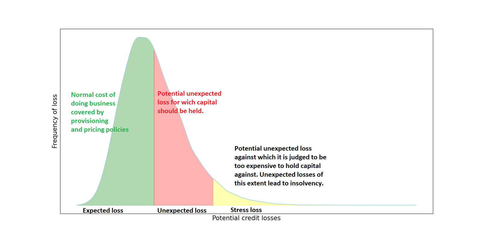
Figure 1: Loss distribution. Source: Page 8 in [39].

In the following sections, we write the expression of the portfolio EL and UL as functions of the parameters and of the processes introduced above, and introduce the entity’s probability of default.

3.2 Expected loss

The following proposition computes the default probability of each firm and the portfolio EL.

Proposition 3.7.

Let $(\Upsilon_{u})_{u\in\mathbb{N}}$ and $(\mathfrak{R}^{n}_{u}(\mathfrak{d}))_{u\in\mathbb{N}}$ (with $n\in\{1,\ldots,N\}$) be as in A and (2.8). For $(a,\theta)\in\mathbb{R}^{I}\times\mathbb{R}^{I}$, $t\in\mathbb{N}$, $T\in\mathbb{N}^{*}$, and $n\in\{1,\ldots,N\}$, define

$$\mathfrak{L}^{n}(\mathfrak{d},t,T,a,\theta):=\Phi\left(\frac{\log(B^{n})-\mathcal{K}^{n}(\mathfrak{d},t,T,a,\theta)}{\sqrt{\mathcal{L}^{n}(t,T)}}\right),$$

where $\mathcal{K}^{n}(\mathfrak{d},t,T,a,\theta)$ and $\mathcal{L}^{n}(t,T)$ are defined in Remark 2.9. Then, the (conditional) probability of default of the entity $n$ at time $t$ over the horizon $T$ is

$$\mathrm{PD}^{n}_{t,T,\mathfrak{d}}:=\mathbb{P}\left(\mathcal{V}^{n}_{t+T}\leq\mathfrak{B}^{n}|\mathcal{G}_{t}\right)=\mathfrak{L}^{n}(\mathfrak{d},t,T,\mathcal{A}_{t}^{\circ},\Theta_{t}),$$ (3.6)

and the (conditional) EL of the portfolio at time $t$ over the horizon $T$ reads

$$\mathrm{EL}^{N,T}_{t,\mathfrak{d}}:=\mathrm{EL}^{N,T}_{t}=\sum_{n=1}^{N}\mathrm{EAD}_{t+T}^{n}\cdot\mathrm{LGD}_{t+T}^{n}\cdot\mathfrak{L}^{n}(\mathfrak{d},t,T,\mathcal{A}_{t}^{\circ},\Theta_{t}).$$ (3.7)

Proof.

Let $t\in\mathbb{N}$ and $T\in\mathbb{N}^{*}$, for $1\leq n\leq N$, (2.9) gives the law of $\log(\mathcal{V}^{n}_{t+T})|\mathcal{G}_{t}$, we directly obtain (3.6). Moreover,

$$\begin{split}\mathrm{EL}^{N,T}_{t,\mathfrak{d}}&=\mathbb{E}\left[\mathrm{L}^{\mathbb{G},N}_{t+T}|\mathcal{G}_{t}\right]\\ &=\mathbb{E}\left[\sum_{n=1}^{N}\mathrm{EAD}_{t+T}^{n}\cdot\mathrm{LGD}_{t+T}^{n}\cdot\Phi\left(\frac{\log(\mathfrak{B}^{n})-\log(F_{0}^{n})-\mathfrak{m}^{n}(\mathfrak{d},t+T,\mathcal{A}^{\circ}_{t+T})}{\sigma_{\mathfrak{b}^{n}}\sqrt{t+T}}\right)\middle|\mathcal{G}_{t}\right]\\ &=\sum_{n=1}^{N}\mathrm{EAD}_{t+T}^{n}\cdot\mathrm{LGD}_{t+T}^{n}\cdot\mathbb{E}\left[\Phi\left(\frac{\log(B^{n})-\mathfrak{m}^{n}(\mathfrak{d},t+T,\mathcal{A}^{\circ}_{t+T})}{\sigma_{\mathfrak{b}^{n}}\sqrt{t+T}}\right)\middle|\mathcal{G}_{t}\right],\end{split}$$

where the last equality comes from Assumption 3.1(1)-(3). However,

$$\mathfrak{m}^{n}(\mathfrak{d},t+T,\mathcal{A}^{\circ}_{t+T}) =\mathfrak{a}^{n\cdot}\left(\mathcal{A}^{\circ}_{t+T}-v(\mathfrak{d}_{0})\right)+\log(\mathfrak{R}^{n}_{t+T}(\mathfrak{d}))$$

$$=\mathfrak{a}^{n\cdot}\left(\mathcal{A}^{\circ}_{t}+\sum_{u=t+1}^{t+T}\Theta_{u}-v(\mathfrak{d}_{0})\right)+\log(\mathfrak{R}^{n}_{t+T}(\mathfrak{d}))$$

$$=\mathfrak{m}^{n}(\mathfrak{d},t,\mathcal{A}^{\circ}_{t})+\log(\mathfrak{R}^{n}_{t+T}(\mathfrak{d}))-\log(\mathfrak{R}^{n}_{t}(\mathfrak{d}))+\mathfrak{a}^{n\cdot}\sum_{u=1}^{T}\Theta_{t+u}.$$

For all $\theta\in\mathbb{R}^{d}$, according to (A.3),

$$\left(\sum_{u=1}^{T}\Theta_{t+u}\middle|\Theta_{t}=\theta\right)\sim\mathcal{N}\left(\Gamma\Upsilon_{T-1}\theta+\left(\sum_{u=1}^{T}\Upsilon_{u-1}\right)\mu,\varepsilon^{2}\sum_{u=1}^{T}\Upsilon_{T-u}\Sigma(\Upsilon_{T-u})^{\top}\right),$$

Let $n\in\{1,\ldots,N\}$, therefore,

$$\left(\mathfrak{a}^{n\cdot}\sum_{u=1}^{T}\Theta_{t+u}\middle|\mathcal{G}_{t}\right)\sim\mathcal{N}\left(\mathfrak{a}^{n\cdot}\Gamma\Upsilon_{T-1}\Theta_{t}+\mathfrak{a}^{n\cdot}\left(\sum_{u=1}^{T}\Upsilon_{u-1}\right)\mu,\varepsilon^{2}\sum_{u=1}^{T}(\mathfrak{a}^{n\cdot}\Upsilon_{T-u})\Sigma(\mathfrak{a}^{n\cdot}\Upsilon_{T-u})^{\top}\right).$$

Then

$$\left(\frac{\log(B^{n})-\mathfrak{m}^{n}(\mathfrak{d},t+T,\mathcal{A}^{\circ}_{t+T})}{\sigma_{\mathfrak{b}^{n}}\sqrt{t+T}}\middle|\mathcal{G}_{t}\right)\sim\frac{\mathcal{S}^{n}(T)}{\sigma_{\mathfrak{b}^{n}}\sqrt{t+T}}\mathcal{X}^{n}+\frac{\log(B^{n})-\mathcal{K}^{n}(\mathfrak{d},t,T,\mathcal{A}^{\circ}_{t},\Theta_{t})}{\sigma_{\mathfrak{b}^{n}}\sqrt{t+T}},$$ (3.8)

where $(\mathcal{X}^{n})_{1\leq n\leq N}\sim\mathcal{N}(\mathbf{0},\mathbf{I}_{N})$, and where $\mathcal{K}^{n}(\mathfrak{d},t,T,\mathcal{A}^{\circ}_{t},\Theta_{t})$ is defined in (2.13) and where

$$\mathcal{S}^{n}(T):=\varepsilon\sqrt{\sum_{u=1}^{T}(\mathfrak{a}^{n\cdot}\Upsilon_{T-u})\Sigma(\mathfrak{a}^{n\cdot}\Upsilon_{T-u})^{\top}}.$$

We then have

$$\begin{split}&\mathbb{E}\left[\Phi\left(\frac{\mathcal{S}^{n}(T)}{\sigma_{\mathfrak{b}^{n}}\sqrt{t+T}}\mathcal{X}^{n}+\frac{\log(B^{n})-\mathcal{K}^{n}(\mathfrak{d},t,T,\mathcal{A}^{\circ}_{t},\Theta_{t})}{\sigma_{\mathfrak{b}^{n}}\sqrt{t+T}}\right)\middle|\mathcal{G}_{t}\right]\\ &\qquad\qquad=\mathbb{E}_{\mathcal{X}^{n}}\left[\Phi\left(\frac{\mathcal{S}^{n}(T)}{\sigma_{\mathfrak{b}^{n}}\sqrt{t+T}}\mathcal{X}^{n}+\frac{\log(B^{n})-\mathcal{K}^{n}(\mathfrak{d},t,T,\mathcal{A}^{\circ}_{t},\Theta_{t})}{\sigma_{\mathfrak{b}^{n}}\sqrt{t+T}}\right)\right]\\ &\qquad\qquad=\int_{-\infty}^{+\infty}\Phi\left(\frac{\mathcal{S}^{n}(T)}{\sigma_{\mathfrak{b}^{n}}\sqrt{(t+T)}}x+\frac{\log(B^{n})-\mathcal{K}^{n}(\mathfrak{d},t,T,\mathcal{A}^{\circ}_{t},\Theta_{t})}{\sigma_{\mathfrak{b}^{n}}\sqrt{(t+T)}}\right)\phi(x)dx\\ &\qquad\qquad=\Phi\left(\frac{\log(B^{n})-\mathcal{K}^{n}(\mathfrak{d},t,T,\mathcal{A}^{\circ}_{t},\Theta_{t})}{\sqrt{\mathcal{L}^{n}(t,T)}}\right),\end{split}$$

where $\mathcal{L}^{n}(t,T)$ is defined in (2.14), and the conclusion follows.

The last equality comes from the following result found in [37, Page 1063]: if $\Phi$ and $\phi$ are the Gaussian cumulative distribution and density functions, then for $a,b\in\mathbb{R}$,

$$\int_{-\infty}^{+\infty}\Phi(a+bx)\phi(x)dx=\Phi\left(\frac{a}{\sqrt{1+b^{2}}}\right).$$ (3.9)

∎

3.3 Unexpected loss

At time $t\in\mathbb{N}$, it follows from the definition of $\mathrm{UL}$ in (3.4) that we need to compute the quantile of the (proxy of the) loss distribution $L^{\mathbb{G},N}_{t}$. For $\alpha\in(0,1)$, we obtain from Theorem 3.5,

$$\begin{split}1-\alpha&=\mathbb{P}\left[L_{t+T}^{\mathbb{G},N}\leq\mathrm{VaR}^{\alpha,N,T}_{t}\middle|\mathcal{G}_{t}\right]\\ &=\mathbb{P}\left[\sum_{n=1}^{N}\mathrm{EAD}_{t+T}^{n}\cdot\mathrm{LGD}_{t+T}^{n}\cdot\Phi\left(\frac{\log(B^{n})-\mathfrak{m}^{n}(\mathfrak{d},t+T,\mathcal{A}^{\circ}_{t+T})}{\sigma_{\mathfrak{b}^{n}}\sqrt{t+T}}\right)\leq\mathrm{VaR}^{\alpha,N,T}_{t}\middle|\mathcal{G}_{t}\right].\end{split}$$ (3.10)

However, it follows from (3.8),

$$\begin{split}1-\alpha=\mathbb{P}_{\mathcal{X}^{1},\ldots,\mathcal{X}^{N}}\left[\sum_{n=1}^{N}\mathrm{EAD}_{t+T}^{n}\cdot\mathrm{LGD}_{t+T}^{n}\cdot\Phi\left(\frac{\mathcal{S}^{n}(T)}{\sigma_{\mathfrak{b}^{n}}\sqrt{t+T}}\mathcal{X}^{n}+\frac{\log(B^{n})-\mathcal{K}^{n}(\mathfrak{d},t,T,\mathcal{A}^{\circ}_{t},\Theta_{t})}{\sigma_{\mathfrak{b}^{n}}\sqrt{t+T}}\right)\leq\mathrm{VaR}^{\alpha,N,T}_{t}\right].\end{split}$$ (3.11)

Since the quantile function is not linear, one cannot find an analytical solution. Therefore, a numerical solution is needed. Recall that we must simulate $(\mathcal{X}^{1},\ldots,\mathcal{X}^{N})$ to find $\mathrm{VaR}^{\alpha,N,T}_{t}$, which will also be a function of the random variables $(\mathcal{A}^{\circ}_{t},\Theta_{t})$, of dimension $2I$. This can be solved for example by Monte Carlo [22] or by deep learning techniques [5].

3.4 Projection of one-year risk measures

At this stage, we use (3.6) to compute, for each $n\in\{1,\ldots,N\}$, the probability of default of a given firm $n$ at maturity $T$, stressed by (deterministic) carbon taxes $\mathfrak{d}$. We can also calculate EL according to (3.7) and UL from (3.11). We just need the parameters, especially $\mathbf{a}^{n}$, $\sigma_{\mathfrak{b}^{n}}^{2}$, $F_{0}^{n}$, and $\mathfrak{B}^{n}$. We can distinguish two ways to determine them:

1. Firm’s view: $\mathbf{a}^{n}$, $\sigma_{\mathfrak{b}^{n}}^{2}$ and $F_{0}^{n}$ are calibrated on the firm’s historical free cash flows, while $\mathfrak{B}^{n}$ relates to the principal of its loans.

2. Portfolio’s view: if we assume that there is just one risk class in the portfolio so that all the firms have the same $\mathbf{a}^{n}$, $\sigma_{\mathfrak{b}^{n}}^{2}$, and $B^{n}$ (and not $\mathfrak{B}^{n}$), then knowing the historical default of the portfolio, we can use a log-likelihood maximization as in Gordy and Heitfield [21] to determine them.

Let us introduce the following assumption related to the portfolio view.

Assumption 3.8.

There is only one risk class in the given portfolio, namely for any $1\leq n\leq N$, $\mathbf{a}^{n}=\mathbf{a}^{1}$, $\sigma_{\mathfrak{b}^{n}}^{2}=\sigma_{\mathfrak{b}^{1}}^{2}$, and $B^{n}=B^{1}$.

In practice, banks need to compute the one-year probability of default. We thus simplify the risk measures introduced previously by taking from now $T=1$.

Corollary 3.9.

Under Assumption 3.8, for $t\in\mathbb{N}$ and $1\leq n\leq N$, the one-year (conditional) probability of default of firm $n$ at time $t$ is

$$\mathrm{PD}^{n}_{t,1,\mathfrak{d}}=\Phi\left(\frac{\log(B^{1})-\mathcal{K}^{1}(\mathfrak{d},t,1,\mathcal{A}_{t}^{\circ},\Theta_{t})}{\sqrt{\mathcal{L}^{1}(t,1)}}\right).$$ (3.12)

Proof.

Let $t\in\mathbb{N}$ and $1\leq n\leq N$,

$$\begin{split}\mathcal{K}^{n}(\mathfrak{d},t,1,\mathcal{A}^{\circ}_{t},\Theta_{t})&=\mathfrak{m}^{n}(\mathfrak{d},t,\mathcal{A}^{\circ}_{t})+\log(\mathfrak{R}^{1}_{t+1}(\mathfrak{d}))-\log(\mathfrak{R}^{1}_{t}(\mathfrak{d}))+\mathfrak{a}^{1\cdot}\Gamma\Upsilon_{0}\Theta_{t}+\mathfrak{a}^{1\cdot}\Upsilon_{0}\mu\\ &=\mathfrak{m}^{1}(\mathfrak{d},t,\mathcal{A}^{\circ}_{t})+\log(\mathfrak{R}^{1}_{t+1}(\mathfrak{d}))-\log(\mathfrak{R}^{1}_{t}(\mathfrak{d}))+\mathfrak{a}^{1\cdot}\Gamma\Theta_{t}+\mathfrak{a}^{1\cdot}\mu\\ &=\mathcal{K}^{1}(\mathfrak{d},t,1,\mathcal{A}^{\circ}_{t},\Theta_{t}),\end{split}$$

given that $\Upsilon_{0}=\mathbf{I}_{I}$ and from Assumption 3.8. We also have

$$\mathcal{L}^{n}(t,1)={\sigma_{\mathfrak{b}^{1}}^{2}(t+1)+(\mathfrak{a}^{1\cdot}\Upsilon_{0})\Sigma(\mathfrak{a}^{1\cdot}\Upsilon_{0})^{\top}}={\sigma_{\mathfrak{b}^{1}}^{2}(t+1)+(\mathfrak{a}^{1\cdot})\Sigma(\mathfrak{a}^{1\cdot})^{\top}}=\mathcal{L}^{1}(t,1).$$

∎

3.4.1 Expected loss

The following corollary, whose proof follows from Corollary 3.9, gives a simplified formula for EL.

Proposition 3.10.

Under Assumption 3.8, the one-year (conditional) EL of the portfolio at time $t$ is (with $\mathrm{PD}^{1}_{t,1,\mathfrak{d}}$ defined in Corollary 3.9)

$$\mathrm{EL}^{N,T}_{t,\mathfrak{d}}=\left(\sum_{n=1}^{N}\mathrm{EAD}_{t+1}^{n}\cdot\mathrm{LGD}_{t+1}^{n}\right)\cdot\mathrm{PD}^{1}_{t,1,\mathfrak{d}}.$$ (3.13)

3.4.2 Unexpected loss

We saw in (3.11) that determining the UL is not possible analytically and is numerically intensive (since quantiles depend on rare events and because of the dimension of the macroeconomic factors). However, Assumption 3.4 allows us to further simplify the formula for UL.

Corollary 3.11.

Under Assumption 3.8, the one-year (conditional) UL of the portfolio at time $t$ is

$$\mathrm{UL}^{N,T}_{t,\mathfrak{d},\alpha}=\left(\sum_{n=1}^{N}\mathrm{EAD}_{t+T}^{n}\cdot\mathrm{LGD}_{t+T}^{n}\right)\left[\Phi\left(\frac{\mathcal{S}^{1}(t,T)\Phi^{-1}(1-\alpha)+\log(B^{1})-\mathcal{K}^{1}(\mathfrak{d},t,T,\mathcal{A}^{\circ}_{t},\Theta_{t})}{\sigma_{\mathfrak{b}^{1}}\sqrt{t+T}}\right)-\mathrm{PD}^{1}_{t,1,\mathfrak{d}}\right].$$ (3.14)

Proof.

From (3.11), we have

$$\begin{split}1-\alpha&=\mathbb{P}_{\mathcal{X}^{1},\ldots,\mathcal{X}^{N}}\left[\sum_{n=1}^{N}\mathrm{EAD}_{t+T}^{n}\cdot\mathrm{LGD}_{t+T}^{n}\cdot\Phi\left(\frac{\mathcal{S}^{n}(T)\mathcal{X}^{n}+\log(B^{n})-\mathcal{K}^{n}(\mathfrak{d},t,T,\mathcal{A}^{\circ}_{t},\Theta_{t})}{\sigma_{\mathfrak{b}^{n}}\sqrt{t+T}}\right)\leq\mathrm{VaR}^{\alpha,N,T}_{t}\right],\end{split}$$

but with Corollary 3.9,

$$\begin{split}1-\alpha&=\mathbb{P}_{\mathcal{X}^{1}}\left[\Phi\left(\frac{\mathcal{S}^{1}(t,T)\mathcal{X}^{1}+\log(B^{1})-\mathcal{K}^{1}(\mathfrak{d},t,T,\mathcal{A}^{\circ}_{t},\Theta_{t})}{\sigma_{\mathfrak{b}^{1}}\sqrt{t+T}}\right)\leq\frac{\mathrm{VaR}^{\alpha,N,T}_{t}}{\sum_{n=1}^{N}\mathrm{EAD}_{t+T}^{n}\cdot\mathrm{LGD}_{t+T}^{n}}\right]\\ &=\mathbb{P}_{\mathcal{X}^{1}}\left[\frac{\mathcal{S}^{1}(t,T)\mathcal{X}^{1}+\log(B^{1})-\mathcal{K}^{1}(\mathfrak{d},t,T,\mathcal{A}^{\circ}_{t},\Theta_{t})}{\sigma_{\mathfrak{b}^{1}}\sqrt{t+T}}\leq\Phi^{-1}\left(\frac{\mathrm{VaR}^{\alpha,N,T}_{t}}{\sum_{n=1}^{N}\mathrm{EAD}_{t+T}^{n}\cdot\mathrm{LGD}_{t+T}^{n}}\right)\right]\\ &=\mathbb{P}_{\mathcal{X}^{1}}\left[\mathcal{X}^{1}\leq\frac{1}{\mathcal{S}^{1}(t,T)}\left(\sigma_{\mathfrak{b}^{1}}\sqrt{t+T}\Phi^{-1}\left(\frac{\mathrm{VaR}^{\alpha,N,T}_{t}}{\sum_{n=1}^{N}\mathrm{EAD}_{t+T}^{n}\cdot\mathrm{LGD}_{t+T}^{n}}\right)-\log(B^{1})+\mathcal{K}^{1}(\mathfrak{d},t,T,\mathcal{A}^{\circ}_{t},\Theta_{t})\right)\right].\end{split}$$

Then the corollary follows from

$$\mathrm{VaR}^{\alpha,N,T}_{t}=\left(\sum_{n=1}^{N}\mathrm{EAD}_{t+T}^{n}\cdot\mathrm{LGD}_{t+T}^{n}\right)\cdot\Phi\left(\frac{\mathcal{S}^{1}(t,T)\Phi^{-1}(1-\alpha)+\log(B^{1})-\mathcal{K}^{1}(\mathfrak{d},t,T,\mathcal{A}^{\circ}_{t},\Theta_{t})}{\sigma_{\mathfrak{b}^{1}}\sqrt{t+T}}\right).$$

∎

3.5 Sensitivity of losses to carbon price

We would like to quantify the variation of losses for a given variation in the carbon price.

Definition 3.12.

For our portfolio of $N$ firms and for $\alpha\in(0,1)$, we introduce the sensitivity of expected and unexpected losses to carbon taxes, at time $t\in\mathbb{N}$ over the horizon $T\in\mathbb{N}^{*}$, and for a given sequence of carbon taxes $\mathfrak{d}$, respectively denoted $\Gamma^{N,T,\mathrm{EL}}_{t,\mathfrak{d}}(\mathfrak{U})$ and $\Gamma^{N,T,\mathrm{UL}}_{t,\mathfrak{d},\alpha}(\mathfrak{U})$, as being,

$$\Gamma^{N,T,\mathrm{EL}}_{t,\mathfrak{d}}(\mathfrak{U}):=\lim_{\vartheta\to 0}\frac{\mathrm{EL}^{N,T}_{t,\mathfrak{d}+\vartheta\mathfrak{U}}-\mathrm{EL}^{N,T}_{t,\mathfrak{d}}}{\vartheta}\qquad\textrm{and}\qquad\Gamma^{N,T,\mathrm{UL}}_{t,\mathfrak{d},\alpha}(\mathfrak{U}):=\lim_{\vartheta\to 0}\frac{\mathrm{UL}^{N,T}_{t,\mathfrak{d}+\vartheta\mathfrak{U},\alpha}-\mathrm{UL}^{N,T}_{t,\mathfrak{d},\alpha}}{\vartheta},$$ (3.15)

where $\mathfrak{U}\in([0,1)^{I}\times[0,1)^{I\times I}\times[0,1)^{I})^{\mathbb{N}}$ is chosen so that there exists a neighbourhood $v$ of the origin so that for all $\vartheta\in v$, $\mathfrak{d}+\vartheta\mathfrak{U}\in([0,1)^{I}\times[0,1)^{I\times I}\times[0,1)^{I})^{\mathbb{N}}$.

These sensitivities can be computed and understood in different ways depending of the direction $\mathfrak{U}$: either in relation to the entire tax trajectory, or in relation to all taxes at a given date, or in relation to one of the three taxes, or in relation to a sector, and so on. We could also (and will so in a future note) give the results for stochastic carbon price in the transition period. In this case, if the productivity $\Theta$ and the carbon price $\delta$ are independent, it is enough to add in the previous results, the expectation conditionally to $\delta$.

4 Estimation and calibration

Assume that the time unit is year. We will calibrate the model parameters on a set of data ranging from year $\mathfrak{t}_{0}$ to $\mathfrak{t}_{1}$. In practice, $\mathfrak{t}_{0}=1978$ and $\mathfrak{t}_{1}=t_{\circ}=2021$. For each sector $i\in\mathcal{I}$ and $0\leq t<t_{\circ}$, we observe the output $Y_{t}^{i}$, the labor $N_{t}^{i}$, the intermediary input $(Z_{t}^{ji})_{j\in\mathcal{I}}$, and the consumption $C_{t}^{i}$ (recall that the transition starts at year $t_{\circ}$ so $[0,t_{\circ})$ is the past). For the sake of clarity, we will omit the dependence of each estimated parameter on $t_{\circ}$.

4.1 Calibration of carbon taxes

We assume here that the carbon price is deterministic. The regulator fixes the transition time horizon $t_{\star}\in\mathbb{N}^{*}$, the carbon price at the beginning of the transition $P_{carbon}>0$, at the end of the transition $\delta_{t_{\star}}>P_{carbon}$, and the annual evolution rate $\eta_{\delta}>0$. Then, for all $t\in\mathbb{N}$,

$$\delta_{t}=\left\{\begin{array}[]{ll}\displaystyle P_{carbon},&\mbox{if }t<t_{\circ},\\ \displaystyle P_{carbon}(1+\eta_{\delta})^{t-t_{\circ}},&\mbox{if }t\in\{t_{\circ},\ldots,t_{\star}\},\\ \displaystyle P_{carbon}=\delta_{t_{\circ}}(1+\eta_{\delta})^{t_{\star}-t_{\circ}},&\mbox{otherwise}.\end{array}\right.$$ (4.1)

We denote for any sector $i\in\mathcal{I}$,

• $t=t_{\circ}$ the first year of the transition;

• $Y_{t_{\circ}}^{i}$ the output at time $t_{\circ}$;

• $P_{t_{\circ}}^{i}$ the aggregate price at time $t_{\circ}$;

• $C_{t_{\circ}}^{i}$ the sectoral consumption (or value added) of households at time $t_{\circ}$.

The taxes are calibrated on realized emissions [14], based on Devulder and Lisack [12], to the chosen year $t_{\circ}$, then for all $i\in\mathcal{I}$:

• the tax rate on firms production is set such that

  $$\tau_{t_{\circ}}^{i}Y_{t_{\circ}}^{i}P_{t_{\circ}}^{i}=P_{carbon}E_{t_{\circ}}^{i,F},$$

  where $E_{t_{\circ}}^{i,F}$ are the GHG emissions (in tonnes of CO2-equivalent) by all the firms of the sector $i$ at $t_{\circ}$. Then for all $t\in\{t_{\circ},\ldots,t_{\star}\}$, we have

  $$\tau_{t}^{i}(\delta_{t}):=\delta_{t}\frac{E_{t_{\circ}}^{i,F}}{Y_{t_{\circ}}^{i}P_{t_{\circ}}^{i}},$$ (4.2)

• the tax rate on households final consumption is set such that

  $$\kappa_{t_{\circ}}^{i}P_{t_{\circ}}^{i}C_{t_{\circ}}^{i}:=P_{carbon}E_{i,t_{\circ}}^{i,H},$$

  where $E_{t_{\circ}}^{i,H}$ is the GHG emitted (in tonnes of CO2-equivalent) by households through their consumption in sector $i$. Then for all $t\in\{t_{\circ},\ldots,t_{\star}\}$, we have

  $$\kappa_{t}^{i}(\delta_{t}):=\delta_{t}\frac{E_{i,t_{\circ}}^{i,H}}{P_{t_{\circ}}^{i}C_{t_{\circ}}^{i}}.$$ (4.3)

• the tax rate on firms intermediate consumption, for each sector $i$ and $j$, is set such that

  $$\sum_{j=1}^{I}\zeta_{t_{\circ}}^{ji}P_{t_{\circ}}^{j}Z_{t_{\circ}}^{ji}:=P_{carbon}E_{t_{\circ}}^{i,F}.$$ (4.4)

  Then for all $t\in\{t_{\circ},\ldots,t_{\star}\}$, we have

  $$\zeta_{t}^{ji}(\delta_{t})=\delta_{t}\frac{E_{t_{\circ}}^{i,F}}{I\times P_{t_{\circ}}^{j}Z_{t_{\circ}}^{ji}}.$$ (4.5)

The values $\frac{E_{t_{\circ}}^{i,F}}{Y_{t_{\circ}}^{i}P_{t_{\circ}}^{i}}$, $\frac{E_{i,t_{\circ}}^{i,CO2,H}}{P_{t_{\circ}}^{i}C_{t_{\circ}}^{i}}$ and $\frac{E_{t_{\circ}}^{i,F}}{I\times P_{t_{\circ}}^{j}Z_{t_{\circ}}^{ji}}$ represent the carbon intensities of sector $i$ production, consumption and intermediary input respectively, which we assume fixed over the transition. This is a very strong assumption here, because we can think that the greening of the economy will lead to a decrease in carbon intensity. Moreover, we assume that taxes increase. However, there are several scenarios that could be considered, including taxes that would increase until a certain year before leveling off or even decreasing. The tax on production would increase when the tax on households would stabilize or disappear (in order to avoid social movements) and so on. The framework can be adapted to various sectors, scenarios, and tax evolutions.

4.2 Calibration of economic parameters

As in [16], we assume a unitary Frisch elasticity of labor supply so $\varphi=1$ and the utility of consumption is logarithmic so $\sigma=1$. Similarly, for any $i,j\in\mathcal{I}$, the input shares, $\boldsymbol{\lambda}^{ij}$ , are estimated as dollar payments from sector $j$ to sector $i$ expressed as a fraction of the value of production in sector $j$. The parameter $\psi^{i}$ is then obtained by

$$\psi^{i}=1-\sum_{j\in\mathcal{I}}\boldsymbol{\lambda}^{ji},$$

and we get $(\widehat{\boldsymbol{\lambda}}^{ij})_{i,j\in\mathcal{I}}$ and $(\widehat{\psi}^{i})_{i\in\mathcal{I}}$. We can then compute the functions $\Psi$ in (1.18) and $\Lambda$ in (1.19). We can also compute the sectoral consumption growth $\left(\Delta^{{C}}_{t}=(\log(C_{t}^{i})-\log(C_{t-1}^{i}))_{j\in\mathcal{I}}\right)_{t\in\mathfrak{t}_{0},\dots,\mathfrak{t}_{1}-1}$ directly from data.

Without carbon tax in any sector, it follows from (1.35) in Corollary 1.14 that, for each $t\in\{\mathfrak{t}_{0},\dots,\mathfrak{t}_{1}-1\}$, the computed consumption growth $\Delta^{{C}}_{t}$ is equal to $\Delta^{{C}}_{t}=(\mathbf{I}_{I}-\widehat{\boldsymbol{\lambda}})^{-1}\widehat{\Theta}_{t}$ when $\mathbf{I}_{I}-\widehat{\boldsymbol{\lambda}}$ is not singular; hence $\widehat{\Theta}_{t}=(\mathbf{I}_{I}-\widehat{\boldsymbol{\lambda}})\Delta^{{C}}_{t}$ and we can easily compute the estimations $\widehat{\mu}$, $\widehat{\Gamma}$, and $\widehat{\Sigma}$, and then $\widehat{\overline{\mu}}$ and $\widehat{\overline{\Sigma}}$ of the VAR(1) parameters $\mu$, $\Gamma$, $\Sigma$, $\overline{\mu}$, and $\overline{\Sigma}$ (all defined in Standing Assumption 1.1).

4.3 Calibration of firm and of the credit model parameters

Recall that we have a portfolio with $N\in\mathbb{N}^{*}$ firms (or credit) at time $t_{\circ}$. For each firm $n\in\{1,\ldots,N\}$, we have its historical cash flows $(F_{t}^{n})_{t\in\mathfrak{t}_{0},\dots,\mathfrak{t}_{1}-1}$, hence its log-cash flow growths. We assume that we can divide our portfolio in $M\leq N$ disjunct groups $g_{1},\ldots,g_{M}$ so that each group represents a single risk class. For any $t\in\{\mathfrak{t}_{0},\dots,\mathfrak{t}_{1}-1\}$ and $1\leq m\leq M$, we denote by $r_{t}^{m}$ (resp. $d_{t}^{m}$) the number of firms in $g_{m}$ rated at the beginning of the year $t$ (resp. defaulted during the year $t$). In particular, $r_{\mathfrak{t}_{0}}=\#g_{m}$. Within each group $g_{m}$, all the firms behave in the same way as there is only one risk class. We fix $m_{\star}:=\min{\{n\in\{1,\ldots,N\}\text{ such that }n\in g_{m}\}}$ and, for each $n\in g_{m}$, $\mathbf{a}^{n}=\mathbf{a}^{m_{\star}}$, $\sigma_{\mathfrak{b}^{n}}=\sigma_{\mathfrak{b}^{m_{\star}}}$, and $B^{n}=B^{m_{\star}}$. We then proceed as follows:

1. Knowing the consumption growth $\left(\Delta^{{C}}_{t}\right)_{t\in\{\mathfrak{t}_{0},\dots,\mathfrak{t}_{1}-1\}}$, we calibrate the factor loading $\widehat{\mathbf{a}}_{m_{\star}}$ and the standard deviation $\widehat{\sigma}_{m_{\star}}$, according to Assumptions 2.1 and 2.4, appealing to the regression

   $$\sum_{n\in g_{m}}\omega_{t}^{n}=(\#g_{m})\mathbf{a}^{m_{\star}}\Delta^{{C}}_{t}+\sqrt{\#g_{m}}\sigma_{\mathfrak{b}^{m_{\star}}}\mathfrak{u}_{t}\quad\text{where}\quad\mathfrak{u}_{t}\sim\mathcal{N}(0,1),\quad\text{for all}\quad t\in\{\mathfrak{t}_{0},\dots,\mathfrak{t}_{1}-1\}.$$ (4.6)

2. We then estimate the barrier $B^{m_{\star}}$ by MLE as detailed in Gordy and Heitfield in [21, Section 3]:

   we compute

   $$\widehat{B}^{m_{\star}}:=\operatorname*{arg\,max}_{B^{m_{\star}}\in\mathbb{R}^{+}}\mathcal{L}(B^{m_{\star}}),$$

   where $\mathcal{L}(B^{m_{\star}})$ is the log-likelihood function defined by

   $$\mathcal{L}(B^{m_{\star}}):=\sum_{t=\mathfrak{t}_{0}}^{\mathfrak{t}_{1}-1}\log\left(\int_{\mathbb{R}^{2I}}\mathbb{P}[D^{m_{\star}}=d_{t}^{m}|(a,\theta)]d\mathbb{P}[(\mathcal{A}_{t}^{\circ},\Theta_{t})\leq(a,\theta)]\right),$$

   and where

   $$\mathbb{P}[D^{m_{\star}}=d_{t}^{m}|(\mathcal{A}_{t}^{\circ},\Theta_{t})]={\binom{r_{t}^{m}}{d_{t}^{m}}}(\mathrm{PD}^{m_{\star}}_{t,1,0})^{d_{t}^{m}}\Big{(}1-\mathrm{PD}^{m_{\star}}_{t,1,0}\Big{)}^{r_{t}^{m}-d_{t}^{m}},$$

   with $D^{m_{\star}}$ the Binomial random variable standing for the conditional number of defaults, and $\mathrm{PD}^{m_{\star}}_{t,1,0}$ in Corollary 3.9, depending on $\sigma_{\mathfrak{b}^{m_{\star}}}=\widehat{\sigma}_{\mathfrak{b}^{m_{\star}}}$, $\mathbf{a}^{m_{\star}}=\widehat{\mathbf{a}}^{m_{\star}}$, $\mathfrak{d}=0$ and on $B^{m_{\star}}$.

4.4 Expected and Unexpected losses

Suppose that we have chosen or estimated all the economic parameters ($\varphi,\sigma,\psi,\boldsymbol{\lambda},\mu,\Gamma,\Sigma$) and firm specific parameters ($(B^{n},\mathbf{a}^{n},F_{0}^{n},\sigma_{\mathfrak{b}^{n}})_{1\leq n\leq N}$), thanks to the previous equations. We give ourselves a trajectory of carbon price $\delta$, then, for all $t\in\{t_{\circ},\ldots,t_{\star}\}$, PD, EL and UL are computed by Monte Carlo simulations following the formulae below. We simulate $M\in\mathbb{N}^{*}$ paths of $(\Theta_{t_{\circ}}^{p},\ldots,\Theta_{t_{\star}}^{p})$ indexed by $p\in\{1,\ldots,M\}$, as a VAR(1) process, and we derive $((\mathcal{A}_{t_{\circ}}^{\circ})^{p},\ldots,(\mathcal{A}_{t_{\star}}^{\circ})^{p})$. For any $t\in\{t_{\circ},\ldots,t_{\star}\}$:

• for any $n\in\{1,\ldots,N\}$, from (3.12), the estimated one-year probability of default of firm $n$ is

  $$\widehat{\mathrm{PD}}^{n,M}_{t,1,\mathfrak{d}}:=\frac{1}{M}\sum_{p=1}^{M}\Phi\left(\frac{\log(B^{n})-\mathcal{K}^{n}(\mathfrak{d},t,1,(\mathcal{A}_{t}^{\circ})^{p},\Theta^{p}_{t})}{\sqrt{\mathcal{L}^{n}(t,1)}}\right),$$ (4.7)

• the one-year expected loss is, from (3.13),

  $$\widehat{\mathrm{EL}}^{N,T}_{t,\mathfrak{d}}:=\frac{1}{M}\sum_{p=1}^{M}\sum_{n=1}^{N}\mathrm{EAD}_{t+1}^{n}\cdot\mathrm{LGD}_{t+1}^{n}\cdot\widehat{\mathrm{PD}}^{n,M}_{t,1,\mathfrak{d}},$$ (4.8)

• the one-year unexpected loss is, from (3.14),

  $$\small\widehat{\mathrm{UL}}^{N,T}_{t,\mathfrak{d},\alpha}:=q_{\alpha,M}\left(\left\{\sum_{n=1}^{N}\mathrm{EAD}_{t+1}^{n}\cdot\mathrm{LGD}_{t+1}^{n}\cdot\Phi\left(\frac{\log(B^{n})-\mathcal{K}^{n}(\mathfrak{d},t,1,(\mathcal{A}_{t}^{\circ})^{p},\Theta^{p}_{t})}{\sqrt{\mathcal{L}^{n}(t,1)}}\right)\right\}_{1\leq p\leq M}\right)-\widehat{\mathrm{EL}}^{N,T}_{t,\mathfrak{d}},$$ (4.9)

  where $q_{\alpha,M}(\{Y^{1},\ldots,Y^{M}\})$ denotes the empirical $\alpha$-quantile of the distribution of $Y$.

4.5 Summary of the process

More concretely, the goal is to project, for a given portfolio, the $T=1$ year probability of default, as well as the expected and unexpected losses between year $t_{\circ}$ and year $t_{\star}$, given (1) the number of firms rated $r_{t}$ and defaulted $d_{t}$ between $\mathfrak{t}_{0}$ and $\mathfrak{t}_{1}-1$, (2) all the firms’ cash flows $(F_{t}^{n})_{1\leq n\leq N}$ between $\mathfrak{t}_{0}$ and $\mathfrak{t}_{1}-1$,w (3) the macroeconomic variables observed between $\mathfrak{t}_{0}$ and $\mathfrak{t}_{1}-1$, and (4) the carbon price dynamics $(\delta_{t})_{t\in\{t_{\circ},\ldots,t_{\star}\}}$ or carbon taxes dynamics $(\mathfrak{d}_{t})_{t\in\{t_{\circ},\ldots,t_{\star}\}}$ given by the regulator. We proceed as follows:

1. From the macroeconomic historical data, we estimate the productivity parameters $\widehat{\Gamma}$, $\widehat{\mu}$ and $\widehat{\Sigma}$, as well as the elasticities $\widehat{\psi}$ and $\widehat{\boldsymbol{\lambda}}$ as described in Subsection 4.2.

2. For each $n\in\{1,\ldots,N\}$, we estimate the parameters $B^{n}$, $\sigma_{\mathfrak{b}^{n}}$, $\mathbf{a}^{n}$ using Subsections 4.3, yielding $\widehat{B}^{n}$, $\widehat{\sigma}_{\mathfrak{b}^{n}}$, $\widehat{\mathbf{a}}^{n}$.

3. We compute the carbon taxes from the carbon price dynamics $(\mathfrak{d}_{t})_{t_{\circ}\leq t\leq t_{\star}}$ as defined in Subsection 4.1, then the tax function $v$ defined in (1.23).

4. We fix a large enough integer $M$, and simulate $M$ paths of the productivity process $(\Theta_{t}^{p})_{t_{\circ}\leq t\leq t_{\star}}$, then we derive $((\mathcal{A}_{t}^{\circ})^{p})_{t_{\circ}\leq t\leq t_{\star}}$ as defined in Assumption 1.1. For each $n\in\{1,\ldots,N\}$, we compute the one-year probability of default $\widehat{\mathrm{PD}}^{n,M}_{t,1,\mathfrak{d}}$, for each $t_{\circ}\leq t\leq t_{\star}$, using (4.7).

5. We compute the expected (resp. unexpected) losses $\widehat{\mathrm{EL}}^{N,T}_{t,\mathfrak{d}}$ (resp. $\widehat{\mathrm{UL}}^{N,T}_{t,\mathfrak{d},\alpha}$), for each $t_{\circ}\leq t\leq t_{\star}$, using (4.8) (resp. (4.9)).

6. We fix the direction $\mathfrak{U}$ and a small step $\vartheta$, and repeat 3.-4.-5. replacing $\mathfrak{d}$ by $\mathfrak{d}+\vartheta\mathfrak{U}$. Finally, we approach the sensitivity of the losses with respect to the carbon taxes $\mathfrak{d}$ by finite differences, i.e. for each $t_{\circ}\leq t\leq t_{\star}$,

   $$\widehat{\Gamma}^{N,T,\mathrm{EL}}_{t,\mathfrak{d}}(\mathfrak{U}):=\frac{1}{\vartheta}\left(\widehat{\mathrm{EL}}^{N,T}_{t,\mathfrak{d}+\vartheta\mathfrak{U}}-\widehat{\mathrm{EL}}^{N,T}_{t,\mathfrak{d}}\right)\quad\textrm{and}\quad\widehat{\Gamma}^{N,T,\mathrm{UL}}_{t,\mathfrak{d},\alpha}(\mathfrak{U}):=\frac{1}{\vartheta}\left(\widehat{\mathrm{UL}}^{N,T}_{t,\mathfrak{d}+\vartheta\mathfrak{U},\alpha}-\widehat{\mathrm{UL}}^{N,T}_{t,\mathfrak{d},\alpha}\right).$$ (4.10)

   In the sequel, we choose the direction $\mathfrak{U}\in([0,1)^{I}\times[0,1)^{I\times I}\times[0,1)^{I})^{t_{\star}+1}$ which is equal to $1$ at $t$ and $0$ everywhere else, for each time $t$, and a step $\vartheta=1\%$.

5 Results

5.1 Data

We work on data related to the French economy:

1. Annual consumption, labor, output (displayed on Figure 10 and Figure 11), and intermediary inputs come from Eurostat from 1978 to 2019 (check [4] for details) and are expressed in billion Euros. We also assume that 2020’s data are the same as 2019’s ones in order not to account for the impact of the COVID-19 crisis on data. We thus consider that $t_{\circ}=2021$.

2. The 21 Eurostat sectors are grouped in four categories, Very High Emitting, Very Low Emitting, Low Emitting, High Emitting, based on their carbon intensities (D).

3. The taxes are calibrated on the realized emissions [14] (expressed in tonnes of CO2-equivalent) of the chosen starting year (2021).

4. To perform LASSO regression (C) questioning the relationship between credit risk and economics conditions (as we assumed in Section 3), we use S&P ratings for data on the ratings and default, on a yearly basis from 1995 to 2019, of 7046 large US companies belonging to 13 sectors. We can analyze and use them to compute the historical probability of default (displayed Figure 12) and the migration matrix by sector. The USA macroeconomic time series can be found in the World Bank database and in the FRED Saint-Louis database [15].

5.2 Calibration of economics parameters

For the parameters $\sigma$ and $\varphi$, we use the same values as in Gali [16]: a unitary log-utility $\sigma=1$ and a unitary Frisch elasticity of labor supply $\varphi=1$. We have the parameters of the multisectoral model $(\widehat{\psi}_{i})_{i\in\mathcal{I}}$ and $(\widehat{\boldsymbol{\lambda}}_{ji})_{i,j\in\mathcal{I}}$ in Table 1 and in Table 2.

Emissions Level	Very High	High	Low	Very Low
Elasticity of labor supply	0.083	0.163	0.234	0.374

Table 1: Elasticity of labor supply $\widehat{\psi}$

Emissions Level	Very High	High	Low	Very Low
Very High	0.243	0.010	0.241	0.037
High	0.001	0.302	0.212	0.098
Low	0.053	0.042	0.412	0.107
Very Low	0.004	0.015	0.134	0.220

Table 2: Elasticity of intermediary inputs $\widehat{\boldsymbol{\lambda}}$

We obtain the productivity parameters in Table 3, 4, 5.

Emissions Level	Very High	High	Low	Very Low
$\times 10^{-3}$	5.655	-0.71	0.509	2.901

Table 3: $\widehat{\mu}$

Emissions Level	Very High	High	Low	Very Low
Very High	-0.301	0.077	0.020	0.011
High	0.0820	0.083	-0.001	0.032
Low	-0.218	0.225	0.160	0.292
Very Low	0.552	0.629	0.348	0.674

Table 4: $\widehat{\Gamma}$

Emissions Level	Very High	High	Low	Very Low
Very High	1.199	0.142	0.009	0.055
High	0.142	0.341	0.041	0.035
Low	0.009	0.041	0.040	0.016
Very Low	0.055	0.035	0.016	0.047

Table 5: $\widehat{\Sigma}\times 10^{3}$

In our simulation, we consider four deterministic transition scenarios giving four deterministic carbon price trajectories. The scenarios used come from the NGFS simulations, whose descriptions are given on the NGFS website [31] as follows:

• Net Zero 2050 is an ambitious scenario that limits global warming to $1.5^{\circ}C$ through stringent climate policies and innovation, reaching net zero CO2 emissions around 2050. Some jurisdictions such as the US, EU and Japan reach net zero for all greenhouse gases by this point.

• Divergent Net Zero reaches net-zero by 2050 but with higher costs due to divergent policies introduced across sectors and a quicker phase out of fossil fuels.

• Nationally Determined Contributions (NDCs) includes all pledged policies even if not yet implemented.

• Current Policies assumes that only currently implemented policies are preserved, leading to high physical risks.

We consider a time horizon of ten years with $t_{\circ}=2021$ as starting point, a time step of one year and $t_{\star}=2030$ as ending point. For each scenario, we compute the average annual growth of the tax as displayed in the fourth column of Table 6.

Scenario	2020 Carbon Price (€/ton)	2030 Carbon Price (€/ton)	Average Annual Growth Rate (%)
Current Policies	39.05	39.05	0.
NDCs	39.05	76.46	6.42
Net Zero 2050	39.05	162.67	13.24
Divergent Net Zero	96.43	395.21	10.63

Table 6: Carbon price in 2020 and 2030, and average annual growth over ten years

5.3 Calibration of taxes

We compute the evolutions of the carbon tax rate on production, $\tau$, the carbon tax rate on final consumption, $\kappa$, and the carbon tax rate on the firm’s intermediate consumption, $\zeta$, for each sector based on the realized emissions, and report the average in Table 7, Table 8, and Table 9. Moreover, the evolutions of carbon price between 2020 and 2030 are shown on Figure 2. Given that carbon intensities are constant, carbon taxes will follow the same trends.

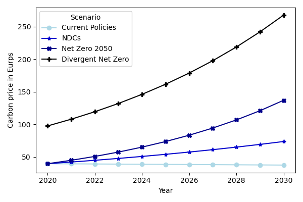
Figure 2: Annual carbon price per scenario

Emissions level	Very High	High	Low	Very Low
Current Policies	4.301	4.301	0.459	0.014
NDCs	6.151	6.151	0.656	0.02
Net Zero 2050	8.883	8.883	0.948	0.03
Divergent Net Zero	19.029	19.029	2.031	0.063

Table 7: Average annual carbon tax on households’ consumption from each sector between 2020 and 2030 (in %)

Eurostat does not provide information on the level of emissions associated with households’ consumption from the Very High Emitting group (see D for more details on groups definition), so we assume that they are the as in High Emitting group. The corresponding tax is thus zero. The highest level of taxation for households’ consumption comes from the High Emitting group (involved for cooking and heating) and from the Low Emitting one (involved for constructing, commuting, and travelling).

Emissions level	Very High	High	Low	Very Low
Current Policies	4.006	1.605	0.413	0.069
NDCs	5.73	2.296	0.591	0.098
Net Zero 2050	8.275	3.315	0.853	0.142
Divergent Net Zero	17.728	7.102	1.827	0.304

Table 8: Average annual carbon tax on firms’ production in each sector between 2020 and 2030 (in %)

On firms’ production side, the Very High Emitting group is the highest taxed (because agriculture and farming emit large amounts of GHG like methane), and is naturally followed by the High Emitting one which emits significant amounts of CO2.

Emissions level / Output	Very High	High	Low	Very Low
Current Policies	5.612	3.945	11.074	2.198
NDCs	8.027	5.642	15.839	3.143
Net Zero 2050	11.592	8.148	22.874	4.539
Divergent Net Zero	24.833	17.454	49.002	9.724

(a) Input: Very High

Emissions level / Output	Very High	High	Low	Very Low
Current Policies	2.059	1.440	4.050	0.806
NDCs	2.945	2.060	5.793	1.153
Net Zero 2050	4.253	2.975	8.366	1.665
Divergent Net Zero	9.111	6.373	17.922	3.566

(b) Input: High

Emissions level / Output	Very High	High	Low	Very Low
Current Policies	0.395	0.277	0.778	0.155
NDCs	2.945	2.06	5.793	1.153
Net Zero 2050	0.815	0.573	1.608	0.319
Divergent Net Zero	1.746	1.227	3.445	0.684

(c) Input: Low

Emissions level / Output	Very High	High	Low	Very Low
Current Policies	0.435	0.307	0.860	0.170
NDCs	0.621	0.439	1.230	0.243
Net Zero 2050	1.923	1.357	3.807	0.752
Divergent Net Zero	0.897	0.633	1.777	0.351

(d) Input: Very Low

Table 9: Average annual carbon tax on firms’ intermediary input from each sector between 2020 and 2030 (in %)

On the taxation of firms’ intermediary consumption, we observe expected patterns. For example, the carbon tax applied on inputs produced by the Very High Emitting sector and consumed by the Low Emitting one is very high. This is explained by the fact that many inputs used by sectors belonging to the Low Emitting group (such as Manufacture of food products, beverages and tobacco products) are produced by Agriculture which belongs to Very High Emitting group. Similar comments can be done for the other sectors. Those results thus show that sectors are not only affected by their own emissions, but also by the emissions from the sectors from which they consume products.

We now calibrate our model on the historical data assuming no carbon tax as detailed in Section 4.2 and perform simulations.

5.4 Output and consumption growth

We compute the mean of the annual consumption growth and related 95% confidence interval for each sector and each scenario. Results are displayed on Figure 3. Additionally, we compute the average annual consumption growth over the ten-year period, as illustrated in Table 10.

Emissions level	Very High	High	Low	Very Low	Total
NDCs	-0.343	-0.115	-0.095	-0.016	-0.140
Net Zero 2050	-1.	-0.323	-0.268	-0.046	-0.399
Divergent Net Zero	-2.119	-0.599	-0.519	-0.098	-0.786

Table 10: Average annual consumption growth evolution with respect to the Current Policies scenario between 2020 and 2030 (in %)

It follows from the Total column in Table 10 that the average annual growth between 2020 and 2030 is decreasing. The Divergent Net Zero is the economic worst case (the best one for the climate) where the carbon ton would cost 395.21€  in 2030. The Current Policies is the economic best case (the worst one for the climate) where the carbon ton would cost 39.05€  in 2030. The difference of annual consumption growth between the worst and the best scenarios is of about $-0.786\%$.

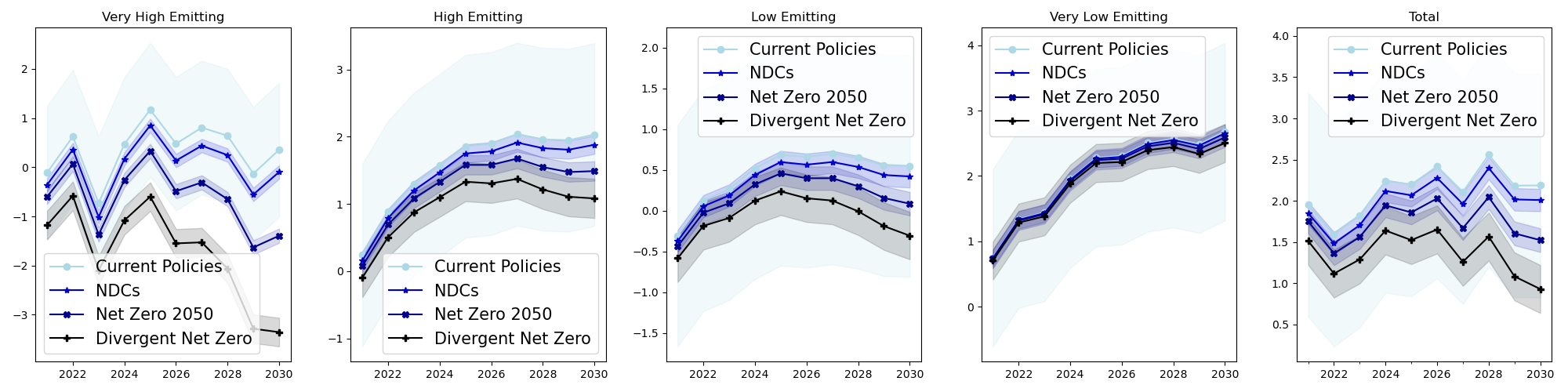
Figure 3: Mean and 95% confidence interval of the annual consumption growth from 2020 to 2030

The four scenarios are clearly discriminating. In the Divergent Net Zero scenario, our model shows, on the last subplot in Figure 3, a drop in consumption growth, with respect to the Current Policies scenario, that starts at 0.438% in 2020 and increases every year until a 1.258% drop is reached in 2030. Cumulatively, from 2020 to 2030, a drop of 7.860% is witnessed.

We can compare this value to 2.270% which is the GDP drop between the Net Zero 2050 and Current Policies scenarios obtained with the REMIND model in [29]. The difference observed with REMIND can be explained by the fact that our model does not specify how the collected carbon taxes are reinvested or redistributed. We could, for example, head the investment towards low-carbon energies, which would have the effect of reducing the tax on these sectors. Moreover, in our model, carbon price is assumed to increase uniformly (which implies that emissions would increase indefinitely - which is not desirable) from 2020 to 2030, while in REMIND an adjustment of the carbon price growth rate is being made in 2025. Furthermore, productivity is totally exogenous in our model while there are exogenous labor productivity and endogenous technological change for green energies in REMIND, which is expected to have a downward effect on the evolution of carbon price. However, we recall that our model has the benefit to be stochastic and multisectoral.

Now, it follows from both Figure 3 and Table 10 that the introduction of carbon taxes is less adverse for the Very Low Emitting and Low Emitting groups than for the High Emitting and Very High Emitting ones. The slowdown is highest for the Very High Emitting group, which was anticipated given that the tax on firms was the highest. However, we can see that, even in the best case scenario, the consumption growth in the Low Emitting group stabilizes or begins to decline. It is probably because we are working on French data and the industrial production in the French economy structurally decreases. Moreover, the slowdown could be accelerated by the climate transition, not only because this sector emits GHG, but also because its intermediary inputs are from High Emitting and Very High Emitting sectors. On the other hand, the Very Low Emitting sector continues its strong growth because it emits less and because France is driven by the service industry. Finally, the consumption in the two most polluting sectors suffers from a slowdown higher than the whole consumption slowdown and lower than in the two least polluting ones.

5.5 Firm Valuation

Here, we consider a representative firm characterized by its cashflow $F_{t_{\circ}-1}$ at $t_{\circ}-1$, with standard deviation $\sigma_{\mathfrak{b}}$ and by the contribution $\mathfrak{a}$ of sectoral consumption growth to its cash flows growth. We would like to know how the value of this company evolves during the transition period and with the carbon price introduced in the economy. Consider $F_{t_{\circ}-1}=\text{€{1,000,000}}$, $\sigma_{\mathfrak{b}}=5.0\%$, $\mathfrak{a}=[0.25,0.25,0.25,0.25]$ (each sector has the same contribution to the growth of the cash flows of the firm), the interest rate $r=5\%$. For $M=1000$ simulations of the productivity processes $(\Theta_{t},\mathcal{A}_{t})_{t_{\circ}\leq t\leq t_{\star}}$, we compute the firm value using (2.7). We can analyze both the average evolution of the firm value per year and per scenario (Figure 4) and the empirical distribution of the firm value per scenario (Figure 5).

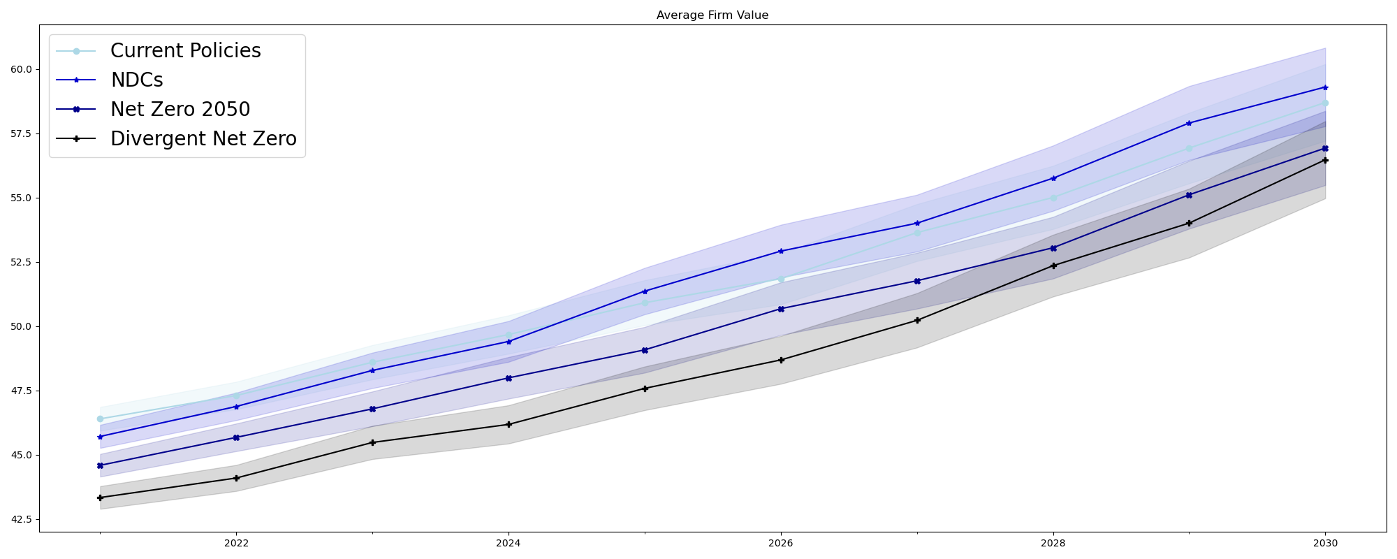
Figure 4: Average annual firm value per scenario in million euros per year

We see that even if the value of the firm grows each year, this growth is affected by the severity of the transition scenario. The presence of the carbon tax in the economy clearly reduces the firm value.

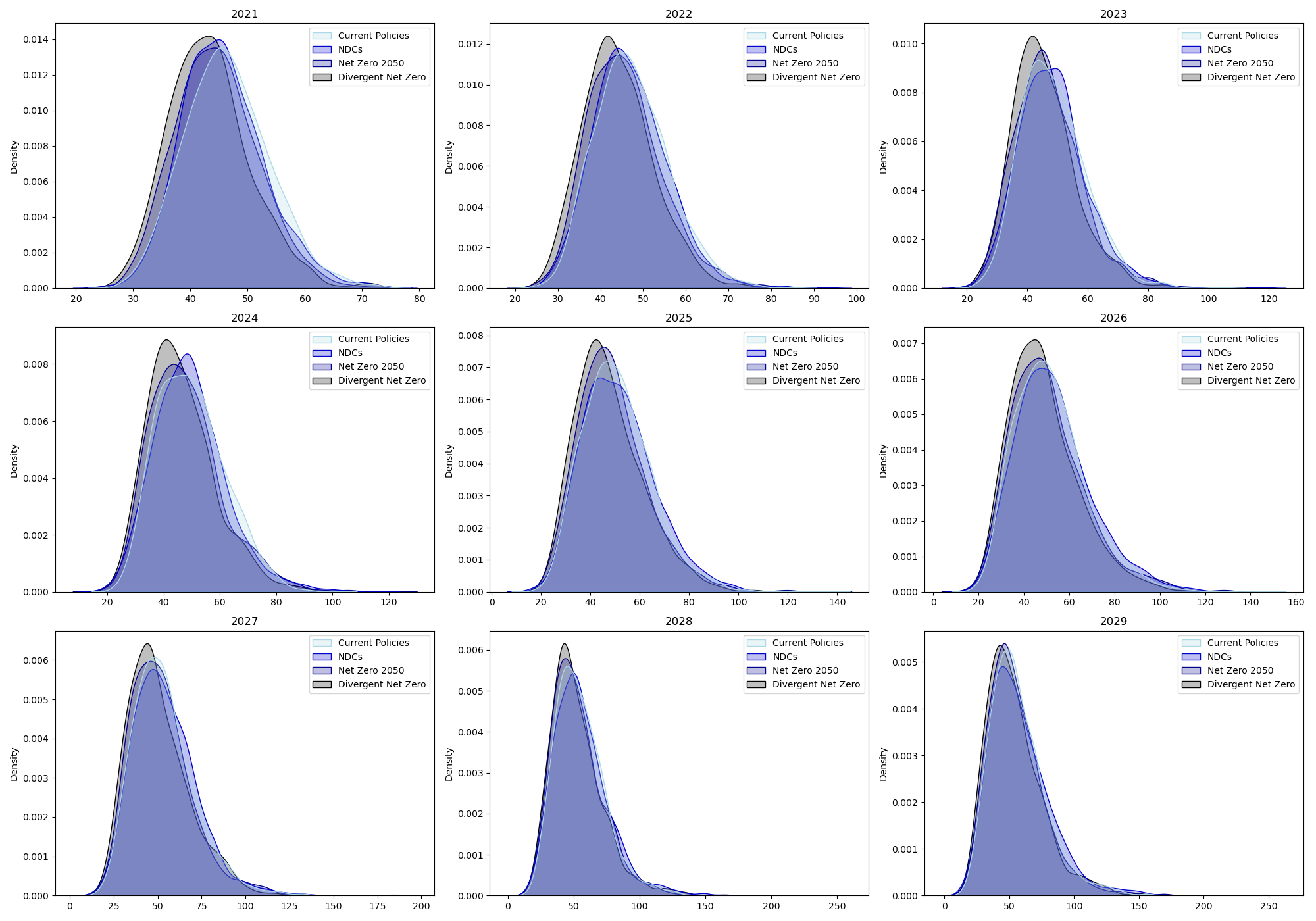
Figure 5: Firm value distribution per scenario and per year

The introduction of the transition scenario distorts the density function of the firm value, and in particular, moves it to the left.

5.6 Credit Risk

Consider a fictitious portfolio of $N=12$ firms described in Table 11 below. This choice is made to ease the reproducibility of the result since the default data are proprietary data of BPCE. Note that the growths in the cash flows of Firm $2$, $4$, $6$, and $8$ are respectively driven by the Very High Emitting, High Emitting, Low Emitting, and Very Low Emitting groups.

n°	1	2	3	4	5	6	7	8	9	10	11	12
$\sigma_{\mathfrak{b}^{n}}$	0.05	0.05	0.06	0.06	0.07	0.07	0.08	0.08	0.09	0.09	0.10	0.10
$F_{0}^{n}$	1.0	1.0	1.0	1.0	1.0	1.0	1.0	1.0	1.0	1.0	1.0	1.0
$B^{n}$	3.41	3.14	3.47	3.83	3.49	3.19	3.36	3.54	4.21	3.01	2.46	2.45
$\mathfrak{a}^{n}$(Very High)	0.25	1.0	0.5	0.0	0.0	0.0	0.0	0.0	0.25	0.25	0.25	0.75
$\mathfrak{a}^{n}$(High)	0.25	0.0	0.5	1.0	0.5	0.0	0.0	0.0	0.50	0.50	0.25	-0.16
$\mathfrak{a}^{n}$(Low)	0.25	0.0	0.0	0.0	0.5	1.0	0.5	0.0	0.25	0.25	0.50	0.16
$\mathfrak{a}^{n}$(Very Low)	0.25	0.0	0.0	0.0	0.0	0.0	0.5	1.0	0.25	-0.25	-0.50	-0.16

Table 11: Characteristics of the portfolio

5.6.1 Probabilities of default (PD)

We use the parameters of the portfolio and firms as detailed in Table 11 to compute annual PDs over ten years using the closed-form formulae (4.7). We then report, in Figure 6, the average annual PD and its annual evolution.

The remarks raised for the consumption growth remain valid, only the monotony changes: we can clearly distinguish the fourth various climate transition scenario. The probability of default grows each year, which is consistent as uncertainty increases with time. Even in the Current Policies scenario, the PD goes from 5.970% in 2021 to 7.024% in 2030.

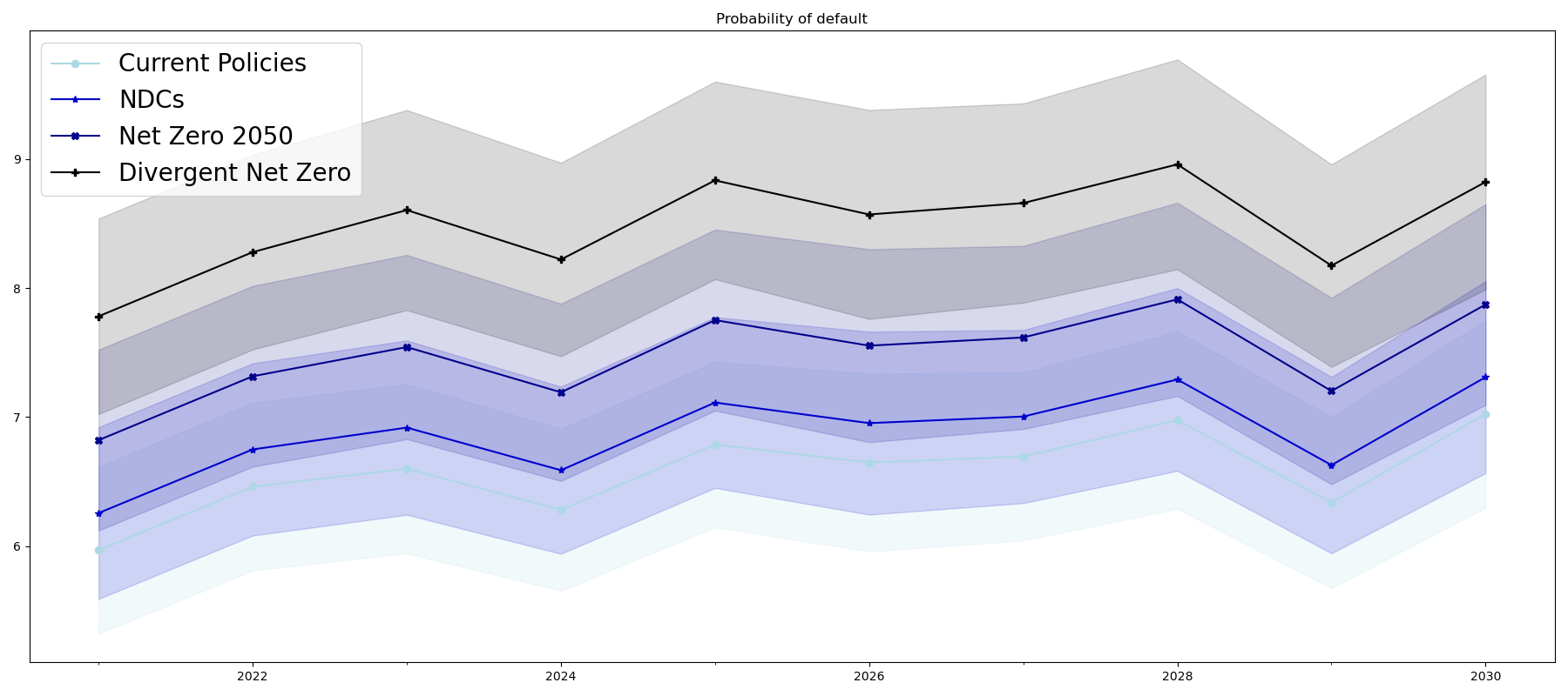
Figure 6: Average annual probability of default of the portfolio per scenario and year in %

Moreover, the increase is emphasized when the transition scenario gets tougher from an economic point of view. Between the worst-case (Divergent Net Zero) scenario and the best-case (Current Policies) one, the difference in average default probability reaches 1.911% in 2030. Over the next 10 years, the annual average PD for the Current Policies scenario is 6.579%, for the NDCs scenario is 6.882%, for the Net Zero 2050 scenario is 7.478%, and for the Divergent Net Zero scenario is 8.490%. It is no surprise that the introduction of a carbon tax increases the portfolio’s average probability of default.

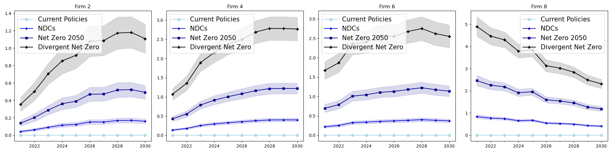
Figure 7: Average annual probability of default per scenario and per firm

In Figure 7 above, we can also observe that, for each company, the evolution of PD depends on the sector that is at the origin of the growth of its cash flows. As expected, the PD grows throughout the years, and the growth is even more abrupt when the sector to which the company belongs to is polluting.

5.6.2 Expected and unexpected losses

We compute the EL and UL using (4.8) and (4.9), assuming that LGD and EAD are constant over the years and $\mathrm{LGD}^{n}=45\%$ and $\mathrm{EAD}^{n}=\text{€{1 million}}$ for each firm $n$ described in Table 11. The annual exposure of the notional portfolio of $N=12$ firms thus remains fixed and is equal to €12 millions. We then express losses as a percentage of the firm’s or portfolio’s exposure. Table 12 and Table 13 show the average annual EL and UL.

Emissions level	Firm 2	Firm 4	Firm 6	Firm 8	Portfolio
Current Policies	0.19	0.387	0.593	0.613	2.898
NDCs	0.204	0.413	0.609	0.616	3.030
Net Zero 2050	0.234	0.464	0.639	0.62	3.291
Divergent Net Zero	0.327	0.539	0.684	0.627	3.733

Table 12: Average annual EL as a percentage of exposure

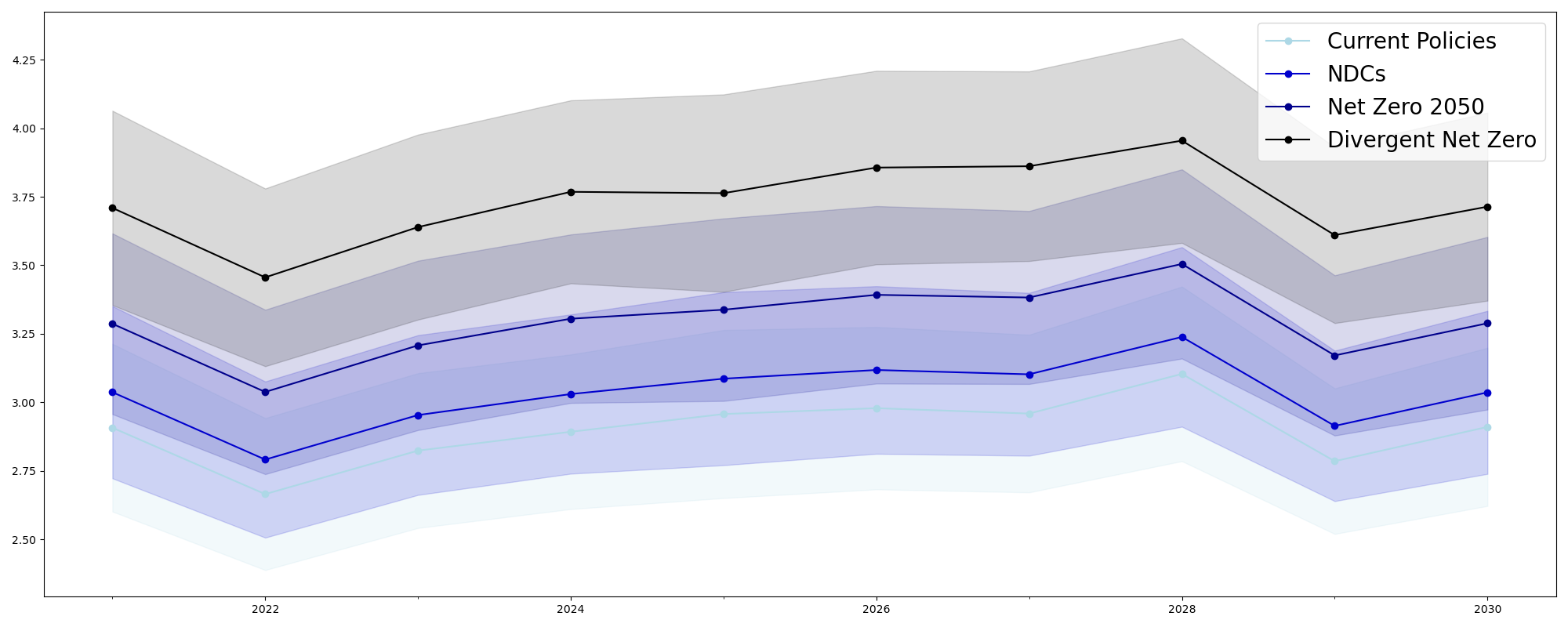
Figure 8: EL of the portfolio in % of the exposure per scenario and per year.

We observe in Table 12 and Figure 8 that, as expected (notably because the LGD is not stressed), the different scenarios remain clearly differentiated for the EL. EL as a percentage of the portfolio’s exposure increases with the year and the carbon price/taxes. For the portfolio as a whole, we see that the average annual EL increases by 62% between the two extreme scenarios. Moreover, still focusing on the two extreme scenarios, the average annual EL increases by 72% for Firm 2 belonging to the Very High Emitting group while it increases by 2% for Firm 8 belonging to the Very Low Emitting group.

EL being covered by the provisions coming from the fees charged to the client, an increase in EL implies an increase in credit cost.

Therefore, somehow, companies from the most polluting sectors will be charged more than those from the least polluting sectors.

Emissions level	Firm 2	Firm 4	Firm 6	Firm 8	Portfolio
Current Policies	0.895	0.27	0.205	0.368	1.683
NDCs	0.941	0.282	0.209	0.369	1.755
Net Zero 2050	1.031	0.305	0.215	0.371	1.895
Divergent Net Zero	1.19	0.336	0.224	0.373	2.133

Table 13: Average annual UL as a percentage of exposure

Figure 9: UL of the portfolio in % of the exposure per scenario and per year

Similarly for the UL, we observe the difference between the scenarios from Table 13 and Figure 9. For the portfolio as a whole, we see that the average annual UL increases by 27% between the two extreme scenarios. Moreover, still focusing on the two extreme scenarios, the average annual UL increases by 32% for Firm 2 belonging to the Very High Emitting group while it increases by 2% for Firm 8 belonging to the Very Low Emitting group.

UL being covered by the economic capital coming from the capital gathered by the shareholders, an increase in UL implies a decrease in the bank’s profitability. Therefore, in some way, granting loans to companies from the most polluting sectors will affect banks more negatively than doing so to companies from the least polluting sectors.

We therefore observe that the introduction of a carbon price will not only increase the banking fees charged to the client (materialized by the provisions via the expected loss) but will also reduce the bank’s profitability (via the economic capital that is calculated from the unexpected loss).

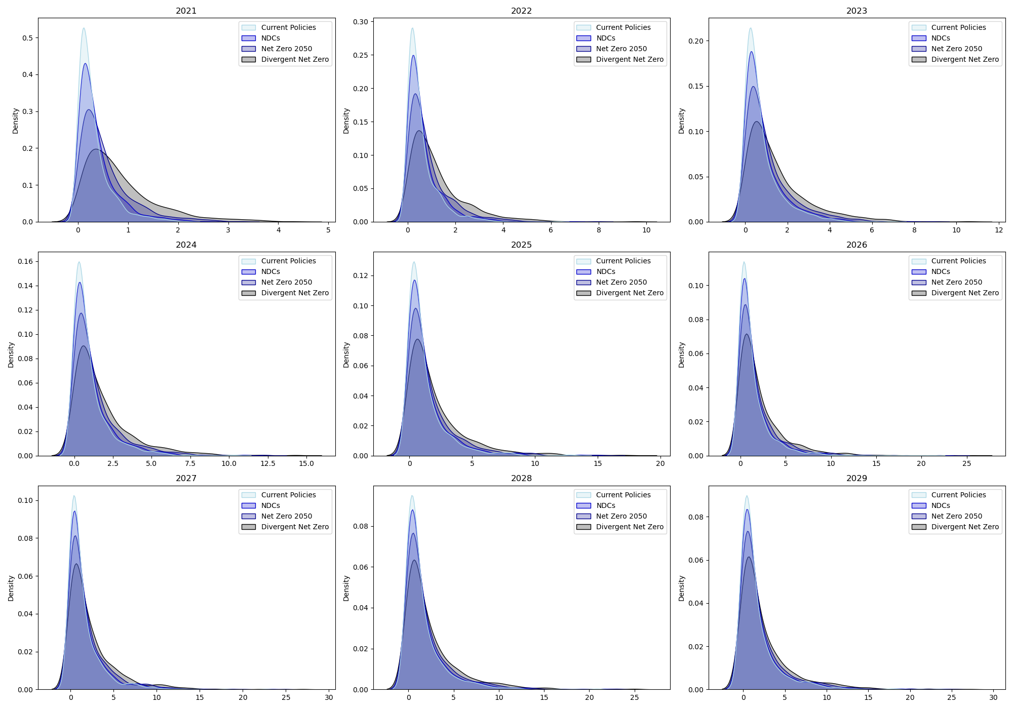
Figure 15: Annual EL distribution per scenario

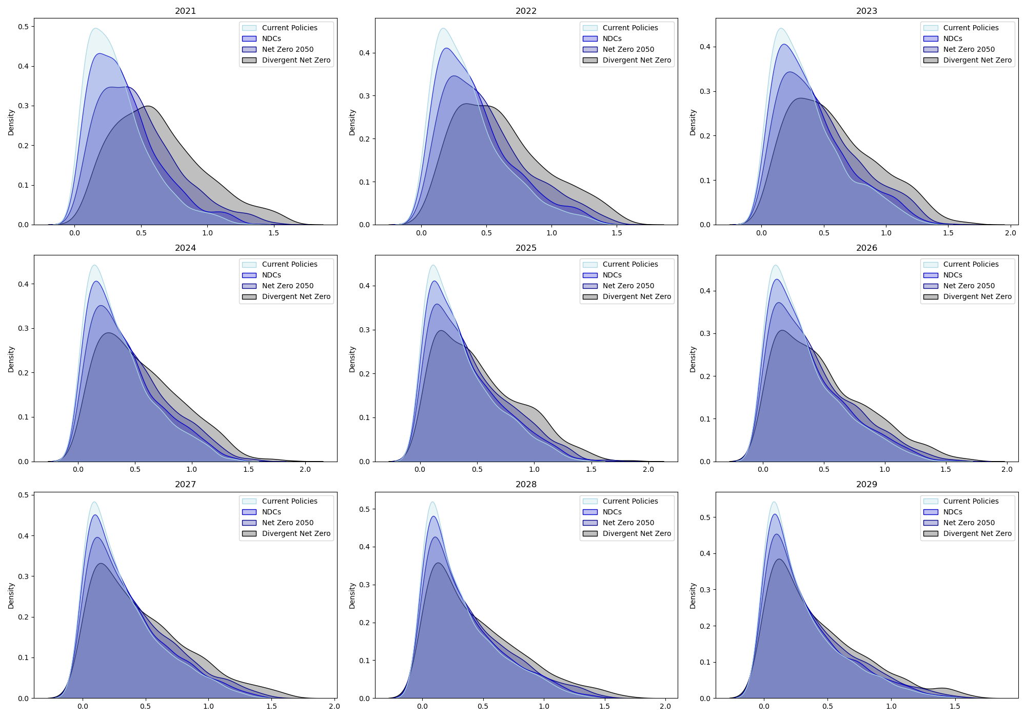
Figure 16: Annual UL distribution per scenario

Finally, for more in-depth analysis, Figure 15 (respectively Figure 16) shows the distortions of the distribution of EL (respectively UL) per scenario and per year.

5.6.3 Losses’ sensitivities to carbon taxes

Finally, we compute the sensitivity of our portfolio losses to carbon taxes using (4.10). Since the scenarios are deterministic, this quantity allows us to measure some form of model uncertainty. Indeed, for a given scenario, it allows to capture the level by which the computed loss would vary should that assumed deterministic scenario deviate by a certain percentage. For each time $t$, we choose the direction $\mathfrak{U}\in([0,1)^{I}\times[0,1)^{I\times I}\times[0,1)^{I})^{t_{\star}+1}$ which is equal to $1$ at $t$ and $0$ everywhere else, and a step $\vartheta=1\%$. A carbon price change of 1% will cause a change in EL of $\widehat{\Gamma}^{N,T}_{t,\mathfrak{d}}(\mathrm{EL})$ and a change in UL of $\widehat{\Gamma}^{N,T}_{t,\mathfrak{d},\alpha}(\mathrm{UL})$. We report the results in Table 14 and Table 15.

For example, over the next ten years, if the price of carbon varies by 1% around the scenario NDCs, the EL will vary by $1.402$% while the UL will change by $1.148$% around this scenario.

Emissions level	Firm 2	Firm 4	Firm 6	Firm 8	Portfolio
Current Policies	1.561	1.581	1.191	0.827	1.280
NDCs	1.777	1.687	1.261	0.904	1.402
Net Zero 2050	2.142	1.864	1.386	1.035	1.631
Divergent Net Zero	2.668	2.096	1.562	1.215	1.973

Table 14: Average annual EL sensitivity to carbon price in %

Emissions level	Firm 2	Firm 4	Firm 6	Firm 8	Portfolio
Current Policies	1.299	1.290	1.042	0.547	1.135
NDCs	1.463	1.365	1.102	0.583	1.148
Net Zero 2050	1.726	1.485	1.206	0.634	1.197
Divergent Net Zero	2.070	1.632	1.352	0.681	1.472

Table 15: Average annual UL sensitivity to carbon price in %

The greater the sensitivity, the more polluting the sector is. This is to be expected as carbon taxes are higher in these sectors. In addition, the sensitivity of the portfolio is smaller than that in the most polluting sectors, and greater than that in the least polluting ones. Finally, we notice that the variation of the EL is slightly more sensitive than the variation of the UL. This means that the bank’s provisions will increase a bit more than the bank’s capital, or that the growth of the carbon taxes will impact customers more than shareholders.

Conclusion

In this work, we study how the introduction of carbon taxes would propagate in a credit portfolio. To this aim, we first build a dynamic stochastic multisectoral model in which we introduce carbon taxes calibrated on sectoral greenhouse gases emissions. We later use the Discounted Cash Flows methodology to compute the firm value and introduce the latter in the Merton model to project $\mathrm{PD}$, $\mathrm{EL}$ and $\mathrm{UL}$. We finally introduce losses’ sensitivities to carbon taxes to measure the uncertainty of the losses to the transition scenarios. This work opens the way to numerous extensions mobilizing diverse and varied mathematical tools. In the climate-economic model, exogenous and deterministic scenarios as well as heterogeneous agents are assumed while one could consider agent-based or mean-field games models where a central planner decides on the carbon taxes and agents (companies or households) optimize production, prices, and consumption according to the tax level. In the credit risk part, the LGD is assumed to be deterministic, constant, and independent of the carbon taxes. In our forthcoming research, we will analyze how the LGD is affected by the stranding of assets. We furthermore assume that $\mathrm{EAD}$ and thus bank balance sheets remain static over the years while the transition will require huge investments. One could thus introduce capital in the model. Finally, we have adopted a sectoral view, while one could alternatively assess the credit risk at the counterpart level and thus penalize or reward companies according to their individual and not sectoral emissions.

Appendix A Vector Autoregressive Model (VAR):

Detailed proofs in Hamilton [23], and Kilian and Lütkepohl [25]. Assume that $(\Theta_{t})_{t\in\mathbb{N}}$ follows a VAR, i.e. for all $t\in\mathbb{N}^{*}$,

$$\Theta_{t}=\mu+\Gamma\Theta_{t-1}+\mathcal{E}_{t},\quad\text{where for}\quad t\in\mathbb{Z},\quad\mathcal{E}_{t}\sim\mathcal{N}(\mathbf{0},\Sigma)$$ (A.1)

with $\mu\in\mathbb{R}^{I}$ and where the matrix $\Gamma\in\mathbb{R}^{I\times I}$ has eigenvalues all strictly less than $1$ in absolute value. We have the following result that can be easily show in VAR’s literature.

• $(\Theta_{t})_{t\in\mathbb{N}}$ is weak-stationary.

• If $\Theta_{0}\sim\mathcal{N}(\overline{\mu},\overline{\Sigma})$ with $\overline{\mu}:=(\mathbf{I}_{I}-\Gamma)^{-1}\mu$, and $\mathrm{vec}(\overline{\Sigma})=(\mathbf{I}_{I\times I}-\Gamma\bigotimes\Gamma)^{-1}\mathrm{vec}(\Sigma)$, then for $t\in\mathbb{Z}$, $\mathcal{E}_{t}\sim\mathcal{N}(\mathbf{0},\Sigma)$ with $\Sigma\in\mathbb{R}^{I\times I}$.

• For $t,T\in\mathbb{N}$, we note $\Upsilon_{t}:=\sum_{v=0}^{t}\Gamma^{v}$, then

  $$\sum_{u=1}^{T}\sum_{v=1}^{u}\Gamma^{u-v}\mathcal{E}_{t+v}=\sum_{u=1}^{T}\Upsilon_{T-u}\mathcal{E}_{t+u},$$

• For $t,u\in\mathbb{N}$,

  $$\Theta_{t}=\overline{\mu}+\sum_{v=1}^{\infty}\Gamma^{v}\mathcal{E}_{t-v}\qquad\text{and}\qquad\Theta_{t+T}=\Gamma^{T}\Theta_{t}+\Upsilon_{T-1}\mu+\sum_{v=1}^{T}\Gamma^{T-v}\mathcal{E}_{t+v}.$$ (A.2)

• For $t,T\in\mathbb{N}$,

  $$\left(\sum_{u=1}^{T}\Theta_{t+u}\middle|\Theta_{t}\right)\sim\mathcal{N}\left(\Gamma\Upsilon_{T-1}\Theta_{t}+\left(\sum_{u=1}^{T}\Upsilon_{u-1}\right)\mu,\sum_{u=1}^{T}\Upsilon_{T-u}\Sigma(\Upsilon_{T-u})^{\top}\right),$$ (A.3)

  and in particular $\left(\Theta_{t+1}\middle|\Theta_{t}\right)\sim\mathcal{N}\left(\mu+\Gamma\Theta_{t},\Sigma\right)$.

Appendix B Proofs

B.1 Existence condition of the Firm Value

Proof of Proposition 2.5.

Let $t\in\mathbb{N}$, $n\in\{1,\ldots,N\}$. For $s>0$, from Assumption 2.4, we observe that

$$F^{n}_{t+s}=F^{n}_{t}\exp\left(\sum_{u=1}^{s}w^{n}_{t+u}\right).$$ (B.1)

Let $K\in\mathbb{N}^{*}$ and define

$$V^{n,K}_{t} :=\mathbb{E}_{t}\left[\sum_{s=0}^{K}e^{-rs}F^{n}_{t+s}\right].$$ (B.2)

We now show that $\lim_{K\rightarrow+\infty}V^{n,K}$ exists, in particular that $\mathbb{E}_{t}\left[e^{-rs}F^{n}_{t+s}\right]$ is summable. To this end, we first observe that

$$V^{n,K}_{t}=F^{n}_{t}\left(1+\sum_{s=1}^{K}e^{-rs}\mathbb{E}_{t}\left[\exp\left(\sum_{u=1}^{s}w^{n}_{t+u}\right)\right]\right).$$

We now give an upper bound for $\|\exp\left(\sum_{u=1}^{s}w^{n}_{t+u}\right)\|_{p}$ for some $p>1$. We observe that, using (2.2),

$$\sum_{u=1}^{s}w^{n}_{t+u}=\mathfrak{a}^{n\cdot}\left(\sum_{u=1}^{s}\Theta_{t+u}+v(\mathfrak{d}_{t+s})-v(\mathfrak{d}_{t})\right)+\sum_{u=1}^{s}\mathfrak{b}^{n}_{t+u}.$$ (B.3)

From Assumption 1.1 and (1.3), it follows

$$\Theta_{t+u}=\overline{\mu}+\varepsilon\left(\Gamma^{u}\mathcal{Z}_{t}+\sum_{v=1}^{u}\Gamma^{u-v}\mathcal{E}_{t+v}\right).$$

We define $\Upsilon_{k}:=\sum_{v=0}^{k}\Gamma^{v}$ and observe that

$$|\Upsilon_{k}|\leq(1-|\Gamma|)^{-1}\;.$$ (B.4)

Since

$$\sum_{u=1}^{s}\sum_{v=1}^{u}\Gamma^{u-v}\mathcal{E}_{t+v}=\sum_{v=1}^{s}\Upsilon_{s-v}\mathcal{E}_{t+v},$$ (B.5)

we compute

$$\sum_{u=1}^{s}\Theta_{t+u}=\overline{\mu}s+\varepsilon\Gamma\Upsilon_{s-1}\mathcal{Z}_{t}+\varepsilon\sum_{v=1}^{s}\Upsilon_{s-v}\mathcal{E}_{t+v}.$$

Then (B.3) reads

$$\sum_{u=1}^{s}w^{n}_{t+u}=\varepsilon\mathfrak{a}^{n\cdot}\Gamma\Upsilon_{s-1}\mathcal{Z}_{t}+s\mathfrak{a}^{n\cdot}\overline{\mu}+\varepsilon\sum_{v=1}^{s}\mathfrak{a}^{n\cdot}\Upsilon_{s-v}\mathcal{E}_{t+v}+\mathfrak{a}^{n\cdot}\left(v(\mathfrak{d}_{t+s})-v(\mathfrak{d}_{t})\right)+\sum_{u=1}^{s}\mathfrak{b}^{n}_{t+u}.$$

Observe that under Assumption 1.3, there exists a constant $\mathfrak{C}>0$ such that

$$\sup_{n,s,t}\exp\left(\mathfrak{a}^{n\cdot}\left(v(\mathfrak{d}_{t+s})-v(\mathfrak{d}_{t})\right)\right)\leq\mathfrak{C}\,.$$ (B.6)

Thus, using the independence of $\mathcal{Z}_{t},(\mathcal{E}_{t+v})_{v\geq 1},(\mathfrak{b}^{n}_{t+v})_{v\geq 1}$, we obtain

$$\mathbb{E}_{t}\left[\exp\left(p\sum_{u=1}^{s}w^{n}_{t+u}\right)\right]\leq \mathfrak{C}^{p}\exp\Big{(}p\varepsilon\mathfrak{a}^{n\cdot}\Gamma\Upsilon_{s-1}\mathcal{Z}_{t}+ps\mathfrak{a}^{n\cdot}\overline{\mu}\Big{)}\mathbb{E}\left[\exp\left(p\varepsilon\sum_{v=1}^{s}\mathfrak{a}^{n\cdot}\Upsilon_{s-v}\mathcal{E}_{t+v}+p\sum_{u=1}^{s}\mathfrak{b}^{n}_{t+u}\right)\right].$$ (B.7)

Since

$$\mathbb{E}\left[\exp\left(p\sum_{u=1}^{s}\mathfrak{b}^{n}_{t+u}\right)\right]=\exp\left(\frac{p^{2}}{2}s\sigma_{\mathfrak{b}^{n}}^{2}\right),$$ (B.8)

we compute

$$\mathbb{E}\left[\exp\left(p\varepsilon\mathfrak{a}^{n\cdot}\Upsilon_{s-v}\mathcal{E}_{t+v}\right)\right]=\exp\left(\frac{\varepsilon^{2}p^{2}}{2}|\mathfrak{a}^{n\cdot}\Upsilon_{s-v}\sqrt{\Sigma}|^{2}\right)\leq\exp\left(\frac{\varepsilon^{2}p^{2}}{2}|\mathfrak{a}^{n\cdot}|^{2}|\sqrt{\Sigma}|^{2}(1-|\Gamma|)^{-2}\right).$$ (B.9)

One could also have found above a finer upper bound. Combining (B.8)-(B.9) with (B.7), we obtain

$$\mathbb{E}_{t}\left[\exp\left(p\sum_{u=1}^{s}w^{n}_{t+u}\right)\right]\leq\mathfrak{C}^{p}\exp\left(p\varepsilon\mathfrak{a}^{n\cdot}\Gamma\Upsilon_{s-1}\mathcal{Z}_{t}+p^{2}\rho s\right).$$

Using similar computations as above, we also get (because $\Upsilon_{s-1}$ and $\mathcal{Z}_{t}$ is stationary and Gaussian)

$$\mathbb{E}\left[\exp\left(p\varepsilon\mathfrak{a}^{n\cdot}\Gamma\Upsilon_{s-1}\mathcal{Z}_{t}\right)\right]\leq C_{p},$$ (B.10)

and hence

$$\left\|\exp\left(\sum_{u=1}^{s}w^{n}_{t+u}\right)\right\|_{p}\leq C_{p}e^{p\rho s}.$$

Under (2.5), we then obtain

$$\sum_{s\geq 0}e^{-rs}\left\|\exp\left(\sum_{u=1}^{s}w^{n}_{t+u}\right)\right\|_{p}<+\infty,$$ (B.11)

for some $p>1$. Set $1<\tilde{p}:=\frac{p}{1+\epsilon}$, for $\epsilon>0$ small enough. Then, using Hölder’s inequality (with $\frac{1}{\tilde{p}}=\frac{1}{p}+\frac{1}{p/\epsilon}$),

$$\mathbb{E}\left[|V^{n,K}_{t}|^{\tilde{p}}\right]\leq C_{p}\mathbb{E}\left[|F_{t}^{n}|^{\frac{p}{\epsilon}}\right]<+\infty,$$

since $\|F^{n}_{t}\|_{q}<\infty$ for any $q\geq 1$. ∎

B.2 Conditional distribution of the firm value

Proof of Remark 2.9.

Let $t,T\geq 1$, we have from (2.7),

$$\begin{split}\mathcal{V}^{n}_{t+T}&=F^{n}_{0}\mathfrak{R}^{n}_{t+T}(\mathfrak{d})\exp{\left(\mathfrak{a}^{n\cdot}(\mathcal{A}^{\circ}_{t+T}-v(\mathfrak{d}_{0}))\right)}\exp\left(\sum_{u=1}^{t+T}\mathfrak{b}^{n}_{u}\right)\\ &=F^{n}_{0}\mathfrak{R}^{n}_{t+T}(\mathfrak{d})\exp{\left(-\mathfrak{a}^{n\cdot}v(\mathfrak{d}_{0})\right)}\exp{\left(\mathfrak{a}^{n\cdot}\mathcal{A}^{\circ}_{t+T}\right)}\exp\left(\mathcal{W}_{t+T}^{n}\right)\end{split}$$

But $\mathcal{A}^{\circ}_{t+T}=\mathcal{A}^{\circ}_{t}+\sum_{u=t+1}^{t+T}\Theta_{u}$, then

$$\begin{split}\mathcal{V}^{n}_{t+T}&=F^{n}_{0}\mathfrak{R}^{n}_{t+T}(\mathfrak{d})\exp{\left(\mathfrak{a}^{n\cdot}(\mathcal{A}^{\circ}_{t}-v(\mathfrak{d}_{0}))\right)}\exp{\left(\mathfrak{a}^{n\cdot}\sum_{u=t+1}^{t+T}\Theta_{u}\right)}\exp\left(\mathcal{W}^{n}_{t+T}\right)\\ &=F^{n}_{0}\mathfrak{R}^{n}_{t+T}(\mathfrak{d})\exp{\left(\mathfrak{a}^{n\cdot}(\mathcal{A}^{\circ}_{t}-v(\mathfrak{d}_{0}))\right)}\exp{\left(\mathfrak{a}^{n\cdot}\sum_{u=1}^{T}\Theta_{t+u}+\mathcal{W}^{n}_{t+T}\right)}.\end{split}$$

But recall from Remark 1.2 and A, for all $u\in\{1,\ldots,T\}$,

$$\Theta_{t+u}=\Gamma^{u}\Theta_{t}+\Upsilon_{u-1}\mu+\varepsilon\sum_{v=1}^{u}\Gamma^{u-v}\mathcal{E}_{t+v},$$

then

$$\sum_{u=1}^{T}\Theta_{t+u}=\sum_{u=1}^{T}\Gamma^{u}\Theta_{t}+\sum_{u=1}^{T}\Upsilon_{u-1}\mu+\varepsilon\sum_{u=1}^{T}\sum_{v=1}^{u}\Gamma^{u-v}\mathcal{E}_{t+v}=\Gamma\Upsilon_{T-1}\Theta_{t}+\left(\sum_{u=1}^{T}\Upsilon_{u-1}\right)\mu+\varepsilon\sum_{v=1}^{T}\Upsilon_{T-v}\mathcal{E}_{t+v}.$$

From Assumptions 1.1 and 2.1, we have

$$\left(\sum_{u=1}^{T}\mathfrak{a}^{n\cdot}\Theta_{t+u}+\mathcal{W}^{n}_{t+T}\middle|\mathcal{G}_{t}\right)\sim\mathcal{N}\left(\mathfrak{a}^{n\cdot}\Gamma\Upsilon_{T-1}\Theta_{t}+\mathfrak{a}^{n\cdot}\left(\sum_{u=1}^{T}\Upsilon_{u-1}\right)\mu,\varepsilon^{2}\sum_{u=1}^{T}(\mathfrak{a}^{n\cdot}\Upsilon_{T-u})\Sigma(\Upsilon_{T-u}\mathfrak{a}^{n\cdot})^{\top}+\sigma_{\mathfrak{b}^{n}}^{2}(t+T)\right),$$

and the conclusion follows. ∎

B.3 Convergence of $(\mathcal{V}^{n}_{t}-V^{n}_{t})/F^{n}_{t}$o zero

Proof of Proposition 2.10.

For $K\in\mathbb{N}^{*}$, recall the expressions of $V^{n,K}_{t}$ in (B.2) and $\mathcal{V}^{n,K}_{t}$ in (2.10) and note that

$$\mathbb{E}\left[\left|\frac{V^{n}_{t}}{F^{n}_{t}}-\frac{\mathcal{V}^{n}_{t}}{F^{n}_{t}}\right|\right]\leq\mathbb{E}\left[\left|\frac{V^{n}_{t}}{F^{n}_{t}}-\frac{V^{n,K}_{t}}{F^{n}_{t}}\right|\right]+\mathbb{E}\left[\left|\frac{V^{n,K}_{t}}{F^{n}_{t}}-\frac{\mathcal{V}^{n,K}_{t}}{F^{n}_{t}}\right|\right]+\mathbb{E}\left[\left|\frac{\mathcal{V}^{n,K}_{t}}{F^{n}_{t}}-\frac{\mathcal{V}^{n}_{t}}{F^{n}_{t}}\right|\right]\,.$$ (B.12)

Using Hölder’s inequality and Proposition 2.5, one gets that the first term in the right hand side of the above inequality goes to $zero$ as $K$ goes to $+\infty$. Similarly, using Hölder’s inequality and (the beginning of the proof of) Lemma 2.7, one shows that the last term in the right hand side of the above inequality goes to zero as $K$ goes to infinity. It remains thus to study the middle term to obtain the desired result. Observe that

$$\frac{V^{n,K}_{t}-\mathcal{V}^{n,K}_{t}}{F^{n}_{t}}=\left(\sum_{s=1}^{K}e^{-rs}\mathbb{E}_{t}\left[\exp\left(s\mathfrak{a}^{n\cdot}\overline{\mu}+\mathfrak{a}^{n\cdot}(v(\mathfrak{d}_{t+s})-v(\mathfrak{d}_{t}))+\sum_{u=1}^{s}\mathfrak{b}^{n}_{t+u}\right)\Delta_{s}\right]\right),$$

with

$$\Delta_{s}:=\exp\left\{\varepsilon\sum_{u=1}^{s}\mathfrak{a}^{n\cdot}\mathcal{Z}_{t+u}\right\}-1,$$ (B.13)

using (B.3) and (1.3). We first compute, by independence,

$$\begin{split}&\left|\mathbb{E}_{t}\left[\exp\left(s\mathfrak{a}^{n\cdot}\overline{\mu}+\mathfrak{a}^{n\cdot}(v(\mathfrak{d}_{t+s})-v(\mathfrak{d}_{t}))+\sum_{u=1}^{s}\mathfrak{b}^{n}_{t+u}\right)\Delta_{s}\right]\right|\\ &=\mathbb{E}\left[\exp\left(s\mathfrak{a}^{n\cdot}\overline{\mu}+\mathfrak{a}^{n\cdot}(v(\mathfrak{d}_{t+s})-v(\mathfrak{d}_{t}))+\sum_{u=1}^{s}\mathfrak{b}^{n}_{t+u}\right)\right]\left|\mathbb{E}_{t}\left[\Delta_{s}\right]\right|\\ &\leq\mathfrak{C}\exp\left(s\mathfrak{a}^{n\cdot}\overline{\mu}+\frac{1}{2}s\sigma_{\mathfrak{b}^{n}}^{2}\right)\mathbb{E}_{t}\left[|\Delta_{s}|\right],\end{split}$$

using (B.6). We then obtain

$$\|(V^{n,K}_{t}-\mathcal{V}^{n,K}_{t})/F^{n}_{t}\|_{1}\leq\left(\sum_{s=1}^{K}\mathfrak{C}e^{\varrho_{n}s}\mathbb{E}\left[|\Delta_{s}|\right]\right),$$

where $\varrho_{n}$ is defined in Lemma 2.7. We can rewrite (B.13) as

$$\Delta_{s}=\varepsilon\int_{0}^{1}\exp{\left(\varepsilon\lambda\sum_{u=1}^{s}\mathfrak{a}^{n\cdot}\mathcal{Z}_{t+u}\right)}\sum_{u=1}^{s}\mathfrak{a}^{n\cdot}\mathcal{Z}_{t+u}d\lambda.$$

For $p>1$, using Hölder’s inequality, we deduce from the previous expression

$$\mathbb{E}\left[|\Delta_{s}|\right]\leq\varepsilon\mathbb{E}\left[\left|\int_{0}^{1}\exp{\left(\varepsilon\lambda\sum_{u=1}^{s}\mathfrak{a}^{n\cdot}\mathcal{Z}_{t+u}\right)}d\lambda\right|^{p}\right]^{\frac{1}{p}}\mathbb{E}\left[\left|\sum_{u=1}^{s}\mathfrak{a}^{n\cdot}\mathcal{Z}_{t+u}\right|^{q}\right]^{\frac{1}{q}},$$ (B.14)

with $q$ the conjugate exponent to $p$.

We first compute by convexity

$$\mathbb{E}\left[\left|\sum_{u=1}^{s}\mathfrak{a}^{n\cdot}\mathcal{Z}_{t+u}\right|^{q}\right]\leq s^{q-1}\sum_{u=1}^{s}\mathbb{E}\left[\left|\mathfrak{a}^{n\cdot}\mathcal{Z}_{t+u}\right|^{q}\right]\leq C_{q}s^{q},$$

where the last inequality follows since $\mathcal{Z}_{t+u}\sim\mathcal{N}(0,\overline{\Sigma})$.

We now turn to the first term in the right hand side of (B.14),

Using Jensen’s inequality, we have

$$\mathbb{E}\left[\left|\int_{0}^{1}\exp{\left(\varepsilon\lambda\sum_{u=1}^{s}\mathfrak{a}^{n\cdot}\mathcal{Z}_{t+u}\right)}d\lambda\right|^{p}\right]\leq\int_{0}^{1}\mathbb{E}\left[\exp{\left(\varepsilon\lambda p\sum_{u=1}^{s}\mathfrak{a}^{n\cdot}\mathcal{Z}_{t+u}\right)}\right]d\lambda.$$

Since $\mathcal{Z}_{t+u}=\Gamma^{u}\mathcal{Z}_{t}+\sum_{v=1}^{u}\Gamma^{u-v}\mathcal{E}_{t+v}$, we write

$$\mathbb{E}_{t}\left[\exp\left(p\varepsilon\lambda\sum_{u=1}^{s}\mathfrak{a}^{n\cdot}\mathcal{Z}_{t+u}\right)\right] =\exp\left(p\varepsilon\lambda\sum_{u=1}^{s}\mathfrak{a}^{n\cdot}\Gamma^{u}\mathcal{Z}_{t}\right)$$

$$\times\mathbb{E}_{t}\left[\exp\left(p\varepsilon\lambda\sum_{u=1}^{s}\mathfrak{a}^{n\cdot}\sum_{v=1}^{u}\Gamma^{u-v}\mathcal{E}_{t+v}\right)\right].$$

By (B.4), $|\Upsilon_{k}|\leq(1-|\Gamma|)^{-1}$ where $\Upsilon_{k}:=\sum_{v=0}^{k}\Gamma^{v}$. We compute

$$\sum_{u=1}^{s}\mathfrak{a}^{n\cdot}\sum_{v=1}^{u}\Gamma^{u-v}\mathcal{E}_{t+v}=\sum_{v=1}^{s}\mathfrak{a}^{n\cdot}\Upsilon_{s-v}\mathcal{E}_{t+v}.$$

Using (B.9) and recalling that $\lambda\in[0,1]$, we get

$$\mathbb{E}_{t}\left[\exp\left(p\varepsilon\lambda\sum_{u=1}^{s}\mathfrak{a}^{n\cdot}\sum_{v=1}^{u}\Gamma^{u-v}\mathcal{E}_{t+v}\right)\right]\leq\exp\left(s\frac{\varepsilon^{2}p^{2}}{2}|\mathfrak{a}^{n\cdot}|^{2}|\sqrt{\Sigma}|^{2}(1-|\Gamma|)^{-2}\right).$$ (B.15)

Thus, appealing to (B.10), we get

$$\mathbb{E}\left[\exp(\varepsilon p\lambda\sum_{u=1}^{s}\mathfrak{a}^{n\cdot}\mathcal{Z}_{t+u})\right] \leq C_{p,\epsilon}\exp\left(s\frac{\varepsilon^{2}p^{2}}{2}|\mathfrak{a}^{n\cdot}|^{2}|\sqrt{\Sigma}|^{2}(1-|\Gamma|)^{-2}\right).$$

Finally, combining the above inequalities, we obtain

$$\mathbb{E}\left[|\Delta_{s}|\right]\leq C_{p,\epsilon}\varepsilon s\exp\left(s\frac{\varepsilon^{2}p}{2}|\mathfrak{a}^{n\cdot}|^{2}|\sqrt{\Sigma}|^{2}(1-|\Gamma|)^{-2}\right),$$

and then

$$\sum_{s=1}^{K}\mathfrak{C}e^{\varrho_{n}s}\mathbb{E}\left[|\Delta_{s}|\right]\leq\varepsilon\sum_{s=1}^{K}C_{p,\epsilon}se^{p(\rho-r)s}.$$

For $p-1>0$ small enough, we thus get

$$\|(V^{n,K}_{t}-\mathcal{V}^{n,K}_{t})/F^{n}_{t}\|_{1}\leq\sum_{s=1}^{K}\mathfrak{C}e^{\varrho_{n}s}\mathbb{E}\left[|\Delta_{s}|\right]\leq C\varepsilon.$$ (B.16)

The proof is thus concluded letting $K$ goes to infinity in (B.12). ∎

Appendix C Factor selection by LASSO regression

We use the logit of the default rate as an explained variable and the macroeconomic variables as explanatory variables.

	Coef_	Importance	Percentage
Industry value added growth	-0.433	0.433	73.979
Real GDP per capita growth	-0.073	0.073	12.485
Unemployment rate	0.046	0.046	7.934
Stocks returns	-0.033	0.033	5.602
Export of goods and services	0	0	0
Real GDP growth	0	0	0
Inflation rate	0	0	0
10-year interest rate	0	0	0

Table 16: Factor selection by LASSO

Appendix D Sectoral groups

We use output and GHG emissions by sector to compute carbon intensity (which is the the tons of GHG emitted per euros of output) per sector. Then we compute their annual average and we group the sectors together if their annual average carbon intensities are close.

1. High Emitting

   • Electricity, gas, steam and air conditioning supply

   • Mining and quarrying

   • Water supply, sewerage, waste management and remediation activities

2. Very High Emitting (Agriculture, Forestry and Fishing)

   • Agriculture, forestry and fishing

3. Low Emitting (Construction, Manufacturing and Transportation)

   • Construction

   • Manufacture of coke and refined petroleum products

   • Manufacture of machinery and equipment not elsewhere classified

   • Manufacture of computer, electronic and optical products

   • Manufacture of electrical equipment

   • Manufacture of food products, beverages and tobacco products

   • Manufacture of other transport equipment

   • Wholesale and retail trade, repair of motor vehicles and motorcycles

   • Manufacturing

   • Transportation and storage

4. Very Low Emitting

   • Accommodation and food service activities

   • Arts, entertainment and recreation, other service activities, activities of household and extra-territorial organizations and bodies

   • Financial and insurance activities

   • Information and communication

   • Professional, scientific and technical activities, administrative and support service activities

   • Public administration, defence, education, human health and social work activities

   • Real estate activities.

Appendix E Plots of historical data

We plot the data described in Section 5.1.

Figure 10: Nominal consumption, labor, and output (described in item 1)

Figure 11: Consumption, labor, and output growth (described in item 1)

Figure 12: Historical data of a chosen portfolio - France - from 1995 to 2018 (described in item 4)

Appendix F Figures

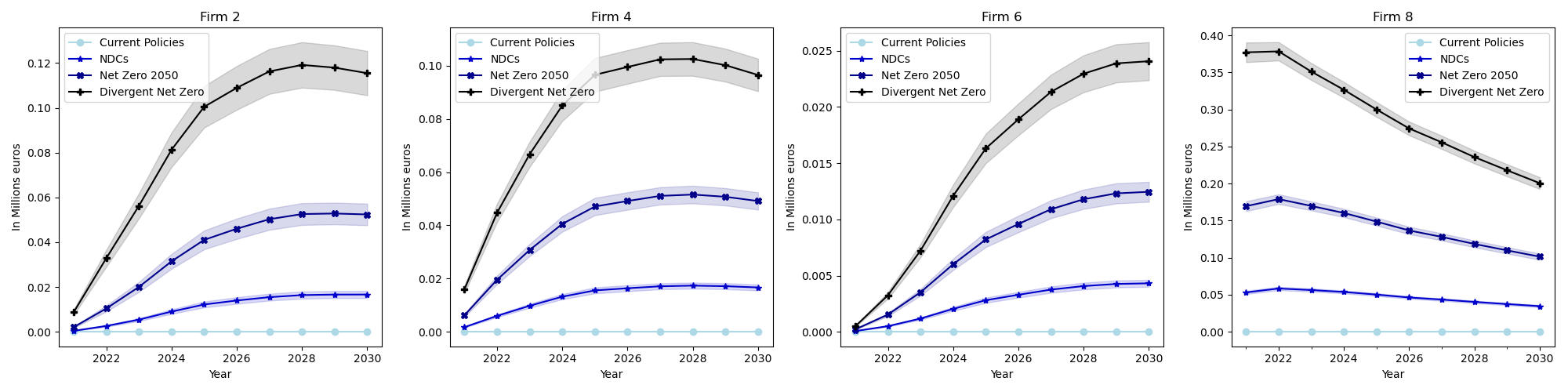
Figure 13: Average annual EL per scenario for some firms

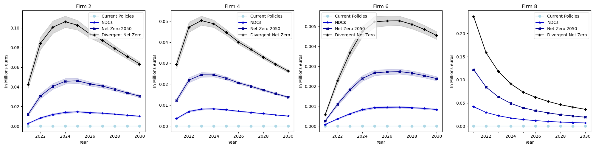
Figure 14: Average annual UL per scenario for some firms

References

- [1] T. Allen, S. Dees, V. Chouard, L. Clerc, A. de Gaye, A. Devulder, S. Diot, N. Lisack, F. Pegoraro, M. Rabate, R. Svartzman, and L. Vernet, Climate-related scenarios for financial stability assessment: an application to France, tech. rep., Banque de France, 2020. Banque de France Working Paper.
- [2] D. Baker, J. B. De Long, and P. R. Krugman, Asset returns and economic growth, Brookings Papers on Economic Activity, 2005 (2005), pp. 289–330.
- [3] A. Bangia, F. X. Diebold, A. Kronimus, C. Schagen, and T. Schuermann, Ratings migration and the business cycle, with application to credit portfolio stress testing, Journal of Banking & Finance, 26 (2002), pp. 445–474.
- [4] W. Bank, GDP (current US$) - France. World Bank. data.worldbank.org/indicator/NY.GDP.MKTP.CD.
- [5] D. Barrera, S. Crépey, E. Gobet, H.-D. Nguyen, and B. Saadeddine, Learning value-at-risk and expected shortfall, arXiv:2209.06476, (2022).
- [6] S. Battiston and I. Monasterolo, A climate risk assessment of sovereign bonds’ portfolio. ssrn:3376218, 2019.
- [7] V. Berinde and F. Takens, Iterative approximation of fixed points, vol. 1912, Springer, 2007.
- [8] V. Bouchet and T. Le Guenedal, Credit risk sensitivity to carbon price, Available at SSRN 3574486, (2020).
- [9] F. Bourgey, E. Gobet, and Y. Jiao, Bridging socioeconomic pathways of CO2 emission and credit risk. HAL:03458299, 2021.
- [10] F. Cartellier, Climate stress testing, an answer to the challenge of assessing climate-related risks to the financial system? SSRN:4179311, 2022.
- [11] V. Castro, Macroeconomic determinants of the credit risk in the banking system: The case of the GIPSI, Economic Modelling, 31 (2013), pp. 672–683.
- [12] A. Devulder and N. Lisack, Carbon tax in a production network: Propagation and sectoral incidence, Working Paper, (2020).
- [13] P. A. Diamond, National debt in a neoclassical growth model, The American Economic Review, 55 (1965), pp. 1126–1150.
- [14] Eurostat, Air emissions intensities by NACE Rev. 2 activity, 2023.
- [15] S. L. Fed, Federal Reserve Economic Data — FRED — St. Louis Fed, 2023.
- [16] J. Galí, Monetary policy, inflation, and the business cycle: an introduction to the new Keynesian framework and its applications, Princeton University Press, 2015.
- [17] J. Garnier, The Climate Extended Risk Model (CERM). arXiv:2103.03275, 2021.
- [18] J.-B. Gaudemet, J. Deshamps, and O. Vinciguerra, A stochastic climate model - an approach to calibrate the climate-extended risk model (CERM). Green RW, 2022.
- [19] M. Golosov, J. Hassler, P. Krusell, and A. Tsyvinski, Optimal taxes on fossil fuel in general equilibrium, Econometrica, 82 (2014), pp. 41–88.
- [20] M. B. Gordy, A risk-factor model foundation for ratings-based bank capital rules, Journal of Financial Intermediation, 12 (2003), pp. 199–232.
- [21] M. B. Gordy and E. Heitfield, Estimating default correlations from short panels of credit rating performance data, Working Paper, (2002).
- [22] M. B. Gordy and S. Juneja, Nested simulation in portfolio risk measurement, Management Science, 56 (2010), pp. 1833–1848.
- [23] J. D. Hamilton, Time series analysis, Princeton University Press, 2020.
- [24] H. A. Hammad, H. U. Rehman, and M. De la Sen, A new four-step iterative procedure for approximating fixed points with application to 2d Volterra integral equations, Mathematics, 10 (2022), p. 4257.
- [25] L. Kilian and H. Lütkepohl, Structural vector autoregressive analysis, Cambridge University Press, 2017.
- [26] L. Kruschwitz and A. Löffler, Stochastic discounted cash flow: a theory of the valuation of firms, Springer Nature, 2020.
- [27] T. Le Guenedal and P. Tankov, Corporate debt value under transition scenario uncertainty. SSRN:4152325, 2022.
- [28] G. Livieri, D. Radi, and E. Smaniotto, Pricing transition risk with a jump-diffusion credit risk model: Evidences from the cds market. arXiv:2303.12483, 2023.
- [29] G. Luderer, M. Leimbach, N. Bauer, E. Kriegler, L. Baumstark, C. Bertram, A. Giannousakis, et al., Description of the REMIND model (v. 1.6). SSRN:2697070, 2015.
- [30] J. Miranda-Pinto and E. R. Young, Comparing dynamic multisector models, Economics Letters, 181 (2019), pp. 28–32.
- [31] NGFS, NGFS Scenarios Portal. NGFS Scenarios Portal.
- [32] P. Nickell, W. Perraudin, and S. Varotto, Stability of rating transitions, Journal of Banking & Finance, 24 (2000), pp. 203–227.
- [33] B. C. on Banking Supervision, Basel III: Finalising Post-crisis Reforms, 12 2017. Committee on Banking Supervision (BCBS). https://www.bis.org/bcbs/publ/d424_hlsummary.pdf.
- [34] M. H. Pesaran, T. Schuermann, B.-J. Treutler, and S. M. Weiner, Macroeconomic dynamics and credit risk: a global perspective, Journal of Money, Credit and Banking, (2006), pp. 1211–1261.
- [35] P. Reis and M. Augusto, The terminal value (tv) performing in firm valuation: The gap of literature and research agenda, Journal of Modern Accounting and Auditing, 9 (2013), pp. 1622–1636.
- [36] D. Romer, Advanced Macroeconomics, 4th Edition, New York: McGraw-Hill, 2012.
- [37] T. Roncalli, Handbook of Financial Risk Management, Chapman & Hall/CRC Financial Mathematics Series, 2020.
- [38] R. M. Solow, A contribution to the theory of economic growth, The Quarterly Journal of Economics, 70 (1956), pp. 65–94.
- [39] A. Yeh, J. Twaddle, M. Frith, et al., Basel II: A new capital framework, Reserve Bank of New Zealand Bulletin, 68 (2005), pp. 4–15.