TransFusion: Generating Long, High Fidelity Time Series using Diffusion Models with Transformers

Abstract

The generation of high-quality, long-sequenced time-series data is essential due to its wide range of applications. In the past, standalone Recurrent and Convolutional Neural Network-based Generative Adversarial Networks (GAN) were used to synthesize time-series data. However, they are inadequate for generating long sequences of time-series data due to limitations in the architecture. Furthermore, GANs are well known for their training instability and mode collapse problem. To address this, we propose TransFusion, a diffusion, and transformers-based generative model to generate high-quality long-sequence time-series data. We have stretched the sequence length to 384, and generated high-quality synthetic data. To the best of our knowledge, this is the first study that has been done with this long-sequence length. Also, we introduce two evaluation metrics to evaluate the quality of the synthetic data as well as its predictive characteristics. We evaluate TransFusion with a wide variety of visual and empirical metrics, and TransFusion outperforms the previous state-of-the-art by a significant margin.

1 Introduction

Synthetic time-series generation has been a popular research field in recent years due to its wide variety of applications. Electronic health record (EHR) generation, trajectory generation, and vehicle routing need tremendous amounts of data to learn the pattern in the samples. Unfortunately, it is challenging to get a hold of real data due to the lack of public access to the dataset [1]. Synthetic data can be a solution to mitigate this problem [2, 3]. However, generating synthetic time-series data is challenging due to its random nature. In recent years, researchers used different generative techniques like Variational Auto Encoders (VAE) and Generative Adversarial Networks (GAN) to generate synthetic time series data [4, 5, 6, 7, 8]. But these studies were done using shorter sequence lengths (less than 100). Also, training GAN is extremely unstable, and it is prone to the mode-collapse problem [9], where the model provide limited sample variety. Generating long-sequenced time-series data is necessary to understand the data context better. The longer the sequence length is, the more information it can capture about the data over time. For example, monitoring a diabetic patient’s blood sugar level for a long time will reveal patterns and trends better than monitoring for a short period of time.

Capturing temporal dependencies in long-sequential data is challenging for standalone Convolutional Neural Networks (CNN) and Recurrent Neural Networks (RNN) because of their architectural limitations [10, 11]. Most of the evaluation metrics for synthetic time series are also CNN and RNN based. So, new metrics are needed for evaluating synthetic time series with long sequences.

Diffusion-based models have garnered extensive interest for their potential in the Computer Vision (CV) and Natural Language Processing (NLP) domains [12, 13, 14]. These models gradually add noise to the input data and make it a noisy data distribution. Adding noise to the data is called the forward diffusion process. And then, a neural network architecture tries to remove the noise and learn the data distribution of the real data. This process is called the backward diffusion process. After training, the diffusion-based generative model can generate high-quality synthetic data. On top of this, these models overcome the mode-collapse problem by learning the semantic nature of the data. Though much interesting work has been done in the CV and NLP domain using diffusion models, time-series generation is still unexplored.

In this study, we present TransFusion, a diffusion-based model to generate high-quality time series data. We use a transformers encoder [15] in the backward diffusion process to approximate the real data distribution. As the transformer encoder consists of the attention mechanism, it can capture the long-term temporal dependencies. We conduct extensive experiments with the data consisting of sequences of length 100. We further investigate the generated data quality by TransFusion on the sequence length 384. We perform various evaluations using visual (PCA & t-SNE) and empirical metrics. Since existing evaluation metrics for synthetic data are based on RNN and CNN architectures, they are unable to capture long-term dependencies. Therefore, we propose two transformers-based evaluation metrics to distinguish between synthetic and original data (post-hoc classifier) and to see if the synthetic data preserves the predictive characteristics of the original data by using a sequence prediction task, respectively. We find that, TransFusion outperforms other state-of-the-art methods in these evaluations in generating long-sequence time-series data.

Our contribution to this work is as follows:

• We introduce TransFusion, a diffusion-based generative model, capable of generating long-sequence, high-fidelity time series data that outperforms previous state-of-the-art time series generative models, such as GT-GAN [8], TimeGAN [4], CotGAN [7], etc.

• We propose two evaluation metrics for synthetic time series data which can distinguish original and synthetic data and provide an overview of the synthetic data’s performance over sequence prediction tasks.

• We show the quality of the generated data using a wide variety of evaluation metrics (both visual and empirical).

• By conducting an ablation study, we show the combination of diffusion model and transformers is needed for generating high-quality, long-sequenced time series data.

2 Related Works

Time-series generation has seen an increased amount of interest in recent years for its applications. In most research, Generative Adversarial Networks (GAN) have been used to generate synthetic time series data. GAN has been widely used in computer vision (CV) and Natural Language Processing (NLP) domains with a high success rate [16, 17]. For the time series generation, most of the studies used Recurrent Neural Network (RNN) and Convolutional Neural Network (CNN) based architecture. For example, C-RNN-GAN [5] used Recurrent Neural Network based GAN to generate music. TimeGAN [4], used a combination of supervised and unsupervised learning to generate time series data, and in the architecture, they also used Recurrent Neural Networks. A Convolutional Neural Network based architecture was used in Energy Based GAN [18], where the author used this CNN architecture in the discriminator, which was later used as an Autoencoder. Causal optimal transport was used to generate the time sequence in CotGAN [7]. WaveGAN [19] uses combination of Transposed Convolutional Neural Networks in its generator for generating audio data and QuantGAN [20] uses Temporal Convolutional Networks (TCN) [21] to generate financial time-series data. GT-GAN [8] used a combination of GANs, Autoencoders, Neural Ordinary Differential Equations [22], Neural Controlled Differential Equations [23], and Continuous time-flow processes [24] for time series generation. Although standalone RNN and CNN architectures have been used widely, these architectures are not well suited for generating longer sequences, because they cannot capture the long-term time dependencies. So, all of the studies mentioned above cannot generate meaningful time series data when the sequence length is longer such as a sequence length of more than 100 (we show in Table 1). Besides these issues, training GAN is extremely difficult and it is prone to the mode collapse problem.

In contrast, the diffusion-based model has recently caught the attention of researchers and it is yielding promising results in both the CV and NLP domains. Diffusion-based generative models with the correct architecture are capable of generating high quality samples. Also these models are not limited to the mode collapse problem which provides an advantage over the GAN-based models. Generation of time-series using a diffusion-based architecture is fairly new. It has been tested on conditional and unconditional video generation [25] tasks, and audio generation tasks [26]. In Diffwave [26], the author used a Convolutional Neural Network-based diffusion model that can synthesize audio and outperforms previous GAN-based audio synthesis work. In another audio generation task, the author tried to combine diffusion-based models and GAN-based models for Mandarin-based voice synthesis [27]. It is important to note that most audio data is low dimensional in nature. This is in contrast to general time-series data, which can often be high-dimensional.

In this study, we leverage the use of transformers architecture to capture the long-term dependencies of time and combine it with the diffusion model. Also, to distinguish original data from synthetic data for long-sequences, we propose a transformer-based post-hoc classifier. Additionally, to see the predictive characteristics in the synthetic data, we also propose a metric called long-sequence predictive score (LPS).

3 Preliminaries

In this section, we formulate the problem definition and give some background information to accompany the paper.

3.1 Problem Statement

Given a time series data $x\sim q(x)\in\mathbb{R}^{D}$, where $x=\{x^{1},x^{2},x^{3},...,x^{N}\}$, $N$ is the sequence length of time series data, and $D$ is the data dimension, we need to train a generative model that will learn $p_{\theta}(x)$ which approximate $q(x)$ best.

In this study, we use diffusion-based models as generative models to synthesize time-series data.

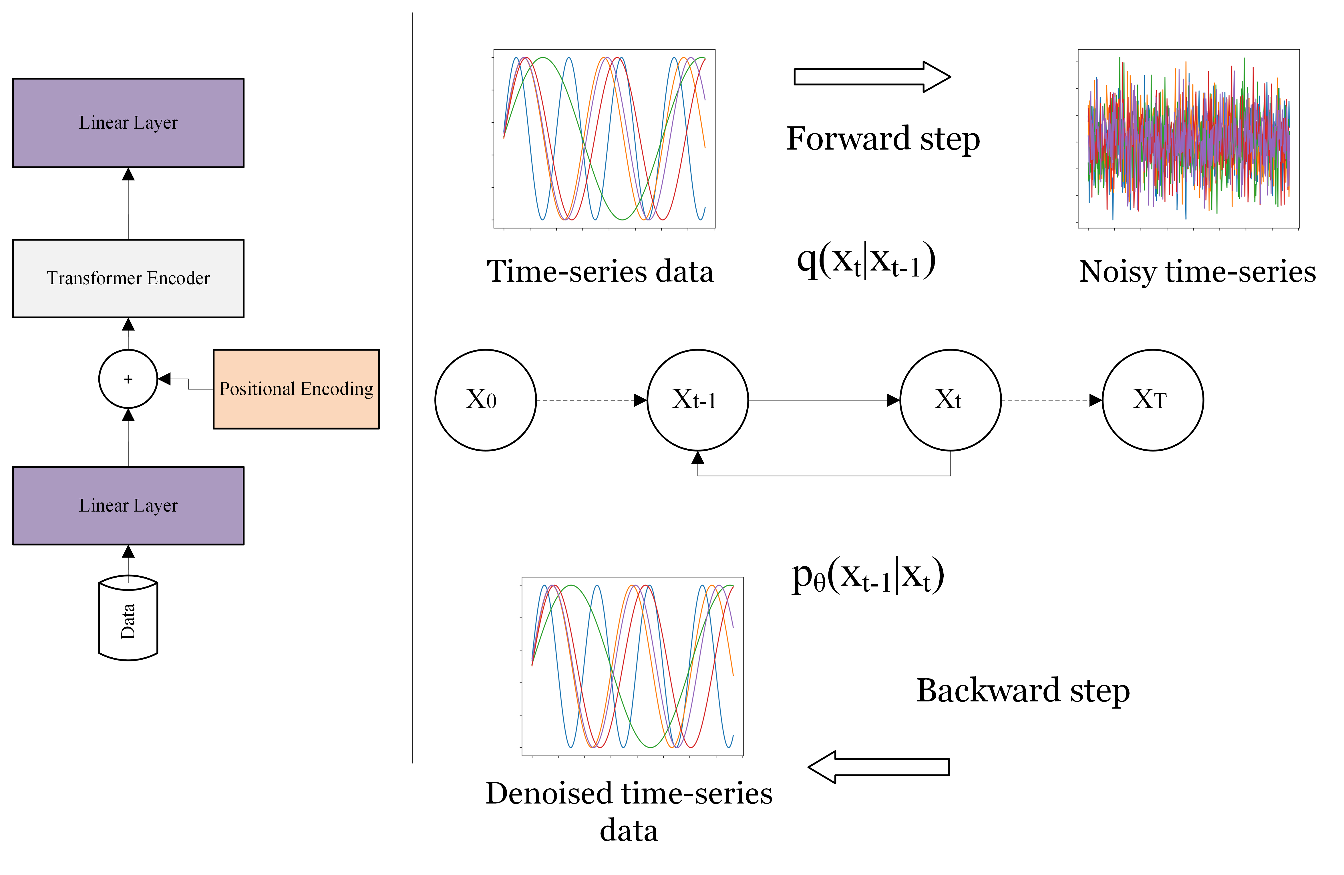
Figure 1: TransFusion Architecture, Transformers block that used in the TransFusion (left part), working process of diffusion (right part)

3.2 Denoising Diffusion Probabilistic Model (DDPM)

The denoising diffusion probabilistic model [12] works in two steps. First, it takes data $x_{0}\sim q(x_{0})$ and over the time it adds Gaussian noise and after $T$ steps, the data should become pure Gaussian noise $x_{T}$ (if $T$ is higher [13]). How much noise is added to each step is calculated by the variance schedule $\beta_{t}$. So the forward diffusion process can be defined as follows:

$$q(x_{1:T}|x_{0})=\prod_{t=1}^{T}q(x_{t}|x_{t-1})$$ (1)

$$q(x_{t}|x_{t-1})=\mathcal{N}(x_{t};\sqrt{1-\beta_{t}}x_{t-1},\beta_{t}\textbf{I})$$ (2)

After further calculation, it is possible to sample $x_{t}$ at any given time given $x_{0}$ as they are Gaussian.

$$q(x_{t}|x_{0})=\mathcal{N}(x_{t};\sqrt{\bar{\alpha_{t}}}x_{0},(1-\bar{\alpha_{t}})\textbf{I})$$ (3)

Here, $\alpha_{t}=1-\beta_{t}$ and $\bar{\alpha_{t}}=\prod_{s=0}^{t}\alpha_{s}$. In the backward diffusion process, a model is trained to learn $p_{\theta}$ that approximate $q(x_{t-1}|x_{t})$ because it is not possible to learn $q(x_{t-1}|x_{t})$ directly as it needs the knowledge of the whole data distribution.

$$p_{\theta}(x_{t-1}|x_{t})=\mathcal{N}(x_{t-1},\mu_{\theta}(x_{t},t),\Sigma_{\theta}(x_{t},t))$$ (4)

In practice, a neural network is used to learn the distribution $p_{\theta}(x_{t-1}|x_{t})$, and it tries to predict the parameters $\mu_{\theta}(x_{t},t)$ and $\Sigma_{\theta}(x_{t},t)$. DDPM [12] achieved the best result with a fixed variance $\sigma^{2}\textbf{I}$. And the mean $\mu_{\theta}(x_{t},t)$ is calculated as follows:

$$\mu_{\theta}(x_{t},t)=\frac{1}{\sqrt{\alpha_{t}}}\big{(}x_{t}-\frac{\beta_{t}}{\sqrt{1-\bar{\alpha_{t}}}}\epsilon_{\theta}(x_{t},t)\big{)}$$ (5)

So we can re-write equation 4 as:

$$\begin{split}p_{\theta}(x_{t-1}|x_{t})=\mathcal{N}(x_{t-1},\frac{1}{\sqrt{\alpha_{t}}}\big{(}x_{t}-\frac{\beta_{t}}{\sqrt{1-\bar{\alpha_{t}}}}&\epsilon_{\theta}(x_{t},t)\big{)},\\ &\sigma^{2}\textbf{I})\end{split}$$ (6)

Also the training objective defined by DDPM is,

$$L_{simple}=\mathbb{E}_{t,x_{0},\epsilon}\big{[}||\epsilon-\epsilon_{\theta}(x_{t},t)||^{2}\big{]}$$ (7)

where, $\epsilon\sim\mathcal{N}(0,\textbf{I})$

4 TransFusion: Transformers Diffusion Model

In this study, we introduce a diffusion model-based time-series generative model called TransFusion. We use the transformer encoder as the neural network architecture to approximate the target data distribution for the backward diffusion process. Figure 1 shows the overall architecture of the TransFusion.

For the forward diffusion process, we use the cosine variance scheduler [12] to calculate the amount of noise added in each time-step. In the neural network architecture, the time-series data goes through a linear layer, positional encoding, then to the transformer encoder. Positional encoding is used to keep track of the data in each time-step. Then the data is passed through another linear layer to make it the same shape as the original data.

Over time the network tries to denoise the data and learn to approximate the original data distribution using the objective equation 7. Algorithm 1 [12] and 2 show how TransFusion is trained and how samples are generated from it.

Algorithm 1 Training

Input: Pre-calculated variance schedule $\beta$

repeat

     sample $x_{0}\sim q(x_{0})$, $\epsilon\sim\mathcal{N}(0,\textbf{I})$, $t\sim\mathcal{U}(\{1,..,T\})$

     Take Gradient step on

     $\nabla_{\theta}||\epsilon-\epsilon_{\theta}(x_{t},t)||^{2}$

until converged

Algorithm 2 Sampling

sample $x_{T}\sim\mathcal{N}(0,\textbf{I})$

for $t=T,...,1$ do

     sample $x_{t-1}\sim p_{\theta}(x_{t-1|x_{t}})$ using equation 6

end for

return: $x_{0}$

5 Experimental Results

We perform extensive experiments with four time-series datasets and compare the results with seven time-series generative models, TimeGAN [4], C-RNN-GAN [5], EBGAN [18], CotGAN [7], WaveGAN [19], QuantGAN [20], and GT-GAN [8]. We use sequence lengths $100$ and $384$ for the experiments. The result shows that even at this high sequence length (384), TransFusion is capable of generating high-quality synthetic data. We evaluate our study with various evaluation metrics, including qualitative and quantitative analysis. We also propose two evaluation metrics to assess the predictive nature of the synthetic data and to evaluate if the original data and the synthetic data are distinguishable. We also present an ablation analysis to show that the combination of diffusion and transformers is necessary to generate long-sequenced time-series data. Datasets preprocessing procedure, hyperparameters of the TransFusion and benchmarking models can be found in the appendices A, B.

5.1 Datasets

We use four time-series datasets for this experiment (one simulated and three real-world datasets).

5.1.1 Sine Data

We create a sinusoidal function $f(x)$ that generates sine wave data with a dimension of five with various frequencies and phases. The function generates $x_{i}(t)=sin(2\pi ft+\phi)$, here $f$ represents the frequency and it is sampled from a uniform distribution, $f\sim\mathcal{U}[0,1]$, the phase $\phi$ is as well sampled from the uniform distributions, $\phi\sim\mathcal{U}[-\pi,\pi]$. The phase is different in each dimension $i\in{1,2,...,5}$.

5.1.2 Stock

We use Google stock data for the time between 2004 to 2017. This dataset contains six stock features (opening, closing, highest, lowest, and adjacent closing values) per day.

5.1.3 Energy Consumption

We also test our model using high-dimensional, noisy energy consumption data from the UCI repository [28]. This dataset contains the electricity consumption of households at 10 minutes intervals for 4.5 months. It has 28 features, including electricity consumption in kilowatts per hour, temperature, humidity reading in various rooms, wind speed, pressure, etc.

5.1.4 Air Quality

Finally, we consider using another high-dimensional dataset on air quality [29] from the UCI repository. This dataset was collected from an Italian city hourly and recorded for one year. The data contains 13 features, including the level of carbon mono-oxide (CO), benzin level, etc. in the air.

5.2 Evaluation Metrics

We evaluate the quality of the synthetic data in terms of fidelity (does the generated data comes from the same distributions as the original one), diversity (is the generated data diverse enough to fit the whole data) and check if the generative model is demonstrating the mode-collapse problem or not. We also implement a transformers-based post-hoc classifier metric, Long-Sequence Discriminative Score (LDS) that evaluates the fidelity of the synthetic data. Additionally, we implement a transformers-based sequence prediction metric, Long-Sequence Predictive Score (LPS) to observe the predictive characteristics in the synthetic data. In order to evaluate the predictive characteristics of the synthetic data beyond LPS, we conduct another sequence prediction task. The goal of the task is to predict the next five steps of feature vectors given an input sequence.

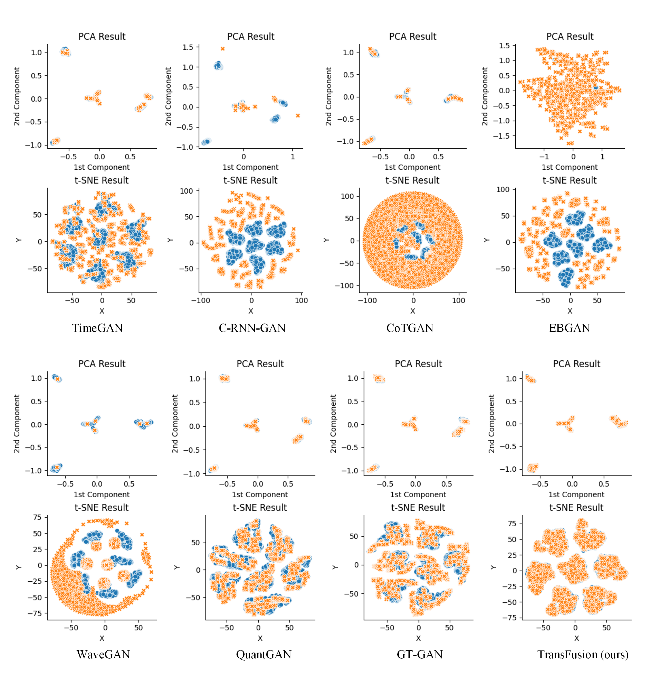
Figure 2: PCA and t-SNE plots of TimeGAN, C-RNN-GAN, CoTGAN, EBGAN, WaveGAN, QuantGAN, GT-GAN, and TransFusion (ours) on the Energy Dataset (dimension = 28), Sequence length: 100. Each dot represents a sequence of time series data, blue and orange represents real and synthetic data respectively, if the generative model learns to approximate the real data distributions, the blue and orange dots should overlap

5.2.1 PCA & t-SNE plots

To evaluate the quality of the synthetic data, we use both Principal Component Analysis [30], and t-distributed Stochastic Neighbor Embedding [31] techniques. They show how closely the distribution of synthetic data resembles real data in 2-dimensional space and also show if the generated data covers the area of the original data. This gives us the fidelity and diversity evaluation of the synthetic data.

5.2.2 Long-Sequence Discriminative Score

We create an evaluation metric to determine if the synthetic data is indistinguishable from the original data. In order to use this metric, first we train a transformers-based [15] (only using a transformers encoder) post-hoc classifiers with the original & synthetic data labeled as original and fake, respectively. Then we use the held-out dataset to measure the classification error. This metric is inspired by the discriminative score from the TimeGAN [4]. But the discriminative score from TimeGAN uses a RNN-based classifier, which may not work when the sequence length is long. Consequently, we use a transformer-based classifier to capture long-term time dependencies. This metric provides an evaluation of the fidelity of the assessment.

5.2.3 Long-Sequence Predictive Score

To check if the synthetic data captured the predictive characteristics of the original data or not, we create a transformers-based sequence prediction task called long-sequence predictive score (LPS). Here we train a transformers-based sequence prediction model to predict the next step feature vector given an input sequence. The metric was also inspired by TimeGAN’s predictive score [4], but since TimeGAN’s predictive score uses a RNN-based model, it may not be suitable for long-sequenced tasks. We train the model using synthetic data and then evaluate it using the original dataset. The mean absolute error (MAE) is used to measure the performance of the LPS. In addition, we extend the LPS to predict the next five steps (+5 Steps Ahead) feature vectors given the input sequence to see how features evolve over time.

5.2.4 Jensen-Shannon Divergence

This quantitative evaluation metric measures if the original and the synthetic data come from the same distributions or not. A lower JSD [32] score means the distributions are similar between the original and synthetic datasets.

5.2.5 $\alpha$-precision, $\beta$-recall & Coverage

$\alpha$-precision and $\beta$-recall [33] also provide the assessment of fidelity and diversity, respectively, of the synthetic data. And coverage [34] checks the mode-dropping issue in the generative models by using nearest neighbor manifolds [35] and measuring the fraction of the original samples whose neighborhoods contain at least one synthetic sample.

5.3 Visualization Results

For the qualitative comparison, we use the PCA and t-SNE plots of our generative models and compare them with other model plots. Figure 2, shows the plots of the energy dataset, sequence length 100 (high-dimensional data in our experiment). Each dot in the plot represents a sequence of data. We can observe, for TransFusion, the generated data’s dot is closer to the original data. This indicates that our generative model learns the distribution of the original data and is capable of generating high-quality data.

Table 1: Resutls on Different Time-Series Datasets, Sequence Length: 100, we report the mean and standard deviation (bold indicates best result, $\uparrow$ indicates higher as better, $\downarrow$ indicates lower as better)

	Evaluation Metrics
Dataset	Model Name	LDS	LPS	JSD	$\alpha$-	$\beta$-	Coverage	+ 5 Steps
					precision	recall		Ahead
		($\downarrow$)	($\downarrow$)	($\downarrow$)	($\uparrow$)	($\uparrow$)	($\uparrow$)	($\downarrow$)
	TimeGAN	0.499 $\pm$ .001	0.253 $\pm$ .001	0.11 $\pm$ .00	0.863 $\pm$ .00	0.089 $\pm$ .00	0.355 $\pm$ .00	0.257 $\pm$ .005
	CotGAN	0.467 $\pm$ .003	0.249 $\pm$ .001	0.10 $\pm$ .00	0.795 $\pm$ .00	0.984 $\pm$ .00	0.852 $\pm$ .00	0.253 $\pm$ .001
	C-RNN-GAN	0.5 $\pm$ .00	0.649 $\pm$ .001	0.53 $\pm$ .00	0.00 $\pm$ .00	0.00 $\pm$ .00	0.00 $\pm$ .00	0.651 $\pm$ .001
Sine	EBGAN	0.499 $\pm$ .001	0.260 $\pm$ .001	0.32 $\pm$ .00	0.901 $\pm$ .00	0.00 $\pm$ .00	0.322 $\pm$ .00	0.261 $\pm$ .001
	WaveGAN	0.500 $\pm$ .000	0.353 $\pm$ .001	0.414 $\pm$ .00	0.00 $\pm$ .00	0.00 $\pm$ .00	0.000 $\pm$ .00	0.351 $\pm$ .001
	QuantGAN	0.469 $\pm$ .013	0.249 $\pm$ .001	0.253 $\pm$ .00	0.992 $\pm$ .00	0.384 $\pm$ .00	0.823 $\pm$ .00	0.253 $\pm$ .001
	GT-GAN	0.465 $\pm$ .001	0.246 $\pm$ .001	0.048 $\pm$ .00	0.684 $\pm$ .00	0.954 $\pm$ .00	0.737 $\pm$ .00	0.253 $\pm$ .001
	TransFusion (ours)	0.097 $\pm$ .042	0.243 $\pm$ .001	0.02 $\pm$ .00	0.992 $\pm$ .00	0.974 $\pm$ .00	0.963 $\pm$ .00	0.245 $\pm$ .001
	TimeGAN	0.494 $\pm$ .001	0.062 $\pm$ .001	0.11 $\pm$ .00	0.994 $\pm$ .00	0.649 $\pm$ .00	0.073 $\pm$ .00	0.063 $\pm$ .001
	CotGAN	0.494 $\pm$ .001	0.066 $\pm$ .001	0.010 $\pm$ .00	0.827 $\pm$ .00	0.837 $\pm$ .00	0.295 $\pm$ .00	0.067 $\pm$ .001
	C-RNN-GAN	0.19 $\pm$ .03	0.068 $\pm$ .001	0.05 $\pm$ .00	0.899 $\pm$ .00	0.963 $\pm$ .00	0.605 $\pm$ .00	0.069 $\pm$ .001
Stock	EBGAN	0.5 $\pm$ .00	0.495 $\pm$ .001	0.66 $\pm$ .00	0.487 $\pm$ .00	0.00 $\pm$ .00	0.011 $\pm$ .00	0.496 $\pm$ .001
	WaveGAN	0.496 $\pm$ .007	0.064 $\pm$ .000	0.272 $\pm$ .00	1.000 $\pm$ .00	0.000 $\pm$ .00	0.010 $\pm$ .00	0.064 $\pm$ .001
	QuantGAN	0.497 $\pm$ .003	0.062 $\pm$ .000	0.824 $\pm$ .00	0.660 $\pm$ .00	0.826 $\pm$ .00	0.405 $\pm$ .00	0.063 $\pm$ .001
	GT-GAN	0.416 $\pm$ .026	0.071 $\pm$ .001	0.048 $\pm$ .00	0.684 $\pm$ .00	0.954 $\pm$ .00	0.737 $\pm$ .00	0.071$\pm$ .001
	TransFusion (ours)	0.498 $\pm$ .001	0.060$\pm$ .001	0.018 $\pm$ .00	0.97 $\pm$ .00	0.99 $\pm$ .00	0.93 $\pm$ .00	0.061 $\pm$ .001
	TimeGAN	0.497 $\pm$ .001	0.002 $\pm$ .001	0.11 $\pm$ .00	0.916 $\pm$ .00	0.343 $\pm$ .00	0.278 $\pm$ .00	0.003 $\pm$ .001
	CotGAN	0.482 $\pm$ .017	0.006 $\pm$ .001	0.10 $\pm$ .00	0.850 $\pm$ .00	0.617 $\pm$ .00	0.687 $\pm$ .00	0.006 $\pm$ .001
	C-RNN-GAN	0.5 $\pm$ 0.00	0.061 $\pm$ .001	0.344 $\pm$ .00	1.00 $\pm$ .00	0.00 $\pm$ .00	0.001 $\pm$ .00	0.065 $\pm$ .001
Air	EBGAN	0.5 $\pm$ .00	0.872 $\pm$ .106	0.423 $\pm$ .00	0.00 $\pm$ .00	0.00 $\pm$ .001	0.00 $\pm$ .00	0.813 $\pm$ .001
	WaveGAN	0.439 $\pm$ .034	0.009 $\pm$ .001	0.595 $\pm$ .00	0.942 $\pm$ .00	0.586 $\pm$ .00	0.750 $\pm$ .00	0.010 $\pm$ .001
	QuantGAN	0.464 $\pm$ .030	0.002 $\pm$ .001	0.555 $\pm$ .00	0.983 $\pm$ .00	0.506 $\pm$ .00	0.749 $\pm$ .00	0.002 $\pm$ .001
	GT-GAN	0.491 $\pm$ .005	0.003 $\pm$ .001	0.065 $\pm$ .00	0.687 $\pm$ .00	0.938 $\pm$ .00	0.824 $\pm$ .00	0.003 $\pm$ .001
	TransFusion (ours)	0.148 $\pm$ .029	0.001 $\pm$ .001	0.027 $\pm$ .00	0.926 $\pm$ .00	0.956 $\pm$ .00	0.944 $\pm$ .00	0.002 $\pm$ .001
	TimeGAN	0.490 $\pm$ .001	0.015 $\pm$ .001	0.176 $\pm$ .00	0.816 $\pm$ .00	0.213 $\pm$ .00	0.076 $\pm$ .00	0.015 $\pm$ .001
	CotGAN	0.497 $\pm$ .002	0.066 $\pm$ .001	0.183 $\pm$ .00	0.968 $\pm$ .00	0.374 $\pm$ .00	0.28 $\pm$ .00	0.067 $\pm$ .001
	C-RNN-GAN	0.5 $\pm$ .00	0.264 $\pm$ .001	0.170 $\pm$ .34	0.00 $\pm$ .00	0.00 $\pm$ .00	0.00 $\pm$ .00	0.215 $\pm$ .001
Energy	EBGAN	0.5 $\pm$ 0.00	0.971 $\pm$ .001	0.49 $\pm$ .00	0.00 $\pm$ .00	0.00 $\pm$ .00	0.00 $\pm$ .00	0.971 $\pm$ .001
	WaveGAN	0.496 $\pm$ .010	0.012 $\pm$ .000	0.211 $\pm$ .00	1.000 $\pm$ .00	0.00 $\pm$ .00	0.014 $\pm$ .00	0.012 $\pm$ .001
	QuantGAN	0.498 $\pm$ .002	0.012 $\pm$ .000	0.826 $\pm$ .00	0.793 $\pm$ .00	0.701 $\pm$ .00	0.373 $\pm$ .00	0.012 $\pm$ .001
	GT-GAN	0.423 $\pm$ .030	0.012 $\pm$ .001	0.158 $\pm$ .00	0.820 $\pm$ .00	0.26 $\pm$ .00	0.391 $\pm$ .00	0.012 $\pm$ .001
	TransFusion (ours)	0.332 $\pm$ .019	0.011 $\pm$ .001	0.016 $\pm$ .00	0.983 $\pm$ .00	0.876 $\pm$ .00	0.847 $\pm$ .00	0.012$\pm$ .001

Table 2: Resutls on Different Time-Series Datasets, Sequence Length: 384, we report the mean and standard deviation (bold indicates best result, $\uparrow$ indicates higher as better, $\downarrow$ indicates lower as better)

	Evaluation Metrics
Dataset	Model Name	LDS	LPS	JSD	$\alpha$-	$\beta$-	Coverage	+ 5 Steps
					precision	recall		Ahead
		($\downarrow$)	($\downarrow$)	($\downarrow$)	($\uparrow$)	($\uparrow$)	($\uparrow$)	($\downarrow$)
	GT-GAN	0.497 $\pm$ .003	0.313 $\pm$ .001	0.189 $\pm$ .00	0.978 $\pm$ .00	0.016 $\pm$ .00	0.162 $\pm$ .00	0.316 $\pm$ .001
Sine	CotGAN	0.370 $\pm$ .075	0.307 $\pm$ .000	0.465 $\pm$ .00	0.904 $\pm$ .00	0.984 $\pm$ .00	0.926 $\pm$ .00	0.310 $\pm$ .001
	TransFusion (ours)	0.075 $\pm$ .032	0.306 $\pm$ .001	0.006 $\pm$ .00	0.99 $\pm$ .00	0.99 $\pm$ .00	0.96 $\pm$ .00	0.301 $\pm$ .001
	GT-GAN	0.441 $\pm$ .022	0.112 $\pm$ .000	0.091 $\pm$ .00	0.961 $\pm$ .00	0.913 $\pm$ .00	0.556 $\pm$ .00	0.112 $\pm$ .001
Stock	CotGAN	0.445 $\pm$ .148	0.087 $\pm$ .000	0.804 $\pm$ .00	0.840 $\pm$ .00	0.972 $\pm$ .00	0.870 $\pm$ .00	0.087 $\pm$ .001
	TransFusion (ours)	0.483 $\pm$ .001	0.060$\pm$ .001	0.018 $\pm$ .00	0.984 $\pm$ .00	0.991 $\pm$ .00	0.984 $\pm$ .00	0.061 $\pm$ .001
	GT-GAN	0.495 $\pm$ .004	0.002 $\pm$ .000	0.182 $\pm$ .00	1.000 $\pm$ .00	0.888 $\pm$ .00	0.190 $\pm$ .00	0.003 $\pm$ .001
Air	CotGAN	0.481 $\pm$ .030	0.006 $\pm$ .000	0.780 $\pm$ .00	0.980 $\pm$ .00	0.304 $\pm$ .00	0.920 $\pm$ .00	0.005 $\pm$ .001
	TransFusion (ours)	0.162 $\pm$ .029	0.001 $\pm$ .001	0.027 $\pm$ .00	0.951 $\pm$ .00	0.956 $\pm$ .00	0.944 $\pm$ .00	0.002 $\pm$ .001
	GT-GAN	0.434 $\pm$ .041	0.012 $\pm$ .000	0.074 $\pm$ .00	0.586 $\pm$ .00	0.334 $\pm$ .00	0.480 $\pm$ .00	0.012 $\pm$ .001
Energy	CotGAN	0.472 $\pm$ .024	0.012 $\pm$ .000	0.529 $\pm$ .00	1.000 $\pm$ .00	0.000 $\pm$ .00	0.096 $\pm$ .00	0.012 $\pm$ .001
	TransFusion (ours)	0.400 $\pm$ .019	0.011 $\pm$ .001	0.012 $\pm$ .00	0.998 $\pm$ .00	0.644 $\pm$ .00	0.850 $\pm$ .00	0.011$\pm$ .001

Table 3: Ablation Study: Sequence Length: 100, we report the mean and standard deviation (bold indicates best result, $\uparrow$ indicates higher as better, $\downarrow$ indicates lower as better)

	Evaluation Metrics
Dataset	Model Name	LDS	LPS	JSD	$\alpha$-	$\beta$-	Coverage	+ 5 Steps
					precision	recall		Ahead
		($\downarrow$)	($\downarrow$)	($\downarrow$)	($\uparrow$)	($\uparrow$)	($\uparrow$)	($\downarrow$)
	TransGAN	0.500 $\pm$ .000	0.352 $\pm$ .000	0.392 $\pm$ .00	0.000 $\pm$ .00	0.000 $\pm$ .00	0.000 $\pm$ .00	0.349 $\pm$ .001
Sine	Diffusion-GRU	0.498 $\pm$ .002	0.252 $\pm$ .000	0.106 $\pm$ .00	0.946 $\pm$ .00	0.408 $\pm$ .00	0.703 $\pm$ .00	0.260 $\pm$ .001
	TransFusion (ours)	0.097 $\pm$ .042	0.243 $\pm$ .001	0.02 $\pm$ .00	0.992 $\pm$ .00	0.974 $\pm$ .00	0.963 $\pm$ .00	0.245 $\pm$ .001
	TransGAN	0.500 $\pm$ .000	0.905 $\pm$ .011	0.630 $\pm$ .00	0.000 $\pm$ .00	0.000 $\pm$ .00	0.000 $\pm$ .00	0.862 $\pm$ .001
Stock	Diffusion-GRU	0.500 $\pm$ .000	0.066 $\pm$ .000	0.273 $\pm$ .00	0.315 $\pm$ .00	0.744 $\pm$ .00	0.166 $\pm$ .00	0.067 $\pm$ .001
	TransFusion (ours)	0.498 $\pm$ .001	0.060$\pm$ .001	0.018 $\pm$ .00	0.97 $\pm$ .00	0.99 $\pm$ .00	0.93 $\pm$ .00	0.061 $\pm$ .001
	TransGAN	0.500 $\pm$ .000	0.065 $\pm$ .001	0.532 $\pm$ .00	0.000 $\pm$ .00	0.000 $\pm$ .00	0.000 $\pm$ .00	0.080 $\pm$.001
Air	Diffusion-GRU	0.500 $\pm$ .000	0.051 $\pm$ .005	0.230 $\pm$ .00	0.001 $\pm$ .00	0.049 $\pm$ .00	0.001 $\pm$ .00	0.057 $\pm$ .001
	TransFusion (ours)	0.148 $\pm$ .029	0.001 $\pm$ .001	0.027 $\pm$ .00	0.926 $\pm$ .00	0.956 $\pm$ .00	0.944 $\pm$ .00	0.002 $\pm$ .001
	TransGAN	0.500 $\pm$ .000	0.971 $\pm$ .000	0.692 $\pm$ .00	0.000 $\pm$ .00	0.000 $\pm$ .00	0.000 $\pm$ .00	0.970 $\pm$ .001
Energy	Diffusion-GRU	0.500 $\pm$ .000	0.097 $\pm$ .007	0.421 $\pm$ .00	0.000 $\pm$ .00	0.000 $\pm$ .00	0.000 $\pm$ .00	0.092 $\pm$ .001
	TransFusion (ours)	0.332 $\pm$ .019	0.011 $\pm$ .001	0.016 $\pm$ .00	0.983 $\pm$ .00	0.876 $\pm$ .00	0.847 $\pm$ .00	0.012$\pm$ .001

5.4 Empirical Evaluation

An ideal generative model should generate samples that are statistically close to the original data (fidelity) and diverse enough to cover the whole area of the original data (diversity), and the model should not fall into mode dropping (coverage). We provide multiple assessments of fidelity (LDS, JSD, $\alpha$-precision, PCA plots, t-SNE plots) and diversity ($\beta$-recall, PCA plots, t-SNE plots) and also show if the generative models are suffering from the mode-collapse problem or not (coverage). We also show the predictive characteristicness of the synthetic data by using LPS and +5 Steps Ahead score.

In our experiments, we use both high dimensional and long-sequenced data (Air Quality, Energy Consumption). Table 1 indicates the results of our experiment for sequence length 100. We run the evaluation metrics ten times and report the mean and standard deviation in the table. Overall, TransFusion performs better than all the state-of-the-art generative models. We achieve a significantly higher score in every metric. Although some of the other methods get a high score in some metrics, if we consider all the aspects of fidelity, diversity, and coverage, we observe that TransFusion outperforms them all. The combination of diffsuion model and Transformers make it possible to generate high-dimensional and long-sequenced data. Whereas, Generative Adversarial Networks based architecture provide limited sample variety due to the mode-collapse problem, also as they use CNN, RNN-based architecture, they fail to generate long-sequenced data.

From Table 1, we can observe our evaluation metrics, LDS and LPS reflect the results with other metrics. Transfusion achieve a 22% higher score than the GT-GAN (most recent time-series generative model) on the Long-Sequence Discriminative Score for the energy dataset. Also, from the coverage metric, we see that, except TransFusion, all the models suffer mode-collapse when the data is high dimensional (energy dataset). So, these state-of-the-art methods can not keep up with the long-sequence high-dimensional data. On top of these, the synthetic data generated by TransFusion achieve the best score on both LPS and +5 steps ahead prediction tasks. Therefore, synthetic data generated by TransFusion can be used in the forecasting tasks.

Furthermore, we also stretch the sequence length of the datasets to 384 to observe the robustness of our model and compare the result with GT-GAN and CotGAN (two recent models). Table 2 shows the outcome. We see that both GT-GAN and CotGAN can not keep up with the long-sequence data, and suffer the mode-collapse problem.

Besides empirical evaluation, training time is another factor to consider. TransFusion is able to generate high-quality samples by only training for 5 hours whereas GT-GAN takes nearly 28 hours to produce their result. All the experiments were run on an NVIDIA A100 GPU with 40GB of memory.

5.5 Ablation Study

The combination of the diffusion model and transformers architecture allows us to generate long-sequenced, high-quality samples, as evidenced by the ablation study. For this, we train a transformers-based Generative Adversarial Network (TransGAN), where the transformer’s encoder serves as both generator and discriminator. We also train a diffusion model without transformers. For the diffusion model’s backward process, we use the Gated Recurrent Unit (GRU). Table 3 shows the analysis of the experiment. We use sequence length 100 for the ablation study. We can see both TransGAN and Diffusion-GRU is unable to keep up with the TransFusion.

6 Limitations and Future Work

While diffusion-based generative models are fast in terms of training compared with other generative models such as GANs, sampling from learned distributions takes longer. But, on the other hand, it learns the data distribution well and is capable of generating high-quality data, and also overcomes the mode-collapse problem. Variational AutoEncoder (VAE) can sample faster and avoid mode-collapse problem but is incapable of generating high-quality samples. GANs can generate high-quality samples faster but are prone to mode-collapse.

In future work, beside generating high-quality, long-sequenced time-series, we will try to generate fair synthetic time-series data.

7 Conclusion

In this study, we present a diffusion and transformers-based framework, TransFusion, for generating high-quality, long-sequence time-series data. Generating long-sequence time-series data is important because of its numerous applications. Long sequence data can capture more context and pattern of the data better than shorter sequences. In the past, researchers used, Generative Adversarial Network-based generative models to generate time-series data, but GAN is well known for falling into mode-collapse problems, and usage of standalone Recurrent Neural Network- and Convolutional Neural Network-based architectures made it difficult to generate long-sequence data. Our framework, with the combination of a transformers architecture and diffusion model, solve both mode collapse problems and capture longer time dependencies. We also implement two new evaluation metrics for time-series synthetic data. We evaluate our framework with various evaluation metrics and show it outperforms state-of-the-art architectures. And to the best of our knowledge, our study is the first where time-series data was successfully generated with a sequence length of 384. We believe this framework can generate even longer time-series data given adequate GPU memory. This framework can be used in different domains to generate synthetic time-series data to better understand the data context and find patterns in the data.

Appendix A Dataset Preprocessing

Before proceeding with the experiment, we normalize the datasets in a way that the range of the values is between [0,1]. We follow the same procedure of TimeGAN [4] for normalizing the datasets.

Appendix B Hyperparameters

We use pytorch [36] to implement TransFusion. We take a hidden dimension of $256$, a batch size of $256$, attention head is $8$ and $6$ transformer encoder layers. We use the $Adam$ optimizer with a learning rate of $1e-4$. We train TransFusion for $5000$ epochs.

We use publicly available source code to implement the benchmarks. We use the same training setups and hyperparameters as the respective original papers.

• C-RNN-GAN [5]: https://github.com/olofmogren/c-rnn-gan

• TimeGAN [4]: https://github.com/jsyoon0823/TimeGAN

• EBGAN [18]: https://github.com/buriburisuri/ebgan

• CoTGAN [7]: https://github.com/tianlinxu312/cot-gan

• GT-GAN [8]: https://github.com/Jinsung-Jeon/GT-GAN

• WaveGAN [19]: https://github.com/chrisdonahue/wavegan

Data Availability

The air quality [29] data is available at https://archive.ics.uci.edu/ml/datasets/Air+quality, google stock data is available at https://finance.yahoo.com/quote/GOOG?p=GOOG&.tsrc=fin-srch, energy consumption [28] data is available at https://archive.ics.uci.edu/ml/datasets/Appliances+energy+prediction.

Acknowledgments

This work was funded by the Knut and Alice Wallenberg Foundation, the ELLIIT Excellence Center at Linköping-Lund for Information Technology, and TAILOR - an EU project with the aim to provide the scientific foundations for Trustworthy AI in Europe. The computations were enabled by the Berzelius resource provided by the Knut and Alice Wallenberg Foundation at the National Supercomputer Centre.

Declarations

Conflict of Interest

The authors have no conflicts of interest to declare that are relevant to the content of this article.

References

- \bibcommenthead
- [1] Walonoski, J. et al. Synthea: An approach, method, and software mechanism for generating synthetic patients and the synthetic electronic health care record. Journal of the American Medical Informatics Association 25, 230–238 (2018).
- [2] Jordon, J., Yoon, J. & Van Der Schaar, M. PATE-GAN: Generating Synthetic Data with Differential Privacy Guarantees (2019).
- [3] Torfi, A. & Fox, E. A. CorGAN: Correlation-Capturing Convolutional Generative Adversarial Networks for Generating Synthetic Healthcare Records (2020).
- [4] Yoon, J., Jarrett, D. & Van der Schaar, M. Time-Series Generative Adversarial Networks. Advances in neural information processing systems 32 (2019).
- [5] Mogren, O. C-RNN-GAN: A Continuous Recurrent Neural Network with Adversarial Training, 1 (2016).
- [6] Niu, Z., Yu, K. & Wu, X. LSTM-Based VAE-GAN for Time-Series Anomaly Detection. Sensors 20, 3738 (2020).
- [7] Xu, T., Wenliang, L. K., Munn, M. & Acciaio, B. Cot-Gan: Generating Sequential Data via Causal Optimal Transport. Advances in Neural Information Processing Systems 33, 8798–8809 (2020).
- [8] Jeon, J., Kim, J., Song, H., Cho, S. & Park, N. Gt-gan: General purpose time series synthesis with generative adversarial networks. Advances in Neural Information Processing Systems 35, 36999–37010 (2022).
- [9] Goodfellow, I. et al. Generative Adversarial Networks. Communications of the ACM 63, 139–144 (2020).
- [10] Ismail Fawaz, H., Forestier, G., Weber, J., Idoumghar, L. & Muller, P.-A. Deep Learning for Time Series Classification: A Review. Data mining and knowledge discovery 33, 917–963 (2019).
- [11] Siami-Namini, S., Tavakoli, N. & Namin, A. S. The Performance of LSTM and BiLSTM in Forecasting Time Series, 3285–3292 (IEEE, 2019).
- [12] Ho, J., Jain, A. & Abbeel, P. Denoising Diffusion Probabilistic Models. Advances in Neural Information Processing Systems 33, 6840–6851 (2020).
- [13] Nichol, A. Q. & Dhariwal, P. Improved Denoising Diffusion Probabilistic Models, 8162–8171 (PMLR, 2021).
- [14] Rombach, R., Blattmann, A., Lorenz, D., Esser, P. & Ommer, B. High-Resolution Image Synthesis with Latent Diffusion Models, 10684–10695 (2022).
- [15] Vaswani, A. et al. Attention is All You Need. Advances in neural information processing systems 30 (2017).
- [16] Bao, J., Chen, D., Wen, F., Li, H. & Hua, G. CVAE-GAN: Fine-Grained Image Generation Through Asymmetric Training, 2745–2754 (2017).
- [17] Zhang, Y. et al. Adversarial Feature Matching for Text Generation, 4006–4015 (PMLR, 2017).
- [18] Zhao, J., Mathieu, M. & LeCun, Y. Energy-Based Generative Adversarial Networks. In the Proceedings of the 5th International Conference on Learning Representations (ICLR) (2017).
- [19] Donahue, C., McAuley, J. & Puckette, M. Adversarial audio synthesis (2019).
- [20] Wiese, M., Knobloch, R., Korn, R. & Kretschmer, P. Quant gans: deep generation of financial time series. Quantitative Finance 20, 1419–1440 (2020).
- [21] Lea, C., Flynn, M. D., Vidal, R., Reiter, A. & Hager, G. D. Temporal convolutional networks for action segmentation and detection, 156–165 (2017).
- [22] Chen, R. T., Rubanova, Y., Bettencourt, J. & Duvenaud, D. K. Neural ordinary differential equations. Advances in neural information processing systems 31 (2018).
- [23] Kidger, P., Morrill, J., Foster, J. & Lyons, T. Neural controlled differential equations for irregular time series. Advances in Neural Information Processing Systems 33, 6696–6707 (2020).
- [24] Deng, R., Chang, B., Brubaker, M. A., Mori, G. & Lehrmann, A. Modeling continuous stochastic processes with dynamic normalizing flows. Advances in Neural Information Processing Systems 33, 7805–7815 (2020).
- [25] Ho, J. et al. Video Diffusion Models (2022).
- [26] Kong, Z., Ping, W., Huang, J., Zhao, K. & Catanzaro, B. DiffWave: A Versatile Diffusion Model for Audio Synthesis (2020).
- [27] Cho, Y.-P., Tsao, Y., Wang, H.-M. & Liu, Y.-W. Mandarin Singing Voice Synthesis with Denoising Diffusion Probabilistic Wasserstein GAN, 1956–1963 (IEEE, 2022).
- [28] Candanedo, L. M., Feldheim, V. & Deramaix, D. Data Driven Prediction Models of Energy Use of Appliances in a Low-Energy House. Energy and buildings 140, 81–97 (2017).
- [29] De Vito, S., Massera, E., Piga, M., Martinotto, L. & Di Francia, G. On Field Calibration of an Electronic Nose for Benzene Estimation in an Urban Pollution Monitoring Scenario. Sensors and Actuators B: Chemical 129, 750–757 (2008).
- [30] Bryant, F. B. & Yarnold, P. R. Principal-Components Analysis and Exploratory and Confirmatory Factor Analysis (1995).
- [31] Van der Maaten, L. & Hinton, G. Visualizing Data using T-SNE. Journal of machine learning research 9 (2008).
- [32] Menéndez, M., Pardo, J., Pardo, L. & Pardo, M. The Jensen-Shannon Divergence. Journal of the Franklin Institute 334, 307–318 (1997).
- [33] Alaa, A., Van Breugel, B., Saveliev, E. S. & van der Schaar, M. How Faithful is Your Synthetic Data? Sample-Level Metrics for Evaluating and Auditing Generative Models, 290–306 (PMLR, 2022).
- [34] Naeem, M. F., Oh, S. J., Uh, Y., Choi, Y. & Yoo, J. Reliable Fidelity and Diversity Metrics for Generative Models, 7176–7185 (PMLR, 2020).
- [35] Ma, L., Crawford, M. M. & Tian, J. Local Manifold Learning-Based -Nearest-Neighbor for Hyperspectral Image Classification. IEEE Transactions on Geoscience and Remote Sensing 48, 4099–4109 (2010).
- [36] Paszke, A. et al. Pytorch: An Imperative Style, High-Performance Deep Learning Library. In Proceedings of the Advances in neural information processing systems 32 (2019).