โˆŽ

11institutetext: Qinghua Zhang 22institutetext: Key Laboratory of Intelligent Computing and Signal Processing of Ministry of Education, School of Mathematical Sciences, Anhui University, Hefei 230601, Peopleโ€™s Republic of China.
22email: qinghuaz@stu.ahu.edu.cn
33institutetext: Liangtian He 44institutetext: Key Laboratory of Intelligent Computing and Signal Processing of Ministry of Education, School of Mathematical Sciences, Anhui University, Hefei 230601, Peopleโ€™s Republic of China.
44email: helt@ahu.edu.cn
55institutetext: Yilun Wang 66institutetext: Machinify Inc, Palo Alto, California 94301, United States.
66email: yilun.wang@gmail.com
77institutetext: Liang-Jian Deng 88institutetext: School of Mathematical Sciences, University of Electronic Science and Technology of China, Chengdu 611731, Peopleโ€™s Republic of China.
88email: liangjian.deng@uestc.edu.cn
99institutetext: Jun Liu 1010institutetext: Key Laboratory for Applied Statistics of MOE, School of Mathematics and Statistics, Northeast Normal University, Changchun 130024, Peopleโ€™s Republic of China.
1010email: liuj292@nenu.edu.cn

A Theoretically Guaranteed Quaternion Weighted Schatten p๐‘p-norm Minimization Method for Color Image Restoration

Qinghua Zhang โ€ƒโ€ƒ Liangtian He โ€ƒโ€ƒ Yilun Wang โ€ƒโ€ƒ Liang-Jian Deng โ€ƒโ€ƒ Jun Liu
(Received: date / Accepted: date)
Abstract

Inspired by the fact that the matrix formulated by nonlocal similar patches in a natural image is of low rank, the rank approximation issue have been extensively investigated over the past decades, among which weighted nuclear norm minimization (WNNM) and weighted Schatten p๐‘p-norm minimization (WSNM) are two prevailing methods have shown great superiority in various image restoration (IR) problems. Due to the physical characteristic of color images, color image restoration (CIR) is often a much more difficult task than its grayscale image counterpart. However, when applied to CIR, the traditional WNNM/WSNM method only processes three color channels individually and fails to consider their cross-channel correlations. Very recently, a quaternion-based WNNM approach (QWNNM) has been developed to mitigate this issue, which is capable of representing the color image as a whole in the quaternion domain and preserving the inherent correlation among the three color channels. Despite its empirical success, unfortunately, the convergence behavior of QWNNM has not been strictly studied yet. In this paper, on the one side, we extend the WSNM into quaternion domain and correspondingly propose a novel quaternion-based WSNM model (QWSNM) for tackling the CIR problems. Extensive experiments on two representative CIR tasks, including color image denoising and deblurring, demonstrate that the proposed QWSNM method performs favorably against many state-of-the-art alternatives, in both quantitative and qualitative evaluations. On the other side, more importantly, we preliminarily provide a theoretical convergence analysis, that is, by modifying the quaternion alternating direction method of multipliers (QADMM) through a simple continuation strategy, we theoretically prove that both the solution sequences generated by the QWNNM and QWSNM have fixed-point convergence guarantees. The source code of our algorithm can be downloaded at the website: https://github.com/qiuxuanzhizi/QWSNM.

Keywords:
Weighted nuclear norm minimization Weighted Schatten p๐‘p-norm minimization Color image restoration Quaternion representation Quaternion ADMM

1 Introduction

Due to the imperfects of imaging systems and inevitable interference of external factors, the acquired images are often degraded in the process of image acquisition, transmission, and storage. Restoring the clean high-quality image from the corrupted one has been a long-standing research topic for its highly practical value. It is often acted as a crucial preprocessing step for the success of subsequent various high-level applications, such as detection, classification, recognition, segmentation, and so on. Let an mร—n๐‘š๐‘›m\times n image with q๐‘žq channels be lexicographically stacked by ๐ฑ=[๐ฑ(1),๐ฑ(2),โ‹ฏ,๐ฑ(q)]โˆˆโ„qโ€‹mโ€‹n๐ฑsuperscript๐ฑ1superscript๐ฑ2โ‹ฏsuperscript๐ฑ๐‘žsuperscriptโ„๐‘ž๐‘š๐‘›\mathbf{x}=[\mathbf{x}^{(1)},\mathbf{x}^{(2)},\cdots,\mathbf{x}^{(q)}]\in\mathbb{R}^{qmn}, where ๐ฑ(i)โˆˆโ„mโ€‹nsuperscript๐ฑ๐‘–superscriptโ„๐‘š๐‘›\mathbf{x}^{(i)}\in\mathbb{R}^{mn} represents the i๐‘–i-th channel for i=1,2,โ‹ฏ,q๐‘–12โ‹ฏ๐‘ži=1,2,\cdots,q. Mathematically, the degradation process is generally formulated as:

๐ฒ=๐€๐ฑ+๐ง,๐ฒ๐€๐ฑ๐ง\mathbf{y}=\mathbf{Ax}+\mathbf{n}, (1)

where ๐€โˆˆโ„qโ€‹mโ€‹nร—qโ€‹mโ€‹n๐€superscriptโ„๐‘ž๐‘š๐‘›๐‘ž๐‘š๐‘›\mathbf{A}\in\mathbb{R}^{qmn\times qmn} is a linear degraded operator111In this paper, we mainly focus on the color image denoising and deblurring, note that the extension to other color image restoration tasks would be straightforward., typically a convolution operator in image deblurring and an identity matrix in image denoising, ๐ฑโˆˆโ„qโ€‹mโ€‹n๐ฑsuperscriptโ„๐‘ž๐‘š๐‘›\mathbf{x}\in\mathbb{R}^{qmn} and ๐ฒโˆˆโ„qโ€‹mโ€‹n๐ฒsuperscriptโ„๐‘ž๐‘š๐‘›\mathbf{y}\in\mathbb{R}^{qmn} are the underlying clean image and corrupted observation, respectively. ๐ง๐ง\mathbf{n} is normally assumed to be the additive white Gaussian noise (AWGN) with variance ฯƒ2superscript๐œŽ2\sigma^{2}. Since a significant amount of information has been lost during the degradation process, image restoration (IR) is typically an ill-posed problem, making the recovery of clean image from its degraded one rather challenging. To compensate for the information loss, as a common used strategy, appropriate prior information of the interested image (also known as regularization) often needs to be introduced to alleviate the ill-posedness by constraining the solution space. During the last several decades, there have been enduring efforts to the prior exploration, such as total variation (TV) regularized methods rudin1992nonlinear ; wang2008new ; bredies2010total ; chang2014domain , sparse representation methods mairal2007sparse ; zhang2014group ; zha2021nonconvex , nonlocal self-similarity (NSS) prior methods buades2005non ; danielyan2011bm3d , low-rank regularized methods peng2014reweighted ; dong2012nonlocal ; lai2018manifold , denoiser-guided methods zhang2021plug ; he2023sln , etc.

As an important branch, low rank matrix approximation (LRMA) has been widely applied in numerous IR tasks, which intents on recovering the underlying low rank matrix from its degraded observation. Generally, the LRMA can be divided into two categories: low rank matrix factorization (LRMF) methods he2015total ; chi2019nonconvex ; shi2019low ; ke2023quasi and low rank minimization (LRM) methods candes2011robust ; jin2016alternating ; yuan2023rank . LRMF assumes the latent matrix is a product of two low-rank matrices. However, a significant shortcoming limiting its practical applicability is that the rank of underlying matrix often can not be easily predetermined. By contrast, LRM usually solves a minimization problem with different rank approximation regularizers, such as the widely used nuclear norm. Candรจs et al. candes2012exact has proven that nuclear norm is the tightest convex relaxation of the NP-hard rank function. Despite a good theoretical guarantee by the singular value thresholding (SVT) operation, many studies have demonstrated that the nuclear norm minimization (NNM) tends to yield sub-optimal solutions of the original rank minimization. The main reason behind this phenomenon is that NNM treats each singular value equally, which conflicts with the fact that the larger singular values often contain more information and should be penalized slighter. In order to enhance the stability and effectiveness of the nuclear norm regularization, many nonconvex surrogates have been introduced instead. Among them, one of the most representative work is the nonlocal patch-based weighted NNM model (WNNM) proposed by gu2014weighted for grayscale image denoising, which considers the physical significance of the singular values and assigns different weights to them. In subsequent research, Gu et al. gu2017weighted further extended WNNM to other low-level vision tasks, including background subtraction, color image denoising and inpainting. It is worth emphasizing that though WNNM often delivers promising results, it still tends to over-shrink the dominant rank components, which constraints its capacity of recovering the images with rich textures and details. To overcome this shortcoming, based on the Schatten p๐‘p-norm minimization (SNM) nie2012low , Xie et al. xie2016weighted proposed a more effective weighted Schatten p๐‘p-norm minimization (WSNM) model, which avoids shrinking too much the low rank components and is capable of obtaining more accurate recovery results compared to the WNNM counterpart. Similarly, Zha et al. zha2018non proposed a nonconvex weighted โ„“psubscriptโ„“๐‘\ell_{p} nuclear norm minimization (NCW-NNM) model under the ADMM framework for IR problems.

Given the rapidly growing role of color images in our daily life, the color image restoration (CIR) has received increasingly attention in this research field. It should be pointed out that most of the existing IR algorithms are originally developed for grayscale images (i.e., single channel). For more complicated CIR problems, the easiest and rudest way is to implement these IR approaches on three color channels (i.e., red, green, and blue in the RGB color space) individually. Unfortunately, this straightforward extension through a channel-wise manner commonly yields unsatisfactory results since they totally ignores the inter-channel correlation between RGB components. Alternatively, two other practicable strategies have been widely adopted to CIR luisier2008sure . The first strategy is to convert the color images from standard RGB space into a less correlated color space, such as YCbCr space, and then restore each color channel in the transformed space independently. For example, the color block-matching and 3D filtering (CBM3D) dabov2007image first converts the sRGB image into a luminance-chrominance space and then applies BM3D to each channel separately. The second strategy is to concatenate the three RGB channels to make use of the channel correlation. For instance, Xu et al. xu2017multi proposed a multi-channel WNNM (MC-WNNM) model for real color image denoising, where a weight matrix is introduced to exploit the correlated information and noise difference among channels. In the same spirit of MC-WNNM xu2017multi , Huang et al. huang2021multichannel also employed the multi-channel strategy and proposed a multi-channel WSNM (MC-WSNM) model for real color image denoising. However, from the perspective of tensor unfolding, the concatenation CIR methods just utilize one unfolding matrix and ignore the other two unfolding matrices. According to the analyses above, a key challenge for CIR lies in preserving the channel correlations, and the above-mentioned CIR strategies fail to make full use of the correlation information among three color channels, thus the recovered results are often unsatisfactory in terms of reducing the color distortions and color artifacts.

As a new color image representation tool, quaternion encodes the color image pixel into three imaginary parts, which perfectly fits the color image structure and is capable of fully preserving the inter-relationship between the color channels. In very recent years, quaternion-based approaches have been attracting much attention attributing to its rapid development in both theory and applications. Typically, Chen et al. chen2019low extended LRMA into the quaternion domain and proposed the low rank quaternion approximation (LRQA) for color image denoising and inpainting. Liu et al. liu2018infrared combined the quaternion-based TV and sparse dictionary learning for color image super-resolution. Miao et al. miao2021color developed an efficient low-rank quaternion matrix completion algorithm to recover missing data of a color image and both the LRMF and NNM techniques were combined in their quaternion matrix-based model. Zou et al. zou2016quaternion proposed a quaternion collaborative and sparse representation model with application to color face recognition. Yu et al. yu2019quaternion extended the nonlocal patch-based WNNM into quaternion domain and proposed the quaternion-based WNNM method (QWNNM) for color image denoising. Thereafter, Huang et al. huang2022quaternion proposed a nonlocal patch-based quaternion WNNM model222It is denoted as QWNNM* here to avoid confusion with the QWNNM for color image denoising application in yu2019quaternion . (QWNNM*) with application to color image deblurring. It is worth mentioning that they are the first to leverage the quaternion representation to address color image deblurring problems. The authors extended the 2-dimensional blurring matrix to quaternion domain and correspondingly formulated the quaternion blurring operator. For a comprehensive understanding of the quaternion-based color image processing methods, the interested readers are referred to huang2023review for more details.

In this paper, on the one hand, as a significant extension, we merge the nonlocal patch-based WSNM into quaternion domain and propose a novel quaternion-based WSNM (QWSNM) model, which is capable of taking advantages of both the WSNM regularizer and quaternion representation for tacking CIR problems. Thanks to the quaternion calculation, the inner-relationship among the color channels can be well preserved. Extensive experiments demonstrate that our proposed QWSNM is superior to many state-of-the-art alternatives, in both the objective evaluation and perceptual observation. To the best of our knowledge, the most similar to our work is the patch-based QWNNM* model proposed by Huang huang2022quaternion et al., but they did not strictly discuss the convergence behavior of their algorithmic solver. On the other hand, we introduce a unified algorithmic framework to the resulting nonconvex QWNNM* and QWSNM optimization problems. To be specific, by modifying the quaternion ADMM algorithm (QADMM) flamant2021general with a continuation strategy, we theoretically prove that the variable sequences generated by QWNNM* and QWSNM converge to their corresponding stational points. To facilitate the understanding to readers, Table 1 summarizes the connections and differences between our work and several closely related nonlocal patch-based low rank methods.

Table 1: Comparison of the key attributes between our proposed method and several closely related nonlocal patch-based low rank approaches.
Method Regularizer term Task Quaternion representation Convergence analysis
WNNM gu2014weighted weighted nuclear norm grayscale image denoising โœ— โœ—
WNNM gu2017weighted weighted nuclear norm color image denoising/inpainting, background substraction โœ— โœ“
WSNM xie2016weighted weighted Schatten p๐‘p-norm grayscale image denoising, background substraction โœ— โœ“
NCW-NNM zha2018non weighted Schatten p๐‘p-norm color image deblurring/inpainting/compressive sensing โœ— โœ—
QWNNM yu2019quaternion weighted nuclear norm color image denoising โœ“ โœ—
QWNNM* huang2022quaternion weighted nuclear norm color image deblurring โœ“ โœ—
QWSNM (Proposed) weighted Schatten p๐‘p-norm color image denoising/deblurring โœ“ โœ“

The organization of this paper is as follows. Section 2 briefly reviews several necessary preliminaries, including the basic concepts of quaternion algebra, the QADMM algorithm, nonlocal patch-based QWNNM and WSNM recovery models. Section 3 serves as the main part of this work, where a novel QWSNM model is introduced and the adapted QADMM with a continuation strategy is developed to solve the resulting nonconvex quaternion minimization problems. Moreover, the convergence analysis of our proposed algorithm is carried out by calculating the residual iteratively for each step of the modified QADMM. In Section 4, we report and discuss the recovery results on color image denoising and color image deblurring by the given method and compare it with several state-of-the-art CIR approaches. Some concluding remarks will be drawn in the Section 5.

2 Preliminaries

In this section, we first briefly review some mathematical notations and definitions of quaternion representation, quaternion algebra and quaternion constrained convex optimization. Then we introduce the WSNM regularization and QWNNM model for CIR. Throughout this paper, scalars, vectors and matrices are denoted as lowercase letters, boldface lowercase letters and boldface capital letters, respectively, e.g., a๐‘Ža, ๐š๐š\mathbf{a}, ๐€๐€\mathbf{A}. Following yu2019quaternion , the variables with a dot above (e.g., aห™ห™๐‘Ž\dot{a}, ๐šห™ห™๐š\dot{\mathbf{a}} and ๐€ห™ห™๐€\dot{\mathbf{A}}) are used to denote the corresponding quaternion variables in the quaternion domain.

2.1 Quaternion Representation and Algebra

As a generalization of the real space โ„โ„\mathbb{R} and complex space โ„‚โ„‚\mathbb{C}, the quaternion space is defined as

โ„={a0+a1โ€‹๐ข+a2โ€‹๐ฃ+a3โ€‹๐ค|a0,a1,a2,a3โˆˆโ„},โ„conditional-setsubscript๐‘Ž0subscript๐‘Ž1๐ขsubscript๐‘Ž2๐ฃsubscript๐‘Ž3๐คsubscript๐‘Ž0subscript๐‘Ž1subscript๐‘Ž2subscript๐‘Ž3โ„\displaystyle\mathbb{H}=\{a_{0}+a_{1}\mathbf{i}+a_{2}\mathbf{j}+a_{3}\mathbf{k}|a_{0},a_{1},a_{2},a_{3}\in\mathbb{R}\}, (2)

where {1,๐ข,๐ฃ,๐ค}1๐ข๐ฃ๐ค\{1,\mathbf{i},\mathbf{j},\mathbf{k}\} is the basis of โ„โ„\mathbb{H}, and the imaginary units ๐ข,๐ฃ,๐ค๐ข๐ฃ๐ค\mathbf{i},\mathbf{j},\mathbf{k} obey the quaternion rules ๐ข2=๐ฃ2=๐ค2=๐ข๐ฃ๐ค=โˆ’1superscript๐ข2superscript๐ฃ2superscript๐ค2๐ข๐ฃ๐ค1\mathbf{i}^{2}=\mathbf{j}^{2}=\mathbf{k}^{2}=\mathbf{ijk}=-1, which implies ๐ข๐ฃ=๐ค=โˆ’๐ฃ๐ข๐ข๐ฃ๐ค๐ฃ๐ข\mathbf{ij}=\mathbf{k}=-\mathbf{ji}, ๐ฃ๐ค=๐ข=โˆ’๐ค๐ฃ๐ฃ๐ค๐ข๐ค๐ฃ\mathbf{jk}=\mathbf{i}=-\mathbf{kj}, ๐ค๐ข=๐ฃ=โˆ’๐ข๐ค๐ค๐ข๐ฃ๐ข๐ค\mathbf{ki}=\mathbf{j}=-\mathbf{ik}.

Let aห™=a0+a1โ€‹๐ข+a2โ€‹๐ฃ+a3โ€‹๐คโˆˆโ„ห™๐‘Žsubscript๐‘Ž0subscript๐‘Ž1๐ขsubscript๐‘Ž2๐ฃsubscript๐‘Ž3๐คโ„\dot{a}=a_{0}+a_{1}\mathbf{i}+a_{2}\mathbf{j}+a_{3}\mathbf{k}\in\mathbb{H}, bห™=b0+b1โ€‹๐ข+b2โ€‹๐ฃ+b3โ€‹๐คโˆˆโ„ห™๐‘subscript๐‘0subscript๐‘1๐ขsubscript๐‘2๐ฃsubscript๐‘3๐คโ„\dot{b}=b_{0}+b_{1}\mathbf{i}+b_{2}\mathbf{j}+b_{3}\mathbf{k}\in\mathbb{H}, and ฮปโˆˆโ„๐œ†โ„\lambda\in\mathbb{R}, then we have

aห™+bห™ห™๐‘Žห™๐‘\displaystyle\dot{a}+\dot{b} =(a0+b0)+(a1+b1)โ€‹๐ข+(a2+b2)โ€‹๐ฃ+(a3+b3)โ€‹๐ค,absentsubscript๐‘Ž0subscript๐‘0subscript๐‘Ž1subscript๐‘1๐ขsubscript๐‘Ž2subscript๐‘2๐ฃsubscript๐‘Ž3subscript๐‘3๐ค\displaystyle=(a_{0}+b_{0})+(a_{1}+b_{1})\mathbf{i}+(a_{2}+b_{2})\mathbf{j}+(a_{3}+b_{3})\mathbf{k}, (3)
ฮปโ€‹aห™๐œ†ห™๐‘Ž\displaystyle\lambda\dot{a} =(ฮปโ€‹a0)+(ฮปโ€‹a1)โ€‹๐ข+(ฮปโ€‹a2)โ€‹๐ฃ+(ฮปโ€‹a3)โ€‹๐ค,absent๐œ†subscript๐‘Ž0๐œ†subscript๐‘Ž1๐ข๐œ†subscript๐‘Ž2๐ฃ๐œ†subscript๐‘Ž3๐ค\displaystyle=(\lambda a_{0})+(\lambda a_{1})\mathbf{i}+(\lambda a_{2})\mathbf{j}+(\lambda a_{3})\mathbf{k},

and

aห™โ€‹bห™ห™๐‘Žห™๐‘\displaystyle\dot{a}\dot{b} =(a0โ€‹b0โˆ’a1โ€‹b1โˆ’a2โ€‹b2โˆ’a3โ€‹b3)+(a0โ€‹b1+a1โ€‹b0+a2โ€‹b3โˆ’a3โ€‹b2)โ€‹๐ขabsentsubscript๐‘Ž0subscript๐‘0subscript๐‘Ž1subscript๐‘1subscript๐‘Ž2subscript๐‘2subscript๐‘Ž3subscript๐‘3subscript๐‘Ž0subscript๐‘1subscript๐‘Ž1subscript๐‘0subscript๐‘Ž2subscript๐‘3subscript๐‘Ž3subscript๐‘2๐ข\displaystyle=(a_{0}b_{0}-a_{1}b_{1}-a_{2}b_{2}-a_{3}b_{3})+(a_{0}b_{1}+a_{1}b_{0}+a_{2}b_{3}-a_{3}b_{2})\mathbf{i} (4)
+(a0โ€‹b2โˆ’a1โ€‹b3+a2โ€‹b0+a3โ€‹b1)โ€‹๐ฃ+(a0โ€‹b3+a1โ€‹b2โˆ’a2โ€‹b1+a3โ€‹b0)โ€‹๐ค.subscript๐‘Ž0subscript๐‘2subscript๐‘Ž1subscript๐‘3subscript๐‘Ž2subscript๐‘0subscript๐‘Ž3subscript๐‘1๐ฃsubscript๐‘Ž0subscript๐‘3subscript๐‘Ž1subscript๐‘2subscript๐‘Ž2subscript๐‘1subscript๐‘Ž3subscript๐‘0๐ค\displaystyle+(a_{0}b_{2}-a_{1}b_{3}+a_{2}b_{0}+a_{3}b_{1})\mathbf{j}+(a_{0}b_{3}+a_{1}b_{2}-a_{2}b_{1}+a_{3}b_{0})\mathbf{k}.

The conjugate and modulus of aห™ห™๐‘Ž\dot{a} are defined by

aห™โˆ—superscriptห™๐‘Žโˆ—\displaystyle\dot{a}^{\ast} =a0โˆ’a1โ€‹๐ขโˆ’a2โ€‹๐ฃโˆ’a3โ€‹๐ค,absentsubscript๐‘Ž0subscript๐‘Ž1๐ขsubscript๐‘Ž2๐ฃsubscript๐‘Ž3๐ค\displaystyle=a_{0}-a_{1}\mathbf{i}-a_{2}\mathbf{j}-a_{3}\mathbf{k}, (5)
|aห™|ห™๐‘Ž\displaystyle|\dot{a}| =a02+a12+a22+a32.absentsuperscriptsubscript๐‘Ž02superscriptsubscript๐‘Ž12superscriptsubscript๐‘Ž22superscriptsubscript๐‘Ž32\displaystyle=\sqrt{a_{0}^{2}+a_{1}^{2}+a_{2}^{2}+a_{3}^{2}}.

The transformation of the quaternion aห™ห™๐‘Ž\dot{a} with pure unit quaternions ๐ข,๐ฃ,๐ค๐ข๐ฃ๐ค\mathbf{i},\mathbf{j},\mathbf{k} is defined as

aห™๐ขsuperscriptห™๐‘Ž๐ข\displaystyle\dot{a}^{\mathbf{i}} =โˆ’๐ขโ€‹aห™โ€‹๐ข=a0+a1โ€‹๐ขโˆ’a2โ€‹๐ฃโˆ’a3โ€‹๐ค,absent๐ขห™๐‘Ž๐ขsubscript๐‘Ž0subscript๐‘Ž1๐ขsubscript๐‘Ž2๐ฃsubscript๐‘Ž3๐ค\displaystyle=-\mathbf{i}\dot{a}\mathbf{i}=a_{0}+a_{1}\mathbf{i}-a_{2}\mathbf{j}-a_{3}\mathbf{k}, (6)
aห™๐ฃsuperscriptห™๐‘Ž๐ฃ\displaystyle\dot{a}^{\mathbf{j}} =โˆ’๐ฃโ€‹aห™โ€‹๐ฃ=a0โˆ’a1โ€‹๐ข+a2โ€‹๐ฃโˆ’a3โ€‹๐ค,absent๐ฃห™๐‘Ž๐ฃsubscript๐‘Ž0subscript๐‘Ž1๐ขsubscript๐‘Ž2๐ฃsubscript๐‘Ž3๐ค\displaystyle=-\mathbf{j}\dot{a}\mathbf{j}=a_{0}-a_{1}\mathbf{i}+a_{2}\mathbf{j}-a_{3}\mathbf{k},
aห™๐คsuperscriptห™๐‘Ž๐ค\displaystyle\dot{a}^{\mathbf{k}} =โˆ’๐คโ€‹aห™โ€‹๐ค=a0โˆ’a1โ€‹๐ขโˆ’a2โ€‹๐ฃ+a3โ€‹๐ค.absent๐คห™๐‘Ž๐คsubscript๐‘Ž0subscript๐‘Ž1๐ขsubscript๐‘Ž2๐ฃsubscript๐‘Ž3๐ค\displaystyle=-\mathbf{k}\dot{a}\mathbf{k}=a_{0}-a_{1}\mathbf{i}-a_{2}\mathbf{j}+a_{3}\mathbf{k}.

For quaternion matrix ๐—ห™=(xห™iโ€‹j)โˆˆโ„mร—nห™๐—subscriptห™๐‘ฅ๐‘–๐‘—superscriptโ„๐‘š๐‘›\mathbf{\dot{X}}=(\dot{x}_{ij})\in\mathbb{H}^{m\times n}, where ๐—ห™=๐—0+๐—1โ€‹๐ข+๐—2โ€‹๐ฃ+๐—3โ€‹๐คห™๐—subscript๐—0subscript๐—1๐ขsubscript๐—2๐ฃsubscript๐—3๐ค\mathbf{\dot{X}}=\mathbf{X}_{0}+\mathbf{X}_{1}\mathbf{i}+\mathbf{X}_{2}\mathbf{j}+\mathbf{X}_{3}\mathbf{k}, and ๐—lโˆˆโ„mร—nโ€‹(l=0,1,2,3)subscript๐—๐‘™superscriptโ„๐‘š๐‘›๐‘™0123\mathbf{X}_{l}\in\mathbb{R}^{m\times n}(l=0,1,2,3) are real matrices. When ๐—0=๐ŸŽsubscript๐—00\mathbf{X}_{0}=\mathbf{0}, ๐—ห™ห™๐—\mathbf{\dot{X}} reduces to be a pure quaternion matrix. Since color image has three channels (R,G,B)๐‘…๐บ๐ต(R,G,B), we can represent a color image with a pure quaternion matrix, and the RGB channels of a color image pixel xห™iโ€‹jsubscriptห™๐‘ฅ๐‘–๐‘—\dot{x}_{ij} can be encoded as three imaginary parts of the quaternion, i.e.,

xห™iโ€‹j=xห™iโ€‹jrโ€‹๐ข+xห™iโ€‹jgโ€‹๐ฃ+xห™iโ€‹jbโ€‹๐ค,subscriptห™๐‘ฅ๐‘–๐‘—superscriptsubscriptห™๐‘ฅ๐‘–๐‘—๐‘Ÿ๐ขsuperscriptsubscriptห™๐‘ฅ๐‘–๐‘—๐‘”๐ฃsuperscriptsubscriptห™๐‘ฅ๐‘–๐‘—๐‘๐ค\displaystyle\dot{x}_{ij}=\dot{x}_{ij}^{r}\mathbf{i}+\dot{x}_{ij}^{g}\mathbf{j}+\dot{x}_{ij}^{b}\mathbf{k}, (7)

where i=1,โ€ฆ,m,j=1,โ€ฆ,nformulae-sequence๐‘–1โ€ฆ๐‘š๐‘—1โ€ฆ๐‘›i=1,\ldots,m,j=1,\ldots,n, and xห™iโ€‹jr,xห™iโ€‹jg,xห™iโ€‹jbโˆˆโ„superscriptsubscriptห™๐‘ฅ๐‘–๐‘—๐‘Ÿsuperscriptsubscriptห™๐‘ฅ๐‘–๐‘—๐‘”superscriptsubscriptห™๐‘ฅ๐‘–๐‘—๐‘โ„\dot{x}_{ij}^{r},\dot{x}_{ij}^{g},\dot{x}_{ij}^{b}\in\mathbb{R} are the red, green, blue components at position (i,j)๐‘–๐‘—(i,j) in the color image, respectively.

The quaternion identity matrix ๐ˆห™ห™๐ˆ\dot{\mathbf{I}} is similar to real-valued identity matrix. For example, if ๐ˆห™2โˆˆโ„2ร—2subscriptห™๐ˆ2superscriptโ„22\dot{\mathbf{I}}_{2}\in\mathbb{H}^{2\times 2}, it has the form

๐ˆห™2=(1+0โ€‹๐ข+0โ€‹๐ฃ+0โ€‹๐ค0+0โ€‹๐ข+0โ€‹๐ฃ+0โ€‹๐ค0+0โ€‹๐ข+0โ€‹๐ฃ+0โ€‹๐ค1+0โ€‹๐ข+0โ€‹๐ฃ+0โ€‹๐ค),subscriptห™๐ˆ2matrix10๐ข0๐ฃ0๐ค00๐ข0๐ฃ0๐ค00๐ข0๐ฃ0๐ค10๐ข0๐ฃ0๐ค\begin{aligned} \dot{\mathbf{I}}_{2}=\begin{pmatrix}1+0\mathbf{i}+0\mathbf{j}+0\mathbf{k}&\quad 0+0\mathbf{i}+0\mathbf{j}+0\mathbf{k}\\ 0+0\mathbf{i}+0\mathbf{j}+0\mathbf{k}&\quad 1+0\mathbf{i}+0\mathbf{j}+0\mathbf{k}\end{pmatrix}\end{aligned}, (8)

The conjugate operator ๐—ห™โˆ—superscriptห™๐—โˆ—\mathbf{\dot{X}}^{\ast}, the transpose operator ๐—ห™Tsuperscriptห™๐—๐‘‡\mathbf{\dot{X}}^{T} and the conjugate transpose operator ๐—ห™โŠฒsuperscriptห™๐—โŠฒ\mathbf{\dot{X}}^{\vartriangleleft} are defined as: ๐—ห™โˆ—=(xห™iโ€‹jโˆ—),๐—ห™T=(xห™jโ€‹i)formulae-sequencesuperscriptห™๐—โˆ—superscriptsubscriptห™๐‘ฅ๐‘–๐‘—โˆ—superscriptห™๐—๐‘‡subscriptห™๐‘ฅ๐‘—๐‘–\mathbf{\dot{X}}^{\ast}=(\dot{x}_{ij}^{\ast}),\mathbf{\dot{X}}^{T}=(\dot{x}_{ji}) and ๐—ห™โŠฒ=(xห™jโ€‹iโˆ—)superscriptห™๐—โŠฒsuperscriptsubscriptห™๐‘ฅ๐‘—๐‘–โˆ—\mathbf{\dot{X}}^{\vartriangleleft}=(\dot{x}_{ji}^{\ast}).

The norms of quaternion vectors and matrices are defined as follows jia2021structure .

Definition 1

The โ„“2subscriptโ„“2\ell_{2}-norm of quaternion vector ๐šห™=ฮฑ0+ฮฑ1โ€‹๐ข+ฮฑ2โ€‹๐ฃ+ฮฑ3โ€‹๐คโˆˆโ„nห™๐šsubscript๐›ผ0subscript๐›ผ1๐ขsubscript๐›ผ2๐ฃsubscript๐›ผ3๐คsuperscriptโ„๐‘›\mathbf{\dot{a}}=\alpha_{0}+\alpha_{1}\mathbf{i}+\alpha_{2}\mathbf{j}+\alpha_{3}\mathbf{k}\in\mathbb{H}^{n} is โ€–๐šห™โ€–2:=โˆ‘i|ฮฑi|2assignsubscriptnormห™๐š2subscript๐‘–superscriptsubscript๐›ผ๐‘–2\|\mathbf{\dot{a}}\|_{2}:=\sqrt{\sum_{i}|\alpha_{i}|^{2}}; the โ„“2subscriptโ„“2\ell_{2}-norm of quaternion matrix ๐—ห™=(xห™iโ€‹j)mร—nห™๐—subscriptsubscriptห™๐‘ฅ๐‘–๐‘—๐‘š๐‘›\mathbf{\dot{X}}=(\dot{x}_{ij})_{m\times n} is โ€–๐—ห™โ€–2:=mโ€‹aโ€‹xโ€‹(ฯƒโ€‹(๐—ห™))assignsubscriptnormห™๐—2๐‘š๐‘Ž๐‘ฅ๐œŽห™๐—\|\mathbf{\dot{X}}\|_{2}:=max(\sigma(\mathbf{\dot{X}})), where ฯƒโ€‹(๐—ห™)๐œŽห™๐—\sigma(\mathbf{\dot{X}}) is the set of singular values of ๐—ห™ห™๐—\mathbf{\dot{X}}; the Frobenius norm of the quaternion matrix ๐—ห™ห™๐—\mathbf{\dot{X}} is โ€–๐—ห™โ€–F:=โˆ‘i,j|xห™iโ€‹j|2.assignsubscriptnormห™๐—๐นsubscript๐‘–๐‘—superscriptsubscriptห™๐‘ฅ๐‘–๐‘—2\|\mathbf{\dot{X}}\|_{F}:=\sqrt{\sum_{i,j}|\dot{x}_{ij}|^{2}}.

Definition 2 (Unitary quaternion matrix)

๐—ห™โˆˆโ„mร—mห™๐—superscriptโ„๐‘š๐‘š\mathbf{\dot{X}}\in\mathbb{H}^{m\times m} is called unitary quaternion matrix if and only if ๐—ห™โ€‹๐—ห™โŠฒ=๐—ห™โŠฒโ€‹๐—ห™=๐ˆห™mห™๐—superscriptห™๐—โŠฒsuperscriptห™๐—โŠฒห™๐—subscriptห™๐ˆ๐‘š\mathbf{\dot{X}}\mathbf{\dot{X}}^{\vartriangleleft}=\mathbf{\dot{X}}^{\vartriangleleft}\mathbf{\dot{X}}=\mathbf{\dot{I}}_{m}, where ๐ˆห™msubscriptห™๐ˆ๐‘š\mathbf{\dot{I}}_{m} is the quaternion identity matrix.

The following theorem of quaternion singular value decomposition (QSVD) has been proved by Zhang zhang1997quaternions . Similar to the SVD for real-valued matrices, all the singular values of quaternion matrices are nonnegative and also have the decreasing order property, and the larger singular values contain more color image information.

Theorem 2.1 ((QSVD))

Given a quaternion matrix ๐ห™โˆˆโ„mร—nห™๐superscriptโ„๐‘š๐‘›\mathbf{\dot{Q}}\in\mathbb{H}^{m\times n} of rank r๐‘Ÿr, there exist two unitary quaternion matrices ๐”ห™โˆˆโ„mร—mห™๐”superscriptโ„๐‘š๐‘š\mathbf{\dot{U}}\in\mathbb{H}^{m\times m} and ๐•ห™โˆˆโ„nร—nห™๐•superscriptโ„๐‘›๐‘›\mathbf{\dot{V}}\in\mathbb{H}^{n\times n} such that ๐ห™=๐”ห™โ€‹(โˆ‘r000)โ€‹๐•ห™โˆ—ห™๐ห™๐”matrixsubscript๐‘Ÿ000superscriptห™๐•โˆ—\mathbf{\dot{Q}}=\mathbf{\dot{U}}\begin{pmatrix}\mathbf{\sum}_{r}&0\\ 0&0\\ \end{pmatrix}\mathbf{\dot{V}^{\ast}}, where โˆ‘r=dโ€‹iโ€‹aโ€‹gโ€‹(ฯƒ1,โ‹ฏ,ฯƒr)โˆˆโ„rร—rsubscript๐‘Ÿ๐‘‘๐‘–๐‘Ž๐‘”subscript๐œŽ1โ‹ฏsubscript๐œŽ๐‘Ÿsuperscriptโ„๐‘Ÿ๐‘Ÿ\sum_{r}=diag(\sigma_{1},\cdots,\sigma_{r})\in\mathbb{R}^{r\times r} , and all singular values ฯƒi>0,i=1,โ‹ฏ,r.formulae-sequencesubscript๐œŽ๐‘–0๐‘–1โ‹ฏ๐‘Ÿ\sigma_{i}>0,i=1,\cdots,r.

Definition 3 (Quaternion rank)

The rank of a quaternion matrix is defined as the number of its nonzero singular values.

2.2 QADMM Algorithm

The ADMM is an effective and flexible tool to address many convex and non-convex optimization problems. During the past decades, ADMM has been widely studied and applied in a wealth of applications mei2018cauchy ; he2021support ; hou2022truncated ; tao2023study ; wu2023framelet ; wu2023lrtcfpan . The basic idea of ADMM is to decompose the original problem into a set of sub-problems and solve them alternately. The ADMM in quaternion domain (QADMM) was first proposed by Flamant et al. flamant2021general . To the following quaternion constraint convex optimization problem

min๐ฉห™,๐ชห™โกfโ€‹(๐ฉห™)+gโ€‹(๐ชห™)subscriptห™๐ฉห™๐ช๐‘“ห™๐ฉ๐‘”ห™๐ช\displaystyle\min_{\mathbf{\dot{p}},\mathbf{\dot{q}}}f(\mathbf{\dot{p}})+g(\mathbf{\dot{q}}) (9)
s.t.๐€ห™1๐ฉห™+๐€ห™2๐ฉห™๐ข+๐€ห™3๐ฉห™๐ฃ+๐€ห™4๐ฉห™๐ค\displaystyle s.t.\quad\mathbf{\dot{A}}_{1}\mathbf{\dot{p}}+\mathbf{\dot{A}}_{2}\mathbf{\dot{p}}^{\mathbf{i}}+\mathbf{\dot{A}}_{3}\mathbf{\dot{p}}^{\mathbf{j}}+\mathbf{\dot{A}}_{4}\mathbf{\dot{p}}^{\mathbf{k}}
+๐ห™1โ€‹๐ชห™+๐ห™2โ€‹๐ชห™๐ข+๐ห™3โ€‹๐ชห™๐ฃ+๐ห™๐Ÿ’โ€‹๐ชห™๐ค=๐œห™,subscriptห™๐1ห™๐ชsubscriptห™๐2superscriptห™๐ช๐ขsubscriptห™๐3superscriptห™๐ช๐ฃsubscriptห™๐4superscriptห™๐ช๐คห™๐œ\displaystyle+\mathbf{\dot{B}}_{1}\mathbf{\dot{q}}+\mathbf{\dot{B}}_{2}\mathbf{\dot{q}}^{\mathbf{i}}+\mathbf{\dot{B}}_{3}\mathbf{\dot{q}}^{\mathbf{j}}+\mathbf{\dot{B}_{4}}\mathbf{\dot{q}}^{\mathbf{k}}=\mathbf{\dot{c}},

where f๐‘“f and g๐‘”g are two convex functions of quaternion variables ๐ฉห™โˆˆโ„nห™๐ฉsuperscriptโ„๐‘›\mathbf{\dot{p}}\in\mathbb{H}^{n} and ๐ชห™โˆˆโ„mห™๐ชsuperscriptโ„๐‘š\mathbf{\dot{q}}\in\mathbb{H}^{m}, respectively. The two variables are linked through a widely affine constraint, defined by ๐€ห™iโˆˆโ„pร—n,๐ห™iโˆˆโ„pร—mformulae-sequencesubscriptห™๐€๐‘–superscriptโ„๐‘๐‘›subscriptห™๐๐‘–superscriptโ„๐‘๐‘š\mathbf{\dot{A}}_{i}\in\mathbb{H}^{p\times n},\mathbf{\dot{B}}_{i}\in\mathbb{H}^{p\times m} for i=1,2,3,4๐‘–1234i=1,2,3,4 and ๐œห™โˆˆโ„pห™๐œsuperscriptโ„๐‘\mathbf{\dot{c}}\in\mathbb{H}^{p}.

For the sake of notation brevity, let us define the quaternion residual rโ€‹(๐ฉห™,๐ชห™)๐‘Ÿห™๐ฉห™๐ชr(\mathbf{\dot{p},\dot{q}}) as

rโ€‹(๐ฉห™,๐ชห™)๐‘Ÿห™๐ฉห™๐ช\displaystyle r(\mathbf{\dot{p},\dot{q}}) =๐€ห™1โ€‹๐ฉห™+๐€ห™2โ€‹๐ฉห™๐ข+๐€ห™3โ€‹๐ฉห™๐ฃ+๐€ห™4โ€‹๐ฉห™๐คabsentsubscriptห™๐€1ห™๐ฉsubscriptห™๐€2superscriptห™๐ฉ๐ขsubscriptห™๐€3superscriptห™๐ฉ๐ฃsubscriptห™๐€4superscriptห™๐ฉ๐ค\displaystyle=\mathbf{\dot{A}}_{1}\mathbf{\dot{p}}+\mathbf{\dot{A}}_{2}\mathbf{\dot{p}}^{\mathbf{i}}+\mathbf{\dot{A}}_{3}\mathbf{\dot{p}}^{\mathbf{j}}+\mathbf{\dot{A}}_{4}\mathbf{\dot{p}}^{\mathbf{k}} (10)
+๐ห™1โ€‹๐ชห™+๐ห™2โ€‹๐ชห™๐ข+๐ห™3โ€‹๐ชห™๐ฃ+๐ห™๐Ÿ’โ€‹๐ชห™๐คโˆ’๐œห™.subscriptห™๐1ห™๐ชsubscriptห™๐2superscriptห™๐ช๐ขsubscriptห™๐3superscriptห™๐ช๐ฃsubscriptห™๐4superscriptห™๐ช๐คห™๐œ\displaystyle+\mathbf{\dot{B}}_{1}\mathbf{\dot{q}}+\mathbf{\dot{B}}_{2}\mathbf{\dot{q}}^{\mathbf{i}}+\mathbf{\dot{B}}_{3}\mathbf{\dot{q}}^{\mathbf{j}}+\mathbf{\dot{B}_{4}}\mathbf{\dot{q}}^{\mathbf{k}}-\mathbf{\dot{c}}.

Thereby, the augmented Lagrangian function of (9) has the form

โ„’ฯโ€‹(๐ฉห™,๐ชห™,๐ฎห™)=fโ€‹(๐ฉห™)+gโ€‹(๐ชห™)+Rโ€‹eโ€‹(๐ฎห™โˆ—โ€‹rโ€‹(๐ฉห™,๐ชห™))+ฯ2โ€‹โ€–rโ€‹(๐ฉห™,๐ชห™)โ€–22,subscriptโ„’๐œŒห™๐ฉห™๐ชห™๐ฎ๐‘“ห™๐ฉ๐‘”ห™๐ช๐‘…๐‘’superscriptห™๐ฎโˆ—๐‘Ÿห™๐ฉห™๐ช๐œŒ2superscriptsubscriptnorm๐‘Ÿห™๐ฉห™๐ช22\displaystyle\mathcal{L}_{\rho}(\mathbf{\dot{p}},\mathbf{\dot{q}},\mathbf{\dot{u}})=f(\mathbf{\dot{p}})+g(\mathbf{\dot{q}})+Re(\dot{\mathbf{u}}^{\ast}r(\mathbf{\dot{p}},\mathbf{\dot{q}}))+\frac{\rho}{2}\|r(\mathbf{\dot{p},\dot{q}})\|_{2}^{2}, (11)

where ๐ฎห™ห™๐ฎ\mathbf{\dot{\mathbf{u}}} denotes the Lagrange multiplier, ฯ๐œŒ\rho is the penalty parameter and Rโ€‹eโ€‹(๐ฑห™)๐‘…๐‘’ห™๐ฑRe(\mathbf{\dot{x}}) represents the real part of ๐ฑห™ห™๐ฑ\mathbf{\dot{x}}. Similar to the real-valued ADMM boyd2011distributed , the QADMM algorithm consists of the iterations as follows.

{๐ฉห™(k+1)=argโ€‹min๐ฉห™{fโ€‹(๐ฉห™)+ฯ2โ€–rโ€‹(๐ฉห™,๐ชห™(k))+๐ฎห™(k)โˆฅ22},๐ชห™(k+1)=argโ€‹min๐ชห™{gโ€‹(๐ชห™)+ฯ2โ€–rโ€‹(๐ฉห™(k+1),๐ชห™)+๐ฎห™(k)โˆฅ22},๐ฎห™(k+1)=๐ฎห™(k)+rโ€‹(๐ฉห™(k+1),๐ชห™(k+1)).casessuperscriptห™๐ฉ๐‘˜1absentargsubscriptห™๐ฉconditional-set๐‘“ห™๐ฉ๐œŒ2๐‘Ÿห™๐ฉsuperscriptห™๐ช๐‘˜evaluated-atsuperscriptห™๐ฎ๐‘˜22missing-subexpressionsuperscriptห™๐ช๐‘˜1absentargsubscriptห™๐ชconditional-set๐‘”ห™๐ช๐œŒ2๐‘Ÿsuperscriptห™๐ฉ๐‘˜1ห™๐ชevaluated-atsuperscriptห™๐ฎ๐‘˜22missing-subexpressionsuperscriptห™๐ฎ๐‘˜1absentsuperscriptห™๐ฎ๐‘˜๐‘Ÿsuperscriptห™๐ฉ๐‘˜1superscriptห™๐ช๐‘˜1missing-subexpression\left\{\begin{array}[]{lll}\mathbf{\dot{p}}^{(k+1)}&=\mathop{\mathrm{arg}\min_{\mathbf{\dot{p}}}}\{f(\mathbf{\dot{p}})+\frac{\rho}{2}\|r(\mathbf{\dot{p},\dot{q}}^{(k)})+\mathbf{\dot{u}}^{(k)}\|_{2}^{2}\},\\ \mathbf{\dot{q}}^{(k+1)}&=\mathop{\mathrm{arg}\min_{\mathbf{\dot{q}}}}\{g(\mathbf{\dot{q}})+\frac{\rho}{2}\|r(\mathbf{\dot{p}}^{(k+1)},\mathbf{\dot{q}})+\mathbf{\dot{u}}^{(k)}\|_{2}^{2}\},\\ \mathbf{\dot{u}}^{(k+1)}&=\mathbf{\dot{u}}^{(k)}+r(\mathbf{\dot{p}}^{(k+1)},\mathbf{\dot{q}}^{(k+1)}).\end{array}\right. (12)
Theorem 2.2 (flamant2021general )

Under the assumptions that f:โ„nโ†’โ„:๐‘“โ†’superscriptโ„๐‘›โ„f:\mathbb{H}^{n}\rightarrow\mathbb{R} and g:โ„nโ†’โ„:๐‘”โ†’superscriptโ„๐‘›โ„g:\mathbb{H}^{n}\rightarrow\mathbb{R} are closed, proper and convex functions, and there exists at least one (๐ฉห™~,๐ชห™~,๐ฎห™~)~ห™๐ฉ~ห™๐ช~ห™๐ฎ(\widetilde{\mathbf{\dot{p}}},\widetilde{\mathbf{\dot{q}}},\widetilde{\mathbf{\dot{u}}}) such that โ„’0โ€‹(๐ฉห™~,๐ชห™~,๐ฎห™)โ‰คโ„’0โ€‹(๐ฉห™~,๐ชห™~,๐ฎห™~)โ‰คโ„’0โ€‹(๐ฉห™,๐ชห™,๐ฎห™~)subscriptโ„’0~ห™๐ฉ~ห™๐ชห™๐ฎsubscriptโ„’0~ห™๐ฉ~ห™๐ช~ห™๐ฎsubscriptโ„’0ห™๐ฉห™๐ช~ห™๐ฎ\mathcal{L}_{0}(\widetilde{\mathbf{\dot{p}}},\widetilde{\mathbf{\dot{q}}},\mathbf{\dot{u}})\leq\mathcal{L}_{0}(\widetilde{\mathbf{\dot{p}}},\widetilde{\mathbf{\dot{q}}},\widetilde{\mathbf{\dot{u}}})\leq\mathcal{L}_{0}(\mathbf{\dot{p}},\mathbf{\dot{q}},\widetilde{\mathbf{\dot{u}}}) for all ๐ฉห™,๐ชห™,๐ฎห™ห™๐ฉห™๐ชห™๐ฎ\mathbf{\dot{p}},\mathbf{\dot{q}},\mathbf{\dot{u}}, the QADMM algorithm satisfy:
โˆ™โˆ™\bullet Convergence of the quaternion residual rโ€‹(๐ฉห™(k),๐ชห™(k))โ†’0โ†’๐‘Ÿsuperscriptห™๐ฉ๐‘˜superscriptห™๐ช๐‘˜0r(\mathbf{\dot{p}}^{(k)},\mathbf{\dot{q}}^{(k)})\rightarrow 0 as kโ†’โˆžโ†’๐‘˜k\rightarrow\infty;
โˆ™โˆ™\bullet Objective convergence: fโ€‹(๐ฉห™(k))+gโ€‹(๐ชห™(k))โ†’v~โ†’๐‘“superscriptห™๐ฉ๐‘˜๐‘”superscriptห™๐ช๐‘˜~๐‘ฃf(\mathbf{\dot{p}}^{(k)})+g(\mathbf{\dot{q}}^{(k)})\rightarrow\tilde{v}, where v~~๐‘ฃ\tilde{v} is the optimal value of (9);
โˆ™โˆ™\bullet Dual variable convergence: ๐ฎห™(k)โ†’๐ฎห™~โ†’superscriptห™๐ฎ๐‘˜~ห™๐ฎ\mathbf{\dot{u}}^{(k)}\rightarrow\widetilde{\mathbf{\dot{u}}} as kโ†’โˆžโ†’๐‘˜k\rightarrow\infty.

2.3 QWNNM for Color Image Denoising/Deblurring

Although WNNM gu2017weighted has achieved excellent performance for grayscale image denoising, it is likely to generate color distortions and color artifacts in the scenarios of color image denoising, since it ignores the inter-relationship among the RGB channels. By leveraging the effective quaternion representation for color images, Yu et al. yu2019quaternion merged the quaternion representation into WNNM and proposed an effective QWNNM model for color image denoising. Thereafter, Huang et al. huang2022quaternion extended the QWNNM to color image deblurring.

min๐—ห™โกฮป2โ€‹โ€–๐€ห™โ€‹๐—ห™โˆ’๐˜ห™โ€–F2+โ€–๐—ห™โ€–๐ฐ,โˆ—,subscriptห™๐—๐œ†2superscriptsubscriptnormห™๐€ห™๐—ห™๐˜๐น2subscriptnormห™๐—๐ฐ\displaystyle\min_{\mathbf{\dot{X}}}\frac{\lambda}{2}\|\mathbf{\dot{A}}\mathbf{\dot{X}}-\mathbf{\dot{Y}}\|_{F}^{2}+\|\mathbf{\dot{X}}\|_{\mathbf{w},*}, (13)

where ๐—ห™โˆˆโ„mร—nห™๐—superscriptโ„๐‘š๐‘›\mathbf{\dot{X}}\in\mathbb{H}^{m\times n} and ๐˜ห™โˆˆโ„mร—nห™๐˜superscriptโ„๐‘š๐‘›\mathbf{\dot{Y}}\in\mathbb{H}^{m\times n} are the encoded counterparts of clean image ๐ฑ๐ฑ\mathbf{x} and degraded image ๐ฒ๐ฒ\mathbf{y} in Eq. (1) with quaternion representation, respectively. ๐€ห™โˆˆโ„mร—mห™๐€superscriptโ„๐‘š๐‘š\mathbf{\dot{A}}\in\mathbb{H}^{m\times m} is the convolution matrix with quaternion representation. To be specific,

๐€ห™=(aห™11aห™12โ€ฆaห™1โ€‹maห™21aห™22โ€ฆaห™2โ€‹mโ‹ฎโ‹ฎโ‹ฑโ‹ฎaห™mโ€‹1aห™mโ€‹2โ€ฆaห™mโ€‹m),ห™๐€matrixsubscriptห™๐‘Ž11subscriptห™๐‘Ž12โ€ฆsubscriptห™๐‘Ž1๐‘šsubscriptห™๐‘Ž21subscriptห™๐‘Ž22โ€ฆsubscriptห™๐‘Ž2๐‘šโ‹ฎโ‹ฎโ‹ฑโ‹ฎsubscriptห™๐‘Ž๐‘š1subscriptห™๐‘Ž๐‘š2โ€ฆsubscriptห™๐‘Ž๐‘š๐‘š\displaystyle\mathbf{\dot{A}}=\begin{pmatrix}\dot{a}_{11}&\dot{a}_{12}&\ldots&\dot{a}_{1m}\\ \dot{a}_{21}&\dot{a}_{22}&\ldots&\dot{a}_{2m}\\ \vdots&\vdots&\ddots&\vdots\\ \dot{a}_{m1}&\dot{a}_{m2}&\ldots&\dot{a}_{mm}\\ \end{pmatrix}, (14)

where aห™iโ€‹j=aห™iโ€‹jrโ€‹๐ข+aห™iโ€‹jgโ€‹๐ฃ+aห™iโ€‹jbโ€‹๐คsubscriptห™๐‘Ž๐‘–๐‘—superscriptsubscriptห™๐‘Ž๐‘–๐‘—๐‘Ÿ๐ขsuperscriptsubscriptห™๐‘Ž๐‘–๐‘—๐‘”๐ฃsuperscriptsubscriptห™๐‘Ž๐‘–๐‘—๐‘๐ค\dot{a}_{ij}=\dot{a}_{ij}^{r}\mathbf{i}+\dot{a}_{ij}^{g}\mathbf{j}+\dot{a}_{ij}^{b}\mathbf{k} (and aห™iโ€‹jr,aห™iโ€‹jg,aห™iโ€‹jbโˆˆโ„superscriptsubscriptห™๐‘Ž๐‘–๐‘—๐‘Ÿsuperscriptsubscriptห™๐‘Ž๐‘–๐‘—๐‘”superscriptsubscriptห™๐‘Ž๐‘–๐‘—๐‘โ„\dot{a}_{ij}^{r},\dot{a}_{ij}^{g},\dot{a}_{ij}^{b}\in\mathbb{R}) denotes a pixel component of 2-dimensional quaternion matrix ๐€ห™โˆˆโ„mร—mห™๐€superscriptโ„๐‘š๐‘š\mathbf{\dot{A}}\in\mathbb{H}^{m\times m}(i=1,โ‹ฏ,m;j=1,โ‹ฏ,mformulae-sequence๐‘–1โ‹ฏ๐‘š๐‘—1โ‹ฏ๐‘ši=1,\cdots,m;j=1,\cdots,m). It is easy to see that when ๐€ห™ห™๐€\mathbf{\dot{A}} is a quaternion identity matrix, it reduces to the color image denoising. โˆฅโ‹…โˆฅ๐ฐ,โˆ—\|\mathbf{\cdot}\|_{\mathbf{w},*} denotes the QWNNM regularizer, which is defined as

โ€–๐—ห™โ€–๐ฐ,โˆ—=โˆ‘i|wiโ€‹ฯƒiโ€‹(๐—ห™)|,subscriptnormห™๐—๐ฐsubscript๐‘–subscript๐‘ค๐‘–subscript๐œŽ๐‘–ห™๐—\displaystyle\|\mathbf{\dot{X}}\|_{\mathbf{w},*}=\sum_{i}|w_{i}\sigma_{i}(\mathbf{\dot{X}})|, (15)

where ฯƒiโ€‹(๐—ห™)subscript๐œŽ๐‘–ห™๐—\sigma_{i}(\mathbf{\dot{X}}) is the i๐‘–i-th singular value of ๐—ห™ห™๐—\mathbf{\dot{X}} and the weight wisubscript๐‘ค๐‘–w_{i} is set as:

wi=cฯƒiโ€‹(๐—ห™)+ฯต,subscript๐‘ค๐‘–๐‘subscript๐œŽ๐‘–ห™๐—italic-ฯต\displaystyle w_{i}=\frac{c}{\sigma_{i}(\mathbf{\dot{X}})+\epsilon}, (16)

where c๐‘c is a compromising constant, and ฯตitalic-ฯต\epsilon is a small positive number to prevent denominator from being zero. By introducing an auxiliary quaternion variable ๐™ห™ห™๐™\mathbf{\dot{Z}} with the constraint ๐—ห™=๐™ห™ห™๐—ห™๐™\mathbf{\dot{X}}=\mathbf{\dot{Z}} and Lagrange multiplier ฮทห™โˆˆโ„mร—nห™๐œ‚superscriptโ„๐‘š๐‘›\mathbf{\dot{\eta}}\in\mathbb{H}^{m\times n}, the augmented Lagrangian function of (13) is formulated by

โ„’โ€‹(๐—ห™,๐™ห™,ฮทห™)=ฮป2โ€‹โ€–๐€ห™โ€‹๐—ห™โˆ’๐˜ห™โ€–F2+โ€–๐™ห™โ€–๐ฐ,โˆ—+ฮฒ2โ€‹โ€–๐—ห™โˆ’๐™ห™โ€–F2+โŸจฮทห™,๐—ห™โˆ’๐™ห™โŸฉ,โ„’ห™๐—ห™๐™ห™๐œ‚๐œ†2superscriptsubscriptnormห™๐€ห™๐—ห™๐˜๐น2subscriptnormห™๐™๐ฐ๐›ฝ2superscriptsubscriptnormห™๐—ห™๐™๐น2ห™๐œ‚ห™๐—ห™๐™\displaystyle\mathcal{L}(\mathbf{\dot{X}},\mathbf{\dot{Z}},\mathbf{\dot{\eta}})=\frac{\lambda}{2}\|\mathbf{\dot{A}}\mathbf{\dot{X}}-\mathbf{\dot{Y}}\|_{F}^{2}+\|\mathbf{\dot{Z}}\|_{\mathbf{w},*}+\frac{\beta}{2}\|\mathbf{\dot{X}}-\mathbf{\dot{Z}}\|_{F}^{2}+\left\langle{\mathbf{\dot{\eta}},\mathbf{\dot{X}-\dot{Z}}}\right\rangle, (17)

where ฮฒ>0๐›ฝ0\beta>0 is the penalty parameter. The QADMM algorithm can be applied to solving (17) and the iterative scheme is as follows.

{๐—ห™(k+1)=argโ€‹min๐—ห™โ„’โ€‹(๐—ห™,๐™ห™(k),ฮทห™(k)),๐™ห™(k+1)=argโ€‹min๐™ห™โ„’โ€‹(๐—ห™(k+1),๐™ห™,ฮทห™(k)),ฮทห™(k+1)=ฮทห™(k)+(๐—ห™(k+1)โˆ’๐™ห™(k+1)).casessuperscriptห™๐—๐‘˜1argsubscriptห™๐—โ„’ห™๐—superscriptห™๐™๐‘˜superscriptห™๐œ‚๐‘˜missing-subexpressionmissing-subexpressionmissing-subexpressionsuperscriptห™๐™๐‘˜1argsubscriptห™๐™โ„’superscriptห™๐—๐‘˜1ห™๐™superscriptห™๐œ‚๐‘˜missing-subexpressionmissing-subexpressionmissing-subexpressionsuperscriptห™๐œ‚๐‘˜1superscriptห™๐œ‚๐‘˜superscriptห™๐—๐‘˜1superscriptห™๐™๐‘˜1missing-subexpressionmissing-subexpressionmissing-subexpression\left\{\begin{array}[]{llll}\mathbf{\dot{X}}^{(k+1)}=\mathop{\mathrm{arg}\min_{\mathbf{\dot{X}}}}\mathcal{L}(\mathbf{\dot{X}},\mathbf{\dot{Z}}^{(k)},\mathbf{\dot{\eta}}^{(k)}),\\ \mathbf{\dot{Z}}^{(k+1)}=\mathop{\mathrm{arg}\min_{\mathbf{\dot{Z}}}}\mathcal{L}(\mathbf{\dot{X}}^{(k+1)},\mathbf{\dot{Z}},\mathbf{\dot{\eta}}^{(k)}),\\ \mathbf{\dot{\eta}}^{(k+1)}=\mathbf{\dot{\eta}}^{(k)}+(\mathbf{\dot{X}}^{(k+1)}-\mathbf{\dot{Z}}^{(k+1)}).\\ \end{array}\right. (18)

Concretely, for the ๐—ห™ห™๐—\mathbf{\dot{X}}-subproblem of (18), according to the first-order optimality condition, it is easy to obtain that

(ฮปโ€‹๐€ห™โˆ—โ€‹๐€ห™+ฮฒโ€‹๐ˆห™)โ€‹๐—ห™(k+1)=ฮปโ€‹๐€ห™โˆ—โ€‹๐˜ห™+ฮฒโ€‹๐™ห™kโˆ’ฮทห™(k).๐œ†superscriptห™๐€โˆ—ห™๐€๐›ฝห™๐ˆsuperscriptห™๐—๐‘˜1๐œ†superscriptห™๐€โˆ—ห™๐˜๐›ฝsuperscriptห™๐™๐‘˜superscriptห™๐œ‚๐‘˜\displaystyle\left(\lambda\mathbf{\dot{A}}^{\ast}\mathbf{\dot{A}}+\beta\mathbf{\dot{I}}\right)\mathbf{\dot{X}}^{(k+1)}=\lambda\mathbf{\dot{A}}^{\ast}\mathbf{\dot{Y}}+\beta\mathbf{\dot{Z}}^{k}-\mathbf{\dot{\eta}}^{(k)}. (19)

Under the quaternion periodic boundary condition for ๐—ห™ห™๐—\mathbf{\dot{X}}, the ๐—ห™ห™๐—\mathbf{\dot{X}}-subproblem can be efficiently tackled by the quaternion fast Fourier transform sangwine1996fourier .

๐—ห™(k+1)=โ„ฑโˆ’1โ€‹(ฮปโ€‹โ„ฑโ€‹(๐€ห™)โˆ—โˆ˜โ„ฑโ€‹(๐˜ห™)+ฮฒโ€‹โ„ฑโ€‹(๐™ห™k)โˆ’โ„ฑโ€‹(ฮทห™(k))ฮปโ€‹โ„ฑโ€‹(๐€ห™)โˆ—โˆ˜โ„ฑโ€‹(๐€ห™)+ฮฒโ€‹๐ˆห™),superscriptห™๐—๐‘˜1superscriptโ„ฑ1๐œ†โ„ฑsuperscriptห™๐€โˆ—โ„ฑห™๐˜๐›ฝโ„ฑsuperscriptห™๐™๐‘˜โ„ฑsuperscriptห™๐œ‚๐‘˜๐œ†โ„ฑsuperscriptห™๐€โˆ—โ„ฑห™๐€๐›ฝห™๐ˆ\displaystyle\mathbf{\dot{X}}^{(k+1)}=\mathcal{F}^{-1}\bigg{(}\frac{\lambda\mathcal{F}(\mathbf{\dot{A}})^{\ast}\circ\mathcal{F}(\mathbf{\dot{Y}})+\beta\mathcal{F}(\mathbf{\dot{Z}}^{k})-\mathcal{F}(\mathbf{\dot{\eta}}^{(k)})}{\lambda\mathcal{F}(\mathbf{\dot{A}})^{\ast}\circ\mathcal{F}(\mathbf{\dot{A}})+\beta\mathbf{\dot{I}}}\bigg{)}, (20)

where โ„ฑโ„ฑ\mathcal{F} denotes two-dimensional discrete quaternion Fourier transform, โ„ฑโˆ’1superscriptโ„ฑ1\mathcal{F}^{-1} denotes two-dimensional discrete inverse quaternion Fourier transform, โ€œโˆ˜\circโ€ and โ€œโˆ’-โ€ represent the component-wise multiplication and division.

By excluding the constant, the ๐™ห™ห™๐™\mathbf{\dot{Z}}-subproblem can be reformulated as:

๐™ห™(k+1)=argโ€‹min๐™ห™โ€–๐™ห™โ€–๐ฐ,โˆ—+ฮฒ2โ€‹โ€–๐™ห™โˆ’(๐—ห™(k+1)+ฮทห™(k)ฮฒ)โ€–F2.superscriptห™๐™๐‘˜1argsubscriptห™๐™subscriptnormห™๐™๐ฐ๐›ฝ2superscriptsubscriptnormห™๐™superscriptห™๐—๐‘˜1superscriptห™๐œ‚๐‘˜๐›ฝ๐น2\displaystyle\mathbf{\dot{Z}}^{(k+1)}=\mathop{\mathrm{arg}\min_{\mathbf{\dot{Z}}}}\|\mathbf{\dot{Z}}\|_{\mathbf{w},*}+\frac{\beta}{2}\|\mathbf{\dot{Z}}-\big{(}\mathbf{\dot{X}}^{(k+1)}+\frac{\mathbf{\dot{\eta}}^{(k)}}{\beta}\big{)}\|_{F}^{2}. (21)

Suppose ๐”ห™(k)โ€‹ฮฃ(k)โ€‹๐•ห™(k)โˆ—superscriptห™๐”๐‘˜superscriptฮฃ๐‘˜superscriptห™๐•superscript๐‘˜\mathbf{\dot{U}}^{(k)}\Sigma^{(k)}\mathbf{\dot{V}}^{(k)^{*}} be the QSVD of ๐—ห™(k+1)+ฮทห™(k)ฮฒsuperscriptห™๐—๐‘˜1superscriptห™๐œ‚๐‘˜๐›ฝ\mathbf{\dot{X}}^{(k+1)}+\frac{\mathbf{\dot{\eta}}^{(k)}}{\beta}, where ฮฃ(k)=diag{ฯƒ1(k)\Sigma^{(k)}=diag\{\sigma_{1}^{(k)},
ฯƒ2(k),โ‹ฏ,ฯƒr(k)}\sigma_{2}^{(k)},\cdots,\sigma_{r}^{(k)}\}, r=mโ€‹iโ€‹nโ€‹{m,n}๐‘Ÿ๐‘š๐‘–๐‘›๐‘š๐‘›r=min\{m,n\}, then the ๐™ห™ห™๐™\mathbf{\dot{Z}}-subproblem has a closed-form solution as follows.

๐™ห™(k+1)=๐”ห™(k)โ€‹ฮ”(k)โ€‹๐•ห™(k)โˆ—,superscriptห™๐™๐‘˜1superscriptห™๐”๐‘˜superscriptฮ”๐‘˜superscriptห™๐•superscript๐‘˜\displaystyle\mathbf{\dot{Z}}^{(k+1)}=\mathbf{\dot{U}}^{(k)}\Delta^{(k)}\mathbf{\dot{V}}^{(k)^{*}}, (22)

where ฮ”(k)=dโ€‹iโ€‹aโ€‹gโ€‹{ฮด1(k),ฮด2(k),โ‹ฏ,ฮดr(k)}superscriptฮ”๐‘˜๐‘‘๐‘–๐‘Ž๐‘”superscriptsubscript๐›ฟ1๐‘˜superscriptsubscript๐›ฟ2๐‘˜โ‹ฏsuperscriptsubscript๐›ฟ๐‘Ÿ๐‘˜\Delta^{(k)}=diag\{\delta_{1}^{(k)},\delta_{2}^{(k)},\cdots,\delta_{r}^{(k)}\}, and ฮดi(k)=mโ€‹aโ€‹xโ€‹(ฯƒi(k)โˆ’wi(k)ฮฒ,0)superscriptsubscript๐›ฟ๐‘–๐‘˜๐‘š๐‘Ž๐‘ฅsuperscriptsubscript๐œŽ๐‘–๐‘˜superscriptsubscript๐‘ค๐‘–๐‘˜๐›ฝ0\delta_{i}^{(k)}=max(\sigma_{i}^{(k)}-\frac{w_{i}^{(k)}}{\beta},0).

Remark: Although the QWNNM* huang2022quaternion has shown very promising performance for color image deblurring, its convergence behavior has not been strictly studied yet. In this paper, as one of the key contributions, we supplement the convergence analysis of QWNNM* (see the Section 3.4 later) by modifying the original QADMM algorithm through a simple continuation strategy, which is formulated by

{๐—ห™(k+1)=argโ€‹min๐—ห™โ„’โ€‹(๐—ห™,๐™ห™(k),ฮทห™(k)),๐™ห™(k+1)=argโ€‹min๐™ห™โ„’โ€‹(๐—ห™(k+1),๐™ห™,ฮทห™(k)),ฮทห™(k+1)=ฮทห™(k)+ฮฒ(k)โ€‹(๐—ห™(k+1)โˆ’๐™ห™(k+1)),ฮฒ(k+1)=ฮผโ€‹ฮฒ(k),(ฮผ>1).casessuperscriptห™๐—๐‘˜1argsubscriptห™๐—โ„’ห™๐—superscriptห™๐™๐‘˜superscriptห™๐œ‚๐‘˜missing-subexpressionmissing-subexpressionmissing-subexpressionsuperscriptห™๐™๐‘˜1argsubscriptห™๐™โ„’superscriptห™๐—๐‘˜1ห™๐™superscriptห™๐œ‚๐‘˜missing-subexpressionmissing-subexpressionmissing-subexpressionsuperscriptห™๐œ‚๐‘˜1superscriptห™๐œ‚๐‘˜superscript๐›ฝ๐‘˜superscriptห™๐—๐‘˜1superscriptห™๐™๐‘˜1missing-subexpressionmissing-subexpressionmissing-subexpressionsuperscript๐›ฝ๐‘˜1๐œ‡superscript๐›ฝ๐‘˜๐œ‡1missing-subexpressionmissing-subexpressionmissing-subexpression\left\{\begin{array}[]{llll}\mathbf{\dot{X}}^{(k+1)}=\mathop{\mathrm{arg}\min_{\mathbf{\dot{X}}}}\mathcal{L}(\mathbf{\dot{X}},\mathbf{\dot{Z}}^{(k)},\mathbf{\dot{\eta}}^{(k)}),\\ \mathbf{\dot{Z}}^{(k+1)}=\mathop{\mathrm{arg}\min_{\mathbf{\dot{Z}}}}\mathcal{L}(\mathbf{\dot{X}}^{(k+1)},\mathbf{\dot{Z}},\mathbf{\dot{\eta}}^{(k)}),\\ \mathbf{\dot{\eta}}^{(k+1)}=\mathbf{\dot{\eta}}^{(k)}+\beta^{(k)}(\mathbf{\dot{X}}^{(k+1)}-\mathbf{\dot{Z}}^{(k+1)}),\\ \beta^{(k+1)}=\mu\beta^{(k)},\quad(\mu>1).\end{array}\right. (23)

It is worth mentioning that in the original QWNNM* algorithm, the penalty parameter ฮฒ(k)superscript๐›ฝ๐‘˜\beta^{(k)} is fixed as a constant ฮฒ๐›ฝ\beta in (18), while it is updated monotonously by adopting a continuation strategy ฮฒ(k+1)=ฮผโ€‹ฮฒ(k)superscript๐›ฝ๐‘˜1๐œ‡superscript๐›ฝ๐‘˜\beta^{(k+1)}=\mu\beta^{(k)}, ฮผ>1๐œ‡1\mu>1 in our adapted version (23). This simple modification is vital to guarantee the fixed-point convergence of QWNNM* algorithm.

2.4 WSNM Regularization

In order to enhance the stability and effectiveness of WNNM, Xie et al. xie2016weighted introduced a more accurate rank surrogate and firstly proposed the WSNM model for grayscale image denoising.

min๐—โกฮป2โ€‹โ€–๐—โˆ’๐˜โ€–F2+โ€–๐—โ€–๐ฐ,Spp,subscript๐—๐œ†2superscriptsubscriptnorm๐—๐˜๐น2superscriptsubscriptnorm๐—๐ฐsubscript๐‘†๐‘๐‘\displaystyle\min_{\mathbf{X}}\frac{\lambda}{2}\|\mathbf{X-Y}\|_{F}^{2}+\|\mathbf{X}\|_{\mathbf{w},S_{p}}^{p}, (24)

where ฮป>0๐œ†0\lambda>0 is the regularization parameter, ๐˜๐˜\mathbf{Y} is the observed image, ๐—๐—\mathbf{X} is the latent image to estimate, and โ€–๐—โ€–๐ฐ,Spsubscriptnorm๐—๐ฐsubscript๐‘†๐‘\|\mathbf{X}\|_{\mathbf{w},S_{p}} denotes the weighted Schatten p๐‘p-norm of ๐—๐—\mathbf{X}, which is defined as

โ€–๐—โ€–๐ฐ,Sp=(โˆ‘i=1mโ€‹iโ€‹nโ€‹{n,m}wiโ€‹ฯƒiโ€‹(๐—)p)1p,subscriptnorm๐—๐ฐsubscript๐‘†๐‘superscriptsuperscriptsubscript๐‘–1๐‘š๐‘–๐‘›๐‘›๐‘šsubscript๐‘ค๐‘–subscript๐œŽ๐‘–superscript๐—๐‘1๐‘\displaystyle\|\mathbf{X}\|_{\mathbf{w},S_{p}}=\left(\sum_{i=1}^{min\{n,m\}}w_{i}\sigma_{i}(\mathbf{X})^{p}\right)^{\frac{1}{p}}, (25)

where ฯƒiโ€‹(๐—)subscript๐œŽ๐‘–๐—\sigma_{i}(\mathbf{X}) is the i๐‘–i-th singular value of ๐—๐—\mathbf{X} and the weight wisubscript๐‘ค๐‘–w_{i} is assigned as the same as the formula (16). Thereby, the weighted Schatten p๐‘p-norm of ๐—๐—\mathbf{X} with power p๐‘p has the form

โ€–๐—โ€–๐ฐ,Spp=โˆ‘i=1mโ€‹iโ€‹nโ€‹{n,m}wiโ€‹ฯƒiโ€‹(๐—)p.superscriptsubscriptnorm๐—๐ฐsubscript๐‘†๐‘๐‘superscriptsubscript๐‘–1๐‘š๐‘–๐‘›๐‘›๐‘šsubscript๐‘ค๐‘–subscript๐œŽ๐‘–superscript๐—๐‘\displaystyle\|\mathbf{X}\|_{\mathbf{w},S_{p}}^{p}=\sum_{i=1}^{min\{n,m\}}w_{i}\sigma_{i}(\mathbf{X})^{p}. (26)

It is obvious to see that WNNM gu2014weighted is a special case of WSNM when power p=1๐‘1p=1. WSNM generalizes WNNM and has more flexibility than WNNM. Moreover, it has been verified experimentally that WSNM outperforms WNNM under different noise levels xie2016weighted . Due to the fact that the WSNM is superior to the WNNM for a higher accuracy in signal recovery while theoretically requiring only a weaker restricted isometry property liu2014exact , the WSNM regularization has been widely employed in various image processing applications zha2018non ; feng2018image ; xie2016hyperspectral .

However, for the complicated CIR tasks, it should be mentioned that all these WSNM methods address the color images in a monochromatic way. More precisely, these WSNM methods treat the RGB channels as three independent โ€œgrayscaleโ€ images and ignore the important correlations between them. In the next section, we will represent the color image as a pure quaternion matrix and extend the WSNM to the quaternion domain, which is capable of fully preserving the cross-channel correlations of color images and yielding much better CIR recovery results.

3 The Proposed Model and Algorithmic Solver

In this section, we introduce a novel quaternion-based WSNM model (QWSNM) for CIR, after which the corresponding numerical algorithm is also presented. Moreover, the computational complexity of the proposed algorithm is discussed. Finally, the convergence analysis of our new algorithmic solver is given to the QWNNM* huang2022quaternion and the proposed QWSNM models.

3.1 QWSNM Recovery Model

By combining the benefits of quaternion representation and WSNM regularization, we put forward the QWSNM recovery model for CIR as follows.

min๐—ห™โกฮป2โ€‹โ€–๐€ห™โ€‹๐—ห™โˆ’๐˜ห™โ€–F2+โ€–๐—ห™โ€–๐ฐ,Spp,subscriptห™๐—๐œ†2superscriptsubscriptnormห™๐€ห™๐—ห™๐˜๐น2superscriptsubscriptnormห™๐—๐ฐsubscript๐‘†๐‘๐‘\displaystyle\min_{\mathbf{\dot{X}}}\frac{\lambda}{2}\|\mathbf{\dot{A}}\mathbf{\dot{X}}-\mathbf{\dot{Y}}\|_{F}^{2}+\|\mathbf{\dot{X}}\|_{\mathbf{w},S_{p}}^{p}, (27)

where ๐€ห™โˆˆโ„mร—mห™๐€superscriptโ„๐‘š๐‘š\mathbf{\dot{A}}\in\mathbb{H}^{m\times m} is the 2-dimensional quaternion degradation matrix, ๐—ห™โˆˆโ„mร—nห™๐—superscriptโ„๐‘š๐‘›\mathbf{\dot{X}}\in\mathbb{H}^{m\times n} is the original image with quaternion representation, ๐˜ห™โˆˆโ„mร—nห™๐˜superscriptโ„๐‘š๐‘›\mathbf{\dot{Y}}\in\mathbb{H}^{m\times n} is the degraded image with quaternion representation, and โˆฅโ‹…โˆฅ๐ฐ,Spp\|\mathbf{\cdot}\|_{\mathbf{w},S_{p}}^{p} is the weighted Schatten p๐‘p-norm with power p๐‘p defined the same as the formula (26) presents. Particularly, in the case of color image denoising, our QWSNM model (27) reduces to:

min๐—ห™โกฮป2โ€‹โ€–๐—ห™โˆ’๐˜ห™โ€–F2+โ€–๐—ห™โ€–๐ฐ,Spp.subscriptห™๐—๐œ†2superscriptsubscriptnormห™๐—ห™๐˜๐น2superscriptsubscriptnormห™๐—๐ฐsubscript๐‘†๐‘๐‘\displaystyle\min_{\mathbf{\dot{X}}}\frac{\lambda}{2}\|\mathbf{\dot{X}}-\mathbf{\dot{Y}}\|_{F}^{2}+\|\mathbf{\dot{X}}\|_{\mathbf{w},S_{p}}^{p}. (28)

Unlike the QWNNM for color image denoising, it should be mentioned that though the optimization problem (28) no longer has a closed-form solution, it can be well solved by the generalized soft-thresholding (GST) algorithm zuo2013generalized , which will be discussed in detail in the next subsection.

3.2 Algorithmic Solver

To make our formulated model (27) tractable and robust, we also resort to the QADMM iterative scheme to tackle the optimization problem (27). By introducing an auxiliary quaternion variable ๐™ห™ห™๐™\mathbf{\dot{Z}} with the constraint ๐—ห™=๐™ห™ห™๐—ห™๐™\mathbf{\dot{X}}=\mathbf{\dot{Z}}, and Lagrange multiplier ฮทห™โˆˆโ„mร—nห™๐œ‚superscriptโ„๐‘š๐‘›\mathbf{\dot{\eta}}\in\mathbb{H}^{m\times n}, the augmented Lagrangian function of (27) is formulated by

โ„’โ€‹(๐—ห™,๐™ห™,ฮทห™)=ฮป2โ€‹โ€–๐€ห™โ€‹๐—ห™โˆ’๐˜ห™โ€–F2+โ€–๐™ห™โ€–๐ฐ,Spp+ฮฒ2โ€‹โ€–๐—ห™โˆ’๐™ห™โ€–F2+โŸจฮทห™,๐—ห™โˆ’๐™ห™โŸฉ,โ„’ห™๐—ห™๐™ห™๐œ‚๐œ†2superscriptsubscriptnormห™๐€ห™๐—ห™๐˜๐น2superscriptsubscriptnormห™๐™๐ฐsubscript๐‘†๐‘๐‘๐›ฝ2superscriptsubscriptnormห™๐—ห™๐™๐น2ห™๐œ‚ห™๐—ห™๐™\displaystyle\mathcal{L}(\mathbf{\dot{X}},\mathbf{\dot{Z}},\mathbf{\dot{\eta}})=\frac{\lambda}{2}\|\mathbf{\dot{A}}\mathbf{\dot{X}}-\mathbf{\dot{Y}}\|_{F}^{2}+\|\mathbf{\dot{Z}}\|_{\mathbf{w},S_{p}}^{p}+\frac{\beta}{2}\|\mathbf{\dot{X}}-\mathbf{\dot{Z}}\|_{F}^{2}+\left\langle{\mathbf{\dot{\eta}},\mathbf{\dot{X}-\dot{Z}}}\right\rangle, (29)

where ฮฒ>0๐›ฝ0\beta>0 is the penalty parameter. Different from the standard QADMM, a continuation strategy for the penalty parameter is adopted for solving (29):

{๐—ห™(k+1)=argโ€‹min๐—ห™โ„’โ€‹(๐—ห™,๐™ห™(k),ฮทห™(k)),๐™ห™(k+1)=argโ€‹min๐™ห™โ„’โ€‹(๐—ห™(k+1),๐™ห™,ฮทห™(k)),ฮทห™(k+1)=ฮทห™(k)+ฮฒ(k)โ€‹(๐—ห™(k+1)โˆ’๐™ห™(k+1)),ฮฒ(k+1)=ฮผโ€‹ฮฒ(k),(ฮผ>1).casessuperscriptห™๐—๐‘˜1argsubscriptห™๐—โ„’ห™๐—superscriptห™๐™๐‘˜superscriptห™๐œ‚๐‘˜missing-subexpressionmissing-subexpressionmissing-subexpressionsuperscriptห™๐™๐‘˜1argsubscriptห™๐™โ„’superscriptห™๐—๐‘˜1ห™๐™superscriptห™๐œ‚๐‘˜missing-subexpressionmissing-subexpressionmissing-subexpressionsuperscriptห™๐œ‚๐‘˜1superscriptห™๐œ‚๐‘˜superscript๐›ฝ๐‘˜superscriptห™๐—๐‘˜1superscriptห™๐™๐‘˜1missing-subexpressionmissing-subexpressionmissing-subexpressionsuperscript๐›ฝ๐‘˜1๐œ‡superscript๐›ฝ๐‘˜๐œ‡1missing-subexpressionmissing-subexpressionmissing-subexpression\left\{\begin{array}[]{llll}\mathbf{\dot{X}}^{(k+1)}=\mathop{\mathrm{arg}\min_{\mathbf{\dot{X}}}}\mathcal{L}(\mathbf{\dot{X}},\mathbf{\dot{Z}}^{(k)},\mathbf{\dot{\eta}}^{(k)}),\\ \mathbf{\dot{Z}}^{(k+1)}=\mathop{\mathrm{arg}\min_{\mathbf{\dot{Z}}}}\mathcal{L}(\mathbf{\dot{X}}^{(k+1)},\mathbf{\dot{Z}},\mathbf{\dot{\eta}}^{(k)}),\\ \mathbf{\dot{\eta}}^{(k+1)}=\mathbf{\dot{\eta}}^{(k)}+\beta^{(k)}(\mathbf{\dot{X}}^{(k+1)}-\mathbf{\dot{Z}}^{(k+1)}),\\ \beta^{(k+1)}=\mu\beta^{(k)},\quad(\mu>1).\end{array}\right. (30)

It can be seen that the minimization of Eq. (29) involves two separable minimization subproblems, i.e.formulae-sequence๐‘–๐‘’i.e., ๐—ห™ห™๐—\mathbf{\dot{X}} and ๐™ห™ห™๐™\mathbf{\dot{Z}} subproblems. Next, we will show that each subproblem can be efficiently addressed. To avoid confusion, the subscribe k๐‘˜k will be omitted in the following for conciseness.

The ๐—ห™ห™๐—\mathbf{\dot{X}}-subproblem is written as:

๐—ห™=argโ€‹min๐—ห™ฮป2โ€‹โ€–๐€ห™โ€‹๐—ห™โˆ’๐˜ห™โ€–F2+ฮฒ2โ€‹โ€–๐—ห™โˆ’๐™ห™โ€–F2+โŸจฮทห™,๐—ห™โˆ’๐™ห™โŸฉ.ห™๐—argsubscriptห™๐—๐œ†2superscriptsubscriptnormห™๐€ห™๐—ห™๐˜๐น2๐›ฝ2superscriptsubscriptnormห™๐—ห™๐™๐น2ห™๐œ‚ห™๐—ห™๐™\displaystyle\mathbf{\dot{X}}=\mathop{\mathrm{arg}\min_{\mathbf{\dot{X}}}}\frac{\lambda}{2}\|\mathbf{\dot{A}}\mathbf{\dot{X}}-\mathbf{\dot{Y}}\|_{F}^{2}+\frac{\beta}{2}\|\mathbf{\dot{X}}-\mathbf{\dot{Z}}\|_{F}^{2}+\left\langle{\mathbf{\dot{\eta}},\mathbf{\dot{X}-\dot{Z}}}\right\rangle. (31)

According to the theory of quaternion matrix derivatives xu2015theory , Eq. (31) obtains a closed-form solution by derivating the objective function and its solution is expressed as

๐—ห™=(ฮปโ€‹๐€ห™โˆ—โ€‹๐€ห™+ฮฒโ€‹๐ˆห™)โˆ’1โ€‹(ฮปโ€‹๐€ห™โˆ—โ€‹๐˜ห™+ฮฒโ€‹๐™ห™โˆ’ฮทห™).ห™๐—superscript๐œ†superscriptห™๐€โˆ—ห™๐€๐›ฝห™๐ˆ1๐œ†superscriptห™๐€โˆ—ห™๐˜๐›ฝห™๐™ห™๐œ‚\mathbf{\dot{X}}=(\lambda\mathbf{\dot{A}}^{\ast}\mathbf{\dot{A}}+\beta\mathbf{\dot{I}})^{-1}(\lambda\mathbf{\dot{A}}^{\ast}\mathbf{\dot{Y}}+\beta\mathbf{\dot{Z}}-\mathbf{\dot{\eta}}). (32)

For color image deblurring, under the quaternion periodic boundary of ๐—ห™ห™๐—\mathbf{\dot{X}}, we can utilize the quaternion fast Fourier transform sangwine1996fourier to efficiently solve the Eq. (32).

According to Eq. (30), the ๐™ห™ห™๐™\mathbf{\dot{Z}}-subproblem can be equivalently rewritten as:

๐™ห™=argโ€‹min๐™ห™โ€–๐™ห™โ€–๐ฐ,Spp+ฮฒ2โ€‹โ€–๐™ห™โˆ’(๐—ห™+ฮทห™ฮฒ)โ€–F2.ห™๐™argsubscriptห™๐™superscriptsubscriptnormห™๐™๐ฐsubscript๐‘†๐‘๐‘๐›ฝ2superscriptsubscriptnormห™๐™ห™๐—ห™๐œ‚๐›ฝ๐น2\displaystyle\mathbf{\dot{Z}}=\mathop{\mathrm{arg}\min_{\mathbf{\dot{Z}}}}\|\mathbf{\dot{Z}}\|_{\mathbf{w},S_{p}}^{p}+\frac{\beta}{2}\Big{\|}\mathbf{\dot{Z}}-\Big{(}\mathbf{\dot{X}}+\frac{\mathbf{\dot{\eta}}}{\beta}\Big{)}\Big{\|}_{F}^{2}. (33)

The ๐™ห™ห™๐™\mathbf{\dot{Z}}-subproblem coincides to a color image denoising task of ๐—ห™+ฮทห™ฮฒห™๐—ห™๐œ‚๐›ฝ\mathbf{\dot{X}}+\frac{\dot{\eta}}{\beta}. To utilize the NSS prior in the quaternion space, we first divide the noisy image ๐—ห™+ฮทห™ฮฒห™๐—ห™๐œ‚๐›ฝ\mathbf{\dot{X}}+\frac{\mathbf{\dot{\eta}}}{\beta} into overlapped patches of size wร—w๐‘ค๐‘คw\times w and assign a number of key patches with a fixed interval as reference. For each key patch, we find its M๐‘€M most similar patches, including itself, in a search window around it (the size of search window is Wร—W๐‘Š๐‘ŠW\times W). Then we vectorize the M๐‘€M patches as quaternion column vectors and stack them together to form a quaternion matrix, which is denoted as ๐ห™jโˆˆโ„w2ร—Msubscriptห™๐๐‘—superscriptโ„superscript๐‘ค2๐‘€\mathbf{\dot{P}}_{j}\in\mathbb{H}^{w^{2}\times M}. As such, we will get the following optimization problem.

๐™ห™j=argโ€‹min๐™ห™jโ€–๐™ห™jโ€–๐ฐ,Spp+ฮฒ2โ€‹โ€–๐™ห™jโˆ’๐ห™jโ€–F2,subscriptห™๐™๐‘—argsubscriptsubscriptห™๐™๐‘—superscriptsubscriptnormsubscriptห™๐™๐‘—๐ฐsubscript๐‘†๐‘๐‘๐›ฝ2superscriptsubscriptnormsubscriptห™๐™๐‘—subscriptห™๐๐‘—๐น2\displaystyle\mathbf{\dot{Z}}_{j}=\mathop{\mathrm{arg}\min_{\mathbf{\dot{Z}}_{j}}}\|\mathbf{\dot{Z}}_{j}\|_{\mathbf{w},S_{p}}^{p}+\frac{\beta}{2}\|\mathbf{\dot{Z}}_{j}-\mathbf{\dot{P}}_{j}\|_{F}^{2}, (34)

where ๐™ห™jโˆˆโ„w2ร—Msubscriptห™๐™๐‘—superscriptโ„superscript๐‘ค2๐‘€\mathbf{\dot{Z}}_{j}\in\mathbb{H}^{w^{2}\times M} is the nonlocal patch-based quaternion matrix of the clean color image. In this way, we can employ the LRMA methods to estimate the underlying clean patch from its noisy observation. We give the following lemma and theorem to solve the problem (34).

Lemma 1 ((Von Neumanns trace inequality mirsky1975trace ))

For any two quaternion matrices ๐—ห™,๐˜ห™โˆˆโ„w2ร—Mห™๐—ห™๐˜superscriptโ„superscript๐‘ค2๐‘€\mathbf{\dot{X}},\mathbf{\dot{Y}}\in\mathbb{H}^{w^{2}\times M}, tโ€‹rโ€‹(๐—ห™Tโ€‹๐˜ห™)โ‰คtโ€‹rโ€‹(ฯƒโ€‹(๐—ห™)Tโ€‹ฯƒโ€‹(๐˜ห™))๐‘ก๐‘Ÿsuperscriptห™๐—๐‘‡ห™๐˜๐‘ก๐‘Ÿ๐œŽsuperscriptห™๐—๐‘‡๐œŽห™๐˜tr(\mathbf{\dot{X}}^{T}\mathbf{\dot{Y}})\leq tr(\sigma(\mathbf{\dot{X}})^{T}\sigma(\mathbf{\dot{Y}})), where ฯƒโ€‹(๐—ห™)๐œŽห™๐—\sigma(\mathbf{\dot{X}}) and ฯƒโ€‹(๐˜ห™)๐œŽห™๐˜\sigma(\mathbf{\dot{Y}}) are the ordered singular value matrices of ๐—ห™ห™๐—\mathbf{\dot{X}} and ๐˜ห™ห™๐˜\mathbf{\dot{Y}} with the same order, respectively.

Theorem 3.1

Let ๐”ห™jโ€‹ฮฃjโ€‹๐•ห™jโˆ—subscriptห™๐”๐‘—subscriptฮฃ๐‘—superscriptsubscriptห™๐•๐‘—โˆ—\mathbf{\dot{U}}_{j}\Sigma_{j}\mathbf{\dot{V}}_{j}^{\ast} be the QSVD of ๐ห™jsubscriptห™๐๐‘—\mathbf{\dot{P}}_{j} with ฮฃj=dโ€‹iโ€‹aโ€‹gโ€‹(ฯƒ1โ€‹j,โ‹ฏ,ฯƒrโ€‹j),r=mโ€‹iโ€‹nโ€‹(w2,M)formulae-sequencesubscriptฮฃ๐‘—๐‘‘๐‘–๐‘Ž๐‘”subscript๐œŽ1๐‘—โ‹ฏsubscript๐œŽ๐‘Ÿ๐‘—๐‘Ÿ๐‘š๐‘–๐‘›superscript๐‘ค2๐‘€\Sigma_{j}=diag(\sigma_{1j},\cdots,\sigma_{rj}),r=min(w^{2},M). Suppose that all the singular values are in non-ascending order, then the optimal of (34) will be ๐™ห™j=๐”ห™jโ€‹ฮ”jโ€‹๐•ห™jโˆ—subscriptห™๐™๐‘—subscriptห™๐”๐‘—subscriptฮ”๐‘—superscriptsubscriptห™๐•๐‘—โˆ—\mathbf{\dot{Z}}_{j}=\mathbf{\dot{U}}_{j}\Delta_{j}\mathbf{\dot{V}}_{j}^{\ast} with ฮ”j=dโ€‹iโ€‹aโ€‹gโ€‹(ฮด1โ€‹j,โ‹ฏ,ฮดrโ€‹j)subscriptฮ”๐‘—๐‘‘๐‘–๐‘Ž๐‘”subscript๐›ฟ1๐‘—โ‹ฏsubscript๐›ฟ๐‘Ÿ๐‘—\Delta_{j}=diag(\delta_{1j},\cdots,\delta_{rj}), where ฮดiโ€‹jsubscript๐›ฟ๐‘–๐‘—\delta_{ij} is given by solving the problems below:

{mโ€‹iโ€‹nฮด1โ€‹j,โ‹ฏ,ฮดrโ€‹jโ€‹โˆ‘i=1r[(ฮดiโ€‹jโˆ’ฯƒiโ€‹j)2+wiโ€‹jโ€‹ฮดiโ€‹jp],s.t.ฮดiโ€‹jโ‰ฅ0,andฮดiโ€‹jโ‰ฅฮดkโ€‹j,foriโ‰คk.\left\{\begin{array}[]{ll}\underset{\delta_{1j},\cdots,\delta_{rj}}{min}\sum\limits_{i=1}^{r}[(\delta_{ij}-\sigma_{ij})^{2}+w_{ij}\delta_{ij}^{p}],\\ s.t.\ \ \delta_{ij}\geq 0,\;and\;\delta_{ij}\geq\delta_{kj},\;for\ i\leq k.\\ \end{array}\right. (35)
Proof

Let the optimal solution of (34) have the QSVD ๐™ห™j=๐ห™jโ€‹ฮ”jโ€‹๐‘ห™jโˆ—subscriptห™๐™๐‘—subscriptห™๐๐‘—subscriptฮ”๐‘—superscriptsubscriptห™๐‘๐‘—โˆ—\mathbf{\dot{Z}}_{j}=\mathbf{\dot{Q}}_{j}\Delta_{j}\mathbf{\dot{R}}_{j}^{\ast}, and the QSVD of matrix ๐ห™j=๐”ห™jโ€‹ฮฃjโ€‹๐•ห™jโˆ—subscriptห™๐๐‘—subscriptห™๐”๐‘—subscriptฮฃ๐‘—superscriptsubscriptห™๐•๐‘—โˆ—\mathbf{\dot{P}}_{j}=\mathbf{\dot{U}}_{j}\Sigma_{j}\mathbf{\dot{V}}_{j}^{\ast}, where both ฮ”jsubscriptฮ”๐‘—\Delta_{j} and ฮฃjsubscriptฮฃ๐‘—\Sigma_{j} are diagonal matrices with the same order (no-ascending). According to Lemma 1, we have

โ€–๐™ห™jโˆ’๐ห™jโ€–F2superscriptsubscriptnormsubscriptห™๐™๐‘—subscriptห™๐๐‘—๐น2\displaystyle\|\mathbf{\dot{Z}}_{j}-\mathbf{\dot{P}}_{j}\|_{F}^{2} =tโ€‹rโ€‹(ฮ”jTโ€‹ฮ”j)+tโ€‹rโ€‹(ฮฃjTโ€‹ฮฃj)โˆ’2โ€‹tโ€‹rโ€‹(๐™ห™jTโ€‹๐ห™j)absent๐‘ก๐‘Ÿsuperscriptsubscriptฮ”๐‘—๐‘‡subscriptฮ”๐‘—๐‘ก๐‘Ÿsuperscriptsubscriptฮฃ๐‘—๐‘‡subscriptฮฃ๐‘—2๐‘ก๐‘Ÿsuperscriptsubscriptห™๐™๐‘—๐‘‡subscriptห™๐๐‘—\displaystyle=tr(\Delta_{j}^{T}\Delta_{j})+tr(\Sigma_{j}^{T}\Sigma_{j})-2tr(\mathbf{\dot{Z}}_{j}^{T}\mathbf{\dot{P}}_{j}) (36)
โ‰คtโ€‹rโ€‹(ฮ”jTโ€‹ฮ”j)+tโ€‹rโ€‹(ฮฃjTโ€‹ฮฃj)โˆ’2โ€‹tโ€‹rโ€‹(ฮ”jTโ€‹ฮฃj)absent๐‘ก๐‘Ÿsuperscriptsubscriptฮ”๐‘—๐‘‡subscriptฮ”๐‘—๐‘ก๐‘Ÿsuperscriptsubscriptฮฃ๐‘—๐‘‡subscriptฮฃ๐‘—2๐‘ก๐‘Ÿsuperscriptsubscriptฮ”๐‘—๐‘‡subscriptฮฃ๐‘—\displaystyle\leq tr(\Delta_{j}^{T}\Delta_{j})+tr(\Sigma_{j}^{T}\Sigma_{j})-2tr(\Delta_{j}^{T}\Sigma_{j})
=โ€–ฮ”jโˆ’ฮฃjโ€–F2,absentsuperscriptsubscriptnormsubscriptฮ”๐‘—subscriptฮฃ๐‘—๐น2\displaystyle=\|\Delta_{j}-\Sigma_{j}\|_{F}^{2},

where the equality holds only when ๐ห™j=๐”ห™jsubscriptห™๐๐‘—subscriptห™๐”๐‘—\mathbf{\dot{Q}}_{j}=\mathbf{\dot{U}}_{j} and ๐‘ห™j=๐•ห™jsubscriptห™๐‘๐‘—subscriptห™๐•๐‘—\mathbf{\dot{R}}_{j}=\mathbf{\dot{V}}_{j}, and the optimal solution of (34) is obtained by solving (35). โ– โ– \blacksquare

Therefore, based on Theorem 2, Eq. (34) can be transformed into solving Eq. (35). To obtain the solution of Eq. (35) efficiently, the generalized soft-thresholding (GST) algorithm zuo2013generalized (see Algorithm 1 later for details) can be adopted. In particular, given p๐‘p, ฯƒiโ€‹jsubscript๐œŽ๐‘–๐‘—\sigma_{ij} and wiโ€‹jsubscript๐‘ค๐‘–๐‘—w_{ij}, there exists a specific threshold:

ฯ„pGโ€‹Sโ€‹Tโ€‹(wiโ€‹j)=(2โ€‹wiโ€‹jโ€‹(1โˆ’p))12โˆ’p+wiโ€‹jโ€‹pโ€‹(2โ€‹wiโ€‹jโ€‹(1โˆ’p))pโˆ’12โˆ’p.superscriptsubscript๐œ๐‘๐บ๐‘†๐‘‡subscript๐‘ค๐‘–๐‘—superscript2subscript๐‘ค๐‘–๐‘—1๐‘12๐‘subscript๐‘ค๐‘–๐‘—๐‘superscript2subscript๐‘ค๐‘–๐‘—1๐‘๐‘12๐‘\displaystyle\tau_{p}^{GST}(w_{ij})=(2w_{ij}(1-p))^{\frac{1}{2-p}}+w_{ij}p(2w_{ij}(1-p))^{\frac{p-1}{2-p}}. (37)

Here if ฯƒiโ€‹j<ฯ„pGโ€‹Sโ€‹Tโ€‹(wiโ€‹j),ฮดiโ€‹j=0formulae-sequencesubscript๐œŽ๐‘–๐‘—superscriptsubscript๐œ๐‘๐บ๐‘†๐‘‡subscript๐‘ค๐‘–๐‘—subscript๐›ฟ๐‘–๐‘—0\sigma_{ij}<\tau_{p}^{GST}(w_{ij}),\delta_{ij}=0; otherwise, for any ฯƒiโ€‹jโˆˆ(ฯ„pGโ€‹Sโ€‹Tโ€‹(wiโ€‹j),+โˆž)subscript๐œŽ๐‘–๐‘—superscriptsubscript๐œ๐‘๐บ๐‘†๐‘‡subscript๐‘ค๐‘–๐‘—\sigma_{ij}\in(\tau_{p}^{GST}(w_{ij}),+\infty), Eq. (35) has one unique minimum SpGโ€‹Sโ€‹Tโ€‹(ฯƒiโ€‹j;wiโ€‹j)superscriptsubscript๐‘†๐‘๐บ๐‘†๐‘‡subscript๐œŽ๐‘–๐‘—subscript๐‘ค๐‘–๐‘—S_{p}^{GST}(\sigma_{ij};w_{ij}), which can be solved by the following equation.

SpGโ€‹Sโ€‹Tโ€‹(ฯƒiโ€‹j;wiโ€‹j)โˆ’ฯƒiโ€‹j+wiโ€‹jโ€‹pโ€‹(SpGโ€‹Sโ€‹Tโ€‹(ฯƒiโ€‹j;wiโ€‹j))pโˆ’1=0.superscriptsubscript๐‘†๐‘๐บ๐‘†๐‘‡subscript๐œŽ๐‘–๐‘—subscript๐‘ค๐‘–๐‘—subscript๐œŽ๐‘–๐‘—subscript๐‘ค๐‘–๐‘—๐‘superscriptsuperscriptsubscript๐‘†๐‘๐บ๐‘†๐‘‡subscript๐œŽ๐‘–๐‘—subscript๐‘ค๐‘–๐‘—๐‘10\displaystyle S_{p}^{GST}(\sigma_{ij};w_{ij})-\sigma_{ij}+w_{ij}p(S_{p}^{GST}(\sigma_{ij};w_{ij}))^{p-1}=0. (38)

As a consequence, we can get the closed-form solution of Eq. (35) by the GST algorithm. Based on the denoised patch ๐™ห™jsubscriptห™๐™๐‘—\mathbf{\dot{Z}}_{j}, we compute the average of repeated estimates for each patch and aggregate all patches together, reconstructing the final clean image ๐™ห™ห™๐™\mathbf{\dot{Z}}. For the update of the Lagrange penalty parameter ฮฒ๐›ฝ\beta, the continuation strategy is also utilized the same as the adapted version of QWNNM* (25) presents, which is vital to guarantee the convergence of our algorithm. Concluding the above analyses, the whole optimization scheme is summarized in Algorithm 2.

3.3 Computational Complexity

In this subsection, we discuss the computational complexity of the proposed QWSNM algorithm. For color image deblurring, the main computational cost of the subproblem ๐—ห™ห™๐—\mathbf{\dot{X}} concentrates on computing quaternion fast Fourier transform, and the complexity is ๐’ชโ€‹(mโ€‹nโ€‹lโ€‹oโ€‹gโ€‹(mโ€‹n))๐’ช๐‘š๐‘›๐‘™๐‘œ๐‘”๐‘š๐‘›\mathcal{O}(mnlog(mn)). The time for computing the subproblem ๐™ห™ห™๐™\mathbf{\dot{Z}} is mainly consumed by QSVD, and the complexity is ๐’ชโ€‹(w4โ€‹M)๐’ชsuperscript๐‘ค4๐‘€\mathcal{O}(w^{4}M). The computational cost of GST algorithm in subproblem ๐™ห™ห™๐™\mathbf{\dot{Z}} is ๐’ชโ€‹(Jโ€‹M)๐’ช๐ฝ๐‘€\mathcal{O}(JM), where J๐ฝJ is the inner iteration number of GST algorithm. The computational cost of the Lagrange multiplier ฮทห™ห™๐œ‚\mathbf{\dot{\eta}} is ๐’ชโ€‹(mโ€‹n)๐’ช๐‘š๐‘›\mathcal{O}(mn). Suppose the outer iteration number is K๐พK and the number of the patch group in the subproblem ๐™ห™ห™๐™\mathbf{\dot{Z}} is N๐‘N, thus, the total computational cost of the overall optimization algorithm is ๐’ชโ€‹(Kโ€‹(mโ€‹nโ€‹lโ€‹oโ€‹gโ€‹(mโ€‹n)+Nโ€‹(w4โ€‹M+Jโ€‹M)+mโ€‹n))๐’ช๐พ๐‘š๐‘›๐‘™๐‘œ๐‘”๐‘š๐‘›๐‘superscript๐‘ค4๐‘€๐ฝ๐‘€๐‘š๐‘›\mathcal{O}(K(mnlog(mn)+N(w^{4}M+JM)+mn)). Analogously, the main computation cost of QWSNM for color image denoising is ๐’ชโ€‹(Kโ€‹Nโ€‹Mโ€‹(w4+J))๐’ช๐พ๐‘๐‘€superscript๐‘ค4๐ฝ\mathcal{O}(KNM(w^{4}+J)).

Algorithm 1 Generalized soft-thresholding (GST) algorithm
0:ย ย wiโ€‹jsubscript๐‘ค๐‘–๐‘—w_{ij}, ฯƒiโ€‹jsubscript๐œŽ๐‘–๐‘—\sigma_{ij}, p๐‘p, J;๐ฝJ;
0:ย ย SpGโ€‹Sโ€‹Tโ€‹(ฯƒiโ€‹j;wiโ€‹j);superscriptsubscript๐‘†๐‘๐บ๐‘†๐‘‡subscript๐œŽ๐‘–๐‘—subscript๐‘ค๐‘–๐‘—S_{p}^{GST}(\sigma_{ij};w_{ij});
1:ย ย forย i=1,2,โ‹ฏ,r๐‘–12โ‹ฏ๐‘Ÿi=1,2,\cdots,rย do
2:ย ย ย ย ย ฯ„pGโ€‹Sโ€‹Tโ€‹(wiโ€‹j)=(2โ€‹wiโ€‹jโ€‹(1โˆ’p))12โˆ’p+wiโ€‹jโ€‹pโ€‹(2โ€‹wiโ€‹jโ€‹(1โˆ’p))pโˆ’12โˆ’p;superscriptsubscript๐œ๐‘๐บ๐‘†๐‘‡subscript๐‘ค๐‘–๐‘—superscript2subscript๐‘ค๐‘–๐‘—1๐‘12๐‘subscript๐‘ค๐‘–๐‘—๐‘superscript2subscript๐‘ค๐‘–๐‘—1๐‘๐‘12๐‘\tau_{p}^{GST}(w_{ij})=(2w_{ij}(1-p))^{\frac{1}{2-p}}+w_{ij}p(2w_{ij}(1-p))^{\frac{p-1}{2-p}};
3:ย ย ย ย ย ifย |ฯƒiโ€‹j|โ‰คฯ„pGโ€‹Sโ€‹Tโ€‹(wiโ€‹j)subscript๐œŽ๐‘–๐‘—superscriptsubscript๐œ๐‘๐บ๐‘†๐‘‡subscript๐‘ค๐‘–๐‘—|\sigma_{ij}|\leq\tau_{p}^{GST}(w_{ij})ย then
4:ย ย ย ย ย ย ย ย SpGโ€‹Sโ€‹Tโ€‹(ฯƒiโ€‹j;wiโ€‹j)=0;superscriptsubscript๐‘†๐‘๐บ๐‘†๐‘‡subscript๐œŽ๐‘–๐‘—subscript๐‘ค๐‘–๐‘—0S_{p}^{GST}(\sigma_{ij};w_{ij})=0;
5:ย ย ย ย ย else
6:ย ย ย ย ย ย ย ย s=0,ฮดiโ€‹j(s)=|ฯƒiโ€‹j|;formulae-sequence๐‘ 0superscriptsubscript๐›ฟ๐‘–๐‘—๐‘ subscript๐œŽ๐‘–๐‘—s=0,\delta_{ij}^{(s)}=|\sigma_{ij}|;
7:ย ย ย ย ย ย ย ย forย s=0,1,โ‹ฏ,Jโˆ’1๐‘ 01โ‹ฏ๐ฝ1s=0,1,\cdots,J-1ย do
8:ย ย ย ย ย ย ย ย ย ย ย ฮดiโ€‹j(s+1)=|ฯƒiโ€‹j|โˆ’wiโ€‹jโ€‹pโ€‹(ฮดiโ€‹j(s))pโˆ’1;superscriptsubscript๐›ฟ๐‘–๐‘—๐‘ 1subscript๐œŽ๐‘–๐‘—subscript๐‘ค๐‘–๐‘—๐‘superscriptsuperscriptsubscript๐›ฟ๐‘–๐‘—๐‘ ๐‘1\delta_{ij}^{(s+1)}=|\sigma_{ij}|-w_{ij}p(\delta_{ij}^{(s)})^{p-1};
9:ย ย ย ย ย ย ย ย endย for
10:ย ย ย ย ย ย ย ย SpGโ€‹Sโ€‹Tโ€‹(ฯƒiโ€‹j;wiโ€‹j)=sโ€‹gโ€‹nโ€‹(ฯƒiโ€‹j)โ€‹ฮดiโ€‹j;superscriptsubscript๐‘†๐‘๐บ๐‘†๐‘‡subscript๐œŽ๐‘–๐‘—subscript๐‘ค๐‘–๐‘—๐‘ ๐‘”๐‘›subscript๐œŽ๐‘–๐‘—subscript๐›ฟ๐‘–๐‘—S_{p}^{GST}(\sigma_{ij};w_{ij})=sgn(\sigma_{ij})\delta_{ij};
11:ย ย ย ย ย endย if
12:ย ย endย for
13:ย ย return ย SpGโ€‹Sโ€‹Tโ€‹(ฯƒiโ€‹j;wiโ€‹j).superscriptsubscript๐‘†๐‘๐บ๐‘†๐‘‡subscript๐œŽ๐‘–๐‘—subscript๐‘ค๐‘–๐‘—S_{p}^{GST}(\sigma_{ij};w_{ij}).
Algorithm 2 The proposed QWSNM algorithm
0:ย ย Initialize ๐—ห™(0)=๐˜ห™superscriptห™๐—0ห™๐˜\dot{\mathbf{X}}^{(0)}=\mathbf{\dot{Y}}, ๐™ห™(0)=๐—ห™(0)superscriptห™๐™0superscriptห™๐—0\mathbf{\dot{Z}}^{(0)}=\mathbf{\dot{X}}^{(0)}, ฮทห™(0)=0superscriptห™๐œ‚00\mathbf{\dot{\eta}}^{(0)}=0; Set parameters ฮป,ฮฒ,K๐œ†๐›ฝ๐พ\lambda,\beta,K;
0:ย ย The recovered image ๐—ห™(K)superscriptห™๐—๐พ\mathbf{\dot{X}}^{(K)};
1:ย ย forย k=0,1,โ‹ฏ,Kโˆ’1๐‘˜01โ‹ฏ๐พ1k=0,1,\cdots,K-1ย do
2:ย ย ย ย ย Calculate ๐—ห™(k+1)superscriptห™๐—๐‘˜1\mathbf{\dot{X}}^{(k+1)} by solving Eq. (31);
3:ย ย ย ย ย Calculate ๐™ห™(k+1)superscriptห™๐™๐‘˜1\mathbf{\dot{Z}}^{(k+1)} by solving Eq. (33);
4:ย ย ย ย ย Update ฮทห™(k+1)=ฮทห™(k)+ฮฒ(k)โ€‹(๐—ห™(k+1)โˆ’๐™ห™(k+1))superscriptห™๐œ‚๐‘˜1superscriptห™๐œ‚๐‘˜superscript๐›ฝ๐‘˜superscriptห™๐—๐‘˜1superscriptห™๐™๐‘˜1\mathbf{\dot{\eta}}^{(k+1)}=\mathbf{\dot{\eta}}^{(k)}+\beta^{(k)}(\mathbf{\dot{X}}^{(k+1)}-\mathbf{\dot{Z}}^{(k+1)});
5:ย ย ย ย ย Update ฮฒ(k+1)=ฮผโ€‹ฮฒ(k)superscript๐›ฝ๐‘˜1๐œ‡superscript๐›ฝ๐‘˜\beta^{(k+1)}=\mu\beta^{(k)}. โ€ƒโ–ทโ–ท\triangleright: (Continuation strategy)
6:ย ย endย for
7:ย ย return ย The recovered image ๐—ห™(K).superscriptห™๐—๐พ\dot{\mathbf{X}}^{(K)}.

3.4 Convergence Study

In this subsection, we will analyze the convergence of previous QWNNM* (with a continuation strategy) huang2022quaternion and the proposed Algorithm 2. Due to the non-convexity of QWNNM* model and the proposed QWSNM model, making the convergence analysis become much more challenging, one also should expect a weaker form of convergence. In the following, we provide a fixed-point convergence guarantee of the developed iterative schemes.

Theorem 3.2

Assume that the sequence of parameter {ฮฒ(k)}superscript๐›ฝ๐‘˜\{\beta^{(k)}\} is unbounded, then the sequences {๐—ห™(k)}superscriptห™๐—๐‘˜\{\mathbf{\dot{X}}^{(k)}\} and {๐™ห™(k)}superscriptห™๐™๐‘˜\{\mathbf{\dot{Z}}^{(k)}\} generated by QWNNM* huang2022quaternion with a continuation strategy must satisfy the following:

limkโ†’+โˆžโ€–๐—ห™(k+1)โˆ’๐™ห™(k+1)โ€–F=0,subscriptโ†’๐‘˜subscriptnormsuperscriptห™๐—๐‘˜1superscriptห™๐™๐‘˜1๐น0\displaystyle\lim_{k\rightarrow+\infty}\|\mathbf{\dot{X}}^{(k+1)}-\mathbf{\dot{Z}}^{(k+1)}\|_{F}=0, (39)
limkโ†’+โˆžโ€–๐—ห™(k+1)โˆ’๐—ห™(k)โ€–F=0,subscriptโ†’๐‘˜subscriptnormsuperscriptห™๐—๐‘˜1superscriptห™๐—๐‘˜๐น0\displaystyle\lim_{k\rightarrow+\infty}\|\mathbf{\dot{X}}^{(k+1)}-\mathbf{\dot{X}}^{(k)}\|_{F}=0,
limkโ†’+โˆžโ€–๐™ห™(k+1)โˆ’๐™ห™(k)โ€–F=0.subscriptโ†’๐‘˜subscriptnormsuperscriptห™๐™๐‘˜1superscriptห™๐™๐‘˜๐น0\displaystyle\lim_{k\rightarrow+\infty}\|\mathbf{\dot{Z}}^{(k+1)}-\mathbf{\dot{Z}}^{(k)}\|_{F}=0.
Proof

We first prove that the sequence {ฮทห™(k)}superscriptห™๐œ‚๐‘˜\{\mathbf{\dot{\eta}}^{(k)}\} generated by QWNNM* with a continuation strategy is upper bounded. Suppose ๐ห™(k)=1ฮฒ(k)โ€‹ฮทห™(k)+๐—ห™(k+1)superscriptห™๐๐‘˜1superscript๐›ฝ๐‘˜superscriptห™๐œ‚๐‘˜superscriptห™๐—๐‘˜1\mathbf{\dot{P}}^{(k)}=\frac{1}{\beta^{(k)}}\mathbf{\dot{\eta}}^{(k)}+\mathbf{\dot{X}}^{(k+1)}, then we can get N๐‘N patch-based quaternion matrices ๐ห™j(k)subscriptsuperscriptห™๐๐‘˜๐‘—\mathbf{\dot{P}}^{(k)}_{j} and N๐‘N patch-based quaternion matrices ๐™ห™j(k+1)โ€‹(j=1,2,โ‹ฏ,N)subscriptsuperscriptห™๐™๐‘˜1๐‘—๐‘—12โ‹ฏ๐‘\mathbf{\dot{Z}}^{(k+1)}_{j}(j=1,2,\cdots,N) by utilizing the NSS prior. Denote the QSVD of patch-based quaternion matrix ๐ห™j(k)subscriptsuperscriptห™๐๐‘˜๐‘—\mathbf{\dot{P}}^{(k)}_{j} in the k+1๐‘˜1k+1 iteration as ๐”ห™j(k)โ€‹ฮฃj(k)โ€‹๐•ห™j(k)โˆ—subscriptsuperscriptห™๐”๐‘˜๐‘—subscriptsuperscriptฮฃ๐‘˜๐‘—subscriptsuperscriptห™๐•superscript๐‘˜โˆ—๐‘—\mathbf{\dot{U}}^{(k)}_{j}\Sigma^{(k)}_{j}\mathbf{\dot{V}}^{(k)^{\ast}}_{j}, where ฮฃj(k)=dโ€‹iโ€‹aโ€‹gโ€‹(ฯƒ1โ€‹j(k),ฯƒ2โ€‹j(k),โ‹ฏ,ฯƒrโ€‹j(k))subscriptsuperscriptฮฃ๐‘˜๐‘—๐‘‘๐‘–๐‘Ž๐‘”subscriptsuperscript๐œŽ๐‘˜1๐‘—subscriptsuperscript๐œŽ๐‘˜2๐‘—โ‹ฏsubscriptsuperscript๐œŽ๐‘˜๐‘Ÿ๐‘—\Sigma^{(k)}_{j}=diag(\sigma^{(k)}_{1j},\sigma^{(k)}_{2j},\cdots,\sigma^{(k)}_{rj}) is the diagonal singular value matrix. According the formula (22), we have ๐™ห™j(k+1)=๐”ห™j(k)โ€‹ฮ”j(k)โ€‹๐•ห™j(k)โˆ—subscriptsuperscriptห™๐™๐‘˜1๐‘—subscriptsuperscriptห™๐”๐‘˜๐‘—subscriptsuperscriptฮ”๐‘˜๐‘—subscriptsuperscriptห™๐•superscript๐‘˜โˆ—๐‘—\mathbf{\dot{Z}}^{(k+1)}_{j}=\mathbf{\dot{U}}^{(k)}_{j}\Delta^{(k)}_{j}\mathbf{\dot{V}}^{(k)^{\ast}}_{j}, where ฮ”j(k)=dโ€‹iโ€‹aโ€‹gโ€‹(ฮด1โ€‹j(k),ฮด2โ€‹j(k),โ‹ฏ,ฮดrโ€‹j(k))subscriptsuperscriptฮ”๐‘˜๐‘—๐‘‘๐‘–๐‘Ž๐‘”subscriptsuperscript๐›ฟ๐‘˜1๐‘—subscriptsuperscript๐›ฟ๐‘˜2๐‘—โ‹ฏsubscriptsuperscript๐›ฟ๐‘˜๐‘Ÿ๐‘—\Delta^{(k)}_{j}=diag(\delta^{(k)}_{1j},\delta^{(k)}_{2j},\cdots,\delta^{(k)}_{rj}) is the singular value matrix. Then

โ€–ฮทห™(k+1)โ€–F2superscriptsubscriptnormsuperscriptห™๐œ‚๐‘˜1๐น2\displaystyle\|\mathbf{\dot{\eta}}^{(k+1)}\|_{F}^{2} =โ€–ฮทห™(k)+ฮฒ(k)โ€‹(๐—ห™(k+1)โˆ’๐™ห™(k+1))โ€–F2absentsuperscriptsubscriptnormsuperscriptห™๐œ‚๐‘˜superscript๐›ฝ๐‘˜superscriptห™๐—๐‘˜1superscriptห™๐™๐‘˜1๐น2\displaystyle=\|\mathbf{\dot{\eta}}^{(k)}+\beta^{(k)}(\mathbf{\dot{X}}^{(k+1)}-\mathbf{\dot{Z}}^{(k+1)})\|_{F}^{2} (40)
โ‰ค(ฮฒ(k))2โ€‹โˆ‘j=1Nโ€–๐”ห™j(k)โ€‹ฮฃj(k)โ€‹๐•ห™j(k)โˆ—โˆ’๐”ห™j(k)โ€‹ฮ”j(k)โ€‹๐•ห™j(k)โˆ—โ€–F2absentsuperscriptsuperscript๐›ฝ๐‘˜2superscriptsubscript๐‘—1๐‘superscriptsubscriptnormsubscriptsuperscriptห™๐”๐‘˜๐‘—subscriptsuperscriptฮฃ๐‘˜๐‘—subscriptsuperscriptห™๐•superscript๐‘˜โˆ—๐‘—subscriptsuperscriptห™๐”๐‘˜๐‘—subscriptsuperscriptฮ”๐‘˜๐‘—subscriptsuperscriptห™๐•superscript๐‘˜โˆ—๐‘—๐น2\displaystyle\leq({\beta^{(k)}})^{2}\sum_{j=1}^{N}\|\mathbf{\dot{U}}^{(k)}_{j}\Sigma^{(k)}_{j}\mathbf{\dot{V}}^{(k)^{\ast}}_{j}-\mathbf{\dot{U}}^{(k)}_{j}\Delta^{(k)}_{j}\mathbf{\dot{V}}^{(k)^{\ast}}_{j}\|_{F}^{2}
=(ฮฒ(k))2โ€‹โˆ‘j=1Nโ€–ฮฃj(k)โˆ’ฮ”j(k)โ€–F2โ‰คโˆ‘j=1Nโˆ‘i(wiโ€‹j(k))2.absentsuperscriptsuperscript๐›ฝ๐‘˜2superscriptsubscript๐‘—1๐‘superscriptsubscriptnormsubscriptsuperscriptฮฃ๐‘˜๐‘—subscriptsuperscriptฮ”๐‘˜๐‘—๐น2superscriptsubscript๐‘—1๐‘subscript๐‘–superscriptsuperscriptsubscript๐‘ค๐‘–๐‘—๐‘˜2\displaystyle=({\beta^{(k)}})^{2}\sum_{j=1}^{N}\|\Sigma^{(k)}_{j}-\Delta^{(k)}_{j}\|_{F}^{2}\leq\sum_{j=1}^{N}\sum_{i}(w_{ij}^{(k)})^{2}.

Hence, the sequence {ฮทห™(k)}superscriptห™๐œ‚๐‘˜\left\{\mathbf{\dot{\eta}}^{(k)}\right\} generated by QWNNM* is upper bounded.

We then prove that the sequence of the Lagrange function {โ„’(๐—ห™(k+1),๐™ห™(k+1),\{\mathcal{L}(\dot{\mathbf{X}}^{(k+1)},\mathbf{\dot{Z}}^{(k+1)},
ฮทห™(k+1),ฮฒ(k+1))}\mathbf{\dot{\eta}}^{(k+1)},\beta^{(k+1)})\} is also upper bounded. Due to the updating rule of ฮทห™ห™๐œ‚\mathbf{\dot{\eta}}, we can get

โ„’โ€‹(๐—ห™(k+1),๐™ห™(k+1),ฮทห™(k+1),ฮฒ(k+1))โ„’superscriptห™๐—๐‘˜1superscriptห™๐™๐‘˜1superscriptห™๐œ‚๐‘˜1superscript๐›ฝ๐‘˜1\displaystyle\mathcal{L}(\mathbf{\dot{X}}^{(k+1)},\mathbf{\dot{Z}}^{(k+1)},\mathbf{\dot{\eta}}^{(k+1)},\beta^{(k+1)}) (41)
=โ€–๐€ห™โ€‹๐—ห™(k+1)โˆ’๐˜ห™โ€–F2+โ€–๐™ห™(k+1)โ€–๐ฐ,โˆ—absentsuperscriptsubscriptnormห™๐€superscriptห™๐—๐‘˜1ห™๐˜๐น2subscriptnormsuperscriptห™๐™๐‘˜1๐ฐ\displaystyle\!\!\!\!\!\!\!\!\!\!\!\!\!\!\!\!\!\!\!\!\!\!\!\!\!\!\!\!\!\!\!\!\!\!\!\!\!\!\!\!\!\!\!\!\!\!\!\!\!\!\!\!\!\!\!\!\!\!\!\!\!\!\!\!\!\!\!\!\!\!\!\!\!\!\!\!\!\!\!\!\!\!\!=\|\mathbf{\dot{A}}\mathbf{\dot{X}}^{(k+1)}-\mathbf{\dot{Y}}\|_{F}^{2}+\|\mathbf{\dot{Z}}^{(k+1)}\|_{\mathbf{w},*}\hfill
+โŸจฮทห™(k+1),๐—ห™(k+1)โˆ’๐™ห™(k+1)โŸฉ+ฮฒ(k+1)2โ€‹โ€–๐—ห™(k+1)โˆ’๐™ห™(k+1)โ€–F2superscriptห™๐œ‚๐‘˜1superscriptห™๐—๐‘˜1superscriptห™๐™๐‘˜1superscript๐›ฝ๐‘˜12superscriptsubscriptnormsuperscriptห™๐—๐‘˜1superscriptห™๐™๐‘˜1๐น2\displaystyle\!\!\!\!\!\!\!\!\!\!\!\!\!\!\!\!\!\!\!\!\!\!\!\!\!\!\!\!\!\!\!\!\!\!\!\!\!\!\!\!\!\!\!\!\!\!\!\!\!\!\!\!\!\!\!\!\!\!\!\!\!\!\!\!\!\!\!\!\!\!\!\!\!\!\!\!\!\!\!\!\!\!\!+\left\langle\mathbf{\dot{\eta}}^{(k+1)},\mathbf{\dot{X}}^{(k+1)}-\mathbf{\dot{Z}}^{(k+1)}\right\rangle+\frac{\beta^{(k+1)}}{2}\|\mathbf{\dot{X}}^{(k+1)}-\mathbf{\dot{Z}}^{(k+1)}\|_{F}^{2}
=โ„’โ€‹(๐—ห™(k+1),๐™ห™(k+1),ฮทห™(k),ฮฒ(k))absentโ„’superscriptห™๐—๐‘˜1superscriptห™๐™๐‘˜1superscriptห™๐œ‚๐‘˜superscript๐›ฝ๐‘˜\displaystyle\!\!\!\!\!\!\!\!\!\!\!\!\!\!\!\!\!\!\!\!\!\!\!\!\!\!\!\!\!\!\!\!\!\!\!\!\!\!\!\!\!\!\!\!\!\!\!\!\!\!\!\!\!\!\!\!\!\!\!\!\!\!\!\!\!\!\!\!\!\!\!\!\!\!\!\!\!\!\!\!\!\!\!=\mathcal{L}(\mathbf{\dot{X}}^{(k+1)},\mathbf{\dot{Z}}^{(k+1)},\mathbf{\dot{\eta}}^{(k)},\beta^{(k)})
+โŸจฮทห™(k+1)โˆ’ฮทห™(k),๐—ห™(k+1)โˆ’๐™ห™(k+1)โŸฉ+ฮฒ(k+1)โˆ’ฮฒ(k)2โ€‹โ€–๐—ห™(k+1)โˆ’๐™ห™(k+1)โ€–F2superscriptห™๐œ‚๐‘˜1superscriptห™๐œ‚๐‘˜superscriptห™๐—๐‘˜1superscriptห™๐™๐‘˜1superscript๐›ฝ๐‘˜1superscript๐›ฝ๐‘˜2superscriptsubscriptnormsuperscriptห™๐—๐‘˜1superscriptห™๐™๐‘˜1๐น2\displaystyle\!\!\!\!\!\!\!\!\!\!\!\!\!\!\!\!\!\!\!\!\!\!\!\!\!\!\!\!\!\!\!\!\!\!\!\!\!\!\!\!\!\!\!\!\!\!\!\!\!\!\!\!\!\!\!\!\!\!\!\!\!\!\!\!\!\!\!\!\!\!\!\!\!\!\!\!\!\!\!\!\!\!\!+\left\langle\mathbf{\dot{\eta}}^{(k+1)}-\mathbf{\dot{\eta}}^{(k)},\mathbf{\dot{X}}^{(k+1)}-{\mathbf{\dot{Z}}}^{(k+1)}\right\rangle+\frac{\beta^{(k+1)}-\beta^{(k)}}{2}\|\mathbf{\dot{X}}^{(k+1)}-\mathbf{\dot{Z}}^{(k+1)}\|_{F}^{2}
=โ„’โ€‹(๐—ห™(k+1),๐™ห™(k+1),ฮทห™(k),ฮฒ(k))absentโ„’superscriptห™๐—๐‘˜1superscriptห™๐™๐‘˜1superscriptห™๐œ‚๐‘˜superscript๐›ฝ๐‘˜\displaystyle\!\!\!\!\!\!\!\!\!\!\!\!\!\!\!\!\!\!\!\!\!\!\!\!\!\!\!\!\!\!\!\!\!\!\!\!\!\!\!\!\!\!\!\!\!\!\!\!\!\!\!\!\!\!\!\!\!\!\!\!\!\!\!\!\!\!\!\!\!\!\!\!\!\!\!\!\!\!\!\!\!\!\!=\mathcal{L}(\mathbf{\dot{X}}^{(k+1)},\mathbf{\dot{Z}}^{(k+1)},\mathbf{\dot{\eta}}^{(k)},\beta^{(k)})
+โŸจฮทห™(k+1)โˆ’ฮทห™(k),ฮทห™(k+1)โˆ’ฮทห™(k)ฮฒ(k)โŸฉ+ฮฒ(k+1)โˆ’ฮฒ(k)2โ€‹โ€–ฮทห™(k+1)โˆ’ฮทห™(k)ฮฒ(k)โ€–F2superscriptห™๐œ‚๐‘˜1superscriptห™๐œ‚๐‘˜superscriptห™๐œ‚๐‘˜1superscriptห™๐œ‚๐‘˜superscript๐›ฝ๐‘˜superscript๐›ฝ๐‘˜1superscript๐›ฝ๐‘˜2superscriptsubscriptnormsuperscriptห™๐œ‚๐‘˜1superscriptห™๐œ‚๐‘˜superscript๐›ฝ๐‘˜๐น2\displaystyle\!\!\!\!\!\!\!\!\!\!\!\!\!\!\!\!\!\!\!\!\!\!\!\!\!\!\!\!\!\!\!\!\!\!\!\!\!\!\!\!\!\!\!\!\!\!\!\!\!\!\!\!\!\!\!\!\!\!\!\!\!\!\!\!\!\!\!\!\!\!\!\!\!\!\!\!\!\!\!\!\!\!\!+\left\langle\mathbf{\dot{\eta}}^{(k+1)}-\mathbf{\dot{\eta}}^{(k)},\frac{\mathbf{\dot{\eta}}^{(k+1)}-\mathbf{\dot{\eta}}^{(k)}}{\beta^{(k)}}\right\rangle+\frac{\beta^{(k+1)}-\beta^{(k)}}{2}\Big{\|}\frac{\mathbf{\dot{\eta}}^{(k+1)}-\mathbf{\dot{\eta}}^{(k)}}{\beta^{(k)}}\Big{\|}_{F}^{2}
=โ„’โ€‹(๐—ห™(k+1),๐™ห™(k+1),ฮทห™(k),ฮฒ(k))+ฮฒ(k+1)+ฮฒ(k)2โ€‹(ฮฒ(k))2โ€‹โ€–ฮทห™(k+1)โˆ’ฮทห™(k)โ€–F2.absentโ„’superscriptห™๐—๐‘˜1superscriptห™๐™๐‘˜1superscriptห™๐œ‚๐‘˜superscript๐›ฝ๐‘˜superscript๐›ฝ๐‘˜1superscript๐›ฝ๐‘˜2superscriptsuperscript๐›ฝ๐‘˜2superscriptsubscriptnormsuperscriptห™๐œ‚๐‘˜1superscriptห™๐œ‚๐‘˜๐น2\displaystyle\!\!\!\!\!\!\!\!\!\!\!\!\!\!\!\!\!\!\!\!\!\!\!\!\!\!\!\!\!\!\!\!\!\!\!\!\!\!\!\!\!\!\!\!\!\!\!\!\!\!\!\!\!\!\!\!\!\!\!\!\!\!\!\!\!\!\!\!\!\!\!\!\!\!\!\!\!\!\!\!\!\!\!=\mathcal{L}(\mathbf{\dot{X}}^{(k+1)},\mathbf{\dot{Z}}^{(k+1)},{\mathbf{\dot{\eta}}^{(k)}},\beta^{(k)})+\frac{\beta^{(k+1)}+\beta^{(k)}}{2(\beta^{(k)})^{2}}\|\mathbf{\dot{\eta}}^{(k+1)}-\mathbf{\dot{\eta}}^{(k)}\|_{F}^{2}.

Since {ฮทห™(k)}superscriptห™๐œ‚๐‘˜\{\mathbf{\dot{\eta}}^{(k)}\} is upper bounded, the sequence {ฮทห™(k+1)โˆ’ฮทห™(k)}superscriptห™๐œ‚๐‘˜1superscriptห™๐œ‚๐‘˜\{\mathbf{\dot{\eta}}^{(k+1)}-\mathbf{\dot{\eta}}^{(k)}\} is also upper bounded. Suppose M0subscript๐‘€0M_{0} is the upper bound of {ฮทห™(k+1)โˆ’ฮทห™(k)}superscriptห™๐œ‚๐‘˜1superscriptห™๐œ‚๐‘˜\{\mathbf{\dot{\eta}}^{(k+1)}-\mathbf{\dot{\eta}}^{(k)}\} for all kโ‰ฅ0๐‘˜0k\geq 0, i.e., โ€–ฮทห™(k+1)โˆ’ฮทห™(k)โ€–F2โ‰คM02,โˆ€kโ‰ฅ0formulae-sequencesuperscriptsubscriptnormsuperscriptห™๐œ‚๐‘˜1superscriptห™๐œ‚๐‘˜๐น2superscriptsubscript๐‘€02for-all๐‘˜0\|\mathbf{\dot{\eta}}^{(k+1)}-\mathbf{\dot{\eta}}^{(k)}\|_{F}^{2}\leq M_{0}^{2},\forall\ k\geq 0. Besides, the inequality โ„’(๐—ห™(k+1),๐™ห™(k+1),ฮทห™(k),\mathcal{L}(\mathbf{\dot{X}}^{(k+1)},\mathbf{\dot{Z}}^{(k+1)},\mathbf{\dot{\eta}}^{(k)},
ฮฒ(k))โ‰คโ„’(๐—ห™(k),๐™ห™(k),ฮทห™(k),ฮฒ(k))\beta^{(k)})\leq\mathcal{L}(\mathbf{\dot{X}}^{(k)},\mathbf{\dot{Z}}^{(k)},\mathbf{\dot{\eta}}^{(k)},\beta^{(k)}) always holds since we have the globally optimal solution of ๐—ห™ห™๐—\mathbf{\dot{X}} and ๐™ห™ห™๐™\mathbf{\dot{Z}} in their corresponding sub-problems. Therefore, we have

โ„’โ€‹(๐—ห™(k+1),๐™ห™(k+1),ฮทห™(k+1),ฮฒ(k+1))โ„’superscriptห™๐—๐‘˜1superscriptห™๐™๐‘˜1superscriptห™๐œ‚๐‘˜1superscript๐›ฝ๐‘˜1\displaystyle\mathcal{L}(\mathbf{\dot{X}}^{(k+1)},\mathbf{\dot{Z}}^{(k+1)},\mathbf{\dot{\eta}}^{(k+1)},\beta^{(k+1)}) โ‰คโ„’โ€‹(๐—ห™(k+1),๐™ห™(k+1),ฮทห™(k),ฮฒ(k))+ฮฒ(k+1)+ฮฒ(k)2โ€‹(ฮฒ(k))2โ€‹M02absentโ„’superscriptห™๐—๐‘˜1superscriptห™๐™๐‘˜1superscriptห™๐œ‚๐‘˜superscript๐›ฝ๐‘˜superscript๐›ฝ๐‘˜1superscript๐›ฝ๐‘˜2superscriptsuperscript๐›ฝ๐‘˜2superscriptsubscript๐‘€02\displaystyle\leq\mathcal{L}(\mathbf{\dot{X}}^{(k+1)},\mathbf{\dot{Z}}^{(k+1)},\mathbf{\dot{\eta}}^{(k)},\beta^{(k)})+\frac{\beta^{(k+1)}+\beta^{(k)}}{2(\beta^{(k)})^{2}}M_{0}^{2} (42)
โ‰คโ„’โ€‹(๐—ห™(1),๐™ห™(1),ฮทห™(0),ฮฒ(0))+M02โ€‹โˆ‘k=0โˆžฮฒ(k+1)+ฮฒ(k)2โ€‹(ฮฒ(k))2absentโ„’superscriptห™๐—1superscriptห™๐™1superscriptห™๐œ‚0superscript๐›ฝ0superscriptsubscript๐‘€02superscriptsubscript๐‘˜0superscript๐›ฝ๐‘˜1superscript๐›ฝ๐‘˜2superscriptsuperscript๐›ฝ๐‘˜2\displaystyle\leq\mathcal{L}(\mathbf{\dot{X}}^{(1)},\mathbf{\dot{Z}}^{(1)},\mathbf{\dot{\eta}}^{(0)},\beta^{(0)})+M_{0}^{2}\sum_{k=0}^{\infty}\frac{\beta^{(k+1)}+\beta^{(k)}}{2(\beta^{(k)})^{2}}
=โ„’โ€‹(๐—ห™(1),๐™ห™(1),ฮทห™(0),ฮฒ(0))+M02โ€‹โˆ‘k=0โˆž1+ฮผ2โ€‹ฮฒ(0)โ€‹ฮผkabsentโ„’superscriptห™๐—1superscriptห™๐™1superscriptห™๐œ‚0superscript๐›ฝ0superscriptsubscript๐‘€02superscriptsubscript๐‘˜01๐œ‡2superscript๐›ฝ0superscript๐œ‡๐‘˜\displaystyle=\mathcal{L}(\mathbf{\dot{X}}^{(1)},\mathbf{\dot{Z}}^{(1)},\mathbf{\dot{\eta}}^{(0)},\beta^{(0)})+M_{0}^{2}\sum_{k=0}^{\infty}\frac{1+\mu}{2\beta^{(0)}\mu^{k}}
โ‰คโ„’โ€‹(๐—ห™(1),๐™ห™(1),ฮทห™(0),ฮฒ(0))+M02ฮฒ(0)โ€‹โˆ‘k=0โˆž1ฮผkโˆ’1absentโ„’superscriptห™๐—1superscriptห™๐™1superscriptห™๐œ‚0superscript๐›ฝ0superscriptsubscript๐‘€02superscript๐›ฝ0superscriptsubscript๐‘˜01superscript๐œ‡๐‘˜1\displaystyle\leq\mathcal{L}(\mathbf{\dot{X}}^{(1)},\mathbf{\dot{Z}}^{(1)},\mathbf{\dot{\eta}}^{(0)},\beta^{(0)})+\frac{M_{0}^{2}}{\beta^{(0)}}\sum_{k=0}^{\infty}\frac{1}{\mu^{k-1}}
<+โˆž.absent\displaystyle<+\infty.

Therefore, {โ„’โ€‹(๐—ห™(k+1),๐™ห™(k+1),ฮทห™(k+1),ฮฒ(k+1))}โ„’superscriptห™๐—๐‘˜1superscriptห™๐™๐‘˜1superscriptห™๐œ‚๐‘˜1superscript๐›ฝ๐‘˜1\{\mathcal{L}(\mathbf{\dot{X}}^{(k+1)},\mathbf{\dot{Z}}^{(k+1)},\mathbf{\dot{\eta}}^{(k+1)},\beta^{(k+1)})\} is upper bounded.

We next prove the sequences of {๐—ห™(k)}superscriptห™๐—๐‘˜\{\dot{\mathbf{X}}^{(k)}\} and {๐™ห™(k)}superscriptห™๐™๐‘˜\{\mathbf{\dot{Z}}^{(k)}\} are upper bounded. According to the formula (17), we have

โ€–๐€ห™โ€‹๐—ห™(k+1)โˆ’๐˜ห™โ€–F2+โ€–๐™ห™(k+1)โ€–๐ฐ,โˆ—superscriptsubscriptnormห™๐€superscriptห™๐—๐‘˜1ห™๐˜๐น2subscriptnormsuperscriptห™๐™๐‘˜1๐ฐ\displaystyle\|\mathbf{\dot{A}}\mathbf{\dot{X}}^{(k+1)}-\mathbf{\dot{Y}}\|_{F}^{2}+\|\mathbf{\dot{Z}}^{(k+1)}\|_{\mathbf{w},*} (43)
=โ„’โ€‹(๐—ห™(k),๐™ห™(k),ฮทห™(kโˆ’1),ฮฒ(kโˆ’1))โˆ’โŸจฮทห™(k),๐—ห™(k)โˆ’๐™ห™(k)โŸฉโˆ’ฮฒ(kโˆ’1)2โ€‹โ€–๐—ห™(k)โˆ’๐™ห™(k)โ€–F2absentโ„’superscriptห™๐—๐‘˜superscriptห™๐™๐‘˜superscriptห™๐œ‚๐‘˜1superscript๐›ฝ๐‘˜1superscriptห™๐œ‚๐‘˜superscriptห™๐—๐‘˜superscriptห™๐™๐‘˜superscript๐›ฝ๐‘˜12superscriptsubscriptnormsuperscriptห™๐—๐‘˜superscriptห™๐™๐‘˜๐น2\displaystyle\!\!\!\!\!\!\!\!\!\!\!\!\!\!\!\!\!\!\!\!\!\!\!\!\!\!\!\!\!\!\!\!\!\!\!\!\!\!\!\!\!\!\!\!\!\!\!\!\!\!\!\!\!\!\!\!\!\!\!\!\!\!\!\!\!\!\!\!\!\!\!\!\!\!\!\!\!\!\!\!\!\!\!\!\!\!\!=\mathcal{L}(\mathbf{\dot{X}}^{(k)},\mathbf{\dot{Z}}^{(k)},\mathbf{\dot{\eta}}^{(k-1)},\beta^{(k-1)})-\left\langle\mathbf{\dot{\eta}}^{(k)},\mathbf{\dot{X}}^{(k)}-\mathbf{\dot{Z}}^{(k)}\right\rangle-\frac{\beta^{(k-1)}}{2}\|\mathbf{\dot{X}}^{(k)}-\mathbf{\dot{Z}}^{(k)}\|_{F}^{2}
=โ„’โ€‹(๐—ห™(k),๐™ห™(k),ฮทห™(kโˆ’1),ฮฒ(kโˆ’1))โˆ’โŸจฮทห™(kโˆ’1),ฮทห™(k)โˆ’ฮทห™(kโˆ’1)ฮฒ(k)โŸฉโˆ’ฮฒ(kโˆ’1)2โ€‹โ€–ฮทห™(k)โˆ’ฮทห™(kโˆ’1)ฮฒ(k)โ€–F2absentโ„’superscriptห™๐—๐‘˜superscriptห™๐™๐‘˜superscriptห™๐œ‚๐‘˜1superscript๐›ฝ๐‘˜1superscriptห™๐œ‚๐‘˜1superscriptห™๐œ‚๐‘˜superscriptห™๐œ‚๐‘˜1superscript๐›ฝ๐‘˜superscript๐›ฝ๐‘˜12superscriptsubscriptnormsuperscriptห™๐œ‚๐‘˜superscriptห™๐œ‚๐‘˜1superscript๐›ฝ๐‘˜๐น2\displaystyle\!\!\!\!\!\!\!\!\!\!\!\!\!\!\!\!\!\!\!\!\!\!\!\!\!\!\!\!\!\!\!\!\!\!\!\!\!\!\!\!\!\!\!\!\!\!\!\!\!\!\!\!\!\!\!\!\!\!\!\!\!\!\!\!\!\!\!\!\!\!\!\!\!\!\!\!\!\!\!\!\!\!\!\!\!\!\!=\mathcal{L}(\mathbf{\dot{X}}^{(k)},\mathbf{\dot{Z}}^{(k)},\mathbf{\dot{\eta}}^{(k-1)},\beta^{(k-1)})-\left\langle\mathbf{\dot{\eta}}^{(k-1)},\frac{\mathbf{\dot{\eta}}^{(k)}-\mathbf{\dot{\eta}}^{(k-1)}}{\beta^{(k)}}\right\rangle-\frac{\beta^{(k-1)}}{2}\Big{\|}\frac{\mathbf{\dot{\eta}}^{(k)}-\mathbf{\dot{\eta}}^{(k-1)}}{\beta^{(k)}}\Big{\|}_{F}^{2}
=โ„’โ€‹(๐—ห™(k),๐™ห™(k),ฮทห™(kโˆ’1),ฮฒ(kโˆ’1))+โ€–ฮทห™(kโˆ’1)โ€–F2โˆ’โ€–ฮทห™(k)โ€–F22โ€‹ฮฒ(kโˆ’1).absentโ„’superscriptห™๐—๐‘˜superscriptห™๐™๐‘˜superscriptห™๐œ‚๐‘˜1superscript๐›ฝ๐‘˜1superscriptsubscriptnormsuperscriptห™๐œ‚๐‘˜1๐น2superscriptsubscriptnormsuperscriptห™๐œ‚๐‘˜๐น22superscript๐›ฝ๐‘˜1\displaystyle\!\!\!\!\!\!\!\!\!\!\!\!\!\!\!\!\!\!\!\!\!\!\!\!\!\!\!\!\!\!\!\!\!\!\!\!\!\!\!\!\!\!\!\!\!\!\!\!\!\!\!\!\!\!\!\!\!\!\!\!\!\!\!\!\!\!\!\!\!\!\!\!\!\!\!\!\!\!\!\!\!\!\!\!\!\!\!=\mathcal{L}(\mathbf{\dot{X}}^{(k)},\mathbf{\dot{Z}}^{(k)},\mathbf{\dot{\eta}}^{(k-1)},\beta^{(k-1)})+\frac{\|\mathbf{\dot{\eta}}^{(k-1)}\|_{F}^{2}-\|\mathbf{\dot{\eta}}^{(k)}\|_{F}^{2}}{2\beta^{(k-1)}}.

Then, we can conclude that the sequence {๐™ห™(k)}superscriptห™๐™๐‘˜\{\mathbf{\dot{Z}}^{(k)}\} is upper bounded. Since ฮทห™(k+1)=ฮทห™(k)+ฮฒ(k)โ€‹(๐—ห™(k+1)โˆ’๐™ห™(k+1))superscriptห™๐œ‚๐‘˜1superscriptห™๐œ‚๐‘˜superscript๐›ฝ๐‘˜superscriptห™๐—๐‘˜1superscriptห™๐™๐‘˜1\mathbf{\dot{\eta}}^{(k+1)}=\mathbf{\dot{\eta}}^{(k)}+\beta^{(k)}(\mathbf{\dot{X}}^{(k+1)}-\mathbf{\dot{Z}}^{(k+1)}), {๐—ห™(k)}superscriptห™๐—๐‘˜\{\mathbf{\dot{X}}^{(k)}\} is also upper bounded. Thus, there exists at least one accumulation point for {๐—ห™(k),๐™ห™(k)}superscriptห™๐—๐‘˜superscriptห™๐™๐‘˜\{\mathbf{\dot{X}}^{(k)},\mathbf{\dot{Z}}^{(k)}\}. Moreover, we obtain that

limkโ†’+โˆžโ€–๐—ห™(k+1)โˆ’๐™ห™(k+1)โ€–F=limkโ†’+โˆž1ฮฒ(k)โ€‹โ€–ฮทห™(k+1)โˆ’ฮทห™(k)โ€–F=0,subscriptโ†’๐‘˜subscriptnormsuperscriptห™๐—๐‘˜1superscriptห™๐™๐‘˜1๐นsubscriptโ†’๐‘˜1superscript๐›ฝ๐‘˜subscriptnormsuperscriptห™๐œ‚๐‘˜1superscriptห™๐œ‚๐‘˜๐น0\lim_{k\rightarrow+\infty}\|\dot{\mathbf{X}}^{(k+1)}-\mathbf{\dot{Z}}^{(k+1)}\|_{F}=\lim_{k\rightarrow+\infty}\frac{1}{\beta^{(k)}}\|\mathbf{\dot{\eta}}^{(k+1)}-\mathbf{\dot{\eta}}^{(k)}\|_{F}=0, (44)

and that the accumulation point is a feasible solution to the objective function. Thus, the first equation in (39) is proved.

Finally, we prove that the change of sequence {๐—ห™(k)}superscriptห™๐—๐‘˜\{\mathbf{\dot{X}}^{(k)}\} and {๐™ห™(k)}superscriptห™๐™๐‘˜\{\mathbf{\dot{Z}}^{(k)}\} between consecutive iterations tends to be 0. For ๐—ห™(k+1)superscriptห™๐—๐‘˜1\mathbf{\dot{X}}^{(k+1)} and ๐—ห™(k)=1ฮฒ(kโˆ’1)โ€‹(ฮทห™(k)โˆ’ฮทห™(kโˆ’1))+๐™ห™(k)superscriptห™๐—๐‘˜1superscript๐›ฝ๐‘˜1superscriptห™๐œ‚๐‘˜superscriptห™๐œ‚๐‘˜1superscriptห™๐™๐‘˜\mathbf{\dot{X}}^{(k)}=\frac{1}{\beta^{(k-1)}}(\mathbf{\dot{\eta}}^{(k)}-\mathbf{\dot{\eta}}^{(k-1)})+\mathbf{\dot{Z}}^{(k)}, we have

limkโ†’+โˆžโ€–๐—ห™(k+1)โˆ’๐—ห™(k)โ€–Fsubscriptโ†’๐‘˜subscriptnormsuperscriptห™๐—๐‘˜1superscriptห™๐—๐‘˜๐น\displaystyle\lim_{k\rightarrow+\infty}\|\mathbf{\dot{X}}^{(k+1)}-\mathbf{\dot{X}}^{(k)}\|_{F} =limkโ†’+โˆžโˆฅ(ฮปโ€‹๐€ห™โˆ—โ€‹๐€ห™+ฮฒ(k)โ€‹๐ˆห™)โˆ’1โ€‹(ฮปโ€‹๐€ห™โˆ—โ€‹๐˜ห™+ฮฒ(k)โ€‹๐™ห™(k)โˆ’ฮทห™(k))absentconditionalsubscriptโ†’๐‘˜superscript๐œ†superscriptห™๐€โˆ—ห™๐€superscript๐›ฝ๐‘˜ห™๐ˆ1๐œ†superscriptห™๐€โˆ—ห™๐˜superscript๐›ฝ๐‘˜superscriptห™๐™๐‘˜superscriptห™๐œ‚๐‘˜\displaystyle=\lim_{k\rightarrow+\infty}\Big{\|}(\lambda\mathbf{\dot{A}}^{\ast}\mathbf{\dot{A}}+\beta^{(k)}\mathbf{\dot{I}})^{-1}(\lambda\mathbf{\dot{A}}^{\ast}\mathbf{\dot{Y}}+\beta^{(k)}\mathbf{\dot{Z}}^{(k)}-\mathbf{\dot{\eta}}^{(k)}) (45)
โˆ’1ฮฒ(kโˆ’1)โ€‹(ฮทห™(k)โˆ’ฮทห™(kโˆ’1))โˆ’๐™ห™(k)โˆฅF1superscript๐›ฝ๐‘˜1superscriptห™๐œ‚๐‘˜superscriptห™๐œ‚๐‘˜1evaluated-atsuperscriptห™๐™๐‘˜๐น\displaystyle-\frac{1}{\beta^{(k-1)}}(\mathbf{\dot{\eta}}^{(k)}-\mathbf{\dot{\eta}}^{(k-1)})-\mathbf{\dot{Z}}^{(k)}\Big{\|}_{F}
=limkโ†’+โˆžโˆฅ(ฮปโ€‹๐€ห™โˆ—โ€‹๐€ห™+ฮฒ(k)โ€‹๐ˆห™)โˆ’1โ€‹(ฮปโ€‹๐€ห™โˆ—โ€‹๐˜ห™โˆ’ฮปโ€‹๐€ห™โˆ—โ€‹๐€ห™โ€‹๐™ห™(k)โˆ’ฮทห™(k))absentconditionalsubscriptโ†’๐‘˜superscript๐œ†superscriptห™๐€โˆ—ห™๐€superscript๐›ฝ๐‘˜ห™๐ˆ1๐œ†superscriptห™๐€โˆ—ห™๐˜๐œ†superscriptห™๐€โˆ—ห™๐€superscriptห™๐™๐‘˜superscriptห™๐œ‚๐‘˜\displaystyle=\lim_{k\rightarrow+\infty}\Big{\|}(\lambda\mathbf{\dot{A}}^{\ast}\mathbf{\dot{A}}+\beta^{(k)}\mathbf{\dot{I}})^{-1}(\lambda\mathbf{\dot{A}}^{\ast}\mathbf{\dot{Y}}-\lambda\mathbf{\dot{A}}^{\ast}\mathbf{\dot{A}}\mathbf{\dot{Z}}^{(k)}-\mathbf{\dot{\eta}}^{(k)})
โˆ’1ฮฒ(kโˆ’1)โ€‹(ฮทห™(k)โˆ’ฮทห™(kโˆ’1))โˆฅFevaluated-at1superscript๐›ฝ๐‘˜1superscriptห™๐œ‚๐‘˜superscriptห™๐œ‚๐‘˜1๐น\displaystyle-\frac{1}{\beta^{(k-1)}}(\mathbf{\dot{\eta}}^{(k)}-\mathbf{\dot{\eta}}^{(k-1)})\Big{\|}_{F}
โ‰คlimkโ†’+โˆžโ€–(ฮปโ€‹๐€ห™โˆ—โ€‹๐€ห™+ฮฒ(k)โ€‹๐ˆห™)โˆ’1โ€‹(ฮปโ€‹๐€ห™โˆ—โ€‹๐˜ห™โˆ’ฮปโ€‹๐€ห™โˆ—โ€‹๐€ห™โ€‹๐™ห™(k)โˆ’ฮทห™(k))โ€–Fabsentsubscriptโ†’๐‘˜subscriptnormsuperscript๐œ†superscriptห™๐€โˆ—ห™๐€superscript๐›ฝ๐‘˜ห™๐ˆ1๐œ†superscriptห™๐€โˆ—ห™๐˜๐œ†superscriptห™๐€โˆ—ห™๐€superscriptห™๐™๐‘˜superscriptห™๐œ‚๐‘˜๐น\displaystyle\leq\lim_{k\rightarrow+\infty}\|(\lambda\mathbf{\dot{A}}^{\ast}\mathbf{\dot{A}}+\beta^{(k)}\mathbf{\dot{I}})^{-1}(\lambda\mathbf{\dot{A}}^{\ast}\mathbf{\dot{Y}}-\lambda\mathbf{\dot{A}}^{\ast}\mathbf{\dot{A}}\mathbf{\dot{Z}}^{(k)}-\mathbf{\dot{\eta}}^{(k)})\|_{F}
+1ฮฒ(kโˆ’1)โ€‹โ€–ฮทห™(k)โˆ’ฮทห™(kโˆ’1)โ€–F=0.1superscript๐›ฝ๐‘˜1subscriptnormsuperscriptห™๐œ‚๐‘˜superscriptห™๐œ‚๐‘˜1๐น0\displaystyle+\frac{1}{\beta^{(k-1)}}\|\mathbf{\dot{\eta}}^{(k)}-\mathbf{\dot{\eta}}^{(k-1)}\|_{F}=0.

Since ๐™ห™(k+1)=1ฮฒ(k)โ€‹ฮทห™(k)โˆ’1ฮฒ(k)โ€‹ฮทห™(k+1)+๐—ห™(k+1)superscriptห™๐™๐‘˜11superscript๐›ฝ๐‘˜superscriptห™๐œ‚๐‘˜1superscript๐›ฝ๐‘˜superscriptห™๐œ‚๐‘˜1superscriptห™๐—๐‘˜1\mathbf{\dot{Z}}^{(k+1)}=\frac{1}{\beta^{(k)}}\mathbf{\dot{\eta}}^{(k)}-\frac{1}{\beta^{(k)}}\mathbf{\dot{\eta}}^{(k+1)}+\mathbf{\dot{X}}^{(k+1)}, we conclude that

limkโ†’+โˆžโ€–๐™ห™(k+1)โˆ’๐™(k)โ€–Fsubscriptโ†’๐‘˜subscriptnormsuperscriptห™๐™๐‘˜1superscript๐™๐‘˜๐น\displaystyle\lim_{k\rightarrow+\infty}\|\dot{\mathbf{Z}}^{(k+1)}-\mathbf{\mathbf{Z}}^{(k)}\|_{F} =limkโ†’+โˆžโ€–1ฮฒ(k)โ€‹ฮทห™(k)โˆ’1ฮฒ(k)โ€‹ฮทห™(k+1)+๐—ห™(k+1)โˆ’๐™ห™(k)โ€–Fabsentsubscriptโ†’๐‘˜subscriptnorm1superscript๐›ฝ๐‘˜superscriptห™๐œ‚๐‘˜1superscript๐›ฝ๐‘˜superscriptห™๐œ‚๐‘˜1superscriptห™๐—๐‘˜1superscriptห™๐™๐‘˜๐น\displaystyle=\lim_{k\rightarrow+\infty}\Big{\|}\frac{1}{\beta^{(k)}}\mathbf{\dot{\eta}}^{(k)}-\frac{1}{\beta^{(k)}}\mathbf{\dot{\eta}}^{(k+1)}+\mathbf{\dot{X}}^{(k+1)}-\mathbf{\dot{Z}}^{(k)}\Big{\|}_{F} (46)
=limkโ†’+โˆžโˆฅ๐—ห™(k)+1ฮฒ(kโˆ’1)โ€‹ฮทห™(kโˆ’1)โˆ’๐™ห™(k)+๐—ห™(k+1)absentconditionalsubscriptโ†’๐‘˜superscriptห™๐—๐‘˜1superscript๐›ฝ๐‘˜1superscriptห™๐œ‚๐‘˜1superscriptห™๐™๐‘˜superscriptห™๐—๐‘˜1\displaystyle=\lim_{k\rightarrow+\infty}\Big{\|}\mathbf{\dot{X}}^{(k)}+\frac{1}{\beta^{(k-1)}}\mathbf{\dot{\eta}}^{(k-1)}-\mathbf{\dot{Z}}^{(k)}+\mathbf{\dot{X}}^{(k+1)}
โˆ’๐—ห™(k)โˆ’1ฮฒ(kโˆ’1)โ€‹ฮทห™(kโˆ’1)+1ฮฒ(k)โ€‹ฮทห™(k)โˆ’1ฮฒ(k)โ€‹ฮทห™(k+1)โˆฅFsuperscriptห™๐—๐‘˜1superscript๐›ฝ๐‘˜1superscriptห™๐œ‚๐‘˜11superscript๐›ฝ๐‘˜superscriptห™๐œ‚๐‘˜evaluated-at1superscript๐›ฝ๐‘˜superscriptห™๐œ‚๐‘˜1๐น\displaystyle-\mathbf{\dot{X}}^{(k)}-\frac{1}{\beta^{(k-1)}}\mathbf{\dot{\eta}}^{(k-1)}+\frac{1}{\beta^{(k)}}\mathbf{\dot{\eta}}^{(k)}-\frac{1}{\beta^{(k)}}\mathbf{\dot{\eta}}^{(k+1)}\Big{\|}_{F}
โ‰คlimkโ†’+โˆžโˆ‘j=1Nโ€–โˆ‘iwiโ€‹j(kโˆ’1)/ฮฒ(kโˆ’1)โ€–F+โ€–๐—ห™(k+1)โˆ’๐—ห™(k)โ€–Fabsentsubscriptโ†’๐‘˜superscriptsubscript๐‘—1๐‘subscriptnormsubscript๐‘–superscriptsubscript๐‘ค๐‘–๐‘—๐‘˜1superscript๐›ฝ๐‘˜1๐นsubscriptnormsuperscriptห™๐—๐‘˜1superscriptห™๐—๐‘˜๐น\displaystyle\leq\lim_{k\rightarrow+\infty}\sum_{j=1}^{N}\|\sum_{i}w_{ij}^{(k-1)}/\beta^{(k-1)}\|_{F}+\|\mathbf{\dot{X}}^{(k+1)}-\mathbf{\dot{X}}^{(k)}\|_{F}
+โ€–1ฮฒ(kโˆ’1)โ€‹ฮทห™(kโˆ’1)โˆ’1ฮฒ(k)โ€‹ฮทห™(k)+1ฮฒ(k)โ€‹ฮทห™(k+1)โ€–F=0.subscriptnorm1superscript๐›ฝ๐‘˜1superscriptห™๐œ‚๐‘˜11superscript๐›ฝ๐‘˜superscriptห™๐œ‚๐‘˜1superscript๐›ฝ๐‘˜superscriptห™๐œ‚๐‘˜1๐น0\displaystyle+\Big{\|}\frac{1}{\beta^{(k-1)}}\mathbf{\dot{\eta}}^{(k-1)}-\frac{1}{\beta^{(k)}}\mathbf{\dot{\eta}}^{(k)}+\frac{1}{\beta^{(k)}}\mathbf{\dot{\eta}}^{(k+1)}\Big{\|}_{F}=0.

This completes the proof. โ– โ– \blacksquare

Theorem 3.3

Assume that the sequence of parameter {ฮฒ(k)}superscript๐›ฝ๐‘˜\{\beta^{(k)}\} is unbounded, then the sequences {๐—ห™(k)}superscriptห™๐—๐‘˜\{\mathbf{\dot{X}}^{(k)}\} and {๐™ห™(k)}superscriptห™๐™๐‘˜\{\mathbf{\dot{Z}}^{(k)}\} generated by Algorithm 2 must satisfy the following:

limkโ†’+โˆžโ€–๐—ห™(k+1)โˆ’๐™ห™(k+1)โ€–F=0,subscriptโ†’๐‘˜subscriptnormsuperscriptห™๐—๐‘˜1superscriptห™๐™๐‘˜1๐น0\displaystyle\lim_{k\rightarrow+\infty}\|\mathbf{\dot{X}}^{(k+1)}-\mathbf{\dot{Z}}^{(k+1)}\|_{F}=0, (47)
limkโ†’+โˆžโ€–๐—ห™(k+1)โˆ’๐—ห™(k)โ€–F=0,subscriptโ†’๐‘˜subscriptnormsuperscriptห™๐—๐‘˜1superscriptห™๐—๐‘˜๐น0\displaystyle\lim_{k\rightarrow+\infty}\|\mathbf{\dot{X}}^{(k+1)}-\mathbf{\dot{X}}^{(k)}\|_{F}=0,
limkโ†’+โˆžโ€–๐™ห™(k+1)โˆ’๐™ห™(k)โ€–F=0.subscriptโ†’๐‘˜subscriptnormsuperscriptห™๐™๐‘˜1superscriptห™๐™๐‘˜๐น0\displaystyle\lim_{k\rightarrow+\infty}\|\mathbf{\dot{Z}}^{(k+1)}-\mathbf{\dot{Z}}^{(k)}\|_{F}=0.
Proof

We first prove that the sequence {ฮทห™(k)}superscriptห™๐œ‚๐‘˜\{\mathbf{\dot{\eta}}^{(k)}\} generated by Algorithm 2 is upper bounded. Suppose ๐ห™(k)=1ฮฒ(k)โ€‹ฮทห™(k)+๐—ห™(k+1)superscriptห™๐๐‘˜1superscript๐›ฝ๐‘˜superscriptห™๐œ‚๐‘˜superscriptห™๐—๐‘˜1\mathbf{\dot{P}}^{(k)}=\frac{1}{\beta^{(k)}}\mathbf{\dot{\eta}}^{(k)}+\mathbf{\dot{X}}^{(k+1)}, then we can get N๐‘N patch-based quaternion matrices ๐ห™j(k)subscriptsuperscriptห™๐๐‘˜๐‘—\mathbf{\dot{P}}^{(k)}_{j} and N๐‘N patch-based quaternion matrices ๐™ห™j(k+1)โ€‹(j=1,2,โ‹ฏ,N)subscriptsuperscriptห™๐™๐‘˜1๐‘—๐‘—12โ‹ฏ๐‘\mathbf{\dot{Z}}^{(k+1)}_{j}(j=1,2,\cdots,N) by utilizing the NSS prior. Denote the QSVD of patch-based quaternion matrix ๐ห™j(k)subscriptsuperscriptห™๐๐‘˜๐‘—\mathbf{\dot{P}}^{(k)}_{j} in the k+1๐‘˜1k+1 iteration as ๐”ห™j(k)โ€‹ฮฃj(k)โ€‹๐•ห™j(k)โˆ—subscriptsuperscriptห™๐”๐‘˜๐‘—subscriptsuperscriptฮฃ๐‘˜๐‘—subscriptsuperscriptห™๐•superscript๐‘˜โˆ—๐‘—\mathbf{\dot{U}}^{(k)}_{j}\Sigma^{(k)}_{j}\mathbf{\dot{V}}^{(k)^{\ast}}_{j}, where ฮฃj(k)=dโ€‹iโ€‹aโ€‹gโ€‹(ฯƒ1โ€‹j(k),ฯƒ2โ€‹j(k),โ‹ฏ,ฯƒrโ€‹j(k))subscriptsuperscriptฮฃ๐‘˜๐‘—๐‘‘๐‘–๐‘Ž๐‘”subscriptsuperscript๐œŽ๐‘˜1๐‘—subscriptsuperscript๐œŽ๐‘˜2๐‘—โ‹ฏsubscriptsuperscript๐œŽ๐‘˜๐‘Ÿ๐‘—\Sigma^{(k)}_{j}=diag(\sigma^{(k)}_{1j},\sigma^{(k)}_{2j},\cdots,\sigma^{(k)}_{rj}) is the diagonal singular value matrix. By using the GST algorithm for ๐™ห™ห™๐™\mathbf{\dot{Z}} subproblem, we have ๐™ห™j(k+1)=๐”ห™j(k)โ€‹ฮ”j(k)โ€‹๐•ห™j(k)โˆ—subscriptsuperscriptห™๐™๐‘˜1๐‘—subscriptsuperscriptห™๐”๐‘˜๐‘—subscriptsuperscriptฮ”๐‘˜๐‘—subscriptsuperscriptห™๐•superscript๐‘˜โˆ—๐‘—\mathbf{\dot{Z}}^{(k+1)}_{j}=\mathbf{\dot{U}}^{(k)}_{j}\Delta^{(k)}_{j}\mathbf{\dot{V}}^{(k)^{\ast}}_{j}, where ฮ”j(k)=dโ€‹iโ€‹aโ€‹gโ€‹(ฮด1โ€‹j(k),ฮด2โ€‹j(k),โ‹ฏ,ฮดrโ€‹j(k))subscriptsuperscriptฮ”๐‘˜๐‘—๐‘‘๐‘–๐‘Ž๐‘”subscriptsuperscript๐›ฟ๐‘˜1๐‘—subscriptsuperscript๐›ฟ๐‘˜2๐‘—โ‹ฏsubscriptsuperscript๐›ฟ๐‘˜๐‘Ÿ๐‘—\Delta^{(k)}_{j}=diag(\delta^{(k)}_{1j},\delta^{(k)}_{2j},\cdots,\delta^{(k)}_{rj}) is the singular value matrix after generalized soft-thresholding operation. Then,

โ€–ฮทห™(k+1)โ€–F2superscriptsubscriptnormsuperscriptห™๐œ‚๐‘˜1๐น2\displaystyle\|\mathbf{\dot{\eta}}^{(k+1)}\|_{F}^{2} =โ€–ฮทห™(k)+ฮฒ(k)โ€‹(๐—ห™(k+1)โˆ’๐™ห™(k+1))โ€–F2absentsuperscriptsubscriptnormsuperscriptห™๐œ‚๐‘˜superscript๐›ฝ๐‘˜superscriptห™๐—๐‘˜1superscriptห™๐™๐‘˜1๐น2\displaystyle=\|\mathbf{\dot{\eta}}^{(k)}+\beta^{(k)}(\mathbf{\dot{X}}^{(k+1)}-\mathbf{\dot{Z}}^{(k+1)})\|_{F}^{2} (48)
=(ฮฒ(k))2โ€‹โ€–1ฮฒ(k)โ€‹ฮทห™(k)+๐—ห™(k+1)โˆ’๐™ห™(k+1)โ€–F2absentsuperscriptsuperscript๐›ฝ๐‘˜2superscriptsubscriptnorm1superscript๐›ฝ๐‘˜superscriptห™๐œ‚๐‘˜superscriptห™๐—๐‘˜1superscriptห™๐™๐‘˜1๐น2\displaystyle=(\beta^{(k)})^{2}\|\frac{1}{\beta^{(k)}}\mathbf{\dot{\eta}}^{(k)}+\mathbf{\dot{X}}^{(k+1)}-\mathbf{\dot{Z}}^{(k+1)}\|_{F}^{2}
โ‰ค(ฮฒ(k))2โ€‹โˆ‘j=1Nโ€–๐”ห™j(k)โ€‹ฮฃj(k)โ€‹๐•ห™j(k)โˆ—โˆ’๐”ห™j(k)โ€‹ฮ”j(k)โ€‹๐•ห™j(k)โˆ—โ€–F2absentsuperscriptsuperscript๐›ฝ๐‘˜2superscriptsubscript๐‘—1๐‘superscriptsubscriptnormsubscriptsuperscriptห™๐”๐‘˜๐‘—subscriptsuperscriptฮฃ๐‘˜๐‘—subscriptsuperscriptห™๐•superscript๐‘˜โˆ—๐‘—subscriptsuperscriptห™๐”๐‘˜๐‘—subscriptsuperscriptฮ”๐‘˜๐‘—subscriptsuperscriptห™๐•superscript๐‘˜โˆ—๐‘—๐น2\displaystyle\leq({\beta^{(k)}})^{2}\sum_{j=1}^{N}\|\mathbf{\dot{U}}^{(k)}_{j}\Sigma^{(k)}_{j}\mathbf{\dot{V}}^{(k)^{\ast}}_{j}-\mathbf{\dot{U}}^{(k)}_{j}\Delta^{(k)}_{j}\mathbf{\dot{V}}^{(k)^{\ast}}_{j}\|_{F}^{2}
=(ฮฒ(k))2โ€‹โˆ‘j=1Nโ€–ฮฃj(k)โˆ’ฮ”j(k)โ€–F2=โˆ‘j=1N(ฮฒ(k))2โ€‹โ€–โˆ‘iJโ€‹wiโ€‹j(k)/ฮฒ(k)โ€–F2absentsuperscriptsuperscript๐›ฝ๐‘˜2superscriptsubscript๐‘—1๐‘superscriptsubscriptnormsubscriptsuperscriptฮฃ๐‘˜๐‘—subscriptsuperscriptฮ”๐‘˜๐‘—๐น2superscriptsubscript๐‘—1๐‘superscriptsuperscript๐›ฝ๐‘˜2superscriptsubscriptnormsubscript๐‘–๐ฝsuperscriptsubscript๐‘ค๐‘–๐‘—๐‘˜superscript๐›ฝ๐‘˜๐น2\displaystyle=({\beta^{(k)}})^{2}\sum_{j=1}^{N}\|\Sigma^{(k)}_{j}-\Delta^{(k)}_{j}\|_{F}^{2}=\sum_{j=1}^{N}({\beta^{(k)}})^{2}\|\sum_{i}Jw_{ij}^{(k)}/\beta^{(k)}\|_{F}^{2}
=โˆ‘j=1Nโ€–Jโ€‹โˆ‘iwiโ€‹j(k)โ€–F2.absentsuperscriptsubscript๐‘—1๐‘superscriptsubscriptnorm๐ฝsubscript๐‘–superscriptsubscript๐‘ค๐‘–๐‘—๐‘˜๐น2\displaystyle=\sum_{j=1}^{N}\|J\sum_{i}w_{ij}^{(k)}\|_{F}^{2}.

Hence, the sequence {ฮทห™(k)}superscriptห™๐œ‚๐‘˜\{\mathbf{\dot{\eta}}^{(k)}\} generated by Algorithm 2 is upper bounded.

We then prove that the sequence of the Lagrange function {โ„’(๐—ห™(k+1),๐™ห™(k+1),\{\mathcal{L}(\dot{\mathbf{X}}^{(k+1)},\mathbf{\dot{Z}}^{(k+1)},
ฮทห™(k+1),ฮฒ(k+1))}\mathbf{\dot{\eta}}^{(k+1)},\beta^{(k+1)})\} is also upper bounded. Due to the updating rule of ฮทห™ห™๐œ‚\mathbf{\dot{\eta}}, we can get

โ„’โ€‹(๐—ห™(k+1),๐™ห™(k+1),ฮทห™(k+1),ฮฒ(k+1))โ„’superscriptห™๐—๐‘˜1superscriptห™๐™๐‘˜1superscriptห™๐œ‚๐‘˜1superscript๐›ฝ๐‘˜1\displaystyle\mathcal{L}(\mathbf{\dot{X}}^{(k+1)},\mathbf{\dot{Z}}^{(k+1)},\mathbf{\dot{\eta}}^{(k+1)},\beta^{(k+1)}) (49)
=โ€–๐€ห™โ€‹๐—ห™(k+1)โˆ’๐˜ห™โ€–F2+โ€–๐™ห™(k+1)โ€–๐ฐ,Sppabsentsuperscriptsubscriptnormห™๐€superscriptห™๐—๐‘˜1ห™๐˜๐น2superscriptsubscriptnormsuperscriptห™๐™๐‘˜1๐ฐsubscript๐‘†๐‘๐‘\displaystyle\!\!\!\!\!\!\!\!\!\!\!\!\!\!\!\!\!\!\!\!\!\!\!\!\!\!\!\!\!\!\!\!\!\!\!\!\!\!\!\!\!\!\!\!\!\!\!\!\!\!\!\!\!\!\!\!\!\!\!\!\!\!\!\!\!\!\!\!\!\!\!\!\!\!\!\!\!\!\!\!\!\!\!=\|\mathbf{\dot{A}}\mathbf{\dot{X}}^{(k+1)}-\mathbf{\dot{Y}}\|_{F}^{2}+\|\mathbf{\dot{Z}}^{(k+1)}\|_{\mathbf{w},S_{p}}^{p}\hfill
+โŸจฮทห™(k+1),๐—ห™(k+1)โˆ’๐™ห™(k+1)โŸฉ+ฮฒ(k+1)2โ€‹โ€–๐—ห™(k+1)โˆ’๐™ห™(k+1)โ€–F2superscriptห™๐œ‚๐‘˜1superscriptห™๐—๐‘˜1superscriptห™๐™๐‘˜1superscript๐›ฝ๐‘˜12superscriptsubscriptnormsuperscriptห™๐—๐‘˜1superscriptห™๐™๐‘˜1๐น2\displaystyle\!\!\!\!\!\!\!\!\!\!\!\!\!\!\!\!\!\!\!\!\!\!\!\!\!\!\!\!\!\!\!\!\!\!\!\!\!\!\!\!\!\!\!\!\!\!\!\!\!\!\!\!\!\!\!\!\!\!\!\!\!\!\!\!\!\!\!\!\!\!\!\!\!\!\!\!\!\!\!\!\!\!\!+\left\langle\mathbf{\dot{\eta}}^{(k+1)},\mathbf{\dot{X}}^{(k+1)}-\mathbf{\dot{Z}}^{(k+1)}\right\rangle+\frac{\beta^{(k+1)}}{2}\|\mathbf{\dot{X}}^{(k+1)}-\mathbf{\dot{Z}}^{(k+1)}\|_{F}^{2}
=โ„’โ€‹(๐—ห™(k+1),๐™ห™(k+1),ฮทห™(k),ฮฒ(k))absentโ„’superscriptห™๐—๐‘˜1superscriptห™๐™๐‘˜1superscriptห™๐œ‚๐‘˜superscript๐›ฝ๐‘˜\displaystyle\!\!\!\!\!\!\!\!\!\!\!\!\!\!\!\!\!\!\!\!\!\!\!\!\!\!\!\!\!\!\!\!\!\!\!\!\!\!\!\!\!\!\!\!\!\!\!\!\!\!\!\!\!\!\!\!\!\!\!\!\!\!\!\!\!\!\!\!\!\!\!\!\!\!\!\!\!\!\!\!\!\!\!=\mathcal{L}(\mathbf{\dot{X}}^{(k+1)},\mathbf{\dot{Z}}^{(k+1)},\mathbf{\dot{\eta}}^{(k)},\beta^{(k)})
+โŸจฮทห™(k+1)โˆ’ฮทห™(k),๐—ห™(k+1)โˆ’๐™ห™(k+1)โŸฉ+ฮฒ(k+1)โˆ’ฮฒ(k)2โ€‹โ€–๐—ห™(k+1)โˆ’๐™ห™(k+1)โ€–F2superscriptห™๐œ‚๐‘˜1superscriptห™๐œ‚๐‘˜superscriptห™๐—๐‘˜1superscriptห™๐™๐‘˜1superscript๐›ฝ๐‘˜1superscript๐›ฝ๐‘˜2superscriptsubscriptnormsuperscriptห™๐—๐‘˜1superscriptห™๐™๐‘˜1๐น2\displaystyle\!\!\!\!\!\!\!\!\!\!\!\!\!\!\!\!\!\!\!\!\!\!\!\!\!\!\!\!\!\!\!\!\!\!\!\!\!\!\!\!\!\!\!\!\!\!\!\!\!\!\!\!\!\!\!\!\!\!\!\!\!\!\!\!\!\!\!\!\!\!\!\!\!\!\!\!\!\!\!\!\!\!\!+\left\langle\mathbf{\dot{\eta}}^{(k+1)}-\mathbf{\dot{\eta}}^{(k)},\mathbf{\dot{X}}^{(k+1)}-{\mathbf{\dot{Z}}}^{(k+1)}\right\rangle+\frac{\beta^{(k+1)}-\beta^{(k)}}{2}\|\mathbf{\dot{X}}^{(k+1)}-\mathbf{\dot{Z}}^{(k+1)}\|_{F}^{2}
=โ„’โ€‹(๐—ห™(k+1),๐™ห™(k+1),ฮทห™(k),ฮฒ(k))absentโ„’superscriptห™๐—๐‘˜1superscriptห™๐™๐‘˜1superscriptห™๐œ‚๐‘˜superscript๐›ฝ๐‘˜\displaystyle\!\!\!\!\!\!\!\!\!\!\!\!\!\!\!\!\!\!\!\!\!\!\!\!\!\!\!\!\!\!\!\!\!\!\!\!\!\!\!\!\!\!\!\!\!\!\!\!\!\!\!\!\!\!\!\!\!\!\!\!\!\!\!\!\!\!\!\!\!\!\!\!\!\!\!\!\!\!\!\!\!\!\!=\mathcal{L}(\mathbf{\dot{X}}^{(k+1)},\mathbf{\dot{Z}}^{(k+1)},\mathbf{\dot{\eta}}^{(k)},\beta^{(k)})
+โŸจฮทห™(k+1)โˆ’ฮทห™(k),ฮทห™(k+1)โˆ’ฮทห™(k)ฮฒ(k)โŸฉ+ฮฒ(k+1)โˆ’ฮฒ(k)2โ€‹โ€–ฮทห™(k+1)โˆ’ฮทห™(k)ฮฒ(k)โ€–F2superscriptห™๐œ‚๐‘˜1superscriptห™๐œ‚๐‘˜superscriptห™๐œ‚๐‘˜1superscriptห™๐œ‚๐‘˜superscript๐›ฝ๐‘˜superscript๐›ฝ๐‘˜1superscript๐›ฝ๐‘˜2superscriptsubscriptnormsuperscriptห™๐œ‚๐‘˜1superscriptห™๐œ‚๐‘˜superscript๐›ฝ๐‘˜๐น2\displaystyle\!\!\!\!\!\!\!\!\!\!\!\!\!\!\!\!\!\!\!\!\!\!\!\!\!\!\!\!\!\!\!\!\!\!\!\!\!\!\!\!\!\!\!\!\!\!\!\!\!\!\!\!\!\!\!\!\!\!\!\!\!\!\!\!\!\!\!\!\!\!\!\!\!\!\!\!\!\!\!\!\!\!\!+\left\langle\mathbf{\dot{\eta}}^{(k+1)}-\mathbf{\dot{\eta}}^{(k)},\frac{\mathbf{\dot{\eta}}^{(k+1)}-\mathbf{\dot{\eta}}^{(k)}}{\beta^{(k)}}\right\rangle+\frac{\beta^{(k+1)}-\beta^{(k)}}{2}\Big{\|}\frac{\mathbf{\dot{\eta}}^{(k+1)}-\mathbf{\dot{\eta}}^{(k)}}{\beta^{(k)}}\Big{\|}_{F}^{2}
=โ„’โ€‹(๐—ห™(k+1),๐™ห™(k+1),ฮทห™(k),ฮฒ(k))+ฮฒ(k+1)+ฮฒ(k)2โ€‹(ฮฒ(k))2โ€‹โ€–ฮทห™(k+1)โˆ’ฮทห™(k)โ€–F2.absentโ„’superscriptห™๐—๐‘˜1superscriptห™๐™๐‘˜1superscriptห™๐œ‚๐‘˜superscript๐›ฝ๐‘˜superscript๐›ฝ๐‘˜1superscript๐›ฝ๐‘˜2superscriptsuperscript๐›ฝ๐‘˜2superscriptsubscriptnormsuperscriptห™๐œ‚๐‘˜1superscriptห™๐œ‚๐‘˜๐น2\displaystyle\!\!\!\!\!\!\!\!\!\!\!\!\!\!\!\!\!\!\!\!\!\!\!\!\!\!\!\!\!\!\!\!\!\!\!\!\!\!\!\!\!\!\!\!\!\!\!\!\!\!\!\!\!\!\!\!\!\!\!\!\!\!\!\!\!\!\!\!\!\!\!\!\!\!\!\!\!\!\!\!\!\!\!=\mathcal{L}(\mathbf{\dot{X}}^{(k+1)},\mathbf{\dot{Z}}^{(k+1)},{\mathbf{\dot{\eta}}^{(k)}},\beta^{(k)})+\frac{\beta^{(k+1)}+\beta^{(k)}}{2(\beta^{(k)})^{2}}\|\mathbf{\dot{\eta}}^{(k+1)}-\mathbf{\dot{\eta}}^{(k)}\|_{F}^{2}.

Since {ฮทห™(k)}superscriptห™๐œ‚๐‘˜\{\mathbf{\dot{\eta}}^{(k)}\} is upper bounded, the sequence {ฮทห™(k+1)โˆ’ฮทห™(k)}superscriptห™๐œ‚๐‘˜1superscriptห™๐œ‚๐‘˜\{\mathbf{\dot{\eta}}^{(k+1)}-\mathbf{\dot{\eta}}^{(k)}\} is also upper bounded. Suppose M0subscript๐‘€0M_{0} is the upper bound of {ฮทห™(k+1)โˆ’ฮทห™(k)}superscriptห™๐œ‚๐‘˜1superscriptห™๐œ‚๐‘˜\{\mathbf{\dot{\eta}}^{(k+1)}-\mathbf{\dot{\eta}}^{(k)}\} for all kโ‰ฅ0๐‘˜0k\geq 0, i.e., โ€–ฮทห™(k+1)โˆ’ฮทห™(k)โ€–F2โ‰คM02,โˆ€kโ‰ฅ0formulae-sequencesuperscriptsubscriptnormsuperscriptห™๐œ‚๐‘˜1superscriptห™๐œ‚๐‘˜๐น2superscriptsubscript๐‘€02for-all๐‘˜0\|\mathbf{\dot{\eta}}^{(k+1)}-\mathbf{\dot{\eta}}^{(k)}\|_{F}^{2}\leq M_{0}^{2},\forall\ k\geq 0. Besides, the inequality โ„’(๐—ห™(k+1),๐™ห™(k+1),ฮทห™(k),\mathcal{L}(\mathbf{\dot{X}}^{(k+1)},\mathbf{\dot{Z}}^{(k+1)},\mathbf{\dot{\eta}}^{(k)},
ฮฒ(k))โ‰คโ„’(๐—ห™(k),๐™ห™(k),ฮทห™(k),ฮฒ(k))\beta^{(k)})\leq\mathcal{L}(\mathbf{\dot{X}}^{(k)},\mathbf{\dot{Z}}^{(k)},\mathbf{\dot{\eta}}^{(k)},\beta^{(k)}) always holds since we have the globally optimal solution of ๐—ห™ห™๐—\mathbf{\dot{X}} and ๐™ห™ห™๐™\mathbf{\dot{Z}} in their corresponding sub-problems. Therefore, we have

โ„’โ€‹(๐—ห™(k+1),๐™ห™(k+1),ฮทห™(k+1),ฮฒ(k+1))โ„’superscriptห™๐—๐‘˜1superscriptห™๐™๐‘˜1superscriptห™๐œ‚๐‘˜1superscript๐›ฝ๐‘˜1\displaystyle\mathcal{L}(\mathbf{\dot{X}}^{(k+1)},\mathbf{\dot{Z}}^{(k+1)},\mathbf{\dot{\eta}}^{(k+1)},\beta^{(k+1)}) โ‰คโ„’โ€‹(๐—ห™(k+1),๐™ห™(k+1),ฮทห™(k),ฮฒ(k))+ฮฒ(k+1)+ฮฒ(k)2โ€‹(ฮฒ(k))2โ€‹M02absentโ„’superscriptห™๐—๐‘˜1superscriptห™๐™๐‘˜1superscriptห™๐œ‚๐‘˜superscript๐›ฝ๐‘˜superscript๐›ฝ๐‘˜1superscript๐›ฝ๐‘˜2superscriptsuperscript๐›ฝ๐‘˜2superscriptsubscript๐‘€02\displaystyle\leq\mathcal{L}(\mathbf{\dot{X}}^{(k+1)},\mathbf{\dot{Z}}^{(k+1)},\mathbf{\dot{\eta}}^{(k)},\beta^{(k)})+\frac{\beta^{(k+1)}+\beta^{(k)}}{2(\beta^{(k)})^{2}}M_{0}^{2} (50)
โ‰คโ„’โ€‹(๐—ห™(1),๐™ห™(1),ฮทห™(0),ฮฒ(0))+M02โ€‹โˆ‘k=0โˆžฮฒ(k+1)+ฮฒ(k)2โ€‹(ฮฒ(k))2absentโ„’superscriptห™๐—1superscriptห™๐™1superscriptห™๐œ‚0superscript๐›ฝ0superscriptsubscript๐‘€02superscriptsubscript๐‘˜0superscript๐›ฝ๐‘˜1superscript๐›ฝ๐‘˜2superscriptsuperscript๐›ฝ๐‘˜2\displaystyle\leq\mathcal{L}(\mathbf{\dot{X}}^{(1)},\mathbf{\dot{Z}}^{(1)},\mathbf{\dot{\eta}}^{(0)},\beta^{(0)})+M_{0}^{2}\sum_{k=0}^{\infty}\frac{\beta^{(k+1)}+\beta^{(k)}}{2(\beta^{(k)})^{2}}
=โ„’โ€‹(๐—ห™(1),๐™ห™(1),ฮทห™(0),ฮฒ(0))+M02โ€‹โˆ‘k=0โˆž1+ฮผ2โ€‹ฮฒ(0)โ€‹ฮผkabsentโ„’superscriptห™๐—1superscriptห™๐™1superscriptห™๐œ‚0superscript๐›ฝ0superscriptsubscript๐‘€02superscriptsubscript๐‘˜01๐œ‡2superscript๐›ฝ0superscript๐œ‡๐‘˜\displaystyle=\mathcal{L}(\mathbf{\dot{X}}^{(1)},\mathbf{\dot{Z}}^{(1)},\mathbf{\dot{\eta}}^{(0)},\beta^{(0)})+M_{0}^{2}\sum_{k=0}^{\infty}\frac{1+\mu}{2\beta^{(0)}\mu^{k}}
โ‰คโ„’โ€‹(๐—ห™(1),๐™ห™(1),ฮทห™(0),ฮฒ(0))+M02ฮฒ(0)โ€‹โˆ‘k=0โˆž1ฮผkโˆ’1absentโ„’superscriptห™๐—1superscriptห™๐™1superscriptห™๐œ‚0superscript๐›ฝ0superscriptsubscript๐‘€02superscript๐›ฝ0superscriptsubscript๐‘˜01superscript๐œ‡๐‘˜1\displaystyle\leq\mathcal{L}(\mathbf{\dot{X}}^{(1)},\mathbf{\dot{Z}}^{(1)},\mathbf{\dot{\eta}}^{(0)},\beta^{(0)})+\frac{M_{0}^{2}}{\beta^{(0)}}\sum_{k=0}^{\infty}\frac{1}{\mu^{k-1}}
<+โˆž.absent\displaystyle<+\infty.

Thus, {โ„’โ€‹(๐—ห™(k+1),๐™ห™(k+1),ฮทห™(k+1),ฮฒ(k+1))}โ„’superscriptห™๐—๐‘˜1superscriptห™๐™๐‘˜1superscriptห™๐œ‚๐‘˜1superscript๐›ฝ๐‘˜1\{\mathcal{L}(\mathbf{\dot{X}}^{(k+1)},\mathbf{\dot{Z}}^{(k+1)},\mathbf{\dot{\eta}}^{(k+1)},\beta^{(k+1)})\} is upper bounded.

We next prove the sequences of {๐—ห™(k)}superscriptห™๐—๐‘˜\{\dot{\mathbf{X}}^{(k)}\} and {๐™ห™(k)}superscriptห™๐™๐‘˜\{\mathbf{\dot{Z}}^{(k)}\} are upper bounded. According to the formula (29), we have

โ€–๐€ห™โ€‹๐—ห™(k+1)โˆ’๐˜ห™โ€–F2+โ€–๐™ห™(k+1)โ€–๐ฐ,Sppsuperscriptsubscriptnormห™๐€superscriptห™๐—๐‘˜1ห™๐˜๐น2superscriptsubscriptnormsuperscriptห™๐™๐‘˜1๐ฐsubscript๐‘†๐‘๐‘\displaystyle\|\mathbf{\dot{A}}\mathbf{\dot{X}}^{(k+1)}-\mathbf{\dot{Y}}\|_{F}^{2}+\|\mathbf{\dot{Z}}^{(k+1)}\|_{\mathbf{w},S_{p}}^{p} (51)
=โ„’โ€‹(๐—ห™(k),๐™ห™(k),ฮทห™(kโˆ’1),ฮฒ(kโˆ’1))โˆ’โŸจฮทห™(k),๐—ห™(k)โˆ’๐™ห™(k)โŸฉโˆ’ฮฒ(kโˆ’1)2โ€‹โ€–๐—ห™(k)โˆ’๐™ห™(k)โ€–F2absentโ„’superscriptห™๐—๐‘˜superscriptห™๐™๐‘˜superscriptห™๐œ‚๐‘˜1superscript๐›ฝ๐‘˜1superscriptห™๐œ‚๐‘˜superscriptห™๐—๐‘˜superscriptห™๐™๐‘˜superscript๐›ฝ๐‘˜12superscriptsubscriptnormsuperscriptห™๐—๐‘˜superscriptห™๐™๐‘˜๐น2\displaystyle\!\!\!\!\!\!\!\!\!\!\!\!\!\!\!\!\!\!\!\!\!\!\!\!\!\!\!\!\!\!\!\!\!\!\!\!\!\!\!\!\!\!\!\!\!\!\!\!\!\!\!\!\!\!\!\!\!\!\!\!\!\!\!\!\!\!\!\!\!\!\!\!\!\!\!\!\!\!\!\!\!\!\!\!\!\!\!\!=\mathcal{L}(\mathbf{\dot{X}}^{(k)},\mathbf{\dot{Z}}^{(k)},\mathbf{\dot{\eta}}^{(k-1)},\beta^{(k-1)})-\left\langle\mathbf{\dot{\eta}}^{(k)},\mathbf{\dot{X}}^{(k)}-\mathbf{\dot{Z}}^{(k)}\right\rangle-\frac{\beta^{(k-1)}}{2}\|\mathbf{\dot{X}}^{(k)}-\mathbf{\dot{Z}}^{(k)}\|_{F}^{2}
=โ„’โ€‹(๐—ห™(k),๐™ห™(k),ฮทห™(kโˆ’1),ฮฒ(kโˆ’1))โˆ’โŸจฮทห™(kโˆ’1),ฮทห™(k)โˆ’ฮทห™(kโˆ’1)ฮฒ(k)โŸฉโˆ’ฮฒ(kโˆ’1)2โ€‹โ€–ฮทห™(k)โˆ’ฮทห™(kโˆ’1)ฮฒ(k)โ€–F2absentโ„’superscriptห™๐—๐‘˜superscriptห™๐™๐‘˜superscriptห™๐œ‚๐‘˜1superscript๐›ฝ๐‘˜1superscriptห™๐œ‚๐‘˜1superscriptห™๐œ‚๐‘˜superscriptห™๐œ‚๐‘˜1superscript๐›ฝ๐‘˜superscript๐›ฝ๐‘˜12superscriptsubscriptnormsuperscriptห™๐œ‚๐‘˜superscriptห™๐œ‚๐‘˜1superscript๐›ฝ๐‘˜๐น2\displaystyle\!\!\!\!\!\!\!\!\!\!\!\!\!\!\!\!\!\!\!\!\!\!\!\!\!\!\!\!\!\!\!\!\!\!\!\!\!\!\!\!\!\!\!\!\!\!\!\!\!\!\!\!\!\!\!\!\!\!\!\!\!\!\!\!\!\!\!\!\!\!\!\!\!\!\!\!\!\!\!\!\!\!\!\!\!\!\!\!=\mathcal{L}(\mathbf{\dot{X}}^{(k)},\mathbf{\dot{Z}}^{(k)},\mathbf{\dot{\eta}}^{(k-1)},\beta^{(k-1)})-\left\langle\mathbf{\dot{\eta}}^{(k-1)},\frac{\mathbf{\dot{\eta}}^{(k)}-\mathbf{\dot{\eta}}^{(k-1)}}{\beta^{(k)}}\right\rangle-\frac{\beta^{(k-1)}}{2}\Big{\|}\frac{\mathbf{\dot{\eta}}^{(k)}-\mathbf{\dot{\eta}}^{(k-1)}}{\beta^{(k)}}\Big{\|}_{F}^{2}
=โ„’โ€‹(๐—ห™(k),๐™ห™(k),ฮทห™(kโˆ’1),ฮฒ(kโˆ’1))+โ€–ฮทห™(kโˆ’1)โ€–F2โˆ’โ€–ฮทห™(k)โ€–F22โ€‹ฮฒ(kโˆ’1).absentโ„’superscriptห™๐—๐‘˜superscriptห™๐™๐‘˜superscriptห™๐œ‚๐‘˜1superscript๐›ฝ๐‘˜1superscriptsubscriptnormsuperscriptห™๐œ‚๐‘˜1๐น2superscriptsubscriptnormsuperscriptห™๐œ‚๐‘˜๐น22superscript๐›ฝ๐‘˜1\displaystyle\!\!\!\!\!\!\!\!\!\!\!\!\!\!\!\!\!\!\!\!\!\!\!\!\!\!\!\!\!\!\!\!\!\!\!\!\!\!\!\!\!\!\!\!\!\!\!\!\!\!\!\!\!\!\!\!\!\!\!\!\!\!\!\!\!\!\!\!\!\!\!\!\!\!\!\!\!\!\!\!\!\!\!\!\!\!\!\!=\mathcal{L}(\mathbf{\dot{X}}^{(k)},\mathbf{\dot{Z}}^{(k)},\mathbf{\dot{\eta}}^{(k-1)},\beta^{(k-1)})+\frac{\|\mathbf{\dot{\eta}}^{(k-1)}\|_{F}^{2}-\|\mathbf{\dot{\eta}}^{(k)}\|_{F}^{2}}{2\beta^{(k-1)}}.

Therefore, we can conclude that the sequence {๐™ห™(k)}superscriptห™๐™๐‘˜\{\mathbf{\dot{Z}}^{(k)}\} is upper bounded. Since ฮทห™(k+1)=ฮทห™(k)+ฮฒ(k)โ€‹(๐—ห™(k+1)โˆ’๐™ห™(k+1))superscriptห™๐œ‚๐‘˜1superscriptห™๐œ‚๐‘˜superscript๐›ฝ๐‘˜superscriptห™๐—๐‘˜1superscriptห™๐™๐‘˜1\mathbf{\dot{\eta}}^{(k+1)}=\mathbf{\dot{\eta}}^{(k)}+\beta^{(k)}(\mathbf{\dot{X}}^{(k+1)}-\mathbf{\dot{Z}}^{(k+1)}), {๐—ห™(k)}superscriptห™๐—๐‘˜\{\mathbf{\dot{X}}^{(k)}\} is also upper bounded. Thus, there exists at least one accumulation point for {๐—ห™(k),๐™ห™(k)}superscriptห™๐—๐‘˜superscriptห™๐™๐‘˜\{\mathbf{\dot{X}}^{(k)},\mathbf{\dot{Z}}^{(k)}\}. Moreover, we obtain that

limkโ†’+โˆžโ€–๐—ห™(k+1)โˆ’๐™ห™(k+1)โ€–F=limkโ†’+โˆž1ฮฒ(k)โ€‹โ€–ฮทห™(k+1)โˆ’ฮทห™(k)โ€–F=0,subscriptโ†’๐‘˜subscriptnormsuperscriptห™๐—๐‘˜1superscriptห™๐™๐‘˜1๐นsubscriptโ†’๐‘˜1superscript๐›ฝ๐‘˜subscriptnormsuperscriptห™๐œ‚๐‘˜1superscriptห™๐œ‚๐‘˜๐น0\lim_{k\rightarrow+\infty}\|\dot{\mathbf{X}}^{(k+1)}-\mathbf{\dot{Z}}^{(k+1)}\|_{F}=\lim_{k\rightarrow+\infty}\frac{1}{\beta^{(k)}}\|\mathbf{\dot{\eta}}^{(k+1)}-\mathbf{\dot{\eta}}^{(k)}\|_{F}=0, (52)

and that the accumulation point is a feasible solution to the objective function. Thus, the first equation in (47) is proved.

Finally, we prove that the change of sequence {๐—ห™(k)}superscriptห™๐—๐‘˜\{\mathbf{\dot{X}}^{(k)}\} and {๐™ห™(k)}superscriptห™๐™๐‘˜\{\mathbf{\dot{Z}}^{(k)}\} between consecutive iterations tends to be 0. For ๐—ห™(k+1)superscriptห™๐—๐‘˜1\mathbf{\dot{X}}^{(k+1)} and ๐—ห™(k)=1ฮฒ(kโˆ’1)โ€‹(ฮทห™(k)โˆ’ฮทห™(kโˆ’1))+๐™ห™(k)superscriptห™๐—๐‘˜1superscript๐›ฝ๐‘˜1superscriptห™๐œ‚๐‘˜superscriptห™๐œ‚๐‘˜1superscriptห™๐™๐‘˜\mathbf{\dot{X}}^{(k)}=\frac{1}{\beta^{(k-1)}}(\mathbf{\dot{\eta}}^{(k)}-\mathbf{\dot{\eta}}^{(k-1)})+\mathbf{\dot{Z}}^{(k)}, we have

limkโ†’+โˆžโ€–๐—ห™(k+1)โˆ’๐—ห™(k)โ€–Fsubscriptโ†’๐‘˜subscriptnormsuperscriptห™๐—๐‘˜1superscriptห™๐—๐‘˜๐น\displaystyle\lim_{k\rightarrow+\infty}\|\mathbf{\dot{X}}^{(k+1)}-\mathbf{\dot{X}}^{(k)}\|_{F} =limkโ†’+โˆžโˆฅ(ฮปโ€‹๐€ห™โˆ—โ€‹๐€ห™+ฮฒ(k)โ€‹๐ˆห™)โˆ’1โ€‹(ฮปโ€‹๐€ห™โˆ—โ€‹๐˜ห™+ฮฒ(k)โ€‹๐™ห™(k)โˆ’ฮทห™(k))absentconditionalsubscriptโ†’๐‘˜superscript๐œ†superscriptห™๐€โˆ—ห™๐€superscript๐›ฝ๐‘˜ห™๐ˆ1๐œ†superscriptห™๐€โˆ—ห™๐˜superscript๐›ฝ๐‘˜superscriptห™๐™๐‘˜superscriptห™๐œ‚๐‘˜\displaystyle=\lim_{k\rightarrow+\infty}\Big{\|}(\lambda\mathbf{\dot{A}}^{\ast}\mathbf{\dot{A}}+\beta^{(k)}\mathbf{\dot{I}})^{-1}(\lambda\mathbf{\dot{A}}^{\ast}\mathbf{\dot{Y}}+\beta^{(k)}\mathbf{\dot{Z}}^{(k)}-\mathbf{\dot{\eta}}^{(k)}) (53)
โˆ’1ฮฒ(kโˆ’1)โ€‹(ฮทห™(k)โˆ’ฮทห™(kโˆ’1))โˆ’๐™ห™(k)โˆฅF1superscript๐›ฝ๐‘˜1superscriptห™๐œ‚๐‘˜superscriptห™๐œ‚๐‘˜1evaluated-atsuperscriptห™๐™๐‘˜๐น\displaystyle-\frac{1}{\beta^{(k-1)}}(\mathbf{\dot{\eta}}^{(k)}-\mathbf{\dot{\eta}}^{(k-1)})-\mathbf{\dot{Z}}^{(k)}\Big{\|}_{F}
=limkโ†’+โˆžโˆฅ(ฮปโ€‹๐€ห™โˆ—โ€‹๐€ห™+ฮฒ(k)โ€‹๐ˆห™)โˆ’1โ€‹(ฮปโ€‹๐€ห™โˆ—โ€‹๐˜ห™โˆ’ฮปโ€‹๐€ห™โˆ—โ€‹๐€ห™โ€‹๐™ห™(k)โˆ’ฮทห™(k))absentconditionalsubscriptโ†’๐‘˜superscript๐œ†superscriptห™๐€โˆ—ห™๐€superscript๐›ฝ๐‘˜ห™๐ˆ1๐œ†superscriptห™๐€โˆ—ห™๐˜๐œ†superscriptห™๐€โˆ—ห™๐€superscriptห™๐™๐‘˜superscriptห™๐œ‚๐‘˜\displaystyle=\lim_{k\rightarrow+\infty}\Big{\|}(\lambda\mathbf{\dot{A}}^{\ast}\mathbf{\dot{A}}+\beta^{(k)}\mathbf{\dot{I}})^{-1}(\lambda\mathbf{\dot{A}}^{\ast}\mathbf{\dot{Y}}-\lambda\mathbf{\dot{A}}^{\ast}\mathbf{\dot{A}}\mathbf{\dot{Z}}^{(k)}-\mathbf{\dot{\eta}}^{(k)})
โˆ’1ฮฒ(kโˆ’1)โ€‹(ฮทห™(k)โˆ’ฮทห™(kโˆ’1))โˆฅFevaluated-at1superscript๐›ฝ๐‘˜1superscriptห™๐œ‚๐‘˜superscriptห™๐œ‚๐‘˜1๐น\displaystyle-\frac{1}{\beta^{(k-1)}}(\mathbf{\dot{\eta}}^{(k)}-\mathbf{\dot{\eta}}^{(k-1)})\Big{\|}_{F}
โ‰คlimkโ†’+โˆžโ€–(ฮปโ€‹๐€ห™โˆ—โ€‹๐€ห™+ฮฒ(k)โ€‹๐ˆห™)โˆ’1โ€‹(ฮปโ€‹๐€ห™โˆ—โ€‹๐˜ห™โˆ’ฮปโ€‹๐€ห™โˆ—โ€‹๐€ห™โ€‹๐™ห™(k)โˆ’ฮทห™(k))โ€–Fabsentsubscriptโ†’๐‘˜subscriptnormsuperscript๐œ†superscriptห™๐€โˆ—ห™๐€superscript๐›ฝ๐‘˜ห™๐ˆ1๐œ†superscriptห™๐€โˆ—ห™๐˜๐œ†superscriptห™๐€โˆ—ห™๐€superscriptห™๐™๐‘˜superscriptห™๐œ‚๐‘˜๐น\displaystyle\leq\lim_{k\rightarrow+\infty}\|(\lambda\mathbf{\dot{A}}^{\ast}\mathbf{\dot{A}}+\beta^{(k)}\mathbf{\dot{I}})^{-1}(\lambda\mathbf{\dot{A}}^{\ast}\mathbf{\dot{Y}}-\lambda\mathbf{\dot{A}}^{\ast}\mathbf{\dot{A}}\mathbf{\dot{Z}}^{(k)}-\mathbf{\dot{\eta}}^{(k)})\|_{F}
+1ฮฒ(kโˆ’1)โ€‹โ€–ฮทห™(k)โˆ’ฮทห™(kโˆ’1)โ€–F=0.1superscript๐›ฝ๐‘˜1subscriptnormsuperscriptห™๐œ‚๐‘˜superscriptห™๐œ‚๐‘˜1๐น0\displaystyle+\frac{1}{\beta^{(k-1)}}\|\mathbf{\dot{\eta}}^{(k)}-\mathbf{\dot{\eta}}^{(k-1)}\|_{F}=0.

Since ๐™ห™(k+1)=1ฮฒ(k)โ€‹ฮทห™(k)โˆ’1ฮฒ(k)โ€‹ฮทห™(k+1)+๐—ห™(k+1)superscriptห™๐™๐‘˜11superscript๐›ฝ๐‘˜superscriptห™๐œ‚๐‘˜1superscript๐›ฝ๐‘˜superscriptห™๐œ‚๐‘˜1superscriptห™๐—๐‘˜1\mathbf{\dot{Z}}^{(k+1)}=\frac{1}{\beta^{(k)}}\mathbf{\dot{\eta}}^{(k)}-\frac{1}{\beta^{(k)}}\mathbf{\dot{\eta}}^{(k+1)}+\mathbf{\dot{X}}^{(k+1)}, we conclude that

limkโ†’+โˆžโ€–๐™ห™(k+1)โˆ’๐™(k)โ€–Fsubscriptโ†’๐‘˜subscriptnormsuperscriptห™๐™๐‘˜1superscript๐™๐‘˜๐น\displaystyle\lim_{k\rightarrow+\infty}\|\dot{\mathbf{Z}}^{(k+1)}-\mathbf{\mathbf{Z}}^{(k)}\|_{F} =limkโ†’+โˆžโ€–1ฮฒ(k)โ€‹ฮทห™(k)โˆ’1ฮฒ(k)โ€‹ฮทห™(k+1)+๐—ห™(k+1)โˆ’๐™ห™(k)โ€–Fabsentsubscriptโ†’๐‘˜subscriptnorm1superscript๐›ฝ๐‘˜superscriptห™๐œ‚๐‘˜1superscript๐›ฝ๐‘˜superscriptห™๐œ‚๐‘˜1superscriptห™๐—๐‘˜1superscriptห™๐™๐‘˜๐น\displaystyle=\lim_{k\rightarrow+\infty}\Big{\|}\frac{1}{\beta^{(k)}}\mathbf{\dot{\eta}}^{(k)}-\frac{1}{\beta^{(k)}}\mathbf{\dot{\eta}}^{(k+1)}+\mathbf{\dot{X}}^{(k+1)}-\mathbf{\dot{Z}}^{(k)}\Big{\|}_{F} (54)
=limkโ†’+โˆžโˆฅ๐—ห™(k)+1ฮฒ(kโˆ’1)โ€‹ฮทห™(kโˆ’1)โˆ’๐™ห™(k)+๐—ห™(k+1)absentconditionalsubscriptโ†’๐‘˜superscriptห™๐—๐‘˜1superscript๐›ฝ๐‘˜1superscriptห™๐œ‚๐‘˜1superscriptห™๐™๐‘˜superscriptห™๐—๐‘˜1\displaystyle=\lim_{k\rightarrow+\infty}\Big{\|}\mathbf{\dot{X}}^{(k)}+\frac{1}{\beta^{(k-1)}}\mathbf{\dot{\eta}}^{(k-1)}-\mathbf{\dot{Z}}^{(k)}+\mathbf{\dot{X}}^{(k+1)}
โˆ’๐—ห™(k)โˆ’1ฮฒ(kโˆ’1)โ€‹ฮทห™(kโˆ’1)+1ฮฒ(k)โ€‹ฮทห™(k)โˆ’1ฮฒ(k)โ€‹ฮทห™(k+1)โˆฅFsuperscriptห™๐—๐‘˜1superscript๐›ฝ๐‘˜1superscriptห™๐œ‚๐‘˜11superscript๐›ฝ๐‘˜superscriptห™๐œ‚๐‘˜evaluated-at1superscript๐›ฝ๐‘˜superscriptห™๐œ‚๐‘˜1๐น\displaystyle-\mathbf{\dot{X}}^{(k)}-\frac{1}{\beta^{(k-1)}}\mathbf{\dot{\eta}}^{(k-1)}+\frac{1}{\beta^{(k)}}\mathbf{\dot{\eta}}^{(k)}-\frac{1}{\beta^{(k)}}\mathbf{\dot{\eta}}^{(k+1)}\Big{\|}_{F}
โ‰คlimkโ†’+โˆžโˆ‘j=1Nโ€–โˆ‘iJโ€‹wiโ€‹j(kโˆ’1)/ฮฒ(kโˆ’1)โ€–F+โ€–๐—ห™(k+1)โˆ’๐—ห™(k)โ€–Fabsentsubscriptโ†’๐‘˜superscriptsubscript๐‘—1๐‘subscriptnormsubscript๐‘–๐ฝsuperscriptsubscript๐‘ค๐‘–๐‘—๐‘˜1superscript๐›ฝ๐‘˜1๐นsubscriptnormsuperscriptห™๐—๐‘˜1superscriptห™๐—๐‘˜๐น\displaystyle\leq\lim_{k\rightarrow+\infty}\sum_{j=1}^{N}\|\sum_{i}Jw_{ij}^{(k-1)}/\beta^{(k-1)}\|_{F}+\|\mathbf{\dot{X}}^{(k+1)}-\mathbf{\dot{X}}^{(k)}\|_{F}
+โ€–1ฮฒ(kโˆ’1)โ€‹ฮทห™(kโˆ’1)โˆ’1ฮฒ(k)โ€‹ฮทห™(k)+1ฮฒ(k)โ€‹ฮทห™(k+1)โ€–F=0.subscriptnorm1superscript๐›ฝ๐‘˜1superscriptห™๐œ‚๐‘˜11superscript๐›ฝ๐‘˜superscriptห™๐œ‚๐‘˜1superscript๐›ฝ๐‘˜superscriptห™๐œ‚๐‘˜1๐น0\displaystyle+\Big{\|}\frac{1}{\beta^{(k-1)}}\mathbf{\dot{\eta}}^{(k-1)}-\frac{1}{\beta^{(k)}}\mathbf{\dot{\eta}}^{(k)}+\frac{1}{\beta^{(k)}}\mathbf{\dot{\eta}}^{(k+1)}\Big{\|}_{F}=0.

This completes the proof. โ– โ– \blacksquare

It can be seen intuitively from Fig. 1 that โ€–๐—ห™(k+1)โˆ’๐—ห™(k)โ€–F,โ€–๐™ห™(k+1)โˆ’๐™ห™(k)โ€–Fsubscriptnormsuperscriptห™๐—๐‘˜1superscriptห™๐—๐‘˜๐นsubscriptnormsuperscriptห™๐™๐‘˜1superscriptห™๐™๐‘˜๐น\|\mathbf{\dot{X}}^{(k+1)}-\mathbf{\dot{X}}^{(k)}\|_{F},\|\mathbf{\dot{Z}}^{(k+1)}-\mathbf{\dot{Z}}^{(k)}\|_{F} and โ€–๐—ห™(k+1)โˆ’๐™ห™(k+1)โ€–Fsubscriptnormsuperscriptห™๐—๐‘˜1superscriptห™๐™๐‘˜1๐น\|\mathbf{\dot{X}}^{(k+1)}-\mathbf{\dot{Z}}^{(k+1)}\|_{F} simultaneously approach 0 during the iteration process.
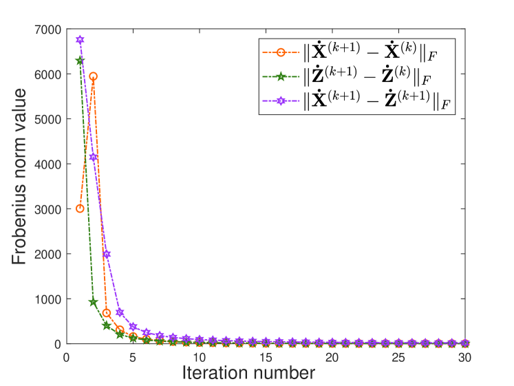
Refer to caption
Figure 1: The convergence curves of โ€–๐—ห™(k+1)โˆ’๐—ห™(k)โ€–Fsubscriptnormsuperscriptห™๐—๐‘˜1superscriptห™๐—๐‘˜๐น\|\mathbf{\dot{X}}^{(k+1)}-\mathbf{\dot{X}}^{(k)}\|_{F}, โ€–๐™ห™(k+1)โˆ’๐™ห™(k)โ€–Fsubscriptnormsuperscriptห™๐™๐‘˜1superscriptห™๐™๐‘˜๐น\|\mathbf{\dot{Z}}^{(k+1)}-\mathbf{\dot{Z}}^{(k)}\|_{F} and โ€–๐—ห™(k+1)โˆ’๐™ห™(k+1)โ€–Fsubscriptnormsuperscriptห™๐—๐‘˜1superscriptห™๐™๐‘˜1๐น\|\mathbf{\dot{X}}^{(k+1)}-\mathbf{\dot{Z}}^{(k+1)}\|_{F} of the proposed QWSNM algorithm. Test image: โ€œBirdโ€.

4 Experimental Results

To demonstrate the effectiveness of our proposed QWSNM algorithm, we carry out extensive experiments on two representative CIR tasks, i.e., color image denoising and deblurring. To evaluate the quality of the restored images, the peak signal to noise ratio (PSNR) and structural similarity (SSIM) 2004Image are chosen as the quantitative metrics. Generally, a higher PSNR value suggests the recovery result is of higher quality, but in some scenarios it may not. To this end, the perceptual quality metric SSIM 2004Image is calculated to evaluate the visual quality. The higher SSIM value indicates the better visual quality. All the experiments were implemented in Matlab 2021b on a desktop with 3.30GHz CPU and 16GB RAM.
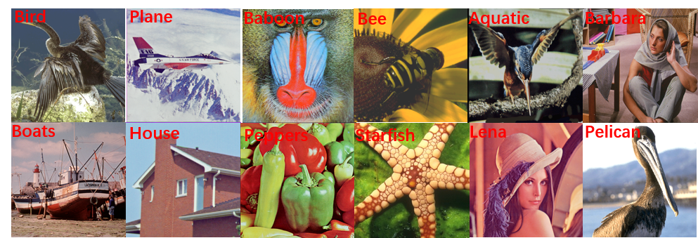
Refer to caption
Figure 2: Images in Set12 wang2019variational .
ย Methods SV-TV jia2019color CBM3D dabov2007image IRCNN zhang2017learning pQSTV wu2022total QWNNM yu2019quaternion QWSNM (Ours)
ฯƒ=15๐œŽ15\sigma=15
Bird 31.16/0.9383 32.54/0.9567 32.96/0.9607 31.17/0.9414 32.77/0.9565 32.86/0.9593
Plane 30.82/0.8940 33.76/0.9554 34.25/0.9573 32.72/0.9382 34.69/0.9598 34.81/0.9607
Baboon 28.14/0.9321 29.59/0.9474 29.96/0.9514 28.68/0.9344 30.18/0.9537 30.24/0.9539
Bee 31.09/0.9394 34.69/0.9647 35.31/0.9696 34.06/0.9606 35.78/0.9729 35.81/0.9733
Aquatic 31.19/0.9093 33.31/0.9491 33.82/0.9517 31.96/0.9335 33.88/0.9532 34.06/0.9537
Barbara 29.64/0.9349 32.67/0.9641 32.57/0.9603 31.57/0.9526 33.14/0.9662 33.24/0.9672
Boat 30.38/0.9132 32.71/0.9631 33.30/0.9672 31.47/0.9501 33.08/0.9659 33.15/0.9661
House 30.82/0.9575 34.85/0.9801 34.07/0.9779 33.42/0.9746 34.74/0.9796 34.72/0.9794
Peppers 28.82/0.9750 32.53/0.9888 32.85/0.9899 32.18/0.9881 33.35/0.9907 33.42/0.9908
Starfish 31.00/0.9718 32.96/0.9862 33.61/0.9879 31.79/0.9822 33.38/0.9866 33.43/0.9869
Lena 32.15/0.9843 33.94/0.9892 33.91/0.9891 33.00/09866 34.13/0.9898 34.15/0.9899
Pelican 31.15/0.9084 32.65/0.9449 32.37/0.9376 31.26/0.9218 32.88/0.9479 32.94/0.9489
Average 30.53/0.9382 33.02/0.9658 33.25/0.9667 31.94/0.9553 33.50/0.9686 33.57/0.9692
ฯƒ=25๐œŽ25\sigma=25
Bird 28.23/0.8875 29.73/0.9225 30.22/0.9311 28.39/0.8973 29.52/0.9223 30.11/0.9291
Plane 28.95/0.8586 31.14/0.8586 31.63/0.9346 30.06/0.9055 32.10/0.9415 32.16/0.9425
Baboon 25.46/0.8650 27.05/0.9032 27.44/0.9132 26.19/0.8827 27.62/0.9145 27.66/0.9166
Bee 29.73/0.9219 32.48/0.9483 32.98/0.9537 31.90/0.9417 33.30/0.9563 33.38/0.9569
Aquatic 28.80/0.8716 30.68/0.9215 31.23/0.9275 29.39/0.8992 31.27/0.9290 31.30/0.9301
Barbara 27.39/0.9006 30.04/0.9390 30.10/0.9376 28.89/0.9212 30.49/0.9445 30.59/0.9455
Boat 28.06/0.8949 29.92/0.9372 30.59/0.9458 28.70/0.9181 30.31/0.9437 30.39/0.9443
House 29.15/0.9479 33.03/0.9721 32.13/0.9694 31.78/0.9649 32.93/0.9717 33.01/0.9719
Peppers 27.09/0.9655 30.06/0.9812 30.46/0.9832 29.51/0.9794 30.84/0.9841 30.92/0.9844
Starfish 28.90/0.9666 30.27/0.9770 30.99/0.9800 28.99/0.9705 30.89/0.9786 30.90/0.9787
Lena 29.78/0.9738 32.27/0.9847 32.30/0.9849 31.42/0.9814 32.49/0.9856 32.55/0.9858
Pelican 27.77/0.8491 30.51/0.9206 30.58/0.9186 29.48/0.8976 30.74/0.9226 30.76/0.9237
Average 28.28/0.9086 30.60/0.9449 30.86/0.9483 29.56/0.9300 31.04/0.9485 31.14/0.9508
ฯƒ=35๐œŽ35\sigma=35
Bird 26.55/0.8869 27.92/0.8869 28.53/0.9022 26.91/0.8574 28.32/0.8974 28.40/0.8996
Plane 27.36/0.7858 29.34/0.9055 29.89/0.9113 28.41/0.8734 30.32/0.9233 30.41/0.9253
Baboon 24.38/0.8278 25.40/0.8555 25.94/0.8718 24.71/0.8329 26.00/0.8726 26.10/0.8779
Bee 28.31/0.8914 30.86/0.9333 31.50/0.9405 30.56/0.9268 31.82/0.9433 31.92/0.9439
Aquatic 27.05/0.8099 28.81/0.8890 29.47/0.9024 27.56/0.8563 29.48/0.9041 29.62/0.9075
Barbara 26.01/0.8682 28.15/0.9120 28.57/0.9179 27.30/0.8937 28.77/0.9219 28.89/0.9237
Boat 26.45/0.8472 28.00/0.9083 28.86/0.9238 27.19/0.8904 28.48/0.9183 28.57/0.9194
House 27.75/0.9283 31.58/0.9636 30.78/0.9617 30.53/0.9564 31.88/0.9659 32.06/0.9668
Peppers 26.04/0.9562 28.19/0.9722 28.88/0.9764 28.02/0.9712 29.21/0.9774 29.30/0.9780
Starfish 27.19/0.9485 28.38/0.9672 29.36/0.9725 27.50/0.9602 29.23/0.9713 29.25/0.9715
Lena 28.60/0.9665 30.91/0.9799 31.16/0.9812 30.22/0.9764 31.30/0.9818 31.38/0.9821
Pelican 26.62/0.8042 29.09/0.8994 29.34/0.9011 28.56/0.8743 29.36/0.9039 29.41/0.9066
Average 26.86/0.8729 28.89/0.9227 29.35/0.9307 28.12/0.9059 29.52/0.9318 29.61/0.9335
ฯƒ=45๐œŽ45\sigma=45
Bird 25.19/0.7892 26.87/0.8602 27.33/0.8743 25.84/0.8179 26.90/0.8594 27.13/0.8684
Plane 26.16/0.8385 28.32/0.8887 28.72/0.8920 27.24/0.8496 29.00/0.9040 29.11/0.9086
Baboon 23.38/0.7797 24.43/0.8150 24.91/0.8431 23.81/0.7951 24.75/0.8278 25.10/0.8512
Bee 27.39/0.8721 30.06/0.9237 30.43/0.9293 29.44/0.9122 30.73/0.9309 30.83/0.9338
Aquatic 25.74/0.7645 27.73/0.8656 28.21/0.8780 26.29/0.8249 28.01/0.8745 28.27/0.8833
Barbara 24.81/0.8349 27.25/0.8658 27.49/0.9015 26.01/0.8689 27.45/0.8988 27.55/0.9035
Boat 25.08/0.8060 26.79/0.8851 27.62/0.9029 25.81/0.8612 26.98/0.8866 27.23/0.8942
House 26.79/0.9120 30.86/0.9584 29.95/0.9547 29.46/0.9455 31.31/0.9620 31.29/0.9619
Peppers 25.19/0.9474 27.02/0.9647 27.74/0.9699 26.83/0.9634 28.01/0.9713 27.97/0.9710
Starfish 25.85/0.9339 27.36/0.9612 28.04/0.9657 26.30/0.9495 28.01/0.9625 28.02/0.9638
Lena 27.37/0.9568 30.26/0.9772 30.29/0.9778 29.21/0.9714 30.18/0.9773 30.37/0.9783
Pelican 25.33/0.7549 28.25/0.8876 28.44/0.8889 27.23/0.8505 28.28/0.8824 28.45/0.8908
Average 25.69/0.8492 27.93/0.9044 28.26/0.9147 26.96/0.8842 28.30/0.9115 28.44/0.9174
Table 2: Comparison of the denoising PSNR (dB) values. The best results are highlighted in bold and the second-best results are underlined.
Refer to caption
(a) Baboon
Refer to caption
(b) (15.08/0.4890)
Refer to caption
(c) (23.38/0.7797)
Refer to caption
(d) (24.43/0.8150)
Refer to caption
(e) (24.91/0.8431)
Refer to caption
(f) (23.81/0.7951)
Refer to caption
(g) (24.75/0.8278)
Refer to caption
(h) (25.10/0.8512)
Figure 3: Denoising performance on โ€œBaboonโ€ with visual quality and numerical results (PSNR/SSIM). (a) Ground truth; (b) Noisy image (ฯƒ=45๐œŽ45\sigma=45); (c) SV-TV jia2019color ; (d) CBM3D dabov2007image ; (e) IRCNN zhang2017learning ; (f) pQSTV wu2022total ; (g) QWNNM yu2019quaternion ; (h) QWSNM (Ours).

4.1 Color Image Denoising

For the color image denoising, the recovery performance is evaluated on the benchmark Set12333The test images of Set12 are mainly collected from Wang et al. wang2019variational . Concretely, Bird, Plane, Baboon, Bee, Aquatic, Barbara, Boat, House, Peppers and Starfish are all with the size of 256ร—256256256256\times 256, Lena and Pelican are with the size of 512ร—512512512512\times 512. dataset, which contains 12 natural RGB color images shown in Fig. 2. All the color noisy images are synthesized by adding the Gaussian noise with mean zero and variance ฯƒ2superscript๐œŽ2\sigma^{2}. To be concrete, we test the scenarios of noise levels ฯƒ๐œŽ\sigma equal to 15, 25, 35 and 45 respectively. In our experiments, we compare our proposed QWSNM algorithm with several prevailing methods, including SV-TV jia2019color , CBM3D dabov2007image , IRCNN zhang2017learning , QWNNM yu2019quaternion , pQSTV wu2022total . Particularly, it is noted that SV-TV, QWNNM and pQSTV are all quaternion-based methods which represent the color image via a pure quaternion matrix to preserve the relationship of three channels. IRCNN zhang2017learning is a convolution neural network method which was trained to handle a wide range of noise levels. CBM3D dabov2007image applies the classical BM3D algorithm to the denoising of color images and its working principle is to convert the color image from the RGB space into a less correlated luminance-chrominance space. For the comparison methods, the involved parameters are all manually-tuned or automatically set up according to the reference papers to achieve the best performance. In our proposed algorithm, parameters that need to be considered include the patch size w๐‘คw, similar patch number M๐‘€M, search window W๐‘ŠW, the power p๐‘p value in the weighted Schatten p๐‘p norm regularizer, the iteration number K๐พK, the parameters c๐‘c and ฯตitalic-ฯต\epsilon in the weight wi=cฯƒiโ€‹(๐—ห™)+ฯตsubscript๐‘ค๐‘–๐‘subscript๐œŽ๐‘–ห™๐—italic-ฯตw_{i}=\frac{c}{\sigma_{i}(\mathbf{\dot{X}})+\epsilon}. For ฯƒโ‰ค40๐œŽ40\sigma\leq 40, we set the search window W๐‘ŠW as 303030. When 0<ฯƒโ‰ค200๐œŽ200<\sigma\leq 20, we set the similar patch number M๐‘€M, the patch size wร—w๐‘ค๐‘คw\times w and the iteration number K๐พK as 707070, 4ร—4444\times 4, and 888, respectively. When 20<ฯƒโ‰ค4020๐œŽ4020<\sigma\leq 40, we set the similar number M๐‘€M, the patch size wร—w๐‘ค๐‘คw\times w and the iteration number K๐พK as 909090, 5ร—5555\times 5, and 121212, respectively. For 40<ฯƒโ‰ค5040๐œŽ5040<\sigma\leq 50, we set the search window W๐‘ŠW, the similar patch number M๐‘€M, the patch size wร—w๐‘ค๐‘คw\times w and the iteration number K๐พK as 404040, 120120120, 5ร—5555\times 5, and 141414, respectively. Throughout the denoising experiments, we fix the power p๐‘p value and the regularization parameter ฮป๐œ†\lambda as 0.950.950.95 and 111 for simplicity. In addition, the parameters c๐‘c and ฯตitalic-ฯต\epsilon are set as 22\sqrt{2} and eps (a Matlab built-in function) respectively, which is as the same as the parameter setting in the WNNM gu2014weighted .

Table 2 reports the PSNR and SSIM values of each image as well as the average results of the competing approaches under different noise levels. The best results are highlighted in bold and the second-best results are underlined. One can observe that our proposed QWSNM algorithm achieves the best objective performance in most cases. For the PSNR metric, our method achieves 0.320.320.32dB, 0.280.280.28dB, 0.260.260.26dB and 0.180.180.18dB improvement over the state-of-the-art approach IRCNN zhang2017learning on average with respect to ฯƒ=15,25,35,45๐œŽ15253545\sigma=15,25,35,45. The main reason behind this phenomenon is that we adopt the quaternion representation, which can better preserve the inter-relationship between RGB channels. Compared with the most similar quaternion-based approach QWNNM yu2019quaternion , our method achieves slight quantitative gain of 0.070.070.07dB, 0.100.100.10dB, 0.090.090.09dB and 0.140.140.14dB on average with respect to ฯƒ=15,25,35,45๐œŽ15253545\sigma=15,25,35,45. A reasonable explanation is that QWNNM yu2019quaternion tends to over-shrink the dominant rank components, which constraints its capacity of recovering the images with rich textures. The above quantitative results fully demonstrate the effectiveness of exploiting both the quaternion representation and WSNM regularization jointly, as in our proposed QWSNM approach. Human subject perception is the ultimate judge of image quality, which also plays a crucial role in the estimation of denoising algorithms. The visual quality comparisons for the test image โ€œBaboonโ€ are shown in Fig. 3. As can be observed from the highlighted window, SV-TV method produces agonizing visual artifacts, while CBM3D, IRCNN and pQSTV approaches are pone to over-smooth the image, losing some of the tiny details. Although QWNNM method overcomes the over-smooth phenomenon, it generates unpleasant visual artifacts. In contrast, our proposed QWSNM approach is not only capable of achieving a better visual perception of both texture and detail information, but also significantly eliminating visual artifacts.

4.2 Color Image Deblurring

In this subsection, we conduct extensive color image deblurring experiments to demonstrate the superiority of our proposed QWSNM. The test images are selected from Set12 and Set27444The test images of Set27 are downloaded from https://github.com/Huang-chao-yan/dataset. Image 1-7 and 16 are with the size of 500ร—500500500500\times 500; Image 8 is with the size of 560ร—392560392560\times 392; Image 9 and 22-25 are with the size of 481ร—321481321481\times 321; Image 10 and 21 are with the size of 1024ร—68310246831024\times 683; Image 11 is with the size of 1024ร—76410247641024\times 764; Image 12 is with the size of 321ร—481321481321\times 481; Image 13 is with the size of 1024ร—70110247011024\times 701; Image 14 is with the size of 1024ร—78310247831024\times 783; Image 15 is with the size of 1024ร—68410246841024\times 684; Image 17 is with the size of 1024ร—60510246051024\times 605; Image 18 is with the size of 448ร—296448296448\times 296; Image 19 is with the size of 256ร—256256256256\times 256; Image 20 is with the size of 288ร—288288288288\times 288; Image 26 is with the size of 418ร—378418378418\times 378; Image 27 is with the size of 1024ร—93710249371024\times 937., which are shown in Figs. 2 and 4, respectively. Three sets of experiments are conducted for simulated color image deblurring. The first is a 9ร—9999\times 9 uniform kernel, the second is a Gaussian kernel with standard variation 1.6, and the third is a motion kernel with motion length 20 and motion angle 60. Then, additive Gaussian noise with ฯƒ=15๐œŽ15\sigma=15 is added to the blurred images. The involved parameters of our algorithm are set as follows: ฮป=65๐œ†65\lambda=65, ฮฒ=7.5๐›ฝ7.5\beta=7.5 for Gaussian blur with noise; ฮป=115๐œ†115\lambda=115, ฮฒ=7.5๐›ฝ7.5\beta=7.5 for motion blur with noise; ฮป=115๐œ†115\lambda=115, ฮฒ=8.5๐›ฝ8.5\beta=8.5 for average blur with noise. Particularly, we fix the search window size W๐‘ŠW, the similar number M๐‘€M and the patch size w๐‘คw as 30, 155 and 6ร—\times6, respectively. Moreover, we study the influence of the parameters c๐‘c and ฯตitalic-ฯต\epsilon in the weight wi=cฯƒiโ€‹(๐—ห™)+ฯตsubscript๐‘ค๐‘–๐‘subscript๐œŽ๐‘–ห™๐—italic-ฯตw_{i}=\frac{c}{\sigma_{i}(\mathbf{\dot{X}})+\epsilon}. Experiments on the test image โ€œBirdโ€ with motion blur and noise are conducted, where c๐‘c is set to [0.1:5]โˆ—2[0.1:5]*\sqrt{2} with an increment of 0.2 and ฯตitalic-ฯต\epsilon is set to [1,250000]โˆ—[1,250000]*eps with step size 10000. As shown in Fig. 4, the parameter ฯตitalic-ฯต\epsilon does not dramatically affect the results and we set ฯต=italic-ฯตabsent\epsilon= eps for all our deblurring experiments. The adjustment of parameter c๐‘c has a greater impact on the results and we set c=2.2โˆ—2๐‘2.22c=2.2*\sqrt{2} for all deblurring experiments through trial and error.

We compare the proposed QWSNM with five representative methods including SV-TV jia2019color , IDD-BM3D danielyan2011bm3d , IRCNN zhang2017learning , MSWNNM yair2018multi and QWNNM* huang2022quaternion . The PSNR and SSIM values of compared deblurring methods with average blur AB(9,9)/ฯƒ=15๐œŽ15\sigma=15 are shown in Table 3. The corresponding results with motion blur MB(20,60)/ฯƒ=15๐œŽ15\sigma=15 and with Gaussian blur GB(25,1.6)/ฯƒ=15๐œŽ15\sigma=15 are reported in Tables 4 and 5, respectively. The best results are highlighted in bold and the second-best results are underlined. As expected, it can be observed that the proposed QWSNM approach consistently generates much better deblurring results on average on different types of blur. Moreover, we display the restored images to demonstrate the perceptual superiority of the proposed method. Figs. 6, 7, 8 show the visual results of these competing methods. For Img26, we can clearly observe that SV-TV, IDD-BM3D, IRCNN and MSWNNM are apt to over-smooth the text image, leading to the characters unrecognized. Although QWNNM approach achieves better visual results than the above four methods, it still tends to generate the over-smooth phenomenon. By contrast, the text image recovered by our proposed QWSNM is sharper and the characters can be better recognized. For Img1, it is evident that SV-TV method generates color distortions and color artifacts, while IDD-BM3D, IRCNN and MSWNNM approaches are prone to over-smooth the image, losing many vital details. Although QWNNM method can prevent the over-smooth phenomenon to some extent, benefiting from the advantages of quaternion representation, it is still not able to recover some of the texture structures. Compared with these competing methods, our proposed QWSNM achieves the best visual results on the whole, which not only preserves more texture structures in the wallpaper of the window, but also effectively eliminates the undesirable color distortions.

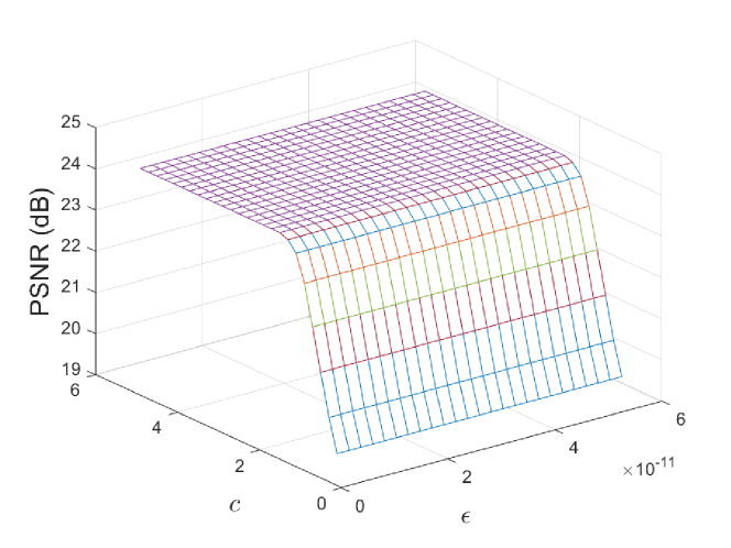
Refer to caption
Figure 4: Images in Set27 huang2022quaternion .
Refer to caption
Figure 5: Evolution of PSNR values with different parameters c๐‘c and ฯตitalic-ฯต\epsilon in the case of motion deblurring. Test image: โ€œBirdโ€.
Refer to caption
(a) Img26
Refer to caption
(b) (15.55/0.8716)
Refer to caption
(c) (17.23/0.9039)
Refer to caption
(d) (18.23/0.9241)
Refer to caption
(e) (19.31/0.9480)
Refer to caption
(f) (19.03/0.9380)
Refer to caption
(g) (20.48/0.9544)
Refer to caption
(h) (21.06/0.9610)
Figure 6: Deblurring performance on โ€œImg26โ€ with visual quality and numerical results (PSNR/SSIM). (a) Ground truth; (b) Degraded image with average kernel (9,9) and Gaussian noise level ฯƒ=15๐œŽ15\sigma=15; Restored image by (c) SV-TV jia2019color ; (d) IDD-BM3D danielyan2011bm3d ; (e) IRCNN zhang2017learning ; (f) MSWNNM yair2018multi ; (g) QWNNM* huang2022quaternion ; (h) QWSNM (Ours).
Refer to caption
(a) Plane
Refer to caption
(b) (21.88/0.4406)
Refer to caption
(c) (24.52/0.7808)
Refer to caption
(d) (26.04/0.8527)
Refer to caption
(e) (27.04/0.8561)
Refer to caption
(f) (27.18/0.8744)
Refer to caption
(g) (27.19/0.8776)
Refer to caption
(h) (27.30/0.8895)
Figure 7: Deblurring performance on โ€œPlaneโ€ with visual quality and numerical results (PSNR/SSIM). (a) Ground truth; (b) Degraded image with Gaussian kernel (25,1.6) and Gaussian noise level ฯƒ=15๐œŽ15\sigma=15; Restored image by (c) SV-TV jia2019color ; (d) IDD-BM3D danielyan2011bm3d ; (e) IRCNN zhang2017learning ; (f) MSWNNM yair2018multi ; (g) QWNNM* huang2022quaternion ; (h) QWSNM (Ours).
Refer to caption
(a) Img1
Refer to caption
(b) (17.47/0.6858)
Refer to caption
(c) (20.89/0.8342)
Refer to caption
(d) (20.66/0.8272)
Refer to caption
(e) (22.58/0.8764)
Refer to caption
(f) (22.56/0.8752)
Refer to caption
(g) (22.56/0.8728)
Refer to caption
(h) (22.92/0.8810)
Figure 8: Deblurring performance on โ€œImg1โ€ with visual quality and numerical results (PSNR/SSIM). (a) Ground truth; (b) Degraded image with motion kernel (20,60) and Gaussian noise level ฯƒ=15๐œŽ15\sigma=15; Restored image by (c) SV-TV jia2019color ; (d) IDD-BM3D danielyan2011bm3d ; (e) IRCNN zhang2017learning ; (f) MSWNNM yair2018multi ; (g) QWNNM* huang2022quaternion ; (h) QWSNM (Ours).
ย Methods SV-TV jia2019color IDD-BM3D danielyan2011bm3d IRCNN zhang2017learning MSWNNM yair2018multi QWNNM* huang2022quaternion QWSNM (Ours)
Set27
Img1 21.50/0.8369 21.47/0.8348 22.68/0.8683 22.66/0.8672 22.83/0.8696 23.17/0.8764
Img2 25.59/0.8497 25.02/0.8460 26.53/0.8714 26.52/0.8712 26.45/0.8712 26.64/0.8724
Img3 21.85/0.7563 20.92/0.7365 23.52/0.8177 23.60/0.8221 23.95/0.8189 24.41/0.8350
Img4 26.31/0.9564 26.07/0.9546 27.42/0.9653 27.45/0.9657 27.68/0.9671 27.81/0.9680
Img5 29.92/0.9710 29.89/0.9716 31.58/0.9806 31.68/0.9808 31.85/0.9815 32.01/0.9823
Img6 23.00/0.8640 22.92/0.8619 23.78/0.8791 23.73/0.8792 24.07/0.8865 24.14/0.8870
Img7 23.76/0.8541 24.36/0.8699 24.99/0.8845 24.93/0.8839 25.25/0.8914 25.34/0.8931
Img8 21.03/0.7982 21.25/0.8430 22.18/0.8658 22.13/0.8398 22.53/0.8686 22.81/0.8694
Img9 28.71/0.9310 28.61/0.9343 28.92/0.9385 28.91/0.9384 28.98/0.9391 29.00/0.9394
Img10 19.65/0.8445 19.59/0.8439 20.30/0.8648 20.26/0.8639 20.57/0.8723 20.63/0.8743
Img11 20.75/0.8124 20.59/0.8071 21.63/0.8414 21.58/0.8386 21.96/0.8502 22.06/0.8536
Img12 21.77/0.5826 21.16/0.5424 21.89/0.5992 21.83/0.5919 21.88/0.5960 21.92/0.5995
Img13 23.59/0.7909 23.27/0.7856 24.43/0.8228 24.38/0.8169 24.65/0.8267 24.71/0.8324
Img14 22.53/0.7253 22.09/0.7085 23.66/0.7786 23.68/0.7807 24.02/0.7885 24.30/0.7978
Img15 27.86/0.9044 27.54/0.9051 28.60/0.9152 28.58/0.9150 28.72/0.9173 28.74/0.9176
Img16 26.01/0.8077 26.58/0.8237 27.46/0.8419 27.46/0.8402 28.08/0.8604 28.18/0.8606
Img17 23.36/0.8375 23.36/0.8375 24.15/08592 24.11/0.8573 24.37/0.8589 24.47/0.8621
Img18 18.97/0.8045 18.78/0.7964 19.21/0.8166 19.15/0.8136 19.42/0.8246 19.48/0.8256
Img19 22.06/0.8944 20.87/0.8584 22.60/0.9038 22.72/0.9065 23.05/0.9069 23.43/0.9191
Img20 26.07/0.9135 26.63/0.9347 27.83/0.9446 27.88/0.9452 27.71/0.9431 27.94/0.9475
Img21 32.12/0.9536 32.52/0.9663 33.71/0.9677 33.73/0.9700 33.24/0.9651 33.30/0.9656
Img22 33.60/0.9458 32.61/0.9524 34.06/0.9607 34.26/0.9619 33.78/0.9526 34.04/0.9544
Img23 23.43/0.8129 23.28/0.8104 23.88/0.8333 23.80/0.8292 24.26/0.8466 24.30/0.8482
Img24 29.27/0.9563 29.14/0.9590 29.69/0.9645 29.65/0.9642 29.55/0.9619 29.64/0.9627
Img25 26.00/0.7769 25.83/0.7733 26.17/0.7843 26.13/0.7810 26.13/0.7807 26.15/0.7814
Img26 17.23/0.9039 18.23/0.9241 19.31/0.9480 19.03/0.9380 20.48/0.9544 21.06/0.9610
Img27 29.13/0.8344 29.12/0.8608 31.14/0.8848 31.10/0.8835 30.67/0.8739 30.84/0.8744
Average 24.63/0.8487 24.51/0.8490 25.60/0.8743 25.59/0.8684 25.76/0.8762 25.94/0.8799
Set12
Bird 23.01/0.7037 22.77/0.6913 23.33/0.7240 23.27/0.7191 23.49/0.7316 23.55/0.7361
Plane 24.24/0.7709 23.80/0.7837 25.00/0.8220 24.98/0.8222 25.12/0.8265 25.22/0.8295
Baboon 22.02/0.6954 21.97/0.6790 22.38/0.7004 22.31/0.6945 22.37/0.6984 22.46/0.7023
Bee 27.03/0.8886 28.11/0.9103 28.67/0.9129 28.75/0.9137 29.09/0.9174 29.20/0.9186
Aquatic 23.26/0.7307 22.89/0.7308 24.06/0.7804 24.03/0.7824 24.11/0.7861 24.28/0.7874
Barbara 22.86/0.7804 22.66/0.7731 23.60/0.8070 23.60/0.8068 23.62/0.8040 23.79/0.8087
Boat 22.38/0.7679 21.71/0.7555 22.98/0.8019 22.93/0.7977 22.96/0.8006 23.17/0.8042
House 26.34/0.9085 26.64/0.9111 28.04/0.9335 28.15/0.9342 28.61/0.9360 28.95/0.9395
Peppers 22.57/0.9251 23.73/0.9298 24.63/0.9413 24.65/0.9415 24.64/0.9405 24.80/0.9440
Starfish 23.15/0.9207 23.02/0.9251 23.86/0.9354 23.83/0.9354 24.03/0.9365 24.15/0.9367
Lena 27.55/0.9575 27.29/0.9560 28.41/0.9643 28.39/0.9639 28.37/0.9640 28.60/0.9654
Pelican 24.58/0.8221 23.93/0.8122 24.85/0.8402 24.75/0.8394 24.92/0.8339 25.04/0.8362
Average 24.08/0.8226 24.04/0.8215 24.98/0.8469 24.97/0.8459 25.11/0.8471 25.27/0.8507
Table 3: PSNR (dB) and SSIM values of different restoration models for AB(9,9)/ฯƒ=15๐œŽ15\sigma=15. The best results are highlighted in bold and the second-best results are underlined.
ย Methods SV-TV jia2019color IDD-BM3D danielyan2011bm3d IRCNN zhang2017learning MSWNNM yair2018multi QWNNM* huang2022quaternion QWSNM (Ours)
Set27
Img1 23.28/0.8822 23.46/0.8822 24.20/0.9052 24.19/0.9056 24.46/0.9075 24.50/0.9089
Img2 27.16/0.8803 27.02/0.8871 28.19/0.8988 28.30/0.9032 28.32/0.9041 28.38/0.9063
Img3 25.12/0.8501 24.53/0.8442 26.84/0.8804 26.78/0.8667 26.80/0.8930 27.15/0.8950
Img4 27.99/0.9690 28.20/0.9702 29.34/0.9764 29.74/0.9787 29.68/0.9785 29.79/0.9791
Img5 31.61/0.9796 32.58/0.9841 33.18/0.9861 33.52/0.9870 33.90/0.9879 33.96/0.9881
Img6 25.03/0.9077 25.00/0.9047 26.17/0.9228 26.18/0.9248 26.24/0.9250 26.31/0.9261
Img7 26.04/0.9074 26.73/0.9171 27.57/0.9303 27.52/0.9311 27.71/0.9339 27.76/0.9350
Img8 22.71/0.8209 23.26/0.8923 23.94/0.8764 23.93/0.7691 24.27/0.8975 24.37/0.8992
Img9 29.57/0.9378 29.50/0.9455 29.69/0.9441 29.77/0.9452 29.90/0.9493 29.96/0.9500
Img10 20.64/0.8724 20.70/0.8749 21.58/0.8963 21.57/0.8960 21.72/0.8998 21.77/0.9013
Img11 21.78/0.8459 21.79/0.8423 22.77/0.8746 22.78/0.8741 22.94/0.8750 23.00/0.8773
Img12 22.81/0.6606 22.12/0.6088 22.95/0.6760 22.93/0.6698 22.85/0.6606 22.90/0.6653
Img13 25.39/0.8491 24.90/0.8347 26.40/0.8760 26.35/0.8750 26.52/0.8776 26.56/0.8786
Img14 24.69/0.8160 24.19/0.7977 25.89/0.8449 25.83/0.8432 26.14/0.8604 26.25/0.8619
Img15 29.25/0.9241 29.01/0.9225 29.85/0.9293 29.80/0.9279 30.13/0.9373 30.19/0.9378
Img16 28.16/0.8641 29.37/0.8897 30.12/0.8979 30.10/0.8965 30.76/0.9108 30.80/0.9114
Img17 24.51/0.8674 24.67/0.8682 25.45/0.8806 25.40/0.8785 25.64/0.8869 25.67/0.8875
Img18 20.44/0.8585 20.28/0.8523 20.90/0.8747 20.86/0.8722 21.01/0.8776 21.06/0.8791
Img19 24.85/0.9386 23.93/0.9248 25.70/0.9494 25.69/0.9489 25.27/0.9444 25.44/0.9459
Img20 28.10/0.9310 29.60/0.9626 30.58/0.9597 30.56/0.9588 30.84/0.9676 30.87/0.9688
Img21 33.50/0.9624 34.15/0.9743 34.37/0.9684 34.35/0.9678 35.01/0.9757 34.90/0.9743
Img22 34.47/0.9306 34.81/0.9658 35.33/0.9439 35.45/0.9500 35.84/0.9635 35.76/0.9600
Img23 25.55/0.8834 25.44/0.8784 26.30/0.9022 26.38/0.9025 26.60/0.9065 26.62/0.9071
Img24 30.06/0.9603 29.85/0.9655 30.41/0.9667 30.45/0.9672 30.51/0.9698 30.54/0.9701
Img25 26.42/0.7889 26.25/0.7826 26.50/0.7918 26.39/0.7912 26.48/0.7916 26.52/0.7920
Img26 19.56/0.9405 21.99/0.9689 22.84/0.9740 22.69/0.9658 23.35/0.9777 23.60/0.9791
Img27 31.18/0.8735 31.12/0.8925 32.77/0.8883 32.70/0.8856 32.89/0.9084 32.96/0.9098
Average 26.29/0.8853 26.46/0.8903 27.40/0.9044 27.43/0.9007 27.62/0.9099 27.69/0.9109
Set12
Bird 24.52/0.7808 24.47/0.7736 25.12/0.8080 25.14/0.8084 25.20/0.8093 25.27/0.8130
Plane 25.90/0.8014 26.04/0.8527 27.04/0.8561 27.18/0.8744 27.19/0.8776 27.30/0.8895
Baboon 22.97/0.7466 22.98/0.7282 23.42/0.7617 23.36/0.7533 23.43/0.7516 23.48/0.7572
Bee 28.66/0.9039 30.26/0.9308 30.65/0.9293 30.98/0.9363 31.32/0.9391 31.42/0.9455
Aquatic 25.09/0.7961 25.37/0.8271 26.30/0.8486 26.42/0.8638 26.51/0.8669 26.58/0.8702
Barbara 24.15/0.8275 24.27/0.8301 24.91/0.8530 24.94/0.8543 24.92/0.8517 25.00/0.8585
Boat 23.68/0.8086 23.62/0.8365 24.71/0.8501 24.74/0.8534 24.55/0.8504 24.62/0.8585
House 27.32/0.9242 28.61/0.9402 29.10/0.9456 29.12/0.9460 29.82/0.9496 29.90/0.9500
Peppers 25.55/0.9501 25.94/0.9561 26.65/0.9622 26.64/0.9620 26.57/0.9615 26.69/0.9643
Starfish 25.15/0.9388 25.47/0.9487 26.60/0.9557 26.65/0.9560 26.67/0.9596 26.77/0.9654
Lena 29.06/0.9684 29.27/0.9691 30.27/0.9754 30.24/0.9750 30.48/0.9761 30.55/0.9800
Pelican 25.70/0.8403 25.15/0.8412 26.18/0.8610 26.16/0.8605 26.13/0.8602 26.26/0.8701
Average 25.65/0.8572 25.95/0.8687 26.75/0.8839 26.80/0.8870 26.90/0.8878 26.98/0.8931
Table 4: PSNR (dB) and SSIM values of different restoration models for GB(25,1.6)/ฯƒ=15๐œŽ15\sigma=15. The best results are highlighted in bold and the second-best results are underlined.
ย Methods SV-TV jia2019color IDD-BM3D danielyan2011bm3d IRCNN zhang2017learning MSWNNM yair2018multi QWNNM* huang2022quaternion QWSNM (Ours)
Set27
Img1 20.89/0.8342 20.66/0.8272 22.58/0.8764 22.56/0.8752 22.55/0.8728 22.92/0.8810
Img2 24.96/0.8331 24.20/0.8279 26.13/0.8668 26.13/0.8660 26.19/0.8695 26.35/0.8715
Img3 22.05/0.7712 20.01/0.7163 24.05/0.8387 24.14/0.8399 24.06/0.8359 24.24/0.8412
Img4 26.47/0.9591 26.03/0.9561 27.77/0.9684 27.80/0.9687 28.22/0.9712 28.28/0.9714
Img5 29.47/0.9695 29.13/0.9691 31.08/0.9788 31.11/0.9787 31.68/0.9816 31.83/0.9820
Img6 22.59/0.8520 22.29/0.8458 23.62/0.8755 23.57/0.8741 23.88/0.8815 23.99/0.8833
Img7 22.50/0.8231 23.05/0.8408 24.23/0.8703 24.16/0.8690 24.56/0.8799 24.71/0.8834
Img8 20.40/0.7541 20.80/0.8098 21.79/0.8535 21.74/0.7293 22.17/0.9099 22.48/0.9352
Img9 28.14/0.9202 27.93/0.9251 28.61/0.9360 28.55/0.9350 28.58/0.9349 28.59/0.9351
Img10 19.48/0.8410 19.23/0.8370 20.29/0.8647 20.24/0.8632 20.58/0.8728 20.65/0.8748
Img11 20.30/0.8028 19.92/0.7916 21.33/0.8362 21.27/0.8330 21.56/0.8435 21.76/0.8470
Img12 21.62/0.5859 20.84/0.5268 21.83/0.6056 21.75/0.5968 21.72/0.5975 21.82/0.5984
Img13 23.27/0.7840 22.56/0.7680 24.35/0.8222 24.27/0.8160 24.42/0.8224 24.59/0.8260
Img14 22.04/0.7166 21.15/0.6841 23.49/0.7790 23.49/0.7782 23.79/0.7840 24.13/0.7979
Img15 27.07/0.8937 26.36/0.8883 27.98/0.9097 27.93/0.9092 28.04/0.9070 28.19/0.9160
Img16 25.57/0.7891 25.71/0.8053 27.01/0.8327 27.01/0.8300 27.19/0.8436 27.66/0.8533
Img17 22.81/0.8187 22.58/0.8149 23.92/0.8478 23.88/0.8449 24.15/0.8467 24.32/0.8515
Img18 19.29/0.8263 18.87/0.8119 19.63/0.8408 19.56/0.8375 19.90/0.8507 19.96/0.8521
Img19 20.99/0.8738 19.19/0.8249 22.24/0.9006 22.33/0.9021 22.06/0.8943 22.27/0.8995
Img20 24.82/0.8786 25.09/0.9105 26.94/0.9377 26.94/0.9378 26.75/0.9357 27.03/0.9394
Img21 31.52/0.9483 31.60/0.9591 33.34/0.9670 33.35/0.9672 32.67/0.9611 32.75/0.9613
Img22 32.56/0.9247 30.88/0.9362 33.38/0.9594 33.47/0.9580 33.75/0.9549 33.81/0.9556
Img23 23.21/0.8145 22.88/0.8051 23.72/0.8366 23.64/0.8314 24.26/0.8542 24.32/0.8549
Img24 28.70/0.9483 28.57/0.9526 29.31/0.9604 29.24/0.9601 29.16/0.9578 29.17/0.9582
Img25 25.84/0.7787 25.63/0.7715 26.16/0.7884 26.07/0.7820 26.05/0.7831 26.08/0.7835
Img26 17.26/0.9082 18.42/0.9311 19.92/0.9496 19.68/0.9487 22.02/0.9705 22.08/0.9708
Img27 28.35/0.8276 27.05/0.8296 30.54/0.8824 30.50/0.8810 30.02/0.8649 30.32/0.8700
Average 24.15/0.8399 23.73/0.8358 25.38/0.8735 25.35/0.8685 25.56/0.8753 25.72/0.8813
Set12
Bird 22.77/0.6867 22.37/0.6725 23.34/0.7266 23.25/0.7186 23.59/0.7417 23.62/0.7425
Plane 23.60/0.7149 23.16/0.7555 24.67/0.8134 24.66/0.8123 24.75/0.8196 24.83/0.8212
Baboon 21.70/0.6936 21.74/0.6730 22.16/0.7003 22.08/0.6912 22.26/0.7018 22.30/0.7024
Bee 25.48/0.8554 26.59/0.8868 27.97/0.9064 28.02/0.9066 28.63/0.9130 28.75/0.9140
Aquatic 22.77/0.6857 22.25/0.6919 23.91/0.7730 23.87/0.7732 24.16/0.7792 24.25/0.7835
Barbara 22.59/0.7728 22.44/0.7701 23.44/0.8113 23.40/0.8080 23.64/0.8168 23.74/0.8199
Boat 22.02/0.7383 21.11/0.7355 23.00/0.8068 22.93/0.8032 22.95/0.8043 23.03/0.8072
House 25.04/0.8795 25.02/0.8845 26.33/0.9132 26.46/0.9145 27.82/0.9275 28.00/0.9300
Peppers 23.15/0.9174 23.31/0.9257 24.56/0.9410 24.54/0.9405 24.42/0.9381 24.61/0.9412
Starfish 22.55/0.9069 22.15/0.9133 23.51/0.9339 23.47/0.9337 23.87/0.9368 23.95/0.9381
Lena 27.55/0.9564 27.05/0.9571 28.66/0.9674 28.65/0.9670 28.63/0.9672 28.73/0.9678
Pelican 24.36/0.8167 23.16/0.8000 24.88/0.8438 24.79/0.8420 25.03/0.8399 25.07/0.8405
Average 23.63/0.8020 23.36/0.8055 24.71/0.8448 24.68/0.8426 24.98/0.8489 25.07/0.8506
Table 5: PSNR (dB) and SSIM values of different restoration models for MB(20,60)/ฯƒ=15๐œŽ15\sigma=15. The best results are highlighted in bold and the second-best results are underlined.
ย p๐‘p value p=0.15๐‘0.15p=0.15 p=0.25๐‘0.25p=0.25 p=0.35๐‘0.35p=0.35 p=0.45๐‘0.45p=0.45 p=0.55๐‘0.55p=0.55 p=0.65๐‘0.65p=0.65 p=0.75๐‘0.75p=0.75 p=0.85๐‘0.85p=0.85 p=0.95๐‘0.95p=0.95 p=1๐‘1p=1
MB(20,60)/ฯƒ=15๐œŽ15\sigma=15
Bird 19.28/0.4117 19.28/0.4117 19.28/0.4117 19.28/0.4117 19.28/0.4117 19.33/0.4144 19.51/0.4272 20.26/0.4818 23.62/0.7425 23.41/0.7270
Plane 19.36/0.3255 19.36/0.3255 19.36/0.3255 19.36/0.3255 19.36/0.3255 19.40/0.3278 19.59/0.3389 20.37/0.3913 24.83/0.8212 24.63/0.8125
Baboon 19.06/0.5565 19.06/0.556 19.06/0.556 19.06/0.556 19.06/0.556 19.09/0.5582 19.26/0.5663 19.92/05977 22.30/0.7018 22.21/0.6928
Bee 20.39/0.6448 20.39/0.6448 20.39/0.6448 20.39/0.6448 20.39/0.6448 20.44/0.6469 20.70/0.6567 21.75/0.6985 28.75/0.9140 28.47/0.9117
Aquatic 18.59/0.3513 18.59/0.3513 18.59/0.3513 18.59/0.3513 18.59/0.3513 18.62/0.3535 18.78/0.3639 19.39/0.4101 24.25/0.7835 23.86/0.7690
Barbara 19.16/0.5531 19.16/0.5531 19.16/0.5531 19.16/0.5531 19.16/0.5531 19.20/0.5555 19.38/0.5664 20.07/0.6108 23.74/0.8199 23.65/0.8164
Boat 18.32/0.4328 18.32/0.4238 18.32/0.4238 18.32/0.4238 18.32/0.4238 18.35/0.4262 18.50/0.4375 19.07/0.4874 23.03/0.8072 22.50/0.7895
House 19.65/0.6424 19.65/0.6424 19.65/0.6424 19.65/0.6424 19.65/0.6424 19.69/0.6452 19.91/0.6584 20.77/0.7109 28.00/0.9300 27.19/0.9215
Peppers 19.24/0.8107 19.24/0.8107 19.24/0.8107 19.24/0.8107 19.24/0.8107 19.28/0.8123 19.46/0.8194 20.17/0.8463 24.61/0.9412 24.56/0.9415
Starfish 19.81/0.7516 19.81/0.7516 19.81/0.7516 19.81/0.7516 19.81/0.7516 18.94/0.7536 19.11/0.7622 19.77/0.7965 23.95/0.9381 23.71/0.9363
Lena 20.94/0.8271 20.94/0.8271 20.94/0.8271 20.94/0.8271 20.94/0.8271 21.00/0.8292 21.29/0.8386 22.52/0.8745 28.73/0.9678 28.63/0.9671
Pelican 19.56/0.4135 19.56/0.4135 19.56/0.4135 19.56/0.4135 19.56/0.4135 19.60/0.4161 19.80/0.4256 20.65/0.4839 25.07/0.8405 24.75/0.8332
AB(9,9)/ฯƒ=15๐œŽ15\sigma=15
Bird 20.33/0.4712 20.33/0.4712 20.33/0.4712 20.33/0.4712 20.34/0.4717 20.39/0.4756 20.65/0.4946 21.74/0.5868 23.55/0.7361 23.41/0.7247
Plane 20.69/0.3765 20.69/0.3765 20.69/0.3765 20.69/0.3765 20.70/0.3770 20.76/0.3808 21.04/0.3997 22.36/0.5058 25.22/0.8295 25.07/0.8224
Baboon 19.90/0.5806 19.90/0.5806 19.90/0.5806 19.90/0.5806 19.91/0.5809 19.95/0.5832 20.17/0.5936 21.06/0.6448 22.46/0.7023 22.36/0.6927
Bee 22.11/0.6941 22.11/0.6941 22.11/0.6941 22.11/0.6941 22.11/0.6941 22.19/0.6973 22.59/0.7116 24.24/0.7698 29.20/0.9186 29.20/0.9126
Aquatic 19.97/0.4135 19.97/0.4135 19.97/0.4135 19.97/0.4135 19.99/0.4142 20.04/0.4178 20.27/0.4350 21.45/0.5222 24.28/0.7874 24.15/0.7849
Barbara 20.08/0.5912 20.08/0.5912 20.08/0.5912 20.08/0.5912 20.09/0.5914 20.14/0.5945 20.37/0.6092 21.40/0.6745 23.79/0.8087 23.53/0.8053
Boat 19.55/0.4805 19.55/0.4805 19.55/0.4805 19.55/0.4805 19.56/0.4817 19.61/0.4852 19.82/0.5027 20.94/0.5942 23.17/0.8042 22.92/0.7976
House 21.51/0.7215 21.51/0.7215 21.51/0.7215 21.51/0.7215 21.52/0.7230 21.60/0.7267 21.95/0.7437 23.58/0.8137 28.95/0.9395 28.74/0.9369
Peppers 20.48/0.8458 20.48/0.8458 20.48/0.8458 20.48/0.8458 20.49/0.8467 20.55/0.8486 20.80/0.8569 21.96/0.8893 24.80/0.9440 24.72/0.9433
Starfish 20.35/0.7915 20.35/0.7915 20.35/0.7915 20.35/0.7915 20.36/0.7930 20.41/0.7954 21.66/0.8066 22.76/0.8485 24.15/0.9367 24.06/0.9373
Lena 22.19/0.9601 22.19/0.8601 22.19/0.860 22.19/0.860 22.20/0.8604 22.29/0.8628 22.70/0.8738 24.30/0.9104 28.60/0.9654 28.49/0.9646
Pelican 20.85/0.4638 20.85/0.4638 20.85/0.4638 20.85/0.4638 20.85/0.4638 20.91/0.4683 21.21/0.4874 22.44/0.5740 25.04/0.8362 24.95/0.8215
GB(25,1.6)/ฯƒ=15๐œŽ15\sigma=15
Bird 21.14/0.5421 21.14/0.5421 21.14/0.5421 21.14/0.5421 21.14/0.5421 21.21/0.5460 21.88/0.4406 23.05/0.6712 25.27/0.8130 24.98/0.7967
Plane 21.62/0.4285 21.62/0.4285 21.62/0.4285 21.62/0.4285 21.62/0.4285 21.69/0.4320 22.04/0.4494 23.89/0.5663 27.30/0.8895 26.86/0.8692
Baboon 20.54/0.6377 20.54/0.6377 20.54/0.6377 20.54/0.6377 20.54/0.6377 20.59/0.6400 20.84/0.6508 22.02/0.7096 23.48/0.7572 23.23/0.7376
Bee 22.45/0.7063 22.45/0.7063 22.45/0.7063 22.45/0.7063 22.45/0.7063 22.54/0.7090 22.97/0.7224 25.26/0.7944 31.27/0.9386 31.17/0.9375
Aquatic 21.34/0.4930 21.34/0.4930 21.34/0.4930 21.34/0.4930 21.34/0.4930 21.40/0.4965 21.71/0.5139 23.36/0.6185 26.58/0.8702 26.32/0.8597
Barbara 20.92/0.6405 20.92/0.6405 20.92/0.6405 20.92/0.6405 20.92/0.6405 20.97/0.6435 21.25/0.6581 22.61/0.7336 25.00/0.8585 24.81/0.8476
Boat 20.60/0.5385 20.60/0.5385 20.60/0.5385 20.60/0.5385 20.60/0.5385 20.66/0.5419 20.92/0.5584 22.32/0.6579 24.62/0.8524 24.20/0.8401
House 22.01/0.7448 22.01/0.7448 22.01/0.7448 22.01/0.7448 22.01/0.7448 22.08/0.7483 22.47/0.7649 24.54/0.8443 29.90/0.9500 29.61/0.9475
Peppers 21.49/0.8720 21.49/0.8720 21.49/0.8720 21.49/0.8720 21.49/0.8720 21.55/0.8738 21.88/0.8820 23.51/0.9179 26.63/0.9643 26.40/0.9604
Starfish 21.49/0.8123 21.49/0.8123 21.49/0.8123 21.49/0.8123 21.49/0.8123 21.55/0.8144 21.87/0.8250 23.53/0.8763 26.77/0.9654 26.46/0.9581
Lena 22.46/0.8675 22.46/0.8675 22.46/0.8675 22.46/0.8675 22.46/0.8675 22.52/0.8683 22.95/0.8789 25.21/0.9247 30.55/0.9800 30.27/0.9750
Pelican 21.29/0.4810 21.29/0.4810 21.29/0.4810 21.29/0.4810 21.29/0.4810 21.35/0.4820 21.68/0.4994 23.36/0.6044 26.26/0.8701 26.05/0.8615
Table 6: PSNR (dB) and SSIM values of different p๐‘p values for color image deblurring on the Set12 dataset. The best results are marked in bold.
Refer to caption
(a) ฯƒ๐œŽ\sigma=15
Refer to caption
(b) ฯƒ๐œŽ\sigma=25
Refer to caption
(c) ฯƒ๐œŽ\sigma=35
Refer to caption
(d) ฯƒ๐œŽ\sigma=45
Figure 9: The influence of changing p๐‘p values on denoised results under different noise levels ฯƒ๐œŽ\sigma. Test image: โ€œBirdโ€.
Refer to caption
Refer to caption
Figure 10: The evolution curves of (a) relative error and (b) PSNR value between consecutive iterations in the case of deblurring. Test image: โ€œBirdโ€.

4.3 Analysis of Power p๐‘p

In this part, the effects of power p๐‘p in the weighted Schatten p๐‘p-norm are studied. Table 6 reports the PSNR and SSIM values for deblurring with the power p๐‘p ranging from 0.15 to 1 in the Set12 dataset. From the Table 6, it can be observed that the recovery performance of our method is relatively sensitive to the parameter p๐‘p. When p๐‘p is 0.95, the PSNR and SSIM of QWSNM on all test images consistently achieve the highest values. Therefore, p๐‘p value of 0.95 is a reasonable choice for color image deblurring. To illustrate the influence of p๐‘p values under different noise levels for color image denoising, we just utilize the test image โ€œBirdโ€ as an example and the results are presented in Fig. 9. In each subfigure, the vertical coordinate represents the PSNR value under a certain noise level, while the horizontal coordinate denotes the values of p๐‘p ranging from 0.1 to 1 with interval 0.05. It can be seen that when p๐‘p is 0.95, our algorithm consistently achieve the highest PSNR values under different noise levels. Therefore, we also select p=0.95๐‘0.95p=0.95 for color image denoising.

4.4 Convergence Study

Fig. 10 illustrates the empirical convergence of our proposed algorithm in the cases of three blur kernels on the test image โ€œBirdโ€. One can clearly observe that with the growth of iteration number, all the relative error and PSNR curves decrease and increase monotonically and ultimately become flat and stable, numerically exhibiting the reliable convergence behavior of proposed QWSNM algorithm. It is noted that other scenarios also have the similar conclusions.

5 Conclusion

In this paper, we proposed a quaternion-based QWSNM model for color image restoration, which combines the advantages of the WSNM regularizer and quaternion representation. To be concrete, the WSNM regularizer can better adaptively shrink the rank components over the WNNM counterpart, and the quaternion representation of color images is capable of fully preserving the correlation of three color channels. In particular, we modified the QADMM algorithm through a continuation strategy to iteratively solve the resulting optimization problem. Moreover, rigorous convergence analysis was provided to verify the sound properties of our proposed algorithm. Experimental results on color image denoising under different noise levels and color image deblurring under three types of blur kernels demonstrated the effectiveness and robustness of QWSNM. Compared with the related competing methods, the visual results showed that our proposed QWSNM is capable of better preserving the color structure and avoiding color distortion.

However, despite the good recovery performance, our proposed algorithm has the efficiency limitation. In fact, the QSVD in the optimization process is quite time-consuming, so how to improve the algorithmic efficiency remains a significant issue. Very recently, Gai et al. gai2023theory introduced the theory of reduced biquaternion sparse representation, which benefited from the commutative of the reduced biquaternion algebra. In the future research, we would pay more attention to the reduced biquaternion representation and extend existing algorithms to the reduced biquaternion domain for color image restoration. In parallel, we plan to extend the proposed QWNNM algorithm to other relevant tasks, such as color image inpainting, color image super-resolution and compressive sensing, etc.

Acknowledgements

The research was supported by the NSFC under Grants 12001005, 12271083.

Conflict of Interest

The authors declare that they have no known competing financial interests or personal relationships that could have appeared to influence the work reported in this paper.

Code Availability

Code generated or used during the study are available from the corresponding author on reasonable request.

References

  • (1) Rudin, L.I., Osher, S., Fatemi, E.: Nonlinear total variation based noise removal algorithms. Physica D: Nonlinear Phenomena 60(1-4), 259โ€“268 (1992)
  • (2) Wang, Y., Yang, J., Yin, W., Zhang, Y.: A new alternating minimization algorithm for total variation image reconstruction. SIAM Journal on Imaging Sciences 1(3), 248โ€“272 (2008)
  • (3) Bredies, K., Kunisch, K., Pock, T.: Total generalized variation. SIAM Journal on Imaging Sciences 3(3), 492โ€“526 (2010)
  • (4) Chang, H., Zhang, X., Tai, X.C., Yang, D.: Domain decomposition methods for nonlocal total variation image restoration. Journal of Scientific Computing 60, 79โ€“100 (2014)
  • (5) Mairal, J., Elad, M., Sapiro, G.: Sparse representation for color image restoration. IEEE Transactions on Image Processing 17(1), 53โ€“69 (2007)
  • (6) Zhang, J., Zhao, D., Gao, W.: Group-based sparse representation for image restoration. IEEE Transactions on Image Processing 23(8), 3336โ€“3351 (2014)
  • (7) Zha, Z., Yuan, X., Wen, B., Zhang, J., Zhu, C.: Nonconvex structural sparsity residual constraint for image restoration. IEEE Transactions on Cybernetics 52(11), 12440โ€“12453 (2021)
  • (8) Buades, A., Coll, B., Morel, J.M.: A non-local algorithm for image denoising. In: Proceedings of the IEEE Conference on Computer Vision and Pattern Recognition (CVPR), pp. 60โ€“65 (2005)
  • (9) Danielyan, A., Katkovnik, V., Egiazarian, K.: BM3D frames and variational image deblurring. IEEE Transactions on Image Processing 21(4), 1715โ€“1728 (2011)
  • (10) Peng, Y., Suo, J., Dai, Q., Xu, W.: Reweighted low-rank matrix recovery and its application in image restoration. IEEE Transactions on Cybernetics 44(12), 2418โ€“2430 (2014)
  • (11) Dong, W., Shi, G., Li, X.: Nonlocal image restoration with bilateral variance estimation: a low-rank approach. IEEE Transactions on Image Processing 22(2), 700โ€“711 (2012)
  • (12) Lai, R., Li, J.: Manifold based low-rank regularization for image restoration and semi-supervised learning. Journal of Scientific Computing 74, 1241โ€“1263 (2018)
  • (13) Zhang, K., Li, Y., Zuo, W., Zhang, L., Vanย Gool, L., Timofte, R.: Plug-and-play image restoration with deep denoiser prior. IEEE Transactions on Pattern Analysis and Machine Intelligence 44(10), 6360โ€“6376 (2021)
  • (14) He, L., Zhang, Q., Yang, X., Wang, Y., Wang, C.: SLN-RED: Regularization by simultaneous local and nonlocal denoising for image restoration. IEEE Signal Processing Letters 30, 578โ€“582 (2023)
  • (15) He, W., Zhang, H., Zhang, L., Shen, H.: Total-variation-regularized low-rank matrix factorization for hyperspectral image restoration. IEEE Transactions on Geoscience and Remote Sensing 54(1), 178โ€“188 (2015)
  • (16) Chi, Y., Lu, Y.M., Chen, Y.: Nonconvex optimization meets low-rank matrix factorization: An overview. IEEE Transactions on Signal Processing 67(20), 5239โ€“5269 (2019)
  • (17) Shi, C., Huang, Z., Wan, L., Xiong, T.: Low-rank tensor completion based on log-det rank approximation and matrix factorization. Journal of Scientific Computing 80(3), 1888โ€“1912 (2019)
  • (18) Ke, Y., Ma, C., Jia, Z., Xie, Y., Liao, R.: Quasi non-negative quaternion matrix factorization with application to color face recognition. Journal of Scientific Computing 95(2), 38 (2023)
  • (19) Candรจs, E.J., Li, X., Ma, Y., Wright, J.: Robust principal component analysis? Journal of the ACM 58(3), 1โ€“37 (2011)
  • (20) Jin, Z.F., Wan, Z., Jiao, Y., Lu, X.: An alternating direction method with continuation for nonconvex low rank minimization. Journal of Scientific Computing 66, 849โ€“869 (2016)
  • (21) Yuan, W., Liu, H., Liang, L., Xie, G., Zhang, Y., Liu, D.: Rank minimization via adaptive hybrid norm for image restoration. Signal Processing 206, 108926 (2023)
  • (22) Candes, E., Recht, B.: Exact matrix completion via convex optimization. Communications of the ACM 55(6), 111โ€“119 (2012)
  • (23) Gu, S., Zhang, L., Zuo, W., Feng, X.: Weighted nuclear norm minimization with application to image denoising. In: Proceedings of the IEEE Conference on Computer Vision and Pattern Recognition (CVPR), pp. 2862โ€“2869 (2014)
  • (24) Gu, S., Xie, Q., Meng, D., Zuo, W., Feng, X., Zhang, L.: Weighted nuclear norm minimization and its applications to low level vision. International Journal of Computer Vision 121(2), 183โ€“208 (2017)
  • (25) Nie, F., Huang, H., Ding, C.: Low-rank matrix recovery via efficient Schatten p๐‘p-norm minimization. In: Proceedings of the AAAI Conference on Artificial Intelligence, vol.ย 26, pp. 655โ€“661 (2012)
  • (26) Xie, Y., Gu, S., Liu, Y., Zuo, W., Zhang, W., Zhang, L.: Weighted Schatten p๐‘p-norm minimization for image denoising and background subtraction. IEEE Transactions on Image Processing 25(10), 4842โ€“4857 (2016)
  • (27) Zha, Z., Zhang, X., Wu, Y., Wang, Q., Liu, X., Tang, L., Yuan, X.: Non-convex weighted lpsubscript๐‘™๐‘l_{p} nuclear norm based ADMM framework for image restoration. Neurocomputing 311, 209โ€“224 (2018)
  • (28) Luisier, F., Blu, T.: SURE-LET multichannel image denoising: Interscale orthonormal wavelet thresholding. IEEE Transactions on Image Processing 17(4), 482โ€“492 (2008)
  • (29) Dabov, K., Foi, A., Katkovnik, V., Egiazarian, K.: Image denoising by sparse 3-D transform-domain collaborative filtering. IEEE Transactions on Image Processing 16(8), 2080โ€“2095 (2007)
  • (30) Xu, J., Zhang, L., Zhang, D., Feng, X.: Multi-channel weighted nuclear norm minimization for real color image denoising. In: Proceedings of the IEEE International Conference on Computer Vision (ICCV), pp. 1096โ€“1104 (2017)
  • (31) Huang, X., Du, B., Liu, W.: Multichannel color image denoising via weighted Schatten p๐‘p-norm minimization. In: Proceedings of the Twenty-Ninth International Joint Conferences on Artificial Intelligence (IJCAI), pp. 637โ€“644 (2021)
  • (32) Chen, Y., Xiao, X., Zhou, Y.: Low-rank quaternion approximation for color image processing. IEEE Transactions on Image Processing 29, 1426โ€“1439 (2019)
  • (33) Liu, X., Chen, Y., Peng, Z., Wu, J., Wang, Z.: Infrared image super-resolution reconstruction based on quaternion fractional order total variation with lpsubscript๐‘™๐‘l_{p} quasinorm. Applied Sciences 8(10), 1864 (2018)
  • (34) Miao, J., Kou, K.I.: Color image recovery using low-rank quaternion matrix completion algorithm. IEEE Transactions on Image Processing 31, 190โ€“201 (2021)
  • (35) Zou, C., Kou, K.I., Wang, Y.: Quaternion collaborative and sparse representation with application to color face recognition. IEEE Transactions on Image Processing 25(7), 3287โ€“3302 (2016)
  • (36) Yu, Y., Zhang, Y., Yuan, S.: Quaternion-based weighted nuclear norm minimization for color image denoising. Neurocomputing 332, 283โ€“297 (2019)
  • (37) Huang, C., Li, Z., Liu, Y., Wu, T., Zeng, T.: Quaternion-based weighted nuclear norm minimization for color image restoration. Pattern Recognition 128, 108665 (2022)
  • (38) Huang, C., Li, J., Gao, G.: Review of quaternion-based color image processing methods. Mathematics 11(9), 2056 (2023)
  • (39) Flamant, J., Miron, S., Brie, D.: A general framework for constrained convex quaternion optimization. IEEE Transactions on Signal Processing 70, 254โ€“267 (2021)
  • (40) Jia, Z., Ng, M.K.: Structure preserving quaternion generalized minimal residual method. SIAM Journal on Matrix Analysis and Applications 42(2), 616โ€“634 (2021)
  • (41) Zhang, F.: Quaternions and matrices of quaternions. Linear Algebra and its Applications 251, 21โ€“57 (1997)
  • (42) Mei, J.J., Dong, Y., Huang, T.Z., Yin, W.: Cauchy noise removal by nonconvex ADMM with convergence guarantees. Journal of Scientific Computing 74, 743โ€“766 (2018)
  • (43) He, L., Wang, Y., Gao, S.: A support-denoiser-driven framework for single image restoration. Journal of Computational and Applied Mathematics 393, 113495 (2021)
  • (44) Hou, R., Li, F., Zhang, G.: Truncated residual based plug-and-play ADMM algorithm for MRI reconstruction. IEEE Transactions on Computational Imaging 8, 96โ€“108 (2022)
  • (45) Tao, M., Zhang, X.P.: Study on L1subscript๐ฟ1{L}_{1} over L2subscript๐ฟ2{L}_{2} minimization for nonnegative signal recovery. Journal of Scientific Computing 95(3), 94 (2023)
  • (46) Wu, Z.C., Huang, T.Z., Deng, L.J., Vivone, G.: A framelet sparse reconstruction method for pansharpening with guaranteed convergence. Inverse Problems and Imaging pp. 0โ€“0 (2023)
  • (47) Wu, Z.C., Huang, T.Z., Deng, L.J., Huang, J., Chanussot, J., Vivone, G.: LRTCFPan: Low-rank tensor completion based framework for pansharpening. IEEE Transactions on Image Processing 32, 1640โ€“1655 (2023)
  • (48) Boyd, S., Parikh, N., Chu, E., Peleato, B., Eckstein, J., etย al.: Distributed optimization and statistical learning via the alternating direction method of multipliers. Foundations and Trendsยฎ in Machine learning 3(1), 1โ€“122 (2011)
  • (49) Sangwine, S.J.: Fourier transforms of colour images using quaternion or hypercomplex, numbers. Electronics Letters 32(21), 1979โ€“1980 (1996)
  • (50) Liu, L., Huang, W., Chen, D.R.: Exact minimum rank approximation via Schatten p๐‘p-norm minimization. Journal of Computational and Applied Mathematics 267, 218โ€“227 (2014)
  • (51) Feng, L., Zhu, J.: Image recovery via truncated weighted Schatten-p๐‘p norm regularization. In: International Conference on Cloud Computing and Security (ICCCS), pp. 563โ€“574 (2018)
  • (52) Xie, Y., Qu, Y., Tao, D., Wu, W., Yuan, Q., Zhang, W.: Hyperspectral image restoration via iteratively regularized weighted Schatten p๐‘p-norm minimization. IEEE Transactions on Geoscience and Remote Sensing 54(8), 4642โ€“4659 (2016)
  • (53) Zuo, W., Meng, D., Zhang, L., Feng, X., Zhang, D.: A generalized iterated shrinkage algorithm for non-convex sparse coding. In: Proceedings of the IEEE International Conference on Computer Vision (ICCV), pp. 217โ€“224 (2013)
  • (54) Xu, D., Mandic, D.P.: The theory of quaternion matrix derivatives. IEEE Transactions on Signal Processing 63(6), 1543โ€“1556 (2015)
  • (55) Mirsky, L.: A trace inequality of john von neumann. Monatshefte Fรผr Mathematik 79(4), 303โ€“306 (1975)
  • (56) Wang, Z., Bovik, A.C., Sheikh, H.R., Simoncelli, E.P.: Image quality assessment: from error visibility to structural similarity. IEEE Transactions on Image Processing 13(4), 600โ€“612 (2004)
  • (57) Wang, F., Huang, H., Liu, J.: Variational-based mixed noise removal with CNN deep learning regularization. IEEE Transactions on Image Processing 29, 1246โ€“1258 (2019)
  • (58) Jia, Z., Ng, M.K., Wang, W.: Color image restoration by saturation-value total variation. SIAM Journal on Imaging Sciences 12(2), 972โ€“1000 (2019)
  • (59) Zhang, K., Zuo, W., Gu, S., Zhang, L.: Learning deep CNN denoiser prior for image restoration. In: Proceedings of the IEEE Conference on Computer Vision and Pattern Recognition (CVPR), pp. 3929โ€“3938 (2017)
  • (60) Wu, T., Huang, C., Jin, Z., Jia, Z., Ng, M.K.: Total variation based pure quaternion dictionary learning method for color image denoising. International Journal of Numerical Analysis & Modeling 19(5) (2022)
  • (61) Yair, N., Michaeli, T.: Multi-scale weighted nuclear norm image restoration. In: Proceedings of the IEEE Conference on Computer Vision and Pattern Recognition (CVPR), pp. 3165โ€“3174 (2018)
  • (62) Gai, S.: Theory of reduced biquaternion sparse representation and its applications. Expert Systems with Applications 213, 119โ€“245 (2023)