A 1.5-approximation algorithm for activating        2 disjoint st-paths

Abstract

In the Activation $k$ Disjoint $st$-Paths (Activation $k$-DP) problem we are given a graph $G=(V,E)$ with activation costs $\{c_{uv}^{u},c_{uv}^{v}\}$ for every edge $uv\in E$, a source-sink pair $s,t\in V$, and an integer $k$. The goal is to compute an edge set $F\subseteq E$ of $k$ internally node disjoint $st$-paths of minimum activation cost $\displaystyle\sum_{v\in V}\max_{uv\in E}c_{uv}^{v}$. The problem admits an easy $2$-approximation algorithm. Alqahtani & Erlebach [1] claimed that Activation $2$-DP admits a $1.5$-approximation algorithm. The proof of [1] has an error, and we will show that the approximation ratio of their algorithm is at least $2$. We will then give a different algorithm with approximation ratio $1.5$.

1 Introduction

In network design problems one seeks a cheap subgraph that satisfies a prescribed property. A traditional setting is when each edge or node has a cost, and we want to minimize the cost of the subgraph. This setting does not capture many wireless networks scenarios, where a communication between two nodes depends on our ”investment” in these nodes – like transmission energy and different types of equipment, and the cost incurred is a sum of these “investments”. This motivates the type of problems we study here.

More formally, in activation network design problems we are given an undirected (multi-)graph $G=(V,E)$ where every edge $e=uv\in E$ has two (non-negative) activation costs $\{c_{e}^{u},c_{e}^{v}\}$; here $e=uv\in E$ means that the edge $e$ has ends $u,v$ and belongs to $E$. An edge $e=uv\in E$ is activated by a level assignment $\{l_{v}:v\in V\}$ to the nodes if $l_{u}\geq c_{e}^{u}$ and $l_{v}\geq c_{e}^{v}$. The goal is to find a level assignment of minimum value $l(V)=\sum_{v\in V}l_{v}$, such that the activated edge set $F=\{e=uv\in E:c_{e}^{u}\leq l_{u},c_{e}^{v}\leq l_{v}\}$ satisfies a prescribed property. Equivalently, the minimum value level assignment that activates an edge set $F\subseteq E$ is given by $\ell_{F}(v)=\max\{c_{e}^{v}:e\in\delta_{F}(v)\}$; here $\delta_{F}(v)$ denotes the set of edges in $F$ incident to $v$, and a maximum taken over an empty set is assumed to be zero. We seek an edge set $F\subseteq E$ that satisfies the given property and minimizes $\ell_{F}(V)=\sum_{v\in V}\ell_{F}(v)$. Note that while we use $l_{v}$ to denote a level assignment to a node $v$, we use a slightly different notation $\ell_{F}(v)$ for the function that evaluates the optimal assignment that activates a given edge set $F$.

Two types of activation costs were extensively studied in the literature, see a survey [14].

• Node weights. For all $v\in V$, $c_{e}^{v}$ are identical for all edges incident to $v$. This is equivalent to having node weights $w_{v}$ for all $v\in V$. The goal is to find a node subset $V^{\prime}\subseteq V$ of minimum total weight $w(V^{\prime})=\sum_{v\in V^{\prime}}w_{v}$ such that the subgraph induced by $V^{\prime}$ satisfies the given property.

• Power costs: For all $e=uv\in E$, $c_{e}^{u}=c_{e}^{v}$. This is equivalent to having “power costs” $c_{e}=c_{e}^{u}=c_{e}^{v}$ for all $e=uv\in E$. The goal is to find an edge subset $F\subseteq E$ of minimum total power $\sum_{v\in V}\max\{c_{e}:e\in\delta_{F}(v)\}$ that satisfies the given property.

Node weighted problems include many fundamental problems such as Set Cover, Node-Weighted Steiner Tree, and Connected Dominating Set c.f. [18, 8, 5]. Min-power problems were studied already in the 90’s, c.f. [19, 21, 17, 7], followed by many more. They were also widely studied in directed graphs, usually under the assumption that to activate an edge one needs to assign power only to its tail, while heads are assigned power zero, c.f. [7, 20, 12, 6, 14]. The undirected case has an additional requirement - we want the network to be bidirected, to allow a bidirectional communication. The general activation setting was first suggested by Panigrahi [16] in 2011. Here we use a simpler but less general setting suggested in [9], which is equivalent to that of Panigrahi [16] for problems in which inclusion minimal feasible solutions have no parallel edges.

In the traditional edge-costs scenario, a fundamental problem in network design is the Shortest $st$-Path problem. A natural generalization and the simplest high connectivity network design problem is finding a set of $k$ disjoint $st$-paths of minimum edge cost. Here the paths may be edge disjoint – the $k$ Edge Disjoint $st$-Paths problem, or internally (node) disjoint – the $k$ Disjoint $st$-Paths problem. Both problems can be reduced to the Min-Cost $k$-Flow problem, which has a polynomial time algorithm.

Similarly, one of the most fundamental problems in the activation setting is the Activation $st$-Path problem. For the min-power version, a linear time reduction to the ordinary Shortest $st$-Path problem is given by Althaus et al. [3]. Lando and Nutov [10] suggested a more general (but less efficient) ”levels reduction” that converts several power problems into problems with node costs; this method extends also to the activation setting, see [14]. A fundamental generalization is activating a set of $k$ internally disjoint or edge disjoint $st$-paths. Formally, the internally disjoint $st$-paths version is as follows.

Activation $k$ Disjoint $st$-Paths (Activation $k$-DP)
Input:  A multi-graph $G=(V,E)$ with activation costs $\{c_{e}^{u},c_{e}^{v}\}$ for each $uv$-edge $e\in E$, Input: $s,t\in V$, and an integer $k$.
Output: An edge set $F\subseteq E$ of $k$ internally disjoint $st$-paths of minimum activation cost.

Activation $k$-DP admits an easy approximation ratio $2$, c.f. [14, Corollary 15.4] and is polynomially solvable on bounded treewidth graphs [2]. Node-Weighted Activation $k$-DP admits a polynomial time algorithm, by a reduction to the ordinary Min-Cost $k$-DP. However, the complexity status of Min-Power $k$-DP is open even for unit power costs – it is not known whether the problem is in P or is NPC; this is so even for $k=2$.

In the augmentation version of the problem Activation $k$-DP Augmentation , we are also given a subgraph $G_{0}=(V,E_{0})$ of $G$ of activation cost zero that already contains $k-1$ disjoint $st$-paths, and seek an augmenting edge set $F\subseteq E\setminus E_{0}$ such that $G_{0}\cup F$ contains $k$ disjoint $st$-paths. The following lemma was implicitly proved in [1].

Lemma 1.1 ([1]).

If Activation $2$-DP Augmentation admits a polynomial time algorithm then Activation $2$-DP admits approximation ratio $1.5$.

The justification of Lemma 1.1 is as follows. We may assume that $c_{e}^{s}=0$ and $c_{e}^{t}=0$ for every edge $e$ incident to $s$ or to $t$, respectively. For this, we “guess” the values $l_{s}=\ell_{F^{*}}(s)$ and $l_{t}=\ell_{F^{*}}(t)$ of some optimal solution $F^{*}$ at $s$ and $t$, respectively; there are at most $\deg_{G}(s)\cdot\deg_{G}(t)$ choices, so we can try all choices and return the best outcome. Then for every edge $e=sv\in E$, remove $e$ if $c_{e}^{s}>l_{s}$ and set $c^{e}_{s}=0$ otherwise, and apply a similar operation on edges incident to $t$. One can see that the new instance is equivalent to the original one. Since the activation cost incurred at $s$ and $t$ is now zero, the cheaper among the two disjoint $st$ paths of $F^{*}$ has activation cost at most half $\frac{1}{2}{\sf opt}$, where ${\sf opt}$ is the optimal solution value (to the modified problem). Thus if we compute an optimal $st$-path $P$ and and optimal augmenting edge set for $P$, the overall activation cost will be $\frac{3}{2}{\sf opt}$.

When the paths are required to be only edge disjoint we get the Activation $k$-EDP problem. This problem admits an easy ratio $2k$. Lando & Nutov [10] improved the approximation ratio to $k$ by showing that Min-Power $k$-EDP Augmentation (the augmentation version of Min-Power $k$-EDP) admits a polynomial time algorithm. This algorithm extends to the activation case, see [14]. For simple graphs, Min-Power $k$-EDP admits ratio $O(\sqrt{k})$ [15]. On the other hand [13] shows that ratio $\rho$ for Min-Power or Node-Weighted $k$-EDP with unit costs/weights implies ratio $1/2\rho^{2}$ for the Densest $\ell$-Subgraph problem, that currently has best known ratio $O(n^{-(1/4+\epsilon)})$ [4] and approximation threshold $\Omega\left(n^{-1/poly(\log\log n)}\right)$ [11].

Based on an idea of Srinivas & Modiano [20], Alqahtani & Erlebach [1] showed that Activation $2$-EDP is not harder to approximate than Activation $2$-DP.

Lemma 1.2 (Alqahtani & Erlebach [1]).

If Activation $2$-DP admits approximation $\rho$ then so is Activation $2$-EDP.

Alqahtani & Erlebach [1] claimed that Activation $2$-DP Augmentation admits a polynomial time algorithm, and thus (by Lemmas 1.1 and 1.2) both Activation $2$-DP and Activation $2$-EDP admit approximation ratio $1.5$. In the next section we will give an example that the approximation ratio of the [1] algorithm for Activation $2$-DP Augmentation is not better than $2$. Then we will give a different polynomial algorithm for Activation $2$-DP Augmentation that is based on dynamic programming. Thus combining with Lemmas 1.1 and 1.2 we have the following.

Theorem 1.3.

Activation $2$-DP Augmentation admits a polynomial time algorithm. Thus both Activation $2$-DP and Activation $2$-EDP admit approximation ratio $1.5$.

2 A bad example for the Alqahtani-Erlebach Algorithm

To illustrate the idea of the [1] algorithm, let us first describe a known algorithm for a particular case of the Min-Cost $2$-EDP Augmentation problem, where we seek to augment a Hamiltonian $st$-path $P$ of cost $0$ by an min-cost edge set $F$ such that $P\cup F$ contains $2$ edge disjoint $st$-paths. The algorithm reduces this problem to the ordinary Min-Cost $st$-Path problem as follows, see Fig. 1(a,b).

1 Construct an edge-weighted digraph $D_{P}$ by directing $P$ “backward” from $t$ to $s$, and directing every edge not in $P$ ”forward” – from predecessor to successor in $P$.

2 Compute a shortest $st$-path $P^{\prime}$ in $D_{P}$.

Return the subset $F$ of $E$ that corresponds to the edges of $P^{\prime}\setminus P$.

Algorithm 1 Hamiltonian Min-Cost $2$-EDP Augmentation$((V,E),c,P,\{s,t\})$

A slight modification of this algorithm works for Activation $2$-EDP Augmentation. For $v\in V$ let $L_{v}=\{c_{vu}^{v}:vu\in E\}$ be the set of possible levels at $v$. Apply the reduction in Algorithm 1, and then apply a step which we call Levels Splitting: for every pair $(v,l)$ where $v\in V$ and $l\in L_{v}$ we add a node $v_{l}$ of weight $l$, and put an edge from $u_{l_{i}}$ to $v_{l_{j}}$ if there is an edge $e=uv$ in $D_{P}$ with $c_{e}^{u}\leq l_{i}$ and $c_{e}^{v}\leq l_{j}$. The reduction here is to the Node-Weighted $st$-Path problem. The later problem can be easily reduced to the ordinary Min-Cost $st$-Path problem by a step which we call In-Out Splitting: Replace each node $v\in V\setminus\{s,t\}$ by two nodes $v^{\sf in},v^{\sf out}$ connected by the edge $v^{\sf in}v^{\sf out}$, and redirect every edge that enters $v$ to enter $v^{\sf in}$ and every edge that leaves $v$ to leave $v^{\sf out}$, where we assume that $s^{\sf in}=s^{\sf out}=s$ and $t^{\sf in}=t^{\sf out}=t$. In this reduction the cost/weight of each edge $v^{\sf in}v^{\sf out}$ is the weight $w_{v}$ of $v$, see Fig. 1(a,b,c). This is a particular case of the “Levels Reduction” of [10].

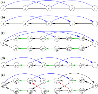
Figure 1: Augmenting a Hamiltonian $st$-path to two edge/internally disjoint $st$-paths. Black edges have cost $0$, blue and red edges have cost $1$. (a) Problem instance. (b) Reducing Min-Cost $2$-EDP Augmentation to Min-Cost $st$-Path. (c) Levels splitting, assuming that the activation costs of the blue edges in (a) are $1$ at $x,v,y$ and $0$ at $s,t$. (d) Reducing Min-Cost $2$-DP Augmentation to Min-Cost $st$-Path. (e) The reduction of [1].

One can also solve the version when we have ordinary edge costs and require that $P\cup F$ contains $2$ internally disjoint $st$-paths. For that, apply a standard reduction that converts edge connectivity problems into node connectivity ones, as follows

1. After step 1 of Algorithm 1, add the In-Out Splitting step, where here the the cost of each edge $v^{\sf in}v^{\sf out}$ is $0$.

2. Replace every edge $u^{\sf out}v^{\sf in}\notin P$ by the edge $u^{\sf in}v^{\sf out}$.

See Fig. 1(d), where after applying this reduction we switched between the names of $v^{\sf in}v^{\sf out}$, to be consistent with the [1] algorithm.

The algorithm of [1] attempts to combine the later reduction with the Levels Reduction in a sophisticated way. In the case when $G$ has a zero cost Hamiltonian $st$-path $P$, $st\notin E$, $L=\{0,1\}$, $L_{s}=L_{t}=\{0\}$, and $c_{uv}^{u}=1$ for all $e=uv\in E\setminus E(P)$ and $u\in V\setminus\{s,t\}$, the [1] algorithm reduces to the following, see Fig. 1(a,e).

1. Construct an edge-weighted directed graph $D_{P}$ with nodes $s=s_{0}^{\sf out},t=t_{0}^{\sf in}$ and $4$ nodes $\{v_{0}^{\sf in},v_{0}^{\sf out},v_{1}^{\sf in},v_{1}^{\sf out}\}$ for every $v\in V\setminus\{s,t\}$. The edge of $D_{P}$ and their weights are:

   1. For $v\in V\setminus\{s,t\}$:                          $w(v_{a}^{\sf out}v_{a}^{\sf in})=0$    $a\in\{0,1\}$.

   2. For $uv\in P$:                                  $w(v_{b}^{\sf in}u_{a}^{\sf out})=a$    $a,b\in\{0,1\}$.
      For $uv\notin P$:                                  $w(u_{a}^{\sf out}v_{b}^{\sf in})=b$    $a,b\in\{0,1\}$, $u_{a}v_{b}\in E$.

2. Compute a cheapest $st$-path $P^{\prime}$ in $D_{P}$ and return the subset of $E$ that corresponds to $P^{\prime}$.

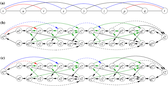
Figure 2: Illustration to the [1] Algorithm. Black edges have weight/thresholds $0$. (a) The input graph; colored edges have thresholds $0$ at $s,t$ and $1$ otherwise. (b) The edge weighted directed graph $D_{P},w$ constructed in the AE reduction and the path (shown by dashed lines) in $D_{P}$ of weight $4$ that corresponds to the optimal solution $\{sx,xz,zt,uy,yq\}$. (c) The path (shown by dashed lines) in $D_{P}$ of weight $4$ that corresponds to the solution $\{sv,uy,xz,yq,pt\}$.

Here for $e=uv\in E$ we write $u_{a}v_{b}\in E$ meaning that $c_{e}^{a}\leq a$ and $c_{e}^{b}\leq b$, namely, that $uv$ can be activated by assigning $a$ units to $u$ and $b$ units to $v$. In the example in Fig. 1(d), the weight of $P^{\prime}$ is $2$ while the optimal solution value is $3$. Still, in this example the [1] algorithm computes an optimal solution. We give a more complicated example, which shows that the approximation ratio of this algorithm is no better than $2$. Consider the graph in Fig. 2(a), with the initial $st$-path

$$s-u-v-x-y-z-p-q-t\ .$$

The optimal solution $\{sx,xz,zt,,uy,yq\}$ (the blue edges and the $uy,yq$ edges) has value $2$ (level assignment $l_{x}=l_{z}=1$ and $0$ otherwise); the $s_{0}^{\sf out}t_{0}^{\sf in}$-path in $D_{P}$ of weight $4$ that corresponds to this solution is (see Fig. 2(b)):

$$s_{0}^{\sf out}{\color[rgb]{0,0,1}\rightarrow}\ x_{1}^{\sf in}\rightarrow v_{0}^{\sf out}\rightarrow v_{0}^{\sf in}\rightarrow u_{0}^{\sf out}\rightarrow y_{0}^{\sf in}{\color[rgb]{0.5,0.5,0}\rightarrow}\ x_{1}^{\sf out}{\color[rgb]{0,0,1}\rightarrow}\ z_{1}^{\sf in}\rightarrow y_{0}^{\sf out}\rightarrow\ q_{0}^{\sf in}\rightarrow p_{0}^{\sf out}\rightarrow p_{0}^{\sf in}{\color[rgb]{0.5,0.5,0}\rightarrow}\ z_{1}^{\sf out}\rightarrow\ t_{0}^{\sf in}\ .$$

The solution $\{sv,uy,xz,yq,pt\}$ (the red edges and the $uy,yq,xz$ edges) has value $4$ (level assignment $l_{v}=l_{x}=l_{z}=l_{p}=1$ and $0$ otherwise); the $s_{0}^{\sf out}t_{0}^{\sf in}$-path in $D_{P}$ of weight $4$ that corresponds to this solution is (see Fig. 2(c)):

$$s_{0}^{\sf out}{\color[rgb]{1,0,0}\rightarrow}\ v_{1}^{in}\rightarrow u_{0}^{\sf out}\rightarrow y_{0}^{\sf in}{\color[rgb]{0.5,0.5,0}\rightarrow}\ x_{1}^{\sf out}{\color[rgb]{0,0,1}\rightarrow}\ z_{1}^{\sf in}\rightarrow y_{0}^{\sf out}\rightarrow q_{0}^{\sf in}{\color[rgb]{0.5,0.5,0}\rightarrow}\ p_{1}^{\sf out}\rightarrow t_{0}^{\sf in}\ .$$

So in $D_{P}$, both paths have the same weight $4$, but one path gives a solution of value $2$ while the other of value $4$.

3 Proof of Theorem 1.3

In this section we will prove Theorem 1.3 – that Activation $2$-DP Augmentation admits a polynomial time algorithm

Recall that for $F\subseteq E$ and $v\in V$ we denote by $\displaystyle\ell_{F}(v)=\max_{e\in\delta_{F}(v)}c_{e}^{v}$ the activation cost incurred by $F$ at $v$, and that for $S\subseteq V$ the activation cost incurred by $F$ at nodes in $S$ is

$$\ell_{F}(S)=\sum_{v\in S}\ell_{F}(v)=\sum_{v\in S}\max_{e\in\delta_{F}(v)}c_{e}^{v}\ .$$

For the proof of Theorem 1.3 it would be convenient to consider a more general problem where each edge $e=uv\in E$ has three costs $c_{e}^{u},c(e),c_{e}^{v}$, where $c_{e}^{u},c_{e}^{v}$ are the activation costs of $e$ and $c(e)$ is the ordinary “middle” cost of $e$. We now describe a method to convert an Activation $2$-DP Augmentation instance into an equivalent instance in which $P$ is a Hamiltonian path but every edge has three costs as above. We call this problem 3-Cost Hamiltonian Activation $2$-DP Augmentation.

Let ${\cal I}=(G=(V,E),c,s,t,P)$ be an Activation $2$-DP Augmentation instance. Let us say that a $uv$-path $Q$ in $G$ is an attachment path if $u,v\in P$ but $Q$ has no internal node in $P$. Note that any inclusion minimal edge set that contains $2$ internally disjoint $st$-paths is a cycle. This implies that if $F$ is an inclusion minimal solution to Activation $2$-DP Augmentation then $\deg_{F}(v)\in\{0,2\}$ for every node $v\in V\setminus V(P)$, hence $F$ partitions into attachment paths. This enables us to apply a prepossessing similar to metric completion, and to construct an equivalent 3-Cost Hamiltonian Activation $2$-DP Augmentation instance $\hat{\cal I}=(\hat{G}=(\hat{V},\hat{E}),\hat{c},s,t,P)$. For this, for every $u,v\in P$ and $(l_{u},l_{v})\in L_{u}\times L_{v}$ do the following.

1. Among all attachment $uv$-paths that have activation costs $l_{u}$ at $u$ and $l_{v}$ at $v$ (if any), compute the cheapest one $Q(l_{u},l_{v})$.

2. If $Q(l_{u},l_{v})$ exists, add a new edge $e=uv$ with activation costs $\hat{c}_{e}^{u}=l_{u},\hat{c}_{e}^{v}=l_{v}$, and ordinary cost $\hat{c}_{e}=\ell_{Q(l_{u},l_{v})}(V)-(l_{u}+l_{v})$ being the activation cost of $Q(l_{u},l_{v})$ on internal nodes of $Q(l_{u},l_{v})$.

After that, remove all nodes in $V\setminus V(P)$. Now $P$ is a Hamiltonian path, and we get a 3-Cost Hamiltonian Activation $2$-DP Augmentation instance $\hat{\cal I}=(\hat{G},\hat{c},s,t,P)$. It is easy to see that the instance $\hat{\cal I}$ can be constructed in polynomial time. Note that the instance ${\cal I}^{\prime}$ may have many parallel edges, but this is allowed, also in the original instance ${\cal I}$.

Now consider some feasible solution $F$ to ${\cal I}$. Replacing every attachment paths contained in $F$ by a single edge as in step 2 above gives a feasible solution $\hat{F}$ to $\hat{\cal I}$ of value at most that of $F$. Conversely, if $\hat{F}$ is a feasible $\hat{\cal I}$ solution, then replacing every edge in $\hat{F}$ by an appropriate path gives a feasible solution $F$ to ${\cal I}$ of value at most that of $\hat{F}$. Consequently, the new instance is equivalent to the original instance in the sense that every feasible solution to one of the instances can be converted to a feasible solution to the other instance of no greater value. We summarize this as follows.

Corollary 3.1.

If 3-Cost Hamiltonian Activation $2$-DP Augmentation admits a polynomial time algorithm then so is Activation $2$-DP Augmentation.

So from now and on our problem is 3-Cost Hamiltonian Activation $2$-DP Augmentation. Let us denote by $\tau(F)$ the sum of the ordinary and the activation cost of $F\subseteq E$, namely

$$\tau(F)=\ell_{F}(V)+c(F)=\sum_{v\in V}\max_{e\in\delta_{F}(v)}c_{e}^{v}+\sum_{e\in F}c(e)\ .$$

Let ${\sf opt}$ denote an optimal solution value for an instance of this problem. We will assume that $V=\{0,1,\ldots,n\}$ and that $P=0-1-\cdots-n$ is a (Hamiltonian) $(0,n)$-path, and view each edge $ij\notin P$ as a directed edge $(i,j)$ where $i<j$. Our goal is to find and edge set $F\subset E$ such that $P\cup F$ contains $2$ internally disjoint $(0,n)$-paths and such that $\tau(F)$ is minimal.

Definition 3.2.

For $0\leq i<j<n$ let ${\cal F}_{i,j}$ denote the family of all edge sets $F\subseteq E$ that satisfy the following two conditions.

1. $F$ is an inclusion minimal edge set such that $P\cup F$ contains $2$ internally disjoint $(j-1,n)$-paths.

2. No edge in $F$ has an end strictly preceding $i$, namely, if $(x,y)\in F$ then $x\geq i$.

We will need the following (essentially known) “recursive” property of the sets in ${\cal F}_{i,j}$.

Lemma 3.3.

$F\in{\cal F}_{i,j}$ if and only if there exists $i\leq x<j$ such that exactly one of the following holds, see Fig. 3(a).

1. $F=\{(x,n)\}$.

2. $F=\{(x,y)\}\cup F^{\prime}$ for some $(x,y)\in E$ with $i\leq x<j<y<n$ and $F^{\prime}\in{\cal F}_{j,y}$.

Proof 3.4.

It is easy to see that if $|F|=1$ then (i) must hold. Assume that $|F|\geq 2$. There is $(x,y)\in F$ with $x<j<y$ as otherwise $(P\cup F)\setminus\{j\}$ has no $(j-1,n)$-path. Let $F^{\prime}=F\setminus\{(x,y)\}$. Then $P\cup F^{\prime}$ contains $2$ internally disjoint $(y-1,n)$-paths, as otherwise $(P\cup F)\setminus\{y\}$ has no $(j-1,n)$-path. Let $x^{\prime}$ be the lowest end of an edge in $F^{\prime}$, let $(x^{\prime},y^{\prime})\in F^{\prime}$, and let $F^{\prime\prime}=F\setminus\{(x^{\prime},y^{\prime})\}$. If $x^{\prime}<j$ then $F^{\prime}\in{\cal F}_{i,j}$ (if $y^{\prime}\geq y$) or $F^{\prime\prime}\in{\cal F}_{i,j}$ (if $y^{\prime}\leq y$), contradicting the minimality of ${\cal F}$. If $x^{\prime}\geq y$ then $(P\cup F)\setminus\{y\}$ has no $(j-1,n)$-path. This implies that $F^{\prime}\in{\cal F}_{i,j}$, hence (ii) holds.

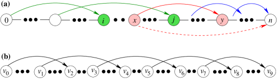
Figure 3: Illustration to Lemma 3.3. Three dots between nodes indicates that these nodes are distinct, while if there are only two dotes then the nodes may coincide.

We note that Lemma 3.3 has the following (essentially known) consequence. Consider an inclusion minimal feasible solution $F$ to our problem. Then the edges in $F$ have an order $(v_{0},v_{2}),(v_{1},v_{4}),(v_{3},v_{6}),\ldots,(v_{2q-1},v_{2q+1})$ such that (see Fig. 3(b))

$$0=v_{0}<v_{1}<v_{2}\leq v_{3}<v_{4}\leq v_{5}<\cdots\leq v_{2q-1}<v_{2q}<v_{2q+1}=n\ .$$

Note that in this node sequence some nodes may be identical (e.g., we may have $v_{2}=v_{3}$), while the others are required to be distinct (e.g., $v_{0}<v_{1}<v_{2}$).

For $(l_{i},l_{j})\in L_{i}\times L_{j}$ let $E(l_{i},l_{j})=\{e\in E:\ell_{e}(l_{i})\leq l_{i},\ell_{e}(l_{j})\leq l_{j}\}$. Let $0\leq i<j<n$. For $F\subseteq E$ the $(l_{i},l_{j})$-forced cost of $F$ is defined by

$$\alpha_{F}(l_{i},l_{j})=\left\{\begin{array}[]{ll}c(F)+\ell_{F}(V\setminus\{i,j\})+l_{i}+l_{j}&\ \mbox{if}\ \ F\subseteq E(l_{i},l_{j})\\ \infty&\mbox{ otherwise}\end{array}\right.$$

Namely, assuming $F\subseteq E(l_{i},l_{j})$ we pay $\ell_{F}(v)$ at every node $v\in V\setminus\{i,j\}$, and in addition we “forcefully” pay $l_{i}$ at $i$ and $l_{j}$ at $j$. Note that

$$\alpha_{F}(l_{i},l_{j})=c(F)+\ell_{F}(V\setminus\{i,j\})+l_{i}+l_{j}=\tau(F)+(l_{i}-\ell_{F}(i))+(l_{j}-\ell_{F}(j))\ .$$

This implies the following.

Corollary 3.5.

$\alpha_{F}(l_{i},l_{j})\geq\tau(F)$ and an equality holds if and only if $\ell_{F}(i)=l_{i}$ and $\ell_{F}(j)=l_{j}$.

Let $f(l_{i},l_{j})$ denote the minimal $(l_{i},l_{j})$-forced cost of an edge set $F\in{\cal F}_{i,j}$, namely

$$f(l_{i},l_{j})=\min_{F\in{\cal F}_{i,j}}\alpha_{F}(l_{i},l_{j})\ .$$ (1)

The number of possible values of $f(l_{i},l_{j})$ is $O(|V|^{2}|L|^{2})$ - there are $O(|V|^{2})$ choices of $i,j$ and at most $|L|^{2}$ choices of $l_{i},l_{j}$. We will show how to compute all these values in polynomial time using dynamic programming. Specifically, we will get a recursive formula that enables to compute each value either directly, or using previously computed values.

The next lemma shows how the function $f(l_{i},l_{j})$ is related to our problem.

Lemma 3.6.

${\sf opt}=\displaystyle{\min_{l_{0},l_{1}\in L}f(l_{0},l_{1})}$.

Proof 3.7.

From the definition of ${\cal F}_{i,j}$ it follows that that ${\cal F}_{0,1}$ is the set of all inclusion minimal feasible solutions. Let $F^{*}$ be an inclusion minimal optimal solution and let $\hat{F}$ be the minimizer of (1). Then for any $l_{0},l_{1}$ we have

$$f(l_{0},l_{1})=\alpha_{\hat{F}}(l_{0},l_{1})\geq\tau(\hat{F})\geq\tau(F^{*})={\sf opt}\ .$$

Consequently, $\displaystyle{\min_{l_{0},l_{1}\in L}f(l_{0},l_{1})}\geq{\sf opt}$. On the other hand for $l_{0}=\ell_{F^{*}}(0)$ and $l_{1}=\ell_{F^{*}}(1)$ we have

$$f(l_{0},l_{1})=\alpha_{F^{*}}(l_{0},l_{1})=\tau(F^{*})={\sf opt}\ ,$$

by Corollary 3.5. This implies $\displaystyle{\min_{l_{0},l_{1}\in L}f(l_{0},l_{1})}\leq{\sf opt}$, concluding the proof.

When $F=\{e\}$ is a single edge we will use the abbreviated notation $\alpha_{e}(l_{i},l_{j})=\alpha_{\{e\}}(l_{i},l_{j})$. For $(l_{i},l_{y})\in L_{i}\times L_{y}$ and an edge $e=(x,y)\in E(l_{i},l_{y})$ with $i\leq x<y$ let $\beta_{e}(l_{i},l_{y})$ be defined by

$$\beta_{e}(l_{i},l_{y})=\left\{\begin{array}[]{ll}0&\mbox{if}\ x=i\\ \ell_{e}(x)&\mbox{if}\ x>i\end{array}\right.$$

We now define two functions that reflect the two different scenarios in Lemma 3.3.

$$g(l_{i},l_{j}) = \min_{e}\{\alpha_{e}(l_{i},l_{j}):e=(x,n)\in E,i\leq x<j\}$$

$$h(l_{i},l_{j}) = \min_{l_{y},e}\{c(e)+l_{i}+\beta_{e}(l_{i},l_{y})+f(l_{j},l_{y}):e=(x,y)\in E(l_{i},l_{y}),i\leq x<j<y\}$$

It is not hard to see that the function $g(l_{i},l_{j})$ is the minimal $(l_{i},l_{j})$-forced cost of a single edge set $e=(x,n)$ such that $\{e\}\in{\cal F}_{i,j}$. Thus if there exist a minimizer of (1) that is a single edge, then $f(l_{i},l_{j})=g(l_{i},l_{j})$.

We will show that the function $h(l_{i},l_{j})$ is the minimal $(l_{i},l_{j})$-forced cost of a non-singleton set $F\in{\cal F}_{i,j}$; note that by lemma 3.3 any such $F$ is a union of some single edge $(x,y)\in F$ with $i\leq x<j<y<n$ and $F^{\prime}\in{\cal F}_{j,y}$. We need the following lemma.

Lemma 3.8.

Let $F\in{\cal F}_{i,j}$ such that $F\subseteq E(l_{i},l_{j})$ and $|F|\geq 2$. Let $(x,y)\in F$ be the first edge of $F$ as in Lemma 3.3, let $F^{\prime}=F\setminus\{e\}$, and let $l_{y}=\ell_{F}(y)$. Then

$$\alpha_{F}(l_{i},l_{j})=c(e)+l_{i}+\beta_{e}(l_{i},l_{y})+\alpha_{F^{\prime}}(l_{j},l_{y})$$

Proof 3.9.

One can verify that for $l_{y}=\ell_{F}(y)$ we have $F^{\prime}\subseteq E(l_{j},l_{y})$ and the following holds:

$$\ell_{F}(V\setminus\{i,j\})=\beta_{e}(l_{i},l_{y})+\ell_{F^{\prime}}(V\setminus\{j,y\})+l_{y}\ .$$

From this and using that $c(F)=c(e)+c(F^{\prime})$ we get

$$\alpha_{F}(l_{i},l_{j}) = c(F)+\ell_{F}(V\setminus\{i,j\})+l_{i}+l_{j}$$

$$= c(e)+l_{i}+\beta_{e}(l_{i},l_{y})+c(F^{\prime})+\ell_{F^{\prime}}(V\setminus\{j,y\})+l_{y}+l_{j}$$

$$= c(e)+l_{i}+\beta_{e}(l_{i},l_{y})+\alpha_{F^{\prime}}(l_{j},l_{y})\ ,$$

as required.

Lemma 3.10.

Among all non-singleton sets in ${\cal F}_{i,j}$ let $F^{*}$ have minimal $(l_{i},l_{j})$-forced cost. Then $h(l_{i},l_{j})=\alpha_{F^{*}}(l_{i},l_{j})$.

Proof 3.11.

We show that $\alpha_{F^{*}}(l_{i},l_{j})\geq h(l_{i},l_{j})$. Let $e=(x,y)\in F^{*}$ be the first edge of $F^{*}$ as in Lemma 3.3(ii), let $F^{\prime}=F\setminus\{e\}$, and let $l_{y}=\ell_{F^{*}}(y)$. Then $e\in E(l_{i},l_{y})$, hence by Lemma 3.8

$$\alpha_{F^{*}}(l_{i},l_{j})=c(e)+l_{i}+\beta_{e}(l_{i},l_{y})+\alpha_{F^{\prime}}(l_{j},l_{y})\geq h(l_{i},l_{j})\ .$$

The inequality is since in the definition of $h(l_{i},l_{j})$ we minimize over $e=(x,y)$ and $l_{y}$.

We show that $\alpha_{F^{*}}(l_{i},l_{j})\leq h(l_{i},l_{j})$. Let $e=(x,y)\in E$ and $l_{y}$ be the parameters for which the minimum in the definition of $h(l_{i},l_{j})$ is attained, and let $F^{\prime}\in{\cal F}_{j,y}$ such that $f(l_{j},l_{y})=\alpha_{F^{\prime}}(l_{j},l_{y})$. Let $F=F^{\prime}\cup\{e\}$ and note that $F\in{\cal F}_{i,j}$ (by Lemma 3.3) and that $l_{y}=\ell_{F}(y)$ (by the definition of $h(l_{i},l_{j})$). Consequently,

$$\alpha_{F^{*}}(l_{i},l_{j})\leq\alpha_{F}(l_{i},l_{j})=c(e)+l_{i}+\beta_{e}(l_{i},l_{y})+f(l_{j},l_{y})=h(l_{i},l_{j})$$

The inequality is since $F^{*}$ has minimal $(l_{i},l_{j})$-forced cost.

We showed that $\alpha_{F^{*}}(l_{i},l_{j})\geq h(l_{i},l_{j})$ and that $\alpha_{F^{*}}(l_{i},l_{j})\leq h(l_{i},l_{j})$, hence the proof is complete.

Let $F^{*}$ be the minimizer of (1). From Lemma 3.10 we have:

• If $|F^{*}|=1$ then $f(l_{i},l_{j})=g(l_{i},l_{j})$.

• If $|F^{*}|\geq 2$ then $f(l_{i},l_{j})=h(l_{i},l_{j})$.

Therefore

$$f(l_{i},l_{j})=\min\{g(l_{i},l_{j}),h(l_{i},l_{j})\}$$ (2)

Note that the quantities $g(l_{i},l_{j})$ can be computed directly in polynomial time. The recurrence in (2) enables to compute values of $f(l_{i},l_{j})$, for all $0\leq i<j\leq n-1$ and $(l_{i},l_{j})\in L_{i}\times L_{j}$, in polynomial time. The number of such values is $O(n^{2}|L|^{2})$, concluding the proof of Theorem 1.3.

Let us illustrate the recursion by showing how the values of $f(l_{i},l_{j})$ are computed for $j=n-1,n-2$. Recall that the values of the function $g$ are computed directly, without recursion and that

$$h(l_{i},l_{j})=\min_{l_{y},e}\{c(e)+l_{i}+\beta_{e}(l_{i},l_{y})+f(l_{j},l_{y}):e=(x,y)\in E(l_{i},l_{y}),i\leq x<j<y\}$$

For $j=n-1$ we have $h(l_{i},l_{j})=\infty$, and thus:

$$f(l_{i},l_{n-1})=g(l_{i},l_{n-1})$$

For $j=n-2$, the only possible value of $y$ is $y=n-1$. For every $i\leq x<y=n-1$ and $e=xy\in E$ we compute directly (without recursion) the values $\beta_{e}(l_{i},l_{y})$. Then

$$\displaystyle h(l_{i},l_{n-2}) = \min_{l_{y},e}\{c(e)+l_{i}+\beta_{e}(l_{i},l_{y})+f(l_{j},l_{y}):e=(x,y)\in E(l_{i},l_{y}),i\leq x<j<y\}$$

$$= \min_{l_{n-1},e}\left\{c(e)+l_{i}+\beta_{e}(l_{i},l_{n-1})+f(l_{n-2},l_{n-1}):\begin{array}[]{ll}e=(x,n-1)\in E(l_{i},l_{n-1})\\ i\leq x<j<n-1\end{array}\right\}$$

Substituting the already computed value $f(l_{n-2},l_{n-1})=g(l_{n-2},l_{n-1})$ enables to compute the minimum of the obtained expression, and thus also to compute $f(l_{i},l_{n}-2)$ via (2).

In a similar way we can compute $h(l_{i},l_{n-3})$, then $f(l_{i},l_{n-3})$, and so on.

References

- [1] H. M. Alqahtani and T. Erlebach. Approximation algorithms for disjoint -paths with minimum activation cost. In CIAC, pages 1–12, 2013.
- [2] H. M. Alqahtani and T. Erlebach. Minimum activation cost node-disjoint paths in graphs with bounded treewidth. In SOFSEM, pages 65–76, 2014.
- [3] E. Althaus, G. Calinescu, I. Mandoiu, S. Prasad, N. Tchervenski, and A. Zelikovsky. Power efficient range assignment for symmetric connectivity in static ad-hoc wireless networks. Wireless Networks, 12(3):287–299, 2006.
- [4] A. Bhaskara, M. Charikar, E. Chlamtac, U. Feige, and A. Vijayaraghavan. Detecting high log-densities: an approximation for densest -subgraph. In STOC, pages 201–210, 2010.
- [5] S. Guha and S. Khuller. Approximation algorithms for connected dominating sets. Algorithmica, 20:374–387, 1998.
- [6] M. Hajiaghayi, G. Kortsarz, V. Mirrokni, and Z. Nutov. Power optimization for connectivity problems. Math. Program., 110(1):195–208, 2007.
- [7] L. M. Kirousis, E. Kranakis, D. Krizanc, and A. Pelc. Power consumption in packet radio networks. Theoretical Computer Science, 243(1-2):289–305, 2000.
- [8] P. Klein and R. Ravi. A nearly best-possible approximation algorithm for node-weighted Steiner trees. J. Algorithms, 19(1):104–115, 1995.
- [9] G. Kortsarz, Z. Nutov, and E. Shalom. Approximating activation edge-cover and facility location problems. Theoretical Computer Science, 930:218–228, 2022.
- [10] Y. Lando and Z. Nutov. On minimum power connectivity problems. J. Discrete Algorithms, 8(2):164–173, 2010.
- [11] P. Manurangsi. Almost-polynomial ratio ETH-hardness of approximating densest -subgraph. In STOC, pages 954–961, 2017.
- [12] Z. Nutov. Approximating minimum power covers of intersecting families and directed edge-connectivity problems. Theoretical Computer Science, 411(26-28):2502–2512, 2010.
- [13] Z. Nutov. Approximating steiner networks with node-weights. SIAM J. Comput., 39(7):3001–3022, 2010.
- [14] Z. Nutov. Activation network design problems. In T. F. Gonzalez, editor, Handbook on Approximation Algorithms and Metaheuristics, Second Edition, volume 2, chapter 15. Chapman & Hall/CRC, 2018.
- [15] Z. Nutov. An -approximation algorithm for minimum power edge disjoint -paths. CoRR, abs/2208.09373, 2022. To appear in CIE 2023. URL: https://doi.org/10.48550/arXiv.2208.09373.
- [16] D. Panigrahi. Survivable network design problems in wireless networks. In SODA, pages 1014–1027, 2011.
- [17] V. Rodoplu and T. H. Meng. Minimum energy mobile wireless networks. In IEEE International Conference on Communications (ICC), pages 1633–1639, 1998.
- [18] A. Segev. The node-weighted Steiner tree problem. Networks, 17:1–17, 1987.
- [19] S. Singh, C. S. Raghavendra, and J. Stepanek. Power-aware broadcasting in mobile ad hoc networks. In Proceedings of IEEE PIMRC, 1999.
- [20] A. Srinivas and E. H. Modiano. Finding minimum energy disjoint paths in wireless ad-hoc networks. Wireless Networks, 11(4):401–417, 2005.
- [21] J E. Wieselthier, G. D. Nguyen, and A. Ephremides. On the construction of energy-efficient broadcast and multicast trees in wireless networks. In Proc. IEEE INFOCOM, pages 585–594, 2000.