Identification Robust Inference for the Risk Premium in Term Structure Models

Abstract

We propose identification robust statistics for testing hypotheses on the risk premia in dynamic affine term structure models. We do so using the moment equation specification proposed for these models in Adrian et al. (2013). We extend the subset (factor) Anderson-Rubin test from Guggenberger et al. (2012) to models with multiple dynamic factors and time-varying risk prices. Unlike projection based tests, it provides a computationally tractable manner to conduct identification robust tests on a larger number of parameters. We analyze the potential identification issues arising in empirical studies. Statistical inference based on the three-stage estimator from Adrian et al. (2013) requires knowledge of the factors’ quality and is misleading without full-rank $\beta$’s or with sampling errors of comparable size as the loadings. Empirical applications show that some factors, though potentially weak, may drive the time variation of risk prices, and weak identification issues are more prominent in multi-factor models.

JEL Classification: C12, C58, G10, G12

Keywords: asset pricing; risk premia; robust inference; weak identification

1 Introduction

A variety of Dynamic affine term structure models (DATSMs) have been developed since the foundational work by Vasicek (1977) and Cox et al. (1985). They help to understand the movements of bond yields and to analyze financial markets. DATSMs are empirically appealing for their smooth tractability and simple characterization of how risks get priced. There are many studies employing this framework. To list a few: Cochrane and Piazzesi (2005) apply affine term structure models to study time variation in expected excess bond returns using a single powerful explanatory factor; Wu and Xia (2016) use affine models to summarize the macroeconomic effects of unconventional monetary policy; Ang and Piazzesi (2003) investigate how macro economic variables affect bond prices and the dynamics of the yield curve, Buraschi and Jiltsov (2005) study the properties of the nominal and real risk premia of the term structure of interest rates and Goliński and Zaffaroni (2016) incorporate long memory state variables into the term structure model. We adopt the DATSMs setup developed by Adrian et al. (2013) which nests a general class of linear asset pricing models and can be regarded as a linear asset pricing model with time-varying risk premia and dynamic factors.

Many recent studies have developed approaches to estimate DATSMs. Most of them involve a time-consuming numerical optimization procedure which results from the high non-linearity. The inference concerning the coefficients suffers similar challenges. Another undesirable feature, as pointed out by, e.g., Hamilton and Wu (2012), is that the identification can be problematic. Lack of identification, e.g., due to unspanned factors (Adrian et al. (2013)), and thus a relatively flat surface of the likelihood also leads to unsatisfying inference results (e.g., Kan and Zhang (1999), Gospodinov et al. (2017), Kleibergen (2009), Hamilton and Wu (2012), Dovonon and Renault (2013), Beaulieu et al. (2016), Khalaf and Schaller (2016), Cattaneo et al. (2022)).

Unspanned factors refer to those that only affect the dynamics of bond prices under the historical measure but not the risk neutral one (see, e.g., Joslin et al. (2014)). The presence of such factors has been documented in empirical studies (e.g., Ludvigson and Ng (2009), Adrian et al. (2013)). They can lead to identification challenges since varying the parameters of the risk neutral pricing measure - risk premia parameters - associated with these factors does not strongly influence bond prices. Adrian et al. (2013) allow for the presence of unspanned factors with the prior knowledge of knowing which factors are unspanned. Their proposed estimation procedure differs for cases with and without unspanned factors.

Because of the identification issues, traditional inference methods based on t-tests and Wald statistics become unreliable for conducting inference on the risk prices in DATSMs (e.g., Stock and Wright (2000) Kleibergen (2005), Antoine and Renault (2020), Andrews and Cheng (2012), Antoine and Lavergne (2022)). We therefore propose easy-to-implement identification robust test procedures which are valid even when the model is not identified due to unspanned factors. The test procedures we provide can be used to study the time-varying risk-premia for linear asset pricing models. Our proposed inference procedures use the framework presented in Adrian et al. (2013), where the risk of bond prices is modeled as a linear functional in observed factors. The risk of bond prices can then be decomposed into two parts: a time-constant and a time-varying part. We propose statistics for testing hypothezes specified on all parameters of the time-varying components and on just subsets of them.

The paper is organized as follows: Section 2 introduces the DATSM. Section 3 states the three step estimation procedure from Adrian et al. (2013) and shows that it is sensitive to identification issues. Section 3 also shows the empirical relevance of these identification issues using the data from Adrian et al. (2013). Section 4 introduces the identification robust tests for the time-varying risk premia. It conducts a small simulation experiment and applies then for an one time-varying risk factor setting. Section 6 introduces the identification robust tests for testing hypothezes on subsets of the time-varying risk premia. It applies them to a variety of multi-factor settings using the data from Adrian et al. (2013). The final sixth section concludes.

We use the following notation throughout the paper: $\otimes\$and vec$(\cdot)$ represent respectively the Kronecker product and vectorization operator; $\Sigma^{\frac{1}{2}}$ is the lower triangular Cholesky decomposition of the positive definite symmetric matrix $\Sigma$ such that $\Sigma=\Sigma^{\frac{1}{2}}\Sigma^{\frac{1}{2}^{\prime}}$; for a $N\times K$ dimensional full rank matrix $A:P_{A}=A(A^{\prime}A)^{-1}A^{\prime}$ and $M_{A}=I_{N}-P_{A}\text{.}$

2 Dynamic affine term structure models (DATSMs)

We briefly discuss the popular class of DATSMs with observed factors. Instead of working directly with the implied yields on an $n$-period bond as usually done in the term structure literature, we make use of the excess holding return of an $n$-period bond as in Adrian et al. (2013).

We first illustrate the model set-up following Adrian et al. (2013) and thereafter consider tests associated with the risk premia. For $P_{t,n}$ the price at time $t$ of a zero-coupon bond maturing at time $t+n\text{,}$ the pricing kernel, $M_{t+1},$ is such that

$$P_{t,n}=E_{t}(M_{t+1}P_{t+1,n-1})\text{.}$$

For $r_{t}$ the one-period short rate and $\lambda_{t}$ the market price of risk, the pricing kernel is assumed exponential affine in innovation factors $v_{t}\sim_{i.i.d}N(0,\Sigma_{v}):$

$$M_{t+1}=\exp\left(-r_{t}-\frac{1}{2}\lambda_{t}^{\prime}\lambda_{t}-\lambda_{t}^{\prime}\Sigma_{v}^{-\frac{1}{2}}v_{t+1}\right),$$

where the market price of risk $\lambda_{t}$ is an affine function of the observed factors $X_{t}:$

$$\lambda_{t}=\Sigma_{v}^{-\frac{1}{2}}\left(\lambda_{0}+\Lambda_{1}X_{t}\right),$$

with $\lambda_{0}$ and $\Lambda_{1}$ resp. a $K$-dimensional vector and a $K\times K$ dimensional matrix, and the $K$-dimensional vector of state variables $X_{t}$ results from a VAR(1):

$$X_{t+1}=\mu+\Phi_{1}X_{t}+v_{t+1}\text{.}$$

For the one-period (log) excess holding return of a $n$-period bond at $t+1:$

$$r_{t+1,n}=\ln\left(P_{t+1,n}\right)-\ln\left(P_{t,n+1}\right)-r_{t}\text{,}$$

with $r_{t}=\ln P_{t,1}$, the structure of the pricing kernel implies that:

$$E_{t}\left[\exp\left(-r_{t+1,n}-\frac{1}{2}\lambda_{t}^{\prime}\lambda_{t}-\lambda_{t}^{\prime}\Sigma_{v}^{-\frac{1}{2}}v_{t+1}\right)\right]=1.$$

Assuming that $(r_{t+1,n}\text{,}$ $v_{t+1})$ are jointly normal, Adrian et al. (2013) show that:

$$E_{t}\left(r_{t+1,n}\right)=\beta^{(n)\prime}\left(\lambda_{0}+\Lambda_{1}X_{t}\right)-\frac{1}{2}var(r_{t+1,n})\text{,}$$

with $\beta^{(n)}=\Sigma_{v}^{-1}cov(v_{t+1},r_{t+1,n})\text{.}$ When decomposing, $R_{t+1,n}$ into a component correlated with $v_{t+1}$ and an uncorrelated component/prediction error $e_{t+1,n}:$

$$\begin{array}[]{c}r_{t+1,n}-E_{t}\left(r_{t+1,n}\right)=\beta^{(n)\prime}v_{t+1}+e_{t+1,n};\end{array}$$

so

$$\begin{array}[]{c}r_{t+1,n}=\beta^{(n)\prime}\left(\lambda_{0}+\Lambda_{1}X_{t}\right)+g^{(n)}(\beta,\Sigma_{v},\Sigma_{e})+\beta^{(n)\prime}v_{t+1}+e_{t+1,n}\text{,}\end{array}$$

where $g^{(n)}(\beta,\Sigma_{v},\Sigma_{e})=-\frac{1}{2}var(r_{t+1,n})\text{,}$ thus, for example, in case $\Sigma_{e}=$var($e_{t+1,n})=\sigma_{e}^{2}\text{,}$ $g^{(n)}(\beta,\Sigma_{v},\Sigma_{e})=-\frac{1}{2}\left(\beta^{(n)\prime}\Sigma_{v}\beta^{(n)}+\sigma_{e}^{2}\right)\text{. }$Additional restrictions are often imposed on the parameters because of the cross-sectional term structure, but these restrictions are dropped in Adrian et al. (2013)’s approach. Assumption 2.1 summarizes the model setting.

Assumption 2.1.

(a) Consider a $K\times 1$ vector of factors $X_{t},$ $t=0,\cdots,T$ that results from a stationary vector autoregression of order 1:

$$\begin{array}[]{c}X_{t+1}=\mu+\Phi_{1}X_{t}+v_{t+1},\end{array}$$

where $v_{t}$ are the innovation shocks (or innovation factors). The log excess holding return $r_{t+1,n-1}$ satisfies:

$${\small\begin{array}[]{c}r_{t+1,n-1}=\beta^{(n-1)^{\prime}}\left(\lambda_{0}+\Lambda_{1}X_{t}\right)+g^{(n-1)}\left(\beta,\Sigma_{v},\Sigma_{e}\right)+\beta^{(n-1)^{\prime}}v_{t+1}+e_{t+1,n-1}\end{array}}$$

with $g^{(n-1)}(\cdot)$ a parametric function. Furthermore:

$$(v_{t+1}^{\prime},e_{t+1}^{\prime})^{\prime}|\left\{X_{s}\right\}_{s=0}^{t}\sim i.i.d.N\left(0,\text{diag}(\Sigma_{v},\Sigma_{e})\right).$$

(b) For $\Sigma_{e}=\sigma_{e}^{2},$ $g^{(n-1)}\left(\beta,\Sigma_{v},\Sigma_{e}\right)=\frac{1}{2}\left(\beta^{(n-1)^{\prime}}\Sigma_{v}\beta^{(n-1)}+\sigma_{e}^{2}\right)$.

3 Regression estimator and Wald based inference

To estimate the price of risk, Adrian et al. (2013) propose a three-step procedure akin to the two pass procedure from Fama and MacBeth (1973):

1. Estimate:

   $$X_{t+1}=\mu+\Phi_{1}X_{t}+v_{t+1}\text{,}$$

   by least squares to obtain $\hat{\mu}\text{,}$ $\hat{\Phi}\text{,}$ $\hat{v}_{t}=X_{t}-\hat{\mu}-\hat{\Phi}_{1}X_{t-1}\text{,}$ $t=1,\ldots,T$ and $\hat{\Sigma}_{v}=\frac{1}{T}\sum_{t=1}^{T}\hat{v}_{t}\hat{v}_{t}^{\prime}\text{.}$

2. Estimate:

   $$r_{t+1,n}=a^{(n)}+d^{(n)\prime}X_{t}+\beta^{(n)\prime}\hat{v}_{t+1}+e_{t+1,n}\text{,}$$

   by least squares to obtain $\hat{a}^{(n)}\text{,}$ $\hat{d}^{(n)}$ and $\hat{\beta}^{(n)}\text{,}$ $n=1,\ldots,N\text{.}$

3. Construct $\hat{a}=(\hat{a}^{(1)}\ldots\hat{a}^{(N)})^{\prime},\text{ }$ $\hat{\beta}=(\hat{\beta}^{(1)}\ldots$ $\hat{\beta}^{(N)})^{\prime},$ $\hat{d}=(\hat{d}^{(1)}\ldots d^{(n)})^{\prime},$ $\hat{g}=(\hat{g}^{(1)}\ldots\hat{g}^{(n)})$ for $\hat{g}^{(n)}=g^{(n)}(\hat{\beta},\hat{\Sigma}_{v},\hat{\Sigma}_{e}),$ $n=1,\ldots,N\text{,}$ and estimate $\lambda_{0}$ and $\Lambda_{1}$ using:

   $$\begin{array}[]{cl}\hat{\lambda}_{0}=&\left(\hat{\beta}^{\prime}\hat{\beta}\right)^{{}^{\prime}-1}\hat{\beta}^{\prime}(\hat{a}+\hat{g}+\hat{\beta}\hat{\mu})\\ \hat{\Lambda}_{1}=&\left(\hat{\beta}^{\prime}\hat{\beta}\right)^{{}^{\prime}-1}\hat{\beta}^{\prime}(\hat{d}+\hat{\beta}\hat{\Phi}).\end{array}$$

The three-step procedure essentially regresses transformed returns on estimated $\beta$’s. Two issues can hamper the reliability of the final stage: the sampling error of estimates resulting from previous stages and the quality of the $\beta$’s. The first issue is negligible when the information dominates the asymptotically vanishing sampling errors, and only slight modifications are necessary for the asymptotic variance estimator used in test statistics to accommodate for it. However, when modeling the unspanned factors, Adrian et al. (2013) show that the entries in the $\beta$’s corresponding to unspanned factors are zero (Assumption 3.1), which leads to identification problems (e.g., Kleibergen (2009), Beaulieu et al. (2013),Kleibergen and Zhan (2015)).

Assumption 3.1.

Potential existence of (nearly) unspanned factors: $\beta^{\prime}=(B,C)$, $B$ represents the spanned factors and is of full rank $K_{B}\leq K$ while $C=O(1/\sqrt{T})$ reflects the (nearly) unspanned factors. If $K_{B}=K,$ there are no (nearly) unspanned factors.

Adrian et al. (2013) show that Assumption 3.1 embeds the unspanned factors that do not affect the dynamics of bonds under the historical pricing measure. The rows of $\beta$ comprised of close to zero values correspond to unspanned factors. Adrian et al. (2013) assume that the location of these rows is known, and their three-step estimation procedure excludes the unspanned factors in the second step by only including spanned factors. The third step would otherwise encounter identification issues resulting from a classical multicollinearity problem. It is straightforward to show that zero $\beta$’s lead to an identification problem because any value of the $\lambda$’s associated with the zero elements in $\beta$ goes for the values of excess returns. When we instead just have small $\beta$’s, which are comparable in magnitude to the estimation error, we similarly encounter such an identification problem (e.g., Kleibergen (2009), Antoine and Renault (2009, 2012), Kleibergen and Zhan (2020), Kleibergen et al. (2022)).

Proposition 3.1 states some well-known results from the weak identification literature. It shows that the risk premia estimator $\hat{\Lambda}$ becomes inconsistent in the presence of weak factors because it converges to a non-normal distribution. This results since varying the value of the risk premia associated with the weak factors does not change the excess returns. The asymptotic distribution of the conventional Wald statistic for testing the null hypothesis $H_{0}:\Lambda_{1}=\Lambda_{1}^{0}$ then no longer converges to a $\chi^{2}$ -distribution, and the same holds for subset testing based on this estimator. Therefore, the conventional test statistics can be misleading in the presence of unspanned factors.

Proposition 3.1.

Under Assumptions 2.1.(a), denote $\Lambda=[\lambda_{0},\Lambda_{1}]$:
(a) If $\beta$ is of full rank:

$$\begin{array}[]{c}\sqrt{T}\left[\begin{matrix}\text{vec}\left(\hat{\beta}^{\prime}-\beta^{\prime}\right)\\ \text{vec}\left(\hat{\Lambda}-\Lambda\right)\end{matrix}\right]\rightarrow_{d}N\left(\left[\begin{matrix}0\\ 0\end{matrix}\right],\left[\begin{matrix}\mathcal{V}_{\beta}&\mathcal{C}_{\Lambda,\beta}^{\prime}\\ \mathcal{C}_{\Lambda,\beta}&\mathcal{V}_{\Lambda}\end{matrix}\right]\right),\end{array}$$

where $\mathcal{V}_{\beta},\mathcal{C}_{\Lambda,\beta},\mathcal{V}_{\Lambda}$ are specified in the proof.
(b) If Assumption 3.1 holds with $K_{B}<K$, then $\hat{\Lambda}\rightarrow_{d}\Lambda+\epsilon,$ where $\epsilon$ follows a non-standard distribution, so $\hat{\Lambda}$ no longer converges to the true value $\Lambda$ at rate $\sqrt{T}$.

Proof.

See the Online Supplementary Appendix. ∎

We focus on inference concerning the time-varying component of risk prices $\Lambda_{1}$. We therefore demean the one-period (log) excess holding returns by subtracting its time-series average:

$$\bar{r}_{t+1,n}=\beta^{(n)\prime}\left(\Lambda_{1}\bar{X}_{t}\right)+\beta^{(n)\prime}\bar{v}_{t+1}+\bar{e}_{t+1,n}\text{,}$$

with $\bar{z}_{t+1,n}=z_{t+1,n}-\bar{z},$ with $\bar{z}=\frac{1}{T}\sum_{t=1}^{T}z_{t},$ for $z=r,$ $X,$ $v$ and $e$ resp. When stacking the equations for $N$ different maturities:

$$R_{t+1}=\beta\left(\Lambda_{1}\bar{X}_{t}\right)+\beta\bar{v}_{t+1}+e_{t+1}\text{,}$$

where $R_{t+1}=(\bar{r}_{t+1,1}\ldots\bar{r}_{t+1,N})^{\prime}\text{,}$ $\beta=(\beta^{(1)}\ldots\beta^{(n)})^{\prime}\text{,}$ $e_{t}=(\bar{e}_{t,1}\ldots\bar{e}_{t,N})^{\prime}\text{,}$ the pricing equation closely resembles the beta-pricing model for the return on (portfolios of) assets:

$$\text{r}_{t+1}=\beta\lambda+\beta\text{F}_{t+1}+u_{t+1}\text{,}$$

with r_t an $N$-dimensional vector with the returns on $N$ assets, $\beta$ the $N\times K$ dimensional beta matrix and $F_{t}$ a $K$ -dimensional vector of risk factors. A further important similarity that both models imply is the reduced rank structure that becomes obvious using a slight re-specification:

$$\begin{array}[]{ccc}R_{t+1}=\beta\left(\Lambda_{1}\ \text{{}}\vdots\ \text{{}}I_{K}\right)\left(\begin{array}[]{c}\bar{X}_{t}\\ \bar{v}_{t+1}\end{array}\right)+e_{t}&&\end{array}$$

and

$$\begin{array}[]{ccc}\text{r}_{t+1}=\beta\left(\lambda\ \text{{}}\vdots\ \text{{}}I_{K}\right)\left(\begin{array}[]{c}1\\ F_{t+1}\end{array}\right)+u_{t},&&\end{array}$$

where the $N\times 2K$ and $N\times(K+1)$ dimensional matrices $\beta(\Lambda_{1}\ \text{{}}\vdots\ \text{{}}I_{K})$ and $\beta(\lambda\ \text{{}}\vdots\ \text{{}}I_{K})$ are each at most of rank $K\text{,}$ so except for the largest $K$ singular values, all, $K$ and 1 resp., singular values of these matrices are zero. Further for $\Lambda_{1}$ and $\lambda$ to be well defined, $\beta$ should be of full rank. When $\beta$ is near a reduced rank value, or in other words, if some factors are weak/unspanned, we encounter an identification issue which is also reflected by more than just $K$ or 1 resp. singular values of the above matrices being equal or close to zero.

	$\hat{\beta}_{1}$	$\hat{\beta}_{2}$	$\hat{\beta}_{3}$	$\hat{\beta}_{4}$	$\hat{\beta}_{5}$
(1)	-0.0094	0.0031	-0.0008	0.0002	0.0000
	(-3.6027)	(2.5058)	(-1.4886)	(0.4344)	(0.0347)
(2)	-0.0213	0.0057	-0.0007	-0.0003	0.0002
	(-8.2107)	(4.5416)	(-1.2228)	(-0.7341)	(0.5816)
(3)	-0.0446	0.0070	0.0010	-0.0005	-0.0001
	(-17.1745)	(5.6040)	(1.8889)	(-1.3535)	(-0.4551)
(4)	-0.0656	0.0048	0.0024	0.0000	-0.0003
	(-25.2648)	(3.8500)	(4.5279)	(0.0386)	(-0.9643)
(5)	-0.0843	0.0003	0.0028	0.0007	-0.0001
	(-32.4670)	(0.2023)	(5.2857)	(1.7192)	(-0.1732)
(6)	-0.1011	-0.0059	0.0022	0.0010	0.0003
	(-38.9474)	(-4.6910)	(4.1584)	(2.6824)	(1.0713)
(7)	-0.1164	-0.0130	0.0008	0.0010	0.0006
	(-44.8511)	(-10.3464)	(1.5602)	(2.5469)	(1.9102)
(8)	-0.1305	-0.0206	-0.0011	0.0005	0.0005
	(-50.2742)	(-16.4072)	(-2.0105)	(1.2971)	(1.8297)
(9)	-0.1435	-0.0284	-0.0033	-0.0003	0.0002
	(-55.2826)	(-22.6118)	(-6.1006)	(-0.8978)	(0.6354)
(10)	-0.1556	-0.0361	-0.0056	-0.0015	-0.0005
	(-59.9307)	(-28.7667)	(-10.3483)	(-3.7935)	(-1.6457)
(11)	-0.1669	-0.0436	-0.0078	-0.0028	-0.0014
	(-64.2706)	(-34.7284)	(-14.4913)	(-7.1319)	(-4.8558)
	[0.0000]	[0.0000]	[0.0000]	[0.0000]	[0.0001]

Table 1: The least squares estimates of the $\beta$’s associated with the excess returns for bonds with 11 different maturities of $6,12,18\cdots,60$ and 84, 120 months over the sample period 1987:01-2011:12, and the factors are the first five principal components generated using the cross-section of bond yields for maturities $3,\cdots,120$ months (same data taken from Adrain et al. (2013)). Based on Proposition 3.1.(a), we report LS estimates of $\beta$’s with t-statistics in round brackets; and$p$-values of $F$-tests in square brackets, testing the null hypothesis $H_{0}:\beta_{j}=0$ that each column is jointly zero.. The Kleibergen-Paap rank statistic (see Kleibergen and Paap (2006)) testing $H_{0}:$ rank($\beta$)=4: 1.6561 [0.9764].

Illustrating unspanned and weak factors in an empirical study

In reality, there is no direct prior knowledge of the number of unspanned or weak factors. To show their presence and empirical relevance, we use the data from Adrian et al. (2013), i.e., the zero coupon yield data constructed by Gürkaynak et al. (2007). Table 1 shows the factor loading estimates and relevant tests corresponding to the five principal component (PCA) factors employed in Adrian et al. (2013). Table 1 shows that many elements of $\beta$ are small and not statistically significant from zero at the 5% significance level. Though the $F$-tests on the columns of $\beta$ are significant, the rank test of the $\beta$-matrix indicates potential identification problems, because for these factor loadings we can not reject the reduced rank null hypothesis at the 5% significance level.

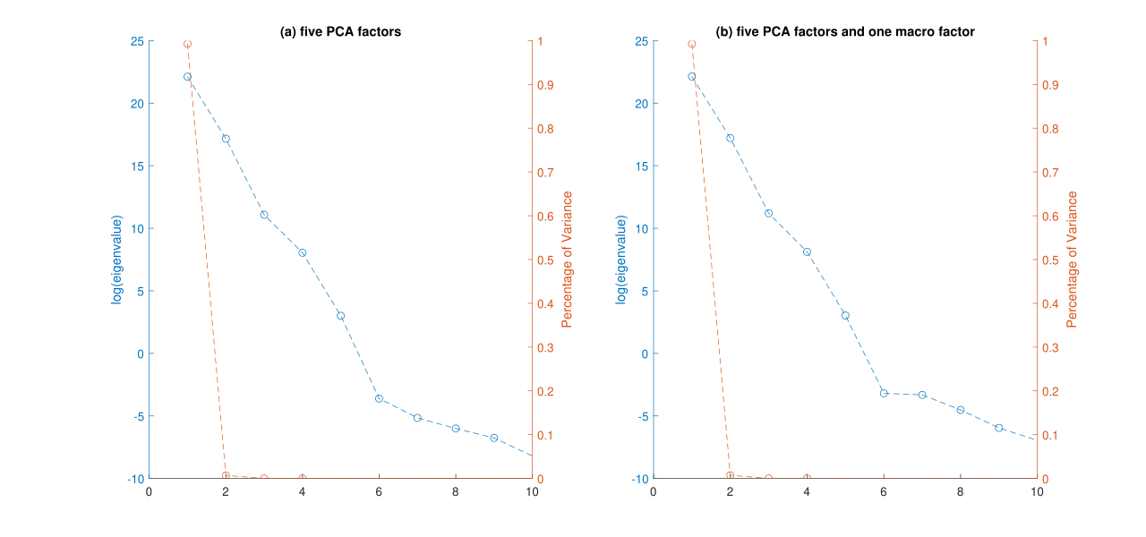
Figure 1: (log) singular values (blue) and the percentage of variance explained (red) of $\displaystyle\frac{1}{T}\sum_{t=1}^{T}R_{t}\left(\begin{array}[]{c}\bar{X}_{t}\\ \hat{v}_{t+1}\end{array}\right)^{\prime}\left[\frac{1}{T}\sum_{t=1}^{T}\left(\begin{array}[]{c}\bar{X}_{t}\\ \hat{v}_{t+1}\end{array}\right)\left(\begin{array}[]{c}\bar{X}_{t}\\ \hat{v}_{t+1}\end{array}\right)^{\prime}\right].$ $R_{t}$ uses the demeaned excess returns of the same bonds as in Table 1, $\bar{X}_{t}$ involves the five PCA factors in (a) and uses the five PCA factors with one additional macro factor in (b).

Figure 1.(a) uses the same data set as Table 1 and shows a scree plot of the (log) singular values of

$$\frac{1}{T}\sum_{t=1}^{T}R_{t}\left(\begin{array}[]{c}\bar{X}_{t}\\ \hat{v}_{t+1}\end{array}\right)^{\prime}\left[\frac{1}{T}\sum_{t=1}^{T}\left(\begin{array}[]{c}\bar{X}_{t}\\ \hat{v}_{t+1}\end{array}\right)\left(\begin{array}[]{c}\bar{X}_{t}\\ \hat{v}_{t+1}\end{array}\right)^{\prime}\right],$$

which estimates $\beta(\Lambda_{1}\ \text{{}}\vdots\ \text{{}}I_{K})$. In case of strong spanned factors, the smallest $K,$ is five, singular values should be close to zero while Figure 1.(a) shows that the smallest six singular values are close to zero which indicates a weak/unspanned factor problem which is further reflected by the rank test not rejecting rank($\beta$)=4 in Table 1 at the 5% significance level.

	$\hat{\beta}_{1}$	$\hat{\beta}_{2}$	$\hat{\beta}_{3}$	$\hat{\beta}_{4}$	$\hat{\beta}_{5}$	$\hat{\beta}_{\mathit{macro}}$
(1)	-0.0094	0.0032	-0.0008	0.0002	0.0000	0.0001
	(-3.4930)	(2.4109)	(-1.4749)	(0.4253)	(0.0309)	(0.0516)
(2)	-0.0213	0.0057	-0.0007	-0.0003	0.0002	0.0000
	(-7.9353)	(4.3501)	(-1.2115)	(-0.7259)	(0.5717)	(0.0254)
(3)	-0.0446	0.0070	0.0010	-0.0005	-0.0001	-0.0000
	(-16.5873)	(5.3631)	(1.8715)	(-1.3372)	(-0.4497)	(-0.0037)
(4)	-0.0656	0.0049	0.0024	0.0000	-0.0003	0.0001
	(-24.4149)	(3.6980)	(4.4871)	(0.0346)	(-0.9529)	(0.0655)
(5)	-0.0843	0.0003	0.0028	0.0007	-0.0001	0.0001
	(-31.3724)	(0.2100)	(5.2383)	(1.6937)	(-0.1732)	(0.0801)
(6)	-0.1011	-0.0059	0.0022	0.0010	0.0003	0.0000
	(-37.6206)	(-4.4799)	(4.1208)	(2.6462)	(1.0539)	(0.0333)
(7)	-0.1164	-0.0130	0.0008	0.0010	0.0006	-0.0000
	(-43.3100)	(-9.8999)	(1.5456)	(2.5142)	(1.8813)	(-0.0252)
(8)	-0.1305	-0.0206	-0.0011	0.0005	0.0005	-0.0001
	(-48.5424)	(-15.7013)	(-1.9930)	(1.2811)	(1.8021)	(-0.0512)
(9)	-0.1435	-0.0284	-0.0033	-0.0003	0.0002	-0.0000
	(-53.3870)	(-21.6288)	(-6.0457)	(-0.8872)	(0.6243)	(-0.0204)
(10)	-0.1557	-0.0361	-0.0056	-0.0015	-0.0005	0.0001
	(-57.8990)	(-27.4937)	(-10.2541)	(-3.7506)	(-1.6271)	(0.0745)
(11)	-0.1670	-0.0435	-0.0078	-0.0028	-0.0014	0.0002
	(-62.1305)	(-33.1560)	(-14.3589)	(-7.0557)	(-4.7981)	(0.2297)
	[0.0000]	[0.0000]	[0.0000]	[0.0000]	[0.0002]	[1.0000]

Table 2: Using the same data as in Table 1 with one additional macro factor (real activity) that constructed following Ang and Piazzesi (2003), we report estimates of the $\beta$’s with t-statistics in round brackets; and $p$-values of $F$-tests in square brackets, testing the null hypothesis $H_{0}:\beta_{j}=0$ that each column is jointly zero. Kleibergen-Paap rank statistic testing $H_{0}:$ rank($\beta$ )=5: 0.0025 [1.0000].

As previously noted in the literature (e.g., Kleibergen and Zhan (2020), Kleibergen et al. (2022)), weak identification issues are often present when macro factors are used. Following Ang and Piazzesi (2003), we construct one macro factor, the real activity measure, which is the first principal component resulting from four variables that capture real US macro activity: the ”Help Wanted Advertising in Newspapers (HELP)” index, unemployment (UE), the growth rate of employment (EMPLOY), and the growth rate of industrial production (IP). As shown in Table 2, the macro factor is much less correlated with returns and thus is more likely to result in an identification issue. This is further reflected in Figure 1(b) containing the scree plot which shows that while there are six factors, the smallest seven singular values are close to zero. Table 2 also shows a tiny value for the rank test which provides another indication of a weak/unspanned factor problem.

The identification problems revealed in Figures 1-2 and Tables 1-2 not only affect the validity of the estimators but also the reliability of traditional inference procedures. Adrian et al. (2013) assume that the positions of the zero rows in $\beta$ are known when dealing with unspanned factors. We remain agnostic about this and provide testing procedures concerning $\Lambda_{1}$ which are identification robust without the need of prior knowledge of the unspanned factors.

4 Identification robust tests of time-varying risk premia

The identification robust tests are based on the sample moment vector. The sample moment vector results from the observed factors having no predictive power for the prediction error, $\bar{e}_{t+1,n},$ so our sample moment vector for $\Lambda_{1}$ is:

$$\begin{array}[]{c}f_{T}(\Lambda_{1},X)=\frac{1}{T}\sum_{t=1}^{T}(\bar{X}_{t-1}\otimes(\bar{R}_{t}-\hat{\beta}\hat{V}_{t}))-\left(\hat{Q}_{XX}\otimes\hat{\beta}\right)\text{vec(}\Lambda_{1}),\end{array}$$

with $\hat{Q}_{XX}=\frac{1}{T}\sum_{t=1}^{T}\bar{X}_{t-1}\bar{X}_{t-1}^{\prime},$ and its derivative with respect to vec($\Lambda_{1})$ is

$$\begin{array}[]{c}q_{T}(X)=-\left(\hat{Q}_{XX}\otimes\hat{\beta}\right)\text{.}\end{array}$$

We next make an assumption regarding the large sample behavior of the sample moment vector and its derivative.

Assumption 4.1.

Under $H_{0}:\Lambda_{1}=\Lambda_{1}^{0}$,

$$\sqrt{T}\left(\begin{array}[]{c}f_{T}(\Lambda_{1}^{0},X)\\ \text{vec}(q_{T}(X)-J)\end{array}\right)\underset{d}{\rightarrow}\left(\begin{array}[]{c}\psi_{f}\\ \psi_{q}\end{array}\right)\text{,}$$

where the Jacobian $J=-(Q_{XX}\otimes\beta),$ $\hat{Q}_{XX}\underset{p}{\rightarrow}Q_{XX}\text{,}$ and $\psi_{f}$ and $\psi_{q}$ are $N\times K$ and $NK\times K^{2}$ dimensional random vectors:

$$\left(\begin{array}[]{c}\psi_{f}\\ \psi_{q}\end{array}\right)\sim N\left(0,V(\Lambda_{1}^{0})\right)\text{,}$$

with

$$V(\Lambda_{1}^{0})=\left(\begin{array}[]{cc}V_{ff}(\Lambda_{1}^{0})&V_{qf}(\Lambda_{1}^{0})^{\prime}\\ V_{qf}(\Lambda_{1}^{0})&V_{qq}(\Lambda_{1}^{0})\end{array}\right),$$

where $V_{ff}(\Lambda_{1}^{0}),$ $V_{qf}(\Lambda_{1}^{0})$ and $V_{qq}(\Lambda_{1}^{0})$ are $NK\times NK,$ $NK^{3}\times NK$ and $NK^{3}\times NK^{3}$ dimensional matrices.

Assumption 4.1 is a high-level assumption which resembles Assumption 1 in Kleibergen (2005) and holds under mild conditions. Assumption 4.1 holds true irrespective of Assumption 3.1. Assumption 2.1 is sufficient for Assumption 4.1, but our proposed test statistics can be applied to more general cases than the model implied in Assumption 2.1. For our setting:

$$\psi_{f}=\psi_{\bar{f}}+\Psi_{q}\text{vec(}\Lambda_{1}^{0})\text{,}$$

with $\Psi_{q}=$vecinv($\psi_{q})$ and

$$\begin{array}[]{c}\sqrt{T}\left(\frac{1}{T}\sum_{t=1}^{T}(\bar{X}_{t-1}\otimes(\bar{R}_{t}-\hat{\beta}\hat{V}_{t}))-\left(Q_{XX}\otimes\beta\right)\text{vec}(\Lambda_{1}^{0})\right)\underset{d}{\rightarrow}\psi_{\bar{f}}\text{.}\end{array}$$

We also have

$$\psi_{q}=\text{vec}((Q_{XX}\otimes\Psi_{\beta})+(\Psi_{XX}\otimes\beta))\text{,}$$

where

$$\begin{array}[]{cl}\sqrt{T}\text{vech}(\frac{1}{T}\sum_{t=1}^{T}\bar{X}_{t}\bar{X}_{t}^{\prime}-Q_{XX})\underset{d}{\rightarrow}\psi_{XX}\text{,}&\Psi_{XX}=\text{ vechinv}(\psi_{XX})\text{,}\\ \sqrt{T}\text{vec}(\hat{\beta}-\beta)\underset{d}{\rightarrow}\psi_{\beta}\text{ ,}&\Psi_{\beta}=\text{vecinv}(\psi_{\beta})\text{,}\end{array}$$

with vech$(A)$ containing the unique elements of a symmetric matrix $A$. Since $\psi_{q}$ has $NK^{3}$ elements while the number of unique elements in $\Psi_{\beta}$ and $\Psi_{XX}$ equals $NK+\frac{1}{2}K(K+1)\text{,}$ the joint normal distribution of $(\psi_{f}\text{,}$ $\psi_{q})$ is further allowed to be degenerate. When $v_{t}$ is normal (as assumed in Assumption 2.1) or its third moment equals zero, $\psi_{\beta}$ and $\psi_{XX}$ are also independently distributed.

The identification robust statistics use an estimator of the Jacobian whose limit behavior under H${}_{0}:\Lambda_{1}=\Lambda_{1}^{0}$ is independent of the limit behavior of the sample moment, see Kleibergen (2005):

$$\begin{array}[]{rl}\hat{D}_{T}(\Lambda_{1},X)=&(\hat{D}_{1,T}(\Lambda_{1},X)\ldots\hat{D}_{1,T}(\Lambda_{k},X))\\ \text{vec(}\hat{D}_{T}(\Lambda_{1},X))=&\text{vec}(q_{T}(X))-\hat{V}_{qf}(\Lambda_{1})\hat{V}_{ff}(\Lambda_{1})^{-1}f_{T}(\Lambda_{1},X)\\ \sqrt{T}\text{vec(}\hat{D}_{T}(\Lambda_{1}^{0},X)-J)\underset{d}{\rightarrow}&\psi_{q.f}\sim N(0,V_{qq.f}(\Lambda_{1}^{0}))\end{array}$$

with $V_{qq.f}(\Lambda_{1})=V_{qq}-V_{qf}(\Lambda_{1})V_{ff}(\Lambda_{1})^{-1}V_{qf}(\Lambda_{1})^{\prime}\text{,}$ $\hat{V}_{qf}(\Lambda_{1})$ and $\hat{V}_{ff}(\Lambda_{1})$ consistent estimators of $V_{qf}(\Lambda_{1}^{0})$ and $V_{ff}(\Lambda_{1}^{0}),$ and $\psi_{q.f}$ independent of $\psi_{f}.$

We can next define the identification robust Factor Anderson-Rubin (FAR), (Kleibergen) Lagrange multiplier (KLM) and JKLM statistics for testing H${}_{0}:\Lambda_{1}=\Lambda_{1}^{0}:$

$$\begin{array}[]{cl}\text{FAR(}\Lambda_{1}^{0})=&T\times f_{T}(\Lambda_{1}^{0},X)^{\prime}\hat{V}_{ff}(\Lambda_{1}^{0})^{-1}f_{T}(\Lambda_{1}^{0},X)\underset{d}{\rightarrow}\chi^{2}(KN)\\ \text{KLM(}\Lambda_{1}^{0})=&T\times f_{T}(\Lambda_{1}^{0},X)^{\prime}\hat{V}_{ff}(\Lambda_{1}^{0})^{-\frac{1}{2}}P_{\hat{V}_{ff}(\Lambda_{1}^{0})^{-\frac{1}{2}}\hat{D}_{T}(\Lambda_{1}^{0},X)}\\ \text{\thinspace\thinspace}&\text{\quad\quad\quad\quad\quad\quad}\hat{V}_{ff}(\Lambda_{1}^{0})^{-\frac{1}{2}}f_{T}(\Lambda_{1}^{0},X)\underset{d}{\rightarrow}\chi^{2}(K^{2})\\ \text{JKLM(}\Lambda_{1}^{0})=&T\times f_{T}(\Lambda_{1}^{0},X)^{\prime}\hat{V}_{ff}(\Lambda_{1}^{0})^{-\frac{1}{2}}M_{\hat{V}_{ff}(\Lambda_{1}^{0})^{-\frac{1}{2}}\hat{D}_{T}(\Lambda_{1}^{0},X)}\\ \text{\thinspace\thinspace}&\text{\quad\quad\quad\quad\quad\quad}\hat{V}_{ff}(\Lambda_{1}^{0})^{-\frac{1}{2}}f_{T}(\Lambda_{1}^{0},X)\underset{d}{\rightarrow}\chi^{2}(K(N-K)).\end{array}$$

The limiting distributions are a direct result of Assumption 4.1 and do not depend on the rank of the Jacobian or $\beta$, so the limiting distributions hold regardless of Assumption 3.1.

4.1 Illustrative simulation and empirical results

We conduct a single-factor model simulation study to illustrate the performance of the proposed robust joint tests. For the data generating process (DGP), we consider

$$R_{t}=c+\beta\left(\Lambda_{1}X_{t-1}+v_{t}\right)+e_{t}\text{,}$$

where the parameters are calibrated to data from Adrian et al. (2013). In particular, we fix the sample size to be $T=300$ and use the eleven excess returns as in Table 1. We calibrate with the first PCA factor from Adrian et al. (2013) to mimic the strong identified case and the third one for the weak identification setting. Figure 2 shows power curves of the conventional t-statistic and the robust test statistics in both strong and weakly identified cases. For both settings, FAR, KLM and JKLM tests are all size correct, while the Wald test is size distorted under weak identification and size correct but biased for stong identification. For weak identification, the KLM test has some power loss away from the hypothesized value because of which it is preferred to combine it in a conditional or unconditional manner with the J-test to improve power, see Moreira (2003) and Kleibergen (2005).

We use the robust tests to analyze the time-varying component of the risk premium. A detailed description of the involved excess returns and risk factors has been discussed previously for Tables 1-2. Figure 3 shows the $p$-values for testing the risk premium associated with all six factors in a single factor model with the identification robust tests. A $p$-value larger than, say, 5%, implies that we could not reject the null at the 5% significance level.

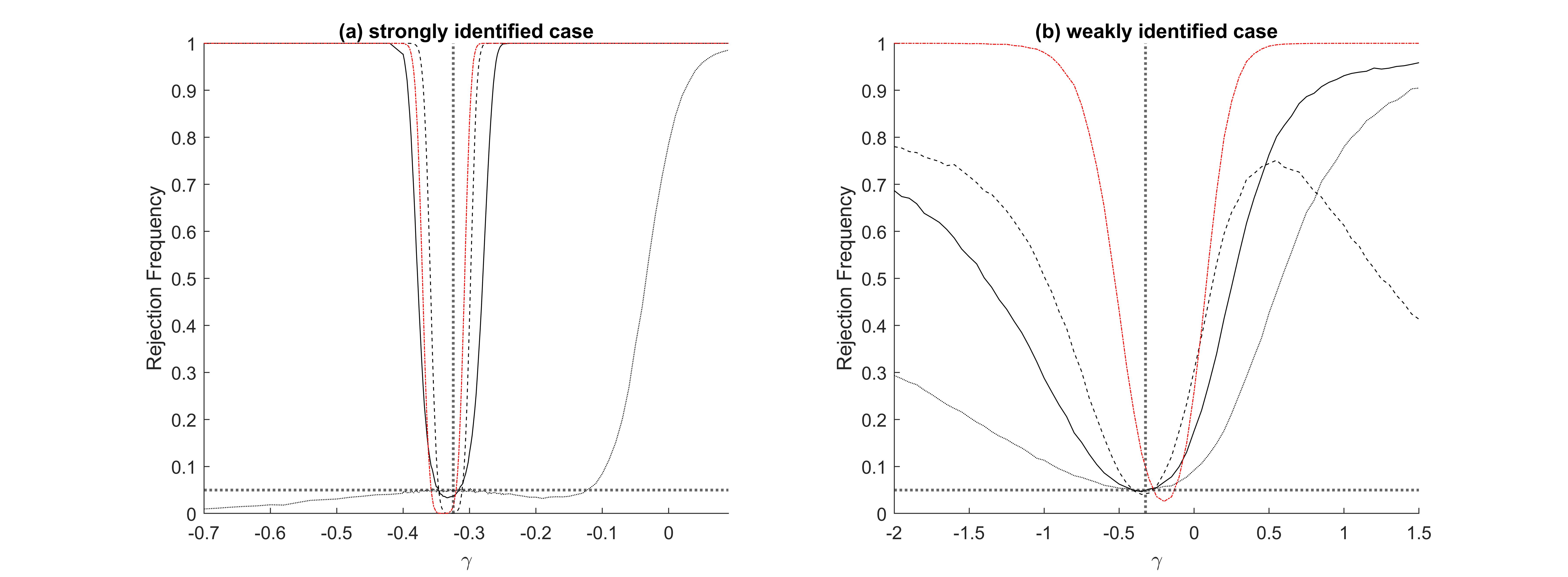
Figure 2: the left panel (a) is the strong identified case, while the right panel (b) is the weak identified case. Power curves (rejection frequencies) of Wald (dash-dotted, red), FAR (solid), KLM (dashed), and JKLM (dotted) testing the $\Lambda_{1}$ (scalar) with values on the horizontal axis; horizontal dashed line at 5% and vertical one at the calibrated value of $\Lambda_{1}$.

Figure 3 shows that for most cases the JKLM test leads to unbounded 95% confidence sets even for strong factors, e.g., the first PCA factor, since the $p$-value curves are above the 5% line over the whole interval of analyzed values of the risk premium which is consistent with the smaller power observed in our simulation exercises and results since the JKLM test primarily tests misspecification. For all factors, the FAR and KLM tests provide bounded 95% confidence sets since only for bounded regions the $p$-values are above the 5% line, even for those potentially weak factors such as the fifth PCA factor and the macro factor. The latter implies that in a single factor setting, all these risk premia are identified. For the high-order PCA factors, the robust tests, however, result in 95% confidence sets that differ from those resulting from the Wald test. Most striking is that a zero value for the risk premium is not rejected for strong factors such as the first and second PCA factors but rejected for potentially weak factors. For example, the null hypothesis that $\Lambda_{1}=0$ is rejected by the FAR and KLM test for both the fifth factor and the macro factor. This is partly in line with Adrian et al. (2013), which highlight the role of the higher-order principal components as the time variation may be largely driven by, e.g., the fifth principal component. Therefore, some factors may be weak but have some importance for interpreting the (time-varying) expected returns.

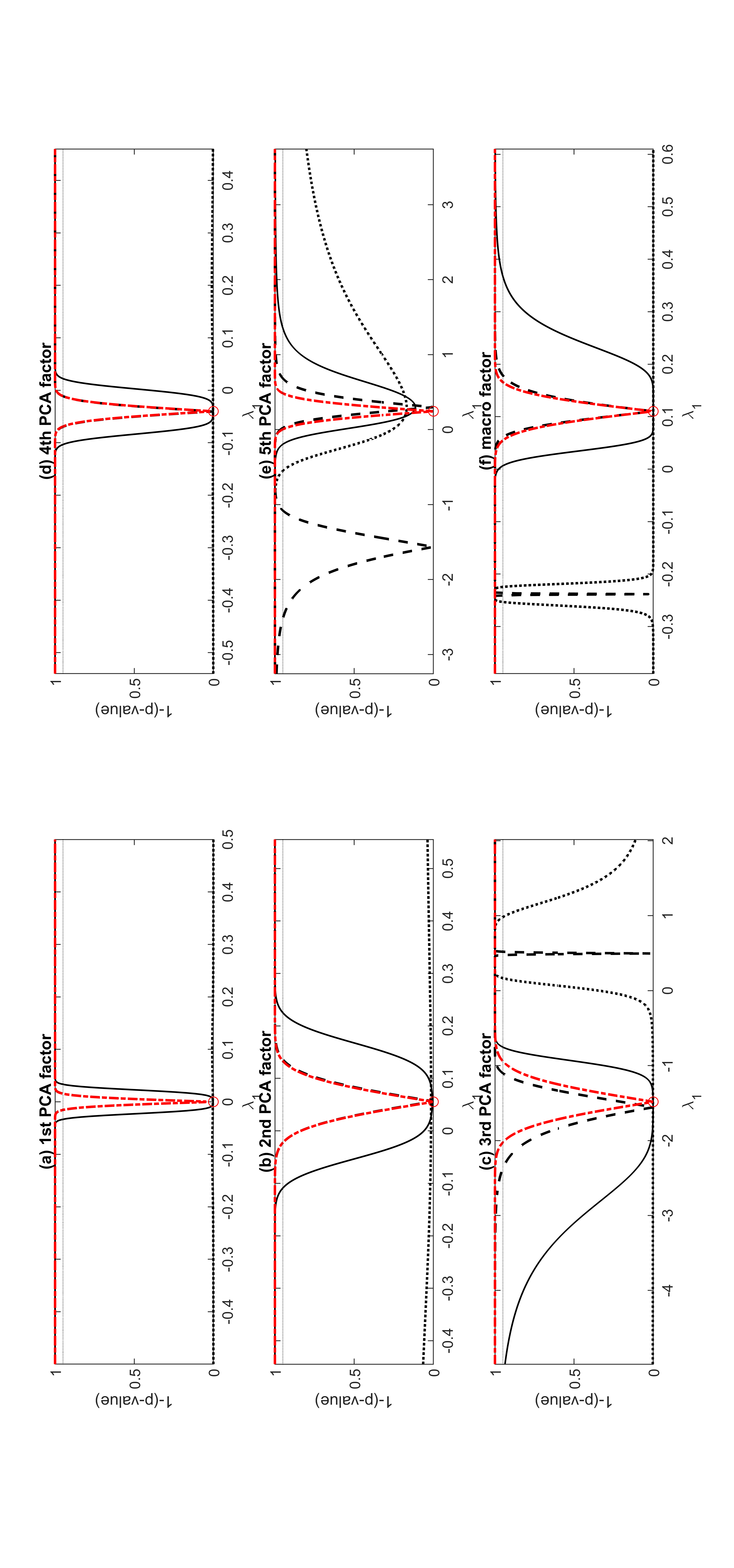
Figure 3: one-minus-$p$-value curves of Wald (dash-dotted, red); FAR (solid); KLM (dashed); JKLM (dotted) for testing the $\Lambda_{1}$ (scalar) in a single factor model with values on the horizontal axis and dotted line at 95%. This figure uses the same data as in Table 2.

5 Identification robust sub-vector testing

The identification robust tests introduced in the previous section are for testing hypotheses specified on all elements of $\Lambda_{1}.$ We are often interested in testing hypotheses specified on just subsets of the parameters. When we analyze multi-factor models, testing whether or not a certain factor risk premium exhibits time variation would require testing a specific row of $\Lambda_{1}$, while testing whether a factor drives the time variation would require to test the corresponding column of $\Lambda_{1}$. Under our current settings, projection-based versions of the identification robust tests would allow us to test such hypotheses whilst preserving the size of the test, see Dufour and Taamouti (2005). These tests, however, lead to reduced power so we extend the robust subset FAR test (sFAR) of Guggenberger et al. (2012) for testing hypotheses on all elements in a row of $\Lambda_{1}$ which can be similarly extended to test for all elements in a column of $\Lambda_{1}$.

Without loss of generality, we consider testing the hypothesis that the risk premia associated with one specific factor, say the first, are all equal to $\lambda_{1}^{0}$:

$$\text{H}_{0}:\lambda_{1}=\lambda_{1}^{0},$$

for $\Lambda_{1}=\binom{\lambda_{1}^{0\prime}}{\Lambda_{2}},$ $\lambda_{1}:K\times 1,$ $\Lambda_{2}:(K-1)\times K.$ Under H${}_{0}:\lambda_{1}=\lambda_{1}^{0},$ the $N\times 2K$ dimensional reduced rank parameter matrix in the equation for the stacked returns becomes:

$$\Phi=\left(\beta_{1}\ \text{{}}\vdots\ \text{{}}\beta_{2}\right)\left(\begin{array}[]{ccc}\lambda_{1}^{0\prime}&1&0\\ \Lambda_{2}&0&I_{K-1}\end{array}\right),$$

so post-multiplying by $\left(\begin{matrix}{I_{K}}&{-\lambda_{1}^{0}}&{0}\\ {0}&0&{I_{K-1}}\end{matrix}\right)^{\prime}$ yields the $N\times(2K-1)$ matrix:

$$\Phi\left(\begin{array}[]{cc}I_{K}&0\\ -\lambda_{1}^{0\prime}&0\\ 0&I_{K-1}\end{array}\right)=\left(\beta_{1}\ \text{{}}\vdots\ \text{{}}\beta_{2}\right)\left(\begin{array}[]{cc}0&0\\ \Lambda_{2}&I_{K-1}\end{array}\right)=\beta_{2}\left(\begin{array}[]{cc}\Lambda_{2}&I_{K-1}\end{array}\right),$$

which, since the rank of $\beta_{2}\left(\begin{array}[]{cc}\Lambda_{2}&I_{K-1}\end{array}\right)$ equals $K-1,$ shows that H₀ implies that the smallest $K$ singular values of $\Phi$ times $\left(\begin{matrix}{I_{K}}&{-\lambda_{1}^{0}}&{0}\\ {0}&0&{I_{K-1}}\end{matrix}\right)^{\prime}$ equal zero. The sFAR statistic for testing H${}_{0}:\lambda_{1}=\lambda_{1}^{0}:$

$$\begin{array}[]{cc}\text{sFAR(}\lambda_{1})=&\min_{\Lambda_{2}}\text{FAR}(\Lambda_{1}(\lambda_{1}^{0},\Lambda_{2})),\end{array}$$

therefore corresponds with a rank test of H${}_{0}:$ rank$\left(\Phi\left(\begin{array}[]{cc}I_{K}&0\\ -\lambda_{1}^{0\prime}&0\\ 0&I_{K-1}\end{array}\right)\right)=K-1.\vskip 12.0pt plus 4.0pt minus 4.0pt$

The bounding distribution of the limiting distribution of the sFAR statistic relies upon a Kronecker product structure (KPS) asymptotic covariance matrix of the least squares estimator of the linear model ( see Guggenberger et al. (2012)):

$$\hat{\Phi}=\frac{1}{T}\sum_{t=1}^{T}R_{t}\left(\begin{array}[]{c}\bar{X}_{t}\\ \hat{v}_{t+1}\end{array}\right)^{\prime}\left[\frac{1}{T}\sum_{t=1}^{T}\left(\begin{array}[]{c}\bar{X}_{t}\\ \hat{v}_{t+1}\end{array}\right)\left(\begin{array}[]{c}\bar{X}_{t}\\ \hat{v}_{t+1}\end{array}\right)^{\prime}\right]^{-1}=\left(\hat{d}\ \text{{}}\vdots\ \text{{}}\hat{\beta}\right).$$

The KPS thus concerns the asymptotic variance of

$$\begin{array}[]{cc}\frac{1}{\sqrt{T}}\sum_{t=1}^{T}\left(\begin{array}[]{c}\bar{X}_{t}\\ \hat{v}_{t+1}\end{array}\right)\otimes\tilde{e}_{t},&\tilde{e}_{t}=e_{t}+\beta(\bar{v}_{t}-\hat{v}_{t}).\end{array}$$

We note that $\hat{v}_{t}$ is not directly observed so it adds additional sampling error when imputing estimates of $\hat{v}_{t}.$ To implement the sFAR test, we therefore make the following assumption.

Assumption 5.1.

There exists $\Omega\in\mathbb{R}^{2K\times 2K}$ and $\Sigma\in\mathbb{R}^{N\times N}$ symmetric positive definite matrices such that $S=\Omega\otimes\Sigma$ and

$$\begin{array}[]{c}\frac{1}{\sqrt{T}}\sum_{t=1}^{T}\left(\left(\begin{array}[]{c}\bar{X}_{t}\\ \hat{v}_{t+1}\end{array}\right)\otimes\tilde{e}_{t}\right)\rightarrow_{d}N(0,S).\end{array}$$

The asymptotic normality stated in Assumption 5.1 is a direct result of Assumption 2.1. If $\hat{v}_{t}$ is directly observed, so $\tilde{e}_{t}=e_{t}$, Assumption 2.1 implies that $\Omega=\mathbb{E}\left((\bar{X}_{t}^{\prime}\text{ }\vdots\text{ }\hat{v}_{t+1}^{\prime})^{\prime}(\bar{X}_{t}^{\prime}\text{ }\vdots\text{ }\hat{v}_{t+1}^{\prime})\right)$ and $\Sigma=\text{var}(e_{t})$. Because of the additional sampling error due to the generated regressor $\hat{v}_{t+1}$, Assumption 5.1 does, however, not provide the exact specifications of $\Omega$ and $\Sigma$.

	(1)	(2)	(3)	(4)
KPST	212.0808	201.8551	197.1613	205.8054
$p$-value	[0.0511]	[ 0.1265]	[ 0.1809]	[0.0910]

Table 3: KPS test (KPST) statistics for testing the null hypothesis that $H_{0}:S=\Omega\otimes\Sigma$ for some $\Omega\in\mathbb{\ \ R}^{2K\times 2K}$ and $\Sigma\in\mathbb{R}^{N\times N}$ symmetric positive definite matrices. All four cases use excess returns on bonds with maturities 3, 12, 24, 60, 90, 120 months from Adrian et al. (2013). For the factors $X_{t}$, (1) uses the macro factor (real activity) and the level factor (first PCA factor), (2) uses the level factor (first PCA factor) and the slope factor (second PCA factor), (3) uses the macro factor (real activity) and the slope factor (second PCA factor) and (4) uses the macro factor (real activity) and the curvature factor (third PCA factor).

We use the KPS test (KPST) from Guggenberger et al. (2022) to test for the proximity of a KPS matrix to the covariance matrix, $S.$ Table 3 reports the KPST results, and shows that the KPS restriction for $S$ is a realistic assumption since none of these tests reject the null hypothesis that the covariance matrix has a KPS at the 5% significance level. A by-product of the KPS test is the KPS factorization for $\hat{S},$ see Guggenberger et al.(2022).

Proposition 5.1.

Under Assumption 5.1, and when there is a consistent estimator for $S$, $\hat{S}$, then in large samples $\hat{S}\approx(\hat{\Omega}\otimes\hat{\Sigma}),$ where

$$\hat{\Omega}=\displaystyle\text{vecinv}\left(\left(\begin{array}[]{l}\hat{L}_{11}\\ \hat{L}_{21}\end{array}\right)/\hat{L}_{11}\right),\hat{\Sigma}=\text{vecinv}(\hat{L}_{11}\hat{\sigma}_{1}\hat{N}_{1}^{\prime}),$$

and $\hat{L}_{11},\hat{L}_{21},\hat{\sigma}_{1},\hat{N}_{1}$ are specified in the proof. The KPS covariance estimator $\hat{\Omega}\otimes\hat{\Sigma}$ provides a consistent estimator for $S$.

Proof.

See Appendix. ∎

Because of the KPS covariance structure, $\hat{\Omega}\otimes\hat{\Sigma},$ we can compute the sFAR statistic using the characteristic polynomial stated in Proposition 5.2.

Proposition 5.2.

Under Assumptions 4.1 and 5.1, let $\hat{V}_{\hat{\Phi}}=(\hat{\Psi}\otimes\hat{\Sigma}),$ $\hat{\Psi}=\hat{W}^{-1}\hat{\Omega}\hat{W}^{-1}=\left(\begin{array}[]{cc}\hat{\Psi}_{X}&\hat{\Psi}_{XV}\\ \hat{\Psi}_{VX}&\hat{\Psi}_{V}\end{array}\right)$, $\hat{W}=\frac{1}{T}\sum_{t=1}^{T}\binom{\bar{X}_{t}}{\hat{v}_{t+1}}\binom{\bar{X}_{t}}{\hat{v}_{t+1}}^{\prime},$ sFAR$(\lambda_{1}^{0}),$ for testing $\text{H}_{0}:\lambda_{1}=\lambda_{1}^{0},$ for $\Lambda_{1}=\binom{\lambda_{1}^{\prime}}{\Lambda_{2}},$ $\lambda_{1}:K\times 1,$ $\Lambda_{2}:(K-1)\times K,$ equals $T$ times the sum of the $K$ smallest roots of the characteristic polynomial:

$$\begin{array}[]{lc}\left|\mu\left(\begin{array}[]{cc}I_{K}&0\\ -\lambda_{1}^{0\prime}&0\\ 0&I_{K-1}\end{array}\right)^{\prime}\hat{\Psi}\left(\begin{array}[]{cc}I_{K}&0\\ -\lambda_{1}^{0\prime}&0\\ 0&I_{K-1}\end{array}\right)-\right.&\\ \left.\qquad\qquad\qquad\qquad\left(\begin{array}[]{cc}I_{K}&0\\ -\lambda_{1}^{0\prime}&0\\ 0&I_{K-1}\end{array}\right)^{\prime}\hat{\Phi}^{\prime}\hat{\Sigma}^{-1}\hat{\Phi}\left(\begin{array}[]{cc}I_{K}&0\\ -\lambda_{1}^{0\prime}&0\\ 0&I_{K-1}\end{array}\right)\right|&=0,\end{array}$$

and $\lim_{T\rightarrow\infty}\text{sFAR(}\lambda_{1})\prec\chi^{2}(K(N-(K-1)).$ The bound on the limiting distribution holds regardless of Assumption 3.1.

Proof.

See Appendix. ∎

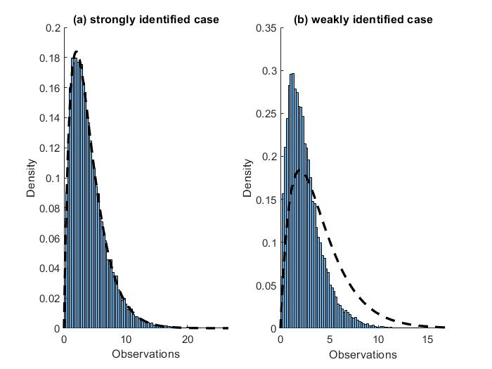
Figure 4: simulated density plots of the sFAR test statistic (shadowed bins) and the density function of the $\chi^{2}$-distribution (dashed black curve). The left panel (a) is the strong identified case, while the right panel (b) is the weak identified case.

Figure 4 illustrates the $\chi^{2}$ bound on the limiting distribution of the sFAR statistic stated in Proposition 5.2. The density of the limiting distribution of the sFAR statistic is simulated for a two-factor model, which uses the first two PCA factors to mimic the strongly identified case and the third and the fifth PCA factors to mimic weak identification. The limiting distribution of the sFAR statistic is $\chi^{2}$ when the model is strongly identified. In the weakly identified case, as shown in Figure 4, the limiting distribution is bounded by the $\chi^{2}$ distribution. Using $\chi^{2}$ critical values for the sFAR test thus controls the size of the test.

For projection-based tests on $\lambda_{1},$ the involved test has to be computed over a grid of points concerning the partialled out parameters. This becomes computationally burdensome when the number of partialled out parameters increases because of an increased dimension of $\Lambda_{1}$ resulting from more factors. It makes our proposed approach involving the sFAR test more empirically appealing because it does not involve an extensive grid search. In practice, Assumption 5.1 can be relaxed by using the KPST as a pre-test for conducting robust subset testing as described in Guggenberger et al. (2022).

The value of the sFAR statistic at parameter values distant from zero provide a diagnostic to indicate if the confidence sets of the hypothesized parameters are bounded. These tests are therefore indicative of weak identification.

Proposition 5.3.

For tests of $\text{H}_{0}:\lambda_{1}=c\lambda_{1}^{0}$ with $\lambda_{1}^{0}$ a fixed vector of length one and $c$ a scalar, $\lim_{c\rightarrow\infty}$ sFAR($c\lambda_{1}^{0}$), the realized value of the sFAR statistic at a distant value of $\lambda_{1}$ in the direction of $\lambda_{1}^{0}$, equals $T$ times the sum of the K smallest roots of

$$\begin{array}[]{rl}\left|\left(\begin{array}[]{cc}\bar{\lambda}_{1,\perp}^{0}&0\\ 0&I_{K}\end{array}\right)^{\prime}\left[\mu\hat{\Psi}-\hat{\Phi}^{\prime}\hat{\Sigma}^{-1}\hat{\Phi}\right]\left(\begin{array}[]{cc}\bar{\lambda}_{1,\perp}^{0}&0\\ 0&I_{K}\end{array}\right)\right|&=0,\end{array}$$

where $\bar{\lambda}_{1,\perp}^{0}$ is a $K\times(K-1)$ orthonormal matrix that is orthogonal to $\lambda_{1}^{0}$. The limit sFAR statistic is uniformly bounded from below by the minimum eigenvalue of $T\hat{\Psi}_{V}^{-1/2\prime}\hat{\beta}^{\prime}\hat{\Sigma}^{-1}\hat{\beta}\hat{\Psi}_{V}^{-1/2}$.

Proof.

See Appendix. ∎

Proposition 5.3 provides a way of verifying whether the confidence sets resulting from the sFAR statistic are bounded or unbounded in specific directions (Dufour (1997), Kleibergen and Zhan (2020), Kleibergen (2021), Khalaf and Schaller (2016), Kleibergen et al. (2022)). The minimum eigenvalue of $T\hat{\Psi}_{V}^{-1/2\prime}\hat{\beta}^{\prime}\hat{\Sigma}^{-1}\hat{\beta}\hat{\Psi}_{V}^{-1/2}$ is a rank test statistic concerning the rank of the factor loading matrix $\beta$ (see Kleibergen and Paap (2006)), so Proposition 5.3 shows that the sFAR test evaluated at distant values relates to the rank of $\beta.$ Proposition 5.3 also explains that when we encounter weak identification issues with $\beta$’s close to reduced rank, we have unbounded confidence sets. The lower bound is sharp when $K=1,$ as indicated in the proof of Proposition 5.3, for which case also Theorem 12 in Kleibergen (2021) applies. When $K=1$ and the Kleibergen-Paap rank test is significant at the 5% significance level, Proposition 5.3 implies that the sFAR test leads to bounded 95% confidence sets of $\lambda_{1}$.

Table 4 reports the Kleibergen-Paap rank test for different factor settings for the data from Adrian et al. (2013). It shows that, in line with Figure 3, all single-factor model have bounded 95% confidence sets for the time-varying risk premia, which are less likely to be bounded when we include more than three factors. The fifth factor, though identified in a single-factor setting, suffers from weak identification problems when we include other factors. Table 4 also shows that the rank test statistic is a good indicator of unboundedness as small values of the rank test statistics suggest unbounded confidence sets.

(1)	rank	(2)	rank	(3)	rank	(4)	rank	(5)	rank
	test		test		test		test		test
1*	30075	1,2	1290	1,2,3	711.1	1,2,3,	932.9	1,2,3,	9.105
	[0.000]		[0.000]		[0.000]	4	[0.000]	4,5$\dagger\dagger$	[0.003]
2*	4409	1,3	1487	1,2,4	1317	1,2,3,	5.103
	[0.000]		[0.000]		[0.000]	5$\dagger\dagger$	[0.078]
3*	973.0	1,4	1073	1,2,5	26.03	1,2,4,	76.53
	[0.000]		[0.000]		[0.002]	5	[0.000]
4*	703.2	1,5	39.82	1,3,4	603.8	1,3,4,	12.36
	[0.000]		[0.000]		[0.000]	5	[0.002]
5*	74.62	2,3	864.7	1,3,5	13.22	2,3,4,	16.23
	[0.000]		[0.000]		[0.004]	5	[0.000]
		2,4	990.9	1,4,5	110.3
			[0.000]		[0.000]
		2,5	63.17	2,3,4	765.8
			[0.000]		[0.000]
		3,4	825.2	2,3,5	16.96
			[0.000]		[0.001]
		3,5	11.14	2,4,5	549.0
			[0.025]		[0.000]
		4,5	445.2	3,4,5	18.05
			[0.000]		[0.000]

Table 4: Kleibergen-Paap rank statistic testing $H_{0}:\text{rank}(\beta)=K-1$ ($K$ denotes the number of factors) and its associated [$p$-value] in square brackets, for varying factor combinations. The colum headed by (i), for i=1,…,5, states which factor combinations are used when using i factors. All cases use excess returns on bonds with maturities of 2, 3, 12, 60, and 120 months and different combinations of the five PCA factors from Adrian et al. (2013). We mark with one star if the lower bound of the limit sFAR (see Proposition 5.3) indicates bounded 95% confidence sets in every direction, and mark with double daggers if the associated 95% confidence sets of the time-varying risk premia parameters of one or more factor are unbounded.

5.1 Power of the sFAR test

To illlustrate the power of the sFAR test, we compute power curves for two settings calibrated to the data discussed previously. Figure 6 therefore shows the two-dimensional power curves that result when jointly testing the two risk premia parameters associated with a single factor in a two factor model. The left hand side of Figure 6 shows the power curves for a strongly identified setting while the right hand side does so for a weakly identified setting. The power curves on the right hand side show that the sFAR test is not consistent for weakly identified settings since the rejection frequencies do not converge to one when we move away from the hypothesized value.

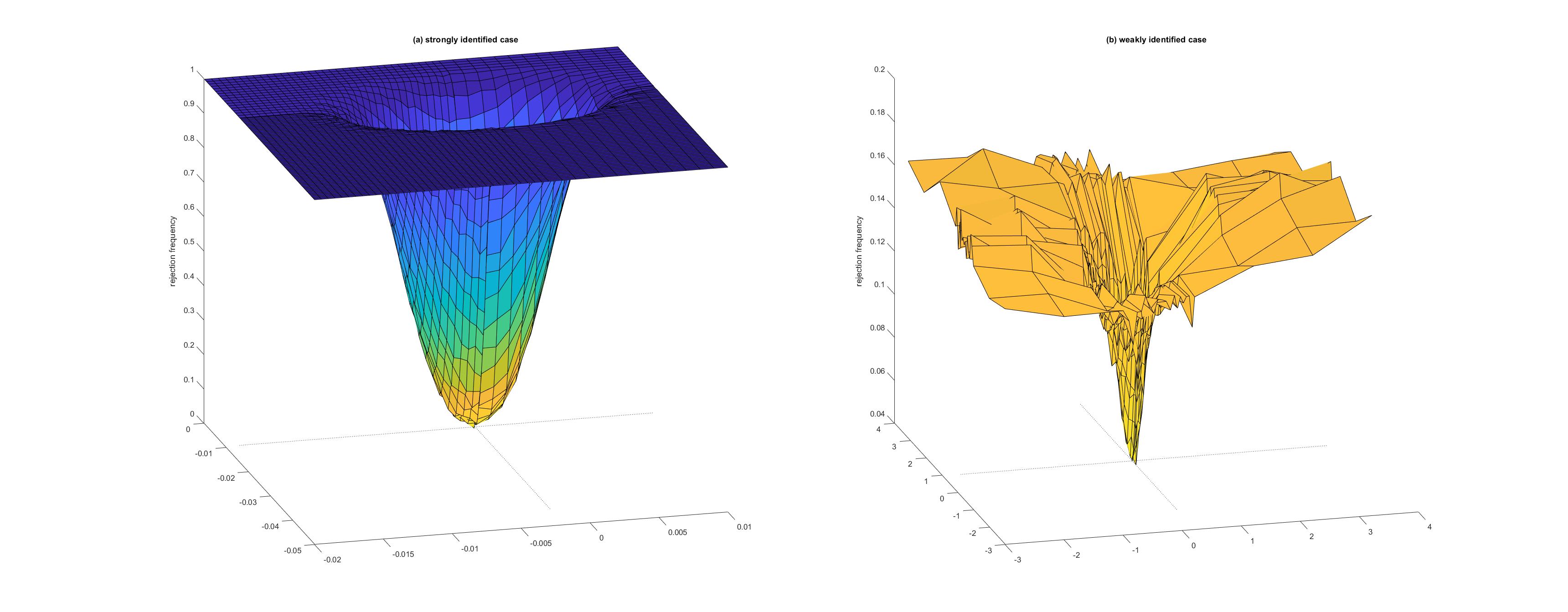
Figure 6: Simulated power surfaces (rejection frequencies) of sFAR tests on $\Lambda_{1}$’s w.r.t. the first factor of a two-factor model: the left panel (a) is a strong identified setting calibrated to the two-factor model with excess returns of bonds with maturities 3, 60, 120 months using the first and second PCA factors , while the right panel (b) is a weakly identified setting calibrated to the two-factor model with excess returns of bonds with maturities 3, 60, 120 months using the third and fifth PCA factors. Dotted lines $(\gamma_{i},y,0.05)$ are drawn to mark the positions of the calibrated risk premia values, $\gamma_{i}$’s, at 5% level.

5.2 Identification robust confidence sets for risk premia

We use the sFAR test to construct confidence sets on the risk premia resulting from two and three factor models. Figure 7 shows the 90, 95 and 99% joint confidence sets that result for the two risk premia resulting for one specific factor in a two factor model using the data from Adrian et al. (2013) while Figure 8 does so for the three risk premia resulting for one specific factor in a three factor model. Size correct confidence sets for the individual risk premia result by projecting the joint confidence sets on the axes. When using four or more factors, the number of risk premia concerning one factor is at least four so we have to use projection-based tests based on the sFAR statistic to be able to visualize these confidence sets. For expository purposes and since Table 4 shows that some of these confidence sets are unbounded, for example, the one that results when using all five factors, we therefore refrain from using more than three factors.

Figure 7 shows all two dimensional confidence sets for the two risk premia resulting for one factor for all different specifications using the five PCA factors discussed previously in a two factor model. The two dimensional confidence sets in Figure 2 vary a lot. Quite a few are empty so all values of the parameters are rejected at significance levels which exceed 99%. This occurs, for example, when using the first and either the second, third and fourth PCA factor so the model is misspecified. There are also settings where the confidence set is bounded and well behaved which occurs, for example, when using the third and fourth PCA factor. Other confidence sets are unbounded and/or cover the whole two-dimensional space, which occurs, for instance, when using the third and fifth PCA. For this combination the 90% confidence set for the two risk premia on the third factor is unbounded but excludes an area in the parameter space while the 90% confidence set of the two risk premia on the fifth factor covers the whole two-dimensional space. Table 4 also shows that the combination of the third and fifth PCA factors leads to a smaller rank test statistic than other factor combinations when using two-factor models which is in line with the unbounded confidence set in Figure 7 which relates to the third and fifth PCA factors. This is all indicative of weak identification when using both the third and fifth factors.

Figure 8 shows the joint confidence sets for the three risk premia associated with a single factor in a three factor model. The first column of Figure 8 does for a factor model containing the first three PCAs as factors while the second column does so using the first, third and fifth PCAs as factors. Unlike when using two factors, the first column shows that the confidence sets are no longer empty but bounded which shows that the risk premia for the first three PCA factors are well identified and that the model is no longer misspecified. This is confirmed by the p-value of the rank test on the $\beta$’s. This is in contrast when using the first, third and fifth PCAs as factors. The confidence sets in the second column of Figure 8 are namely all unbounded indicating weak identification of the risk premia which is further reflected by the $p$-value of the rank test on the $\beta$’s. Table 4 also shows that the model including the first, third, and fifth PCA factors has a much smaller rank test statistic than one of the first three PCA factors within the three-factor model. 

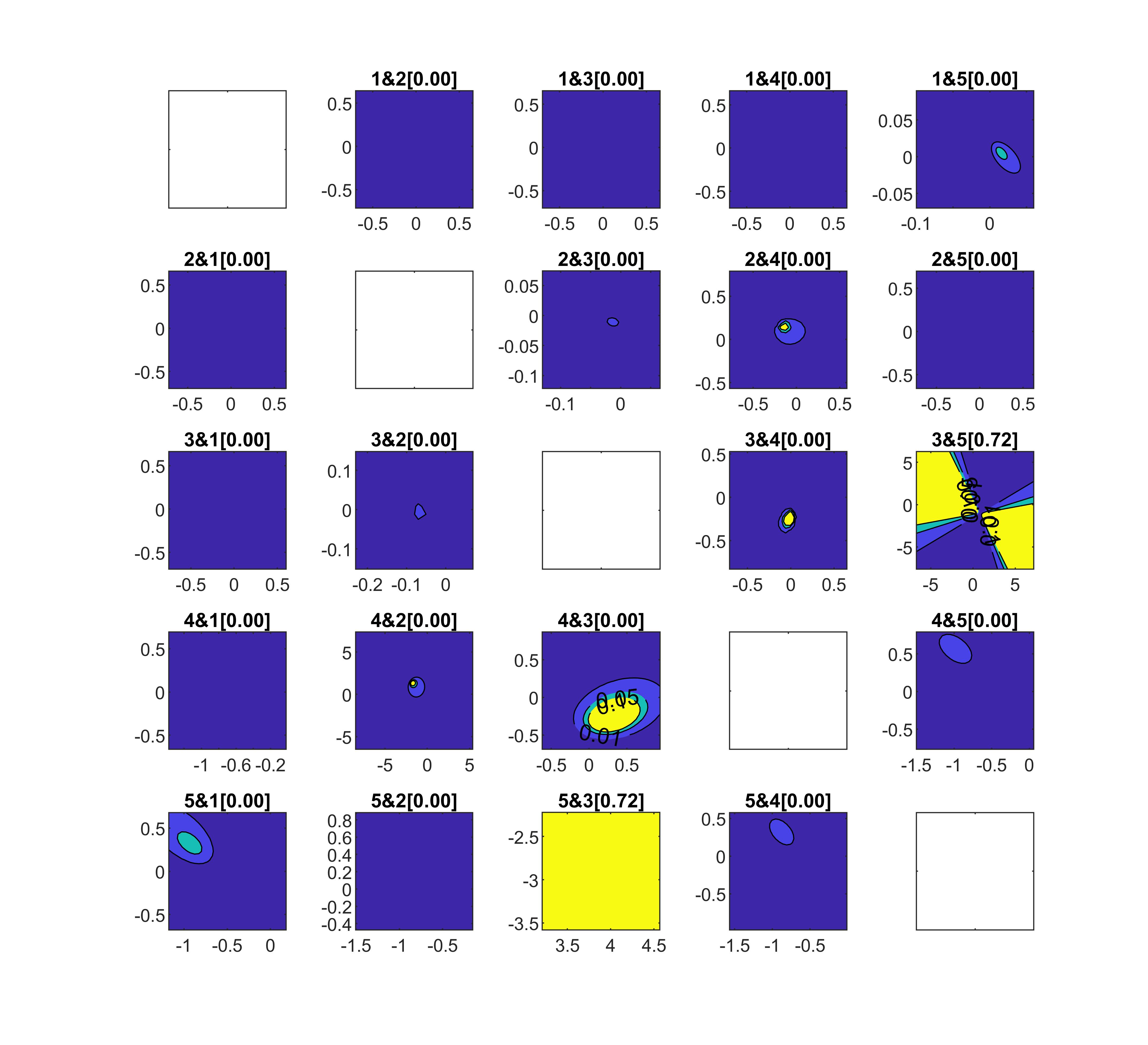
Figure 7: Joint confidence sets from the sFAR test for the two risk premia of the first of the two listed factors in a two factor model. (yellow 90%, light green 95%, light blue 99%, dark blue area contains the remaining values). Excess returns on bonds with maturities 3, 60, 120 months are used. [$p$-value] of Kleibergen-Paap rank statistic testing $H_{0}:\text{rank}(\beta)=1$ in square brackets.

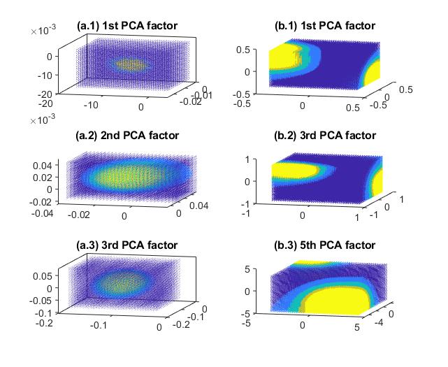
Figure 8: Joint confidence sets from the sFAR test for three-factor models (yellow 90%, light green 95%, light blue 99%, dark blue area contains the remaining values) with excess returns on bonds with maturities 3, 60, 120 months, (a.i) testing on $\Lambda_{1}$’s w.r.t. the $i$-th factor when using first, second and third PCA factors factors Kleibergen-Paap rank statistic testing $H_{0}$ :rank($\beta$)=2 equals 310.9294 [p-value: 0.0000]); (b.i) testing on $\Lambda_{1}$’s w.r.t. the $($$i+2)$-th factor when using first, third and fifth PCA factors factors. Kleibergen-Paap rank statistic testing $H_{0}$ :rank($\beta$)=2 equals 0.0654 [p-value 0.7981]).

Figure 8 shows the three dimensional confidence sets that result from the sFAR test. It results from partialling out the six risk premia associated with the other factors. Hence, when we compute these confidence sets using projection with the identification robust tests, we have to specify a nine-dimensional grid for the risk premia and compute the identification robust tests for all values on this nine-dimensional grid. This is, or is close to be, computationally infeasible. Hence, the sFAR test provides a computationally tractable manner to conduct identification robust tests on larger number of parameters.

6 Conclusion

We propose identification robust test procedures for testing hypotheses on risk premia in dynamic affine term structure models. The robust subset factor Anderson-Rubin test extends the sFAR test from the linear asset pricing model to allow for tests on multiple risk premia and, unlike projection based testing, provides a computationally tractable manner to conduct identification robust tests on larger number of parameters. Our empirical results show that especially in case of multiple factors, weak identification is pervasive and traditional tests are likely misleading. We use the empirical settings from the literature on affine term structure models, see e.g. Adrian et al. (2013) and Ang and Piazzesi (2003)), to illustrate our results and the importance of using weak identification robust test procedures.

Appendix A Appendix: Proofs.

A.1 Proof of Proposition 5.1.

Suppose that there exists a consistent estimator for $S$, $\hat{S}$, a by-product of the KPS test is the KPS factorization for $\hat{S}$ (Guggenberger et al.(2022)). We briefly discuss how it operates. For a matrix $A\in\mathbb{R}^{kp\times kp}$ with a block structure

$$R:=\left(\begin{array}[]{ccc}R_{11}&\cdots&R_{1p}\\ \vdots&\ddots&\vdots\\ R_{p1}&\cdots&R_{pp}\end{array}\right)$$

where $R_{jl}\in\mathbb{R}^{k\times k},j,l=1,\ldots,p$, define

$$\mathcal{R}(A):=\left(\begin{array}[]{c}\displaystyle A_{1}\\ \vdots\\ A_{p}\end{array}\right)\in\mathbb{R}^{p^{2}\times k^{2}},$$

with

$$A_{j}:=\left(\begin{array}[]{c}\displaystyle\text{vec}\left(A_{1j}\right)^{\prime}\\ \vdots\\ \text{vec}\left(A_{pj}\right)^{\prime}\end{array}\right)\in\mathbb{R}^{p\times k^{2}}$$

for $j=1,\ldots,p$. Consider a singular value decomposition (SVD) of $\mathcal{R}(\hat{S})$:

$$\mathcal{R}(\hat{S})=\hat{L}\hat{\Sigma}\hat{N}^{\prime}$$

where $p=2K,$ $k=N$, $\hat{\Sigma}:=\text{diag}\left(\hat{\sigma}_{1}\ldots\hat{\sigma}_{\min\left(p^{2},k^{2}\right)}\right)$ denotes a $p^{2}\times k^{2}$ dimensional diagonal matrix with the singular values $\hat{\sigma}_{j}$ $\left(j=1,\ldots,\min\left(p^{2},k^{2}\right)\right)$ non-increasingly ordered on the main diagonal, and $\hat{L}\in$ $\mathbb{R}^{p^{2}\times p^{2}},$ $\hat{N}\in\mathbb{R}^{k^{2}\times k^{2}}$ orthonormal matrices. Decompose

$$\begin{array}[]{c}\hat{L}:=\left(\begin{array}[]{ll}\displaystyle\hat{L}_{11}&\hat{L}_{12}\\ \hat{L}_{21}&\hat{L}_{22}\end{array}\right)=\left(\hat{L}_{1}\text{ }\vdots\text{ }\hat{L}_{2}\right),\hat{\Sigma}:=\left(\begin{array}[]{cc}\hat{\sigma}_{1}&0\\ 0&\hat{\Sigma}_{2}\end{array}\right),\\ \hat{N}:=\left(\begin{array}[]{ll}\displaystyle\hat{N}_{11}&\hat{N}_{12}\\ \hat{N}_{21}&\hat{N}_{22}\end{array}\right)=\left(\hat{N}_{1}\text{ }\vdots\text{ }\hat{N}_{2}\right)\end{array}$$

with $\hat{L}_{11}:1\times 1,$ $\hat{L}_{12}:1\times\left(p^{2}-1\right),$ $\hat{L}_{21}:\left(p^{2}-1\right)\times 1,$ $\hat{L}_{22}:\left(p^{2}-1\right)\times\left(p^{2}-1\right),$ $\hat{\sigma}_{1}:1\times 1$, $\hat{\Sigma}_{2}:\left(p^{2}-1\right)\times\left(k^{2}-1\right),$ $\hat{N}_{11}:1\times 1,$ $\hat{N}_{12}:1\times\left(k^{2}-1\right),$ $\hat{N}_{21}:\left(k^{2}-1\right)\times 1,$ $\hat{N}_{22}:\left(k^{2}-1\right)\times\left(k^{2}-1\right)$ dimensional matrices. The consistency follows from the consistency of $\hat{S}$ and Theorem 1 from Guggenberger et al. (2022).
$\square$

A.2 Intermediate results for the Proof of Proposition 5.2 .

We show some intermediate results needed for the proof of Proposition 5.2. To prove that critical values from a $\chi^{2}$-distribution serve as a proper upper bound, we extend the methodology employed in Guggenberger et al. (2019) by linking the test statistic to the smaller roots of an eigenvalue problem and thereafter analyzing the distributions of the eigenvalues.

We first provide Proposition A.1 below which shows that for the upper bound, we only need to consider the distribution of the $K$ smallest roots of $\left|\mu I_{2K-1}-\Xi^{\prime}\Xi\right|=0$ , where $\Xi^{\prime}\Xi\sim_{a}\mathcal{W}_{2K-1}\left(N,I_{2K-1},\mathcal{M}^{\prime}\mathcal{M}\right)$, for the “strongly identified” setting and $\mathcal{W}_{2K-1}\left(N,I_{2K-1},\mathcal{M}^{\prime}\mathcal{M}\right)$ indicates a non-central Wishart distribution of a $(2K-1)\times(2K-1)$ dimensional matrix with $N$ degrees of freedom, scaling matrix $I_{2K-1}$ and non-centrality $\mathcal{M}^{\prime}\mathcal{M}$. Proposition A.1.1 together with its proof show that the sFAR statistic results from an eigenvalue problem as the summation of its $K$ smallest eigenvalues. We can thus focus on the joint distribution of these smallest eigenvalues to obtain the distributional behavior of the sFAR statistic.

Proposition A.1.1 shows that the distribution of the eigenvalues under the null hypothesis depends only on the nuisance parameters $\mathcal{M}$. Proposition A.1.3 argues that to derive the upper bound, we need only focus on the nuisance parameters $\mathcal{M}$ under the “strongly identified” setting, where the eigenvalues of $\mathcal{M}^{\prime}\mathcal{M}$ satisfy the condition that $\kappa_{1}>\kappa_{2}>\cdots>\kappa_{K-1}>\kappa_{K}=\kappa_{K+1}=\cdots=0$ and the $(K-1)$-th largest eigenvalue, $\kappa_{K-1}$, goes to infinity. Because the “strongly identified” is shown to lead to the “largest probability” of having larger values of the $K$ smallest eigenvalues.

In the following, we first provide Proposition A.1 and then continue to discuss the joint distribution of the eigenvalues of the eigenvalue problem from Proposition A.1.1 and the associated approximate conditional distribution of the smallest eigenvalues in Section A.2.1.

Proposition A.1.

Under Assumptions of Proposition 5.2,

1. The sFAR$(\lambda_{1}^{0})$ statistic equals the sum of the K smallest roots of the following polynomial: $\left|\mu I_{2K-1}-\Xi^{\prime}\Xi\right|=0$, where

   $$\begin{array}[]{rl}\displaystyle\Xi=&\left[\xi_{u}\text{ }\vdots\text{ }\xi_{\beta_{2}}\right]\sim_{a}N\left(\mathcal{M},I_{N(2K-1)}\right),\\ \displaystyle\sqrt{T}\hat{\Sigma}^{-\frac{1}{2}}\hat{u}\hat{\Psi}_{uu}^{-\frac{1}{2}}\underset{d}{\rightarrow}&\xi_{u}\\ \displaystyle\sqrt{T}\hat{\Sigma}^{-\frac{1}{2}}\left(\hat{\beta}_{2}-\hat{u}\hat{\Psi}_{uu}^{-1}\hat{\Psi}_{u\beta_{2}}^{\prime}\right)\hat{\Psi}_{\beta_{2}\beta_{2}\cdot u}^{-\frac{1}{2}}\underset{d}{\rightarrow}&\xi_{\beta_{2}}\\ \displaystyle\mathcal{M}=&\left(\sqrt{T}{\Sigma}^{-\frac{1}{2}}\beta_{1}(\lambda_{1}-\lambda_{1}^{0})^{\prime}{\Psi}_{uu}^{-\frac{1}{2}}\text{ }\vdots\right.\\ \displaystyle\hfil&\left.\sqrt{T}{\Sigma}^{-\frac{1}{2}}\left({\beta}_{2}-\beta_{1}(\lambda_{1}-\lambda_{1}^{0})^{\prime}{\Psi}_{uu}^{-1}{\Psi}_{u\beta_{2}}^{\prime}\right){\Psi}_{\beta_{2}\beta_{2}\cdot u}^{-\frac{1}{2}}\right),\end{array}$$

   and “$\sim_{a}$” denotes an approximate distribution in large samples, and ${\Psi}_{uu}$, ${\Psi}_{u\beta_{2}}$, ${\Psi}_{\beta_{2}\beta_{2}\cdot u},$ $\hat{\Psi}_{uu}$, $\hat{\Psi}_{u\beta_{2}}$, $\hat{\Psi}_{\beta_{2}\beta_{2}\cdot u}$ are specified in the proof.

2. Let $\hat{\kappa}_{1}\geq\hat{\kappa}_{2}\geq\cdots\geq\hat{\kappa}_{2K-1}$ be the eigenvalues of $\Xi^{\prime}\Xi$, and ${\kappa}_{1}\geq{\ \ \kappa}_{2}\geq\cdots\geq{\kappa}_{2K-1}$ be the eigenvalues of $\mathcal{M}^{\prime}\mathcal{M}$. Under the hypothesis $H_{0}:\lambda_{1}=\lambda_{1}^{0}$, $\hat{\kappa}_{j}=O_{p}(1),$ $j=K,\cdots,2K-1$; and when $\kappa_{K-1}\rightarrow\infty$, we have $\hat{\kappa}_{i}\rightarrow_{p}\infty,i=1,\cdots,K-1.$

3. $\{\mathcal{M}_{n},n\geq 1\}$ is a sequence of the parameter matrix $\mathcal{M}$, and let $\mathbb{M}$ denote the collection of all such sequences. $\mathbb{M}_{\infty}$ is a subset of $\mathbb{M}$ that is a collection of $\{\mathcal{M}_{n},n\geq 1:\kappa_{1}(\mathcal{M}_{n}^{\prime}\mathcal{M}_{n})>\cdots>\kappa_{K-1}(\mathcal{M}_{n}^{\prime}\mathcal{M}_{n})>\kappa_{K}(\mathcal{M}_{n}^{\prime}\mathcal{M}_{n})=\kappa_{K+1}(\mathcal{M}_{n}^{\prime}\mathcal{M}_{n})=\cdots=0,\kappa_{K-1}(\mathcal{M}_{n}^{\prime}\mathcal{M}_{n})\rightarrow\infty\}$. Let $\tilde{\Xi}_{\mathcal{M}}=Z+\mathcal{M}$ with $Z\sim N(0,I)$ ,then under the hypothesis $H_{0}:\lambda_{1}=\lambda_{1}^{0}$, for any $\{\mathcal{M}_{n},n\geq 1\}\in\mathbb{M}$, we can find a parameter sequence $\{\tilde{\mathcal{M}}_{h},h\geq 1\}\in\mathbb{M}_{\infty}$ such that

   $$\begin{array}[]{cl}\displaystyle\limsup\limits_{n\rightarrow\infty}\hat{\kappa}_{j}(\tilde{\Xi}_{\mathcal{M}_{n}}^{\prime}\tilde{\Xi}_{\mathcal{M}_{n}})\leq\liminf\limits_{h\rightarrow\infty}\hat{\kappa}_{j}(\tilde{\Xi}_{\tilde{\mathcal{M}}_{h}}^{\prime}\tilde{\Xi}_{\tilde{\mathcal{M}}_{h}}),j\geq K.&\end{array}$$

Proof of Proposition A.1.

Proof of A.1.1.

The FAR statistic reads as follows

$$\begin{array}[]{cl}\displaystyle\text{FAR(}{\Lambda}_{1}^{0}\mathbf{)=}&{T\times f}_{T}{(\Lambda}_{1}^{0}{,X)}^{\prime}{\hat{V}}_{ff}{(\Lambda}_{1}^{0}{)}^{-1}{f}_{T}{(\Lambda}_{1}^{0}{,X)},\end{array}$$ (A.1)

and the sample moments $f_{T}(\Lambda_{1},X)$ of the model under consideration for given $\Lambda_{1}$ are

$$\begin{array}[]{c}\displaystyle f_{T}(\Lambda_{1},X)=\frac{1}{T}\sum_{t=1}^{T}(\bar{X}_{t-1}\otimes(\bar{R}_{t}-\hat{\beta}\hat{V}_{t}))-\left(\hat{Q}_{XX}\otimes\hat{\beta}\right)\text{vec(}\Lambda_{1}).\end{array}$$

Note that for $\hat{d}$ the least squares estimator resulting from the 2-nd step of the three step procedure,

$$\begin{array}[]{c}\displaystyle\left(\hat{Q}_{XX}\otimes I_{N}\right)^{-1}\frac{1}{T}\sum_{t=1}^{T}(\bar{X}_{t-1}\otimes(\bar{R}_{t}-\hat{\beta}\hat{V}_{t}))=\text{vec}(\hat{d}),\end{array}$$

which implies that

$$\begin{array}[]{c}\displaystyle f_{T}(\Lambda_{1},X)=\left(\hat{Q}_{XX}\otimes I_{N}\right)\text{vec}\left(\hat{\Phi}A(\lambda_{1})\pi_{\Lambda_{2}}\right),\end{array}$$ (A.2)

with

$$\begin{array}[]{c}\hat{\Phi}=\frac{1}{T}\sum_{t=1}^{T}R_{t}\left(\begin{array}[]{c}\bar{X}_{t}\\ \hat{v}_{t+1}\end{array}\right)^{\prime}\left[\frac{1}{T}\sum_{t=1}^{T}\left(\begin{array}[]{c}\bar{X}_{t}\\ \hat{v}_{t+1}\end{array}\right)\left(\begin{array}[]{c}\bar{X}_{t}\\ \hat{v}_{t+1}\end{array}\right)^{\prime}\right]^{-1}=\left(\hat{d}\ \text{{}}\vdots\ \text{{}}\hat{\beta}\right)\\ \displaystyle A(\lambda_{1})=\left(\begin{array}[]{ccc}I_{K}&-\lambda_{1}&0\\ 0&0&I_{K-1}\end{array}\right)^{\prime},\text{ }\pi_{\Lambda_{2}}=\left(\begin{array}[]{c}I_{K}\\ -\Lambda_{2}\end{array}\right).\end{array}$$

Provided that Assumption 5.1 holds, the above result implies that we can choose

$$\begin{array}[]{c}\hat{V}_{ff}{(\Lambda}_{1}^{0})=\left(\hat{Q}_{XX}\pi_{\Lambda_{2}^{0}}^{\prime}A(\lambda_{1}^{0})^{\prime}\otimes I_{N}\right)\hat{V}_{\hat{\Phi}}\left(A(\lambda_{1}^{0})\pi_{\Lambda_{2}^{0}}\hat{Q}_{XX}\otimes I_{N}\right)\\ =\left(\hat{Q}_{XX}\otimes I_{N}\right)\left(\pi_{\Lambda_{2}^{0}}^{\prime}A(\lambda_{1}^{0})^{\prime}\hat{\Psi}A(\lambda_{1}^{0})\pi_{\Lambda_{2}^{0}}\otimes\hat{\Sigma}\right)\left(\hat{Q}_{XX}\otimes I_{N}\right).\end{array}$$ (A.3)

Substituting (A.2) and (A.3) into (A.1) gives

$$\begin{array}[]{c}\displaystyle\text{FAR(}\lambda_{1}^{0},\Lambda_{2}^{0})\\ =T\text{vec}\left(\hat{\Phi}A(\lambda_{1})\pi_{\Lambda_{2}}\right)^{\prime}\left(\pi_{\Lambda_{2}^{0}}^{\prime}A(\lambda_{1}^{0})^{\prime}\hat{\Psi}A(\lambda_{1}^{0})\pi_{\Lambda_{2}^{0}}\otimes\hat{\Sigma}\right)^{-1}\text{vec}\left(\hat{\Phi}A(\lambda_{1})\pi_{\Lambda_{2}}\right)\\ =T\text{vec}\left(\hat{\Phi}A(\lambda_{1})\pi_{\Lambda_{2}}\right)^{\prime}\text{vec}\left(\hat{\Sigma}^{-1}\hat{\Phi}A(\lambda_{1})\pi_{\Lambda_{2}}\left(\pi_{\Lambda_{2}^{0}}^{\prime}A(\lambda_{1}^{0})^{\prime}\hat{\Psi}A(\lambda_{1}^{0})\pi_{\Lambda_{2}^{0}}\right)^{-1}\right),\end{array}$$

which via the trace operator can be rewritten as

$$\begin{array}[]{l}\displaystyle\text{FAR(}\lambda_{1}^{0},\Lambda_{2}^{0})=T\text{tr}\left(\pi_{\Lambda_{2}^{0}}^{\prime}A(\lambda_{1}^{0})^{\prime}\hat{\Phi}^{\prime}\hat{\Sigma}^{-1}\hat{\Phi}A(\lambda_{1}^{0})\pi_{\Lambda_{2}^{0}}\left[\pi_{\Lambda_{2}^{0}}^{\prime}A(\lambda_{1}^{0})^{\prime}\hat{\Psi}A(\lambda_{1}^{0})\pi_{\Lambda_{2}^{0}}\right]^{-1}\right).\end{array}$$

Denote

$$\begin{array}[]{l}\displaystyle\widetilde{\text{FAR}}(\lambda_{1}^{0},q)=T\text{tr}\left(q^{\prime}A(\lambda_{1}^{0})^{\prime}\hat{\Phi}^{\prime}\hat{\Sigma}^{-1}\hat{\Phi}A(\lambda_{1}^{0})q\left[q^{\prime}A(\lambda_{1}^{0})^{\prime}\hat{\Psi}A(\lambda_{1}^{0})q\right]^{-1}\right),\end{array}$$

where $q$ is a $(2K-1)\times K$ matrix of full column rank $K$. Let $q^{\ast}$ denote the set of $(2K-1)\times K$ matrices of full column rank $K$, and $q^{\ast\ast}$ denote the set of all matrices $q$ for which $q^{\prime}A(\Lambda_{0})^{\prime}\hat{\Psi}A(\Lambda_{0})q=I_{K}$, then it is a straightforward result such that

$$\begin{array}[]{c}\displaystyle\min_{q\in q^{\ast}}\widetilde{\text{FAR}}(\lambda_{1}^{0},q)=\min_{q\in q^{\ast\ast}}\displaystyle\widetilde{\text{FAR}}(\lambda_{1}^{0},q)\leq\inf_{\Lambda_{2}^{0}}\text{FAR(}\lambda_{1}^{0},\Lambda_{2}^{0}).\end{array}$$

Denote $\hat{q}=\arg\min_{q\in q^{\ast\ast}}\displaystyle\widetilde{\text{FAR}}(\lambda_{1}^{0},q)$, and we prove A.1.1 by linking $\widetilde{\text{FAR}}(\lambda_{1}^{0},\hat{q})$ with an eigenvalue problem and showing that under the null hypothesis $\lambda_{1}=\lambda_{1}^{0}$, with probability approaching one we have

$$\begin{array}[]{c}\inf_{\Lambda_{2}^{0}}\text{FAR(}\lambda_{1}^{0},\Lambda_{2}^{0})=\widetilde{\text{FAR}}(\lambda_{1}^{0},\hat{q}).\end{array}$$ (A.4)

Theorem 1.2 from Sameh and Wisniewski (1982) implies that $\widetilde{\text{FAR}}(\lambda_{1}^{0},\hat{q})$ equals $T$ times the sum of the $K$ smallest eigenvalues of the eigenvalue problem:

$$\begin{array}[]{c}A(\Lambda_{0})^{\prime}\hat{\Phi}^{\prime}\hat{\Sigma}^{-1}\hat{\Phi}A(\Lambda_{0})x=\kappa\hat{\Psi}(\lambda_{1}^{0})x,\end{array}$$

where $\hat{\Psi}(\lambda_{1}^{0})=A(\Lambda_{0})^{\prime}\hat{\Psi}A(\Lambda_{0})$, $x$ is a $(2K-1)$-eigenvector, $\kappa$ is a scalar eigenvalue. $T$ times the sum of the $K$ smallest eigenvalues, $\kappa$’s, of the above eigenvalue problem equals $T$ times the sum of the $K$ smallest roots of the characteristic polynomial:

$$\begin{array}[]{lc}\displaystyle\left|\mu\hat{\Psi}(\lambda_{1}^{0})-A(\Lambda_{0})^{\prime}\hat{\Phi}^{\prime}\hat{\Sigma}^{-1}\hat{\Phi}A(\Lambda_{0})\right|=0.&\end{array}$$ (A.5)

Pre/post-multiplying $\displaystyle\left|\mu\hat{\Psi}(\lambda_{1}^{0})-TA(\Lambda_{0})^{\prime}\hat{\Phi}^{\prime}\hat{\Sigma}^{-1}\hat{\Phi}A(\Lambda_{0})\right|=0$ by $\displaystyle\left(\begin{array}[]{cc}I_{K}&-\Lambda_{2}^{\prime}\\ 0&I_{K-1}\end{array}\right)$ gives

$$\begin{array}[]{lc}\displaystyle\left|\mu\hat{\Psi}(\lambda_{1}^{0},\Lambda_{2})-T\left(\hat{u},\hat{\beta}_{2}\right)^{\prime}\hat{\Sigma}^{-1}\left(\hat{u},\hat{\beta}_{2}\right)\right|&=0\end{array},$$ (A.6)

where

$$\begin{array}[]{cc}\displaystyle\hat{\Psi}(\lambda_{1}^{0},\Lambda_{2})=\left(\begin{array}[]{cc}I_{K}&-\Lambda_{2}^{\prime}\\ 0&I_{K-1}\end{array}\right)^{\prime}\hat{\Psi}(\lambda_{1}^{0})\left(\begin{array}[]{cc}I_{K}&-\Lambda_{2}^{\prime}\\ 0&I_{K-1}\end{array}\right)=\left(\begin{array}[]{cc}\hat{\Psi}_{u}&\hat{\Psi}_{u\beta_{2}}\\ \hat{\Psi}_{u\beta_{2}}^{\prime}&\hat{\Psi}_{\beta_{2}}\end{array}\right),&\end{array}$$

and $\hat{u}=\hat{d}-\hat{\beta}_{1}\lambda_{1}^{0\prime}-\hat{\beta}_{2}\Lambda_{2}=\epsilon+\hat{\beta}_{1}\left(\lambda_{1}-\lambda_{1}^{0}\right)^{\prime}.$ Note that $C\hat{\Psi}(\lambda_{1}^{0},\Lambda_{2})C^{\prime}=I_{2K-1}$ holds with

$$\begin{array}[]{lc}\displaystyle C=\left(\begin{array}[]{cc}\hat{\Psi}_{uu}^{-\frac{1}{2}}&0\\ -\hat{\Psi}_{\beta_{2}\beta_{2}\cdot u}^{-\frac{1}{2}}\hat{\Psi}_{u\beta_{2}}^{\prime}\hat{\Psi}_{uu}^{-1}&\hat{\Psi}_{\beta_{2}\beta_{2}\cdot u}^{-\frac{1}{2}}\end{array}\right),\displaystyle\hat{\Psi}_{\beta_{2}\beta_{2}\cdot u}=\hat{\Psi}_{\beta_{2}\beta_{2}}-\hat{\Psi}_{u\beta_{2}}^{\prime}\hat{\Psi}_{uu}^{-1}\hat{\Psi}_{u\beta_{2}}.&\end{array}$$

Pre/post-multiplying equation (A.6) by $|C|$ yields $\left|\mu I_{2K-1}-\Xi^{\prime}\Xi\right|=0$. Therefore, the eigenvalue problem (A.5) is equivalent to the eigenvalue problem $\left|\mu I_{2K-1}-\Xi^{\prime}\Xi\right|=0$, and $\widetilde{\text{FAR}}(\lambda_{1}^{0},\hat{q})$ equals the sum of the K smallest eigenvalues of $\Xi^{\prime}\Xi$.

Next, we complete the proof by showing that (A.4) holds. Denote $\hat{q}=\left(\hat{q}_{1}^{\prime},\hat{q}_{2}^{\prime}\right)^{\prime}$ with $\hat{q}_{1}$ a $K\times K$ submatrix of $\hat{q}$, and denote $\sigma_{i}(\hat{q}_{1}),i=1,\cdots K$ the singular values of $\hat{q}_{1}$ in descending order.

If $\hat{q}_{1}$ is of full rank, then by construction

$$\begin{array}[]{c}\text{FAR(}\lambda_{1}^{0},-\hat{q}_{2})\\ =T\text{tr}\left(\pi_{-\hat{q}_{2}}^{\prime}A(\Lambda_{0})^{\prime}\hat{\Phi}^{\prime}\hat{\Sigma}^{-1}\hat{\Phi}A(\Lambda_{0})\pi_{-\hat{q}_{2}}\left[\pi_{-\hat{q}_{2}}^{\prime}A(\Lambda_{0})^{\prime}\hat{\Psi}A(\Lambda_{0})\pi_{-\hat{q}_{2}}\right]^{-1}\right)\\ =T\text{tr}\left(A_{\hat{q}_{1}}^{\prime}\pi_{-\hat{q}_{2}}^{\prime}A(\Lambda_{0})^{\prime}\hat{\Phi}^{\prime}\hat{\Sigma}^{-1}\hat{\Phi}A(\Lambda_{0})A_{\hat{q}_{1}}\pi_{-\hat{q}_{2}}\left[A_{\hat{q}_{1}}^{\prime}\pi_{-\hat{q}_{2}}^{\prime}A(\Lambda_{0})^{\prime}\hat{\Psi}A(\Lambda_{0})\pi_{-\hat{q}_{2}}A_{\hat{q}_{1}}\right]^{-1}\right)\\ =\widetilde{\text{FAR}}(\lambda_{1}^{0},\hat{q}),\end{array}$$

where $A_{\hat{q}_{1}}=\left(\begin{matrix}\hat{q}_{1}&0\\ 0&I_{K-1}\end{matrix}\right)$. Hence, $\inf_{\Lambda_{2}^{0}}\text{FAR(}\lambda_{1}^{0},\Lambda_{2}^{0})=\widetilde{\text{FAR}}(\lambda_{1}^{0},\hat{q})$ when $\hat{q}_{1}$ is of full rank.

If $\hat{q}_{1}$ is not of full rank, consider a small-$\tilde{\epsilon}$ perturbation of $\hat{q}$, $\hat{q}_{\tilde{\epsilon}}=\hat{q}+\tilde{\epsilon}\pi_{\Lambda_{2}^{0}}=\left(\hat{q}_{\tilde{\epsilon},1}^{\prime},\hat{q}_{\tilde{\epsilon},2}^{\prime}\right)^{\prime}$, where $\hat{q}_{\tilde{\epsilon},1}$ is of full rank. We show that $\tilde{\epsilon}$ can be chosen in a way such that $\widetilde{\text{FAR}}(\lambda_{1}^{0},\hat{q})$ can be arbitrarily close to $\widetilde{\text{FAR}}(\lambda_{1}^{0},\hat{q}_{\tilde{\epsilon}})$, then from $\inf_{\Lambda_{2}^{0}}\text{FAR(}\lambda_{1}^{0},\Lambda_{2}^{0})\leq\widetilde{\text{FAR}}(\lambda_{1}^{0},\hat{q}_{\tilde{\epsilon}})$ we know $\inf_{\Lambda_{2}^{0}}\text{FAR(}\lambda_{1}^{0},\Lambda_{2}^{0})=\widetilde{\text{FAR}}(\lambda_{1}^{0},\hat{q})$. For example, let $\tilde{\epsilon}_{\delta}=-\min\left\{\delta,\frac{1}{2}|\sigma_{i}(\hat{q}_{1})|,i=1,\cdots,K\right\}$ with $\delta$ an arbitrary positive number. Then $\sigma_{i}(\hat{q}_{\tilde{\epsilon}_{\delta},1})\neq 0$ due to the extension of Weyl’s eigenvalue perturbation inequality to perturbation of singular values, and thus $\hat{q}_{\tilde{\epsilon}_{\delta},1}$ is of full rank, which leads to

$$\inf_{\Lambda_{2}^{0}}\text{FAR(}\lambda_{1}^{0},\Lambda_{2}^{0})\leq\text{FAR(}\lambda_{1}^{0},-\hat{q}_{\tilde{\epsilon}_{\delta},2})=\widetilde{\text{FAR}}(\lambda_{1}^{0},\hat{q}_{\tilde{\epsilon}_{\delta}}).$$

By construction, $\widetilde{\text{FAR}}(\lambda_{1}^{0},\hat{q}_{\tilde{\epsilon}_{\delta}})=\widetilde{\text{FAR}}(\lambda_{1}^{0},\hat{q})+O_{p}(\delta^{2})$ and since $\delta$ can be chosen arbitrarily small (e.g., $\delta=1/\sqrt{T}$), we know with probability approaching to one, $\inf_{\Lambda_{2}^{0}}\text{FAR(}\lambda_{1}^{0},\Lambda_{2}^{0})=\widetilde{\text{FAR}}(\lambda_{1}^{0},\hat{q})$ holds.

Proof of A.1.2.

Under the hypothesis $H_{0}:\lambda_{1}=\lambda_{1}^{0}$, we have $\mathcal{M}=\left(0_{N\times K},\sqrt{T}{\Sigma}^{-\frac{1}{2}}{\beta}_{2}{\Psi}_{\beta_{2}\beta_{2}\cdot u}^{-\frac{1}{2}}\right)$, and thus the rank of $\mathcal{M}$, denoted as $\rho(\mathcal{M})$, is smaller than or equal to $K-1$. Therefore, the null space of $\mathcal{M}$, denoted by $N(\mathcal{M})$, is at least $K$ dimensional. In the following, we use the decomposition $\Xi=Z+\mathcal{M}$ with $Z\sim N(0,I)$.

For an arbitrary $n$-by-$n$ real symmetric matrix $A$, the $k$-th largest eigenvalue, via min-max characterization (also known as the Courant-Fisher expression), can be expressed as

$$\begin{array}[]{c}\displaystyle\displaystyle\kappa_{k}(A)=\min_{\begin{subarray}{c}U~{}s.t.\\ \mathit{dim}(U)=n-k+1\end{subarray}}\max_{x\in U}\{x^{\prime}Ax:\lVert x\rVert=1\}\end{array}$$

where the first minimum is over all $(n-k+1)$-dimensional subspaces $U$ of $\mathbb{R}^{n}$. Therefore, employing this characterization, the $j$-th eigenvalue of $\Xi^{\prime}\Xi$ is

$$\begin{array}[]{cl}\hat{\kappa}_{j}=\displaystyle\min_{\begin{subarray}{c}U~{}s.t.\\ \text{dim}(U)=2K-1-j+1\end{subarray}}\max_{x\in U}\{x^{\prime}(Z+\mathcal{M})^{\prime}(Z+\mathcal{M})x:\lVert x\rVert=1\}.&\end{array}$$

For $j\geq K$, $2K-1-j+1\leq K$, thus we can choose $U\subseteq N(\mathcal{M})$, and note that

$$\begin{array}[]{cl}&\max_{x\in N(\mathcal{M})}\{x^{\prime}(Z+\mathcal{M})^{\prime}(Z+\mathcal{M})x:\lVert x\rVert=1\}\\ =&\max_{x\in N(\mathcal{M})}\{x^{\prime}Z^{\prime}Zx:\lVert x\rVert=1\}=O_{p}(1),\end{array}$$

which implies that $\hat{\kappa}_{j}=O_{p}(1)$.

For $j<K$, $2K-1-j+1>K$, we can no longer choose $U\subseteq N(\mathcal{M})$ when $\kappa_{K-1}\rightarrow\infty$ as the null space would be $K$ dimensional. Let’s consider $\mathcal{M}^{\prime}\mathcal{M}=QPQ^{\prime}$, $Q$ is an orthogonal matrix whose columns are eigenvectors of $\mathcal{M}^{\prime}\mathcal{M}$ and $P$ is a diagonal matrix whose entries are the eigenvalues ${\kappa}_{i},i\geq 1$. Denote $Q_{i}$ the eigenvector associated with ${\kappa}_{i}$.

Then for any $2K-1-j+1$-dimensional linear space $U$ in $\mathbb{R}^{2K-1}$, $U\cap\text{span}(Q_{i},i\geq K-1)$ is not empty. Hence,

$$\begin{array}[]{cl}\hat{\kappa}_{j}=&\displaystyle\min_{\begin{subarray}{c}U~{}s.t.\\ \text{dim}(U)=2K-1-j+1\end{subarray}}\max_{x\in U}\{x^{\prime}(Z+\mathcal{M})^{\prime}(Z+\mathcal{M})x:\lVert x\rVert=1\}\\ \geq&O_{p}(\kappa_{K-1}^{\frac{1}{2}})+\kappa_{K-1}.\end{array}$$

which implies that $\hat{\kappa}_{j}\rightarrow_{p}\infty$.

Proof of A.1.3.

For an arbitrary sequence $\{\mathcal{M}_{n},n\geq 1\}$ in $\mathbb{M}$, by construction we have (see also Proposition A.1.(b).(i)),

$$\begin{array}[]{cl}\displaystyle\kappa_{j}(\tilde{\Xi}_{\mathcal{M}_{n}}^{\prime}\tilde{\Xi}_{\mathcal{M}_{n}})&=O_{p}(1),j\geq K.\end{array}$$ (A.7)

We complete the proof by constructing a sequence $\{\tilde{\mathcal{M}}_{h},h\geq 1\}\in\mathbb{M}_{\infty}$ such that

$$\begin{array}[]{cl}\limsup\limits_{n\rightarrow\infty}\hat{\kappa}_{j}(\tilde{\Xi}_{\mathcal{M}_{n}}^{\prime}\tilde{\Xi}_{\mathcal{M}_{n}})\leq\liminf\limits_{h\rightarrow\infty}\hat{\kappa}_{j}(\tilde{\Xi}_{\tilde{\mathcal{M}}_{h}}^{\prime}\tilde{\Xi}_{\tilde{\mathcal{M}}_{h}}),j\geq K.&\end{array}$$

Pick up a sub-sequence of $\{\mathcal{M}_{n},n\geq 1\}$, denoted by $\{\mathcal{M}_{n_{h}},h\geq 1\}$, such that

$$\begin{array}[]{cl}\lim\limits_{h\rightarrow\infty}\hat{\kappa}_{i}(\tilde{\Xi}_{\mathcal{M}_{n_{h}}}^{\prime}\tilde{\Xi}_{\mathcal{M}_{n_{h}}})=\limsup\limits_{n\rightarrow\infty}\hat{\kappa}_{i}(\tilde{\Xi}_{\mathcal{M}_{n}}^{\prime}\tilde{\Xi}_{\mathcal{M}_{n}}),i\geq 1;&\end{array}$$

and $Q_{n_{h}}\rightarrow Q,$ where $\mathcal{M}_{n_{h}}^{\prime}\mathcal{M}_{n_{h}}=Q_{n_{h}}P_{n_{h}}Q_{n_{h}}^{\prime}$, $Q_{n_{h}}$ is an orthogonal matrix whose columns are eigenvectors of $\mathcal{M}_{n_{h}}^{\prime}\mathcal{M}_{n_{h}}$ and $P_{n_{h}}$ is a diagonal matrix whose entries are the eigenvalues ${\kappa}_{i}({\mathcal{\ \ M}_{n_{h}}}^{\prime}{\mathcal{M}_{n_{h}}}),i\geq 1$. Denote $Q_{n_{h},i}$ the eigenvector associated with ${\kappa}_{i}({\mathcal{M}_{n_{h}}}^{\prime}{\ \mathcal{M}_{n_{h}}})$, and by construction $Q_{n_{h},i}\rightarrow Q_{i}$. Since we allow weak identifications, and thus ${\kappa}_{i}({\mathcal{M}_{n_{h}}}^{\prime}{\mathcal{M}_{n_{h}}}),i\leq K-1$ can be zero when all factors are unspanned or bounded when all factors are weak $\beta_{2}=O(1/\sqrt{T})$.

Now we construct the sequence $\{\tilde{\mathcal{M}}_{h},h\geq 1\}$ in $\mathbb{M}_{\infty}$. Let $\tilde{\mathcal{M}}_{h}=\tilde{P}_{h}^{\frac{1}{2}}Q_{n_{h}}^{\prime}$ with $\tilde{P}_{h}$ a diagonal matrix with $\tilde{P}_{h,ii}=\kappa_{h,i}$ such that $\kappa_{h,1}>\cdots>\kappa_{h,K-1}>\kappa_{h,K}=\kappa_{h,K+1}=\cdots=0$, $\kappa_{h,K-1}\rightarrow\infty$ and

$$\kappa_{h,1}=o\left({\left(\sum_{1\leq i\leq 2K-1}\lVert Q_{n_{h},i}-Q_{i}\rVert_{\max}+h^{-1}\right)^{-1}}\right).$$

By construction, the following two properties hold.

1. For $j\geq K$,

   $$\begin{array}[]{cl}\displaystyle\hfil&\displaystyle\liminf_{h}\hat{\kappa}_{j}(\tilde{\Xi}_{\tilde{\mathcal{M}}_{h}}^{\prime}\tilde{\Xi}_{\tilde{\mathcal{M}}_{h}})\\ =&\displaystyle\liminf_{h}\min_{\begin{subarray}{c}U~{}s.t.\\ \text{dim}(U)=2K-1-j+1,\\ U\perp\text{span}(Q_{i},i<K)\end{subarray}}\max_{x\in U}\{x^{\prime}\tilde{\Xi}_{\tilde{\mathcal{M}}_{h}}^{\prime}\tilde{\Xi}_{\tilde{\mathcal{\ M}}_{h}}x:\lVert x\rVert=1\},\end{array}$$ (A.8)

   where the minimum is over all $(2K-1-j+1)$-dimensional subspaces $U$ of $\mathbb{R}^{2K-1}$ that are orthogonal to the linear spaces spanned by vectors $Q_{i},i<K$.

2. For $j\geq K$,

   $$\begin{array}[]{cl}\displaystyle\liminf\limits_{h\rightarrow\infty}\hat{\kappa}_{j}(\tilde{\Xi}_{\tilde{\mathcal{M}}_{h}}^{\prime}\tilde{\Xi}_{\tilde{\mathcal{M}}_{h}})=\lim\limits_{h\rightarrow\infty}\hat{\kappa}_{j}(\tilde{\Xi}_{\tilde{\mathcal{M}}_{h}}^{\prime}\tilde{\Xi}_{\tilde{\mathcal{M}}_{h}}).&\end{array}$$ (A.9)

We prove the above two properties which lead directly to the final conclusion.

1. Proof of equation (A.8). Note that

   $$\begin{array}[]{cl}\lVert\tilde{\mathcal{M}}_{h}x-\tilde{P}_{h}^{\frac{1}{2}}Q^{\prime}x\rVert\leq\kappa_{h,1}^{\frac{1}{2}}\left(\sum_{1\leq i\leq 2K-1}\lVert Q_{n_{h},i}-Q_{i}\rVert_{\max}\right)\lVert x\rVert=o(1)&\end{array}$$

   due to $\kappa_{h,1}=o\left(\frac{1}{\sum_{1\leq i\leq 2K-1}\lVert Q_{n_{h},i}-Q_{i}\rVert_{\max}+h^{-1}}\right)$. Hence, for the sequence $\{{\tilde{\mathcal{M}}_{h}},h\geq 1\}$, if, for example, for an arbitrary $i<K$ such that $Q_{i}^{\prime}x\neq 0,\lVert x\rVert=1$, then with probability approaching one as $h$ increases,

   $$\begin{array}[]{cl}x^{\prime}\tilde{\Xi}_{\tilde{\mathcal{M}}_{h}}^{\prime}\tilde{\Xi}_{\tilde{\mathcal{M}}_{h}}x&=x^{\prime}Z^{\prime}Zx+x^{\prime}{\tilde{\mathcal{M}}_{h}}^{\prime}Zx+x^{\prime}Z^{\prime}{\tilde{\mathcal{M}}_{h}}x+x^{\prime}{\tilde{\mathcal{M}}_{h}}^{\prime}{\tilde{\mathcal{M}}_{h}}x\\ &\geq\frac{1}{2}\kappa_{h,K-1}x^{\prime}{Q_{i}}^{\prime}{Q_{i}}x\rightarrow\infty,\end{array}$$

   Combining the above equation with equation (A.7), we know $\kappa_{j}(\Xi_{\mathcal{M}_{h}}^{\prime}\Xi_{\mathcal{M}_{h}}),j\geq K$, the minimum in equation (A.8) should be achieved over linear spaces that are orthogonal to $Q_{i},i<K$ as $h$ increases. This completes the proof of the first statement.

2. Proof of equation (A.9). For $j\geq K$, by construction, $\displaystyle\hat{\kappa}_{j}(\tilde{\Xi}_{\tilde{\mathcal{M}}_{h}}^{\prime}\tilde{\Xi}_{\tilde{\mathcal{M}}_{h}})=Q_{n_{h},i}^{\prime}\tilde{\Xi}_{\tilde{\mathcal{M}}_{h}}^{\prime}\tilde{\Xi}_{\tilde{\mathcal{M}}_{h}}Q_{n_{h},i}=Q_{n_{h},i}^{\prime}Z^{\prime}ZQ_{n_{h},i}\rightarrow Q_{i}^{\prime}Z^{\prime}ZQ_{i}.$ Hence, $\liminf\limits_{h\rightarrow\infty}$ $\hat{\kappa}_{j}(\tilde{\Xi}_{\tilde{\mathcal{M}}_{h}}^{\prime}\tilde{\Xi}_{\tilde{\mathcal{M}}_{h}})$ $=\lim\limits_{h\rightarrow\infty}\hat{\kappa}_{j}(\tilde{\Xi}_{\tilde{\mathcal{M}}_{h}}^{\prime}\tilde{\Xi}_{\tilde{\mathcal{M}}_{h}}).$

Therefore, we arrive at the final conclusion that for $j\geq K$,

$$\begin{array}[]{cl}&\limsup\limits_{n\rightarrow\infty}\hat{\kappa}_{j}(\tilde{\Xi}_{\mathcal{\ \ M}_{n}}^{\prime}\tilde{\Xi}_{\mathcal{M}_{n}})=\lim\limits_{h\rightarrow\infty}\hat{\kappa}_{j}(\tilde{\Xi}_{\mathcal{M}_{n_{h}}}^{\prime}\tilde{\Xi}_{\mathcal{M}_{n_{h}}})\\ =&\displaystyle\lim\limits_{h\rightarrow\infty}\min_{\begin{subarray}{c}U~{}s.t.\\ \text{dim}(U)=2K-1-j+1\end{subarray}}\max_{x\in U}\{x^{\prime}\tilde{\Xi}_{\mathcal{\ \ M}_{n_{h}}}^{\prime}\tilde{\Xi}_{\mathcal{M}_{n_{h}}}x:\lVert x\rVert=1\}\\ \leq&\displaystyle\lim\limits_{h\rightarrow\infty}\min_{\begin{subarray}{c}U~{}s.t.\\ \text{dim}(U)=2K-1-j+1,\\ U\perp\text{span}(Q_{n_{h},i},i<K)\end{subarray}}\max_{x\in U}\{x^{\prime}\tilde{\Xi}_{\mathcal{M}_{n_{h}}}^{\prime}\tilde{\Xi}_{\mathcal{M}_{n_{h}}}x:\lVert x\rVert=1\}\\ =&\displaystyle\lim\limits_{h\rightarrow\infty}\min_{\begin{subarray}{c}U~{}s.t.\\ \text{dim}(U)=2K-1-j+1,\\ U\perp\text{span}(Q_{n_{h},i},i<K)\end{subarray}}\max_{x\in U}\{x^{\prime}Z^{\prime}Zx:\lVert x\rVert=1\}\\ =&\displaystyle\lim\limits_{h\rightarrow\infty}\min_{\begin{subarray}{c}U~{}s.t.\\ \text{dim}(U)=2K-1-j+1,\\ U\perp\text{span}(Q_{i},i<K)\end{subarray}}\max_{x\in U}\{x^{\prime}Z^{\prime}Zx+o_{p}(1):\lVert x\rVert=1\}\\ =&\displaystyle\lim\limits_{h\rightarrow\infty}\min_{\begin{subarray}{c}U~{}s.t.\\ \text{dim}(U)=2K-1-j+1,\\ U\perp\text{span}(Q_{i},i<K)\end{subarray}}\max_{x\in U}\{x^{\prime}\tilde{\Xi}_{\tilde{\mathcal{M}}_{h}}^{\prime}\tilde{\Xi}_{\tilde{\mathcal{M}}_{h}}x:\lVert x\rVert=1\}\\ =&\displaystyle\lim\limits_{h\rightarrow\infty}\hat{\kappa}_{j}(\tilde{\Xi}_{\tilde{\mathcal{M}}_{h}}^{\prime}\tilde{\Xi}_{\tilde{\mathcal{M}}_{h}})=\liminf\limits_{h\rightarrow\infty}\hat{\kappa}_{j}(\tilde{\Xi}_{\tilde{\mathcal{M}}_{h}}^{\prime}\tilde{\Xi}_{\tilde{\mathcal{M}}_{h}}),\end{array}$$

where the second last equality is due to construction that we restrict the increasing rate of $\kappa_{h,1}$ such that $\kappa_{h,1}=o\left(\frac{1}{\sum_{1\leq i\leq 2K-1}\lVert Q_{n_{h},i}-Q_{i}\rVert_{\max}+h^{-1}}\right)$.

$\square$

A.2.1 Joint distribution of the eigenvalues of the eigenvalue problem in Proposition A.1.1 and the approximate conditional distribution

Proposition A.1 links the sFAR statistic with the smallest eigenvalues of an eigenvalue problem. We next first discuss the distributional behavior of the eigenvalues of the eigenvalue problem in Proposition A.1.1 under the “strong identified” setting, which then leads to the distributional behavior of the smallest eigenvalues. We derive an approximate conditional density of the smallest eigenvalues given the larger ones and then show the critical values constructed based on the conditional density are bounded by those generated from a $\chi^{2}$ distribution asymptotically in Corollary A.2.

Guggenberger et al. (2019) discuss the case where $\mathcal{M}^{\prime}\mathcal{M}$ is a reduced rank 2-by-2 matrix with eigenvalues $\kappa_{1}>\kappa_{2}=2$ and $\kappa_{1}$ increasing to infinity. This Section extends the analysis to the more general “strongly identified” specification that $\mathcal{M}^{\prime}\mathcal{M}$ is a reduced rank $L$-by-$L$ matrix of rank $K-1$ with eigenvalues $\kappa_{1}>\cdots>\kappa_{K-1}>\kappa_{K}=\cdots=\kappa_{L}$ and $\kappa_{K-1}$ increasing to infinity.

The following Proposition A.2 replicates the discussion in Muirhead (1978) for an approximation of the density of all eigenvalues of noncentral Wishart matrices. This gives rise to an approximate conditional density of the $(L-K+1)$ smallest eigenvalues of the noncentral Wishart matrix given the remaining eigenvalues as shown in (A.12).

Proposition A.2.

The joint density of the eigenvalues $\hat{\kappa}_{1}\geq\hat{\kappa}_{2}\geq\cdots\geq\hat{\kappa}_{L}$ of $\tilde{\xi}_{\mathcal{M}_{h}}^{\prime}\tilde{\xi}_{\mathcal{M}_{h}}\sim W_{L}(N,I_{L},\mathcal{M}_{h}^{\prime}\mathcal{M}_{h})$ with $\{\mathcal{M}_{h},h\geq 1\}\in\mathbb{M}_{\infty}$ such that $\mathcal{M}_{h}^{\prime}\mathcal{M}_{h}$ is of rank $K-1$ and the $K-1$ ($K\geq 2$) largest eigenvalues of $\mathcal{M}_{h}^{\prime}\mathcal{M}_{h}$ are distinct and go to infinity, when $h$ is large, can be approximated by

$$\begin{array}[]{ll}\displaystyle f_{\hat{\kappa}_{1},\hat{\kappa}_{2},\cdots,\hat{\kappa}_{L}}(x_{1},x_{2},\cdots,x_{L})=&\\ \displaystyle g_{1}(\kappa_{i},1\leq i\leq L)g_{2,\hat{\kappa}_{K},\cdots,\hat{\kappa}_{L}}(x_{i},K\leq i\leq L)\times\prod_{i=1}^{K-1}\prod_{j=K-1+1}^{L}(x_{i}-x_{j})^{\frac{1}{2}}&\\ \displaystyle\times\exp{\left(-\frac{1}{2}\sum_{j=K-1+1}^{L}x_{j}\right)}\prod_{i=K-1+1}^{L}x_{i}^{\frac{1}{2}(N-{L}-1)}\prod_{i<j;K-1+1}^{L}(x_{i}-x_{j}),&\end{array}$$

where

$$\begin{array}[]{ll}\displaystyle g_{1}(\kappa_{i},1\leq i\leq L)=&\\ \displaystyle\frac{\pi^{\frac{1}{2}L^{2}-\frac{1}{2}(K-1)K}\Gamma_{K-1}(\frac{1}{2}N)\Gamma_{K-1}(\frac{1}{2}L)}{\Gamma_{L}(\frac{1}{2}N)\Gamma_{L}(\frac{1}{2}L2^{\frac{1}{2}LN-\frac{1}{2}(K-1)(N+L-(K-1)-3)}}\exp\left({-\frac{1}{2}\sum_{i=1}^{L}\kappa_{i}}\right)&\\ \times\displaystyle\prod_{i=1}^{K-1}\kappa_{i}^{-\frac{1}{4}(N+L-2(K-1))},&\\ {}&\\ \displaystyle g_{2,\hat{\kappa}_{K},\cdots,\hat{\kappa}_{L}}(x_{i},K\leq i\leq L)=&\\ \displaystyle\exp\left({-\frac{1}{2}\sum_{i=1}^{K-1}x_{i}+\sum_{i=1}^{K-1}(\kappa_{i}x_{i})^{\frac{1}{2}}}\right)\prod_{i=1}^{K-1}x_{i}^{\frac{1}{4}}\prod_{i=1}^{K-1}x_{i}^{\frac{1}{4}(N-L-2)}\prod_{i<j}^{K-1}\left(\frac{x_{i}-x_{j}}{{\ \kappa}_{i}-{\kappa}_{j}}\right).&\end{array}$$

Proof of Proposition A.2.

The joint distribution of the eigenvalues $\hat{\kappa}_{1}\geq\hat{\kappa}_{2}\geq\cdots\geq\hat{\kappa}_{L}$ of a $\mathcal{W}_{L}\left(N,I_{L},\mathcal{M}^{\prime}\mathcal{M}\right)$-distributed random matrix reads (see, e.g., James (1964)),

$$\begin{array}[]{lc}\displaystyle\displaystyle f_{\hat{\kappa}_{1},\hat{\kappa}_{2},\cdots,\hat{\kappa}_{L}}(x_{1},x_{2},\cdots,x_{L})=&\displaystyle\hfil\\ \displaystyle\frac{\pi^{\frac{1}{2}L^{2}}}{2^{\frac{1}{2}NL}\Gamma_{L}(\frac{1}{2}N)\Gamma_{L}(\frac{1}{2}L)}\exp\left(-\frac{1}{2}\sum_{i=1}^{L}x_{i}\right)\prod_{i=1}^{L}x_{i}^{\frac{1}{2}(N-2K)}&\\ \displaystyle\times\prod_{i<j}(x_{i}-x_{j})\exp\left(-\frac{1}{2}\sum_{i=1}^{L}\kappa_{i}\right)~{}_{0}F_{1}\left(\frac{1}{2}N;\frac{1}{4}\Omega_{\kappa},\Omega_{x}\right),&\end{array}$$ (A.10)

where $x_{1}\geq x_{2}\geq\cdots\geq x_{L}\geq 0$, $\kappa_{1}>\kappa_{2}>\cdots>\kappa_{K-1}=\cdots=\kappa_{L}=0$ are eigenvalues of $\mathcal{M}^{\prime}\mathcal{M}$, $\Omega_{\kappa}=\text{diag}\left(\kappa_{1},\kappa_{2},\cdots,\kappa_{L}\right),$ $\Omega_{\kappa}=\text{diag}\left(\kappa_{1},\kappa_{2},\cdots,\kappa_{L}\right)$ and ${}_{0}F_{1}$ is a hypergeometric function of the matrix argument. ${}_{0}F_{1}$ contains power series representations in terms of zonal polynomials, which are very hard to find exact closed forms for except for limited cases. To analyze the density, we consider asymptotic approximations under certain model sequences (Muirhead (1978), Guggenberger et al. (2019)).

When $\kappa_{1},\cdots,\kappa_{K-1}$ are large, Leach (1969) shows that $~{}_{0}F_{1}\left(\frac{1}{2}N;\frac{1}{4}\Omega_{\kappa},\Omega_{x}\right)$ can be approximated by the following function,

$$\begin{array}[]{ll}\displaystyle&\displaystyle~{}_{0}F_{1}\left(\frac{1}{2}N;\frac{1}{4}\Omega_{\kappa},\Omega_{x}\right)\approx\displaystyle 2^{\frac{1}{2}(K-1)(N+K-3)\pi^{-\frac{1}{2}(K-1)K}\Gamma_{K-1}(\frac{1}{2}N)\Gamma_{K-1}(\frac{1}{2}L)}\\ &\displaystyle\times\exp\left(\sum_{i=1}^{K-1}(x_{i}\kappa_{i})^{\frac{1}{2}}\right)\prod_{i=1}^{K-1}(x_{i}\kappa_{i})^{\frac{1}{2}(L-N)}\prod_{i=1}^{K-1}\prod_{j=1;i<j}^{L}c_{ij}^{-\frac{1}{2}}\end{array}$$ (A.11)

where

$$\begin{array}[]{lll}\displaystyle c_{ij}&=(\kappa_{i}-\kappa_{j})(x_{i}-x_{j}){}{}{}{}&i,j=1,\cdots,K-1;\\ \displaystyle&=\kappa_{i}(x_{i}-x_{j}){}{}{}{}&i=1,\cdots,K-1,j=K,\cdots,L;\end{array}$$

and

$$\begin{array}[]{lcc}\displaystyle\Gamma_{m}(a)=\pi^{\frac{1}{2}m(m-1)}\prod_{j=1}^{m}\Gamma(a-\frac{1}{2}(j-1)).&&\end{array}$$

Substituting (A.11) into (A.10) gives an asymptotic representation of the joint density of all latent roots,

$$\begin{array}[]{lc}\displaystyle f_{\hat{\kappa}_{1},\hat{\kappa}_{2},\cdots,\hat{\kappa}_{L}}(x_{1},x_{2},\cdots,x_{L})\sim\frac{\pi^{\frac{1}{2}L^{2}-\frac{1}{2}(K-1)K}\Gamma_{K-1}(\frac{1}{2}N)\Gamma_{K-1}(\frac{1}{2}L)}{\Gamma_{L}(\frac{1}{2}N)\Gamma_{L}(\frac{1}{2}L2^{\frac{1}{2}LN-\frac{1}{2}(K-1)(N+L-(K-1)-3)}}&\\ \displaystyle\times\exp{\left(-\frac{1}{2}\sum_{i=1}^{L}\kappa_{i}\right)}\prod_{i=1}^{K-1}\kappa_{i}^{-\frac{1}{4}(N+L-2(K-1))}&\\ \displaystyle\times\exp\left({-\frac{1}{2}\sum_{i=1}^{K-1}x_{i}+\sum_{i=1}^{K-1}(\kappa_{i}x_{i})^{\frac{1}{2}}}\right)\prod_{i=1}^{K-1}x_{i}^{\frac{1}{4}}\prod_{i=1}^{K-1}x_{i}^{\frac{1}{4}(N-L-2)}\prod_{i<j}^{K-1}\left(\frac{x_{i}-x_{j}}{{\ \kappa}_{i}-{\kappa}_{j}}\right)&\\ \displaystyle\times\prod_{i=1}^{K-1}\prod_{j=K-1+1}^{L}(x_{i}-x_{j})^{\frac{1}{2}}\exp{\left(-\frac{1}{2}\sum_{j=K-1+1}^{L}x_{j}\right)}&\\ \displaystyle\prod_{i=K-1+1}^{L}x_{i}^{\frac{1}{2}(N-{L}-1)}\prod_{i<j;K-1+1}^{L}(x_{i}-x_{j}),&\end{array}$$

which corresponds to equation (6.5) in Muirhead (1978).  
$\square$  

Proposition A.2 leads to an approximate conditional density function of the $(L-K+1)$ smallest roots $\hat{\kappa}_{j},$ $j=K,\cdots,L$ given the $(K-1)$ largest roots $\hat{\kappa}_{i},i=1,\cdots,K-1$ when $\kappa_{1}>\kappa_{2}>\cdots>\kappa_{K-1}>\kappa_{K}=\kappa_{K+1}=\cdots=0$ and $\kappa_{1},\cdots,\kappa_{K-1}$ are large is (see, e.g., Corollary 2 in James (1969), Muirhead (1978)))

$$\begin{array}[]{lc}\displaystyle f_{\hat{\kappa}_{K},\cdots,\hat{\kappa}_{L}|\hat{\kappa}_{1},\cdots,\hat{\kappa}_{K-1}}^{\ast}(x_{K-1+1},\cdots x_{L}|\hat{\kappa}_{1},\cdots,\hat{\kappa}_{K-1})&\\ =\displaystyle g\left(\hat{\kappa}_{i},1\leq i\leq K-1\right)\prod_{i=1}^{K-1}\prod_{j=K-1+1}^{L}(\hat{\kappa}_{i}-x_{j})^{\frac{1}{2}}&\\ \displaystyle\times\exp{\left(-\frac{1}{2}\sum_{j=K-1+1}^{L}x_{j}\right)}\prod_{i=K-1+1}^{L}x_{i}^{\frac{1}{2}(N-{L}-1)}\prod_{i<j;K-1+1}^{L}(x_{i}-x_{j})&\\ =\displaystyle\bar{g}\left(\kappa_{1},\cdots\kappa_{K}\right)\prod_{i=1}^{K-1}\prod_{j=K-1+1}^{L}(1-\frac{x_{j}}{\hat{\kappa}_{i}})^{\frac{1}{2}}\times p_{N,L,K}\left(x_{K-1+1},\cdots x_{L}\right)&\end{array}$$ (A.12)

where $\hat{\kappa}_{K-1}\geq x_{K-1+1}\geq\cdots\geq x_{L}\geq 0$, $p_{N,L,K}\left(\cdot\right)$ is the joint density function of eigenvalues of a $W_{L-K+1}(N-K+1,I_{L-K+1})$-distributed matrix such that

$$\begin{array}[]{l}\displaystyle p_{N,L,K}\left(x_{K-1+1},\cdots x_{L}\right)=\\ \displaystyle\bar{G}\displaystyle\exp\left(-\frac{1}{2}\sum_{i=K-1+1}^{L}x_{i}\right)\displaystyle\times\prod_{i=K-1+1}^{L}x_{i}^{(N-L-1)/2}\prod_{i<j;i\geq K-1+1}^{L}\left(x_{i}-x_{j}\right),\\ {}\\ \displaystyle\bar{G}=\frac{\pi^{\frac{1}{2}(L-(K-1))^{2}}2^{-\frac{1}{2}(N-(K-1))(L-(K-1))}}{\Gamma_{L-(K-1)}(\frac{1}{2}(L-(K-1)))\Gamma_{L-(K-1)}(\frac{1}{2}(N-(K-1)))},\end{array}$$

$\displaystyle g\left(\hat{\kappa}_{i},1\leq i\leq K-1\right),\bar{g}\left(\hat{\kappa}_{1},\cdots\hat{\kappa}_{K}\right)$ are functions only of the largest $(K-1)$ eigenvalues and independent of values of $\kappa_{i},1\leq i\leq K-1$, and

$$\begin{array}[]{c}\displaystyle\bar{g}\left(\hat{\kappa}_{1},\cdots\hat{\kappa}_{K}\right)=\prod_{i=1}^{K-1}\hat{\kappa}_{i}^{\frac{1}{2}(L-(K-1))}g\left(\hat{\kappa}_{i},1\leq i\leq K-1\right)/\bar{G}.\end{array}$$

Guggenberger et al. (2019) provide the exact analytical form of $f_{\hat{\kappa}_{2}|\hat{\kappa}_{1}}^{\ast}$, and study its properties via numerical integration. We employ an alternative approach by finding an asymptotic representation of $\displaystyle f_{\hat{\kappa}_{K},\cdots,\hat{\kappa}_{L}|\hat{\kappa}_{1},\cdots,\hat{\kappa}_{K-1}}^{\ast}$ when $\hat{\kappa}_{K-1}$ is large, since $\hat{\kappa}_{K-1}\rightarrow_{p}\infty$ by Proposition A.1.2. For example, Guggenberger et al. (2019) show the exact form of the special case $L=K=2$ such that

$$f_{\hat{\kappa}_{2}|\hat{\kappa}_{1}}^{\ast}(x_{2}|\hat{\kappa}_{1})=\bar{g}(\hat{\kappa}_{1})\left(1-\frac{x_{2}}{\hat{\kappa}_{1}}\right)^{\frac{1}{2}}p_{N,2,2}\left(x_{2}\right),$$

where

$$\bar{g}(\hat{\kappa}_{1})=\frac{\Gamma\left(\frac{K+2}{2}\right)2^{\frac{N+1}{2}}}{\hat{\kappa}_{1}^{\frac{K}{2}}\sqrt{\pi}~{}_{1}F_{1}\left(\frac{N-1}{2},\frac{N+2}{2};-\frac{\hat{\kappa}_{1}}{2}\right)}\hat{\kappa}_{1}^{\frac{1}{2}},$$

and $p_{N,2,2}\left(\cdot\right)$ is the joint density function of the eigenvalue of a $W_{1}(N-1,1)$-distributed matrix and thus also the density function of the $\chi^{2}(N-1)$-distribution. The property that for $-z\rightarrow\infty$,

$${\ }_{1}F_{1}(a;b;z)=\frac{\Gamma(b)(-z)^{-a}}{\Gamma(b-a)}\left(\sum_{k=0}^{n}\frac{(-1)^{k}(a)_{k}(a-b+1)_{k}z^{-k}}{k!}+O\left(z^{-n-1}\right)\right)$$

implies that

$$\begin{array}[]{l}\displaystyle\displaystyle\bar{g}(\hat{\kappa}_{1})=\displaystyle\frac{1}{1-\frac{N-1}{2}\frac{1}{\hat{\kappa}_{1}}+O\left(\hat{\kappa}_{1}^{-2}\right)}=\left(1+\frac{N-1}{2}\frac{1}{\hat{\kappa}_{1}}+O\left(\hat{\kappa}_{1}^{-2}\right)\right),\end{array}$$

and hence when $\hat{\kappa}_{1}$ is large we can rewrite $f_{\hat{\kappa}_{2}|\hat{\kappa}_{1}}^{\ast}$ in the following form

$$\begin{array}[]{c}\displaystyle f_{\hat{\kappa}_{2}|\hat{\kappa}_{1}}^{\ast}(x_{2}|\hat{\kappa}_{1})\displaystyle=\left(1+\frac{N-1}{2}\frac{1}{\hat{\kappa}_{1}}+O\left(\hat{\kappa}_{1}^{-2}\right)\right)\left(1-\frac{x_{2}}{\hat{\kappa}_{1}}\right)^{\frac{1}{2}}p_{1}\left(x_{2}\right)\\ \displaystyle=\left(1+O\left(\hat{\kappa}_{1}^{-1}\right)\right)\left(1-\frac{x_{2}}{\hat{\kappa}_{1}}\right)^{\frac{1}{2}}p_{1}\left(x_{2}\right),0\leq x_{2}\leq\hat{\kappa_{1}}.\end{array}$$ (A.13)

The structure of $f_{\hat{\kappa}_{2}|\hat{\kappa}_{1}}^{\ast}(x_{2}|\hat{\kappa}_{1})$ shows that $\bar{g}(\hat{\kappa}_{1})$ is close to one when $\hat{\kappa}_{1}$ is large, and for fixed $x_{2}$ the limit of $f_{\hat{\kappa}_{2}|\hat{\kappa}_{1}}^{\ast}(x_{2}|\hat{\kappa}_{1})$ is $p_{N,2,2}\left(x_{2}\right)$. When $\hat{\kappa}_{1}$ increases, the maximum possible value can be taken by $x_{2}$ increases and the term $\left(1-{x_{2}}/{\hat{\kappa}_{1}}\right)^{{1}/{2}}$ increases as well for fixed $x_{2}$. These observations imply that if we ignore terms of order $O\left(\hat{\kappa}_{1}^{-1}\right)$, increasing $\hat{\kappa}_{1}$ leads to a conditional density with ”fatter tails”, and thus the critical values generated based on the conditional density increase as $\hat{\kappa}_{1}$ increases and are bounded by those generated based on $p_{N,2,2}\left(x_{2}\right)$. These observations should hold for general cases as well.

In the following, we extend the above representation (A.13) to the general $f_{\hat{\kappa}_{K},\cdots,\hat{\kappa}_{L}|\hat{\kappa}_{1},\cdots,\hat{\kappa}_{K-1}}^{*}(\cdot)$, and then discuss in Corollary A.2 the monotonicity and boundedness of the critical values. To derive the representation of $f_{\hat{\kappa}_{K},\cdots,\hat{\kappa}_{L}|\hat{\kappa}_{1},\cdots,\hat{\kappa}_{K-1}}^{*}(\cdot)$, Proposition A.3 analyzes the form of the first factor of $\displaystyle f_{\hat{\kappa}_{K},\cdots,\hat{\kappa}_{L}|\hat{\kappa}_{1},\cdots,\hat{\kappa}_{K-1}}^{*}$ in (A.12), i.e., $\bar{g}\left(\hat{\kappa}_{1},\cdots\hat{\kappa}_{K}\right)$, when $\hat{\kappa}_{K-1}$ is large.

Proposition A.3.

When $\hat{\kappa}_{K-1}$ is large, the function $\bar{g}\left(\hat{\kappa}_{1},\cdots\hat{\kappa}_{K}\right)$ from (A.12) satisfies,

$$\begin{array}[]{c}\displaystyle\bar{g}\left(\kappa_{1},\cdots\kappa_{K}\right)=\displaystyle\prod_{i=1}^{K-1}\prod_{j=K-1+1}^{L}\left(1+\frac{N-(K-1)}{2\hat{\kappa}_{i}}+O\left(\hat{\kappa}_{i}^{-2}\right)\right).\end{array}$$

Proof of Proposition A.3.

Equation (A.12) can be expressed as

$$\begin{array}[]{l}\displaystyle f_{\hat{\kappa}_{K},\cdots,\hat{\kappa}_{L}|\hat{\kappa}_{1},\cdots,\hat{\kappa}_{K-1}}^{*}(x_{K-1+1},\cdots x_{L}|\hat{\kappa}_{1},\cdots,\hat{\kappa}_{K-1})=\displaystyle\bar{g}\left(\hat{\kappa}_{1},\cdots,\hat{\kappa}_{K-1}\right)\\ \displaystyle\times\left\{\left(1-\left(\sum_{i=1}^{K-1}\frac{1}{2\hat{\kappa}_{i}}\right)\left(\sum_{j=K-1+1}^{2K-1}x_{j}\right)\right)\right.\\ \displaystyle\left.+\prod_{i=1}^{K-1}\prod_{j=K-1+1}^{L}(1-\frac{x_{j}}{\hat{\kappa}_{i}})^{\frac{1}{2}}-\left(1-\left(\sum_{i=1}^{K-1}\frac{1}{2\hat{\kappa}_{i}}\right)\left(\sum_{j=K-1+1}^{2K-1}x_{j}\right)\right)\right\}\\ {}\\ \times p_{N,L,K}\left(x_{K-1+1},\cdots x_{L}\right)\\ {}\\ =\bar{g}\left(\hat{\kappa}_{1},\cdots,\hat{\kappa}_{K-1}\right)\left(A_{1}+A_{2}\right)p_{N,L,K}\left(x_{K-1+1},\cdots x_{L}\right),\end{array}$$

with

$$\begin{array}[]{l}\displaystyle A_{1}=\left(1-\left(\sum_{i=1}^{K-1}\frac{1}{2\hat{\kappa}_{i}}\right)\left(\sum_{j=K-1+1}^{2K-1}x_{j}\right)\right),\\ \displaystyle A_{2}=\prod_{i=1}^{K-1}\prod_{j=K-1+1}^{L}(1-\frac{x_{j}}{\hat{\kappa}_{i}})^{\frac{1}{2}}-\left(1-\left(\sum_{i=1}^{K-1}\frac{1}{2\hat{\kappa}_{i}}\right)\left(\sum_{j=K-1+1}^{2K-1}x_{j}\right)\right).\end{array}$$

Theorem 3.2.20. in Muirhead (2009) shows that

$$\begin{array}[]{l}\displaystyle\int\cdots\int_{\begin{subarray}{c}x_{K-1+1}\\ \geq\cdots\geq x_{L}\geq 0\end{subarray}}\left(\sum_{j=K-1+1}^{L}x_{j}\right)p_{N,L,K}\left(x_{K-1+1},\cdots x_{L}\right)dx_{K}\cdots dx_{L}\\ \displaystyle=(N-(K-1))(L-K+1),\end{array}$$

and thus integrating $\bar{g}\left(\hat{\kappa}_{1},\cdots,\hat{\kappa}_{K-1}\right)A_{1}p_{N,L,K}\left(x_{K-1+1},\cdots x_{L}\right)$ leads to

$$\begin{array}[]{l}\displaystyle\int\cdots\int_{\begin{subarray}{c}\hat{\kappa}_{K-1}\geq x_{K-1+1}\\ \geq\cdots\geq x_{L}\geq 0\end{subarray}}\bar{g}\left(\hat{\kappa}_{1},\cdots,\hat{\kappa}_{K-1}\right)A_{1}p_{N,L,K}\left(x_{K-1+1},\cdots x_{L}\right)dx_{K}\cdots dx_{L}\\ \displaystyle=1-\sum_{i=1}^{K-1}\frac{(N-(K-1))(L-K+1)}{\hat{\kappa}_{i}}\\ \displaystyle-\int\cdots\int_{\begin{subarray}{c}x_{K-1+1}\\ \geq\cdots\geq x_{L}\geq 0;\\ x_{K-1+1}\geq\hat{\kappa}_{K-1}\end{subarray}}\bar{g}\left(\hat{\kappa}_{1},\cdots,\hat{\kappa}_{K-1}\right)A_{1}p_{N,L,K}\left(x_{K-1+1},\cdots x_{L}\right)dx_{K}\cdots dx_{L}\\ \displaystyle=1-\sum_{i=1}^{K-1}\frac{(N-(K-1))(L-K+1)}{\hat{\kappa}_{i}}+O\left(\exp\left(-\frac{1}{8}\hat{\kappa}_{K-1}\right)\right),\end{array}$$

where the last equality is due to the fact that $\displaystyle p_{N,L,K}\left(x_{K-1+1},\cdots x_{L}\right)$ is smaller than $\exp\left(-\frac{1}{4}\sum_{i=K-1+1}^{L}x_{i}\right)$ when $x_{K}$ is large.

Next, we consider the integration concerning the term $A_{2}$. Note that $-2\leq A_{2}\leq 2$, and for $x\leq\sqrt{\hat{\kappa}}$, we would have that for some real number $\xi_{x/\hat{\kappa}}$ between 0 and $x/\hat{\kappa}$,

$$\begin{array}[]{c}\displaystyle\left(1-\frac{x}{\hat{\kappa}}\right)^{\frac{1}{2}}=1-\frac{1}{2}\frac{x}{\hat{\kappa}}-\frac{1}{8\left(1-\xi_{x/\hat{\kappa}}\right)^{3/2}}\left(\frac{x}{\hat{\kappa}}\right)^{2},\end{array}$$

which leads to the fact that for large $\hat{\kappa}_{K-1}$ and $x_{K}\leq\sqrt{\hat{\kappa}_{K-1}}$,

$$\begin{array}[]{c}\displaystyle A_{2}=-\sum_{i=1}^{K-1}\left(\frac{1}{\hat{\kappa}_{i}}\right)^{2}\left(\sum_{j=K-1+1}^{2K-1}\frac{x_{j}^{2}}{8\left(1-\xi_{x_{j}/\hat{\kappa}_{i}}\right)^{3/2}}\right)+\widetilde{A}_{2},\end{array}$$

where $\widetilde{A}_{2}$ is a summation of terms of the form

$$\begin{array}[]{c}\displaystyle\prod_{i\in I_{i},j\in I_{j}}-\frac{1}{8\left(1-\xi_{x_{j}/\hat{\kappa}_{i}}\right)^{3/2}}\frac{x_{j}^{2}}{\hat{\kappa}_{i}^{2}}\prod_{l\in I_{l},m\in I_{m}}-\frac{x_{l}}{2\hat{\kappa}_{m}}.\end{array}$$

Therefore, when $x_{K}\leq\sqrt{\hat{\kappa}_{K-1}}$, $A_{2}=O\left(\sum_{i=1}^{K-1}\frac{1}{\hat{\kappa}_{i}^{2}}\right)\left(\sum_{j=K-1+1}^{2K-1}{x_{j}^{2}}\right)$, and thus integrating $\bar{g}\left(\hat{\kappa}_{1},\cdots,\hat{\kappa}_{K-1}\right)A_{2}p_{N,L,K}\left(x_{K-1+1},\cdots x_{L}\right)$ leads to

$$\begin{array}[]{l}\displaystyle\int\cdots\int_{\begin{subarray}{c}\hat{\kappa}_{K-1}\geq x_{K-1+1}\\ \geq\cdots\geq x_{L}\geq 0\end{subarray}}\bar{g}\left(\hat{\kappa}_{1},\cdots,\hat{\kappa}_{K-1}\right)A_{2}p_{N,L,K}\left(x_{K-1+1},\cdots x_{L}\right)dx_{K}\cdots dx_{L}\\ \displaystyle=\int\cdots\int_{\begin{subarray}{c}\sqrt{\hat{\kappa}_{K-1}}\geq x_{K-1+1}\\ \geq\cdots\geq x_{L}\geq 0\end{subarray}}\bar{g}\left(\hat{\kappa}_{1},\cdots,\hat{\kappa}_{K-1}\right)O\left(\sum_{i=1}^{K-1}\frac{1}{\hat{\kappa}_{i}^{2}}\right)\left(\sum_{j=K-1+1}^{2K-1}{x_{j}^{2}}\right)\\ \times\displaystyle p_{N,L,K}\left(x_{K-1+1},\cdots x_{L}\right)dx_{K}\cdots dx_{L}\\ \displaystyle+\int\cdots\int_{\begin{subarray}{c}\hat{\kappa}_{K-1}\geq x_{K-1+1}\\ \geq\cdots\geq x_{L}\geq 0;\\ x_{K}\geq\sqrt{\hat{\kappa}_{K-1}}\end{subarray}}\bar{g}\left(\hat{\kappa}_{1},\cdots,\hat{\kappa}_{K-1}\right)O(1)p_{N,L,K}\left(x_{K-1+1},\cdots x_{L}\right)dx_{K}\cdots dx_{L}\\ \displaystyle=O\left(\sum_{i=1}^{K-1}\frac{1}{\hat{\kappa}_{i}^{2}}\right)+O\left(\exp\left(-\frac{1}{8}\sqrt{\hat{\kappa}_{K-1}}\right)\right)=O\left(\sum_{i=1}^{K-1}\frac{1}{\hat{\kappa}_{i}^{2}}\right).\end{array}$$

Combining the above results, we have

$$\begin{array}[]{l}\displaystyle\int\cdots\int_{\begin{subarray}{c}\hat{\kappa}_{K-1}\geq x_{K-1+1}\\ \geq\cdots\geq x_{L}\geq 0\end{subarray}}\bar{g}\left(\hat{\kappa}_{1},\cdots,\hat{\kappa}_{K-1}\right)(A_{1}+A_{2})p_{N,L,K}\left(x_{K-1+1},\cdots x_{L}\right)dx_{K}\cdots dx_{L}\\ \displaystyle=1-\sum_{i=1}^{K-1}\frac{(N-(K-1))(L-K+1)}{\hat{\kappa}_{i}}+O\left(\sum_{i=1}^{K-1}\frac{1}{\hat{\kappa}_{i}^{2}}\right).\end{array}$$

Thus,

$$\begin{array}[]{l}\displaystyle\bar{g}\left(\hat{\kappa}_{1},\cdots,\hat{\kappa}_{K-1}\right)\\ \displaystyle=\left(1-\sum_{i=1}^{K-1}\frac{(N-(K-1))(L-K+1)}{\hat{\kappa}_{i}}+O\left(\sum_{i=1}^{K-1}\frac{1}{\hat{\kappa}_{i}^{2}}\right)\right)^{-1}\\ \displaystyle=1+\sum_{i=1}^{K-1}\frac{(N-(K-1))(L-K+1)}{\hat{\kappa}_{i}}+O\left(\sum_{i=1}^{K-1}\frac{1}{\hat{\kappa}_{i}^{2}}\right)\\ =\displaystyle\prod_{i=1}^{K-1}\prod_{j=K-1+1}^{L}\left(1+\frac{N-(K-1)}{2\hat{\kappa}_{i}}+O\left(\hat{\kappa}_{i}^{-2}\right)\right).\end{array}$$

$\square$

Proposition A.3 directly leads to Corollary A.1, which shows the form of $\displaystyle f_{\hat{\kappa}_{K},\cdots,\hat{\kappa}_{L}|\hat{\kappa}_{1},\cdots,\hat{\kappa}_{K-1}}^{*}$ when $\hat{\kappa}_{K-1}$ is large.

Corollary A.1.

Under the specification in Proposition A.2, for arbitrary $L\geq K\geq 2$, the approximate conditional distribution of the smallest $(L-K+1)$ eigenvalues $\hat{\kappa}_{K},\cdots,\hat{\kappa}_{L}$ given the largest $(K-1)$ eigenvalues $\hat{\kappa}_{1},\cdots,\hat{\kappa}_{K-1}$, satisfies

$$\begin{array}[]{cc}\displaystyle f_{\hat{\kappa}_{K},\cdots,\hat{\kappa}_{L}|\hat{\kappa}_{1},\cdots,\hat{\kappa}_{K-1}}^{\ast}(x_{K-1+1},\cdots x_{L}|\hat{\kappa}_{1},\cdots,\hat{\kappa}_{K-1})&\\ =\displaystyle\prod_{i=1}^{K-1}\prod_{j=K-1+1}^{L}\left(1+\frac{N-(K-1)}{2\hat{\kappa}_{i}}+O\left(\hat{\kappa}_{i}^{-2}\right)\right)(1-\frac{x_{j}}{\hat{\kappa}_{i}})^{\frac{1}{2}}&\\ \times p_{N,L,K}\left(x_{K-1+1},\cdots x_{L}\right),&\end{array}$$ (A.14)

where $\hat{\kappa}_{K-1}\geq x_{K-1+1}\geq\cdots x_{L}\geq 0$. Furthermore, for $x_{K}\leq\hat{\kappa}_{K-1}-\hat{\kappa}_{K-1}^{-\frac{2(1-\epsilon)}{3}}$ with $\epsilon$ a small arbitrary positive real number, satisfies

$$\begin{array}[]{c}\displaystyle f_{\hat{\kappa}_{K},\cdots,\hat{\kappa}_{L}|\hat{\kappa}_{1},\cdots,\hat{\kappa}_{K-1}}^{\ast}(x_{K-1+1},\cdots x_{L}|\hat{\kappa}_{1},\cdots,\hat{\kappa}_{K-1})=\\ {}\hfil\\ \displaystyle\prod_{i=1}^{K-1}\prod_{j=K-1+1}^{L}\left(1+\frac{(N-(K-1))-{x_{j}}}{2\hat{\kappa}_{i}}-\tilde{f}(x_{j},\hat{\kappa}_{i})+O\left(\frac{1}{\hat{\kappa}_{i}^{1+\epsilon}}\right)\right)\\ \times p_{N,L,K}\left(x_{K-1+1},\cdots x_{L}\right),\end{array}$$ (A.15)

where $\tilde{f}(x,\hat{\kappa})\geq 0$ such that for some real number between 0 and $\displaystyle\frac{x}{\hat{\kappa}}$ denoted by $\xi_{x/\hat{\kappa}}$,

$$\begin{array}[]{c}\tilde{f}(x,\hat{\kappa})=\frac{1}{8\left(1-\xi_{x/\hat{\kappa}}\right)^{3/2}}\left(\frac{x}{\hat{\kappa}}\right)^{2}\left(1+\frac{N-(K-1)}{2}\frac{1}{\hat{\kappa}}\right)+\frac{N-(K-1)}{4}\frac{x}{\hat{\kappa}^{2}}.\end{array}$$

For $x_{K}\geq\hat{\kappa}_{K-1}-\hat{\kappa}_{K-1}^{-\frac{2(1-\epsilon)}{3}}$,

$$\begin{array}[]{c}\displaystyle\displaystyle f_{\hat{\kappa}_{K},\cdots,\hat{\kappa}_{L}|\hat{\kappa}_{1},\cdots,\hat{\kappa}_{K-1}}^{\ast}(x_{K-1+1},\cdots x_{L}|\hat{\kappa}_{1},\cdots,\hat{\kappa}_{K-1})=\\ {}\hfil\\ O\left(\ {\hat{\kappa}_{K-1}^{-\frac{1-\epsilon}{3}}}\right)p_{N,L,K}\left(x_{K-1+1},\cdots x_{L}\right).\end{array}$$ (A.16)

Proof of Corollary A.1.

Substituting the result of Proposition A.3 into (A.12) gives equation (A.14). Next, we prove the remaining statements. The following result holds for some real number $\xi_{x/\hat{\kappa}}$ between 0 and $\frac{x}{\hat{\kappa}}$ when $x\leq\hat{\kappa}-\hat{\kappa}^{-\frac{2(1-\epsilon)}{3}}$,

$$\begin{array}[]{c}\displaystyle\left(1-\frac{x}{\hat{\kappa}}\right)^{\frac{1}{2}}=1-\frac{1}{2}\frac{x}{\hat{\kappa}}-\frac{1}{8\left(1-\xi_{x/\hat{\kappa}}\right)^{3/2}}\left(\frac{x}{\hat{\kappa}}\right)^{2}.\end{array}$$ (A.17)

The expansion (A.17) implies that for $x_{K}\leq\hat{\kappa}_{K-1}-\hat{\kappa}_{K-1}^{-\frac{2(1-\epsilon)}{3}}$

$$\begin{array}[]{l}\displaystyle\prod_{i=1}^{K-1}\prod_{j=K-1+1}^{L}(\hat{\kappa}_{i}-x_{j})^{\frac{1}{2}}\\ \displaystyle=\prod_{i=1}^{K-1}\hat{\kappa}_{i}^{\frac{1}{2}(L-(K-1))}\left(\prod_{i=1}^{K-1}\prod_{j=K-1+1}^{L}\left(1-\frac{x_{j}}{2\hat{\kappa_{i}}}-\frac{1}{8\left(1-\xi_{\hat{\kappa}_{i}/x_{j}}\right)^{3/2}}\left(\frac{x_{j}}{\hat{\kappa}_{i}}\right)^{2}\right)\right)\end{array}$$

and thus equation (A.12) can be expressed as

$$\begin{array}[]{l}\displaystyle f_{\hat{\kappa}_{K},\cdots,\hat{\kappa}_{L}|\hat{\kappa}_{1},\cdots,\hat{\kappa}_{K-1}}^{*}(x_{K-1+1},\cdots x_{L}|\hat{\kappa}_{1},\cdots,\hat{\kappa}_{K-1})=\\ \displaystyle\bar{g}\left(\kappa_{1},\cdots\kappa_{K}\right)\left(\prod_{i=1}^{K-1}\prod_{j=K-1+1}^{L}\left(1-\frac{x_{j}}{2\hat{\kappa_{i}}}-\frac{1}{8\left(1-\xi_{\hat{\kappa}_{i};x_{j}}\right)^{3/2}}\left(\frac{x_{j}}{\hat{\kappa}_{i}}\right)^{2}\right)\right)\\ \times p_{N,L,K}\left(x_{K-1+1},\cdots x_{L}\right).\end{array}$$ (A.18)

Following the result in Proposition A.3, the equation (A.18) implies that

$$\begin{array}[]{l}\displaystyle f_{\hat{\kappa}_{K},\cdots,\hat{\kappa}_{L}|\hat{\kappa}_{1},\cdots,\hat{\kappa}_{K-1}}^{*}(x_{K-1+1},\cdots x_{L}|\hat{\kappa}_{1},\cdots,\hat{\kappa}_{K-1})=\\ \displaystyle\prod_{i=1}^{K-1}\prod_{j=K-1+1}^{L}\left(1+\frac{N-(K-1)}{2\hat{\kappa}_{i}}+O\left(\hat{\kappa}_{i}^{-2}\right)\right)\\ \times\displaystyle\prod_{i=1}^{K-1}\prod_{j=K-1+1}^{L}\left(1-\frac{x_{j}}{2\hat{\kappa_{i}}}-\frac{1}{8\left(1-\xi_{\hat{\kappa}_{i}/x_{j}}\right)^{3/2}}\left(\frac{x_{j}}{\hat{\kappa}_{i}}\right)^{2}\right)\\ \displaystyle\times p_{N,L,K}\left(x_{K-1+1},\cdots x_{L}\right)\\ {}\\ \displaystyle=\prod_{i=1}^{K-1}\prod_{j=K-1+1}^{L}\left(1+\frac{(N-(K-1))-{x_{j}}}{2\hat{\kappa}_{i}}-\tilde{f}(x_{j},\hat{\kappa}_{i})+O\left(\frac{1}{\hat{\kappa}_{i}^{1+\epsilon}}\right)\right)\\ \times p_{N,L,K}\left(x_{K-1+1},\cdots x_{L}\right)\end{array}$$

As for the case when $x_{K}\geq\hat{\kappa}_{K-1}-\hat{\kappa}_{K-1}^{-\frac{2(1-\epsilon)}{3}}$, we would have

$$\begin{array}[]{l}\displaystyle\prod_{i=1}^{K-1}\prod_{j=K-1+1}^{L}\left(1-\frac{x_{j}}{\hat{\kappa}_{i}}\right)^{\frac{1}{2}}=O\left(\ {\hat{\kappa}_{K-1}^{-\frac{1-\epsilon}{3}}}\right),\end{array}$$

which leads to equation (A.16).  
$\square$  

Corollary A.1 derives the form of $\displaystyle f_{\hat{\kappa}_{K},\cdots,\hat{\kappa}_{L}|\hat{\kappa}_{1},\cdots,\hat{\kappa}_{K-1}}^{\ast}$ when $\hat{\kappa}_{K-1}$ is large, and establishes a link between the approximate conditional density and the density function of eigenvalues of a central Wishart matrix. When $L=K=2$, the results are the same as we have previously discussed. Similarly, it is evident from equation (A.14) and $\hat{\kappa}_{K-1}\rightarrow_{p}\infty$ from Proposition A.1.2 that the limit of $f_{\hat{\kappa}_{K},\cdots,\hat{\kappa}_{L}|\hat{\kappa}_{1},\cdots,\hat{\kappa}_{K-1}}^{\ast}(\cdot)$ is $p_{N,L,K}(\cdot)$. This limiting result generalizes the limiting property of $f_{\hat{\kappa}_{2}|\hat{\kappa}_{1}}^{\ast}$ from Guggenberger et al. (2019) to $\displaystyle f_{\hat{\kappa}_{K},\cdots,\hat{\kappa}_{L}|\hat{\kappa}_{1},\cdots,\hat{\kappa}_{K-1}}^{\ast}$. Guggenberger et al. (2019) state that the quantiles of the distribution with density $f_{\hat{\kappa}_{2}|\hat{\kappa}_{1}}^{\ast}$ are strictly increasing in $\hat{\kappa}_{1}$ based on numerical integration. Corollary A.2 provides an analytical proof for the boundedness by the limiting distribution and the monotonicity of critical values if we ignore terms of order $O(\hat{\kappa}_{K-1}^{-1})$.

Corollary A.2.

Denote $t_{1}$ the sum of $\hat{\kappa}_{K}\geq\cdots\geq\hat{\kappa}_{L}$ generated from a distribution with density function $\displaystyle f_{\hat{\kappa}_{K},\cdots,\hat{\kappa}_{L}|\hat{\kappa}_{1},\cdots,\hat{\kappa}_{K-1}}^{\ast}(\cdot|\hat{\kappa}_{1},\cdots,\hat{\kappa}_{K-1})$ specified in Corollary A.1, and $t_{2}$ follows $\chi^{2}\left((L-(K-1))(N-(K-1))\right)$-distribution. Denote the $1-\alpha$ quantile of $t_{i}$, $q_{1-\alpha,t_{i}},i=1,2$. There exists $\tilde{q}_{1-\alpha,t_{1}}$ such that $\tilde{q}_{1-\alpha,t_{1}}=q_{1-\alpha-\tilde{\eta}_{\alpha},t_{1}}$, $0\leq\tilde{\eta}_{\alpha}\leq 1-\alpha$, $\tilde{\eta}_{\alpha}=O(\hat{\kappa}_{K-1}^{-1})$, $\tilde{q}_{1-\alpha,t_{1}}$ is increasing in $\hat{\kappa}_{i},i\leq K-1$, and

$$\begin{array}[]{c}\tilde{q}_{1-\alpha,t_{1}}<q_{1-\alpha,t_{2}}.\end{array}$$

Additionally, when $\hat{\kappa}_{K-1}$ is large, for small $\alpha$’s, $q_{1-\alpha,t_{1}}<q_{1-\alpha,t_{2}}$, and $q_{1-\alpha,t_{1}}$ is increasing in $\hat{\kappa}_{i},i\leq K-1$.

Proof of Corollary A.2.

These are direct results of Corollary A.1 and Theorem 3.2.20 in Muirhead (2009). Theorem 3.2.20 in Muirhead (2009) shows that the sum of eigenvalues $\ell_{1}\geq\cdots\geq\ell_{L-K+1}$ of a $W_{L-(K-1)}(N-(K-1),I)$-distributed matrix follows a $\chi^{2}\left((L-(K-1))(N-(K-1))\right)$-distribution.
 
Equation (A.14) implies that when $\hat{\kappa}_{K-1}$ is large,

$$\begin{array}[]{cc}\displaystyle\displaystyle f_{\hat{\kappa}_{K},\cdots,\hat{\kappa}_{L}|\hat{\kappa}_{1},\cdots,\hat{\kappa}_{K-1}}^{\ast}(x_{K-1+1},\cdots x_{L}|\hat{\kappa}_{1},\cdots,\hat{\kappa}_{K-1})&\\ =(1+\eta_{\hat{\kappa}_{K-1}})\tilde{f}^{\ast}(x_{K-1+1},\cdots x_{L}|\hat{\kappa}_{1},\cdots,\hat{\kappa}_{K-1}),&\end{array}$$

with $\eta_{\hat{\kappa}_{K-1}}>0,\eta_{\hat{\kappa}_{K-1}}=O\left(\hat{\kappa}_{K-1}^{-1}\right)$ and

$$\begin{array}[]{cc}\tilde{f}^{\ast}(x_{K-1+1},\cdots x_{L}|\hat{\kappa}_{1},\cdots,\hat{\kappa}_{K-1})=\displaystyle\prod_{i=1}^{K-1}\prod_{j=K-1+1}^{L}(1-\frac{x_{j}}{\hat{\kappa}_{i}})^{\frac{1}{2}}p_{N,L,K}\left(x_{K-1+1},\cdots x_{L}\right).&\end{array}$$

Denote

$$\tilde{q}_{1-\alpha,t_{1}}=\inf\left\{\tilde{q}\geq 0:\int\limits_{\sum_{j=K-1+1}^{L}x_{j}\geq\tilde{q}}\tilde{f}^{\ast}(x_{K-1+1},\cdots x_{L}|\hat{\kappa}_{1},\cdots,\hat{\kappa}_{K-1})\leq\alpha\right\}.$$

By construction, $\tilde{q}_{1-\alpha,t_{1}}$ is increasing in $\hat{\kappa}_{i},i\leq K-1$, $\tilde{q}_{1-\alpha,t_{1}}<q_{1-\alpha,t_{2}}$ and $\tilde{q}_{1-\alpha,t_{1}}={q}_{1-(1+\eta_{\hat{\kappa}_{K-1}})\alpha,t_{1}}$.  
 
As for the remaining results, note that when $x_{L}\geq N-(K-1)$,

$$\begin{array}[]{c}\displaystyle\prod_{i=1}^{K-1}\prod_{j=K-1+1}^{L}\left(1-\frac{x_{j}-(N-(K-1))}{2\hat{\kappa}_{i}}-\tilde{f}(x_{j},\hat{\kappa}_{i})\right)-1<0,\end{array}$$

and as the term on the left side is dominating terms of order $O\left(\hat{\kappa}_{K-1}^{-(1+\epsilon)}\right)$, when $\hat{\kappa}_{K-1}$ is large, equations (A.15)-(A.16) implies that

$$\begin{array}[]{c}\displaystyle f_{\hat{\kappa}_{K},\cdots,\hat{\kappa}_{L}|\hat{\kappa}_{1},\cdots,\hat{\kappa}_{K-1}}^{\ast}(x_{K-1+1},\cdots x_{L}|\hat{\kappa}_{1},\cdots,\hat{\kappa}_{K-1})\\ \displaystyle<p_{N,L,K}\left(x_{K-1+1},\cdots x_{L}\right).\end{array}$$

The above inequality implies $q_{1-\alpha,t_{1}}<q_{1-\alpha,t_{2}}$. Similarly, when $x_{L}\geq N-(K-1)$, the derivative $\displaystyle\left(1+\frac{N-(K-1)}{2\hat{\kappa}_{i}}+O\left(\hat{\kappa}_{i}^{-2}\right)\right)(1-\frac{x_{j}}{\hat{\kappa}_{i}})^{\frac{1}{2}}$ with respect to $\hat{\kappa}_{i}$ is positive when $\hat{\kappa}_{i}$ is large, and jointly with equation (A.14) it implies that $q_{1-\alpha,t_{1}}$ is increasing in $\hat{\kappa}_{i},i\leq K-1$.  
$\square$

Corollary A.2 further verifies the numerical analysis in Guggenberger et al. (2019) and extends to a general setting. Results in Section A.2 essentially lead to the proof of Proposition 5.2, and we briefly summarize it in A.3.

A.3 Proof of Proposition 5.2.

The first result that the statistic sFAR is equal to the sum of $K$ smallest eigenvalues follows directly the proof of Proposition A.1.1. Next, we prove that

$$\begin{array}[]{c}\displaystyle\lim_{T\rightarrow\infty}\text{sFAR(}\lambda_{1}^{0})\prec\chi^{2}(K(N-(K-1)).\end{array}$$

As suggested by Proposition A.1.1, we consider the sum of the $K$ smallest roots of $\left|\mu I_{2K-1}-\Xi^{\prime}\Xi\right|=0$ , where

$$\begin{array}[]{c}\Xi^{\prime}\Xi\sim\mathcal{W}_{2K-1}\left(N,I_{2K-1},\mathcal{M}^{\prime}\mathcal{M}\right).\end{array}$$

Denote $\hat{\kappa}_{1}\geq\cdots\geq\hat{\kappa}_{L}$ eigenvalues of $\Xi^{\prime}\Xi$, $t$ the sum of the K smallest eigenvalues, $\hat{\kappa}_{K},\cdots,\hat{\kappa}_{L}$, and eigenvalues of $\mathcal{M}^{\prime}\mathcal{M}$ satisfy that $\kappa_{1}>\kappa_{2}>\cdots>\kappa_{K-1}>\kappa_{K}=\kappa_{K+1}=\cdots=0$ and $\kappa_{K-1}$ goes to infinity. Then Proposition A.1.3 suggests that under the null hypothesis $\lambda_{1}=\lambda_{1}^{0}$,

$$\begin{array}[]{c}\lim\limits_{T\rightarrow\infty}P\left(\text{sFAR(}\lambda_{1}^{0})>q_{1-\alpha,t_{2}}\right)\leq\lim\limits_{T\rightarrow\infty}P\left(t>q_{1-\alpha,t_{2}}\right)\end{array}$$

with $q_{1-\alpha,t_{2}}$ the $1-\alpha$ quantile of of $\chi^{2}(K(N-(K-1)))$. As $\kappa_{K-1}\rightarrow\infty$, Proposition A.1.2 shows that $\hat{\kappa}_{K-1}^{-1}\rightarrow_{p}0$, and thus CorollaryA.2 implies that

$$\begin{array}[]{c}\lim\limits_{T\rightarrow\infty}P\left(t>q_{1-\alpha,t_{2}}\right)=\lim\limits_{T\rightarrow\infty}E\left(\alpha+\tilde{\eta}_{\alpha}\right)=\alpha.\end{array}$$

Therefore, $\lim\limits_{T\rightarrow\infty}P\left(\text{sFAR(}\lambda_{1}^{0})>q_{1-\alpha,t_{2}}\right)\leq\alpha$, and hence $\displaystyle\lim_{T\rightarrow\infty}\text{sFAR(}\lambda_{1}^{0})\prec\chi^{2}(K(N-(K-1)).$

$\square$

A.4 Proof of Proposition 5.3.

The smallest $K$ roots are calculated from the polynomial

$$\begin{array}[]{lc}\left|\left(\begin{array}[]{cc}I_{K}&0\\ -\lambda_{1}^{0\prime}&0\\ 0&I_{K-1}\end{array}\right)^{\prime}\left[\mu\hat{\Psi}-\hat{\Phi}^{\prime}\hat{\Sigma}^{-1}\hat{\Phi}\right]\left(\begin{array}[]{cc}I_{K}&0\\ -\lambda_{1}^{0\prime}&0\\ 0&I_{K-1}\end{array}\right)\right|&=0,\end{array}$$

where $\hat{\Psi}=\hat{\Psi}^{\prime}=\left(\begin{array}[]{cc}\hat{\Psi}_{X}&\hat{\Psi}_{XV}\\ \hat{\Psi}_{VX}&\hat{\Psi}_{V}\end{array}\right)$ and $\hat{\Psi}_{X}$ and $\hat{\Psi}_{V}$ are $K\times K$ submatrices of $\hat{\Psi}$, We specify $\lambda_{1}^{0}=c\bar{\lambda}_{1}^{0},$ with $c=(\lambda_{1}^{0\prime}\lambda_{1}^{0})^{\frac{1}{2}},$ so $\bar{\lambda}_{1}^{0\prime}\bar{\lambda}_{1}^{0}=1$ and $\bar{\lambda}_{1,\perp}^{0}:K\times(K-1),$ $\bar{\lambda}_{1,\perp}^{0\prime}\bar{\lambda}_{1}^{0}\equiv 0,$ $\bar{\lambda}_{1,\perp}^{0\prime}\bar{\lambda}_{1,\perp}^{0}\equiv I_{K-1}.$ Hence, $\text{diag}((\bar{\lambda}_{1,\perp}^{0}\text{ }\vdots\text{ }\bar{\lambda}_{1}^{0}),I_{K-1})$ is an invertible orthonormal matrix. Pre- and post multiplying the matrices in the determinant with it does therefore not affect the characteristic roots of he following polynomial:

$$\begin{array}[]{ll}\displaystyle\left|\left(\begin{array}[]{ccc}\bar{\lambda}_{1,\perp}^{0}&\bar{\lambda}_{1}^{0}&0\\ 0&0&I_{K-1}\end{array}\right)^{\prime}\left(\begin{array}[]{cc}I_{K}&0\\ -\lambda_{1}^{0^{\prime}}&0\\ 0&I_{K-1}\end{array}\right)^{\prime}\left[\mu\hat{\Psi}-\hat{\Phi}^{\prime}\hat{\Sigma}^{-1}\hat{\Phi}\right]\left(\begin{array}[]{cc}I_{K}&0\\ -\lambda_{1}^{0\prime}&0\\ 0&I_{K-1}\end{array}\right)\right.&\\ \times\left.\left(\begin{array}[]{ccc}\bar{\lambda}_{1,\perp}^{0}&\bar{\lambda}_{1}^{0}&0\\ 0&0&I_{K-1}\end{array}\right)\right|=0,&\end{array}$$

which can be rewritten as

$$\begin{array}[]{ll}\left|\left(\begin{array}[]{ccc}1&0&0\\ 0&-c&0\\ 0&0&I_{2(K-1)-1}\end{array}\right)^{\prime}\left(\begin{array}[]{ccc}\bar{\lambda}_{1,\perp}^{0}&-\bar{\lambda}_{1}^{0}/c&0\\ 0&1&0\\ 0&0&I_{K-1}\end{array}\right)^{\prime}\right.&\\ \left.\times\left[\mu\hat{\Psi}-\hat{\Phi}^{\prime}\hat{\Sigma}^{-1}\hat{\Phi}\right]\left(\begin{array}[]{ccc}\bar{\lambda}_{1,\perp}^{0}&-\bar{\lambda}_{1}^{0}/c&0\\ 0&1&0\\ 0&0&I_{K-1}\end{array}\right)\left(\begin{array}[]{ccc}1&0&0\\ 0&-c&0\\ 0&0&I_{2(K-1)-1}\end{array}\right)\right|&=0.\end{array}$$

Hence, when $c$ goes to infinity, the characteristic polynomial becomes:

$$\begin{array}[]{rl}\left|\left(\begin{array}[]{cc}\bar{\lambda}_{1,\perp}^{0}&0\\ 0&I_{K}\end{array}\right)^{\prime}\left[\mu\hat{\Psi}-\hat{\Phi}^{\prime}\hat{\Sigma}^{-1}\hat{\Phi}\right]\left(\begin{array}[]{cc}\bar{\lambda}_{1,\perp}^{0}&0\\ 0&I_{K}\end{array}\right)\right|&=0.\end{array}$$

Since $\hat{\Phi}=(\hat{d}$ $\vdots$ $\hat{\beta})$, we have $\hat{\Phi}\times\text{diag}(\bar{\lambda}_{1,\perp}^{0},I_{K-1})=(\text{ }\hat{d}\bar{\lambda}_{1,\perp}^{0}\text{ }\vdots\text{ }\hat{\beta}).$ The subset AR statistic now equals the sum of the $K$ smallest root of the above characteristic polynomial which depend on $\bar{\lambda}_{1,\perp}^{0}.$ For example, when $\bar{\lambda}_{1}=e_{1,k},$ $\bar{\lambda}_{1,\perp}^{0}=\binom{0}{I_{k-1}}$ so $\hat{d}\bar{\lambda}_{1,\perp}^{0}=\hat{d}_{2}$ etc.

Let $\hat{\Psi}(\bar{\lambda}_{1,\perp}^{0})=\left(\begin{array}[]{cc}\bar{\lambda}_{1,\perp}^{0}&0\\ 0&I_{K}\end{array}\right)^{\prime}\hat{\Psi}\left(\begin{array}[]{cc}\bar{\lambda}_{1,\perp}^{0}&0\\ 0&I_{K}\end{array}\right)$. Then the above characteristic polynomial can be rewritten, by pre- and post multiplying the matrices in the determinant with $\hat{\Psi}(\bar{\lambda}_{1,\perp}^{0})^{-1/2\prime}$ and $\hat{\Psi}(\bar{\lambda}_{1,\perp}^{0})^{-1/2}$ respectively, as

$$\begin{array}[]{rl}\left|\mu I_{2K-1}-\hat{\Psi}(\bar{\lambda}_{1,\perp}^{0})^{-1/2\prime}(\text{ }\hat{d}\bar{\lambda}_{1,\perp}^{0}\text{ }\vdots\text{ }\hat{\beta})^{\prime}\hat{\Sigma}^{-1}(\text{ }\hat{d}\bar{\lambda}_{1,\perp}^{0}\text{ }\vdots\text{ }\hat{\beta})\hat{\Psi}(\bar{\lambda}_{1,\perp}^{0})^{-1/2}\right|&=0.\end{array}$$

The lower $K\times K$ principal submatrix of

$$\hat{\Psi}(\bar{\lambda}_{1,\perp}^{0})^{-1/2\prime}(\text{ }\hat{d}\bar{\lambda}_{1,\perp}^{0}\text{ }\vdots\text{ }\hat{\beta})^{\prime}\hat{\Sigma}^{-1}(\text{ }\hat{d}\bar{\lambda}_{1,\perp}^{0}\text{ }\vdots\text{ }\hat{\beta})\hat{\Psi}(\bar{\lambda}_{1,\perp}^{0})^{-1/2}$$

by construction is

$$\hat{\Psi}_{V}^{-1/2\prime}\hat{\beta}^{\prime}\hat{\Sigma}^{-1}\hat{\beta}\hat{\Psi}_{V}^{-1/2},$$

and thus Cauchy’s interlacing inequality implies the sum of the K smallest roots of the above polynomial is bounded from below by the minimum eigenvalue of $\hat{\Psi}_{V}^{-1/2\prime}\hat{\beta}^{\prime}\hat{\Sigma}^{-1}\hat{\beta}\hat{\Psi}_{V}^{-1/2}$. Therefore, the limit sFAR statistic is bounded from below uniformly by the minimum eigenvalue of $\hat{\Psi}_{V}^{-1/2\prime}\hat{\beta}^{\prime}\hat{\Sigma}^{-1}\hat{\beta}\hat{\Psi}_{V}^{-1/2}$.

$\square$

Online Supplementary Appendix:
Identification Robust Inference for the Risk Premium in Term Structure Models Frank Kleibergen Amsterdam School of Economics, University of Amsterdam, Roetersstraat 11, 1018 WB Amsterdam, The Netherlands. Email: f.r.kleibergen@uva.nl. Lingwei Kong Faculty of Economics and Business, University of Groningen, Nettelbosje 2, 9747 AE Groningen, The Netherlands. Email: l.kong@rug.nl.

Appendix B Comparisons of settings of term structure model

The framework we use is comparable to other models, and our proposed tests can be easily adapted to these models. We provide several examples.

B.1 Linear asset pricing models

With extra restrictions that $\Phi=0,\lambda_{1}=0$ and $g^{(n-1)}(\cdot)$ is a constant function, the first two equations in Assumption 2.1 are equivalent to the linear asset pricing model from Kleibergen et al. (2022):

$$\begin{array}[]{l}X_{t}=\mu+v_{t},\\ r_{t+1,n-1}=c_{0}+\beta^{(n-1)^{\prime}}\lambda_{0}+\beta^{(n-1)^{\prime}}v_{t+1}+e_{t+1,n-1}.\end{array}$$

With non-zero $\lambda_{1}$, the latter equation would be

$$\begin{array}[]{c}r_{t+1,n-1}=c_{0}+\beta^{(n-1)^{\prime}}\left(\lambda_{0}+\lambda_{1}X_{t}\right)+\beta^{(n-1)^{\prime}}v_{t+1}+e_{t+1,n-1},\end{array}$$

which indicates our approach can be used for linear asset pricing models with time-varying risk premia, $\lambda_{0}+\lambda_{1}X_{t}$.

B.2 Dynamic affine term structure Models

B.2.1 Adrian et al. (2013)

This section discusses the basic framework of Adrian et al. (2013). Consider a $K\times 1$ vector of state variables $X_{t}$ (VAR(1)):

$$\begin{array}[]{c}X_{t+1}=\mu+\Phi X_{t}+v_{t+1}.\end{array}$$ (B.19)

The pricing kernel is assumed to be exponential affine in innovation factors $v_{t}\sim_{i.i.d}N(0,\Sigma_{v})$ such that

$$\begin{array}[]{c}M_{t+1}=\exp\left(-r_{t}-\frac{1}{2}\lambda_{t}^{\prime}\lambda_{t}-\lambda_{t}^{\prime}\Sigma_{v}^{-1/2}v_{t+1}\right),\end{array}$$

where the market price of risk $\lambda_{t}$ is also an affine function in $X_{t}$,

$$\begin{array}[]{c}\lambda_{t}=\Sigma_{v}^{-1/2}\left(\lambda_{0}+\lambda_{1}v_{t}\right).\end{array}$$ (B.20)

Adrian et al. (2013) employ, instead of yields, one-period excess holding returns $R_{t+1,n}:=R_{t+1,\tau_{n}}$ ($R_{t+1,\tau_{n}}$ denotes the log excess holding return of a bond maturing in $\tau_{n}$ periods) for analysis:

$$\begin{array}[]{c}R_{t+1,\tau_{n}}=\ln P_{t+1,\tau_{n}}-\ln P_{t,\tau_{n}+1}-r_{t},\end{array}$$

where $r_{t}=\ln P_{t,1}$ represents the continuously compounded risk-free rate. The property of the pricing kernel such that $P_{t,\tau_{n}+1}=\mathbb{E}M_{t+1}P_{t+1,\tau_{n}}$ implies that

$$\begin{array}[]{c}\mathbb{E}_{t}\exp\left(R_{t+1,\tau_{n}}-\frac{1}{2}\lambda_{t}^{\prime}\lambda_{t}-\lambda_{t}^{\prime}\Sigma_{v}^{-1/2}v_{t+1}\right)=1.\end{array}$$ (B.21)

From the moment generating function of a normal distribution and the assumption that $\{R_{t+1},v_{t+1}\}$ are jointly normal, we know from (B.21) that

$$\begin{array}[]{l}E_{t}\left(R_{t+1,\tau}\right)=E_{t}\left(\frac{1}{2}\lambda_{t}^{\prime}\lambda_{t}+\lambda_{t}^{\prime}\Sigma_{v}^{-1/2}v_{t+1}\right)-\frac{1}{2}\text{Var}\left(R_{t+1,\tau}-\lambda_{t}^{\prime}\Sigma_{v}^{-1/2}v_{t+1}\right)\\ =\frac{1}{2}\lambda_{t}^{\prime}\lambda_{t}-\frac{1}{2}\text{Var}\left(R_{t+1,\tau}\right)-\frac{1}{2}\text{Var}\left(\lambda_{t}^{\prime}\Sigma_{v}^{-1/2}v_{t+1}\right)+\text{Cov}\left(R_{t+1,\tau},\left(\lambda_{t}^{\prime}\Sigma_{v}^{-1/2}v_{t+1}\right)^{\prime}\right)\\ =\text{Cov}\left(R_{t+1,\tau},v_{t+1}^{\prime}\Sigma_{v}^{-1/2}\lambda_{t}\right)-\frac{1}{2}\text{Var}\left(R_{t+1,\tau}\right)\\ =\beta^{(\tau)^{\prime}}\Sigma_{v}^{1/2}\lambda_{t}-\frac{1}{2}\text{Var }\left(R_{t+1,\tau}\right)\\ =\beta^{(\tau)^{\prime}}(\lambda_{0}+\lambda_{1}X_{t})-\frac{1}{2}\text{ Var}\left(R_{t+1,\tau}\right).\end{array}$$

We can decompose unexplained returns into two parts: one explained by the innovation shock ($v_{t+1}$), the other by errors i.i.d $e_{t+1}^{(n-1)}$ orthogonal to $v_{t+1}$ with variance $\sigma^{2}$ such that

$$\begin{array}[]{c}R_{t+1,\tau}-E_{t}\left(R_{t+1,\tau}\right)=\gamma_{t}^{(\tau)^{\prime}}v_{t+1}+e_{t+1,\tau},\end{array}$$ (B.22)

from which we know $\text{Cov}\left(R_{t+1,\tau},v_{t+1}^{\prime}\Sigma_{v}^{-1/2}\right)=\text{Cov}\left(\gamma_{t}^{(\tau)^{\prime}}v_{t+1}+e_{t+1,\tau},v_{t+1}^{\prime}\Sigma_{v}^{-1/2}\right)=\gamma_{t}^{(\tau)^{\prime}}\Sigma_{v}^{1/2}$ and thus $\gamma_{t}^{(\tau)^{\prime}}=\text{Cov}\left(R_{t+1,\tau},v_{t+1}^{\prime}\Sigma_{v}^{-1/2}\right)\Sigma_{v}^{-1/2}=\beta_{t}^{(\tau)^{\prime}}$, and then 
$\text{Var}\left(R_{t+1,\tau}\right)=\text{Var}\left(\gamma_{t}^{(\tau)^{\prime}}v_{t+1}+e_{t+1,\tau}\right)=\beta_{t}^{(\tau)^{\prime}}\Sigma_{v}\beta_{t}^{(\tau)^{\prime}}+\sigma_{e}^{2}$. The above results imply that from (B.22) we have,

$$\begin{array}[]{l}R_{t+1,\tau}=E_{t}\left(R_{t+1,\tau}\right)+\gamma_{t}^{(\tau)^{\prime}}v_{t+1}+e_{t+1,\tau}\\ =\beta^{(\tau)^{\prime}}(\lambda_{0}+\lambda_{1}X_{t})-\frac{1}{2}\text{ Var}\left(R_{t+1,\tau}\right)+\beta^{(\tau)^{\prime}}v_{t+1}+e_{t+1,\tau}\\ =\beta^{(\tau)^{\prime}}(\lambda_{0}+\lambda_{1}X_{t})-\frac{1}{2}\left(\beta_{t}^{(\tau)^{\prime}}\Sigma_{v}\beta_{t}^{(n-1)^{\prime}}+\sigma_{e}^{2}\right)+\beta^{(\tau)^{\prime}}v_{t+1}+e_{t+1,\tau},\end{array}$$

which coresponds to the second equation in Assumption 2.1.

The following Proposition B.1 displays one specification nested within the Adrian et al. (2015) framework that naturally satisfies the Kronecker structure in Assumption 5.1.

Proposition B.1.

B.2.2 Adrian et al. (2015)

Adrian et al. (2015) consider a less restricted model setting with a different pricing kernel specification. The model closely resembles affine term structure models, and it takes into account the unspanned factors. Unspanned factors refer to factors that are not correlated with the contemporaneous excess returns but contribute to the forecasts of excess returns. Though usually, factors are either significant factors for the cross section or significant for forecasts, this model takes into account the possibility that factors act in both dimensions.

The state variables ($X_{t}$) satisfy equation (B.19), $X_{t+1}=\mu+\Phi X_{t}+v_{t+1}$, and fall into three categories: $X_{1,t}\in\mathbb{R}^{k_{1}}$, $X_{2,t}\in\mathbb{R}^{k_{2}}$, $X_{3,t}\in\mathbb{R}^{k_{3}}$, where $K_{C}\times 1$ vector $C_{t}=\left(X_{1,t}^{\prime},X_{2,t}^{\prime}\right)^{\prime}$ is for the cross section, whose innovations have significant non-zero $\beta$’s in (B.23), $K_{F}\times 1$ vector $F_{t}=\left(X_{2,t}^{\prime},X_{3,t}^{\prime}\right)^{\prime}$ for forecasts and $u_{t}=\left(v_{1,t}^{\prime},v_{2,t}^{\prime}\right)^{\prime}$ denotes innovations in the $C_{t}$ factors. The new pricing kernel $M_{t+1}$ in Adrian et al. (2015) satisfies

$$\begin{array}[]{c}\mathbb{E}_{t}\left(M_{t+1}R_{i,t+1}\right)=\mathbb{E}\left(M_{t+1}R_{i,t+1}|\mathcal{F}_{t}\right)=0,\\ \frac{M_{t+1}-\mathbb{E}\left(M_{t+1}|\mathcal{F}_{t}\right)}{\mathbb{E}\left(M_{t+1}|\mathcal{F}_{t}\right)}=-\lambda_{t}^{\prime}\text{var}\left(u_{t+1}|\mathcal{F}_{t}\right)^{-\frac{1}{2}}u_{t+1},\end{array}$$

where $R_{i,t+1}$ denotes holding period return in excess of the risk free rate of asset $i$. As a consequence,

$$\begin{array}[]{c}\mathbb{E}\left(R_{i,t+1}|\mathcal{F}_{t}\right)=-\frac{\text{cov}\left(M_{t+1},R_{i,t+1}|\mathcal{F}_{t}\right)}{\mathbb{E}\left(M_{t+1}|\mathcal{\ F}_{t}\right)}=\beta_{i,t}^{\prime}\left(\lambda_{0}+\lambda_{1}F_{t},\right),\end{array}$$

where $\beta_{i,t}=\text{var}\left(u_{t+1}|\mathcal{F}_{t}\right)^{-1}\text{ cov}\left(u_{t+1},R_{i,t+1}|\mathcal{F}_{t}\right)$. Therefore, we can write

$$\begin{array}[]{c}R_{i,t+1}=\beta_{i,t}^{\prime}\left(\lambda_{0}+\lambda_{1}F_{t}\right)+\beta_{i,t}^{\prime}u_{t+1}+e_{i,t+1},\end{array}$$ (B.23)

the structure of which implies that our proposed tests are applicable when we assume time-constant $\beta$’s in this framework.

B.2.3 Hamilton and Wu (2012)

Hamilton and Wu (2012) analyze the yield, and they assume that equation (B.19)-(B.20) hold, and the risk free one-period yield $y_{t,r}^{(1)}$, the yield of a $n$-period bond, $y_{t}^{(n)}$, satisfies

$$\begin{array}[]{c}y_{t,r}^{(1)}=\delta_{0}+\delta_{1}X_{t},y_{t}^{(n)}=a_{n}+b_{n}^{\prime}X_{t}+u_{{t},{n}},\end{array}$$

where

$$\begin{array}[]{l}\mu^{Q}=\mu-\lambda_{0},\\ \Phi^{Q}=\Phi-\lambda_{1},\\ b_{n}=\left(I_{K}+\Phi^{Q^{\prime}}+\cdots+(\Phi^{Q^{\prime}})^{n-1}\right)\delta_{1}/n,\\ a_{n}=\delta_{0}+\left(b_{1}^{\prime}+2b_{2}^{\prime}+\cdots+(n-1)b_{n-1}^{\prime}\right)\mu^{Q}/n\\ -\left(b_{1}^{\prime}\Sigma_{v}b_{1}+(2b_{2})^{\prime}\Sigma_{v}(2b_{2})+\cdots+(n-1)b_{n-1}^{\prime}\Sigma_{v}((n-1)b_{n-1})\right)/(2n).\end{array}$$

If we consider the data transformation: $r_{t}^{(n)}=ny_{t}^{(n)}-(n+1)y_{t-1}^{(n+1)}+y_{t-1,r}^{(1)}$, the above equations imply that

$$\begin{array}[]{l}r_{t}^{(n)}=c^{(n)^{\prime}}+\beta^{(n)^{\prime}}\lambda_{1}X_{t-1}+\beta^{(n)^{\prime}}v_{t}+e_{t},\end{array}$$

with

$$\begin{array}[]{l}c^{(n)^{\prime}}=na_{n}-(n+1)a_{n+1}+\delta_{0}=\beta^{(n)^{\prime}}\lambda_{0}+(\beta^{(n)^{\prime}}\Sigma_{v}\beta^{(n)}/2-\beta^{(n)^{\prime}}\mu),\\ \beta^{(n)^{\prime}}=nb_{n}^{\prime},\\ e_{t}=nu_{t,n}-(n+1)u_{t-1,n+1},\end{array}$$

which then indicates our tests are valid with proper restrictions on $e_{t}$. The constant term $c^{(n)}$ has different structure than the one indicated in Adrian et al. (2013) (or Assumption 2.1.(b)), but this can be resolved by minor adaptions.

Appendix C Additional discussions concerning the estimation strategies in Adrian et al. (2013)

Proof of Proposition 3.1 
In the following, $\beta$ is an $N\times K$ matrix, which is the transpose of the factor loading matrix we use in the main context, and we denote $f=(\mu,d)$, $\Psi_{\beta}$ as a stack form of $\psi_{\beta}$, the asymptotic distribution of $\sqrt{T}\text{vec}\left(\hat{\beta}^{\prime}-\beta^{\prime}\right)$, such that $\left(\Psi_{\beta}\right)_{\begin{subarray}{c}i,j\\ 1\leq i\leq K,1\leq j\leq N\end{subarray}}=\left(\psi_{\beta}\right)_{(i-1)N+j}$, and denote $\mathcal{K}_{a,b}$ the commutation matrix such that $\mathcal{K}_{a,b}\text{vec}(A)=\text{vec}(A^{\prime})$ with $A$ a $a\times b$ matrix. 
   
The statement (a) is a direct result following Adrian et al.(2013). Here we only list the specifications of $\mathcal{V}_{\beta},\mathcal{C}_{\Lambda,\beta},\mathcal{V}_{\Lambda}$.

$$\begin{array}[]{l}\mathcal{V}_{\beta}=\Sigma_{v}^{-1}\otimes\sigma^{2}I_{N},\\ \mathcal{V}_{\Lambda}=1^{\mu}+C+C^{\prime}\\ +\sigma^{2}\left(\gamma_{ZZ}^{-1}\otimes\left(\beta\beta^{\prime}\right)^{-1}\right)+\sigma^{2}\left(\Lambda^{\prime}\Sigma_{v}^{-1}\Lambda\otimes\left(\beta\beta^{\prime}\right)^{-1}\right)\\ +\sigma^{2}\left(\varrho^{\prime}\varrho\otimes\left(({\hat{\beta}}\hat{\beta}^{\prime})^{-1}{\beta}A_{\beta}^{\prime}(I\otimes\Sigma_{v})\right)A_{\beta}\beta^{\prime}({\hat{\beta}}\hat{\beta}^{\prime})^{-1}\right)\\ +\frac{1}{4}\left(\varrho^{\prime}\varrho\otimes({\hat{\beta}}\hat{\beta}^{\prime})^{-1}{\beta}\left({B}^{*}\right)(I_{K^{2}}+\kappa_{K,K})(\Sigma_{v}\otimes\Sigma_{v}){B}^{*^{\prime}}\beta^{\prime}({\hat{\beta}}\hat{\beta}^{\prime})^{-1}\right)\\ \times\frac{\sigma^{4}}{2}\left(\varrho^{\prime}\otimes({\hat{\beta}}\hat{\beta}^{\prime})^{-1}{\beta}\right)\iota_{N}\iota_{N}^{\prime}\left(\varrho\otimes{\ \beta^{\prime}}({\hat{\beta}}\hat{\beta}^{\prime})^{-1}\right),\\ \mathcal{C}_{\Lambda,\beta}=-\kappa_{K+1,K}\left(\sigma^{2}(({\hat{\beta}}\hat{\beta}^{\prime})^{-1}{\beta}\otimes\Lambda^{\prime}\Sigma_{v}^{-1})\right)+\sigma^{2}\left(\varrho^{\prime}\otimes\left(({\hat{\beta}}\hat{\beta}^{\prime})^{-1}{\ \beta}A_{\beta}^{\prime}\right)\right),\end{array}$$

where $1^{\mu}=\gamma_{ZZ}^{-1}\otimes\Sigma_{v}$,

$$\begin{array}[]{c}C=-\left(\Lambda^{\prime}\otimes({\hat{\beta}}\hat{\beta}^{\prime})^{-1}{\beta}\right)\left(\sigma^{2}\Sigma_{v}^{-1}\otimes I\right)\kappa_{N,K}^{\prime}\left(\varrho^{\prime}\otimes\left(({\hat{\beta}}\hat{\beta}^{\prime})^{-1}{\beta}A_{\beta}^{\prime}(I\otimes\Sigma_{v})\right)\right)^{\prime},\end{array}$$

and $A_{\beta}$ is a $NK\times K$ matrix $A_{\beta}=\oplus_{i=1}^{N}\beta^{(i)}$ , where $\oplus$ denotes the matrix direct sum, such that $A\oplus B=\left(\begin{matrix}A&0\\ 0&B\end{matrix}\right)$. 
   
We discuss two special cases to show the statement (b). We first introduce some new notation, given the three-stage estimator as in the form in Adrian et al. (2013):

$$\begin{array}[]{c}\sqrt{T}\hat{\Lambda}=\sqrt{T}(({\hat{\beta}}\hat{\beta}^{\prime})^{-1}\hat{\beta}\left(rx+\frac{1}{2}\left(\hat{B}^{*}\text{vec}(\hat{\Sigma_{v}})+\hat{\sigma}^{2}\iota_{N}\right)\iota_{T}^{\prime}\right)M_{\hat{V}^{\prime}}Z_{-}^{\prime}\left(Z_{-}M_{\hat{V}^{\prime}}Z_{-}^{\prime}\right)^{-1},\end{array}$$

where $\sqrt{T}\hat{\Lambda}$ is the summation of

$$\begin{array}[]{l}\mathcal{T}_{1}=\sqrt{T}\left(\hat{\beta}\hat{\beta}^{\prime}\right)^{-1}\hat{\beta}\left(rx+\frac{1}{2}\left({B}^{*}\text{vec}({\Sigma_{v}})+{\sigma}^{2}\iota_{N}\right)\iota_{T}^{\prime}\right)M_{\hat{V}^{\prime}}Z_{-}^{\prime}\left(Z_{-}M_{\hat{V}^{\prime}}Z_{-}^{\prime}\right)^{-1},\\ \mathcal{T}_{2}=\frac{1}{2}\sqrt{T}\left(\hat{\beta}\hat{\beta}^{\prime}\right)^{-1}\hat{\beta}\left(\hat{B}^{*}\text{vec}(\hat{\Sigma_{v}})-{B}^{*}\text{vec}({\Sigma_{v}})\right)\rho^{\prime},\\ \mathcal{T}_{3}=\frac{1}{2}\sqrt{T}\left(\hat{\beta}\hat{\beta}^{\prime}\right)^{-1}\hat{\beta}\left(\hat{\sigma}^{2}-\hat{\sigma}^{2}\right)\iota_{N}\rho^{\prime},\end{array}$$

and $\mathcal{T}_{i}$ can be decomposed as summation of $\mathcal{T}_{i,j}$ :

$$\begin{array}[]{l}\mathcal{T}_{1,1}=\sqrt{T}\Lambda,\\ \mathcal{T}_{1,2}=\sqrt{T}VM_{\hat{V}^{\prime}}Z_{-}^{\prime}\left(Z_{-}M_{\hat{V}^{\prime}}Z_{-}^{\prime}\right)^{-1},\\ \mathcal{T}_{1,3}=(({\hat{\beta}}\hat{\beta}^{\prime})^{-1}\hat{\beta}\sqrt{T}\left(\hat{f}-f\right)+o_{p}(1),\\ \mathcal{T}_{1,4}=-(({\hat{\beta}}\hat{\beta}^{\prime})^{-1}\hat{\beta}\sqrt{T}\left(\hat{\beta}^{\prime}-\beta^{\prime}\right)\Lambda,\\ \mathcal{T}_{1,5}=\sqrt{T}(({\hat{\beta}}\hat{\beta}^{\prime})^{-1}\hat{\beta}\left(\hat{\beta}^{\prime}-\beta^{\prime}\right)VM_{\hat{V}^{\prime}}Z_{-}^{\prime}\left(Z_{-}M_{\hat{V}^{\prime}}Z_{-}^{\prime}\right)^{-1},\\ \mathcal{T}_{2,1}=(({\hat{\beta}}\hat{\beta}^{\prime})^{-1}\hat{\beta}A_{\beta}^{\prime}(I\otimes\Sigma_{v})\text{vec}\left(\sqrt{T}\left(\hat{\beta}-{\beta}\right)\right)\varrho+o_{p}(1),\\ \mathcal{T}_{2,2}=\frac{1}{2}(({\hat{\beta}}\hat{\beta}^{\prime})^{-1}\hat{\beta}\left({B}^{*}\sqrt{T}\left(\text{vec}\left(\frac{VV^{\prime}}{T}-{\Sigma_{v}}\right)\right)\right)\varrho+o_{p}(1),\\ \mathcal{T}_{3~{}~{}}=\frac{1}{2}(({\hat{\beta}}\hat{\beta}^{\prime})^{-1}\hat{\beta}\left(\sqrt{T}\left(\frac{\text{tr}\left(EE^{\prime}\right)}{NT}-{\sigma}^{2}\right)\right)\iota_{N}\varrho+o_{p}(1).\end{array}$$

We have

$$\begin{array}[]{l}\text{vec}\left(\mathcal{T}_{1,1}\right)=\sqrt{T}\Lambda,\\ \text{vec}\left(\mathcal{T}^{\mu=0}_{1,2}\right)=\left(\gamma_{xx}^{-1}\otimes I\right)\text{vec}\left[0~{}~{}VX_{-}^{\prime}/\sqrt{T}\right]+o_{p}(1),\\ \text{vec}\left(\mathcal{T}^{\mu}_{1,2}\right)=\left(\gamma_{zz}^{-1}\otimes I\right)\text{vec}\left(VZ_{-}^{\prime}/\sqrt{T}\right)+o_{p}(1),\\ \text{vec}\left(\mathcal{T}_{1,3}\right)=\left(I\otimes(({\hat{\beta}}\hat{\beta}^{\prime})^{-1}\hat{\beta}\right)\text{vec}\left(\sqrt{T}\left(\hat{f}-f\right)\right)+o_{p}(1),\\ \text{vec}\left(\mathcal{T}_{1,4}\right)=-\left(\Lambda^{\prime}\otimes({\hat{\beta}}\hat{\beta}^{\prime})^{-1}\hat{\beta}\right)\kappa_{K_{C},N}\text{ vec}\left(\sqrt{T}\left(\hat{\beta}^{\prime}-\beta^{\prime}\right)\right)+o_{p}(1),\\ \text{vec}\left(\mathcal{T}_{1,5}\right)=o_{p}(1),\\ \text{vec}\left(\mathcal{T}_{2,1}\right)=\left(\varrho^{\prime}\otimes\left(({\hat{\beta}}\hat{\beta}^{\prime})^{-1}\hat{\beta}A_{\beta}^{\prime}(I\otimes\Sigma_{v})\right)\right)\text{vec}\left(\sqrt{T}\left(\hat{\beta}-{\beta}\right)\right)+o_{p}(1),\\ \text{vec}\left(\mathcal{T}_{2,2}\right)=\left(\varrho^{\prime}\otimes\frac{1}{2}({\hat{\beta}}\hat{\beta}^{\prime})^{-1}\hat{\beta}\left({B}^{*}\right)\right)\text{vec}\left(\sqrt{T}\left(\text{vec}\left(\frac{VV^{\prime}}{T}\right)-\text{vec}({\Sigma_{v}})\right)\right)+o_{p}(1),\\ \text{vec}\left(\mathcal{T}_{3}\right)=\left(\varrho^{\prime}\otimes\frac{1}{2}({\hat{\beta}}\hat{\beta}^{\prime})^{-1}\hat{\beta}\right)\iota_{N}\left(\sqrt{T}\left(\frac{\text{tr}\left(EE^{\prime}\right)}{NT}-{\sigma}^{2}\right)\right)+o_{p}(1).\end{array}$$

where the term $\mathcal{T}_{1,2}$ depends on whether or not we impose the assumption that $\mu=0$. Next we would like to look for a non-full rank case of $\beta$ and describe the asymptotic properties of $\hat{\Lambda}$ under those cases. In the following, we abuse the equal sign a bit where we may directly ignore the asymptotically negligible terms. 
    
Denote

$$\begin{array}[]{c}\left[\begin{matrix}\text{vec}\left(\hat{f}\right)\\ \text{vec}\left(\hat{\beta}\right)\end{matrix}\right]=\left(\begin{matrix}\text{vec}\left({f}\right)\\ \text{vec}\left({\beta}\right)\end{matrix}\right)+\frac{1}{\sqrt{T}}\left(\begin{matrix}\psi_{f}\\ \psi_{\beta}\end{matrix}\right)+o_{p}\left(\frac{1}{\sqrt{T}}\right),\end{array}$$

and thus

$$\begin{array}[]{c}\hat{\beta}=\beta+\frac{1}{\sqrt{T}}\Psi_{\beta}+o_{p}\left(\frac{1}{\sqrt{T}}\right).\end{array}$$

If $\beta=0$, then $\left(\hat{\beta}\hat{\beta}^{\prime}\right)^{-1}\hat{\beta}=\left(\frac{\Psi_{\beta}}{\sqrt{T}}\frac{\Psi_{\beta}^{\prime}}{\sqrt{T}}\right)^{-1}\frac{\Psi_{\beta}}{\sqrt{T}}=\sqrt{T}\left(\Psi_{\beta}\Psi_{\beta}^{\prime}\right)^{-1}\Psi_{\beta}.$ We can look at the asymptotic properties of $\hat{\Lambda}$ by looking at $\mathcal{T}_{i,j}$ ’s. For convenience in the following sections otherwise well mentioned, we denote $\mathcal{T}_{i,j}$ as the previous $\mathcal{T}_{i,j}$ divided by $\sqrt{T}$ such that: $\mathcal{T}^{{new}}_{i,j}=\frac{\mathcal{T}^{{old}_{i,j}}}{\sqrt{T}}$.

$$\begin{array}[]{l}\text{vec}\left(\mathcal{T}_{1,1}\right)=\Lambda,\\ \text{vec}\left(\mathcal{T}^{\mu=0}_{1,2}\right)=\frac{\left(\gamma_{xx}^{-1}\otimes I\right)\text{vec}\left[0~{}~{}VX_{-}^{\prime}/\sqrt{T}\right]}{\sqrt{T}}+o_{p}\left(\frac{1}{\sqrt{T}}\right)=o_{p}(1),\\ \text{vec}\left(\mathcal{T}^{\mu}_{1,2}\right)=\frac{\left(\gamma_{zz}^{-1}\otimes I\right)\text{vec}\left(VZ_{-}^{\prime}/\sqrt{T}\right)}{\sqrt{T}}+o_{p}\left(\frac{1}{\sqrt{T}}\right)=o_{p}(1),\\ \text{vec}\left(\mathcal{T}_{1,3}\right)=\left(I\otimes({\hat{\beta}}\hat{\beta}^{\prime})^{-1}\hat{\beta}\right)\text{vec}\left(\sqrt{T}\left(\hat{f}-f\right)\right)+o_{p}\left(\frac{1}{\sqrt{T}}\right)\\ =\left(I\otimes\left(\Psi_{\beta}\Psi_{\beta}^{\prime}\right)^{-1}\Psi_{\beta}\right)\text{vec}\left(\sqrt{T}\left(\hat{f}-f\right)\right)\\ =\left(I\otimes\left(\Psi_{\beta}\Psi_{\beta}^{\prime}\right)^{-1}\Psi_{\beta}\right)\psi_{f},\\ \text{vec}\left(\mathcal{T}_{1,4}\right)=-\left(\Lambda^{\prime}\otimes({\hat{\beta}}\hat{\beta}^{\prime})^{-1}\hat{\beta}\right)\text{vec}\left(\left(\hat{\beta}^{\prime}-\beta^{\prime}\right)\right)+o_{p}\left(\frac{1}{\sqrt{T}}\right)\\ =-\left(\Lambda^{\prime}\otimes\left(\Psi_{\beta}\Psi_{\beta}^{\prime}\right)^{-1}\Psi_{\beta}\right)\kappa_{K_{C},N}\psi_{\beta},\\ \mathcal{T}_{1,5}=({\hat{\beta}}\hat{\beta}^{\prime})^{-1}\hat{\beta}\left(\hat{\beta}^{\prime}-\beta^{\prime}\right)M_{\hat{V}^{\prime}}Z_{-}^{\prime}\left(Z_{-}M_{\hat{V}^{\prime}}Z_{-}^{\prime}\right)^{-1}o_{p}(1)\\ =\left(\Psi_{\beta}\Psi_{\beta}^{\prime}\right)^{-1}\Psi_{\beta}\Psi_{\beta}^{\prime}M_{\hat{V}^{\prime}}Z_{-}^{\prime}\left(Z_{-}M_{\hat{V}^{\prime}}Z_{-}^{\prime}\right)^{-1}o_{p}(1)\\ =\frac{M_{\hat{V}^{\prime}}Z_{-}^{\prime}}{T}\left(\frac{Z_{-}Z_{-}^{\prime}}{T}\right)^{-1}o_{p}(1)=o_{p}(1),\\ \text{vec}\left(\mathcal{T}_{2,1}\right)=\left(\varrho^{\prime}\otimes\left(({\hat{\beta}}\hat{\beta}^{\prime})^{-1}\hat{\beta}A_{\beta}^{\prime}(I\otimes\Sigma_{v})\right)\right)\text{vec}\left(\left(\hat{\beta}-{\ \beta}\right)\right)+o_{p}(\frac{1}{\sqrt{T}})\\ =\left(\varrho^{\prime}\otimes\left(\left(\Psi_{\beta}\Psi_{\beta}^{\prime}\right)^{-1}\Psi_{\beta}A_{\beta}^{\prime}(I\otimes\Sigma_{v})\right)\right)\Psi_{\beta},\\ \text{vec}\left(\mathcal{T}_{2,2}\right)=\left(\varrho^{\prime}\otimes\frac{1}{2}({\hat{\beta}}\hat{\beta}^{\prime})^{-1}\hat{\beta}\left({B}^{*}\right)\right)\text{vec}\left(\left(\text{vec}\left(\frac{VV^{\prime}}{T}\right)-\text{vec}({\Sigma_{v}})\right)\right)+o_{p}(\frac{1}{\sqrt{T}}),\\ \text{vec}\left(\mathcal{T}_{3}\right)=\left(\varrho^{\prime}\otimes\frac{1}{2}({\hat{\beta}}\hat{\beta}^{\prime})^{-1}\hat{\beta}\right)\iota_{N}\left(\frac{\text{tr}\left(EE^{\prime}\right)}{NT}-{\sigma}^{2}\right)+o_{p}(\frac{1}{\sqrt{T}}).\end{array}$$

Based on the above derivations, we can see that $\mathcal{T}_{1,2},\mathcal{\ \ T}_{1,5}$ converge to zero in probability but not the rest terms, and thus given $\beta=0$, which implies that the estimated parameter $\hat{\Lambda}$ does not converge to $\Lambda$ in probability but converges to $\Lambda+\epsilon$ with $\epsilon$ having a non-standard distribution. 
   
If $\beta=\frac{B}{\sqrt{T}}$, where $B$ is full rank, then

$$(\hat{\beta}\hat{\beta}^{\prime})^{-1}\hat{\beta}=\sqrt{T}\left(\left(B+\Psi_{\beta}\right)\left(B+\Psi_{\beta}\right)^{\prime}\right)^{-1}\left(B+\Psi_{\beta}\right).$$

Again, we consider those decomposed terms (we only show those terms that do not converge to zero in probability):

$$\begin{array}[]{l}\text{vec}\left(\mathcal{T}_{1,3}\right)=\left(I\otimes(\hat{\beta}\hat{\beta}^{\prime})^{-1}\hat{\beta}\right)\text{vec}\left(\left(\hat{f}-f\right)\right)+o_{p}\left(\frac{1}{\sqrt{T}}\right)\\ =\left(I\otimes\left(\left(B+\Psi_{\beta}\right)\left(B+\Psi_{\beta}\right)^{\prime}\right)^{-1}\left(B+\Psi_{\beta}\right)\right)\text{vec}\left(\sqrt{T}\left(\hat{f}-f\right)\right)\\ =\left(I\otimes\left(\left(B+\Psi_{\beta}\right)\left(B+\Psi_{\beta}\right)^{\prime}\right)^{-1}\left(B+\Psi_{\beta}\right)\right)\psi_{f},\\ \text{vec}\left(\mathcal{T}_{1,4}\right)=-\left(\Lambda^{\prime}\otimes(\hat{\beta}\hat{\beta}^{\prime})^{-1}\hat{\beta}\right)\text{vec}\left(\left(\hat{\beta}^{\prime}-\beta^{\prime}\right)\right)+o_{p}\left(\frac{1}{\sqrt{T}}\right)\\ =-\left(\Lambda^{\prime}\otimes\left(\left(B+\Psi_{\beta}\right)\left(B+\Psi_{\beta}\right)^{\prime}\right)^{-1}\left(B+\Psi_{\beta}\right)\right)\kappa_{K_{C},N}\psi_{\beta},\\ \text{vec}\left(\mathcal{T}_{2,1}\right)=\left(\varrho^{\prime}\otimes\left((\hat{\beta}\hat{\beta}^{\prime})^{-1}\hat{\beta}A_{\beta}^{\prime}(I\otimes\Sigma_{v})\right)\right)\text{vec}\left(\left(\hat{\beta}-{\ \beta}\right)\right)+o_{p}(\frac{1}{\sqrt{T}})\\ =\left(\varrho^{\prime}\otimes\left(\left(\left(B+\Psi_{\beta}\right)\left(B+\Psi_{\beta}\right)^{\prime}\right)^{-1}\left(B+\Psi_{\beta}\right)A_{\beta}^{\prime}(I\otimes\Sigma_{v})\right)\right)\left(B+\Psi_{\beta}\right),\\ \text{vec}\left(\mathcal{T}_{2,2}\right)=\left(\varrho^{\prime}\otimes\frac{1}{2}(\hat{\beta}\hat{\beta}^{\prime})^{-1}\hat{\beta}\left({B}^{*}\right)\right)\text{vec}\left(\left(\text{vec}\left(\frac{VV^{\prime}}{T}\right)-\text{vec}({\Sigma_{v}})\right)\right)+o_{p}(\frac{1}{\sqrt{T}}),\\ \text{vec}\left(\mathcal{T}_{3}\right)=\left(\varrho^{\prime}\otimes\frac{1}{2}(\hat{\beta}\hat{\beta}^{\prime})^{-1}\hat{\beta}\right)\iota_{N}\left(\frac{\text{tr}\left(EE^{\prime}\right)}{NT}-{\sigma}^{2}\right)+o_{p}(\frac{1}{\sqrt{T}}),\end{array}$$

which imply that $\hat{\Lambda}$ does not converge to $\Lambda$ in probability but again converges to $\Lambda+\epsilon$ with $\epsilon$ having a non-standard distribution.  
$\square$    
   
   
We only analyze one out of two approaches (without knowledge of unspanned factors) proposed by Adrian et al. (2013) since these two appraoches are equivalent, as suggested by the following proposition.

Proposition C.1.

Under Assumptions 2.1, estimation results via the following two three-stage procedures proposed in Adrian et al. (2013), I and II, are numerically identical:

• (1) the first step is to obtain estimates of $\mu,\Phi$ via linear regression using the first equation in Assumption 2.1; 
  (2) the second step is to obtain estimates of $a^{(n-1)},d^{(n-1)},\beta_{I}^{(n-1)^{\prime}},\Sigma_{e}$ by regressing excess returns on a constant, the lagged and the contemporaneous factors according to

  $$\begin{array}[]{c}rx_{t+1,n-1}=a^{(n-1)}+d^{(n-1)}X_{t}+\beta_{I}^{(n-1)^{\prime}}X_{t+1}+e_{t+1,n-1},\end{array}$$

  (3) the final step is to obtain the estimates of $\lambda_{0},\lambda_{1}$:

  $$\begin{array}[]{l}\widehat{\lambda}_{0,I}=\sum_{n}\left(\sum_{m}\widehat{\beta}_{I}^{(m-1)}\widehat{\beta}_{I}^{(m-1)^{\prime}}\right)^{-1}\widehat{\beta}_{I}^{(n-1)}\\ \times\left(\widehat{a}^{(n-1)}+\widehat{g}_{I}^{(n-1)^{\prime}}\left({\ \beta}_{I},{\Sigma}_{v},{\Sigma}_{e}\right)+\widehat{\beta}_{I}^{(n-1)^{\prime}}\widehat{\mu}\right),\\ \widehat{\lambda}_{1,I}=\sum_{n}\left(\sum_{m}\widehat{\beta}_{I}^{(m-1)}\widehat{\beta}_{I}^{(m-1)^{\prime}}\right)^{-1}\widehat{\beta}_{I}^{(n-1)}\\ \times\left(\widehat{d}^{(n-1)}+\widehat{\beta}^{(n-1)^{\prime}}_{I}\widehat{\Phi}\right).\end{array}$$

• (1) the first step is to obtain estimates of innovations $\widehat{v}_{t}$ via linear regression using the first equation in Assumption 2.1;  
  (2) the second step is to obtain estimates of $b^{(n-1)},c^{(n-1)},\beta_{\text{II}}^{(n-1)^{\prime}},\Sigma_{e}$ by regressing excess returns on a constant, the lagged and the contemporaneous innovation factors ($v_{t+1}$ is replaced by estimates $\widehat{v}_{t+1}$ in practice) according to

  $$\begin{array}[]{c}rx_{t+1,n-1}=b^{(n-1)}+c^{(n-1)}X_{t}+\beta_{\text{II}}^{(n-1)^{\prime}}{v}_{t+1}+e_{t+1,n-1},\end{array}$$

  which is derived by plugging $v_{t+1}=X_{t+1}-\mu-\Phi X_{t}$ into the second equation in Assumption 2.1.  
  (3) the final step is to obtain the estimates of $\lambda_{0},\lambda_{1}$:

  $$\begin{array}[]{l}\widehat{\lambda}_{0,II}=\sum_{n}\left(\sum_{m}\widehat{\beta}_{\text{II}}^{(m-1)}\widehat{\beta}_{\text{II}}^{(m-1)^{\prime}}\right)^{-1}\widehat{\beta}_{\text{II}}^{(n-1)}\\ \times\left(\widehat{b}^{(n-1)}+\widehat{g}_{\text{II}}^{(n-1)^{\prime}}\left({\beta},{\Sigma}_{v},{\Sigma}_{e}\right)\right),\\ \widehat{\lambda}_{1,II}=\sum_{n}\left(\sum_{m}\widehat{\beta}_{\text{II}}^{(m-1)}\widehat{\beta}_{\text{II}}^{(m-1)^{\prime}}\right)^{-1}\widehat{\beta}_{\text{II}}^{(n-1)}\widehat{c}^{(n-1)}.\end{array}$$

Proof of Proposition C.1. Here we only show that $\widehat{\lambda}_{1,I}=\widehat{\lambda}_{1,II}$, and the equality $\widehat{\lambda}_{0,I}=\widehat{\lambda}_{0,II}$ follows the same argument. By the Frisch-Waugh-Lovell Theorem, $\widehat{\beta}_{I}=\widehat{\beta}_{\text{II}}$. Denote $\xi_{c}=X_{-}M_{(\iota_{T},~{}\xi_{\beta}^{\prime})},~{}\xi_{d}=X_{-}M_{(\iota_{T},~{}X^{\prime})},~{}\xi_{\beta}=XM_{Z_{-}}$, and let

$$\begin{array}[]{l}\widehat{c}=(\xi_{c}\xi_{c}^{\prime})^{-1}\xi_{c}R^{\prime},\\ \widehat{d}=(\xi_{d}\xi_{d}^{\prime})^{-1}\xi_{d}R^{\prime},\\ \widehat{\beta}=(\xi_{\beta}\xi_{\beta}^{\prime})^{-1}\xi_{\beta}R^{\prime},\\ \widehat{\Phi}=(X_{-}M_{\iota_{T}}X_{-}^{\prime})^{-1}X_{-}M_{\iota_{T}}X^{\prime}.\end{array}$$

Notice the following two equations hold

$$\begin{array}[]{l}M_{(\iota_{T},\widehat{V}^{\prime})}X_{-}^{\prime}(X_{-}^{\prime}M_{(\iota_{T},\widehat{V}^{\prime})}X_{-}^{\prime})^{-1}=M_{\iota_{T}}X_{-}^{\prime}(X_{-}^{\prime}M_{\iota_{T}}X_{-}^{\prime})^{-1},\\ \xi_{c}^{\prime}(\xi_{c}\xi_{c}^{\prime-1}=M_{\iota_{T}}X_{-}^{\prime}(X_{-}^{\prime}M_{\iota_{T}}X_{-}^{\prime})^{-1}.\end{array}$$ (C.24)

$$\begin{array}[]{c}M_{\iota_{T}}X_{-}^{\prime}(X_{-}^{\prime}M_{\iota_{T}}X_{-}^{\prime})^{-1}=\xi_{\beta}^{\prime}(\xi_{\beta}\xi_{\beta}^{\prime-1}\widehat{\Phi}^{\prime}+\xi_{d}^{\prime}(\xi_{d}\xi_{d}^{\prime-1},\end{array}$$ (C.25)

which directly leads to the equality $\widehat{c}=\widehat{d}+\widehat{\Phi}\widehat{\beta}$. The equality (C.24) is obvious due to the orthogonality $\xi_{\beta}X_{-}^{\prime}=0$. Therefore, we only need to show the equation (C.25).

$$\begin{array}[]{l}\xi_{\beta}^{\prime}(\xi_{\beta}\xi_{\beta}^{\prime})^{-1}\widehat{\Phi}^{\prime}+\xi_{d}^{\prime}(\xi_{d}\xi_{d}^{\prime})^{-1}\\ =\xi_{\beta}^{\prime}(\xi_{\beta}\xi_{\beta}^{\prime})^{-1}\widehat{\Phi}^{\prime}\\ +(X_{-}(M_{\iota_{T}}-P_{M_{\iota_{T}}X^{\prime}}))^{\prime}\left((X_{-}(M_{\iota_{T}}-P_{M_{\iota_{T}}X^{\prime}}))(X_{-}(M_{\iota_{T}}-P_{M_{\iota_{T}}X^{\prime}}))^{\prime}\right)^{-1}\\ =\xi_{\beta}^{\prime}(\xi_{\beta}\xi_{\beta}^{\prime})^{-1}\widehat{\Phi}^{\prime}\\ +(X_{-}(M_{\iota_{T}}-P_{M_{\iota_{T}}X^{\prime}}))^{\prime}\left(X_{-}M_{\iota_{T}}X_{-}^{\prime}-X_{-}P_{M_{\iota_{T}}X^{\prime}}X_{-}^{\prime}\right)^{-1}\\ =\xi_{\beta}^{\prime}(\xi_{\beta}\xi_{\beta}^{\prime})^{-1}\widehat{\Phi}^{\prime}\\ +(X_{-}(M_{\iota_{T}}-P_{M_{\iota_{T}}X^{\prime}}))^{\prime}\left[\left(X_{-}M_{\iota_{T}}X_{-}^{\prime}\right)^{-1}+\left(X_{-}M_{\iota_{T}}X_{-}^{\prime}\right)^{-1}X_{-}P_{M_{\iota_{T}}X^{\prime}}X_{-}^{\prime}(\xi_{d}\xi_{d}^{\prime})^{-1}\right]\\ =\xi_{\beta}^{\prime}(\xi_{\beta}\xi_{\beta}^{\prime})^{-1}\widehat{\Phi}^{\prime}+\xi_{c}^{\prime}(\xi_{c}\xi_{c}^{\prime})^{-1}+\\ \left[-P_{M_{\iota_{T}}X^{\prime}}X_{-}^{\prime}\left(X_{-}M_{\iota_{T}}X_{-}^{\prime}\right)^{-1}+(X_{-}(M_{\iota_{T}}-P_{M_{\iota_{T}}X^{\prime}}))^{\prime}\left(X_{-}M_{\iota_{T}}X_{-}^{\prime}\right)^{-1}X_{-}P_{M_{\iota_{T}}X^{\prime}}X_{-}^{\prime}(\xi_{d}\xi_{d}^{\prime})^{-1}\right]\\ =\xi_{\beta}^{\prime}(\xi_{\beta}\xi_{\beta}^{\prime})^{-1}\widehat{\Phi}^{\prime}+\xi_{c}^{\prime}(\xi_{c}\xi_{c}^{\prime})^{-1}+\\ \left[-P_{M_{\iota_{T}}X^{\prime}}X_{-}^{\prime}\left(X_{-}M_{\iota_{T}}X_{-}^{\prime}\right)^{-1}+M_{\iota_{T}}X_{-}^{\prime}\left(X_{-}M_{\iota_{T}}X_{-}^{\prime}\right)^{-1}X_{-}P_{M_{\iota_{T}}X^{\prime}}X_{-}^{\prime}(\xi_{d}\xi_{d}^{\prime})^{-1}\right]\\ \left[-P_{M_{\iota_{T}}X^{\prime}}X_{-}^{\prime}\left(X_{-}M_{\iota_{T}}X_{-}^{\prime}\right)^{-1}X_{-}P_{M_{\iota_{T}}X^{\prime}}X_{-}^{\prime}(\xi_{d}\xi_{d}^{\prime})^{-1}\right]\\ =M_{Z_{-}}X^{\prime}\left(XM_{Z_{-}}X^{\prime}\right)^{-1}XM_{\iota_{T}}X_{-}^{\prime}\left(X_{-}M_{\iota_{T}}X_{-}^{\prime}\right)^{-1}+\xi_{c}^{\prime}(\xi_{c}\xi_{c}^{\prime})^{-1}\\ +\left[-P_{M_{\iota_{T}}X^{\prime}}X_{-}^{\prime}\left(X_{-}M_{\iota_{T}}X_{-}^{\prime}\right)^{-1}+P_{M_{\iota_{T}}X_{-}^{\prime}}P_{M_{\iota_{T}}X^{\prime}}X_{-}^{\prime}(\xi_{d}\xi_{d}^{\prime})^{-1}\right.\\ \left.-P_{M_{\iota_{T}}X^{\prime}}P_{M_{\iota_{T}}X_{-}^{\prime}}P_{M_{\iota_{T}}X^{\prime}}X_{-}^{\prime}(\xi_{d}\xi_{d}^{\prime})^{-1}\right]\\ =\xi_{c}^{\prime}(\xi_{c}\xi_{c}^{\prime})^{-1},\end{array}$$

where the last equality is due to the facts such that $(I-P_{M_{\iota_{T}}X^{\prime}}P_{M_{\iota_{T}}X_{-}^{\prime}})\Delta=0$, $P_{M_{\iota_{T}}X^{\prime}}(I-P_{M_{\iota_{T}}X_{-}^{\prime}})\Delta=0$ with $\Delta=M_{\iota_{T}}X^{\prime}\left(XM_{Z_{-}}X^{\prime}\right)^{-1}XM_{\iota_{T}}X_{-}^{\prime}\left(X_{-}M_{\iota_{T}}X_{-}^{\prime}\right)^{-1}-P_{M_{\iota_{T}}X^{\prime}}X_{-}^{\prime}\left(\xi_{d}\xi_{d}^{\prime}\right)^{-1}$, and hence

$$\begin{array}[]{l}M_{Z_{-}}X^{\prime}\left(XM_{Z_{-}}X^{\prime}\right)^{-1}XM_{\iota_{T}}X_{-}^{\prime}\left(X_{-}M_{\iota_{T}}X_{-}^{\prime}\right)^{-1}\\ =\left(M_{\iota_{T}}-P_{M_{\iota_{T}}X_{-}^{\prime}}\right)X^{\prime}\\ \times\left(\left(XM_{\iota_{T}}X^{\prime}\right)^{-1}+\left(XM_{\iota_{T}}X^{\prime}\right)^{-1}\left(XP_{M_{\iota_{T}}X_{-}^{\prime}}X^{\prime}\right)\left(XM_{Z_{-}}X^{\prime}\right)^{-1}\right)XM_{\iota_{T}}X_{-}^{\prime}\left(X_{-}M_{\iota_{T}}X_{-}^{\prime}\right)^{-1}\\ =P_{M_{\iota_{T}}X^{\prime}}X_{-}^{\prime}\left(X_{-}M_{\iota_{T}}X_{-}^{\prime}\right)^{-1}-P_{M_{\iota_{T}}X_{-}^{\prime}}P_{M_{\iota_{T}}X^{\prime}}X_{-}^{\prime}\left(X_{-}M_{\iota_{T}}X_{-}^{\prime}\right)^{-1}\\ +\left(M_{\iota_{T}}-P_{M_{\iota_{T}}X_{-}^{\prime}}\right)X^{\prime}\left(XM_{\iota_{T}}X^{\prime}\right)^{-1}\left(XP_{M_{\iota_{T}}X_{-}^{\prime}}X^{\prime}\right)\left(XM_{Z_{-}}X^{\prime}\right)^{-1}XM_{\iota_{T}}X_{-}^{\prime}\left(X_{-}M_{\iota_{T}}X_{-}^{\prime}\right)^{-1}\\ =P_{M_{\iota_{T}}X^{\prime}}X_{-}^{\prime}\left(X_{-}M_{\iota_{T}}X_{-}^{\prime}\right)^{-1}-P_{M_{\iota_{T}}X_{-}^{\prime}}P_{M_{\iota_{T}}X^{\prime}}X_{-}^{\prime}\left(\xi_{d}\xi_{d}^{\prime}\right)^{-1}\\ +P_{M_{\iota_{T}}X_{-}^{\prime}}P_{M_{\iota_{T}}X^{\prime}}X_{-}^{\prime}\left(X_{-}M_{\iota_{T}}X_{-}^{\prime}\right)^{-1}\left(X_{-}P_{M_{\iota_{T}}X^{\prime}}X_{-}^{\prime}\right)\left(\xi_{d}\xi_{d}^{\prime}\right)^{-1}\\ +\left(M_{\iota_{T}}-P_{M_{\iota_{T}}X_{-}^{\prime}}\right)X^{\prime}\left(XM_{\iota_{T}}X^{\prime}\right)^{-1}\left(XP_{M_{\iota_{T}}X_{-}^{\prime}}X^{\prime}\right)\left(XM_{Z_{-}}X^{\prime}\right)^{-1}XM_{\iota_{T}}X_{-}^{\prime}\left(X_{-}M_{\iota_{T}}X_{-}^{\prime}\right)^{-1}\\ =P_{M_{\iota_{T}}X^{\prime}}X_{-}^{\prime}\left(X_{-}M_{\iota_{T}}X_{-}^{\prime}\right)^{-1}-P_{M_{\iota_{T}}X_{-}^{\prime}}P_{M_{\iota_{T}}X^{\prime}}X_{-}^{\prime}\left(\xi_{d}\xi_{d}^{\prime}\right)^{-1}+P_{M_{\iota_{T}}X^{\prime}}P_{M_{\iota_{T}}X_{-}^{\prime}}P_{M_{\iota_{T}}X^{\prime}}X_{-}^{\prime}\left(\xi_{d}\xi_{d}^{\prime}\right)^{-1}.\end{array}$$

$\square$

References

- Adrian et al. (2013) Adrian, T., R. K. Crump and E. Moench, “Pricing the term structure with linear regressions,” Journal of Financial Economics 110 (2013), 110–138.
- Adrian et al. (2015) ———, “Regression-based estimation of dynamic asset pricing models,” Journal of Financial Economics 118 (2015), 211–244.
- Andrews and Cheng (2012) Andrews, D. W. and X. Cheng, “Estimation and inference with weak, semi-strong, and strong identification,” Econometrica 80 (2012), 2153–2211.
- Ang and Piazzesi (2003) Ang, A. and M. Piazzesi, “A no-arbitrage vector autoregression of term structure dynamics with macroeconomic and latent variables,” Journal of Monetary economics 50 (2003), 745–787.
- Antoine and Lavergne (2022) Antoine, B. and P. Lavergne, “Identification-robust nonparametric inference in a linear IV model,” Journal of Econometrics (2022).
- Antoine and Renault (2009) Antoine, B. and E. Renault, “Efficient GMM with nearly-weak instruments,” The Econometrics Journal 12 (2009), S135–S171.
- Antoine and Renault (2012) ———, “Efficient minimum distance estimation with multiple rates of convergence,” Journal of Econometrics 170 (2012), 350–367.
- Antoine and Renault (2020) ———, “Testing identification strength,” Journal of Econometrics 218 (2020), 271–293.
- Barnichon (2010) Barnichon, R., “Building a composite help-wanted index,” Economics Letters 109 (2010), 175–178.
- Beaulieu et al. (2013) Beaulieu, M.-C., J.-M. Dufour and L. Khalaf, “Identification-robust estimation and testing of the zero-beta CAPM,” Review of Economic Studies 80 (2013), 892–924.
- Beaulieu et al. (2016) Beaulieu, M.-C., M.-H. Gagnon and L. Khalaf, “Less is more: Testing financial integration using identification-robust asset pricing models,” Journal of International Financial Markets, Institutions and Money 45 (2016), 171–190.
- Buraschi and Jiltsov (2005) Buraschi, A. and A. Jiltsov, “Inflation risk premia and the expectations hypothesis,” Journal of Financial Economics 75 (2005), 429–490.
- Cattaneo et al. (2022) Cattaneo, M. D., R. K. Crump and W. Wang, “Beta-Sorted Portfolios,” arXiv preprint arXiv:2208.10974 (2022).
- Cochrane and Piazzesi (2005) Cochrane, J. H. and M. Piazzesi, “Bond risk premia,” The American economic review 95 (2005), 138–160.
- Dovonon and Renault (2013) Dovonon, P. and E. Renault, “Testing for common conditionally heteroskedastic factors,” Econometrica 81 (2013), 2561–2586.
- Dufour (1997) Dufour, J.-M., “Some impossibility theorems in econometrics with applications to structural and dynamic models,” Econometrica: Journal of the Econometric Society (1997), 1365–1387.
- Dufour and Taamouti (2005) Dufour, J.-M. and M. Taamouti, “Projection-based statistical inference in linear structural models with possibly weak instruments,” Econometrica 73 (2005), 1351–1365.
- Fama and MacBeth (1973) Fama, E. F. and J. D. MacBeth, “Risk, return, and equilibrium: Empirical tests,” The journal of political economy (1973), 607–636.
- Goliński and Zaffaroni (2016) Goliński, A. and P. Zaffaroni, “Long memory affine term structure models,” Journal of Econometrics 191 (2016), 33–56.
- Gospodinov et al. (2017) Gospodinov, N., R. Kan and C. Robotti, “Spurious inference in reduced-rank asset-pricing models,” Econometrica 85 (2017), 1613–1628.