Phase Matching for Out-of-Distribution Generalization

Abstract

The Fourier transform, serving as an explicit decomposition method for visual signals, has been employed to explain the out-of-distribution generalization behaviors of Convolutional Neural Networks (CNNs). Previous studies have indicated that the amplitude spectrum is susceptible to the disturbance caused by distribution shifts. On the other hand, the phase spectrum preserves highly-structured spatial information, which is crucial for robust visual representation learning. However, the spatial relationships of phase spectrum remain unexplored in previous research. In this paper, we aim to clarify the relationships between Domain Generalization (DG) and the frequency components, and explore the spatial relationships of the phase spectrum. Specifically, we first introduce a Fourier-based structural causal model which interprets the phase spectrum as semi-causal factors and the amplitude spectrum as non-causal factors. Then, we propose Phase Matching (PhaMa) to address DG problems. Our method introduces perturbations on the amplitude spectrum and establishes spatial relationships to match the phase components. Through experiments on multiple benchmarks, we demonstrate that our proposed method achieves state-of-the-art performance in domain generalization and out-of-distribution robustness tasks.

1 Introduction

Convolutional Neural Networks (CNNs) have demonstrated exceptional performance on various visual tasks, assuming the typical independent and identically distributed (i.i.d.) setting for training and testing data [26, 13]. However, in real-world scenarios, the CNNs often exhibit subpar performance due to the unknown distribution shifts, also known as domain shifts, between the training and testing data. Consequently, researchers have introduced Domain Generalization (DG) [36], an approach that aims to enable machine learning models to generalize to unseen data distributions, attracting increasing attention in recent times.

(a) PACS benchmark (partial).

(b) t-SNE distribution.

(c) $F_{c}$.

(d) $F_{std}$.

Figure 1: (a) PACS dataset [28] is a commonly used benchmark for domain generalization, comprising of four distinct domains: Art Painting, Cartoon, Photo, and Sketch. (b) t-SNE [51] visualization of the low-frequency filtered amplitude spectra from PACS. (c) and (d) are the boxplots of the centroid frequency $F_{c}$ and frequency standard deviation $F_{std}$ of the amplitude spectra from PACS.

Mainstream Domain Generalization studies [1, 29, 34, 24, 43, 34, 33] primarily focus on extracting invariant representations from source domains that can be effectively generalized to the target domain, which remains inaccessible during training. Another branch involves data augmentation [20, 60, 63, 22, 38, 68, 31], a technique to simulate domain shifts or attacks without changing the label. Data augmentation can also be viewed as an approach to compel the network to extract invariant representations under various perturbations (e.g., flip, brightness, contrast, and style).

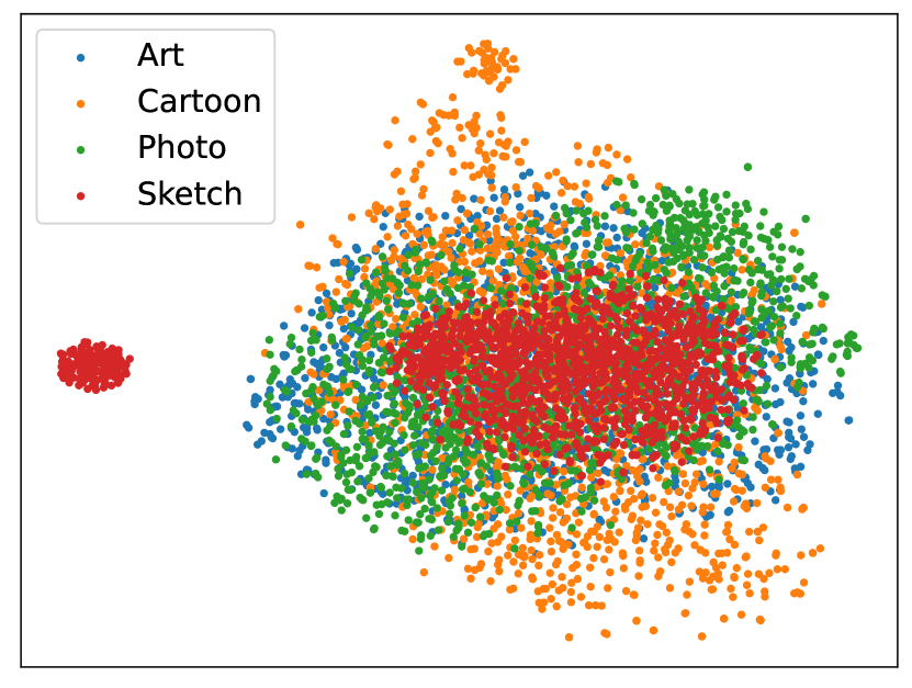
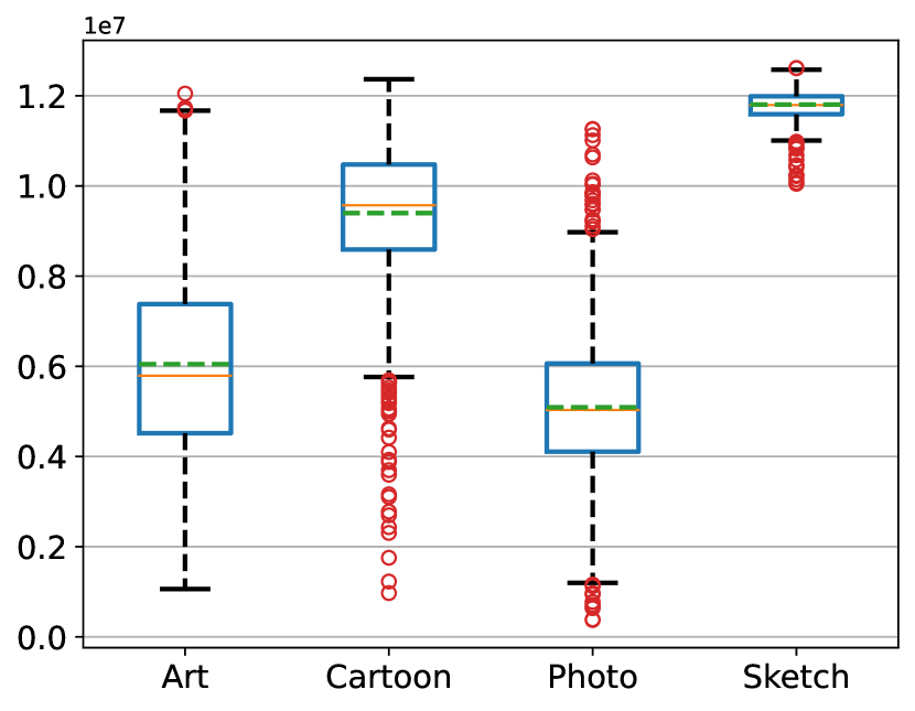
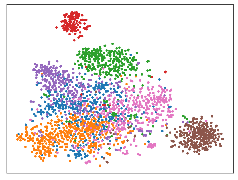
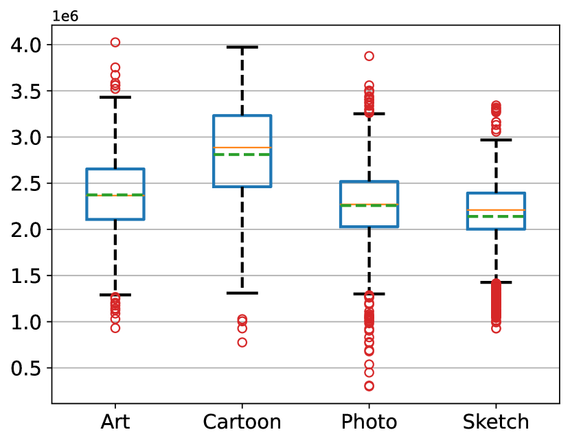
Due to the well-known property of the Fourier transform, that the phase spectrum preserves high-level semantics of the image while the amplitude spectrum contains low-level statistics [16, 40, 41, 58], recent studies [5, 14, 32, 48, 53] have focused on exploring the explanations for CNN’s generalizability in the frequency domain. Experiments conducted in these studies have demonstrated the sensitivity of CNNs to the amplitude spectrum. To visually explore the relationships between the amplitude spectrum and domain shifts, we randomly select 1500 images from each domain in PACS [28] and present the t-SNE [51] distribution of their amplitude spectra in Fig. 1(b). Additionally, we calculate the centroid frequency $F_{c}$ and frequency standard deviation $F_{std}$ for the amplitude spectra. The amplitude spectra of Art Painting and Photo show a substantial overlap. In contrast, Cartoon and Sketch exhibit significant domain shifts, resulting in numerous outliers and distinct in-domain distributions from Art Painting and Photo. These observations align with the statistics presented in Figs. 1(c) and 1(d), where the two statistics of Cartoon and Sketch significantly differ from the others.

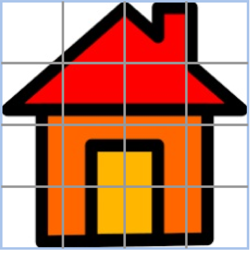
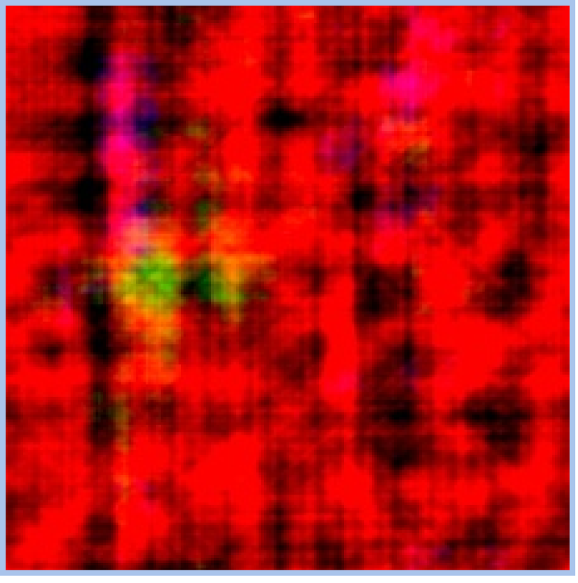
For the phase spectrum, we conduct an empirical experiment following the approach in [57]. Results in Fig. 2 show that the phase spectrum preserves highly structured spatial information, while the amplitude-only reconstructed image is entirely corrupted. Specifically, for each patch in Figs. 2(a) and 2(c), the structural information (e.g., contour, edge) remains remarkably consistent, which makes significant contributions to recognition and positioning for the human visual system. Based on the above observations, we assert that the secret to robust visual systems lies in the utilization of the phase spectrum and low sensitivity to the amplitude spectrum. Moreover, the consistent structural information presented in the image patches motivates us to establish spatial relationships for the phase spectrum. However, existing DG studies have largely overlooked the spatial relationship between the image patches, which is a critical aspect of a generalizable representation.

(a) original image.

(b) amplitude only.

(c) phase only.

Figure 2: Comparison between amplitude-only and phase-only reconstruction.

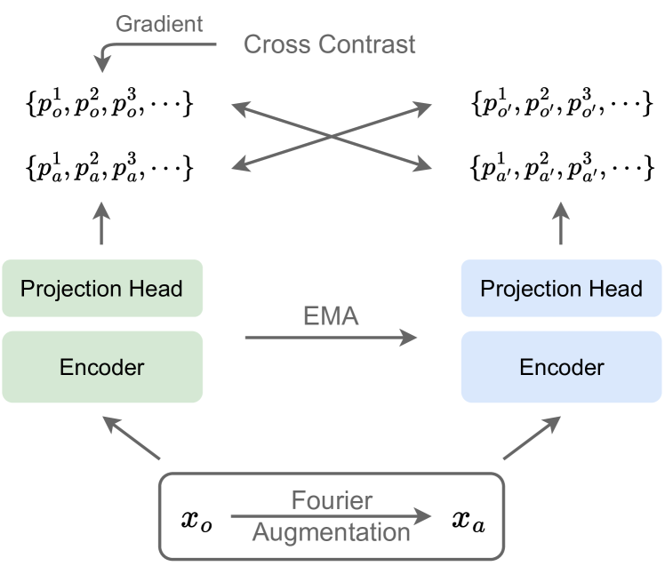
In this paper, we seek to address DG problems from a frequency perspective and propose a method called Phase Matching (PhaMa), as illustrated in Fig. 4. To enhance generalizability against amplitude disturbances caused by domain shifts, we introduce perturbations on the amplitude spectrum for adversarial training. Specifically, we randomly select two images from the source domains and mix their amplitude spectra through linear interpolation. Both the original images and the augmented versions are then fed into the network. Subsequently, we introduce a patch contrastive loss [42] to encourage the matching of patch representations from the image pairs. This operation further alleviates the impact of the amplitude spectrum and establishes the spatial relationship of the phase spectrum, allowing the network to prioritize the phase spectrum of the image.

Our contributions can be summarized as follows: (1) We propose an intuitive causal view for domain generalization using the Fourier transform and specify the causal/non-causal factors associated with the Fourier spectrum. (2) We introduce an effective algorithm called Phase Matching (PhaMa), which guides the network to prioritize the phase spectrum for generalizable representation learning. (3) We provide a new state-of-the-art method on multiple domain generalization benchmarks.

2 Related Work

Domain Generalization. Domain generalization (DG) aims to train a model on source domains that performs well on unseen target domains. Data augmentation is a widely used technique in machine learning to improve the generalization ability of models on out-of-distribution data [54, 65]. MixUP [63] utilizes linear interpolations between two input samples and smooths the label. CutMix [60] generates training images by cutting and pasting from raw images. From the frequency perspective, recent works [5, 57, 33] have incorporated the properties of phase and amplitude of the Fourier spectrum into DG [57, 33] and Robustness [5]. Motivated by the observation that image style can be captured from latent feature statistics [50, 22], many DG methods utilize adaptive instance normalization (AdaIN) [22] and its variants [38, 68, 31] to synthesize novel feature statistics. Another way to tackle DG problems is domain-invariant representation learning. For example, MMD-AAE [29] regularizes a multi-domain autoencoder by minimizing the Maximum Mean Discrepancy (MMD) distance. [64] minimizes the KL divergence between the conditional distributions of different training domains. DAL [43] disentangles domain-specific features using adversarial losses.

CNN Behaviors from Frequency Perspective. Several frequency-based researches on CNN have beeen conducted. [14] conducts adversarial attacks on low-frequency components and reveals that CNN primarily utilizes the low-frequency components for prediction. [48] demonstrates that CNN is vulnerable under low-frequency perturbations. On the other hand, [53] observes that high-frequency components are essential for the generalization of CNN. Further, APR [5] provides a qualitative study for both the amplitude and phase spectrum, and argues that the phase spectrum is crucial for robust recognition. However, the spatial relationships of the phase spectrum remain unexplored, which we aim to investigate from a contrastive view.

Contrastive Learning. As a simple and powerful tool for visual representation learning, there has been a surge of impressive studies [4, 6, 17, 55] on contrastive learning [15]. InstDisc [55] uses a memory-bank to store the features for contrast. MoCo [17] builds a dictionary with a quene and a momentum upadte encoder. SimCLR [6] introduces a learnable projection head between encoder networks and the contrastive loss. DINO [4] trains the Vision Transformer (ViT) [9] using contrastive learning, and gets explicit semantic information.

Given that contrastive learning only requires a definition of positive-negative pairs, it has recently been introduced into DG. PDEN [30] and SelfReg [25] aligns the cross-domain positive pairs by contrastive learning. PCL [59] proposes a proxy-based contrast method for DG.

3 Method

In this section, we provide a comprehensive explanation for the causal relationships between domain generalization and the Fourier components. We demonstrate that the phase spectrum plays a significant role in cross-domain representation, while the amplitude spectrum serves as a redundant visual signal for DG. Hence, we propose to learn the intrinsic representation from the phase spectrum, while maintaining robustness to amplitude perturbations.

3.1 Problem Definition

Given a training set consisting of $M$ source domains $\mathcal{D}_{s}=\left\{\mathcal{D}_{k}|k=1,\dots,M\right\}$ where $\mathcal{D}_{k}=\{(x_{l}^{k},y_{l}^{k})\}_{l=1}^{n_{k}}$ denotes the $k$-th domain. The goal of domain generalization is to learn a robust and generalizable model $g:\mathcal{X}\to\mathcal{Y}$ from the $M$ source domains and achieve a minimum prediction error on the traget domain $\mathcal{D}_{t}$, which is inaccessible during training:

$$\min_{g}\mathbb{E}_{(x,y)\in\mathcal{D}_{t}}\left[\ell(g(x),y)\right].$$ (1)

In this paper, we consider an object recognition model $g(\cdot;\theta):\mathcal{X}\to\mathbb{R}^{N}$, where $\theta$ denotes the model parameters, $N$ is the number of catrgories in the target domain.

3.2 A Frequency Causal View for DG

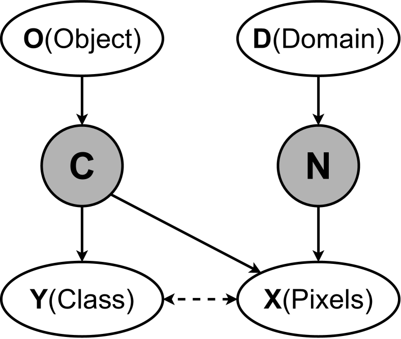
To gain deeper insights into the relationship between the Fourier spectra and DG, we initially consider domain generalization as a domain-specific image generation task from a causal perspective. As depicted in Fig. 3(a), given information about an object (O) and a domain (D), the pixels of the image $X$ are constructed with both the latent embeddings of object and domain, whereas the category $Y$ is solely influenced by object. In this context, we consider the latent embeddings caused by object and domain as causal factors (C) and non-causal factors (N), respectively.

Based on Reichenbach’s Common Cause Principle [45], the Structural Causal Model (SCM) of the domain-specific image generation process can be formulated as follows:

$$C =U_{O},N=U_{D},$$ (2)

$$X =g_{x}(C,N;\theta)+U_{X},$$

$$Y =g_{y}(C;\theta)+U_{Y},$$

where $U=\{U_{O},U_{D},U_{X},U_{Y}\}$ denotes the exogenous variables, and $V=\{X,Y,C,N\}$ denotes the endogenous variables. Note that $C$ and $N$ satisfy the following conditions: (1) $C\not\!\perp\!\!\!\perp O$, $N\not\!\perp\!\!\!\perp D$; (2) $C\perp\!\!\!\perp D\mid O$, $N\perp\!\!\!\perp O\mid D$. The latter condition ensures that $C$ is invariant with the same object across different domains, and $N$ is independent of the object. Unfortunately, due to the unobservation of causal/non-causal factors, we cannot directly formulate $X=g_{x}(C,N;\theta)+U_{X}$, which remains a challenging problem for causal inference [12] and poses a further obstacle to modeling the distribution from $X$ to $Y$.

(a) General form.

(b) Specified form.

Figure 3: Structural causal models (SCMs) for DG. The solid arrow denotes the parent node causes the child node; the dash arrow denotes correlation; shaded variables are unobserved.

Based on the observations in Sec. 1, we believe that introducing the Fourier transform into causal inference might help learn causal representations. Hence, with reference to [5, 34], we make the following assumption for components of the Fourier transform:

Assumption 1

The phase component of the Fourier spectrum is dependent on both the object and domain information. The amplitude component is only dependent on the domain information.

With Assumption 1, we can have a formal statement for the generation process:

Corollary 1

The category of the generated image is only dependent on the phase spectrum, the pixels of the image are constructed from both the phase and amplitude spectrum.

The proof is omitted because Corollary 1 has been empirically verified in Sec. 1 and previous work [5]. Therefore, the corollary can serve as the causal explanation for the generalizability of CNN in DG.

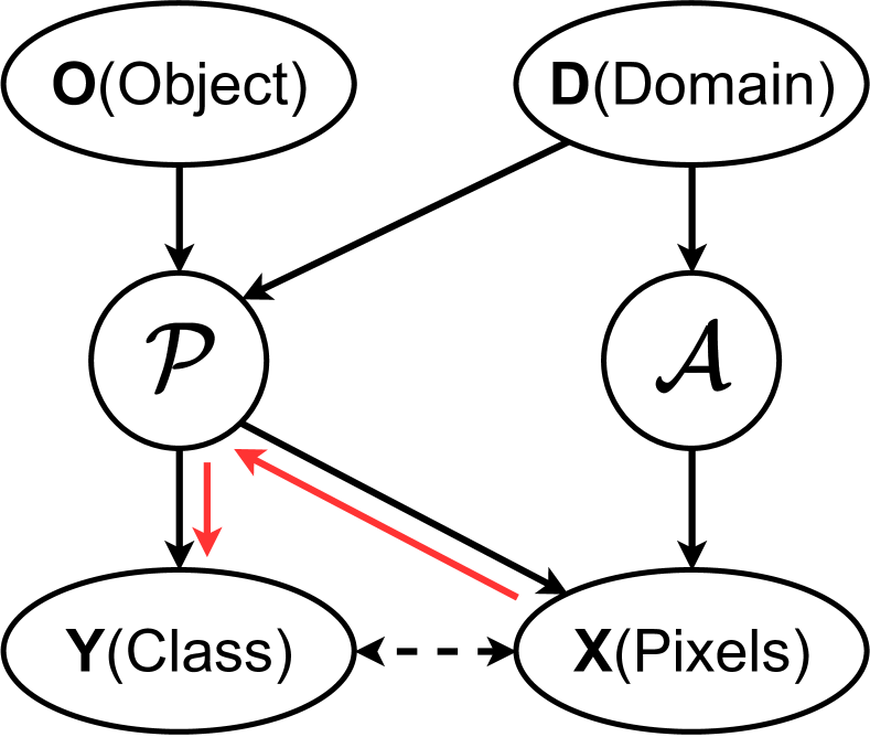
With Corollary 1, we treat the phase spectrum $\mathcal{P}$ as the semi-causal factors (note that a causal relation between domain (D) and the phase spectrum ($\mathcal{P}$) is introduced) and the amplitude spectrum $\mathcal{A}$ as the redundant non-causal factors. We transform the general SCM (Eq. 2) into the following specified form (Fig. 3(b)):

$$\mathcal{P} =U_{O}+U_{D},\mathcal{A}=U_{D},$$ (3)

$$X =g_{x}(\mathcal{P},\mathcal{A};\theta)+U_{X},$$

$$Y =g_{y}(\mathcal{P};\theta)+U_{Y}.$$

Therefore, our objective is to learn the mapping of $Y$ as $g(X_{\mathcal{P}};\theta)$, where $g:\mathcal{X}\to\mathbb{R}^{N}$ and $X_{\mathcal{P}}$ represents the phase spectrum of input signal $X$. This process is illustrated by the red arrows in Fig. 3(b).

Here, we present an intuitive view of the SCM of DG from the frequency perspective. By having access to the factors in causal inference, we can perform operations on the specified factors instead of blindly exploring the highly-entangled latent space. As the amplitude spectrum has no association with the category, reducing its impact can significantly improve the Signal-to-Noise Ratio (SNR) of the image, thereby aiding the model in learning the intrinsic features of objects from the phase spectrum.

3.3 Phase Matching

From the above perspective, domain generalization can be viewed as a process of generating domain-specific images, where the phase spectrum of the image is considered as the semi-causal factors. Our hypothesis is that a robust representation remains invariant to the phase spectrum of the object despite significant perturbations in the amplitude spectrum. Based on this motivation, we present Phase Matching as described next.

3.3.1 Amplitude Perturbation Data Augmentation

As is discussed in Secs. 1 and 3.2, the amplitude spectrum usually has huge variations under domain shifts. To make the network robust to this perturbation, an intuitive way is to add attacks for the training examples to get adversarial gradients. Therefore, we introduce perturbations by linearly interpolating between the amplitude spectra of two randomly-sampled images, while maintaining the phase spectra unchanged as in [57, 33].

Formally, given an image $x\in\mathbb{R}^{H\times W\times 3}$, we can obtain the complex spectrum $\mathcal{F}\in\mathbb{C}^{H\times W\times 3}$ computed across the spatial dimension within each channel using FFT [39]:

$$\mathcal{F}(x)(u,v)=\sum_{h=0}^{H-1}\sum_{w=0}^{W-1}x(h,w)\cdot e^{-j2\pi(\frac{h}{H}u+\frac{w}{W}v)},$$ (4)

where $H$ and $W$ represent the height and width of the image respectively.

We then perturb the amplitude spectra of two images $x_{o}$ and $x_{o}^{\prime}$, which are randomly selected from source domains, in the same way as MixUP [63]:

$$\hat{\mathcal{A}}_{o}^{o^{\prime}}=(1-\lambda)\mathcal{A}\left(x_{o}\right)+\lambda\mathcal{A}\left(x_{o}^{\prime}\right),$$ (5)

where $\lambda\sim U(0,\eta)$ and $\eta$ is a hyperparameter that controls the scale of perturbation. The phase-invariant image $x_{a}$ is then reconstructed from the combination of the original phase component and mixed amplitude component:

$$x_{a}=\mathcal{F}^{-1}(\hat{\mathcal{A}}_{o}^{o^{\prime}}\otimes e^{-j\cdot\mathcal{P}(x_{o})}).$$ (6)

The image pairs and the corresponding original labels are both fed to the model for training. The prediction loss is formulated as the standard Cross Entropy Loss:

$$\mathcal{L}^{o(a)}_{cls}=-y^{T}\log(prob(x_{o(a)})),$$ (7)

where $prob$ denotes the probability of each category.

By utilizing this simple operation, we enhance the network’s robustness against unknown amplitude shifts. More importantly, since the phase spectrum remains intact during this operation, we effectively create positive pairs, which paves the way for our subsequent contrastive regularization. This regularization further enhances the network’s ability to capture phase spectrum features.

Figure 4: Framework of PhaMa. The Fourier-augmented image pairs ($x_{o}$ and $x_{a}$) are both fed to the encoder and the momentum-updated encoder. Then, the last-two-level features are sent to a 2-layer nonlinear projection head for extracting patch representations $p_{o(a)}^{i}$. The cross-contrastive gradients are backpropagated for updating the encoder and projection head (in green); for the momentums (in blue), parameters are updated using EMA.

3.3.2 Matching Phase with Cross Patch Contrast

At the core of our method is matching the phase spectrum of the original image with the corresponding augmented image; in other words, the representation of the image pairs should exhibit similarity or even be the same. Our research reveals that there is currently no neural network-based method that specifically focuses on extracting phase spectrum features. Consequently, we face challenges in directly matching the phase embeddings with common metrics such as L1, L2, and KLD. To address this, we incorporate contrastive learning [15], an unsupervised learning method that measures the similarities of sample pairs in a representation space, into our method.

Given the encoded hierarchal feature maps of an image $f_{t}(x)$, where $t$ denotes the index of the feature map, e.g., for a ResNet-like network, $t\in\left\{1,2,3,4\right\}$. Our choice of the feature representations is the last-two-levels in a hierarchal network, in that the high-level features of the network are more likely to extract semantic-related information [62]. Specifically, for the two hierarchal representations $f_{3}\in\mathbb{R}^{C_{3}\times H_{3}\times W_{3}}$ and $f_{4}\in\mathbb{R}^{C_{4}\times H_{4}\times W_{4}}$, we resize $f_{4}$ using bilinear interpolation and concatenate them in the channel dimension, denoted as $z$, and send them to a 2-layer nonlinear projection head $p(z)=W^{(1)}\sigma(W^{(2)}z)$ as in [6], where $\sigma$ denotes the ReLU activation function.

Inspired by the high consistency of the phase spectrum in preserving spatial structures, i.e., for the same position in the image pairs in Sec. 1, contours and edges are highly consistent. We aim to establish associations for each patch in the spatial dimension, i.e., make the patch representations from the same location similar, and push away those from different positions as far as possible. In this way, the encoded representations from each patch are consistent under the amplitude perturbations, and the network can learn from the invariant phase spectrum. Therefore, the following PatchNCE loss [42] is considered:

$$\mathcal{L}_{patch}^{o2a^{\prime}}=-\sum_{i}\log\frac{\exp\left(p^{o}_{i}\cdot p^{a^{\prime}}_{i}/\tau\right)}{\exp\left(p^{o}_{i}\cdot p^{a^{\prime}}_{i}/\tau\right)+\sum_{j}\exp\left(p^{o}_{i}\cdot p^{a^{\prime}}_{j}/\tau\right)},$$ (8)

where $p^{o}$ and $p^{a^{\prime}}$ are from the network (in green) and the momentum network (in blue), respectively. $i(j)\in\left\{1,\ldots,P\right\}$ denotes the index of the patch, and $\left(\cdot\right)$ denotes the innear product. $\tau$ is a temperature parameter. For the $i$-th patch in the original image $p^{o}_{i}$, patches in other locations in the augmented image $p^{a^{\prime}}_{j}(j\neq i)$ are treated as negative samples. The contrast can then be set as a $P$-way classification problem (Fig. 5).

However, existing pre-trained networks [18, 9] extract significantly different representations under huge perturbations of the amplitude spectrum, which tends to cause gradient collapse during the back-propagation in our experiments (Sec. 4.3). To alleviate the impact caused by amplitude perturbations, we propose the following two techniques:

• For both the original and augmented images, we adopt a momentum-updated rule to ensure consistent representation extraction, following the approach proposed in [17]. Specifically, we update the parameters of the network ($\theta_{n}$), and the momentum network’s $\theta_{m}$, using the following rule:

  $$\theta_{m}\leftarrow m\theta_{m}+(1-m)\theta_{n}.$$ (9)

• We perform the patch contrast operation (Eq. 8) across the patch representation of the original image and the augmented image from the network and the momentum network, respectively. The cross-contrastive loss is defined as:

  $$\mathcal{L}_{contr}=\mathcal{L}_{patch}^{o2a^{\prime}}+\mathcal{L}_{patch}^{a2o^{\prime}}.$$ (10)

Figure 5: Illustration of PatchNCE loss.

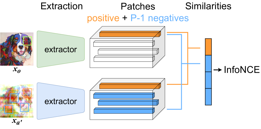
The overall objective function of our proposed method can be formulated as follows:

$$\mathcal{L}_{PhaMa}=\frac{1}{2}(\mathcal{L}_{cls}^{o}+\mathcal{L}_{cls}^{a})+\beta\mathcal{L}_{contr},$$ (11)

where $\beta$ is a trade-off parameter.

4 Experiments

In this section, we perform experiments on various benchmarks to assess the effectiveness of our method in enhancing the network’s generalization capabilities. The evaluation includes multi-domain classification and robustness against corruptions. We also provide ablation studies and visualization to better illustrate how our model operates and the extent of its impact.

4.1 Multi-domain Classification

4.1.1 Implementation Details

Datasets. We evaluate the generalization ability of our method on the following 3 datasets: (1) Digits-DG [66] consists of four datasets MNIST [27], MNIST-M [11], SVHN [37], SYN [11]; (2) PACS [28] is a commonly used benchmark for domain generalization, comprising of 9991 images from four distinct domains: Art Painting, Cartoon, Photo, Sketch; (3) Office-Home [52] contains around 15,500 images of 65 categories from four domains: Artistic, Clipart, Product and Real World.

Training. For all DG benchmarks, we follow the leave-one-domain-out protocol with the official train-val split and report the classification accuracy (%) on the entire held-out target domain. We also use standard augmentation, which consists of random resized cropping, horizontal flipping, and color jittering. For Digits-DG, all images are resized to $32\times 32$. We train the encoder (same as in [66]) from scratch using SGD, batch size 64, and weight decay of 5e-4. The learning rate is initially 0.05 and is decayed by 0.1 every 20 epochs. For PACS and Office-Home, all images are resized to $224\times 224$. We use the ImageNet pretrained ResNet [18] as the encoder and train the network with SGD, batch size 64, momentum 0.9, and weight decay 5e-4 for 50 epochs. The initial learning rate is 0.001 and is decayed by 0.1 at 80% of the total epochs.

Method-specific. We use a sigmoid ramp-up [49] for $\beta$ within the first 5 epochs in all experiments in this section. The scale parameter $\eta$ is set to 1.0 for Digits-DG and PACS, 0.2 for Office-Home. The trade-off parameter $\beta$ is set to 0.1 for Digits-DG and 0.5 for PACS and Office-Home. The momentum $m$ is set to 0.9995. We also follow the common setting [55] to let $\tau=0.07$.

Model Selection. We use training-domain validation set for model selection. Specifically, we train our model on the training splits of all source domains and choose the model maximizing the accuracy on the overall validation set.

4.1.2 Results Analysis

Method	MNIST	MNIST-M	SVHN	SYN	Avg.
Baseline	95.8	58.8	61.7	78.6	73.7
CCSA [35]	95.2	58.2	65.5	79.1	74.5
MMD-AAE [29]	96.5	58.4	65.0	78.4	74.6
CrossGrad [47]	96.7	61.1	65.3	80.2	75.8
DDAIG [66]	96.6	64.1	68.6	81.0	77.6
Jigen [3]	96.5	61.4	63.7	74.0	73.9
L2A-OT [67]	96.7	63.9	68.6	83.2	78.1
MixStyle [68]	96.5	63.5	64.7	81.2	76.5
FACT [57]	96.8	63.2	73.6	89.3	80.7
PhaMa (ours)	97.3	63.9	73.2	90.2	81.1

Table 1: Leave-one-domain-out classification accuracy (%) on Digits-DG with ConvNet in [66].

Method	Art	Cartoon	Photo	Sketch	Avg.
ResNet-18
Baseline	77.6	76.7	95.8	69.5	79.9
MixUP [63]	76.8	74.9	95.8	66.6	78.5
CutMix [60]	74.6	71.8	95.6	65.3	76.8
pAdaIN [38]	81.7	76.6	96.3	75.1	82.5
MixStyle [68]	82.3	79.0	96.3	73.8	82.8
DSU [31]	83.6	79.6	95.8	77.6	84.1
MetaReg [2]	83.7	77.2	95.5	70.3	81.7
JiGen [3]	79.4	75.2	96.0	71.3	80.5
MASF [10]	80.2	77.1	94.9	71.6	81.1
L2A-OT [67]	83.3	78.0	96.2	73.6	82.8
RSC${\ddagger}$  [23]	80.5	78.6	94.4	76.0	82.4
MatchDG [34]	81.3	80.7	96.5	79.7	84.5
SelfReg [25]	82.3	78.4	96.2	77.4	83.6
FACT [57]	85.3	78.3	95.1	79.1	84.5
PhaMa (ours)	84.8	79.1	96.6	79.7	85.1
ResNet-50
Baseline	84.9	76.9	97.6	76.7	84.1
MetaReg [2]	87.2	79.2	97.6	70.3	83.6
MASF [10]	82.8	80.4	95.0	72.2	82.7
RSC${\ddagger}$  [23]	83.9	79.5	95.1	82.2	85.2
MatchDG [34]	85.6	82.1	97.9	78.7	86.1
FACT [57]	89.6	81.7	96.7	84.4	88.1
PhaMa (ours)	89.6	82.7	97.2	83.7	88.3

Table 2: Leave-one-domain-out classification accuracy (%) on PACS with ResNet pretrained on ImageNet. ${\ddagger}$ denotes the reproduced results from FACT [57].

Method	Art	Clipart	Product	Real	Avg.
Baseline	57.8	52.7	73.5	74.8	64.7
CCSA [35]	59.9	49.9	74.1	75.7	64.9
MMD-AAE [29]	56.5	47.3	72.1	74.8	62.7
CrossGrad [47]	58.4	49.4	73.9	75.8	64.4
DDAIG [66]	59.2	52.3	74.6	76.0	65.5
L2A-OT [67]	60.6	50.1	74.8	77.0	65.6
Jigen [3]	53.0	47.5	71.4	72.7	61.2
MixStyle [68]	58.7	53.4	74.2	75.9	65.5
DSU [31]	60.2	54.8	74.1	75.1	66.1
FACT [57]	60.3	54.8	74.4	76.5	66.5
PhaMa (ours)	60.2	54.0	75.2	76.4	66.5

Table 3: Leave-one-domain-out classification accuracy (%) on Office-Home with ResNet-18 pretrained on ImageNet.

Digits-DG. Results are shown in Tab. 1. PhaMa achieves significant improvement over the baseline method and surpasses previous domain-invariant methods by a large margin. Since our method adopts the same augmentation technique as FACT [57], we compare our method with it. Our method shows slight improvement over FACT, indicating that matching the patch feature is more suitable for cross-domain representation.

PACS. The experimental results presented in Tab. 2 show a significant improvement of PhaMa compared to the baseline approach. Particularly, PhaMa exhibits substantial improvements in average accuracy, notably in the Art, Cartoon, and Sketch domains. It is worth noting that previous DG methods experience a slight drop in accuracy for the Photo domain, which shares similar domain characteristics with the ImageNet dataset, and this drop might be attributed to ImageNet pretraining. However, our method is capable of maintaining, or even improving the performance in the Photo domain, demonstrating that contrasting phase components does not degrade raw representations.

Note that other contrast-based methods (e.g., MatchDG and SelfReg) also demonstrate competitive performance on Photo and other domains. This observation highlights the effectiveness of contrastive learning as a powerful tool for DG. Meanwhile, the exceptional performance of PhaMa suggests that introducing spatial contrast for the phase spectrum can yield promising results.

Office-Home. Results are shown in Tab. 3. It can be observed that our method brings obvious improvement over the baseline method and also achieves competitive results against FACT. By introducing amplitude perturbations and the patch contrastive loss, the model can learn to alleviate the amplitude impacts and focus on the phase spectrum.

4.2 Robustness Against Corruptions

4.2.1 Implementation Details

Method	ResNet	DenseNet	WideResNet	ResNeXt
CIFAR-10-C
Standard	-	30.7	26.9	27.5
Cutout [8]	-	32.1	26.8	28.9
MixUP [63]	-	24.6	22.3	22.6
CutMix [60]	-	33.5	27.1	29.5
Adv Training	-	27.6	26.2	27.0
APR [5]	16.7	20.3	18.3	18.5
PhaMa (ours)	17.5	20.3	17.5	17.9
CIFAR-100-C
Standard	-	59.3	53.3	53.4
Cutout [8]	-	59.6	53.5	54.6
MixUP [63]	-	55.4	50.4	51.4
CutMix [60]	-	59.2	52.9	54.1
Adv Training	-	55.2	55.1	54.4
APR [5]	43.8	49.8	44.7	44.2
PhaMa (ours)	43.8	48.5	43.9	41.5

Table 4: Mean Corruption Error (%) on CIFAR-10(100)-C.

Datasets. We evaluate the robustness against corruptions of our method on CIFAR-10-C, CIFAR-100-C [19]. The two datasets are constructed by corrupting the test split of original CIFAR datasets with a total of 15 corruption types (noise, blur, weather, and digital). Note that the 15 corruptions are not introduced during training.

Training. Following [5], we report the mean Corruption Error (%) for various networks, including ResNet-18 [18], 40-2 Wide-ResNet [61], DenseNet-BC ($k=2,d=100$) [21], and ResNeXt-29 ($32\times 4$) [56]. All networks use an initial learning rate of 0.1 which decay every 60 epochs. We train all models from scratch for 200 epochs using SGD, batch size 128, momentum 0.9. All input images are randomly processed with resized cropping and horizontal flipping.

Method-specific. All configurations are consistant with Sec. 4.1.1 except for the sigmoid ramp-up.

Model Selection. We select the last-epoch checkpoint for evaluations on corrupted datasets.

4.2.2 Results Analysis

Results on CIFAR-10-C and CIFAR-100-C are shown in Tab. 4. PhaMa outperforms conventional data augmentation techniques (Cutout, MixUP, CutMix) by a significant margin. Furthermore, PhaMa shows slight improvements over APR, which also employs a technique similar to ours in the frequency domain. This observation further highlights the significance of establishing spatial relationships within the phase spectrum, leading to a more effective extraction of intrinsic representations.

4.3 Ablation Studies

Method	APDA	$\mathcal{L}_{patch}^{o2a}$	$\mathcal{L}_{patch}^{a2o}$	MoEnc	Art	Cartoon	Photo	Sketch	Avg.
Baseline	-	-	-	-	77.6	76.7	95.8	69.5	79.9
Variant A	✓	-	-	-	83.9	76.9	95.5	77.6	83.4
Variant B	✓	✓	✓	-	83.2	77.1	95.5	79.0	83.7
Variant C	✓	✓	-	✓	84.2	78.7	96.1	79.5	84.6
Variant D	✓	-	✓	✓	84.1	78.4	95.5	79.1	84.5
PhaMa	✓	✓	✓	✓	84.8	79.1	96.6	79.7	85.1

Table 5: Effects of different modules on PACS with ResNet-18.

Effects of Different Modules. We conduct ablation studies to investigate the impact of each module in our method in Tab. 5. Compared with baseline, the amplitude perturbation data augmentation module (APDA) plays a significant role in our method, lifting the performance by a margin of 4.5%. We exclude the momentum-updated encoder (MoEnc) for variant B, and the performance drops by nearly 1%, demonstrating the over-dependence on the amplitude spectrum makes the feature extraction inefficient. With the cross-contrast operation for the image pairs, PhaMa surpasses variant C and D, suggesting that keeping the consistency between the image pairs is important for the training of contrastive learning.

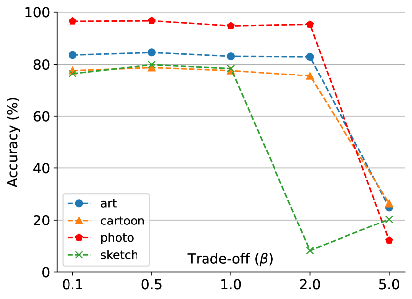
Sensitivity of Trade-off Parameter. The hyperparameter $\beta$ controls the trade-off between the classification loss and the patch contrastive loss. We experiment with different values of $\beta$ from the set $\left\{0.1,0.5,1.0,2.0,5.0\right\}$. The results, depicted in Fig. 6, show that for small $\beta$ values, there are slight oscillations. However, when $\beta$ is set to a large value, the training process collapses. The collapse might be attributed to an over-dependence on the amplitude spectrum of the ImageNet pretrained weights. As $\beta$ increases, the intense contrast may likely corrupt the raw representation.

Figure 6: Evaluation of different trade-off parameters.

Choices of Matching Loss. Since our objective is to match the representation of each patch from the image pairs, we evaluate various types of matching loss, including SmoothL1, MSE, and PatchNCE. As demonstrated in Tab. 6, the PatchNCE loss outperforms the others on Art Painting, Cartoon, and Sketch domains, while also showing competitive performance on the Photo domain. The inferior performance of SmoothL1 and MSE is probably due to the simplistic alignment of the representation, which lacks focus on discriminating the positive patch from the negatives.

Type	Art	Cartoon	Photo	Sketch	Avg.
SmoothL1	83.7	76.6	96.4	72.3	82.3
MSE	81.8	77.4	96.6	76.1	83.0
PatchNCE	84.8	79.1	96.6	79.7	85.1

Table 6: Evaluation of different types of matching loss.

4.4 Visualization

To intuitively present PhaMa’s effects on feature representations, we visualize the feature representation vectors of different categories in the unseen domain using t-SNE [51] in Fig. 7. Compared with the baseline method, features from the same category become more compact with our method. The clustered representations illustrate that our method can alleviate perturbations caused by domain shifts and extract more domain-invariant features.

(a) Baseline.

(b) PhaMa.

Figure 7: t-SNE visualization on Baseline and PhaMa. We visualize the embeddings of ResNet-18 on PACS with Art, Photo and Sketch as the source domains, and Cartoon as the target domain.

5 Discussion and Conclusion

In this paper, we consider Domain Generalization (DG) from a frequency perspective and present PhaMa. The main idea is to establish spatial relationships for the phase spectrum with contrastive learning. Our method shows promising results on many DG benchmarks.

Moreover, several questions are worth rethinking. Although our method alleviates the cross-domain impact of amplitude information, it doesn’t actually build relationships between cross-domain samples, i.e., the intrinsic domain-invariant representation learning is weakly reflected. As shown in Fig. 7, minority features still appear as outliers from the cluster. These limitations might result in the slight improvement of PhaMa on many DG benchmarks. Beyond domain generalization, PhaMa draws on MoCo [17] and SimCLR [6] for many module designs. Considering the great property of the Fourier transform, it is worth thinking that whether the Fourier transform and the spatial relationships of the phase spectrum can be extended to unsupervised visual representation learning or even multimodal learning [44]. We hope our work can bring more inspirations into the community.

6 Appendix

6.1 Analysis of the Amplitude Spectrum for Cross-Domain Samples

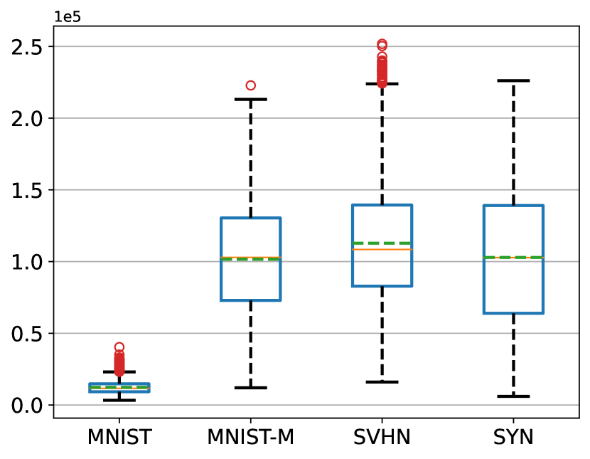
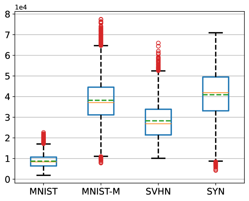
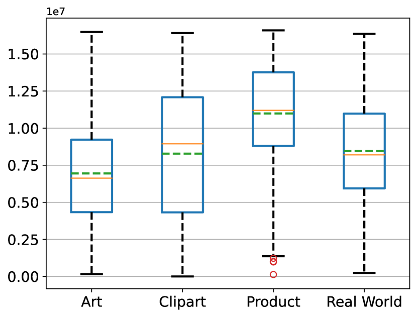
In this section, we first provide the definition of two commonly used frequency domain statistics and present the results on the amplitude spectra from PACS [28], Digits-DG [66], Office-Home [52] and CIFAR-10(100)(-C) [19].

6.1.1 Mathematical Definition

To obtain the statistical features of the amplitude spectra, we calculate two commonly-used frequency statistics for the amplitude spectra of the selected samples.

Centroid Frequency represents the center or balance point of the signal energy, which is the weighted average of the spectrum. In our experiments, it can be defined as:

$$F_{c}=\frac{\sum{X_{i}\cdot X_{i}^{2}}}{\sum{X_{i}^{2}}},$$ (12)

where $X_{i}$ denotes the amplitude of the $i$-th frequency component.

Frequency Standard Deviation is a statistical measure used in the frequency domain to quantify the breadth or dispersion of signal frequency distribution, which can be formulated as:

$$F_{std}=\sqrt{\frac{\sum{(X_{i}-F_{c})^{2}\cdot X_{i}^{2}}}{\sum{X_{i}^{2}}}}.$$ (13)

6.1.2 Comparison on DG Benchmarks

PACS. We randomly select 1500 images from each domain in PACS, and calculate the in-domain centroid frequency $F_{c}$ and frequency standard deviation $F_{std}$ for the amplitude spectra. As shown in Fig. 8, it is clear that each domain’s amplitude spectra exhibit a distinct distribution. For Art Painting and Photo, their distributions are similar, whereas Cartoon and Sketch show significant statistical differences. These results support the observations made in the Introduction and further reinforce the susceptibility of the amplitude spectrum to domain shifts.

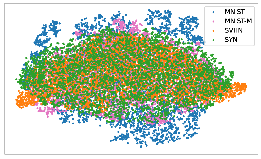
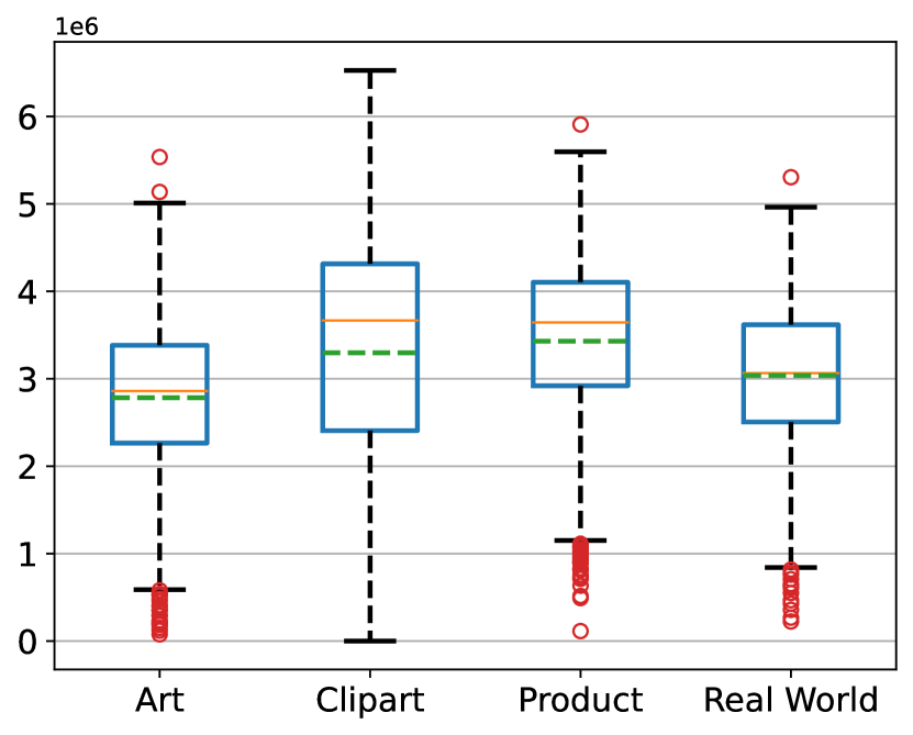
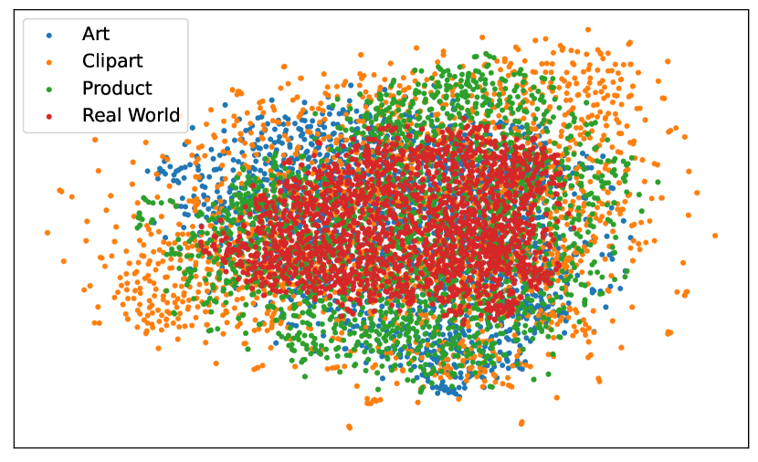
Digits-DG & Office-Home. We randomly select 5000 images from each domain in Digits-DG and 2000 images from each domain in Office-Home. The frequency statistics and t-SNE [51] visualization are presented in Figs. 9 and 10.

(a) $F_{c}$.

(b) $F_{std}$.

Figure 8: Boxplots of centroid frequency and frequency standard deviation of the amplitude spectra from PACS.

(a) $F_{c}$.

(b) $F_{std}$.

(c) t-SNE.

Figure 9: (a) and (b) are the boxplots of centroid frequency and frequency standard deviation of the amplitude spectra from Digits-DG. (c) is the t-SNE visualization of the amplitude spectra.

(a) $F_{c}$.

(b) $F_{std}$.

(c) t-SNE.

Figure 10: (a) and (b) are the boxplots of centroid frequency and frequency standard deviation of the amplitude spectra from Office-Home. (c) is the t-SNE visualization of the amplitude spectra.

6.1.3 Comparison on CIFAR-10(100)(-C)

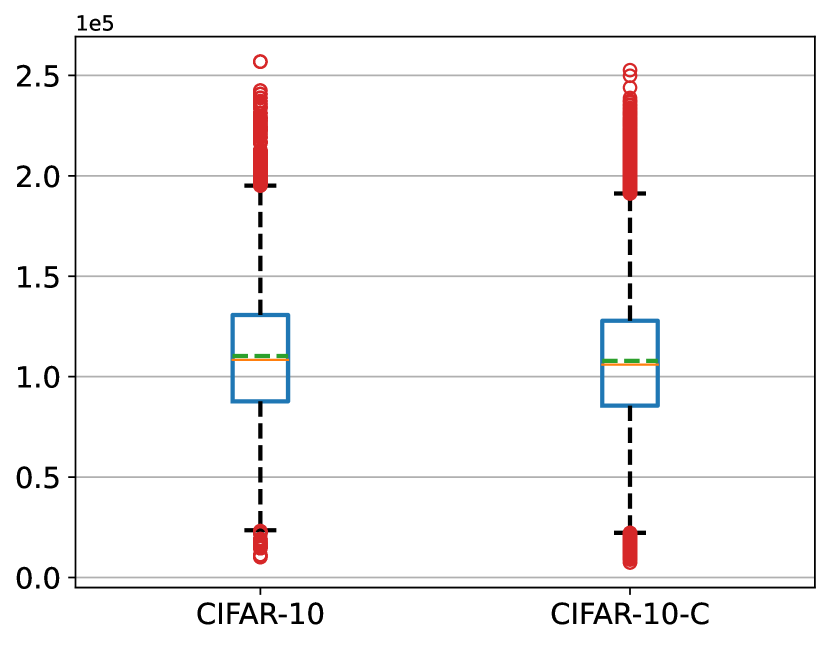
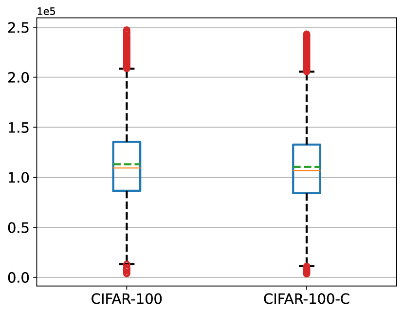
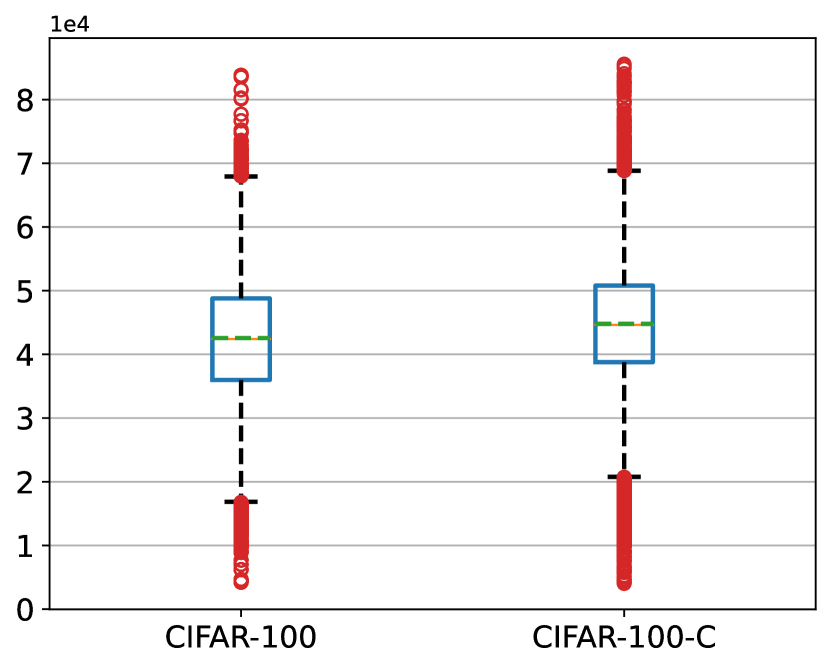
We randomly select 50000 images from the test split of CIFAR-10(100) (15 copies) and CIFAR-10(100)-C, respectively. The presented statistics in Fig. 11 further demonstrate the amplitude spectrum’s sensitivity to domain shifts.

(a) $F_{c}$.

(b) $F_{std}$.

(c) $F_{c}$.

(d) $F_{std}$.

Figure 11: Boxplots of the centroid frequency and frequency standard deviation of the amplitude spectra on CIFAR(-C).

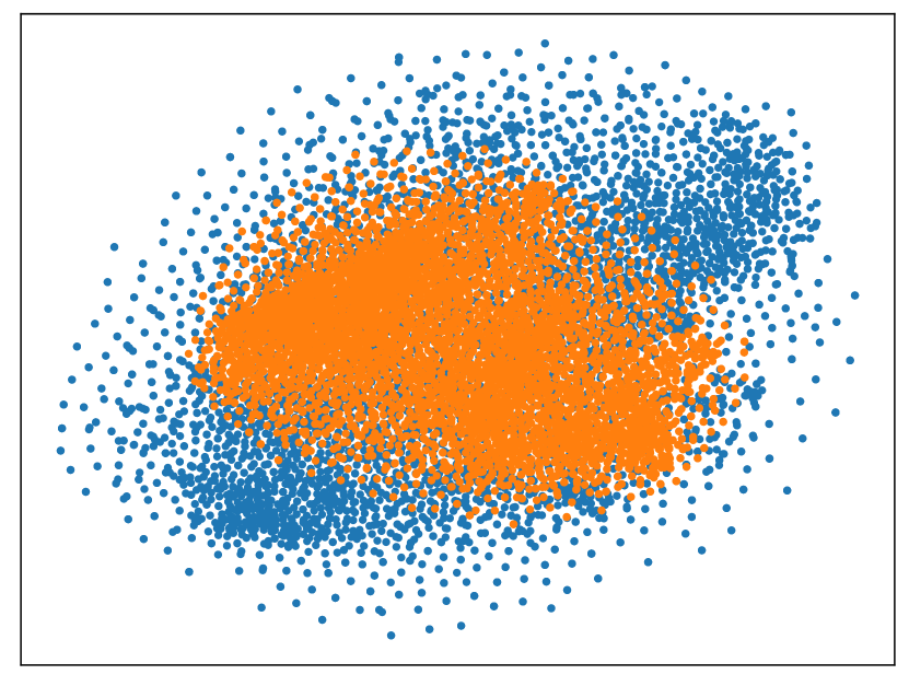
Additionally, we provide the t-SNE visualization of the amplitude spectra on CIFAR(-C) in Fig. 12. The corrupted samples exhibit a notably distinct t-SNE distribution compared to the original samples.

(a) CIFAR-10(-C).

(b) CIFAR-100(-C).

Figure 12: t-SNE visualization of CIFAR-10(100) (blue) and CIFAR-10(100)-C (orange).

6.2 Extra Ablation Studies

Impacts of Hierarchies. Table 7 compares different hierarchical positions (indexed with 1-4) in the ResNet bolcks for contrastive learning. As can be seen, the representation extracted from the last two layers occupies the least GPU memory while achieving the best effective performance.

Position	Avg Acc	Mem-Usage
1, 2	82.2	$\approx$43.3
2, 3	83.5	$\approx$12.1
3, 4	85.1	$\approx$11.8

Table 7: Average Accuracy (%) and GPU Memory-Usage (GB) of different posiotions.

6.3 More Examples of Reconstruction

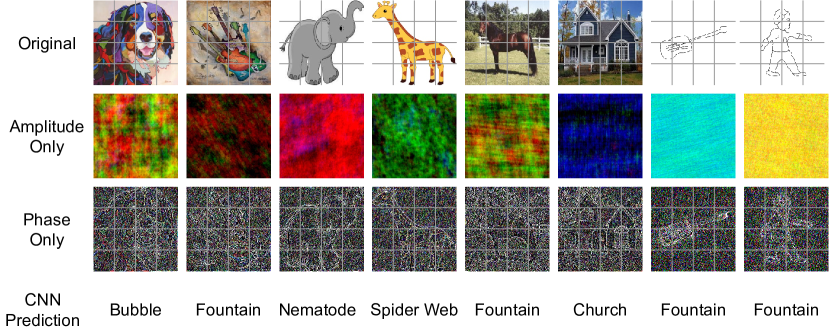
We present more examples of amplitude-only and phase-only reconstructed images, along with the prediction results of ImageNet [7] pretrained ResNet-18 [18]. The preservation of edge and contour information is evident in both the patches of the original images and those of the phase-only reconstructed images. Furthermore, the significant amplitude perturbations corrupt the CNN predictions, indicating the CNN’s excessive reliance on the amplitude spectrum.

Figure 13: Examples of amplitude-only and phase-only reconstruction, with the corresponding CNN prediction of the phase-onlys.

6.4 Attention Maps

To visually verify the claim that the representations learned by PhaMa can prioritize the phase spectrum of the image, we present the attention maps of the baseline method and PhaMa using Grad-CAM [46]. As shown in Fig. 14, the representations learned by PhaMa focus more on category-related information, thus verifying the effectiveness of our method in extracting domain-variant representations.

Figure 14: Visualization of attention maps on PACS.

References

- [1] Martin Arjovsky, Léon Bottou, Ishaan Gulrajani, and David Lopez-Paz. Invariant risk minimization. arXiv:1907.02893, 2019.
- [2] Yogesh Balaji, Swami Sankaranarayanan, and Rama Chellappa. Metareg: Towards domain generalization using meta-regularization. In NeurIPS, 2018.
- [3] Fabio M Carlucci, Antonio D’Innocente, Silvia Bucci, Barbara Caputo, and Tatiana Tommasi. Domain generalization by solving jigsaw puzzles. In CVPR, 2019.
- [4] Mathilde Caron, Hugo Touvron, Ishan Misra, Hervé Jégou, Julien Mairal, Piotr Bojanowski, and Armand Joulin. Emerging properties in self-supervised vision transformers. In ICCV, 2021.
- [5] Guangyao Chen, Peixi Peng, Li Ma, Jia Li, Lin Du, and Yonghong Tian. Amplitude-phase recombination: Rethinking robustness of convolutional neural networks in frequency domain. In ICCV, 2021.
- [6] Ting Chen, Simon Kornblith, Mohammad Norouzi, and Geoffrey Hinton. A simple framework for contrastive learning of visual representations. In ICML, 2020.
- [7] Jia Deng, Wei Dong, Richard Socher, Li-Jia Li, Kai Li, and Li Fei-Fei. Imagenet: A large-scale hierarchical image database. In CVPR, 2009.
- [8] Terrance DeVries and Graham W Taylor. Improved regularization of convolutional neural networks with cutout. arXiv:1708.04552, 2017.
- [9] Alexey Dosovitskiy, Lucas Beyer, Alexander Kolesnikov, Dirk Weissenborn, Xiaohua Zhai, Thomas Unterthiner, Mostafa Dehghani, Matthias Minderer, Georg Heigold, Sylvain Gelly, Jakob Uszkoreit, and Neil Houlsby. An image is worth 16x16 words: Transformers for image recognition at scale. In ICLR, 2021.
- [10] Qi Dou, Daniel Coelho de Castro, Konstantinos Kamnitsas, and Ben Glocker. Domain generalization via model-agnostic learning of semantic features. In NeurIPS, 2019.
- [11] Yaroslav Ganin and Victor Lempitsky. Unsupervised domain adaptation by backpropagation. In ICML, 2015.
- [12] Andrew Gelman. Causality and statistical learning, 2011.
- [13] Ian Goodfellow, Yoshua Bengio, and Aaron Courville. Deep learning. MIT press, 2016.
- [14] Chuan Guo, Jared S Frank, and Kilian Q Weinberger. Low frequency adversarial perturbation. arXiv:1809.08758, 2018.
- [15] Raia Hadsell, Sumit Chopra, and Yann LeCun. Dimensionality reduction by learning an invariant mapping. In CVPR, 2006.
- [16] Bruce C Hansen and Robert F Hess. Structural sparseness and spatial phase alignment in natural scenes. JOSA A, 2007.
- [17] Kaiming He, Haoqi Fan, Yuxin Wu, Saining Xie, and Ross Girshick. Momentum contrast for unsupervised visual representation learning. In CVPR, 2020.
- [18] Kaiming He, Xiangyu Zhang, Shaoqing Ren, and Jian Sun. Deep residual learning for image recognition. In CVPR, 2016.
- [19] Dan Hendrycks and Thomas Dietterich. Benchmarking neural network robustness to common corruptions and perturbations. In ICLR, 2019.
- [20] Dan Hendrycks, Norman Mu, Ekin D Cubuk, Barret Zoph, Justin Gilmer, and Balaji Lakshminarayanan. Augmix: A simple data processing method to improve robustness and uncertainty. In ICLR, 2020.
- [21] Gao Huang, Zhuang Liu, Laurens Van Der Maaten, and Kilian Q Weinberger. Densely connected convolutional networks. In CVPR, 2017.
- [22] Xun Huang and Serge Belongie. Arbitrary style transfer in real-time with adaptive instance normalization. In ICCV, 2017.
- [23] Zeyi Huang, Haohan Wang, Eric P Xing, and Dong Huang. Self-challenging improves cross-domain generalization. In ECCV, 2020.
- [24] Maximilian Ilse, Jakub M Tomczak, Christos Louizos, and Max Welling. Diva: Domain invariant variational autoencoders. In MIDL, 2020.
- [25] Daehee Kim, Youngjun Yoo, Seunghyun Park, Jinkyu Kim, and Jaekoo Lee. Selfreg: Self-supervised contrastive regularization for domain generalization. In ICCV, 2021.
- [26] Yann LeCun, Yoshua Bengio, and Geoffrey Hinton. Deep learning. Nature, 2015.
- [27] Yann LeCun, Léon Bottou, Yoshua Bengio, and Patrick Haffner. Gradient-based learning applied to document recognition. Proceedings of the IEEE, 1998.
- [28] Da Li, Yongxin Yang, Yi-Zhe Song, and Timothy M Hospedales. Deeper, broader and artier domain generalization. In ICCV, 2017.
- [29] Haoliang Li, Sinno Jialin Pan, Shiqi Wang, and Alex C Kot. Domain generalization with adversarial feature learning. In CVPR, 2018.
- [30] Lei Li, Ke Gao, Juan Cao, Ziyao Huang, Yepeng Weng, Xiaoyue Mi, Zhengze Yu, Xiaoya Li, and Boyang Xia. Progressive domain expansion network for single domain generalization. In CVPR, 2021.
- [31] Xiaotong Li, Yongxing Dai, Yixiao Ge, Jun Liu, Ying Shan, and LINGYU DUAN. Uncertainty modeling for out-of-distribution generalization. In ICLR, 2022.
- [32] Honggu Liu, Xiaodan Li, Wenbo Zhou, Yuefeng Chen, Yuan He, Hui Xue, Weiming Zhang, and Nenghai Yu. Spatial-phase shallow learning: rethinking face forgery detection in frequency domain. In CVPR, 2021.
- [33] Fangrui Lv, Jian Liang, Shuang Li, Bin Zang, Chi Harold Liu, Ziteng Wang, and Di Liu. Causality inspired representation learning for domain generalization. In CVPR, 2022.
- [34] Divyat Mahajan, Shruti Tople, and Amit Sharma. Domain generalization using causal matching. In ICML, 2021.
- [35] Saeid Motiian, Marco Piccirilli, Donald A Adjeroh, and Gianfranco Doretto. Unified deep supervised domain adaptation and generalization. In ICCV, 2017.
- [36] Krikamol Muandet, David Balduzzi, and Bernhard Schölkopf. Domain generalization via invariant feature representation. In ICML, 2013.
- [37] Yuval Netzer, Tao Wang, Adam Coates, Alessandro Bissacco, Bo Wu, and Andrew Y Ng. Reading digits in natural images with unsupervised feature learning. 2011.
- [38] Oren Nuriel, Sagie Benaim, and Lior Wolf. Permuted adain: Reducing the bias towards global statistics in image classification. In CVPR, 2021.
- [39] Henri J Nussbaumer. The fast Fourier transform. Springer, 1981.
- [40] A Oppenheim, Jae Lim, Gary Kopec, and SC Pohlig. Phase in speech and pictures. In ICASSP. IEEE, 1979.
- [41] Alan V Oppenheim and Jae S Lim. The importance of phase in signals. Proceedings of the IEEE, 1981.
- [42] Taesung Park, Alexei A Efros, Richard Zhang, and Jun-Yan Zhu. Contrastive learning for unpaired image-to-image translation. In ECCV, 2020.
- [43] Xingchao Peng, Zijun Huang, Ximeng Sun, and Kate Saenko. Domain agnostic learning with disentangled representations. In ICML, 2019.
- [44] Alec Radford, Jong Wook Kim, Chris Hallacy, Aditya Ramesh, Gabriel Goh, Sandhini Agarwal, Girish Sastry, Amanda Askell, Pamela Mishkin, Jack Clark, et al. Learning transferable visual models from natural language supervision. In ICML, 2021.
- [45] Maria Reichenbach and P Morrison. The direction of time. Physics Today, 1956.
- [46] Ramprasaath R Selvaraju, Michael Cogswell, Abhishek Das, Ramakrishna Vedantam, Devi Parikh, and Dhruv Batra. Grad-cam: Visual explanations from deep networks via gradient-based localization. In ICCV.
- [47] Shiv Shankar, Vihari Piratla, Soumen Chakrabarti, Siddhartha Chaudhuri, Preethi Jyothi, and Sunita Sarawagi. Generalizing across domains via cross-gradient training. arXiv:1804.10745, 2018.
- [48] Yash Sharma, Gavin Weiguang Ding, and Marcus Brubaker. On the effectiveness of low frequency perturbations. In IJCAI, 2019.
- [49] Antti Tarvainen and Harri Valpola. Mean teachers are better role models: Weight-averaged consistency targets improve semi-supervised deep learning results. In NeurIPS, 2017.
- [50] Dmitry Ulyanov, Andrea Vedaldi, and Victor Lempitsky. Instance normalization: The missing ingredient for fast stylization. arXiv:1607.08022, 2016.
- [51] Laurens Van der Maaten and Geoffrey Hinton. Visualizing data using t-sne. JMLR, 2008.
- [52] Hemanth Venkateswara, Jose Eusebio, Shayok Chakraborty, and Sethuraman Panchanathan. Deep hashing network for unsupervised domain adaptation. In CVPR, 2017.
- [53] Haohan Wang, Xindi Wu, Zeyi Huang, and Eric P Xing. High-frequency component helps explain the generalization of convolutional neural networks. In CVPR, 2020.
- [54] Jindong Wang, Cuiling Lan, Chang Liu, Yidong Ouyang, Tao Qin, Wang Lu, Yiqiang Chen, Wenjun Zeng, and Philip Yu. Generalizing to unseen domains: A survey on domain generalization. TKDE, 2022.
- [55] Zhirong Wu, Yuanjun Xiong, Stella X Yu, and Dahua Lin. Unsupervised feature learning via non-parametric instance discrimination. In CVPR, 2018.
- [56] Saining Xie, Ross Girshick, Piotr Dollár, Zhuowen Tu, and Kaiming He. Aggregated residual transformations for deep neural networks. In CVPR, 2017.
- [57] Qinwei Xu, Ruipeng Zhang, Ya Zhang, Yanfeng Wang, and Qi Tian. A fourier-based framework for domain generalization. In CVPR, 2021.
- [58] Yanchao Yang and Stefano Soatto. Fda: Fourier domain adaptation for semantic segmentation. In CVPR, 2020.
- [59] Xufeng Yao, Yang Bai, Xinyun Zhang, Yuechen Zhang, Qi Sun, Ran Chen, Ruiyu Li, and Bei Yu. Pcl: Proxy-based contrastive learning for domain generalization. In CVPR, 2022.
- [60] Sangdoo Yun, Dongyoon Han, Seong Joon Oh, Sanghyuk Chun, Junsuk Choe, and Youngjoon Yoo. Cutmix: Regularization strategy to train strong classifiers with localizable features. In ICCV, 2019.
- [61] Sergey Zagoruyko and Nikos Komodakis. Wide residual networks. arXiv:1605.07146, 2016.
- [62] Matthew D Zeiler and Rob Fergus. Visualizing and understanding convolutional networks. In ECCV, 2014.
- [63] Hongyi Zhang, Moustapha Cisse, Yann N. Dauphin, and David Lopez-Paz. mixup: Beyond empirical risk minimization. In ICLR, 2018.
- [64] Shanshan Zhao, Mingming Gong, Tongliang Liu, Huan Fu, and Dacheng Tao. Domain generalization via entropy regularization. In NeurIPS, 2020.
- [65] Kaiyang Zhou, Ziwei Liu, Yu Qiao, Tao Xiang, and Chen Change Loy. Domain generalization: A survey. TPAMI, 2022.
- [66] Kaiyang Zhou, Yongxin Yang, Timothy Hospedales, and Tao Xiang. Deep domain-adversarial image generation for domain generalisation. In AAAI, 2020.
- [67] Kaiyang Zhou, Yongxin Yang, Timothy Hospedales, and Tao Xiang. Learning to generate novel domains for domain generalization. In ECCV, 2020.
- [68] Kaiyang Zhou, Yongxin Yang, Yu Qiao, and Tao Xiang. Domain generalization with mixstyle. In ICLR, 2021.