Finite-Sum Optimization: Adaptivity to Smoothness and Loopless Variance Reduction

Abstract

For finite-sum optimization, variance-reduced gradient methods (VR) compute at each iteration the gradient of a single function (or of a mini-batch), and yet achieve faster convergence than SGD thanks to a carefully crafted lower-variance stochastic gradient estimator that reuses past gradients. Another important line of research of the past decade in continuous optimization is the adaptive algorithms such as AdaGrad, that dynamically adjust the (possibly coordinate-wise) learning rate to past gradients and thereby adapt to the geometry of the objective function. Variants such as RMSprop and Adam demonstrate outstanding practical performance that have contributed to the success of deep learning. In this work, we present AdaVR, which combines the AdaGrad algorithm with variance-reduced gradient estimators such as SAGA or L-SVRG. We assess that AdaVR inherits both good convergence properties from VR methods and the adaptive nature of AdaGrad: in the case of $L$-smooth convex functions we establish a gradient complexity of $O(n+(L+\sqrt{nL})/\varepsilon)$ without prior knowledge of $L$. Numerical experiments demonstrate the superiority of AdaVR over state-of-the-art methods. Moreover, we empirically show that the RMSprop and Adam algorithm combined with variance-reduced gradients estimators achieve even faster convergence.

1 Introduction

We consider the finite-sum optimization problem where we aim at minimizing a function $f:\mathbb{R}^{d}\to\mathbb{R}$ with a finite-sum structure:

$$f(x)=\frac{1}{n}\sum_{i=1}^{n}f_{i}(x),\quad x\in\mathbb{R}^{d},$$

where each function $f_{i}:\mathbb{R}^{d}\to\mathbb{R}$ is differentiable. This formulation is ubiquitous in machine learning (empirical risk minimization, such as least-squares or logistic regression with e.g. linear predictors or neural networks) and statistics (inference by maximum likelihood, variational inference, generalized method of moments, etc.). In such applications, it is nowadays commonplace to deal with very large dimension ($d\gg 1$) and datasets ($n\gg 1$), and gradient methods (iterative algorithms which access the objective function by computing values and gradients at query points) offer the best scalability.

The most basic gradient method is the Gradient Descent [GD, Cauchy, 1847] which for instance achieves a convergence rate of $1/T$ (where $T$ is the number of iterations) in the case of a smooth objective function (meaning the gradient is Lipschitz-continuous). However, it requires the exact computation of a gradient of $f$ at each iteration, corresponding to the computation of the gradients of each individual function $f_{i}$ ($1\leqslant i\leqslant n$), which is costly when $n$ is large. In such a finite-sum optimization context, the algorithm is also called Batch GD. An efficient solution for improving the scalability in $n$ is the Stochastic Gradient Descent [SGD, Robbins and Monro, 1951] which replaces the exact gradient computation by a noisy one: it draws one or a small subset of indices in $\left\{1,\dots,n\right\}$ and computes the average of the corresponding gradients, which is called the stochastic gradient estimate. This much cheaper iteration cost has a drawback: the convergence rate deteriorates into $\sqrt{T}$. When the objective function is also strongly convex, Batch GD achieves a linear convergence, whereas SGD guarantees a $1/T$ rate.

About a decade ago, the pioneering work of Le Roux et al. [2012], followed by Schmidt et al. [2017], introduced the SAG algorithm which combined the best of both worlds by computing, at each iteration, the gradient of a single function $f_{i}$ only, while nevertheless retaining the fast $1/T$ convergence rate in the case of smooth functions (instead of $1/\sqrt{T}$). The SAG algorithm introduces a sophisticated gradient estimate, which reuses previously computed gradients to implement the control variates methods [Blatt et al., 2007] and reduce its variance. As the iterates converge towards a solution, the variance of the estimates vanishes, thus recovering the $1/T$ convergence rate from Batch GD. When the objective function is strongly convex, SAG recovers a linear convergence rate.

Numerous alternative algorithms implementing similar ideas quickly followed, e.g. SVRG [Johnson and Zhang, 2013], SAGA [Defazio et al., 2014a], SVRG++ [Allen-Zhu and Yuan, 2016], L-SVRG [Hofmann et al., 2015], JacSketch [Gower et al., 2021], MISO [Defazio et al., 2014b, Mairal, 2013], S2GD [Konečnỳ and Richtárik, 2017], L2S [Li et al., 2020a], etc. Other variance-reduced algorithms computing the convex conjugates of the functions $f_{i}$ (instead of gradients) were also developped: SDCA  [Shalev-Shwartz and Zhang, 2013] and its extensions (e.g. Lin et al. [2014], Shalev-Shwartz and Zhang [2014]) use a coordinate descent algorithm to solve the dual problem, when the primal problem takes the form of a $\ell_{2}$-regularized empirical risk minimization.

We focus on the case where each function $f_{i}$ is assumed to be convex and $L$-smooth (meaning the gradient is $L$-Lipschitz continuous, which includes important problems such as least-squares linear regression and logistic regression) and consider the gradient complexity of the algorithms to attain an $\varepsilon$-approximate solution.

The basic algorithms SAG, SAGA, SVRG and L-SVRG enjoy a gradient complexity of order $O((n+L)/\varepsilon)$, which can be improved to $O(n+L\sqrt{n}/\varepsilon)$ [Reddi et al., 2016], and the SVRG++ algorithm achieves $O(n\log(1/\varepsilon)+L/\varepsilon)$ [Allen-Zhu and Yuan, 2016]. None of those two complexities dominate the other and are, to the best of our knowledge, the best that does not involve Catalyst-based [Lin et al., 2015] or momentum-based acceleration [Allen-Zhu, 2017a].

Combining various acceleration techniques with variance-reduced gradient estimates is an important line of work, which managed to obtain the even more suprising $1/T^{2}$ convergence rate while computing only $O(1)$ gradients by iteration [Lan and Zhou, 2018, Lan et al., 2019, Joulani et al., 2020, Song et al., 2020, Li, 2021]. In particular, the recent DAVIS algorithm [Liu et al., 2022a] achieves the optimal $O(n+\sqrt{nL/\varepsilon})$ complexity, which matches the lower bound from Woodworth and Srebro [2016].

Many of the above algorithms were also studied for nonconvex smooth finite-sum optimization, and some others were specifically developped for that context, e.g. SARAH [Nguyen et al., 2017], Natasha [Allen-Zhu, 2017b], SPIDER [Fang et al., 2018] and STORM [Cutkosky and Orabona, 2019].

An important issue with all the aforementioned algorithms is the need to precisely tune the step-size as a function of the smoothness coefficient $L$ in order to achieve the convergence rates given by the theory. If the chosen step-size is too small, the convergence may be excruciatingly slow, and if it is too large, the iterates may very well not converge at all. Unfortunately, prior knowledge of smoothness coefficients can be computationally intractable when the dimension of the problem is high [Latorre et al., 2020], except in some special cases, such as least-squares linear regression or logistic regression. Therefore, in most practical cases, tuning is performed by running the algorithm multiple times with different values for the step-sizes, which is tedious and resource-intensive. Therefore, the search for algorithms that are adaptive to an unknown smoothness coefficient is an important challenge, and several kinds of algorithms have been proposed.

In the context of batch optimization, line search methods try, at each iteration, several values for the step-size until one satisfies a given condition (e.g. the Armijo condition [Armijo, 1966]). This involves computing the objective value at each corresponding candidate iterate. Such methods provably are able to adapt to an unknown smoothness coefficient and achieve optimal convergence rates for convex problems [Nesterov, 2015].

Still in batch optimization, bundle-level methods keep in memory a subset of the past gradient information to create a model of the objective function [Lemaréchal et al., 1995]. They exhibit good performance in practive and they achieve optimality for smooth convex optimization, adaptively to an unknown smoothness coefficient [Lan, 2015].

Other methods use the last two observed gradients to compute a simple local estimate of the smoothness coefficient to be used in the step-size. One popular example is the step-size proposed by Barzilai and Borwein [1988]: although it has good empirical performance, convergence guarantee are only known for quadratic objectives. A similar one is the ALS step-size [Armijo, 1966, Vrahatis et al., 2000], and its YK variant [Malitsky and Mishchenko, 2020]. The latter adaptively achieves the same rates as GD without prior knowledge of smoothness (and strongly convexity) coefficients.

Although the above methods may enjoy good guarantees and performance, an important drawback is the difficulty to extend them to the stochastic and finite-sum optimization settings, because they rely on exact gradient computations, although some attempts have been made—see e.g. Vaswani et al. [2019], Dvinskikh et al. [2019] for stochastic versions of the Armijo rule, and Tan et al. [2016], Liu et al. [2019], Li and Giannakis [2019], Li et al. [2020b], Yang et al. [2021] for the Barzilai-Borwein step-size combined with variance reduction in finite-sum optimization.

An important family of algorithms, on which this work builds upon, is the AdaGrad [McMahan and Streeter, 2010, Duchi et al., 2011] algorithm and its many variants, that can naturally handle finite-sum and general stochastic first-order optimization. Coming from the online learning literature, these algorithms compute step-sizes based on an accumulation of all previously observed gradients, and famously allow for coordinate-wise step-sizes. The latter have been highly successful in deep learning optimization (with e.g. RMSprop, Adam [Kingma and Ba, 2015], etc.) where the magnitude of the partial derivatives strongly depends on the depth of the corresponding weights in the neural network structure. In the batch optimization context, they have demonstrated various adaptive properties, to smoothness in particular: the AdaNGD variant [Levy, 2017] was the first such algorithm to be proven adaptive to smoothness. AdaGrad itself is established to be adaptive to smoothness and noise in Levy et al. [2018] as well as accelerated variants AcceleGrad [Levy et al., 2018] and UnixGrad [Kavis et al., 2019]. Many subsequent works established similar adaptivity for other variants for the convex setting [Wu et al., 2018, Cutkosky, 2019, Joulani et al., 2020, Ene et al., 2021, Ene and Nguyen, 2022], and for the nonconvex setting [Wu et al., 2018, Ward et al., 2020, Levy et al., 2021, Kavis et al., 2022a, Faw et al., 2022, Attia and Koren, 2023].

Contributions

In the context of finite-sum optimization, we introduce AdaGrad-like algorithms combined with SAGA and L-SVRG type gradient estimators. We analyze the variants AdaGrad-Norm and AdaGrad-Diagonal with both estimators in a unified fashion. In the case of convex functions, we establish a $O(n+(L+\sqrt{nL})/\varepsilon)$ gradient complexity. Importantly, these guarantees are adaptive to the smoothness coefficient $L$ of the functions $f_{i}$, meaning that the algorithms need not be tuned with prior knowledge of $L$. Numerical experiments also consider as heuristics the RMSprop and Adam algorithms combined with SAGA and L-SVRG gradient estimators, and demonstrate the excellent performance of all the proposed methods.

Related work

Several recent works proposed finite-sum optimization methods combining adaptivity to smoothness and variance reduction. The closest works to ours are Dubois-Taine et al. [2022] and Liu et al. [2022b]. The former achieves adaptivity to smoothness by restarting AdaGrad after each inner loop of the SVRG algorithm, and by restarting the outer loop itself with doubling epoch lengths. This construction achieves a $O(n\log(L/\varepsilon)+L/\varepsilon)$ gradient complexity in the smooth convex case (similar to SVRG++), which is better than ours in the small $\varepsilon$ regime and worse in the large $n$ regime. The latter work also combines AdaGrad with SVRG and additionally incorporates acceleration and proximal operators (for dealing with composite objectives) which yields the AdaVRAG and AdaVRAE algorithms. They achieve better gradient complexities $O(n\log\log n+\sqrt{nL/\varepsilon})$ and $O(n\log\log n+\sqrt{(nL\log L)/\varepsilon})$ in the smooth convex case, with adaptivity to smoothness; but the drawbacks are the limitation to algorithms corresponding to AdaGrad-Norm (therefore, no diagonal scaling is considered) and to SVRG-like variance reduction which involves inner and outer loops. In comparison, our construction and analysis are much more straightforward due to loopless variance reduction.

Further related works include Li et al. [2022] which combines AdaGrad with SVRG as a heuristic only, Wang and Klabjan [2022] which combines the Adam algorithm with SVRG, and Kavis et al. [2022b] which achieves adaptivity to smoothness by combining AdaGrad-Norm with a SPIDER-type variance reduction, also in a nonconvex setting.

Beyond finite-sum optimization, some papers have proposed similar approaches for general stochastic optimization: Cutkosky and Busa-Fekete [2018] achieves adaptivity to smoothness by combining SVRG with abstract adaptive algorithms (including AdaGrad) in a convex setting, whereas Li et al. [2023] combines Adam with a variance reduction technique similar to STORM in a nonconvex setting.

Other kinds of adaptive step-sizes were also combined with variance reduction: Xie et al. [2022] considers BB, ALS and YK step-sizes in conjunction with SAGA and achieves adaptivity to smoothness in the smooth and strongly convex case; Shi et al. [2021] proposes the AI-SARAH algorithm that is also adaptive to smoothness in the strongly convex case by however accessing the Hessian of individual functions $f_{i}$, which may be costly except for some simple cases; and Gower et al. [2016] which associates the celebrated quasi-Newton BFGS algorithm with SVRG.

2 Setting

Let $n,d\geqslant 1$ be integers. In the following, $\left\|\,\cdot\,\right\|$ denotes the canonical Euclidean norm, and for a positive semidefinite matrix $A\in\mathbb{R}^{d\times d}$, we denote the associated Mahalanobis norm as $\left\|x\right\|_{A}=\left\langle x,Ax\right\rangle^{\nicefrac{{1}}{{2}}}\;(x\in\mathbb{R}^{d})$. If $A$ is a nonnegative scalar, we make an abuse of notation by denoting $\left\|\cdot\right\|_{A}=\left\|\cdot\right\|_{AI_{d}}$. We consider the minimization of functions with a finite-sum structure:

$$\min_{x\in X}f(x),\qquad f(x)=\frac{1}{n}\sum_{i=1}^{n}f_{i}\left(x\right),$$

where $X$ is a compact convex subset of $\mathbb{R}^{d}$ with finite diameter $D\triangleq\sup_{x,y\in X}\left\|x-y\right\|<\infty$ and each function $f_{i}:\mathbb{R}^{d}\to\mathbb{R},\,\left(1\leqslant i\leqslant n\right)$ satisfies the following assumptions.

Assumption 2.1 (Convexity and smoothness).

There exists $L>0$ such that for all $1\leqslant i\leqslant n$, $f_{i}$ is convex, differentiable, and $L$-smooth (i.e. $\nabla f_{i}$ is $L$-Lipschitz continuous).

Assumption 2.2 (Existence of a minimum).

There exists $x^{\star}\in X$ such that

$$f\left(x^{\star}\right)=\min_{x\in\mathbb{R}^{d}}f(x)=\min_{x\in X}f(x).$$

3 AdaGrad with loopless variance reduction

We introduce and analyze a family of algorithms that combines AdaGrad (either the Norm or the Diagonal version) with SAGA and L-SVRG type variance-reduced gradient estimators. For smooth convex finite-sum optimization, we establish in Theorem 3.2 a convergence rate of $O((L+\sqrt{nL})/T)$, which corresponds to a gradient complexity of $O(n+(L+\sqrt{nL})/\varepsilon)$. Importantly, this guarantee is achieved without prior knowledge of the smoothness coefficient $L$.

AdaGrad

AdaGrad [McMahan and Streeter, 2010, Duchi et al., 2011] is a variant of (online) gradient descent with a step-size that dynamically adapts to the past observed gradients. Given a hyperparameter $\eta>0$, an initial point $x^{(1)}\in\mathbb{R}^{d}$ and $\left(g^{(t)}\right)_{t\geqslant 1}$ a sequence in $\mathbb{R}^{d}$, the corresponding iterates are defined as

$$x^{(t+1)}=\Pi_{X,A_{t}}\left(x^{(t)}-\eta A_{t}^{-1}g^{(t)}\right),\quad t\geqslant 1,$$ (AdaGrad)

where $\Pi_{X,A_{t}}\left(z\right)\triangleq\operatorname*{arg\,min}_{y\in X}\left\|y-z\right\|_{A_{t}}$ and where for $A_{t}$ we consider two possibilities:

• $A_{t}=\left(\sum_{s=1}^{t}\left\|g^{(s)}\right\|^{2}\right)^{\nicefrac{{1}}{{2}}}\in\mathbb{R},$ (AdaGrad-Norm)

• $A_{t}=\left(\sum_{s=1}^{t}\operatorname{diag}\left(g^{(s)}g^{(s)\top}\right)\right)^{\nicefrac{{1}}{{2}}}\in\mathbb{R}^{d\times d}$, (AdaGrad-Diagonal)

where $\operatorname{diag}(A)$ denotes the matrix obtained by zeroing the off-diagonal coefficients from $A$. In the first case, $A_{t}$ is a scalar. In the second case, the algorithm has per-coordinate step-sizes: $A_{t}$ is a diagonal matrix of size $d\times d$, the square root is to be understood component-wise and $A_{t}^{-1}$ denotes the Moore–Penrose pseudo-inverse in cases where $A_{t}$ is non-invertible. We also set $A_{0}=0$ by convention.

The following classical inequality will be used in Section 3 for the analysis of AdaGrad combined with loopless variance reduction. Our definition does not include a positive initial term $\varepsilon$ in the definition of $A_{t}$, unlike most works on AdaGrad; we therefore include the proof in the appendix for completeness.

Lemma 3.1 (Duchi et al. [2011]).

The iterates defined in (AdaGrad) satisfy

$$\sum_{t=1}^{T}\left\langle g^{(t)},x^{(t)}-x^{\star}\right\rangle\leqslant\alpha\left(\eta+\frac{D^{2}}{2\eta}\right)\sqrt{\sum_{t=1}^{T}\left\|g^{(t)}\right\|^{2}},$$

where $\alpha=1$ for AdaGrad-Norm (resp. $\alpha=\sqrt{d}$ for AdaGrad-Diagonal).

SAGA and L-SVRG

The very first variance-reduced algorithm for finite-sum optimization is SAG [Le Roux et al., 2012, Schmidt et al., 2017] and was quickly followed by SVRG [Johnson and Zhang, 2013], SAGA [Defazio et al., 2014a] and L-SVRG [Hofmann et al., 2015], among others. These algorithms are all variants of SGD, where the basic finite-sum stochastic gradient estimator (which at each step, computes the gradient of a single function $f_{i}$) was replaced by a variance-reduced one. SVRG and L-SVRG compute and update in memory a full gradient $\nabla f(x^{(t)})=\frac{1}{n}\sum_{i=1}^{n}\nabla f_{i}(x^{(t)})$ once in a while, whereas SAG and SAGA compute and update a single gradient $\nabla f_{i(t)}(x^{(t)})$ at each step.

We focus in this work on the SAGA and L-SVRG type gradient estimators because they share handy theoretical properties. As a matter of fact, they have been analyzed in a unified way in several works [Hofmann et al., 2015, Gorbunov et al., 2020, Condat and Richtarik, 2022]. They are sometimes called loopless by contrast to SVRG and many of its variants, which are defined with a inner and outer loops which make their analysis cumbersome in comparison. We now quickly recall their respective constructions.

Given an initial point $x^{(1)}\in\mathbb{R}^{d}$, the SAGA algorithm sets $\tilde{x}_{i}^{(0)}=x^{(1)}\,\,(1\leqslant i\leqslant n)$. Then, at each iteration $t\geqslant 1$, $i(t)\sim\text{Unif}\{1,\dots,n\}$ is sampled, an unbiaised estimator of $\nabla f\left(x^{(t)}\right)$ is computed as

$$\textstyle\nabla f_{i(t)}\left(x^{(t)}\right)-\nabla f_{i(t)}\left(\tilde{x}^{(t-1)}_{i(t)}\right)+\frac{1}{n}\sum\limits_{i=1}^{n}\nabla f_{i}\left(\tilde{x}^{(t-1)}_{i}\right),$$ (SAGA)

and $\tilde{x}_{i}^{(t)}$ is set to $x^{(t)}$ for $i=i(t)$ and to $\tilde{x}_{j}^{(t-1)}$ otherwise.

The L-SVRG algorithm first sets $\tilde{x}^{(0)}$ to $x^{(1)}$. At each iteration $t\geqslant 1$, $i(t)\sim\text{Unif}\{1,\dots,n\}$ is sample and an unbiaised estimator of $\nabla f\left(x^{(t)}\right)$ is computed as

$$\small\nabla f_{i(t)}\left(x^{(t)}\right)-\nabla f_{i(t)}\left(\tilde{x}^{(t-1)}\right)+\nabla f\left(\tilde{x}^{(t-1)}\right),$$ (L-SVRG)

and $\tilde{x}^{(t)}$ is set to $x^{(t)}$ with probability $p$ and to $\tilde{x}^{(t-1)}$ with probability $1-p$, where $p\in(0,1)$ is a hyperparameter (often equal to $1/n$).

Combining AdaGrad with SAGA and L-SVRG

[htbp]    AdaVR Input :  $x^{(1)}\in\mathbb{R}^{d}$ initial point, $T\geqslant 1$ number of iterations, $\eta>0$ hyperparameter, $p\in(0,1)$. $G_{0}\leftarrow 0$ $\begin{cases}\tilde{x}^{(0)}_{i}\leftarrow x^{(1)},\quad(1\leqslant i\leqslant n)&\text{(SAGA)}\\ \tilde{x}^{(0)}\leftarrow x^{(1)}&\text{(L-SVRG)}\end{cases}$ for $t=1\dots T-1$ do

       Sample $i(t)\sim\text{Unif}\{1,\dots,n\}$  Compute $g^{(t)}=\begin{cases}\nabla f_{i(t)}\left(x^{(t)}\right)-\nabla f_{i(t)}\left(\tilde{x}^{(t-1)}_{i(t)}\right)+\frac{1}{n}\sum_{i=1}^{n}\nabla f_{i}\left(\tilde{x}^{(t-1)}_{i}\right)&\text{(SAGA)}\\ ~{}~{}\text{ or}\\ \nabla f_{i(t)}\left(x^{(t)}\right)-\nabla f_{i(t)}\left(\tilde{x}^{(t-1)}\right)+\nabla f\left(\tilde{x}^{(t-1)}\right)&\text{(L-SVRG)}\end{cases}$  $\displaystyle\begin{cases}\text{Update }\tilde{x}_{i}^{(t)}=x^{(t)}\mathbf{1}_{\left\{i=i(t)\right\}}+\tilde{x}_{i}^{(t-1)}\mathbf{1}_{\left\{i\neq i(t)\right\}}&\text{(SAGA)}\\ \text{or}\\ \text{sample $Z^{(t)}\sim\mathcal{B}(p)$ and update }\tilde{x}^{(t)}=x^{(t)}\mathbf{1}_{\left\{Z^{(t)}=1\right\}}+x^{(t-1)}\mathbf{1}_{\left\{Z^{(t)}=0\right\}}&\text{(L-SVRG)}\end{cases}$
Update $G_{t}=G_{t-1}+\begin{cases}\left\|g^{(t)}\right\|^{2}&\text{ (AdaGrad-Norm) }\\ \text{or}\\ \operatorname{diag}\left(g^{(t)}g^{(t)\top}\right)&\text{ (AdaGrad-Diagonal) }\end{cases}$
Update $x^{(t+1)}=\Pi_{X,A_{t}}\left(x^{(t)}-\eta G_{t}^{-1/2}g^{(t)}\right)$ 

end for

Output :  $\overline{x}_{T}=\frac{1}{T}\sum_{t=1}^{T}x^{(t)}$.  

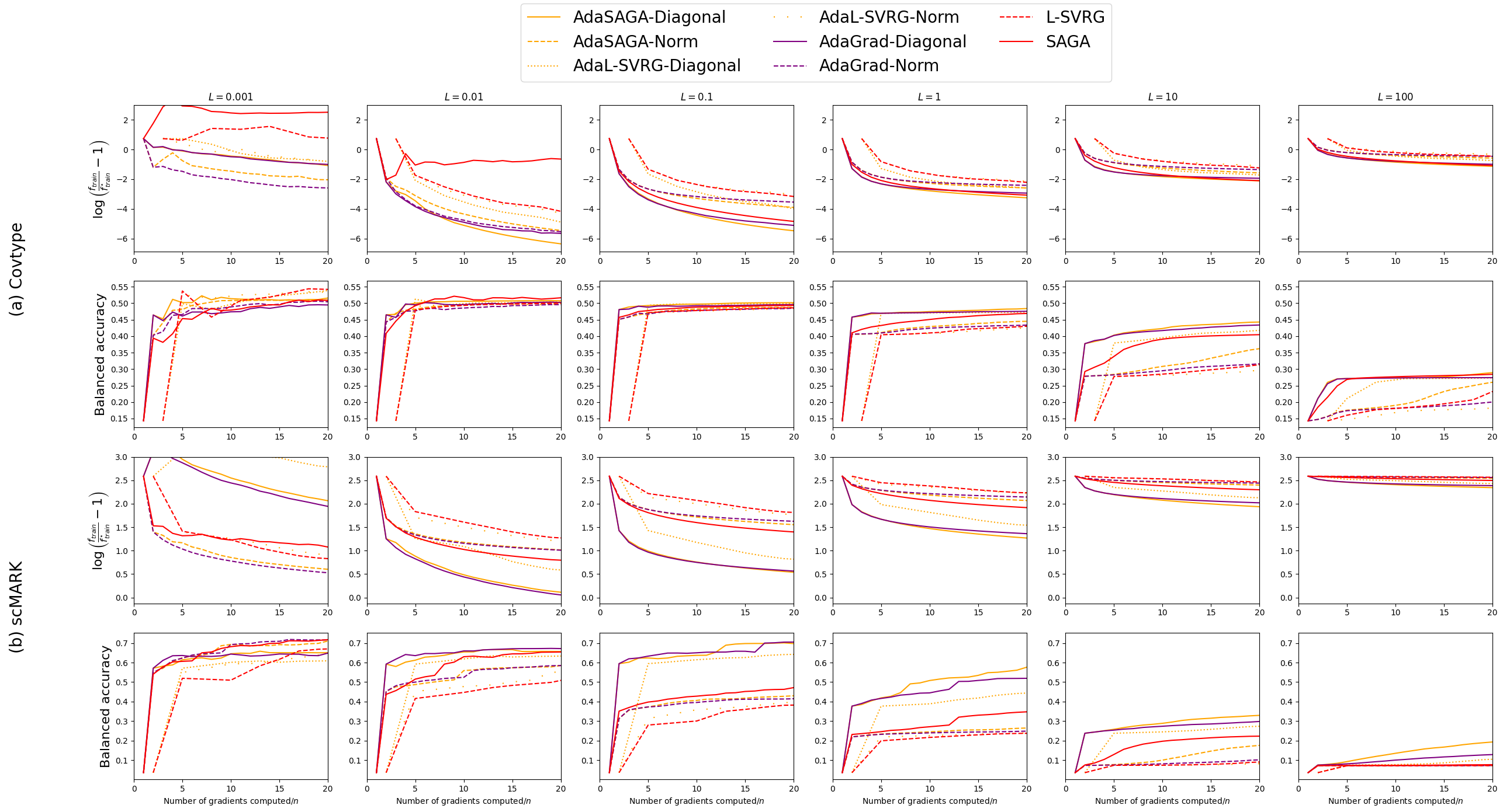
Figure 1: Comparison of AdaVR against SAGA, L-SVRG and AdaGrad.

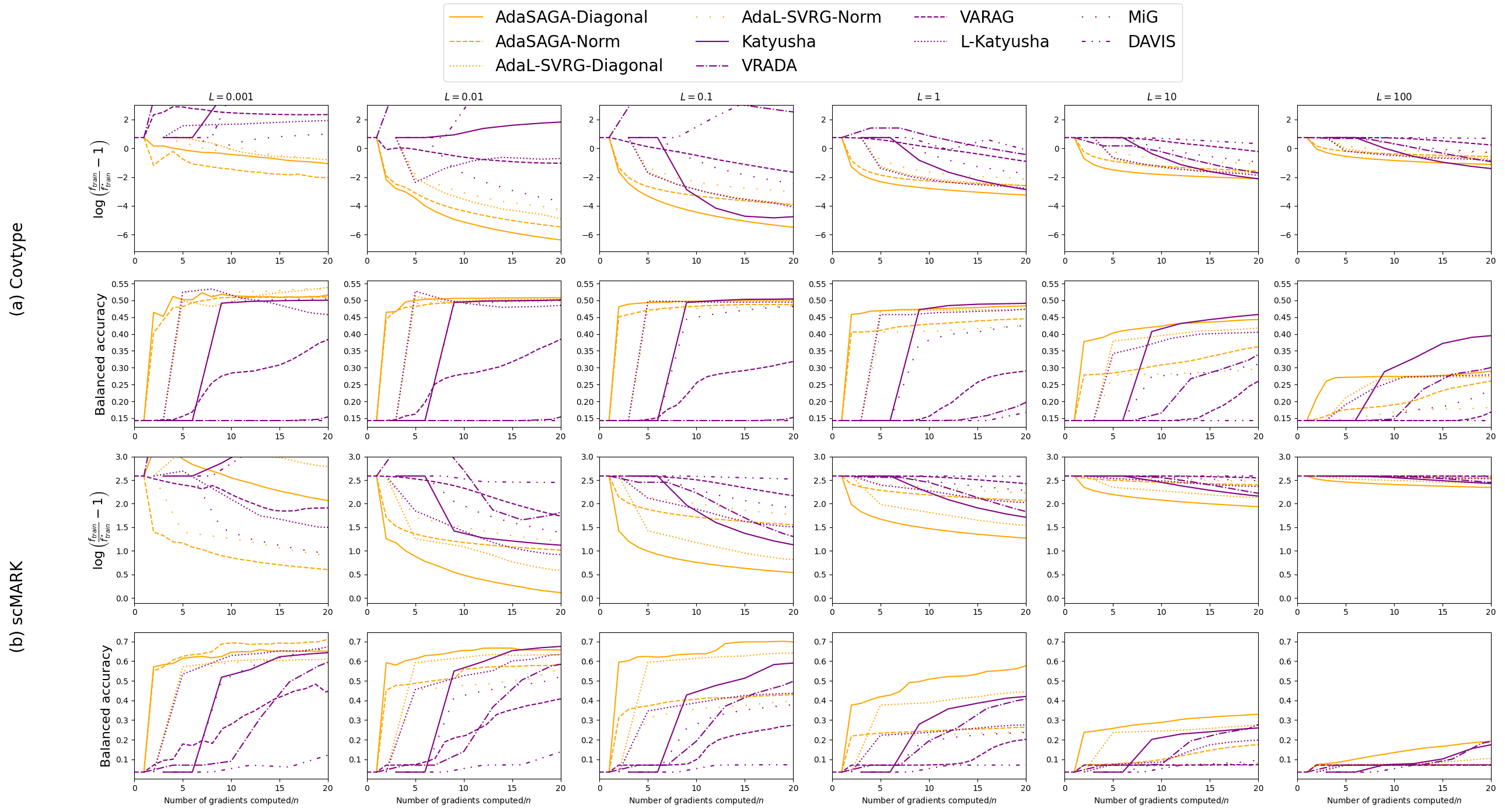
Figure 2: Comparison of AdaVR against accelerated algorithms with variance reduction.

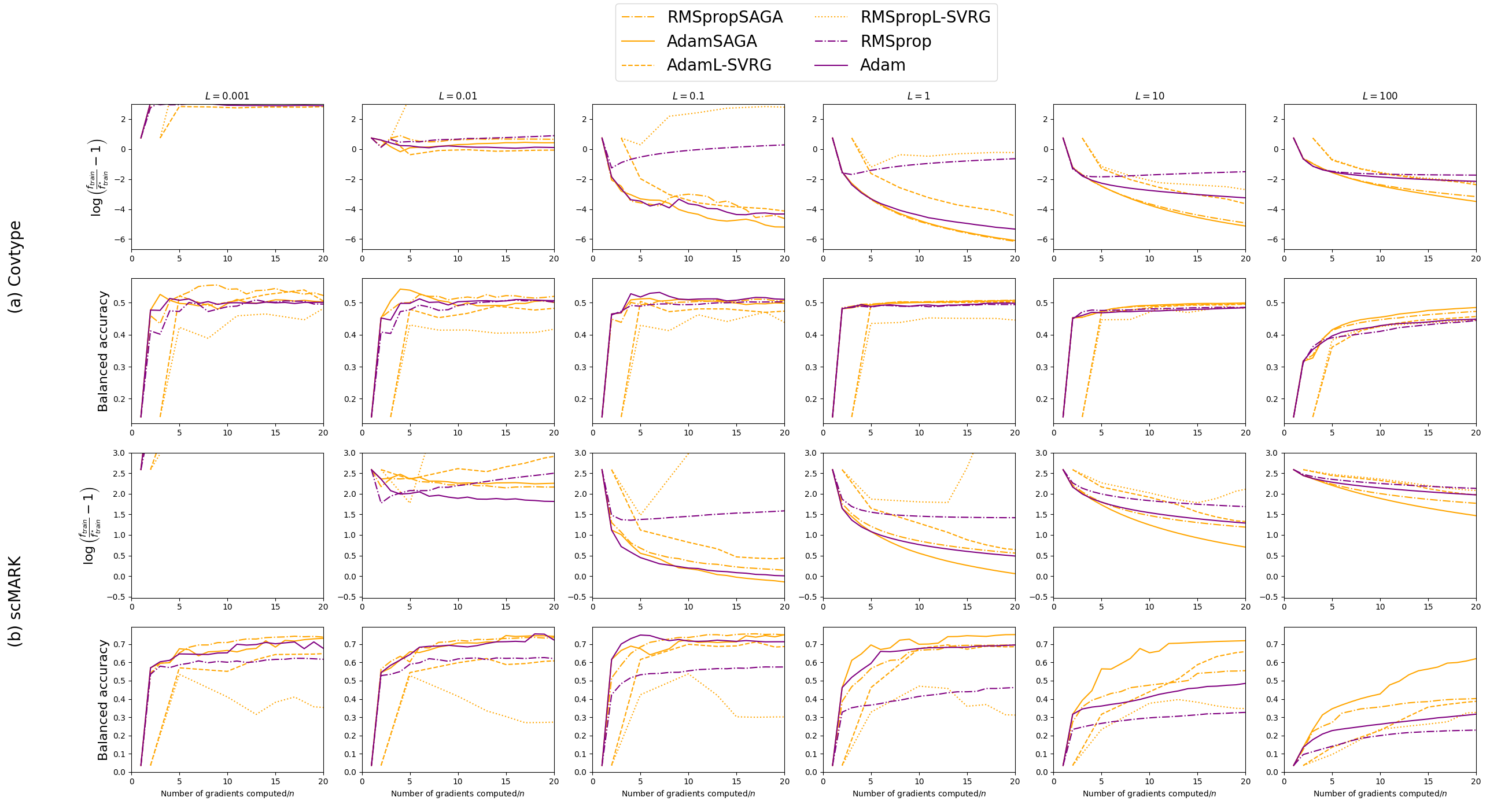
Figure 3: Comparison of Adam and RMSprop with and without variance reduction.

We define AdaVR in Section 3, a family of algorithms which allows for four different variants, by combining either AdaGrad-Norm or AdaGrad-Diagonal with either SAGA or L-SVRG type gradient estimators.

Theorem 3.2.

Let $T\geqslant 1,\eta>0,x^{(1)}\in\mathbb{R}^{d}$ and $\left(x^{(t)}\right)_{1\leqslant t\leqslant T}$ be a sequence of iterates defined by Section 3 with $p=1/n$, and where the AdaGrad variant (Norm or Diagonal) and the gradient estimator type (SAGA or L-SVRG) are chosen at the beginning and remain constant. Then, under Assumptions 2.1 and 2.2, it holds that:

$$\textstyle{\mathbb{E}\left[f(\overline{x}_{T})\right]-f\left(x^{\star}\right)\leqslant\frac{\alpha\left(\eta+\frac{D^{2}}{2\eta}\right)\sqrt{4Ln\Delta_{1}}+8L\alpha^{2}\left(\eta+\frac{D^{2}}{2\eta}\right)^{2}}{T}},$$

where $\overline{x}_{T}=\frac{1}{T}\sum_{t=1}^{T}x^{(t)}$, $\Delta_{1}=f\left(x^{(1)}\right)-f\left(x^{\star}\right)$ and $\alpha=1$ (resp. $\alpha=\sqrt{d}$) for the Norm variant (resp. the Diagonal variant).

The above convergence guarantee corresponds to a gradient complexity of $O(n+(L+\sqrt{nL})/T)$ which holds adaptively to the smoothness coefficient $L$.

4 Numerical experiments

We conduct numerical experiments to assess the good empirical performance of AdaVR over AdaGrad, SAGA, L-SVRG as well as state-of-the-art accelerated variance-reduced algorithms. We also consider as heuristics RMSprop and Adam combined with SAGA and L-SVRG type gradient estimators. We consider multivariate logistic regression with no regularization on the Covtype and scMARK datasets [Diaz-Mejia, 2021].

Experimental details and preprocessing

The Covtype dataset has $n=581012$ samples ($30\times 30$ meter cell) with 54 categorical features (cartographic variables). Each sample is labeled by its forest cover type, taking 7 different values. scMARK is a benchmark for scRNA data (single-cell Ribonucleic acid) with $n=19998$ samples (cells) and 14059 features (gene expression). Each sample is labeled by its cell type, taking 28 different values. We only keep the 300 features with largest variance. A min-max scaler is applied as preprocessing to both datasets as well as a train-test split procedure ($n_{\text{train}}\simeq 0.8n$, $n_{\text{test}}\simeq 0.2n$). We evaluate each algorithm based on two metrics: the objective function i.e. multivariate logistic regression loss computed on the train set and the balanced accuracy score i.e. a weighted average of the accuracy score computed on the test set.

For the covtype (resp. scMARK) dataset, we use a mini-batch size of $10$ (resp. $1$), and the dimension of the parameter space is $d=378=54\times 7$ (resp. $d=8400=28\times 300$). Experiments were run on a machine with 32 CPU cores and 64 GB of memory.

For most algorithms (including SAG, SAGA, (L-)SVRG, and accelerated variants), the hyperparameter $\eta$ must typically be chosen proportionnally to the inverse of $L$ to yield the best convergence guarantees, and larger values may lead to divergence. However, such a choice often leads to poor practical performances and a larger values of $\eta$ may result in faster convergence. Besides, the smoothness coefficient $L$ may be unknown. Other algorithms such as AdaGrad has guaranteed convergence for all values of its hyperparameter, but the performance still depends on its value. The most common approach is to tune $\eta$ via a ressource-heavy grid-search. We compare the performance of the algorithms for several values of their respective hyperparameters, each value corresponding to a guess of the value of the smoothness parameter $L$. Although there is no a priori relation between $L$ and the hyperparameter of adaptive algorithms based on AdaGrad, RMSprop and Adam, their hyperparameter is chosen on the same grid as the other algorithms, for ease of comparison.

AdaVR against SAGA, L-SVRG and AdaGrad

Following customary practice, we skip the projection step in AdaGrad and its variants. More attention will be put on the Diagonal versions of AdaGrad and AdaVR since they outperform the Norm versions in almost all cases. We compare AdaVR against SAGA, L-SVRG and AdaGrad in Figure 1. We observe that adding the SAGA variance reduction gradient estimator to AdaGrad-Diagonal gives a faster convergence of the objective function for $10$ out of $12$ plots (all except (b): $L=0.001,0.01$). The balanced accuracy is better or equivalent for AdaSAGA-Diagonal in every plot, and significantly better in $7$ out of $12$ plots ((a): $L=0.001,1,10,100$, (b): $L=1,10,100$). In (a), AdaVR-Diagonal gives similar balanced accuracy to SAGA but goes closer to the optimum and converges in more plots. In (b), the AdaVR-Diagonal is much more robust to the choice of the hyperparameter than SAGA or L-SVRG, giving good balanced accuracy for $4$ plots out of $6$ ($L=0.001,0.01,0.1,1$), and only $2$ for SAGA and L-SVRG ($L=0.001,0.01$). The perfomances of AdaVR-Diagonal in terms of objective function are much better than SAGA or L-SVRG, going closer to the optimum in more plots.

AdaVR against accelerated and variance-reduced algorithms

We compare AdaVR against state-of-the-art accelerated algorithms (MiG, Katyusha, L-Katyusha, VRADA, VARAG, DAVIS) in Figure 2. We observe that accelerated algorithms are sensitive to the choice of the hyperparameter and converge only when its value is small enough. By contrast, AdaVR is much more robust to the choice of the hyperparameter, converging in more plots.

RMSprop and Adam with variance-reduced gradient estimator

We here suggest the combination variance reduction with the RMSprop and Adam algorithms, which are variants of AdaGrad-Diagonal, that demonstrate much better practical performance.

AdaGrad accumulates the magnitute of the gradient estimators $g^{(t)}$ to adapt its stepsize, so that the coefficients of $G_{t}$ (resp. $A_{t}^{-1}$) can only increase (resp. decrease) which may slow optimization down. RMSprop [Ruder, 2017] remedies this by replacing the accumulation (meaning the regular sum) by a discounted sum, thereby allowing the $G_{t}$ quantity to decrease:

$$G_{t}=\gamma\operatorname{diag}\left(g^{(t)}g^{(t)\top}\right)+\left(1-\gamma\right)G_{t-1},\quad t\geqslant 1,$$ (1)

with $0<\gamma<1$. Adam [Kingma and Ba, 2015] also adds momentum:

$$\begin{array}[]{ll}&m^{(t)}=\beta_{1}m^{(t-1)}+\left(1-\beta_{1}\right)g^{(t)}\\ &G_{t}=\beta_{2}G_{t-1}+\left(1-\beta_{2}\right)\operatorname{diag}\left(g^{(t)}g^{(t)\top}\right),\\ &x^{(t+1)}=x^{(t)}-\eta G_{t}^{-\nicefrac{{1}}{{2}}}m^{(t)},\end{array}$$ (2)

with $0<\beta_{1},\beta_{2}<1$. Both algorithms demonstrate excellent performance and have given rise to many variants, even though their theoretical properties are less understood than AdaGrad. We suggest replacing $g^{(t)}$ by SAGA or L-SVRG-type gradient estimator in (1) and (2). Numerical experiments are plotted in Figure 3 (we set $\gamma=0.9$ for RMSprop and $\beta_{1}=0.9,\beta_{2}=0.999$ for Adam). Regarding the objective function, the effectiveness of the method clearly appears for RMSpropSAGA, AdamSAGA and AdamL-SVRG in $8$ plots out of $12$ ($L=0.1,1,10,100$), while RMSprop struggles to converge when combined with L-SVRG. The balanced accuracy is always greater or equal when adding the SAGA-type gradient estimator, giving significantly better results for $7$ plots out of $12$ ((a): $L=10,100$ and all plots of (b) except $L=0.01$) and is sometimes multiplied by $2$ (AdamSAGA in (b): $L=100$, RMSpropSAGA in (b): $L=10,100$).

5 Conclusion and perspectives

In the context of the minimization of a sum of $L$-smooth convex functions, we introduce AdaVR, combining AdaGrad and SAGA or L-SVRG-type gradient estimators. We demonstrate that AdaVR takes the best of both worlds, inheriting adaptiveness and low sensitivity to the hyperparameter from AdaGrad, and fast convergence rates from variance-reduced methods. We empirically show that Adam and RMSprop benefit from variance reduction even more.

A natural follow-up of this work would be to combine AdaGrad with acceleration techniques and loopless variance reduction to match the optimal gradient complexity. Another improvement would be to consider composite functions containing a possibly non-smooth regularization term. Besides, the study of the nonconvex and strongly convex cases are of interest. While not performed in practice, we rely on the projection step to obtain convergence guarantees, and an analysis of AdaVR without projection would be relevant. In addition, more general classes of variance reduced algorithms—e.g. JacSketch [Gower et al., 2021], Memorization Algorithms [Hofmann et al., 2015]; may be analyzed along with AdaGrad, allowing in particular to perform non-uniform sampling, the use of mini-batches, and variants of SAGA with low memory requirements. Finally, convergence guarantees for Adam and RMSprop combined with variance reduction is an interesting line of research.

Appendix A Proofs

See 3.1

Proof.

Let $1\leqslant t\leqslant T$ and consider $z\triangleq x^{(t)}-\eta A_{t}^{-1}g^{(t)}$ so that

$$z-x^{\star}=x^{(t)}-x^{\star}-\eta A_{t}^{-1}g^{(t)}.$$ (3)

Multiplying both sides by $A_{t}$ and using $A_{t}A_{t}^{-1}g^{(t)}=g^{(t)}$ (B.7), we get

$$A_{t}\left(z-x^{\star}\right)=A_{t}\left(x^{(t)}-x^{\star}\right)-\eta g^{(t)}.$$ (4)

Taking the scalar product of (3) and (4)

$$\left\langle z-x^{\star},A_{t}\left(z-x^{\star}\right)\right\rangle= \left\langle x^{(t)}-x^{\star},A_{t}\left(x^{(t)}-x^{\star}\right)\right\rangle-\eta\left\langle g^{(t)},x^{(t)}-x^{\star}\right\rangle$$

$$-\eta\left\langle A_{t}^{-1}g^{(t)},A_{t}\left(x^{(t)}-x^{\star}\right)\right\rangle+\eta^{2}\left\langle g^{(t)},A_{t}^{-1}g^{(t)}\right\rangle.$$

Using B.7 once again gives

$$\left\langle A_{t}^{-1}g^{(t)},A_{t}\left(x^{(t)}-x^{\star}\right)\right\rangle=\left\langle A_{t}A_{t}^{-1}g^{(t)},x^{(t)}-x^{\star}\right\rangle=\left\langle g^{(t)},x^{(t)}-x^{\star}\right\rangle$$

so that

$$\left\langle z-x^{\star},A_{t}\left(z-x^{\star}\right)\right\rangle=\left\langle x^{(t)}-x^{\star},A_{t}\left(x^{(t)}-x^{\star}\right)\right\rangle-2\eta\left\langle g^{(t)},x^{(t)}-x^{\star}\right\rangle+\eta^{2}\left\langle g^{(t)},A_{t}^{-1}g^{(t)}\right\rangle.$$

Rearranging the terms gives

$$\left\langle g^{(t)},x^{(t)}-x^{\star}\right\rangle =\frac{\eta}{2}\left\|g^{(t)}\right\|^{2}_{A_{t}^{-1}}+\frac{1}{2\eta}\left(\left\|x^{(t)}-x^{\star}\right\|_{A_{t}}^{2}-\left\|z-x^{\star}\right\|_{A_{t}}^{2}\right)$$

$$\leqslant\frac{\eta}{2}\left\|g^{(t)}\right\|^{2}_{A_{t}^{-1}}+\frac{1}{2\eta}\left(\left\|x^{(t)}-x^{\star}\right\|_{A_{t}}^{2}-\left\|x^{(t+1)}-x^{\star}\right\|_{A_{t}}^{2}\right).$$

We used $\left\|x^{(t+1)}-x^{\star}\right\|_{A_{t}}\leqslant\left\|z-x^{\star}\right\|_{A_{t}}$ since $x^{(t+1)}=\Pi_{X,A_{t}}\left(z\right)$. Summing the second term of the above right hand side gives

$$\sum_{t=1}^{T}\left(\left\|x^{(t)}-x^{\star}\right\|_{A_{t}}^{2}-\left\|x^{(t+1)}-x^{\star}\right\|_{A_{t}}^{2}\right)= \sum_{t=1}^{T}\left\|x^{(t)}-x^{\star}\right\|_{A_{t}}^{2}-\sum_{t=2}^{T+1}\left\|x^{(t)}-x^{\star}\right\|_{A_{t-1}}^{2}$$

$$= \sum_{t=1}^{T}\left(\left\|x^{(t)}-x^{\star}\right\|_{A_{t}}^{2}-\left\|x^{(t)}-x^{\star}\right\|_{A_{t-1}}^{2}\right)+\left\|x^{(1)}-x^{\star}\right\|_{A_{0}}^{2}$$

$$-\left\|x^{(T+1)}-x^{\star}\right\|_{A_{T}}^{2}$$

$$\leqslant \sum_{t=1}^{T}\left\|x^{(t)}-x^{\star}\right\|_{A_{t}-A_{t-1}}^{2},$$

where $A_{0}=0$ so that $\left\|x^{(1)}-x^{\star}\right\|^{2}_{A_{0}}=0$. Now, using B.8 and the first inequality of B.9 gives

$$\sum_{t=1}^{T}\left\langle g^{(t)},x^{(t)}-x^{\star}\right\rangle \leqslant\frac{\eta}{2}\sum_{t=1}^{T}\left\|g^{(t)}\right\|^{2}_{A_{t}^{-1}}+\frac{1}{2\eta}\left(\sum_{t=2}^{T}\left\|x^{(t)}-x^{\star}\right\|_{A_{t}-A_{t-1}}^{2}\right)$$

$$\leqslant\left(\eta+\frac{D^{2}}{2\eta}\right)\operatorname{Tr}(A_{T}),$$

Using the second inequality of B.9 ends the proof. ∎

Proposition A.1.

Let $T\geqslant 1$ and $\left(x^{(t)}\right)_{1\leqslant t\leqslant T}$ defined by Section 3. Then,

$$\mathbb{E}\left[\sum_{t=1}^{T}\mathbb{E}_{t}\left[\left\|g^{(t)}\right\|^{2}\right]\right]\leqslant\mathbb{E}\left[8L\sum_{t=1}^{T}\left(f\left(x^{(t)}\right)-f\left(x^{\star}\right)\right)\right]+4Ln\left(f\left(x^{(1)}\right)-f\left(x^{\star}\right)\right).$$

Proof.

Let 1 $\leqslant t\leqslant T$. We first deal with the case of SAGA-type gradient estimator. Using B.6 with $y^{(t)}_{i}=\tilde{x}^{(t)}_{i}\left(1\leqslant i\leqslant n\right)$ gives

$$\mathbb{E}_{t}\left[\left\|g^{(t)}\right\|^{2}\right]\leqslant 2\mathbb{E}_{t}\left[\left\|\nabla f_{i(t)}\left(x^{(t)}\right)-\nabla f_{i(t)}\left(x^{\star}\right)\right\|^{2}\right]+2\mathbb{E}_{t}\left[\left\|\nabla f_{i(t)}\left(\tilde{x}^{(t-1)}_{i(t)}\right)-\nabla f_{i(t)}\left(x^{\star}\right)\right\|^{2}\right].$$

Using B.3 for the first term and B.4 for the second gives:

$$\mathbb{E}_{t}\left[\left\|g^{(t)}\right\|^{2}\right]\leqslant 4L\left(f\left(x^{(t)}\right)-f\left(x^{\star}\right)\right)$$

$$+4L\left(f\left(x^{(t)}\right)-f\left(x^{\star}\right)+\sum_{i=1}^{n}D_{f_{i}}\left(\tilde{x}^{(t-1)}_{i},x^{\star}\right)-\mathbb{E}_{t}\left[\sum_{i=1}^{n}D_{f_{i}}\left(\tilde{x}^{(t)}_{i},x^{\star}\right)\right]\right)$$

$$= 8L\left(f\left(x^{(t)}\right)-f\left(x^{\star}\right)\right)+4L\left(\sum_{i=1}^{n}D_{f_{i}}\left(\tilde{x}^{(t-1)}_{i},x^{\star}\right)-\mathbb{E}_{t}\left[\sum_{i=1}^{n}D_{f_{i}}\left(\tilde{x}^{(t)}_{i},x^{\star}\right)\right]\right).$$

Summing in $t$ and taking the expectation gives

$$\mathbb{E}\left[\sum_{t=1}^{T}\mathbb{E}_{t}\left[\left\|g^{(t)}\right\|^{2}\right]\right] \leqslant\mathbb{E}\left[8L\sum_{t=1}^{T}\left(f\left(x^{(t)}\right)-f\left(x^{\star}\right)\right)+4L\sum_{t=1}^{T}\left(\sum_{i=1}^{n}D_{f_{i}}\left(\tilde{x}^{(t-1)}_{i},x^{\star}\right)-\mathbb{E}_{t}\left[\sum_{i=1}^{n}D_{f_{i}}\left(\tilde{x}^{(t)}_{i},x^{\star}\right)\right]\right)\right]$$

$$=\mathbb{E}\left[8L\sum_{t=1}^{T}\left(f\left(x^{(t)}\right)-f\left(x^{\star}\right)\right)+4L\sum_{t=1}^{T}\left(\sum_{i=1}^{n}D_{f_{i}}\left(\tilde{x}^{(t-1)}_{i},x^{\star}\right)-\sum_{i=1}^{n}D_{f_{i}}\left(\tilde{x}^{(t)}_{i},x^{\star}\right)\right)\right]$$

$$\leqslant\mathbb{E}\left[8L\sum_{t=1}^{T}\left(f\left(x^{(t)}\right)-f\left(x^{\star}\right)\right)\right]+4L\underbrace{\sum_{i=1}^{n}D_{f_{i}}\left(\tilde{x}_{i}^{(0)},x^{\star}\right)}_{=n\left(f\left(x^{(1)}\right)-f\left(x^{\star}\right)\right)},$$ (5)

where we used the tower property at the second line, recognized a telescopic sum at the last line and removed its last term since nonpositive, hence the result.

We turn to the case of L-SVRG type gradient estimator. Using B.6 with $y^{(t)}_{i}=\tilde{x}^{(t)}\left(1\leqslant i\leqslant n\right)$ gives

$$\mathbb{E}_{t}\left[\left\|g^{(t)}\right\|^{2}\right]\leqslant 2\mathbb{E}_{t}\left[\left\|\nabla f_{i(t)}\left(x^{(t)}\right)-\nabla f_{i(t)}\left(x^{\star}\right)\right\|^{2}\right]+2\mathbb{E}_{t}\left[\left\|\nabla f_{i(t)}\left(\tilde{x}^{(t-1)}\right)-\nabla f_{i(t)}\left(x^{\star}\right)\right\|^{2}\right].$$

Using B.3 on the first term and B.5 on the second gives:

$$\mathbb{E}_{t}\left[\left\|g^{(t)}\right\|^{2}\right]\leqslant 4L\left(f\left(x^{(t)}\right)-f\left(x^{\star}\right)\right)$$

$$+4L\left(f\left(x^{(t)}\right)-f\left(x^{\star}\right)+\sum_{i=1}^{n}D_{f_{i}}\left(\tilde{x}^{(t-1)},x^{\star}\right)-\mathbb{E}_{t}\left[\sum_{i=1}^{n}D_{f_{i}}\left(\tilde{x}^{(t)},x^{\star}\right)\right]\right)$$

$$= 8L\left(f\left(x^{(t)}\right)-f\left(x^{\star}\right)\right)+4L\left(\sum_{i=1}^{n}D_{f_{i}}\left(\tilde{x}^{(t-1)},x^{\star}\right)-\mathbb{E}_{t}\left[\sum_{i=1}^{n}D_{f_{i}}\left(\tilde{x}^{(t)},x^{\star}\right)\right]\right).$$

Summing in $t$ and taking the expectation gives

$$\mathbb{E}\left[\sum_{t=1}^{T}\mathbb{E}_{t}\left[\left\|g^{(t)}\right\|^{2}\right]\right] \leqslant\mathbb{E}\left[8L\sum_{t=1}^{T}\left(f\left(x^{(t)}\right)-f\left(x^{\star}\right)\right)+4L\sum_{t=1}^{T}\left(\sum_{i=1}^{n}D_{f_{i}}\left(\tilde{x}^{(t-1)},x^{\star}\right)-\mathbb{E}_{t}\left[\sum_{i=1}^{n}D_{f_{i}}\left(\tilde{x}^{(t)},x^{\star}\right)\right]\right)\right]$$

$$=\mathbb{E}\left[8L\sum_{t=1}^{T}\left(f\left(x^{(t)}\right)-f\left(x^{\star}\right)\right)+4L\sum_{t=1}^{T}\left(\sum_{i=1}^{n}D_{f_{i}}\left(\tilde{x}^{(t-1)},x^{\star}\right)-\sum_{i=1}^{n}D_{f_{i}}\left(\tilde{x}^{(t)},x^{\star}\right)\right)\right]$$

$$\leqslant\mathbb{E}\left[8L\sum_{t=1}^{T}\left(f\left(x^{(t)}\right)-f\left(x^{\star}\right)\right)\right]+4L\underbrace{\sum_{i=1}^{n}D_{f_{i}}\left(\tilde{x}^{(0)},x^{\star}\right)}_{=n\left(f\left(x^{(1)}\right)-f\left(x^{\star}\right)\right)},$$ (6)

hence the result.∎

See 3.2

Proof.

We set $\Delta_{T}\triangleq\sum_{t=1}^{T}\mathbb{E}\left[f\left(x^{(t)}\right)-f\left(x^{\star}\right)\right]$ and $\gamma\triangleq\alpha\left(\eta+\frac{D^{2}}{\eta}\right)$ (where $\alpha=1$ (resp. $\alpha=\sqrt{d}$) in the case of the Norm version (resp. the Diagonal version)). Using the convexity of $f$, Lemmas 3.1 and B.10, and Proposition A.1,

$$\Delta_{T} \leqslant\mathbb{E}\left[\sum_{t=1}^{T}\left<\nabla f(x^{(t)}),x^{(t)}-x^{*}\right>\right]=\mathbb{E}\left[\sum_{t=1}^{T}\mathbb{E}_{t}\left[\left<g^{(t)},x^{(t)}-x^{*}\right>\right]\right]$$

$$\leqslant\gamma\mathbb{E}\left[\sqrt{\sum_{t=1}^{T}\left\|g^{(t)}\right\|^{2}}\right]\leqslant\gamma\sqrt{\mathbb{E}\left[\sum_{t=1}^{T}\left\|g^{(t)}\right\|^{2}\right]}$$

$$\leqslant\gamma\sqrt{\mathbb{E}\left[8L\sum_{t=1}^{T}\left(f(x^{(t)})-f(x^{*})\right)\right]+4Ln\left(f(x^{(1)})-f(x^{*})\right)}$$

$$=\gamma\sqrt{L\left(8\Delta_{T}+4n(f(x^{(1)})-f(x^{*}))\right)}.$$

Using B.11 gives

$$\Delta_{T}\leqslant 8L\gamma^{2}+\gamma\sqrt{4L\left(f\left(x^{(1)}\right)-f\left(x^{\star}\right)\right)}.$$

By convexity, $\Delta_{T}\geqslant T\mathbb{E}\left[f(\overline{x}_{T})-f(x^{*})\right]$ and the result follows. ∎

Appendix B Helper Lemmas

The Bregman divergence associated with a differentiable function $g:\mathbb{R}^{d}\to\mathbb{R}$ is defined as

$$D_{g}(y,x)=g(y)-g(x)-\left<\nabla g(x),y-x\right>,\qquad x,y\in\mathbb{R}^{d}.$$

When $g$ is convex, the Bregman divergence is always nonnegative.

Lemma B.1 ([Nesterov, 2004] Theorem 2.1.5).

If $g$ is an $L$-smooth convex function

$$\frac{1}{2L}\left\|\nabla g(x)-\nabla g(y)\right\|^{2}\leqslant D_{g}(y,x),\quad x,y\in\mathbb{R}^{d}.$$

Corollary B.2.

Under Assumptions 2.1 and 2.2,

$$\left\|\nabla f(x)\right\|\leqslant 2L\left(f(x)-f\left(x^{\star}\right)\right),\quad x\in\mathbb{R}^{d}.$$

Proof.

Let $x\in\mathbb{R}^{d}$. Using B.1 gives

$$\left\|\nabla f(x)\right\|=\left\|\nabla f(x)-\nabla f\left(x^{\star}\right)\right\|\leqslant 2LD_{f}(x,x^{\star})=2L\left(f(x)-f\left(x^{\star}\right)\right).$$

∎

Corollary B.3.

For Section 3 and under Assumptions 2.1 and 2.2, for all $1\leqslant t\leqslant T$, we have

$$\mathbb{E}_{t}\left[\left\|\nabla f_{i(t)}\left(x^{(t)}\right)-\nabla f_{i(t)}\left(x^{\star}\right)\right\|^{2}\right]\leqslant 2L\left(f\left(x^{(t)}\right)-f\left(x^{\star}\right)\right).$$

Proof.

$$\mathbb{E}_{t}\left[\left\|\nabla f_{i(t)}\left(x^{(t)}\right)-\nabla f_{i(t)}\left(x^{\star}\right)\right\|^{2}\right] =\frac{2L}{2L}\frac{1}{n}\sum_{i=1}^{n}\left\|\nabla f_{i}\left(x^{(t)}\right)-\nabla f_{i}\left(x^{\star}\right)\right\|^{2}$$

$$\leqslant\frac{2L}{n}\sum_{i=1}^{n}D_{f_{i}}(x^{(t)},x^{\star})$$ (B.1)

$$=\frac{2L}{n}\sum_{i=1}^{n}\left(f_{i}\left(x^{(t)}\right)-f_{i}\left(x^{\star}\right)-\left\langle\nabla f_{i}\left(x^{\star}\right),x^{(t)}-x^{\star}\right\rangle\right)$$

$$=2L\left(f\left(x^{(t)}\right)-f\left(x^{\star}\right)-0\right),$$

where in the last line we used the finite-sum structure of $f$ and $\nabla f\left(x^{\star}\right)=0$. ∎

Lemma B.4.

For Section 3 with SAGA and under Assumptions 2.1 and 2.2, for all $1\leqslant t\leqslant T$, we have

$$\frac{1}{2L}\mathbb{E}_{t}\left[\left\|\nabla f_{i(t)}\left(\tilde{x}^{(t-1)}_{i(t)}\right)-\nabla f_{i(t)}\left(x^{\star}\right)\right\|^{2}\right]\leqslant f\left(x^{(t)}\right)-f\left(x^{\star}\right)+\sum_{i=1}^{n}D_{f_{i}}\left(\tilde{x}_{i}^{(t-1)},x^{\star}\right)-\mathbb{E}_{t}\left[\sum_{i=1}^{n}D_{f_{i}}\left(\tilde{x}_{i}^{(t)},x^{\star}\right)\right].$$

Proof.

First, from B.1

$$\frac{1}{2L}\mathbb{E}_{t}\left[\left\|\nabla f_{i(t)}\left(\tilde{x}^{(t-1)}_{i(t)}\right)-\nabla f_{i(t)}\left(x^{\star}\right)\right\|^{2}\right]\leqslant\mathbb{E}_{t}\left[D_{f_{i(t)}}\left(\tilde{x}_{i(t)}^{(t-1)},x^{\star}\right)\right]=\frac{1}{n}\sum_{i=1}^{n}D_{f_{i}}\left(\tilde{x}_{i}^{(t-1)},x^{\star}\right).$$

By definition, for all $1\leqslant i\leqslant n$, $\tilde{x}^{(t)}_{i}|x^{(t)}=\left\{\begin{array}[]{ll}x^{(t)}&\mbox{with probability }1/n\\ \tilde{x}^{(t-1)}_{i}&\mbox{with probability }1-1/n\end{array}\right.$. Therefore,

$$\mathbb{E}_{t}\left[\sum_{i=1}^{n}D_{f_{i}}\left(\tilde{x}_{i}^{(t)},x^{\star}\right)\right]=\frac{1}{n}\sum_{i=1}^{n}D_{f_{i}}(x^{(t)},x^{\star})+\frac{n-1}{n}\sum_{i=1}^{n}D_{f_{i}}\left(\tilde{x}_{i}^{(t-1)},x^{\star}\right).$$

Reorganizing the terms and using

$$\frac{1}{n}\sum_{i=1}^{n}D_{f_{i}}(x^{(t)},x^{\star})=\frac{1}{n}\sum_{i=1}^{n}\left(f_{i}\left(x^{(t)}\right)-f_{i}\left(x^{\star}\right)-\left\langle\nabla f_{i}\left(x^{\star}\right),x^{(t)}-x^{\star}\right\rangle\right)=f\left(x^{(t)}\right)-f\left(x^{\star}\right)-0$$

gives

$$\frac{1}{n}\sum_{i=1}^{n}D_{f_{i}}\left(\tilde{x}_{i}^{(t-1)},x^{\star}\right)=f\left(x^{(t)}\right)-f\left(x^{\star}\right)+\sum_{i=1}^{n}D_{f_{i}}\left(\tilde{x}_{i}^{(t-1)},x^{\star}\right)-\mathbb{E}_{t}\left[\sum_{i=1}^{n}D_{f_{i}}\left(\tilde{x}_{i}^{(t)},x^{\star}\right)\right],$$

hence the result. ∎

Lemma B.5.

For Section 3 with L-SVRG and under Assumptions 2.1 and 2.2, for all $1\leqslant t\leqslant T$, we have

$$\frac{1}{2L}\mathbb{E}_{t}\left[\left\|\nabla f_{i(t)}\left(\tilde{x}^{(t-1)}\right)-\nabla f_{i(t)}\left(x^{\star}\right)\right\|^{2}\right]\leqslant f\left(x^{(t)}\right)-f\left(x^{\star}\right)+\sum_{i=1}^{n}D_{f_{i}}\left(\tilde{x}^{(t-1)},x^{\star}\right)-\mathbb{E}_{t}\left[\sum_{i=1}^{n}D_{f_{i}}\left(\tilde{x}^{(t)},x^{\star}\right)\right].$$

Proof.

First, from B.1,

$$\frac{1}{2L}\mathbb{E}_{t}\left[\left\|\nabla f_{i(t)}\left(\tilde{x}^{(t-1)}\right)-\nabla f_{i(t)}\left(x^{\star}\right)\right\|^{2}\right]\leqslant\mathbb{E}_{t}\left[D_{f_{i(t)}}\left(\tilde{x}^{(t-1)},x^{\star}\right)\right]=\frac{1}{n}\sum_{i=1}^{n}D_{f_{i}}\left(\tilde{x}^{(t-1)},x^{\star}\right).$$

By definintion, $\tilde{x}^{(t)}|x^{(t)}=\left\{\begin{array}[]{ll}x^{(t)}&\mbox{with probability }1/n\\ \tilde{x}^{(t-1)}&\mbox{with probability }1-1/n\end{array}\right.,$ therefore,

$$\mathbb{E}_{t}\left[\sum_{i=1}^{n}D_{f_{i}}\left(\tilde{x}^{(t)},x^{\star}\right)\right]=\frac{1}{n}\sum_{i=1}^{n}D_{f_{i}}(x^{(t)},x^{\star})+\frac{n-1}{n}\sum_{i=1}^{n}D_{f_{i}}\left(\tilde{x}^{(t-1)},x^{\star}\right).$$

Reorganizing the terms and using

$$\frac{1}{n}\sum_{i=1}^{n}D_{f_{i}}(x^{(t)},x^{\star})=\frac{1}{n}\sum_{i=1}^{n}\left(f_{i}\left(x^{(t)}\right)-f_{i}\left(x^{\star}\right)-\left\langle\nabla f_{i}\left(x^{\star}\right),x^{(t)}-x^{\star}\right\rangle\right)=f\left(x^{(t)}\right)-f\left(x^{\star}\right)-0$$

gives

$$\frac{1}{n}\sum_{i=1}^{n}D_{f_{i}}\left(\tilde{x}^{(t-1)},x^{\star}\right)=f\left(x^{(t)}\right)-f\left(x^{\star}\right)+\sum_{i=1}^{n}D_{f_{i}}\left(\tilde{x}^{(t-1)},x^{\star}\right)-\mathbb{E}_{t}\left[\sum_{i=1}^{n}D_{f_{i}}\left(\tilde{x}^{(t)},x^{\star}\right)\right].$$

∎

Lemma B.6 ([Defazio, 2015] Lemma 4.5).

Under Assumptions 2.1 and 2.2. Let $t\geqslant 1$ and let $g^{(t)}$ be defined as

$$g^{(t)}=\nabla f_{i(t)}\left(x^{(t)}\right)-\nabla f_{i(t)}\left(y^{(t-1)}_{i(t)}\right)+\frac{1}{n}\sum_{i=1}^{n}\nabla f_{i}(y^{(t-1)}),$$

where $y^{(t-1)}_{i}\in\mathbb{R}^{d}\left(1\leqslant i\leqslant n\right)$ and $i(t)|x^{(t)}\sim\text{Unif}\{1,\dots,n\}$. We have,

$$\mathbb{E}_{t}\left[\left\|g^{(t)}\right\|^{2}\right]\leqslant 2\mathbb{E}_{t}\left[\left\|\nabla f_{i(t)}\left(x^{(t)}\right)-\nabla f_{i(t)}\left(x^{\star}\right)\right\|^{2}\right]+2\mathbb{E}_{t}\left[\left\|\nabla f_{i(t)}\left(y^{(t-1)}_{i(t)}\right)-\nabla f_{i(t)}\left(x^{\star}\right)\right\|^{2}\right].$$

Proof.

We give the proof for completeness. Using the definition of $g^{(t)}$,

$$\mathbb{E}_{t}\left[\left\|g^{(t)}\right\|^{2}\right] =\mathbb{E}_{t}\bigg{[}\bigg{\|}\nabla f_{i(t)}\left(x^{(t)}\right)-\nabla f_{i(t)}\left(y^{(t-1)}_{i(t)}\right)+\frac{1}{n}\sum_{i=1}^{n}\nabla f_{i}\left(y^{(t-1)}_{i}\right)\bigg{\|}\bigg{]}$$

$$=\mathbb{E}_{t}\bigg{[}\bigg{\|}\nabla f_{i(t)}\left(x^{(t)}\right)-\nabla f_{i(t)}\left(x^{\star}\right)-\bigg{(}\nabla f_{i(t)}\left(y^{(t-1)}_{i(t)}\right)-\nabla f_{i(t)}\left(x^{\star}\right)-\frac{1}{n}\displaystyle\sum_{i=1}^{n}\nabla f_{i}\left(y^{(t-1)}_{i}\right)\bigg{)}\bigg{\|}^{2}\bigg{]}$$

$$\leqslant 2\mathbb{E}_{t}\left[\left\|\nabla f_{i(t)}\left(x^{(t)}\right)-\nabla f_{i(t)}\left(x^{\star}\right)\right\|^{2}\right]$$

$$+2\mathbb{E}_{t}\Bigg{[}\bigg{\|}\underbrace{\nabla f_{i(t)}\left(y^{(t-1)}_{i(t)}\right)-\nabla f_{i(t)}\left(x^{\star}\right)}_{\triangleq X}-\bigg{[}\underbrace{\frac{1}{n}\sum_{i=1}^{n}\nabla f_{i}\left(y^{(t-1)}_{i}\right)-\overbrace{\nabla f\left(x^{\star}\right)}^{=0}}_{=\mathbb{E}_{t}\left[X\right]}\bigg{]}\bigg{\|}^{2}\Bigg{]}$$

$$\leqslant 2\mathbb{E}_{t}\left[\left\|\nabla f_{i(t)}\left(x^{(t)}\right)-\nabla f_{i(t)}\left(x^{\star}\right)\right\|^{2}\right]+2\mathbb{E}_{t}\left[\left\|\nabla f_{i(t)}\left(y^{(t-1)}_{i(t)}\right)-\nabla f_{i(t)}\left(x^{\star}\right)\right\|^{2}\right]$$

where we used basic inequalities $\left\|a+b\right\|^{2}\leqslant 2\left\|a\right\|^{2}+2\left\|b\right\|^{2}$ and $\mathbb{E}_{t}\left[\left\|X-\mathbb{E}_{t}\left[X\right]\right\|^{2}\right]\leqslant\mathbb{E}_{t}\left[\left\|X\right\|^{2}\right]$. ∎

Lemma B.7.

Let $\left(g^{(t)}\right)_{t\geqslant 1}$ be a sequence in $\mathbb{R}^{d}$. For $t\geqslant 1$, and let $A_{t}$ be defined as either

$$A_{t}=\sqrt{\sum_{s=1}^{t}\left\|g^{(s)}\right\|^{2}}\in\mathbb{R}\qquad\text{or}\qquad A_{t}=\sqrt{\sum_{s=1}^{t}\operatorname{diag}\left(g^{(s)}g^{(s)\top}\right)}\in\mathbb{R}^{d\times d},$$

where the square-root is to be understood component-wise. Then, $A_{t}A_{t}^{-1}g^{(t)}=g^{(t)}$, where $A_{t}^{-1}$ denotes the Moore–Penrose pseudo-inverse of $A_{t}$.

Proof.

Let $t\geqslant 1$. For the scalar case, if $g^{(t)}=0$ the identity holds. If $g^{(t)}\neq 0$, then $A_{t}>0$ so that $A_{t}A_{t}^{-1}=1$ and the identity holds.

For the diagonal case, let $1\leqslant k\leqslant d$. We denote $B_{kk}$ the $k^{\text{th}}$ diagonal term of a matrix $B\in\mathbb{R}^{d\times d}$. By definition of the Moore–Penrose pseudo-inverse, since $A_{t}$ is diagonal,

$$\left(A_{t}^{-1}\right)_{kk}=\begin{cases}\left(A_{t,kk}\right)^{-1}&\text{ if }A_{t,kk}>0\\ 0&\text{if }A_{t,kk}=0\end{cases}.$$

Because $A_{t}$ is diagonal,

$$\left(A_{t}A_{t}^{-1}g^{(t)}\right)_{k}=\left(A_{t}^{-1}\right)_{kk}A_{t,kk}g^{(t)}_{k}.$$

If $g^{(t)}_{k}=0$, then $\left(A_{t}^{-1}\right)_{k}A_{t,kk}g^{(t)}_{k}=0.$
If $g^{(t)}_{k}>0$, using the definition of $A_{t}$ gives $A_{t,kk}>0$ so that

$$\left(A_{t}^{-1}\right)_{kk}A_{t,kk}=1$$

and the identity is satisfied.

∎

The following lemma is adapted from Duchi et al. [2011, Theorem 7].

Lemma B.8.

Let $T\geqslant 1$ and $x\in X$. Then, for both AdaGrad-Norm and AdaGrad-Diagonal as defined in (AdaGrad), it holds that

$$\sum_{t=1}^{T}\left\|x^{(t)}-x\right\|^{2}_{A_{t}-A_{t-1}}\leqslant D^{2}\operatorname{Tr}(A_{T}).$$

Proof.

Remember that $A_{0}=0$ by convention. For $1\leqslant t\leqslant T$, it holds that $A_{t}-A_{t-1}\succeq 0$ by construction, so that

$$\sum_{t=1}^{T}\left\|x^{(t)}-x\right\|^{2}_{A_{t}-A_{t-1}} \leqslant\sum_{t=1}^{T}\left\|x^{(t)}-x\right\|^{2}\lambda_{\text{max}}\left(A_{t}-A_{t-1}\right)$$

$$\leqslant\sum_{t=1}^{T}\left\|x^{(t)}-x\right\|^{2}\operatorname{Tr}\left(A_{t}-A_{t-1}\right)$$

$$\leqslant\sum_{t=1}^{T}D^{2}\operatorname{Tr}\left(A_{t}-A_{t-1}\right)$$

$$=D^{2}\operatorname{Tr}(A_{T}).$$

∎

The following lemma is adapted from Duchi et al. [2011, Lemma 10].

Lemma B.9.

Let $T\geqslant 1$. For both AdaGrad-Norm and AdaGrad-Diagonal as defined in (AdaGrad):

$$\sum_{t=1}^{T}\left\|g^{(t)}\right\|^{2}_{A_{t}^{-1}}\leqslant 2\operatorname{Tr}(A_{T}).$$

Moreover,

$$\operatorname{Tr}(A_{T})\leqslant\alpha\sqrt{\sum_{t=1}^{T}\left\|g^{(t)}\right\|^{2}}$$

where $\alpha=1$ (resp. $\alpha=\sqrt{d}$) for AdaGrad-Norm (resp. AdaGrad-Diagonal).

Proof.

We proceed by induction. For $T=1$, for the scalar version we get

$$g^{(1)\top}A_{1}^{-1}g^{(1)}=A_{1}^{-1}\left\|g^{(1)}\right\|^{2}=A_{1}^{-1}A_{1}^{2}=A_{1}A_{1}^{-1}A_{1}=A_{1},$$

where the last equality follows from the definition of the Moore–Penrose inverse. For the diagonal version, we similarly have

$$g^{(1)^{\top}}A_{1}^{-1}g^{(1)} =\operatorname{Tr}\left(A_{1}^{-1}g^{(1)}g^{(1)^{\top}}\right)=\operatorname{Tr}\left(A_{1}^{-1}\operatorname{diag}\left(g^{(1)}g^{(1)^{\top}}\right)\right)$$

$$=\operatorname{Tr}\left(A_{1}^{-1}A_{1}^{2}\right)=\operatorname{Tr}\left(A_{1}A_{1}^{-1}A_{1}\right)=\operatorname{Tr}\left(A_{1}\right),$$

where we used the fact that if $A$ is diagonal and $B$ is arbitrary, then $\operatorname{Tr}(AB)=\operatorname{Tr}(A\operatorname{diag}(B))$. This proves the result for $T=1$. Let $T^{\prime}\geqslant 1$ and suppose it true for $T=T^{\prime}-1$. For both variants (seeing $A_{t}$ as a matrix of size 1 in the case of the scalar variant), we have

$$\sum_{t=1}^{T^{\prime}}g^{(t)\top}A_{t}^{-1}g^{(t)} =\sum_{t=1}^{T^{\prime}-1}g^{(t)\top}A_{t}^{-1}g^{(t)}+g^{(T^{\prime})\top}A_{T^{\prime}}^{-1}g^{(T^{\prime})}$$

$$\leqslant 2\operatorname{Tr}\left(A_{T^{\prime}-1}\right)+g^{(T^{\prime})\top}A_{T^{\prime}}^{-1}g^{(T^{\prime})}$$

$$=2\operatorname{Tr}\left(\left(A_{T^{\prime}}^{2}-g^{(T^{\prime})}g^{(T^{\prime})\top}\right)^{\nicefrac{{1}}{{2}}}\right)+\operatorname{Tr}\left(A_{T^{\prime}}^{-1}g^{(T^{\prime})}g^{(T^{\prime})\top}\right)$$

$$\leqslant 2\operatorname{Tr}(A_{T^{\prime}})$$

where we used the recurrence hypothesis at the second line and at the last line we used [Duchi et al., 2011, Lemma 8]:

$$X\succeq Y\succeq 0\implies 2\operatorname{Tr}\left(\left(X-Y\right)^{1/2}\right)+\operatorname{Tr}\left(X^{-1/2}Y\right)\leqslant 2\operatorname{Tr}\left(X^{1/2}\right),$$

finishing the induction step. For the bound on the trace, for the norm version we have

$$\operatorname{Tr}(A_{T})=G_{T}^{\nicefrac{{1}}{{2}}}=\sqrt{\sum_{t=1}^{T}\left\|g^{(t)}\right\|^{2}}$$

For the diagonal version we use Jensen’s inequality to get

$$\operatorname{Tr}(A_{T}) =\operatorname{Tr}\left(G_{T}^{\nicefrac{{1}}{{2}}}\right)=\sum_{j=1}^{d}\sqrt{\lambda_{j}\left(G_{T}\right)}$$

$$=d\sum_{j=1}^{d}\frac{1}{d}\sqrt{\lambda_{j}\left(G_{T}\right)}\leqslant d\sqrt{\sum_{j=1}^{d}\frac{1}{d}\lambda_{j}\left(G_{T}\right)}$$

$$=\sqrt{d\operatorname{Tr}\left(G_{T}\right)}$$

where $\lambda_{j}(G_{T})$ denotes the $j^{\text{th}}$ eigenvalue of $G_{T}$. Now,

$$\operatorname{Tr}\left(G_{T}\right)=\operatorname{Tr}\left(\sum_{t=1}^{T}\operatorname{diag}\left(g^{(t)\top}g^{(t)}\right)\right)=\sum_{t=1}^{T}\left\|g^{(t)}\right\|^{2},$$

ending the proof. ∎

Lemma B.10.

Let $1\leqslant t\leqslant T$, and $g^{(t)}$ be defined by Section 3. We have

$$\mathbb{E}_{t}\left[g^{(t)}\right]=\nabla f(x^{(t)}).$$

Proof.

In the case of SAGA-type gradient estimators,

$$\mathbb{E}_{t}\left[g^{(t)}\right] =\mathbb{E}_{t}\left[\nabla f_{i(t)}\left(x^{(t)}\right)-\nabla f_{i(t)}\left(\tilde{x}^{(t-1)}_{i(t)}\right)+\frac{1}{n}\sum_{i=1}^{n}\nabla f_{i}\left(\tilde{x}^{(t-1)}_{i}\right)\right]$$

$$=\frac{1}{n}\sum_{i=1}^{n}\nabla f_{i}\left(x^{(t)}\right)-\frac{1}{n}\sum_{i=1}^{n}\nabla f_{i}\left(\tilde{x}^{(t-1)}_{i}\right)+\frac{1}{n}\sum_{i=1}^{n}\nabla f_{i}\left(\tilde{x}^{(t-1)}_{i}\right)$$

$$=\nabla f\left(x^{(t)}\right).$$

Similarly, in the case of L-SVRG gradient estimators,

$$\mathbb{E}_{t}\left[g^{(t)}\right] =\mathbb{E}_{t}\left[\nabla f_{i(t)}\left(x^{(t)}\right)-\nabla f_{i(t)}\left(\tilde{x}^{(t-1)}\right)+\frac{1}{n}\sum_{i=1}^{n}\nabla f_{i}\left(\tilde{x}^{(t-1)}\right)\right]$$

$$=\frac{1}{n}\sum_{i=1}^{n}\nabla f_{i}\left(x^{(t)}\right)-\frac{1}{n}\sum_{i=1}^{n}\nabla f_{i}\left(\tilde{x}^{(t-1)}\right)+\frac{1}{n}\sum_{i=1}^{n}\nabla f_{i}\left(\tilde{x}^{(t-1)}\right)$$

$$=\nabla f\left(x^{(t)}\right).$$

∎

Lemma B.11.

If $x^{2}\leqslant a(x+b)$ for $a\geqslant 0$ and $b\geqslant 0$

$$x\leqslant\frac{1}{2}\left(\sqrt{a^{2}+4ab}+a\right)\leqslant a+\sqrt{ab}.$$

Proof.

The starting point is the quadratic inequality $x^{2}-ax-ab\leqslant 0$. Let $r_{1}\leqslant r_{2}$ be the roots of the quadratic equality, the inequality holds if $x\in\left[r_{1},r_{2}\right]$. The upper bound is then given by using $\sqrt{a+b}\leqslant\sqrt{a}+\sqrt{b}$

$$r_{2}=\frac{a+\sqrt{a^{2}+4ab}}{2}\leqslant\frac{a+\sqrt{a^{2}}+\sqrt{4ab}}{2}=a+\sqrt{ab}.$$

∎

References

- Cauchy [1847] Augustin-Louis Cauchy. Méthode générale pour la résolution des systemes d’équations simultanées. Comptes rendus de l’Académie des sciences, 25(1847):536–538, 1847.
- Robbins and Monro [1951] Herbert Robbins and Sutton Monro. A stochastic approximation method. The annals of mathematical statistics, pages 400–407, 1951.
- Le Roux et al. [2012] Nicolas Le Roux, Mark Schmidt, and Francis Bach. A stochastic gradient method with an exponential convergence rate for finite training sets. Advances in neural information processing systems, 25, 2012.
- Schmidt et al. [2017] Mark Schmidt, Nicolas Le Roux, and Francis Bach. Minimizing finite sums with the stochastic average gradient. Mathematical Programming, 162(1):83–112, 2017.
- Blatt et al. [2007] Doron Blatt, Alfred O. Hero, and Hillel Gauchman. A convergent incremental gradient method with a constant step size. SIAM Journal on Optimization, 18(1):29–51, 2007.
- Johnson and Zhang [2013] Rie Johnson and Tong Zhang. Accelerating stochastic gradient descent using predictive variance reduction. In Advances in neural information processing systems, pages 315–323, 2013.
- Defazio et al. [2014a] Aaron Defazio, Francis Bach, and Simon Lacoste-Julien. Saga: A fast incremental gradient method with support for non-strongly convex composite objectives. In Advances in neural information processing systems, pages 1646–1654, 2014a.
- Allen-Zhu and Yuan [2016] Zeyuan Allen-Zhu and Yang Yuan. Improved SVRG for non-strongly-convex or sum-of-non-convex objectives. In International conference on machine learning, pages 1080–1089. PMLR, 2016.
- Hofmann et al. [2015] Thomas Hofmann, Aurelien Lucchi, Simon Lacoste-Julien, and Brian McWilliams. Variance reduced stochastic gradient descent with neighbors. Advances in Neural Information Processing Systems, 28, 2015.
- Gower et al. [2021] Robert M Gower, Peter Richtárik, and Francis Bach. Stochastic quasi-gradient methods: Variance reduction via Jacobian sketching. Mathematical Programming, 188:135–192, 2021.
- Defazio et al. [2014b] Aaron Defazio, Justin Domke, et al. Finito: A faster, permutable incremental gradient method for big data problems. In International Conference on Machine Learning, pages 1125–1133. PMLR, 2014b.
- Mairal [2013] Julien Mairal. Optimization with first-order surrogate functions. In International Conference on Machine Learning, pages 783–791. PMLR, 2013.
- Konečnỳ and Richtárik [2017] Jakub Konečnỳ and Peter Richtárik. Semi-stochastic gradient descent methods. Frontiers in Applied Mathematics and Statistics, 3:9, 2017.
- Li et al. [2020a] Bingcong Li, Meng Ma, and Georgios B Giannakis. On the convergence of SARAH and beyond. In International Conference on Artificial Intelligence and Statistics, pages 223–233. PMLR, 2020a.
- Shalev-Shwartz and Zhang [2013] Shai Shalev-Shwartz and Tong Zhang. Stochastic dual coordinate ascent methods for regularized loss minimization. Journal of Machine Learning Research, 14(1), 2013.
- Lin et al. [2014] Qihang Lin, Zhaosong Lu, and Lin Xiao. An accelerated proximal coordinate gradient method. Advances in Neural Information Processing Systems, 27, 2014.
- Shalev-Shwartz and Zhang [2014] Shai Shalev-Shwartz and Tong Zhang. Accelerated proximal stochastic dual coordinate ascent for regularized loss minimization. In International conference on machine learning, pages 64–72. PMLR, 2014.
- Reddi et al. [2016] Sashank J Reddi, Ahmed Hefny, Suvrit Sra, Barnabas Poczos, and Alex Smola. Stochastic variance reduction for nonconvex optimization. In International conference on machine learning, pages 314–323. PMLR, 2016.
- Lin et al. [2015] Hongzhou Lin, Julien Mairal, and Zaid Harchaoui. A universal catalyst for first-order optimization. Advances in neural information processing systems, 28, 2015.
- Allen-Zhu [2017a] Zeyuan Allen-Zhu. Katyusha: The first direct acceleration of stochastic gradient methods. The Journal of Machine Learning Research, 18(1):8194–8244, 2017a.
- Lan and Zhou [2018] Guanghui Lan and Yi Zhou. An optimal randomized incremental gradient method. Mathematical programming, 171(1):167–215, 2018.
- Lan et al. [2019] Guanghui Lan, Zhize Li, and Yi Zhou. A unified variance-reduced accelerated gradient method for convex optimization. Advances in Neural Information Processing Systems, 32, 2019.
- Joulani et al. [2020] Pooria Joulani, Anant Raj, Andras Gyorgy, and Csaba Szepesvári. A simpler approach to accelerated optimization: Iterative averaging meets optimism. In International Conference on Machine Learning, pages 4984–4993. PMLR, 2020.
- Song et al. [2020] Chaobing Song, Yong Jiang, and Yi Ma. Variance reduction via accelerated dual averaging for finite-sum optimization. Advances in Neural Information Processing Systems, 33:833–844, 2020.
- Li [2021] Zhize Li. ANITA: An optimal loopless accelerated variance-reduced gradient method. arXiv preprint arXiv:2103.11333, 2021.
- Liu et al. [2022a] Yuanyuan Liu, Fanhua Shang, Weixin An, Hongying Liu, and Zhouchen Lin. Kill a bird with two stones: Closing the convergence gaps in non-strongly convex optimization by directly accelerated SVRG with double compensation and snapshots. In International Conference on Machine Learning, pages 14008–14035. PMLR, 2022a.
- Woodworth and Srebro [2016] Blake E Woodworth and Nati Srebro. Tight complexity bounds for optimizing composite objectives. Advances in neural information processing systems, 29, 2016.
- Nguyen et al. [2017] Lam M Nguyen, Jie Liu, Katya Scheinberg, and Martin Takáč. SARAH: A novel method for machine learning problems using stochastic recursive gradient. In International Conference on Machine Learning, pages 2613–2621. PMLR, 2017.
- Allen-Zhu [2017b] Zeyuan Allen-Zhu. Natasha: Faster non-convex stochastic optimization via strongly non-convex parameter. In International Conference on Machine Learning, pages 89–97. PMLR, 2017b.
- Fang et al. [2018] Cong Fang, Chris Junchi Li, Zhouchen Lin, and Tong Zhang. SPIDER: Near-optimal non-convex optimization via stochastic path-integrated differential estimator. Advances in Neural Information Processing Systems, 31, 2018.
- Cutkosky and Orabona [2019] Ashok Cutkosky and Francesco Orabona. Momentum-based variance reduction in non-convex sgd. Advances in neural information processing systems, 32, 2019.
- Latorre et al. [2020] Fabian Latorre, Paul Rolland, and Volkan Cevher. Lipschitz constant estimation of neural networks via sparse polynomial optimization. In International Conference on Learning Representations, 2020.
- Armijo [1966] Larry Armijo. Minimization of functions having Lipschitz continuous first partial derivatives. Pacific Journal of mathematics, 16(1):1–3, 1966.
- Nesterov [2015] Yurii Nesterov. Universal gradient methods for convex optimization problems. Mathematical Programming, 152(1):381–404, 2015.
- Lemaréchal et al. [1995] Claude Lemaréchal, Arkadii Nemirovskii, and Yurii Nesterov. New variants of bundle methods. Mathematical programming, 69:111–147, 1995.
- Lan [2015] Guanghui Lan. Bundle-level type methods uniformly optimal for smooth and nonsmooth convex optimization. Mathematical Programming, 149(1-2):1–45, 2015.
- Barzilai and Borwein [1988] Jonathan Barzilai and Jonathan M Borwein. Two-point step size gradient methods. IMA journal of numerical analysis, 8(1):141–148, 1988.
- Vrahatis et al. [2000] Michael N Vrahatis, George S Androulakis, John N Lambrinos, and George D Magoulas. A class of gradient unconstrained minimization algorithms with adaptive stepsize. Journal of Computational and Applied Mathematics, 114(2):367–386, 2000.
- Malitsky and Mishchenko [2020] Yura Malitsky and Konstantin Mishchenko. Adaptive gradient descent without descent. In Proceedings of the 37th International Conference on Machine Learning, pages 6702–6712, 2020.
- Vaswani et al. [2019] Sharan Vaswani, Aaron Mishkin, Issam Laradji, Mark Schmidt, Gauthier Gidel, and Simon Lacoste-Julien. Painless stochastic gradient: Interpolation, line-search, and convergence rates. Advances in neural information processing systems, 32, 2019.
- Dvinskikh et al. [2019] Darina Dvinskikh, Aleksandr Ogaltsov, Alexander Gasnikov, Pavel Dvurechensky, Alexander Tyurin, and Vladimir Spokoiny. Adaptive gradient descent for convex and non-convex stochastic optimization. arXiv preprint arXiv:1911.08380, 2019.
- Tan et al. [2016] Conghui Tan, Shiqian Ma, Yu-Hong Dai, and Yuqiu Qian. Barzilai-Borwein step size for stochastic gradient descent. Advances in neural information processing systems, 29, 2016.
- Liu et al. [2019] Yan Liu, Congying Han, and Tiande Guo. A class of stochastic variance reduced methods with an adaptive stepsize. URL http://www. optimization-online. org/DB_FILE/2019/04/7170. pdf, 2019.
- Li and Giannakis [2019] Bingcong Li and Georgios B Giannakis. Adaptive step sizes in variance reduction via regularization. arXiv preprint arXiv:1910.06532, 2019.
- Li et al. [2020b] Bingcong Li, Lingda Wang, and Georgios B Giannakis. Almost tune-free variance reduction. In International conference on machine learning, pages 5969–5978. PMLR, 2020b.
- Yang et al. [2021] Zhuang Yang, Zengping Chen, and Cheng Wang. Accelerating mini-batch SARAH by step size rules. Information Sciences, 558:157–173, 2021.
- McMahan and Streeter [2010] H Brendan McMahan and Matthew Streeter. Adaptive bound optimization for online convex optimization. In Proceedings of the 23rd Conference on Learning Theory (COLT), page 244, 2010.
- Duchi et al. [2011] John Duchi, Elad Hazan, and Yoram Singer. Adaptive subgradient methods for online learning and stochastic optimization. Journal of Machine Learning Research, 12, 2011.
- Kingma and Ba [2015] Diederik P. Kingma and Jimmy Ba. Adam: A method for stochastic optimization. In International Conference on Learning Representations (ICLR), 2015.
- Levy [2017] Kfir Levy. Online to offline conversions, universality and adaptive minibatch sizes. In Advances in Neural Information Processing Systems, pages 1613–1622, 2017.
- Levy et al. [2018] Yehuda Kfir Levy, Alp Yurtsever, and Volkan Cevher. Online adaptive methods, universality and acceleration. In Advances in Neural Information Processing Systems, pages 6500–6509, 2018.
- Kavis et al. [2019] Ali Kavis, Kfir Y Levy, Francis Bach, and Volkan Cevher. UnixGrad: A universal, adaptive algorithm with optimal guarantees for constrained optimization. Advances in neural information processing systems, 32, 2019.
- Wu et al. [2018] Xiaoxia Wu, Rachel Ward, and Léon Bottou. WNGrad: Learn the learning rate in gradient descent. arXiv preprint arXiv:1803.02865, 2018.
- Cutkosky [2019] Ashok Cutkosky. Anytime online-to-batch, optimism and acceleration. In International Conference on Machine Learning, pages 1446–1454. PMLR, 2019.
- Ene et al. [2021] Alina Ene, Huy L Nguyen, and Adrian Vladu. Adaptive gradient methods for constrained convex optimization and variational inequalities. In Proceedings of the AAAI Conference on Artificial Intelligence, number 8, pages 7314–7321, 2021.
- Ene and Nguyen [2022] Alina Ene and Huy Nguyen. Adaptive and universal algorithms for variational inequalities with optimal convergence. In Proceedings of the AAAI Conference on Artificial Intelligence, number 6, pages 6559–6567, 2022.
- Ward et al. [2020] Rachel Ward, Xiaoxia Wu, and Léon Bottou. AdaGrad stepsizes: Sharp convergence over nonconvex landscapes. The Journal of Machine Learning Research, 21(1):9047–9076, 2020.
- Levy et al. [2021] Kfir Levy, Ali Kavis, and Volkan Cevher. STORM+: Fully adaptive SGD with recursive momentum for nonconvex optimization. Advances in Neural Information Processing Systems, 34:20571–20582, 2021.
- Kavis et al. [2022a] Ali Kavis, Kfir Y. Levy, and Volkan Cevher. High probability bounds for a class of nonconvex algorithms with adagrad stepsize. 2022a. Publisher Copyright: © 2022 ICLR 2022 - 10th International Conference on Learning Representationss.
- Faw et al. [2022] Matthew Faw, Isidoros Tziotis, Constantine Caramanis, Aryan Mokhtari, Sanjay Shakkottai, and Rachel Ward. The power of adaptivity in SGD: Self-tuning step sizes with unbounded gradients and affine variance. In Conference on Learning Theory, pages 313–355. PMLR, 2022.
- Attia and Koren [2023] Amit Attia and Tomer Koren. SGD with AdaGrad stepsizes: full adaptivity with high probability to unknown parameters, unbounded gradients and affine variance. In Andreas Krause, Emma Brunskill, Kyunghyun Cho, Barbara Engelhardt, Sivan Sabato, and Jonathan Scarlett, editors, Proceedings of the 40th International Conference on Machine Learning, volume 202 of Proceedings of Machine Learning Research, pages 1147–1171. PMLR, 23–29 Jul 2023. URL https://proceedings.mlr.press/v202/attia23a.html.
- Dubois-Taine et al. [2022] Benjamin Dubois-Taine, Sharan Vaswani, Reza Babanezhad, Mark Schmidt, and Simon Lacoste-Julien. SVRG meets AdaGrad: Painless variance reduction. Machine Learning, pages 1–51, 2022.
- Liu et al. [2022b] Zijian Liu, Ta Duy Nguyen, Alina Ene, and Huy Nguyen. Adaptive accelerated (extra-) gradient methods with variance reduction. In International Conference on Machine Learning, pages 13947–13994. PMLR, 2022b.
- Li et al. [2022] Wenjie Li, Zhanyu Wang, Yichen Zhang, and Guang Cheng. Variance reduction on general adaptive stochastic mirror descent. Machine Learning, pages 1–39, 2022.
- Wang and Klabjan [2022] Ruiqi Wang and Diego Klabjan. Divergence results and convergence of a variance reduced version of ADAM. arXiv preprint arXiv:2210.05607, 2022.
- Kavis et al. [2022b] Ali Kavis, EFSTRATIOS PANTELEIMON SKOULAKIS, Kimon Antonakopoulos, Leello Tadesse Dadi, and Volkan Cevher. Adaptive stochastic variance reduction for non-convex finite-sum minimization. In Alice H. Oh, Alekh Agarwal, Danielle Belgrave, and Kyunghyun Cho, editors, Advances in Neural Information Processing Systems, 2022b. URL https://openreview.net/forum?id=k98U0cb0Ig.
- Cutkosky and Busa-Fekete [2018] Ashok Cutkosky and Róbert Busa-Fekete. Distributed stochastic optimization via adaptive sgd. Advances in Neural Information Processing Systems, 31, 2018.
- Li et al. [2023] Haochuan Li, Ali Jadbabaie, and Alexander Rakhlin. Convergence of Adam under relaxed assumptions. arXiv preprint arXiv:2304.13972, 2023.
- Xie et al. [2022] Binghui Xie, Chenhan Jin, Kaiwen Zhou, James Cheng, and Wei Meng. An adaptive incremental gradient method with support for non-euclidean norms. arXiv preprint arXiv:2205.02273, 2022.
- Shi et al. [2021] Zheng Shi, Abdurakhmon Sadiev, Nicolas Loizou, Peter Richtárik, and Martin Takáč. AI-SARAH: Adaptive and implicit stochastic recursive gradient methods. arXiv preprint arXiv:2102.09700, 2021.
- Gower et al. [2016] Robert Gower, Donald Goldfarb, and Peter Richtárik. Stochastic block BFGS: Squeezing more curvature out of data. In International Conference on Machine Learning, pages 1869–1878. PMLR, 2016.
- Gorbunov et al. [2020] Eduard Gorbunov, Filip Hanzely, and Peter Richtarik. A unified theory of sgd: Variance reduction, sampling, quantization and coordinate descent. In Silvia Chiappa and Roberto Calandra, editors, Proceedings of the Twenty Third International Conference on Artificial Intelligence and Statistics, volume 108 of Proceedings of Machine Learning Research, pages 680–690. PMLR, 26–28 Aug 2020. URL https://proceedings.mlr.press/v108/gorbunov20a.html.
- Condat and Richtarik [2022] Laurent Condat and Peter Richtarik. Murana: A generic framework for stochastic variance-reduced optimization. In Bin Dong, Qianxiao Li, Lei Wang, and Zhi-Qin John Xu, editors, Proceedings of Mathematical and Scientific Machine Learning, volume 190 of Proceedings of Machine Learning Research, pages 81–96. PMLR, 15–17 Aug 2022. URL https://proceedings.mlr.press/v190/condat22a.html.
- Diaz-Mejia [2021] Javier Diaz-Mejia. scmark an ’mnist’ like benchmark to evaluate and optimize models for unifying scrna data, 2021. URL https://doi.org/10.5281/zenodo.5765804.
- Ruder [2017] Sebastian Ruder. An overview of gradient descent optimization algorithms, 2017.
- Nesterov [2004] Yurii Nesterov. Introductory lectures on convex optimization - a basic course. In Applied Optimization, 2004.
- Defazio [2015] Aaron Defazio. New optimisation methods for machine learning. PhD thesis, 2015. URL https://arxiv.org/abs/1510.02533.