Homophily-Driven Sanitation View for Robust Graph Contrastive Learning

Abstract

We investigate adversarial robustness of unsupervised Graph Contrastive Learning (GCL) against structural attacks. First, we provide a comprehensive empirical and theoretical analysis of existing attacks, revealing how and why they downgrade the performance of GCL. Inspired by our analytic results, we present a robust GCL framework that integrates a homophily-driven sanitation view, which can be learned jointly with contrastive learning. A key challenge this poses, however, is the non-differentiable nature of the sanitation objective. To address this challenge, we propose a series of techniques to enable gradient-based end-to-end robust GCL. Moreover, we develop a fully unsupervised hyperparameter tuning method which, unlike prior approaches, does not require knowledge of node labels. We conduct extensive experiments to evaluate the performance of our proposed model, GCHS (Graph Contrastive Learning with Homophily-driven Sanitation View), against two state of the art structural attacks on GCL. Our results demonstrate that GCHS consistently outperforms all state of the art baselines in terms of the quality of generated node embeddings as well as performance on two important downstream tasks.

I Introduction

Graph representation learning [1, 2] has revolutionized the analysis of graph data, which is prevalent across diverse domains. In practice, the scarcity of ground-truth labels has led to a surge in research on unsupervised graph learning approaches. Among these methods, Graph Contrastive Learning (GCL) [3, 4, 5, 6] has emerged as a highly effective unsupervised approach, outperforming other methods on various downstream tasks, including node classification and graph clustering [3, 4, 5].

The label-preserving property of GCL is a key factor behind its main benefits [7]. Specifically, the node embeddings generated by GCL, which incorporate both topological and semantic information, are consistent with node label information even without explicitly querying the node labels. This consistency arises from the homophily [8] assumption of the graph data, which states that nodes tend to connect with “similar” others. This phenomenon is widely observed in real-world graph data such as friendship networks [8], political networks [9], citation networks [10], etc. By contrasting positive and negative samples of nodes that are similar or dissimilar in semantic information, the GCL framework encourages the GNN encoder to learn node embeddings that capture the homophily patterns present in the graph.

However, similar to the vanilla Graph Neural Network (GNN) [11] and its variants, GCL models’ label-preserving property also makes them susceptible to graph structural attacks [12, 13]. In such attacks, the adversary can manipulate the graph topology by adding or deleting edges in the original graph to undermine the quality of node embeddings and subsequently degrade performance on downstream tasks. For instance, a malicious entity can manipulate social ties by connecting with normal accounts to evade graph-based anti-fraud systems [14]. Indeed, existing research has already demonstrated the vulnerability of GCL under structural attacks. In particular, CLGA [13] is an attack method specifically designed against GCL and has demonstrated effective attack performance. Moreover, although Mettack [12] is an attack method designed to attack semi-supervised GNN, extensive experiments [13] demonstrate that it can also successfully attack GCL, at times generating attacks that are more potent than CLGA. Therefore, investigating potential countermeasures against structural attacks is essential to ensuring security and robustness of GCL.

Our main goal is to design the GCL framework that is robust against attacks on the graph structure. While there have been a number of advances in devising countermeasures against structural attacks for GNN models [15, 16, 17, 18], these are primarily designed for semi-supervised settings and intimately depend on having access to node label information. Since GCL is fully unsupervised, such methods are not readily applicable.

Two recent approaches, ARIEL and SPAN, tackle specifically the problem of learning robust GCL models. ARIEL [5] employs an adversarial training approach by introducing an adversarial view into the contrastive learning process to enhance robustness. SPAN [6], on the other hand, modifies the topology augmentation process by maximizing and minimizing the spectrum of the original graph to generate augmentation views. However, these methods have significant limitations. While adversarial training is effective to combat attacks at inference time, their use to counter poisoning attacks on graph structure has the effect of further poisoning the structure of the graph. As a consequence—as we show in the experiments below—ARIEL exhibits limited effectiveness as we increase attack strength. Moreover, adversarial training is tied to the specific mechanism presumed to poisoned the graph structure, making ARIEL vulnerable whenever actual attacks make use of different poisoning techniques. As for SPAN, minimizing the spectrum of graph Laplacian will naturally add inter-class edges (similar to adversarial noise) to the input graph, inheriting similar limitations as adversarial training. In addition, computing spectral changes is quite time-consuming due to the involvement of eigenvalue decomposition of the graph Laplacian ($\mathcal{O}(N^{3})$ where $N$ is the node number). Indeed we observe that SPAN demonstrates better robustness than ARIEL because of an augmentation view generated by maximizing the spectrum of graph Laplacian, which can prune the inter-class edges, resulting in a “cleaner” graph. This observation suggests a more direct approach for sanitizing the graph that is focused specifically on recovering homophily. Finally, both SPAN and ARIEL tune the vital hyperparameters based on the performance on downstream tasks, requiring access to node labels. This takes them partly outside the unsupervised setting that motivates GCL.

We propose a robust GCL framework that integrates a homophily-driven learnable sanitation view that can effectively prune potential malicious edges in the poisoned graph during training. Of course, the central challenge is how to effectively design such a sanitation view. To address this challenge, we first investigate the vulnerability of GCL under state of the art structural attacks. This investigation yields two crucial insights. Firstly, extensive experiments demonstrate that the graph structural attacks will break an important graph property: graph homophily [8] (i.e., the tendency of similar nodes to be connected). Secondly, we theoretically prove that structural attacks will adversely affect the mutual information of the graph and its representations from the information-theoretic perspective. Based on these results, we propose to learn the sanitation view under the guidance of both graph homophily and mutual information.

There are several technical challenges in effectively training our approach in a fully end-to-end manner. Firstly, measuring graph homophily typically requires information about node labels, which is missing in our unsupervised setting. Secondly, augmenting topology changes to graph data is a complex discrete optimization problem not directly amenable to gradient-based learning techniques. Thirdly, all prior approaches fine-tune hyperparameters by utilizing supervised information about node labels; while this is infeasible in a fully unsupervised setting, it is not evident how to avoid it.

We propose a series of techniques to address the above challenges to enable full end-to-end gradient-based robust GCL. Specifically, we use a random vector following the Bernoulli distribution to control the generation of the sanitation view, where the parameters of the distribution are optimized via learning. During the gradient update phase, we employ the Gumbel-Softmax re-parametrization trick [19] to approximate the Bernoulli distribution and use the straight-through estimator [20] to address non-differentiability. The entire framework is then optimized in an end-to-end manner, training the learnable sanitation view generator and GNN encoder simultaneously. Our approach is therefore considerably more time-efficient than the two-stage GCLs such as SPAN. Additionally, to measure graph homophily without the knowledge of node labels, we use the raw node attribute matrix as an alternative. Moreover, we implement the early stopping technique based on a pseudo normalized cut loss to determine the best choice of the vital hyperparameter $\eta$. We refer to our proposed robust model as GCHS (Graph Contrastive Learning with Homophily-Driven Sanitation View).

We conduct extensive experiments to evaluate GCHS. We compare GCHS with seven strong baselines and report robustness results against two representative state-of-the-art structural attacks over six widely-used graph datasets. Our evaluation considers two important downstream tasks for GCL: node classification and graph clustering. Our results demonstrate that GCHS consistently outperforms all baselines in nearly all cases, often by a large margin.

The main contributions are summarized as follows:

• We propose a novel GCL framework that integrates a learnable sanitation view, which significantly improves the adversarial robustness of unsupervised graph contrastive learning under structural attacks.

• We propose a series of techniques to enable effective end-to-end gradient-based training of the learnable sanitation view generator and GCL.

• We propose a pseudo normalized cut loss to conveniently fine-tune the vital hyperparameter $\eta$ without altering the GCL’s model structure, and thus entirely avoid the need for node labels, unlike past approaches for GCL models.

• Extensive experiments demonstrate the effectiveness of our proposed robust GCL framework under different attack settings.

II Related Works

II-A Graph Structural Attack

Graph-based machine learning models have been shown to be vulnerable to structural attacks. Nettack [21] was the first targeted attack on GNNs that manipulated both on node attribute matrix and adjacency matrix. Mettack [12] formulated the global structural poisoning attacks on GNNs as a bi-level optimization problem and leveraged a meta-learning framework to solve it. BinarizedAttack [14] simplified graph poisoning attacks against the graph-based anomaly detection to a one-level optimization problem and optimize it by mimicking the training of the binary neural network. HRAT [22] proposed a heuristic optimization model integrated with reinforcement learning to optimize the structural attacks against Android Malware Detection. CLGA [13] deployed GCA [4] as the surrogate model and formulated graph structural attacks as a bi-level optimization problem to degenerate the performance of GCL models through poisoning. In this paper, we choose two typical graph structural attacks Mettack and CLGA as our graph attackers to simulate real-world attacking scenarios.

II-B Graph Contrastive Learning

Contrastive learning is a widely-used deep learning model that originated from SimCLR [23], a simple self-supervised contrastive framework for learning useful representations for image data. SimCLR introduces the infoNCE loss to approximate the mutual information between latent representations from different augmentation views, such as randomly cropping and resizing, rotation, Gaussian blurring and color distortion. GRACE [3] extended the SimCLR framework to graph data by generating augmentation views through random link removal and feature masking. Later, GCA [4] prevents the removal of the important links during the stochastic augmentations by designing several link removal mechanisms based on degree centrality, eigenvector centrality and PageRank centrality. ARIEL [5] introduced an adversarial view via PGD attack and an information regularization penalty to stabilize training. SPAN [6] explored spectrum invariance during augmentation views and generated augmentation views by maximizing and minimizing the spectral change. MVGRL [24] utilized a local-global contrastive loss to measure the agreement between the neighbor nodes and graph diffusion. DGI [25] generated augmentation views by corrupting the original graph and contrasting the node embeddings between the original graph and the corrupted graphs. Finally, BGRL [26] introduced bootstrapped graph latent training by predicting alternative augmentations of the input without contrasting with negative samples.

III Preliminaries

In this section, we will provide a brief introduction to the prerequisite knowledge and notations to our work.

III-A Graph Representation Learning

Given an attribute graph $\mathcal{G}=\{\mathbf{X},\mathbf{A}\}$, where $\mathbf{X}\in\mathbbm{R}^{N\times p}$ is the nodal attribute matrix and $\mathbf{A}\in\mathbbm{R}^{N\times N}$ is the adjacency matrix, graph representation learning aims at training a GNN encoder $f_{\theta}:\mathcal{G}\rightarrow\mathbbm{R}^{N\times d}$ to produce low-dimensional embeddings $\mathbf{H}\in\mathbbm{R}^{N\times d}$ for each node. Then, the pre-trained node embeddings can be fed into a graph-related downstream task such as node classification. $\theta$ summarizes the model parameters to be trained via a pre-defined loss function.

III-B Graph Contrastive Learning Framework

GCL is a powerful graph representation learning method that seeks to maximize the similarity between positive pairs (same node with different views) and enlarge the difference between negative pairs (different nodes within the same view and cross different views). More specifically, the training of the GCL model has two stages. Firstly, it generates two augmentation views $G_{1}$ and $G_{2}$ based on the input graph $G$ via pre-defined augmentation operations such as random link removal and feature masking. Then, Two graph samples generated from augmentation views are fed into a shared GNN encoder to produce node embeddings. Finally, a contrastive loss (infoNCE loss) based on the node embeddings is optimized and update the parameters of the GNN encoder. The infoNCE loss is formulated as:

$$\begin{split}&\mathcal{L}_{info}(G_{1},G_{2})=\frac{1}{2N}\sum_{i=1}^{N}(l(u_{i},v_{i})+l(v_{i},u_{i})),\\ &l(u_{i},v_{i})=\\ &-\log\frac{e^{\rho(u_{i},v_{i})/\tau}}{\begin{matrix}\underbrace{e^{\rho(u_{i},v_{i})/\tau}}\\ \text{positive}\end{matrix}+\begin{matrix}\underbrace{\sum_{k\neq i}e^{\rho(u_{i},v_{k})/\tau}}\\ \text{inter-view negative}\end{matrix}+\begin{matrix}\underbrace{\sum_{k\neq i}e^{\rho(u_{i},u_{k})/\tau}}\\ \text{intra-view negative}\end{matrix}},\end{split}$$

where $u_{i}$ is the $i$-th node for $G_{1}$ and $v_{i}$ is the $i$-th node for $G_{2}$, $\tau$ is a temperature hyperparameter. Usually, the similarity function $\rho(\cdot)$ is defined as:

$$\begin{split}\rho(u_{i},v_{i})=cos(g(\mathbf{H}_{1i}),g(\mathbf{H}_{2i}))=\frac{g(\mathbf{H}_{1i})\cdot g(\mathbf{H}_{2i})}{\|g(\mathbf{H}_{1i})\|\cdot\|g(\mathbf{H}_{2i})\|},\end{split}$$

which represents the cosine similarity between the projected embeddings of $u_{i}$ and $v_{i}$, $g(\cdot)$ is the projection head to enhance the expressive power of the graph representation learning, $\mathbf{H}$ is the node embeddings to be detailed later. In this paper, we use the two-layered graph convolution [11] as the shared GNN encoder for both two views to get the node embeddings $\mathbf{H}_{1}=f_{\theta}(G_{1})$ and $\mathbf{H}_{2}=f_{\theta}(G_{2})$ respectively. Specifically, $G_{1}=\{\mathbf{A}_{1},\mathbf{X}_{1}\}$ and $G_{2}=\{\mathbf{A}_{2},\mathbf{X}_{2}\}$; then we have

$$\begin{split}&\mathbf{H}_{l}=f_{\theta}(\mathbf{A}_{l},\mathbf{X}_{l})=\sigma(\hat{\mathbf{A}}_{l}\sigma(\hat{\mathbf{A}}_{l}\mathbf{X}_{l}\mathbf{W}^{(1)})\mathbf{W}^{(2)}),\forall l=1,2,\\ &\text{where}\ \hat{\mathbf{A}}=\tilde{\mathbf{D}}^{-\frac{1}{2}}\tilde{\mathbf{A}}\tilde{\mathbf{D}}^{-\frac{1}{2}},\ \tilde{\mathbf{A}}=\mathbf{A+I},\ \tilde{D}_{ii}=\sum_{j}\tilde{A}_{ij}.\end{split}$$ (1)

After that, the graph contrastive learning framework is formulated as follows:

$$\begin{split}\min_{\theta}\ \mathcal{L}_{info}(t_{1}(\mathcal{G}),t_{2}(\mathcal{G}),\theta),\ \text{where}\ t_{l}\in\mathcal{T}_{l},\ l=\{1,2\}.\end{split}$$

Then, the optimized node embeddings $\mathbf{H}^{*}=f_{\theta^{*}}(\mathbf{A},\mathbf{X})$ act as the inputs to the logistic regression for semi-supervised node classification.

III-C Normalized Cut

Normalized cut loss [27, 28] is an unsupervised loss function that counts the fraction of the inter-class links for a given graph partition result. Thus, a good graph partition should obtain a lower normalized cut loss, i.e., the majority of the links connect two nodes with the same class. The normalized cut loss is defined as:

$$\begin{split}&\mathcal{L}_{nc}=\frac{1}{K}\operatorname{Tr}((\mathbf{C}^{\top}\mathbf{LC})\oslash(\mathbf{C}^{\top}\mathbf{DC})),\ \mathbf{L}=\mathbf{I}-\hat{\mathbf{A}}.\end{split}$$ (2)

Here $\mathbf{C}$ is the cluster assignment matrix, i.e., $C_{ij}$ represents the node $i$ belongs to the cluster $j$, $\mathbf{L}$ is the graph Laplacian matrix, $\oslash$ represents element-wise division. In this paper, we use this normalized cut loss as supervision to tune the hyperparameters in the model to eliminate the usage of the validation node labels. Thus, our model is a totally unsupervised learning method within the graph contrastive learning framework.

IV Problem Statement

In this section, we introduce the threat model and formally describe the problem of defense of GCL.

IV-A Threat Model

We consider an adversarial environment involving two opposing roles. A graph attacker seeks to inject topology noise into the clean graph to intentionally reduce the quality of the node embeddings produced by GCL, while the defender aims to improve embeddings to enhance the performance of downstream tasks. In practical scenarios, the defender typically collects data from the environment and constructs a graph, after which the GCL models transform the graph data into low-dimensional node embeddings for ease of analysis. However, the graph attacker may interfere with the data processing procedure and create a poisoned graph to degrade the performance of graph-based tasks.

Faced with attacks against GCL, our primary goal is to design a robust GCL model for the defender. We assume that the defender does not know the detailed generation mechanism of the attack graph as well as the strength of the attack. The defender only has access to a poisoned graph and importantly, any label information is not available to the defender.

IV-B Problem of Defense

In this paper, our primary goal is to develop an adversarial robust GCL model that can generate high-quality embeddings from poisoned graphs. While the model robustness is often measured by its performance on downstream tasks, we go one step deeper to analyze the robustness through an information perspective. Specifically, we adopt a metric from the literature to measure robustness:

Definition 1 (GRV [29]).

The graph representation vulnerability (GRV) quantifies the discrimination between the mutual information of the graph and its node representations based on clean graph and poisoned graph:

$$\begin{split}GRV(G,G^{p})=I(G,f_{\theta}(G))-I(G^{p},f_{\theta}(G^{p})).\end{split}$$ (3)

Basically, GRV can be utilized as a metric to quantify the adversarial robustness of an embedding-generating model $f_{\theta}$. Intuitively, when GRV is smaller, the embeddings generated from the poisoned graph are closer to those generated from the clean graph; that is, the model $f_{\theta}$ is more robust.

Definition 2 (Defense of GCL).

Given the poisoned graph generated by the graph attacker $G^{p}=\{\mathbf{X},\mathbf{A}^{p}\}$, the defender aims to train a robust model $f_{\theta^{*}}$ that can minimize the GRV defined in Definition 1:

$$\begin{split}f^{*}=\arg\min_{f\in\mathcal{F}}I(G,f_{\theta}(G))-I(G^{p},f_{\theta}(G^{p})).\end{split}$$ (4)

We note that the clean graph $G$ required to compute GRV is not available during the learning process. Thus, GRV is solely used as a robustness metric in the test phase in addition to the performances over downstream tasks.

V Vulnerability Analysis of GCL

In this section, we provide an in-depth analysis, both empirically and theoretically, of how existing attacks would affect GCL through the lens of an important property of graphs. These explorations of the vulnerabilities of GCL provide strong insights for our design of the robust GCL.

V-A Empirical Analysis of Attack Effects

A fundamental property that guides GCL is homophily, which states that the nodes connected by edges in the graph tend to be more similar. In fact, the majority of the graphs observed in the real world are homophilous [8]. Previous studies have designed various metrics to measure the degree of homophily of a graph. A primary metric is to calculate the percentage of the intra-class links in a graph:

Definition 3 (Graph homophily on label space [8]).

The graph homophily based on node labels is given by:

$$\begin{split}h_{y}=\frac{1}{\mathcal{E}}\sum_{(v_{i},v_{j})\in\mathcal{E}}\mathbbm{1}_{(y_{i}=y_{j})},\end{split}$$ (5)

where $y_{{i}}$ is the label of node $v_{i}$, $\mathcal{E}$ is the link set.

Besides using node labels, the graph homophily can also be measured by the Euclidean distance between the attribute vectors of the connected nodes [30, 16]:

Definition 4 (Graph homophily on feature space [16]).

The graph homophily based on node attributes is given by:

$$\begin{split}\delta_{x}=\frac{1}{2}\sum_{i,j=1}^{N}A_{ij}(\frac{\mathbf{x}_{i}}{\sqrt{d_{i}}}-\frac{\mathbf{x}_{j}}{\sqrt{d_{j}}})^{2}=tr(\mathbf{X}^{T}\mathbf{L}\mathbf{X}).\end{split}$$ (6)

where $\mathbf{L}=\mathbf{I}-\mathbf{\tilde{D}}^{-\frac{1}{2}}\mathbf{\tilde{A}}\mathbf{\tilde{D}}^{-\frac{1}{2}}$ is the normalized graph Laplacian, $\mathbf{\tilde{A}}$ is the adjacency matrix with self-loop.

A higher $h_{y}$ (or a lower $\delta_{x}$) indicates that the graph tends to be more homophilous.

Previous studies [31] have revealed that attacks against GNNs (e.g., Mettack [12]) tend to inject inter-class edges into the clean graph to downgrade the performance of GNNs. We then conduct comprehensive experiments to verify whether attacks against GCL models have similar properties. Specifically, we test an existing attack method (termed CLGA [13]) against a particular GCL model (GCA [4]) on the Cora dataset as an example. We also test Mettack on GCL model. We firstly train CLGA and Mettack (Mettack can access to the data split) on the clean graph and generate the corresponding poisoned graph with multiple attacking powers ranged in $\{5\%,10\%,15\%,20\%\}$. Then, we feed the GCL model with the poisoned graph to evaluate the performance on node classification. Fig. 1 presents the relationship between the semi-supervised node classification accuracy of GRACE [3] (a typical GCL baseline) and the graph homophily metrics ($h_{y}$ and $\delta_{x}$) on poisoned graphs with varying attacking powers. It is clearly observed that the accuracy is positively correlated with $h_{y}$ and is negatively correlated with $\delta_{x}$. That is, both attacks will significantly decrease the homophily of the graph.

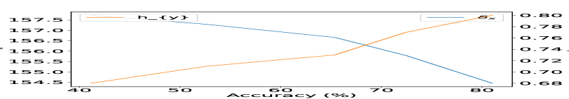
(a) Mettack

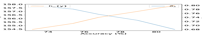
(b) CLGA

Figure 1: Graph homophily $\delta_{x}$ and $h_{y}$ for Cora dataset attacked by Mettack and CLGA with varying attacking powers.

Table I: Number of inserted intra-class links, inserted inter-class links, deleted intra-class links and deleted inter-class links for Mettack and CLGA on Cora dataset.

Attack	Attack power	$5\%$	$10\%$	$15\%$	$20\%$
Mettack	#Inserted intra-class links	$3$	$9$	$14$	$25$
	#Inserted inter-class links	$248$	$486$	$705$	$914$
	#Deleted intra-class links	$2$	$11$	$38$	$68$
	#Deleted inter-class links	$0$	$0$	$3$	$6$
CLGA	#Inserted intra-class links	$18$	$35$	$59$	$77$
	#Inserted inter-class links	$232$	$465$	$690$	$912$
	#Deleted intra-class links	$3$	$5$	$10$	$21$
	#Deleted inter-class links	$0$	$1$	$1$	$3$

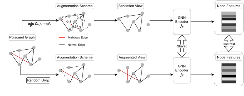
Figure 2: A GCL framework with homophily-driven learnable sanitation view.

In addition, Tab. I shows the number of inserted intra-class links, inserted inter-class links, deleted intra-class links, and deleted inter-class links for Mettack and CLGA at different attacking powers. The results indicate that, for both CLGA and Mettack, the majority of manipulations involve inserting inter-class links into the clean graph. This finding is consistent with the phenomenon presented in Fig. 1. All these experiment results demonstrate that attacks against GCL take effect by reducing the homophily levels of graphs.

V-B Theoretical Analysis

In this section, we provide the theoretical analysis of how the attacks can negatively impact the learning of the GCL model using mutual information as the bridge. For ease of proof, we first introduce a lemma:

Lemma 1 (infoNCE [32]).

The infoNCE object [4] $I_{info}(\cdot)=-\mathcal{L}_{info}(\cdot)$ is the lower bound approximation of the intractable mutual information between the graph and its representations $I(G,\mathbf{Z}=f_{\theta}(G))$.

Then, we provide the theorem to curve the relationship between the graph attacker and the mutual information $I(G,\mathbf{Z})$.

Theorem 1.

The two attacks, Mettack and CLGA, maliciously degenerate the GCL’s performance by minimizing the mutual information between the graph and its representations.

Proof.

We denote the poisoned graph generated by the graph attacker as $G^{p}=\{\mathbf{X},\mathbf{A}^{p}\}$, the corresponding poisoned node embeddings as $\mathbf{Z}^{p}=f_{\theta}(G^{p})$, where $f_{\theta}(\cdot)$ is the GNN encoder. Given the infoNCE object $I_{info}(\cdot)=-\mathcal{L}_{info}(\cdot)$, if $G^{p}$ is generated by CLGA, we have

$$G^{p}=\arg\min_{G}\ I_{info}(t_{1}(G),t_{2}(G)),$$ (7)

since the infoNCE loss is the objective function of CLGA. Then, we have

$$\begin{split}I_{info}(t_{1}(G),t_{2}(G))>I_{info}(t_{1}(G^{p}),t_{2}(G^{p})),\end{split}$$ (8)

based on Lemma 1, we have:

$$\begin{split}I(G,\mathbf{Z}=f_{\theta}(G))>I(G^{p},\mathbf{Z}^{p}=f_{\theta}(G^{p})).\end{split}$$ (9)

If $G^{p}$ is generated by Mettack, we have

$$\begin{split}G^{p}=\arg\max_{G}\ \mathcal{L}_{CE}(\mathbf{Z}^{p},\mathbf{Y}),\end{split}$$ (10)

where $\mathcal{L}_{CE}$ is the cross-entropy loss. We then partition the $\mathcal{L}_{CE}$ as:

$$\begin{split}\mathcal{L}_{CE}&=H(\mathbf{Y})+D_{KL}(p_{Y}\|p_{Z})\\ &=H(\mathbf{Y}|\mathbf{Z})+I(\mathbf{Y},\mathbf{Z})+D_{KL}(p_{Y}\|p_{Z})\\ &=H(\mathbf{Y}|\mathbf{Z})+D_{KL}(p_{YZ}\|p_{Y}p_{Z})+D_{KL}(p_{Y}\|p_{Z}),\end{split}$$ (11)

Next, we build the relationship between mutual information $I(G,\mathbf{Z})$ with the conditional entropy $H(\mathbf{Y}|\mathbf{Z})$ as

$$\begin{split}I(G,\mathbf{Z})&=H(G)-H(G|\mathbf{Z})\\ &=H(G)-H(\mathbf{Y}|\mathbf{Z})+H(\mathbf{Y}|G,\mathbf{Z})-H(G|\mathbf{Y},\mathbf{Z}),\end{split}$$ (12)

Based on Eqn. 11 and 12, we have

$$\begin{split}I(G,\mathbf{Z})=&H(G)-\mathcal{L}_{CE}+D_{KL}(p_{YZ}\|p_{Y}p_{Z})+D_{KL}(p_{Y}\|p_{Z})\\ +&H(\mathbf{Y}|G,\mathbf{Z})-H(G|\mathbf{Y},\mathbf{Z}).\end{split}$$ (13)

Based on Eqn. 13, we observe that the mutual information $I(G,\mathbf{Z})$ is negatively correlated with $\mathcal{L}_{CE}$. Since Mettack can increase the $\mathcal{L}_{CE}$:

$$\begin{split}\mathcal{L}_{CE}(\mathbf{Z},\mathbf{Y})<\mathcal{L}_{CE}(\mathbf{Z}^{p},\mathbf{Y}),\end{split}$$ (14)

then, Eqn. 9 also holds for the poisoned graph generated by Mettack. ∎

Theorem 1 demonstrates that by maliciously altering the graph topology, attacks can decrease the mutual information between the graph data and its representations. On the other hand, GCL’s high-quality node representations are derived from maximizing this mutual information. Therefore, the GCL model may only be able to optimize the mutual information to a sub-optimal level, resulting in the production of low-quality embeddings.

VI Defense Methodology

In this section, we first provide an overview of our framework to clearly describe the whole picture and then clarify our homophily-driven learnable sanitation view for robust graph contrastive learning.

VI-A Overview

In this paper, we propose the homophily-driven learnable sanitation view for enhancing the robustness of unsupervised graph contrastive learning. The proposed model’s overall framework is illustrated in Fig. 2. Similar to the vanilla GCL framework, our model comprises a data augmentation phase and a contrastive learning phase. In the first phase, we introduce a homophily-driven learnable sanitizer that stochastically generates a sanitation view. This learnable sanitizer is parameterized by the link removal probability matrix. In the second phase, the sanitizer generates a sanitation view and contrasts it with the second augmented view, which is produced by random link removal. We then feed these two views to a shared GNN encoder and generate two node features for contrast. Finally, we optimize a homophily-driven objective in an end-to-end manner based on the two node features, updating the link removal probability matrix and the GNN encoder’s parameters via gradient descent.

VI-B End-to-End Design of Learnable Sanitizer

In this section, we introduce our design and implementation of the learnable sanitizer, which can generate sanitation views for GCL. In particular, this sanitizer is seamlessly embedded into the GCL framework and is jointly trained with the contrastive learning process.

VI-B1 Edge-dropping sanitizer

Our design of the sanitizer relies on a stochastic edge-dropping scheme that aims to sanitize the inter-class links injected by the attacker. This design is based on the preliminary experiments (Section V-A) that existing attacks tend to insert inter-class links into the clean graph. Specifically, we use an edge vector $\mathbf{E}$ to represent all the existing edges in a graph. Then, we define a manipulation vector $\mathbf{M}=\{0,1\}^{|\mathbf{E}|}$ that follows the Bernoulli distribution parameterized by $\mathbf{P}$; that is $\mathbf{M}\sim Ber(\mathbf{P})$. For a particular entry $\mathbf{M}_{e}$, we will remove the corresponding edge $e$ if $\mathbf{M}_{e}=1$, which is controlled by the probability $\mathbf{P}_{e}$. Now, the sanitizer can be regarded as a mapping $\mathcal{T}_{\mathbf{P}}(\mathbf{E})\rightarrow\mathbf{E}_{\mathcal{S}}$ parameterized by $\mathbf{P}$, which takes a graph with edge vector $\mathbf{E}$ as input and produce a sanitized view $\mathbf{E}_{\mathcal{S}}$. Formally, we have:

$$\begin{split}\mathbf{E}_{\mathcal{S}}=\mathcal{T}_{\mathbf{P}}(\mathbf{E})\triangleq\mathbf{E}\odot(\mathbf{1}_{|\mathbf{E}|}-\mathbf{M}),\ \ \mathbf{M}\sim Ber(\mathbf{P}),\end{split}$$ (15)

where $\odot(\cdot)$ is the element-wise product operation, $\mathbf{1}_{|\mathbf{E}|}$ is an all-one vector with length equal to the edge number ${|\mathbf{E}|}$, $\mathbf{P}=\{p_{e}\}_{e=1}^{|\mathbf{E}|}$ is the parameters of the sanitizer.

Thus, the remaining task amounts to choosing the proper parameters $\mathbf{P}$ for the sanitizer $\mathcal{T}_{\mathbf{P}}$ so that the generated sanitation views can facilitate contrastive learning to achieve adversarial robustness. Next, we show how to learn the parameters $\mathbf{P}$.

VI-B2 End-to-end learning

The key challenges to learning $\mathcal{T}_{\mathbf{P}}$ are two-fold: choosing the proper objective to guide learning, and integrating learning into the framework of GCL. In this paper, we design the objective function as follows (while deferring the explanation to the next section):

$$\begin{split}\min_{\mathbf{P}\in\mathcal{S}_{1},\theta}\ &\mathcal{L}=\mathcal{L}_{info}(f_{\theta}(\mathbf{E}_{\mathcal{S}}),f_{\theta}(t_{\mathcal{R}}(\mathbf{E})))+\eta\operatorname{Tr}(\mathbf{X}^{\top}\mathbf{L}_{\mathcal{S}}\mathbf{X}),\\ &\text{s.t.}\ \mathbf{E}_{\mathcal{S}}=\mathbf{E}\odot(\mathbf{1}_{|\mathbf{E}|}-\mathbf{M}),\ \mathbf{M}\sim Ber(\mathbf{P}),\\ &\quad\ t_{\mathcal{R}}(\mathbf{E})\in\mathcal{T}_{\mathcal{R}},\ \mathbf{L}_{\mathcal{S}}=\mathbf{I}-\tilde{\mathbf{D}}_{\mathcal{S}}^{-\frac{1}{2}}(\mathbf{A}_{\mathcal{S}}+\mathbf{I})\tilde{\mathbf{D}}_{\mathcal{S}}^{-\frac{1}{2}},\end{split}$$ (16)

where the first view $\mathbf{E}_{\mathcal{S}}$ is the sanitation view generated from the sanitizer, the second view $t_{\mathcal{R}}(\mathbf{E})$ is generated from typical random augmentation scheme $\mathcal{T}_{R}$ that will randomly drop edges with a fixed probability, $\operatorname{Tr}()$ represents the trace of a matrix and $\mathbf{S}_{1}$ is a constrained space of the sanitation operation with $\epsilon$ controlling the sanitation degree:

$$\begin{split}\mathbf{S}_{1}=\{s|s\in[0,1]^{E},\|s\|_{1}\leq\epsilon\}.\end{split}$$ (17)

$\mathbf{L}_{\mathcal{S}}$ is the graph Laplacian based on the sanitation view $\mathbf{E}_{\mathcal{S}}$.

In our design, the training objective of the sanitizer is embedded into that of the GCL. That is, we train the sanitizer together with the contrastive learning, using a hyperparameter $\eta$ to control the relative importance of optimizing the infoNCE loss and the graph homophily $\delta_{x}$. Then, the learnable sanitizer sample the sanitation view $\mathbf{E}_{\mathcal{S}}$ based on Eqn. 15 for each iteration. After that, the shared GNN encoder $f_{\theta}(\cdot)$ converts the graph data from the two views to low-dimensional node embedding matrices and obtain the training loss $\mathcal{L}$. During the backward pass, we compute the gradient of $\mathcal{L}$ with respect to the parameters $\mathbf{P}$ and $\theta$ and update them via gradient descent.

VI-B3 Insights behind our design

The objective function of our robust model in Eqn. 16 contains two vital components: the infoNCE loss over two views and the graph homophily measurement $\delta_{x}=\operatorname{Tr}(\mathbf{X}^{\top}\mathbf{LX})$. In Sec. V-B, it was (Theorem 1) shown that the attacks would degrade the consistency (mutual information) between the graph and its representations, leading to a decrease in the quality of node embeddings. Therefore, an effective robust model should restore the properties distorted by malicious topology manipulations, acting as a countermeasure against the graph attacker. To achieve this, the sanitizer should be designed in a way that the mutual information between graph and representation is preserved. As the infoNCE objective is a common approximation to the intractable mutual information, we optimize the sanitation view to minimize the infoNCE loss (i.e., maximize the mutual information). There are other graph sanitation frameworks for GNNs, such as those proposed in [33, 34], which adopt the cross-entropy loss as the objective for sanitation. However, these are infeasible in an unsupervised learning setting as they require access to node labels for training. Nevertheless, we want to emphasize that we are the first to theoretically describe the inherent relationship between the objective of the GCL model and the graph attacks, which provides strong insights for learning the sanitation view.

Furthermore, as discussed in Sec. V-A, it has been observed that attacks (Mettack and CLGA) tend to add heterophilous links, which can decrease the homophily degree of the graph (e.g., increasing $\delta_{x}$). Based on this observation, we choose the graph homophily metric $\delta_{x}$ as a second supervision term to sanitize the poisoned graph to obtain the sanitation view. Compared to $h_{y}$, which requires node labels, $\delta_{x}$ does not, and is thus suitable for unsupervised learning. In Sec. VII, we provide a comprehensive ablation study to verify the significance of these two components.

VI-C Implementation

Now, we introduce several techniques to efficiently solve the optimization problem (16).

VI-C1 Gumbel-Softmax Re-parametrization

To optimize the parameters $\mathbf{P}$ via gradient descent, it is necessary to tackle the in-differentiation of the sampling procedure in Eqn. 15 during the backward pass. To tackle this problem, we utilize the Gumbel-Softmax re-parametrization technique [19] to relax the discrete Bernoulli sampling procedure to a differentiable Bernoulli approximation. Using the relaxed sample, we implement the straight-through estimator [20] to discretize the relaxed samples in the forward pass and set the gradient of discretization operation to $1$, i.e., the gradients are directly passed to the relaxed samples rather than the discrete values. Hence, we reconstruct the mapping from $\mathbf{P}$ to $\mathbf{M}$ as:

$$\begin{split}\mathbf{M}_{e}=\lfloor\frac{1}{1+e^{-(\log\mathbf{P}_{e}+g)/\tau}}+\frac{1}{2}\rceil,\end{split}$$ (18)

where $\lfloor\cdot\rceil$ is the rounding function, $g\sim Gumbel(0,1)$ is a standard Gumbel random variable with zero mean and the scale equal to $1$. Then, we can reformulate Eqn. 15 to:

$$\begin{split}&\mathbf{E}_{\mathcal{S}}=\mathbf{E}\odot(\mathbf{1}_{|E|}-\lfloor\frac{1}{1+e^{-(\log\mathbf{P}+g)/\tau}}+\frac{1}{2}\rceil),\\ &\text{where}\ \mathbf{P}\in\mathcal{S}_{1}=\{\mathbf{P}_{e}|\sum_{e}\mathbf{P}_{e}\leq\epsilon,\mathbf{P}_{e}\in[0,1]\ \forall e\in\{1,..,E\}\}.\end{split}$$ (19)

VI-C2 Projection Gradient Descent

Formally, to optimize the parameters $\mathbf{P}$ under the constraint $\mathcal{S}_{1}$ defined in Eqn. 19, we deploy the projection gradient descent to optimize the relaxed constrained optimization problem introduced in Eqn. 19:

$$\begin{split}\mathbf{P}^{(t)}=\text{Proj}_{\mathcal{S}_{1}}(\mathbf{P}^{(t-1)}-\alpha\nabla_{\mathbf{P}^{(t-1)}}\mathcal{L}(t_{1}(\mathcal{G}),t_{2}(\mathcal{G}),\theta))\end{split}$$ (20)

at the $t$-th iteration, where $\alpha$ is the learning rate of the projection gradient descent, $\nabla_{\mathbf{P}}\mathcal{L}(t_{1}(\mathcal{G}),t_{2}(\mathcal{G}),\theta)$ denotes the gradient of the loss defined in Eqn. 16, $\text{Proj}_{\mathcal{S}_{1}}$ is the projection operator to project the updated parameters to satisfy the constraint. Referring to [35], the projection operator $\text{Proj}_{\mathcal{S}_{1}}$ has the closed-form solutions:

$$\begin{split}\text{Proj}_{\mathcal{S}_{1}}(\mathbf{P})=\begin{cases}\text{Proj}_{[0,1]}[\mathbf{P}-\mu\mathbf{1}_{E}],&\mbox{if }\mu>0\mbox{ and }\\ &\sum_{e}\text{Proj}_{[0,1]}[\mathbf{P}-\mu\mathbf{1}_{E}]=\epsilon,\\ \\ \text{Proj}_{[0,1]}[\mathbf{P}],&\mbox{if }\sum_{e}\text{Proj}_{[0,1]}[\mathbf{P}]\leq\epsilon,\end{cases}\end{split}$$

where $\text{Proj}_{[0,1]}[\mathbf{P}]$ clips the parameters vector $\mathbf{P}$ into the range $[0,1]$. The bisection method [36] is used over $\mu\in\{\min(\mathbf{P}-\mathbf{1}_{E}),\max(\mathbf{P})\}$ to find the solution to $\sum_{e}\text{Proj}_{[0,1]}[\mathbf{P}-\mu\mathbf{1}_{E}]=\epsilon$ with the convergence rate $\log_{2}[(\max(\mathbf{P})-\min(\mathbf{P}-\mathbf{1}_{E}))/\xi]$ with $\xi$-error tolerance [37].

VI-D Unsupervised Hyperparameter Tuning

One issue that remains unsolved is the tuning of the hyperparameter $\eta$. While some previous works [6, 5, 4] use node labels for tuning hyperparameters, we consider a strict unsupervised setting where node labels are not available during training and are only used in the downstream node classification task for testing. We thus propose a fully unsupervised method to tune the parameter $\eta$.

In Sec. III-C, we introduced the normalized cut loss in Eqn. 2, which counts the number of inter-cluster links within a given graph. The loss value depends on the quality of the clustering result determined by cluster assignment matrix $\mathbf{C}$. We propose to use this normalized cut loss as the supervision for searching the parameter $\eta$. The intuition is that if the generated node embeddings have high quality, the clustering result should be accurate, leading to a low loss value. In fact, several previous works [38, 28] have utilized this loss as supervision in different ways.

Following this intuition, we use the normalized cut loss as a metric to quantify the quality of node embedding and tune $\eta$ by monitoring this loss during training. Specifically, during the $t$-th iteration, we obtain the sanitized adjacency matrix $\mathbf{A}_{\mathcal{S}}^{(t)}$ (corresponding with $\mathbf{E}_{\mathcal{S}}^{(t)}$ in Eqn. (19)). Then we feed it into a two-layered GNN encoder to the sanitized node embeddings $\mathbf{H}_{\mathcal{S}}^{(t)}=f_{\theta}(\mathbf{A}_{\mathcal{S}}^{(t)},\mathbf{X})$ from Eqn. 1 and get the pseudo normalized cut loss:

$$\begin{split}\mathcal{L}_{pnc}^{(t)}=\operatorname{Tr}((\sigma(\mathbf{H}_{1}^{(t)})^{\top}\mathbf{L}^{(t)}\sigma(\mathbf{H}_{1}^{(t)}))\oslash(\sigma(\mathbf{H}_{1}^{(t)})^{\top}\mathbf{D}^{(t)}\sigma(\mathbf{H}_{1}^{(t)})),\end{split}$$

where $\sigma(\cdot)$ is the sigmoid function. $\mathcal{L}_{pnc}$ is time-efficient since it does not require additional models or parameters to be trained. We use the early-stopping trick [39] to effectively tune the hyperparameter $\eta$. That is,

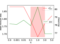
Figure 3: $\mathcal{L}_{pnc}^{t^{*}}$ v.s. Accuracy.

we record the value of $\mathcal{L}_{pnc}^{(t)}$ for each iteration during training and select the model with the minimum $\mathcal{L}_{pnc}$ as our final result for evaluation. We denote the best metric as $\mathcal{L}_{pnc}^{t^{*}}$. Fig. 3 presents the values of $\mathcal{L}_{pnc}^{t^{*}}$ and node classification accuracy with varying $\eta$. The results indicate that in most cases $\mathcal{L}_{pnc}^{t^{*}}$ is negatively related to the node classification accuracy, especially when the value of $\mathcal{L}_{pnc}^{t^{*}}$ falls into the neighborhood of the minimum value, i.e., $\eta\in[0.1,3]$ (the Pearson correlation coefficients $r(\mathcal{L}_{pnc}^{t^{*}},accuracy)=-0.89$). This phenomenon demonstrates that it is reasonable to tune $\eta$ via searching for the best $\mathcal{L}_{pnc}^{t^{*}}$, since the GCL model that achieves the minimum $\mathcal{L}_{pnc}^{t^{*}}$ is likely to get the best accuracy. The algorithm of our work is in Alg. 1.

Input: Poisoned graph $\mathcal{G}=\{\mathbf{E},\mathbf{X}\}$, $\eta$.

Parameters: Sanitation probability $\mathbf{P}$, GNN encoder $f_{\theta}(\cdot)$ with weight matrices $\theta=\{\mathbf{W}^{(1)},\mathbf{W}^{(2)}\}$.

Output: Sanitized node embeddings matrix $\mathbf{H}_{1}$.

1:  Let $t=0$, initialize parameters $\mathbf{P}=\mathbf{P}^{0}$, $\theta=\theta^{0}$.

2:  while $t\leq T$ do

3:     Sample $g\sim Gumbel(0,1)$.

4:     Sample sanitation view $\mathcal{G}_{1}^{t}$ from $\mathbf{E}_{\mathcal{S}}^{t}=\mathbf{E}\odot(\mathbf{1}_{E}-\lfloor\frac{1}{1+e^{-(\log\mathbf{P}^{t}+g)/\tau}}+\frac{1}{2}\rceil)$.

5:     Sample another view $\mathcal{G}_{2}^{t}$ by randomly dropping links.

6:     Compute graph Laplacian $\mathbf{L}^{t}=\mathbf{I}-(\tilde{\mathbf{D}}^{t})^{-\frac{1}{2}}\tilde{\mathbf{A}}^{t}(\tilde{\mathbf{D}}^{t})^{-\frac{1}{2}}$.

7:     Compute loss $\mathcal{L}=\mathcal{L}_{info}(\mathcal{G}_{1}^{t},\mathcal{G}_{2}^{t})+\eta\operatorname{Tr}(\mathbf{X}^{\top}\mathbf{L}^{t}\mathbf{X})$.

8:     Projection gradient descent and update $\mathbf{P}^{t}$ from Eqn. 20.

9:     Gradient descent and update $\theta^{t}$ based on $\mathcal{L}$.

10:     Compute pseudo normalized cut loss $\mathcal{L}_{pnc}^{t}$ from Eqn. VI-D.

11:  end while

12:  Get the best iteration $t^{*}$ with the minimum value $\mathcal{L}_{pnc}^{t^{*}}$.

13:  return  Sanitized node embeddings $\mathbf{H}_{1}=f_{\theta^{t^{*}}}(\mathbf{A}^{t^{*}},\mathbf{X})$.

Algorithm 1 GCHS

VII Experiments

In this section, we introduce the experimental settings and conduct comprehensive experiments to validate the effectiveness of our robust model. Specifically, we outline the questions that we seek to answer below.

• RQ1: Comparing with baseline models, does our model achieve better robust performance for node classification and graph clustering downstream tasks?

• RQ2: How do different components of the model contribute to its performance?

• RQ3: How do the hyperparameters in the proposed model impact the quality of the node embeddings?

VII-A Experimental settings

VII-A1 Datasets

We use six popular benchmark graph datasets: Cora, CiteSeer, Cora-ML, Photo, Computers and WikiCS [10, 40, 41] for evaluation. The detailed statistics of these datasets are summarized in Tab. II.

Table II: Dataset statistics.

Datasets	#Nodes	#Edges	#Classes	#Features
Cora	$2708$	$5278$	$7$	$1433$
Citeseer	$3327$	$4552$	$6$	$3703$
Cora-ML	$2995$	$8416$	$7$	$2879$
Photo	$7650$	$119081$	$8$	$745$
Computers	$13752$	$245861$	$10$	$767$
WikiCS	$11701$	$215863$	$10$	$300$

VII-A2 Settings

To validate the quality of the node embeddings effectively, we utilize semi-supervised node classification and unsupervised graph clustering as downstream tasks. For node classification, we train a multi-class logistic regression model with Adam optimizer [42] and randomly split the node labels into three groups: training, validation and testing set with the ratio as $10\%$, $10\%$ and $80\%$. For graph clustering, the K-means clustering [43] algorithm is run based on the pre-trained node embeddings derived from GCL models and we report the normalized mutual information (NMI) to quantify the robustness of the graph clustering performances. A two-layered GNN encoder is deployed for all the GCL models. The embedding dimension of the first layer is $128$ for all the datasets and the embedding dimension of the second layer is $32$ for Cora, CiteSeer and Cora-ML and $128$ for Photo, Computers and WikiCS. We train the GNN encoder parameters $\theta$ via Adam optimizer with the learning rate equal to $0.0005$ and the training epochs equal to $1000$. We run all the models $10$ times with different seeds and report the mean value for a fair comparison. The hyperparameter $\eta$ based on $\mathcal{L}_{pnc}^{*}$ in Eqn. VI-D without querying the node labels. All the models are executed on an Intel 10C20T Core i9-10850K CPU with GIGABYTE RTX3090 24GB GPU.

Table III: Performances on node classification against Mettack.

Dataset	$\frac{B}{|E|}$	BGRL	DGI	MVGRL	GRACE	ARIEL	GCA	SPAN	GCHS
Cora	0%	75.12(1.7)	81.04(1.7)	82.93(0.8)	81.02(1.17)	81.14(0.87)	82.09(0.36)	81.83(0.88)	80.03(0.78)
	5%	66.97(1.4)	73.41(1.0)	75.73(0.5)	72.46(1.80)	74.92(1.23)	73.80(1.09)	74.18(0.94)	78.78(1.02)
	10%	60.11(1.7)	68.03(1.8)	71.10(1.4)	65.37(2.80)	71.93(1.24)	70.26(1.34)	68.81(1.89)	75.93(0.85)
	15%	51.85(3.0)	59.70(2.7)	64.69(1.9)	52.62(3.10)	52.91(4.39)	57.89(1.52)	58.44(3.23)	71.89(1.56)
	20%	44.18(4.3)	51.43(2.3)	57.29(2.8)	41.17(3.98)	43.71(3.87)	46.03(3.01)	45.71(2.50)	68.81(2.44)
CiteSeer	0%	62.55(1.4)	70.63(1.3)	72.35(0.8)	70.97(1.14)	71.72(1.26)	72.37(1.06)	71.61(0.96)	71.80(1.28)
	5%	56.90(2.7)	66.43(1.1)	68.93(0.9)	69.55(1.96)	70.79(1.70)	67.93(1.14)	69.08(1.32)	70.93(1.27)
	10%	52.30(2.6)	60.78(2.8)	65.01(1.2)	63.49(2.25)	69.14(2.14)	60.82(1.26)	65.18(2.58)	69.43(1.28)
	15%	44.44(2.7)	53.30(2.4)	58.51(1.3)	53.67(2.73)	56.46(2.33)	52.52(1.67)	56.08(3.50)	65.84(1.16)
	20%	40.89(3.2)	49.54(1.9)	51.69(1.6)	47.62(2.95)	47.93(3.17)	48.79(1.42)	50.68(3.02)	62.65(1.48)
Cora-ML	0%	74.74(1.3)	81.93(0.9)	82.93(0.9)	82.46(0.54)	82.68(0.44)	82.78(0.76)	82.03(0.67)	81.41(0.75)
	5%	64.26(1.9)	67.06(2.9)	70.18(2.5)	68.65(1.96)	71.21(1.74)	69.84(1.74)	69.34(0.88)	77.90(0.83)
	10%	53.08(2.6)	49.34(2.1)	54.20(2.4)	50.49(1.72)	51.87(1.76)	46.81(1.86)	50.44(1.22)	71.57(1.66)
	15%	44.09(3.6)	42.21(1.5)	45.96(3.3)	40.89(3.40)	41.11(2.31)	37.17(3.58)	41.77(2.37)	64.56(1.82)
	20%	37.41(3.3)	34.35(0.4)	37.40(2.3)	31.57(3.28)	28.52(2.22)	26.69(2.10)	33.46(2.47)	56.43(2.50)
Photo	0%	85.79(0.4)	78.26(0.5)	89.48(0.8)	90.16(0.2)	89.39(0.7)	89.19(0.9)	87.53(1.0)	90.87(0.3)
	5%	66.50(2.8)	62.24(3.4)	73.14(1.3)	70.87(1.1)	69.85(2.4)	76.45(2.1)	72.46(2.3)	78.37(2.2)
	10%	52.62(3.9)	47.76(3.7)	58.63(3.3)	51.39(1.5)	53.92(1.8)	60.57(2.0)	63.46(0.4)	67.80(2.4)
	15%	43.56(2.4)	40.73(3.6)	49.82(2.0)	44.37(1.6)	45.98(1.8)	51.66(1.4)	50.02(0.4)	59.19(1.5)
	20%	35.68(3.5)	37.91(4.0)	45.00(2.0)	32.45(1.4)	34.19(1.8)	45.35(1.3)	46.81(3.4)	54.68(2.9)
Computers	0%	77.32(1.6)	72.88(2.9)	80.03(0.6)	84.30(0.8)	83.83(1.4)	85.02(1.2)	80.87(0.8)	83.99(1.1)
	5%	63.12(1.3)	63.91(1.9)	69.16(0.6)	66.22(1.0)	67.51(1.7)	68.02(0.9)	64.06(1.4)	72.25(2.2)
	10%	61.33(2.1)	57.06(1.9)	64.58(0.4)	58.07(2.0)	57.04(1.5)	58.90(2.1)	54.81(1.3)	66.14(2.1)
	15%	52.59(3.4)	51.40(2.0)	54.99(2.6)	52.58(2.1)	43.65(2.6)	52.90(2.6)	45.63(3.2)	59.93(3.8)
	20%	37.61(2.3)	41.54(4.9)	44.98(3.5)	37.21(3.9)	34.71(1.7)	38.81(3.6)	37.39(2.1)	51.13(4.1)
WikiCS	0%	74.78(0.5)	77.09(0.8)	78.42(0.4)	79.70(0.2)	78.48(0.5)	79.35(0.3)	79.27(0.4)	78.02(0.3)
	5%	40.91(1.0)	43.71(2.2)	42.17(1.8)	41.30(1.1)	43.92(1.0)	41.67(0.8)	40.60(1.1)	55.93(0.8)
	10%	29.93(0.9)	33.88(2.7)	30.73(0.7)	30.89(1.1)	33.55(1.4)	31.18(0.7)	28.48(0.7)	49.30(0.6)
	15%	24.35(0.7)	27.10(2.0)	24.54(1.1)	25.40(0.4)	27.37(0.6)	25.25(0.5)	23.32(0.7)	42.96(1.1)
	20%	21.60(1.8)	23.79(1.3)	22.38(0.8)	23.23(0.4)	24.56(0.7)	23.03(0.7)	21.79(0.5)	36.47(1.0)

Table IV: Performances on node classification against CLGA.

Dataset	$\frac{B}{|E|}$	BGRL	DGI	MVGRL	GRACE	ARIEL	GCA	SPAN	GCHS
Cora	5%	70.78(1.1)	78.96(1.3)	80.09(0.9)	78.95(0.93)	78.47(0.72)	78.55(0.72)	78.96(0.72)	79.13(0.59)
	10%	68.35(1.9)	75.64(1.2)	77.92(0.9)	76.79(1.35)	76.31(0.92)	77.15(0.78)	77.22(1.09)	78.62(1.11))
	15%	66.15(1.3)	73.72(0.7)	75.89(1.0)	75.38(1.14)	74.75(0.89)	74.71(1.15)	76.11(1.19)	78.18(1.02)
	20%	64.44(1.8)	71.94(1.7)	74.64(0.8)	73.13(1.06)	74.44(1.19)	71.78(1.00)	74.43(1.64)	76.82(1.16)
CiteSeer	5%	58.52(1.3)	66.24(1.5)	68.60(1.2)	69.38(1.22)	70.43(1.17)	67.92(1.04)	70.38(1.11)	71.18(1.22)
	10%	56.27(1.3)	65.62(1.5)	67.65(1.0)	67.80(1.04)	69.25(2.09)	65.43(1.07)	68.74(1.34)	70.11(0.86)
	15%	54.09(2.0)	63.75(1.6)	66.29(0.8)	67.52(1.55)	66.77(2.40)	62.43(1.74)	67.71(1.33)	69.58(1.54)
	20%	51.24(1.9)	62.55(1.5)	64.24(1.3)	65.68(1.65)	64.99(2.06)	60.52(1.66)	66.62(1.36)	67.90(1.12)
Cora-ML	5%	70.38(2.1)	77.91(0.9)	78.62(0.8)	79.16(0.99)	79.27(0.64)	77.53(0.70)	79.36(0.98)	80.02(0.82)
	10%	68.75(1.7)	76.40(1.1)	76.29(0.9)	77.34(1.01)	77.87(0.66)	76.18(0.88)	77.96(0.82)	78.68(0.90)
	15%	67.38(1.1)	75.46(1.4)	74.61(0.6)	76.54(0.83)	76.97(0.90)	74.09(1.15)	77.10(0.56)	77.34(0.92)
	20%	65.09(2.0)	73.42(1.7)	73.40(0.8)	75.36(0.80)	75.36(1.28)	72.54(0.89)	75.99(0.52)	76.72(0.79)
Photo	5%	80.79(1.4)	75.80(2.8)	84.86(0.7)	81.91(0.8)	82.28(1.0)	82.25(1.1)	84.18(0.8)	87.09(0.6)
	10%	79.11(1.0)	72.74(3.4)	82.27(0.9)	77.49(1.0)	78.12(0.9)	79.17(0.8)	82.21(0.7)	85.04(0.5)
	15%	77.83(0.9)	68.99(0.5)	80.39(0.7)	75.28(1.0)	76.98(0.6)	76.68(0.8)	80.78(0.5)	82.11(1.1)
	20%	76.97(0.8)	68.59(2.0)	78.88(0.8)	71.85(1.2)	74.92(1.3)	73.10(0.7)	78.90(0.9)	79.21(2.2)

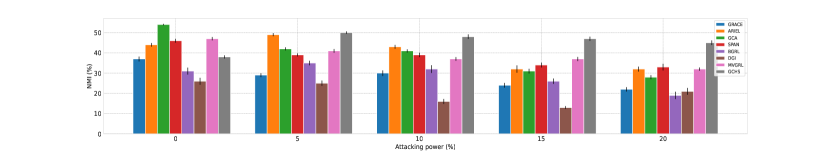
(a) Cora

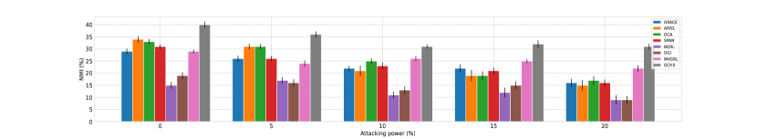
(b) CiteSeer

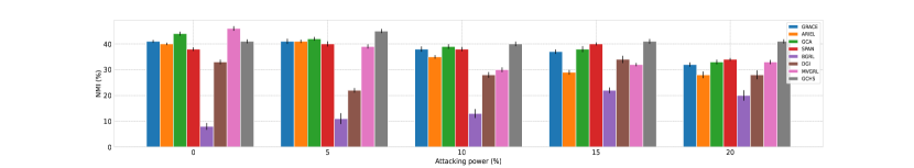
(c) Cora-ML

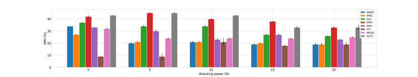
(d) Photo

Figure 4: Performances on graph clustering.

VII-A3 Baseline Models

To thoroughly validate the robustness of our proposed method, we have conducted a comparative analysis with several state-of-the-art graph contrastive learning models: BGRL [26], DGI [25], MVGRL [24], GRACE [3], GCA [4], ARIEL [5], and SPAN [6]. Among them, ARIEL and SPAN are known for their robustness in GCL. To ensure a rigorous comparison, we have used the same hyper-parameter settings as reported in the corresponding literature, where all the baselines are fine-tuned based on the performance of the validation set.

VII-B Robustness on Node Classification

The objective of this paper is to examine the adversarial robustness of our proposed model against two common graph structural attacks: Mettack [12] (a graph structural attack with GNN as its surrogate model) and CLGA [13] (a graph structural attack with GCL as its surrogate model).

VII-B1 Against Mettack

Tab. III displays the accuracies of various GCL models for the semi-supervised node classification under different attacking powers. In particular, the attacking power is defined as the percentage $\frac{B}{|E|}$, where $B$ is the attack budget (number of modified edges) and $|E|$ is the total edge number of the clean graph. To cover most attacking scenarios, we have chosen the attacking power from $\{5\%,10\%,15\%,20\%\}$, which is consistent with the prior literature [12, 13].

The results in Tab. III indicate that Mettack affects all GCL methods, although it is originally designed to attack vanilla GNNs. This is because the GCL models also rely on the GNN encoder to convert the graph data into low-dimensional embeddings, and thus, Mettack can indirectly compromise the quality of the GCL’s node embeddings.

The second observation is that our proposed model outperforms the other baselines across various levels of attacking power. Moreover, the performance gap between our model and other baselines widens as the attacking power grows from $5\%$ to $20\%$. For example, on the Cora dataset, the performance gaps between our model with GRACE, ARIEL, GCA, SPAN, BGRL, DGI and MVGRL are $8.02\%$, $4.90\%$, $6.32\%$, $5.84\%$, $14.99\%$, $6.82\%$ and $3.87\%$ when the attacking power is $5\%$. The corresponding margins under $20\%$ attacking power are $40.17\%$, $36.47\%$, $33.11\%$, $33.57\%$, $35.79\%$, $25.26\%$, $16.74\%$. This can be attributed to the fact that as the attacking power grows, more malicious heterophilous links are inserted. However, the sanitizer in our proposed model can effectively eliminate a greater number of malicious edges from the heavily poisoned graph, thereby improving the quality of node embeddings and making them more distinguishable across different classes.

Thirdly, it is observed that in certain scenarios, our model cannot surpass other strong baselines on clean graphs. For instance, on the CiteSeer dataset, the node classification accuracy of our model is slightly lower than that of GCA and MVGRL by $0.57\%$ and $0.55\%$. This phenomenon is common in the field of adversarial machine learning and can be attributed to the trade-off between expressive power and the robustness of the model [44, 45].

VII-B2 Against CLGA

Tab. IV presents the robustness of various GCL models under the unsupervised attack CLGA. Similar to its performance under Mettack, our model outperforms other baselines across various levels of attacking power. However, since CLGA is an unsupervised attack, the degree of decreasing node classification accuracy for GCL models is not as significant as in Mettack, which specifically targets the test set.

We note that MVGRL performs well against CLGA and even outperforms our method when the attacking power is equal to $5\%$ on the Cora dataset. This is because MVGRL does not use the infoNCE loss for training, which is the attack objective of CLGA. Nevertheless, our model outperforms MVGRL on the Cora dataset when the attacking power is larger or equal to $10\%$. Overall, the proposed homophily-driven learnable sanitation view effectively promotes the robustness of the vanilla GCL framework by automatically detecting and pruning potential heterophilous edges in the poisoned graph, as demonstrated by the robust performance results shown in Tab. III and Tab. IV.

VII-C Robustness on Graph Clustering

In this section, we examine the adversarial robustness of GCL models on the graph clustering downstream task, with a focus on the unsupervised graph structural attack method CLGA. This attack method is particularly relevant since it can significantly degrade the quality of node embeddings, irrespective of the downstream task. The attacking scenario is the same as described in Section VII-B, and the experiment results are presented in Fig. 4.

Firstly, we investigate the attack performance of CLGA against the graph clustering task by observing the degeneration percentage of GCA’s clustering performance (CLGA chooses GCA as its representative surrogate model). It is observed that for the four graph data listed in Fig. 4, the NMI score of the GCA model indeed decreases as the graph attacker increases the attacking power. For example, compared to the clean graph, the decreasing percentages on the poisoned Cora dataset are $22.22\%$, $24.07\%$, $37.04\%$, $40.74\%$ when the attacking power increases from $5\%$ to $20\%$. This phenomenon demonstrates that CLGA can successfully attack the graph clustering task by indirectly attacking the infoNCE loss of the graph contrastive learning framework.

The second key finding is that our proposed model achieves the best performance in most cases with various attacking powers ranging from $5\%$ to $20\%$. For instance, under the attacking power equal to $10\%$, our method outperforms GCA and SPAN around $19.35\%$ and $25.81\%$ for CiteSeer. Similar to the node classification task, our method cannot achieve the best clustering performance on the clean graph. This bottleneck is still due to the trade-off between the expressive power and the robust model. Alternatively, SPAN can perform well in certain scenarios and even outperform our method on the Photo data when the attacking power is equal to $15\%$ demonstrating that SPAN has intrinsic robustness property on the graph clustering task. The reason is that the spectrum-invariance-based augmentation of SPAN can inherently preserve the clustering consistency to some extent. Specifically, the graph spectrum is a summary of graph structural properties such as clustering [46, 47]. SPAN enhances the robustness of graph clustering by selecting two augmentation views to simultaneously maximize and minimize the spectrum distance of the original graph and corrupted graph in the augmentation view while maintaining consistency on the embedding space between the two augmentation views from the contrastive loss. However, the fact that our method performs better than SPAN in most cases demonstrates that the homophily-driven sanitation view of sanitizing the potential inter-class links is a more appropriate defense method to promote the robustness of the graph clustering task.

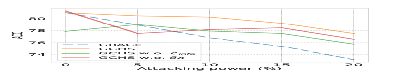
(a) CLGA

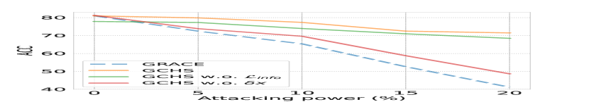
(b) Mettack

Figure 5: Ablation study of two model variants.

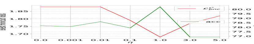
(a) CLGA

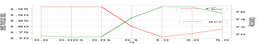
(b) Mettack

Figure 6: Sensitivity analysis on $\eta$.

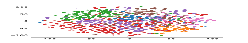
(a) GCHS-CLGA

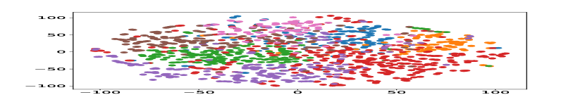
(b) GCHS-Mettack

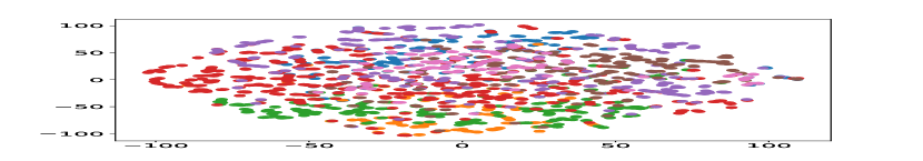
(c) SPAN-CLGA

(d) SPAN-Mettack

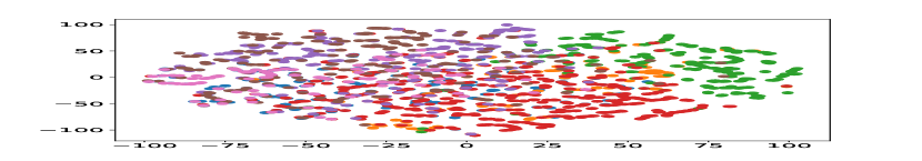
(e) ARIEL-CLGA

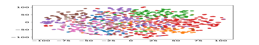
(f) ARIEL-Mettack

Figure 7: Scatterplots for GCHS, SPAN and ARIEL.

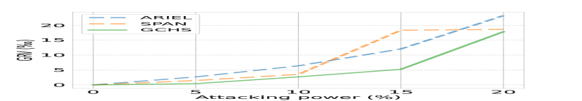
(a) CLGA

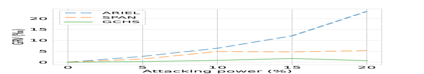
(b) Mettack

Figure 8: Performances on GRV.

VII-D Ablation Study

In Sec. VI-B3, we concluded that both infoNCE loss and the graph homophily $\delta_{x}$ can serve as appropriate supervisors and lead to high-quality sanitized node embeddings. In this section, we present the ablation study to verify the effectiveness of these two vital components. Particularly, we introduce two model variants as follows:

• GCHS w.o. $\mathcal{L}_{info}$: we remove the infoNCE loss in Eqn. 16 and first train the sanitation view to optimize $\delta_{x}$. Then, we train the GCL model with the pre-trained sanitation view.

• GCHS w.o. $\delta_{x}$: we remove the $\delta_{x}$ term in Eqn. 16 and only optimize the infoNCE loss in GCHS.

The results are presented in Fig. 5. Firstly, comparing the robust performance of GCHS w.o. $\mathcal{L}_{info}$, GCHS w.o. $\delta_{x}$ and GRACE, we find out that both optimizing the infoNCE loss and the graph homophily $\delta_{x}$ can enhance the robustness of the GCL model since in most cases the two model variants outperform GRACE. Secondly, the comparison of GCHS w.o. $\mathcal{L}_{info}$ and GCHS w.o. $\delta_{x}$ under Mettack reveals that optimizing $\delta_{x}$ provides more powerful robustness than optimizing $\mathcal{L}_{info}$. The reason is that Mettack will maliciously inject more inter-class links than CLGA and directly optimizing the graph homophily will have a more significant sanitation gain than indirectly optimizing the task-related loss function. Thirdly, the observation that GCHS outperforms both model variants demonstrate that considering both components is necessary to achieve the best sanitized node embeddings.

VII-E Sensitivity Analysis

In this section, we examine the sensitivity of GCHS to the hyperparameter $\eta$ in Eqn. 16. To be specific, we report the best pseudo normalized cut loss $\mathcal{L}_{pnc}^{t^{*}}$ and the node classification accuracy with attack power equal to $10\%$ for CLGA and Mettack as exemplar and present the results in Fig. 6. Moreover, we tune the hyperparameter $\eta$ ranged in $[0,0.0001,0.001,0.01,0.1,1,3,5].$ The experiments demonstrate that too large and too small $\eta$ may lead to sub-optimal performance on GCHS under different attacking scenarios. Alternatively, for all the cases listed in Fig. 6 $\eta=1$ can achieve the minimum $\mathcal{L}_{pnc}^{t^{*}}$ (coincide with the best node classification accuracy).

VII-F Embeddings Visualization

We provide the node embeddings visualization for GCHS, SPAN and ARIEL (robust GCLs) to qualitatively evaluate the quality of node embeddings under different attacking scenarios (CLGA and Mettack with attacking power equal to $20\%$) in Fig. 7. The visualization is depicted on the transformed node embeddings generated by GCHS, SPAN and ARIEL via t-SNE [48]. Clearly, the node embeddings for GCHS are more discriminative than SPAN and ARIEL and the clusters of GCHS are more cohesive than the others.

VII-G Robustness on GRV

To illustrate the robustness of GCHS from an information-theoretic perspective, we utilize GRV [29] mentioned in Definition. 1 to indirectly quantify the GCL’s robustness. It is worth noting that GRV measures the difference between the mutual information of the node embeddings for the clean graph and the poisoned graph. Here we utilize the infoNCE loss to approximate the mutual information. We emphasize that we only use the clean graph’s information on computing GRV instead of training the robust model and hence prevent the information leakage. We compare GCHS with SPAN and ARIEL in this part, and report the GRVs for each robust model in Fig. 8. A lower GRV indicates better robustness. It is observed that GCHS achieves the minimum GRV for both CLGA and Mettack, demonstrating that the node embeddings of GCHS are more robust than those of the other models from an information-theoretic perspective.

VII-H Time Cost

Table V: Time cost (s).

Dataset	BGRL	DGI	MVGRL	GRACE	GCA	ARIEL	SPAN	GCHS
Cora	$0.011$	$0.005$	$0.008$	$0.008$	$0.009$	$0.084$	$0.245$	$0.045$
CiteSeer	$0.017$	$0.006$	$0.011$	$0.010$	$0.009$	$0.068$	$0.174$	$0.041$
Cora-ML	$0.029$	$0.006$	$0.013$	$0.015$	$0.011$	$0.111$	$0.310$	$0.067$
Photo	$0.031$	$0.010$	$0.019$	$0.038$	$0.051$	$1.056$	$4.347$	$0.468$
Computers	$0.059$	$0.023$	$0.031$	$0.099$	$0.090$	$5.198$	$8.694$	$2.293$
WikiCS	$0.043$	$0.018$	$0.026$	$0.067$	$0.066$	$4.085$	$7.394$	$1.360$

Tab. V presents the time required for each iteration of the training phase of the GCL models. The last three columns show the time cost of using the learnable augmentation views. It is evident that the GCL model with learnable augmentation views requires more computation time than the others. In addition to that, our model consumes the least amount of computation time compared to the other two models with learnable augmentation views.

VIII Conclusion

In this paper, we investigate the adversarial robustness of the GCL model in the face of graph structural attacks. This research proposes a novel homophily-driven, learnable sanitation view that enhances the GCL model’s robustness by automatically eliminating potential malicious edges in the augmentation view, which is based on the assumption that an attacker would aim to disrupt the homophily degree and the mutual information of the clean graph. To this end, we choose the objective as the weighted sum of the infoNCE loss with the graph homophily $\delta_{x}$ to jointly optimize the parameters in the sanitation view and GNN encoder. The Gumbel-Softmax re-parametrization technique is employed to overcome the non-differentiable mapping issue during the sampling phase, while the parameters in the sanitation view are optimized via projection gradient descent. Besides, we novelly craft a pseudo normalized cut loss to easily determine the best choice of the hyperparameter $\eta$ without avoiding the unsupervised setting of the GCL framework during training. Extensive experiments demonstrate that our method can prominently boost the robustness of the GCL model.

References

- [1] A. Grover and J. Leskovec, “Node2vec: Scalable feature learning for networks,” in Proceedings of the 22nd ACM SIGKDD International Conference on Knowledge Discovery and Data Mining, KDD ’16, (New York, NY, USA), p. 855–864, Association for Computing Machinery, 2016.
- [2] B. Perozzi, R. Al-Rfou, and S. Skiena, “Deepwalk: Online learning of social representations,” in Proceedings of the 20th ACM SIGKDD International Conference on Knowledge Discovery and Data Mining, KDD ’14, (New York, NY, USA), p. 701–710, Association for Computing Machinery, 2014.
- [3] Y. Zhu, Y. Xu, F. Yu, Q. Liu, S. Wu, and L. Wang, “Deep graph contrastive representation learning,” arXiv preprint arXiv:2006.04131, 2020.
- [4] Y. Zhu, Y. Xu, F. Yu, Q. Liu, S. Wu, and L. Wang, “Graph contrastive learning with adaptive augmentation,” in Proceedings of the Web Conference 2021, pp. 2069–2080, 2021.
- [5] S. Feng, B. Jing, Y. Zhu, and H. Tong, “Adversarial graph contrastive learning with information regularization,” in Proceedings of the ACM Web Conference 2022, pp. 1362–1371, 2022.
- [6] L. Lin, J. Chen, and H. Wang, “Spectral augmentation for self-supervised learning on graphs,” in The Eleventh International Conference on Learning Representations, 2023.
- [7] Y. Yin, Q. Wang, S. Huang, H. Xiong, and X. Zhang, “Autogcl: Automated graph contrastive learning via learnable view generators,” in Proceedings of the AAAI conference on artificial intelligence, vol. 36, pp. 8892–8900, 2022.
- [8] M. McPherson, L. Smith-Lovin, and J. M. Cook, “Birds of a feather: Homophily in social networks,” Annual review of sociology, vol. 27, no. 1, pp. 415–444, 2001.
- [9] E. R. Gerber, A. D. Henry, and M. Lubell, “Political homophily and collaboration in regional planning networks,” American Journal of Political Science, vol. 57, no. 3, pp. 598–610, 2013.
- [10] Z. Yang, W. Cohen, and R. Salakhudinov, “Revisiting semi-supervised learning with graph embeddings,” in International conference on machine learning, pp. 40–48, PMLR, 2016.
- [11] T. N. Kipf and M. Welling, “Semi-supervised classification with graph convolutional networks,” arXiv preprint arXiv:1609.02907, 2016.
- [12] D. Zügner and S. Günnemann, “Adversarial attacks on graph neural networks via meta learning,” in International Conference on Learning Representations, 2019.
- [13] S. Zhang, H. Chen, X. Sun, Y. Li, and G. Xu, “Unsupervised graph poisoning attack via contrastive loss back-propagation,” in Proceedings of the ACM Web Conference 2022, pp. 1322–1330, 2022.
- [14] Y. Zhu, Y. Lai, K. Zhao, X. Luo, M. Yuan, J. Ren, and K. Zhou, “Binarizedattack: Structural poisoning attacks to graph-based anomaly detection,” in 2022 IEEE 38th International Conference on Data Engineering (ICDE), pp. 14–26, 2022.
- [15] D. Zhu, Z. Zhang, P. Cui, and W. Zhu, “Robust graph convolutional networks against adversarial attacks,” in Proceedings of the 25th ACM SIGKDD international conference on knowledge discovery & data mining, pp. 1399–1407, 2019.
- [16] W. Jin, Y. Ma, X. Liu, X. Tang, S. Wang, and J. Tang, “Graph structure learning for robust graph neural networks,” in 26th ACM SIGKDD International Conference on Knowledge Discovery and Data Mining, KDD 2020, pp. 66–74, Association for Computing Machinery, 2020.
- [17] H. Wu, C. Wang, Y. Tyshetskiy, A. Docherty, K. Lu, and L. Zhu, “Adversarial examples for graph data: Deep insights into attack and defense,” in Proceedings of the Twenty-Eighth International Joint Conference on Artificial Intelligence, IJCAI-19, pp. 4816–4823, International Joint Conferences on Artificial Intelligence Organization, 7 2019.
- [18] W. Jin, T. Derr, Y. Wang, Y. Ma, Z. Liu, and J. Tang, “Node similarity preserving graph convolutional networks,” in Proceedings of the 14th ACM international conference on web search and data mining, pp. 148–156, 2021.
- [19] E. Jang, S. Gu, and B. Poole, “Categorical reparameterization with gumbel-softmax,” in International Conference on Learning Representations, 2017.
- [20] P. Yin, J. Lyu, S. Zhang, S. J. Osher, Y. Qi, and J. Xin, “Understanding straight-through estimator in training activation quantized neural nets,” in International Conference on Learning Representations, 2019.
- [21] D. Zügner, A. Akbarnejad, and S. Günnemann, “Adversarial attacks on neural networks for graph data,” in Proceedings of the 24th ACM SIGKDD International Conference on Knowledge Discovery & Data Mining, KDD ’18, (New York, NY, USA), p. 2847–2856, Association for Computing Machinery, 2018.
- [22] K. Zhao, H. Zhou, Y. Zhu, X. Zhan, K. Zhou, J. Li, L. Yu, W. Yuan, and X. Luo, “Structural attack against graph based android malware detection,” in Proceedings of the 2021 ACM SIGSAC Conference on Computer and Communications Security, CCS ’21, (New York, NY, USA), p. 3218–3235, Association for Computing Machinery, 2021.
- [23] T. Chen, S. Kornblith, M. Norouzi, and G. Hinton, “A simple framework for contrastive learning of visual representations,” in International conference on machine learning, pp. 1597–1607, PMLR, 2020.
- [24] K. Hassani and A. H. Khasahmadi, “Contrastive multi-view representation learning on graphs,” in International conference on machine learning, pp. 4116–4126, PMLR, 2020.
- [25] P. Velickovic, W. Fedus, W. L. Hamilton, P. Liò, Y. Bengio, and R. D. Hjelm, “Deep graph infomax.,” ICLR (Poster), vol. 2, no. 3, p. 4, 2019.
- [26] S. Thakoor, C. Tallec, M. G. Azar, M. Azabou, E. L. Dyer, R. Munos, P. Veličković, and M. Valko, “Large-scale representation learning on graphs via bootstrapping,” in International Conference on Learning Representations, 2022.
- [27] J. Shi and J. Malik, “Normalized cuts and image segmentation,” IEEE Transactions on pattern analysis and machine intelligence, vol. 22, no. 8, pp. 888–905, 2000.
- [28] J. Li, M. Liu, H. Zhang, P. Wang, Y. Wen, L. Pan, and H. Cheng, “Mask-gvae: Blind denoising graphs via partition,” in Proceedings of the Web Conference 2021, pp. 3688–3698, 2021.
- [29] J. Xu, Y. Yang, J. Chen, X. Jiang, C. Wang, J. Lu, and Y. Sun, “Unsupervised adversarially robust representation learning on graphs,” in Proceedings of the AAAI Conference on Artificial Intelligence, vol. 36, pp. 4290–4298, 2022.
- [30] R. Ando and T. Zhang, “Learning on graph with laplacian regularization,” Advances in neural information processing systems, vol. 19, 2006.
- [31] J. Zhu, J. Jin, D. Loveland, M. T. Schaub, and D. Koutra, “How does heterophily impact the robustness of graph neural networks? theoretical connections and practical implications,” in Proceedings of the 28th ACM SIGKDD Conference on Knowledge Discovery and Data Mining, KDD ’22, (New York, NY, USA), p. 2637–2647, Association for Computing Machinery, 2022.
- [32] A. v. d. Oord, Y. Li, and O. Vinyals, “Representation learning with contrastive predictive coding,” arXiv preprint arXiv:1807.03748, 2018.
- [33] Z. Xu, B. Du, and H. Tong, “Graph sanitation with application to node classification,” in Proceedings of the ACM Web Conference 2022, WWW ’22, (New York, NY, USA), p. 1136–1147, Association for Computing Machinery, 2022.
- [34] Y. Zhu, L. Tong, and K. Zhou, “Focusedcleaner: Sanitizing poisoned graphs for robust gnn-based node classification,” arXiv preprint arXiv:2210.13815, 2022.
- [35] K. Xu, H. Chen, S. Liu, P.-Y. Chen, T.-W. Weng, M. Hong, and X. Lin, “Topology attack and defense for graph neural networks: An optimization perspective,” arXiv preprint arXiv:1906.04214, 2019.
- [36] S. P. Boyd and L. Vandenberghe, Convex optimization. Cambridge university press, 2004.
- [37] S. Liu, S. Kar, M. Fardad, and P. K. Varshney, “Sparsity-aware sensor collaboration for linear coherent estimation,” IEEE Transactions on Signal Processing, vol. 63, no. 10, pp. 2582–2596, 2015.
- [38] A. Nazi, W. Hang, A. Goldie, S. Ravi, and A. Mirhoseini, “Gap: Generalizable approximate graph partitioning framework,” arXiv preprint arXiv:1903.00614, 2019.
- [39] F. Girosi, M. Jones, and T. Poggio, “Regularization theory and neural networks architectures,” Neural Computation, vol. 7, no. 2, pp. 219–269, 1995.
- [40] P. Mernyei and C. Cangea, “Wiki-cs: A wikipedia-based benchmark for graph neural networks,” arXiv preprint arXiv:2007.02901, 2020.
- [41] O. Shchur, M. Mumme, A. Bojchevski, and S. Günnemann, “Pitfalls of graph neural network evaluation,” arXiv preprint arXiv:1811.05868, 2018.
- [42] D. P. Kingma and J. Ba, “Adam: A method for stochastic optimization,” 2017.
- [43] M. Ahmed, R. Seraj, and S. M. S. Islam, “The k-means algorithm: A comprehensive survey and performance evaluation,” Electronics, vol. 9, no. 8, 2020.
- [44] D. Tsipras, S. Santurkar, L. Engstrom, A. Turner, and A. Madry, “Robustness may be at odds with accuracy,” in International Conference on Learning Representations, 2019.
- [45] H. Zhang, Y. Yu, J. Jiao, E. Xing, L. El Ghaoui, and M. Jordan, “Theoretically principled trade-off between robustness and accuracy,” in International conference on machine learning, pp. 7472–7482, PMLR, 2019.
- [46] F. R. K. Chung, Spectral Graph Theory. American Mathematical Society, 1997.
- [47] J. R. Lee, S. O. Gharan, and L. Trevisan, “Multiway spectral partitioning and higher-order cheeger inequalities,” J. ACM, vol. 61, dec 2014.
- [48] L. van der Maaten and G. Hinton, “Visualizing data using t-sne,” Journal of Machine Learning Research, vol. 9, no. 86, pp. 2579–2605, 2008.