Adaptive debiased machine learning
using data-driven model selection techniques

Abstract

Debiased machine learning estimators for nonparametric inference of smooth functionals of the data-generating distribution can suffer from excessive variability and instability. For this reason, practitioners may resort to simpler models based on parametric or semiparametric assumptions. However, such simplifying assumptions may fail to hold, and estimates may then be biased due to model misspecification. To address this problem, we propose Adaptive Debiased Machine Learning (ADML), a nonparametric framework that combines data-driven model selection and debiased machine learning techniques to construct asymptotically linear, adaptive, and superefficient estimators for pathwise differentiable functionals. By learning model structure directly from data, ADML avoids the bias introduced by model misspecification and remains free from the restrictions of parametric and semiparametric models. While they may exhibit irregular behavior for the target parameter in a nonparametric statistical model, we demonstrate that ADML estimators provides regular and locally uniformly valid inference for a projection-based oracle parameter. Importantly, this oracle parameter agrees with the original target parameter for distributions within an unknown but correctly specified oracle statistical submodel that is learned from the data. This finding implies that there is no penalty, in a local asymptotic sense, for conducting data-driven model selection compared to having prior knowledge of the oracle submodel and oracle parameter. To demonstrate the practical applicability of our theory, we provide a broad class of ADML estimators for estimating the average treatment effect in adaptive partially linear regression models.

Keywords— Adaptive debiased machine learning, causal inference, superefficient, model selection, selective inference.

1.   Introduction

For many scientific applications, including treatment effect estimation and policy learning, it is critical to infer real-valued summaries (i.e., functionals) of probability distributions. For this purpose, several debiased machine learning frameworks are available, including one-step estimation (Pfanzagl and Wefelmeyer, , 1985; Bickel et al., , 1993), estimating equations and double-machine learning (Robins et al., , 1995, 1994; van der Laan and Robins, , 2003; Chernozhukov et al., 2018a, ), targeted maximum likelihood estimation (Laan and Rubin, , 2006; van der Laan and Rose, , 2011), and sieve-based plug-in estimation (Shen, , 1997; Chen, , 2007; Chen and Liao, , 2014; Qiu et al., , 2020; van der Laan and Rose, , 2021; van der Laan et al., , 2022). These frameworks typically involve two stages: preliminary estimation, wherein flexible machine learning techniques are used to estimate the data-generating distribution; and debiasing, which facilitates valid uncertainty assessment based on a prespecified statistical model. When the model is correctly specified, these methods yield parametric-rate consistent, regular, and asymptotically linear estimators that are efficient among the class of all regular estimators (Bickel et al., , 1993; van der Vaart, , 2000). Additionally, such efficient estimators are locally asymptotically minimax among all estimators, including irregular estimators, with respect to the statistical model (van der Vaart, , 2000). In other words, asymptotically, they minimize the maximum mean square estimation error over all local perturbations of the data-generating distribution that fall within the statistical model, that is, over all local alternatives.

While debiasing approaches have proven effective in generating efficient and locally asymptotically minimax estimators, they do possess a notable limitation: the debiasing step and uncertainty quantification necessitate a priori specification of a correct statistical model, and so, are not adaptive to the complexity of the true data-generating distribution. To illustrate this limitation, consider a scenario where the true distribution is sparse, smooth, or otherwise structured, falling within an unknown but potentially learnable submodel of the prespecified statistical model. We refer to this model as an oracle submodel as it can generally only be specified under knowledge of the true data-generating distribution. The limiting variance of an estimator obtained by standard debiasing approaches is typically indifferent to the presence of any learnable structure. This lack of adaptivity occurs because such estimators are locally asymptotically minimax, ensuring robustness against all local perturbations, no matter how unrealistic, within the larger prespecified model (van der Vaart, , 2000). This raises concerns as such local perturbations may lie outside the oracle submodel and exhibit excessive complexity compared to the true data-generating distribution. In particular, unnecessarily robustifying against these local perturbations can result in increased estimator variability and wider confidence intervals, even when the data suggests a relatively simple data-generating distribution (Moosavi et al., , 2023). To address this limitation, practitioners may use simpler models incorporating parametric or semiparametric assumptions (Crump et al., , 2006). However, these assumptions are frequently rooted in subjective beliefs regarding the data-generating distribution’s complexity and may result in biased estimates due to model misspecification. Learning such models in a data-driven manner may yield a better balance between model misspecification bias and estimator variance. However, data-driven model selection techniques can invalidate existing theoretical guarantees for inference (Leeb and Pötscher, , 2005).

In this work, we propose a simple nonparametric framework for adaptive and superefficient inference on smooth functionals of the data-generating distribution that can leverage learnable structure in the data-generating distribution. Our framework, which we refer to as adaptive debiased machine learning (ADML), integrates data-driven model selection with debiased machine learning techniques to provide asymptotically linear and superefficient estimators of the target parameter. The ADML framework allows us to avoid specifying restrictive parametric or semiparametric assumptions a priori while still benefiting from them when the data suggest they may be valid. In general, to construct an adaptive debiased machine learning estimator (ADMLE), we first use model selection techniques to learn from the data a working model that approximates an oracle submodel of a prespecified statistical model. We then approximate the true distribution by its projection onto the working submodel and finally construct debiased estimators for the corresponding data-adaptive working estimand. In contrast with previous works on inference for data-adaptive parameters (van der Laan et al., , 2013; Rinaldo et al., , 2019), we do not require sample-splitting and also obtain valid inference for the actual target parameter. As a special case, ADML encompasses adaptive minimum loss estimators (AMLEs), which are general two-stage plug-in estimators evaluating the parameter at an empirical risk minimizer over a data-dependent working model obtained using model selection techniques. Surprisingly, for AMLEs, we show valid inference can be obtained using the standard model-robust sandwich variance estimator based on the learned working model. We also show that, for general infinite-dimensional models, ADML provides a means to construct adaptive one-step and adaptive targeted maximum likelihood estimators (ATMLEs) (Bickel et al., , 1993; van der Laan and Rose, , 2011).

This paper is organized as follows. In Section 2, we outline the general ADML framework, state our key results, provide notable examples of ADMLEs for estimating an average treatment effect, and discuss related literature. In Section 3, we introduce a class of projection-based oracle parameters and discuss its role in constructing superefficient estimators. Our main theoretical results for ADML are presented in Sections 4 and 5. In Section 4, we provide results on inference for a data-dependent projection-based working parameter, without requiring sample-splitting. In Section 5, we study the regularity, asymptotic linearity, and (super)efficiency of ADMLEs for an oracle parameter and the original target parameter. Throughout, we illustrate our results by studying a general class of ADMLEs for the average treatment effect (ATE) based on model selection in a partially linear regression model.

2.   Adaptive debiased machine learning

2.1.   Preliminaries

Let $\mathcal{M}$ be a statistical model, a collection of probability distributions dominated by a common sigma-finite measure $\mu$. For a given $P\in\mathcal{M}$, we denote the $L^{2}(P)$ norm as $\|\cdot\|_{P}$. A one-dimensional submodel $\{P_{t}:t\in\mathbb{R}\}\subseteq\mathcal{M}$ through $P$ at $t=0$ is called regular if it is differentiable in quadratic mean at $t=0$. The tangent space $T_{\mathcal{M}}(P)$ of $\mathcal{M}$ at $P$ is the $L^{2}(P)$-closure of scores generated by regular one-dimensional submodels of $\mathcal{M}$ through $P$. We assume that $\mathcal{M}$ is smooth in the sense that $T_{\mathcal{M}}(P)$ is a nonempty linear space for every $P\in\mathcal{M}$. A statistical model $\mathcal{M}_{np}$ is locally nonparametric if $T_{\mathcal{M}_{np}}(P)=L^{2}_{0}(P)$ for every $P\in\mathcal{M}_{np}$.

A parameter (or functional) $\Psi:\mathcal{M}\rightarrow\mathbb{R}$ is pathwise differentiable at $P$ if there exists a bounded linear operator $d\Psi(P):T_{\mathcal{M}}(P)\rightarrow\mathbb{R}$ such that $d\Psi(P)[s]=\frac{d}{dt}\Psi(P_{t})\big{|}_{t=0}$ for all regular submodels with score $s\in T_{\mathcal{M}}(P)$ at $P$. By the Riesz representation theorem, $d\Psi(P)$ can be expressed in terms of an inner product as $s\mapsto\langle s,D_{P}\rangle_{L^{2}(P)}$ for some element $D_{P}\in L^{2}_{0}(P_{0})$ referred to as a gradient. There exists a unique canonical gradient $D_{P}^{*}\in T_{\mathcal{M}}(P)$, referred to as the efficient influence function as its squared $L^{2}(P)$-norm is the generalized Cramer-Rao (CR) lower bound for estimating $\Psi(P)$ relative to $\mathcal{M}$ (Bickel et al., , 1993).

For $h\in\mathbb{R}$ and a regular submodel $\{P_{t}:t\in\mathbb{R}\}\subseteq\mathcal{M}_{np}$ through $P$ at $t=0$, $P_{0,hn^{-1/2}}$ is a local perturbation (or local alternative) of $P_{0}$. An estimator $\widehat{\psi}_{n}$ is regular for a parameter $\Psi$ with respect to the local perturbation $P_{0,hn^{-1/2}}$ if $\sqrt{n}\,\{\widehat{\psi}_{n}-\Psi(P_{0,hn^{-1/2}})\}$ converges in distribution when sampling from $P_{0,hn^{-1/2}}$ with a limit that does not depend on $h$. An estimator $\widehat{\psi}_{n}$ is $P_{0}$–regular for $\Psi$ over $\mathcal{M}$ if it is regular with respect to all local perturbations of $P_{0}$ in $\mathcal{M}$, and it is regular for $\Psi$ over $\mathcal{M}$ if it is $P$–regular for each $P\in\mathcal{M}$. An estimator $\widehat{\psi}_{n}$ is $P_{0}$–asymptotically linear for a parameter $\Psi$ with influence function $\phi_{0}$ if $\widehat{\psi}_{n}=\psi_{0}+P_{n}\phi_{0}+o_{p}(n^{-1/2})$ under sampling from $P_{0}$, and it is asymptotically linear for $\Psi$ over $\mathcal{M}$ if it is $P$–asymptotically linear under sampling from each $P\in\mathcal{M}$. A $P_{0}$–asymptotically linear estimator $\widehat{\psi}_{n}$ is $P_{0}$–efficient for $\Psi$ with respect to model $\mathcal{M}$ if its influence function, under sampling from $P_{0}$, equals the efficient influence function of $\Psi$ at $P_{0}$. An estimator is efficient for $\Psi$ with respect to $\mathcal{M}$ if it is $P$–efficient for each $P\in\mathcal{M}$. Similarly, an estimator $\widehat{\psi}_{n}$ is $P_{0}$–superefficient for $\Psi$ relative to $\mathcal{M}$ if its limiting variance is, under sampling from $P_{0}$, smaller than the corresponding CR lower bound of $\Psi$ at $P_{0}$.

2.2.   General framework and overview of results

Suppose that we have at our disposal a sample of $n$ independent and identically distributed observations, denoted as $O_{1},O_{2},\dots,O_{n}$, drawn from a probability distribution $P_{0}$ known only to belong to a prespecified statistical model ${\cal M}$ contained in some convex and locally nonparametric model ${\cal M}_{np}$. The statistical model ${\cal M}$ is used to incorporate any existing knowledge about the underlying data-generating process. Our objective is to obtain inference for a feature $\psi_{0}:=\Psi(P_{0})$ of $P_{0}$ arising from a specified real-valued target parameter $\Psi:{\cal M}_{np}\rightarrow\mathbb{R}$ defined on the nonparametric model. For notation convenience, we will denote any summary $S_{P_{0}}$ of $P_{0}$ by $S_{0}$.

Suppose that we can employ data-driven model selection techniques to learn a working statistical model $\mathcal{M}_{n}\subseteq\mathcal{M}$ that sufficiently approximates some unknown submodel $\mathcal{M}_{0}\subseteq\mathcal{M}$. Although the working model $\mathcal{M}_{n}$ may not contain the true data-generating distribution $P_{0}$ for any $n$, we assume that $\mathcal{M}_{0}$ is a smooth statistical model containing $P_{0}$. The smoothness condition on $\mathcal{M}_{0}$ rules out degenerate models such as $\mathcal{M}_{0}=\{P_{0}\}$. As an example, the submodel $\mathcal{M}_{0}$ can be defined as $\mathcal{M}_{j_{0}}$, where $j_{0}\in\mathbb{N}\cup\{\infty\}$ denotes the smallest index $j$ such that $P_{0}$ is contained in a submodel $\mathcal{M}_{j}$ within a known sequence of nested submodels $\mathcal{M}_{1}\subseteq\mathcal{M}_{2}\subseteq\dots\subseteq\mathcal{M}_{\infty}:=\mathcal{M}$. A working model $\mathcal{M}_{n}$ can be learned, for instance, via cross-validation from a finite collection of models $\{\mathcal{M}_{1},\mathcal{M}_{2},\dots,\mathcal{M}_{k(n)}\}$, where $k(n)\in\mathbb{N}$ is a sequence that may depend on the sample size. As the submodel $\mathcal{M}_{0}$ can typically only be specified by an oracle that knows structural properties of $P_{0}$, such as sparsity or smoothness, we will refer to $\mathcal{M}_{0}$ as an oracle submodel.

We aim to construct an adaptive estimator of $\Psi(P_{0})$ by leveraging that $P_{0}$ falls in the unknown oracle submodel $\mathcal{M}_{0}$ of $\mathcal{M}$. To do so, we consider inference on an oracle projection-based parameter $\Psi_{0}:\mathcal{M}_{np}\rightarrow\mathbb{R}$ defined as the composition

$$\Psi_{0}:=\Psi\circ\Pi_{0}$$ (1)

evaluated pointwise as $P\mapsto\Psi(\Pi_{0}(P))$ for an appropriate loss-based projection $P\mapsto\Pi_{0}P\in\operatorname*{argmin}_{Q\in\mathcal{M}_{0}}P\ell(\cdot,Q)$ onto the oracle submodel $\mathcal{M}_{0}$ — details are provided in Section 3. To illustrate the framework, it is helpful to take $\ell$ to be the negative loglikelihood loss function so that $\Pi_{0}$ equals the loglikelihood projection $P\mapsto\Pi_{0}P:=\operatorname*{argmax}_{Q\in\mathcal{M}_{0}}P\left(\log\frac{dQ}{d\mu}\right)$. The loss $\ell$ could also be any working loglikelihood loss, such as the logistic binomial, Poisson or least-squares loss. We will assume that the oracle parameter $\Psi_{0}$ is pathwise differentiable with nonparametric efficient influence function $D_{0,P_{0}}$ at $P_{0}$ and, therefore, amenable to $\sqrt{n}\,$–consistent estimation (Bickel et al., , 1993).

A crucial defining property of the oracle parameter $\Psi_{0}$ is that it satisfies $\Psi_{0}(P)=\Psi(P)$ for all $P\in\mathcal{M}_{0}$. As a result, since $P_{0}\in\mathcal{M}_{0}$, it follows that $\Psi_{0}(P_{0})=\Psi(P_{0})$, so that the oracle and target parameters yield the same estimand. When the tangent space of $\mathcal{M}_{0}$ at $P_{0}$ is smaller than that of $\mathcal{M}_{np}$, the CR lower bound $var_{0}\{D_{0,P_{0}}(O)\}$ for $\Psi_{0}$ at $P_{0}$ is smaller than that of the parameter $\Psi:\mathcal{M}_{np}\rightarrow\mathbb{R}$ for the prespecified model $\mathcal{M}$. In fact, for $\Pi_{0}$ equal to the Kullback–Leibler (KL) or Hellinger projection, the CR lower bound for $\Psi_{0}$ at $P_{0}$ is equal to that for $\Psi$ restricted to the oracle submodel $\mathcal{M}_{0}$. Consequently, a $P_{0}$–efficient estimator for $\Psi_{0}$ typically exhibits $P_{0}$–superefficiency for $\Psi$ relative to both $\mathcal{M}$ and $\mathcal{M}_{np}$, with a limiting variance that depends on the size of the oracle submodel $\mathcal{M}_{0}$, and thus, adapts to the complexity of $P_{0}$.

Our proposed ADML framework suggests obtaining $P_{0}$–efficient inference for $\Psi_{0}$ — and thereby $P_{0}$–superefficient inference for $\Psi$ — by constructing debiased estimators for the data-adaptive working parameter $\Psi_{n}:\mathcal{M}_{np}\rightarrow\mathbb{R}$ defined as the composition

$$\Psi_{n}:=\Psi\circ\Pi_{n}$$ (2)

evaluated pointwise as $P\mapsto\Psi(\Pi_{n}(P))$, where $\Pi_{n}(P)\in\operatorname*{argmin}_{Q\in\mathcal{M}_{n}}P\ell(\cdot,Q)$ is a projection of $P\in\mathcal{M}_{np}$ onto the data-dependent working submodel $\mathcal{M}_{n}$. Formally, an ADMLE $\widehat{\psi}_{n}$ is an estimator that satisfies the asymptotic expansion

$$\widehat{\psi}_{n}=\Psi_{n}(P_{0})+(P_{n}-P_{0})D_{n,P_{0}}+o_{p}(n^{-1/2})\ ,$$

where $D_{n,P_{0}}$ is the nonparametric efficient influence function of $\Psi_{n}$. If $\Psi_{n}$ were a fixed, deterministic parameter, fulfilling the above asymptotic expansion would imply that $\widehat{\psi}_{n}$ is as an asymptotically linear and nonparametric efficient estimator for $\Psi_{n}$ at $P_{0}$. In view of results in van der Laan et al., (2013) and Hubbard et al., (2016), using empirical risk minimization, the method of sieves, or targeted minimum loss-based estimation (TMLE), it is possible to construct an estimator $\widehat{P}_{n}$ of $P_{0}$ such that the corresponding plug-in estimator $\widehat{\psi}_{n}:=\Psi_{n}(\widehat{P}_{n})$ satisfies this expansion. Alternatively, adaptive one-step and double machine learning-based estimators that satisfy this property can be used at the cost of the plug-in property.

In this manuscript, we establish that, under appropriate conditions, ADMLEs are, with respect to $P_{0}$, regular, asymptotically linear, and nonparametric efficient for the projection-based oracle parameter $\Psi_{0}$. Consequently, ADMLEs provide locally uniformly valid inference for $\Psi_{0}$ in the sense of Bühlmann, (1999), even under sampling from least-favorable local perturbations of $P_{0}$ outside the oracle submodel $\mathcal{M}_{0}$. This implies, in a local asymptotic sense, that there is no penalty for conducting data-driven model selection compared to having prior knowledge of the oracle submodel or oracle parameter. Furthermore, we show that, under certain conditions, an ADML estimator is:

1. asymptotically linear for the original target parameter $\Psi$ with influence function at $P_{0}$ being the $P_{0}$–efficient influence function of $\Psi_{0}$;

2. $P_{0}$–regular for $\Psi$ with respect to any local perturbation of $P_{0}$ within the oracle submodel $\mathcal{M}_{0}$;

3. asymptotically $P_{0}$–efficient for $\Psi$ relative to the oracle submodel $\mathcal{M}_{0}$ for suitable $\Pi_{0}$.

Consequently, in practice, for an estimator $\widehat{P}_{n}$ of $P_{0}$ with sufficient regularity, the sampling distribution of the ADMLE $\widehat{\psi}_{n}$ under $P_{0}$ can be approximated by the normal distribution with mean $\psi_{0}$ and variance $\tfrac{1}{n}\sigma_{n}^{2}$, where $\sigma_{n}^{2}:=\frac{1}{n}\sum_{i=1}^{n}D_{n,\widehat{P}_{n}}(O_{i})^{2}$ is an influence function-based variance estimator. Notably, when $\widehat{\psi}_{n}$ is obtained using empirical risk minimization or M-estimation over $\mathcal{M}_{n}$, $\sigma_{n}^{2}$ reduces to the standard model-robust sandwich variance estimator. An approximate $(1-\alpha)$% confidence interval for $\psi_{0}$ can be constructed as $\mathcal{I}_{n}(\alpha):=(\widehat{\psi}_{n}-q_{\alpha}\sigma_{n}n^{-1/2},\widehat{\psi}_{n}+q_{\alpha}\sigma_{n}n^{-1/2})$, where $q_{\alpha}$ is the $(1-\tfrac{\alpha}{2})$–quantile of the standard normal distribution. This confidence interval is $P_{0}$–locally uniformly valid and nonparametric $P_{0}$–efficient for the projection oracle parameter $\Psi_{0}$. In other words, $\mathcal{I}_{n}(\alpha)$ is an asymptotically valid and tight confidence interval for $\Psi_{0}(P_{0,hn^{-1/2}})$ in a uniform sense under sampling from any local perturbation $P_{0,hn^{-1/2}}\in\mathcal{M}_{np}$ of $P_{0}$. This implies, in particular, that $\mathcal{I}_{n}(\alpha)$ is asymptotically valid for $\Psi(P_{0,hn^{-1/2}})$ uniformly over every local perturbation $P_{0,hn^{-1/2}}\in\mathcal{M}_{0}$ within the oracle submodel. Moreover, when $\Pi_{0}$ is the KL or Hellinger projection, the width of the confidence interval $\mathcal{I}_{n}(\alpha)$ is also $P_{0}$–locally asymptotically minimax over $\mathcal{M}_{0}$ for the actual target parameter $\Psi$.

2.3.   Examples of ADMLE for the ATE parameter

In this section, we illustrate our approach for adaptive inference of the population average treatment effect. Commonly-used nonparametric estimators of the ATE, such as augmented inverse probability weighted (AIPW) estimators (Robins et al., , 1994) and TMLEs (van der Laan and Rose, , 2011), can exhibit instability and high variance in settings with limited treatment overlap. Previous studies have suggested using easier-to-estimate target parameters that incorporate prespecified (working) model assumptions, such as treatment effect homogeneity or a known parametric form (Crump et al., , 2006; Petersen et al., , 2012; Li et al., , 2019). However, selecting an appropriate working model is challenging and can lead to compromised inferences due to model misspecification bias. Through our proposed approach, model assumptions are learned from the data, enabling valid inference while mitigating model misspecification bias.

Consider the setup where $O=(W,A,Y)$ with $W\in\mathbb{R}^{d}$ is a covariate vector, $A\in\{0,1\}$ is a binary treatment assignment, and $Y\in\mathbb{R}$ is a bounded outcome. Let $P$ be a given distribution for $O$ and write $(a,w)$ as a realization of $(A,W)$. We denote by $\mu_{P}(a,w)$ the outcome regression $E_{P}(Y\,|\,A=a,W=w)$, and by $\tau_{P}(w)$ the conditional average treatment effect (CATE) $E_{P}(Y\,|\,A=1,W=w)-E_{P}(Y\,|\,A=0,W=w)$. Additionally, we denote by $\pi_{P}(w)$ the propensity score $P(A=1\,|\,W=w)$ and by $m_{P}(w)$ the conditional mean outcome $E_{P}(Y\,|\,W=w)$. We denote by $P_{0,W}$ and $P_{0,W,A}$ the marginal distributions of $W$ and $(W,A)$, respectively, under $P_{0}$. We assume that $\mu_{0}$ lies in a known nonparametric regression model $\Theta\subseteq L^{2}(P_{0,A,W})$ corresponding to a prespecified statistical model $\mathcal{M}$. We also assume the equivalence of $L^{2}$-norms $\|\cdot\|_{P}$ and $\|\cdot\|_{P_{0}}$ for each distribution $P\in\mathcal{M}_{np}$.

Our target of interest is the average treatment effect (ATE) parameter denoted as $\Psi:\mathcal{M}_{np}\rightarrow\mathbb{R}$ and given by the mapping

$$P\mapsto\Psi(P):=E_{P}\left\{E_{P}\left(Y\,|\,A=1,W\right)-E_{P}\left(Y\,|\,A=0,W\right)\right\}.$$

To construct an ADMLE of the ATE, we adopt the formulation presented in the previous section. Let $\Theta_{n}\subseteq\Theta$ be a working linear regression submodel obtained through data-driven model selection techniques. We view the working model $\Theta_{n}$ as an approximation of an oracle linear submodel $\Theta_{0}\subseteq\Theta$ that contains $\mu_{0}$. We take the oracle and working submodels $\mathcal{M}_{0}$ and $\mathcal{M}_{n}$ to be submodels of $\mathcal{M}$ compatible with the regression models $\Theta_{0}$ and $\Theta_{n}$, respectively. We use $\mathcal{T}_{n}$ and $\mathcal{T}_{0}$ to denote the implied working and oracle linear models for the CATE $\tau_{0}$. All linear models are assumed to be closed subspaces of $L^{2}(P_{0})$.

Example 1 (Sparse basis selection using the Lasso).

Let $\Theta$ be the linear closure of a countable basis $\Phi=\{\varphi_{1},\varphi_{2},\dots\}$ for the outcome regression $\mu_{0}$. The oracle submodel $\Theta_{0}$ is the linear closure of a sub-basis $\Phi_{0}\subseteq\Phi$ that corresponds to the nonzero coefficients in the basis expansion of $\mu_{0}$. For the working model $\Theta_{n}$, we can use a linear span of data-adaptive basis functions selected through sparsity-driven methods like the Lasso. The literature extensively covers support recovery under sparsity constraints, which we review in Section 4.

To construct an ADMLE of the ATE, we consider inference for the oracle ATE projection parameter $\Psi_{0}:\mathcal{M}_{np}\rightarrow\mathbb{R}$ defined as the map

$$P\mapsto\Psi_{0}(P):=E_{P}\left\{\Pi_{0}\mu_{P}(1,W)-\Pi_{0}\mu_{P}(0,W)\right\},$$ (3)

where $\Pi_{0}\mu_{P}:=\arg\min_{\theta\in\Theta_{0}}E_{P}\left\{\mu_{P}(A,W)-\theta(A,W)\right\}^{2}$ is the best approximation of $\mu_{P}$ within $\Theta_{0}$. The corresponding data-adaptive working parameter $\Psi_{n}:\mathcal{M}_{np}\rightarrow\mathbb{R}$ is then given by the mapping $P\mapsto\Psi_{n}(P):=E_{P}\left\{\Pi_{n}\mu_{P}(1,W)-\Pi_{n}\mu_{P}(0,W)\right\}$, where $\Pi_{n}\mu_{P}:=\arg\min_{\theta\in\Theta_{n}}E_{P}\left\{Y-\theta(A,W)\right\}^{2}$ is the projection of $\mu_{P}$ onto the working model $\Theta_{n}$. The following examples illustrate general classes of ADMLEs for the ATE based on parametric and semiparametric working regression models.

Example 2 (ADML for finite-dimensional working models).

When $\Theta_{n}$ is a finite-dimensional linear space, the least-squares plug-in estimator $\widehat{\psi}_{n}:=\frac{1}{n}\sum_{i=1}^{n}\{\mu_{n}(1,W_{i})-\mu_{n}(0,W_{i})\}$ with $\mu_{n}:=\operatorname*{argmin}_{\theta\in\Theta_{n}}\sum_{i=1}^{n}\left\{Y_{i}-\theta(A_{i},W_{i})\right\}^{2}$ is an ADMLE of the ATE. This ADMLE encompasses many two-stage plug-in estimators that involve model selection before evaluation of the parameter $\Psi$, including post-Lasso OLS (Tibshirani, , 1994; Belloni et al., , 2012; Belloni and Chernozhukov, , 2013; Belloni et al., , 2014; Moosavi et al., , 2023), step-wise regression procedures such as MARS (Friedman, 1991a, ), and cross-validated and penalized sieve estimators (Chen, , 2007; Belloni et al., , 2014).

Example 3 (ADML for partially linear working models).

Suppose $\Theta_{n}$ and $\Theta_{0}$ are partially linear regression models corresponding to the CATE models $\mathcal{T}_{n}$ and $\mathcal{T}_{0}$, respectively (Robinson, , 1988). The partially linear regression model enables direct modelling of the conditional average treatment effect. Given user-supplied estimators $m_{n}$ and $\pi_{n}$ of $m_{0}$ and $\pi_{0}$, a semiparametric ADMLE for the ATE is given by $\widehat{\psi}_{n}:=\frac{1}{n}\sum_{i=1}^{n}\tau_{n}(X_{i})$, where

$$\tau_{n}:=\operatorname*{argmin}_{\tau\in{\mathcal{T}}_{n}}\sum_{i=1}^{n}\left[Y_{i}-m_{n}(X_{i})-\left\{A_{i}-\pi_{n}(X_{i})\right\}\tau(X_{i})\right]^{2}.$$

This partially linear ADMLE encompasses various data-adaptive CATE estimators, including the post-Lasso R-learner (Belloni et al., , 2014; Zhao et al., , 2017; Nie and Wager, , 2021).

The partially linear ADMLE of Example 3 serves as a working example throughout this paper and is therefore studied in subsequent sections. Results for the plug-in ADMLE of Example 2 can instead be found in Appendix C.

2.4.   Related work

The impact of data-adaptive model selection on inference has been studied extensively in the literature — see, e.g., Bauer et al., (1988); Pötscher, (1991); Bühlmann, (1999); Hjort and Claeskens, (2003); Bunea, (2004); Leeb and Pötscher, (2005) and Claeskens and Carroll, (2007). Some studies focus on superefficient estimators based upon consistent model selection procedures aiming to select a correctly specified model with probability tending to one, a feature commonly referred to as the ‘oracle property’ (Bühlmann, , 1999; Fan and Li, , 2001; Leeb and Pötscher, , 2005; Zou, , 2006; Kock, , 2016). However, reliance on the oracle property has been criticized due to poor performance when an incorrect or approximately correct model is selected and due to the need for large sample sizes to achieve a high selection probability (Leeb and Pötscher, , 2005). ADML relaxes the oracle property by only requiring the selected working submodel to approximate a fixed oracle submodel at a given sample size. We note that similar relaxations have been made in the context of post-Lasso-based estimators in high-dimensional linear regression models under approximate sparsity (Belloni et al., , 2012, 2013, 2014). Another criticism of superefficient estimators is that resulting inferences may not hold uniformly over all local perturbations within a prespecified statistical model (Leeb and Pötscher, , 2005; Chatterjee and Lahiri, , 2013; Wu and Zhou, , 2019). Although ADML does not provide locally uniformly valid inference for the original target parameter $\Psi$ within the nonparametric model, we demonstrate in Section 5 that they do provide such inference for the projection-based oracle parameter $\Psi_{0}$. Moreover, for the original parameter $\Psi$, we establish that ADML provides locally uniformly valid inference for local perturbations within the oracle submodel $\mathcal{M}_{0}$. Such criticisms of superefficient estimators may not be as applicable in situations in which regular nonparametric estimators do not exist or are too variable for reliable inference, such as when estimating the ATE with limited or no overlap (Moosavi et al., , 2023).

Selective inference involves conducting inference after examining the data, particularly in the context of high-dimensional regression models with data-driven model selection (Berk et al., , 2013; Zhang and Zhang, , 2014; Lee et al., , 2016; Zhao et al., , 2017, 2020; Kuchibhotla et al., , 2022). Previous works have addressed this topic by focusing on inference for infinite-dimensional coefficient vectors identified through model selection techniques, but this poses challenges due to a lack of pathwise differentiability, resulting in irregular behavior and nonstandard estimator convergence rates (Pötscher and Schneider, , 2009; Chatterjee and Lahiri, , 2013; Cai and Guo, , 2017; Yang and Yang, , 2021). Conditional selective inference (Lee et al., , 2016; Goeman and Solari, , 2022) offers one solution by constructing valid p-values and confidence intervals conditioned on the selected model, but it typically relies on strong distributional assumptions and a case-by-case analysis. It has been shown that selective inference is more attainable for smooth functionals of a coefficent vector in a high-dimensional linear model (Zhang and Zhang, , 2011; Belloni et al., , 2012, 2013, 2014; Van de Geer et al., , 2014; Javanmard and Montanari, , 2014). We build upon these contributions by considering inference after model selection for pathwise differentiable functionals in general statistical models. By leveraging the smoothness of these functionals, we derive $\sqrt{n}\,$–consistent and asymptotically linear estimators within a flexible framework that imposes only high-level conditions on black-box model selection procedures. In contrast to several selective inference works, we demonstrate the validity of seemingly naive model-based inference methods that ignore variation due to model selection. Notably, our general theorems recover existing results for both single-selection and double-selection estimators (Belloni et al., , 2012, 2013, 2014) in the special case of a smooth functional of an approximately sparse high-dimensional linear model.

Our work contributes to the literature on obtaining inference for data-adaptive target parameters by providing asymptotically normal estimators for a broad class of parameters defined through projections onto data-dependent working models. In contrast to previous works (van der Laan et al., , 2013; Hubbard et al., , 2016; Aronow, , 2016; Rinaldo et al., , 2019), we achieve valid inference for these data-adaptive parameters by constructing asymptotically linear estimators without sample-splitting, thereby improving efficiency — see Section 4. There are several examples in the literature where inference for a data-adaptive target parameter happens to also provide valid inference for a fixed population parameter due to negligible bias of the data-dependent estimand with respect to the fixed target estimand. For example, this occurs in the context of estimating the causal effect of the optimal dynamic treatment (van der Laan and Luedtke, , 2015) and for certain measures of variable importance (Williamson et al., , 2021). Our work contributes to this literature by establishing general conditions under which inference for smooth functionals of a projection onto a data-dependent working model provides valid inference for that of a fixed oracle model.

Several superefficient estimators based on debiased machine learning and adaptive nuisance estimator selection have been proposed in the literature. One notable approach is collaborative TMLE (CTMLE) (Laan and Gruber, , 2010; Ju et al., , 2017, 2019), which adjusts the level of aggressiveness in the debiasing step by adaptively selecting from a range of increasingly complex models for orthogonal nuisance parameters. Similarly, the outcome-adaptive Lasso (Shortreed and Ertefaie, , 2017), the outcome-adaptive HAL-TMLE based on the highly adaptive Lasso (HAL) (van der Laan, , 2015; Ju et al., , 2018), and the super-efficient ATE estimator proposed by Benkeser et al., (2020) all employ a model selection strategy for an orthogonal nuisance parameter based on the goodness-of-fit to the relevant portion of the data-generating distribution. Cui and Tchetgen, (2019) propose a cross-validation technique for selecting among various ATE estimators based on different machine learning estimators that provides valid selective inference. In this work, we contribute to this literature by presenting a unified framework for constructing adaptive superefficient estimators of smooth parameters in a general statistical model.

3.   Defining a projection-based oracle parameter

3.1.   Definition of oracle parameter and superefficiency considerations

Let $\ell:\mathbb{R}^{d}\times\mathcal{M}_{np}\rightarrow\mathbb{R}$ be a loss function satisfying $P\in\operatorname*{argmin}_{Q\in\mathcal{M}_{np}}P\ell(\cdot,Q)$ for each $P\in\mathcal{M}_{np}$. We define the (possibly non-unique) loss-based projection operator $\Pi_{0}:\mathcal{M}_{np}\rightarrow\mathcal{M}_{0}$ as any map $P\mapsto\Pi_{0}P$ whose range is contained in the solution set $\operatorname*{argmin}_{Q\in\mathcal{M}_{0}}P\ell(\cdot,Q)$. Informally, the projection $\Pi_{0}$ maps a given distribution $P\in\mathcal{M}_{np}$ to one of its best approximations in $\mathcal{M}_{0}$ under the risk $Q\mapsto P\ell(\cdot,Q)$. The oracle projection parameter $\Psi_{0}:\mathcal{M}_{np}\rightarrow\mathbb{R}$, formally defined as $\Psi_{0}:=\Psi\circ\Pi_{0}$, applies the oracle projection operator $\Pi_{0}$ before evaluating the target parameter mapping $\Psi$. If $\Pi_{0}$ is the loglikelihood projection and $\mathcal{M}_{0}$ is a fixed parametric model, $\Psi_{0}(P)$ corresponds to the $P$-limit that a maximum likelihood estimator (MLE) would converge to, even if the MLE is computed under an incorrectly specified model (White, , 1982; Freedman, , 2006).

In general, the efficiency bound for $\Psi_{0}$ depends not only on the oracle model ${\cal M}_{0}$ but also on the choice of loss-based projection $\Pi_{0}$. The following theorem provides a characterization of the efficient influence function $D_{0,P_{0}}$ in terms of the oracle model and the loss function. We require that the loss function $\ell$ and oracle parameter $\Psi_{0}$ satisfy the following conditions:

1. Invariance of $\Psi$ over solution set: For all $P\in\mathcal{M}_{np}$, $\operatorname*{argmin}_{Q\in\mathcal{M}_{0}}P\ell(\cdot,Q)$ is nonempty and $\Psi(Q)=\Psi(Q^{\prime})$ for all $Q,Q^{\prime}\in\operatorname*{argmin}_{Q\in\mathcal{M}_{0}}P\ell(\cdot,Q)$.

2. Pathwise differentiability of $\Psi_{0}$ at $P_{0}$: The oracle projection parameter $\Psi_{0}:\mathcal{M}_{np}\rightarrow\mathbb{R}$ is pathwise differentiable at $P_{0}$ with efficient influence function $o\mapsto D_{0}(o;P_{0})$.

3. Loss function is smooth: For all $P\in\mathcal{M}_{np}$ and regular paths $\{Q_{t}:t\in\mathbb{R}\}\subset\mathcal{M}_{0}$ through $\Pi_{0}P$, there exists a Gâteaux derivative $\frac{d}{dt}\ell(\cdot,Q_{t})\big{|}_{t=0}\in L^{2}(P)$ such that $\frac{d}{dt}P\ell(\cdot,Q_{t})\big{|}_{t=0}=P\left\{\frac{d}{dt}\ell(\cdot,Q_{t})\big{|}_{t=0}\right\}$.

4. Risk minimizer determined by score equations: For each $P\in\mathcal{M}_{np}$, $Q_{P}\in\operatorname*{argmin}_{Q\in\mathcal{M}_{0}}P\ell(\cdot,Q)$ if and only if $\frac{d}{dt}P\ell(\cdot,Q_{t})\big{|}_{t=0}=0$ for each regular path $\{Q_{t}:t\in\mathbb{R}\}\subseteq\mathcal{M}_{0}$ with $Q_{t}=Q_{P}$ at $t=0$.

In the following theorem, we define the loss-based tangent space $\mathcal{S}_{\mathcal{M}_{0}}(P)\subseteq L^{2}_{0}(P_{0})$ of the oracle submodel $\mathcal{M}_{0}$ at any $P\in{\cal M}$ as the closure of the linear span of $P$–weak Gâteaux derivatives (i.e., $\ell$-scores) of the form $\frac{d}{dt}\ell(\cdot,Q_{t})\big{|}_{t=0}$, where $\{Q_{t}:t\in\mathbb{R}\}\subseteq\mathcal{M}_{0}$ is a regular path with $Q_{t}=\Pi_{0}P$ at $t=0$.

Theorem 1 (Efficient influence function of oracle parameter).

Under Conditions A1-A4, the efficient influence function $D_{0,P_{0}}$ of the oracle projection parameter $\Psi_{0}:{\cal M}_{np}\rightarrow\mathbb{R}$ at $P_{0}$ is an element of $\mathcal{S}_{\mathcal{M}_{0}}(P_{0})$. As a consequence, if $\mathcal{S}_{{\cal M}_{0}}(P_{0})$ is a subspace of the tangent space $T_{{\cal M}_{0}}(P_{0})$ at $P_{0}$ for model ${\cal M}_{0}$, then $D_{0,P_{0}}$ equals the $P_{0}$–efficient influence function of $\Psi:{\cal M}_{0}\rightarrow\mathbb{R}$.

The loss-based tangent space $\mathcal{S}_{\mathcal{M}_{0}}(P)$ consists of loss-based scores of paths through $\Pi_{0}P$ that remain in the oracle model, and so, it is a subspace of $L^{2}_{0}(P)$. For the loglikelihood loss $\ell(\cdot,Q)=-\log\left(\frac{dQ}{d\mu}\right)$, the loss-based tangent space $\mathcal{S}_{{\cal M}_{0}}(P_{0})$ equals the tangent space $T_{P_{0}}({\cal M}_{0})$ at $P_{0}$ for the model ${\cal M}_{0}$. Thus, as a consequence of Theorem 1, the efficient influence function of the oracle parameter $\Psi_{0}$ for the loglikelihood loss at $P_{0}\in\mathcal{M}_{0}$ is equal to the efficient influence function of the parameter $\Psi:\mathcal{M}_{0}\rightarrow\mathbb{R}$ for the oracle model $\mathcal{M}_{0}$. In such cases, an efficient estimator for $\Psi_{0}$ at $P_{0}$ performs as well in a local asymptotic minimax sense as an efficient estimator that knew the oracle model $\mathcal{M}_{0}$ beforehand.

Conditions A3 and A4 are imposed to ensure the smoothness of the loss function and are generally satisfied by most practical loss functions. When the minimizing set $\operatorname*{argmin}_{Q\in\mathcal{M}_{0}}P\ell(\cdot,Q)$ is either empty or contains more than one element, the definition of the oracle projection parameter can be complicated. This is indeed the case for the oracle parameter given in the next section, which depends solely on the outcome regression and covariate distribution. Condition A1 alleviates this concern by enforcing, for a given loss $\ell$, that the choice of loss-based projection operator $\Pi_{0}$ does not affect the definition of the oracle parameter $\Psi_{0}$. Condition A2 assumes that $\Psi_{0}:{\cal M}_{np}\rightarrow\mathbb{R}$ is pathwise differentiable at $P_{0}$, allowing for efficient estimation of $\Psi_{0}(P_{0})$ at $\sqrt{n}$–rate (Bickel et al., , 1993), even if $\Psi$ itself is not pathwise differentiable at $P_{0}$. In most cases, the smoothness of $\Psi_{0}$ at $P_{0}$ follows when $\Psi$ is pathwise differentiable at $P_{0}$ under $\mathcal{M}_{0}$ and the risk functional $(P,Q)\mapsto P\ell(\cdot,Q)$ used to define the loss-based projection operator $\Pi_{0}$ is smooth in a suitable sense.

3.2.   Example: working ATE for overlap-weighted projection of CATE

We now revisit Example 3. In this example, the oracle statistical model $\mathcal{M}_{0}$ is such that $P\in\mathcal{M}_{0}$ if and only if $\mu_{P}$ is in the partially linear regression model

$$\Theta_{0}:=\left\{(w,a)\mapsto\mu(w,0)+a\tau(w):\mu\in L^{2}(P_{0,A,W}),\tau\in\mathcal{T}_{0}\right\},$$

where $\mathcal{T}_{0}$ is an unknown but learnable linear CATE model for $\tau_{0}$ and $P_{0,A,W}$ refers to the distribution of $(A,W)$ implied by $P_{0}$. Using Robinson’s transformation (Robinson, , 1988) of the outcome regression, given $P_{0}$–almost everywhere by $\mu_{0}:(a,w)\mapsto m_{0}(w)+\{a-\pi_{0}(w)\}\tau_{0}(w)$ with $m_{0}(w):=E_{0}(Y\,|\,W=w)$, the oracle parameter defined in (3) can be expressed as $P\mapsto\Psi_{0}(P):=E_{P}\left\{\Pi_{0}\tau_{P}(W)\right\}$, where $\Pi_{0}\tau_{P}:=\operatorname*{argmin}_{\tau\in\mathcal{T}_{0}}E_{P}\left[Y-m_{P}(W)-\{A-\pi_{P}(W)\}\tau(W)\right]^{2}$. Interestingly, it can be shown that $\Pi_{0}\tau_{P}$ is the overlap-weighted projection of the CATE (Crump et al., , 2006; Li et al., , 2019; D’Amour et al., , 2021; Morzywolek et al., , 2023).

The oracle parameter $\Psi_{0}$ corresponds to the composite least-squares loss defined pointwise as $\ell(o,Q):=\left\{y-\mu_{Q}(a,w)\right\}^{2}-\log\left\{\frac{dQ_{W}}{d\mu}(w)\right\}$, where $Q_{W}$ is the distribution of $W$ under $Q$. The negative loglikelihood term ensures that the induced projection $\Pi_{0}P$ leaves the covariate distribution of $P$ unchanged. While the minimizer of the risk $Q\mapsto P\ell(\cdot,Q)$ over any submodel of $\mathcal{M}_{np}$ is typically nonunique, the loss function $\ell$ satisfies the conditions of Theorem 1. In particular, when $\Psi_{0}$ is pathwise differentiable, the efficient influence function of $\Psi_{0}$ lies in the loss-based tangent space and is given by the following theorem. For the statement of this theorem, we introduce the following condition:

1. $\gamma_{P}(W):=\operatorname*{argmin}_{\gamma\in\mathcal{T}_{0}}E_{P}\left[\pi_{P}(W)\{1-\pi_{P}(W)\}\gamma(W)^{2}-2\gamma(W)\right]$ exists.

Theorem 2 (Efficient influence function under partially linear model).

Under Condition E1, the oracle parameter $\Psi_{0}:\mathcal{M}_{np}\rightarrow\mathbb{R}$ is pathwise differentiable at $P$ with efficient influence function

$$D_{0,P}(o)=\Pi_{0}\tau_{P}(w)-E_{P}\left\{\Pi_{0}\tau_{P}(W)\right\}+\gamma_{P}(w)\left\{a-\pi_{P}(w)\right\}\left\{y-\Pi_{0}\mu_{P}(a,w)\right\},$$

which is an element of $\mathcal{S}_{\mathcal{M}_{0}}(P_{0})=L^{2}_{0}(P_{0,W})\oplus\left\{o\mapsto h(a,w)\{y-\Pi_{0}\mu_{P}(a,w)\}:h\in L^{2}(P_{0,A,W})\right\}$.

Condition E1 holds if and only if the linear functional $\mu\mapsto E_{P}\left\{\mu(1,W)-\mu(0,W)\right\}$ is bounded on $\Theta_{0}$. When $\pi_{P}(W)\{1-\pi_{P}(W)\}>0$ almost surely and its reciprocal has finite variance, $\gamma_{P}$ equals the overlap-weighted $L^{2}(P)$-projection of $\{\pi_{P}(1-\pi_{P})\}^{-1}$ onto the linear working model $\mathcal{T}_{0}$. If $\mathcal{T}_{0}:=L^{2}(P_{0,W})$, then $\Psi_{0}=\Psi$ and $\gamma_{P}=\{\pi_{P}(1-\pi_{P})\}^{-1}$ so that Theorem 2 recovers the nonparametric efficient influence function of the ATE.

4.   Inference for data-adaptive projection-based working parameter

4.1.   Asymptotic linearity for the data-adaptive working parameter

In this section, we outline the conditions under which the ADMLE $\widehat{\psi}_{n}$ is $\sqrt{n}\,$–consistent and asymptotically normal as an estimator of the data-adaptive working estimand $\Psi_{n}(P_{0})$. We will demonstrate that if $\Psi_{n}$ locally converges in an appropriate sense to $\Psi$ around $P_{0}$, the ADMLE exhibits not only $P_{0}$–asymptotic normality but also $P_{0}$–asymptotic linearity, with the influence function being the $P_{0}$–efficient influence function of the oracle parameter $\Psi_{0}$. In contrast to the work of Rinaldo et al., (2019), we allow for arbitrary dependence between $\mathcal{M}_{n}$ and the data; in particular, we do not require that sample-splitting be used to compute $\mathcal{M}_{n}$ and $\widehat{\psi}_{n}$. We will refer to the following conditions in the theorem below:

1. First order expansion for $\widehat{\psi}_{n}$: $\widehat{\psi}_{n}=\Psi_{n}(P_{0})+(P_{n}-P_{0})D_{n,P_{0}}+o_{p}(n^{-1/2})$ with $D_{n,P_{0}}$ the efficient influence function of $\Psi_{n}:\mathcal{M}_{np}\rightarrow\mathbb{R}$;

1. Local consistency of $\Psi_{n}$ for $\Psi_{0}$: $\norm{D_{n,P_{0}}-D_{0,P_{0}}}_{P_{0}}=o_{p}(1)$;

2. Negligible empirical process remainder: $(P_{n}-P_{0})\left(D_{n,P_{0}}-D_{0,P_{0}}\right)=o_{p}(n^{-1/2})$.

Theorem 3 (Asymptotic linearity for data-adaptive working parameter).

Under Conditions A1–A4 and B1–B3, the ADMLE $\widehat{\psi}_{n}$ is a $P_{0}$–asymptotically linear estimator of $\Psi_{n}(P_{0})$ with influence function equal to the $P_{0}$–efficient influence function of $\Psi_{0}$ relative to $\mathcal{M}_{np}$.

Condition B1 is the defining property of the ADMLE and can be guaranteed to hold using debiased machine learning techniques for the working parameter $\Psi_{n}$. Condition B2 is equivalent to requiring that the pathwise derivative operator $d\Psi_{n}(P_{0}):L^{2}_{0}(P_{0})\rightarrow\mathbb{R}$ is consistent in operator norm for $d\Psi_{0}(P_{0}):L^{2}_{0}(P_{0})\rightarrow\mathbb{R}$. Condition B3 is implied by B2 as long as $D_{n,P_{0}}$ falls in a $P_{0}$–Donsker class.

When $\ell$ is the negative loglikelihood loss, the following lemma establishes sufficient conditions for B2. An analogous result can often be established for losses based on working loglikelihoods — an example is provided in Section 4.2. Let $P_{n,0}:=\Pi_{n}P_{0}\in{\cal M}_{n}$ denote the projection of $P_{0}$ onto the working model ${\mathcal{M}}_{n}$, and for the loss-based score $D_{0,P_{n,0}}\in\mathcal{S}_{\mathcal{M}_{0}}(P_{n,0})$, let $\bar{D}_{0,P_{n,0}}:=\operatorname*{argmin}_{s\in\mathcal{S}_{\mathcal{M}_{n}}(P_{n,0})}\|D_{0,P_{n,0}}-s\|_{L^{2}(P_{n,0})}$ denote the $L^{2}(P_{n,0})$–projection of $D_{0,P_{n,0}}$ onto the working loss-based tangent space $\mathcal{S}_{{\mathcal{M}}_{n}}(P_{n,0})$. The lemma below involves the following condition:

1. 1. Loglikelihood-like loss: $Q\mapsto\ell(\cdot,Q)$ is either the negative loglikelihood loss or is such that $\mathcal{S}_{\mathcal{M}_{n}}(P_{n,0})\subseteq T_{\mathcal{M}_{n}}(P_{n,0})$ and $\mathcal{S}_{\mathcal{M}_{0}}(P_{n,0})\subseteq T_{\mathcal{M}_{0}}(P_{n,0})$.

   2. Weak consistency: $\norm{D_{n,P_{n,0}}-D_{n,P_{0}}}_{P_{0}}+\norm{D_{0,P_{n,0}}-D_{0,P_{0}}}_{P_{0}}=o_{p}(1)$.

   3. Negligible tangent space approximation error: $\norm{D_{0,P_{n,0}}-\bar{D}_{0,P_{n,0}}}_{P_{0}}=o_{p}(1)$.

   4. Locally nested working model: $P_{n,0}\in\mathcal{M}_{0}$ and $T_{\mathcal{M}_{n}}(P_{n,0})\subseteq T_{\mathcal{M}_{0}}(P_{n,0})$ with probability tending to one.

Lemma 1 (Sufficient conditions for B2).

Condition B2enumi implies Condition B2.

Condition B2enumiB2enumib imposes a mild consistency assumption on the working model projection $P_{n,0}$. Condition B2enumiB2enumic requires that the working tangent space $T_{\mathcal{M}_{n}}(P_{n,0})$ can sufficiently approximate elements of the tangent space $T_{\mathcal{M}_{0}}(P_{n,0})$. To illustrate this, suppose that $\mathcal{M}_{0}$ and $\mathcal{M}_{n}$ are indexed by the linear span of basis functions that are learned using the Lasso or cross-validation. To satisfy this condition, the model selection procedure must include basis functions of the oracle submodel that are important for approximating the efficient influence function $D_{0,P_{n,0}}$ of $\Psi_{0}$ at a sufficiently fast rate. Condition B2enumiB2enumid is, in our view, the strongest assumption and restricts the possible model selection procedures used to obtain $\mathcal{M}_{n}$. A sufficient condition is that $\mathcal{M}_{n}\subseteq\mathcal{M}_{0}$ with probability tending to one.

Condition B2enumiB2enumid is plausibly satisfied in discrete optimization settings, where $\mathcal{M}_{0}$ or a sufficient approximation of $\mathcal{M}_{0}$ is known to be contained in a finite (potentially growing) collection of candidate models. In particular, this holds if the model selection procedure used to obtain ${\cal M}_{n}$ is able to learn the exact support of $P_{0}$ (in terms of basis functions) with probability tending to one. For example, cross-validation oracle inequalities (van der Laan and Dudoit, , 2005; Wasserman and Roeder, , 2009) establish that, under general conditions, the cross-validation model selector selects $\mathcal{M}_{0}$ or a submodel thereof with probability tending to one, even when the number of candidate models to grow polynomially with sample size. Additionally, a number of popular model selection methods based on sparsity constraints can satisfy this condition. The Lasso (Tibshirani, , 1994) is a sparsity-driven variable selection procedure that can satisfy the stronger property of exact support recovery, namely that $P({\cal M}_{n}={\cal M}_{0})\rightarrow 1$, in sparse high-dimensional settings (Zhao and Yu, , 2006; Wainwright, , 2009). The adaptive Lasso and SCAD are related methods that can achieve exact support recovery under potentially weaker conditions (Fan and Li, , 2001; Zou, , 2006; Kock, , 2016). Several variable and model selection methods for nonparametric and semiparametric models have also been shown to satisfy the exact support recovery under conditions (Ravikumar et al., , 2009; Huang et al., , 2010; Su and Zhang, , 2014; Xu et al., , 2016; Amato et al., , 2022). There are numerous methods for controlling the false discovery rate of variable selection methods that can satisfy the weaker condition $P({\cal M}_{n}\subseteq{\cal M}_{0})\rightarrow 1$ (Donoho et al., , 2005; Meinshausen and Bühlmann, , 2010; Sampson et al., , 2013; Zhang and Zhang, , 2014; Fithian et al., , 2015; Barber and Candès, , 2015; Candès et al., , 2016; Huang, , 2017; Javanmard and Javadi, , 2019).

4.2.   Example: asymptotic linearity for data-adaptive working ATE

We now apply the theory of this section to the partially linear ADMLE of the ATE introduced in Example 3 and the overlap-weighted projection-based oracle parameter $\Psi_{0}$ of (3).

The corresponding data-adaptive working parameter $\Psi_{n}:\mathcal{M}\rightarrow\mathbb{R}$ is defined pointwise as $\Psi_{n}(P):=E_{P}\left\{\Pi_{n}\tau_{P}(W)\right\}$ with

$$\Pi_{n}\tau_{P}:=\operatorname*{argmin}_{\tau\in\mathcal{T}_{n}}E_{P}\left[Y-m_{P}(W)-\left\{A-\pi_{P}(W)\right\}\tau(W)\right]^{2}.$$

Hence, the partially linear ADMLE $\widehat{\psi}_{n}$ is simply a plug-in estimator of $\Psi_{n}(P_{0})$. The first-order equations that characterize the empirical risk minimizer $\tau_{n}$ imply that $\frac{1}{n}\sum_{i=1}^{n}D_{n,\widehat{P}_{n}}(O_{i})=0$ so that $\widehat{\psi}_{n}$ is in fact an ATMLE and satisfies B1 under mild conditions.

We now state our main result. To this end, we denote the overlap-weighted $L^{2}(P_{0})$–norm of a function $f\in L^{2}(P_{0,W})$ by $\|f\|_{w_{0}P_{0}}:=\|w_{0}^{1/2}f\|_{P_{0}}$ with $w_{0}:=\pi_{0}(1-\pi_{0})$, and introduce the following conditions:

1. Donsker condition: $\tau_{n}$, $\pi_{n}$, $m_{n}$ and $\Pi_{n}\gamma_{0}$ are uniformly bounded and fall in a fixed $P_{0}$–Donsker class with probability tending to one;

2. Nested working model: $\mathcal{T}_{n}\subseteq\mathcal{T}_{0}$ with probability tending to one;

3. Consistency of nuisance estimators: $\norm{\pi_{n}-\pi_{0}}_{P_{0}}+\norm{\tau_{n}-\Pi_{n}\tau_{0}}_{P_{0}}+\|m_{n}-m_{0}\|_{P_{0}}=o_{p}(1)$;

4. Consistency of working model: $\norm{\gamma_{0}-\Pi_{n}\gamma_{0}}_{w_{0}P_{0}}+\norm{\Pi_{n}\tau_{0}-\tau_{0}}_{P_{0}}=o_{p}(1)$;

5. Sufficient nuisance rates: $\norm{\pi_{n}-\pi_{0}}_{P_{0}}=o_{p}(n^{-1/4})$ and $\norm{\pi_{n}-\pi_{0}}_{P_{0}}\norm{m_{n}-m_{0}}_{P_{0}}=o_{p}(n^{-1/2})$.

Theorem 4 (Inference for data-adaptive working ATE).

Under Conditions E1-E6, the partially linear ADMLE $\widehat{\psi}_{n}$ is a $P_{0}$–asymptotically linear estimator of $\Psi_{n}(P_{0})$ with influence function given by the $P_{0}$–efficient influence function $D_{0,P_{0}}$ of $\Psi_{0}$ relative to $\mathcal{M}_{np}$.

In particular, Theorem 4 implies that $\sqrt{n}\,\{\widehat{\psi}_{n}-\Psi_{n}(P_{0})\}$ tends in distribution to a mean-zero random variable with variance $\sigma_{0}^{2}:=var_{P_{0}}\left\{D_{0,P_{0}}(O)\right\}$. Conditions E1 and E3 together ensure that the parameters $\Psi_{n}$ and $\Psi_{0}$ are pathwise differentiable. Condition E2 restricts the complexity of nuisance estimators $\pi_{n}$ and $m_{n}$ and can be relaxed to allow for the use of generic machine learning tools using cross-fitting (van der Laan and Rose, , 2011; Chernozhukov et al., 2018a, ). The requirement that $\tau_{n}$ fall in a Donsker class is satisfied by various estimators, including the highly adaptive Lasso and Lasso-regularized regression over reproducing kernel Hilbert spaces. However, without strong sparsity conditions, this condition may be violated in high-dimensional settings (Chernozhukov et al., 2018a, ; Bradic et al., , 2019). Condition E3 ensures that ${\mathcal{M}}_{n}\subseteq\mathcal{M}_{0}$ with probability approaching one, which, as discussed in Section 4, can hold for various model selection algorithms. Conditions E4 and E5 typically require that $\mathcal{T}_{n}$ be finite-dimensional and impose mild consistency requirements on the nuisance estimators and projections. Finally, Condition E6 is a standard nuisance rate condition for partially linear regression, and is trivially satisfied when the propensity score $\pi_{0}$ is known and $\pi_{n}=\pi_{0}$.

5.   Adaptive and superefficient inference for the target parameter

5.1.   Oracle model approximation bias is second-order

We now establish results on the regularity, asymptotic linearity, and (super)efficiency of $\widehat{\psi}_{n}$ at $P_{0}$ for the parameters $\Psi_{0}$ and $\Psi$ relative to $\mathcal{M}_{np}$. Previously, we established conditions under which it holds that $\widehat{\psi}_{n}$ is a $P_{0}$–asymptotically linear estimator for $\Psi_{n}$ with influence function equal to the $P_{0}$–efficient influence function of $\Psi_{0}$. Consequently, to establish the $P_{0}$–asymptotic linearity of $\widehat{\psi}_{n}$ as an estimator of $\psi_{0}$, it suffices to show that the oracle bias $\Psi_{n}(P_{0})-\psi_{0}=\Psi_{n}(P_{0})-\Psi_{0}(P_{0})$ is $o_{p}(n^{-1/2})$ and thus asymptotically negligible.

The following lemma establishes that this oracle bias is second-order and tends to zero at a rate determined by how well the working model $\mathcal{M}_{n}$ approximates the oracle model $\mathcal{M}_{0}$. We recall that $P_{n,0}:=\Pi_{n}P_{0}$ is the loss-based projection of $P_{0}$ onto the working model $\mathcal{M}_{n}$, and that $\bar{D}_{0,P_{n,0}}\in S_{{\cal M}_{n}}(P_{n,0})$ is the $L^{2}(P_{n,0})$–projection of the efficient influence function $D_{0,P_{n,0}}\in S_{{\cal M}_{0}}(P_{n,0})$ of $\Psi_{0}$ onto the working loss-based tangent space $S_{{\cal M}_{n}}(P_{n,0})$.

Lemma 2 (Representation for oracle bias).

Suppose that Conditions A1-A4 hold. On the event $\{P_{n,0}\in\mathcal{M}_{0}\}$, which in particular holds if ${\cal M}_{n}\subseteq{\cal M}_{0}$, the oracle bias can be decomposed as

$$\Psi_{n}(P_{0})-\Psi_{0}(P_{0})=B_{n,0}+R_{n,0}$$

with $B_{n,0}:=(P_{n,0}-P_{0})\left(D_{0,P_{n,0}}-\bar{D}_{0,P_{n,0}}\right)$ and $R_{n,0}:=\Psi_{0}(P_{n,0})-\Psi_{0}(P_{0})+P_{0}D_{0,P_{n,0}}$.

The critical term in the bias expansion of Lemma 2 is $B_{n,0}$, which can be upper bounded by

$$\norm{\frac{dP_{n,0}}{d\mu}-\frac{dP_{0}}{d\mu}}_{\mu}\norm{\bar{D}_{0,P_{n,0}}-D_{0,P_{n,0}}}_{\mu}$$

in view of the Cauchy-Schwarz inequality. Typically, the remainder $R_{n,0}$ is second-order in how well $P_{n,0}$ approximates $P_{0}$ due to the pathwise differentiability of $\Psi_{0}$. We note that $P_{n,0}$ is the optimal loss-based approximation of $P_{0}\in\mathcal{M}_{0}$ in $\mathcal{M}_{n}$, and $\bar{D}_{0,P_{n,0}}$ is the optimal $L^{2}_{0}(P_{n,0})$-approximation of $D_{0,P_{n,0}}\in\mathcal{S}_{\mathcal{M}_{0}}(P_{n,0})$ in $\mathcal{S}_{{\mathcal{M}}_{n}}(P_{n,0})$. As such, for the critical bias term to vanish asymptotically, $P_{n,0}$ should be consistent for the true distribution $P_{0}$ and the working model should locally approximate the oracle model near $P_{n,0}$ at sufficient rates. The requirement that ${P_{n,0}\in\mathcal{M}_{0}}$ with probability tending to one is weaker than the requirement that $\lim_{n\rightarrow\infty}P_{0}({\cal M}_{n}\subseteq{\cal M}_{0})=1$, which was sufficient for Condition B2enumiB2enumid. In the event that ${P_{n,0}\not\in\mathcal{M}_{0}}$, the result of Lemma 2 still holds, up to negligible error, if $\Psi(P_{n,0})-\Psi(\Pi_{0}P_{n,0})=o_{p}(n^{-1/2})$. Nonetheless, ensuring second-order behavior of $\Psi_{n}(P_{0})-\Psi_{0}(P_{0})$ may impose constraints on the model selection procedure used to obtain $\mathcal{M}_{n}$.

Example 4.

In Appendix C, we demonstrate that for the oracle ATE parameter (3), the critical bias term $B_{n,0}$ of Lemma 2 can be expressed as $-P_{0}\left\{(\alpha_{0}-\Pi_{n}\alpha_{0})(\mu_{0}-\Pi_{n}\mu_{0})\right\}$, where $\alpha_{0}\in\Theta_{0}$ is the Riesz representer of the linear functional $\alpha\mapsto E_{0}\left\{\alpha(1,W)-\alpha(0,W)\right\}$ for the oracle regression model $\Theta_{0}$ (Chernozhukov et al., 2018b, ; Chernozhukov et al., 2018c, ), and $\Pi_{n}$ is the $L^{2}(P_{0})$–projection onto the linear working model $\Theta_{n}$. This term depends on the approximation of $\mu_{0}$ and $\alpha_{0}$ by elements of $\Theta_{n}$. If $\Theta_{n}$ is selected using Lasso regression over a basis, the oracle bias is typically negligible when $\alpha_{0}$ and $\mu_{0}$ are approximately sparse under the basis functions that span $\Theta_{0}$ (Bradic et al., , 2019).

5.2.   Regularity, asymptotically linearity, and efficiency for oracle parameter

We now establish that an ADMLE is a regular, asymptotically linear, and nonparametric efficient estimator for the oracle parameter $\Psi_{0}$ at $P_{0}$ with respect to the nonparametric statistical model $\mathcal{M}_{np}$. The following theorem involves additional conditions:

1. Projection of $P_{0}$ onto ${\cal M}_{n}$ is nearly in $\mathcal{M}_{0}$: $\Psi(\Pi_{n}P_{0})-\Psi(\Pi_{0}(\Pi_{n}P_{0}))=o_{p}(n^{-1/2})$;

2. Negligible oracle bias: $B_{n,0}+R_{n,0}=o_{p}(n^{-1/2})$.

Theorem 5 (Nonparametric regularity and efficiency for oracle parameter).

Suppose that the conditions of Theorem 3 hold. Suppose also that Conditions C1–C2 hold for a fixed oracle submodel $\mathcal{M}_{0}\subseteq\mathcal{M}_{np}$ with $P_{0}\in{\cal M}_{0}$ and a data-dependent working model $\mathcal{M}_{n}$. Then, the ADMLE $\widehat{\psi}_{n}$ is a $P_{0}$–asymptotically linear estimator for $\Psi_{0}$ with influence function equal to the efficient influence function of $\Psi_{0}:\mathcal{M}_{np}\rightarrow\mathbb{R}$ at $P_{0}$ relative to $\mathcal{M}_{np}$.

We note that in the special case $\mathcal{M}_{0}:=\mathcal{M}_{np}$, wherein $\Psi_{0}=\Psi$, Theorem 5 recovers known results for efficient plug-in estimation using TMLE (van der Laan and Rose, , 2011), undersmoothed empirical risk minimizers (van der Laan et al., , 2022), or the method of sieves (Chen, , 2007). In contrast, when the efficiency bound of the oracle parameter $\Psi_{0}$ is smaller than that of $\Psi$, Theorem 5 implies that an ADMLE is a $P_{0}$–asymptotically linear and $P_{0}$–superefficient estimator for $\Psi$ in the model $\mathcal{M}_{np}$. An important consequence of Theorem 5 is that an ADMLE is a $P_{0}$–regular estimator for $\Psi_{0}$ relative to the nonparametric model $\mathcal{M}_{np}$. Hence, even under sampling from a worst-case local perturbation of $P_{0}$, an ADMLE allows locally uniformly valid nonparametric inference on the oracle parameter $\Psi_{0}$. This implies that, at least in a local asymptotic sense, there is no loss in performance of the ADMLE from empirically learning $\mathcal{M}_{0}$ compared to the oracle that knows $\mathcal{M}_{0}$ or $\Psi_{0}$.

The limiting variance $\sigma_{0}^{2}$ can typically be estimated consistently by the empirical plug-in estimator $\sigma_{n}^{2}:=\frac{1}{n}\sum_{i=1}^{n}D_{n,\widehat{P}_{n}}(O_{i})^{2}$ for some consistent estimator $\widehat{P}_{n}$ of $P_{0}$. For a maximum likelihood estimator over a data-adaptive parametric working model ${\mathcal{M}}_{n}$, $\sigma_{n}^{2}$ corresponds to the model-robust sandwich variance estimator and offers a simple way to estimate the limiting variance $\sigma^{2}_{0}$ of such superefficient estimators. This result is particularly useful for parameters whose efficient influence function does not admit a closed form (Carone et al., , 2019).

We note that the ADMLE $\widehat{\psi}_{n}$ of $\psi_{0}$ has the potential to achieve $\sqrt{n}$–consistency and asymptotic normality under weaker conditions, without assuming Condition B2. Specifically, if we can show that $\sqrt{n}\,\{\widehat{\psi}_{n}-\Psi_{n}(P_{0})\}/\sigma_{n}\rightarrow_{d}N(0,1)$ for a suitable, potentially random scaling constant $\sigma_{n}^{2}>0$, then Lemma 2 and Condition C2 imply that $\sqrt{n}\,(\widehat{\psi}_{n}-\psi_{0})/\sigma_{n}\rightarrow_{d}N(0,1)$ under regularity conditions. The distributional convergence result for $\Psi_{n}(P_{0})$ can be achieved under virtually no conditions on the model selection procedure using sample-splitting, although this may come at the cost of efficiency (Hubbard et al., , 2016; Rinaldo et al., , 2019). Alternatively, without sacrificing efficiency, we can establish this convergence if the working model $\mathcal{M}_{n}$ is deterministic with probability tending to one. Notably, in the context of selective inference in high-dimensional regression models, Zhao et al., (2020) establish general conditions under which a Lasso-selected working model is equivalent to a nonrandom model $\mathcal{M}_{n}$ derived from a noiseless Lasso. While Zhao et al., (2020) focuses on establishing $\sqrt{n}$–consistency and asymptotic normality for Lasso-based estimators of the noiseless Lasso coefficients, our results extend this to the plug-in Lasso estimator for suitably smooth functionals of the true coefficient vector, assuming similar conditions and Condition C2.

5.3.   Regularity, asymptotic linearity, and superefficiency for the original target parameter

Theorem 5 establishes that an ADMLE $\widehat{\psi}_{n}$ is a regular, asymptotically linear, and nonparametric efficient estimator for the oracle parameter $\Psi_{0}:\mathcal{M}_{np}\rightarrow\mathbb{R}$ at $P_{0}$, treating the oracle model $\mathcal{M}_{0}$ as given. Using that $\Psi(P)=\Psi_{0}(P)$ for all $P\in\mathcal{M}_{0}$, the following theorem establishes that the ADMLE $\widehat{\psi}_{n}$ is asymptotically linear and nonparametric superefficient for the original target parameter $\Psi$ at $P_{0}$. In addition, the ADMLE $\widehat{\psi}_{n}$ is regular, asymptotically linear, and potentially efficient for $\Psi$ at $P_{0}$ relative to the oracle submodel $\mathcal{M}_{0}$.

A consequence of the following theorem is that plug-in maximum likelihood estimators based on data-dependent parametric working models are, under the stated conditions, $P_{0}$–asymptotically linear and achieve the $P_{0}$–efficiency bound of $\Psi$ under the oracle model $\mathcal{M}_{0}$. Notably, this theorem recovers existing results for both single-selection and double-selection estimators (Belloni et al., , 2012, 2013, 2014) in the special case of a smooth functional of an approximately sparse high-dimensional linear model.

Theorem 6 (Regularity, asymptotic linearity, and efficiency for oracle model).

Under the conditions of Theorem 5, the ADMLE $\widehat{\psi}_{n}$ satisfies the asymptotically linear expansion

$$\widehat{\psi}_{n}=\psi_{0}+(P_{n}-P_{0})D_{0,P_{0}}+o_{p}(n^{-1/2})$$

at $P_{0}$ where $D_{0,P_{0}}$ is the $P_{0}$–efficient influence function of $\Psi_{0}$. Moreover, $\widehat{\psi}_{n}$ is $P_{0}$–regular for $\Psi$ over all local alternatives $P_{0,hn^{-1/2}}$ in the oracle submodel $\mathcal{M}_{0}$. Consequently, $\sqrt{n}\,(\widehat{\psi}_{n}-\psi_{0})\rightarrow_{d}N(0,var_{0}\{D_{0,P_{0}}(O)\})$, even under sampling from local perturbations of $P_{0}$ remaining in $\mathcal{M}_{0}$. If, in addition, $\ell$ is the negative loglikelihood loss, or more generally, $S_{{\cal M}_{0}}(P_{0})\subseteq T_{{\cal M}_{0}}(P_{0})$, then the ADMLE $\widehat{\psi}_{n}$ is asymptotically $P_{0}$–efficient for $\Psi$ with respect to the oracle submodel $\mathcal{M}_{0}$.

When the tangent space $T_{\mathcal{M}_{0}}(P_{0})$ is smaller than $T_{\mathcal{M}}(P_{0})$, Theorem 6 typically implies that the ADMLE $\widehat{\psi}_{n}$ is $P_{0}$–superefficient for $\Psi$, with limiting variance smaller than the efficiency bound of $\Psi$ at $P_{0}$ for the model $\mathcal{M}$. While a $P_{0}$–superefficient ADMLE is necessarily irregular for $\Psi$ at $P_{0}$ relative to $\mathcal{M}$, this result establishes that it is nevertheless $P_{0}$–regular for $\Psi$ with respect to the oracle submodel $\mathcal{M}_{0}$. Heuristically, the irregularity under sampling from local perturbations of $P_{0}$ outside $\mathcal{M}_{0}$ occurs because model selection procedures can become unstable (Leeb and Pötscher, , 2005). Regardless, Theorem 6 shows that the regularity and superefficiency of ADMLEs fall in a continuous spectrum driven by the size of the oracle model. Sacrificing some regularity can be justifiable to achieve efficiency gains, especially when nonparametric regular estimators for $\Psi$ are unavailable, such as when the ATE is nonparametrically unidentifiable.

To understand the impact of irregularity on inference for $\Psi$, the following theorem characterizes the limiting bias of the ADMLE under sampling from any local perturbation of $P_{0}$ in the prespecified statistical model $\mathcal{M}$.

Theorem 7 (Limiting distribution under local perturbations).

Suppose that the conditions of Theorem 5 hold and that $\Psi$ is pathwise differentiable at $P_{0}$ relative to the prespecified statistical model $\mathcal{M}$ with efficient influence function $D_{\mathcal{M},P_{0}}\in T_{\mathcal{M}}(P_{0})$. Then, under sampling from any local perturbation $P_{0,hn^{-1/2}}\in\mathcal{M}$ of $P_{0}$ with $h\in\mathbb{R}$ and score $s\in T_{\mathcal{M}}(P_{0})$, the ADMLE $\widehat{\psi}_{n}$ satisfies that

$$\sqrt{n}\,\{\widehat{\psi}_{n}-\Psi(P_{0,hn^{-1/2}})\}\xrightarrow[]{\;\;d\;\;}N(b_{0}(h;s),\sigma_{0}^{2})\ ,$$

where $b_{0}(h;s):=h\langle s,D_{0,P_{0}}-D_{\mathcal{M},P_{0}}\rangle_{P_{0}}$ and $\sigma_{0}^{2}:=var_{0}\{D_{0,P_{0}}(O)\}$.

By Theorem 6, $b_{0}(h;s)=0$ for each score $s\in T_{\mathcal{M}_{0}}(P_{0})$, which correspond to local perturbations of $P_{0}$ that, in first order, remain in $\mathcal{M}_{0}$. To interpret $h$ as a local distance, we note that the scaled Hellinger distance between the local perturbation $P_{0,hn^{-1/2}}$ and $P_{0}$ satisfies $n^{-1/2}\|\sqrt{p_{0,hn^{-1/2}}}-\sqrt{p_{0}}\|_{\mu}=h\|s\|_{P_{0}}+o(1)$ as $n\rightarrow\infty$ with $p_{0}:=\frac{dP_{0}}{d\mu}$ denoting the $\mu$-density of $P_{0}$. By the Cauchy-Schwarz inequality, the asymptotic bias $b_{0}(h;s)$ of the ADMLE is maximized, subject to the constraint that $\|s\|_{P_{0}}\leq 1$, by any local perturbation $P_{0,hn^{-1/2}}$ with score $s$ at $P_{0}$ in the direction of the difference $D_{0,P_{0}}-D_{\mathcal{M},P_{0}}$. The maximal absolute bias corresponding to such least-favorable local perturbation is given by $h\|D_{0,P_{0}}-D_{\mathcal{M},P_{0}}\|_{P_{0}}$. Interestingly, a $P_{0}$–efficient prespecified estimator for $\Psi$ constructed under a known model $\mathcal{M}^{\prime}\subseteq\mathcal{M}_{0}$ contained in the oracle submodel generally exhibits worst-case asymptotic bias $h\|D_{\mathcal{M}^{\prime},P_{0}}-D_{\mathcal{M},P_{0}}\|_{P_{0}}$ not exceeding that of the ADMLE based on $\mathcal{M}_{0}$ using the negative loglikelihood loss function $\ell$. This suggests that by learning the working model $\mathcal{M}_{n}$ subject to the constraint $\mathcal{M}^{\prime}\subseteq\mathcal{M}_{n}$, we can ensure that the ADMLE is, under sampling from any distribution in $\mathcal{M}_{np}$, asymptotically no more biased than a given prespecified estimator based on $\mathcal{M}^{\prime}$.

It is interesting to contrast the worst-case asymptotic mean squared error of the ADMLE for a fixed $h$, as implied by Theorem 7, with the local asymptotic minimax bounds of Hájek, (1972) obtained as $h\rightarrow\infty$. When $S_{{\cal M}_{0}}(P_{0})\subseteq T_{{\cal M}_{0}}(P_{0})$, we have that $\|D_{0,P_{0}}-D_{\mathcal{M},P_{0}}\|^{2}$ equals the absolute efficiency gain $\Delta_{0}^{2}:=\sigma^{2}(\mathcal{M})-\sigma_{0}^{2}$ for $\Psi$ from assuming $\mathcal{M}_{0}$ instead of $\mathcal{M}$, where $\sigma^{2}(\mathcal{M})$ denotes the efficiency bound $var_{0}\{D_{\mathcal{M},P_{0}}(O)\}$ at $P_{0}$ relative to $\mathcal{M}$. In this case, Theorem 7 shows that the asymptotic mean squared error of the ADMLE under a least-favorable local perturbation in $\mathcal{M}$ with unit score is given by $h^{2}\Delta_{0}^{2}+\sigma_{0}^{2}$. Importantly, this least-favorable mean squared error of the ADMLE is strictly better than the local asymptotic minimax bound over $\mathcal{M}$ when $|h|<1$, and equals this bound when $h=1$, as $\sigma_{0}^{2}(\mathcal{M})=\Delta_{0}^{2}+\sigma_{0}^{2}$. Thus, for local perturbations near the oracle submodel $\mathcal{M}_{0}$, in the sense that $|h|\approx 1$, an ADMLE exhibits comparable or better mean squared error performance relative to a prespecified efficient estimator for $\mathcal{M}$, even despite potentially being more biased. However, while remaining locally minimax optimal over $\mathcal{M}_{0}$, an ADMLE is suboptimal for any strongly misspecified local perturbation in $\mathcal{M}$ for $h>1$, with mean squared error tending to infinity as $h\rightarrow\infty$. These findings build upon the research by Lumley, (2017) on model misspecification in estimating the ATE in nearly-true models. Furthermore, they are consistent with the experimental observations in Benkeser et al., (2020) and Moosavi et al., (2023), which found superefficient estimators to exhibit superior performance in terms of mean squared error, albeit at the potential cost of increased bias.

5.4.   Example: adaptive inference for the ATE

In this section, we return to the setup of Section 2.3 and expand upon the results of Section 4.2 for the partially linear ADMLE of the ATE. Under high-level conditions on the model selection algorithm, the following theorem characterizes the asymptotic behavior of the partially linear ADMLE. To this end, we introduce the following condition, which constrains how quickly the working model $\mathcal{T}_{n}$ approximates certain elements of the oracle model $\mathcal{T}_{0}$

1. Negligible critical bias term: $\norm{\gamma_{0}-\Pi_{n}\gamma_{0}}_{w_{0}P_{0}}\norm{\tau_{0}-\Pi_{n}\tau_{0}}_{w_{0}P_{0}}=o_{p}(n^{-1/2})$

Under mild smoothness conditions on $\tau_{0}$ and $\gamma_{0}$, this condition is satisfied for a wide range of model selection algorithms, including the highly adaptive Lasso (van der Laan et al., , 2022; van der Laan, , 2022) and Lasso regression in reproducing kernel Hilbert spaces (Belloni et al., , 2012; Bradic et al., , 2019).

Theorem 8 (Limiting behavior of partially linear ADMLE of ATE).

Suppose that the conditions of Theorem 4 and Condition E7 hold. Then, the partially linear ADMLE $\widehat{\psi}_{n}$ is $P_{0}$–asymptotically linear, regular, and efficient for the oracle parameter $\Psi_{0}:\mathcal{M}_{np}\rightarrow\mathbb{R}$, with

$$\widehat{\psi}_{n}-\Psi(P_{0})=(P_{n}-P_{0})D_{0,P_{0}}+o_{p}(n^{-1/2})\ .$$

If, in addition, the conditional variance of $Y$ given $(A,W)$ is almost surely constant, then $\widehat{\psi}_{n}$ is $P_{0}$–efficient for $\Psi:\mathcal{M}_{0}\rightarrow\mathbb{R}$ with respect to the oracle submodel $\mathcal{M}_{0}$.

Theorem 8 implies that $\sqrt{n}\,(\widehat{\psi}_{n}-\psi_{0})/\sigma_{0}\rightarrow_{d}N(0,1)$, where $\sigma^{2}_{0}$ equals the efficiency bound $var_{0}\left\{D_{0,P_{0}}(O)\right\}$. Under general conditions, Theorem 4 implies that the ADMLE $\widehat{\psi}_{n}$ is $P_{0}$–superefficient for the ATE parameter $\Psi$ with limiting variance adaptive to the complexity of the CATE $\tau_{0}$.

The following corollary establishes that the ADMLE is regular over each local perturbation of $P_{0}$ with corresponding CATE in the oracle submodel $\mathcal{T}_{0}$. It is important to note that when the learned oracle submodel $\mathcal{M}_{0}$ is only approximately correct for given sample size $n$, the ADMLE may suffer from asymptotic bias. Nevertheless, the following corollary demonstrates that even when sampling from a least-favorable local perturbation that lies outside the oracle submodel, the ADMLE still yields valid inference for an oracle projection-based ATE estimand.

Corollary 1 (Limiting behavior under local perturbations).

The ADMLE is $P_{0}$–regular for the ATE parameter $\Psi$ with respect to local perturbations of $P_{0}$ in the oracle submodel $\mathcal{M}_{0}$. Moreover, under sampling from any local perturbation $P_{0,hn^{-1/2}}\in\mathcal{M}_{np}$ not in the oracle submodel $\mathcal{M}_{0}$, it holds that $\sqrt{n}\,\{\widehat{\psi}_{n}-\Psi_{0}(P_{0,hn^{-1/2}})\}/\sigma_{0}\rightarrow_{d}N(0,1)$.

To further highlight the advantages of ADMLEs, we may consider the semiparametric estimator of the ATE based on the partially linear intercept model (Robinson, , 1988; Crump et al., , 2006; Li et al., , 2019; D’Amour et al., , 2021) corresponding to $\mathcal{T}:=\{w\mapsto c:c\in\mathbb{R}\}$. This estimator is known to exhibit irregular behavior and asymptotic bias under local perturbations that deviate from the semiparametric model. In contrast, when $\mathcal{T}_{0}$ contains the intercept CATE model, the partially linear ADMLE achieves regularity and asymptotic unbiasedness under a broader range of local perturbations. Moreover, in view of Corollary 1 and Theorem 7, the ADMLE is typically less biased than the semiparametric estimator when data are sampled from local perturbations outside the oracle submodel. It is interesting to note that if $\mathcal{T}_{0}$ corresponds to an intercept model, then the ADMLE and the semiparametric estimator are asymptotically equivalent under sampling from $P_{0}$ or any local perturbation of $P_{0}$ in $\mathcal{M}_{np}$.

6.   Numerical experiments

6.1.   Data-generating distributions and nuisance estimation

We conducted a simulation study to evaluate the performance of the plug-in and partially linear ADMLEs defined in Examples 2 and 3 for estimating the ATE. Both ADMLEs employ the relaxed highly adaptive Lasso estimator (HAL) (van der Laan, , 2015; Benkeser and van der Laan, , 2016; Bibaut and van der Laan, , 2019) for the outcome regression and CATE. The HAL estimator is based on the sectional variation norm penalty, which extends first-order total variation denoising to nonparametric settings (Mammen and van de Geer, , 1997; Fang et al., , 2021; Ki et al., , 2021), and performs variable selection and adapts to sparse functions using a tensor product basis of piecewise linear hinge functions of the form $x\mapsto(x-u)1(x\geq u)$ with knot point $u\in\mathbb{R}$ (Ki et al., , 2021). We implemented the HAL estimator using the R package hal9001 (Hejazi et al., , 2020) and selected the sectional variation norm tuning parameter via cross-validation. The R package causalHAL provides code for implementing both ADMLEs. As non-adaptive benchmarks, we included in our experiments a semiparametric ATE estimator based on a partially linear intercept model (Robinson, , 1988; Crump et al., , 2006), and the nonparametric efficient augmented inverse probability-weighted (AIPW) estimator (Robins et al., , 1994, 1995).

For the simulation studies, we considered sample sizes $n\in\{500,1000,2000,3000,4000,5000\}$ and independent covariates $W_{1},W_{2},W_{3},W_{4}$ each drawn from the uniform distribution on $(-1,+1)$. Given $W=w:=(w_{1},w_{2},w_{3},w_{4})$, the treatment assignment $A$ was generated from a Bernoulli distribution with conditional mean $\pi_{0}(w)$ defined by $\text{logit}\{\pi_{0}(w)\}=\gamma\sum_{j=1}^{4}\{w_{j}+\sin(4w_{j})\}$, where $\gamma\in\{0.5,1,2\}$ controls the degree of treatment overlap. Given $(W,A)=(w,a)$, the outcome variable was generated from a normal distribution with mean $\mu_{0}(0,w)+a\tau_{0}(w)$ and variance $\sigma^{2}=0.5$, where $\mu_{0}(0,w)$ is the control conditional mean and $\tau_{0}(w)=1+w_{1}+|w_{2}|+\cos(4w_{3})+w_{4}$ is the CATE. We note that $\tau_{0}$ is approximately sparse under the HAL basis, implying potential superefficiency of the HAL-ADMLEs. Two choices of the control conditional mean were considered: the piecewise linear form $\mu_{0}(0,w)=w_{1}+|w_{2}|+w_{3}+|w_{4}|$ and the nonlinear form $\mu_{0}(0,w)=\cos(4w_{2})+\sum_{j=1}^{4}\sin(4w_{j})$.

To ensure comparability, we employed identical nuisance estimators for $\pi_{0}$, $\mu_{0}$ and $m_{0}$ across all four estimators. The outcome regression $\mu_{0}$ was estimated using the relaxed HAL least-squares estimator, with separate additive models and regularization parameters for $\mu_{0}(0,\cdot)$ and $\tau_{0}$. The number of prespecified basis functions included in the Lasso regression for $\mu_{0}$ were, respectively, $k=80,400,608,608,800,800$ for sample sizes $n=500,1000,2000,3000,4000,5000$. To estimate the propensity score $\pi_{0}$, we used least-squares regression with 10-fold cross-validation employed to select among three candidate algorithms: generalized additive models implemented in R by the mgcv package (Hastie and Tibshirani, , 1987; Wood, , 2001), multivariate adaptive regression splines implemented by the earth package (Friedman, 1991b, ; Milborrow, , 2019), and random forests implemented by the ranger package (Breiman, , 2001; Wright and Ziegler, , 2015). To ensure that the estimated propensity scores are bounded away from $0$ and $1$, we truncated estimates to fall within the range $(c_{n},1-c_{n})$, where $c_{n}$ is a data-adaptive cutoff selected by minimizing a loss function for the inverse propensity score (Chernozhukov et al., , 2022). Finally, we estimated $m_{0}$ using the plug-in estimator $\pi_{n}\mu_{n}(1,\cdot)+(1-\pi_{n})\mu_{n}(0,\cdot)$, where $\mu_{n}$ and $\pi_{n}$ are the estimators of $\mu_{0}$ and $\pi_{0}$ described above.

6.2.   Experimental findings

6.2.1 Demonstrating superefficiency: sampling under true distribution

To quantify the level of overlap in each scenario, we report the overlap constant $c_{0}:=\inf_{w}\{\pi_{0}(w),1-\pi_{0}(w)\}$, which depends on the choice of $\gamma$ in each simulation setting. The bias, variance, mean squared error, and confidence interval coverage for all estimators considered are estimated through Monte Carlo simulations and presented in Figure 3 and Appendix A. Figure 3 presents results for the scenario in which the control conditional mean exhibits a linear relationship with covariates for settings with both weak ($c_{0}\approx 0.04$) and moderate overlap ($c_{0}\approx 10^{-6}$). Results for the remaining scenarios are presented in Appendix A and are qualitatively similar. Overall, these experimental results provide strong evidence that ADMLEs based on the highly adaptive Lasso exhibit asymptotic normality and superefficiency, corroborating our theoretical results. In all settings considered, we observe that both ADMLEs significantly outperform the prespecified semiparametric estimator and AIPW estimator in terms of bias, variance, and confidence interval coverage. Remarkably, the prespecified semiparametric estimator based on incorrectly assuming a constant CATE is both more biased and more variable than the two ADMLEs considered.

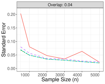
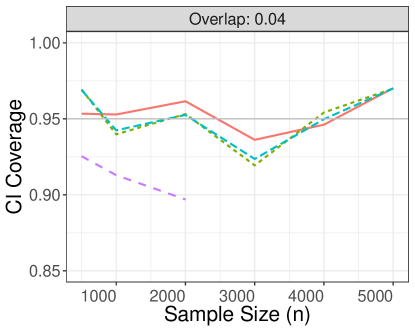
(a) Linearity and moderate overlap ($c_{0}\approx 0.04$)

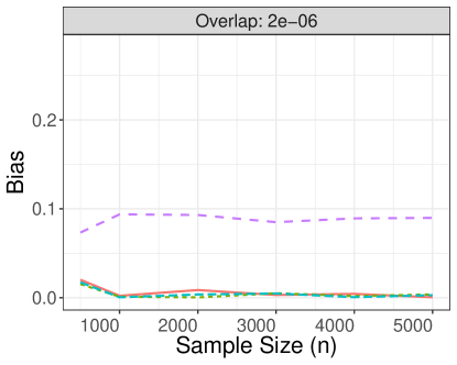
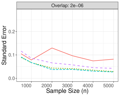
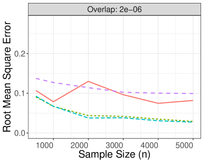
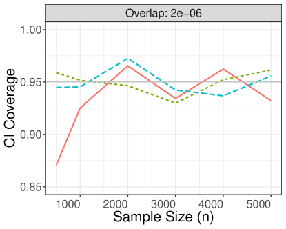
(b) Linearity and limited overlap ($c_{0}\approx 10^{-6}$)

Figure 1: Comparison of empirical bias, standard error and root mean squared error of estimator, and coverage of nominal 95% confidence interval for partially linear and plug-in HAL-ADMLEs, prespecified semiparametric estimator (assuming constant CATE), and nonparametric AIPW estimator, under sampling from a fixed distribution satisfying linearity and with varying degrees of treatment overlap. Coverage probabilities for intervals based on the prespecified semiparametric estimator were consistently poor, exceeding the y-axis range.

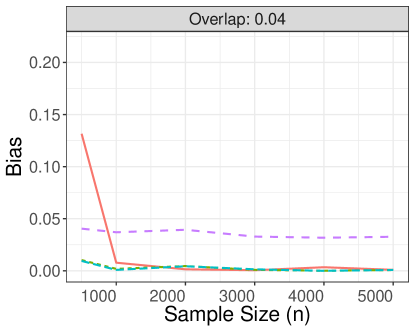
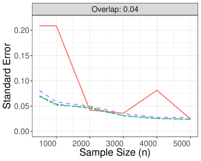
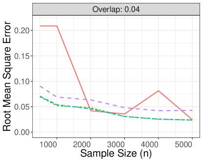
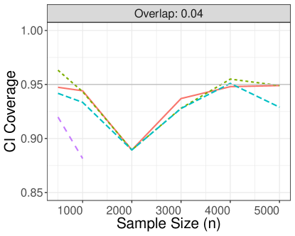
(a) Nonlinearity and moderate overlap ($c_{0}\approx 0.04$)

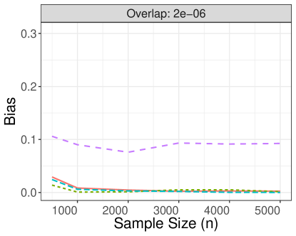
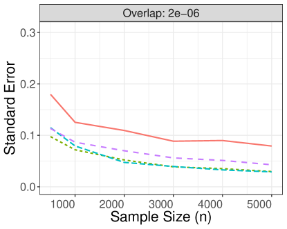
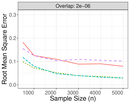
(b) Nonlinearity and limited overlap ($c_{0}\approx 10^{-6}$)

Figure 2: Comparison of empirical bias, standard error and root mean squared error of estimator, and coverage of nominal 95% confidence interval for partially linear and plug-in HAL-ADMLEs, prespecified semiparametric estimator (assuming constant CATE), and nonparametric AIPW estimator, under sampling from a fixed distribution not satisfying linearity and with varying degrees of treatment overlap. Coverage probabilities for intervals based on the prespecified semiparametric estimator were consistently poor, exceeding the y-axis range.

Based on our theory, in the case of a simple linear relationship that is sparse under the HAL basis, the plug-in ADMLE is expected to demonstrate greater efficiency than the partially linear ADMLE. In the nonlinear scenario, we anticipate comparable efficiency between the two estimators. Our experimental results align with these expectations, as we observe that the standard error of the plug-in ADMLE is generally smaller in the linear case with limited overlap. Moreover, in the nonlinear case, the two estimators appear to have the same large-sample variance. Although the plug-in ADMLE is generally more efficient than the partially linear ADMLE, it is important to note that it is typically irregular under a larger class of local alternatives. Additionally, the plug-in ADMLE lacks quasi double-robustness in the sense outlined in Condition E6, which limits its ability to take advantage of the smoothness properties of the propensity score.

6.2.2 Demonstrating irregularity: sampling under a least-favorable local alternative

In this experiment, we evaluate the performance of the estimators considered under a least-favorable local perturbation $P_{0,hn^{-1/2}}$ to $P_{0}$ for the ATE within a nonparametric statistical model. To achieve this, we introduce a local perturbation to the outcome regression components $\mu_{0}(0,\cdot)$ and $\tau$. Specifically, we define the control conditional mean corresponding to $P_{0,hn^{-1/2}}$ pointwise as $\mu_{n,0}(0,w):=\mu_{0}(0,w)-n^{-1/2}/\{1-\pi_{0}(w)\}$, and also define the CATE pointwise as $\Pi_{n}\tau_{0}(w):=1+n^{-1/2}/[\pi_{0}(w)\{1-\pi_{0}(w)\}]$, where $n$ represents the sample size in a given simulation. The remaining components of the data-generating distribution remain unchanged. It is important to note that, apart from the local perturbation, the prespecified semiparametric estimator based on the intercept CATE model is correctly specified. Moreover, the oracle submodel $\mathcal{M}_{0}$ corresponding to the unperturbed distribution $P_{0}$ is given by the partially linear intercept model. Therefore, we expect from Corollary 1 that the partially linear ADMLE is asymptotically equivalent under sampling from $P_{0,hn^{-1/2}}$ to the prespecified semiparametric estimator. The experimental results under linearity with moderate and limited treatment overlap are displayed in Figure 3, while results for other settings exhibit similar qualitative patterns and can be found in Appendix A.

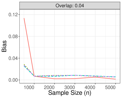
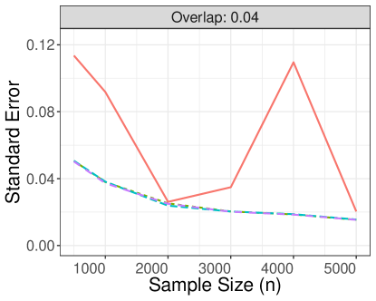
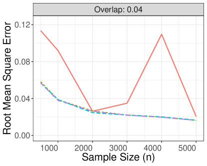
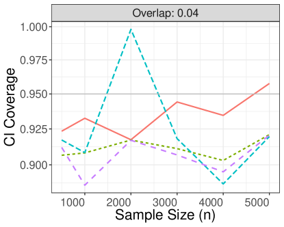
(a) Linearity and moderate overlap ($c_{0}\approx 0.04$)

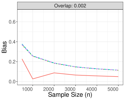
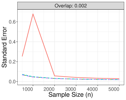
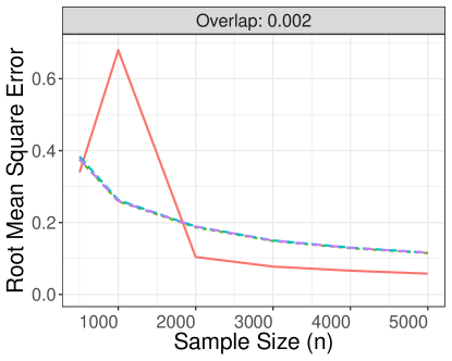
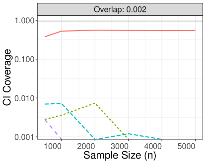
(b) Linearity and limited overlap ($c_{0}\approx 0.002$)

Figure 3: Comparison of empirical bias, standard error and root mean squared error of estimator, and coverage of nominal 95% confidence interval for partially linear and plug-in HAL-ADMLEs, prespecified semiparametric estimator (assuming constant CATE), and nonparametric AIPW estimator, under sampling from a least-favorable local perturbation of a distribution satisfying linearity in outcome regression and with varying degrees of treatment overlap. Coverage probabilities for intervals based on the prespecified semiparametric estimator were consistently poor, exceeding the y-axis range.

We find empirical support for the theoretical predictions implied by our results about the behavior of the estimators when sampling from a least-favorable local perturbation. Specifically, the prespecified semiparametric estimator and ADMLEs exhibit irregularity relative to the nonparametric model, leading to nonvanishing asymptotic bias. However, all estimators demonstrate $\sqrt{n}\,$–consistency as expected. However, consistent with Corollary 1, the prespecified semiparametric estimator based on the intercept CATE model appears to be asymptotically equivalent to the partially linear ADMLE. This suggests that there is no asymptotic loss in learning the oracle submodel from data compared to knowing it in advance, even under the least-favorable local alternative.

Notably, confidence intervals based on the AIPW estimator achieve 95% coverage under the least-favorable local perturbation due to its regularity, but at the cost of significantly increased variance. Moreover, the AIPW estimator performs worse in terms of mean squared error in the moderate overlap setting, with only marginal improvement in confidence interval coverage. We note that for overlap constant $c_{0}\approx 10^{-6}$ the AIPW estimator is biased and highly variable, likely due to the lack of identifiability of the ATE in the nonparametric model. In the linear case, we observe higher asymptotic bias in the plug-in ADMLE compared to the partially linear ADMLE, in line with expectations given that the former is regular under a smaller oracle submodel.

7.   Conclusion

Adaptive debiased machine learning provides a general approach for constructing asymptotically linear and superefficient estimators of pathwise differentiable parameters using data-driven model selection techniques. In this work, we showed that ADMLEs are regular and provide locally uniformly valid inference for an oracle projection-based parameter that agrees with the target parameter for distributions contained in the oracle statistical submodel. Our findings establish that, in a local asymptotic sense over a nonparametric model, there is no disadvantage in performing data-driven model selection compared to having prior knowledge of the oracle submodel. In addition, we demonstrated how to construct ADMLEs that exhibit, in a local asymptotic sense, comparable or better performance compared to any predefined estimator relying on parametric or semiparametric model assumptions, while also providing robustness against model misspecification. While we focused on the iid data setting, our results can be easily adapted to dependent data settings by applying suitable central limit theorems, e.g., as in van der Laan, (2014).

While our results indicate that data-driven model selection does not impact the asymptotic bias or variance of the ADMLE, it has the potential to cause finite-sample variance inflation, which can lead to suboptimal confidence interval coverage. To address this issue, sample-splitting could be used to reduce the dependence between the estimator and the working model. This technique involves dividing the available data into two halves, computing the working model and estimator separately on each half. To fully restore efficiency, this process could then be repeated by exchanging the roles of the data halves and taking the final ADMLE to be the average of the split-specific ADMLEs. Our theory can be readily applied to establish the asymptotic linearity and efficiency of this split-averaged ADMLE for the oracle target parameter. This approach can be extended to multi-fold splits using cross-fitting techniques (van der Laan and Rose, , 2011; Chernozhukov et al., 2018a, ). Alternatively, to address the additional finite sample variation introduced by data-driven model selection, bootstrap techniques (Efron and Tibshirani, , 1994; Cai and van der Laan, , 2019; Rinaldo et al., , 2019) or subsampling techniques (Guo and Shah, , 2023) could be considered for variance estimation.

Appendix A Supplementary experimental results

Sampling from true distribution

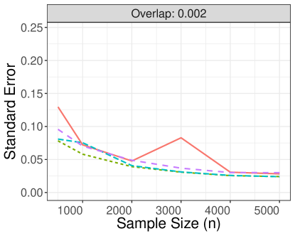
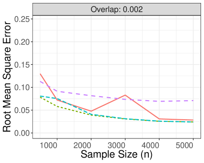
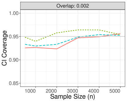
(a) Linear setting

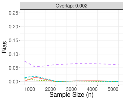
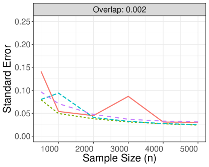
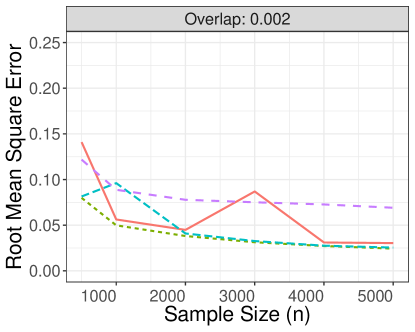
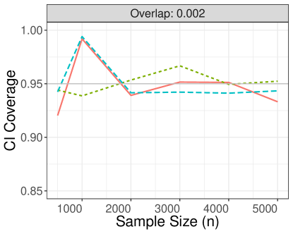
(b) Nonlinear setting

Figure 4: Comparison of empirical bias, standard error and root mean squared error of estimator, and coverage of nominal 95% confidence interval for partially linear and plug-in HAL-ADMLEs, prespecified semiparametric estimator (assuming constant CATE), and nonparametric AIPW estimator, under sampling from a fixed distribution satisfying linearity and with varying degrees of treatment overlap. Coverage probabilities for intervals based on the prespecified semiparametric estimator were consistently poor, exceeding the y-axis range.

Sampling from least-favorable local alternative

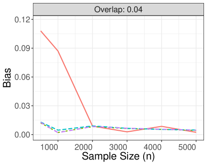
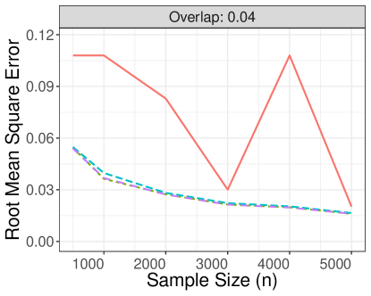
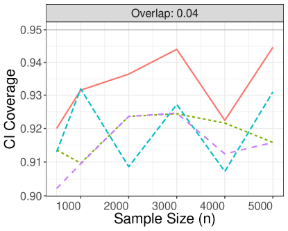
(a) Nonlinearity and moderate overlap ($c_{0}\approx 0.04$)

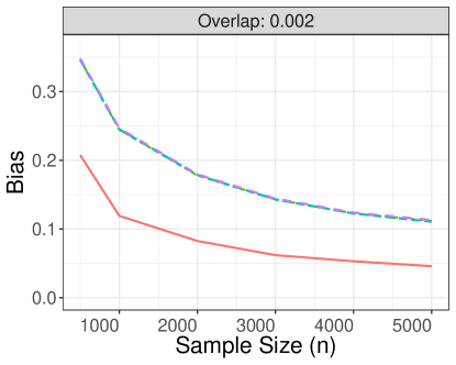
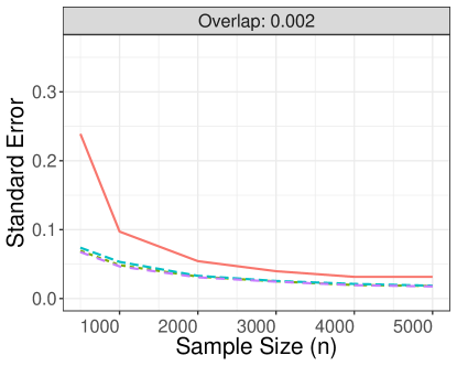
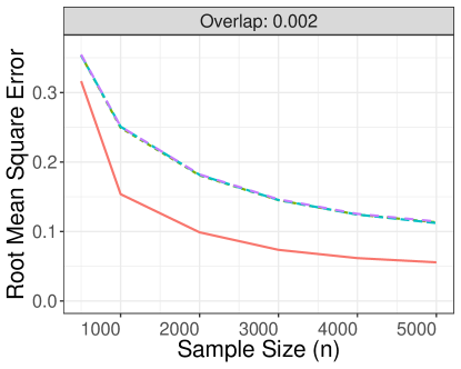
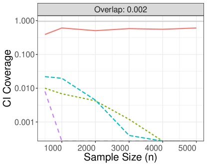
(b) Nonlinearity and limited overlap ($c_{0}\approx 0.002$)

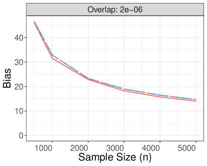
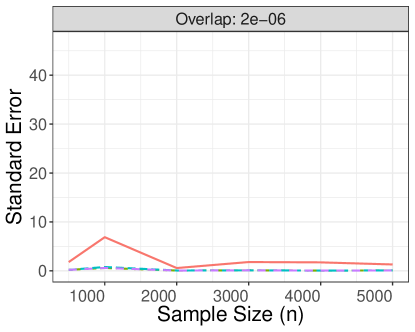
(c) Linearity and no overlap ($c_{0}\approx 10^{-6}$)

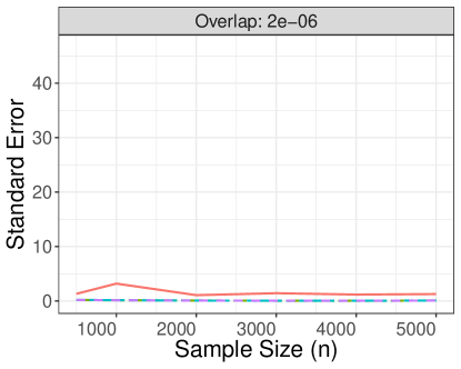
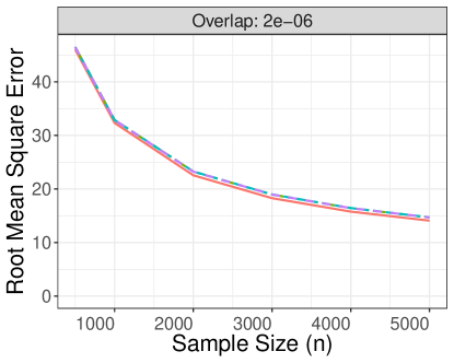
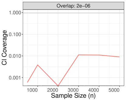
(d) Nonlinearity and no overlap ($c_{0}\approx 10^{-6}$)

Figure 5: Comparison of empirical bias, standard error and root mean squared error of estimator, and coverage of nominal 95% confidence interval for partially linear and plug-in HAL-ADMLEs, prespecified semiparametric estimator (assuming constant CATE), and nonparametric AIPW estimator, under sampling from a least-favorable local perturbation of a distribution satisfying linearity in outcome regression and with varying degrees of treatment overlap.

Appendix B Proofs of theoretical results

Proof of Theorem 1.

Let $P\in\mathcal{M}_{np}$ be arbitrary. By A3 and A4, a minimizing solution $Q_{P}\in\operatorname*{argmin}_{Q\in\mathcal{M}_{0}}P\ell(\cdot,Q)$ satisfies

$$\frac{d}{dt}P\ell(\cdot,Q_{t})\big{|}_{t=0}=P\left\{\frac{d}{dt}\ell(\cdot,Q_{t})\big{|}_{t=0}\right\}=0,$$

for all regular paths $(Q_{t}:t\in(-\varepsilon,\varepsilon))\subseteq\mathcal{M}_{0}$ with $Q_{t}=Q_{P}$ at $t=0$.

For some $\delta>0$, let $(P_{t}:t\in(-\delta,\delta))\subseteq\mathcal{M}_{np}$ be a regular path through $P$ such that $dP_{t}=(1+ts)dP$ for a bounded score $s\in L^{2}_{0}(P)$ orthogonal to the loss-based tangent space $\mathcal{S}_{\mathcal{M}_{0}}(P)$. Since ${\cal M}_{np}$ is a convex nonparametric model and the score $s$ is bounded, such a path necessarily exists for sufficiently small $\delta>0$. By Condition A4, for all regular paths $(Q_{u}:u\in(-\varepsilon,\varepsilon))\subseteq\mathcal{M}_{0}$ through $Q_{P}$ at $u=0$, we have

$$P_{t}\left\{\frac{d}{du}\ell(\cdot,Q_{u})\big{|}_{u=0}\right\} =\int\left\{\frac{d}{du}\ell(o,Q_{u})\big{|}_{u=0}\right\}\{1+ts(o)\}P(do)$$

$$=\int\left\{\frac{d}{du}\ell(o,Q_{u})\big{|}_{u=0}\right\}P(do)+t\int\left\{\frac{d}{du}\ell(o,Q_{u})\big{|}_{u=0}\right\}s(o)P(do)\ .$$

The first term on the right-hand side is $0$ since $Q_{P}$ is a minimizer of $Q\mapsto P\ell(\cdot,Q)$ over $Q\in\mathcal{M}_{0}$. The second term on the right-hand side is also $0$ since $s$ is centered under $P$ and, by construction, orthogonal to $\frac{d}{du}\ell(\cdot,Q_{u})\big{|}_{u=0}\in\mathcal{S}_{\mathcal{M}_{0}}(P)$. It follows that $P_{t}\left\{\frac{d}{du}\ell(\cdot,Q_{u})\big{|}_{u=0}\right\}=0$ for all such paths $(Q_{u}:u\in(-\varepsilon,\varepsilon))\subseteq\mathcal{M}_{0}$ and $t$ sufficiently small. By Condition A4, this can only occur if $Q_{P}\in\operatorname*{argmin}_{Q\in\mathcal{M}_{0}}P_{t}\ell(\cdot,Q)$ for all $t$ sufficiently small.

By Condition A2, $\Psi_{0}=\Psi\circ\Pi_{0}$ is pathwise differentiable at $P_{0}$; thus, its efficient influence function $D_{0,P_{0}}$ exists and is contained in $L^{2}_{0}(P_{0})$. For some sufficiently small $\delta>0$, let $(P_{t}:t\in(-\delta,\delta))\subseteq\mathcal{M}_{np}$ be a regular path through $P_{0}$ such that $dP_{t}=(1+ts)dP_{0}$ with score $s\in L^{2}_{0}(P_{0})$ orthogonal to the loss-based tangent space $\mathcal{S}_{\mathcal{M}_{0}}(P_{0})$. Then, by the above and A1, our chosen path $(P_{t}:t\in(-\varepsilon,\varepsilon)$ is such that $\Psi_{0}(P_{t})=\Psi(\Pi_{0}P_{t})=\Psi(Q_{P_{0}})$ for all $t$ sufficiently small. Thus, upon differentiation, we find that

$$0=\frac{d}{dt}\Psi_{0}(P_{t})\big{|}_{t=0}=\langle D_{0,P_{0}},s\rangle_{L^{2}(P_{0})}.$$

Thus, $D_{0,P_{0}}$ is necessarily orthogonal to the score $s$ in $L^{2}_{0}(P_{0})$. However, $s$ was an arbitrary bounded score taken to be orthogonal to the loss-based tangent space $\mathcal{S}_{\mathcal{M}_{0}}(P_{0})$. Since $\mathcal{S}_{\mathcal{M}_{0}}(P)$ is a closed linear space and bounded scores are dense in $L^{2}_{0}(P_{0})$, we must have that $D_{0,P_{0}}\in\mathcal{S}_{\mathcal{M}_{0}}(P)$. The result then follows.∎

Proof of Theorem 3.

By B1–B3, we have

$$\widehat{\psi}_{n}-\Psi_{n}(P_{0})\ =\ (P_{n}-P_{0})D_{n,P_{0}}+o_{p}(n^{-1/2})$$

$$=\ (P_{n}-P_{0})D_{0,P_{0}}+(P_{n}-P_{0})(D_{n,P_{0}}-D_{0,P_{0}})+o_{p}(n^{-1/2})$$

$$=\ (P_{n}-P_{0})D_{0,P_{0}}+o_{p}(n^{-1/2})\ ,$$

where the final equality uses, by B3, that $(P_{n}-P_{0})(D_{n,P_{0}}-D_{0,P_{0}})=o_{p}(n^{-1/2})$. The result now follows. We note that B2, while not used in this proof, is typically required to establish B3.∎

Proof of Lemma 1.

Under B2enumiB2enumia and by Theorem 1, $D_{n,P_{n,0}}\in T_{\mathcal{M}_{n}}(P_{n,0})$ and $D_{0,P_{n,0}}\in T_{\mathcal{M}_{0}}(P_{n,0})$ are the $P_{n,0}$–efficient influence functions of $\Psi$ relative to the models $\mathcal{M}_{n}$ and $\mathcal{M}_{0}$, respectively. Under B2enumiB2enumid, we have $T_{\mathcal{M}_{n}}(P_{n,0})\subseteq T_{\mathcal{M}_{0}}(P_{n,0})$, with probability tending to one. On this event, we claim that $D_{n,P_{n,0}}=\bar{D}_{0,P_{n,0}}:=\bar{\Pi}_{n}D_{0,P_{n,0}}$, where $\bar{\Pi}_{n}:T_{\mathcal{M}_{0}}(P_{n,0})\rightarrow T_{\mathcal{M}_{n}}(P_{n,0})$ is the $L^{2}(P_{n,0})$–projection onto $T_{\mathcal{M}_{0}}(P_{n,0})$. First, on this event, since $D_{0,P_{n,0}}$ is a gradient for $d\Psi(P_{n,0})$ relative to $T_{\mathcal{M}_{0}}(P_{n,0})$, we have that $\bar{D}_{0,P_{n,0}}$ is a gradient for $d\Psi(P_{n,0})$ relative to $T_{\mathcal{M}_{n}}(P_{n,0})$. Since $\Psi=\Psi_{n}$ on $\mathcal{M}_{n}$, this implies, for all $s\in T_{\mathcal{M}_{n}}(P_{n,0})$, that $d\Psi_{n}(P_{n,0})[s]=\langle s,\bar{D}_{0,P_{n,0}}\rangle_{P_{n,0}}$. However, we also know that $d\Psi_{n}(P_{n,0})[s]=\langle s,D_{n,P_{n,0}}\rangle_{P_{n,0}}$, and thus, for all $s\in T_{\mathcal{M}_{n}}(P_{n,0})$,

$$\langle s,\bar{D}_{0,P_{n,0}}-D_{n,P_{n,0}}\rangle_{P_{n,0}}=0\ .$$

Since both $\bar{D}_{0,P_{n,0}}$ and $D_{n,P_{n,0}}$ are elements of $T_{\mathcal{M}_{n}}(P_{n,0})$, we must have that $D_{n,P_{n,0}}=\bar{D}_{0,P_{n,0}}$ on this event. Finally, by the triangle inequality, B2enumiB2enumib and B2enumiB2enumic, we have that

$$\norm{D_{n,P_{0}}-D_{0,P_{0}}}_{P_{0}}\ \leq\ \norm{D_{n,P_{n,0}}-D_{n,P_{0}}}_{P_{0}}+\norm{D_{0,P_{n,0}}-D_{0,P_{0}}}_{P_{0}}+\norm{D_{0,P_{n,0}}-\bar{D}_{0,P_{n,0}}}_{P_{0}}+o_{p}(1)$$

$$=\ o_{p}(1)\ ,$$

where we used that $T_{\mathcal{M}_{n}}(P_{n,0})\subseteq T_{\mathcal{M}_{0}}(P_{n,0})$, and so, $D_{n,P_{n,0}}=\bar{D}_{0,P_{n,0}}$ occurs with probability tending to one. The result then follows. ∎

Proof of Lemma 2.

By Condition A2, the data-dependent efficient influence function $D_{0,P_{n,0}}\in T_{\mathcal{M}_{0}}(P_{n,0})$ at $P_{n,0}=\Pi_{n}P_{0}$ exists. Using that $\Psi(P_{n,0})-\Psi(\Pi_{0}P_{n,0})=o_{p}(n^{-1/2})$, we have the exact expansion

$$\Psi_{n}(P_{0})-\Psi_{0}(P_{0})\ =\ \Psi(P_{n,0})-\Psi(\Pi_{0}P_{n,0})+\Psi(\Pi_{0}P_{n,0})-\Psi_{0}(P_{0})$$

$$=\ o_{p}(n^{-1/2})+\Psi_{0}(P_{n,0})-\Psi_{0}(P_{0})$$

$$=\ -P_{0}D_{0,P_{n,0}}+R_{n,0}+o_{p}(n^{-1/2})$$

$$=\ (P_{n,0}-P_{0})D_{0,P_{n,0}}+R_{n,0}+o_{p}(n^{-1/2})\ ,$$ (4)

where $R_{n,0}:=\Psi_{0}(P_{n,0})-\Psi_{0}(P_{0})+P_{0}D_{0,P_{n,0}}$ is the exact second-order remainder. Now, by A4, we have that the minimizer $P_{n,0}=\Pi_{n}P_{0}$ satisfies

$$P_{0}\left\{\frac{d}{dt}\ell(\cdot,Q_{t})\big{|}_{t=0}\right\}=0$$ (5)

for all regular paths $(Q_{t}:t\in(-\delta,\delta))\subseteq\mathcal{M}_{n}$ such that $Q_{t}=\Pi_{n}P_{0}$ at $t=0$. By definition, we have that $\bar{D}_{0,P_{n,0}}$ is contained in the loss-based tangent space $\mathcal{S}_{\mathcal{M}_{n}}(P_{n,0})\subseteq L^{2}_{0}(P_{n,0})$. Thus, there exists some regular path $(Q_{t}:t\in(-\delta,\delta))\subseteq\mathcal{M}_{n}$ such that $Q_{t}=P_{n,0}$ at $t=0$ and $\frac{d}{dt}\ell(\cdot,Q_{t})\big{|}_{t=0}=\bar{D}_{0,P_{n,0}}$. Moreover, by Equation (5), we must have that

$$P_{0}(\bar{D}_{0,P_{n,0}})=P_{0}\left\{\frac{d}{dt}\ell(\cdot,Q_{t})\big{|}_{t=0}\right\}=0\ .$$

Since $\bar{D}_{0,P_{n,0}}\in L^{2}_{0}(P_{n,0})$ is centered under $P_{n,0}$, we also have $(P_{n,0}-P_{0})\bar{D}_{0,P_{n,0}}=0$. Combining this with Equation (4), we obtain the expansion

$$\Psi_{n}(P_{0})-\Psi_{0}(P_{0})=(P_{n,0}-P_{0})(D_{0,P_{n,0}}-\bar{D}_{0,P_{n,0}})+R_{n,0}+o_{p}(n^{-1/2})\ ,$$

as desired.∎

Proof of Theorem 5.

Under C1, the proof of Lemma 2 establishes the bound

$$\Psi_{n}(P_{0})-\Psi_{0}(P_{0})=(P_{n,0}-P_{0})(D_{0,P_{n,0}}-\bar{D}_{0,P_{n,0}})+R_{n,0}+o_{p}(n^{-1/2})\ .$$

Combining this with Theorem 3, we obtain the expansion

$$\widehat{\psi}_{n}-\Psi_{0}(P_{0})\ =\ (P_{n}-P_{0})D_{0,P_{0}}+o_{p}(n^{-1/2})$$

$$\qquad+(P_{n,0}-P_{0})(D_{0,P_{n,0}}-\bar{D}_{0,P_{n,0}})+R_{n,0}+o_{p}(n^{-1/2})\ .$$

By C2, we have that $(P_{n,0}-P_{0})(D_{0,P_{n,0}}-\bar{D}_{0,P_{n,0}})+R_{n,0}=o_{p}(n^{-1/2})$, and so, $\widehat{\psi}_{n}-\Psi_{0}(P_{0})=(P_{n}-P_{0})D_{0,P_{0}}+o_{p}(n^{-1/2})$ as desired. It follows that $\widehat{\psi}_{n}$ is asymptotically linear at $P_{0}$ for $\Psi_{0}:\mathcal{M}_{np}\rightarrow\mathbb{R}$ with influence function being the efficient influence function of $\Psi_{0}$ at $P_{0}$. Hence, $\widehat{\psi}_{n}$ is $P_{0}$–efficient for $\Psi_{0}$ relative to $\mathcal{M}_{np}$ (Bickel et al., , 1993). Moreover, since $\widehat{\psi}_{n}$ is efficient, it is necessarily regular for $\Psi_{0}$ relative to $\mathcal{M}_{np}$ (van der Vaart, , 2000). The limiting distribution result follows immediately from the central limit theorem and Slutsky’s lemma.∎

Proof of Theorem 6.

By Theorem 5 and that $\Psi_{0}(P_{0})=\Psi(P_{0})$, the ADMLE $\widehat{\psi}_{n}$ is asymptotically linear for $\Psi$ at $P_{0}$ with influence function being the efficient influence function of $\Psi_{0}$. Since $\Psi_{0}(P)=\Psi(P)$ for all $P\in\mathcal{M}_{0}$, regularity of the ADMLE for $\Psi_{0}$ over $\mathcal{M}_{np}$ implies that the ADMLE is regular for $\Psi$ over the oracle submodel $\mathcal{M}_{0}$. Under the loss-based tangent space conditions, we have by Theorem 1 that $D_{0,P_{0}}$ is the efficient influence function of $\Psi$ relative to $\mathcal{M}_{0}$. Thus, the ADMLE is asymptotically linear with influence function equal to the efficient influence function of $\Psi$ relative to $\mathcal{M}_{0}$. It follows that the ADMLE is asymptotically efficient (van der Vaart, , 2000).∎

Proof of Theorem 7.

We assumed that $\Psi$ is pathwise differentiable at $P_{0}$ relative to $\mathcal{M}$ with efficient influence function $D_{\mathcal{M},P_{0}}$. Using that $\Psi_{0}(P_{0})=\Psi(P_{0})$, we first observe that

$$\Psi_{0}(P_{0,hn^{-1/2}})-\Psi(P_{0,hn^{-1/2}})\ =\ \Psi_{0}(P_{0,hn^{-1/2}})-\Psi_{0}(P_{0})+\Psi(P_{0})-\Psi(P_{0,hn^{-1/2}})$$

$$=\ hn^{-1/2}\{d\Psi_{0}(P_{0})(S)-d\Psi(P_{0})(S)\}+o(n^{-1/2})$$

$$=\ hn^{-1/2}\langle S,D_{0,P_{0}}-D_{\mathcal{M},P_{0}}\rangle_{P_{0}}+o(n^{-1/2})\ ,$$

where the final two equalities use pathwise differentiability of $\Psi:\mathcal{M}\rightarrow\mathbb{R}$ and $\Psi_{0}:\mathcal{M}_{np}\rightarrow\mathbb{R}$. Hence, we find that

$$\sqrt{n}\left\{\widehat{\psi}_{n}-\Psi(P_{0,hn^{-1/2}})\right\}\ =\ \sqrt{n}\left\{\widehat{\psi}_{n}-\Psi_{0}(P_{0,hn^{-1/2}})\right\}+\sqrt{n}\left\{\Psi_{0}(P_{0,hn^{-1/2}})-\Psi(P_{0,hn^{-1/2}})\right\}$$

$$=\ \sqrt{n}\,(P_{n}-P_{0})D_{0,P_{0}}+h\langle S,D_{0,P_{0}}-D_{\mathcal{M},P_{0}}\rangle_{P_{0}}+o(1)\ .$$

The result then follows from Slutsky’s theorem.∎

Appendix C Theory and proofs for plug-in ADMLE of ATE

In this section, we provide the efficient influence function for the oracle ATE parameter provided by (3). Moreover, we analyze the estimation and oracle bias of the plug-in ADMLE for the ATE considered in Example 2 and establish its efficiency for the oracle parameter.

Recall the setup of Section 2.3. Let $\alpha_{0}:=\operatorname*{argmin}_{\alpha\in\Theta_{0}}E_{0}\left[\alpha(A,W)^{2}-2\{\alpha(1,W)-\alpha(0,W)\}\right]$ be the Riesz representer of the ATE functional with respect to $\Theta_{0}$. Let $\Theta_{n}$ be a data-dependent working linear regression model of finite dimension and consider the plug-in ADMLE of the ATE

$$\widehat{\psi}_{n}:=\frac{1}{n}\sum_{i=1}^{n}\left\{\mu_{n}(1,W_{i})-\mu_{n}(0,W_{i})\right\}$$

with $\mu_{n}:=\operatorname*{argmin}_{\theta\in\Theta_{n}}\sum_{i=1}^{n}\{Y_{i}-\mu_{n}(A_{,}W_{i})\}^{2}$.

The following lemma is a direct corollary of the efficient influence function derivations provided in the proofs of Theorem 4.1 and 4.2 of Chernozhukov et al., 2018b — see also Chernozhukov et al., 2018c for additional details.

Lemma 3.

Let $\Theta\subseteq L^{2}(P_{A,W})$ be a closed linear space and $\Pi_{P}\mu_{P}:=\operatorname*{argmin}_{\theta\in\Theta}\|\mu_{P}-\theta\|_{L^{2}(P)}$ denote the projection of $\mu_{P}$ onto $\Theta$. Suppose that $\theta\mapsto E_{P}\left\{\theta(1,W)-\theta(0,W)\right\}$ is a bounded linear functional over $\Theta$. Then, the projection parameter $\Psi_{\Theta}:P\mapsto E_{P}\left\{\Pi_{P}\mu_{P}(1,W)-\Pi_{P}\mu_{P}(0,W)\right\}$ is pathwise differentiable at $P$ under a locally nonparametric statistical model with efficient influence function given almost everywhere by

$$D_{P}:o\mapsto\alpha_{P}(a,w)\left\{y-\Pi_{P}\mu_{P}(a,w)\right\}+\Pi_{P}\mu_{P}(1,w)-\Pi_{P}\mu_{P}(0,w)-\Psi(P)\ ,$$

where $\alpha_{P}:=\operatorname*{argmin}_{\alpha\in\Theta}E_{P}\left[\alpha(A,W)^{2}-2\{\alpha(1,W)-\alpha(0,W)\}\right]$ is the Riesz representer.

The following lemmas provide bounds for the estimation bias $\widehat{\psi}_{n}-\Psi_{n}(P_{0})$ and oracle bias $\Psi_{n}(P_{0})-\Psi_{0}(P_{0})$.

Lemma 4 (Oracle bias is second-order).

On the event $\{\Pi_{n}\mu_{0}\in\Theta_{0}\}$, which necessarily occurs if $\Theta_{n}\subseteq\Theta_{0}$, we have that

$$\Psi_{n}(P_{0})-\Psi_{0}(P_{0})=E_{0}\left[\left\{\alpha_{0}(A,W)-\Pi_{n}\alpha_{0}(A,W)\right\}\{\Pi_{n}\mu_{0}(A,W)-\mu_{0}(A,W)\}\right].$$

Proof.

We have that $\Psi_{n}(P_{0})=E_{0}\left\{\Pi_{n}\mu_{0}(1,W)-\Pi_{n}\mu_{0}(0,W)\right\}$, where $\Pi_{n}\mu_{0}$ denotes the projection $\operatorname*{argmin}_{\theta\in\Theta_{n}}E_{0}\left\{\mu_{0}(A,W)-\theta(A,W)\right\}^{2}$. Let $\alpha_{0}\in\Theta_{0}$ be the Riesz representer of the ATE functional with respect to $\Theta_{0}$, so that $E_{0}\left\{\mu(1,W)-\mu(0,W)\right\}=E_{0}\left\{\alpha_{0}(A,W)\mu(A,W)\right\}$ for all $\mu\in\Theta_{0}$. Then, since $\Pi_{n}\mu_{0},\mu_{0}\in\Theta_{0}$, we have that

$$\Psi_{n}(P_{0})-\Psi_{0}(P_{0})=E_{0}\left[\alpha_{0}(A,W)\{\Pi_{n}\mu_{0}(A,W)-\mu_{0}(A,W)\}\right].$$

Moreover, we have that $E_{0}\left[\Pi_{n}\alpha_{0}(A,W)\{\Pi_{n}\mu_{0}(A,W)-\mu_{0}(A,W)\}\right]=0$ since the orthogonal projection $\Pi_{n}\mu_{0}$ has the property that $\Pi_{n}\mu_{0}-\mu_{0}$ is orthogonal to $\Theta_{n}$ in $L^{2}(P_{0})$. Hence, the previous display gives that $\Psi_{n}(P_{0})-\Psi_{0}(P_{0})=E_{0}\left[\left\{\alpha_{0}(A,W)-\Pi_{n}\alpha_{0}(A,W)\right\}\{\Pi_{n}\mu_{0}(A,W)-\mu_{0}(A,W)\}\right]$.∎

Lemma 5.

Suppose $\Theta_{n}\subseteq\Theta_{0}$ with probability tending to one. Then, with $D_{n,\widehat{P}_{n}}$ denoting the map $o\mapsto\Pi_{n}\alpha_{0}(a,w)\left\{y-\mu_{n}(a,w)\right\}+\mu_{n}(1,w)-\mu_{n}(0,w)$, we have that $\widehat{\psi}_{n}-\Psi_{n}(P_{0})=(P_{n}-P_{0})D_{n,\widehat{P}_{n}}$.

Proof.

The first-order equations characterizing the empirical risk minimizer $\mu_{n}$ imply that

$$\frac{1}{n}\sum_{i=1}^{n}\Pi_{n}\alpha_{0}(A_{i},W_{i})\left\{Y_{i}-\mu_{n}(A_{i},W_{i})\right\}=0\ .$$

Since $\Theta_{n}\subseteq\Theta_{0}$, we have that

$$\widehat{\psi}_{n}=\frac{1}{n}\sum_{i=1}^{n}\left[\mu_{n}(1,W_{i})-\mu_{n}(0,W_{i})+\Pi_{n}\alpha_{0}(A_{i},W_{i})\left\{Y_{i}-\mu_{n}(A_{i},W_{i})\right\}\right]=P_{n}D_{n,\widehat{P}_{n}}\ .$$

Next, since $\Theta_{n}\subseteq\Theta_{0}$, we also have that $\Pi_{n}\alpha_{0}$ is the Riesz representer of the ATE linear functional relative to $\Theta_{n}$ (Chernozhukov et al., 2018b, ). Hence, we have that $E_{0}\left\{\mu_{n}(1,W)-\mu_{n}(0,W)\right\}=E_{0}\left\{\Pi_{n}\alpha_{0}(A,W)\mu_{n}(A,W)\right\}$, and consequently, that

$$E_{0}\left[\mu_{n}(1,W)-\mu_{n}(0,W)+\Pi_{n}\alpha_{0}(A,W)\left\{Y-\mu_{n}(A,W)\right\}\right]$$

$$=\ E_{0}\left[\Pi_{n}\alpha_{0}\mu_{n}+\Pi_{n}\alpha_{0}(A,W)\left\{Y-\mu_{n}(A,W)\right\}\right]$$

$$=\ E_{0}\left\{\Pi_{n}\alpha_{0}(A,W)Y\right\}\ =\ E_{0}\left\{\Pi_{n}\alpha_{0}(A,W)\mu_{0}(A,W)\right\}\ =\ \Psi_{n}(P_{0})\ .$$

Combining the previous two displays, it follows that $\widehat{\psi}_{n}-\Psi_{n}(P_{0})=(P_{n}-P_{0})D_{n,\widehat{P}_{n}}$.∎

Finally, we are ready to give our main theorem on the asymptotic behavior of the plug-in ADMLE of the ATE.

1. Donsker condition: $\Pi_{n}\alpha_{0}$ and $\mu_{n}$ are uniformly bounded and fall in a fixed Donsker class with probability tending to one.

2. Nested working model: $\liminf_{n\rightarrow\infty}P({\Theta}_{n}\subseteq{\Theta}_{0})=1$.

3. Consistency: $\norm{\Pi_{n}\alpha_{0}-\alpha_{0}}_{P_{0}}=o_{p}(1)$ and $\max_{a\in\{0,1\}}\norm{\mu_{n}(a,\cdot)-\mu_{0}(a,\cdot)}_{P_{0}}=o_{p}(1)$.

4. Negligible oracle bias: $\norm{\Pi_{n}\alpha_{0}-\alpha_{0}}_{P_{0}}\norm{\Pi_{n}\mu_{0}-\mu_{0}}_{P_{0}}=o_{p}(n^{-1/2})$.

Theorem 9.

Under S1–S4, the plug-in ADMLE $\widehat{\psi}_{n}$ is regular, asymptotically linear, and asymptotically efficient for $\Psi_{0}$ with $\widehat{\psi}_{n}-\Psi_{0}(P_{0})=(P_{n}-P_{0})D_{0,P_{0}}+o_{p}(n^{-1/2})$, where $D_{0,P_{0}}$ is the efficient influence function of $\Psi_{0}:\mathcal{M}_{np}\rightarrow\mathbb{R}$.

Proof.

Applying S2, Lemma 4, and Lemma 5, we find that

$$\widehat{\psi}_{n}-\Psi_{0}(P_{0})=(P_{n}-P_{0})D_{n,\widehat{P}_{n}}+E_{0}\left[\left\{\alpha_{0}(A,W)-\Pi_{n}\alpha_{0}(A,W)\right\}\{\Pi_{n}\mu_{0}(A,W)-\mu_{0}(A,W)\}\right].$$

By the Cauchy-Schwarz inequality and S4, we have that

$$E_{0}\left[\left\{\alpha_{0}(A,W)-\Pi_{n}\alpha_{0}(A,W)\right\}\{\Pi_{n}\mu_{0}(A,W)-\mu_{0}(A,W)\}\right]$$

$$\leq\ \norm{\Pi_{n}\alpha_{0}-\alpha_{0}}_{P_{0}}\norm{\Pi_{n}\mu_{0}-\mu_{0}}_{P_{0}}\ =\ o_{p}(n^{-1/2})\ .$$

Additionally, since $\Pi_{n}\alpha_{0}$ and $\mu_{n}$ are bounded in view of S1, we have that

$$\|D_{n,\widehat{P}_{n}}-D_{0,P_{0}}\|_{P_{0}}\ \lessapprox\ \max_{a\in\{0,1\}}\|\mu_{n}(a,\cdot)-\mu_{0}(a,\cdot)\|_{P_{0}}+\|\Pi_{n}\alpha_{0}-\alpha_{0}\|_{P_{0}}\ ,$$

which is $o_{P}(1)$ by S3. Finally, since $D_{n,\widehat{P}_{n}}$ is a Lipschitz transformation of $\mu_{n}$ and $\Pi_{n}\alpha_{0}$, we have by S1 that $D_{n,\widehat{P}_{n}}$ falls with probability tending to one in a Donsker function class (van der Vaart and Wellner, , 1996). Therefore, by stochastic asymptotic equicontinuity of empirical processes on Donsker classes, $\|D_{n,\widehat{P}_{n}}-D_{0,P_{0}}\|_{P_{0}}=o_{P}(1)$ implies that

$$(P_{n}-P_{0})D_{n,\widehat{P}_{n}}=(P_{n}-P_{0})D_{0,P_{0}}+o_{p}(n^{-1/2})\ .$$

Consequently, we have that $\widehat{\psi}_{n}-\Psi_{0}(P_{0})=(P_{n}-P_{0})D_{0,P_{0}}+o_{p}(n^{-1/2})$, as desired.∎

Appendix D Proofs for partially linear ADMLE of ATE

Proof of Theorem 2.

Let $\Theta_{0}:=\{(a,w)\mapsto m(w)+a\tau(w):m\in L^{2}(P_{0}),\tau\in\mathcal{T}_{0}\}$ be the corresponding oracle model for the outcome regression. By Lemma 3, the efficient influence function $D_{0,P}$ for $\Psi_{0}$ at $P$ under the prespecified statistical model $\mathcal{M}$ is given by $o\mapsto\Pi_{0}\tau_{P}(w)-E_{0}\{\Pi_{0}\tau_{P}(W)\}+\alpha_{P}(w)\{a-\pi_{P}(w)\}\{y-\mu_{P}(w)\}$, where $\alpha_{P}:=\operatorname*{argmin}_{\alpha\in\Theta_{0}}E_{P}\left[\alpha(A,W)^{2}-2\{\alpha(1,W)-\alpha(0,W)\}\right]$ is the Riesz representer of the linear functional $\mu\mapsto E_{P}\{\mu(1,W)-\mu(0,W)\}$ (Chernozhukov et al., 2018b, ; Chernozhukov et al., 2018c, ). We claim that $\alpha_{P}(A,W)=\gamma_{P}(W)\{A-\pi_{P}(W)\}$ $P$–almost surely. To see this, we observe that $\operatorname*{argmin}_{\alpha\in\Theta_{0}}E_{P}\left[\alpha(A,W)^{2}-2\{\alpha(1,W)-\alpha(0,W)\}\right]$ coincides with

$$\operatorname*{argmin}_{m\in L_{2}(P_{0}),\gamma\in\mathcal{T}_{0}}E_{P}\left[\{m(W)+A\gamma(W)\}^{2}-2\gamma(W)\right].$$ (6)

Next, we expand the objective function in (6) as

$$(m,\gamma)\mapsto E_{P}\left\{m(W)^{2}-2\pi_{P}(W)m(W)\gamma(W)+A^{2}\gamma(W)-2\gamma(W)\right\},$$

and observe that $m$ and $\gamma$ are able to vary freely in the minimization problem. Holding $\gamma$ fixed, we find that the above is minimized by $m_{P,\gamma}:w\mapsto-\pi_{P}(w)\gamma(w)$. With the choice $m=m_{P,\gamma}$, we obtain the profiled objective function $\gamma\mapsto E_{P}\left[\{A-\pi_{P}(W)\}^{2}\gamma(W)^{2}-2\gamma(W)\right]$, which is exactly minimized over $\gamma\in\mathcal{T}_{0}$ by $\gamma_{P}$. Thus, plugging in these optimizers, we conclude that $\alpha_{P}(a,w)=\{a-\pi_{P}(w)\}\gamma_{P}(w)$. Plugging this expression for $\alpha_{P}$ in $D_{0,P}$, we obtain the efficient influence function given in the theorem.∎

Proof of Theorem 4.

Due to Condition E3, we can assume, without loss of generality, that the event $\mathcal{T}_{n}\subseteq\mathcal{T}_{0}$ occurs. All our results remain valid since any convergence results derived conditionally on this event must also hold unconditionally, as the event occurs with a probability approaching one. In such case, we have that

$$\Pi_{n}\gamma_{0}\ := \ \ \operatorname*{argmin}_{\gamma\in\mathcal{T}_{n}}E_{0}\left[\{A-\pi_{0}(W)\}^{2}\gamma(W)^{2}-2\gamma(W)\right]$$

$$= \ \ \operatorname*{argmin}_{\gamma\in\mathcal{T}_{n}}E_{0}\left(\{A-\pi_{0}(W)\}^{2}\left[\gamma(W)-\{A-\pi_{0}(W)\}^{-2}\right]\right).$$

It follows that $\Pi_{n}\gamma_{0}$ is the overlap-weighted projection of $(a,w)\mapsto\{a-\pi_{0}(w)\}^{-2}$ onto $\mathcal{T}_{n}$. Since $\mathcal{T}_{n}\subseteq\mathcal{T}_{0}$, we also have that

$$\Pi_{n}\gamma_{0}:=\operatorname*{argmin}_{\gamma\in\mathcal{T}_{n}}E_{0}\left[(A-\pi_{0}(W))^{2}\left\{\gamma(W)-\gamma_{0}(W)\right\}\right],$$

where we note that $\Pi_{n}\gamma_{0}$ appears in the efficient influence function $D_{n,P_{0}}$ of $\Psi_{n}$ as indicated in Theorem 2.

Let $o\mapsto\widehat{D}_{n,0}(o):=\tau_{n}(w)-P_{n}\tau_{n}+\Pi_{n}\gamma_{0}(w)\{a-\pi_{n}(w)\}\{y-\mu_{n}(a,w)\}$ be an estimator of the efficient influence function $D_{0,P_{0}}$ of $\Psi_{0}$ provided in Theorem 2. By the first-order conditions characterizing the minimizer $\tau_{n}$, we have that

$$\widehat{\psi}_{n}\ =\ \frac{1}{n}\sum_{i=1}^{n}\tau_{n}(X_{i})\ =\ \frac{1}{n}\sum_{i=1}^{n}\tau_{n}(X_{i})+\frac{1}{n}\sum_{i=1}^{n}\Pi_{n}\gamma_{0}(X_{i})\left\{A-\pi_{n}(X_{i})\right\}\left\{Y_{i}-\mu_{n}(A_{i},X_{i})\right\}$$

$$=\ \widehat{\psi}_{n}+P_{n}\widehat{D}_{n,0}\ .$$

As a consequence, we have the bias expansion

$$\widehat{\psi}_{n}-\Psi_{n}(P_{0})\ =\ \widehat{\psi}_{n}+P_{n}\widehat{D}_{n,0}-\Psi_{n}(P_{0})$$

$$=\ (P_{n}-P_{0})D_{0,P_{0}}+(P_{n}-P_{0})(\widehat{D}_{n,0}-D_{0,P_{0}})+R_{n,0}$$

with $R_{n,0}:=\widehat{\psi}_{n}-\Psi_{n}(P_{0})+P_{0}\widehat{D}_{n,0}$.

We first show that $(P_{n}-P_{0})(\widehat{D}_{n,0}-D_{0,P_{0}})=o_{p}(n^{-1/2})$. By E2 and preservation of the Donsker property under Lipschitz transformations (van der Vaart and Wellner, , 1996), $\widehat{D}_{n,0}-D_{0,P_{0}}$ falls in a Donsker class with probability tending to one. Hence, it suffices to show that $\|\widehat{D}_{n,0}-D_{0,P_{0}}\|_{P_{0}}=o_{p}(1)$. To this end, we define $\alpha_{n}$ and $\alpha_{0}$ pointwise as $\alpha_{n}(a,w):=\Pi_{n}\gamma_{0}(w)\{a-\pi_{n}(w)\}$ and $\alpha_{0}(a,w):=\gamma_{0}(w)\{a-\pi_{0}(w)\}$. Then, we can write $\widehat{D}_{n,0}(o)=\tau_{n}(w)-P_{n}\tau_{n}+\alpha_{n}(a,w)\{y-\mu_{n}(a,w)\}$ and $D_{0,P_{0}}(o)=\tau_{0}(w)-P_{0}\tau_{0}+\alpha_{0}(a,w)\{y-\mu_{0}(a,w)\}$. To show that $\|\widehat{D}_{n,0}-D_{0,P_{0}}\|_{P_{0}}=o_{p}(1)$, we show that $\|\tau_{n}-\tau_{0}-P_{n}\tau_{n}+P_{0}\tau_{0}\|_{P_{0}}=o_{P}(1)$ and $\|\alpha_{n}(\mathcal{I}_{Y}-\mu_{n})-\alpha_{0}(\mathcal{I}_{Y}-\mu_{0})\|_{P_{0}}=o_{p}(1)$ with $\mathcal{I}_{Y}:o\mapsto y$. By E4, E5, and the triangle inequality, we have that $\|\tau_{n}-\tau_{0}\|_{P_{0}}\leq\|\tau_{n}-\Pi_{n}\tau_{0}\|_{P_{0}}+\|\Pi_{n}\tau_{0}-\tau_{0}\|_{P_{0}}=o_{p}(1)$. Moreover, $P_{n}\tau_{n}-P_{0}\tau_{0}=(P_{n}-P_{0})\tau_{n}+P_{0}(\tau_{n}-\tau_{0})=o_{p}(1)$ since $P_{0}(\tau_{n}-\tau_{0})\leq\|\tau_{n}-\tau_{0}\|_{P_{0}}=o_{p}(1)$ and $(P_{n}-P_{0})\tau_{n}=\mathcal{O}_{p}(n^{-1/2})$ given that $\tau_{n}$ falls in a Donsker class by E2. Hence, $\|\tau_{n}-\tau_{0}-P_{n}\tau_{n}+P_{0}\tau_{0}\|_{P_{0}}=o_{P}(1)$ by the triangle inequality. Next, we note that

$$\alpha_{n}(\mathcal{I}_{Y}-\mu_{n})-\alpha_{0}(\mathcal{I}_{Y}-\mu_{0})=\alpha_{n}(\mu_{0}-\mu_{n})+(\alpha_{n}-\alpha_{0})(\mathcal{I}_{Y}-\mu_{0})\ .$$

By E2, $\mathcal{I}_{Y}-\mu_{0}$ and $\alpha_{n}$ are uniformly bounded so that, by the triangle inequality, the norm of the right-hand side is upper bounded by $\|\alpha_{n}-\alpha_{0}\|_{P_{0}}+\|\mu_{n}-\mu_{0}\|_{P_{0}}$ up to a constant. We first show that $\|\alpha_{n}-\alpha_{0}\|_{P_{0}}=o_{p}(1)$. We note that

$$\alpha_{n}-\alpha_{0}\ =\ \Pi_{n}\gamma_{0}(\mathcal{I}_{A}-\pi_{n})-\gamma_{0}(\mathcal{I}_{A}-\pi_{0})\ =\ \Pi_{n}\gamma_{0}(\pi_{0}-\pi_{n})-(\Pi_{n}\gamma_{n}-\gamma_{0})(\mathcal{I}_{A}-\pi_{0})$$

with $\mathcal{I}_{A}:o\mapsto a$, and that $\|(\Pi_{n}\gamma_{n}-\gamma_{0})(\mathcal{I}_{A}-\pi_{0})\|_{P_{0}}=\|\Pi_{n}\gamma_{n}-\gamma_{0}\|_{w_{0}P_{0}}=o_{p}(1)$ by E4. Moreover, since $\Pi_{n}\gamma_{0}$ is bounded with probability tending to one by E2, we have that $\|\Pi_{n}\gamma_{0}(\pi_{0}-\pi_{n})\|_{P_{0}}=\mathcal{O}_{p}\left(\|\pi_{0}-\pi_{n}\|_{P_{0}}\right)=o_{p}(1)$ by E4. We now show that $\|\mu_{n}-\mu_{0}\|_{P_{0}}=o_{p}(1)$. We note that, by the triangle inequality,

$$\|\mu_{n}-\mu_{0}\|_{P_{0}}\ \leq\ \|m_{n}-m_{0}\|_{P_{0}}+\|(\mathcal{I}_{A}-\pi_{n})\tau_{n}+(\mathcal{I}_{A}-\pi_{0})\tau_{0}\|_{P_{0}}$$

$$\leq\ \|m_{n}-m_{0}\|_{P_{0}}+\|(\mathcal{I}_{A}-\pi_{n})(\tau_{n}-\tau_{0})+(\pi_{n}-\pi_{0})\tau_{0}\|_{P_{0}}$$

$$=\ \mathcal{O}_{p}\left(\|m_{n}-m_{0}\|_{P_{0}}+\|\tau_{n}-\tau_{0}\|_{P_{0}}+\|\pi_{n}-\pi_{0}\|_{P_{0}}\right)\ ,$$

where we use that $\mathcal{I}_{A}$, $\pi_{n}$ and $\tau_{0}$ are bounded with probability tending to one by E2. Hence, by E4, we have that $\|\mu_{n}-\mu_{0}\|_{P_{0}}=o_{p}(1)$, and thus, $\|\widehat{D}_{n,0}-D_{0,P_{0}}\|_{P_{0}}=o_{p}(1)$, as desired.

It remains to show that $R_{n,0}=o_{p}(n^{-1/2})$. First, we observe that

$$R_{n,0}\ =\ \widehat{\psi}_{n}-\Psi_{n}(P_{0})+P_{0}\widehat{D}_{n,0}$$

$$=\ E_{0}\left[\Pi_{n}\gamma_{0}(W)\{A-\pi_{n}(W)\}\{Y-\mu_{n}(A,W)\}\right]+E_{0}\{\tau_{n}(W)-\Pi_{n}\tau_{0}(W)\}$$

$$=\ E_{0}\left[\Pi_{n}\gamma_{0}(W)\{A-\pi_{n}(W)\}\{\mu_{0}(A,W)-\mu_{n}(A,W)\}\right]+E_{0}\{\tau_{n}(W)-\Pi_{n}\tau_{0}(W)\}\ ,$$

where we used the law of iterated expectations. Next, substituting $\mu_{n}:=m_{n}+(\mathcal{I}_{A}-\pi_{n})\tau_{n}$ and $\mu_{0}:=m_{0}+(\mathcal{I}_{A}-\pi_{0})\tau_{0}$, we find that $R_{n,0}=\text{(I)}+\text{(II)}+\text{(III)}$ with

(I) $$:=\ E_{0}\left[\Pi_{n}\gamma_{0}(W)\{A-\pi_{n}(W)\}\{m_{0}(W)-m_{n}(W)\}\right]$$

(II) $$:=\ E_{0}\left(\Pi_{n}\gamma_{0}(W)\{A-\pi_{n}(W)\}\left[\{A-\pi_{0}(W)\}\tau_{0}(W)-\{A-\pi_{n}(W)\}\tau_{n}(W)\right]\right)$$

(III) $$:=\ E_{0}\{\tau_{n}(W)-\Pi_{n}\tau_{0}(W)\}\ .$$

First, we note that $\text{(I)}=E_{0}\left[\Pi_{n}\gamma_{0}(W)\{\pi_{0}(W)-\pi_{n}(W)\}\{m_{0}(W)-m_{n}(W)\}\right]$ by the law of iterated expectations, and so, since $\Pi_{n}\gamma_{0}$ is bounded by E6, the Cauchy-Schwarz inequality implies that (I) is of order $\mathcal{O}_{p}\left(\|\pi_{n}-\pi_{0}\|_{P_{0}}\|m_{n}-m_{0}\|_{P_{0}}\right)$. Next, we can write $\text{(II)}=\text{(IIa)}+\text{(IIb)}$ with

(IIa) $$:=\ E_{0}\left[\Pi_{n}\gamma_{0}(W)\{A-\pi_{0}(W)\}[\{A-\pi_{0}(W)\}\tau_{0}(W)-\{A-\pi_{n}(W)\}\tau_{n}(W)]\right]$$

(IIb) $$:=\ E_{0}\left[\Pi_{n}\gamma_{0}(W)\{\pi_{0}(W)-\pi_{n}(W)\}[\{A-\pi_{0}(W)\}\tau_{0}(W)-\{A-\pi_{n}(W)\}\tau_{n}(W)]\right].$$

On one hand, we can write

(IIa) $$=\ E_{0}\left[\Pi_{n}\gamma_{0}(W)\{A-\pi_{0}(W)\}^{2}\tau_{0}(W)\right]-E_{0}\left[\Pi_{n}\gamma_{0}(W)\{A-\pi_{0}(W)\}\{A-\pi_{n}(W)\}\tau_{n}(W)]\right]$$

$$=\ E_{0}\left[\Pi_{n}\gamma_{0}(W)\{A-\pi_{0}(W)\}^{2}\Pi_{n}\tau_{0}(W)\right]-E_{0}\left[\Pi_{n}\gamma_{0}(W)\{A-\pi_{0}(W)\}\{A-\pi_{n}(W)\}\tau_{n}(W)]\right]$$

$$=\ E_{0}\left[\Pi_{n}\gamma_{0}(W)\{A-\pi_{0}(W)\}^{2}\{\Pi_{n}\tau_{0}(W)-\tau_{n}(W)\}\right]$$

$$\hskip 36.135pt-E_{0}\left[\Pi_{n}\gamma_{0}(W)\{A-\pi_{0}(W)\}\{\pi_{0}(W)-\pi_{n}(W)\}\Pi_{n}\tau_{0}(W)\right]$$

$$=\ E_{0}\left[\Pi_{n}\gamma_{0}(W)\{A-\pi_{0}(W)\}^{2}\{\Pi_{n}\tau_{0}(W)-\tau_{n}(W)\}\right],$$

where, in particular, we have used the definition of the overlap-weighted projection $\Pi_{n}$ to replace $\tau_{0}$ by $\Pi_{n}\tau_{0}$, On the other hand, using that $E_{0}\left\{A-\pi_{0}(W)\,|\,W\right\}=0$ almost surely, we can write

(IIb) $$=\ E_{0}\left[\Pi_{n}\gamma_{0}(W)\{\pi_{0}(W)-\pi_{n}(W)\}[\{A-\pi_{0}(W)\}\tau_{0}(W)-\{A-\pi_{n}(W)\}\tau_{n}(W)]\right]$$

$$=\ -E_{0}\left[\Pi_{n}\gamma_{0}(W)\{\pi_{0}(W)-\pi_{n}(W)\}^{2}\tau_{n}(W)\right].$$

Hence, by the Cauchy-Schwarz inequality, we find that (II) can be written as

$$E_{0}\left[\Pi_{n}\gamma_{0}(W)\{A-\pi_{0}(W)\}^{2}\{\Pi_{n}\tau_{0}(W)-\tau_{n}(W)\}\right]-E_{0}\left[\Pi_{n}\gamma_{0}(W)\{\pi_{0}(W)-\pi_{n}(W)\}^{2}\tau_{n}(W)\right]$$

$$=\ E_{0}\left[\Pi_{n}\gamma_{0}(W)\{A-\pi_{0}(W)\}^{2}\{\Pi_{n}\tau_{0}(W)-\tau_{n}(W)\}\right]+\mathcal{O}_{p}\left(\|\pi_{n}-\pi_{0}\|_{P_{0}}^{2}\right).$$

Combining (III) with our bounds for (I) and (II), we finally find that

$$R_{n,0}\ =\ E_{0}\left[\Pi_{n}\gamma_{0}(W)\{A-\pi_{0}(W)\}^{2}\{\Pi_{n}\tau_{0}(W)-\tau_{n}(W)\}\right]+E_{0}\{\tau_{n}(W)-\Pi_{n}\tau_{0}(W)\}$$

$$\qquad+\mathcal{O}_{p}\left(\norm{\pi_{n}-\pi_{0}}_{P_{0}}\norm{m_{n}-m_{0}}_{P_{0}}\right)+\mathcal{O}_{p}\left(\|\pi_{n}-\pi_{0}\|_{P_{0}}^{2}\right).$$

Since $\tau_{n}-\Pi_{n}\tau_{0}\in\mathcal{T}_{n}$ by E3, and in view of the proof of Theorem 2, we have that

$$E_{0}\left\{\tau_{n}(W)-\Pi_{n}\tau_{0}(W)\right\}\ =\ E_{0}\left[\Pi_{n}\gamma_{0}(W)\{A-\pi_{0}(W)\}^{2}\{\tau_{n}(W)-\Pi_{n}\tau_{0}(W)\}\right]$$

$$=\ -E_{0}\left[\Pi_{n}\gamma_{0}(W)\{A-\pi_{0}(W)\}^{2}\{\Pi_{n}\tau_{0}(W)-\tau_{n}(W)\}\right].$$

Thus, by Condition E6, we conclude that $R_{n,0}=\mathcal{O}_{p}\left(\norm{\pi_{0}-\pi_{n}}_{P_{0}}\norm{m_{n}-m_{0}}_{P_{0}}+\norm{\pi_{0}-\pi_{n}}_{P_{0}}^{2}\right)$ is of order $o_{p}(n^{-1/2})$.∎

Proof of Theorem 8.

Under the stated conditions, Theorem 4 implies that the ADMLE is asymptotically linear for $\Psi_{n}(P_{0})$ with $\widehat{\psi}_{n}-\Psi_{n}(P_{0})=(P_{n}-P_{0})D_{0,P_{0}}+o_{p}(n^{-1/2})$, where $D_{0,P_{0}}$ is the efficient influence function of the oracle parameter $\Psi_{0}$. We will verify that $\Psi_{n}(P_{0})-\Psi_{0}(P_{0})$ is $o_{p}(n^{-1/2})$ under the stated conditions. The result then follows from the proof of Theorem 5.

Let $(a,w)\mapsto\mu_{n,0}(a,w):=m_{0}(w)+\{a-\pi_{0}(w)\}\Pi_{n}\tau_{0}(w)$ be an oracle approximation of $\mu_{0}$ compatible with $\Pi_{n}\tau_{0}$. Since $\Pi_{n}\tau_{0}\in\mathcal{T}_{0}$ by E3, we have that $\mu_{n,0}\in\Theta_{0}$. In view of E1, the parameter $\Psi_{0}$ can be viewed as a bounded linear functional of $\mu_{0}\in\Theta_{0}$. Therefore, by the Riesz representation theorem, we have that $\Psi_{n}(P_{0})=E_{0}\left\{\Pi_{n}\tau_{0}(W)\right\}=E_{0}\left\{\mu_{n,0}(1,W)-\mu_{n,0}(0,W)\right\}=E_{0}\left\{\alpha_{0}(W)\mu_{n,0}(A,W)\right\}$, where $\alpha_{0}\in\Theta_{0}$ is a Riesz representer. In view of the proof of Theorem 2, we have that $\alpha_{0}(A,W)=\gamma_{0}(W)\{A-\pi_{0}(W)\}$ almost surely, so that we can write

$$\Psi_{n}(P_{0})\ =\ E_{0}\left[\gamma_{0}(W)\{A-\pi_{0}(W)\}\mu_{n,0}(A,W)\right]$$

$$=\ E_{0}\left[\gamma_{0}(W)\{A-\pi_{0}(W)\}[m_{0}(W)+\{A-\pi_{0}(W)\}\Pi_{n}\tau_{0}(W)]\right]$$

$$=\ E_{0}\left[\gamma_{0}(W)\{A-\pi_{0}(W)\}^{2}\Pi_{n}\tau_{0}(W)\right].$$

Similarly, since $\tau_{0}\in\mathcal{T}_{0}$, we have that $\Psi_{0}(P_{0})=E_{0}\left[\gamma_{0}(W)\{A-\pi_{0}(W)\}^{2}\tau_{0}(W)\right]$. Therefore, we can write $\Psi_{n}(P_{0})-\Psi_{0}(P_{0})=E_{0}\left[\gamma_{0}(W)\{A-\pi_{0}(W)\}^{2}\{\Pi_{n}\tau_{0}(W)-\tau_{0}(W)\}\right]$. Since $\Pi_{n}\tau_{0}$ is the $\pi_{0}(1-\pi_{0})$–weighted projection of $\tau_{0}$ onto $\mathcal{T}_{n}$, the orthogonality condition

$$E_{0}\left[\gamma(W)\{A-\pi_{0}(W)\}^{2}\{\Pi_{n}\tau_{0}(W)-\tau_{0}(W)\}\right]=0$$

holds for each $\gamma\in\mathcal{T}_{n}$. In particular, for the choice $\gamma=\Pi_{n}\gamma_{0}$, we find that

$$\Psi_{n}(P_{0})-\Psi_{0}(P_{0})\ =\ E_{0}\left[\{\gamma_{0}(W)-\Pi_{n}\gamma_{0}(W)\}\{A-\pi_{0}(W)\}^{2}\{\Pi_{n}\tau_{0}(W)-\tau_{0}(W)\}\right]$$

$$=\ \mathcal{O}_{p}\left(\norm{\Pi_{n}\gamma_{0}-\gamma_{0}}_{w_{0}P_{0}}\norm{\Pi_{n}\tau_{0}-\tau_{0}}_{w_{0}P_{0}}\right)$$

by the Cauchy-Schwarz inequality. Thus, as desired, $\Psi_{n}(P_{0})-\Psi_{0}(P_{0})$ is of order $o_{p}(n^{-1/2})$ by E7.

We have shown that $\widehat{\psi}_{n}-\Psi_{0}(P_{0})=(P_{n}-P_{0})D_{0,P_{0}}+o_{p}(n^{-1/2})$, so that $\widehat{\psi}_{n}$ is an asymptotically linear estimator with influence function $D_{0,P_{0}}$ equal to the efficient influence function of $\Psi_{0}$ under $\mathcal{M}_{np}$. Thus, $\widehat{\psi}_{n}$ is efficient for $\Psi_{0}(P)$. Moreover, since efficient estimators are necessarily regular (van der Vaart and Wellner, , 1996), we also have that $\widehat{\psi}_{n}$ is regular for $\Psi_{0}$. Finally, if the conditional variance of the outcome is almost surely constant, then $D_{0,P_{0}}$ is also the efficient influence function of $\Psi$ relative to the oracle model $\mathcal{M}_{0}$ (Chernozhukov et al., 2018b, ). The result then follows.∎

Proof of Corollary 1.

This is a consequence of Theorem 6 and regularity of the ADMLE for $\Psi_{0}$.∎

References

- Amato et al., (2022) Amato, U., Antoniadis, A., Feis, I. D., and Gijbels, I. (2022). Wavelet-based robust estimation and variable selection in nonparametric additive models. Statistics and Computing, 32:1–19.
- Aronow, (2016) Aronow, P. M. (2016). Data-adaptive causal effects and superefficiency. Journal of Causal Inference, 4(2).
- Barber and Candès, (2015) Barber, R. F. and Candès, E. J. (2015). Controlling the false discovery rate via knockoffs.
- Bauer et al., (1988) Bauer, P., Pötscher, B. M., and Hackl, P. (1988). Model selection by multiple test procedures. Statistics, 19(1):39–44.
- Belloni et al., (2012) Belloni, A., Chen, D., Chernozhukov, V., and Hansen, C. (2012). Sparse models and methods for optimal instruments with an application to eminent domain. Econometrica, 80(6):2369–2429.
- Belloni and Chernozhukov, (2013) Belloni, A. and Chernozhukov, V. (2013). Least squares after model selection in high-dimensional sparse models.
- Belloni et al., (2014) Belloni, A., Chernozhukov, V., and Hansen, C. (2014). Inference on treatment effects after selection among high-dimensional controls. The Review of Economic Studies, 81(2):608–650.
- Belloni et al., (2013) Belloni, A., Chernozhukov, V., and Wei, Y. (2013). Honest confidence regions for a regression parameter in logistic regression with a large number of controls. Technical report, cemmap working paper.
- Benkeser et al., (2020) Benkeser, D., Cai, W., and Laan, M. (2020). A nonparametric super-efficient estimator of the average treatment effect. Statistical Science, 35:484–495.
- Benkeser and van der Laan, (2016) Benkeser, D. and van der Laan, M. (2016). The highly adaptive lasso estimator. International Conference on Data Science and Advanced Analytics, pages 689–696.
- Berk et al., (2013) Berk, R., Brown, L., Buja, A., Zhang, K., and Zhao, L. (2013). Valid post-selection inference. The Annals of Statistics, 41(2).
- Bibaut and van der Laan, (2019) Bibaut, A. F. and van der Laan, M. J. (2019). Fast rates for empirical risk minimization over cadlag functions with bounded sectional variation norm. arXiv preprint arXiv:1907.09244.
- Bickel et al., (1993) Bickel, P. J., Klaassen, C. A., Ritov, Y., and Wellner, J. (1993). Efficient and adaptive estimation for semiparametric models, volume 4. Johns Hopkins University Press Baltimore.
- Bradic et al., (2019) Bradic, J., Chernozhukov, V., Newey, W. K., and Zhu, Y. (2019). Minimax semiparametric learning with approximate sparsity. arXiv preprint arXiv:1912.12213.
- Breiman, (2001) Breiman, L. (2001). Random forests. Machine learning, 45:5–32.
- Bühlmann, (1999) Bühlmann, P. (1999). Efficient and adaptive post-model-selection estimators. Journal of Statistical Planning and Inference, 79(1):1–9.
- Bunea, (2004) Bunea, F. (2004). Consistent covariate selection and post model selection inference in semiparametric regression. The Annals of Statistics, 32(3):898–927.
- Cai and Guo, (2017) Cai, T. T. and Guo, Z. (2017). Confidence intervals for high-dimensional linear regression: Minimax rates and adaptivity.
- Cai and van der Laan, (2019) Cai, W. and van der Laan, M. (2019). Nonparametric bootstrap inference for the targeted highly adaptive lasso estimator.
- Candès et al., (2016) Candès, E. J., Fan, Y., Janson, L., and Lv, J. (2016). Panning for gold: Model-free knockoffs for high-dimensional controlled variable selection, volume 1610. Department of Statistics, Stanford University Stanford, CA, USA.
- Carone et al., (2019) Carone, M., Luedtke, A. R., and van der Laan, M. J. (2019). Toward computerized efficient estimation in infinite-dimensional models. Journal of the American Statistical Association, 114(527):1174–1190. PMID: 32405108.
- Chatterjee and Lahiri, (2013) Chatterjee, A. and Lahiri, S. (2013). Rates of convergence of the adaptive lasso estimators to the oracle distribution and higher order refinements by the bootstrap. The Annals of Statistics, 41.
- Chen, (2007) Chen, X. (2007). Large sample sieve estimation of semi-nonparametric models. In Heckman, J. and Leamer, E., editors, Handbook of Econometrics, volume 6B, chapter 76. Elsevier, 1 edition.
- Chen and Liao, (2014) Chen, X. and Liao, Z. (2014). Sieve m inference on irregular parameters. Journal of Econometrics, 182(1):70–86. Causality, Prediction, and Specification Analysis: Recent Advances and Future Directions.
- (25) Chernozhukov, V., D., C., Demirer, M., Duflo, E., Hansen, C., Newey, W., and Robins, J. (2018a). Double/debiased machine learning for treatment and structural parameters. The Econometrics Journal, 21:C1–C68.
- (26) Chernozhukov, V., Newey, W., and Singh, R. (2018b). De-biased machine learning of global and local parameters using regularized riesz representers.
- Chernozhukov et al., (2022) Chernozhukov, V., Newey, W., Singh, R., and Syrgkanis, V. (2022). Automatic debiased machine learning for dynamic treatment effects and general nested functionals.
- (28) Chernozhukov, V., Newey, W. K., and Robins, J. (2018c). Double/de-biased machine learning using regularized riesz representers. Technical report, cemmap working paper.
- Claeskens and Carroll, (2007) Claeskens, G. and Carroll, R. J. (2007). An asymptotic theory for model selection inference in general semiparametric problems. Biometrika, 94(2):249–265.
- Crump et al., (2006) Crump, R. K., Hotz, V. J., Imbens, G., and Mitnik, O. (2006). Moving the goalposts: Addressing limited overlap in the estimation of average treatment effects by changing the estimand.
- Cui and Tchetgen, (2019) Cui, Y. and Tchetgen, E. T. (2019). Selective machine learning of doubly robust functionals. arXiv preprint arXiv:1911.02029.
- Donoho et al., (2005) Donoho, D. L., Elad, M., and Temlyakov, V. N. (2005). Stable recovery of sparse overcomplete representations in the presence of noise. IEEE Transactions on information theory, 52(1):6–18.
- D’Amour et al., (2021) D’Amour, A., Ding, P., Feller, A., Lei, L., and Sekhon, J. (2021). Overlap in observational studies with high-dimensional covariates. Journal of Econometrics, 221(2):644–654.
- Efron and Tibshirani, (1994) Efron, B. and Tibshirani, R. J. (1994). An introduction to the bootstrap. CRC press.
- Fan and Li, (2001) Fan, J. and Li, R. (2001). Variable selection via nonconcave penalized likelihood and its oracle properties. Journal of the American Statistical Association, 96(456):1348–1360.
- Fang et al., (2021) Fang, B., Guntuboyina, A., and Sen, B. (2021). Multivariate extensions of isotonic regression and total variation denoising via entire monotonicity and hardy–krause variation. The Annals of Statistics, 49(2):769–792.
- Fithian et al., (2015) Fithian, W., Taylor, J., Tibshirani, R., and Tibshirani, R. (2015). Selective sequential model selection. arXiv preprint arXiv:1512.02565.
- Freedman, (2006) Freedman, D. A. (2006). On the so-called “huber sandwich estimator” and “robust standard errors”. The American Statistician, 60(4):299–302.
- (39) Friedman, J. (1991a). Multivariate adaptive regression splines. The Annals of Statistics, 19:1–67.
- (40) Friedman, J. H. (1991b). Multivariate adaptive regression splines. The annals of statistics, 19(1):1–67.
- Goeman and Solari, (2022) Goeman, J. and Solari, A. (2022). Conditional versus unconditional approaches to selective inference.
- Guo and Shah, (2023) Guo, F. R. and Shah, R. D. (2023). Rank-transformed subsampling: inference for multiple data splitting and exchangeable p-values. arXiv preprint arXiv:2301.02739.
- Hájek, (1972) Hájek, J. (1972). Local asymptotic minimax and admissibility in estimation. In Proceedings of the sixth Berkeley symposium on mathematical statistics and probability, volume 1, pages 175–194.
- Hastie and Tibshirani, (1987) Hastie, T. and Tibshirani, R. (1987). Generalized additive models: some applications. Journal of the American Statistical Association, 82(398):371–386.
- Hejazi et al., (2020) Hejazi, N. S., Coyle, J. R., and van der Laan, M. J. (2020). hal9001: Scalable highly adaptive lasso regression in R. Journal of Open Source Software.
- Hjort and Claeskens, (2003) Hjort, N. L. and Claeskens, G. (2003). Frequentist model average estimators. Journal of the American Statistical Association, 98(464):879–899.
- Huang, (2017) Huang, H. (2017). Controlling the false discoveries in lasso. Biometrics, 73(4):1102–1110.
- Huang et al., (2010) Huang, J., Horowitz, J. L., and Wei, F. (2010). Variable selection in nonparametric additive models.
- Hubbard et al., (2016) Hubbard, A. E., Kherad-Pajouh, S., and van der Laan, M. J. (2016). Statistical inference for data adaptive target parameters. The international journal of biostatistics, 12(1):3–19.
- Javanmard and Javadi, (2019) Javanmard, A. and Javadi, H. (2019). False discovery rate control via debiased lasso.
- Javanmard and Montanari, (2014) Javanmard, A. and Montanari, A. (2014). Confidence intervals and hypothesis testing for high-dimensional regression. The Journal of Machine Learning Research, 15(1):2869–2909.
- Ju et al., (2018) Ju, C., Benkeser, D. C., and van der Laan, M. J. (2018). Robust inference on the average treatment effect using the outcome highly adaptive lasso. Biometrics, 76:109 – 118.
- Ju et al., (2019) Ju, C., Schwab, J., and van der Laan, M. J. (2019). On adaptive propensity score truncation in causal inference. Statistical methods in medical research, 28(6):1741–1760.
- Ju et al., (2017) Ju, C., Wyss, R., Franklin, J., Schneeweiss, S., Häggström, J., and Laan, M. (2017). Collaborative-controlled lasso for constructing propensity score-based estimators in high-dimensional data. Statistical Methods in Medical Research, 28.
- Ki et al., (2021) Ki, D., Fang, B., and Guntuboyina, A. (2021). Mars via lasso.
- Kock, (2016) Kock, A. B. (2016). Consistent and conservative model selection with the adaptive lasso in stationary and nonstationary autoregressions. Econometric Theory, 32(1):243–259.
- Kuchibhotla et al., (2022) Kuchibhotla, A. K., Kolassa, J. E., and Kuffner, T. A. (2022). Post-selection inference. Annual Review of Statistics and Its Application, 9(1):505–527.
- Laan and Gruber, (2010) Laan, M. and Gruber, S. (2010). Collaborative double robust targeted maximum likelihood estimation. The international journal of biostatistics, 6:Article 17.
- Laan and Rubin, (2006) Laan, M. J. v. d. and Rubin, D. (2006). Targeted maximum likelihood learning. The International Journal of Biostatistics, 2(1).
- Lee et al., (2016) Lee, J. D., Sun, D. L., Sun, Y., and Taylor, J. E. (2016). Exact post-selection inference, with application to the lasso.
- Leeb and Pötscher, (2005) Leeb, H. and Pötscher, B. M. (2005). Model selection and inference: Facts and fiction. Econometric Theory, 21(1):21–59.
- Li et al., (2019) Li, F., Thomas, L. E., and Li, F. (2019). Addressing extreme propensity scores via the overlap weights. American journal of epidemiology, 188(1):250–257.
- Lumley, (2017) Lumley, T. (2017). Robustness of semiparametric efficiency in nearly-true models for two-phase samples. arXiv preprint arXiv:1707.05924.
- Mammen and van de Geer, (1997) Mammen, E. and van de Geer, S. (1997). Locally adaptive regression splines. The Annals of Statistics, 25(1):387 – 413.
- Meinshausen and Bühlmann, (2010) Meinshausen, N. and Bühlmann, P. (2010). Stability selection. Journal of the Royal Statistical Society: Series B (Statistical Methodology), 72(4):417–473.
- Milborrow, (2019) Milborrow, M. S. (2019). Package ‘earth’. R Software package.
- Moosavi et al., (2023) Moosavi, N., Häggström, J., and de Luna, X. (2023). The costs and benefits of uniformly valid causal inference with high-dimensional nuisance parameters. Statistical Science, 38(1):1–12.
- Morzywolek et al., (2023) Morzywolek, P., Decruyenaere, J., and Vansteelandt, S. (2023). On a general class of orthogonal learners for the estimation of heterogeneous treatment effects. arXiv preprint arXiv:2303.12687.
- Nie and Wager, (2021) Nie, X. and Wager, S. (2021). Quasi-oracle estimation of heterogeneous treatment effects. Biometrika, 108(2):299–319.
- Petersen et al., (2012) Petersen, M. L., Porter, K. E., Gruber, S., Wang, Y., and van der Laan, M. J. (2012). Diagnosing and responding to violations in the positivity assumption. Statistical methods in medical research, 21(1):31–54.
- Pfanzagl and Wefelmeyer, (1985) Pfanzagl, J. and Wefelmeyer, W. (1985). Contributions to a general asymptotic statistical theory. Statistics & Risk Modeling, 3(3-4):379–388.
- Pötscher, (1991) Pötscher, B. M. (1991). Effects of model selection on inference. Econometric Theory, 7(2):163–185.
- Pötscher and Schneider, (2009) Pötscher, B. M. and Schneider, U. (2009). On the distribution of the adaptive lasso estimator. Journal of Statistical Planning and Inference, 139(8):2775–2790.
- Qiu et al., (2020) Qiu, H., Luedtke, A., and Carone, M. (2020). Universal sieve-based strategies for efficient estimation using machine learning tools.
- Ravikumar et al., (2009) Ravikumar, P., Lafferty, J., Liu, H., and Wasserman, L. (2009). Sparse additive models. Journal of the Royal Statistical Society: Series B (Statistical Methodology), 71(5):1009–1030.
- Rinaldo et al., (2019) Rinaldo, A., Wasserman, L., and G’Sell, M. (2019). Bootstrapping and sample splitting for high-dimensional, assumption-lean inference.
- Robins et al., (1994) Robins, J. M., Rotnitzky, A., and Zhao, L. P. (1994). Marginal structural models and causal inference in epidemiology. Journal of the American statistical Association, 89(427):846–866.
- Robins et al., (1995) Robins, J. M., Rotnitzky, A., and Zhao, L. P. (1995). Analysis of semiparametric regression models for repeated outcomes in the presence of missing data. Journal of the american statistical association, 90(429):106–121.
- Robinson, (1988) Robinson, P. M. (1988). Root-n-consistent semiparametric regression. Econometrica: Journal of the Econometric Society, pages 931–954.
- Sampson et al., (2013) Sampson, J. N., Chatterjee, N., Carroll, R. J., and Müller, S. (2013). Controlling the local false discovery rate in the adaptive lasso. Biostatistics, 14(4):653–666.
- Shen, (1997) Shen, X. (1997). On methods of sieves and penalization. The Annals of Statistics, 25(6):2555–2591.
- Shortreed and Ertefaie, (2017) Shortreed, S. and Ertefaie, A. (2017). Outcome-adaptive lasso: Variable selection for causal inference. Biometrics, 73.
- Su and Zhang, (2014) Su, L. and Zhang, Y. (2014). Variable selection in nonparametric and semiparametric regression models.
- Tibshirani, (1994) Tibshirani, R. (1994). Regression shrinkage and selection via the lasso. Journal of the Royal Statistical Society, Series B, 58:267–288.
- Van de Geer et al., (2014) Van de Geer, S., Bühlmann, P., Ritov, Y., and Dezeure, R. (2014). On asymptotically optimal confidence regions and tests for high-dimensional models.
- van der Laan, (2015) van der Laan, M. (2015). A generally efficient targeted minimum loss based estimator. Biostatistics Working Paper Series Working Paper 343.
- van der Laan, (2022) van der Laan, M. (2022). Pointwise asymptotic-normality of the highly adaptive lasso for general functions.
- van der Laan et al., (2022) van der Laan, M., Benkeser, D., and Cai, W. (2022). Efficient estimation of pathwise differentiable target parameters with the undersmoothed highly adaptive lasso. The International Journal of Biostatistics.
- van der Laan, (2014) van der Laan, M. J. (2014). Causal inference for a population of causally connected units. Journal of Causal Inference, 2(1):13–74.
- van der Laan and Dudoit, (2005) van der Laan, M. J. and Dudoit, S. (2005). Asymptotics of cross-validated risk estimation in estimator selection and performance assessment. Statistical Methodology, 2:131–154.
- van der Laan et al., (2013) van der Laan, M. J., Hubbard, A. E., and Pajouh, S. K. (2013). Statistical inference for data adaptive target parameters.
- van der Laan and Luedtke, (2015) van der Laan, M. J. and Luedtke, A. R. (2015). Targeted learning of the mean outcome under an optimal dynamic treatment rule. Journal of causal inference, 3(1):61–95.
- van der Laan and Robins, (2003) van der Laan, M. J. and Robins, J. M. (2003). Unified Methods for Censored Longitudinal Data and Causality. Springer.
- van der Laan and Rose, (2011) van der Laan, M. J. and Rose, S. (2011). Targeted Learning: Causal Inference for Observational and Experimental Data. Springer, New York.
- van der Laan and Rose, (2021) van der Laan, M. J. and Rose, S. (2021). Why machine learning cannot ignore maximum likelihood estimation.
- van der Vaart and Wellner, (1996) van der Vaart, A. and Wellner, J. (1996). Weak Convergence and Empirical Processes. Springer.
- van der Vaart, (2000) van der Vaart, A. W. (2000). Asymptotic statistics, volume 3. Cambridge university press.
- Wainwright, (2009) Wainwright, M. J. (2009). Sharp thresholds for high-dimensional and noisy sparsity recovery using l1-constrained quadratic programming (lasso). IEEE transactions on information theory, 55(5):2183–2202.
- Wasserman and Roeder, (2009) Wasserman, L. and Roeder, K. (2009). High dimensional variable selection. Annals of statistics, 37(5A):2178.
- White, (1982) White, H. (1982). Maximum likelihood estimation of misspecified models. Econometrica: Journal of the econometric society, pages 1–25.
- Williamson et al., (2021) Williamson, B. D., Gilbert, P. B., Carone, M., and Simon, N. (2021). Nonparametric variable importance assessment using machine learning techniques. Biometrics, 77(1):9–22.
- Wood, (2001) Wood, S. N. (2001). mgcv: Gams and generalized ridge regression for r. R news, 1(2):20–25.
- Wright and Ziegler, (2015) Wright, M. N. and Ziegler, A. (2015). ranger: A fast implementation of random forests for high dimensional data in c++ and r. arXiv preprint arXiv:1508.04409.
- Wu and Zhou, (2019) Wu, X. and Zhou, X. (2019). On hodges’ superefficiency and merits of oracle property in model selection. Annals of the Institute of Statistical Mathematics, 71(5):1093–1119.
- Xu et al., (2016) Xu, M., Chen, M., and Lafferty, J. (2016). Faithful variable screening for high-dimensional convex regression.
- Yang and Yang, (2021) Yang, Y. and Yang, H. (2021). Rates of convergence of the adaptive elastic net and the post-selection procedure in ultra-high dimensional sparse models. Communications in Statistics-Theory and Methods, 50(1):73–94.
- Zhang and Zhang, (2011) Zhang, C.-H. and Zhang, S. (2011). Confidence intervals for low-dimensional parameters with high-dimensional data. arXiv preprint arXiv:1110.2563.
- Zhang and Zhang, (2014) Zhang, C.-H. and Zhang, S. S. (2014). Confidence intervals for low dimensional parameters in high dimensional linear models. Journal of the Royal Statistical Society: Series B: Statistical Methodology, pages 217–242.
- Zhao and Yu, (2006) Zhao, P. and Yu, B. (2006). On model selection consistency of lasso. The Journal of Machine Learning Research, 7:2541–2563.
- Zhao et al., (2017) Zhao, Q., Small, D. S., and Ertefaie, A. (2017). Selective inference for effect modification via the lasso. arXiv preprint arXiv:1705.08020.
- Zhao et al., (2020) Zhao, S., Witten, D., and Shojaie, A. (2020). In defense of the indefensible: A very naive approach to high-dimensional inference. Statistical Science.
- Zou, (2006) Zou, H. (2006). The adaptive lasso and its oracle properties. Journal of the American statistical association, 101(476):1418–1429.