Improved guarantees for optimal Nash equilibrium seeking and bilevel variational inequalities

Abstract

We consider a class of hierarchical variational inequality (VI) problems that subsumes VI-constrained optimization and several other important problem classes including the optimal solution selection problem, the optimal Nash equilibrium (NE) seeking problem, and the generalized NE seeking problem. Our main contributions are threefold. (i) We consider bilevel VIs with merely monotone and Lipschitz continuous mappings and devise a single-timescale iteratively regularized extragradient method (IR-EG). We improve the existing iteration complexity results for addressing both bilevel VI and VI-constrained convex optimization problems. (ii) Under the strong monotonicity of the outer level mapping, we develop a variant of IR-EG, called R-EG, and derive significantly faster guarantees than those in (i). These results appear to be new for both bilevel VIs and VI-constrained optimization. (iii) To our knowledge, complexity guarantees for computing the optimal NE in nonconvex settings do not exist. Motivated by this lacuna, we consider VI-constrained nonconvex optimization problems and devise an inexactly-projected gradient method, called IPR-EG, where the projection onto the unknown set of equilibria is performed using R-EG with prescribed adaptive termination criterion and regularization parameters. We obtain new complexity guarantees in terms of a residual map and an infeasibility metric for computing a stationary point. We validate the theoretical findings using preliminary numerical experiments for computing the best and the worst Nash equilibria.

1 Introduction

Consider the class of optimization problems with variational inequality constraints (also known as VI-constrained optimization [14]) of the form

$$\hbox{minimize}\quad f(x)$$ (1)

$$\hbox{subject to}\quad x\in\mbox{SOL}(X,F),$$

where $X\subseteq\mathbb{R}^{n}$ is a closed convex set, $f:X\to\mathbb{R}$ is a continuously differentiable (possibly nonconvex) function, and $F:X\to\mathbb{R}^{n}$ is a continuous and merely monotone mapping. Here, $\mbox{SOL}(X,F)$ denotes the solution set of the variational inequality problem $\mbox{VI}(X,F)$ where

$$\mbox{SOL}(X,F)\triangleq\left\{x\in X\mid F(x)^{T}(y-x)\geq 0,\ \hbox{for all }y\in X\right\}.$$ (2)

One of the goals in this work is to devise a fully iterative method with complexity guarantees for addressing problem Eq. 1 when $f$ is nonconvex. In addition, when $f$ is merely convex or strongly convex, we aim at considerably improving the existing complexity guarantees for solving this class of problems. Another goal in this work lies in improving the existing performance guarantees in solving a generalization of Eq. 1, known as the bilevel variational inequality problem, given as follows.

$$\hbox{Find}\quad x\in\mbox{SOL}(X^{*}_{F},H)\qquad\hbox{where }X^{*}_{F}\triangleq\mbox{SOL}(X,F),$$ (3)

where $H:X\to\mathbb{R}^{n}$ is a continuous and merely monotone mapping. In fact, note that when $f$ is convex and differentiable, Eq. 1 is an instance of Eq. 3 where $H(x):=\nabla f(x)$.

1.1 Motivating problem classes

Our motivation arises from some important problem classes in optimization and game theory presented as follows.

1.1.1 Optimal solution selection problem

In many optimization problems, the optimal solution may not be unique. When multiple optimal solutions exist, one may seek among the optimal solutions, one that minimizes a secondary metric. Let us formalize this problem and show how it can be formulated as Eq. 1. Consider the minimization problem of the form

$$\hbox{minimize}\quad\phi(y)$$ (4)

$$\hbox{subject to}\quad y\in Y^{*},$$

where $\phi:\mathbb{R}^{p}\to\mathbb{R}$ is a continuous function (possibly nonconvex) and $Y^{*}$ denotes the optimal solution set of the canonical constrained convex program of the form

$$\hbox{minimize}\quad g(y)$$ (5)

$$\hbox{subject to}\quad y\in Y,\qquad h_{j}(y)\leq 0,\qquad j=1,\ldots,q.$$

Assume that $g:\mathbb{R}^{p}\to\mathbb{R}$, $h_{j}:\mathbb{R}^{p}\to\mathbb{R}$, $j=1,\ldots,q$, are continuously differentiable convex functions. Suppose the Slater condition holds (see [9, Assum. 6.4.2]) and the set $Y\subseteq\mathbb{R}^{p}$ is closed and convex. Then, in view of the strong duality theorem [9, Prop. 6.4.3], the duality gap is zero. From the Lagrangian saddle point theorem [9, Prop. 6.2.4], any optimal solution-multiplier pair, denoted by $(y^{*},\lambda^{*})$, is a saddle-point of the Lagrangian function $\mathcal{L}:\mathbb{R}^{p+q}\to\mathbb{R}$ defined as $\mathcal{L}(y,\lambda)\triangleq g(y)+\lambda^{T}h(y)$ where $\lambda\triangleq[\lambda_{1};\ldots;\lambda_{q}]$ and $h(y)\triangleq[h_{1}(y);\ldots;h_{q}(y)]$. Then, problem Eq. 4 can be written as a VI-constrained optimization of the form Eq. 1 as follows. Let us define

$$x\triangleq[y;\lambda],\qquad X\triangleq Y\times\mathbb{R}^{q}_{+},\qquad f(x)\triangleq\phi(y),$$ (6)

$$F(x)\triangleq\left[\nabla_{y}\mathcal{L}(y,\lambda);-\nabla_{\lambda}\mathcal{L}(y,\lambda)\right]=\left[\nabla g(y)+\nabla h(y)\lambda;-h(y)\right],$$

where $\nabla h(y)\triangleq[\nabla h_{1}(y),\ldots,\nabla h_{q}(y)]$. Notably, if functions $h_{j}$ are linear and $g$ is smooth, then $F$ is Lipschitz continuous on $X$. Further, given that $g$ and $h_{j}$ are convex in $y$, $F$ is merely monotone on $X$. For completeness, this is shown in Lemma 7.

1.1.2 Optimal Nash equilibrium seeking problem

Nash games may admit multiple equilibria [35]. A storied and yet, challenging question in noncooperative game theory pertains to seeking the best and the worst equilibrium with respect to a given social welfare function. Addressing this question led to the emergence of efficiency estimation metrics, including Price of Anarchy (PoA) and Price of Stability (PoS), introduced in [29, 35] and [4], respectively. Let us first formally recall the standard Nash equilibrium problem (NEP) and then show how Eq. 1 captures the optimal NE seeking problem. Consider a canonical noncooperative game among $d$ players where player $i$, $i=1,\ldots,d$, is associated with a cost function $g_{i}(x^{i},x^{-i})$, $x^{i}$ denotes the strategy of player $i$, and $x^{-i}\triangleq(x^{1},\ldots,x^{i-1},x^{i+1},\ldots,x^{d})$ denotes the strategy of other players. Let $X_{i}\subseteq\mathbb{R}^{n_{i}}$ denote the strategy set of player $i$. In an NEP, player $i$ seeks to solve

$$\hbox{minimize}_{\ x^{i}}\quad g_{i}(x^{i},x^{-i})$$ (7)

$$\hbox{subject to}\quad x^{i}\in X_{i}.$$

A Nash equilibrium is a tuple of specific strategies, $\bar{x}\triangleq(\bar{x}^{1},\ldots,\bar{x}^{d})$, where no player can reduce her cost by unilaterally deviating from her strategy. This is mathematically characterized as follows. For all $i=1,\ldots,d$,

$$g_{i}(\bar{x}^{i},\bar{x}^{-i})\leq g_{i}(x^{i},\bar{x}^{-i}),\qquad\hbox{for all }x^{i}\in X_{i}.$$

The preceding characterization of NE can be captured by a VI problem. This is explained as follows. Suppose that, for each player $i$, the set $X_{i}$ is closed and convex, and function $g_{i}(x^{i},x^{-i})$ is continuously differentiable and convex in $x^{i}$, for every fixed $x^{-i}\in X_{-i}\triangleq\prod_{j\neq i}X_{j}$. Then, in view of [13, Prop. 1.4.2], $\mbox{SOL}(X,F)$ is equal to the set of Nash equilibria, where $X\subseteq\mathbb{R}^{n}$ and $F:X\to\mathbb{R}^{n}$ are defined as

$$X\triangleq\prod_{i=1}^{d}X_{i},\quad F(x)\triangleq\left[\nabla_{x^{1}}g_{1}(x^{1},x^{-1});\ldots;\nabla_{x^{d}}g_{d}(x^{d},x^{-d})\right],\quad n\triangleq\sum_{i=1}^{d}n_{i}.$$ (8)

Notably, under the convexity of the players’ objectives, mapping $F$ is merely monotone and as such, $\mbox{SOL}(X,F)$ may contain a spectrum of equilibria (an example is provided in section 4). Let $\psi:\mathbb{R}^{n}\to\mathbb{R}$ denote a global metric for the group of the players. Some popular examples for $\psi$ include the following choices. (i) utilitarian approach: $\psi(x)\triangleq\frac{1}{d}\sum_{i=1}^{d}g_{i}(x)$. (ii) egalitarian approach: $\psi(x)\triangleq\max_{i=1,\ldots,d}g_{i}(x)$. (iii) risk-averse approach: $\psi(x)\triangleq\rho(g_{1}(x),\ldots,g_{d}(x))$ where $\rho:\mathbb{R}^{d}\to\mathbb{R}$ denotes a suitably defined risk measure for the group of the players. In all these cases, the problem of computing the best (or worst) NE with respect to the metric $\psi(x)$ is precisely captured by problem Eq. 1 where $f(x):=\psi(x)$ (or $f(x):=-\psi(x)$), respectively.

1.1.3 Generalized Nash equilibrium problem (GNEP)

Another important class of problems that can be captured by problem Eq. 3 is the generalized Nash game [12] where the strategy sets of the players may involve shared constraints. To this end, consider a GNEP, for $i=1,\ldots,d$, of the form

$$\hbox{minimize}_{\ x^{i}}\quad g_{i}(x^{i},x^{-i})$$ (9)

$$\hbox{subject to}\quad x^{i}\in\mathcal{X}_{i}(x^{-i}).$$

where $\mathcal{X}_{i}(x^{-i})\subseteq\mathbb{R}^{n_{i}}$ denotes the strategy set of player $i$ that depends on the strategies of the rival players. Let us define the point-to-set mapping $\mathcal{X}(x)\triangleq\prod_{i=1}^{d}\mathcal{X}_{i}(x^{-i})$. Then, $\bar{x}\triangleq(\bar{x}^{1},\ldots,\bar{x}^{d})$ is a GNE if and only if $\bar{x}\in\mathcal{X}(\bar{x})$ and for all $i=1,\ldots,d$,

$$g_{i}(\bar{x}^{i},\bar{x}^{-i})\leq g_{i}(x^{i},\bar{x}^{-i}),\qquad\hbox{for all }x^{i}\in\mathcal{X}_{i}(\bar{x}^{-i}).$$

Below, we provide three instances of GNEPs that can be formulated as a bilevel VI of the form Eq. 3. In all cases, we define $H(x)\triangleq\left[\nabla_{x^{1}}g_{1}(x^{1},x^{-1});\ldots;\nabla_{x^{d}}g_{d}(x^{d},x^{-d})\right]$.

(i) GNEP with explicit functional constraints: Let the set of the shared constraints be of the form

$$\mathcal{S}\triangleq\left\{x\in\mathbb{R}^{n}\mid\sum_{\ell=1}^{d}{A_{\ell}x^{\ell}}=b,\ h_{j}(x^{1},\ldots,x^{d})\leq 0,\ j=1,\ldots,q,\ x^{i}\in X_{i},\ i=1,\ldots,d\right\},$$

where $A_{i}\in\mathbb{R}^{m\times n_{i}}$ and $b\in\mathbb{R}^{m\times 1}$ and $h_{j}(\bullet)$ is a continuously differentiable convex function. Let us denote $A:=[A_{1},A_{2},\ldots,A_{d}]\in\mathbb{R}^{m\times n}$. Then, the GNEP given by Eq. 9 can be formulated as Eq. 3 where the mapping $F$ and the set $X$ are given as

$$F(x)\triangleq A^{T}(Ax-b)+\sum_{j=1}^{q}\max\{0,h_{j}(x)\}\nabla h_{j}(x),\qquad X\triangleq\prod_{i=1}^{d}X_{i}.$$ (10)

If $\mathcal{S}\neq\emptyset$, then $x^{*}\in\mathcal{X}$ solves the GNEP Eq. 9 if and only if it is a solution to Eq. 3. To show this claim, it suffices to show that $\mbox{SOL}(X,F)=\mathcal{S}$ and that $F$ is merely monotone. This can be shown in a similar vein to the proof of Lemma 1.3 in [25]. Also, note that when the set $\mathcal{S}$ is linear, Lipschitz continuity of $F$ can be established.

(ii) GNEP over nonlinear system of equations: Consider the case when the shared constraints set is the solution set to a system of nonlinear equations, given as $\mathcal{S}\triangleq\left\{x\in\mathbb{R}^{n}\mid F(x)=0\right\},$ where $F$ is a continuous and merely monotone mapping. Then, in view of $\mbox{SOL}(\mathbb{R}^{n},F)=\mathcal{S}$, the GNEP given by Eq. 9 can be formulated as Eq. 3.

(iii) GNEP with complementarity constraints: Also, when the shared constraints set is of the form $\mathcal{S}\triangleq\left\{x\in\mathbb{R}^{n}\mid 0\leq x\perp F(x)\geq 0\right\},$ noting that $\mbox{SOL}(\mathbb{R}^{n}_{+},F)=\mathcal{S}$, the GNEP Eq. 9 can be cast as Eq. 3.

1.2 Related work and gaps

Next, we briefly review the literature on VIs and then, provide an overview of the prior research in addressing Eq. 1 and Eq. 3.

(i) Background on VIs. The theory, applications, and methods for the VIs have been extensively studied in the past decades [13, 36, 26]. Traditionally, a key challenge in the design and analysis of methods for solving VIs lies in the absence of some of the mathematical tools that are often available in the convergence theory of methods for solving optimization problems. Perhaps a good example on this is the Descent Lemma that has been widely utilized in deriving performance guarantees for first-order methods in smooth and structured nonsmooth optimization and yet, it may not be utilized in addressing VIs. Efforts on addressing such challenges with a focus on weakening the strong assumptions on the VIs led to the design of the extragradient method [27] where an extrapolation technique is utilized. Interestingly, in addressing deterministic VIs with merely monotone and Lipschitiz continuous maps, the extragradient-type methods improve the iteration complexity of the gradient methods from $\mathcal{O}(\epsilon^{-2})$ to $\mathcal{O}(\epsilon^{-1})$ [34]. Employing Monte Carlo sampling, stochastic variants of the gradient and extragradient methods have been developed more recently in [20, 22, 48, 46, 23, 28] and their variance-reduced extensions [18, 1], among others.

Gap (i). Despite these advances, the abovementioned references do not provide iterative methods for addressing the two formulations considered in this work.

(ii) Methods for the optimal solution selection problem. Problem Eq. 4 has been recently studied as a class of bilevel optimization problems [44, 39, 40, 6, 37, 45, 21, 11, 38, 31, 33] and appears to have its roots in the study of ill-posed optimization problems and the notion of exact regularization [16, 17, 42, 3].

Gap (ii). It appears that there are no methods endowed with complexity guarantees for addressing Eq. 4 with explicit lower level functional constraints and possibly, with a nonconvex objective function $\phi(\bullet)$.

(iii) Methods for VI-constrained optimization. Naturally, solving problem Eq. 1 is challenging, due to the following two reasons. (i) The feasible solution set in Eq. 1 is itself the solution set of a VI problem and so, it is often unavailable. Indeed, as mentioned in [15], there does not seem to exist any algorithm that can compute all Nash equilibria. (ii) The standard Lagrangian duality theory can be employed when the feasible set of the optimization problem is characterized by a finite number of functional constraints. However, as observed in Eq. 2, the solution set of a VI problem is characterized by infinitely many, and possibly nonconvex, inequality constraints. Indeed, there are only a handful of papers that have developed efficient iterative methods for computing the optimal equilibrium [44, 14, 47, 25, 24, 19]. Among these, only the methods in [25, 24, 19] are equipped with suboptimality and infeasibility error bounds.

Gap (iii). The abovementioned three references do not address the case when the objective $f$ is nonconvex. Also, when $f$ is convex, the best known iteration complexity for suboptimality and infeasibility metrics appears to be $\mathcal{O}(\epsilon^{-4})$. In this work, our aim is to improve such guarantees for the convex case and also, achieve new guarantees for the strongly convex and nonconvex cases.

(iv) Methods for bilevel VIs and GNEPs. The bilevel VI problem Eq. 3 is a powerful mathematical model that subsumes several important problem classes, including the optimal solution selection problem Eq. 4, the optimal NEP and its generalization Eq. 1, and special cases of the GNEP Eq. 9, as discussed in subsection 1.1. Methods for addressing bilevel VIs and their closely-related variants have been recently developed in references including [14, 41, 43, 30]. The GNEP has been extensively employed in several application areas, including economic sciences and telecommunication systems [12]. Under convexity assumptions, it can be cast as the so-called quasi-VI problem [10]. While the research on GNEPs has been more active in recent years [7, 8], there are a limited number of methods equipped with provable rates for solving GNEPs, including [2], where Lagrangian duality theory is employed for relaxing the shared functional constraints.

Gap (iv). Among the references on bilevel VIs, only the work in [30] appears to provide complexity guarantees, that is $\mathcal{O}(\epsilon^{-8})$ when $H$ is merely monotone. We aim at improving these guarantees significantly and also, providing new guarantees when $H$ is strongly monotone. With regard to GNEPs, our work provides a new avenue for solving these challenging problems even when the shared constraints do not admit the conventional form, examples of which are provided in subsection 1.1.3 (ii) and (iii).

1.3 Contributions

Motivated by these gaps, our contributions are as follows.

(i) Improved guarantees for monotone bilevel VIs. When mappings $F$ and $H$ are both merely monotone and Lipschitz continuous, we develop a single-timescale iteratively regularized extragradient method (IR-EG) for addressing problem Eq. 3 and derive new iteration complexity of $\mathcal{O}\left(\epsilon^{-2}\right)$ for the inner and outer VI problem, in terms of the dual gap function. For bilevel VIs, this result improves the existing complexity $\mathcal{O}(\epsilon^{-8})$ for this class of problems in prior work [30]. Also, when $H(x):=\nabla f(x)$, addressing VI-constrained optimization, this improves the existing complexity $\mathcal{O}(\epsilon^{-4})$ in [25, 24, 19] by leveraging smoothness of $f$ and Lipschitz continuity of $F$.

(ii) New guarantees for strongly monotone bilevel VIs. When $H$ is strongly monotone, we show that a variant of IR-EG, called R-EG, under a prescribed weighted averaging scheme, can be endowed with a linear convergence speed in terms of an error bound on the dual gap function of the outer VI problem. We also show that under a suitable choice of the regularization parameter, complexities of $\mathcal{O}\left(\epsilon^{-1/p}\right)$ and $\mathcal{O}\left(\epsilon^{-1/(p+1)}+\epsilon^{-1}\right)$ can be obtained for the outer and inner VI problem, respectively, for any arbitrary $p\geq 1$. These guarantees appear to be new for both Eq. 1 and Eq. 3 formulations.

(iii) New guarantees for VI-constrained nonconvex optimization. We develop an iterative method, called IPR-EG, for addressing problem Eq. 1 when $f$ is smooth and nonconvex. We show that this method can achieve an overall iteration complexity of nearly $\mathcal{O}\left(\epsilon^{-5}\right)$ in computing a stationary point (see Theorem 4). Our method appears to be the first fully iterative scheme equipped with iteration complexity for solving VI-constrained nonconvex optimization problems, and in particular, for computing the worst equilibrium in monotone Nash games.

Outline of the paper

The remainder of the paper is organized as follows. In section 2, we present the outline of the proposed methods for addressing bilevel VIs (with a monotone and a strongly monotone mapping $H$) and the VI-constrained nonconvex optimization problem. We then present the convergence rate results of these methods in section 3. Some preliminary numerical results are presented in section 4. Lastly, we provide the concluding remarks in section 5.

Notation

Throughout, a vector $x\in\mathbb{R}^{n}$ is assumed to be a column vector. The transpose of $x$ is denoted by $x^{T}$. Given two vectors $x\in\mathbb{R}^{n}$ and $y\in\mathbb{R}^{m}$, we use $[x;y]\in\mathbb{R}^{(n+m)\times 1}$ to denote their concatenated column vector. When $n=m$, we use $[x,y]\in\mathbb{R}^{n\times 2}$ to denote their side-by-side concatenation. We let $\|\cdot\|$ denote the Euclidean norm. A mapping $F:X\to\mathbb{R}^{n}$ is said to be monotone on a convex set $X\subseteq\mathbb{R}^{n}$ if $(F(x)-F(y))^{T}(x-y)\geq 0$ for any $x,y\in X$. The mapping $F$ is said to be $\mu$-strongly monotone on a convex set $X\subseteq\mathbb{R}^{n}$ if $\mu>0$ and $(F(x)-F(y))^{T}(x-y)\geq\mu\|x-y\|^{2}$ for any $x,y\in X$. Also, $F$ is said to be Lipschitz continuous with parameter $L>0$ on the set $X$ if $\|F(x)-F(y)\|\leq L\|x-y\|$ for any $x,y\in X$. A continuously differentiable function $f:X\to\mathbb{R}$ is called $\mu$-strongly convex on a convex set $X$ if $f(x)\geq f(y)+\nabla f(y)^{T}(x-y)+\frac{\mu}{2}\|x-y\|^{2}$. The Euclidean projection of vector $x$ onto a closed convex set $X$ is denoted by $\Pi_{X}(x)$, where $\Pi_{X}(x)\triangleq\mbox{arg}\min_{y\in X}\|x-y\|$. We let $\mbox{dist}(x,X)\triangleq\|x-\Pi_{X}(x)\|$ denote the distance of $x$ from the set $X$.

2 Outline of algorithms

In this section, we present the outline of the new algorithms and highlight some key techniques leveraged in designing these schemes.

2.1 Description of Algorithm 1

We devise Algorithm 1 to address two problems. (i) The bilevel VI problem Eq. 3 where both $F$ and $H$ are assumed to be merely monotone and Lipschitz continuous. (ii) The VI-constrained optimization problem Eq. 1 when $f$ is $L$-smooth and convex, by setting $H(x):=\nabla f(x)$. Algorithm 1 is essentially an iteratively regularized extragradient (IR-EG) method. A key idea lies in employing the regularization technique to incorporate both mappings $H$ and $F$. At iteration $k$, the vectors $y_{k}$ and $x_{k}$ are updated by using the regularized map $F(\bullet)+\eta_{k}H(\bullet)$. The regularization parameter $\eta_{k}$ is updated iteratively. Intuitively, the update rule of $\eta_{k}$ regulates the trade-off between incorporating the information of mapping $F$ and $H$. Interestingly, this will be theoretically supported in Theorem 1, where the main convergence results for this algorithm are presented.

Algorithm 1 IR-EG for bilevel VI Eq. 3 with merely monotone $H$ and $F$

1:  input: Initial vectors $x_{0},y_{0}\in X$, a stepsize $\gamma>0$, an initial regularization parameter $\eta_{0}>0$, $\bar{y}_{0}:=y_{0}$, and $0\leq b<1$.

2:  for $k=0,1,\ldots,K-1$ do

3:     $y_{k+1}:=\Pi_{X}\left[x_{k}-{\gamma}\left(F(x_{k})+\eta_{k}H(x_{k})\right)\right]$

4:     $x_{k+1}:=\Pi_{X}\left[x_{k}-{\gamma}\left(F(y_{k+1})+\eta_{k}H(y_{k+1})\right)\right]$

5:     $\bar{y}_{k+1}:=\left(k\bar{y}_{k}+y_{k+1}\right)/(k+1)$

6:     $\eta_{k+1}:=\frac{\eta_{0}}{(k+1)^{b}}$

7:  end for

8:  return $\bar{y}_{K}$

2.2 Description of Algorithm 2

The R-EG method, presented by Algorithm 2, is devised to address two classes of problems as follows. (i) The bilevel VI problem Eq. 3 when $H$ is $\mu_{H}$-strongly monotone and Lipschitz continuous, and $F$ is merely monotone and Lipschitz continuous. (ii) The VI-constrained optimization problem Eq. 1 when $f$ is $L$-smooth and strongly convex, by setting $H(x):=\nabla f(x)$. Note that R-EG is a variant of IR-EG with two slight differences described as follows. (1) In R-EG, we employ a constant regularization parameter $\eta$. (2) We also employ a weighted averaging sequence where the weights, $\theta_{k}$, are updated geometrically characterized by the stepsize $\gamma$, regularization parameter $\eta$, and $\mu_{H}$. The main convergence guarantees for this method will be presented in Theorem 2 and Theorem 3.

Algorithm 2 R-EG for Eq. 3 with strongly monotone $H$ and merely monotone $F$

1:  input: Initial vectors $x_{0},y_{0}\in X$, a stepsize $\gamma>0$, a regularization parameter $\eta>0$, such that ${\gamma}^{2}L_{F}^{2}+{\gamma}\eta\mu_{H}+{\gamma}^{2}\eta^{2}L_{H}^{2}\leq 0.5$, $\theta_{0}=\frac{1}{1-\gamma\eta\mu_{H}}$, and $\Gamma_{0}=0$.

2:  for $k=0,1,\ldots,K-1$ do

3:     $y_{k+1}:=\Pi_{X}\left[x_{k}-{\gamma}\left(F(x_{k})+\eta H(x_{k})\right)\right]$

4:     $x_{k+1}:=\Pi_{X}\left[x_{k}-{\gamma}\left(F(y_{k+1})+\eta H(y_{k+1})\right)\right]$

5:     $\bar{y}_{k+1}:=\frac{\Gamma_{k}\bar{y}_{k}+\theta_{k}y_{k+1}}{\Gamma_{k+1}}$

6:     $\Gamma_{k+1}:=\Gamma_{k}+\theta_{k}$

7:     $\theta_{k+1}:=\frac{\theta_{k}}{1-\gamma\eta\mu_{H}}$

8:  end for

9:  return $\bar{y}_{K}$

2.3 Description of Algorithm 3

We propose the IPR-EG method, presented by Algorithm 3, for solving the VI-constrained optimization problem Eq. 1 when $f$ is $L$-smooth and nonconvex. This is an inexactly-projected gradient method that employs R-EG, at each iteration, with prescribed adaptive termination criterion and regularization parameters, to approximate the Euclidean projection onto the VI-constraint set. In the following, we elaborate on the key ideas employed in this method and highlight some challenges in the analysis. Consider problem Eq. 1. It can be compactly written as $\min_{x\in X^{*}_{F}}\ f(x)$ where $X^{*}_{F}\triangleq\mbox{SOL}(X,F)$. First, we may naively consider the standard projected gradient method given as

$$\hat{x}_{k+1}:=\Pi_{X_{F}^{*}}\left[\hat{x}_{k}-\hat{\gamma}\nabla f(\hat{x}_{k})\right].$$

However, the set $X^{*}_{F}$ is unknown. Interestingly, at any iteration $k$, the R-EG method can be employed to inexactly compute $\Pi_{X^{*}_{F}}(z_{k})$ given $z_{k}:=\hat{x}_{k}-\hat{\gamma}\nabla f(\hat{x}_{k})$. To this end, let us assume that $k$ is fixed and define $H(x):=x-z_{k}$. Note that $H$ is strongly monotone and Lipschitz continuous with $\mu_{H}=L_{H}=1$. Observing that $H(x)=\nabla_{x}\left(\tfrac{1}{2}\|x-z_{k}\|^{2}\right)$, the unique solution to the bilevel VI problem Eq. 3 is the optimal solution to the projection problem given as

$$\min_{x\in X^{*}_{F}}\ \tfrac{1}{2}\|x-z_{k}\|^{2}.$$ (11)

This implies that the unique solution to the bilevel VI problem is $\Pi_{X^{*}_{F}}(z_{k})$. Motivated by this observation, we employ R-EG to compute $\Pi_{X^{*}_{F}}(z_{k})$ inexactly. However, it is crucial to control the level of this inexactness for establishing the convergence and deriving rate statements for computing a stationary point to problem Eq. 1. Indeed, we may obtain a bound on the inexactness, as it will be shown in Theorem 3. A key question in the design of the IPR-EG method lies in finding out that at any given iteration $k$ of the underlying gradient descent method, how many iterations of R-EG are needed. A challenge in addressing this question lies in the fact that, because of performing inexact projections, $\hat{x}_{k}$ may not be feasible to problem Eq. 1. This infeasibility needs to be carefully treated in the analysis to establish the convergence to a stationary point of the original VI-constrained problem. This will be precisely addressed in subsection 3.4.

Algorithm 3 IPR-EG for VI-constrained nonconvex optimization Eq. 1

1:  Input: Initial vectors $\hat{x}_{0},x_{0,0},y_{0,0}\in X$, $\bar{y}_{0,0}:=y_{0,0}$, outer level stepsize $\hat{\gamma}:=\frac{1}{\sqrt{K}}\leq{\frac{1}{2L}}$, inner level stepsize $\gamma$ such that $\gamma\leq\frac{1}{2L_{F}}$.

2:  for $k=0,1,\ldots,K-1$ do

3:     $z_{k}:=\hat{x}_{k}-\hat{\gamma}\nabla f(\hat{x}_{k})$

4:     $T_{k}:=\max\{k\sqrt{k},151\}$ and $\eta_{k}:={6\ln(T_{k})}/(\gamma T_{k})$

5:     $\theta_{k,0}=\frac{1}{1-0.5\gamma\eta_{0}}$ and $\Gamma_{k,0}=0$

6:     for $t=0,1,\ldots,T_{k}-1$ do

7:        $y_{k,t+1}:=\Pi_{X}\left[x_{k,t}-{\gamma}\left(F(x_{k,t})+\eta_{k}\left(x_{k,t}-z_{k}\right)\right)\right]$

8:        $x_{k,t+1}:=\Pi_{X}\left[x_{k,t}-{\gamma}\left(F(y_{k,t+1})+\eta_{k}\left(y_{k,t+1}-z_{k}\right)\right)\right]$

9:        $\bar{y}_{k,t+1}:=\left({\Gamma_{k,t}\bar{y}_{k,t}+\theta_{k,t}y_{k,t+1}}\right)/{\Gamma_{k,t+1}}$

10:        $\Gamma_{k,t+1}:=\Gamma_{k,t}+\theta_{k,t}$ and $\theta_{k,t+1}:=\frac{\theta_{k,t}}{1-0.5\gamma\eta_{k}}$

11:     end for

12:     $\hat{x}_{k+1}:=\bar{y}_{k,T_{k}}$ and $y_{k+1,0}:=\bar{y}_{k,T_{k}}$

13:  end for

14:  return $\hat{x}_{K}$

3 Convergence theory

In this section, we establish the convergence properties and derive the rate statements for each of the three proposed methods.

3.1 Preliminaries

In the following, we provide some definitions and preliminary results that will be utilized in the analysis in this section.

Lemma 1 (Projection theorem [9, Prop. 2.2.1]).

Let $X$ be a closed convex set. Given any arbitrary $x\in\mathbb{R}^{n}$, a vector $x^{*}\in X$ is equal to $\Pi_{X}(x)$ if and only if

$$(y-x^{*})^{T}(x-x^{*})\leq 0,\qquad\hbox{for all }y\in X.$$

To quantify the quality of the generated iterates by the proposed algorithms, we use the dual gap function [22, 47, 25], defined as follows.

Definition 1 (Dual gap function).

Let $X\subseteq\mathbb{R}^{n}$ be a nonempty, closed, and convex set and $F:X\to\mathbb{R}^{n}$ be a continuous mapping. Then, the dual gap function associated with $\mbox{VI}(X,F)$ is an extended-valued function denoted by $\mbox{Gap}:\mathbb{R}^{n}\to\mathbb{R}\cup\{+\infty\}$ and is given as

$$\mbox{Gap}(x,X,F)\triangleq\sup_{y\in{X}}F(y)^{T}(x-y).$$

Remark 1.

Note that when $F$ is continuous and monotone, if $x\in X$, then $\mbox{Gap}(x,X,F)=0$ if and only if $x\in\mbox{SOL}(X,F)$ [22]. Similar to [13, page 167], here we define the dual gap function for vectors both inside and outside of the set $X$. Note that if $x\in X$, then $\mbox{Gap}(x,X,F)\geq 0$. However, this may not be the case for $x\notin X$. In the case when the generated iterate by an algorithm is possibly infeasible to the set of the VI (e.g., this emerges in solving bilevel VIs), it is important to build both a lower bound and an upper bound on the dual gap function.

In some of the rate results, we utilize the weak sharpness property, defined as follows.

Definition 2 (Weak sharpness property [32, 23]).

Let $X\subseteq\mathbb{R}^{n}$ be a nonempty, closed, and convex set and $F:X\to\mathbb{R}^{n}$ be a continuous mapping. The weak-sharpness property holds for $\mbox{VI}(X,F)$ if there exists $\alpha>0$ such that for all $x\in X$ and all $x^{*}\in\mbox{SOL}(X,F)$, we have $F(x^{*})^{T}(x-x^{*})\geq\alpha\ \mbox{dist}(x,\mbox{SOL}(X,F)).$

Throughout, in deriving some of the rate results, we may utilize the following terms.

Definition 3.

Let $D_{X}^{2}\triangleq\sup_{x,y\in X}\ \frac{1}{2}\|x-y\|^{2}$ and define $B_{F},B_{H},B_{f}>0$ such that $B_{F}\triangleq\sup_{x\in X^{*}_{F}}\|F(x)\|$, $B_{H}\triangleq\sup_{x\in X^{*}_{F}}\|H(x)\|$, and $B_{f}\triangleq\sup_{x\in X^{*}_{F}}\|\nabla f(x)\|$. We also define $C_{F},C_{H},C_{f}>0$ similarly, but with respect to the set $X$.

Note that when the set $X$ is bounded, these scalars are finite.

3.2 Monotone bilevel VIs and VI-constrained convex optimization

The main assumptions in this section are presented in the following.

Assumption 1.

Consider problem Eq. 3. Let the following statements hold.

(a) Set $X$ is nonempty, closed, and convex.

(b) Mapping $F:X\to\mathbb{R}^{n}$ is $L_{F}$-Lipschitz continuous and merely monotone on $X$.

(c) Mapping $H:X\to\mathbb{R}^{n}$ is $L_{H}$-Lipschitz continuous and merely monotone on $X$.

(d) The solution set of problem Eq. 3 is nonempty.

Remark 2.

We note that Assumption 1 (d) can be met under several settings. We provide an example in the following. Let $X$ be a closed convex set and $F$ be monotone. Then, in view of [13, Theorem 2.3.5], $\mbox{SOL}(X,F)$ is convex. If, additionally, $X$ is bounded, then from [13, Corollary 2.2.5], $\mbox{SOL}(X,F)$ is nonempty and compact. Now, let us consider $\mbox{VI}(\mbox{SOL}(X,F),H)$ and let $H$ be monotone. Invoking the preceding two results once again, we can conclude that $\mbox{SOL}(\mbox{SOL}(X,F),H)$ is nonempty, compact, and convex.

In the bilevel VI problem Eq. 3, $\mbox{Gap}\left(x,\mbox{SOL}(X,F),H\right)\geq 0$ for all $x\in\mbox{SOL}(X,F)$. This follows directly from Remark 1. However, $\mbox{Gap}\left(x,\mbox{SOL}(X,F),H\right)$ might be negative for $x\notin\mbox{SOL}(X,F)$. In the following, we establish a lower bound on the dual gap function of the outer VI problem for any vectors $x\in X$ that might not belong to $\mbox{SOL}(X,F)$. This result will be utilized in deriving a subset of the main rate statements in this work.

Lemma 2.

Consider problem Eq. 3. Let Assumption 1 hold. Also, suppose $\mbox{SOL}(X,F)$ is $\alpha$-weakly sharp. Then, the following results hold.

(i) $\ \mbox{dist}\left(x,\mbox{SOL}(X,F)\right)\leq\alpha^{-1}\mbox{Gap}\left(x,X,F\right)$ for any $x\in X$.

(ii) $\mbox{Gap}\left(x,\mbox{SOL}(X,F),H\right)\geq-B_{H}\ \mbox{dist}\left(x,\mbox{SOL}(X,F)\right)$.

In particular, $\mbox{Gap}\left(x,\mbox{SOL}(X,F),H\right)\geq 0$ for any $x\in\mbox{SOL}(X,F)$.

(iii) Consider the special case $H(x):=\nabla f(x)$ where $f$ is a continuously differentiable and convex function. Then, (i) holds, and for any $x\in X$ we have

$$f(x)-\inf_{\bar{x}\in{\tiny\mbox{SOL}(X,F)}}f(\bar{x})\geq-B_{f}\ \mbox{dist}\left(x,\mbox{SOL}(X,F)\right).$$

Further, if $f$ is $\mu$-strongly convex, then for any $x\in X$ we have

$$f(x)-f(x^{*})\geq-\|\nabla f(x^{*})\|\ \mbox{dist}\left(x,\mbox{SOL}(X,F)\right)+\frac{\mu}{2}\|x-x^{*}\|^{2},$$

where $x^{*}$ denotes the unique optimal solution to problem Eq. 1.

Proof.

(i) Let $x\in X$ be given. Let $x^{*}_{F}\in\mbox{SOL}(X,F)$ be an arbitrary vector. Then, from Definition 2, we have $F(x^{*}_{F})^{T}(x-x^{*}_{F})\geq\alpha\ \mbox{dist}\left(x,\mbox{SOL}(X,F)\right)$. Invoking the definition of the dual gap function and the preceding relation, we obtain

$$\mbox{Gap}\left(x,X,F\right)=\sup_{y\in{X}}F(y)^{T}(x-y)\geq F(x^{*}_{F})^{T}(x-x^{*}_{F})\geq\alpha\ \mbox{dist}\left(x,\mbox{SOL}(X,F)\right).$$ (12)

(ii) From the definition of the dual gap function, for any $\hat{x}\in\mbox{SOL}(X,F)$, we have

$$H(\hat{x})^{T}\left(x-\hat{x}\right)\leq\sup_{y\in{\tiny\mbox{SOL}(X,F)}}H(y)^{T}(x-y)=\mbox{Gap}\left(x,\mbox{SOL}(X,F),H\right).$$ (13)

Invoking the Cauchy-Schwarz inequality, from the preceding inequality we obtain

$$-B_{H}\|x-\hat{x}\|\leq\mbox{Gap}\left(x,\mbox{SOL}(X,F),H\right).$$

Now, let us choose $\hat{x}:=\Pi_{\tiny\mbox{SOL}(X,F)}(x)$. The preceding relation implies that

$$-B_{H}\ \mbox{dist}\left(x,\mbox{SOL}(X,F)\right)\leq\mbox{Gap}\left(x,\mbox{SOL}(X,F),H\right).$$

If $x\in\mbox{SOL}(X,F)$, then $\mbox{Gap}\left(x,\mbox{SOL}(X,F),H\right)\geq 0$ follows from the above relation.

(iii) We show the result for both merely and strongly convex cases by letting $\mu\geq 0$. Let us define $\hat{x}\triangleq\Pi_{\tiny\mbox{SOL}(X,F)}(x)$. Let $x^{*}$ denote an optimal solution to problem Eq. 1. Since $\hat{x}\in\mbox{SOL}(X,F)$, in view of the optimality condition, we have $\nabla f(x^{*})^{T}(\hat{x}-x^{*})\geq 0$. From (strong) convexity of $f$ and the Cauchy-Schwarz inequality, we may write

$$f(x)-f(x^{*}) \geq\nabla f(x^{*})^{T}(x-x^{*})+\frac{\mu}{2}\|x-x^{*}\|^{2}$$

$$=\nabla f(x^{*})^{T}(x-\hat{x})+\nabla f(x^{*})^{T}(\hat{x}-x^{*})+\frac{\mu}{2}\|x-x^{*}\|^{2}$$

$$\geq\nabla f(x^{*})^{T}(x-\hat{x})+\frac{\mu}{2}\|x-x^{*}\|^{2}$$

$$\geq-\|\nabla f(x^{*})\|\ \mbox{dist}(x,\mbox{SOL}(X,F))+\frac{\mu}{2}\|x-x^{*}\|^{2}.$$

∎

The next result provides a recursive inequality that will be useful in the analysis.

Lemma 3.

Consider problem Eq. 3. Let the sequence $\{\bar{y}_{k}\}$ be generated by Algorithm 1. Let Assumption 1 hold. The following statements hold.

(i) Assume that ${\gamma}^{2}(L_{F}^{2}+\eta_{k}^{2}L_{H}^{2})\leq 0.5$ for all $k\geq 0$. Then, for any $x\in X$ and for all $k\geq 0$, we have

$$2{\gamma}\left(F(x)+\eta_{k}H(x)\right)^{T}\left(y_{k+1}-x\right) \leq\|x_{k}-x\|^{2}-\|x_{k+1}-x\|^{2}.$$ (14)

(ii) Consider the special case $H(x):=\nabla f(x)$ where $f$ is a convex and $L$-smooth function. Assume that ${\gamma}^{2}(L_{F}^{2}+\eta_{k}^{2}L^{2})\leq 0.5$ for all $k\geq 0$. Then, for any $x\in X$ and for all $k\geq 0$, we have

$$2{\gamma}F(x)^{T}\left(y_{k+1}-x\right)+2{\gamma}\eta_{k}(f(y_{k+1})-f(x)) \leq\|x_{k}-x\|^{2}-\|x_{k+1}-x\|^{2}.$$ (15)

Proof.

(i) Let $x\in X$ be an arbitrary vector. For $k\geq 0$, we have

$$\|x_{k+1}-x\|^{2} =\|x_{k+1}-x_{k}+x_{k}-x\|^{2}$$

$$=\|x_{k+1}-x_{k}\|^{2}+\|x_{k}-x\|^{2}+2(x_{k+1}-x_{k})^{T}(x_{k}-x)$$

$$=\|x_{k+1}-x_{k}\|^{2}+\|x_{k}-x\|^{2}+2(x_{k+1}-x_{k})^{T}(x_{k}-x_{k+1}+x_{k+1}-x)$$

$$=\|x_{k}-x\|^{2}-\|x_{k+1}-x_{k}\|^{2}+2(x_{k+1}-x_{k})^{T}(x_{k+1}-x).$$

We also have

$$\|x_{k+1}-x_{k}\|^{2}=\|x_{k+1}-y_{k+1}\|^{2}+\|y_{k+1}-x_{k}\|^{2}+2(x_{k+1}-y_{k+1})^{T}(y_{k+1}-x_{k}).$$

From the preceding relations, we may write

$$\|x_{k+1}-x\|^{2} =\|x_{k}-x\|^{2}-\|x_{k+1}-y_{k+1}\|^{2}-\|y_{k+1}-x_{k}\|^{2}$$

$$+2(y_{k+1}-x_{k})^{T}(y_{k+1}-x_{k+1})+2(x_{k+1}-x_{k})^{T}(x_{k+1}-x).$$ (16)

In the next step, we invoke Lemma 1 twice, for establishing an upper bound on $(x_{k+1}-y_{k+1})^{T}(x_{k}-y_{k+1})$ and $(x_{k+1}-x_{k})^{T}(x_{k+1}-x)$. Recall that from the projection theorem, for all vectors $u\in\mathbb{R}^{n}$ and $\hat{x}\in X$ we have

$$\left(\Pi_{X}(u)-u\right)^{T}\left(\hat{x}-\Pi_{X}(u)\right)\geq 0.$$

By substituting $u:=x_{k}-{\gamma}(F(y_{k+1})+\eta_{k}H(y_{k+1}))$, $\hat{x}:=x$, and noting that $x_{k+1}=\Pi_{X}(u)$, we obtain

$$\left(x_{k+1}-x_{k}+{\gamma}(F(y_{k+1})+\eta_{k}H(y_{k+1}))\right)^{T}\left(x-x_{k+1}\right)\geq 0.$$

Rearranging the terms, we obtain

$$(x_{k+1}-x_{k})^{T}(x_{k+1}-x)\leq{\gamma}\left(F(y_{k+1})+\eta_{k}H(y_{k+1})\right)^{T}\left(x-x_{k+1}\right).$$ (17)

Let us invoke the projection theorem again by substituting $u:=x_{k}-{\gamma}(F(x_{k})+\eta_{k}H(x_{k}))$, $\hat{x}:=x_{k+1}$, and noting that $y_{k+1}=\Pi_{X}(u)$. We obtain

$$(y_{k+1}-x_{k})^{T}(y_{k+1}-x_{k+1})\leq{\gamma}\left(F(x_{k})+\eta_{k}H(x_{k})\right)^{T}\left(x_{k+1}-y_{k+1}\right).$$ (18)

From the equations subsection 3.2, Eq. 17, and Eq. 18, we obtain

$$\|x_{k+1}-x\|^{2} \leq\|x_{k}-x\|^{2}-\|x_{k+1}-y_{k+1}\|^{2}-\|y_{k+1}-x_{k}\|^{2}$$

$$+2{\gamma}\left(F(x_{k})+\eta_{k}H(x_{k})\right)^{T}\left(x_{k+1}-y_{k+1}\right)$$

$$+2{\gamma}\left(F(y_{k+1})+\eta_{k}H(y_{k+1})\right)^{T}\left(x-x_{k+1}\right).$$

Adding and subtracting $y_{k+1}$ inside $\left(x-x_{k+1}\right)$ in the preceding relation, we obtain

$$\|x_{k+1}-x\|^{2} \leq\|x_{k}-x\|^{2}-\|x_{k+1}-y_{k+1}\|^{2}-\|y_{k+1}-x_{k}\|^{2}$$

$$+2{\gamma}\left(F(x_{k})+\eta_{k}H(x_{k})-F(y_{k+1})-\eta_{k}H(y_{k+1})\right)^{T}\left(x_{k+1}-y_{k+1}\right)$$

$$+2{\gamma}\left(F(y_{k+1})+\eta_{k}H(y_{k+1})\right)^{T}\left(x-y_{k+1}\right).$$

Recall that for any $a,b\in\mathbb{R}^{n}$, $-\|a\|^{2}+2a^{T}b\leq\|b\|^{2}$. Utilizing this relation, we obtain

$$\|x_{k+1}-x\|^{2} \leq\|x_{k}-x\|^{2}-\|y_{k+1}-x_{k}\|^{2}$$

$$+{\gamma}^{2}\left\|F(x_{k})+\eta_{k}H(x_{k})-F(y_{k+1})-\eta_{k}H(y_{k+1})\right\|^{2}$$

$$+2{\gamma}\left(F(y_{k+1})+\eta_{k}H(y_{k+1})\right)^{T}\left(x-y_{k+1}\right).$$

Invoking the Lipschitzian property of $F$ and $H$, we obtain

$$\|x_{k+1}-x\|^{2} \leq\|x_{k}-x\|^{2}-\|y_{k+1}-x_{k}\|^{2}+2{\gamma}^{2}(L_{F}^{2}+\eta_{k}^{2}L_{H}^{2})\|y_{k+1}-x_{k}\|^{2}$$ (19)

$$+2{\gamma}\left(F(y_{k+1})+\eta_{k}H(y_{k+1})\right)^{T}\left(x-y_{k+1}\right).$$

In view of the assumption ${\gamma}^{2}(L_{F}^{2}+\eta_{k}^{2}L_{H}^{2})\leq 0.5$ and invoking the monotonicity of the mappings $F$ and $H$, we obtain

$${\gamma}\left(F(x)+\eta_{k}H(x)\right)^{T}\left(y_{k+1}-x\right) \leq 0.5\|x_{k}-x\|^{2}-0.5\|x_{k+1}-x\|^{2}.$$

This completes the proof for part (i).

(ii) Consider equation Eq. 19 where $H(\bullet):=\nabla f(\bullet)$. From the convexity of $f$, we have

$$\nabla f(y_{k+1})^{T}(x-y_{k+1})\leq f(x)-f(y_{k+1}).$$

Invoking this relation and the monotonicity of $F$, from Eq. 19 we obtain

$$\|x_{k+1}-x\|^{2} \leq\|x_{k}-x\|^{2}-\|y_{k+1}-x_{k}\|^{2}+2{\gamma}^{2}(L_{F}^{2}+\eta_{k}^{2}L_{H}^{2})\|y_{k+1}-x_{k}\|^{2}$$

$$+2{\gamma}F(x)^{T}\left(x-y_{k+1}\right)+2\gamma\eta_{k}(f(x)-f(y_{k+1})).$$

Rearranging the terms, we obtain the inequality in part (ii). ∎

The main convergence result for the IR-EG method is presented in the following.

Proof.

(i) Consider the inequality Eq. 14. Let $x^{*}_{F}\in X^{*}_{F}\triangleq\mbox{SOL}(X,F)$ denote an arbitrary solution to $\mbox{VI}(X,F)$. Thus, we have $F(x^{*}_{F})^{T}\left(y_{k+1}-x^{*}_{F}\right)\geq 0$, where we recall that $y_{k+1}\in X$. Invoking this relation, from Eq. 14, we have for all $k\geq 0$

$$H(x^{*}_{F})^{T}\left(y_{k+1}-x^{*}_{F}\right) \leq 0.5(\gamma\eta_{k})^{-1}\|x_{k}-x^{*}_{F}\|^{2}-0.5(\gamma\eta_{k})^{-1}\|x_{k+1}-x^{*}_{F}\|^{2},$$ (20)

where we divided both sides by $\gamma\eta_{k}$. Adding and subtracting $0.5\gamma^{-1}\eta_{k-1}^{-1}\|x_{k}-x^{*}_{F}\|^{2}$, we obtain

$$H(x^{*}_{F})^{T}\left(y_{k+1}-x^{*}_{F}\right) \leq 0.5\gamma^{-1}\eta_{k-1}^{-1}\|x_{k}-x^{*}_{F}\|^{2}-0.5\gamma^{-1}\eta_{k}^{-1}\|x_{k+1}-x^{*}_{F}\|^{2}$$

$$+0.5\gamma^{-1}\left(\eta_{k}^{-1}-\eta_{k-1}^{-1}\right)\|x_{k}-x^{*}_{F}\|^{2}.$$

Note that $\eta_{k}^{-1}-\eta_{k-1}^{-1}>0$, because $\eta_{k}$ is nonincreasing. We obtain

$$H(x^{*}_{F})^{T}\left(y_{k+1}-x^{*}_{F}\right) \leq 0.5\gamma^{-1}\eta_{k-1}^{-1}\|x_{k}-x^{*}_{F}\|^{2}-0.5\gamma^{-1}\eta_{k}^{-1}\|x_{k+1}-x^{*}_{F}\|^{2}$$

$$+\gamma^{-1}\left(\eta_{k}^{-1}-\eta_{k-1}^{-1}\right)D_{X}^{2}.$$

Summing both sides for $k=1,\ldots,K-1$, we obtain

$$H(x^{*}_{F})^{T}\textstyle\sum_{k=1}^{K-1}\left(y_{k+1}-x^{*}_{F}\right) \leq 0.5\gamma^{-1}\eta_{0}^{-1}\|x_{1}-x^{*}_{F}\|^{2}-0.5\gamma^{-1}\eta_{K-1}^{-1}\|x_{K}-x^{*}_{F}\|^{2}$$

$$+\gamma^{-1}\left(\eta_{K-1}^{-1}-\eta_{0}^{-1}\right)D_{X}^{2}.$$

Substituting $k:=0$ in Eq. 20 and summing the resulting inequality with the preceding relation yields

$$H(x^{*}_{F})^{T}\left(\textstyle\sum_{k=0}^{K-1}y_{k+1}-Kx^{*}_{F}\right) \leq 0.5\gamma^{-1}\eta_{0}^{-1}\|x_{0}-x^{*}_{F}\|^{2}-0.5\gamma^{-1}\eta_{K-1}^{-1}\|x_{K}-x^{*}_{F}\|^{2}$$

$$+\gamma^{-1}\left(\eta_{K-1}^{-1}-\eta_{0}^{-1}\right)D_{X}^{2}.$$

Noting that $0.5\gamma^{-1}\eta_{0}^{-1}\|x_{0}-x^{*}_{F}\|^{2}\leq\gamma^{-1}\eta_{0}^{-1}D_{X}^{2}$ and dropping the nonpositive term $-0.5\gamma^{-1}\eta_{K-1}^{-1}\|x_{K}-x^{*}_{F}\|^{2}$, we obtain

$$H(x^{*}_{F})^{T}\left(\bar{y}_{K}-x^{*}_{F}\right) \leq(\gamma\eta_{K-1}K)^{-1}D_{X}^{2}.$$ (21)

Taking the supremum on the both sides with respect to the set ${X}^{*}_{F}$ and invoking the definition of the dual gap function, we obtain $\mbox{Gap}\left(\bar{y}_{K},X^{*}_{F},H\right)\leq(\gamma\eta_{K-1}K)^{-1}D_{X}^{2}$.

(ii) Next we derive the bound on the infeasibility in the inner level VI. Consider the inequality Eq. 14. From the Cauchy-Schwarz inequality, we obtain

$$F(x)^{T}\left(y_{k+1}-x\right) \leq 0.5\gamma^{-1}\|x_{k}-x\|^{2}-0.5\gamma^{-1}\|x_{k+1}-x\|^{2}+\sqrt{2}\eta_{k}C_{H}D_{X}.$$

Summing both sides for $k=0,\ldots,K-1$ and dividing both sides by $K$, we obtain

$$F(x)^{T}\left(\bar{y}_{K}-x\right) \leq 0.5(\gamma K)^{-1}\left(\|x_{0}-x\|^{2}-\|x_{K}-x\|^{2}\right)+\sqrt{2}C_{H}D_{X}K^{-1}\sum_{k=0}^{K-1}\eta_{k}.$$

Dropping the nonpositive term and invoking the definition of $D_{X}$ again, we obtain

$$F(x)^{T}\left(\bar{y}_{K}-x\right) \leq(\gamma K)^{-1}D_{X}^{2}+\sqrt{2}C_{H}D_{X}K^{-1}\sum_{k=0}^{K-1}\eta_{k}.$$

Taking the supremum on the both sides with respect to the set $X$ and invoking the definition of the dual gap function, we obtain the result in (ii).

(iii) This result is obtained by applying Lemma 2 and invoking the bound in (ii).

(iv) Note that the optimality condition of problem Eq. 1 can be captured by the inequality $\nabla f(x^{*})^{T}(x-x^{*})\geq 0$ for all $x\in\mbox{SOL}(X,F)$. Letting $H(x):=\nabla f(x)$, the preceding inequality is equivalent to $x^{*}\in\mbox{SOL}(\mbox{SOL}(X,F),H)$, i.e., $x^{*}$ solves problem Eq. 3. As such (i)–(iii) hold. To show that the bound in (i) and (iii) hold for the metric $f(\bar{y}_{K})-\inf_{x\in{\tiny\mbox{SOL}(X,F)}}f(x)$, consider the equation Eq. 15. Consider a replication of the proof of part (i) where we choose $x^{*}_{F}\in\mbox{SOL}(X,F)$ such that $x^{*}_{F}$ is an optimal solution to problem Eq. 1. Following similar steps in the proof of part (i), we obtain $f(\bar{y}_{K})-\inf_{x\in{\tiny\mbox{SOL}(X,F)}}f(x)\leq(\gamma\eta_{K-1}K)^{-1}D_{X}^{2}$ for all $K\geq 1$. ∎

Next, we derive the convergence rate statements for the IR-EG method.

Proof.

Let us consider the results in Theorem 1. The proof follows by noting that $\eta_{K-1}=\frac{\eta_{0}}{{K}^{b}}$ and also that

$$\textstyle\sum_{k=0}^{K-1}\eta_{k}=\eta_{0}\textstyle\sum_{k=0}^{K-1}(k+1)^{-b}\leq\frac{\eta_{0}K^{1-b}}{1-b},\qquad\hbox{for }K\geq 2^{1/(1-b)},$$

where the last inequality follows from Lemma 8 in the appendix. ∎

Remark 3.

The results in Corollary 1 imply that when $b:=0.5$, an iteration complexity of $\mathcal{O}(\epsilon^{-2})$ can be achieved for both the outer and inner level VIs. This improves the existing complexity $\mathcal{O}(\epsilon^{-8})$ in [30] for bilevel VIs. Also, for VI-constrained optimization, this improves the existing complexity $\mathcal{O}(\epsilon^{-4})$ in [25, 24, 19] by leveraging smoothness of $f$ and Lipschitz continuity of $F$.

3.3 Strongly monotone bilevel VIs and VI-constrained strongly convex optimization

In this section, we provide the rate analysis for the R-EG method.

Assumption 2.

Consider problem Eq. 3. Let the following statements hold.

(a) Set $X$ is nonempty, closed, and convex.

(b) Mapping $F:X\to\mathbb{R}^{n}$ is $L_{F}$-Lipschitz and merely monotone on $X$.

(c) Mapping $H:X\to\mathbb{R}^{n}$ is $L_{H}$-Lipschitz and $\mu_{H}$-strongly monotone on $X$.

(d) The set $\mbox{SOL}(X,F)$ is nonempty.

Remark 4.

Let us briefly comment on the existence and uniqueness of solutions to Eq. 3 under the above assumptions. In view of Remark 2, Assumption 2 implies that $\mbox{SOL}(X,F)$ is nonempty, closed, and convex. Then, from the strong monotonicity of the mapping $H$, it follows that a solution to problem Eq. 3 exists and is unique.

The next result provides a recursive relation that will be utilized in the rate analysis.

Lemma 4.

Consider problem Eq. 3. Let the sequence $\{\bar{y}_{k}\}$ be generated by Algorithm 2. Let Assumption 2 hold. The following statements hold.

(i) Assume that ${\gamma}^{2}L_{F}^{2}+{\gamma}\eta\mu_{H}+{\gamma}^{2}\eta^{2}L_{H}^{2}\leq 0.5$. Then, for any $x\in X$ and for all $k\geq 0$, we have

$$2{\gamma}\left(F(x)+\eta H(x)\right)^{T}\left(y_{k+1}-x\right) \leq(1-{\gamma}\eta\mu_{H})\|x_{k}-x\|^{2}-\|x_{k+1}-x\|^{2}.$$ (22)

(ii) Consider the special case $H(x):=\nabla f(x)$ where $f$ is a $\mu$-strongly convex and $L$-smooth function. Assume that ${\gamma}^{2}L_{F}^{2}+0.5{\gamma}\eta\mu+{\gamma}^{2}\eta^{2}L^{2}\leq 0.5$. Then, for any $x\in X$ and for all $k\geq 0$, we have

$$2{\gamma}F(x)^{T}\left(y_{k+1}-x\right)+2{\gamma}\eta(f(y_{k+1})-f(x)) \leq(1-0.5{\gamma}\eta\mu)\|x_{k}-x\|^{2}-\|x_{k+1}-x\|^{2}.$$ (23)

Proof.

(i) From the monotonicity of $F$ and the strong monotonicity of $H$, we have

$$2{\gamma}\left(F(y_{k+1})+{{\eta}}H(y_{k+1})\right)^{T}\left(x-y_{k+1}\right) \leq 2{\gamma}\left(F(x)+{{\eta}}H(x)\right)^{T}\left(x-y_{k+1}\right)$$

$$-2{\gamma}\eta\mu_{H}\|y_{k+1}-x\|^{2}.$$

We can also write $-2\|y_{k+1}-x\|^{2}\leq-\|x_{k}-x\|^{2}+2\|x_{k}-y_{k+1}\|^{2}.$ From Eq. 19 and the preceding two relations, we obtain

$$2{\gamma}\left(F(x)+\eta H(x)\right)^{T}\left(y_{k+1}-x\right) \leq(1-{\gamma}\eta\mu_{H})\|x_{k}-x\|^{2}-\|x_{k+1}-x\|^{2}$$

$$-(1-2{\gamma}\eta\mu_{H}-2{\gamma}^{2}(L_{F}^{2}+\eta^{2}L_{H}^{2}))\|x_{k}-y_{k+1}\|^{2}.$$

From the assumptions, $1-2{\gamma}\eta\mu_{H}-2{\gamma}^{2}(L_{F}^{2}+\eta^{2}L_{H}^{2})\geq 0$. This completes the proof.

(ii) From the strong convexity of $f$, we have

$$\nabla f(y_{k+1})^{T}(x-y_{k+1})+\frac{\mu}{2}\|y_{k+1}-x\|^{2}\leq f(x)-f(y_{k+1}).$$

From the monotonicity of $F$ and the preceding relation, we have

$$2{\gamma}\left(F(y_{k+1})+{{\eta}}\nabla f(y_{k+1})\right)^{T}\left(x-y_{k+1}\right) \leq 2{\gamma}F(x)^{T}\left(x-y_{k+1}\right)+2\gamma\eta(f(x)-f(y_{k+1}))$$

$$-{\gamma}\eta\mu\|y_{k+1}-x\|^{2}.$$

We can also write $-\|y_{k+1}-x\|^{2}\leq-0.5\|x_{k}-x\|^{2}+\|x_{k}-y_{k+1}\|^{2}.$ From Eq. 19 and the preceding two relations, we obtain

$$2{\gamma}(F(x)^{T}\left(y_{k+1}-x\right)+\eta(f(y_{k+1})-f(x))) \leq(1-0.5{\gamma}\eta\mu)\|x_{k}-x\|^{2}-\|x_{k+1}-x\|^{2}$$

$$-(1 -{\gamma}\eta\mu-2{\gamma}^{2}(L_{F}^{2}+\eta^{2}L^{2}))\|x_{k}-y_{k+1}\|^{2}.$$

But we assumed that $1-{\gamma}\eta\mu-2{\gamma}^{2}(L_{F}^{2}+\eta^{2}L^{2})\geq 0$. This completes the proof. ∎

In the following result, we show that the generated iterate by R-EG is indeed a weighted average sequence.

Lemma 5 (Weighted averaging in R-EG).

Let the sequence $\{\bar{y}_{k}\}$ be generated by Algorithm 2 where $\theta_{k}\triangleq\frac{1}{(1-\gamma\eta\mu_{H})^{k+1}}$ for $k\geq 0$. Let us define the weights $\lambda_{k,K}\triangleq\frac{\theta_{k}}{\sum_{j=0}^{K-1}\theta_{j}}$ for $k\in\{0,\ldots,K-1\}$ and $K\geq 1$. Then, for any $K\geq 1$, we have $\bar{y}_{K}=\sum_{k=0}^{K-1}\lambda_{k,K}y_{k+1}$. Also, when $X$ is a convex set, we have $\bar{y}_{K}\in X$.

Proof.

We use induction on $K\geq 1$. For $K=1$, $\sum_{k=0}^{0}{\lambda_{k,1}}y_{k+1}=\lambda_{0,1}y_{1}=y_{1},$ where we used $\lambda_{0,1}=1$. From Algorithm 2 and the initialization $\Gamma_{0}=0$, we have

$$\bar{y}_{1}:=\frac{\Gamma_{0}\bar{y}_{0}+\theta_{0}y_{1}}{\Gamma_{1}}=\frac{0+\theta_{0}y_{1}}{\Gamma_{0}+\theta_{0}}=y_{1}.$$

From the preceding two relations, the hypothesis statement holds for $K=1$. Next, suppose the relation holds for some $K\geq 1$. In view of $\Gamma_{K}=\sum_{k=0}^{K-1}\theta_{k}$, we may write

$$\bar{y}_{K+1} =\frac{\Gamma_{K}\bar{y}_{K}+\theta_{K}y_{K+1}}{\Gamma_{K+1}}=\frac{\left(\sum_{k=0}^{K-1}\theta_{k}\right)\sum_{k=0}^{K-1}\lambda_{k,K}y_{k+1}+\theta_{K}y_{K+1}}{\Gamma_{K+1}}$$

$$=\frac{\sum_{k=0}^{K}\theta_{k}y_{k+1}}{\sum_{j=0}^{K}\theta_{j}}=\sum_{k=0}^{K}\left(\tfrac{\theta_{k}}{\sum_{j=0}^{K}\theta_{j}}\right)y_{k+1}=\sum_{k=0}^{K}\lambda_{k,K+1}y_{k+1},$$

implying that the induction hypothesis holds for $K+1$. In view of $\sum_{k=0}^{K-1}\lambda_{k,K}=1$, under the convexity of the set $X$, we have $\bar{y}_{K}\in X$. ∎

We now present the error bounds for the R-EG method. Unlike in the previous section where we presented the results for bilevel VIs and VI-constrained optimization in one place, here we present the results for these problems separately, to emphasize on some distinctions. In particular, it turns out that the conditions and bounds in the following results slightly differ between the two cases.

Proof.

(i) Consider Eq. 22. Substituting $x:=x^{*}_{F}\in\mbox{SOL}(X,F)$, we have

$$\left(F(x^{*}_{F})+\eta H(x^{*}_{F})\right)^{T}\left(y_{k+1}-x^{*}_{F}\right) \leq\frac{1}{2\gamma}(1-\gamma\eta\mu_{H})\|x_{k}-x^{*}_{F}\|^{2}-\frac{1}{2\gamma}\|x_{k+1}-x^{*}_{F}\|^{2}.$$

Since $x^{*}_{F}\in\mbox{SOL}(X,F)$ and $y_{k+1}\in X$, we have $F(x^{*}_{F})^{T}\left(y_{k+1}-x^{*}_{F}\right)\geq 0$. We obtain

$$\eta H(x^{*}_{F})^{T}\left(y_{k+1}-x^{*}_{F}\right) \leq\frac{1}{2\gamma}(1-\gamma\eta\mu_{H})\|x_{k}-x^{*}_{F}\|^{2}-\frac{1}{2\gamma}\|x_{k+1}-x^{*}_{F}\|^{2}.$$

Multiplying both sides of the preceding inequality by $\theta_{k}=1/{(1-\gamma\eta\mu_{H})}^{k+1}$, for $k\geq 0$, we obtain

$$\eta H(x^{*}_{F})^{T}\left(\theta_{k}y_{k+1}-\theta_{k}x^{*}_{F}\right) \leq\frac{1}{2\gamma}\left(\frac{\|x_{k}-x^{*}_{F}\|^{2}}{{(1-\gamma\eta\mu_{H})}^{k}}-\frac{\|x_{k+1}-x^{*}_{F}\|^{2}}{{(1-\gamma\eta\mu_{H})}^{k+1}}\right).$$

Summing the both sides over $k=0,\ldots,K-1$, for $K\geq 1$, we obtain

$$\eta H(x^{*}_{F})^{T}\left(\sum_{k=0}^{K-1}\theta_{k}y_{k+1}-\sum_{k=0}^{K-1}\theta_{k}x^{*}_{F}\right) \leq\frac{1}{2\gamma}\left(\|x_{0}-x^{*}_{F}\|^{2}-\theta_{K-1}\|x_{K}-x^{*}_{F}\|^{2}\right).$$

Dropping the nonpositive term and invoking Lemma 5, we obtain

$$H(x^{*}_{F})^{T}(\bar{y}_{K}-x^{*}_{F})\leq(\gamma\eta)^{-1}D_{X}^{2}/\left(\textstyle\sum_{j=0}^{K-1}\theta_{j}\right),$$

where we used the definition of $D_{X}$. Taking the supremum on both sides with respect to $x^{*}_{F}\in\mbox{SOL}(X,F)$ and recalling the definition of dual gap function, we obtain

$$\text{Gap}(\bar{y}_{K},\mbox{SOL}(X,F),H)\leq(\gamma\eta)^{-1}D_{X}^{2}/\left(\textstyle\sum_{j=0}^{K-1}\theta_{j}\right).$$

Next, we estimate $\sum_{j=0}^{K-1}\theta_{j}$. Let us define $\rho\triangleq 1/(1-\gamma\eta\mu_{H})$. From the assumption ${\gamma}^{2}L_{F}^{2}+{\gamma}\eta\mu_{H}+{\gamma}^{2}\eta^{2}L_{H}^{2}\leq 0.5$, we have $\rho\in(1,2)$. We have

$$\sum_{j=0}^{K-1}\theta_{j}=\rho+\ldots+\rho^{K}=\frac{\rho^{K+1}-\rho}{\rho-1}=\frac{\rho^{K}-1}{1-\frac{1}{\rho}}=\frac{1-{(1-\gamma\eta\mu_{H})}^{K}}{{(1-\gamma\eta\mu)}^{K}\gamma\eta\mu}.$$ (24)

From the preceding two relations, we obtain

$$\text{Gap}(\bar{y}_{K},\mbox{SOL}(X,F),H)\leq\frac{{(1-\gamma\eta\mu_{H})}^{K}\gamma\eta\mu_{H}}{1-{(1-\gamma\eta\mu_{H})}^{K}}\left(\frac{1}{\gamma\eta}\right)D_{X}^{2}$$

$$=\frac{{(1-\gamma\eta\mu_{H})}^{K}\mu_{H}}{1-{(1-\gamma\eta\mu_{H})}^{K}}D_{X}^{2}\leq\frac{{(1-\gamma\eta\mu_{H})}^{K}\mu_{H}}{1-{(1-\gamma\eta\mu_{H})}}D_{X}^{2}=\frac{D_{X}^{2}}{\gamma\eta}(1-\gamma\eta\mu_{H})^{K}.$$

(ii) Consider Eq. 22. For any $x\in X$, for $k\geq 0$, we have

$$2{\gamma}\left(F(x)+\eta H(x)\right)^{T}\left(y_{k+1}-x\right) \leq(1-{\gamma}\eta\mu_{H})\|x_{k}-x\|^{2}-\|x_{k+1}-x\|^{2}.$$

Using the Cauchy-Schwarz inequality, and invoking Definition 3, we obtain

$$F(x)^{T}\left(y_{k+1}-x\right) \leq\frac{1}{2{\gamma}}\left((1-{\gamma}\eta\mu_{H})\|x_{k}-x\|^{2}-\|x_{k+1}-x\|^{2}\right)+\eta\|H(x)\|\|y_{k+1}-x\|$$

$$\leq\frac{1}{2\gamma}\left((1-\gamma\eta\mu_{H})\|x_{k}-x\|^{2}-\|x_{k+1}-x_{F}\|^{2}\right)+\eta C_{H}\sqrt{2}D_{X}$$

Recall that $\theta_{k}=1/{(1-\gamma\eta\mu_{H})}^{k+1}$ for $k\geq 0$. Multiplying both sides by $\theta_{k}$, we have

$$F(x)^{T}\left(\theta_{k}y_{k+1}-\theta_{k}x\right)\leq\frac{1}{2\gamma}\left(\frac{\|x_{k}-x\|^{2}}{{(1-\gamma\eta\mu_{H})}^{k}}-\frac{\|x_{k+1}-x\|^{2}}{{(1-\gamma\eta\mu_{H})}^{k+1}}\right)+\eta C_{H}\sqrt{2}D_{X}\theta_{k}$$

Summing the both sides over $k=0,\ldots,K-1$, for $K\geq 1$, we obtain

$$F(x)^{T}\sum_{k=0}^{K-1}\theta_{k}\left(y_{k+1}-x\right)\leq\frac{1}{2\gamma}\left(\|x_{0}-x\|^{2}-\theta_{K-1}\|x_{K}-x\|^{2}\right)+\eta C_{H}\sqrt{2}D_{X}\sum_{k=0}^{K-1}\theta_{k}.$$

Dropping the nonpositive term and invoking Lemma 5, we obtain

$$F(x)^{T}(\bar{y}_{K}-x)\leq\left({\gamma}^{-1}D_{X}^{2}+\eta C_{H}\sqrt{2}D_{X}\right)/\left(\textstyle\sum_{j=0}^{K-1}\theta_{j}\right),$$

where we used the definition of $D_{X}$. Taking the supremum on both sides with respect to $x\in X$ and invoking Eq. 24 we obtain the bound in part (ii).

(iii) This result is obtained by applying Lemma 2 and using the bound in part (i).

∎

Proof.

Note that using $\eta:=\frac{(p+1)\ln(K)}{\gamma\mu_{H}K}$, we may write

$$(1-\eta\gamma\mu_{H})^{K}=\left(1-\tfrac{(p+1)\ln(K)}{K}\right)^{K}=\left(\left(1-\tfrac{(p+1)\ln(K)}{K}\right)^{\tfrac{K}{(p+1)\ln(K)}}\right)^{\ln(K^{(p+1)})}$$

$$\leq\left(\lim_{K\to\infty}\left(1-\tfrac{(p+1)\ln(K)}{K}\right)^{\tfrac{K}{(p+1)\ln(K)}}\right)^{\ln(K^{(p+1)})}=(\exp(-1))^{{\ln(K^{(p+1)})}}=\tfrac{1}{K^{(p+1)}}.$$

The results follow by applying Theorem 2. To complete the proof, it suffices to show that ${\gamma}^{2}L_{F}^{2}+{\gamma}\eta\mu_{H}+{\gamma}^{2}\eta^{2}L_{H}^{2}\leq 0.5$. From $\gamma\leq\frac{1}{2L_{F}}$, $\eta:=\frac{(p+1)\ln(K)}{\gamma\mu_{H}K}$, we have

$${\gamma}^{2}L_{F}^{2}+{\gamma}\eta\mu_{H}+{\gamma}^{2}\eta^{2}L_{H}^{2} \leq 0.25+\tfrac{(p+1)\ln(K)}{K}+\tfrac{(p+1)^{2}\ln(K)^{2}L_{H}^{2}}{\mu_{H}^{2}K^{2}}$$

$$\leq 0.25+0.2+0.04\leq 0.5,$$

where we used ${K}/{\ln(K)}\geq{5(p+1)L_{H}/\mu_{H}}$. ∎

We now provide the main results for addressing VI-constrained strongly optimization.

Proof.

To show that the bound in (i) holds for the metric $f(\bar{y}_{K})-f(x^{*})$, consider Eq. 23. In the proof of Theorem 2 (i), choose $x^{*}_{F}\in\mbox{SOL}(X,F)$ to be the optimal solution to Eq. 1, denoted by $x^{*}$. Following similar steps in that proof, we obtain the bound for part (i). The bound in (iii) follows from Lemma 2 and (ii). ∎

Proof.

Consider the results of Theorem 3. First, when $\eta:=\frac{2(p+1)\ln(K)}{\gamma\mu K}$, similar to the proof of Corollary 2, we have $(1-0.5\eta\gamma\mu)^{K}\leq{K^{-(p+1)}}$. Second, we show that the condition ${\gamma}^{2}L_{F}^{2}+0.5{\gamma}\eta\mu+{\gamma}^{2}\eta^{2}L^{2}\leq 0.5$ is met. We have

$${\gamma}^{2}L_{F}^{2}+0.5{\gamma}\eta\mu+{\gamma}^{2}\eta^{2}L^{2} \leq 0.25+\tfrac{(p+1)\ln(K)}{K}+\tfrac{4(p+1)^{2}\ln(K)^{2}L^{2}}{\mu^{2}K^{2}}$$

$$\leq 0.25+0.1+0.04\leq 0.5,$$

where we used the assumption ${K}/{\ln(K)}\geq 10(p+1){L}/{\mu}$. The bound in (iii) can be obtained by combining (i) and (iii) in Theorem 3. ∎

Remark 5.

Corollary 3 equips R-EG with iteration complexities of $\mathcal{O}\left(\epsilon^{-1/p}\right)$ and $\mathcal{O}\left(\epsilon^{-1/(p+1)}+\epsilon^{-1}\right)$ for VI-constrained optimization in terms of the outer and inner level, respectively, for any arbitrary $p\geq 1$. These guarantees appear to be new and are significantly faster than the existing ones. Also, similar complexities are provided in Corollary 2 that appear to be novel for bilevel VIs.

3.4 Convergence theory for VI-constrained nonconvex optimization

Our goal in this section is to derive convergence rate statements for Algorithm 3 in computing a stationary point to the VI-constrained nonconvex optimization problem Eq. 1 under the following assumptions.

Assumption 3.

Consider problem Eq. 1. Let the following statements hold.

(a) Set $X$ is nonempty, compact, and convex.

(b) Mapping $F:X\to\mathbb{R}^{n}$ is $L_{F}$-Lipschitz continuous and merely monotone on $X$.

(c) Function $f:X\to\mathbb{R}$ is real-valued, possibly nonconvex, and $L$-smooth on $X$.

(d) The set $\mbox{SOL}(X,F)$ is $\alpha$-weakly sharp.

Next, we define a metric for qualifying stationary points to problem Eq. 1.

Definition 4 (Residual mapping).

Let Assumption 3 hold and $0<\hat{\gamma}\leq\frac{1}{L}$. For all $x\in X$, let $G_{1/\hat{\gamma}}:X\to\mathbb{R}^{n}$ be defined as

$$G_{1/\hat{\gamma}}(x)\triangleq\tfrac{1}{\hat{\gamma}}\left(x-\Pi_{\footnotesize\mbox{SOL}(X,F)}\left[x-\hat{\gamma}\nabla f(x)\right]\right).$$

Remark 6.

Note that under Assumption 3, $\mbox{SOL}(X,F)$ is nonempty, compact, and convex. Also, $f^{*}\triangleq\inf_{x\,\in\,{\footnotesize\mbox{SOL}}(X,F)}f(x)>-\infty$. In view of Theorem 10.7 in [5], $x^{*}\in\mbox{SOL}(X,F)$ is a stationary point to problem Eq. 1 if and only if $G_{1/\hat{\gamma}}(x^{*})=0$. Utilizing this result, we consider $\|G_{1/\hat{\gamma}}(\bullet)\|^{2}$ as a well-defined error metric in the analysis of the proposed method.

Next, we introduce some terms that will help with the analysis of Algorithm 3.

Definition 5.

Let us define the following terms for $k\geq 0$.

$$\hat{x}_{k+1}\triangleq\bar{y}_{k,T_{k}},\qquad z_{k}\triangleq\hat{x}_{k}-\hat{\gamma}\nabla f(\hat{x}_{k}),$$

$$\delta_{k}\triangleq\hat{x}_{k+1}-\Pi_{X^{*}_{F}}\left(z_{k}\right),\qquad e_{k}\triangleq\hat{x}_{k}-\Pi_{X^{*}_{F}}\left[\hat{x}_{k}\right],\qquad\hbox{where }X^{*}_{F}\triangleq\mbox{SOL}(X,F).$$

Remark 7.

As explained earlier in subsection 2.3, at each iteration of IPR-EG, we employ R-EG to compute an inexact but increasingly accurate projection onto the unknown set $X^{*}_{F}$. Accordingly, $\delta_{k}$ measures the inexactness of projection at iteration $k$ of the underlying gradient descent method. Also, $e_{k}$ measures the infeasibility of the generated iterate $\hat{x}_{k}$ at iteration $k$ with respect to the unknown constraint set $X^{*}_{F}$. Indeed, by definition it follows that $\|e_{k}\|=\mbox{dist}(\hat{x}_{k},\mbox{SOL}(X,F))$ for $k\geq 0$.

To establish the convergence of the generated iterate by IPR-EG to a stationary point, the term $\|\hat{x}_{k+1}-\hat{x}_{k}\|^{2}$ may seem relevant. The following result builds a relation between this term and the residual mapping.

Lemma 6.

Let $\{{\hat{x}}_{k}\}$ be generated by Algorithm 3. Then, for all $k\geq 0$,

$$\tfrac{\hat{\gamma}^{2}}{2}\left\|G_{{1}/{\hat{\gamma}}}(\hat{x}_{k})\right\|^{2}\leq\|\hat{x}_{k+1}-\hat{x}_{k}\|^{2}+\|\delta_{k}\|^{2}.$$ (25)

Proof.

From Definition 4 and Definition 5, we have

$$G_{{1}/{\hat{\gamma}}}(\hat{x}_{k})=\tfrac{1}{\hat{\gamma}}{\left(\hat{x}_{k}-\Pi_{X^{*}_{F}}\left[\hat{x}_{k}-\hat{\gamma}\nabla{f\left(\hat{x}_{k}\right)}\right]\right)}=\tfrac{1}{\hat{\gamma}}{\left(\hat{x}_{k}-{\hat{x}_{k+1}+\delta_{k}}\right)}.$$

The result follows by invoking $\|u+v\|^{2}\leq 2\|u\|^{2}+2\|v\|^{2}$ for all $u,v\in\mathbb{R}^{n}$. ∎

In the following, we obtain an error bound on $\|G_{1/\hat{\gamma}}(\bullet)\|^{2}$ characterized by $\delta_{k}$ and $e_{k}$.

Proposition 1.

Consider problem Eq. 1. Let Assumption 3 hold and let the sequence $\{{\hat{x}}_{k}\}$ be generated by Algorithm 3. Suppose $\hat{\gamma}\leq\tfrac{1}{2L}$. Then, for all $k\geq 0$ we have

$$\|G_{{1}/{\hat{\gamma}}}(\hat{x}_{k})\|^{2}\leq\frac{4}{\hat{\gamma}}\left(f(\hat{x}_{k})-f(\hat{x}_{k+1})\right)+L\hat{\gamma}C_{f}^{2}+\frac{80}{L\hat{\gamma}^{3}}(\|\delta_{k}\|^{2}+\|e_{k}\|^{2}).$$ (26)

Proof.

(a) In view of $y:=\Pi_{{X^{*}_{F}}}(\hat{x}_{k})\in{X^{*}_{F}}$, from Lemma 1, we have for $k\geq 0$

$$\left(\Pi_{X^{*}_{F}}\left(z_{k}\right)-\Pi_{X^{*}_{F}}\left(\hat{x}_{k}\right)\right)^{T}\left(z_{k}-\Pi_{X^{*}_{F}}\left(z_{k}\right)\right)\geq 0.$$

Recall that $\delta_{k}=\hat{x}_{k+1}-\Pi_{X^{*}_{F}}\left(z_{k}\right)$ and $e_{k}=\hat{x}_{k}-\Pi_{X^{*}_{F}}\left(\hat{x}_{k}\right)$. We obtain

$$\left(\left(\hat{x}_{k+1}-\delta_{k}\right)-\left(\hat{x}_{k}-e_{k}\right)\right)^{T}\left(z_{k}-\left(\hat{x}_{k+1}-\delta_{k}\right)\right)\geq 0.$$

From the preceding inequality, we have

$$\left(\hat{x}_{k+1}-\hat{x}_{k}\right)^{T}\left(z_{k}-\hat{x}_{k+1}\right)+\left(\hat{x}_{k+1}-\hat{x}_{k}\right)^{T}\delta_{k}+\left(e_{k}-\delta_{k}\right)^{T}\left(z_{k}-\hat{x}_{k+1}+\delta_{k}\right)\geq 0.$$ (27)

From Algorithm 3, we have that $z_{k}=\hat{x}_{k}-\hat{\gamma}\nabla f(\hat{x}_{k})$. We obtain

$$\underbrace{\left(\hat{x}_{k+1}-\hat{x}_{k}\right)^{T}\left(\hat{x}_{k}-\hat{\gamma}\nabla f(\hat{x}_{k})-\hat{x}_{k+1}\right)}_{\text{Term 1}}+\underbrace{\left(\hat{x}_{k+1}-\hat{x}_{k}\right)^{T}\delta_{k}}_{\text{Term 2}}$$

$$+\underbrace{\left(e_{k}-\delta_{k}\right)^{T}\left(\hat{x}_{k}-\hat{\gamma}\nabla f(\hat{x}_{k})-\hat{x}_{k+1}\right)}_{\text{Term 3}}+\underbrace{\left(e_{k}-\delta_{k}\right)^{T}\delta_{k}}_{\text{Term 4}}\geq 0.$$

Here we expand Term 1, apply the inequality $u^{T}v\leq\frac{1}{2\theta}\|u\|^{2}+\frac{\theta}{2}\|v\|^{2}$ in bounding Term 2 and Term 3, for some arbitrary $\theta>0$, and apply the inequality $u^{T}v\leq\frac{1}{2}\|u\|^{2}+\frac{1}{2}\|v\|^{2}$ in bounding Term 4. We have

$$\underbrace{-\hat{\gamma}\nabla f(\hat{x}_{k})^{T}(\hat{x}_{k+1}-\hat{x}_{k})-\|\hat{x}_{k+1}-\hat{x}_{k}\|^{2}}_{\text{Term 1}}+\underbrace{\frac{1}{2\theta}\|\hat{x}_{k+1}-\hat{x}_{k}\|^{2}+\frac{\theta}{2}\|\delta_{k}\|^{2}}_{\text{Term 2}\leq}$$

$$+\underbrace{\theta\|e_{k}-\delta_{k}\|^{2}+\frac{1}{2\theta}\|\hat{x}_{k+1}-\hat{x}_{k}\|^{2}+\frac{\hat{\gamma}^{2}}{2\theta}\|\nabla f(\hat{x}_{k})\|^{2}}_{\text{Term 3}\leq}+\underbrace{\frac{1}{2}\|e_{k}-\delta_{k}\|^{2}+\frac{1}{2}\|\delta_{k}\|^{2}}_{\text{Term 4}\leq}\geq 0.$$

Hence, we have

$$\hat{\gamma}\nabla f(\hat{x}_{k})^{T}(\hat{x}_{k+1}-\hat{x}_{k}) \leq\left(\theta^{-1}-1\right)\|\hat{x}_{k+1}-\hat{x}_{k}\|^{2}+\frac{\hat{\gamma}^{2}}{2\theta}\|\nabla f(\hat{x}_{k})\|^{2}+0.5\left(\theta+1\right)\|\delta_{k}\|^{2}$$

$$+\left(\theta+0.5\right)(2\|e_{k}\|^{2}+2\|\delta_{k}\|^{2}).$$

Let us choose $\theta:=\frac{2}{\hat{\gamma}L}$. Note that from the assumption $\hat{\gamma}\leq\tfrac{1}{2L}$, we have $\theta\geq 4$. Before we substitute $\theta$, using $\theta\geq 4$ we obtain

$$\hat{\gamma}\nabla f(\hat{x}_{k})^{T}(\hat{x}_{k+1}-\hat{x}_{k}) \leq\left(\theta^{-1}-1\right)\|\hat{x}_{k+1}-\hat{x}_{k}\|^{2}+\frac{\hat{\gamma}^{2}C_{f}^{2}}{2\theta}+5\theta(\|\delta_{k}\|^{2}+\|e_{k}\|^{2}).$$

Dividing both sides by $\hat{\gamma}$ and substituting $\theta:=\frac{2}{\hat{\gamma}L}$ we obtain

$$\nabla f(\hat{x}_{k})^{T}(\hat{x}_{k+1}-\hat{x}_{k})\leq\left(\tfrac{L}{2}-\tfrac{1}{\hat{\gamma}}\right)\|\hat{x}_{k+1}-\hat{x}_{k}\|^{2}+\tfrac{L\hat{\gamma}^{2}C_{f}^{2}}{4}+\tfrac{10}{L\hat{\gamma}^{2}}(\|\delta_{k}\|^{2}+\|e_{k}\|^{2}).$$

From the $L$-smoothness property of $f$, we have

$$f(\hat{x}_{k+1})\leq f(\hat{x}_{k})+\nabla f(\hat{x}_{k})^{T}(\hat{x}_{k+1}-\hat{x}_{k})+\tfrac{L}{2}\|\hat{x}_{k+1}-\hat{x}_{k}\|^{2}.$$

From the two preceding relations, we obtain

$$\left(\tfrac{1}{\hat{\gamma}}-L\right)\|\hat{x}_{k+1}-\hat{x}_{k}\|^{2}\leq f(\hat{x}_{k})-f(\hat{x}_{k+1})+\tfrac{L\hat{\gamma}^{2}C_{f}^{2}}{4}+\tfrac{10}{L\hat{\gamma}^{2}}(\|\delta_{k}\|^{2}+\|e_{k}\|^{2}).$$

Note that $\tfrac{1}{2\hat{\gamma}}\leq\left(\tfrac{1}{\hat{\gamma}}-L\right)$. Utilizing this bound, then adding $\tfrac{1}{2\hat{\gamma}}\|\delta_{k}\|^{2}$ to the both sides, and invoking Lemma 6, we obtain

$$\tfrac{\hat{\gamma}}{4}\|G_{{1}/{\hat{\gamma}}}(\hat{x}_{k})\|^{2}\leq f(\hat{x}_{k})-f(\hat{x}_{k+1})+\tfrac{L\hat{\gamma}^{2}C_{f}^{2}}{4}+\tfrac{20}{L\hat{\gamma}^{2}}(\|\delta_{k}\|^{2}+\|e_{k}\|^{2}),$$

where we used $\tfrac{1}{2\hat{\gamma}}\leq\tfrac{10}{L\hat{\gamma}^{2}}$ in view of the assumption $\hat{\gamma}\leq\tfrac{1}{2L}$. ∎

In the next step, we derive bounds on the feasibility error term $e_{k}$ and the inexactness error term $\delta_{k}$. Of these, the bound on $e_{k}$ is obtained by directly invoking the rate results we developed for R-EG. The bound on $\delta_{k}$, however, is less straightforward.

Proposition 2.

Consider problem Eq. 1. Let Assumption 3 hold and let the sequence $\{{\hat{x}}_{k}\}$ be generated by Algorithm 3. Then, for all $k\geq 1$ we have

(i) $\|e_{k}\|\leq\left(\tfrac{25D_{X}^{2}+17C_{f}D_{X}\hat{\gamma}}{\alpha\gamma}\right)\tfrac{\ln(T_{k})}{T_{k}}.$

(ii) $\|\delta_{k}\|^{2}\leq\left(\frac{D_{X}^{2}}{3}+\left(\tfrac{25D_{X}^{2}+17C_{f}D_{X}\hat{\gamma}}{\alpha\gamma}\right)^{2}\right)\frac{2(\ln(T_{k}))^{2}}{T_{k}^{2}}+\left(\tfrac{2\hat{\gamma}C_{f}(25D_{X}^{2}+17C_{f}D_{X}\hat{\gamma})}{\alpha\gamma}\right)\frac{\ln(T_{k})}{T_{k}}.$

Proof.

(i) Recall that $\|e_{k}\|=\mbox{dist}(\hat{x}_{k},\mbox{SOL}(X,F))$. Invoking Lemma 2, we have

$$\alpha\|e_{k}\|\leq\mbox{Gap}(\hat{x}_{k},X,F),\qquad\hbox{for all }k\geq 0.$$ (28)

From Algorithm 3, we have $\hat{x}_{k}=\bar{y}_{{k-1},T_{k-1}}$ for $k\geq 1$, where $\bar{y}_{{k-1},T_{k-1}}$ is the output of R-EG after $T_{k-1}$ number of iterations employed for solving the projection problem Eq. 11. Consider the projection problem Eq. 11 and let $k\geq 1$ be fixed. We apply Corollary 3 where we choose $p:=2$ and $K:=T_{k-1}$. Note that the condition $\frac{T_{k-1}}{\ln(T_{k-1})}\geq 10(p+1)L/\mu=30$ is met as $L=\mu=1$ for the objective function of the projection problem and that $T_{k-1}\geq 151$ (see Algorithm 3). Let us define $h(x)\triangleq\tfrac{1}{2}\|x-z_{k}\|^{2}$. Therefore, from Corollary 3 (ii), we have

$${\mbox{Gap}}\left(\bar{y}_{{k-1},T_{k-1}},X,F\right)\leq\left(\tfrac{D_{X}^{2}}{\gamma}\right)\tfrac{1}{T_{k-1}^{3}}+\left(\tfrac{6\sqrt{2}C_{h}D_{X}}{\gamma}\right)\tfrac{\ln(T_{k-1})}{T_{k-1}},\qquad\hbox{for all }k\geq 1,$$

where $C_{h}\triangleq\sup_{x\in X}\|\nabla h(x)\|$. Recalling $z_{k}\triangleq\hat{x}_{k}-\hat{\gamma}\nabla f(\hat{x}_{k})$, we have

$$C_{h}=\sup_{x\in X}\|x-z_{k}\|\leq\sup_{x\in X}\|x-\hat{x_{k}}\|+\hat{\gamma}\|\nabla f(\hat{x}_{k})\|\leq\sqrt{2}D_{X}+\hat{\gamma}C_{f}.$$

From the preceding relation and the equation Eq. 28, we have for $k\geq 1$

$$\|e_{k}\| \leq\tfrac{D_{X}^{2}}{\alpha\gamma T_{k-1}^{3}}+\tfrac{\left(12D_{X}^{2}+6\sqrt{2}C_{f}D_{X}\hat{\gamma}\right)\ln(T_{k-1})}{\alpha\gamma T_{k-1}}\leq\left(\tfrac{12.5D_{X}^{2}+6\sqrt{2}C_{f}D_{X}\hat{\gamma}}{\alpha\gamma}\right)\tfrac{\ln(T_{k-1})}{T_{k-1}},$$

where we used $\tfrac{1}{T_{k-1}^{3}}\leq\tfrac{0.5\ln(T_{k-1})}{T_{k-1}}$ in view of $T_{k-1}\geq 151$. Next we relate the preceding bound to $T_{k}$ (This is done to simplify the presentation of the next results). Note that from $T_{k}:=\max\{k\sqrt{k},151\}$, we have $\frac{\ln(T_{k-1})}{T_{k-1}}\leq 2\frac{\ln(T_{k-1})}{T_{k}}\leq 2\frac{\ln(T_{k})}{T_{k}}$ for all $k\geq 1$.

(ii) Let us define $y^{*}_{h}\triangleq\Pi_{X^{*}_{F}}\left(z_{k}\right)$. Invoking Corollary 3 (iii) for the projection problem (where $L=\mu=1$, $p=2$) and using the bound in part (i), we obtain

$$\|\bar{y}_{k,T_{k}}-y^{*}_{h}\|^{2} \leq\left(\tfrac{2D_{X}^{2}}{3}\right)\tfrac{1}{\ln(T_{k})T_{k}^{2}}+2\|\nabla h(y^{*}_{h})\|\left(\tfrac{25D_{X}^{2}+17C_{f}D_{X}\hat{\gamma}}{\alpha\gamma}\right)\tfrac{\ln(T_{k})}{T_{k}}.$$ (29)

Note that $\bar{y}_{k,T_{k}}-y^{*}_{h}=\hat{x}_{k+1}-\Pi_{X^{*}_{F}}\left(z_{k}\right)=\delta_{k}$ and $\nabla h(y^{*}_{h})=z_{k}-y^{*}_{h}$. Next, we derive a bound on $\|y^{*}_{h}-z_{k}\|$. Using $z_{k}=\hat{x}_{k}-\hat{\gamma}\nabla f(\hat{x}_{k})$, we have

$$\|z_{k}-y^{*}_{h}\| =\|z_{k}-\Pi_{X^{*}_{F}}(z_{k})\|\leq\|z_{k}-\Pi_{X^{*}_{F}}(\hat{x}_{k})\|=\|\hat{x}_{k}-\hat{\gamma}\nabla f(\hat{x}_{k})-\Pi_{X^{*}_{F}}(\hat{x}_{k})\|$$

$$\leq\|\hat{x}_{k}-\Pi_{X^{*}_{F}}(\hat{x}_{k})\|+\hat{\gamma}\|\nabla f(\hat{x}_{k})\|\leq\|e_{k}\|+\hat{\gamma}C_{f},$$

where we used Definition 5 and that $\hat{x}_{k}\in X$. This is because $\hat{x}_{k}=y_{k-1,T_{k-1}}$ and that, from Lemma 5, $y_{k-1,T_{k-1}}\in X$. Thus, from Eq. 29 we have

$$\|\delta_{k}\|^{2} \leq\left(\tfrac{2D_{X}^{2}}{3}\right)\tfrac{1}{\ln(T_{k})T_{k}^{2}}+2(\|e_{k}\|+\hat{\gamma}C_{f})\left(\tfrac{25D_{X}^{2}+17C_{f}D_{X}\hat{\gamma}}{\alpha\gamma}\right)\tfrac{\ln(T_{k})}{T_{k}}.$$

The result is obtained from part (i) and that $\tfrac{1}{\ln(T_{k})T_{k}^{2}}\leq\tfrac{(\ln(T_{k}))^{2}}{T_{k}^{2}}$ for $k\geq 1$. ∎

Next, we derive iteration complexity guarantees for the IPR-EG method in computing a stationary point to problem Eq. 1 when the objective function is nonconvex.

Proof.

(i) This result follows from Proposition 2 and Remark 7.

(ii) Consider equation Eq. 26. Taking the sum on the both sides for $k=\lfloor{\frac{K}{2}}\rfloor,\ldots,K-1$, we obtain

$$\sum_{k=\lfloor{\frac{K}{2}}\rfloor}^{K-1}\|G_{{1}/{\hat{\gamma}}}(\hat{x}_{k})\|^{2}\leq\frac{4}{\hat{\gamma}}\left(f(\hat{x}_{\lfloor{\frac{K}{2}}\rfloor})-f(\hat{x}_{K})\right)+KL\hat{\gamma}C_{f}^{2}+\frac{80}{L\hat{\gamma}^{3}}\sum_{k=\lfloor{\frac{K}{2}}\rfloor}^{K-1}(\|\delta_{k}\|^{2}+\|e_{k}\|^{2}).$$

From the definition of $\hat{x}_{K}^{*}$ and $D_{f}$ and that $\tfrac{K}{2}\leq K-\lfloor\tfrac{K}{2}\rfloor$, we obtain

$$\frac{K}{2}\|G_{{1}/{\hat{\gamma}}}(\hat{x}_{K}^{*})\|^{2}\leq\frac{4D_{f}}{\hat{\gamma}}+KL\hat{\gamma}C_{f}^{2}+\frac{80}{L\hat{\gamma}^{3}}\sum_{k=\lfloor{\frac{K}{2}}\rfloor}^{K-1}(\|\delta_{k}\|^{2}+\|e_{k}\|^{2}).$$ (30)

From Proposition 2, we have

$$\|e_{k}\|^{2}+\|\delta_{k}\|^{2} \leq\left(D_{X}^{2}+3\left(\tfrac{25D_{X}^{2}+17C_{f}D_{X}\hat{\gamma}}{\alpha\gamma}\right)^{2}\right)\tfrac{(\ln(T_{k}))^{2}}{T_{k}^{2}}$$

$$+\left(\tfrac{2C_{f}(25D_{X}^{2}+17C_{f}D_{X}\hat{\gamma})}{\alpha\gamma}\right)\tfrac{\hat{\gamma}\ln(T_{k})}{T_{k}}.$$ (31)

Recall that $T_{k}=\max\{k^{1.5},151\}\geq k$. Invoking Lemma 9, for $K\geq 2$ we have

$$\textstyle\sum_{k=\lfloor{\frac{K}{2}}\rfloor}^{K-1}\frac{(\ln(T_{k}))^{2}}{T_{k}^{2}}\leq(\ln(K^{1.5}))^{2}\textstyle\sum_{k=\lfloor{\frac{K}{2}}\rfloor}^{K-1}\tfrac{1}{{k}^{3}}=2.25(\ln(K))^{2}\textstyle\sum_{k=\lfloor{\frac{K}{2}}\rfloor-1}^{K-2}\tfrac{1}{{(k+1)}^{3}}$$ (32)

$$=2.25(\ln(K))^{2}\left(\lfloor K/2\rfloor^{-3}+\lfloor{K/2}\rfloor^{-2}-K^{-2}\right)\leq 4.5(\ln(K))^{2}\lfloor{K/2}\rfloor^{-2}\leq\tfrac{41(\ln(K))^{2}}{K^{2}},$$

where we used $\lfloor{K/2}\rfloor\geq K/3$ for $K\geq 2$. From Lemma 9, we may also write

$$\textstyle\sum_{k=\lfloor{\frac{K}{2}}\rfloor}^{K-1}\tfrac{\ln(T_{k})}{T_{k}}\leq\ln(K^{1.5})\textstyle\sum_{k=\lfloor{\frac{K}{2}}\rfloor}^{K-1}\frac{1}{k^{1.5}}=1.5\ln(K)\textstyle\sum_{k=\lfloor{\frac{K}{2}}\rfloor-1}^{K-2}\frac{1}{(k+1)^{1.5}}$$ (33)

$$=1.5\ln(K)\left(\lfloor K/2\rfloor^{-1.5}+\lfloor{K/2}\rfloor^{-0.5}-K^{-0.5}\right)\leq 3\ln(K)\lfloor{K/2}\rfloor^{-0.5}\leq\tfrac{6\ln(K)}{\sqrt{K}},$$

using $\lfloor{K/2}\rfloor\geq K/4$ for $K\geq 2$. From Eq. 30, subsection 3.4, Eq. 32, and Eq. 33, we obtain

$$\|G_{{1}/{\hat{\gamma}}}(\hat{x}_{K}^{*})\|^{2} \leq\tfrac{8D_{f}}{\hat{\gamma}K}+2L\hat{\gamma}C_{f}^{2}+\left(D_{X}^{2}+3\left(\tfrac{25D_{X}^{2}+17C_{f}D_{X}\hat{\gamma}}{\alpha\gamma}\right)^{2}\right)\tfrac{6560\,(\ln(K))^{2}}{L\hat{\gamma}^{3}K^{3}}$$

$$+\left(\tfrac{2C_{f}(25D_{X}^{2}+17C_{f}D_{X}\hat{\gamma})}{\alpha\gamma}\right)\tfrac{960\,\hat{\gamma}\ln(K)}{L\hat{\gamma}^{3}K\sqrt{K}}.$$

Now, substituting $\hat{\gamma}:=\frac{1}{\sqrt{K}}$ for $K\geq\max\{4L^{2},2\}$, we obtain

$$\|G_{{1}/{\hat{\gamma}}}(\hat{x}_{K}^{*})\|^{2} \leq\tfrac{8D_{f}+2L\,C_{f}^{2}}{\sqrt{K}}+\left(D_{X}^{2}+3\left(\tfrac{25D_{X}^{2}+17C_{f}D_{X}\hat{\gamma}}{\alpha\gamma}\right)^{2}\right)\tfrac{6560\,(\ln(K))^{2}}{LK\sqrt{K}}$$

$$+\left(\tfrac{2C_{f}(25D_{X}^{2}+17C_{f}D_{X}\hat{\gamma})}{\alpha\gamma}\right)\tfrac{960\,\ln(K)}{L\sqrt{K}}.$$

(iii) Note that from (ii), we have $\|G_{{1}/{\hat{\gamma}}}(\hat{x}_{K}^{*})\|^{2}\leq\mathcal{O}\left(\frac{\ln(K)}{\sqrt{K}}\right)=\tilde{\mathcal{O}}\left(\frac{1}{\sqrt{K}}\right)$. Consider Algorithm 3. At each iteration in the outer loop, $2T_{k}$, i.e, $\max\{2k^{1.5},302\}$, projections are performed onto the set $X$. Invoking Lemma 9, we conclude that the total number of projections onto the set $X$ is $\tilde{\mathcal{O}}(\epsilon^{-5})$. ∎

Remark 8.

Theorem 4 provides new complexity guarantees in computing a stationary point to VI-constrained optimization problems with a smooth nonconvex objective function. To our knowledge, such guarantees for computing the optimal NE in nonconvex settings did not exist before.

4 Numerical experiments

In this section, we provide preliminary empirical results to validate the performance of the proposed methods in computing optimal equilibria. As mentioned in section 1, in monotone games, the set of all equilibria is often unavailable which renders a challenge in validating the performance of our methods in computing the true optimal equilibrium. To circumvent this issue, we consider a simple illustrative example of a two-person zero-sum Nash game, provided in [19], where the set $\mbox{SOL}(X,F)$ is explicitly available. This game is as follows.

$$\Bigg{\{}\begin{aligned} &\min_{x_{1}}\ f_{1}(x_{1},x_{2})\triangleq 20-0.1x_{1}x_{2}+x_{1}\\ &\hbox{s.t.}\ x_{1}\in X_{1}\triangleq\{x_{1}\mid 11\leq x_{1}\leq 60\},\end{aligned}$$

$$\Bigg{\{}\begin{aligned} &\min_{x_{2}}\ f_{2}(x_{1},x_{2})\triangleq-20+0.1x_{1}x_{2}-x_{1}\\ &\hbox{s.t.}\ x_{2}\in X_{2}\triangleq\{x_{2}\mid 10\leq x_{2}\leq 50\}.\end{aligned}$$

Note that the above game can be formulated as $\mbox{VI}(X,F)$ where $F(x)\triangleq Ax+b$, with $A=[0,-0.1;0.1,0]$ and $b=[1;0]$, and the set $X\triangleq X_{1}\times X_{2}$. The mapping $F$ is merely monotone, in view of $u^{T}Au=0$ for all $u\in\mathbb{R}^{2}$. Also, $F$ is $L_{F}$-Lipschitz with $L_{F}=\|A\|=0.1$, where $\|\bullet\|$ denotes the spectral norm. Further, this game has a spectrum of equilibria given by $\mbox{SOL}(X,F)=\{(x_{1},x_{2})\mid 11\leq x_{1}\leq 60,\ x_{2}=10\}$.

In the experiments, we seek the best and the worst NE with respect to the metric $\psi(x)\triangleq\frac{1}{2}\|x\|^{2}$. The best-NE seeking problem is $\min_{x\in{\tiny\mbox{SOL}(X,F)}}\ f(x)\triangleq\psi(x)$ with the unique best NE as $x^{*}_{{\tiny\mbox{B-NE}}}=(11,10)$, while the worst-NE seeking problem is $\min_{x\in{\tiny\mbox{SOL}(X,F)}}\ f(x)\triangleq-\psi(x)$ with the unique worst NE as $x^{*}_{{\tiny\mbox{W-NE}}}=(60,10)$. This is the unique stationary point to $\min_{x\in{\tiny\mbox{SOL}(X,F)}}\ -\psi(x)$, in view of the condition $0\in-\nabla\psi(x^{*}_{{\tiny\mbox{W-NE}}})+\mathcal{N}_{\tiny\mbox{SOL}(X,F)}(x^{*}_{{\tiny\mbox{W-NE}}})$, where $\mathcal{N}$ denotes the normal cone. Accordingly, the true value of the PoS and the PoA ratios are given as

$$\mbox{PoS}=\tfrac{\psi(x^{*}_{{\tiny\mbox{B-NE}}})}{\min_{x\in X}\ \psi(x)\ }=\tfrac{0.5\|(11,10)\|^{2}}{0.5\|(11,10)\|^{2}}=1,\quad\mbox{PoA}=\tfrac{\psi(x^{*}_{{\tiny\mbox{W-NE}}})}{\min_{x\in X}\ \psi(x)\ }=\tfrac{0.5\|(60,10)\|^{2}}{0.5\|(11,10)\|^{2}}=16.74.$$

This implies that at the best NE, the game attains full efficiency, while at the worst NE, the efficiency deteriorates by more than $16$ times.

The methods

We implement our proposed methods and compare them with the methods in [14], where two schemes are developed for solving VI-constrained problem Eq. 1 in convex and nonconvex cases. Note that complexity guarantees are not provided in [14]. We implement inexact variants of Algorithms 1 and 3 in [14], denoted by ISR-cvx and ISR-ncvx, respectively, where ISR denotes an inexact sequential regularization technique that is employed in these methods to approximate the Tikhonov trajectory [13, 25]. Of these, ISR-cvx is suitable for addressing Eq. 1 with a convex objective and is essentially a two-loop regularized gradient scheme where in the outer loop, the regularization parameter is updated and decreased by a factor $\rho\in(0,1)$, while in the inner loop, a gradient method is employed for inexactly computing the unique solution to the regularized VI. The ISR-ncvx is suitable for the nonconvex case and employs ISR-cvx at each iteration to inexactly compute a projection onto the set of equilibria. ISR-ncvx is characterized by two parameters $\delta$ and $\beta$ [14, Algorithm 3].

The experiments and set-up

We run three sets of experiments as follows. (E1) We implement IR-EG, R-EG, and ISR-cvx for computing the best NE. For these methods, we use the same constant stepsize $\gamma:=1/(2\|A\|_{\mathcal{F}})$ where $\|\bullet\|_{\mathcal{F}}$ denotes the Frobenius norm. For IR-EG and ISR-cvx, we let $\eta_{0}=0.01$ and for R-EG, we use the self-tuned constant regularization parameter in Corollary 3. For ISR-cvx, we consider the choices $\rho\in\{0.1,0.5,0.9\}$. (E2) We implement IPR-EG and ISR-ncvx for computing the worst NE where for IPR-EG, we follow the parameter choices outlined in Algorithm 3 and for ISR-ncvx, we use $\delta=\beta=0.5$. (E3) Lastly, we employ R-EG for approximating the PoS and use IPR-EG for approximating PoA. In all the experiments, we use the initial iterate $(40,40)\in X$.

Results and insights

A summary of the key insights is provided as follows.

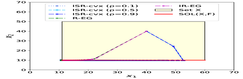
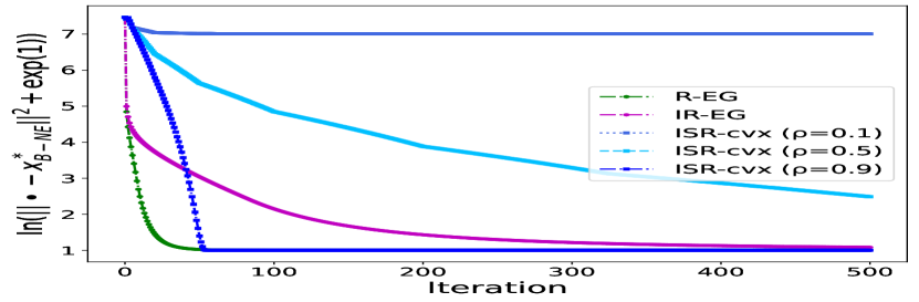
Figure 1: Computing the best NE using IR-EG, R-EG, and ISR-cvx. R-EG outperforms the other methods. ISR-cvx displays much sensitivity w.r.t. the decay parameter $\rho$.

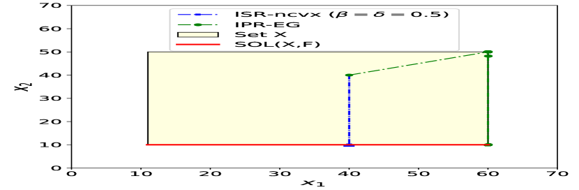
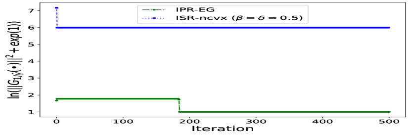
Figure 2: Computing the worst NE using IPR-EG and ISR-ncvx. IPR-EG converges to the unique worst NE. The iterate of ISR-ncvx is jammed in the set of equilibria.

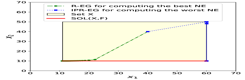
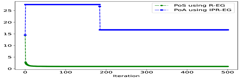
Figure 3: R-EG and IPR-EG successfully compute the PoS and PoA ratios, respectively.

(E1) In computing the best NE in Figure 1, R-EG outperforms the other schemes. This observation is indeed aligned with the accelerated rate statements provided in Corollary 3 for R-EG. The IR-EG method performs relatively fast, but slower than R-EG. This is because unlike in R-EG where we utilize the strong convexity of the objective function $f$, IR-EG is devised primarily for addressing merely convex objectives and it does not leverage the strong convexity property of $f$. As observed, the performance of ISR-cvx appears to be significantly sensitive to the decay factor $\rho$, emphasizing on the importance of the update rules for the regularization parameter. Indeed, one of the key contributions in our work is to provide prescribed update rules for the regularization parameter in the single-timescale methods IR-EG and R-EG.

(E2) In computing the worst NE in Figure 2, the sequence of iterates generated by IPR-EG appears to successfully converge to the unique stationary point $x^{*}_{{\tiny\mbox{W-NE}}}=(60,10)$. This is indeed aligned with the theoretical guarantees in Theorem 4. We observe, however, that the sequence of iterates generated by ISR-ncvx appears to converge to a vector in the set $\mbox{SOL}(X,F)$ that deviates from the worst NE. A similar observation was observed when we used different values for the initial point, $\beta$, or $\delta$. To plot the error in terms of the residual mapping, we use $\ln(\bullet+\exp(1))$ to better present the performance of the metric when the residual mapping is approaching zero. Notably, even though both methods start from the same initial point, the initial residual mapping takes different values between the two methods. This is because, unlike in IPR-EG where a constant stepsize is used, ISR-ncvx leverages a line search technique to find a suitable stepsize at each iteration.

(E3) Lastly, in Figure 3, we observe that the PoS ratio approximated by R-EG and PoA ratio approximated by IPR-EG converge to their true values, i.e., $1$ and $16.74$, respectively, as evaluated earlier. We note that in this particular experiment, the stationary point to the worst-NE seeking problem is unique. In general, however, a stationary point may not necessarily be among the worst equilibria.

5 Concluding remarks

In noncooperative game theory, understanding the quality of Nash equilibrium has been a storied area of research and has led to the emergence of popular metrics including the Price of Anarchy and the Price of Stability. The evaluation of these ratios is complicated by the need to compute the worst and the best equilibrium, respectively. In this paper, our goal is to devise a class of iteratively regularized extragradient methods with performance guarantees for computing the optimal equilibrium. To this end, we consider optimization problems with merely monotone variational inequality (VI) constraints when the objective function is either (i) merely convex, (ii) strongly convex, or (iii) nonconvex. In (i), we considerably improve the existing complexity guarantees. In (ii) and (iii), we derive new complexity guarantees for solving this class of problems. Notably, this appears to be the first work where nonconvex optimization with monotone VI constraints is addressed with complexity guarantees. We further show that our results in (i) and (ii) can be generalized to address a class of bilevel VIs that subsumes challenging problem classes such as the generalized Nash equilibrium problem. Extensions of the results in this work to stochastic regimes are among interesting directions for future research.

Appendix A Supplementary material

Lemma 7.

Consider problem Eq. 4 and let $X$ and $F$ be given by Eq. 6 where the set $Y\subseteq\mathbb{R}^{p}$ is closed and convex and functions $g$, $h_{j}$, $j=1,\ldots,q$ are continuously differentiable and convex. Then, the mapping $F$ is merely monotone on $X$.

Proof.

Suppose $x_{1},x_{2}\in X$ are arbitrary given vectors. From Eq. 6, we can write

$$(F(x_{1})-F(x_{2}))^{T}(x_{1}-x_{2}) =(\nabla g(y_{1})-\nabla g(y_{2}))^{T}(y_{1}-y_{2})$$

$$+\sum_{j=1}^{q}(\nabla h_{j}(y_{1})\lambda_{1,j}-\nabla h_{j}(y_{2})\lambda_{2,j})^{T}(y_{1}-y_{2})$$

$$+\sum_{j=1}^{q}(h_{j}(y_{2})-h_{j}(y_{1}))(\lambda_{1,j}-\lambda_{2,j}),$$

where $\lambda_{1,j}$ and $\lambda_{2,j}$ denote the $j$th dual variable in $x_{1}$ and $x_{2}$, respectively. Let us define $\mathcal{J}_{+}\triangleq\{j\in[q]\mid\lambda_{1,j}-\lambda_{2,j}\geq 0\}$ and $\mathcal{J}_{-}\triangleq\{j\in[q]\mid\lambda_{1,j}-\lambda_{2,j}<0\}$. Then, adding and subtracting the two terms $\sum_{j\in\mathcal{J}_{+}}\nabla h_{j}(y_{1})\lambda_{2,j}$ and $\sum_{j\in\mathcal{J}_{-}}\nabla h_{j}(y_{2})\lambda_{1,j}$, we obtain

$$(F(x_{1})-F(x_{2}))^{T}(x_{1}-x_{2})=(\nabla g(y_{1})-\nabla g(y_{2}))^{T}(y_{1}-y_{2})$$

$$+\sum_{j\in\mathcal{J}_{+}}^{q}(\nabla h_{j}(y_{1})\lambda_{1,j}-\nabla h_{j}(y_{1})\lambda_{2,j}+\nabla h_{j}(y_{1})\lambda_{2,j}-\nabla h_{j}(y_{2})\lambda_{2,j})^{T}(y_{1}-y_{2})$$

$$+\sum_{j\in\mathcal{J}_{-}}^{q}(\nabla h_{j}(y_{1})\lambda_{1,j}-\nabla h_{j}(y_{2})\lambda_{1,j}+\nabla h_{j}(y_{2})\lambda_{1,j}-\nabla h_{j}(y_{2})\lambda_{2,j})^{T}(y_{1}-y_{2})$$

$$+\sum_{j=1}^{q}(h_{j}(y_{2})-h_{j}(y_{1}))(\lambda_{1,j}-\lambda_{2,j}).$$

Rearranging the terms, we obtain

$$(F(x_{1})-F(x_{2}))^{T}(x_{1}-x_{2})=(\nabla g(y_{1})-\nabla g(y_{2}))^{T}(y_{1}-y_{2})$$

$$+\sum_{j\in\mathcal{J}_{+}}^{q}(\lambda_{1,j}-\lambda_{2,j})\nabla h_{j}(y_{1})^{T}(y_{1}-y_{2})+\sum_{j\in\mathcal{J}_{+}}^{q}\lambda_{2,j}(\nabla h_{j}(y_{1})-\nabla h_{j}(y_{2}))^{T}(y_{1}-y_{2})$$

$$+\sum_{j\in\mathcal{J}_{-}}^{q}\lambda_{1,j}(\nabla h_{j}(y_{1})-\nabla h_{j}(y_{2}))^{T}(y_{1}-y_{2})+\sum_{j\in\mathcal{J}_{-}}^{q}(\lambda_{1,j}-\lambda_{2,j})\nabla h_{j}(y_{2})^{T}(y_{1}-y_{2})$$

$$+\sum_{j=1}^{q}(h_{j}(y_{2})-h_{j}(y_{1}))(\lambda_{1,j}-\lambda_{2,j}).$$

From the nonnegativity of the Lagrange multipliers and convexity of functions $g$ and $h_{j}$, we have

$$(F(x_{1})-F(x_{2}))^{T}(x_{1}-x_{2})\geq$$

$$+\sum_{j\in\mathcal{J}_{+}}^{q}(\lambda_{1,j}-\lambda_{2,j})\left(h_{j}(y_{2})-h_{j}(y_{1})+\nabla h_{j}(y_{1})^{T}(y_{1}-y_{2})\right)$$

$$+\sum_{j\in\mathcal{J}_{-}}^{q}(\lambda_{1,j}-\lambda_{2,j})\left(h_{j}(y_{2})-h_{j}(y_{1})+\nabla h_{j}(y_{2})^{T}(y_{1}-y_{2})\right).$$

In view of convexity of $h_{j}$, we have that $h_{j}(y_{2})-h_{j}(y_{1})+\nabla h_{j}(y_{1})^{T}(y_{1}-y_{2})\geq 0$ and $h_{j}(y_{2})-h_{j}(y_{1})+\nabla h_{j}(y_{2})^{T}(y_{1}-y_{2})\leq 0$. Invoking the definitions of $\mathcal{J}_{+}$ and $\mathcal{J}_{-}$, we have $(F(x_{1})-F(x_{2}))^{T}(x_{1}-x_{2})\geq 0$ and thus, $F$ is merely monotone on $X$. ∎

Lemma 8 ([25, Lemma 2.14]).

Let $\alpha\in[0,1)$ and $K\geq 1$ be an integer. Then for all $K\geq{2}^{1/(1-\alpha)}$, we have $\frac{{K}^{1-\alpha}}{2(1-\alpha)}\leq\textstyle\sum_{k=0}^{K-1}(k+1)^{-\alpha}\leq\frac{K^{1-\alpha}}{1-\alpha}.$

Lemma 9 ([47, Lemma 9]).

For any scalar $\alpha$ and integers $\ell$ and $N$ where $0\leq\ell\leq N-1$, the following results hold.

• $\ln\left(\frac{N+1}{\ell+1}\right)\leq\sum_{k=\ell}^{N-1}\frac{1}{k+1}\leq\frac{1}{\ell+1}+\ln\left(\frac{N}{\ell+1}\right)$.

• $\frac{N^{\alpha+1}-(\ell+1)^{\alpha+1}}{\alpha+1}\leq\sum_{k=\ell}^{N-1}(k+1)^{\alpha}\leq(\ell+1)^{\alpha}+\frac{(N+1)^{\alpha+1}-(\ell+1)^{\alpha+1}}{\alpha+1}$, for $\alpha\neq-1$.

References

- [1] A. Alacaoglu and Y. Malitsky, Stochastic variance reduction for variational inequality methods, in Conference on Learning Theory, PMLR, 2022, pp. 778–816.
- [2] Z. Alizadeh, A. Jalilzadeh, and F. Yousefian, Randomized lagrangian stochastic approximation for large-scale constrained stochastic Nash games, arXiv preprint arXiv:2304.07688, (2023).
- [3] M. Amini and F. Yousefian, An iterative regularized mirror descent method for ill-posed nondifferentiable stochastic optimization, arXiv preprint arXiv:1901.09506, (2019).
- [4] E. Anshelevich, A. Dasgupta, J. Kleinberg, É. Tardos, T. Wexler, and T. Roughgarden, The price of stability for network design with fair cost allocation, SIAM Journal on Computing, 38 (2008), pp. 1602–1623.
- [5] A. Beck, First-Order Methods in Optimization, Society for Industrial and Applied Mathematics, Philadelphia, PA, 2017, https://doi.org/10.1137/1.9781611974997.
- [6] A. Beck and S. Sabach, A first order method for finding minimal norm-like solutions of convex optimization problems, Mathematical Programming, 147 (2014), pp. 25–46.
- [7] E. Benenati, W. Ananduta, and S. Grammatico, Optimal selection and tracking of generalized Nash equilibria in monotone games, IEEE Transactions on Automatic Control, (2023).
- [8] E. Benenati, W. Ananduta, and S. Grammatico, A semi-decentralized tikhonov-based algorithm for optimal generalized nash equilibrium selection, arXiv preprint arXiv:2304.12793, (2023).
- [9] D. Bertsekas, A. Nedić, and A. Ozdaglar, Convex analysis and optimization, vol. 1, Athena Scientific, 2003.
- [10] D. Chan and J. Pang, The generalized quasi-variational inequality problem, Mathematics of Operations Research, 7 (1982), pp. 211–222.
- [11] L. Chen, J. Xu, and J. Zhang, On bilevel optimization without lower-level strong convexity, arXiv preprint arXiv:2301.00712, (2023).
- [12] F. Facchinei and C. Kanzow, Generalized Nash equilibrium problems, Annals of Operations Research, 175 (2010), pp. 177–211.
- [13] F. Facchinei and J.-S. Pang, Finite-dimensional Variational Inequalities and Complementarity Problems. Vols. I,II, Springer Series in Operations Research, Springer-Verlag, New York, 2003.
- [14] F. Facchinei, J.-S. Pang, G. Scutari, and L. Lampariello, VI-constrained hemivariational inequalities: distributed algorithms and power control in ad-hoc networks, Mathematical Programming, 145 (2014), pp. 59–96.
- [15] Z. Feinstein and B. Rudloff, Characterizing and computing the set of Nash equilibria via vector optimization, Operations Research, (2023).
- [16] M. C. Ferris and O. L. Mangasarian, Finite perturbation of convex programs, Applied Mathematics and Optimization, 23 (1991), pp. 263–273.
- [17] M. P. Friedlander and P. Tseng, Exact regularization of convex programs, SIAM Journal on Optimization, 18 (2008), pp. 1326–1350.
- [18] A. N. Iusem, A. Jofré, R. I. Oliveira, and P. Thompson, Extragradient method with variance reduction for stochastic variational inequalities, SIAM Journal on Optimization, 27 (2017), pp. 686–724.
- [19] A. Jalilzadeh, F. Yousefian, and M. Ebrahimi, Stochastic approximation for estimating the price of stability in stochastic Nash games, arXiv:2203.01271, (2023).
- [20] H. Jiang and H. Xu, Stochastic approximation approaches to the stochastic variational inequality problem, IEEE Transactions on Automatic Control, 53 (2008), pp. 1462–1475.
- [21] R. Jiang, N. Abolfazli, A. Mokhtari, and E. Y. Hamedani, A conditional gradient-based method for simple bilevel optimization with convex lower-level problem, in International Conference on Artificial Intelligence and Statistics, PMLR, 2023, pp. 10305–10323.
- [22] A. Juditsky, A. Nemirovski, and C. Tauvel, Solving variational inequalities with stochastic mirror-prox algorithm, Stochastic Systems, 1 (2011), pp. 17–58.
- [23] A. Kannan and U. V. Shanbhag, Optimal stochastic extragradient schemes for pseudomonotone stochastic variational inequality problems and their variants, Computational Optimization and Applications, 74 (2019), pp. 779–820.
- [24] H. D. Kaushik, S. Samadi, and F. Yousefian, An incremental gradient method for optimization problems with variational inequality constraints, IEEE Transactions on Automatic Control, (2023), https://doi.org/10.1109/TAC.2023.3251851.
- [25] H. D. Kaushik and F. Yousefian, A method with convergence rates for optimization problems with variational inequality constraints, SIAM Journal on Optimization, 31 (2021), pp. 2171–2198, https://doi.org/10.1137/20M1357378.
- [26] D. Kinderlehrer and G. Stampacchia, An introduction to variational inequalities and their applications, SIAM, 2000.
- [27] G. M. Korpelevich, The extragradient method for finding saddle points and other problems, Matecon, 12 (1976), pp. 747–756.
- [28] G. Kotsalis, G. Lan, and T. Li, Simple and optimal methods for stochastic variational inequalities, I: operator extrapolation, SIAM Journal on Optimization, 32 (2022), pp. 2041–2073.
- [29] E. Koutsoupias and C. Papadimitriou, Worst-case equilibria, in Annual symposium on theoretical aspects of computer science, Springer, 1999, pp. 404–413.
- [30] L. Lampariello, G. Priori, and S. Sagratella, On the solution of monotone nested variational inequalities, Mathematical Methods of Operations Research, 96 (2022), pp. 421–446.
- [31] P. Latafat, A. Themelis, S. Villa, and P. Patrinos, AdaBiM: An adaptive proximal gradient method for structured convex bilevel optimization, arXiv preprint arXiv:2305.03559, (2023).
- [32] P. Marcotte and D. Zhu, Weak sharp solutions of variational inequalities, SIAM Journal on Optimization, 9 (1998), pp. 179–189.
- [33] R. Merchav and S. Sabach, Convex bi-level optimization problems with non-smooth outer objective function, arXiv preprint arXiv:2307.08245, (2023).
- [34] A. Nemirovski, Prox-method with rate of convergence o (1/t) for variational inequalities with lipschitz continuous monotone operators and smooth convex-concave saddle point problems, SIAM Journal on Optimization, 15 (2004), pp. 229–251.
- [35] C. Papadimitriou, Algorithms, games, and the internet, in Proceedings of the thirty-third annual ACM symposium on Theory of computing, 2001, pp. 749–753.
- [36] R. T. Rockafellar and R. J.-B. Wets, Variational analysis, vol. 317, Springer Science & Business Media, 2009.
- [37] S. Sabach and S. Shtern, A first order method for solving convex bilevel optimization problems, SIAM Journal on Optimization, 27 (2017), pp. 640–660.
- [38] L. Shen, N. Ho-Nguyen, and F. Kılınç-Karzan, An online convex optimization-based framework for convex bilevel optimization, Mathematical Programming, 198 (2023), pp. 1519–1582.
- [39] M. Solodov, An explicit descent method for bilevel convex optimization, Journal of Convex Analysis, 14 (2007), p. 227.
- [40] M. V. Solodov, A bundle method for a class of bilevel nonsmooth convex minimization problems, SIAM Journal on Optimization, 18 (2007), pp. 242–259.
- [41] D. V. Thong, N. A. Triet, X.-H. Li, and Q.-L. Dong, Strong convergence of extragradient methods for solving bilevel pseudo-monotone variational inequality problems, Numerical Algorithms, 83 (2020), pp. 1123–1143.
- [42] A. N. Tikhonov, On the solution of ill-posed problems and the method of regularization, in Doklady akademii nauk, vol. 151, Russian Academy of Sciences, 1963, pp. 501–504.
- [43] D. Van Hieu and A. Moudafi, Regularization projection method for solving bilevel variational inequality problem, Optimization Letters, 15 (2021), pp. 205–229.
- [44] I. Yamada and N. Ogura, Hybrid steepest descent method for variational inequality problem over the fixed point set of certain quasi-nonexpansive mappings, (2005).
- [45] F. Yousefian, Bilevel distributed optimization in directed networks, in 2021 American Control Conference (ACC), IEEE, 2021, pp. 2230–2235.
- [46] F. Yousefian, A. Nedić, and U. V. Shanbhag, Optimal robust smoothing extragradient algorithms for stochastic variational inequality problems, in 53rd IEEE conference on decision and control, IEEE, 2014, pp. 5831–5836.
- [47] F. Yousefian, A. Nedić, and U. V. Shanbhag, On smoothing, regularization, and averaging in stochastic approximation methods for stochastic variational inequality problems, Mathematical Programming, 165 (2017), pp. 391–431.
- [48] F. Yousefian, A. Nedić, and U. V. Shanbhag, On stochastic mirror-prox algorithms for stochastic cartesian variational inequalities: Randomized block coordinate and optimal averaging schemes, Set-Valued and Variational Analysis, 26 (2018), pp. 789–819.