The Temporal Symmetrical and Translational Structure in Gamma-Ray Burst Light Curves

Abstract

Tremendous information is hidden in the light curve of a gamma-ray burst (GRB). Based on CGRO/BATSE data, Hakkila (2021) found a majority of GRBs can be characterized by a smooth, single-peaked component superposed with a temporally symmetrical residual structure, i.e., a mirror feature for the fast varying component. In this study, we conduct a similar analysis on the same data, as well as on Fermi/GBM data. We got a similar conclusion that most GRBs have this symmetrical fast varying component. Further more, we chose an alternative model to characterize the smooth component and used a three-parameter model to identify the residual, i.e., the fast component. By choosing 226 BATSE GRBs based on a few criteria, we checked the time symmetrical feature and time translational feature for the fast components and found the ratio is roughly 1:1. We propose that both features could come from the structure of the ejected shells. Future SKA might be able to observe the early radio emission from the collision of the shells.

1 Introduction

Gamma-ray bursts (GRBs) are among the most powerful explosions in the universe, with duration ranging from less than 0.01 seconds to more than 1000 seconds. The isotropic energy emitted in $\gamma$-rays can be as high as $10^{48}-10^{55}$ ergs. GRBs are observed to consist of two different phases: the prompt emission, which is concentrated in the keV-MeV energy range, and the afterglow, which extends from $\gamma$-rays to the radio band (Mészáros, 2006; Kumar & Zhang, 2015). According to the fireball model, GRBs are produced by highly relativistic and collimated jets, and the prompt emission is the result of the kinetic energy dissipated in internal collisions, while the afterglow is produced by the interaction of the jet with the ambient material (Piran, 1999, 2004).

As the nature of GRBs is not completely understood, studying their light curves may provide useful information. In this paper, we focus on the light curve of prompt emission. Most GRB light curves are highly variable, with variability timescales that can be as short as milliseconds (MacLachlan et al., 2012). However, there are also about $20\%$ of bursts that show a smooth pulse, which can generally be fitted by a fast rise exponential decay (FRED) model (Norris et al., 1996; Lee et al., 2000a, b; Kocevski et al., 2003). According to the internal-shock model, a GRB light curve is composed of many individual pulses, with every individual pulse corresponding to a collision between individual shells (Norris et al., 1996; Kobayashi et al., 1997). However, there are also models and studies believe that GRB pulses can be made up of two components, a smooth component and a more variable component. Vetere et al. (2006) considered the two components as a slow component and a fast component and found that the slow component is generally softer than the fast ones. Zhang & Yan (2011) proposed the Internal-Collision-induced MAgnetic Reconnection and Turbulence (ICMART) model, which also prefers the two-component scenario. Gao et al. (2012) developed a new method to identify significant clustering structures of a light curve in the frequency domain and found that the majority of bursts have clear evidence of such a superposition effect.

In a study of a dataset of GRBs from the Burst And Transient Source Experiment (BATSE) at NASA’s Compton Gamma Ray Observatory (Band et al., 1993), Hakkila (2021) found that a majority of GRB pulses could be characterized by a smooth, single-peaked component coupled with a temporally symmetrical residual structure. This finding is intriguing as it provides further evidence that GRB light curves may indeed have two components. Additionally, the temporal symmetry of the residual structure is unexpected and has not been predicted by any existing model to our knowledge. Very recently, Moussa et al. (2023) observed the time reflection effect in laboratory. It could be a clue for understanding the temporally symmetrical effect in GRB light curves.

We aim to investigate the existence of the symmetrical signal and determine its nature. In this study, we follow the method employed by Hakkila (2021) to confirm the time symmetry of the residual and expand the data set by using data from the Gamma-ray Burst Monitor (GBM) aboard the Fermi Gamma-ray Space Telescope (Meegan et al., 2009). We also modify the method to mitigate the influence of the slow component and propose a three-parameter model to characterize the residual. Finally, we attempt to interpret this phenomenon using the internal-external shock model.

In this paper, we first introduce the method in Hakkila (2021) for characterizing a GRB light curve, and present our results based on our data selection in Section 2. In Section 3, we discuss limitations of the original model and propose a new model to further investigate this symmetry. Section 4 presents the findings of our new model. We also propose a possible explanation for the phenomenon in Section 5. Finally, we conclude and discuss our findings in Section 6.

2 The original model and results

2.1 Method

We will briefly introduce the method used in Hakkila (2021) first. For a given GRB light curve, the monotonic component of the GRB pulse can be modeled by fitting the light curve using a simple, generic mathematical model. The pulse model is based on the pulse intensity function of Norris et al. (2005), which can be described as

$$I(t)=A\lambda e^{[-\tau_{1}/(t-t_{s})-(t-t_{s})/\tau_{2}]},$$ (1)

where $t$ is the time since trigger, $A$ is the amplitude of the pulse, $t_{s}$ is the pulse start time, $\tau_{1}$ is the pulse rise parameter, $\tau_{2}$ is the pulse decay parameter, and $\lambda$ is a normalization constant. Since not all GRB pulse light curves can be fitted by this function, the remaining light curves are fitted using a Gaussian distribution function of the form

$$I(t)=\frac{C}{\sigma\sqrt{2\pi}}{\rm exp}[-(\frac{t-t_{0}}{\sqrt{2}\sigma})^{2}],$$ (2)

where $C$ is the pulse amplitude, $t_{0}$ is the time when $C$ occurs, and $\sigma^{2}$ is the variance. The pulse duration window can be defined by the pulse starting time $t_{start}$ and the pulse end time $t_{end}$, both of which are measured at $I_{meas}/I_{peak}=e^{-3}$. A background model is also required with a simple form

$$B=B_{0}+BS\times{t},$$ (3)

where $B_{0}$ is the mean background, and $BS$ is the rate of change of the background. After fitting the monotonic component, the residual, which are considered to be temporally symmetric, can be obtained by subtracting this component from the data. Two parameters are required to characterize the residual: the time $t_{0;mirror}$ at which the forward and backward residuals are symmetrical and the stretching parameter $s_{mirror}$, which represents the ratio between time-forward structures and time-reversed structures. Both of these parameters are determined by the maximum value of the normalized cross-correlation function (CCF):

$${\rm CCF}=\frac{\sum_{i}(x_{i}-\overline{x})(y_{i}-\overline{y})}{\sqrt{\sum_{i}(x_{i}-\overline{x})^{2}}\sqrt{\sum_{i}(y_{i}-\overline{y})^{2}}}.$$ (4)

In other words, after obtaining the residual, then the CCF is applied to the folded time-forward part and time-reversed parts with varying $t_{0;mirror}$ and $s_{mirror}$ values to search for the maximum CCF value, which indicates the best match between the time-forward and time-reversed parts. Note that the existence of $s_{mirror}$ results in different bin widths between the two parts, linear interpolation is employed on the folded part of the residual light curve. Data resampling is used for error estimation (Andrae, 2010). Different $t_{0;mirror}$ and $s_{mirror}$ are generated by adding random Poisson noise to the light curve. The distribution of parameters are used to evaluate their uncertainties. A GRB light curve with $\sigma_{s,mirror}<0.4$ can be directly classified as temporally symmetric. Besides, a residual statistic, given by

$$R=\sqrt{\frac{\sigma_{res}}{\langle B\rangle}},$$ (5)

is introduced to quantify the brightness of the residual structure. Additionally, the $p$-value obtained from a $\chi^{2}$ test on the pulse fitting is required to assess the quality of the fitting result.

For a more detailed description and the criterion of temporally symmetry, please refer to Hakkila & Preece (2014), Hakkila et al. (2018) and Hakkila (2021).

A typical fitting result is presented in Figure 1,

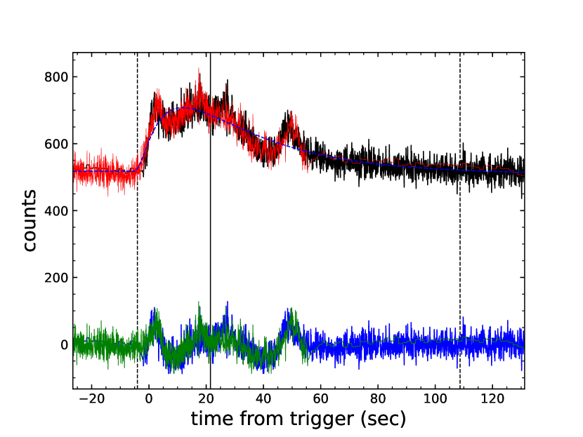
Figure 1: Temporally symmetric model fits to BATSE pulse 659 light curve. The figure shows the counts data in black line, the fit to the monotonic component in blue dashed line, the time-reversed model in red line, the residual in blue line, the time-reversed residual in green line, the duration window from $t_{start}$ to $t_{end}$ (vertical dashed lines), and the time of reflection $t_{0;mirror}$ (vertical solid line).

which shows the model applying to BATSE pulse 659. The fitting looks well. The residual structure shows time symmetry with the maximum CCF of residual ${\rm CCF}_{resids}=0.468$ and $t_{0;mirror}=21.49$, $s_{mirror}=0.69$. By resampling the data and using Monte Carlo simulation, a seires of $t_{0;mirror}$ and $s_{mirror}$ can be generated for error estimation. For BATSE pulse 659, a $\sigma_{s,mirror}$ of 0.14 is obtained, indicating that it is a temporally symmetrical light curve.

2.2 Data selection

In this work, we analyze two different GRB data samples obtained from BATSE and GBM, respectively. The following section provides a brief description of each data set.

We repeat Hakkila’s results using the same BATSE data set as in Hakkila (2021), but conduct data filtering. Our data comes exclusively from BATSE’s 64 ms resolution data , and we do not attempt to analyze the 4 ms data, since the proportion of such data is very small in the original data set and would not significantly affect the results. We remove data considered to be multiple pulses in Hakkila (2021). These GRBs are believed to have multiple emission episodes, which make it inappropriate to treat them as a single GRB. Therefore, it is necessary to segment the data. Since we do not have the specific parameters used by the original authors for segmentation, we decided to discard these data. These data may have no much impact on the final results or proportions. Our sample includes 226 GRBs out of the 312 BATSE GRBs, allowing us to replicate previous results.

We further consider Fermi GBM data of the years 2020 and 2021. We downloaded the time-tagged event (TTE) data for approximately 600 GRBs from the Fermi Science Support Center (FSSC) FTP website . GBM comprises 12 sodium iodide (NaI) detectors and 2 bismuth germanate (BGO) detectors. For each GRB, we select the TTE data from the triggered NaI detectors since they are typically the brightest ones. Subsequently, we combine the data from these detectors to extract the 64 ms light curve data. The data extraction process is performed using the GBM Data Tools , a software package provided by the FSSC.

Although the energy ranges and time scales of the data from the BATSE and GBM instruments differ, considering that our research focus is on the overall morphology of the light curves, the impact of energy ranges and time scales is not significant.

2.3 Results

By following the procedures outlined in Section 2.1, GRBs can be categorized into three groups depending on their conformity to the temporally symmetric model. Utilizing the data sample detailed in Section 2.2, we present our statistical outcomes in Table 1. To facilitate comparison, we list the findings of Hakkila (2021) in the initial row. The data selected from Hakkila (2021) were unbiased. To demonstrate this, we have listed the same data distribution in Hakkila (2021) in the second row. The symmetry ratio of the new sample is nearly consistent with that of the original sample. Followed by our outcomes acquired from the identical BATSE data and new data from GBM.

Our findings reveal that the temporally symmetric model was able to successfully fit $85\%$ of the BATSE GRBs, which is highly consistent with the previous results reported by Hakkila (2021). However, when using the data obtained from GBM, we observed a significant difference in the distribution of results, with the majority of the data being classified as monotonic. This difference could be attributed to the fact that the effective detection area corresponding to the GBM data in our sample is considerably smaller than that of the BATSE, resulting in a lower signal-to-noise ratio of the majority of the GRBs detected by GBM and less distinct structures, which lead to a smaller residual statistic $R$. Nonetheless, the proportion of monotonic GRBs does not affect the symmetry ratio. Among the remaining GRBs, the proportion is over $70\%$, which although lower than before, is still relatively high.

The fitting parameters and corresponding results for the data from both instruments are presented in Tables LABEL:tab:2 and LABEL:tab:3 in the appendix. It should be noted that for the GBM data, we only report the results for the other two types of pulses as there were a large number of monotonic pulses identified that do not contribute to the determination of the symmetry ratio. It is worth mentioning that the absence of pre-screening of the GBM data may introduce biases, which could potentially be a contributing factor to the lower symmetry ratio observed in the GBM data.

Table 1: The Results of Temporal Symmetry Pulse Fitting

Data set	Not temporally symmetric	Monotonic	Temporally symmetric	Symmetry ratio
BATSE (Hakkila, 2021)	25	126	161	$86.6\%$
BATSE with filter	21	83	122	$85.3\%$
BATSE	18	106	102	$85.0\%$
GBM 64 ms (2020)	14	195	39	$73.6\%$
GBM 64 ms (2021)	11	170	37	$77.1\%$

Note. —

3 A new model

Another issue highlighted in Hakkila (2021) is that the assumption of temporal symmetry may not fully capture the shape of residual structures. This can be seen in Figure 2, where we manually generate two types of residuals corresponding to the time-symmetrical and time-translational cases. The red curve represents the original data, which we then perturb with Poisson noise to obtain the blue curve. The green curve is the time-reversed residual determined by the maximum value of CCF. Through Monte Carlo simulations, we find that the calculated value of $\sigma_{s,mirror}$ is small enough in both cases to be defined as temporally symmetric. This means that the original model can only characterize the symmetry of pulse orders in the fast-varying structure but cannot capture the symmetry of the pulse shapes. Therefore, building upon the original model, we design a new model that characterizes the residuals. Under this model, we can provide a comparison of pulse shape symmetry and translation. For convenience, we refer to these models as the symmetrical model and translational model, respectively. We expect the symmetrical model outperforms the translational model, which indicates that symmetry exists not only in the pulse order but also in the pulse shapes.

The details of the new model are described in the following subsections.

3.1 Characterizing the monotonic component

Several studies have proposed models that describe GRB pulses as a combination of slow and fast components (Vetere et al., 2006; Zhang & Yan, 2011; Gao et al., 2012). This aligns closely with the viewpoint of Hakkila (2021) that GRBs can be characterized by a smooth, single-peaked component superposed with a temporally symmetrical residual structure. By combining the two, it naturally leads us to hypothesize that the fitting to the monotonic component represents the slow component and the residual represent the fast component. Additionally, the unique properties of the fast component can distinguish it from the slow component.

If both the fast component and the slow component are from some certain radiation processes, i.e., not absorption as the non-thermal spectra in most cases, we do not expect any of them are significantly below zero. However, a direct fitting to the GRB light curve can leave residual component that are obviously below zero. The left panel of Figure 3 shows a direct fitting to BATSE pulse 109. According to our hypothesis, the monotonic component should be lower than the fitting result, but due to the existence of the fast component, the fitting result is raised, leaving a residual that does not meet our expectations. In other words, due to the presence of fast-varying components, the fitting of slow-varying components can be overestimated, leading to an underestimation of the fast-varying components in the results. Representing the slow-varying component solely based on direct fitting results is inadequate.

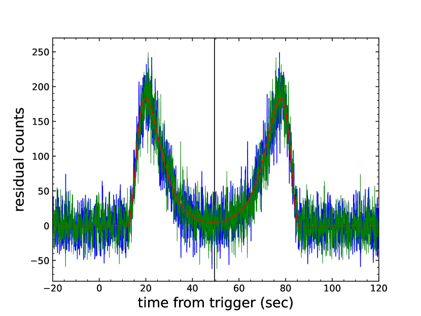
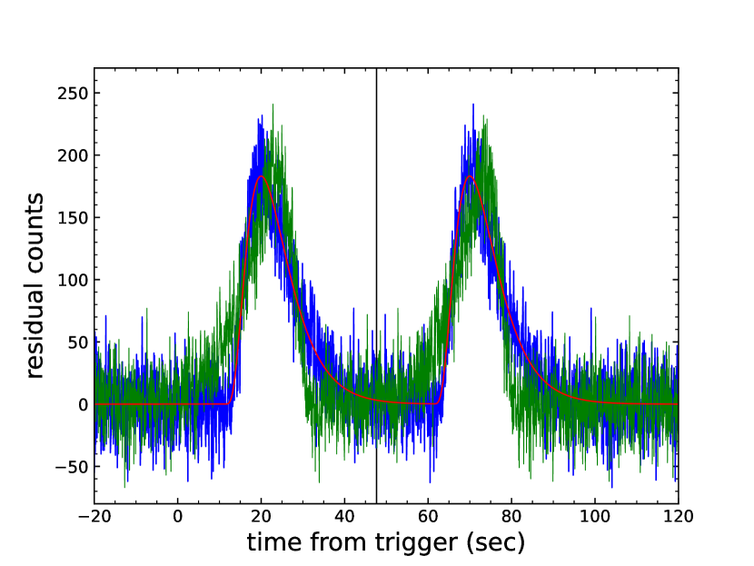
Figure 2: Synthetic residuals and fitting results. Including the signal in red, the signal with noise in blue, the time-reversed residuals in green, the time-symmetrical residual in the left panel and the time-translational residual in the right panel.

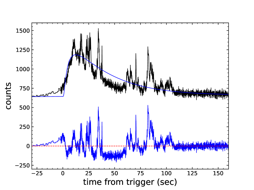
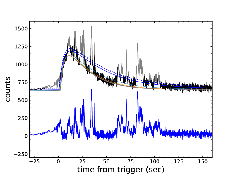
Figure 3: Two fitting approaches apply to BATSE pulse 109, a direct fitting (left panel) which produce the undesirable residual and the iterative fitting (right panel). The figure shows the counts data in black line, the fit to the Norris/Gaussian model in colored solid lines, the residual in blue line, and a zero horizontal line in red dashed line.

To address this problem, we have developed a simple yet effective method. We continue to use the FRED function in Norris et al. (2005) or Gaussian distribution function as the basis of the pulse model. The difference is that we will perform iterative fitting. After each fitting, the data points that are above the noise level of the fitting curve will be masked and the rest of the data will be used for the next fitting, until the fitting results converge. The parameter results of the last fitting are taken as the initial value of the next fitting. The noise level is estimated simply by taking the square root of the signal. In the right panel of Figure 3. Initially, we perform a fitting on the entire light curve, resulting in the blue solid line. Using this blue solid line, we obtain the critical line, represented by the blue dotted line in the graph. The data points above the critical line, represented by the gray region, will be removed. Then the remaining data points are used for the second round of fitting and critical line assessment. As the iteration progress, the number of removed data points gradually decrease, and eventually, the fitting line remain relatively stable, indicating convergence. For BATSE pulse 109, the final fitting curve converges to the expected contour after 9 iterations. The valleys of residual show Poisson variations near zero. Notice that the iterative fitting is the main difference from Hakkila’s method. The consequence is that the negative part in the light curve never appear in our treatment. This treatment implies an assumption that there is no absorption, and all the emissions are from optically thin regions. Using this method, we obtain the fitting results of the monotonic/slow component of GRBs, which are shown in Table LABEL:tab:4 in the appendix.

3.2 Three-parameter residual model

We try to perform comparative experiments between the translational model and the symmetrical model to explore the presence of symmetry in the pulse shapes of the fast-varying component. After some attempts, we have found that it is difficult to define the translational model with only two parameters. Once the residual of a GRB light curve are obtained, the $t_{mirror}$ can divide the residual into two parts. For the symmetrical model, the tail of the left residual is automatically aligned with the head of the right residual. However, for the translational model, what we can do is to move the left part until $t_{start}$ and $t_{mirror}$ coincide, which does not work for residuals with a long smooth head. Therefore, we introduce a three-parameter model to solve this problem. The three parameters are splitting time $t$, translation parameter $\Delta t$, and stretching parameter $s$. The translational model is characterized as follows.

The residual are obtained using the method described in Section 3.1. Subsequently, the residual are divided into two parts by selecting a splitting time $t$, and the left residual are translated by a translation parameter $\Delta t$ and stretched by a stretching parameter $s$ until the maximum value of the CCF is achieved. It is important to note that we adopt a new form of CCF with a no-mean subtracted definition, expressed as

$${\rm CCF_{Band}}=\frac{\sum_{i}x_{i}y_{i}}{\sqrt{\sum_{i}x_{i}^{2}}\sqrt{\sum_{i}y_{i}^{2}}},$$ (6)

which is considered more suitable for transient events such as GRBs (Band, 1997; Ukwatta et al., 2010).

To maintain the same degrees of freedom between the symmetrical model and the translational model, a translation parameter is also introduced into the symmetrical model. The symmetrical model is characterized similarly to the translational model. The difference is that in symmetrical model, the residual on the left side needs to be folded and then align with the right side.

A more detailed description of the steps is provided below:

1. Choose a GRB pulse light curve and use iterative fitting to characterize the slow component. Subtract this component from the data to obtain the residual, which represent the fast component.

2. Cut off any residual data outside the duration window or replace it with zeros. Choose a splitting time $t$ to divide the residual into two parts.

3. Fold the left part of the residual in the symmetrical model, but not in the translational model. Translate the left part by $\Delta t$, stretch it by $s$, and calculate the ${\rm CCF_{Band}}$ with the right part.

4. Continuously adjust the model parameters to find the maximum value of the ${\rm CCF_{Band}}$.

When calculating the ${\rm CCF_{Band}}$, one side of the residual light curve and the projection from the other side form one of the two signals. The ${\rm CCF_{Band}}$ of the translational and symmetrical models are indicated by ${{\rm CCF}_{tm}}$ and ${{\rm CCF}_{sm}}$, respectively. The only difference between the two models is that the symmetrical model requires a folding operation while the translational model does not, allowing for a direct comparison between them. If there is also symmetry exist in the pulse shapes, we expect the symmetrical model to outperform the translational model, indicating that ${{\rm CCF}_{sm}>{\rm CCF}_{tm}}$ for the majority of GRBs.

To avoid the huge calculation resulting from traversing parameters, we adopted a global optimization algorithm known as Differential Evolution (Storn & Price, 1997). The differential evolution is a heuristic algorithm based on population evolution, similar to genetic algorithm. It has a simple structure, fast convergence, and strong robustness, and is commonly used for finding global optimal solutions for optimization problems characterized by nonlinear, multimodal, and high-dimensional relationships (Das & Suganthan, 2010). In this work, we refer to the publicly available code of scikit-opt to fit the residuals.

4 Results

The three-parameter residual model is applied to the BATSE data. The selected data are the same as Hakkila (2021). To avoid bias of human-eye, we removed the “multi-pulse” GRBs. To avoid the inconsistency of pulse definition, as well as the instrument selection effect, we do not include GBM data here. The resulting CCF values and parameter estimates for the symmetrical and translational models are listed in Table LABEL:tab:4. The subscripts “$sm$” and “$tm$” are used to denote the symmetrical and translational models, respectively.

Some visual results are presented in Figure 4.

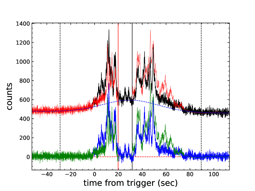
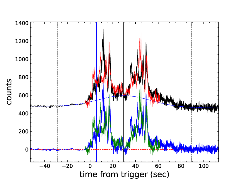
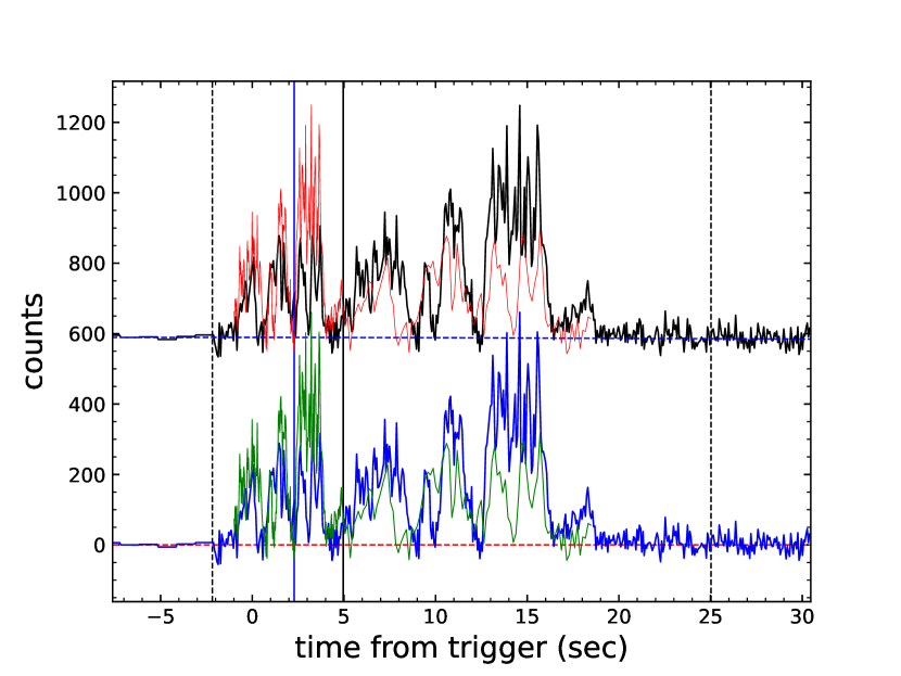
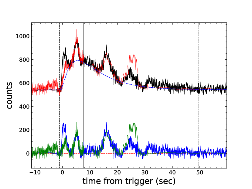
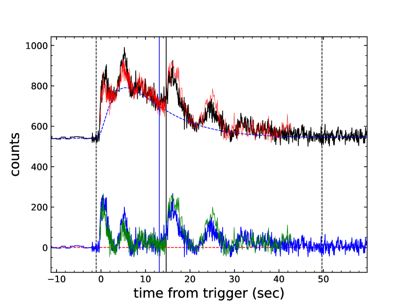
Figure 4: Three-parameter residual model applies on BATSE pulse 130, 160 and 548. The figure displays symmetrical and translational models for analyzing the three pulses, along with a blue dashed line representing the identified monotonic/slow component, a vertical dashed line indicating the pulse duration window, a black vertical line indicating the splitting time, and a red dashed line at the zero horizontal line. In the symmetrical model, the tail of the left residual ($t_{sm}$) moves to the red vertical line, while in the translational model, the head of the left part ($t_{start}$) moves to the blue vertical line.

The iterative fitting procedure is used to identify the slow component, and the fast component is obtained by subtracting it from the original data. The residual is then divided into two parts using the splitting time, and one part is translated and stretched to align with the other part. The green curve in the figure represents the fitting to the fast component, and it is added to the slow component to obtain the fitting of the whole light curve, which is represented by the red curve. We take BATSE pulses 130, 160, and 548 as examples since they all fit well with the original temporally symmetric model. In three-parameter residual model, all of them exhibit a high value of ${\rm CCF}_{sm}$, but as well as of ${\rm CCF}_{tm}$. The residual of BATSE pulse 130 exhibit two main peaks and the CCF results show that it is more suitable for the symmetrical model with ${\rm CCF}_{tm}=0.837$ and ${\rm CCF}_{sm}=0.901$. For BATSE pulse 160, iterative fitting shows that there is almost no slow component. This is a normal phenomenon. If the fast-varying and slow-varying components represent two independent radiation processes, it is possible for the slow-varying component to be too weak to be detected by the instrument, resulting in only the fast-varying component being observed. The maximum value of two models is almost equal with ${\rm CCF}_{tm}=0.832$ and ${\rm CCF}_{sm}=0.845$. However, in the symmetrical model, the light curve on each side is recognized as two peaks, while in the translational model, the light curve on one side appears to have three peaks. For BATSE pulse 548, there are four clear peaks in the residual, and the CCF results are ${\rm CCF}_{tm}=0.871$ and ${\rm CCF}_{sm}=0.739$, indicating that it is more suitable for the translational model.

The distribution of CCF values for 226 BATSE GRBs is presented in Figure 5. For each GRB, the parameter results and $\rm CCF_{Band}$ values of the two models are listed in Table LABEL:tab:3 in the appendix. The distribution of CCF values for both models showed no significant differences. We aim to investigate whether the results of the two models exhibit significant differences for a given GRB light curve. To achieve this, we calculate the difference between the ${\rm CCF}_{sm}$ and ${\rm CCF}_{tm}$ values for each GRB and display them as a column diagram in the lower panel of Figure 5. If one of the models is more appropriate for a given GRB, we expect to observe a distribution that deviates significantly from zero. However, our analysis reveals that the difference between the two models is negligible, with the results following a Gaussian distribution centered at zero. Out of the 226 BATSE GRB pulses analyzed, 114 show ${\rm CCF}_{sm}>{\rm CCF}_{tm}$ while 112 show ${\rm CCF}_{sm}<{\rm CCF}_{tm}$. Furthermore, the absolute difference between ${\rm CCF}_{sm}$ and ${\rm CCF}_{tm}$ for each GRB light curve is not greater than 0.2, indicating that the three-parameter symmetrical model does not provide a significant advantage over the three-parameter translational model. In other words, we have not found strong evidence to suggest that the pulse shapes of the fast-varying component also exhibit temporal symmetry. Approximately half of GRBs tend to show a preference for translation, while the other half tend to show a preference for symmetry.

While it is difficult to draw a universal conclusion regarding whether the residuals of most GRBs are better fit by a symmetrical or translational model, we have observed that some GRBs with distinct features are well-described by one of the two models. Specifically, BATSE pulse 109 and 121 show a high degree of consistency with the symmetrical model, while BATSE pulse 548 and 647 are well-described by the translational model. Both of the two models show the unique properties of fast components in GRB, and their mechanisms deserve further study.

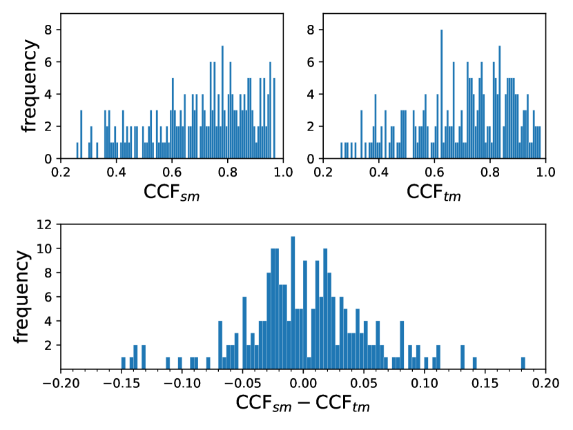
Figure 5: The distributions of the results for 226 BATSE GRBs. The figure displays the distribution of ${\rm CCF}_{tm}$ for the translational model (upper left panel), ${\rm CCF}_{sm}$ for the symmetrical model (upper right panel), and the distribution of the difference in CCF between the two models (lower panel).

5 Indication to the GRB scenario

Possible explanations for temporally symmetrical residuals have been proposed in Hakkila et al. (2018) and Hakkila & Nemiroff (2019), which mainly attribute the symmetry to the motion or material distribution of the emitting region. Additionally, it has been shown that superluminal motion may also produce a time-reversed signal (Nemiroff, 2018; Nemiroff & Kaushal, 2020).  Motivated by the reverse-forward shock model from Hakkila & Preece (2014), we suggest that symmetrical or translational signals may be produced by the following process.

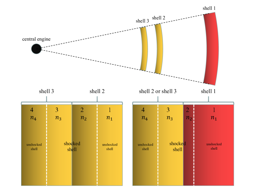
Figure 6: Schematic diagram of jet structure for the symmetrical and the translational temporal structure. Assume that the fast component of the emission are from shock front (white dashed line). It varies when the shock front sweeps to denser or rarer material. The symmetrical signal can be produced by the collision between shell 2 and shell 3 with similar structures, while the translational signal cab be produced by two similar shell collision onto a bigger outer shell.

As shown in Figure 6, intermittent activity of the central engine releases the shells. Assuming high density areas or lumps exist in both shell 2 and shell 3 with similar structures, which means the radial parameter distribution between the two shells is roughly the same. This may come from the similarity of the central engine activity for each ejection. When shell 3 catches up with shell 2, reverse-forward shocks are generated. Suppose there is extra-radiation occurring in the high-density areas or lumps when the shock front crosses. This is the most distinctive aspects compared to traditional internal shock models. In our hypothesis, the radiation from the fast-varying component originates from the shock front itself rather than the shocked material. This radiation is generated as the shock front sweeps through and disappears after passing. As the paths of the forward and reverse shock fronts are reversed, this could produce a symmetrical signal. For a time translational signal, we assume a big shell at the outermost layer, the shell 2 and shell 3 with similar structure hit shell 1 successively. A similar picture can be found at (Zou et al., 2006). The same process of two reverse shock fronts produces a natural translational signal. It’s worth noting that there may be more than two shells, as seen in the residual of BATSE pulse 2061 where three pulse structures suggest time translation.

A simple dynamic simulation was conducted without considering the radiation mechanisms. We assume that shell 2 and shell 3 have the same mass but different Lorentz factors, with $\gamma_{shell,3}=100$ and $\gamma_{shell,2}=50$. The Lorentz factor of the merged shell can be calculated by

$$\gamma_{m}=\sqrt{\frac{m_{r}\gamma_{r}+m_{s}\gamma_{s}}{m_{r}/\gamma_{r}+m_{s}/\gamma_{s}}},$$ (7)

where $m_{r}$, $\gamma_{r}$ and $m_{s}$, $\gamma_{s}$ represent the mass and Lorentz factor of the fast shell and slow shell, respectively. We can also obtain the Lorentz factors of the forward shock $\gamma_{fs}$ and the reverse shock $\gamma_{rs}$ with (Sari & Piran, 1995; Kobayashi et al., 1997):

$$\gamma_{fs}=\gamma_{m}\sqrt{(1+\frac{2\gamma_{m}}{\gamma_{s}})/(2+\frac{\gamma_{m}}{\gamma_{s}})},$$ (8)

$$\gamma_{rs}=\gamma_{m}\sqrt{(1+\frac{2\gamma_{m}}{\gamma_{r}})/(2+\frac{\gamma_{m}}{\gamma_{r}})}.$$ (9)

Figure 7 displays the outcomes of the simulation. Two blocks are added for each shell. When shell 2 and shell 3 interact, the relative velocity of the forward shock front is higher than the reverse shock front. Thus, after the radiation of two blocks in shell 2, the radiation of the two blocks of shell 3 begins. The latter is just the reverse version of the former with time reversal and stretching. For the collision between shell 2 and shell 1, and shell 3 and shell 1 in turn, we set $m_{shell,1}=100\ m_{shell,2}$ and $\gamma_{shell,1}=10$. The reverse shock dominates the radiation, and the light curve of the two collisions shows a version of time translation. Though in this model, it only needs two or three shells ejected from the central engine, it is not a restriction for all GRBs. In Hakkila (2021), there are a small fraction of the sample should be taken as multiple structures, while we simply omitted those samples in this work. For those GRBs, the central engine should have ejected more shells. Although the actual light curve is more complex, our model can easily explains these features. For a more complex time-reversed structure, we attribute these characteristics to the inherent complexity of the shell structure, such as the number of the higher density regions in the shell, the values of densities, the micro-physics parameters, etc. Too many free parameters makes the exact light curve fitting not meaningful. In Figure 7, we only assumed the presence of two high-density regions within each shell, but in reality, there may be more regions of varying sizes. This leads to the fast-varying features observed in the light curve. For each structure, the pulse order before the reflection time is exactly opposite to the pulse order after the reflection. It is important to note that the pulse order is determined based on the pulse amplitude. In our model, this is related to the region density and shock front velocity. Additionally, the ratio of pulse duration before and after the reflection time, denoted as $s_{mirror}$ in the original model, is now associated with the ratio of velocities of the forward and reverse shock fronts in the co-moving frame in our model.

We also notice that Hakkila & Preece (2014) and Hakkila et al. (2018) mentioned the reverse-forward shock model cannot easily reproduce the multiple pulses. The reason is that the dips of lower density could be smeared out, as shown in the simulations of Kino et al. (2004). We argue that our model is phenomenological, which does not solely depend on the density fluctuation. It could be other structures, which induce the fast pulses. Indeed, the actual cause for the emission of the fast component still needs further investigation.

This scenario could be identified or denied by the future observations, especially when the full Square Kilometre Array (SKA) starts to observe (Dewdney et al., 2009). The symmetrical scenario produces smooth emission from collision of two shells with higher Lorentz factor, while the translational scenario produces smooth emission from successive collision onto the slow outermost shell. This makes the difference of two scenarios, that for the symmetrical scenario the Lorentz factor for the emitting region is higher comparing to the translational scenario. The radio emission could come together with the prompt $\gamma$-ray emission. However, the radius at prompt phase is small enough to be optical thick for the radio band. Therefore, the Lorentz factor acts as an important role for the radio emission intensity. We predict for the symmetrical scenario, the prompt radio emission is much higher than that for the translational scenario. On the other hand, shell 1 contains more material. It makes the radio emission from the shocked shell 1 lasts longer time. In conclusion, the GRBs with symmetrical structure should have stronger prompt radio emission, while the GRBs with translational structure should be weaker but last longer. The detailed estimation of the prompt radio flux could refer to Zou et al. (2006) (see eqs. (12-13) and (25-28)). As estimating from 1st term in eq. (12), for the translational case, the 1 GHz peak flux could be around $2.4\times 10^{-10}{\rm Jy}$ for a source being at $10^{28}$ cm. For the symmetrical case, the collision radius should be far as the Lorentz factors are higher, and we turn to the 1st one in eq. (27). The estimated 1 GHz peak flux could be around $3.5\times 10^{-6}{\rm Jy}$, if we set the Lorentz factor of shell 1 being $100$. There should be more complex when the detailed parameters combination are considered.

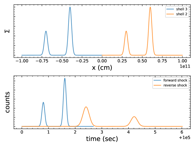
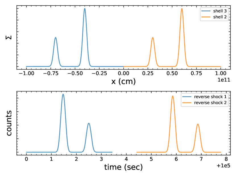
Figure 7: Simulated light curve with two situation. The upper panel in each figure represents the areal density distribution of shell 2 and shell 3, the peaks represents high-density area or blocks. The left panel shows shell 2 and shell 3 collision, and the right panel simulates shell 2, shell 3 collision with shell 1 in turn.

6 Conclusion and discussion

In this study, we firstly verified the result presented in Hakkila (2021) that the majority of GRB pulse light curves can be characterized by a smooth single-peaked component and a complex residual structure which is temporally symmetric. Our analysis utilized data from BATSE which replicated the previous results. Then we extended to the GBM data and got similar results. We found that the results obtained from the BATSE data showed a high ratio of success, with $85\%$ of the GRBs fitting the model well, which is in line with the findings in Hakkila (2021) where a ratio of $86.6\%$ was reported. When we applied the model to GBM 64 ms data, we obtained a lower ratio of $73.6\%$ and $77.1\%$, which could be attributed to the different effective areas between BATSE and GBM. This leads to varying signal-to-noise ratios that may impact the criteria of the model. Since the original model can only identify the symmetry of pulse orders but not the symmetry of pulse shapes, in order to further confirm this symmetry, we have designed a new model that can validate the symmetry of pulse shapes. However, our comparison between the translational model and the symmetrical model did not yield strong evidence to suggest that the symmetrical model is better. The calculated value of $\rm CCF_{Band}$ was almost the same between the two models. As shown in Figure 5, about half can be considered symmetrical and another half can be considered as translational. Both features could come from the structure of the ejected shells, i.e., the fast component represents the structure. We assume there are two shells with similar structure, if they collide each other, the fast component is symmetrical, while if they collide to the external shocked shell one by one, the fast component is translational. We suggest the future full SKA could be able to test this scenario because of its large field of view as well as high sensitivity. The Five-hundred-meter Aperture Spherical radio Telescope (FAST) also has a very high sensitivity (Nan et al., 2011). However, the small field of view makes the detection rate very low for the prompt radio emission.

We noticed that in the original model, the uncertainty of parameter $s_{mirror}$ is the main criterion rather than the value of CCF. We decided to abandon this approach as the uncertainty in the three-parameter model would increase, rendering the original criterion invalid. We also notice that the CCF value of different GRBs cannot be used for direct comparison, for the GRBs with bright residual usually show a larger CCF value. However, within our model, it is feasible to compare the translational and symmetrical models for a same GRB light curve without such concerns.

It is worth mentioning that, relative to the new method for identifying monotonic components, the original method just introduces a systematic deviation with convex shape, resulting in residuals with a concave systematic deviation. This is the reason why the residuals obtained by direct fitting show components that are obviously less than zero in the pulse duration window but near zero outside of the window. This deviation favors the symmetrical model but is against the translational model, which is the main reason why we developed the new approach to subtract the monotonic component.

Notice that the distribution of ${\rm CCF}_{sm}-{\rm CCF}_{tm}$ concentrates around 0. Therefore, only a small part of the fast component light curves should be determinately classified as symmetrical or translational. At present, it remains challenging to definitively categorize GRBs into distinct groups of translation and symmetry. We expect more light curves from various GRB telescopes could be considered in the further investigation.

We thank Weihua Lei, Yu Liu, Zipei Zhu and Kai Wang for helpful discussions. This work is in part supported by the National Key R&D Program of China (2022SKA0130100), and by the National Natural Science Foundation of China (Grant Nos. 12041306 and U1931203). We also acknowledge the science research grants from the China Manned Space Project with No. CMS-CSST-2021-B11. The computation is completed in the HPC Platform of Huazhong University of Science and Technology.

Table 2: Temporally symmetric model applies to BATSE dataset

Pulse	$B_{0}$	$BS$	$A$	$t_{s}$	$\tau_{1}$	$\tau_{2}$	$t_{0}$	$\sigma$	CCF	$R$	$p$	$t_{mirror}$	$\sigma_{t,mirror}$	$s_{mirror}$	$\sigma_{s,mirror}$
105	619.9	0.209	2763.0	1.93	10.75	0.26	…	…	0.812	5.97	0.00	4.16	0.27	0.19	0.14
107	547.1	0.023	37.0	…	…	…	-150.29	41.97	0.446	0.45	1.00	-186.94	23.38	0.88	0.41
109	643.3	0.087	540.8	-0.28	4.37	36.98	…	…	0.575	4.40	0.00	49.40	0.23	0.70	0.01
111	541.3	0.003	86.5	-16.83	16.15	26.5	…	…	0.180	1.04	0.42	1.08	20.49	0.21	0.56
114	550.0	-0.082	118.2	…	…	…	-0.43	2.25	0.582	1.45	0.00	-0.11	0.85	2.37	0.77
121	480.5	0.079	115.4	…	…	…	30.22	35.29	0.654	2.23	0.00	23.70	3.44	0.61	0.23
130	474.9	-0.106	316.9	…	…	…	30.3	24.15	0.678	5.24	0.00	27.04	0.11	1.07	0.01
160	587.8	0.004	239.3	…	…	…	11.43	5.53	0.595	4.65	0.00	14.21	1.51	0.84	0.39
171	546.1	0.007	56.5	…	…	…	7.4	8.81	0.370	1.11	0.00	8.18	4.42	1.09	0.50
179	532.6	-0.015	1050.8	…	…	…	1.89	0.23	0.746	4.97	0.00	1.71	0.11	1.57	0.55
214	595.0	0.013	45.1	…	…	…	10.91	13.27	0.602	1.38	0.00	5.20	0.26	0.77	0.06
218	551.5	-0.089	193.6	-1.12	1.57	0.33	…	…	0.774	1.95	0.00	0.42	0.20	0.34	0.46
222	583.4	-0.280	…	…	…	…	…	…	0.544	3.24	0.00	59.65	16.32	0.23	0.03
223	540.2	-0.052	84.9	-117.87	2090161.64	0.01	…	…	0.585	1.08	0.12	0.15	0.47	1.04	0.50
226	451.2	0.146	199.2	-30.05	129.41	27.59	…	…	0.533	2.36	0.00	23.11	18.99	0.31	0.03
228	600.5	0.000	217.0	-0.78	0.94	0.7	…	…	0.700	1.09	0.23	0.83	0.54	1.63	0.54
237	770.6	-0.094	167.6	-8.74	301.38	0.26	…	…	0.533	1.49	0.00	-0.06	0.81	0.65	0.46
249	1124.9	-0.251	7869.7	-5.78	729.09	1.03	…	…	0.741	43.21	0.00	21.68	0.02	0.72	0.01
257	485.0	0.012	388.9	-0.19	0.0	19.16	…	…	0.379	1.48	0.00	7.39	2.22	2.31	0.68
269	858.1	-2.324	318.2	-0.42	0.18	1.58	…	…	0.518	1.26	0.00	0.13	1.17	0.25	0.63
288	555.5	-0.048	56.0	…	…	…	5.28	7.18	0.397	1.08	0.05	-0.28	3.01	1.38	0.41
332	503.1	-0.016	266.8	-1.4	1.97	9.23	…	…	0.296	1.17	0.01	14.18	6.74	0.40	0.61
351	518.5	-0.107	149.5	…	…	…	49.35	23.37	0.680	2.02	0.00	41.01	0.24	1.36	0.07
394	500.0	-0.173	635.9	-22.36	317.03	5.85	…	…	0.676	5.00	0.00	22.98	0.08	0.63	0.01
398	620.4	-0.205	237.5	-3.65	2.17	7.6	…	…	0.462	1.75	0.00	-1.58	3.86	0.11	0.85
401	586.4	0.051	59.0	-2.39	1.05	1.69	…	…	0.507	1.09	0.08	0.09	1.32	0.69	0.62
408	525.8	0.076	78.4	…	…	…	41.09	30.68	0.438	1.88	0.00	28.63	1.64	1.10	0.22
414	522.1	-0.063	196.5	…	…	…	-1.07	0.43	0.723	1.61	0.00	-1.39	0.24	1.36	0.59
451	543.3	0.051	1766.8	2.35	8.59	1.04	…	…	0.706	5.67	0.00	4.44	0.49	0.28	0.09
465	468.6	0.037	43.9	…	…	…	-0.66	1.89	0.479	0.91	0.94	3.00	1.59	1.19	0.54
467	500.2	0.036	1199.1	-0.0	0.0	1.64	…	…	0.787	9.63	0.00	0.17	0.31	0.11	0.21
469	791.8	0.111	1023.8	1.76	0.27	2.06	…	…	0.662	3.16	0.00	2.57	0.27	0.49	0.22
472	467.7	0.022	17.8	…	…	…	7.21	30.23	0.329	0.93	1.00	-0.61	7.60	0.89	0.24
473	551.5	0.012	70.5	-1.96	0.15	13.41	…	…	0.243	1.06	0.08	5.25	8.34	1.21	0.55
493	484.8	0.113	246.7	-2.02	12.51	0.54	…	…	0.649	1.22	0.05	1.97	0.64	0.94	0.42
501	471.9	-0.064	198.0	-0.86	0.31	2.59	…	…	0.546	1.26	0.00	1.67	1.56	1.91	0.62
508	1030.2	-0.133	234.8	-5.89	916.63	0.03	…	…	0.786	1.10	0.08	-0.83	0.28	0.51	0.49
516	474.3	-0.130	168.3	…	…	…	0.99	2.34	0.493	1.22	0.01	0.07	1.42	0.36	0.53
526	509.1	0.000	80.6	…	…	…	-0.01	0.44	0.708	0.95	0.51	0.38	0.56	0.54	0.54
537	509.2	-0.099	277.9	-0.23	0.1	1.24	…	…	0.704	1.80	0.00	0.75	0.33	0.24	0.48
540	1004.0	0.038	324.6	-0.71	0.25	0.94	…	…	0.583	1.43	0.00	0.97	0.59	0.76	0.46
543	569.9	-0.001	1957.7	-0.21	0.36	1.73	…	…	0.810	9.57	0.00	2.17	0.01	0.66	0.03
548	542.3	0.043	306.5	-1.64	2.29	13.58	…	…	0.647	2.13	0.00	9.15	0.16	0.55	0.03
563	757.8	-0.126	394.3	-0.75	0.51	8.5	…	…	0.358	1.33	0.00	11.80	2.34	1.75	0.56
577	628.8	-0.002	135.4	-3.63	5.4	8.55	…	…	0.206	1.06	0.25	6.86	7.65	1.19	0.54
591	676.4	0.025	44.1	…	…	…	20.25	20.72	0.620	1.52	0.00	12.86	1.56	0.60	0.17
593	545.4	-0.050	…	…	…	…	…	…	0.375	1.02	0.04	5.86	0.74	2.12	0.44
594	537.5	-0.017	122.6	…	…	…	11.1	9.71	0.495	2.28	0.00	17.20	3.88	2.24	0.70
606	554.4	0.008	191.6	-1.45	1.18	7.54	…	…	0.537	1.43	0.00	4.51	0.55	1.02	0.26
612	566.3	-0.009	520.9	…	…	…	8.12	2.61	0.583	3.07	0.00	7.94	0.96	0.89	0.35
630	562.3	0.009	63.1	-20.06	134.97	2.5	…	…	0.298	0.90	1.00	4.62	3.62	0.69	0.48
647	536.4	-0.102	732.0	-0.48	0.83	13.99	…	…	0.876	4.70	0.00	6.84	0.09	0.46	0.02
658	428.5	0.123	207.1	-3.97	4.07	3.97	…	…	0.498	1.42	0.00	2.50	1.60	0.72	0.38
659	516.4	-0.047	191.9	-7.07	13.31	26.98	…	…	0.468	1.43	0.00	21.49	3.18	0.69	0.14
660	503.0	0.239	459.3	-0.63	0.93	4.2	…	…	0.800	6.72	0.00	3.56	0.48	0.68	0.18
666	612.1	-0.174	191.0	…	…	…	2.64	0.75	0.745	3.74	0.00	2.98	0.44	0.47	0.21
673	494.5	0.096	48.3	-41.99	756.87	3.16	…	…	0.234	0.89	1.00	19.32	7.51	1.04	0.53
676	587.3	-0.037	715.1	…	…	…	54.63	8.11	0.770	5.97	0.00	54.76	0.08	0.82	0.04
678	532.4	0.205	1563.9	-0.03	0.06	13.66	…	…	0.561	13.40	0.00	9.64	0.58	1.93	0.33
680	722.4	-0.041	194.6	-8.56	149.6	0.68	…	…	0.478	1.22	0.00	0.17	1.24	2.30	0.58
685	540.8	0.039	64.6	-6.17	9.11	3.8	…	…	0.587	1.41	0.00	-0.14	0.29	0.28	0.16
686	616.5	-0.016	137.1	-0.73	0.05	5.42	…	…	0.480	1.23	0.00	2.06	2.18	0.57	0.66
690	522.9	0.061	40.2	…	…	…	0.92	1.36	0.672	1.43	0.00	0.68	0.59	0.95	0.33
692	768.4	0.180	…	…	…	…	…	…	0.578	1.26	0.00	3.93	0.00	1.96	0.12
704	588.3	-0.260	152.4	-0.38	0.0	17.09	…	…	0.462	1.66	0.00	0.19	4.29	0.33	0.88
711	745.4	-0.467	398.9	-1.33	9.91	0.19	…	…	0.669	1.34	0.01	0.06	0.25	1.56	0.53
727	844.7	-0.010	218.8	-4.01	34.6	0.59	…	…	0.512	1.03	0.43	2.43	1.09	1.91	0.47
734	522.0	0.008	204.7	-1.91	74.58	0.05	…	…	0.821	1.05	0.16	0.04	0.17	1.03	0.52
741	553.1	0.029	51.1	-5.61	4.8	3.69	…	…	0.303	0.98	0.74	3.32	2.81	0.99	0.47
752	564.6	-0.050	195.1	…	…	…	0.94	0.88	0.725	1.26	0.01	0.08	0.67	0.12	0.31
753	774.2	0.305	112.7	-116.95	189458.41	0.07	…	…	0.475	1.13	0.03	2.15	57.36	1.22	0.55
755	540.4	-0.054	156.5	-0.43	0.1	1.41	…	…	0.723	2.31	0.00	0.32	0.41	0.48	0.53
761	546.3	-0.047	301.3	-0.79	0.3	39.72	…	…	0.699	4.38	0.00	20.85	0.93	0.58	0.05
764	429.2	0.046	138.1	-7.4	13.54	5.28	…	…	0.367	1.13	0.05	-3.02	6.04	0.44	0.74
795	480.4	-0.035	172.8	-1.63	1.78	7.32	…	…	0.419	1.32	0.00	2.25	1.40	0.26	0.42
803	532.6	0.143	155.1	…	…	…	2.86	2.86	0.699	2.27	0.00	0.95	0.52	1.11	0.16
815	488.4	-0.052	89.1	…	…	…	-1.32	6.74	0.463	0.98	0.98	0.59	1.95	0.52	0.32
816	617.4	-0.030	…	…	…	…	…	…	0.574	1.22	0.00	12.16	0.61	2.43	0.16
820	527.2	-0.030	49.3	…	…	…	8.04	11.32	0.325	1.11	0.00	0.10	6.74	0.22	0.62
824	788.3	0.059	129.2	-4.3	6.95	13.62	…	…	0.206	1.13	0.00	27.43	12.92	0.68	0.61
829	708.5	-0.000	1274.3	-3.17	14.86	3.45	…	…	0.689	3.03	0.00	4.40	0.53	0.42	0.15
840	764.1	-0.018	193.3	…	…	…	2.53	2.33	0.575	3.09	0.00	2.04	0.91	1.54	0.39
845	530.1	0.051	187.8	-120.83	4030435.2	0.0	…	…	0.653	2.29	0.00	0.33	0.27	0.18	0.58
869	580.8	-0.060	…	…	…	…	…	…	0.756	3.22	0.00	104.37	0.00	1.72	0.02
914	499.9	0.200	442.5	-0.84	1.43	1.3	…	…	0.644	1.37	0.01	0.59	0.77	0.51	0.60
927	782.2	-0.004	113.7	-1.89	0.62	4.24	…	…	0.468	1.22	0.00	1.76	2.04	1.74	0.56
942	510.3	-0.112	66.4	…	…	…	1.06	1.71	0.484	1.14	0.02	3.07	1.22	1.39	0.59
973	516.6	-0.140	1243.0	-0.36	0.75	7.75	…	…	0.876	11.71	0.00	23.16	0.14	0.11	0.17
974	575.5	-0.040	55.4	…	…	…	-0.05	1.04	0.593	1.13	0.04	0.48	0.99	0.46	0.64
1008	546.6	-0.008	1080.6	-121.85	44305.35	0.38	…	…	0.807	8.34	0.00	8.34	0.21	0.86	0.07
1009	502.7	0.093	56.5	…	…	…	91.01	21.46	0.465	1.55	0.00	93.38	0.42	0.72	0.04
1025	941.9	-1.705	2491.7	…	…	…	2.02	0.35	0.874	10.45	0.00	1.75	0.02	0.88	0.66
1036	871.5	-0.140	97.2	-121.86	3870.0	4.46	…	…	0.307	1.27	0.00	25.60	9.26	0.56	0.48
1039	549.1	-0.035	241.3	-5.95	45.8	2.31	…	…	0.458	1.29	0.00	1.83	2.23	0.79	0.28
1042	526.6	0.149	58.4	…	…	…	-4.83	10.18	0.609	1.95	0.00	0.08	1.43	0.28	0.09
1046	486.3	-0.053	134.1	…	…	…	1.5	3.94	0.555	1.24	0.00	4.84	1.83	1.07	0.27
1085	610.0	-0.152	4809.9	-4.96	41.43	2.46	…	…	0.807	17.58	0.00	3.71	0.23	0.90	0.06
1087	426.0	0.209	117.2	…	…	…	-120.55	289.83	0.124	0.94	1.00	1.99	59.93	1.26	0.59
1110	530.8	0.020	80.7	-4.2	12.43	4.02	…	…	0.272	0.99	0.78	14.15	4.84	0.78	0.46
1114	527.1	-0.076	451.1	-120.38	520921.5	0.03	…	…	0.665	7.02	0.00	2.64	0.37	0.88	0.32
1122	733.6	-0.029	1622.8	-121.86	63155.52	0.27	…	…	0.607	20.33	0.00	10.17	0.63	1.72	0.57
1123	554.5	0.157	34.0	-1.37	0.0	444.27	…	…	0.223	0.91	1.00	-0.24	18.46	0.86	0.62
1125	797.9	0.071	90.7	-2.32	1.39	5.42	…	…	0.266	1.03	0.33	12.74	4.97	1.63	0.53
1126	687.1	-0.021	130.9	-0.82	0.14	6.91	…	…	0.335	1.13	0.00	17.74	3.87	0.96	0.64
1141	494.3	-0.002	1653.7	-13.79	188.69	2.14	…	…	0.656	10.53	0.00	8.65	0.09	0.60	0.04
1148	468.1	0.043	167.2	-1.03	0.92	14.62	…	…	0.319	1.87	0.00	13.52	6.16	2.06	0.77
1150	516.5	-0.016	144.3	…	…	…	44.64	9.12	0.640	2.33	0.00	43.86	0.46	2.26	0.34
1152	566.5	-0.067	45.6	-10.98	19.11	6.27	…	…	0.217	0.95	0.96	16.86	6.53	0.91	0.52
1153	541.2	-0.052	63.5	-3.28	7.66	1.3	…	…	0.462	0.95	0.78	2.09	1.43	0.79	0.48
1156	522.2	-0.018	92.9	…	…	…	59.1	41.45	0.295	1.23	0.00	49.38	9.39	1.11	0.35
1159	888.1	-0.154	714.1	-2.32	25.38	0.35	…	…	0.665	2.30	0.00	0.59	0.27	1.67	0.51
1167	548.1	-0.037	65.8	-1.44	0.32	4.47	…	…	0.338	1.13	0.01	9.72	3.18	1.87	0.58
1190	489.0	0.036	447.9	…	…	…	0.98	1.12	0.799	6.15	0.00	1.39	0.05	0.72	0.38
1192	549.0	-0.214	23.3	…	…	…	24.1	18.81	0.345	1.19	0.00	2.58	10.46	0.10	0.68
1197	574.3	-0.077	166.7	…	…	…	6.97	5.84	0.514	1.77	0.00	7.91	2.49	0.27	0.59
1200	547.5	-0.027	249.4	-10.58	94.59	2.57	…	…	0.346	1.24	0.00	-0.19	3.27	0.10	0.53
1213	530.1	-0.033	35.6	…	…	…	8.28	7.51	0.356	1.15	0.00	20.17	4.59	1.98	0.70
1218	479.6	0.033	209.2	…	…	…	3.96	2.78	0.540	1.41	0.00	1.21	1.04	1.17	0.35
1221	559.5	-0.173	196.7	-0.69	0.63	1.67	…	…	0.516	1.13	0.13	0.09	1.20	1.33	0.48
1279	573.6	-0.224	90.6	…	…	…	6.25	9.1	0.452	1.38	0.00	5.94	2.26	1.62	0.56
1288	545.3	0.011	327.5	1.58	0.41	94.66	…	…	0.583	6.02	0.00	67.20	2.71	0.80	0.72
1291	521.1	0.008	167.3	-1.93	1.71	6.1	…	…	0.570	3.45	0.00	0.69	0.53	0.25	0.09
1301	553.6	0.127	44.0	-50.86	2076.74	1.23	…	…	0.314	0.84	1.00	9.51	4.03	0.68	0.50
1303	710.1	0.031	148.9	-14.64	124.91	2.98	…	…	0.485	2.59	0.00	3.76	2.36	0.46	0.66
1306	823.9	-0.165	109.0	-6.51	35.74	1.29	…	…	0.428	1.08	0.12	3.19	1.60	1.75	0.52
1321	608.2	-0.262	141.6	-121.86	134.87	66.67	…	…	0.620	2.46	0.00	-37.36	1.67	0.81	0.06
1328	605.2	-0.170	64.5	…	…	…	-24.64	43.43	0.618	1.49	0.00	-20.48	1.62	1.43	0.23
1346	1128.1	-0.091	153.5	…	…	…	1.0	1.07	0.677	3.22	0.00	1.32	0.45	2.36	0.66
1365	548.9	-0.037	56.2	-120.65	74069.36	1.14	…	…	0.489	2.11	0.00	181.28	5.41	0.58	0.22
1379	491.4	-0.092	240.0	-0.96	1.06	0.57	…	…	0.767	1.71	0.00	0.17	0.38	0.52	0.31
1382	512.5	-0.039	76.6	-5.17	12.35	1.46	…	…	0.498	1.09	0.10	1.64	1.54	0.63	0.44
1385	499.4	-0.088	660.2	3.47	9.15	11.08	…	…	0.561	4.39	0.00	25.05	4.24	2.16	0.86
1388	583.7	0.148	292.7	-57.3	109797.12	0.03	…	…	0.722	1.51	0.00	0.04	0.42	1.17	0.35
1390	527.8	0.037	54.6	-4.89	2.15	7.94	…	…	0.233	0.97	0.91	17.61	6.05	1.85	0.47
1396	608.9	-0.020	85.2	…	…	…	9.69	10.42	0.558	2.09	0.00	13.93	0.54	2.32	0.21
1406	482.5	-0.053	434.3	-1.44	2.57	7.24	…	…	0.318	1.34	0.00	10.45	3.51	0.45	0.66
1413	498.6	-0.066	107.4	-121.15	17469.69	0.78	…	…	0.539	1.59	0.00	-1.22	3.54	0.56	0.74
1416	471.3	0.016	205.8	…	…	…	0.69	0.99	0.854	4.44	0.00	1.05	0.04	1.68	0.22
1419	540.7	-0.306	935.4	107.27	30.44	3.95	…	…	0.707	2.96	0.00	118.69	0.10	0.97	0.08
1425	422.2	-0.083	912.1	…	…	…	4.66	2.55	0.854	15.91	0.00	4.08	0.02	0.38	0.01
1432	783.5	-0.155	96.7	-21.21	49.03	10.72	…	…	0.231	0.99	0.93	15.10	12.49	2.37	0.58
1435	510.8	-0.020	70.4	-120.83	5110000.0	0.0	…	…	0.669	1.10	0.08	-0.98	0.35	0.88	0.63
1440	758.7	-0.032	1740.8	…	…	…	15.57	1.79	0.598	24.30	0.00	16.23	0.79	1.38	0.59
1443	484.1	0.139	851.6	-0.17	0.12	0.89	…	…	0.810	5.41	0.00	1.62	0.02	0.41	0.05
1446	551.7	0.073	91.5	-56.75	3079.85	1.23	…	…	0.247	0.97	0.98	6.06	5.64	1.23	0.60
1447	997.7	0.178	425.4	-0.76	0.55	11.77	…	…	0.678	1.89	0.00	1.64	0.13	0.26	0.03
1449	484.0	-0.042	136.1	-0.92	0.82	11.41	…	…	0.517	2.36	0.00	8.96	2.84	0.29	0.14
1452	1267.4	0.287	172.5	-1.45	0.4	5.34	…	…	0.401	1.23	0.00	7.52	3.12	0.50	0.73
1456	623.1	-0.199	83.3	-6.0	3.29	8.17	…	…	0.287	1.00	0.71	8.34	6.62	0.60	0.54
1459	510.3	-0.036	65.6	…	…	…	29.8	18.85	0.430	1.25	0.00	18.46	8.37	0.72	0.19
1465	499.6	-0.177	41.5	-4.19	1.38	4.54	…	…	0.317	1.00	0.56	10.49	4.68	2.05	0.53
1466	501.4	0.049	230.5	-50.36	3288.05	0.85	…	…	0.627	1.96	0.00	-0.47	0.55	2.19	0.47
1467	529.1	-0.100	469.4	-1.33	8.9	3.55	…	…	0.445	1.47	0.00	3.74	3.08	0.25	0.37
1533	536.0	0.066	116.9	…	…	…	25.03	26.73	0.480	4.62	0.00	37.22	3.97	0.47	0.83
1540	503.8	0.025	73.4	…	…	…	21.73	11.71	0.535	1.67	0.00	17.55	3.30	1.28	0.20
1551	835.7	0.072	93.6	-2.16	0.1	13.62	…	…	0.277	1.24	0.00	18.26	7.50	1.74	0.67
1552	532.6	0.006	54.9	-6.81	5.41	14.17	…	…	0.194	0.98	0.95	38.60	12.79	2.41	0.50
1553	770.8	0.215	2797.2	…	…	…	0.48	0.3	0.900	24.52	0.00	0.46	0.00	0.99	0.03
1558	488.1	-0.091	62.8	-4.28	3.55	4.64	…	…	0.336	0.97	0.87	5.37	4.67	0.56	0.49
1559	481.4	-0.023	139.3	-2.51	2.17	12.4	…	…	0.201	1.10	0.06	13.24	10.93	1.00	0.56
1561	623.9	-0.252	127.3	-1.68	1.3	8.97	…	…	0.270	1.12	0.00	18.26	5.94	1.45	0.63
1567	483.2	0.131	117.8	-11.91	133.11	1.75	…	…	0.401	1.28	0.00	5.38	1.94	0.85	0.50
1574	505.2	-0.058	62.3	-9.87	4.18	31.12	…	…	0.298	1.50	0.00	71.92	18.40	0.40	0.76
1578	511.1	-0.038	626.4	-28.99	1307.98	1.01	…	…	0.829	3.65	0.00	3.90	0.05	2.03	0.13
1579	508.1	0.005	543.4	1.18	3.57	1.17	…	…	0.689	7.70	0.00	4.56	0.19	2.19	0.19
1580	520.3	-0.061	207.9	-0.42	0.1	5.91	…	…	0.469	1.32	0.00	0.48	2.33	0.27	0.56
1586	461.1	0.050	50.7	…	…	…	29.86	42.62	0.600	1.42	0.00	7.31	0.66	1.07	0.25
1590	473.7	0.110	72.8	…	…	…	13.2	20.17	0.412	1.12	0.00	11.48	2.26	2.47	0.43
1601	931.1	0.154	334.1	-4.78	19.26	4.09	…	…	0.726	4.92	0.00	5.42	0.04	1.18	0.02
1604	478.0	0.009	80.6	-3.27	3.14	4.56	…	…	0.392	1.04	0.39	6.19	4.15	0.45	0.65
1614	621.2	-0.119	91.0	-3.2	2.07	18.93	…	…	0.431	1.51	0.00	18.59	4.25	1.79	0.56
1623	588.0	-0.000	183.5	…	…	…	24.91	18.47	0.489	3.79	0.00	0.16	2.58	0.14	0.69
1625	499.5	0.035	3277.1	4.22	0.0	9.43	…	…	0.852	45.76	0.00	7.92	0.04	0.61	0.01
1628	533.2	-0.060	117.7	…	…	…	14.7	16.78	0.595	2.21	0.00	17.78	1.59	1.27	0.17
1642	589.1	-0.041	67.5	-5.52	2.24	30.51	…	…	0.132	1.04	0.18	36.98	29.55	1.23	0.62
1646	574.9	-0.054	26.4	…	…	…	51.44	95.85	0.217	0.93	1.00	10.12	26.43	0.10	0.75
1651	453.2	0.050	566.5	-0.16	0.07	2.06	…	…	0.807	2.30	0.00	1.83	0.59	0.34	0.15
1652	564.9	-0.039	670.7	…	…	…	50.36	7.27	0.675	3.38	0.00	49.89	0.64	0.76	0.14
1653	549.5	-0.002	68.9	-7.96	3.63	16.44	…	…	0.411	1.38	0.00	8.81	5.52	0.59	0.54
1655	602.1	0.223	61.4	-11.37	15.33	14.46	…	…	0.173	1.01	0.67	31.05	15.34	2.27	0.55
1657	492.3	-0.033	69.9	-18.1	360.22	1.17	…	…	0.370	0.95	0.95	7.89	3.01	1.36	0.49
1660	553.9	-0.047	60.5	…	…	…	14.13	15.64	0.550	2.28	0.00	0.45	9.89	0.52	0.55
1661	526.2	-0.042	61.8	-1.86	1.55	10.81	…	…	0.213	1.02	0.43	5.57	7.63	1.62	0.55
1663	768.1	-0.036	2913.5	-52.18	2492.2	1.53	…	…	0.681	26.92	0.00	16.08	0.05	0.51	0.03
1664	499.2	-0.080	1491.7	-120.58	2000000.0	0.01	…	…	0.705	15.63	0.00	2.12	0.09	0.62	0.45
1667	549.7	-0.015	517.0	…	…	…	51.58	4.45	0.781	3.79	0.00	49.89	0.15	1.28	0.18
1676	522.7	0.044	490.6	…	…	…	25.75	18.57	0.605	16.44	0.00	26.87	0.90	0.85	0.06
1679	462.7	-0.000	110.2	-4.61	59.98	0.34	…	…	0.533	1.15	0.07	1.14	0.64	1.51	0.55
1683	509.2	0.009	1293.0	…	…	…	1.86	1.06	0.691	9.82	0.00	2.31	0.05	0.49	0.09
1687	525.2	0.042	44.4	-8.65	5.81	8.23	…	…	0.266	0.94	0.99	13.39	6.17	0.86	0.53
1693	523.9	0.015	68.6	-2.66	3.08	2.99	…	…	0.331	1.04	0.31	2.97	2.79	1.47	0.53
1700	552.8	0.089	221.3	-0.68	0.87	2.1	…	…	0.453	1.17	0.04	1.43	1.23	1.27	0.49
1709	717.3	-0.003	2505.9	-9.45	521.76	0.23	…	…	0.907	15.10	0.00	1.48	0.01	1.09	0.04
1711	899.7	0.346	1406.5	…	…	…	3.39	3.09	0.936	36.38	0.00	3.05	0.03	0.94	0.02
1714	627.1	0.007	37.6	-3.9	0.08	82.05	…	…	0.128	1.05	0.00	4.95	48.66	0.79	0.56
1717	538.8	0.053	539.2	-46.49	16899.19	0.15	…	…	0.671	2.04	0.00	3.28	0.55	0.51	0.35
1723	520.5	-0.020	57.0	-7.57	8.7	11.33	…	…	0.194	1.03	0.37	32.04	12.62	0.82	0.61
1730	546.8	-0.075	70.4	-3.93	2.22	14.98	…	…	0.325	1.14	0.00	3.06	4.63	0.39	0.40
1733	858.3	-0.193	677.6	-0.93	7.3	2.56	…	…	0.607	2.13	0.00	1.50	0.83	0.44	0.12
1734	513.1	-0.025	219.9	…	…	…	3.72	1.31	0.628	3.13	0.00	2.58	0.73	0.77	0.65
1806	503.2	0.085	61.9	-5.43	5.18	8.14	…	…	0.279	1.17	0.00	1.58	6.97	0.25	0.63
1807	505.4	0.058	244.5	-0.42	0.06	33.44	…	…	0.625	1.83	0.00	5.83	0.47	0.16	0.02
1883	536.7	-0.051	1028.2	-0.53	1.47	1.94	…	…	0.537	1.61	0.00	3.79	1.33	0.68	0.69
1885	504.8	0.022	108.4	-3.98	2.13	21.48	…	…	0.175	1.03	0.56	40.59	18.75	1.45	0.56
1922	435.8	0.133	333.0	…	…	…	2.86	1.19	0.826	6.92	0.00	2.69	0.13	0.75	0.10
1924	530.4	0.010	186.4	-9.24	79.07	1.21	…	…	0.494	1.21	0.01	0.65	1.50	0.60	0.36
1956	508.3	-0.046	556.7	-2.87	19.24	1.73	…	…	0.570	1.92	0.00	1.00	1.04	0.61	0.27
1967	535.7	-0.072	286.3	4.55	1.16	8.05	…	…	0.563	1.64	0.00	11.27	1.79	0.34	0.21
1974	657.8	-0.210	1267.3	-121.86	128551.62	0.12	…	…	0.840	9.15	0.00	3.32	0.42	0.71	0.10
1982	508.2	-0.024	217.3	…	…	…	13.5	10.37	0.688	1.98	0.00	16.15	0.16	1.00	0.05
1989	600.4	-0.188	…	…	…	…	…	…	0.745	5.52	0.00	146.53	1.06	0.26	0.01
1991	594.8	0.225	157.4	…	…	…	-0.04	0.24	0.717	0.83	0.66	-0.05	1.92	0.88	0.42
1993	1168.8	-0.022	267.5	-0.45	0.0	14.51	…	…	0.712	2.53	0.00	5.50	0.56	0.26	0.13
2018	536.5	0.057	235.0	…	…	…	7.23	4.72	0.586	1.54	0.00	5.78	0.55	1.24	0.25
2019	589.9	-0.269	197.0	-1.08	0.93	12.29	…	…	0.516	1.65	0.00	2.69	2.22	0.12	0.72
2041	504.3	-0.013	226.6	-121.86	1114054.97	0.01	…	…	0.903	5.78	0.00	0.80	0.32	0.87	0.65
2044	1064.1	-0.110	171.0	-120.83	1500000.0	0.01	…	…	0.603	1.34	0.00	0.13	0.46	0.45	0.48
2047	610.8	0.238	62.6	…	…	…	13.62	8.55	0.703	2.72	0.00	11.84	2.34	0.75	0.34
2061	543.4	-0.095	198.6	-11.42	23.45	48.51	…	…	0.534	2.08	0.00	58.06	1.13	0.84	0.06
2067	490.0	-0.091	3308.3	…	…	…	18.8	4.14	0.755	10.14	0.00	18.87	1.42	1.00	0.13
2090	498.9	-0.070	…	…	…	…	…	…	0.793	7.80	0.00	3.04	0.00	1.90	0.01
2798	621.7	0.061	4005.7	-1.4	93.51	2.64	…	…	0.689	13.38	0.00	15.13	0.11	1.38	0.15
3003	509.6	0.089	499.9	-1.37	23.98	5.16	…	…	0.502	1.68	0.00	9.33	2.89	0.43	0.34
3040	577.3	-0.075	286.9	-0.38	0.18	5.36	…	…	0.512	1.58	0.00	4.70	2.88	0.35	0.43
5614	671.6	-0.064	29850.8	7.24	0.72	1.72	…	…	0.846	47.45	0.00	8.90	0.02	0.30	0.01
6581	892.0	-0.046	7263.7	45.65	20.65	0.19	…	…	0.868	25.89	0.00	47.62	0.00	0.56	0.01

Table 2: Continued

Table 3: Temporally symmetric model applies to GBM dataset

Trigger	$B_{0}$	$BS$	$A$	$t_{s}$	$\tau_{1}$	$\tau_{2}$	$t_{0}$	$\sigma$	CCF	$R$	$p$	$t_{mirror}$	$\sigma_{t,mirror}$	$s_{mirror}$	$\sigma_{s,mirror}$
bn200101861	150.9	-0.002	1388.7	…	…	…	11.9	0.77	0.653	9.00	0.00	11.65	0.11	2.49	0.48
bn200103689	146.0	0.017	7.9	-9.14	0.46	165.16	…	…	0.071	1.04	0.00	136.79	108.88	1.80	0.32
bn200111633	283.6	-0.016	331.3	3.24	49.38	0.09	…	…	0.810	2.75	0.00	5.37	0.11	1.00	0.16
bn200125864	118.8	0.014	1005.1	0.95	0.21	2.53	…	…	0.748	18.24	0.00	2.19	0.05	0.25	0.02
bn200130417	134.2	0.020	516.1	-0.5	2.2	0.71	…	…	0.841	3.62	0.00	1.47	0.26	0.43	0.08
bn200219998	190.0	-0.051	306.4	-5.2	75.37	0.91	…	…	0.672	3.24	0.00	4.23	0.61	0.63	0.45
bn200227306	145.4	-0.022	91.6	-27.21	661.73	2.07	…	…	0.341	1.25	0.00	3.96	51.67	0.86	0.36
bn200228291	162.6	-0.016	279.1	-4.01	90.58	0.35	…	…	0.739	3.25	0.00	1.07	0.14	0.85	0.20
bn200306934	133.8	0.063	7.8	-135.04	57.44	28071.86	…	…	0.068	1.04	0.00	454.61	36.58	0.33	0.20
bn200313071	124.3	-0.045	606.8	-1.75	9.9	1.96	…	…	0.707	5.88	0.00	4.04	0.20	0.14	0.25
bn200317028	117.6	-0.019	143.7	-2.95	18.11	1.24	…	…	0.646	2.34	0.00	3.98	1.10	0.62	0.38
bn200323782	237.5	0.050	525.3	-1.93	33.79	0.2	…	…	0.831	2.54	0.00	0.72	0.16	2.08	0.42
bn200325620	145.1	0.003	52.1	-14.68	52.05	9.77	…	…	0.507	1.75	0.00	7.82	0.91	0.94	0.18
bn200402824	181.7	0.001	24.8	…	…	…	-84.95	87.41	0.406	1.25	0.00	-93.89	0.00	0.39	0.05
bn200412290	144.8	-0.021	279.3	-0.06	0.0	7.02	…	…	0.732	7.70	0.00	3.75	0.04	0.46	0.02
bn200412381	126.9	-0.040	1421.9	…	…	…	9.41	0.97	0.794	21.74	0.00	9.66	0.08	1.11	0.23
bn200421865	145.3	0.011	32.0	-31.54	168.62	15.56	…	…	0.194	1.11	0.00	20.97	14.88	1.01	0.39
bn200506208	146.2	-0.026	26.4	-1.16	0.01	1.18	…	…	0.621	1.20	0.01	1.01	38.10	1.31	0.40
bn200510445	156.2	-0.014	145.9	-0.64	0.81	2.75	…	…	0.670	2.61	0.00	1.62	0.47	0.19	0.18
bn200524211	147.5	-0.017	120.1	-6.36	49.01	2.79	…	…	0.543	2.18	0.00	2.02	1.09	0.52	0.34
bn200528436	111.0	-0.007	113.1	20.17	14.93	11.14	…	…	0.763	4.03	0.00	44.04	0.23	0.83	0.04
bn200529504	208.8	0.163	73.4	…	…	…	-2.36	115.49	0.072	6.07	0.00	-111.10	27.55	0.17	0.50
bn200530031	149.7	0.002	108.1	-34.16	696.99	3.19	…	…	0.411	2.58	0.00	16.37	17.32	0.79	0.56
bn200531119	149.1	0.008	24.2	…	…	…	7.78	6.53	0.460	1.24	0.00	4.65	1.76	1.72	0.37
bn200605762	296.8	-0.022	1350.8	-0.06	0.0	0.17	…	…	0.894	4.44	0.00	0.24	0.04	0.73	0.60
bn200613229	143.1	0.043	215.1	-29.88	744.76	2.38	…	…	0.688	3.26	0.00	12.46	0.16	0.56	0.11
bn200623752	209.8	0.042	226.5	-0.06	0.0	0.16	…	…	0.896	2.64	0.00	0.15	25.88	0.38	0.60
bn200711461	282.1	-0.057	164.8	0.12	5.06	2.11	…	…	0.713	2.65	0.00	4.01	0.52	0.37	0.37
bn200716060	152.4	0.010	280.5	28.47	0.28	9.12	…	…	0.617	6.66	0.00	37.13	3.75	0.12	0.05
bn200716957	162.2	-0.036	399.1	0.13	0.0	1.39	…	…	0.943	12.14	0.00	1.11	0.12	0.67	0.17
bn200722094	260.2	-0.014	41.9	-12.9	25.26	34.26	…	…	0.687	1.84	0.00	30.45	21.86	0.52	0.24
bn200801352	337.2	-0.041	21.1	…	…	…	60.06	138.49	0.082	1.05	0.00	2.95	3.19	1.58	0.32
bn200801650	240.8	-0.032	55.4	-0.81	0.02	29.55	…	…	0.339	1.23	0.00	24.14	15.51	0.61	0.22
bn200803149	150.6	-0.037	73.8	…	…	…	102.61	10.42	0.552	2.60	0.00	104.80	1.21	1.30	0.56
bn200809255	166.0	-0.056	79.7	…	…	…	1.25	141.61	0.124	1.20	0.00	7.10	23.34	1.33	0.37
bn200826187	323.9	-0.057	1496.7	…	…	…	0.41	0.27	0.763	7.53	0.00	0.40	0.13	2.08	0.56
bn200826923	178.4	-0.014	1016.6	…	…	…	6.13	2.25	0.722	5.73	0.00	7.29	44.77	0.77	0.23
bn200829582	175.9	-0.019	1399.6	…	…	…	20.16	1.57	0.662	7.37	0.00	20.49	73.08	0.75	0.20
bn200908886	133.3	0.060	21.9	…	…	…	-131.97	191.32	0.074	1.77	0.00	61.16	1.29	0.47	0.10
bn200909168	161.1	0.018	53.5	-1.36	0.16	9.49	…	…	0.673	2.33	0.00	4.89	5.89	0.30	0.27
bn200914534	224.4	-0.101	68.2	-0.75	0.41	29.19	…	…	0.373	1.44	0.00	0.37	3.30	0.20	0.27
bn200919964	142.0	-0.014	92.8	0.25	8.37	15.71	…	…	0.746	2.87	0.00	26.49	0.62	0.46	0.04
bn200920831	150.4	-0.020	15.0	-137.79	372.68	308.56	…	…	0.121	2.42	0.00	229.62	42.92	1.85	0.58
bn201007123	159.2	0.001	205.5	…	…	…	128.89	0.64	0.718	2.12	0.00	129.07	50.13	1.87	0.57
bn201016019	239.1	-0.000	4655.0	5.08	6.3	0.69	…	…	0.768	14.32	0.00	7.37	0.18	0.43	0.09
bn201020732	255.2	-1.378	664.8	7.78	1.56	2.16	…	…	0.752	7.61	0.00	10.96	0.04	0.14	0.05
bn201104001	166.4	0.019	143.9	-0.13	0.0	4.47	…	…	0.599	2.53	0.00	2.18	0.53	1.73	0.23
bn201116035	231.3	-0.019	475.9	…	…	…	5.22	1.9	0.707	6.33	0.00	3.70	0.21	0.93	0.55
bn201208252	138.6	-0.016	49.3	…	…	…	12.0	3.73	0.517	1.42	0.00	12.14	1.63	0.55	0.38
bn201216963	140.0	-0.019	380.9	…	…	…	22.59	10.07	0.788	9.04	0.00	17.02	169.39	0.94	0.37
bn201218177	182.9	-0.039	473.1	…	…	…	8.79	4.28	0.672	9.13	0.00	6.43	126.01	1.49	0.47
bn201221963	23.3	-0.045	246.3	…	…	…	479.03	757.96	0.068	4.50	0.00	-88.28	0.04	0.25	0.70
bn201231550	172.3	-0.077	36.6	-1.7	0.1	27.67	…	…	0.591	1.45	0.00	4.83	0.48	0.42	0.10
bn210104477	141.1	0.001	46.9	…	…	…	25.31	5.55	0.668	2.88	0.00	22.89	1.26	0.63	0.16
bn210123305	137.3	-0.032	0.0	…	…	…	-133.2	36.31	0.157	1.15	0.00	-88.22	78.34	1.71	0.34
bn210306162	141.5	0.001	182.8	…	…	…	6.02	3.14	0.724	7.70	0.00	3.43	0.13	0.74	0.04
bn210323918	145.7	-0.004	269.7	…	…	…	0.07	0.08	0.993	2.75	0.00	0.09	40.30	1.00	0.47
bn210324833	127.9	-0.009	75.8	…	…	…	41.89	16.0	0.543	1.69	0.00	28.71	94.55	2.30	0.33
bn210406949	132.6	-0.019	272.1	-16.57	169.01	4.13	…	…	0.646	3.24	0.00	15.74	1.99	0.57	0.34
bn210410037	349.9	-0.074	416.0	-0.06	0.0	7.31	…	…	0.417	2.56	0.00	0.82	1.24	0.27	0.95
bn210411688	238.4	-0.056	65.6	-11.22	66.63	3.83	…	…	0.472	1.52	0.00	9.83	1.43	0.22	0.18
bn210422573	120.6	0.016	48.5	…	…	…	4.13	3.86	0.663	1.50	0.00	2.94	0.52	0.76	0.12
bn210511477	124.8	0.014	273.5	…	…	…	4.29	1.36	0.786	2.69	0.00	3.40	0.12	1.56	0.36
bn210518545	163.8	0.013	101.0	…	…	…	4.52	2.39	0.542	1.31	0.00	2.99	1.14	0.80	0.24
bn210524208	129.4	-0.014	236.2	…	…	…	12.47	3.22	0.779	6.19	0.00	12.99	73.02	0.87	0.34
bn210528586	328.4	0.038	552.5	-1.45	21.81	0.15	…	…	0.787	4.28	0.00	0.46	0.04	0.64	0.22
bn210529677	0.0	0.002	193.6	…	…	…	241.79	487.64	0.069	23.14	0.02	136.76	116.09	1.16	0.38
bn210531500	159.1	-0.045	483.9	-0.13	2.1	8.65	…	…	0.670	10.21	0.00	9.66	2.06	0.49	0.11
bn210606945	170.5	0.009	225.2	41.39	2.27	11.42	…	…	0.626	6.36	0.00	53.27	0.97	0.42	0.06
bn210610827	164.3	-0.017	188.6	…	…	…	35.11	11.6	0.738	2.94	0.00	28.97	0.32	1.08	0.27
bn210619532	155.5	-0.010	269.7	-0.21	0.24	0.43	…	…	0.764	2.70	0.00	0.29	0.22	0.48	0.28
bn210619999	463.9	-0.265	3875.1	-0.16	0.7	1.92	…	…	0.678	10.56	0.00	1.03	0.22	0.64	0.20
bn210627748	169.7	0.026	93.1	…	…	…	6.56	4.12	0.702	2.14	0.00	4.28	10.79	1.60	0.22
bn210704815	141.9	-0.018	986.7	-0.54	5.59	0.32	…	…	0.834	10.01	0.00	0.76	0.03	0.57	0.11
bn210706346	171.8	0.001	123.4	-7.61	195.82	0.44	…	…	0.616	1.43	0.00	1.05	0.78	0.78	0.32
bn210706571	145.1	-0.007	219.4	…	…	…	1.71	1.26	0.758	5.03	0.00	1.31	0.14	0.48	0.12
bn210714331	183.8	-0.031	453.2	0.4	0.51	6.08	…	…	0.647	2.60	0.00	2.30	0.39	0.25	0.06
bn210715866	247.5	-0.009	166.4	…	…	…	0.12	0.15	0.920	2.11	0.00	0.07	43.86	0.76	0.59
bn210725048	300.8	-0.011	104.6	…	…	…	2.99	2.06	0.678	2.28	0.00	3.03	0.41	0.92	0.28
bn210727410	233.8	0.013	127.9	…	…	…	0.54	0.47	0.778	2.12	0.00	0.44	34.14	0.99	0.41
bn210731092	155.4	0.020	18.3	-132.03	2612.28	11.38	…	…	0.250	1.14	0.00	31.01	9.44	1.07	0.30
bn210801581	212.4	-0.018	507.3	6.43	40.14	0.45	…	…	0.775	2.41	0.00	10.43	0.19	0.52	0.37
bn210802839	346.7	-0.025	284.2	…	…	…	5.73	3.61	0.794	6.13	0.00	5.86	0.03	1.68	0.05
bn210803497	185.4	-0.021	432.5	-0.28	0.49	1.65	…	…	0.620	2.17	0.00	0.65	0.84	0.14	0.55
bn210807955	168.7	-0.023	56.3	-8.76	4.34	107.17	…	…	0.416	1.52	0.00	39.87	1.42	0.69	0.05
bn210925056	141.4	0.005	225.0	…	…	…	1.49	0.97	0.626	3.28	0.00	0.65	0.51	0.53	0.41
bn210927031	350.5	0.028	25.7	…	…	…	163.59	113.07	0.113	1.10	0.00	259.60	48.00	1.05	0.14
bn210927996	128.7	0.032	85.7	77.14	3.36	11.25	…	…	0.486	2.12	0.00	95.18	3.15	0.27	0.71
bn211018936	146.3	-0.017	87.7	…	…	…	65.16	48.02	0.376	3.20	0.00	85.87	25.42	1.64	0.26
bn211019250	186.6	0.032	395.7	3.04	0.05	13.59	…	…	0.396	2.62	0.00	15.42	4.89	2.22	0.76
bn211021460	140.3	-0.032	80.4	-5.23	90.8	0.44	…	…	0.629	2.38	0.00	2.56	0.47	0.34	0.68
bn211023546	115.9	-0.004	274.9	50.02	10.3	27.32	…	…	0.539	3.46	0.00	78.08	2.52	0.63	0.27
bn211027244	173.6	-0.065	109.6	…	…	…	55.66	67.84	0.387	1.53	0.00	173.40	1.68	0.12	0.03
bn211118985	230.5	-0.022	84.4	-0.66	0.6	1.1	…	…	0.572	1.21	0.02	1.73	0.69	0.65	0.37
bn211120962	151.2	-0.005	370.6	0.44	14.48	1.43	…	…	0.745	8.25	0.00	5.83	0.41	0.56	0.07
bn211129410	235.9	-0.002	19.7	-6.98	0.91	33.0	…	…	0.281	1.12	0.00	12.57	3.07	0.72	0.35
bn211130636	125.5	-0.010	63.0	-1.63	1.99	14.18	…	…	0.648	3.41	0.00	11.46	2.38	0.74	0.24
bn211211549	175.6	-0.027	1872.8	1.28	0.63	11.5	…	…	0.661	45.36	0.00	6.23	0.04	0.18	0.01
bn211219622	0.0	0.098	152.7	…	…	…	-131.97	640.51	0.140	3.10	0.00	3.75	1.48	1.99	0.83
bn211229930	140.5	-0.009	99.5	-2.89	21.77	0.81	…	…	0.651	1.70	0.00	1.52	0.42	0.44	0.35
bn211231292	510.6	-1.243	868.3	-0.25	0.67	103.2	…	…	0.772	9.23	0.00	184.77	105.14	0.10	0.91

Table 3: Continued

Table 4: The there-parameter models apply to BATSE dataset

Pulse	$B_{0}$	$BS$	$A$	$t_{s}$	$\tau_{1}$	$\tau_{2}$	$t_{0}$	$\sigma$	Symmetrical model				Translational model
									$t_{sm}$	$s_{sm}$	$\Delta t_{sm}$	${\rm CCF}_{sm}$	$t_{tm}$	$s_{tm}$	$\Delta t_{tm}$	${\rm CCF}_{tm}$
105	592.4	-0.104	2647.6	2.0	10.35	0.24	…	…	4.32	0.47	-0.26	0.920	4.35	1.06	1.11	0.817
107	539.2	0.002	38.5	…	…	…	-144.3	51.47	-150.20	1.41	0.03	0.471	-139.31	1.51	84.61	0.495
109	630.5	0.106	489.3	1.21	4.032	23.249	…	…	38.81	0.67	25.22	0.782	57.76	0.58	42.15	0.718
111	538.3	0.005	73.8	-50.44	298.478	10.92	…	…	10.66	0.19	-3.15	0.442	16.99	0.59	38.76	0.451
114	543.0	-0.106	82.6	…	…	…	-0.66	2.41	-1.52	0.27	-0.12	0.731	-1.27	0.88	2.48	0.739
121	479.9	0.073	62.0	…	…	…	20.5	33.34	16.86	0.58	17.07	0.806	18.77	1.20	61.85	0.666
130	472.5	-0.124	126.5	…	…	…	30.2	23.18	31.60	0.51	-23.33	0.901	29.26	1.05	34.49	0.837
160	582.0	0.006	7.4	…	…	…	-2.18	21.15	7.08	1.31	3.26	0.845	4.96	0.44	4.46	0.832
171	542.5	0.006	38.8	…	…	…	5.9	8.17	5.23	0.50	1.52	0.605	12.60	1.90	20.42	0.614
179	526.7	-0.007	1038.0	…	…	…	1.9	0.2	1.82	2.21	-0.05	0.815	1.83	2.03	0.61	0.864
214	589.6	0.017	13.2	…	…	…	-11.28	24.77	2.24	0.78	6.96	0.723	10.84	1.63	20.13	0.627
218	547.9	-0.090	177.9	-1.61	10.618	0.148	…	…	-0.21	1.15	0.32	0.802	-0.61	0.22	0.45	0.750
222	569.8	-0.135	…	…	…	…	…	…	16.09	1.88	44.30	0.825	10.00	1.35	86.30	0.731
223	535.9	-0.050	93.8	-116.45	3261167.19	0.004	…	…	-1.20	1.39	0.08	0.583	-1.10	1.18	0.42	0.535
226	449.6	0.137	167.0	-117.09	4318.722	5.248	…	…	19.24	0.24	-0.68	0.789	56.49	2.26	84.69	0.700
228	596.0	0.002	185.9	-0.64	0.438	0.835	…	…	0.16	1.07	0.06	0.754	-0.27	0.32	0.36	0.743
237	764.5	-0.087	177.0	-7.28	458.41	0.123	…	…	-0.05	0.65	0.04	0.752	1.86	0.93	3.49	0.769
249	1073.1	-0.115	4287.7	10.08	44.309	2.439	…	…	24.47	0.63	-2.08	0.947	17.27	0.70	6.95	0.896
257	479.8	0.011	279.9	-0.65	0.065	20.693	…	…	7.34	2.47	1.04	0.672	5.90	2.21	9.44	0.689
269	813.6	-2.804	282.0	-0.38	0.046	2.934	…	…	0.31	0.47	-0.21	0.677	4.29	2.41	4.60	0.768
288	551.7	-0.047	40.0	…	…	…	6.32	6.12	2.37	1.89	5.74	0.548	5.65	1.90	15.61	0.611
332	498.5	-0.015	262.1	-1.64	2.582	7.928	…	…	18.84	0.91	0.25	0.439	24.89	0.84	21.89	0.439
351	514.9	-0.118	96.4	…	…	…	53.88	21.43	40.63	1.35	-0.03	0.822	15.14	2.29	43.36	0.833
394	475.2	-0.122	445.6	-165.46	23409.847	1.53	…	…	19.69	1.29	0.63	0.808	19.78	2.48	16.36	0.771
398	619.2	-0.224	234.3	-6.98	29.351	2.047	…	…	9.26	0.14	-0.85	0.877	12.89	1.89	10.09	0.794
401	582.4	0.050	41.7	-6.14	52.792	0.538	…	…	0.87	1.35	0.85	0.600	0.05	0.73	2.94	0.656
408	525.0	0.068	26.5	…	…	…	45.88	25.21	35.78	0.73	-0.47	0.625	53.78	2.43	74.12	0.608
414	518.0	-0.062	138.9	…	…	…	-1.03	0.45	-1.83	0.23	0.04	0.853	-1.54	1.01	1.08	0.820
451	530.5	0.082	1689.8	3.95	1.1	1.46	…	…	5.17	0.54	-1.12	0.892	7.44	0.23	2.92	0.918
465	465.2	0.037	43.0	…	…	…	-1.13	1.63	0.97	0.11	-1.03	0.565	-1.85	1.01	4.97	0.483
467	492.6	0.050	722.4	-0.21	0.227	0.723	…	…	0.68	0.10	-0.97	0.948	0.96	0.10	0.01	0.964
469	782.0	0.128	905.1	1.94	0.094	2.394	…	…	4.16	0.26	-1.39	0.739	8.02	0.92	6.20	0.880
472	445.4	0.096	32.6	…	…	…	-66.88	92.73	2.75	0.36	23.94	0.500	9.98	1.32	49.94	0.484
473	548.2	0.009	60.6	-2.04	0.24	9.666	…	…	10.61	0.42	-0.97	0.363	9.79	0.82	10.33	0.412
493	481.1	0.114	230.9	-1.63	6.758	0.668	…	…	2.33	0.95	-0.67	0.805	2.56	1.04	2.51	0.742
501	468.4	-0.063	170.8	-0.93	0.38	2.535	…	…	0.63	2.49	1.74	0.640	1.02	1.23	2.52	0.663
508	1024.3	-0.131	240.0	-6.47	1926.16	0.018	…	…	-0.21	1.57	-0.25	0.865	-0.09	2.25	1.14	0.862
516	471.1	-0.131	145.1	…	…	…	0.89	2.38	4.59	2.10	-0.72	0.709	5.50	1.94	8.00	0.695
526	506.1	-0.013	93.7	…	…	…	-0.07	0.3	-0.16	0.93	0.09	0.740	-0.24	0.65	1.28	0.720
537	505.1	-0.098	265.4	-0.22	0.093	0.736	…	…	0.87	0.24	-0.42	0.882	1.35	2.40	1.34	0.829
540	997.6	0.042	303.9	-1.15	2.298	0.461	…	…	0.44	0.37	0.51	0.783	1.14	0.31	1.16	0.775
543	564.4	-0.002	1827.6	-0.18	0.326	1.156	…	…	2.26	0.65	-0.13	0.867	3.30	1.38	2.77	0.815
548	540.7	0.037	250.0	-1.85	6.665	8.234	…	…	7.79	0.48	2.98	0.739	14.65	0.53	14.20	0.871
563	751.3	-0.119	390.3	-0.82	0.782	6.738	…	…	18.30	0.10	-4.96	0.633	6.84	0.36	13.34	0.596
577	623.8	-0.005	126.5	-5.49	13.445	6.066	…	…	15.04	1.25	0.12	0.392	8.97	0.54	14.06	0.389
591	673.1	0.019	33.8	…	…	…	-1.2	4.94	7.55	0.49	12.06	0.769	7.51	0.84	23.34	0.760
593	542.5	-0.051	…	…	…	…	…	…	-34.30	0.96	21.58	0.600	-34.36	1.68	63.92	0.634
594	526.7	0.003	15.6	…	…	…	-12.74	39.5	11.72	0.93	-0.07	0.820	11.78	1.53	17.29	0.824
606	550.7	0.005	110.5	-2.31	2.468	6.713	…	…	3.74	1.29	2.20	0.770	4.18	1.44	6.49	0.796
612	559.6	-0.003	384.1	…	…	…	8.28	2.52	6.72	1.21	0.37	0.813	8.62	1.59	4.79	0.846
630	558.6	0.010	61.3	-37.42	1197.009	1.023	…	…	5.50	0.67	-1.53	0.474	1.27	1.84	8.40	0.399
647	533.1	-0.104	448.6	-0.44	0.457	14.39	…	…	8.08	0.46	-4.15	0.950	11.82	0.72	10.02	0.960
658	425.7	0.124	194.4	-3.3	2.592	3.683	…	…	1.88	2.50	3.10	0.645	4.50	2.42	6.87	0.622
659	515.2	-0.052	163.5	-7.38	26.816	17.756	…	…	21.77	0.70	-0.06	0.669	44.42	0.58	43.03	0.686
660	500.5	0.240	216.1	-0.63	0.869	4.845	…	…	1.58	1.46	1.46	0.947	2.07	1.15	3.09	0.974
666	608.1	-0.172	119.8	…	…	…	2.13	0.34	1.91	0.47	0.67	0.921	2.47	0.68	0.99	0.936
673	491.8	0.094	41.0	-76.69	3925.609	1.777	…	…	7.58	1.54	8.32	0.358	6.91	1.22	17.99	0.377
676	569.0	0.007	356.9	…	…	…	54.88	9.46	56.98	2.26	0.08	0.930	55.70	1.59	14.90	0.960
678	526.4	0.214	317.1	1.23	6.787	3.078	…	…	11.56	0.41	-7.62	0.748	18.57	0.16	10.67	0.888
680	717.7	-0.041	181.5	-9.67	256.391	0.508	…	…	-0.31	1.00	0.64	0.625	-0.30	2.32	2.68	0.611
685	536.8	0.041	32.4	-10.76	26.277	3.67	…	…	-2.56	2.49	1.92	0.777	-1.44	1.05	1.88	0.733
686	611.7	-0.016	100.0	-0.75	0.046	4.086	…	…	1.16	0.41	1.53	0.705	2.10	0.31	2.66	0.726
690	519.1	0.061	19.8	…	…	…	1.47	0.64	0.86	1.49	0.38	0.749	-0.10	1.17	2.99	0.672
692	759.6	0.166	…	…	…	…	…	…	-32.86	0.64	23.89	0.722	-34.83	0.69	29.04	0.697
704	586.3	-0.262	71.3	-0.39	0.0	12.502	…	…	4.81	0.13	-1.72	0.607	13.78	0.10	12.00	0.757
711	741.0	-0.466	341.9	-1.98	30.55	0.14	…	…	1.02	2.44	-0.22	0.784	0.91	1.94	1.50	0.810
727	839.5	-0.009	217.5	-3.77	31.628	0.569	…	…	2.03	1.60	0.53	0.593	2.08	0.61	3.53	0.567
734	518.5	0.008	196.5	-0.93	10.062	0.095	…	…	0.36	2.24	-0.02	0.769	0.03	1.04	0.46	0.846
741	549.6	0.028	54.2	-8.7	37.858	1.343	…	…	6.88	2.44	0.04	0.437	4.33	1.46	6.15	0.445
752	559.7	-0.048	183.4	…	…	…	0.91	0.82	2.33	0.88	-0.87	0.753	0.11	0.89	1.32	0.664
753	713.1	0.540	100.7	-130.46	30384.719	0.547	…	…	-1.90	0.78	0.04	0.914	-1.88	0.92	3.06	0.888
755	536.4	-0.054	127.6	-0.55	0.46	0.469	…	…	1.64	1.09	-0.18	0.785	0.92	0.95	1.11	0.816
761	544.4	-0.041	105.0	-0.58	0.0	14.875	…	…	47.97	1.84	-10.23	0.845	60.70	2.25	61.22	0.784
764	426.0	0.047	134.1	-6.66	12.061	4.804	…	…	7.91	1.98	1.05	0.450	10.41	0.11	15.60	0.477
795	476.0	-0.032	131.4	-2.22	3.19	6.553	…	…	2.46	0.87	0.05	0.661	20.27	0.49	16.71	0.571
803	530.6	0.139	69.5	…	…	…	3.78	2.19	5.39	1.13	-2.77	0.862	5.56	1.57	7.26	0.902
815	484.7	-0.052	79.4	…	…	…	-2.93	6.73	0.67	0.70	0.63	0.579	2.46	2.49	13.86	0.627
816	615.1	-0.028	…	…	…	…	…	…	-16.51	2.50	9.40	0.750	8.76	2.32	55.06	0.725
820	524.1	-0.031	31.7	…	…	…	8.13	10.69	12.02	1.00	-2.16	0.495	20.76	1.90	31.18	0.526
824	784.4	0.055	121.0	-6.23	18.73	8.18	…	…	17.60	0.13	-4.26	0.419	25.80	1.45	29.80	0.426
829	704.7	0.000	1123.5	-2.22	9.246	3.898	…	…	3.31	0.74	0.09	0.893	2.15	0.74	5.12	0.858
840	759.3	-0.019	57.0	…	…	…	3.99	1.62	4.05	1.66	-0.51	0.810	2.52	1.83	4.07	0.812
845	525.0	0.053	139.5	-119.98	5245332.588	0.003	…	…	1.01	1.42	-0.20	0.832	-0.06	0.29	0.67	0.860
869	564.7	-0.042	…	…	…	…	…	…	100.80	2.41	6.92	0.848	21.90	1.12	102.34	0.767
914	496.9	0.201	435.1	-0.42	0.475	1.509	…	…	2.39	2.43	-0.25	0.688	4.24	2.38	4.90	0.750
927	777.2	-0.021	90.2	-2.2	1.217	2.776	…	…	6.48	1.61	-1.09	0.608	6.55	1.82	7.81	0.589
942	505.8	-0.108	55.9	…	…	…	0.63	1.34	-0.39	0.12	-0.87	0.645	2.47	2.17	4.80	0.626
973	497.0	-0.119	1305.7	-1.35	4.09	4.04	…	…	24.72	0.86	-0.08	0.964	13.04	0.57	18.77	0.854
974	571.8	-0.040	61.5	…	…	…	-0.25	0.6	1.93	1.78	-0.06	0.710	0.13	0.94	1.94	0.629
1008	557.8	0.132	759.3	-227.13	386883.623	0.144	…	…	8.74	0.58	-3.73	0.956	6.08	0.69	5.02	0.924
1009	494.2	0.073	28.0	…	…	…	85.81	18.87	118.04	2.49	-4.24	0.715	100.22	1.32	43.16	0.702
1025	754.6	-0.993	2440.5	…	…	…	2.1	0.28	1.79	1.75	-0.01	0.911	1.76	1.75	0.67	0.919
1036	868.8	-0.116	73.9	-200.68	13406.933	3.087	…	…	23.63	1.81	7.21	0.608	29.44	2.46	50.62	0.560
1039	544.8	-0.034	238.8	-6.79	73.289	1.726	…	…	3.80	0.35	-0.55	0.557	11.95	0.31	12.29	0.626
1042	523.8	0.146	13.9	…	…	…	-10.81	8.55	-12.01	2.37	9.95	0.760	-12.68	1.97	24.23	0.892
1046	480.2	-0.047	129.4	…	…	…	1.38	3.62	2.81	1.02	3.83	0.711	6.99	1.32	11.33	0.675
1085	597.0	-0.125	3845.2	-3.12	31.703	2.56	…	…	3.80	1.12	0.12	0.970	3.86	1.19	4.09	0.982
1087	426.0	0.209	117.2	…	…	…	-120.55	289.83	31.66	0.27	-21.63	0.256	68.04	1.28	135.81	0.262
1110	527.9	0.021	75.0	-4.36	18.796	3.065	…	…	9.56	1.01	-0.98	0.372	6.63	0.60	7.38	0.395
1114	522.9	-0.072	145.7	-119.72	715149.365	0.021	…	…	2.81	1.26	-0.07	0.851	2.41	1.68	1.63	0.879
1122	721.9	-0.009	788.2	-105.92	31852.307	0.417	…	…	12.27	0.56	-2.10	0.862	8.15	1.16	5.70	0.868
1123	555.5	0.179	17.6	-1.42	0.0	321.496	…	…	213.61	2.42	1.36	0.272	142.10	0.10	140.71	0.340
1125	793.2	0.071	80.6	-8.86	61.374	1.717	…	…	12.76	2.49	-0.53	0.392	10.40	1.51	12.13	0.450
1126	682.0	-0.022	133.1	-0.7	0.143	5.005	…	…	4.54	0.23	1.15	0.524	4.76	0.43	10.09	0.483
1141	489.6	-0.026	1138.0	-5.96	54.074	2.99	…	…	6.30	2.31	1.12	0.951	7.58	2.30	9.05	0.966
1148	466.1	0.041	145.2	-0.72	0.85	3.237	…	…	7.11	0.30	-0.33	0.813	11.63	1.53	10.05	0.758
1150	509.1	-0.004	63.8	…	…	…	47.42	9.34	41.08	2.32	4.19	0.896	41.80	1.30	13.00	0.862
1152	560.8	-0.088	44.4	-18.31	86.96	3.52	…	…	8.83	0.28	0.60	0.389	19.15	1.72	20.45	0.365
1153	537.6	-0.054	48.8	-9.46	172.851	0.532	…	…	2.35	0.79	-0.48	0.563	3.79	1.17	4.87	0.544
1156	520.1	-0.028	56.9	…	…	…	53.57	41.86	67.98	0.35	-29.42	0.646	89.83	2.11	94.88	0.602
1159	880.8	-0.147	609.4	-9.52	1002.653	0.106	…	…	1.42	0.58	-0.34	0.872	1.54	0.66	1.49	0.898
1167	544.4	-0.037	61.2	-1.88	1.509	2.388	…	…	9.14	1.59	-2.00	0.423	7.88	2.31	8.64	0.489
1190	485.4	0.037	413.4	…	…	…	0.53	0.59	1.33	0.70	0.23	0.913	1.11	1.69	2.11	0.730
1192	544.6	-0.232	8.3	…	…	…	0.76	13.07	14.73	2.00	15.57	0.498	7.14	2.12	47.40	0.487
1197	570.4	-0.074	124.2	…	…	…	6.07	5.59	-1.49	0.64	5.38	0.797	0.73	1.39	13.26	0.766
1200	543.0	-0.023	232.1	-13.06	160.353	2.062	…	…	6.83	2.45	0.29	0.510	13.32	1.22	12.84	0.533
1213	526.5	-0.036	27.8	…	…	…	4.93	3.62	8.64	0.13	-4.46	0.529	14.95	2.30	21.69	0.528
1218	476.2	0.032	191.7	…	…	…	4.18	2.54	3.62	1.16	-0.74	0.648	2.67	1.66	5.49	0.650
1221	556.4	-0.173	166.7	-1.1	2.738	1.125	…	…	2.06	1.21	-0.88	0.687	2.13	1.05	2.78	0.667
1279	569.5	-0.222	47.0	…	…	…	4.88	12.54	3.38	2.41	5.09	0.755	8.19	2.31	18.60	0.776
1288	542.6	0.032	214.6	1.21	0.67	19.47	…	…	36.08	1.26	15.24	0.784	31.67	1.31	54.73	0.834
1291	515.8	0.011	24.3	-12.68	83.953	3.153	…	…	7.41	2.44	-1.14	0.747	4.82	0.97	4.97	0.769
1301	550.1	0.127	40.8	-73.72	6559.833	0.79	…	…	4.71	1.01	0.76	0.380	8.94	2.22	17.29	0.390
1303	706.2	0.031	35.5	-45.29	1256.1	1.671	…	…	10.00	2.00	-1.44	0.774	7.73	1.09	7.80	0.774
1306	820.3	-0.165	89.7	-17.53	688.181	0.466	…	…	2.94	1.76	0.49	0.548	1.54	1.98	4.29	0.564
1321	585.2	-0.150	102.7	-404.41	8773.16	15.86	…	…	-52.95	0.40	30.65	0.810	-54.32	0.71	79.08	0.837
1328	575.8	-0.069	70.2	…	…	…	-49.64	78.09	-42.12	2.11	38.44	0.754	-2.11	2.05	86.78	0.814
1346	1123.8	-0.091	57.0	…	…	…	1.72	0.28	1.44	0.71	-0.78	0.835	1.01	0.85	1.63	0.724
1365	542.6	-0.035	23.6	-78.04	300590.39	0.18	…	…	166.65	0.11	-3.44	0.687	188.81	2.16	39.62	0.670
1379	487.0	-0.089	218.5	-1.32	4.049	0.331	…	…	0.15	0.53	0.13	0.870	0.23	0.81	0.95	0.884
1382	509.2	-0.038	67.4	-10.54	148.98	0.624	…	…	2.10	0.57	-1.28	0.595	0.11	0.93	4.50	0.574
1385	490.3	-0.067	368.7	3.49	7.504	8.443	…	…	16.52	0.31	-2.11	0.924	27.60	0.99	16.97	0.902
1388	577.6	0.143	281.5	-64.29	189338.85	0.023	…	…	-0.76	0.36	0.25	0.834	-0.81	0.33	0.22	0.822
1390	524.7	0.035	50.0	-7.09	9.74	4.261	…	…	10.93	0.72	-2.28	0.366	15.72	1.54	19.16	0.391
1396	604.2	-0.024	41.3	…	…	…	6.83	7.8	13.81	2.39	0.40	0.731	8.72	1.07	14.67	0.672
1406	476.3	-0.049	413.6	-1.54	3.018	6.844	…	…	11.52	0.45	-3.39	0.527	18.60	0.49	14.56	0.569
1413	493.2	-0.058	80.4	-164.11	35644.675	0.698	…	…	-5.45	2.50	4.87	0.797	-5.81	1.15	8.48	0.688
1416	468.5	0.014	84.8	…	…	…	1.0	0.79	0.68	2.50	0.72	0.936	1.11	2.50	2.58	0.929
1419	524.2	-0.293	826.9	108.1	26.47	4.08	…	…	118.79	1.09	-0.10	0.884	117.28	1.69	9.22	0.871
1425	418.3	-0.082	357.8	…	…	…	4.62	2.44	3.91	0.40	0.70	0.874	1.66	0.43	1.30	0.891
1432	780.1	-0.153	78.5	-68.46	1181.532	4.217	…	…	8.61	0.29	-10.59	0.426	16.56	1.20	22.78	0.422
1435	507.5	-0.022	14.8	-121.88	2983466.165	0.004	…	…	-0.93	0.85	-0.08	0.885	-0.96	0.65	0.51	0.910
1440	748.0	-0.013	260.7	…	…	…	15.83	2.19	15.33	1.27	0.14	0.880	13.26	0.48	2.62	0.862
1443	481.3	0.139	891.5	-0.17	0.192	0.508	…	…	1.17	0.97	0.28	0.929	1.35	1.14	0.90	0.927
1446	546.7	0.075	71.2	-109.39	13953.609	0.928	…	…	-5.06	0.21	0.38	0.556	5.10	1.49	8.03	0.522
1447	989.8	0.178	282.6	-1.21	0.947	12.076	…	…	8.16	0.42	-7.27	0.717	9.34	0.25	4.08	0.761
1449	481.1	-0.041	88.7	-2.24	4.905	4.872	…	…	27.49	2.46	-4.63	0.764	17.41	0.17	10.12	0.755
1452	1262.5	0.060	157.8	-1.55	0.891	3.036	…	…	7.77	2.27	0.07	0.642	4.39	1.55	6.25	0.624
1456	619.7	-0.199	78.4	-17.19	127.818	2.306	…	…	19.81	2.46	-0.53	0.467	17.00	2.37	20.42	0.495
1459	508.3	-0.040	59.4	…	…	…	34.58	10.92	0.10	0.10	-0.93	0.616	37.80	1.37	43.19	0.560
1465	497.1	-0.177	38.4	-5.03	3.854	2.537	…	…	5.64	0.90	0.72	0.374	9.10	1.84	11.43	0.444
1466	495.7	0.055	189.9	-4.8	18.002	3.31	…	…	1.47	2.40	0.10	0.862	0.29	2.45	7.32	0.822
1467	524.4	-0.099	466.9	-1.19	9.539	3.205	…	…	6.25	0.29	3.04	0.586	14.69	0.10	13.95	0.623
1533	528.8	0.064	13.7	…	…	…	15.03	22.36	21.84	2.47	18.63	0.663	11.80	2.41	68.37	0.644
1540	500.4	0.024	66.6	…	…	…	17.66	4.36	12.24	0.95	5.67	0.739	10.88	0.89	29.32	0.725
1551	829.7	0.070	76.2	-5.56	13.696	2.5	…	…	3.40	0.11	1.55	0.596	15.54	0.92	16.80	0.552
1552	529.6	0.004	51.9	-9.11	13.893	8.975	…	…	27.04	0.85	-3.36	0.276	20.95	0.92	21.74	0.289
1553	764.9	0.217	1284.8	…	…	…	0.47	0.28	0.49	0.87	-0.00	0.971	0.45	1.07	0.45	0.938
1558	484.9	-0.091	55.2	-6.85	15.477	3.03	…	…	4.91	0.60	1.75	0.403	9.22	0.77	10.13	0.422
1559	477.9	-0.025	135.0	-2.24	2.363	10.324	…	…	23.20	0.96	1.03	0.369	27.56	1.38	29.85	0.384
1561	620.9	-0.250	122.5	-1.72	1.842	6.232	…	…	17.29	1.46	1.69	0.452	19.63	1.16	17.42	0.468
1567	480.4	0.130	92.9	-7.15	42.631	2.237	…	…	1.61	0.13	1.53	0.619	1.47	1.53	6.51	0.639
1574	500.9	-0.055	50.5	-40.35	357.273	4.824	…	…	17.43	0.13	-5.65	0.522	50.63	0.45	36.74	0.546
1578	506.5	-0.035	575.9	-2.9	49.735	2.254	…	…	3.84	2.43	0.49	0.930	3.48	2.44	5.76	0.934
1579	498.1	0.022	1205.8	2.24	0.286	0.24	…	…	7.09	2.50	-0.52	0.838	7.07	1.95	4.50	0.810
1580	515.8	-0.060	139.3	-0.37	0.027	7.657	…	…	1.50	2.35	0.06	0.707	14.87	0.31	13.44	0.574
1586	460.4	0.043	20.3	…	…	…	28.3	46.96	5.61	0.83	0.17	0.687	55.76	1.84	90.61	0.667
1590	471.2	0.109	52.0	…	…	…	11.57	20.71	4.91	0.19	8.38	0.576	7.32	2.20	35.72	0.557
1601	926.4	0.155	47.6	-3.64	18.496	3.879	…	…	5.86	1.18	-0.77	0.849	7.29	1.43	7.92	0.835
1604	469.2	0.033	73.8	-5.13	8.156	4.084	…	…	5.67	0.38	0.73	0.520	11.10	0.87	12.35	0.566
1614	617.0	-0.122	59.7	-20.68	295.51	2.04	…	…	12.52	1.19	9.35	0.682	22.74	1.66	22.52	0.654
1623	585.0	-0.007	84.9	…	…	…	35.38	11.88	23.32	1.78	-0.35	0.628	31.32	2.33	43.01	0.765
1625	495.5	0.038	3753.2	3.85	0.703	1.273	…	…	13.28	0.26	-0.25	0.918	11.20	0.11	1.37	0.907
1628	530.0	-0.061	37.5	…	…	…	13.13	20.7	20.31	1.31	-4.20	0.807	15.03	1.17	26.70	0.857
1642	586.2	-0.045	65.4	-9.13	11.829	14.422	…	…	64.03	1.32	0.98	0.307	55.15	1.47	57.65	0.316
1646	570.8	-0.040	19.3	…	…	…	-14.09	104.17	27.48	2.38	80.01	0.360	22.56	2.33	175.77	0.387
1651	449.8	0.051	581.4	-0.22	0.188	1.383	…	…	5.85	1.85	0.07	0.825	0.88	0.14	0.02	0.800
1652	541.1	0.005	545.4	…	…	…	50.31	6.43	49.87	0.74	-0.02	0.881	47.91	1.77	14.89	0.872
1653	546.1	-0.004	53.1	-8.3	3.69	7.13	…	…	7.39	2.47	7.89	0.666	6.62	0.91	11.29	0.722
1655	598.9	0.222	55.7	-20.61	84.047	7.176	…	…	16.12	0.12	-10.53	0.309	28.81	1.32	27.15	0.299
1657	489.2	-0.033	62.8	-31.92	1794.502	0.651	…	…	3.39	1.64	1.94	0.434	-2.79	0.15	3.71	0.412
1660	550.2	-0.048	6.2	…	…	…	24.69	4.83	41.21	2.13	-8.20	0.684	18.84	1.55	27.92	0.718
1661	521.8	-0.115	50.8	-1.82	1.212	10.542	…	…	4.16	0.65	2.50	0.427	7.62	0.53	8.14	0.381
1663	765.9	-0.046	1781.8	-3.7	31.253	4.705	…	…	9.75	1.25	0.08	0.840	6.66	2.25	18.09	0.894
1664	499.1	-0.091	1016.4	-118.12	3036991.205	0.005	…	…	2.31	0.65	-0.43	0.914	2.64	0.81	1.47	0.936
1667	542.3	-0.004	363.8	…	…	…	51.97	4.37	55.48	0.66	-4.38	0.933	55.30	1.07	10.28	0.875
1676	521.8	0.032	136.5	…	…	…	26.61	4.21	26.74	0.83	0.33	0.736	46.47	2.50	54.78	0.726
1679	459.6	0.001	89.7	-4.71	64.308	0.324	…	…	1.29	1.53	-0.23	0.716	1.58	1.72	2.82	0.713
1683	505.2	0.010	979.3	…	…	…	1.61	0.79	1.83	2.29	0.47	0.891	0.74	0.68	1.86	0.888
1687	523.9	0.044	43.2	-8.88	7.194	5.507	…	…	12.47	0.82	2.05	0.330	12.87	1.07	13.11	0.354
1693	521.0	0.013	64.6	-3.56	10.295	1.593	…	…	6.17	1.76	0.11	0.467	4.55	1.12	6.66	0.488
1700	548.8	0.090	214.7	-0.83	1.411	1.568	…	…	5.13	1.19	-0.92	0.602	4.43	1.35	4.88	0.605
1709	714.4	-0.004	1744.0	-2.97	38.502	0.496	…	…	1.19	1.06	0.62	0.971	1.62	1.09	1.77	0.980
1711	897.6	0.335	175.5	…	…	…	2.92	0.69	2.12	0.98	1.99	0.968	3.20	1.18	5.30	0.969
1714	625.8	0.004	37.7	-15.28	47.892	7.642	…	…	77.26	0.54	1.84	0.276	24.54	0.12	22.98	0.279
1717	533.9	0.057	470.6	-64.92	45840.352	0.103	…	…	1.45	1.10	1.15	0.877	1.69	1.19	3.35	0.877
1723	519.0	-0.017	47.0	-19.03	97.856	5.021	…	…	6.99	0.18	2.89	0.376	22.89	0.69	22.22	0.339
1730	544.6	-0.077	54.3	-4.27	2.948	10.627	…	…	2.15	0.24	2.46	0.514	2.33	0.52	8.52	0.536
1733	848.7	-0.179	655.2	0.1	4.142	2.52	…	…	9.14	1.21	-2.38	0.760	8.72	0.15	8.13	0.830
1734	508.5	-0.021	118.4	…	…	…	3.98	0.96	2.47	0.77	0.35	0.888	2.60	0.82	2.42	0.826
1806	499.4	0.082	59.3	-22.26	401.887	1.442	…	…	18.01	0.15	-0.54	0.543	14.83	1.05	15.28	0.496
1807	505.2	0.055	170.7	-0.62	0.148	21.347	…	…	31.64	2.27	0.10	0.784	13.43	0.10	8.57	0.874
1883	531.6	-0.047	1027.9	-0.52	1.565	1.821	…	…	4.45	0.67	-1.61	0.601	6.24	1.62	6.54	0.643
1885	502.2	0.020	102.2	-5.43	5.274	15.626	…	…	38.70	1.41	0.68	0.302	34.86	1.16	37.22	0.336
1922	432.8	0.135	65.7	…	…	…	3.13	1.15	2.74	0.58	-0.20	0.943	2.62	1.06	1.51	0.925
1924	527.0	0.009	170.4	-22.64	1114.297	0.484	…	…	3.50	0.56	-2.30	0.678	3.64	0.93	5.13	0.647
1956	504.4	-0.044	531.3	-0.16	3.103	2.499	…	…	1.97	0.66	-1.23	0.740	1.38	0.69	2.39	0.762
1967	530.9	-0.068	258.7	4.58	1.437	6.366	…	…	10.41	0.91	5.89	0.785	10.50	0.72	9.32	0.762
1974	653.5	-0.212	1388.4	-155.66	734622.614	0.035	…	…	0.90	0.51	0.07	0.935	5.83	1.67	6.98	0.946
1982	502.8	-0.034	122.6	…	…	…	11.46	13.33	16.23	1.00	-0.04	0.852	6.03	0.86	10.04	0.789
1989	597.1	-0.180	…	…	…	…	…	…	128.30	0.18	67.92	0.863	21.49	2.47	157.72	0.732
1991	590.6	0.226	143.0	…	…	…	-0.06	0.24	-0.08	0.55	0.08	0.819	-0.06	0.81	0.33	0.853
1993	1163.5	-0.024	462.8	-0.53	0.455	1.906	…	…	18.60	0.41	-0.24	0.872	23.26	1.68	15.17	0.837
2018	532.4	0.056	201.0	…	…	…	7.17	4.34	3.94	1.36	3.92	0.790	3.81	1.14	9.16	0.822
2019	588.1	-0.272	120.1	-12.2	138.868	2.817	…	…	7.71	0.52	-0.98	0.800	13.67	0.36	12.40	0.806
2041	500.6	-0.013	76.1	-120.27	1831815.107	0.008	…	…	0.81	0.86	0.06	0.940	0.52	0.87	1.55	0.872
2044	1058.4	-0.106	159.9	-118.95	1886452.163	0.008	…	…	0.13	0.39	-0.15	0.673	0.52	2.06	2.21	0.721
2047	606.5	0.241	8.4	…	…	…	-7.36	20.3	8.53	0.77	7.78	0.816	9.37	1.17	11.06	0.775
2061	538.5	-0.082	165.7	-12.05	38.183	27.896	…	…	72.87	0.77	-36.99	0.706	86.89	1.13	71.95	0.730
2067	465.5	-0.022	2840.5	…	…	…	18.99	3.92	19.24	0.94	-0.89	0.955	19.83	1.29	7.64	0.941
2090	489.1	-0.038	…	…	…	…	…	…	34.54	2.50	-8.60	0.790	8.34	1.30	8.97	0.891
2798	570.9	0.154	3129.3	-10.42	350.21	1.871	…	…	11.07	0.46	1.33	0.915	14.84	2.47	7.25	0.884
3003	504.7	0.030	501.5	1.94	9.837	5.758	…	…	17.60	1.12	-5.43	0.630	23.41	1.22	21.22	0.741
3040	574.5	-0.117	286.4	-0.37	0.272	3.915	…	…	13.70	1.45	-0.00	0.673	5.77	0.13	2.87	0.716
5614	665.1	-0.100	28049.4	7.3	0.614	1.568	…	…	9.13	0.32	-0.76	0.954	9.07	0.40	0.32	0.910
6581	844.6	-0.093	6087.5	45.79	19.229	0.183	…	…	47.40	1.08	0.00	0.950	47.39	1.20	0.64	0.958
Notes. For each GRB pulse, the monotonic/slow component identified by the symmetrical model and the translational model is identical. The difference lies in the three parameters used by the two models to characterize the residual/fast component: the splitting time $t$, the stretching parameter $s$, and the translation parameter $\Delta t$. Additionally, the quality of each model is evaluated using the $\rm CCF_{Band}$. The parameters with subscripts “$sm$” and “$tm$” are used to represent the symmetrical and translational models, respectively.

Table 4: Continued

References

- Andrae (2010) Andrae, R. 2010, arXiv e-prints, arXiv:1009.2755. https://arxiv.org/abs/1009.2755
- Band et al. (1993) Band, D., Matteson, J., Ford, L., et al. 1993, ApJ, 413, 281, doi: 10.1086/172995
- Band (1997) Band, D. L. 1997, ApJ, 486, 928, doi: 10.1086/304566
- Das & Suganthan (2010) Das, S., & Suganthan, P. N. 2010, IEEE transactions on evolutionary computation, 15, 4
- Dewdney et al. (2009) Dewdney, P. E., Hall, P. J., Schilizzi, R. T., & Lazio, T. J. L. W. 2009, IEEE Proceedings, 97, 1482, doi: 10.1109/JPROC.2009.2021005
- Gao et al. (2012) Gao, H., Zhang, B.-B., & Zhang, B. 2012, ApJ, 748, 134, doi: 10.1088/0004-637X/748/2/134
- Hakkila (2021) Hakkila, J. 2021, ApJ, 919, 37, doi: 10.3847/1538-4357/ac110c
- Hakkila et al. (2018) Hakkila, J., Lesage, S., McAfee, S., et al. 2018, ApJ, 863, 77, doi: 10.3847/1538-4357/aad335
- Hakkila & Nemiroff (2019) Hakkila, J., & Nemiroff, R. 2019, ApJ, 883, 70, doi: 10.3847/1538-4357/ab3bdf
- Hakkila & Preece (2014) Hakkila, J., & Preece, R. D. 2014, ApJ, 783, 88, doi: 10.1088/0004-637X/783/2/88
- Kino et al. (2004) Kino, M., Mizuta, A., & Yamada, S. 2004, ApJ, 611, 1021, doi: 10.1086/422305
- Kobayashi et al. (1997) Kobayashi, S., Piran, T., & Sari, R. 1997, ApJ, 490, 92, doi: 10.1086/512791
- Kocevski et al. (2003) Kocevski, D., Ryde, F., & Liang, E. 2003, ApJ, 596, 389, doi: 10.1086/377707
- Kumar & Zhang (2015) Kumar, P., & Zhang, B. 2015, Phys. Rep., 561, 1, doi: 10.1016/j.physrep.2014.09.008
- Lee et al. (2000a) Lee, A., Bloom, E. D., & Petrosian, V. 2000a, ApJS, 131, 1, doi: 10.1086/317364
- Lee et al. (2000b) —. 2000b, ApJS, 131, 21, doi: 10.1086/317365
- MacLachlan et al. (2012) MacLachlan, G. A., Shenoy, A., Sonbas, E., et al. 2012, MNRAS, 425, L32, doi: 10.1111/j.1745-3933.2012.01295.x
- Meegan et al. (2009) Meegan, C., Lichti, G., Bhat, P. N., et al. 2009, ApJ, 702, 791, doi: 10.1088/0004-637X/702/1/791
- Mészáros (2006) Mészáros, P. 2006, Reports on Progress in Physics, 69, 2259, doi: 10.1088/0034-4885/69/8/R01
- Moussa et al. (2023) Moussa, H., Xu, G., Yin, S., et al. 2023, Nature Physics, doi: 10.1038/s41567-023-01975-y
- Nan et al. (2011) Nan, R., Li, D., Jin, C., et al. 2011, International Journal of Modern Physics D, 20, 989, doi: 10.1142/S0218271811019335
- Nemiroff (2018) Nemiroff, R. J. 2018, Annalen der Physik, 530, 1700333, doi: 10.1002/andp.201700333
- Nemiroff & Kaushal (2020) Nemiroff, R. J., & Kaushal, N. 2020, ApJ, 889, 122, doi: 10.3847/1538-4357/ab6440
- Norris et al. (2005) Norris, J. P., Bonnell, J. T., Kazanas, D., et al. 2005, ApJ, 627, 324, doi: 10.1086/430294
- Norris et al. (1996) Norris, J. P., Nemiroff, R. J., Bonnell, J. T., et al. 1996, ApJ, 459, 393, doi: 10.1086/176902
- Piran (1999) Piran, T. 1999, Phys. Rep., 314, 575, doi: 10.1016/S0370-1573(98)00127-6
- Piran (2004) —. 2004, Reviews of Modern Physics, 76, 1143, doi: 10.1103/RevModPhys.76.1143
- Sari & Piran (1995) Sari, R., & Piran, T. 1995, ApJ, 455, L143, doi: 10.1086/309835
- Storn & Price (1997) Storn, R., & Price, K. 1997, Journal of global optimization, 11, 341
- Ukwatta et al. (2010) Ukwatta, T. N., Stamatikos, M., Dhuga, K. S., et al. 2010, ApJ, 711, 1073, doi: 10.1088/0004-637X/711/2/1073
- Vetere et al. (2006) Vetere, L., Massaro, E., Costa, E., Soffitta, P., & Ventura, G. 2006, A&A, 447, 499, doi: 10.1051/0004-6361:20053800
- Zhang & Yan (2011) Zhang, B., & Yan, H. 2011, ApJ, 726, 90, doi: 10.1088/0004-637X/726/2/90
- Zou et al. (2006) Zou, Y. C., Dai, Z. G., & Xu, D. 2006, ApJ, 646, 1098, doi: 10.1086/504965