Model-free generalized fiducial inference

Abstract

Motivated by the need for the development of safe and reliable methods for uncertainty quantification in machine learning, I propose and develop ideas for a model-free statistical framework for imprecise probabilistic prediction inference. This framework facilitates uncertainty quantification in the form of prediction sets that offer finite sample control of type 1 errors, a property shared with conformal prediction sets, but this new approach also offers more versatile tools for imprecise probabilistic reasoning. Furthermore, I propose and consider the theoretical and empirical properties of a precise probabilistic approximation to the model-free imprecise framework. Approximating a belief/plausibility measure pair by an [optimal in some sense] probability measure in the credal set is a critical resolution needed for the broader adoption of imprecise probabilistic approaches to inference in statistical and machine learning communities. It is largely undetermined in the statistical and machine learning literatures, more generally, how to properly quantify uncertainty in that there is no generally accepted standard of accountability of stated uncertainties. The research I present in this manuscript is aimed at motivating a framework for statistical inference with reliability and accountability as the guiding principles.

Keywords: conformal prediction, Dempster-Shafer theory, foundations of statistics, imprecise probability, possibility theory

1 Introduction

The rate at which machine intelligence technologies are being developed and advanced for high-stakes applications is greatly exceeding the pace at which safe and reliable methods for quantifying their uncertainty are becoming understood (Begoli et al., 2019; Elemento et al., 2021). Machine intelligence plays a fundamental role in contemporary human society. Early milestones include the advent of search engines, applications in online marketing/advertising, and the integration in industrial logistics; but now machine intelligence is appearing in high-stakes domains such as medicine, autonomous transportation technologies, forensic science, etc. It is widely accepted that machine intelligence technologies are effective, but it is largely undetermined how to properly quantify uncertainty in their performance guarantees. Moreover, there is no generally accepted standard of accountability of stated uncertainties. For example, at the American Society of Clinical Oncology conference in Chicago in June 2022 (Tie et al., 2022), it was discussed that a new liquid biopsy can help identify the need for adjuvant therapy in stage II colon cancer thereby potentially avoiding post-operative chemotherapy, which for colon cancer, can cause peripheral neuropathy. Suppose a machine learning algorithm is trained to identify the need for adjuvant therapy with 95% confidence reported. How is this confidence defined? Is it defined as the reported error on a test set? Is it a Bayesian posterior probability? Is it some sort of averaging over a collection of predictions? All of these are widely accepted notions of confidence, but they all represent different quantifications of uncertainty with varying (if any) guarantees for how the algorithm might perform on future data. When the weather app on a phone says there is 70% chance of rain tomorrow, it might not be so problematic to not understand in what sense 70% chance is reliable or verifiable (if at all), but when an algorithm says there is 70% chance you do not need post-operative chemotherapy with potentially life debilitating side effects, there are serious ramifications for how to interpret that quantification of uncertainty.

As discussed in Shafer (2021)—among many other references—a trouble with non-frequentist interpretations of probability are their practical limitations for verifiability. Frequentist interpretations of probability yield explicit definitions of probabilistic statements that can be tested and verified (if only through theoretical simulation), and admit tangible attributes of data models, such as validity of predictions (e.g., control over type 1 error rates). Notions of validity are fundamental to developing methods and procedures that have any chance at being reliable when applied in the context of uncertainty quantification (for prediction and inference, alike). It is for these reasons that statisticians must afford a high premium to repeated sampling properties. Conformal predictions (CP) was developed to provide finite sample probabilistic prediction guarantees by leveraging the calibration inherent in applying the empirical hold-out method for training/testing a machine learning prediction rule (Vovk et al., 2005). Growing momentum for applications and developments of CP has occurred in recent years.

While CP algorithms are a relatively general-purpose approach to uncertainty quantification, with finite sample guarantees, they lack versatility. Namely, the CP approach does not prescribe how to quantify the degree to which a data set provides evidence in support of (or against) an arbitrary event from a general class of events. For instance, within the Bayesian paradigm, the degree to which a data set provides evidence in support of (or against) an event is quantified by the posterior probability of the event, for any measurable event. Bayesian inference, however, operates by the usual Kolmogorov axioms for probability calculus, and is thereby subject to the false confidence theorem (Balch et al., 2019; Martin, 2019; Carmichael and Williams, 2018), rendering it provably unreliable. The false confidence theorem is mathematical justification for the fact that precise probabilistic-based statistical inferences (e.g., those based on posterior probabilities) are provably unreliable in the sense that there always exists a false hypothesis (with positive Lebesgue measure) having arbitrarily large epistemic (e.g., posterior) probability, with arbitrarily large aleatory (i.e., frequency/frequentist) probability. This theorem arose to explain a troubling phenomenon occurring in the Bayesian analysis of satellite trajectory data (Balch et al., 2019).

Consequences of the false confidence theorem can be avoided via imprecise probability calculus, and it has recently been shown in Cella and Martin (2022a) that CP sets can be understood as being constructed from the inferential models (IM) framework (Martin and Liu, 2015). From this perspective, belief and plausibility functions can be applied with CP sets to quantify degrees of belief with similar finite sample guarantees. Imprecise probabilities, and in particular, the roles of non-additive belief and plausibility functions (or equivalently lower and upper probability measures) have been extensively developed within the context of Dempster-Shafer (DS) theory (Dempster, 1966; Shafer, 1976). The IM approach is an illustration of the fact that finite sample validity can be achieved with imprecise probabilities (see also, Martin, 2021; Cella and Martin, 2022b, for more recent developments).

DS theory has seen varied applications, namely in artificial intelligence communities (e.g., Bloch, 1996; Vasseur et al., 1999; Denoeux, 2000; Basir and Yuan, 2007; Denoeux, 2008; Díaz-Más et al., 2010), but has largely not been applied in mainstream statistical literatures. The lack of attention from the statistics communities is typically attributed to major barriers to computation (Shafer, 2021). Remarkably, a recent solution drawing positive attention has been provided in the article Jacob et al. (2021) for the computation of DS inference on categorical data, a problem that has been open for 55 years. Regardless of the success/failure of the DS theory for inference, the related ideas developed for belief and plausibility functions in Shafer (1976) are very useful and apply more broadly, as demonstrated with the IM framework. In particular, the utility of a don’t know category has hugely important implications on statistical inference, as demonstrated/discussed in Balch et al. (2019); Martin (2019); Carmichael and Williams (2018); Williams (2021).

My contributions are the following. I develop a model-free framework for calibrated prediction inference from an imprecise probability perspective that builds a formal connection between foundations of statistics and machine learning research, offering new insights to, and fostering communication between, both communities. Beginning with frequentist guarantees in mind, I develop the framework by drawing connections between CP and generalized fiducial (GF) inference (Hannig et al., 2016) in order to prescribe how to quantify the degree to which a data set provides evidence in support of (or against) an arbitrary measurable set (with respect to a GF probability measure). The key observation about the CP framework is that the rank of a nonconformity score actually defines a data generating association with an auxiliary discrete-uniform distribution.

I prove that applying the GF inference framework to a rank-based data generating association leads to a model-free approach for constructing GF predictions. The resulting GF predictions arise from an imprecise probability distribution, and from this distribution I argue that CP arises as a special case of the model-free imprecise GF distribution. Beyond this fact, I illustrate how belief and plausibility functions can be applied in the context of the imprecise GF distribution to provide prescriptive inference that is not possible within the CP framework alone.

Next, because precise distributional approximations from the credal set associated with the model-free GF belief/plausibility functions may be desirable, I provide a construction for an optimal precise probabilistic mapping. I prove that such a construction is optimal in the sense that it is the maximum entropy probability distribution over the credal set, and I derive non-asymptotic, sub-exponential concentration inequalities that establish the root-$n$ consistency for estimation of the true distribution of the data. For these results, nothing is assumed known about the data generating distribution. Finally, I provide numerical illustrations that motivate comparisons between imprecise versus precise inference and the protection that model-free GF offers in the context of model mis-specification and the potential accompanying, unsuspecting mis-quantification of uncertainty.

There are a few reasons for why a Bayesian approach is not adequate for the constructions I propose. Namely, the utility of Bayesian methods predominantly lies in the flexibility of prior density specification, but this is fundamentally problematic. For instance, conjugate priors facilitate ease of analytical calculation and numerical computation; they never reflect actual prior information. I may be able to get my clinical collaborator in the hospital to reason from prior knowledge about how large some parameter $\theta$ could be, but how does one formulate such prior knowledge to guide specification of an entire density function? What type of prior knowledge would distinguish between polynomial versus exponential tails in a prior density function, or any other subtle characteristic of the prior density shape? It is common practice in astronomy to specify uniform priors based on domain science knowledge of the minimum and maximum values a parameter can take (Ford and Gregory, 2006; Nelson et al., 2020). This is taken as a non-informative prior specification to allow for the possibility that all values within the prior support are equally likely, but in actuality, to specify uniform priors is to impose the informative belief that all values within the prior support are equally likely. It is through imprecise probability tools that we are truly able to allow for the possibility that all parameter values are equally likely, without imposing the restriction that they are.

Even more prominently beyond the topic of informative versus non-informative priors, Bayesian inference has become an all-purpose tool for reverse engineering priors to achieve particular desired mathematical or empirical properties, such as asymptotic Gaussianity. This is a gross relaxation of Bayesian principles, and moreover, the constructed guarantees do not extend past the targeted mathematical or empirical properties. What is commonly called “frequentist” inference today (i.e., methods mostly arising from the Neyman-Pearson school of thought (Neyman and Pearson, 1933; Neyman, 1937)) are not adequate simply because there is no unifying framework that prescribes how to do statistical inference or prediction. And again, there is an over-emphasis in the statistical literature on asymptotic properties of procedures that are built for real (i.e., finite sample) applications. The advent of CP is strong evidence that it is possible to aim for finite sample guarantees.

The remainder of this paper is organized as follows. Section 2 serves to introduce the fundamental ideas for CP and the GF inference paradigm, followed by construction of the framework I propose for model-free GF inference in the organically arrived at imprecise case. The mapping I proposed from the model-free imprecise GF distribution to a precise probabilistic approximation is offered in Section 3, along with a presentation of its theoretical properties. Numerical illustrations that help motivate intuitions for the theoretical and methodological ideas appear throughout the manuscript, but Section 4, in particular, motivates use cases and comparisons with a more standard inferential strategy in the context of simulation experiments. Concluding remarks are provided in Section 5, and the Julia programming language codes to reproduce all numerical illustrations and figures are publicly available at: https://jonathanpw.github.io/research.html.

2 Constructing CP sets from GF inference

Throughout this text the notion of a population parameter will be used to refer to unknown population quantities of interest. Depending on the context, a parameter may take an arbitrary value. Most common examples of parameters are objects described in, but not limited to, scalar-, vector-, or matrix-value form. Though, a population parameter of interest may also be defined as an infinite-dimensional object such as a distribution function, for example. In the case of prediction, the unknown parameter value is the datum value to be predicted. For a random sample $y_{1},\dots,y_{n}$, of size $n$, denote $y_{n+1}$ as the datum value to be predicted, and assume that these values are, respectively, realizations of the random variables $Y_{1},\dots,Y_{n},Y_{n+1}\overset{\text{iid}}{\sim}Y$, where $Y$ represents the random variable from a population model. Moving forward, the shorthand, $y\sim Y$ is taken to mean $y$ is an observed instance of the random variable $Y$.

Traditional statistical inference on the unknown value of $y_{n+1}$ would be to assume a parametric model for $Y$ and construct prediction sets either inspired by large sample theory (e.g., an asymptotic confidence interval) or from a Bayesian posterior predictive distribution. While both approaches are considered reasonable, they both allow the practitioner to avoid accountability to a stated nominal level of confidence. Without knowledge of the population model, the parametric prediction sets are not guaranteed to achieve their nominal coverage, at least non-asymptotically, and Bayesian posterior credible sets are not promised to be calibrated to any notion of reliability. This is highly problematic because without rigorous justification of a stated nominal level of confidence, practitioners can claim any level without consequence, and so it is not clear in what sense probabilities are meaningful. We need, however, for probabilities assigned to prediction sets to be inherently meaningful in a manner that is mathematically verifiable, and so we must begin by defining the properties they ought to have. Such is the fundamental principle of the CP approach, discussed next.

For any a-priori fixed $\alpha\in(0,1)$, suppose that $\Gamma^{\alpha}_{n}$ is an $\alpha$ level prediction set for $y_{n+1}$, constructed from observed data $y_{1},\dots,y_{n}$. Next, assuming $y_{n+1}\sim Y$, let $\xi$ be the binary indicator of the event that $\Gamma^{\alpha}_{n}$ does not contain $y_{n+1}$ (i.e., indicator of an error event), and take $\xi_{1},\xi_{2},\dots$ to represent a sequence of independent, repeated samples of $\xi$. Then $\Gamma^{\alpha}_{n}$ is said to be (conservatively) valid if $\xi_{1},\xi_{2},\dots$ is dominated in distribution by an independent sequence of Bernoulli$(\alpha)$ random variables (Vovk et al., 2005, i.e., dominated in distribution by that of a sequence of iid $\alpha$ weighted coin tosses). This notion is stated more concisely in Definition 1.

Definition 1 (Type 1 validity – Cella and Martin (2022a))

Let $\{\Gamma^{\alpha}_{n}\,:\,\alpha\in(0,1)\}$ be a family of prediction sets constructed from observed data $y_{1},\dots,y_{n},y_{n+1}\sim Y$. Denoting by $P$ the probability measure associated with $Y$, the family of prediction sets is type 1 valid if, for all $(\alpha,n,P)$, $P\big{(}\Gamma^{\alpha}_{n}\ni Y_{n+1}\big{)}\geq 1-\alpha.$

Attributable to an emphasis on controlling type 1 errors, conservative validity is often simply referred to as validity. It turns out that CP sets are valid in this sense, for finite random samples, as discussed next.

2.1 Conformal predictions

The basic principle for any CP set is that it is constructed from an algorithm providing finite sample guarantees, called a conformal algorithm and stated here as Algorithm 1. Perhaps the simplest context for introducing a conformal algorithm is the classification scenario where we observe exchangeable examples $y_{1},\dots,y_{n}\sim Y$, as in Definition 2, and need to determine whether some new value $y$ is exchangeable with $y_{1},\dots,y_{n}$. Note that exchangeability of data is a slightly weaker condition than assuming iid data.

Definition 2 (Exchangeability)

A sequence $Y_{1},Y_{2},\dots$ with probability measure $P$ is said to be exchangeable if for every integer $n>0$, every permutation $\sigma$ on $\{1,\dots,n\}$, and every $P$ measurable set $E$, $P\big{\{}(Y_{1},\dots,Y_{n})\in E\big{\}}=P\big{\{}(Y_{\sigma(1)},\dots,Y_{\sigma(n)})\in E\big{\}}.$

The CP strategy is to first define a measure of nonconformity, $\Psi\,:\,\lbag\mathbb{R}^{n}\rbag\times\mathbb{R}\to\mathbb{R}$, such that $\Psi(y^{n+1}_{-i},y_{i})$, for $i\in\{1,\dots,n+1\}$, is a meaningful measure of how different the value $y_{i}$ is from the values $y_{1},\dots,y_{i-1},y_{i+1},\dots,y_{n+1}$, where $y^{n+1}_{-i}:=\{y_{1},\dots,y_{n+1}\}\setminus\{y_{i}\}$. Then the assertion that $y_{n+1}$ is exchangeable with $y_{1},\dots,y_{n}$ is dismissed if the value $\Psi(y^{n+1}_{-(n+1)},y_{n+1})$ falls in the $\alpha$ tail region of the empirical distribution of the values $\Psi(y^{n+1}_{-i},y_{i})$, for $i\in\{1,\dots,n+1\}$. When the context is clear, for conciseness let $t_{i}(y_{i}):=\Psi(y^{n+1}_{-i},y_{i})$, for $i\in\{1,\dots,n+1\}$.

Input: Nonconformity measure $\Psi:\lbag\mathbb{R}^{n}\rbag\times\mathbb{R}\to\mathbb{R}$, measurable; exchangeable examples $y_{1},\dots,y_{n}$; an arbitrary value $y$; and significance level $\alpha\in(0,1)$.

Output: Logical value; 1 indicates that $y_{1},\dots,y_{n},y$ are exchangeable, and 0 else.

1 Denote $y_{n+1}:=y$;

2 for $i\in\{1,\dots,n+1\}$ do

3       Compute $t_{i}(y_{i})=\Psi(y^{n+1}_{-i},y_{i})$;

4      

5 end for

6Set $p_{n+1}:=\frac{1}{n+1}\sum_{i=1}^{n+1}1\{t_{i}(y_{i})\geq t_{n+1}(y_{n+1})\}$;

7 return $1\{p_{n+1}>\alpha\}$;

Algorithm 1 Conformal algorithm (Vovk et al., 2005)

Using the conformal algorithm, a CP set denoted by $\Gamma_{n}^{\alpha}$, is constructed as the set of all $y$ such that the conformal algorithm returns value 1. As exhibited by Theorem 3, the novelty of the conformal algorithm is its finite sample control of type 1 errors at the stated nominal level $\alpha$, for any user-specified level $\alpha\in(0,1)$, and it is sufficient to only assume exchangeability of the data examples (i.e., a model-free assumption). In fact, the exchangeability of the data is not necessary so long as $t_{1}(Y_{1}),\dots,t_{n+1}(Y_{n+1})$ are exchangeable.

Theorem 3 (Vovk et al. (2005))

If the random variables $Y_{1},\dots,Y_{n+1}\sim Y$ are exchangeable, then a CP set is [type 1] valid, as in Definition 1.

Proof. This result is established in Vovk et al. (2005), but I provide an alternative explicit proof in the Appendix. The proof follows by first observing that a type 1 error is the event $\{p_{n+1}\leq\alpha\}$, and then showing that $P(p_{n+1}\leq\alpha)\leq\alpha$. $\blacksquare\\$

While provably valid, the CP approach lacks the versatility to assign confidence to assertions $\{y_{n+1}\,:\,B\ni y_{n+1}\}$ if $B$ does not coincide with a CP set at some level. In Section 2.3, I construct a model-free formulation of GF inference that is able to assign GF-based probability the same as the level of a CP set (and is thus valid), but is also able to assign imprecise probabilities (i.e., belief and plausibility) to all other assertions. In the next section, I will introduce the necessary requisites on GF inference.

2.2 GF inference

The motivating assumption for GF inference is an explicit association between data $Y$ and an auxiliary variable $U$ through some deterministic function $G$ that depends on unknown population parameters of interest, $\theta$. Expressed as,

$$Y=G(U,\theta),$$ (1)

the association is typically referred to as a data generating equation. A key aspect of the assumption is that the auxiliary variable has a completely known and fully specified distribution. The auxiliary variable can be understood similar to the notion of a pivotal quantity that might be constructed in the context of statistical testing or bootstrapping. The goal is to build inference on the unknown $\theta$ by using the assumption of association (1).

From the GF inference perspective, the association (1) represents a mapping from a parameter space $\Theta$ to the support $\mathbb{Y}$ of the datum $Y$, and as such, once data are observed, an inverse mapping would contain valuable information about the unknown value $\theta$. More precisely, given an observed data set $y_{1},\dots,y_{n}$ generated independently from (1) there necessarily exists a corresponding set of auxiliary variable values $u_{1},\dots,u_{n}$ such that the unknown value $\theta$ solves the system of equations, $y_{1}=G(u_{1},\theta),\cdots,y_{n}=G(u_{n},\theta)$. If the set of auxiliary values $u_{1},\dots,u_{n}$ were known, then this would be a deterministic problem. Nonetheless, although $u_{1},\dots,u_{n}$ are unknown, it is assumed that the set comprises values that were generated independently and identically from the assumed known and fully specified distribution of the auxiliary variable, $U$. Accordingly, these facts motivate the formal definition of a GF distribution of $\theta$, presented next.

Definition 4 (Hannig et al. (2016))

Given an observed data set $y_{1},\dots,y_{n}$ generated independently from (1), a GF distribution on a parameter space $\Theta$ is defined as the weak limit,

$$\lim_{\epsilon\to 0}\bigg{\{}\underset{\vartheta\in\Theta}{\textup{argmin}}\sum_{i=1}^{n}\|y_{i}-G(U_{i},\vartheta)\|^{2}\ \Big{|}\ \min_{\vartheta\in\Theta}\sum_{i=1}^{n}\|y_{i}-G(U_{i},\vartheta)\|^{2}\leq\epsilon\bigg{\}},$$

where $G$ is a deterministic function, and the distribution of $U_{1},\dots,U_{n}$ is fully known and specified.

Note that in this definition, $y_{1},\dots,y_{n}$ are regarded as fixed while $U_{1},\dots,U_{n}$ are random. Thus, the GF distribution is a distributional statistic for the unknown value $\theta$, inheriting its uncertainty from the distribution of the auxiliary random variable, same as $Y_{1},\dots,Y_{n}$. In Hannig et al. (2016) this is referred to as the switching principle. The notion of a distributional statistic for a fixed but unknown parameter, i.e., $\theta$, is analogous to the role played by the posterior distribution in the Bayesian framework.

For discrete-valued data, the limit $\epsilon\to 0$ in Definition 4 reduces to setting $\epsilon=0$ leading to an imprecise probability distribution over $\Theta$. For example, in the case of binomial$(m,\theta)$ data, the data generating equation (1) may take the form

$$Y=\sum_{k=1}^{m}1\{U_{k}<\theta\},$$

where $U_{1},\dots,U_{m}\overset{\text{iid}}{\sim}\text{uniform}(\theta)$. For an observed instance $y$ from this data generating equation, the GF distribution for $\theta$ is obtained by replacing the unobserved $u_{1},\dots,u_{m}$ that generated $y$ with an independent copy of the auxiliary variables $U_{1}^{\star},\dots,U_{m}^{\star}\overset{\text{iid}}{\sim}\text{uniform}(\theta)$, and setting $\epsilon=0$ in Definition 4. This leads to the imprecise GF distribution for $\theta$ defined by the interval-valued random variable of the form $(U_{(y)}^{\star},U_{(y+1)}^{\star}]\subseteq\Theta$, where $U_{1}^{\star},\dots,U_{m}^{\star}\overset{\text{iid}}{\sim}\text{uniform}(\theta)$ and $U_{(k)}^{\star}$ denotes the $k$-th order statistic of $U_{1}^{\star},\dots,U_{m}^{\star}$.

2.3 Model-free GF inference

The GF inference approach begins with the assumption that data is generated independently from a data generating equation as in (1). Such an assumption is model-based, and requires explicit knowledge of the deterministic function $G$ in (1) along with the distribution of the auxiliary variables. Instead, consider Assumption 1.

Assumption 1

The variables $Y_{1},\dots,Y_{n+1}\in\mathbb{Y}$ are exchangeable and continuous.

If a meaningful nonconformity measure $\Psi$ can be constructed for these data, then under Assumption 1 a model-free data generating association for $Y_{n+1}$ is given by,

$$\text{rank}\{t_{n+1}(Y_{n+1})\}=V\sim\text{uniform}\{1,\dots,n+1\},$$ (2)

where $t_{i}(Y_{i}):=\Psi(Y^{n+1}_{-i},Y_{i})$, for $i\in\{1,\dots,n+1\}$, and $\text{rank}\{t_{n+1}(Y_{n+1})\}$ denotes the position or rank of $t_{n+1}(Y_{n+1})$ in the order statistics (in ascending order) of the sample $t_{1}(Y_{1}),\dots,t_{n+1}(Y_{n+1})$:

$$\text{rank}(t_{j}(y_{j})):=1+\sum_{i=1}^{n+1}1\{t_{j}(y_{j})>t_{i}(y_{i})\},$$

for $j\in\{1,\dots,n+1\}$. In this model-free approach, the phrase data generating association is used in place of data generating equation because knowledge of the true auxiliary variable value in equation (2) does not fully determine the datum value $y_{n+1}$. Nonetheless, the GF inference algorithm can be applied with reference to the datum variable $\text{rank}\{t_{n+1}(Y_{n+1})\}$, as usual, but for inference on $y_{n+1}$. First, replace the unobserved true auxiliary variable in (2) with an independent copy, $V^{\star}\sim\text{uniform}\{1,\dots,n+1\}$. Second, apply the switching principle to obtain an imprecise GF distribution of the to-be-predicted value $y_{n+1}$ as a distribution over the random focal sets,

$$A_{n}(V^{\star}):=\underset{y\in\mathbb{Y}}{\textup{argmin}}\big{\{}|\text{rank}(t_{n+1}(y))-V^{\star}|\big{\}}=\big{\{}y\,:\,\text{rank}(t_{n+1}(y))=V^{\star}\big{\}},$$ (3)

as illustrated in Figure 1. The imprecise GF mass function denoted by $\mu:2^{\mathbb{Y}}\to[0,1]$ is defined only over the focal sets by

$$\mu\{A_{n}(V^{\star})\}=\pi^{n}_{v}\bigg{(}V^{\star}=1+\sum_{i=1}^{n+1}1\{t_{n+1}(y_{n+1})>t_{i}(y_{i})\}\bigg{)}=\frac{1}{n+1},$$ (4)

where $\pi^{n}_{v}$ denotes the discrete uniform probability mass associated with the auxiliary variable $V^{\star}$.

Remark 5

The continuity requirement of Assumption 1 ensures that $t_{i}(Y_{i})\neq t_{j}(Y_{j})$ a.s. for any $i\neq j$. Otherwise, equation (2) is misspecified because the support of the random variable $\text{rank}\{t_{n+1}(Y_{n+1})\}$ may not include the entire set $\{1,\dots,n+1\}$. Moreover, in the case that $t_{1}(y_{1}),\dots,t_{n}(y_{n})$ are not all unique values, $A_{n}(v)=\emptyset$ for one or more $v\in\{1,\dots,n+1\}$.

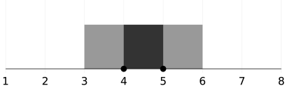
Figure 1: Hypothetical observed univariate data with $y_{1}=4$, $y_{2}=5$, and $n=2$. With nonconformity measure $\Psi(y^{n+1}_{-i},y_{i}):=|\text{mean}(y_{-i}^{n+1})-y_{i}|$, the inner black region represents the values of $y_{n+1}$ that would have rank 1 (i.e., $A_{n}(1)=\big{\{}y\,:\,\text{rank}(t_{n+1}(y))=1\big{\}}$), the outer grey region represents the values of $y_{n+1}\in A_{n}(2)=\big{\{}y\,:\,\text{rank}(t_{n+1}(y))=2\big{\}}$, and the outermost white region represents the values of $y_{n+1}\in A_{n}(n+1)=\big{\{}y\,:\,\text{rank}(t_{n+1}(y))=n+1\big{\}}$.

The imprecision in the GF distribution is that the probability mass $\mu$ is only defined for sets of values $A_{n}(v)\subseteq\mathbb{Y}$, for $v\in\{1,\dots,n+1\}$, rather than a mass or density function defined for all points in $\mathbb{Y}$, as in the precise probability scenario; and the imprecision comes from the fact that nothing is being assumed about the underlying distribution of the data. The novelty of the approach is that the GF framework is, nonetheless, versatile enough to provide inferences and construct CP sets, based on the model-free association (2) with the sole assumption of exchangeable, continuous data. Inferences are facilitated by the construction of belief and plausibility functions, denoted $\underline{\mu}$ and $\overline{\mu}$, respectively, so that for any event $B\subseteq\mathbb{Y}$ pertaining to the prediction of $y_{n+1}$, i.e., $\{y_{n+1}\,:\,B\ni y_{n+1}\}$,

$$\underline{\mu}(B) :=\sum_{j=1}^{n+1}\mu\{A_{n}(j)\}\cdot 1\big{\{}A_{n}(j)\subseteq B\big{\}},\text{ and}$$

$$\overline{\mu}(B) :=\sum_{j=1}^{n+1}\mu\{A_{n}(j)\}\cdot 1\big{\{}A_{n}(j)\cap B\neq\emptyset\big{\}}.$$

Demonstrating the construction of CP sets is a bit more involved, but amounts to a careful arrangement of the focal sets $A_{n}(1),\dots,A_{n}(n+1)$.

The important insight from Figure 1 is that the imprecise GF distribution of $y_{n+1}$ assigns, in particular, $1/(n+1)$ probability to the outermost region (beyond where any data were observed), and as such, it assigns $n/(n+1)$ probability to the complementary set (within which all of the data were observed). That being so, an $n/(n+1)$ probability GF prediction set is given by,

$$\Omega_{n}(k):=\bigcup_{1\leq v\leq k}A_{n}(v)=\big{\{}y\,:\,\text{rank}(t_{n+1}(y))\leq k\big{\}},$$

with $k=n$. Moreover, if $t_{1}(y_{1}),\dots,t_{n}(y_{n})$ are all unique values (i.e., under Assumption 1), then a $k/(n+1)$ GF prediction set is given by $\Omega_{n}(k)$, for any $k\in\{1,\dots,n+1\}$. Theorem 6, below, relates this model-free GF prediction set to a CP set via the GF transducer function:

$$f_{n}(y):=\mu\big{\{}\Omega_{n}(V^{\star})\ni y\big{\}}.$$ (5)

As a simple example, for the hypothetical data displayed in Figure 1, the GF transducer is

$$f_{n}(y)=\begin{cases}1&\text{ if }\ y\in(4,5)\\ \frac{2}{3}&\text{ if }\ y\in(3,4]\cup[5,6)\\ \frac{1}{3}&\text{ else }\end{cases}.$$

More interesting examples of GF transducers for synthetic Gaussian and Cauchy data are plotted in Figure 2. These plots are representative of the shape and interpretation of conformal transducers, more generally. The important implication of Theorem 6 is that $\Upsilon_{n}^{\alpha}:=\{y:f_{n}(y)>\alpha\}$ is a [type 1] valid, model-free GF prediction set, as stated in Corollary 7.

At any level $\alpha\in(0,1)$, the region $\Upsilon_{n}^{\alpha}$ is easily determined in the plots in Figure 2 by drawing a horizontal line at the value of $\alpha$ and including all values of $y$ that satisfy $f_{n}(y)>\alpha$ (i.e., $\Upsilon_{n}^{\alpha}$ is a pre-image set of $f_{n}$). Although a transducer is not understood as a density function, construction of $\Upsilon_{n}^{\alpha}$ is akin to the construction of high posterior density credible sets in Bayesian inference.

Theorem 6

Under Assumption 1 the GF transducer $f_{n}(Y_{n+1})$ is a conformal transducer.

Proof. This result is simply a statement of the fact that using $f_{n}(y_{n+1})$ in place of $p_{n+1}$ in Algorithm 1 defines a conformal algorithm. This follows because

$$\begin{split}f_{n}(y_{n+1})&=\mu\big{\{}\Omega_{n}(V^{\star})\ni y_{n+1}\big{\}}\\ &=\mu\big{\{}\text{rank}\{t_{n+1}(y_{n+1})\}\leq V^{\star}\big{\}}\\ &=\frac{n+1-\text{rank}\{t_{n+1}(y_{n+1})\}+1}{n+1}\\ &=\frac{n+1-1-\sum_{i=1}^{n+1}1\{t_{n+1}(y_{n+1})>t_{i}(y_{i})\}+1}{n+1}\\ &=\frac{n+1-\sum_{i=1}^{n+1}1\{t_{n+1}(y_{n+1})>t_{i}(y_{i})\}}{n+1}\\ &=\frac{\sum_{i=1}^{n+1}1\{t_{n+1}(y_{n+1})\leq t_{i}(y_{i})\}}{n+1}.\\ \end{split}$$ (6)

$\blacksquare$

Corollary 7

Under Assumption 1 the GF prediction set $\Upsilon_{n}^{\alpha}$ is [type 1] valid, as in Definition 1.

Proof. As shown in Theorem 6, $f_{n}(y_{n+1})$ is equivalent to $p_{n+1}$ in Algorithm 1, and so

$$P(\Upsilon_{n}^{\alpha}\not\ni Y_{n+1})=P\big{(}f_{n}(Y_{n+1})\leq\alpha\big{)}\leq\alpha,$$

as a direct consequence of Theorem 3. $\blacksquare$

It is clear from Theorem 6 that CP sets can be constructed from the GF inference paradigm, namely $\Upsilon_{n}^{\alpha}$ is a CP set. Furthermore, it follows from expression (6) that any CP set as constructed from Algorithm 1 can be understood as a union of sets from the imprecise GF probability distribution of $Y_{n+1}$ defined by (3). This fact establishes the strong connection between GF inference and CP. Beyond this connection, in a scenario where a point prediction is required, it is less clear how to use a CP set.

Certainly the finite sample validity property will be lost by mapping a CP set to a point, but within this new framework of model-free GF inference it is possible to construct a probability distribution over prediction points with desirable properties. This is not as simple as taking the center of each set $A_{n}(v)$ for $v\in\{1,\dots,n+1\}$ because $A_{n}(v)$ need not be convex. Further, the center of the nested sets $\Omega_{n}(k)=\bigcup_{1\leq v\leq k}A_{n}(v)$ includes the same point for every $k$, and so mapping $\Omega_{n}(k)$, i.e., a CP set, to a point prediction in this way would lead to a single point for all $k\in\{1,\dots,n+1\}$ (i.e., regardless of the desired significance level). The construction of a precise probabilistic approximation to the imprecise model-free GF predictive distribution is the topic of the next section.

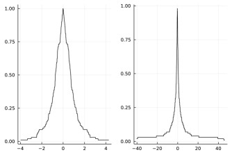
Figure 2: Both panels display plots of the GF transducer, $f_{n}(y)=\mu\big{\{}\Omega_{n}(V^{\star})\ni y\big{\}}$; the left and right plots are based on samples of $n=100$ realizations from the standard Gaussian and standard Cauchy distributions, respectively.

3 Mapping GF imprecise distributions to precise distributions

Although heuristic methods have been discussed and evaluated empirically (Hannig, 2009), mapping GF imprecise distributions to precise distributions has remained largely an open question for research in the GF literature. Recall the example of the imprecise GF distribution constructed for the parameter of a binomial distribution, in Section 2.2. The existing GF inference literature suggests mapping the imprecise GF distribution to a precise distribution by taking some point in the interval $(U_{(y)}^{\star},U_{(y+1)}^{\star}]$, which can be expressed as suggested in Hannig (2009) as

$$\mathcal{R}_{\theta}(y)=U_{(y)}^{\star}+D(U_{(y+1)}^{\star}-U_{(y)}^{\star}),$$

for some random variable $D$ supported on or in $[0,1]$. There are five options for the choice of $D$ discussed in Hannig (2009). The first is the maximum entropy $D\sim\text{uniform}(0,1)$, and the second is the maximum variance $D\sim\text{uniform}\{0,1\}$ which amounts to arithmetic averaging of the densities of the endpoints. The third choice is $D\sim\text{beta}(.5,.5)$ which leads to the Bayesian posterior of $\mathcal{R}_{\theta}(y)$ using the Jeffreys prior. This also corresponds to the geometric mean of the densities of the endpoints, and is advocated for by Schweder and Hjort (2016). The fourth choice is

$$D\mid U_{1}^{\star},\dots,U_{n}^{\star}=\begin{cases}0&\text{ with probability }U_{(y)}^{\star}\\ 1&\text{ with probability }1-U_{(y+1)}^{\star}\\ \text{uniform}(0,1)&\text{ with probability }U_{(y+1)}^{\star}-U_{(y)}^{\star}\end{cases},$$

resulting in $\mathcal{R}_{\theta}(y)\sim\text{beta}(y+1,n-y+1)$. The fifth choice is simply to take the midpoint of the interval (i.e., $D=.5$). It is observed in simulation studies presented in Hannig (2009) that the second choice is optimal in some sense, though, there is a lack of intuition for why it seems to work better than simply taking the midpoint of the interval between the auxiliary endpoints.

In this section, I map the model-free imprecise GF distribution defined by (3) to a [precise] probability distribution that is optimal in the sense that it is a maximum entropy distribution (MED), and I derive non-asymptotic, sub-exponential concentration inequalities that establish the root-$n$ consistency for estimation of the true distribution of the data.

A probability measure $\Delta$ is naturally considered compatible with $\mu$ if for every measurable set $B$, $\underline{\mu}(B)\leq\Delta(B)\leq\overline{\mu}(B).$ The set of all such probability measures is called the credal set of $\mu$, and can be expressed as

$$\mathscr{C}(\mu):=\big{\{}\Delta\,:\,\Delta(B)\leq\overline{\mu}(B),\text{ for any measurable set }B\big{\}}.$$

Further, this construction implies that any probability measure $\Delta\in\mathscr{C}(\mu)$ must assign the same probability mass as $\mu$ to any focal set of $\mu$. This fact is established as a direct consequence of Lemma 8.

Lemma 8

A probability measure $\Delta\in\mathscr{C}(\mu)$ if and only if $\Delta\{A_{n}(v)\}=\frac{1}{n+1}=\mu\{A_{n}(v)\}$, for every $v\in\{1,\dots,n+1\}$.

Proof. First, suppose that $\Delta\in\mathscr{C}(\mu)$. Then for any $v\in\{1,\dots,n+1\}$, using the fact that $A_{n}(1),\dots,A_{n}(n+1)$ are mutually disjoint,

$$\mu\{A_{n}(v)\} =\sum_{j=1}^{n+1}\mu\{A_{n}(j)\}1\big{\{}A_{n}(j)\subseteq A_{n}(v)\big{\}}$$

$$=\underline{\mu}\{A_{n}(v)\}$$

$$\leq\Delta\{A_{n}(v)\}$$

$$\leq\overline{\mu}\{A_{n}(v)\}$$

$$=\sum_{j=1}^{n+1}\mu\{A_{n}(j)\}1\big{\{}A_{n}(j)\cap A_{n}(v)\neq\emptyset\big{\}}$$

$$=\mu\{A_{n}(v)\}$$

The desired result follows by equation (4).

For the converse direction, assume that $\Delta\{A_{n}(v)\}=\frac{1}{n+1}$, for every $v\in\{1,\dots,n+1\}$. Then, for any measurable set $B$, using the fact that $A_{n}(1),\dots,A_{n}(n+1)$ are mutually disjoint and collectively exhaustive over $\mathbb{Y}$,

$$\Delta(B) =\sum_{v=1}^{n+1}\Delta\big{\{}B\cap A_{n}(v)\big{\}}$$

$$\leq\sum_{v=1}^{n+1}\Delta\{A_{n}(v)\}1\big{\{}A_{n}(v)\cap B\neq\emptyset\big{\}}$$

$$=\sum_{v=1}^{n+1}\frac{1}{n+1}1\big{\{}A_{n}(v)\cap B\neq\emptyset\big{\}}$$

$$=\sum_{v=1}^{n+1}\mu\{A_{n}(v)\}1\big{\{}A_{n}(v)\cap B\neq\emptyset\big{\}}$$

$$=\overline{\mu}(B).$$

$\blacksquare$

The implication of interest of Lemma 8 is that any probability measure compatible with the imprecise GF mass function $\mu$ must assign uniform (i.e., $\frac{1}{n+1}$) probability to each of the mutually disjoint and collectively exhaustive regions $A_{n}(1),\dots,A_{n}(n+1)$. Assuming a density function exists, the probability density associated with any $\Delta\in\mathscr{C}(\mu)$, however, can have arbitrary shape over each region $A_{n}(v)$, subject to the constraint that it integrates to $\frac{1}{n+1}$. As such, in the absence of a model or any a-priori information, an optimal choice of probability measure in the credal set would be one that is least informative, e.g., in the sense of maximizing entropy. It is well-known that the MED over a bounded interval is uniform, and so the MED over the credal set $\mathscr{C}(\mu)$ should have a density $\pi^{n}_{y}$ that is flat over each focal set $A_{n}(v)$. Such a construction might require the modification of $A_{n}(1)$ and/or $A_{n}(n+1)$ so that the support of $\pi^{n}_{y}$ is restricted to $[\kappa_{n}^{\min},\kappa_{n}^{\max}]$ for arbitrarily small/large data-dependent choices of $\kappa_{n}^{\min}$ and $\kappa_{n}^{\max}$, so that uniform densities will integrate over these focal regions. The density function is derived by integrating the conditional uniform density on every focal set with respect to the GF mass function associated with the auxiliary variable: for $y\in[\kappa_{n}^{\min},\kappa_{n}^{\max}]$,

$$\pi^{n}_{y}(y) =\sum_{v=1}^{n+1}\pi^{n}_{y\mid v}(y\mid v)\cdot\pi^{n}_{v}(v)=\sum_{v=1}^{n+1}\begin{cases}\frac{1}{\lambda\{A_{n}(v)\}}\cdot\frac{1}{n+1}1\big{\{}y\in A_{n}(v)\big{\}}&\text{ if }|A_{n}(v)|>1\\ \delta_{A_{n}(v)}(y)\cdot\frac{1}{n+1}&\text{ if }|A_{n}(v)|=1\\ \end{cases},$$ (7)

where $\lambda$ is the Lebesgue measure on $\mathbb{Y}$, $|\cdot|$ denotes the cardinality of a set-valued argument, and $\delta_{A_{n}(v)}(\cdot)$ is the Dirac delta function for a singleton set $A_{n}(v)$, centered at the single point in $A_{n}(v)$. As established shortly, in Theorem 10, $\pi^{n}_{y}$ is in fact the density associated with the MED over $\mathscr{C}(\mu)$. Moreover, sampling from this distribution is intuitive, and is described by Algorithm 2.

An analogous sampling procedure to Algorithm 2 can be constructed to define a precise predictive distribution corresponding directly to the CP sets, i.e., sampling from $\Omega_{n}(v^{\star})$ rather than $A_{n}(v^{\star})$ in Algorithm 2. A comparison of such a CP predictive distribution versus the $\pi^{n}_{y}$ distribution is illustrated in Figures 3, 4, and 5 for Gaussian, Cauchy, and mixture of Gaussian data, respectively. The transducer function $f_{n}$, as in equation (5), for each of the three data sets, is plotted as a black line overlaying the histogram of samples drawn from $\pi^{n}_{y}$ and the CP-based analogue. The comparison of these two distributions is insightful for how the model-free GF precise approximation $\pi^{n}_{y}$ ameliorates a shortcoming of the elliptical symmetry of CP sets, more generally, as is best illustrated by Figure 5. A CP set constructed from sufficiently many data examples from a bi-modal distribution will include the region between the modes, even if no data is observed in this region. This is because $\Omega_{n}(1)\subseteq\Omega_{n}(2)\subseteq\cdots\subseteq\Omega_{n}(n+1)$, whereas $\pi^{n}_{y}$ is uniform over each of the disjoint regions $A_{n}(1),\dots,A_{n}(n+1)$ and is thus able to recover both modes observed from the data.

Input: Prediction regions $A_{n}(1),\dots,A_{n}(n+1)$.

Output: A realized instance of the random variable $Y_{n+1}$ with density function $\pi^{n}_{y}$.

1 Sample $v^{\star}\sim\text{uniform}\{1,\dots,n+1\}$;

2 Sample $y^{\star}\sim\text{uniform}\{A_{n}(v^{\star})\}$;

3 return $y^{\star}$;

Algorithm 2 Sampling according to the MED density $\pi^{n}_{y}$ from equation (7).

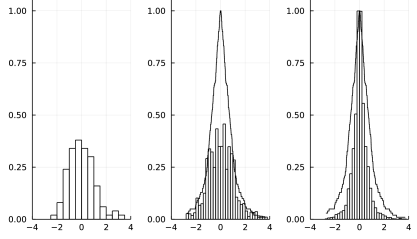
Figure 3: Based on the $n=100$ data points drawn from the standard Gaussian distribution, as summarized by the histogram in the left panel, the middle and right panels display histograms of samples of size 10,000 drawn, respectively, from Algorithm 2 and the CP-based analogue, i.e., replacing $A_{n}(v^{\star})$ with $\Omega_{n}(v^{\star})$. The nonconformity measure is $t_{i}(y_{i}):=|\text{mean}(y_{-i}^{n+1})-y_{i}|$. For reference, the transducer function is provided as the black line in the middle and right panels.

The intuition for why uniform sampling from the disjoint focal sets $A_{n}(1),\dots,A_{n}(n+1)$ is correct in some sense is that they will be narrower and clustered in regions of high probability density, wider and fewer in regions of low probability density, and the Lebesgue measure of $A_{n}(v)$ will converge to its probability measure associated with the true distribution of the data. This fact is formalized in Theorem 12 for nonconformity measure $t_{i}(Y_{i}):=Y_{i}$, but first I will establish the result that $\pi^{n}_{y}$ is the density associated with the MED. Denoting $\Pi^{n}_{y}(B):=\int_{B}\pi^{n}_{y}(y)\,dy$ for any Lebesgue measurable set $B$, to show that $\Pi^{n}_{y}$ is the MED over $\mathscr{C}(\mu)$, it must first be demonstrated, as in Lemma 9, that $\Pi^{n}_{y}\in\mathscr{C}(\mu)$.

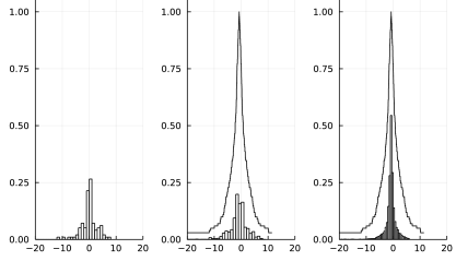
Figure 4: Based on the $n=100$ data points drawn from the standard Cauchy distribution, as summarized by the histogram in the left panel, the middle and right panels display histograms of samples of size 10,000 drawn, respectively, from Algorithm 2 and the CP-based analogue, i.e., replacing $A_{n}(v^{\star})$ with $\Omega_{n}(v^{\star})$. The nonconformity measure is $t_{i}(y_{i}):=|\text{mean}(y_{-i}^{n+1})-y_{i}|$. For reference, the transducer function is provided as the black line in the middle and right panels.

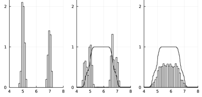
Figure 5: Based on the $n=100$ data points drawn from a mixture of two Gaussian distributions, as summarized by the histogram in the left panel, the middle and right panels display histograms of samples of size 10,000 drawn, respectively, from Algorithm 2 and the CP-based analogue, i.e., replacing $A_{n}(v^{\star})$ with $\Omega_{n}(v^{\star})$. The nonconformity measure is $t_{i}(y_{i}):=|\text{mean}(y_{-i}^{n+1})-y_{i}|$. For reference, the transducer function is provided as the black line in the middle and right panels.

Lemma 9

The probability measure $\Pi^{n}_{y}\in\mathscr{C}(\mu)$.

Proof. For any $j\in\{1,\dots,n+1\}$,

$$\Pi^{n}_{y}\{A_{n}(j)\}=\int_{A_{n}(j)}\pi^{n}_{y}(y)\,dy=\begin{cases}\int_{A_{n}(j)}\frac{1}{\lambda\{A_{n}(j)\}}\cdot\frac{1}{n+1}\,dy=\frac{1}{n+1}&\text{ if }|A_{n}(j)|>1\\ \int_{A_{n}(j)}\delta_{A_{n}(j)}(y)\cdot\frac{1}{n+1}\,dy=\frac{1}{n+1}&\text{ if }|A_{n}(j)|=1\end{cases}.$$

Thus, $\Pi^{n}_{y}\in\mathscr{C}(\mu)$ as a consequence of Lemma 8. $\blacksquare$

Theorem 10

The probability distribution associated with density function $\pi^{n}_{y}$ is the MED over all probability measures in $\mathscr{C}(\mu)$, supported on $[\kappa_{n}^{\min},\kappa_{n}^{\max}]$.

Proof. As illustrated by Lemma 8, the MED has a density residing in the set of density functions $\mathscr{Q}$ such that for every $q\in\mathscr{Q}$ and for every $v\in\{1,\dots,n+1\}$,

$$\int_{A_{n}(v)}q(y)\,dy=\frac{1}{n+1}.$$

If $|A_{n}(v)|=1$, then it must be the case that $q(y)=\delta_{A_{n}(v)}(y)\cdot\frac{1}{n+1}$ for $y\in A_{n}(v)$. Alternatively, over the non-singleton focal set regions, the MED over $\mathscr{C}(\mu)$ can be found via the method of Lagrange multipliers constrained to the set $\mathscr{Q}$. The constrained entropy functional has the form

$$J[q]=-\int_{\kappa_{n}^{\min}}^{\kappa_{n}^{\max}}q(y)\log\{q(y)\}\,dy+\sum_{j\,:\,|A_{n}(j)|>1}\beta_{j}\Bigg{[}\int_{A_{n}(j)}q(y)\,dy-\frac{1}{n+1}\Bigg{]},$$

and can be minimized using standard techniques from calculus of variations (a standard text on this subject is Gelfand and Fomin, 2000). The first-order condition for an optimum, based on the functional derivative is

$$\frac{\delta J}{\delta q}=-\log\{q(y)\}-1+\sum_{j\,:\,|A_{n}(j)|>1}\beta_{j}1\{y\in A_{n}(j)\}=0.$$

Thus, the MED density has the form $q(y)=e^{-1+\sum_{j\,:\,|A_{n}(j)|>1}\beta_{j}1\{y\in A_{n}(j)\}},$ subject to the constraint

$$\frac{1}{n+1} =\int_{A_{n}(v)}e^{-1+\sum_{j\,:\,|A_{n}(j)|>1}\beta_{j}1\{y\in A_{n}(j)\}}\,dy=\int_{A_{n}(v)}e^{-1+\beta_{v}}\,dy=e^{-1+\beta_{v}}\lambda\{A_{n}(v)\},$$

and so $q(y)=\frac{1}{\lambda\{A_{n}(v)\}}\cdot\frac{1}{n+1}$ for $y\in A_{n}(v)$ for every $v\in\{1,\dots,n+1\}$. Therefore,

$$q(y) =\sum_{v=1}^{n+1}\begin{cases}\frac{1}{\lambda\{A_{n}(v)\}}\cdot\frac{1}{n+1}1\big{\{}y\in A_{n}(v)\big{\}}&\text{ if }|A_{n}(v)|>1\\ \delta_{A_{n}(v)}(y)\cdot\frac{1}{n+1}&\text{ if }|A_{n}(v)|=1\\ \end{cases}$$

$$=\pi^{n}_{y}(y).$$

$\blacksquare$

The next two results demonstrate the non-asymptotic, sub-exponential concentration that establishes the root-$n$ consistency of the model-free GF precise approximation for estimation of the true distribution of the data, in the case that the nonconformity score is taken to be each datum itself, i.e., $t(Y_{i}):=Y_{i}$. In particular, Theorem 11 demonstrates that point-wise, $\Pi^{n}_{y}\{(-\infty,y]\}-F(y)=o_{p}(n^{-\gamma})$, for any $\gamma\in[0,0.5)$, where $F$ is the distribution function associated with the true distribution of $Y_{n+1}\sim P$. Theorem 12 establishes an even faster rate of convergence on the focal sets; $\Pi^{n}_{y}\{A_{n}(v)\}-P\{A_{n}(v)\}=o_{p}(n^{-\tau})$, for any $\tau\in[0,1)$. See Figure 6 for an empirical illustration of the consistency in a few synthetic data examples.

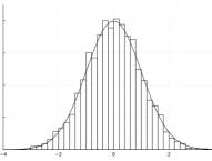
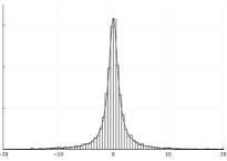
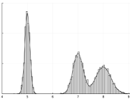
Figure 6: Histograms of samples from $\pi_{y}^{n}$ computed by Algorithm 2, and based on data sets of size $n=10,000$ from the standard Gaussian distribution (left panel), standard Cauchy distribution (middle panel), and a mixture distribution (right panel). The nonconformity measure is $t(y_{i}):=y_{i}$. The black lines are plots of the respective density functions associated with the data.

Theorem 11

Let $Y_{1},\dots,Y_{n}\overset{\text{iid}}{\sim}P$ be a collection of continuous random variables, $t_{i}(Y_{i}):=Y_{i}$ for $i\in\{1,\dots,n\}$, $\kappa_{n}^{\min}:=Y_{(1)}$, and $\kappa_{n}^{\max}:=Y_{(n)}$. For any $y\in\mathbb{R}$, $\gamma\in[0,0.5)$, $\epsilon>0$, and for all $n>4n^{\gamma}/\epsilon-1$,

$$P\Big{(}n^{\gamma}\big{|}\Pi^{n}_{y}\{(-\infty,y]\}-F(y)\big{|}>\epsilon\Big{)}\leq\Big{[}2e^{-\frac{\epsilon^{2}}{8}n^{1-2\gamma}}+e^{-nF(y)}\Big{]}\cdot 1\{F(y)>0\}.$$

Proof. Denote $B:=(-\infty,y]$ and first observe that

$$B\cap\bigcup_{j=1}^{n+1}A_{n}(j)=\begin{cases}\emptyset&\text{ if }y<\kappa_{n}^{\min}=Y_{(1)}\\ A_{n}(1)&\text{ if }Y_{(1)}=y\\ \Big{[}\bigcup_{j=1}^{M_{n}-1}A_{n}(j)\Big{]}\cup\big{\{}B\cap A_{n}(M_{n})\big{\}}&\text{ if }Y_{(1)}<y\end{cases},$$

where $M_{n}$ is the number of focal sets having a nonempty intersection with $B$:

$$M_{n}:=\big{|}\big{\{}v\,:\,(-\infty,y]\cap A_{n}(v)\neq\emptyset\big{\}}\big{|},$$

satisfies $Z_{n}:=M_{n}-1\{M_{n}>0\}\sim\text{binomial}(n,p_{B})$, where $p_{B}:=P(B)$. Next, by definition,

$$\Pi^{n}_{y}(B)=\begin{cases}0&\text{ if }y<\kappa_{n}^{\min}=Y_{(1)}\\ (M_{n}-1)\cdot\frac{1}{n+1}+\Pi^{n}_{y}\big{\{}B\cap A_{n}(M_{n})\big{\}}&\text{ if }Y_{(1)}\leq y\end{cases},$$

noting that $B\cap A_{n}(1)=A_{n}(1)=\{Y_{(1)}\}$. Accordingly,

$$P\Big{(}n^{\gamma}\big{|}\Pi^{n}_{y}(B)-P(B)\big{|}>\epsilon\Big{)} =P\Bigg{(}\bigg{|}\Pi^{n}_{y}(B)-\frac{M_{n}-1}{n+1}+\frac{M_{n}-1}{n+1}-p_{B}\bigg{|}>\epsilon/n^{\gamma}\Bigg{)}$$

$$\leq P\Bigg{(}M_{n}>0,\bigg{|}\Pi^{n}_{y}\big{\{}B\cap A_{n}(M_{n})\big{\}}+\frac{M_{n}-1}{n+1}-p_{B}\bigg{|}>\epsilon/n^{\gamma}\Bigg{)}$$

$$\hskip 36.135pt+P(M_{n}=0)$$

$$\leq P\bigg{(}M_{n}>0,\Pi^{n}_{y}\big{\{}B\cap A_{n}(M_{n})\big{\}}>\frac{\epsilon}{2n^{\gamma}}\bigg{)}$$

$$\hskip 36.135pt+P\Bigg{(}M_{n}>0,\bigg{|}\frac{M_{n}-1}{n+1}-p_{B}\bigg{|}>\frac{\epsilon}{2n^{\gamma}}\Bigg{)}+(1-p_{B})^{n}$$

$$\leq 1\bigg{\{}\frac{1}{n+1}>\frac{\epsilon}{2n^{\gamma}}\bigg{\}}+P\Bigg{(}\bigg{|}\frac{Z_{n}}{n+1}-p_{B}\bigg{|}>\frac{\epsilon}{2n^{\gamma}}\Bigg{)}+(1-p_{B})^{n}$$

$$\leq P\bigg{(}|Z_{n}-n\cdot p_{B}|+p_{B}>\frac{(n+1)\epsilon}{2n^{\gamma}}\bigg{)}+(1-p_{B})^{n}$$

$$\leq P\bigg{(}|Z_{n}-E(Z_{n})|>\frac{(n+1)\epsilon}{4n^{\gamma}}\bigg{)}+(1-n\cdot p_{B}/n)^{n}$$

$$\leq 2e^{-\frac{\epsilon^{2}}{8}n^{1-2\gamma}}+e^{-n\cdot p_{B}},$$

where the last approximation is an application of the Hoeffding inequality. $\blacksquare$

Theorem 12

Let $Y_{1},\dots,Y_{n}\overset{\text{iid}}{\sim}P$ be a collection of continuous random variables, $t_{i}(Y_{i}):=Y_{i}$ for $i\in\{1,\dots,n\}$, $\kappa_{n}^{\min}:=Y_{(1)}$, and $\kappa_{n}^{\max}:=Y_{(n)}$. Then for any $\tau\in[0,1)$, for any $\epsilon>0$,

$$P\Big{(}n^{\tau}\big{|}\Pi^{n}_{y}\{A_{n}(v)\}-P\{A_{n}(v)\}\big{|}>\epsilon\Big{)}=\begin{cases}1-(1-b_{n})^{n}+(1-c_{n})^{n}&\text{ for }v\in\{2,\dots,n\}\\ 1\big{\{}\frac{n^{\tau}}{n+1}>\epsilon\big{\}}&\text{ for }v\in\{1,n+1\}\end{cases},$$

where $b_{n}:=\max\big{\{}\frac{1}{n+1}-\frac{\epsilon}{n^{\tau}},0\big{\}}$, $c_{n}:=\min\big{\{}\frac{1}{n+1}+\frac{\epsilon}{n^{\tau}},1\big{\}}$. In particular, for all $n>\max\big{\{}\frac{n^{\tau}-\epsilon}{\epsilon},\frac{\epsilon}{n^{\tau}-\epsilon}\big{\}}$,

$$P\Big{(}n^{\tau}\big{|}\Pi^{n}_{y}\{A_{n}(v)\}-P\{A_{n}(v)\}\big{|}>\epsilon\Big{)} \leq e^{-n^{1-\tau}\epsilon}.$$

Proof. Let $F$ denote the cumulative distribution function associated with $P$. Due to the continuity of $F$ and the independence of the data, for any $v\in\{2,\dots,n\}$, $W_{n}:=F(Y_{(v)})-F(Y_{(v-1)})\sim\text{beta}(1,n).$ Then,

$$P\Big{(}n^{\tau}\big{|}\Pi^{n}_{y}\{A_{n}(v)\}-P\{A_{n}(v)\}\big{|}>\epsilon\Big{)} =P\Bigg{(}n^{\tau}\bigg{|}\frac{1}{n+1}-\big{[}F(Y_{(v)})-F(Y_{(v-1)})\big{]}\bigg{|}>\epsilon\Bigg{)}$$ (8)

$$=1-P\Bigg{(}\bigg{|}W_{n}-\frac{1}{n+1}\bigg{|}\leq\frac{\epsilon}{n^{\tau}}\Bigg{)}$$

$$=1-P\big{(}b_{n}\leq W_{n}\leq c_{n}\big{)}.$$

Next,

$$P\big{(}b_{n}\leq W_{n}\leq c_{n}\big{)} =\int_{b_{n}}^{c_{n}}n(1-x)^{n-1}\,dx=-(1-x)^{n}\,\bigg{|}_{b_{n}}^{c_{n}}=(1-b_{n})^{n}-(1-c_{n})^{n},$$

so that

$$P\Big{(}n^{\tau}\big{|}\Pi^{n}_{y}\{A_{n}(v)\}-P\{A_{n}(v)\}\big{|}>\epsilon\Big{)} =1-(1-b_{n})^{n}+(1-c_{n})^{n}$$

$$\leq 1-(1-b_{n})^{n}+e^{-nc_{n}}.$$

For $v\in\{1,n+1\}$, denote $Y_{(0)}:=\kappa_{n}^{\min}=Y_{(1)}$, and $Y_{(n+1)}:=\kappa_{n}^{\max}=Y_{(n)}$, and simplify equation (8). $\blacksquare$

4 Numerical examples

In this section, I present two synthetic simulation experiments to motivate the relevance of the model-free imprecise GF inference approach that I have constructed and proposed in the developments throughout this manuscript, along with that of the model-free GF precise probabilistic approximation. These numerical examples are manifestations of practical applications where making [finite sample] valid predictions is critical, and (i) where a standard Bayesian solution would result in unsuspecting mis-quantification of uncertainty; (ii) where CP solution is limited by its lack of versatility; and (iii) where the model-free GF approaches are reliable, nonetheless.

The premise of the numerical examples that follow are the unexceptional but under-appreciated consequences of model mis-specification. Specifically, suppose that a practitioner is given a data set of $n$ realizations from some waiting-time distribution, and tasked with making a prediction inference in quantifying the uncertainty of a high-stakes decision. More precise scenarios will follow, but for each scenario, assume that the data $Y_{1},\dots,Y_{n}\overset{\text{iid}}{\sim}\text{log-normal}(1,2)$ and that the true log-normal(1,2) distribution is unknown. The canonical parametric model for waiting-time data is an exponential$(\theta)$ distribution, analogous to how a Gaussian distribution is the canonical parametric model for real-valued data. That being so, it is foreseeable that a practitioner might unsuspectingly fit an exponential$(\theta)$ distribution to data that are actually log-normally distributed; for a perspective, Figure 7 displays histograms of four realizations of $n=10,000$ independently sampled data sets from the log-normal(1,2) distribution, overlayed with the density curve of the exponential distribution fitted at the maximum likelihood estimate. Certain consequences of such model mis-specification are illustrated in scenarios to follow, and it is exhibited that the model-free GF approaches remain reliable. In fact, neither the model-free GF imprecise nor precise formulation assume any model specification.

4.1 Example: Prediction inference in longitudinal studies

The conjugate prior for an iid sample from an exponential$(\theta)$ model is a gamma distribution, and the posterior predictive distribution works out analytically as a Lomax distribution. The cumulative distribution function for the Lomax$(\alpha,\gamma)$ distribution has the form $\widetilde{F}(y)=1-(1+y/\lambda)^{-\alpha}$, supported on $y\geq 0$. For humans afflicted with a certain disease, assume that log-normal(1,2) is the population model for the time in days until treatment for the disease becomes necessary to avoid permanent or life threatening health consequences. Further, suppose that there is an excessive cost to the medical infrastructure if wide-spread availability of treatment resources is necessary within two-days from exposure to the disease. To assess whether the cost is warranted, public health officials might need to make a prediction about the incubation period of the disease and quantify the uncertainty of the event that it is less than two-days, i.e., the event $B:=[0,2]$. Figure 8 provides a comparison of the posterior predictive probability of $B$ versus the model-free GF belief, plausibility, and precise approximation probability of $B$, for a grid of samples sizes, and averaged over 1,000 synthetic data sets. Recall that Figure 7 provides a general characterization of the synthetic data sets. As evident in Figure 8, the model-free GF approaches accurately and efficiently estimate the true log-normal(1,2) probability of the event $B$, while the canonical Bayesian posterior predictive probability exhibits considerable bias. The apparent consequence of the mis-specification for the Bayesian approach is the quantification of 0.8 to 0.9 probability that the incubation time exceeds two-days, whereas the true probability of incubation within two days is nearly 0.45; and the mis-quantification of uncertainty only gets worse as the sample size increases.

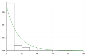
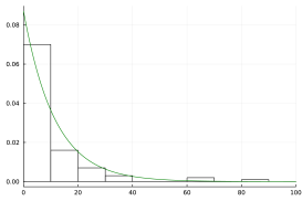
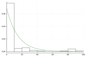
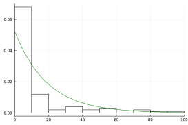
Figure 7: Each panel is one of four expository histograms of realizations of $n=10,000$ independently sampled data sets from the log-normal(1,2) distribution, overlayed with the density curve of the exponential distribution fitted at the maximum likelihood estimate.

It is easy to find real scenarios where this simulation study construction is plausibly relevant. For instance, the administration of immune globulin followed by a series of vaccination injections is imperative to survival following a rabies exposure, and the effectiveness of the treatment requires that it is administered during the incubation period for the virus. Reliable uncertainly quantification pertaining to the likely duration of the incubation period has serious public health consequences, and can be used by epidemiologists to provide guidelines to clinicians and the public about how soon an individual should seeks treatment. Of course, an obvious guideline is to seek treatment immediately, but that many be excessively costly; e.g., the rabies immune globulin is a very expensive medication for medical institutions to keep in stock, making the uncertainty quantification of the incubation period critical to a resource allocation problem. Other examples could include the reliable uncertainly quantification pertaining to (i) the progression time of skin cancers, resulting in public health guidelines for how often people should schedule regular screenings with a dermatologist; or (ii) the dissolving time of nitrogen bubbles due to the effects of pressure at depth for scuba divers, leading to recommendations for “safety stop” durations to lower the risk of decompression sickness (i.e., “the bends”).

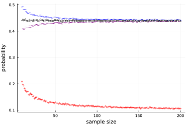
Figure 8: Uncertainty quantification of the event $B:=[0,2]$, averaged over 1,000 simulations of data sets $Y_{1},\dots,Y_{n}\overset{\text{iid}}{\sim}\text{log-normal}(1,2)$, for each sample size $n\in\{10,11,\dots,200\}$. The true log-normal(1,2) probability of $B$ is unrelated to any observed data set, but is plotted for reference as the horizontal black line; red crosses denote the Lomax-distributed posterior predictive probability of $B$; black circles denote $\Pi_{y}^{n}(B)$; purple dashes denote $\underline{\mu}(B)$; and blue dashes denote $\overline{\mu}(B)$.

4.2 Example: Prediction inference in survival analysis

The setup of this second simulation study is the same as that of the previous section, but the premise is instead that inference is desired on a survival time, i.e., inference on the event $[t,\infty)$ for $t>0$. A comparison of the approaches is displayed in Figure 9, and the consequences of model mis-specification for the canonical Bayesian solution persist, whilst model-free GF approaches remain reliable and efficient.

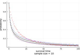
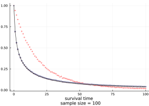
Figure 9: Uncertainty quantification of survival to time $t$ for $t\in\{0,1,\dots,100\}$, averaged over 1,000 simulations of data sets $T_{1},\dots,T_{n}\overset{\text{iid}}{\sim}\text{log-normal}(1,2)$, for each sample size $n=10$ (left panel) and $n=100$ (right panel). The true log-normal(1,2) survival probability, $1-F(t)$, is unrelated to any observed data set, but is plotted for reference as the horizontal black line; red crosses denote the Lomax-distributed posterior predictive probability $1-\widetilde{F}(t)$; black circles denote $\Pi_{y}^{n}\{[t,\infty)\}$; purple dashes denote $\underline{\mu}\{[t,\infty)\}$; and blue dashes denote $\overline{\mu}\{[t,\infty)\}$.

5 Concluding remarks

The problem of mapping imprecise probability measures to precise probability approximations has been considered, more broadly, in the approximate reasoning research community. For example, Dubois et al. (2004) provides conditions and theorems for transformation between possibility/necessity measures and probability measures, where a possibility measure of an event $B$ is defined by the supremum of a transducer or contour function over all points in $B$. Possibility/necessity measures are a special class of upper/lower probabilities, analogous to how plausibility/belief measures are upper/lower probabilities. There remain, however, many open research questions concerning precise probability approximations, from a statistical inference perspective. Perhaps exploring (beyond the developments in the preceding sections) optimization strategies in a new research area of calculus of variations on credal sets will be fruitful for new constructions of precise probabilistic approximations guided by reliability and accountability in uncertainty quantification.

Appendix A

Proof of Theorem 3. Any realization of nonconformity scores $t_{1}(y_{1}),\dots,t_{n+1}(y_{n+1})$ can be described as a collection containing unique values, $a_{1},\dots,a_{K}$, for some $K\leq n+1$ and occurring with frequencies $n_{1},\dots,n_{K}$, respectively (with $\sum_{k=1}^{K}n_{k}=n+1$). Using the fact that $t_{1}(Y_{1}),\dots,t_{n+1}(Y_{n+1})$ are exchangeable (because $Y_{1},\dots,Y_{n+1}$ are exchangeable) as in Definition 2, it follows by definition that any realization $t_{1}(y_{1}),\dots,t_{n+1}(y_{n+1})$ can be understood as some permutation of the values in the bag (i.e., a collection of elements with no ordering),

$$B:=\lbag\underbrace{a_{(1)},\dots,a_{(1)}}_{n_{1}},\underbrace{a_{(2)},\dots,a_{(2)}}_{n_{2}},\dots,\underbrace{a_{(K)},\dots,a_{(K)}}_{n_{K}}\rbag,$$

where $a_{(k)}$ is the $k$-th order statistic (in ascending order) of the values $a_{1},\dots,a_{K}$. As such, the observed nonconformity scores $t_{1}(y_{1}),\dots,t_{n+1}(y_{n+1})$ are just one of $(n+1)!$ equally possible permutations that the could have been recorded, assuming $y_{n+1}$ was generated from equation (1).

Next, with reference to the bag $B$ it can be determined that

$$\sum_{i=1}^{n+1}1\{t_{i}(y_{i})\geq t_{n+1}(y_{n+1})\}=\begin{cases}n+1&\text{ if }\ t_{n+1}(y_{n+1})=a_{(1)}\\ n+1-n_{1}&\text{ if }\ t_{n+1}(y_{n+1})=a_{(2)}\\ n+1-n_{1}-n_{2}&\text{ if }\ t_{n+1}(y_{n+1})=a_{(3)}\\ &\vdots\\ n_{K}&\text{if }\ t_{n+1}(y_{n+1})=a_{(K)}\end{cases}.$$

Furthermore, there are $n!\cdot n_{j}$ permutations of the values in $B$ in which the last reported value, $t_{n+1}(y_{n+1})=a_{(j)}$, so it must be the case that

$$P\bigg{(}\sum_{i=1}^{n+1}1\{t_{i}(Y_{i})\geq t_{n+1}(Y_{n+1})\}=v\ \Big{|}\ B\bigg{)}=\begin{cases}\frac{n!\cdot n_{1}}{(n+1)!}=\frac{n_{1}}{n+1}&\text{ if }\ v=n+1\\ \frac{n!\cdot n_{2}}{(n+1)!}=\frac{n_{2}}{n+1}&\text{ if }\ v=n+1-n_{1}\\ \frac{n!\cdot n_{3}}{(n+1)!}=\frac{n_{3}}{n+1}&\text{ if }\ v=n+1-n_{1}-n_{2}\\ &\vdots\\ \frac{n!\cdot n_{K}}{(n+1)!}=\frac{n_{K}}{n+1}&\text{ if }\ v=n_{K}\\ 0&\text{ else }\end{cases}.$$

Note that in the special case without repeated values (i.e., $n_{1}=\cdots=n_{K}=1$), the above expression reduces to a discrete uniform probability mass function. In any case,

$$P(\Gamma_{n}^{\alpha}\not\ni Y_{n+1}\mid B) =P(p_{n+1}\leq\alpha\mid B)$$

$$=P\bigg{(}\sum_{i=1}^{n+1}1\{t_{i}(Y_{i})\geq t_{n+1}(Y_{n+1})\}\leq\alpha(n+1)\ \Big{|}\ B\bigg{)}$$

$$=\begin{cases}\frac{n_{K}}{n+1}+\frac{n_{K-1}}{n+1}+\cdots+\frac{n_{k_{\alpha}+1}}{n+1}&\text{ if }k_{\alpha}<K\\ 0&\text{ if }k_{\alpha}=K\end{cases},$$

where $k_{\alpha}:=\min\big{\{}j\in\{0,\dots,K\}\,:\,n+1-\sum_{k=0}^{j}n_{k}\leq\alpha(n+1)\big{\}}$ and $n_{0}:=0$. Observe from the construction of $k_{\alpha}$ that,

$$n_{K}+n_{K-1}+\cdots+n_{k_{\alpha}+1}=n+1-\sum_{k=0}^{k_{\alpha}}n_{k}\leq\alpha(n+1),$$

and divide by $n+1$ on all sides. Thus, in any case,

$$P(\Gamma_{n}^{\alpha}\not\ni Y_{n+1})=\int P(\Gamma_{n}^{\alpha}\not\ni Y_{n+1}\mid B)d\nu(B)\leq\alpha\cdot\int d\nu(B)=\alpha,$$

where $\nu(\cdot)$ is any probability measure that described the uncertainty in observing the bag $B$. $\blacksquare$

References

- Balch et al. (2019) M. S. Balch, R. Martin, and S. Ferson. Satellite conjunction analysis and the false confidence theorem. Proceedings of the Royal Society A, 475(20180565), 2019.
- Basir and Yuan (2007) O. Basir and X. Yuan. Engine fault diagnosis based on multi-sensor information fusion using Dempster-Shafer evidence theory. Information fusion, 8(4):379–386, 2007.
- Begoli et al. (2019) E. Begoli, T. Bhattacharya, and D. Kusnezov. The need for uncertainty quantification in machine-assisted medical decision making. Nature Machine Intelligence, 1(1):20–23, 2019.
- Bloch (1996) I. Bloch. Some aspects of Dempster-Shafer evidence theory for classification of multi-modality medical images taking partial volume effect into account. Pattern Recognition Letters, 17(8):905–919, 1996.
- Carmichael and Williams (2018) I. Carmichael and J. P. Williams. An exposition of the false confidence theorem. Stat, 7(1):e201, 2018.
- Cella and Martin (2022a) L. Cella and R. Martin. Validity, consonant plausibility measures, and conformal prediction. International Journal of Approximate Reasoning, 141:110–130, 2022a.
- Cella and Martin (2022b) L. Cella and R. Martin. Direct and approximately valid probabilistic inference on a class of statistical functionals. International Journal of Approximate Reasoning, 151:205–224, 2022b.
- Dempster (1966) A. P. Dempster. New methods for reasoning towards posterior distributions based on sample data. The Annals of Mathematical Statistics, 37(2):355–374, 1966.
- Denoeux (2000) T. Denoeux. A neural network classifier based on Dempster-Shafer theory. IEEE Transactions on Systems, Man, and Cybernetics-Part A: Systems and Humans, 30(2):131–150, 2000.
- Denoeux (2008) T. Denoeux. A k-nearest neighbor classification rule based on Dempster-Shafer theory. In Classic works of the Dempster-Shafer theory of belief functions, pages 737–760. Springer, 2008.
- Díaz-Más et al. (2010) L. Díaz-Más, R. Muñoz-Salinas, F. J. Madrid-Cuevas, and R. Medina-Carnicer. Shape from silhouette using Dempster-Shafer theory. Pattern Recognition, 43(6):2119–2131, 2010.
- Dubois et al. (2004) D. Dubois, L. Foulloy, G. Mauris, and H. Prade. Probability-possibility transformations, triangular fuzzy sets, and probabilistic inequalities. Reliable computing, 10(4):273–297, 2004.
- Elemento et al. (2021) O. Elemento, C. Leslie, J. Lundin, and G. Tourassi. Artificial intelligence in cancer research, diagnosis and therapy. Nature Reviews Cancer, 21(12):747–752, 2021.
- Ford and Gregory (2006) E. B. Ford and P. C. Gregory. Bayesian model selection and extrasolar planet detection. arXiv preprint astro-ph/0608328, 2006.
- Gelfand and Fomin (2000) I. Gelfand and S. Fomin. Calculus of variations,(translated and edited by silverman, ra), 2000.
- Hannig (2009) J. Hannig. On generalized fiducial inference. Statistica Sinica, pages 491–544, 2009.
- Hannig et al. (2016) J. Hannig, H. Iyer, R. C. Lai, and T. C. Lee. Generalized fiducial inference: A review and new results. Journal of the American Statistical Association, 111(515):1346–1361, 2016.
- Jacob et al. (2021) P. E. Jacob, R. Gong, P. T. Edlefsen, and A. P. Dempster. A Gibbs sampler for a class of random convex polytopes. Journal of the American Statistical Association, pages 1–12, 2021.
- Martin (2019) R. Martin. False confidence, non-additive beliefs, and valid statistical inference. International Journal of Approximate Reasoning, 113:39–73, 2019. ISSN 0888-613X. doi: https://doi.org/10.1016/j.ijar.2019.06.005.
- Martin (2021) R. Martin. An imprecise-probabilistic characterization of frequentist statistical inference. arXiv preprint arXiv:2112.10904, 2021.
- Martin and Liu (2015) R. Martin and C. Liu. Inferential models: reasoning with uncertainty, volume 145. CRC Press, 2015.
- Nelson et al. (2020) B. E. Nelson, E. B. Ford, J. Buchner, R. Cloutier, R. F. Díaz, J. P. Faria, N. C. Hara, V. M. Rajpaul, and S. Rukdee. Quantifying the Bayesian evidence for a planet in radial velocity data. The Astronomical Journal, 159(2):73, 2020.
- Neyman (1937) J. Neyman. Outline of a theory of statistical estimation based on the classical theory of probability. Philosophical Transactions of the Royal Society of London. Series A, Mathematical and Physical Sciences, 236(767):333–380, 1937.
- Neyman and Pearson (1933) J. Neyman and E. S. Pearson. On the problem of the most efficient tests of statistical hypotheses. Philosophical Transactions of the Royal Society of London. Series A, Containing Papers of a Mathematical or Physical Character, 231(694-706):289–337, 1933.
- Schweder and Hjort (2016) T. Schweder and N. L. Hjort. Confidence, likelihood, probability, volume 41. Cambridge University Press, 2016.
- Shafer (1976) G. Shafer. A mathematical theory of evidence. Princeton university press, 1976.
- Shafer (2021) G. Shafer. Comment on “A Gibbs sampler for a class of random convex polytopes,” by Pierre E. Jacob, Ruobin Gong, Paul T. Edlefsen, and Arthur P. Dempster. Journal of the American Statistical Association, 116(535):1196–1197, 2021.
- Tie et al. (2022) J. Tie, J. Cohen, K. Lahouel, S. N. Lo, Y. Wang, R. Wong, J. D. Shapiro, S. J. Harris, M. A. Khattak, M. E. Burge, M. Harris, J. F. Lynam, L. M. Nott, F. Day, T. Hayes, N. Papadopoulos, C. Tomasetti, K. W. Kinzler, B. Vogelstein, and P. Gibbs. Adjuvant chemotherapy guided by circulating tumor dna analysis in stage ii colon cancer: The randomized dynamic trial., 2022. https://old-prod.asco.org/about-asco/press-center/news-releases/liquid-biopsy-can-help-identify-need-adjuvant-therapy-stage-ii.
- Vasseur et al. (1999) P. Vasseur, C. Pégard, E. Mouaddib, and L. Delahoche. Perceptual organization approach based on Dempster-Shafer theory. Pattern recognition, 32(8):1449–1462, 1999.
- Vovk et al. (2005) V. Vovk, A. Gammerman, and G. Shafer. Algorithmic learning in a random world. Springer Science & Business Media, 2005.
- Williams (2021) J. P. Williams. Discussion of “A Gibbs sampler for a class of random convex polytopes”. Journal of the American Statistical Association, 116(535):1198–1200, 2021.