On the properties of inverse Compton spectra generated by up-scattering a power-law distribution of target photons

Abstract

Relativistic electrons are an essential component in many astrophysical sources, and their radiation may dominate the high-energy bands. Inverse Compton (IC) emission is the radiation mechanism that plays the most important role in these bands. The basic properties of IC, such as the total and differential cross sections, have long been studied; the properties of the IC emission depend strongly not only on the emitting electron distribution but also on the properties of the target photons. This complicates the phenomenological studies of sources, where target photons are supplied from a broad radiation component. We study the spectral properties of IC emission generated by a power-law distribution of electrons on a power-law distribution of target photons. We approximate the resulting spectrum by a broken-power-law distribution and show that there can be up to three physically motivated spectral breaks. If the target photon spectrum extends to sufficiently low energies, $\varepsilon_{\mathrm{min}}<m_{e}^{2}c^{4}/E_{\mathrm{max}}$ ($m_{e}$ and $c$ are electron mass and speed of light, respectively; $\varepsilon_{\mathrm{min}}$ and $E_{\mathrm{max}}$ are the minimum/maximum energies of target photons and electrons, respectively), then the high energy part of the IC component has a spectral slope typical for the Thomson regime with an abrupt cutoff close to $E_{\mathrm{max}}$. The spectra typical for the Klein-Nishina regime are formed above $m_{e}^{2}c^{4}/\varepsilon_{\mathrm{min}}$. If the spectrum of target photons features a cooling break, i.e., a change of the photon index by $0.5$ at $\varepsilon_{\mathrm{br}}$, then the transition to the Klein-Nishina regime proceeds through an intermediate change of the photon index by $0.5$ at $m_{e}^{2}c^{4}/\varepsilon_{\mathrm{br}}$.

1 Introduction

Inverse Compton (IC) scattering together with synchrotron emission are essential leptonic radiation mechanisms. Synchrotron–IC models often provide very good fits to broad-band observations for astrophysical sources containing ultrarelativistic electrons. Calculating synchrotron-IC spectral energy distributions (SEDs) is a standard task in high-energy astrophysics thanks to detailed theoretical descriptions (for a review see 1970RvMP...42..237B) and convenient software packages (e.g., naima by 2015ICRC...34..922Z). The standard treatment of magnetobremsstrahlung emission is based on a well-known formula from classical electrodynamics that describes the electromagnetic field of a charge gyrorating in a homogeneous magnetic field, leading to the generation of synchrotron radiation. If the magnetic field has chaotically distributed directions, the emission spectrum remains essentially unchanged (1986A&A...164L..16C; 2010PhRvD..82d3002A). This is, however, not a general result. If the magnetic field additionally features significant fluctuations in its strength, then the standard synchrotron emission spectrum can be considerably modified (2013ApJ...774...61K; 2019ApJ...887..181D). Furthermore, if the emission is generated within small-scale turbulence, in the so-called jitter regime, the produced spectra deviates strongly from that expected in the conventional synchrotron regime (see in 2013ApJ...774...61K, and references therein). Finally, the synchrotron approximation is not applicable when the emitting particle moves at a small pitch angle to the magnetic field, such that the curvature of the trajectory of the particle is determined by the curvature of the magnetic field lines (1996ApJ...463..271C; 2015AJ....149...33K); or when the particle interacts with the magnetic field in the quantum regime (e.g., 1954PNAS...40..132S). Despite these physically motivated exceptions, standard synchrotron emission remains an almost universal approximation for the magnetobremsstrahlung radiation channel.

In the case of IC scattering, the situation is quite different, and the distribution of the target photons plays a critical role almost in all astrophysical scenarios. Therefore, to obtain the SED of IC radiation one needs to convolve the differential cross section with the energy and angular distribution of the target photons. The anisotropic differential cross section for IC scattering is available in the literature (1981Ap&SS..79..321A). It can be readily used for obtaining the IC emission generated by an electron on a monoenergetic beam of photons. If photons have energy and/or angular distribution one can numerically integrate over the photon spectrum or use some analytical derivations available in the literature. These include, for example, the IC cross section averaged over the scattering angle (1968PhRv..167.1159J), and convolution with a Planckian energy distribution of the target photons (2014ApJ...783..100K).

In what follows, we qualitatively discuss the properties of IC emission generated on a power-law distribution of target photons. While numerically computing the corresponding IC spectrum is still a simple task, we focus on finding the key factors that determine the spectral properties. Our findings simplify the phenomenological analysis of broadband spectra from gamma-ray sources that feature bright X-ray emission. For example, the results obtained can be used for studying gamma-ray bursts (GRBs) and flares associated to relativistic outflows from active galactic nuclei (AGN). The manuscript is organized as follows: in Sect. 2 we summarize the properties of IC scattering and introduce several simple approximations that allow the calculation of the IC loss rates and the mean upscattered photon energy; in Sec. 3 using the $\delta$-function approximation for the single-electron emissivity we reveal the key factors that determine the spectral properties of IC component generated on a broad power-law distribution of target photons; and we discuss our findings in Sec. LABEL:sec:sum.

2 Compton scattering

The cross section, $\sigma_{\mathrm{ic}}$, describing the scattering of photons by an electron can be obtained with the standard means of quantum electrodynamics. If scattering proceeds in a monodirectional beam of target photons that have energy of $\varepsilon$, then for a single electron the scattering rate, $\dot{N}_{\mathrm{ani}}$, is given by the usual expression

$$\dot{N}_{\mathrm{ani}}=c\quantity(1-v_{e}\cos\theta)\sigma_{\mathrm{ic}}n_{\mathrm{ph}}\,.$$ (1)

Here, $c$ is speed of light; $\theta$ is the angle between the beam direction and the electron velocity; and $v_{e}$ is electron speed in speed of light units ($v_{e}\approx 1$ for ultrarelativistic electrons); and $n_{\mathrm{ph}}$ is the number of target photons per unit of volume in the laboratory frame. The cross section is given by the following expression (see, e.g., Landau4):

$$\begin{split}\sigma_{\mathrm{ic}}&=\frac{3\sigma_{\mathrm{T}}}{4b_{\theta}}\left[\quantity(1-\frac{4}{b_{\theta}}-\frac{8}{b_{\theta}^{2}})\log(1+b_{\theta})+\right.\\ &\left.\frac{1}{2}+\frac{8}{b_{\theta}}-\frac{1}{2(1+b_{\theta})^{2}}\right]\,,\end{split}$$ (2)

where $b_{\theta}=2E\varepsilon(1-v_{e}\cos\theta)/(m_{e}^{2}c^{4})$ is a parameter that determines the scattering regime; $\sigma_{\mathrm{T}}=8\pi r_{e}^{2}/3$ is the Thomson cross section (here $r_{e}=e^{2}/(m_{e}c^{2})$ is the electron classical radius and $m_{e}$ is electron mass). For the sake of simplicity, in what follows we set $v_{e}=1$. For $b_{\theta}\ll 1$ and $b_{\theta}\gg 1$ the scattering proceeds in the Thomson and Klein-Nishina regimes, respectively. Since $b_{\theta}$ is a Lorentz invariant (indeed, $b_{\theta}\propto(pk)$, where $p$ and $k$ are four-momenta of interacting electron and photon, respectively), the scattering regime does not depend on the choice of the reference frame.

In any realistic configuration, the target photons have some energy and/or angular distribution: $\differential{n}_{\mathrm{ph}}=n_{\mathrm{ph}}\quantity(\varepsilon,\bm{n})\differential{\varepsilon}\differential{\Omega}_{\bm{n}}$, where $\differential{\Omega}_{\bm{n}}$ is solid angle element in the direction of the photons’ momentum, $\bm{n}$. To obtain the scattering rate, one needs to integrate over the photon distribution:

$$\dot{N}=c\int\quantity(1-\cos\theta)\sigma_{\mathrm{ic}}n_{\mathrm{ph}}\quantity(\varepsilon,\bm{n})\differential{\varepsilon}\differential{\Omega}_{\bm{n}}\,.$$ (3)

Here, $\theta$ is the angle between the electron’s initial velocity vector and $\bm{n}$. In the relativistic case it is safe to assume that the up-scattered photon propagates in the direction of the electron’s initial velocity vector; thus the angular distribution of up-scattered photons is determined both by the electron and target photon distributions.

If the target photons are isotropically distributed in the laboratory frame: ${n}_{\mathrm{ph}}(\varepsilon,\bm{n})=n_{\mathrm{ph}}(\varepsilon)/(4\pi)$, then the integration over the angular variables can be performed analytically:

$$\begin{split}\dot{N}_{\mathrm{iso}}&=c\int\differential{\varepsilon}n_{\mathrm{ph}}(\varepsilon)\quantity[\frac{1}{4\pi}\int\quantity(1-\cos\theta)\sigma_{\mathrm{ic}}(b_{\theta})\differential{\Omega}_{\bm{n}}]\,,\\ &=c\int\differential{\varepsilon}n_{\mathrm{ph}}(\varepsilon)\bar{\sigma}_{\mathrm{ic}}(b)\,,\end{split}$$ (4)

where $b=4E\varepsilon/(m_{e}^{2}c^{4})$ is a dimensionless parameter. We note that the energies $E$ and $\varepsilon$ are written in the specific reference frame in which the photon field is isotropic.

The cross section averaged over the scattering angle can be computed analytically yielding a relatively simple expression that, however, contains a dilogarithm function:

$$\bar{\sigma}_{\mathrm{ic}}=\frac{3\sigma_{\mathrm{T}}}{2b^{2}}\times$$ (5)

$$\quantity(\frac{b^{2}+9b+8}{b}\log(b+1)+\frac{2-b^{2}}{2(b+1)}-9+4\mathrm{Li}_{2}(-b))\,.$$

Here $\mathrm{Li}_{2}$ is dilogarimth function defined as $\mathrm{Li}_{2}(x)=\int\limits_{x}^{0}\differential{t}\frac{\log(1-t)}{t}$. We introduce an auxiliary function $F_{\mathrm{n,iso}}$ by factoring out the dependence on $b$ as ${\bar{\sigma}_{\mathrm{ic}}=\sigma_{\mathrm{T}}}F_{\mathrm{n,iso}}\quantity(b)$. The asymptotic behavior of this function is

$$\begin{array}[]{lc}F_{\mathrm{n,iso}}=\left\{\begin{matrix}1,&b\ll 1\,\\ \frac{3}{2b}\log(b),&b\gg 1\,.\end{matrix}\right.\end{array}$$ (6)

Similar to 2014ApJ...783..100K, we suggest the following approximate representation for the function $F_{\mathrm{n,iso}}$:

$$G^{(0)}_{\mathrm{n,iso}}=\frac{3}{2b}\log\quantity(1+\frac{2}{3}b)\,.$$ (7)

This simple function provides a rough approximation for $F_{\mathrm{n,iso}}$, with a relative error at the level of $20\%$. If a higher precision is needed, and using the original analytic expression given by Eq. (5) is not convenient (e.g., because of the presence of dilogarithm function), then the approximation can be improved with the standard correction function from 2014ApJ...783..100K:

$$g_{i}\left(x\right)=\left[1+\frac{a_{i}x^{\alpha_{i}}}{1+b_{i}x^{\beta_{i}}}\right]^{-1}\,.$$ (8)

For example, for the following parameters $\alpha_{i}=0.89$, $a_{i}=0.24$, $\beta_{i}=1.36$, and $b_{i}=0.4$, function

$$G_{\mathrm{n,iso}}=G^{(0)}_{\mathrm{n,iso}}\times g_{i}$$ (9)

approximates the analytical expression for the scattering rate, Eq. (5), with an accuracy of better than $0.7\%$.

While the total cross section has a relatively simple mathematical form, obtaining the differential cross section is a more challenging task. The differential cross section, $\differential{\sigma_{\mathrm{ic}}}/\differential{\omega}$, defines the rate of upscattering of target photons with energy $\varepsilon$ in to the energy interval of $(\omega,\,\omega+\differential{\omega})$. For astrophysical applications, the general expressions for the differential cross section can be significantly simplified using the fact that the energy of the target photons is typically small, $\varepsilon\ll m_{e}c^{2}$, and the electrons are relativistic, $E\gg m_{e}c^{2}$. Under these assumptions, for a monodirectional beam of target photons, the scattering rate by an electron moving with a velocity that makes an angle $\theta$ with the photon’s direction has the following simple form (1981Ap&SS..79..321A):

$$\dot{n}_{\mathrm{\rm ani}}(\omega)=c\left(1-\cos\theta\right)\derivative{\sigma_{\mathrm{ic}}}{\omega}{n}_{\mathrm{ph}}\,,$$ (10)

where $\dot{n}_{\mathrm{\rm ani}}(\omega)=\differential{\dot{N}_{\mathrm{\rm ani}}}/\differential{\omega}$ and

$$\begin{split}\derivative{\sigma_{\mathrm{ic}}}{\omega}&=\frac{3\sigma_{\mathrm{T}}}{2b_{\theta}E}\times\\ &\left[{1+\frac{z^{2}}{2(1-z)}-\frac{2z}{b_{\theta}(1-z)}+\frac{2z^{2}}{b_{\theta}^{2}(1-z)^{2}}}\right]\,.\end{split}$$ (11)

Here $z=\omega/E$ is the ratio of the upscattered photon energy to the initial electron energy. If the target photon field is isotropic, the above expression should be averaged over the interaction angle:

$$\dot{n}_{\mathrm{\rm iso}}(\omega)=c\int\quantity(1-\cos\theta)\derivative{\sigma_{\mathrm{ic}}}{\omega}\,\frac{\differential{\Omega}_{\bm{n}}}{4\pi}{n}_{\mathrm{ph}}=c\bar{\derivative{\sigma_{\mathrm{ic}}}{\omega}}{n}_{\mathrm{ph}}\,.$$ (12)

Here $\dot{n}_{\mathrm{\rm iso}}(\omega)={\differential{\dot{N}}_{\mathrm{\rm iso}}}/{\differential{\omega}}$ and $\differential{\bar{\sigma}_{\mathrm{ic}}}/\differential{\omega}$ is the angle-averaged cross section (1968PhRv..167.1159J):

$$\begin{split}\bar{\derivative{\sigma_{\mathrm{ic}}}{\omega}}&=\frac{3\sigma_{\mathrm{T}}}{bE}\times\left[1+\frac{z^{2}}{2(1-z)}+\frac{z}{b(1-z)}-\right.\\ &\left.\frac{2z^{2}}{b^{2}(1-z)^{2}}-\frac{z^{3}}{2b(1-z)^{2}}-\frac{2z}{b(1-z)}\,\log\frac{b(1-z)}{z}\right]\,.\end{split}$$ (13)

The differential cross section is used to compute the gamma-ray spectrum produced by an electron distribution, $\differential{N_{e}}=n_{e}\differential{E}$, in the anisotropic and isotropic regimes:

$$\begin{split}\dot{n}_{\mathrm{ani}}^{\mathrm{tot}}(\omega)&=c\int\quantity(1-\cos\theta)\derivative{\sigma_{\mathrm{ic}}}{\omega}n_{e}(E)n_{\mathrm{ph}}(\varepsilon)\differential{E}\differential{\varepsilon}\\ \dot{n}_{\mathrm{iso}}^{\mathrm{tot}}(\omega)&=c\int\derivative{\bar{\sigma}_{\mathrm{ic}}}{\omega}n_{e}(E)n_{\mathrm{ph}}(\varepsilon)\differential{E}\differential{\varepsilon}\end{split}$$ (14)

Another important aspect is that the differential cross section allows one to obtain the IC energy losses of an electron:

$$\begin{split}\dot{E}_{\mathrm{ani}}&=-c\int\quantity(1-\cos\theta)\quantity(\omega-\varepsilon)\derivative{\sigma_{\mathrm{ic}}}{\omega}n_{\mathrm{ph}}(\varepsilon)\differential{\omega}\differential{\varepsilon}\,,\\ \dot{E}_{\mathrm{iso}}&=-c\int\quantity(\omega-\varepsilon)\derivative{\bar{\sigma}_{\mathrm{ic}}}{\omega}n_{\mathrm{ph}}(\varepsilon)\differential{\omega}\differential{\varepsilon}\,,\end{split}$$ (15)

where the integration over $\omega$ is performed in the range allowed by the kinematic constraints:

$$\omega_{\mathrm{max/min}}=\omega_{\mathrm{cms}}\Gamma_{\mathrm{cms}}\quantity(1\pm v_{\mathrm{cms}})\,.$$ (16)

Here, quantities with subscript “cms” are evaluated in the center-of-mass (CMS) reference frame:

$$\begin{matrix}\omega_{\mathrm{cms}}&=&\frac{1}{2}\frac{m_{e}c^{2}b_{\theta}}{\sqrt{1+b_{\theta}}}\,,\\ \Gamma_{\mathrm{cms}}&=&\frac{E+\omega}{m_{e}c^{2}\sqrt{1+b_{\theta}}}\,,\\ v_{\mathrm{cms}}&=&\sqrt{1-\Gamma_{\mathrm{cms}}^{-2}}\,.\\ \end{matrix}$$ (17)

For relativistic electrons in Eq. (15) it is safe to use the following approximations

$$\begin{matrix}\omega_{\mathrm{min}}&\approx&0\,,\\ \omega_{\mathrm{max}}&\approx&E\frac{b_{\theta}}{1+b_{\theta}}\,,\\ \omega-\varepsilon&\approx&\omega\,.\end{matrix}$$ (18)

Note that if an electron interacts with an isotropic photon field, then in Eq. (18) one should replace $b_{\theta}$ with $b$ as the upscattered photon energy is maximal for $\theta=\pi$.

IC energy losses on a monoenergetic beam of photons, $n_{\mathrm{ph}}(\varepsilon)=n_{0}\delta\quantity(\varepsilon-\varepsilon_{0})$, can be obtained from Eq. (15) by an elementary integration:

$$\dot{E}_{\mathrm{ani}}=-\frac{3\sigma_{\mathrm{T}}cn_{0}E\quantity(1-\cos\theta)}{2b_{\theta}^{2}}\times$$ (19)

$$\left(\quantity(\frac{b_{\theta}}{2}-2-\frac{6}{b_{\theta}})\log(1+b_{\theta})+\frac{3b_{\theta}^{2}+11b_{\theta}+6}{12(b_{\theta}+1)^{3}}+\right.$$

$$\left.\frac{11}{2}-\frac{5}{12}b_{\theta}\right)\,,$$

where $b_{\theta}=2E\varepsilon_{0}\quantity(1-\cos\theta)/(m_{e}^{2}c^{4})$. According to 1968PhRv..167.1159J, IC energy losses on a mono-energetic isotropic distribution of photons is

$$\begin{split}\dot{E}_{\mathrm{iso}}&=-\frac{3\sigma_{\mathrm{T}}cn_{0}E}{b^{2}}\times\left\{\quantity(\frac{1}{2}b+6+\frac{6}{b})\log\quantity(1+b)-\right.\\ &\left.\frac{\quantity[\frac{11}{12}b^{3}+6b^{2}+9b+4]}{\quantity(1+b)^{2}}-2+2\mathrm{Li}_{2}\quantity(-b)\right\}\,,\\ &=-{\sigma_{\mathrm{T}}cn_{0}E}F_{\mathrm{iso}}(b)\,,\end{split}$$ (20)

where $b=4\varepsilon_{0}E/(m_{e}^{2}c^{4})$. The asymptotic behavior of $F_{\mathrm{iso}}$ is

$$\begin{array}[]{lc}F_{\mathrm{iso}}=\left\{\begin{matrix}\frac{b}{3},&b\ll 1\,\\ \frac{3}{2b}\log(b),&b\gg 1\,.\end{matrix}\right.\end{array}$$ (21)

Similarly to 2014ApJ...783..100K, we suggest the following approximate representation for the function $F_{\rm iso}$

$$G^{(0)}_{\mathrm{iso}}=\frac{3c_{\mathrm{iso}}\log(1+0.111b/c_{\mathrm{iso}})}{1+2c_{\mathrm{iso}}\,b}\,.$$ (22)

Here $c_{\mathrm{iso}}$ is a numerical factor, which does not change the asymptotic behavior. For example for $c_{\mathrm{iso}}=0.785$, function $G^{(0)}_{\mathrm{iso}}$ follows function $F_{\mathrm{iso}}$ within $2\%$ margin. This very simple approximation likely provides an accuracy sufficient for any astrophysical application. If a higher precision is needed, one can use the original analytic expression given by Eq. (20) or improve the approximation with the correction function Eq. (8). For example, for the following parameters $c_{\mathrm{iso}}=0.87$, $a_{i}=-0.275$, $\alpha_{i}=1.02$, $b_{i}=4.24$, $\beta_{i}=1.1$, function

$$G_{\mathrm{iso}}=G^{(0)}_{\mathrm{iso}}\times g_{i}$$ (23)

approximates the analytic expression for IC losses, Eq. (20), with accuracy better than $0.3\%$. Comparison of approximations with the analytic expression is shown in Fig. 1.

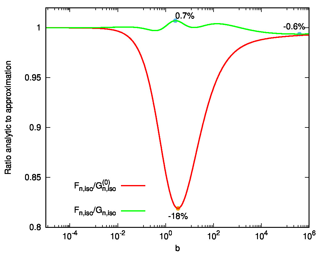
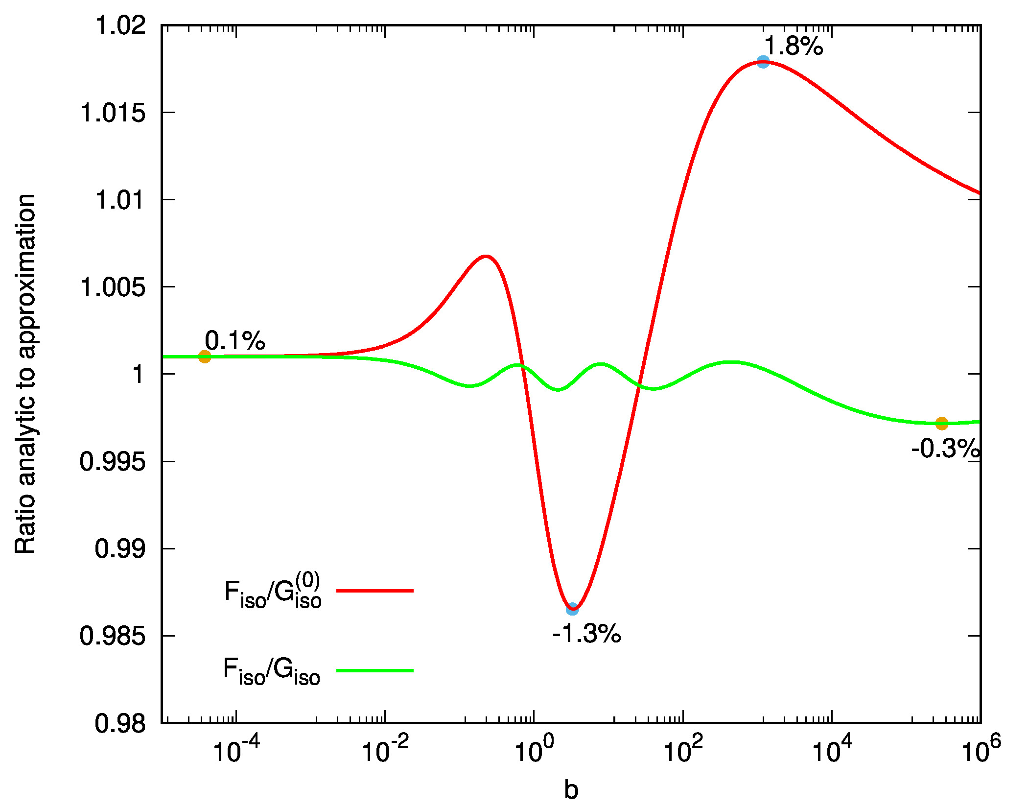
Figure 1: Top panel: The ratio of the function $F_{\mathrm{n,iso}}$ to $G_{\mathrm{n,iso}}^{(0)}$ and $F_{\mathrm{n,iso}}$ to $G_{\mathrm{n,iso}}^{(0)}\times g_{i}$(for $a_{i}=0.24$, $\alpha_{i}=0.89$, $b_{i}=0.4$, and $\beta_{i}=1.36$). Bottom panel: The ratio of the function $F_{\mathrm{iso}}$ to $G_{\mathrm{iso}}^{(0)}$ (for $c_{\mathrm{iso}}=0.785$) and $F_{\mathrm{iso}}$ to $G_{\rm iso}^{(0)}\times g_{i}$(for $c_{\mathrm{iso}}=0.87$, $a_{i}=-0.275$, $\alpha_{i}=1.02$, $b_{i}=4.24$, and $\beta_{i}=1.1$).

The mean photon energy can be obtained from the energy loss and scattering rates:

$$\bar{\omega}_{\mathrm{iso}}\quantity(E,\varepsilon)=\frac{\dot{E}_{\mathrm{iso}}}{\dot{N}_{\mathrm{iso}}}=E\frac{F_{\mathrm{iso}}(b)}{F_{\mathrm{n,iso}}(b)}\,.$$ (24)

In the Thomson and Klein-Nishina regimes, this yields the well-known asymptotic expressions

$$\frac{\bar{\omega}_{\mathrm{iso}}}{E}=\left\{\begin{matrix}b/3&\mbox{\quad if\quad}&b\ll 1\,,\\ 1&\mbox{\quad if\quad}&b\gg 1\,.\end{matrix}\right.$$ (25)

To express the mean photon energy in the transition regions, Eq. (24) can be approximated as

$$\frac{\bar{\omega}_{\mathrm{iso}}\quantity(E,\varepsilon)}{E}\approx\frac{G_{\mathrm{iso}}^{(0)}(b)}{G_{\mathrm{n,iso}}^{(0)}(b)}\,,$$ (26)

which can be further reduced to the simple expression,

$$\frac{\bar{\omega}_{\mathrm{iso}}\quantity(E,\varepsilon)}{E}\approx\frac{6b/5}{1+6b/5}\frac{\log\quantity(1+5b/27)}{\log\quantity(1+2b/3)}.$$ (27)

This provides a better than $2\%$ approximation for the upscattered photon energy in the entire energy range.

A similar expression is available for the anisotropic scattering regime. In this case, the asymptotic behavior is

$$\frac{\bar{\omega}_{\mathrm{ani}}}{E}=\left\{\begin{matrix}b_{\theta}/2&\mbox{\quad if\quad}&b_{\theta}\ll 1\,,\\ 1&\mbox{\quad if\quad}&b_{\theta}\gg 1\,.\end{matrix}\right.$$ (28)

If the scattering proceeds in the anisotropic regime, the following expression provides a better than $2\%$ approximation for the upscattered photon energy in the entire energy range

$$\frac{\bar{\omega}_{\mathrm{ani}}\quantity(E,\varepsilon)}{E}\approx\frac{2b_{\theta}}{1+2b_{\theta}}\frac{\log\quantity(1+b_{\theta}/2)}{\log\quantity(1+2b_{\theta})}\,.$$ (29)

3 $\delta$-function approximation

Both in the classical Thomson and quantum Klein-Nishina regimes, a monoenergetic distribution of electrons generates a broad IC component. If the electrons themselves feature a spread in their energy distribution, then the IC component is further broadened. Once the relative width of the electron distribution exceeds the relative width of single-electron IC spectrum, the width of the single-electron IC spectrum has little influence on the total IC component, and can thus be neglected. This can be appreciated by considering IC scattering under the $\delta$-function approximation. In this $\delta$-approximation treatment, the electron energy loss rate, $\dot{E}$, and mean frequency of IC photons generated by this electron, $\bar{\omega}$, determine the emission spectrum generated by the electron (see, e.g., 1966ApJ...146..686F; 2005ICRC....4..131K):

$$\dot{n}_{\gamma,0}=\absolutevalue{\frac{\dot{E}}{\omega}}\delta\quantity(\omega-\bar{\omega})\,,$$ (30)

where $\dot{n}_{\gamma,0}$ is the number of photons upscattered per unit time and frequency:

$$\dot{n}_{\gamma,0}=\derivative{\dot{N}_{\gamma,0}}{\omega}\,.$$ (31)

Equation (30) reproduces correctly the scattering rate and the radiation energy losses of the electrons emitted. The spectrum produced by an ensemble of electrons is obtained by convolution:

$$\dot{n}_{\gamma}=\int\differential{E}\dot{n}_{\gamma,0}n_{e}\,.$$ (32)

Here $n_{e}$ is electron energy distribution:

$$n_{e}=\derivative{N_{e}}{E}\,.$$ (33)

Although Eq. (30) and (32) can be considered an oversimplification, they still allow one to recover some basic properties of IC scattering, especially for the broadband part of the spectra far from either of the cutoff regions. For example, in the Thomson regime (see Eqs. (21) and (25)), the energy losses and the mean photon energy depend quadratically on energy: $\dot{E}\propto E^{2}$ and $\bar{\omega}\propto E^{2}$, respectively. If the electron distribution is a power law, $n_{e}\propto E^{-\alpha}$, then Eq. (32) yields the standard slope of the Thomson (or synchrotron) spectra (see, e.g., 2011hea..book.....L):

$$\dot{n}_{\gamma}\propto\omega^{-(\alpha+1)/2}\,.$$ (34)

In the Klein-Nishina regime, the energy loss rate is constant, $\dot{E}\propto\mathrm{const}$ (ignoring the logarithm dependence, see Eq. (21)), and the mean photon energy is $\bar{\omega}\propto E$, thus for the power-law distribution of electrons one obtains (see, e.g., in 1970RvMP...42..237B)

$$\dot{n}_{\gamma}\propto\omega^{-(\alpha+1)}\,.$$ (35)

If the distribution of the target photons is sufficiently broad, then the width target spectrum needs accounting for. This can also be addressed under the $\delta$-function approximation:

$$\dot{n}_{\gamma,0}=\int\frac{1}{\omega}\absolutevalue{\derivative{\dot{E}}{\varepsilon}}\delta\quantity(\omega-\bar{\omega}\quantity(E,\varepsilon))\differential{\varepsilon}\,,$$ (36)

where $\differential{\dot{E}}$ is the electron energy loss rate caused by the interaction with target photons that have their energy exclusively in the range from $\varepsilon$ to $\varepsilon+\differential{\varepsilon}$.

If the distribution of the target photons is sufficiently broad, then at least a fraction of the target photons is up scattered in the Thomson regime. Since the scattering cross-section in the Klein-Nishina regime is smaller than the Thomson cross-section, the part of the spectrum formed in the Thomson regime should reflect the key spectral properties. These features can be studied by setting $\bar{\omega}\propto\varepsilon E^{2}$ and $\differential{\dot{E}}/\differential{\varepsilon}\propto\varepsilon n_{\mathrm{ph}}(\varepsilon)E^{2}$, where $n_{\mathrm{ph}}$ is the energy distribution of the target photons. Thus, one obtains

$$\dot{n}_{\gamma}^{\mathrm{T}}\propto\int\differential{E}\int\differential{\varepsilon}\frac{1}{\omega}E^{2}\varepsilon n_{e}(E)n_{\mathrm{ph}}(\varepsilon)\delta\quantity(\omega-\frac{\varepsilon E^{2}}{m_{e}^{2}c^{4}})\,.$$ (37)

The integration over the $\delta$-function helps to clearly reveal the production of the broadband spectrum in the Thomson limit. Before writing the resulting equation, we note that given the presence of the $\delta$-function term, one does not need to account for the kinematic constraints on the energies of the interacting particles. However, to ensure that the scattering proceeds in the Thomson regime, we introduce a Heaviside function that determines the maximum frequency of the scattered photons: $\Theta\quantity(1-\varepsilon E/(m_{e}^{2}c^{4}))$ (note that in this section we omit some numerical factors, this, however, does not influence the conclusions). Thus, one obtains

$$\dot{n}_{\gamma}^{\mathrm{T}}\propto\int\differential{E}\frac{1}{E^{2}}n_{e}(E)n_{\mathrm{ph}}\quantity(\frac{\omega m_{e}^{2}c^{4}}{E^{2}})\Theta\quantity(E-\omega)=$$ (38)

$$\int\limits_{\omega}^{\infty}\differential{E}\frac{1}{E^{2}}n_{e}(E)n_{\mathrm{ph}}\quantity(\frac{\omega m_{e}^{2}c^{4}}{E^{2}})\,,$$

where the lower energy limit in the integral is due to the Heaviside function, i.e., it is imposed by the Klein-Nishina cutoff, which, according to the assumptions introduced, is equivalent to an obvious requirement, $E>\omega$.

Let us assume that one deals with a power-law distributions of electrons and target photons:

$$n_{e}\propto E^{-\alpha}\Theta\quantity(E-E_{\mathrm{min}})\Theta\quantity(E_{\mathrm{max}}-E)$$ (39)

and

$$n_{\mathrm{ph}}\propto\varepsilon^{-\beta}\Theta\quantity(\varepsilon-\varepsilon_{\mathrm{min}})\Theta\quantity(\varepsilon_{\mathrm{max}}-\varepsilon)\,.$$ (40)

Provided that $E_{\mathrm{max}}>m_{e}c^{2}\sqrt{\omega/\varepsilon_{\mathrm{max}}}$ and $E_{\mathrm{min}}<m_{e}c^{2}\sqrt{\omega/\varepsilon_{\mathrm{min}}}$, the integral in Eq. (38) is a simple power-law function:

$$\dot{n}_{\gamma}^{\mathrm{T}}\propto\omega^{-\beta}\int\limits_{\tilde{E}_{\mathrm{min}}}^{\tilde{E}_{\mathrm{max}}}\differential{E}E^{2\beta-\alpha-2}\,,$$ (41)

where the integral limits are determined by the following conditions

$$\tilde{E}_{\mathrm{min}}=\max\quantity(\omega,E_{\mathrm{min}},m_{e}c^{2}\sqrt{\frac{\omega}{\varepsilon_{\mathrm{max}}}})$$ (42)

and

$$\tilde{E}_{\mathrm{max}}=\min\quantity(E_{\mathrm{max}},m_{e}c^{2}\sqrt{\frac{\omega}{\varepsilon_{\mathrm{min}}}})\,.$$ (43)

Provided $2\beta-\alpha\neq 1$ the final expression is

$$\dot{n}_{\gamma}^{\mathrm{T}}\propto\omega^{-\beta}\frac{1}{2\beta-\alpha-1}\quantity(\tilde{E}^{2\beta-\alpha-1}_{\mathrm{max}}-\tilde{E}^{2\beta-\alpha-1}_{\mathrm{min}})\,,$$ (44)

where the leading term is determined by the sign of the exponent, $2\beta-\alpha-1$.

If the sign of this exponent is positive, i.e. $\alpha<2\beta-1$, then the resulting spectrum is approximately

$$\dot{n}_{\gamma}^{\mathrm{T}}\propto\left\{\begin{matrix}\omega^{-(\alpha+1)/2}&\mbox{\quad if\quad}\omega<\frac{\varepsilon_{\mathrm{min}}E_{\mathrm{max}}^{2}}{m_{e}^{2}c^{4}}\,,\\ \omega^{-\beta}&\mbox{\quad if\quad}\omega>\frac{\varepsilon_{\mathrm{min}}E_{\mathrm{max}}^{2}}{m_{e}^{2}c^{4}}\,.\\ \end{matrix}\right.$$ (45)

Thus, it can be seen that the spectrum keeps the same slope as that predicted by the standard Thomson estimate. If the IC spectrum extends into the energy range where the lower energy part of the spectrum doesn’t make any contribution, $\omega>\varepsilon_{\mathrm{min}}E_{\mathrm{max}}^{2}/(m_{e}^{2}c^{4})$, the IC spectrum is determined by the slope of the target photons, $\dot{n}_{\gamma}^{\mathrm{T}}\propto\omega^{-\beta}$. The relation between the parameters is graphically shown in Fig. 2.

A similar effect defines the slope of the low-energy part of the IC spectrum if $\alpha>2\beta-1$. In this case, the high-energy part of the target photon spectrum provides the most important contribution, and the slope of IC emission is inherited from the target photon spectrum if $\omega<\varepsilon_{\mathrm{max}}E_{\mathrm{min}}^{2}/(m_{e}^{2}c^{4})$ and $\omega<E_{\mathrm{min}}$. The dependence of $\tilde{E}_{\mathrm{min}}$ on $\omega$ is sketched out in Fig. 3. If $E_{\mathrm{min}}>m_{e}^{2}c^{4}/\varepsilon_{\mathrm{max}}$ the IC spectrum directly translates from $\omega^{-\beta}$ to $\omega^{-\alpha+\beta-1}$ at $\omega=E_{\mathrm{min}}$. If $E_{\mathrm{min}}<m_{e}^{2}c^{4}/\varepsilon_{\mathrm{max}}$ the transition between these two regimes proceeds through $\omega^{-(\alpha+1)/2}$, which is realized for $\varepsilon_{\mathrm{max}}E_{\mathrm{min}}^{2}/(m_{e}^{2}c^{4})<\omega<m_{e}^{2}c^{4}/\varepsilon_{\mathrm{max}}$. These spectral properties are summarized by the following expressions (see also Fig. 3):

$$\dot{n}_{\gamma}^{\mathrm{T}}\propto\left\{\begin{matrix}\omega^{-\beta}&\mbox{\quad if\quad}&\omega<\frac{\varepsilon_{\mathrm{max}}E_{\mathrm{min}}^{2}}{m_{e}^{2}c^{4}}&\mbox{\quad and\quad}&\omega<E_{\mathrm{min}}\,,\\ \omega^{-(\alpha+1)/2}&\mbox{\quad if\quad}&\omega>\frac{\varepsilon_{\mathrm{max}}E_{\mathrm{min}}^{2}}{m_{e}^{2}c^{4}}&\mbox{\quad and\quad}&\omega<\frac{m_{e}^{2}c^{4}}{\varepsilon_{\mathrm{max}}}\,,\\ \omega^{-(\alpha+1)+\beta}&\mbox{\quad if\quad}&\omega>E_{\mathrm{min}}&\mbox{\quad and\quad}&\omega>\frac{m_{e}^{2}c^{4}}{\varepsilon_{\mathrm{max}}}\,.\end{matrix}\right.$$ (46)

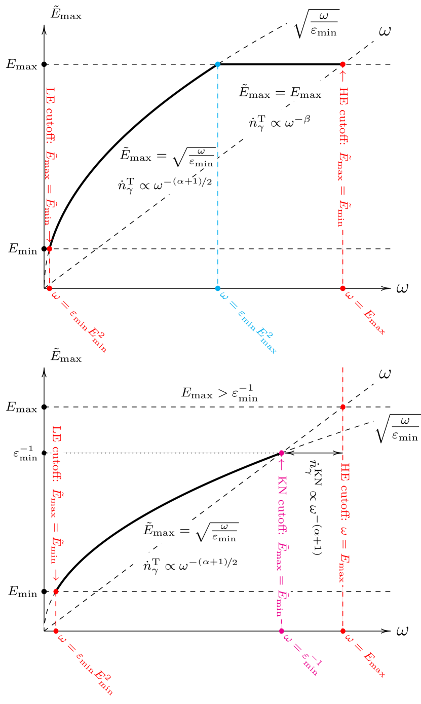
Figure 2: Dependence of $\tilde{E}_{\mathrm{max}}$ from Eq. (43) on the upscattered photon energy together with the conditions that determine the cutoff energy. Note that in the figure labels we omit $m_{e}c^{2}$ factors.

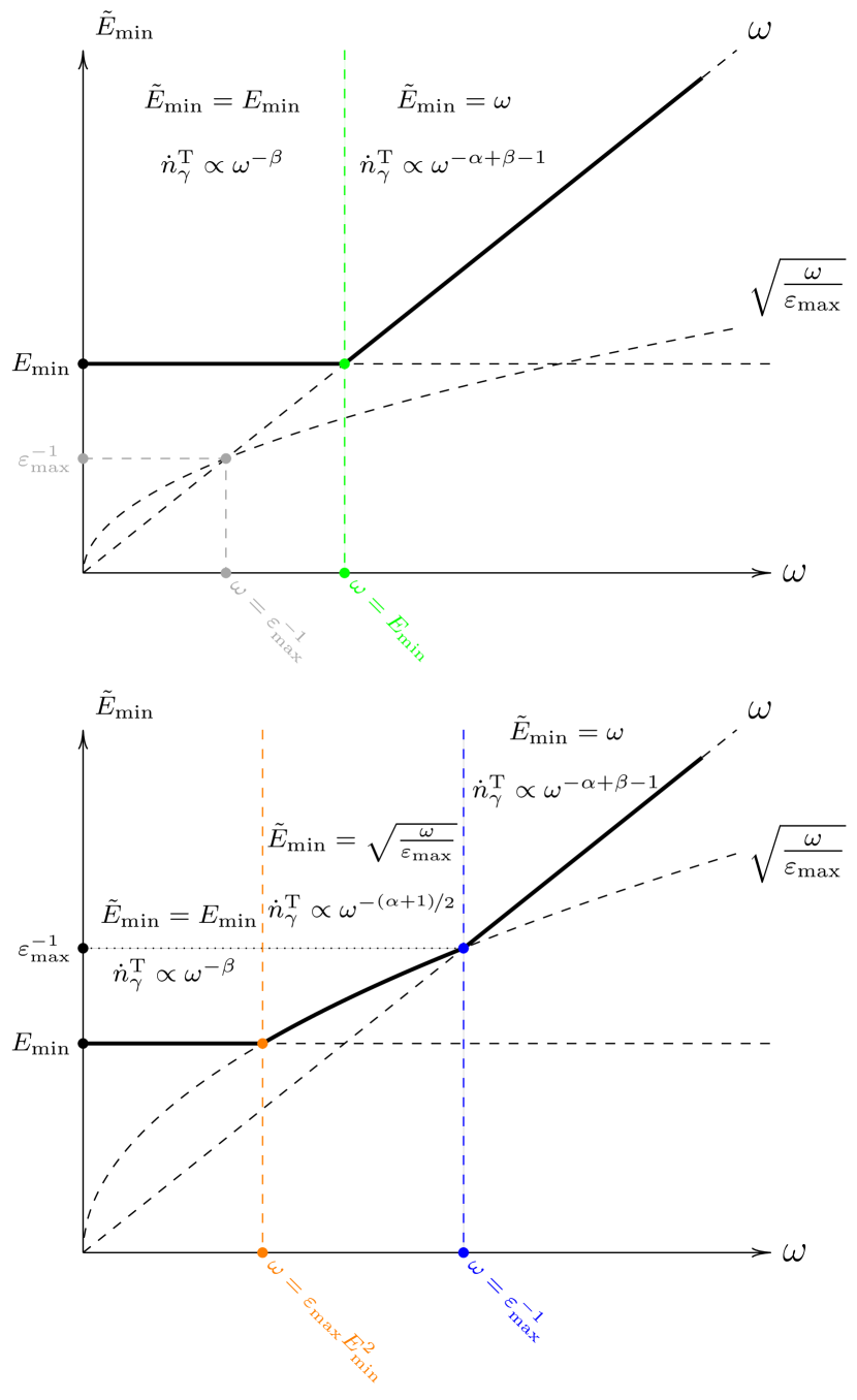
Figure 3: Dependence of $\tilde{E}_{\mathrm{min}}$ from Eq. (42) on the upscattered photon energy. Note that in the figure labels we omit $m_{e}c^{2}$ factors.

The resultant IC spectra obtained by numerical integration of the differential cross-section over power-law distributions of target photons and electrons are shown in Figs. 4 and 5. The simple analytic dependencies shown in the figures are given by Eqs. (45) and (46). Also, it can be seen from Fig. 5 that Eq. (35) describes the spectral slope in the part of the spectrum generated in the Klein-Nishina regime.

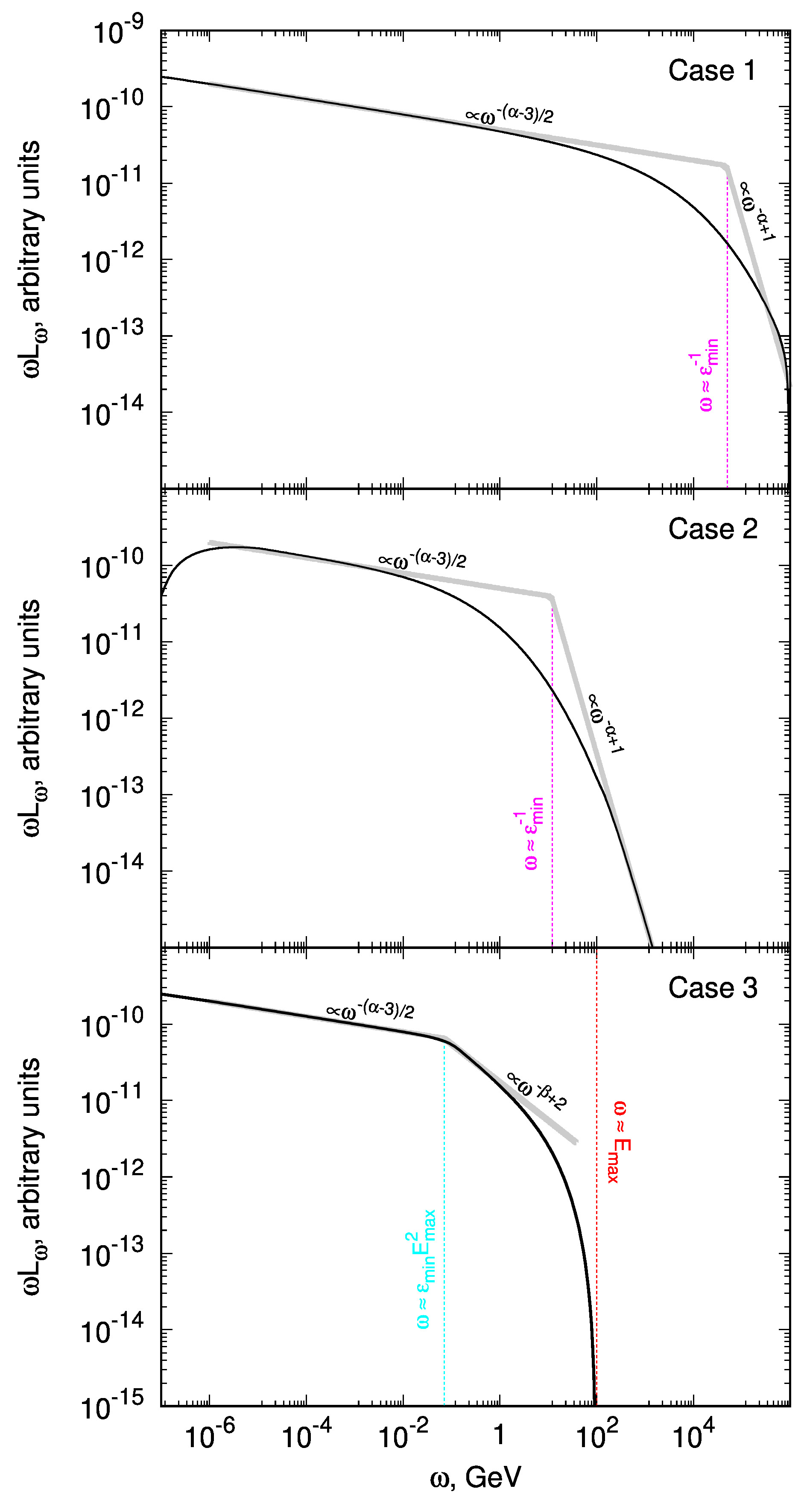
Figure 4: Numerical computation of IC spectrum produced on a power-law target photons with $\beta=2.5$. Upper panel (“Case 1”): minimum and maximum energies of target photons are $\varepsilon_{\mathrm{min}}=10^{-3}\,\mathrm{eV}$ and $\varepsilon_{\mathrm{max}}=1\,\mathrm{keV}$, respectively; the electron maximum energy was set to $E_{\mathrm{max}}=1\,\mathrm{PeV}$. Middle panel (“Case 2”): minimum and maximum energies of target photons are $\varepsilon_{\mathrm{min}}=10\,\mathrm{eV}$ and $\varepsilon_{\mathrm{max}}=3\,\mathrm{keV}$, respectively; the electron maximum energy was set to $E_{\mathrm{max}}=1\,\mathrm{PeV}$. Bottom panel (“Case 3”): minimum and maximum energies of target photons are $\varepsilon_{\mathrm{min}}=10^{-3}\,\mathrm{eV}$ and $\varepsilon_{\mathrm{max}}=1\,\mathrm{keV}$, respectively; the electron maximum energy was set to $E_{\mathrm{max}}=100\,\mathrm{GeV}$. The electron energy distribution was assumed to be a power law with $\alpha=3.2$ above $E_{\mathrm{min}}=1\,\mathrm{MeV}$. The solid guide lines indicate the analytic slopes expected from Eq. (45) and (35) (in the Klein-Nishina limit) and the dashed guide lines indicate the positions of spectral transformations given by Eqs. (45) and (49). The slope labels show the energy flux spectral indices.

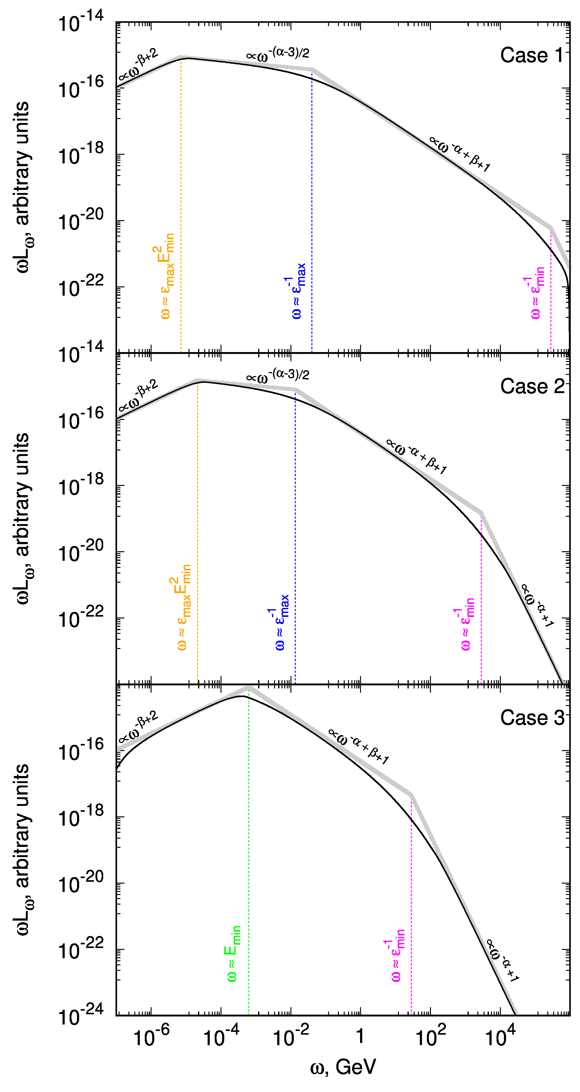
Figure 5: Numerical computation of IC spectrum produced on a power-law target photons with $\beta=1.5$. Upper panel (“Case 1”): minimum and maximum energies of target photons are $\varepsilon_{\mathrm{min}}=10^{-3}\,\mathrm{eV}$ and $\varepsilon_{\mathrm{max}}=1\,\mathrm{keV}$, respectively. Middle panel (“Case 2”): minimum and maximum energies of target photons are $\varepsilon_{\mathrm{min}}=10^{-1}\,\mathrm{eV}$ and $\varepsilon_{\mathrm{max}}=3\,\mathrm{keV}$, respectively. Bottom panel (“Case 3”): minimum and maximum energies of target photons are $\varepsilon_{\mathrm{min}}=10\,\mathrm{eV}$ and $\varepsilon_{\mathrm{max}}=100\,\mathrm{keV}$, respectively. The electron energy distribution was assumed to be a power law with $\alpha=3.2$ between $E_{\mathrm{min}}=1\,\mathrm{MeV}$ and $E_{\mathrm{max}}=1\,\mathrm{PeV}$. The solid guide lines shown are the analytic slopes expected from Eqs. (46) and (35) (in the Klein-Nishina limit) and dashed guide lines indicate the positions of spectral transformations given by Eqs. (46) and (49). The slope labels show the energy flux spectral indices.

Another important question is in which energy interval the revealed power-law dependencies are relevant. The approach used is relevant if the integration interval is sufficiently broad. Thus, the condition of the applicability of the obtained results is

$$\tilde{E}_{\mathrm{min}}\ll\tilde{E}_{\mathrm{max}}\,.$$ (47)

Once the integral limits approach each other, the power-law behavior becomes distorted, and the integral in Eq. (41) starts to vanish, i.e., the condition $\tilde{E}_{\mathrm{min}}\sim\tilde{E}_{\mathrm{max}}$ defines the position of the spectral cutoffs. The low-energy cutoff is then simply given by the condition

$$\omega_{\mathrm{min}}\approx\frac{\varepsilon_{\mathrm{min}}E_{\mathrm{min}}^{2}}{m_{e}^{2}c^{4}}\,.$$ (48)

For the high-energy cutoff, the determination of the conditions is a little more involved. Unless the parameters are tuned, it is natural to expect that in the high $\omega$ regime the low energy limit of the integral, Eq. (42), is simply $\omega$. The upper bound can be either $E_{\mathrm{max}}$ or $m_{e}c^{2}\sqrt{\frac{\omega}{\varepsilon_{\mathrm{min}}}}$ (see in Fig. 2 for a sketch). In the former case, the disappearance of the integral is caused by $\omega\rightarrow E_{\mathrm{max}}$ and the spectrum should completely disappear at $E_{\mathrm{max}}$. This is shown by the IC spectrum computed for $E_{\mathrm{max}}=100\,\mathrm{GeV}$ in the bottom panel of Fig. 4.

In the case when $E_{\mathrm{max}}>m_{e}^{2}c^{4}/\varepsilon_{\mathrm{min}}$, one should expect a transition to the Klein-Nishina regime when $\omega\rightarrow m_{e}c^{2}\sqrt{\frac{\omega}{\varepsilon_{\mathrm{min}}}}$. This means that at the gamma-ray energy

$$\omega_{\mathrm{kn}}\sim\frac{m_{e}^{2}c^{4}}{\varepsilon_{\mathrm{min}}}\,,$$ (49)

the IC spectrum should obtain a typical slope for the Klein-Nishina regime: $\dot{n}_{\gamma}\propto\omega^{-(\alpha+1)}$ (see in Fig. 2). This transformation is illustrated by curves computed for $\varepsilon_{\mathrm{min}}=10\,\mathrm{eV}$ in Figs. 4 and 5.

However, we note that the IC spectra can appear significantly harder than that expected to be produced via interactions in the Klein-Nishina regime, if the distribution of target photons extends to sufficiently low energies (i.e., the condition given by Eq. (49) is not fulfilled — see the spectra computed for $\varepsilon_{\mathrm{min}}=10^{-3}\,\mathrm{eV}$ in the top panels of Figs. 4 and 5).

So far, we have assumed that $\beta\neq(\alpha+1)/2$. However, this specific case deserves special mention as synchrotron emission produced by electrons having a power-law energy distribution gives rise to a power-law spectrum with photon index $(\alpha+1)/2$. In this case, all the revealed photon indexes of the IC component generated in the Thomson regime correspond to the same spectral slope, as one has

$$\frac{\alpha +1}{2}=$$ (50)