Anomalous Dimensions at an Infrared Fixed Point in an SU($N_{c}$) Gauge Theory with Fermions in the Fundamental and Antisymmetric Tensor Representations

Abstract

We present scheme-independent calculations of the anomalous dimensions $\gamma_{\bar{\psi}\psi,IR}$ and $\gamma_{\bar{\chi}\chi,IR}$ of fermion bilinear operators $\bar{\psi}\psi$ and $\bar{\chi}\chi$ at an infrared fixed point in an asymptotically free SU($N_{c}$) gauge theory with massless Dirac fermion content consisting of $N_{F}$ fermions $\psi^{a}_{i}$ in the fundamental representation and $N_{A_{2}}$ fermions $\chi^{ab}_{j}$ in the antisymmetric rank-2 tensor representation, where $i,j$ are flavor indices. For the case $N_{c}=4$, $N_{F}=4$, and $N_{A_{2}}=4$, we compare our results with values of these anomalous dimensions measured in a recent lattice simulation and find agreement.

I Introduction

An asymptotically free gauge theory with sufficiently many massless fermions has an infrared zero in its beta function, which is an infrared fixed point (IRFP) of the renormalization group b1 ; b2 ; bz . At this IRFP the theory is scale-invariant and is inferred to be conformally invariant scalecon , whence the commonly used term “conformal window” (CW). Because of the asymptotic freedom, one can use perturbation theory reliably in the deep ultraviolet (UV) where the gauge coupling approaches zero, and then follow the renormalization-group flow toward the infrared. These statements apply to both vectorial and chiral gauge theories; here we restrict our consideration to vectorial gauge theories. As the fermion content is reduced, the gauge coupling at the IRFP increases in strength and eventually exceeds a value such that there is generically spontaneous chiral symmetry breaking and dynamical fermion mass generation. This defines the lower end of the conformal window. Theories that lie slightly below this lower end exhibit quasi-conformal behavior over a large interval of Euclidean energy/momentum scales, over which the gauge coupling runs slowly due to a small beta function. Such theories just below the lower end of the conformal window can be relevant to approaches to composite-Higgs scenarios and associated physics beyond the Standard Model (BSM). Considerable progress has been made in studies of quasi-conformal vectorial gauge theories with several flavors of fermions transforming according to a single representation of the gauge group, e.g., SU(3) with $N_{F}=8$ Dirac fermions in the fundamental representation lsd_2016 -lsd_2019 .

For an operator ${\cal O}$, the full scaling dimension is denoted as $D_{\cal O}$ and its free-field value as $D_{{\cal O},free}$. The anomalous dimension of this operator, denoted $\gamma_{\cal O}$, is defined via the relation $D_{\cal O}=D_{{\cal O},free}-\gamma_{\cal O}$. The anomalous dimensions of gauge-invariant operators at an IRFP are of basic physical interest. While the simplest gauge theories have used fermions transforming according to a single representation of the gauge group, a natural generalization is to study theories with multiple fermions transforming according to different representations of the gauge group. In previous work dexm , we presented scheme-independent perturbative calculations of anomalous dimensions of fermion bilinears at an IRFP in the conformal window in a theory of this type (in $d=4$ spacetime dimensions at zero temperature), with a general non-Abelian gauge group $G$ and massless fermion content consisting of $N_{f}$ fermions $f$ in a representation $R$ and $N_{f^{\prime}}$ fermions $f^{\prime}$ in a representation $R^{\prime}$ of $G$ fm . Our calculational method applies at an exact IRFP in the conformal window (sometimes called the non-Abelian Coulomb phase). In dexml with S. Girmohanta we studied theories of this type with $G={\rm SU}(N_{c})$, $R$ equal to the fundamental representation, and $R^{\prime}$ equal to the adjoint or rank-2 tensor representation and investigated a type of ’t Hooft-Veneziano limit, $N_{f}\to\infty$, $N_{c}\to\infty$ with $N_{f}/N_{c}$ and $N_{f^{\prime}}$ fixed.

We denote a gauge theory with gauge group $G={\rm SU}(N_{c})$ and (massless) fermion content consisting of $N_{F}$ Dirac fermions in the fundamental representation, denoted $F$, and $N_{A_{2}}$ Dirac fermions in the antisymmetric rank-2 tensor representation, denoted $A_{2}$, as $(N_{c},N_{F},N_{A_{2}})$ for short. Recently, Ref. fx444 has reported interesting results from lattice simulations of the $(N_{c},N_{F},N_{A_{2}})=(4,4,4)$ theory. Since the $A_{2}$ representation in SU(4) is self-conjugate, the $N_{A_{2}}$ Dirac fermions are equivalent to $2N_{A_{2}}$ Majorana fermions. Ref. fx444 finds evidence for an IRFP inferred to lie in the conformal window, near its lower end, and presents measurements of the anomalous dimensions of the $F$ and $A_{2}$ fermion bilinears $\gamma^{(4)}_{m}$ and $\gamma^{(6)}_{m}$ (where the superscripts refer to the dimensionalities of these representations of SU(4)), and of gauge-singlet composite-fermion operators. Given the conclusion in fx444 that this theory is in the conformal window, a relevant question is whether our general higher-order perturbative calculations of anomalous dimensions of fermion bilinears in dexm , when specialized to this theory, yield results in agreement with the values measured in fx444 . To our knowledge, this question has not been previously investigated in the literature.

In the present work we address and answer this question for the anomalous dimensions $\gamma^{(4)}_{m}$ and $\gamma^{(6)}_{m}$ by extracting the requisite special case of our general calculations of anomalous dimensions of fermion bilinears in dexm for the $(N_{c},N_{F},N_{A_{2}})=(4,4,4)$ theory. To state our conclusions in advance, to within the uncertainties in our finite-order perturbative calculation, we find agreement with the lattice results in fx444 . The authors of Ref. fx444 also observed that their conclusion that the (4,4,4) theory is in the conformal window disagreed with a calculation in khl (denoted KHL) of the lower boundary of this conformal window in the $(4,N_{F},N_{A_{2}})$ theory based on a critical condition on ${\rm max}(\gamma_{m}^{(4)},\ \gamma_{m}^{(6)})$, denoted $\gamma$CC. We investigate this further here.

As noted above, our calculations of anomalous dimensions of fermion bilinears in dexm were for a general non-Abelian gauge group $G$ and fermion representations $R$ and $R^{\prime}$. Before presenting our calculations for SU(4) theory, we will first specialize the results from dexm to the case of the gauge group $G={\rm SU}(N_{c})$ with massless fermion content consisting of $N_{F}$ Dirac fermions in the fundamental representation and $N_{A_{2}}$ Dirac fermions in the antisymmetric rank-2 tensor representation of SU($N_{c}$), i.e., theories of the type $(N_{c},N_{F},N_{A_{2}})$ in our shorthand notation. We then further specialize to the case $N_{c}=4$, and then finally to the $(4,4,4)$ theory.

We denote the massless Dirac fermions in the $F$ and $A_{2}$ representations as $\psi^{a}_{i}$ and $\chi^{ab}_{j}=-\chi^{ba}_{j}$, where $a,b$ are SU($N_{c}$) gauge indices, and $i,j$ are flavor indices with $i=1,...,N_{F}$ and $j=1,...,N_{A_{2}}$. We shall use our general results in dexm to calculate scheme-independent series expansions for the anomalous dimensions at the IRFP, denoted $\gamma_{\bar{\psi}\psi,IR}$ and $\gamma_{\bar{\chi}\chi,IR}$, of the respective (gauge-invariant) fermion bilinears

$$\bar{\psi}\psi=\sum_{i=1}^{N_{f}}\bar{\psi}_{a,i}\psi^{a}_{i}$$ (1)

and

$$\bar{\chi}\chi=\sum_{j=1}^{N_{A_{2}}}\bar{\chi}_{ab,j}\chi^{ab}_{j}\ ,$$ (2)

where the sums over color indices are understood and run from 1 to $N_{c}$. Although we take the fermions to be massless, the operators (1) and (2) would be mass operators (with all fermion flavors taken to have equal mass) if these fermions were massive, and for this reason another common notation for the anomalous dimensions is $\gamma^{(F)}_{m}\equiv\gamma_{\bar{\psi}\psi,IR}$ and $\gamma^{(A_{2})}_{m}\equiv\gamma_{\bar{\chi}\chi,IR}$. In the special case $N_{c}=4$, these are also written with reference to the respective dimensionalities 4 and 6 of the $F$ and $A_{2}$ representations as $\gamma^{(4)}_{m}\equiv\gamma_{\bar{\psi}\psi,IR}$ and $\gamma^{(6)}_{m}\equiv\gamma_{\bar{\chi}\chi,IR}$. The color and flavor indices will often be suppressed in the notation.

It should be mentioned that studies were also performed of the (4,2,2) theory, due to its possible role as a model for a composite Higgs boson and a partially composite top quark degrand_etal -deldebbio . However, as we noted in dexm , the (4,2,2) theory is in the chirally broken phase, where there is no exact IRFP and hence where our calculations are not directly applicable. In general, BSM theories with fermions in higher-dimensional representations have long been of interest; in addition to Refs. fx444 and degrand_etal -deldebbio , some of the many works include higherrep ; sextet ; ferretti .

This paper is organized as follows. In Section II we briefly discuss some relevant background and our general calculational methods. Section III contains our results for the anomalous dimensions for SU($N_{c}$) with general $N_{F}$ and $N_{A_{2}}$ in the conformal window, while Section IV presents the corresponding formulas for $N_{c}=4$ and for the specific $(N_{c},N_{F},N_{A_{2}})=(4,4,4)$ theory. Our conclusions are given in Section V.

II Calculational Methods

In this section we briefly review our calculational methods and relevant notation. In the context of the general SU($N_{c}$) gauge group, we first mention two degenerate cases. If $N_{c}=2$, then the $A_{2}$ representation is a singlet and hence decouples from the dynamics, so the theory reduces to one with fermions in just the fundamental representation. Hence, in all expressions involving the number $N_{A_{2}}$, this number always occurs multipled by the factor $(N_{c}-2)$. If $N_{c}=3$, then $A_{2}=\bar{F}$, i.e., the $A_{2}$ representation is the conjugate fundamental representation of SU(3). Taking into account the fact that a Dirac fermion $f$ has a decomposition into chiral components $f=f_{L}+f_{R}$ and the property that a left-handed chiral component of a fermion can be equivalently written as the charge conjugate of a right-handed antifermion, it follows that if $N_{c}=3$, then the theory reduces to one with $N_{F}+N_{A_{2}}$ fermions in the fundamental representation. If $N_{c}\geq 4$, then the $F$ and $A_{2}$ representations are distinct.

II.1 Relevant Range of $N_{F}$ and $N_{A_{2}}$

We denote the running gauge coupling as $g=g(\mu)$, where $\mu$ is the Euclidean energy/momentum scale at which this coupling is measured. We define $\alpha(\mu)=g(\mu)^{2}/(4\pi)$. As noted before, since we require the theory to be asymptotically free, its properties can be computed perturbatively in the UV limit at large $\mu$, where $\alpha(\mu)\to 0$. The dependence of $\alpha(\mu)$ on $\mu$ is described by the renormalization-group (RG) beta function,

$$\beta=\frac{d\alpha(\mu)}{d\ln\mu}\ .$$ (3)

The argument $\mu$ will generally be suppressed in the notation. The series expansion of $\beta$ in powers of $\alpha$ is

$$\beta=-2\alpha\sum_{\ell=1}^{\infty}b_{\ell}\,a^{\ell}\ ,$$ (4)

where

$$a\equiv\frac{g^{2}}{16\pi^{2}}=\frac{\alpha}{4\pi}\ ,$$ (5)

and $b_{\ell}$ is the $\ell$-loop coefficient. For a theory with a gauge group $G$ and Dirac fermions $f$ and $f^{\prime}$ in respective representations $R$ and $R^{\prime}$ of $G$, the one-loop coefficient in the beta function is b1

$$b_{1}=\frac{1}{3}\Big{[}11C_{A}-4(N_{f}T_{f}+N_{f^{\prime}}T_{f^{\prime}})\Big{]}\ ,$$ (6)

and the two-loop coefficient is b2

$$b_{2}=\frac{1}{3}\bigg{[}34C_{A}^{2}-4N_{f}T_{f}(5C_{A}+3C_{f})-4N_{f^{\prime}}T_{f^{\prime}}(5C_{A}+3C_{f^{\prime}})\bigg{]}\ ,$$ (7)

where $C_{A}$, $C_{f}$, and $T_{f}$ are group invariants (see rsv and the Appendix). With an overall minus sign extracted, as in Eq. (3), the condition of asymptotic freedom is that $b_{1}>0$. Setting $R=F$ and $R^{\prime}=A_{2}$ and substituting the values of the group invariants for $G={\rm SU}(N_{c})$, the condition $b_{1}>0$ reads

$$N_{F}+(N_{c}-2)N_{A_{2}}<\frac{11N_{c}}{2}\ .$$ (8)

The resultant upper ($u$) limits on $N_{F}$ and $N_{A_{2}}$ imposed by the requirement of asymptotic freedom are thus

$$N_{F,u}=\frac{11}{2}N_{c}-(N_{c}-2)N_{A_{2}}$$ (9)

and

$$N_{A_{2},u}=\frac{11N_{c}-2N_{F}}{2(N_{c}-2)}\ .$$ (10)

The maximal order to which the beta function is independent of the scheme used for regularization and renormalization is the two-loop order. With $b_{1}>0$, the condition that this two-loop beta function should have an IR zero is that $b_{2}<0$. For the SU($N_{c}$) theory, this is the condition

$$N_{F}(13N_{c}^{2}-3)+2N_{A_{2}}(N_{c}-2)(8N_{c}^{2}-3N_{c}-6)>34N_{c}^{3}\ .$$ (11)

The region of the first quadrant in the $(N_{F},N_{A_{2}})$ plane where the inequalities (8) and (11) are both satisfied will be denoted $I_{IRZ}$, where the subscript refers to the existence of an IR zero (IRZ) in the beta function. We label the upper and lower boundaries of the $I_{IRZ}$ region as ${\cal B}_{IRZ,u}$ and ${\cal B}_{IRZ,\ell}$, respectively. In plotting these boundaries, one formally generalizes $N_{F}$ and $N_{A_{2}}$ from positive integers (or half-integers for $N_{A_{2}}$ if $N_{c}=4$) to positive real numbers, with the understanding that the physical cases are integral (or half-integral for $N_{A_{2}}$ if $N_{c}=4$). Analogously, we denote the upper and lower boundaries of the conformal window as ${\cal B}_{CW,u}$ and ${\cal B}_{CW,\ell}$, respectively. The upper boundary ${\cal B}_{CW,u}={\cal B}_{IRZ,u}$ is the solution locus to the condition $b_{1}=0$. The lower boundary ${\cal B}_{CW,\ell}$ is not exactly known even for the case of theories with fermions transforming in only one representation; indeed, much work using lattice simulations has been, and continues to be, devoted to determining the approximate location of this lower conformal-window boundary lgtreviews ; simons . We discuss this lower boundary ${\cal B}_{CW,\ell}$ further below for the $N_{c}=4$ theory.

Following our labelling convention in dexm , we take the horizontal and vertical axes of the first quadrant of the $(N_{F},N_{A_{2}})$ plane to be the $N_{F}$ and $N_{A_{2}}$ axes, respectively. The boundaries of the $I_{IRZ}$ region given by the equations $b_{1}=0$ and $b_{2}=0$ are both line segments in this first quadrant of the $(N_{F},N_{A_{2}})$ plane. In general, the slope of the line $b_{1}=0$ is

$$\frac{dN_{A_{2}}}{dN_{F}}=-\frac{1}{N_{c}-2}\ ,$$ (12)

and the slope of the line $b_{2}=0$ is

$$\frac{dN_{A_{2}}}{dN_{F}}=-\frac{(13N_{c}^{2}-3)}{2(N_{c}-2)(8N_{c}^{2}-3N_{c}-6)}\ .$$ (13)

II.2 Higher-Order Terms in Beta Function

For a theory with a general gauge group $G$ and $N_{f}$ fermions in a single representation, $R$, the coefficients $b_{1}$ and $b_{2}$ were calculated in b1 and b2 , while $b_{3}$, $b_{4}$, and $b_{5}$ were calculated in the commonly used $\overline{\rm MS}$ scheme msbar in b3a ; b3b , b4 , and b5 , respectively (see also b5su3 ). For the analysis of a theory with fermions in multiple different representations, one needs generalizations of these results. These are straightforward to derive in the case of $b_{1}$ and $b_{2}$, but new calculations are required for higher-loop coefficients. These were performed in zoller (again in the $\overline{\rm MS}$ scheme) up to four-loop order, and we used the results of Ref. zoller in dexm .

II.3 Anomalous Dimensions

The conventional expansion of the anomalous dimension $\gamma_{\bar{f}f}$ of the fermion bilinear $\bar{f}f$ in a gauge theory, in terms of the squared gauge coupling, is

$$\gamma_{\bar{f}f}=\sum_{\ell=1}^{\infty}c^{(f)}_{\ell}\,a^{\ell}\ ,$$ (14)

where $c^{(f)}_{\ell}$ is the $\ell$-loop coefficient, and correspondingly for $\gamma_{\bar{f^{\prime}},f^{\prime}}$ in a theory with both $f$ and $f^{\prime}$ fermions. These expansions apply, in particular, at an IRFP. They may also be useful in the analysis of a quasi-conformal field theory with parameters such that it lies slightly below the lower end of the conformal window and hence exhibits UV to IR evolution over an extended interval of $\mu$ governed by an approximate IRFP. The one-loop coefficient $c^{(f)}_{1}$ is scheme-independent, while the $c^{(f)}_{\ell}$ with $\ell\geq 2$ are scheme-dependent, and similarly with the $c^{(f^{\prime})}_{\ell}$. For a general gauge group $G$ and $N_{f}$ fermions in a single representation $R$ of $G$, the $c^{(f)}_{\ell}$ have been calculated up to loop order $\ell=4$ in c4a ; c4b and $\ell=5$ in c5 . For the case of multiple fermion representations, the coefficients $c^{(f)}_{\ell}$ have been calculated up to four-loop order in chetzol in the $\overline{\rm MS}$ scheme.

Physical quantities such as anomalous dimensions at an IRFP clearly must be scheme-independent. In conventional computations of these quantities, one first writes them as series expansions in powers of the coupling as in (14), and then evaluates these series expansions with $\alpha$ set equal to $\alpha_{IR}$, calculated to a given loop order. These calculations have been performed for anomalous dimensions of gauge-invariant fermion bilinears in a theory with a single fermion representation up to the four-loop level bvh -bc and to the five-loop level in flir . However, as is well known, these conventional (finite-order) series expansions are scheme-dependent beyond the leading terms. Studies of scheme dependence in the context of an IRFP have been carried out in sch -schemegauge . The fact that the conventional series expansions for physical properties are scheme-dependent does not, by itself, reduce the usefulness of these expansions. For example, this scheme dependence is also true of higher-order calculations in quantum chromodynamics (QCD), which were used to analyze data from hadron colliders such as the Tevatron at Fermilab and the Large Hadron Collider at CERN. Considerable effort has been, and continues to be, expended to construct and apply schemes that minimize higher-order contributions in these QCD calculations brodsky . Indeed, in QCD, because the RG fixed point is an ultraviolet fixed point at the origin in coupling constant space, it is, in principle, possible to transform to a scheme where the beta function has no terms higher than two-loop order (the ’t Hooft scheme) hooft77 . However, as was shown in sch ; sch23 , it is considerably more difficult to try to carry out such a scheme transformation to remove terms at loop order 3 and higher for a fixed point away from the origin.

Thus, in the analysis of the properties of a theory at a fixed point away from the origin, as in the case of the IRFP of interest here, it is useful to employ a series expansion method for calculating physical quantities, such as anomalous dimensions, with the property that the results to each order are scheme-independent. A simple fact makes this possible: at the upper end of the conformal window, as $b_{1}\to 0$, this implies that $\alpha_{IR}\to 0$. Hence, one can reexpress a series expansion at an IRFP in the conformal window as an expansion in the manifestly scheme-independent variable $b_{1}$. For a theory with fermions $f$ in a single representation, it is natural to use the scheme-independent Banks-Zaks variable bz ; gkgg $\Delta_{f}=N_{f,u}-N_{f}$. Such calculations were carried out in gtr -baryon .

In dexm we generalized this analysis to theories with fermions $f$ and $f^{\prime}$ in different representations $R$ and $R^{\prime}$ of a general gauge group, $G$. The corresponding expansion variables for the scheme-independent series expansions of physical quantities at an IRFP are

$$\Delta_{f} = N_{f,u}-N_{f}$$ (15)

$$= \frac{11C_{A}-4N_{f^{\prime}}T_{f^{\prime}}-4N_{f}T_{f}}{4T_{f}}$$ (17)

$$= =\frac{3b_{1}}{4T_{f}}\ ,$$ (19)

and similarly for $\Delta_{f^{\prime}}$ with $f\leftrightarrow f^{\prime}$. Note that these expansion variables satisfy the relation

$$\Delta_{f^{\prime}}=\frac{T_{f}}{T_{f^{\prime}}}\,\Delta_{f}\ .$$ (20)

The scheme-independent expansion for $\gamma_{\bar{f}f,IR}$ is

$$\gamma_{\bar{f}f,IR}=\sum_{j=1}^{\infty}\kappa^{(f)}_{j}\,\Delta_{f}^{j}\ ,$$ (21)

and similarly for $\gamma_{\bar{f^{\prime}}f^{\prime},IR}$ with $f\to f^{\prime}$. The calculation of the coefficient $\kappa^{(f)}_{j}$ in Eq. (21) requires, as inputs, the values of the $b_{\ell}$ in Eq. (4) for $1\leq\ell\leq j+1$ and the $c_{\ell}$ for $1\leq\ell\leq j$. We refer the reader to our previous papers for further details of the calculations.

Using the calculation of the beta function for multiple fermion representation to four-loop order in zoller , together with the calculation in chetzol of the anomalous dimension coefficients in (14) up to $\ell=3$ loop order, we can calculate $\gamma_{\bar{f}fIR}$ to order $O(\Delta_{f}^{3})$ and $\gamma_{\bar{f^{\prime}}f^{\prime},IR}$ to order $O(\Delta_{f^{\prime}}^{3})$ Parenthetically, note that we cannot make use of the four-loop calculation of the $c^{(f)}_{\ell}$ in chetzol to compute $\gamma_{\bar{f}f,IR}$ to order $O(\Delta_{f}^{4})$ and $\gamma_{\bar{f^{\prime}}f^{\prime},IR}$ to $O(\Delta_{f^{\prime}}^{4})$, because this would require, as an input, the five-loop coefficient $b_{5}$ in the beta function for this case of multiple fermion representations, and, to our knowledge, this has not been calculated.

In our specific application here, where the $f$ and $f^{\prime}$ fermions transform according to the representations $R=F$ and $R^{\prime}=A_{2}$ of SU($N_{c}$), we will write these scheme-independent series expansions as

$$\gamma_{\bar{\psi}\psi,IR}=\sum_{j=1}^{\infty}\kappa^{(F)}_{j}\Delta_{F}^{j}$$ (22)

and

$$\gamma_{\bar{\chi}\chi,IR}=\sum_{j=1}^{\infty}\kappa^{(A_{2})}_{j}\Delta_{A_{2}}^{j}\ ,$$ (23)

where

$$\Delta_{F}=\frac{11}{2}N_{c}-N_{F}-(N_{c}-2)N_{A_{2}}$$ (24)

and

$$\Delta_{A_{2}}=\frac{11N_{c}-2N_{F}-2(N_{c}-2)N_{A_{2}}}{2(N_{c}-2)}\ .$$ (25)

For this $(N_{c},N_{F},N_{A_{2}})$ theory, Eq. (20) reads

$$\Delta_{A_{2}}=\frac{T_{F}}{T_{A_{2}}}\,\Delta_{F}=\frac{\Delta_{F}}{N_{c}-2}\ .$$ (26)

The truncation of the series (22) to order $O(\Delta_{F}^{p})$ is denoted as $\gamma_{\bar{\psi}\psi,IR,\Delta_{F}^{p}}$ and similarly, the truncation of the series (23) to order $O(\Delta_{A_{2}}^{p})$ is denoted $\gamma_{\bar{\chi}\chi,IR,\Delta_{A_{2}}^{p}}$. In accord with the remarks on the $N_{c}=3$ special of the theory at the beginning of this section, we note the identities

$$N_{c}=3\ \Rightarrow \kappa^{(F)}_{j}=\kappa^{(A_{2})}_{j}\ ,$$ (31)

$$\Delta_{F}=\Delta_{A_{2}}\ ,$$

$$\gamma_{\bar{\psi}\psi,IR,\Delta_{F}^{p}}=\gamma_{\bar{\chi}\chi,IR,\Delta_{A_{2}}^{p}}\ .$$

In general, series expansions in powers of interaction couplings in quantum field theory are asymptotic expansions rather than Taylor series. As we discussed in pgb , the scheme-independent expansion (21) is also generically an asymptotic expansion rather than a Taylor series expansion with finite radius of convergence. This is a consequence of the property that in order for a series expansion of a function $f(z)$ in powers of $z$ to be a Taylor series with finite radius of convergence, it is necessary (and sufficient) that $f(z)$ must be analytic at the origin of the complex $z$ plane. With $z=\Delta_{f}$, this means that the properties of the theory should remain qualitatively similar for small positive and negative real $\Delta_{f}$. However, as $\Delta_{f}$ passes from real positive values through zero to negative real values, i.e., as $N_{f}$ increases through the value $N_{f,u}$, the theory changes qualitatively from being asymptotically free to being IR-free. Nevertheless, just as with perturbative calculations in quantum electrodynamics, one may still use the scheme-independent expansions (22) and (23) to get approximate information about these anomalous dimensions. In our previous works, e.g., gtr ; gsi ; dex ; dexl ; dexo ; pgb , we have carried out the requisite assessment of higher-order contributions, up to order $O(\Delta_{f}^{4})$ for $\gamma_{\bar{f}f,IR}$ and $O(\Delta_{f}^{5})$ for $\beta^{\prime}_{IR}$ in theories with fermions in a single representation. These showed that the scheme-independent series expansions are reasonably convergent throughout the conformal window, although, of course, the higher-order terms make relatively larger contributions as one approaches the lower end of this window. The curves that we will show below for $\gamma_{\bar{\psi}\psi,IR,\Delta_{F}^{p}}$ and $\gamma_{\bar{\chi}\chi,IR,\Delta_{A_{2}}^{p}}$ for $1\leq p\leq 3$ provide an analogous quantitative measure of the effective convergence of these expansions.

Interestingly, in dexss we studied the ${\cal N}=1$ supersymmetric SU($N_{c}$) theory with matter content consisting of $N_{F}$ copies of chiral superfields and their conjugates, for which the anomalous dimension of the gauge-invariant chiral superfield bilinear is exactly known nsvz ; seiberg , and we showed (a) that the $\kappa_{j}$ coefficients precisely reproduce the series expansion coefficients of the exact results to all orders, and (b) the scheme-independent expansion of this anomalous dimension is convergent throughout the full nonabelian Coulomb phase, which corresponds to the conformal window in that theory.

II.4 Condition on Anomalous Dimensions for Conformal Window

On the basis of analyses of the Schwinger-Dyson equation for the propagator of a fermion $f$, operator product expansions, and other arguments alm ; cohen_georgi ; kaplan_etal ; zwicky , it has been suggested that an upper bound

$$\gamma_{\bar{f}f,IR}\leq 1$$ (32)

applies for an IRFP in the conformal window. In view of the uncertainties pertaining to strong coupling and nonperturbative effects, this bound is also sometimes stated as $\gamma_{\bar{f}f,IR}\mathrel{\raisebox{-2.58334pt}{$\stackrel{{\scriptstyle\textstyle<}}{{\sim}}$}}1$; here we will take this as implicit in our discussions. Since $\gamma_{\bar{f}f,IR}$ increases as one moves down through the conformal window from the upper end where $b_{1}=0$, it follows that when the inequality (32) is saturated, i.e, when the critical (denoted $\gamma$CC)

$$\gamma_{\bar{f}f,IR}=1$$ (33)

holds, this defines the lower end of the conformal window, ${\cal B}_{CW,\ell}$. As we discussed in dexss , this is true in the case of an ${\cal N}=1$ supersymmetric theory with gauge group SU($N_{c}$) and a set of chiral superfields in the $F$ and $\bar{F}$ representations, where the anomalous dimension of the gauge-invariant chiral superfield bilinear is exactly known nsvz ; seiberg . The occurrence of the quadratic equation

$$\gamma_{\bar{f}f,IR}(2-\gamma_{\bar{f}f,IR})=1$$ (34)

as a critical condition for fermion condensation and its connection with the condition (33) was noted in alm . This quadratic equation (34) has a double root at $\gamma_{\bar{f}f,IR}=1$, and hence an exact solution of the quadratic equation (34) yields the same result as the linear condition (33). However, when applied in the context of series expansions such as Eq. (22) and (23), as calculated to finite order, the results differ from those obtained with the linear condition (33). This difference arises because the quadratic condition (36) generates higher-order terms in powers of the scheme-independent expansion variable, and leads to different coefficients of lower-order terms khl ; jwlee . In a theory with $N_{f}$ fermions transforming according to a single representation of the gauge group, the use of the quadratic condition (34) was found khl ; jwlee to (i) show better convergence as a function of increasing order of truncation of the series (21) than the linear condition (33) and (ii) predict that the lower boundary ${\cal B}_{CW,\ell}$ of the conformal window occurs at a higher value of $N_{f}$ than the linear condition.

In a theory with multiple fermions in different representations of the gauge group, the generalization of the condition (33) for the lower boundary ${\cal B}_{CW,\ell}$ of the conformal window is that this lower boundary is reached when the larger of the anomalous dimensions increases through unity, since this would be expected to result in the dynamical mass generation for the fermion with the larger anomalous dimension, thereby driving the system out of the conformal window. Thus, in our present theory, this lower end of the conformal window occurs if

$${\rm max}(\gamma_{\bar{\psi}\psi,IR},\ \gamma_{\bar{\chi}\chi,IR})=1\ .$$ (35)

In this type of theory, the quadratic form of the critical condition is Eq. (34) with $\gamma_{\bar{f}f,IR}$ being given by ${\rm max}(\gamma_{\bar{\psi}\psi,IR},\ \gamma_{\bar{\chi}\chi,IR})$. Since $\gamma_{\bar{\chi}\chi,IR}>\gamma_{\bar{\psi}\psi,IR}$ here, Eq. (34) reduces to

$$\gamma_{\bar{\chi}\chi,IR}(2-\gamma_{\bar{\chi}\chi,IR})=1\ .$$ (36)

Because of the approximations involved in applying either the linear condition (33) or the quadratic condition (34) in the context of finite-order series expansions, it is useful to compare the lower boundary ${\cal B}_{CW,\ell}$ predicted by each of these for the present theory. The difference gives a measure of the uncertainties involved in the determination of this lower boundary using the $\gamma$CC condition. The boundary ${\cal B}_{CW,\ell}$ was calculated in khl using the quadratic $\gamma$CC condition. We have checked and confirmed the result for ${\cal B}_{CW,\ell}$ obtained in khl with the quadratic $\gamma$CC condition. For the comparison, here we will calculate the prediction for this boundary using the linear condition.

As a side note to our study, it may be recalled that the conditions (32) and (35) have a connection to approaches to physics beyond the Standard Model involving dynamical electroweak symmetry breaking (EWSB). In such approaches there has been interest in models featuring a new gauge interaction that becomes strongly coupled on the TeV scale, producing fermion condensates and thus EWSB. Models with the property of having a slowly running gauge coupling and approximate scale invariance over an extended interval of Euclidean energy/momentum scales, due to an approximate zero of the relevant beta function, have been of particular interest. One reason for this is that when the approximate scale invariance in the theory is dynamically broken by the formation of fermion condensates, this gives rise to an approximate Nambu-Goldstone boson, namely a dilaton dilaton . In turn, insofar as the observed Higgs boson is modelled as a composite particle, at least partially dilatonic in nature, this can provide a means of helping to protect its mass aginst large radiative corrections. Although the observed properties of the Higgs boson, including the production cross section and couplings to the $W$ and $Z$ vector bosons and to Standard-Model fermions, are in excellent agreement with SM predictions higgs_exp ; pdg , experimental work will continue to search for, and set constraints on, Higgs compositeness and possible deviations from SM predictions. A second reason is that a renormalization-group flow from the UV to the IR that is influenced by an approximate IRFP can naturally give rise to large anomalous dimension(s) $\gamma_{\bar{f}f,IR}\simeq 1$ for the fermions $f$ subject to the strongly coupled gauge interaction. This has been useful in the effort to produce a realistically large top quark mass while suppressing flavor-changing neutral-current processes and minimizing corrections to precision electroweak observables. (In this model-building effort, one must also confront the challenge of producing the requisite large splitting between the $t$ and $b$ quark masses.) Examples of reasonably UV-complete models with dynamical EWSB that also feature sequential breaking of an extended gauge symmetry to produce a generational hierarchy in quark and charged lepton masses, as well as neutrino masses, and make use of this $\gamma_{\bar{f}f,IR}\simeq 1$ property, are discussed, e.g., in ntckm . With fermions in a single representation of the gauge group, such as SU(3) with $N_{F}=8$ fermions in the fundamental representation, lattice simulations lsd_2016 -lsd_2019 have found an anomalous dimension $\gamma_{m}\sim 1$ for the strongly coupled fermion and have shown that the spectrum of the theory includes a light $0^{++}$ state consistent with being an approximate dilaton. Lattice simulations have also been carried out for other models, including an SU(3) theory with two ¡flavors of fermions in the sextet representation sextet .

We recall that a rigorous upper bound on $\gamma_{\bar{f}f,IR}$ in a conformal field theory is that mack ; gir ; nakayama

$$\gamma_{\bar{f}f,IR}\leq 2\ ,$$ (37)

where here, $f$ refers to any fermion in the theory. This is evidently less restrictive than the bound (32) and need not be saturated at the lower boundary ${\cal B}_{CW,\ell}$ of the conformal window.

In passing, it should be mentioned that an approximate condition for spontaneous chiral symmetry breaking via formation of the condensate $\langle\bar{f}f\rangle$ derived from analysis of the Schwinger-Dyson equation for the $f$ fermion propagator is that this occurs as the coupling $\alpha$ exceeds the value $\alpha_{cr}=\pi/(3C_{f})$. As applied to estimate the lower boundary of the conformal window, this would be a condition on the value of $\alpha_{IR}$ at the IRFP as one approaches this lower boundary. While this is a reasonable rough guide, the maximal scheme-independent level to which it can be applied is the two-loop level, since the value of the $n$-loop ($n\ell$) IR coupling $\alpha_{IR,n\ell}$ at higher-loop level, as calculated from the beta function (4), is scheme-dependent. Furthermore, as one approaches the strongly coupled regime near the lower end of the conformal window, the value of the IR zero of the $n$-loop beta function, $\alpha_{IR,n\ell}$, changes substantially as one goes from two-loop order to higher-loop order. For example, as listed in Table II of gsi , for SU(3) with $N_{F}=9$ fermions in the fundamental representation, $\alpha_{IR,2\ell}=5.24$, while $\alpha_{IR,3\ell}=1.03$, as calculated in the widely used $\overline{\rm MS}$ scheme. Consequently, here we focus on the $\gamma$CC condition (35), since it can be applied in a scheme-independent manner.

III Scheme-Independent Calculation of Anomalous Dimensions of Fermion Bilinear Operators

In this section, for a theory with an SU($N_{c}$) gauge group and (massless) fermion content consisting of $N_{F}$ fermions in the fundamental representation, $F$, and $N_{A_{2}}$ fermions in the antisymmetric rank-2 representation, $A_{2}$, we present explicit calculations of the coefficients $\kappa^{(F)}_{j}$ and $\kappa^{(A_{2})}_{j}$ with $j=1,2,3$ using the scheme-independent expansions of the anomalous dimensions $\gamma_{\bar{\psi}\psi,IR}$ and $\gamma_{\bar{\chi}\chi,IR}$ in Eqs. (21) and the analogue for $\gamma_{\bar{\chi}\chi,IR}$ with $1\leq j\leq 3$. These yield the anomalous dimensions $\gamma_{\bar{\psi}\psi,IR}$ and $\gamma_{\bar{\chi}\chi,IR}$ up to $O(\Delta_{F}^{3})$ and $O(\Delta_{A_{2}}^{3})$, respectively.

It is convenient to define factors that occurs repeatedly in the denominators of $\gamma_{IR,F}$ and $\gamma_{IR,A_{2}}$, namely

$${\cal D}_{F}=N_{c}(25N_{c}^{2}-11)+2N_{A_{2}}(N_{c}-2)(N_{c}+1)(N_{c}-3)$$ (38)

and

$${\cal D}_{A_{2}}=N_{c}(18N_{c}^{2}-11N_{c}-22)-N_{F}(N_{c}-3)(N_{c}+1)\ .$$ (39)

For the first two coefficients we calculate

$$\kappa^{(F)}_{1}=\frac{4(N_{c}^{2}-1)}{{\cal D}_{F}}\ ,$$ (40)

$$\kappa^{(A_{2})}_{1}=\frac{4(N_{c}-2)^{2}(N_{c}+1)}{{\cal D}_{A_{2}}}\ ,$$ (41)

$$\kappa^{(F)}_{2}=\frac{4(N_{c}^{2}-1)}{3{\cal D}_{F}^{3}}\,\Bigg{[}N_{c}(9N_{c}^{2}-2)(49N_{c}^{2}-44)+4N_{A_{2}}(N_{c}-2)(N_{c}+1)(N_{c}-3)(3N_{c}-2)(5N_{c}+3)\Bigg{]}\ ,$$ (42)

and

$$\kappa^{(A_{2})}_{2}=\frac{(N_{c}-2)^{3}(N_{c}+1)}{3{\cal D}_{A_{2}}^{3}}\,\Bigg{[}N_{c}(11N_{c}^{2}-4N_{c}-8)(93N_{c}^{2}-88N_{c}-176)-2N_{F}(N_{c}-3)(N_{c}+1)(37N_{c}^{2}-16N_{c}-33)\Bigg{]}\ .$$ (43)

Following our notation in dexm , we write the third-order coefficients in the form

$$\kappa^{(F)}_{3}=\frac{8(N_{c}^{2}-1)}{27{\cal D}_{F}^{5}}\Bigg{[}A^{(F)}_{0}+A^{(F)}_{1}N_{A_{2}}+A^{(F)}_{2}N_{A_{2}}^{2}+A^{(F)}_{3}N_{A_{2}}^{3}\Bigg{]}$$ (44)

and

$$\kappa^{(A_{2})}_{3}=\frac{(N_{c}-2)^{3}(N_{c}+1)}{54{\cal D}_{A_{2}}^{5}}\Bigg{[}A^{(A_{2})}_{0}+A^{(A_{2})}_{1}N_{F}+A^{(A_{2})}_{2}N_{F}^{2}+A^{(A_{2})}_{3}N_{F}^{3}\Bigg{]}\ ,$$ (45)

and we calculate

$$A^{(F)}_{0}=N_{c}^{2}\bigg{[}\Big{(}274243N_{c}^{8}-455426N_{c}^{6}-114080N_{c}^{4}+47344N_{c}^{2}+35574\Big{)}-4224N_{c}^{2}(4N_{c}^{2}-11)(25N_{c}^{2}-11)\zeta_{3}\,\bigg{]}\ ,$$ (46)

$$A^{(F)}_{1} = 4N_{c}(N_{c}-2)(N_{c}-3)\bigg{[}\Big{(}16981N_{c}^{7}+35460N_{c}^{6}+42927N_{c}^{5}+47342N_{c}^{4}+9432N_{c}^{3}-12849N_{c}^{2}$$ (47)

$$- 18843N_{c}-11616\Big{)}-576N_{c}^{2}\Big{(}25N_{c}^{4}+198N_{c}^{3}+187N_{c}^{2}-121N_{c}-121\Big{)}\zeta_{3}\,\bigg{]}\ ,$$ (49)

$$A^{(F)}_{2} = 8(N_{c}-2)(N_{c}-3)\bigg{[}\Big{(}689N_{c}^{8}-1402N_{c}^{7}-9208N_{c}^{6}-15693N_{c}^{5}-9219N_{c}^{4}+16662N_{c}^{3}+19860N_{c}^{2}$$ (50)

$$+ 10617N_{c}+5598\Big{)}-192N_{c}^{2}\Big{(}3N_{c}^{5}-65N_{c}^{4}-238N_{c}^{3}-165N_{c}^{2}+231N_{c}+198\Big{)}\zeta_{3}\,\bigg{]}\ ,$$ (52)

$$A^{(F)}_{3}=128N_{c}(N_{c}-2)^{2}(N_{c}-3)^{2}(N_{c}+1)(3N_{c}^{2}+7N_{c}+6)(-11+24\zeta_{3})\ ,$$ (53)

$$A^{(A_{2})}_{0} = N_{c}^{2}\bigg{[}\Big{(}1670571N_{c}^{9}-7671402N_{c}^{8}+2181584N_{c}^{7}+25294256N_{c}^{6}-13413856N_{c}^{5}$$ (54)

$$- 17539136N_{c}^{4}+16707328N_{c}^{3}+3046912N_{c}^{2}-27320832N_{c}-18213888\Big{)}$$ (56)

$$- 8448N_{c}^{2}(N_{c}+2)(18N_{c}^{2}-11N_{c}-22)(3N_{c}^{3}-28N_{c}^{2}+176)\zeta_{3}\,\bigg{]}\ ,$$ (58)

$$A^{(A_{2})}_{1} = -4N_{c}(N_{c}-3)\bigg{[}\Big{(}60552N_{c}^{8}-150015N_{c}^{7}-373894N_{c}^{6}+138737N_{c}^{5}+300380N_{c}^{4}+421197N_{c}^{3}+768345N_{c}^{2}$$ (59)

$$+ 858660N_{c}+435468\Big{)}-192N_{c}^{2}\Big{(}141N_{c}^{5}-2075N_{c}^{4}-6226N_{c}^{3}+1056N_{c}^{2}+17424N_{c}+11616\Big{)}\zeta_{3}\,\bigg{]}\ ,$$ (61)

$$A^{(A_{2})}_{2} = 8(N_{c}-3)\bigg{[}\Big{(}1148N_{c}^{8}-3919N_{c}^{7}-17365N_{c}^{6}-5724N_{c}^{5}+35724N_{c}^{4}+84915N_{c}^{3}+70641N_{c}^{2}$$ (62)

$$+ 32928N_{c}+15588\Big{)}-192N_{c}^{2}\Big{(}3N_{c}^{5}-164N_{c}^{4}-271N_{c}^{3}+396N_{c}^{2}+1320N_{c}+792\Big{)}\zeta_{3}\,\bigg{]}\ ,$$ (64)

and

$$A^{(A_{2})}_{3}=-128N_{c}(N_{c}+1)(N_{c}-3)^{2}(3N_{c}^{2}+7N_{c}+6)(-11+24\zeta_{3})\ .$$ (65)

Here, $\zeta_{s}=\sum_{n=1}^{\infty}n^{-s}$ is the Riemann zeta function, and $\zeta_{3}=1.2020569...$ We have remarked above on the reason for the occurrence of $(N_{c}-2)$ factors (or powers thereof) in conjunction with the numbers $N_{A_{2}}$. The occurrence of $(N_{c}-3)$ factors in various expressions reflects the reduction of the theory to one with $N_{F}+N_{A_{2}}$ fermions in the fundamental representation in the case $N_{c}=3$. We straightforwardly check that our general-$N_{c}$ results above satisfy the identities (31).

IV SU(4) Theory

In this section, for the case $N_{c}=4$, i.e., $G={\rm SU}(4)$, we list the special cases of the general-$N_{c}$ expressions for the coefficients $\kappa^{(F)}_{j}$ and $\kappa^{(A_{2})}_{j}$ with $1\leq j\leq 3$ and the resultant expressions for $\gamma_{\bar{\psi}\psi,IR,\Delta_{F}^{p}}$ and $\gamma_{\bar{\chi}\chi,IR,\Delta_{A_{2}}^{p}}$ with $1\leq p\leq 3$.

IV.1 Direct Calculations of Anomalous Dimensions

For $N_{c}=4$, the upper end of the conformal window, defined by the condition $b_{1}>0$, is

$$N_{F}+2N_{A_{2}}<22\ ,$$ (66)

and the condition that the two-loop beta function should have an IR zero is

$$205N_{F}+440N_{A_{2}}>2176\ .$$ (67)

As before, we denote the region in the first quadrant of the $(N_{F},N_{A_{2}})$ plane where the inequalities (66) and (67) are simultaneously satisfied as $I_{IRZ}$. The lines that are the upper and lower boundaries of the $I_{IRZ}$ region have slopes that are almost equal. From Eq. (12), the upper boundary, i.e., the solution to the condition $b_{1}=0$ has slope $dN_{A_{2}}/dN_{F}=-1/2$, while from Eq. (13), the lower $I_{IRZ}$ boundary, i.e., the solution to the condition $b_{2}=0$, has slope $dN_{A_{2}}/dN_{F}=-41/88=-0.4659$. Regarding the figures to be presented below, we note that if one sets $N_{F}=4$, then the $I_{IRZ}$ interval in $N_{A_{2}}$ is $3.082<N_{A_{2}}<9$ and if one sets $N_{A_{2}}=4$, then the $I_{IRZ}$ interval in $N_{F}$ is $2.029<N_{F}<14$. In the (4,4,4) theory, $\Delta_{F}=10$ and $\Delta_{A_{2}}=5$.

Substituting $N_{c}=4$ in the results for $\kappa^{(F)}_{j}$ and $\kappa^{(A_{2})}_{j}$ given for $G={\rm SU}(N_{c})$ in the previous section, we find the following:

$$\kappa^{(F)}_{1}=\frac{15}{389+5N_{A_{2}}}\ ,$$ (68)

$$\kappa^{(F)}_{2}=\frac{25(5254+115N_{A_{2}})}{(389+5N_{A_{2}})^{3}}\ ,$$ (69)

$$\kappa^{(A_{2})}_{1}=\frac{80}{888-5N_{F}}\ ,$$ (70)

and

$$\kappa^{(A_{2})}_{2}=\frac{400(19456-165N_{F})}{(888-5N_{F})^{3}}\ .$$ (71)

$$\kappa^{(F)}_{3} = \frac{5}{36(389+5N_{A_{2}})^{5}}\,\bigg{[}(8039476475-696689664\zeta_{3})+(479848740-197766144\zeta_{3})N_{A_{2}}$$ (72)

$$+ (-16264767+46568448\zeta_{3})N_{A_{2}}^{2}+(-288640+629760\zeta_{3})N_{A_{2}}^{3}\,\bigg{]}\ ,$$ (74)

and

$$\kappa^{(A_{2})}_{3} = \frac{640}{27(888-5N_{F})^{5}}\,\bigg{[}(28645111296+7201751040\zeta_{3})-(120552246+1055342592\zeta_{3})N_{F}$$ (75)

$$+ (-12526131+33675264\zeta_{3})N_{F}^{2}+(72160-157440\zeta_{3})N_{F}^{3}\,\bigg{]}\ .$$ (77)

For the theory with $N_{c}=4$, i.e., $G={\rm SU}(4)$, $N_{F}=4$, and $N_{A_{2}}=4$, our general expressions yield the following (where floating-point values are quoted to the indicated precision):

$$\kappa^{(F)}_{1}=\frac{15}{409}=3.6675\times 10^{-2}\ ,$$ (78)

$$\kappa^{(F)}_{2}=\frac{142850}{(409)^{3}}=2.0879\times 10^{-3}\ ,$$ (79)

$$\kappa^{(F)}_{3} = \frac{48400811015}{36\cdot(409)^{5}}-\frac{715520}{3\cdot(409)^{4}}\zeta_{3}$$ (80)

$$= 2.37475\times 10^{-4}\ ,$$ (82)

$$\kappa^{(A_{2})}_{1}=\frac{20}{217}=0.092166\ ,$$ (83)

$$\kappa^{(A_{2})}_{2}=\frac{117475}{(217)^{3}}=1.1497\times 10^{-2}\ ,$$ (84)

and

$$\kappa^{(A_{2})}_{3} = \frac{17479439035}{27\cdot(217)^{5}}+\frac{3368960}{9\cdot(217)^{4}}\zeta_{3}$$ (85)

$$= 1.5484\times 10^{-3}\ ,$$ (87)

where partial factorizations are shown for denominators.

Substituting these coefficients into Eqs. (22) and (23), with $\Delta_{F}=2\Delta_{A_{2}}=10$ for this (4,4,4) theory, we have

$$\gamma_{\bar{\psi}\psi,IR,\Delta_{F}}=0.367\ ,$$ (88)

$$\gamma_{\bar{\psi}\psi,IR,\Delta_{F}^{2}}=0.576\ ,$$ (89)

$$\gamma_{\bar{\psi}\psi,IR,\Delta_{F}^{3}}=0.683\ ,$$ (90)

$$\gamma_{\bar{\chi}\chi,IR,\Delta_{A_{2}}}=0.461\ ,$$ (91)

$$\gamma_{\bar{\chi}\chi,IR,\Delta_{A_{2}}^{2}}=0.748\ ,$$ (92)

and

$$\gamma_{\bar{\chi}\chi,IR,\Delta_{A_{2}}^{3}}=0.942\ .$$ (93)

Because $\kappa^{(F)}_{j}$ and $\kappa^{(A_{2})}_{j}$ are positive for all of the orders $j=1,2,3$ for which we have calculated them, several monotonicity relations follow. These are the analogues, in the current theory, of the relations noted in dexm . First, for these orders, with fixed $\Delta_{F}=2\Delta_{A_{2}}$, the anomalous dimensions $\gamma_{\bar{\psi}\psi,IR,\Delta_{F}^{p}}$ and $\gamma_{\bar{\chi}\chi,IR,\Delta_{A_{2}}^{p}}$ are monotonically increasing functions of $p$. Second, for a fixed $p$, $\gamma_{\bar{\psi}\psi,IR,\Delta_{F}^{p}}$ is a monotonically increasing function of $\Delta_{F}$ and $\gamma_{\bar{\chi}\chi,IR,\Delta_{A_{2}}^{p}}$ is a monotonically increasing function of $\Delta_{A_{2}}$.

Since finite-order perturbative calculations of this type tend to become progressively less accurate as one approaches the lower boundary ${\cal B}_{CW,\ell}$ of the conformal window, one is motivated to assess the effect of higher-order corrections. One approach for this purpose is to perform a rough extrapolation (ext) of our results for $p=1,2,3$ to $p=\infty$. This yields values for $\gamma_{\bar{\psi}\psi,IR}$ and $\gamma_{\bar{\chi}\chi,IR}$ that we estimate to be approximately 10-20 % larger than our respective $\gamma_{\bar{\psi}\psi,IR,\Delta_{F}^{3}}$ and $\gamma_{\bar{\chi}\chi,IR,\Delta_{F}^{3}}$ values, namely $\gamma_{\bar{\psi}\psi,IR,{\rm ext}}\simeq 0.7-0.8$ and $\gamma_{\bar{\chi}\chi,IR,{\rm ext}}\simeq 1.0-1.1$. We next compare these results with the values obtained from lattice simulations in Ref. fx444 , namely $\gamma^{(4)}_{m}\simeq 0.75$ and $\gamma^{(6)}_{m}\simeq 1.0$. (Recall the equivalences of notation for this SU(4) theory: $\gamma^{(4)}_{m}\equiv\gamma_{\bar{\psi}\psi,IR}$ and $\gamma^{(6)}\equiv\gamma_{\bar{\chi}\chi,IR}$.) To within the uncertainties in our extrapolation and in the lattice measurements, our calculations are in agreement with these values of anomalous dimensions obtained in fx444 . This agreement between our perturbative calculations, which require an IR fixed point in the conformal window, and the values of these anomalous dimensions measured in the lattice simulations, is consistent with the conclusion in fx444 that this theory is in the conformal window (near the lower boundary, since the measured $\gamma^{(6)}_{m}\simeq 1$ and our $\gamma_{\bar{\chi}\chi,IR,{\rm ext}}\simeq 1$). A cautionary remark is that the uncertainties in the perturbative calculation of anomalous dimensions are substantial at the lower end of the conformal window, as are the uncertainties in our rough extrapolation.

IV.2 Calculation of Padé Approximants for Anomalous Dimensions

Another useful approach to estimating anomalous dimensions from finite series expansions is the use of Padé approximants, and we have used these in our earlier work for theories with fermions in a single representation flir ; gsi ; dex ; dexl ; pgb . Given a series expansion calculated to a finite order, a $[p,q]$ Padé approximant is a rational function with numerator and denominator having respective degrees $p$ and $q$ in the expansion variable and satisfying the property that the Taylor series expansion of this rational function fits all of the coefficients in the original series expansion pade_review ; padenotation . In our present context, for a given fermion $f$ (equal to $\psi$ in the $F$ representation or $\chi$ in the $A_{2}$ representation of SU4)), let us consider the scheme-independent expansion calculated to order $s$:

$$\gamma_{\bar{f}f,IR,\Delta_{f}^{s}} = \sum_{j=1}^{s}\kappa^{(f)}_{j}\Delta_{f}^{j}$$ (94)

$$= \kappa^{(f)}_{1}\Delta_{f}\Big{[}1+\frac{1}{\kappa^{(f)}_{1}}\sum_{j=2}^{s}\kappa^{(f)}_{j}\Delta_{f}^{j-1}\Big{]}\ .$$ (96)

We calculate the $[p,q]$ Padé approximant to the expression in square brackets, which has the form

$$\gamma_{\bar{f}f,IR,[p,q]}=\kappa^{(f)}_{1}\Delta_{f}\bigg{[}\frac{1+\sum_{i=1}^{p}{\cal N}_{f,i}\Delta_{f}^{i}}{1+\sum_{j=1}^{q}D_{f,j}\Delta_{f}^{j}}\bigg{]}\ ,$$ (99)

where $p+q=s-1$. With $s=3$, the possible Padé approximants to the expression in square brackets are then [2,0], [1,1], and [0,2]. The [2,0] approximant is just the original series, which we have already used to calculate $\gamma_{\bar{f}f,IR,\Delta_{f}^{3}}$ for $f=\psi$ and $f=\chi$, so we focus on the [1,1] and [0,2] approximants here. In addition to providing a closed-form rational-function approximation to the finite series (LABEL:gamma_reduced), a Padé approximant also can be used in another way, namely to yield an estimate of the effects of higher-order terms.

By construction, the $[p,q]$ Padé approximant in (99) is analytic at $\Delta_{f}=0$, and if it has $q>0$, then it is a meromorphic function with $q$ poles. The radius of convergence of the Taylor series expansion of the $[p,q]$ Padé approximant is set by the magnitude of the pole nearest to the origin in the complex $\Delta_{f}$ plane. Consequently, a necessary condition that must be satisfied for a Padé approximant to be useful for our analysis here is that, considered as a function of the general variable $\Delta_{f}$, it should not have a pole at any $\Delta_{f,{\rm pole}}$ that is closer to the origin than the actual value of $\Delta_{f}$ in the theory of interest. We recall that for the (4,4,4) theory, $\Delta_{F}=10$ and $\Delta_{A_{2}}=5$. A further caveat with this method is that if a $[p,q]$ Padé approximant has a pole that is near to the physical value of the expansion parameter, even if it is farther from the origin, this might produce a spuriously large value of the anomalous dimension.

We focus here on approximants for $\gamma_{\bar{\chi}\chi,IR}$, since it is larger than $\gamma_{\bar{\psi}\psi,IR}$. We calculate the following [1,1] and [0,2] Padé approximants for this anomalous dimension:

$$\gamma_{\bar{\chi}\chi,IR,[1,1]}=0.092166\Delta_{A_{2}}\Bigg{[}\frac{1-0.0099444\Delta_{A_{2}}}{1-0.13468\Delta_{A_{2}}}\Bigg{]}\ ,$$ (100)

and

$$\gamma_{\bar{\chi}\chi,IR,[0,2]}=0.092166\Delta_{A_{2}}\Bigg{[}\frac{1}{1-0.12474\Delta_{A_{2}}-0.0012404\Delta_{A_{2}}^{2}}\Bigg{]}\ .$$ (101)

The approximant $\gamma_{\bar{\chi}\chi,IR,[1,1]}$ has a pole at $\Delta_{A_{2}}=7.42492$, and $\gamma_{\bar{\chi}\chi,IR,[0,2]}$ has poles at $\Delta_{A_{2}}=7.46299$ and $-108.022$. These are farther from the origin than the physical value $\Delta_{A_{2}}=5$, although the poles at 7.42 and 7.46 are moderately close to the physical value, $\Delta_{A_{2}}=5$. Evaluating these approximants at this value of $\Delta_{A_{2}}$, we obtain $\gamma_{\bar{\chi}\chi,IR,[1,1]}=1.34$ and $\gamma_{\bar{\chi}\chi,IR,[0,2]}=1.33$, somewhat larger than our rough extrapolations discussed above.

IV.3 Estimates of Lower Boundary of Conformal Window

Ref. fx444 observed that its conclusion that the $(N_{c},N_{F},N_{A_{2}})=(4,4,4)$ theory has an IRFP, and is thus in the conformal window, disagreed with the lower boundary ${\cal B}_{CW,\ell}$ of the conformal window presented in khl on the basis of the $\gamma$CC condition in quadratic form (34). As noted in fx444 , the theory (4,4,4) theory is below the lower boundary of the conformal window from the $\gamma$CC condition shown in Fig. 4 of khl as a function of $(N_{F},N_{A_{2}})$ and reproduced in Fig. 1 of fx444 . (In referring to Fig. 4 in khl , we remind the reader that the symbol $N_{A_{2}}$ used in that figure is the number of Majorana $A_{2}$ fermions and hence is equal to $2N_{A_{2}}$ in our notation, where our $N_{A_{2}}$ is the number of Dirac $A_{2}$ fermions.) So the implication from the lower boundary ${\cal B}_{CW,\ell}$ in khl is that the (4,4,4) theory is in the chirally broken phase, not in the conformal window.

To investigate this further, we have performed an alternative calculation of ${\cal B}_{CW,\ell}$ using our results for $\gamma_{\bar{\psi}\psi,IR,\Delta_{F}^{3}}$ and $\gamma_{\bar{\chi}\chi,IR,\Delta_{F}^{3}}$ in conjunction with the linear $\gamma$CC critical condition,

$${\rm max}(\gamma_{\bar{\psi}\psi,IR,\Delta_{F}^{3}},\ \gamma_{\bar{\chi}\chi,IR,\Delta_{A_{2}}^{3}})=1\ .$$ (102)

In applying this condition, the maximal anomalous dimension is $\gamma_{\bar{\chi}\chi,IR,\Delta_{A_{2}}^{3}}$, which is larger here, for a given $(N_{F},N_{A_{2}})$, than $\gamma_{\bar{\psi}\psi,IR,\Delta_{A_{2}}^{3}}$. Therefore, Eq. (102) reduces to

$$\gamma_{\bar{\chi}\chi,IR,\Delta_{A_{2}}^{3}}=1\ .$$ (103)

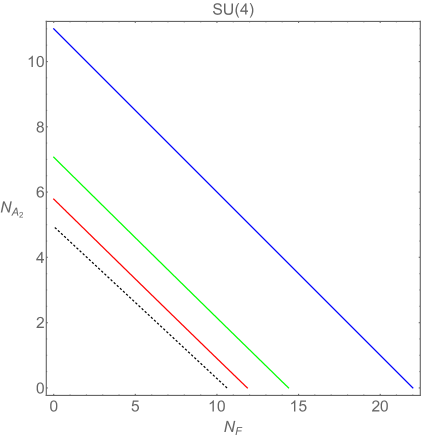
Figure 1: Plot of regions and boundaries in the $(N_{F},N_{A_{2}})$ plane for $G={\rm SU}(4)$. The upper solid line (colored blue) is the solution locus of the equation $b_{1}=0$ and is the upper boundary ${\cal B}_{CW,u}$ of the conformal window. The plot shows the locations of the boundary ${\cal B}_{CW,\ell}$, as calculated in khl from the quadratic $\gamma$CC condition (colored green), and as calculated here from the linear $\gamma$CC condition (colored red). The dashed line is the solution locus of the equation $b_{2}=0$ and is the lower boundary ${\cal B}_{IRZ,\ell}$ of the IRZ region.

We show our results in Fig. 1. The uppermost line (colored blue) is the upper boundary ${\cal B}_{CW,u}={\cal B}_{IRZ,u}$ of the conformal window, given by the condition $b_{1}=0$. The locations of the lower boundary ${\cal B}_{CW,\ell}$ as calculated in khl from the quadratic $\gamma$CC condition (colored green), and as calculated here from the linear $\gamma$CC condition (102), which reduces to (103) (colored red), are shown. Both of these calculations of ${\cal B}_{CW,\ell}$ use the $\kappa^{(F)}_{j}$ and $\kappa^{(A_{2})}_{j}$ calculated to order $j=3$ from the general results in dexm . The dashed line is the solution locus of the equation $b_{2}=0$ and is the lower boundary ${\cal B}_{IRZ,\ell}$ of the IRZ region. For general $N_{c}$ and, in particular, for $N_{c}=4$, the conditions (102) and (103) are nonlinear equations in the variables $N_{F}$ and $N_{A_{2}}$, but the coefficients of the nonlinear terms are small compared to the coefficients of the linear terms and get smaller as the total degree $s+t$ of a term $N_{F}^{s}N_{A_{2}}^{t}$ increases, so that the solution locus is close to being linear in the $(N_{F},N_{A_{2}})$ plane. As is evident in Fig. 1, the use of the linear form of the $\gamma$CC in Eq. (103) yields a boundary ${\cal B}_{CW,\ell}$ that lies to the lower left of the boundary ${\cal B}_{CW,\ell}$ obtained with the use of the quadratic $\gamma$CC condition in the $(N_{F},N_{A_{2}})$ plane. As was discussed in Sect. II.4, this is a consequence of the fact that the quadratic $\gamma$CC condition (34) generates higher-order terms in powers of the scheme-independent expansion variables and leads to different coefficients for lower-order terms. With ${\cal B}_{CW,\ell}$ as determined from (103) and shown in Fig. 1, the (4,4,4) theory is within the conformal window, close to the lower boundary. Along the diagonal $N_{F}=N_{A_{2}}$, the boundary ${\cal B}_{CW,\ell}$ calculated from (103) crosses the point $(N_{F},N_{A_{2}})=(3.88,3.88)$, slightly to the lower left of the point $(N_{F},N_{A_{2}})=(4,4)$. Therefore, with ${\cal B}_{CW,\ell}$ computed via the linear form of the $\gamma$CC condition, (102) or (103), the (4,4,4) theory is in the conformal window. This is in accord with our result that at cubic order in the scheme-independent expansion coefficients, the values of anomalous dimensions that we obtain, namely $\gamma_{\bar{\chi}\chi,IR,\Delta_{A_{2}}^{3}}=0.942$ in Eq. (93) and $\gamma_{\bar{\psi}\psi,IR,\Delta_{F}^{3}}=0.683$ in Eq. (90) in the (4,4,4) theory, are both less than 1. Our comparative analysis showing the difference in the location of the boundary ${\cal B}_{CW,\ell}$ as computed via the quadratic $\gamma$CC condition in khl and as computed via the linear $\gamma$CC condition here (with inputs for the $\kappa^{(A_{2})}_{j}$ and $\kappa^{(F)}_{j}$ calculated up to the same maximal order, $j=3$) provides a quantitative measure of the importance of higher-order terms in the scheme-independent expansions and hence the uncertainty in the determination of the location of ${\cal B}_{CW,\ell}$. This comparison makes it clear that these higher-order corrections are significant.

Since the anomalous dimensions increase as one moves downward within the conformal window toward the lower boundary ${\cal B}_{CW,\ell}$, the linear form of the $\gamma$CC condition implies that for any theory below this lower boundary, at least some fermion $f$ has an anomalous dimension $\gamma_{\bar{f}f,IR}$ that is larger than 1, where here, $\{f\}=\{\psi,\ \chi\}$, i.e., $\{F,A_{2}\}$. A peculiar feature of the quadratic form of the $\gamma$CC condition is that if one uses it to determine ${\cal B}_{CW,\ell}$ with input coefficients $\kappa^{(f)}_{j}$ calculated to the same maximal order as with the linear $\gamma$CC condition, then this boundary ${\cal B}_{CW,\ell}$ from the quadratic $\gamma$CC condition has the property that there are theories that lie outside the conformal window but in which all fermions $f$ have anomalous dimensions $\gamma_{\bar{f}f,IR}$ that are less than 1. This situation occurs here; our direct calculation of $\gamma_{\bar{\psi}\psi,IR}$ and $\gamma_{\bar{\chi}\chi,IR}$ in the (4,4,4) theory, with input values for the $\kappa^{(F)}_{j}$ and $\kappa^{(A_{2})}_{j}$ computed to the $j=3$ order, yields values for $\gamma_{\bar{\chi}\chi,IR,\Delta_{A_{2}}^{3}}$ and $\gamma_{\bar{\psi}\psi,IR,\Delta_{F}^{3}}$ that are both less than 1, but the point $(N_{F},N_{A_{2}})=(4,4)$ lies outside the conformal window, as calculated in khl via the quadratic $\gamma$CC condition with the same inputs for $\kappa^{(F)}_{j}$ and $\kappa^{(A_{2})}_{j}$ computed up to order $j=3$.

To investigate the behavior of $\gamma_{\bar{\psi}\psi,IR,\Delta_{F}^{p}}$ and $\gamma_{\bar{\chi}\chi,IR,\Delta_{F}^{p}}$ for $p=1,2,3$ further in this SU(4) theory, we calculate how they vary as functions of $N_{F}$ and $N_{A_{2}}$, in particular, when one sets $N_{F}=4$ and varies $N_{A_{2}}$ or one sets $N_{A_{2}}=4$ and varies $N_{F}$. These intervals are, respectively, a vertical and a horizontal line segment in the $(N_{F},N_{A_{2}})$ plane, which both pass through the point of primary interest, $(N_{F},N_{A_{2}})=(4,4)$. Our results are presented in Figs. 2-5. As one can see from Figs. 4 and 5, for $N_{F}=4$, this yields the value $N_{A_{2}}=3.8$ as being on ${\cal B}_{CW,\ell}$ calculated from the linear $\gamma$CC condition (103), and for $N_{A_{2}}=4$, it yields the value $N_{F}=3.6$ as being on this boundary. These calculations thus serve as a check on our calculation of the boundary ${\cal B}_{CW,\ell}$ from the linear $\gamma$CC condition (103), since one can verify that this boundary does pass through the points $(N_{F},A_{A_{2}})=(4.0,3.8)$ and (3.6,4.0).

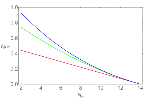
Figure 2: Plot of $\gamma_{\bar{\psi}\psi,IR,\Delta_{F}^{p}}$ calculated to order $p=1,2,3$ for $G={\rm SU}(4)$, and $N_{A_{2}}=4$, as a function of $N_{F}\in I_{IRZ}$. From bottom to top, the curves refer to $\gamma_{\bar{\psi}\psi,IR,\Delta_{F}}$ (red), $\gamma_{\bar{\psi}\psi,IR,\Delta_{F}^{2}}$ (green), and $\gamma_{\bar{\psi}\psi,IR,\Delta_{F}^{3}}$ (blue). The vertical axis is simply labelled as $\gamma_{\bar{\psi}\psi}$ for short.

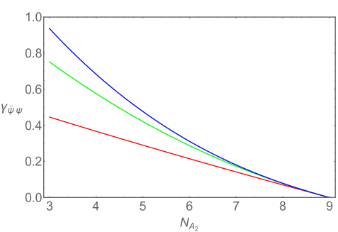
Figure 3: Plot of $\gamma_{\bar{\psi}\psi,IR,\Delta_{F}^{p}}$ calculated to order $p=1,2,3$ for $G={\rm SU}(4)$, and $N_{F}=4$, as a function of $N_{A_{2}}\in I_{IRZ}$. From bottom to top, the curves refer to $\gamma_{\bar{\psi}\psi,IR,\Delta_{F}}$ (red), $\gamma_{\bar{\psi}\psi,IR,\Delta_{F}^{2}}$ (green), and $\gamma_{\bar{\psi}\psi,IR,\Delta_{F}^{3}}$ (blue).

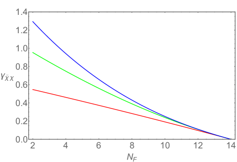
Figure 4: Plot of $\gamma_{\bar{\chi}\chi,IR,\Delta_{A_{2}}^{p}}$, calculated to order $p=1,2,3$ for $G={\rm SU}(4)$, and $N_{A_{2}}=4$, as a function of $N_{F}\in I_{IRZ}$. From bottom to top, the curves refer to $\gamma_{\bar{\chi}\chi,IR,\Delta_{A_{2}}}$ (red), $\gamma_{\bar{\chi}\chi,IR,\Delta_{A_{2}}^{2}}$ (green), and $\gamma_{\bar{\chi}\chi,IR,\Delta_{A_{2}}^{3}}$ (blue). The vertical axis is simply labelled as $\gamma_{\bar{\chi}\chi}$ for short.

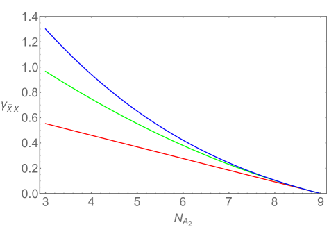
Figure 5: Plot of $\gamma_{\bar{\chi}\chi,IR,\Delta_{A_{2}}^{p}}$, calculated to order $p=1,2,3$ for $G={\rm SU}(4)$, and $N_{F}=4$, as a function of $N_{F}\in I_{IRZ}$. From bottom to top, the curves refer to $\gamma_{\bar{\chi}\chi,IR,\Delta_{A_{2}}}$ (red),$\gamma_{\bar{\chi}\chi,IR,\Delta_{A_{2}}^{2}}$ (green), and $\gamma_{\bar{\chi}\chi,IR,\Delta_{A_{2}}^{3}}$ (blue).

One of the interesting features of this SU(4) theory is that the gauge-singlet particle spectrum contains composite fermion(s), $\{f_{s}\}$. The lattice simulations in fx444 yield anomalous dimensions for several composite-fermion operators, which are found to be $\mathrel{\raisebox{-2.58334pt}{$\stackrel{{\scriptstyle\textstyle<}}{{\sim}}$}}0.5$, smaller than desired for models of a partially composite top quark. Comparison is made with one-loop perturbative calculations of the anomalous dimensions for these gauge-singlet composite fermion operators. In future work, it could be useful to carry out higher-order scheme-independent perturbative calculations of the anomalous dimensions for these composite-fermion operators. This is beyond the scope of our present work, since the requisite higher-order coefficients $c^{(f_{s})}_{\ell}$ in the conventional series expansions (14) have not, to our knowledge, been calculated.

V Conclusions

In this paper we have used our general results in dexm to calculate scheme-independent expansions for anomalous dimensions $\gamma_{\bar{\psi}\psi,IR}$ and $\gamma_{\bar{\chi}\chi,IR}$ of the fermion bilinear operators $\bar{\psi}\psi$ and $\bar{\chi}\chi$ at an infrared fixed point in an asymptotically free SU($N_{c}$) gauge theory with massless fermion content consisting of $N_{F}$ fermions $\psi^{a}_{i}$ in the fundamental representation and $N_{A_{2}}$ fermions $\chi^{ab}_{j}$ in the antisymmetric rank-2 tensor representation. These calculations were performed to the highest order, namely cubic order in the respective expansion variables $\Delta_{F}$ and $\Delta_{A_{2}}$, for which the necessary inputs are available. We have taken the special case $N_{c}=4$ and compared the results with values of these anomalous dimensions in an SU(4) theory with $N_{F}=4$ and $N_{A_{2}}=4$ from a lattice simulation in fx444 . We find agreement with these measured values at the cubic order to which we have performed the perturbative calculations, and we have given estimates of higher-order corrections to our results. More generally, we have studied the dependence of $\gamma_{\bar{\psi}\psi,IR}$ and $\gamma_{\bar{\chi}\chi,IR}$ as functions of $N_{F}$ and $N_{A_{2}}$ in the SU(4) theory and have compared different ways of calculating the lower boundary of the conformal window.

Appendix A Group Invariants

In this appendix we identify our notation for various group invariants. Let $T^{a}_{R}$ denote the generators of the Lie algebra of a group $G$ in the representation $R$, where $a$ is a group index, and let $d_{R}$ denote the dimension of $R$. The Casimir invariants $C_{2}(R)$ and $T_{R}$ are defined as follows: $T^{a}_{R}T^{a}_{R}=C_{2}(R)I$, where here $I$ is the $d_{R}\times d_{R}$ identity matrix, and ${\rm Tr}_{R}(T^{a}_{R}T^{b}_{R})=T(R)\delta^{ab}$. For a fermion $f$ transforming according to a representation $R$, we often use the equivalent compact notation $T_{f}\equiv T(R)$ and $C_{f}\equiv C_{2}(R)$. We also use the notation $C_{A}\equiv C_{2}(A)\equiv C_{2}(G)$. Thus, e.g., for the $F$ and $A_{2}$ representations of SU($N_{c}$), $T(F)=1/2$, $C_{2}(F)=(N_{c}^{2}-1)/(2N_{c})$, $T(A_{2})=(N_{c}-2)/2$, and $C_{2}(A_{2})=(N_{c}-2)(N_{c}+1)/N_{c}$.

The coefficients $\kappa^{(f)}_{j}$ with $j\geq 3$ also involve higher-order group invariants. In general, for a given representation $R$ of $G$,

$$d^{abcd}_{R} = \frac{1}{3!}{\rm Tr}_{R}\Big{[}T^{a}(T^{b}T^{c}T^{d}+T^{b}T^{d}T^{c}+T^{c}T^{b}T^{d}$$ (104)

$$+ T^{c}T^{d}T^{b}+T^{d}T^{b}T^{c}+T^{d}T^{c}T^{b})\Big{]}\ .$$ (106)

In dexm we use the notation $d_{R}^{abcd}\equiv d_{f}^{abcd}$ and for $R=Adj$, we write $d_{R}^{abcd}=d_{A}^{abcd}$. The $\kappa^{(f)}_{3}$ coefficients contain dependence upon products of these $d_{R}^{abcd}$ of the form $d_{R}^{abcd}d_{R^{\prime}}^{abcd}\equiv d_{f}^{abcd}d_{f^{\prime}}^{abcd}$, summed over the group indices $a,\ b,\ c,\ d$. For further details on these higher-order group invariants, see rsv and references therein.

References

- (1) D. J. Gross and F. Wilczek, Phys. Rev. Lett. 30, 1343 (1973); H. D. Politzer, Phys. Rev. Lett. 30, 1346 (1973); G. ’t Hooft, unpublished.
- (2) W. E. Caswell, Phys. Rev. Lett. 33, 244 (1974); D. R. T. Jones, Nucl. Phys. B 75, 531 (1974).
- (3) T. Banks and A. Zaks, Nucl. Phys. B 196, 189 (1982).
- (4) See, e.g., J. Polchinski, Nucl. Phys. B 303, 226 (1988); J.-F. Fortin, B. Grinstein and A. Stergiou, JHEP 01 (2013) 184; A. Dymarsky, Z. Komargodski, A. Schwimmer, and S. Theisen, JHEP 10 (2015) 171.
- (5) T. Appelquist et al., Phys. Rev. D 93, 114514 (2016).
- (6) Y. Aoki et al., Phys. Rev. D 96, 014508 (2017);
- (7) T. Appelquist et al., Phys. Rev. D 99, 014509 (2019); T. Appelquist, J. Ingoldby, and M. Piai, Phys. Rev. D 101 (2020) 075025.
- (8) T. A. Ryttov and R. Shrock, Phys. Rev. D 98, 096003 (2018).
- (9) Taking the fermions to be massless does not incur any loss of generality because a fermion with a nonzero mass would be integrated out of the low-energy effective field theory at Euclidean momentum scales , and hence would be irrelevant to the properties of the theory at the IRFP of interest here.
- (10) S. Girmohanta, T. A. Ryttov, and R. Shrock, Phys. Rev. D 99, 116022 (2019).
- (11) A. Hasenfratz, E. T. Neil, Y. Shamir, B. Svetitsky, and O. Witzel, Phys. Rev. D 107, 114504 (2023).
- (12) B. S. Kim, D. K. Hong, and J.-W. Lee (KHL), Phys. Rev. D 101, 056008 (2020). For the SU(4) theory, KHL use the symbol to refer to the number of Majorana fermions in the representation, while for all we use the symbol to refer to the number of Dirac fermions in the representation, so .
- (13) V. Ayyar, T. DeGrand, M. Golterman, D. Hackett, W. I. Jay, E. T. Neil, Y. Shamir, and B. Svetitsky, Phys. Rev. D 97, 074505 (2016).
- (14) V. Ayyar, T. DeGrand, D. Hackett, W. I. Jay, E. T. Neil, Y. Shamir, and B. Svetitsky, Phys. Rev. D 97, 114505 (2018); Phys. Rev. D 99, 094502 (2019).
- (15) G. Cossu, L. Del Debbio, M. Panero, and D. Preti, Eur. J. Phys. C 79, 638 (2019).
- (16) E. Eichten and K. Lane, Phys. Lett. B 222, 274 (1989); D. K. Hong, S. D. Hsu, and F. Sannino, Phys. Lett. B 597, 89 (2004); D. D. Dietrich, F. Sannino, and K. Tuominen, Phys. Rev. D 72, 055001 (2005); N. D. Christensen and R. Shrock, Phys. Lett. B 632, 92 (2006); D. D. Dietrich and F. Sannino, Phys. Rev. D 75, 085018 (2007); T. A. Ryttov and F. Sannino, Phys. Rev. D 76, 105004 (2007); Phys. Rev. D 78, 115050 (2008); T. A. Ryttov and R. Shrock, Phys. Rev. D 81, 116003 (2010).
- (17) J. B. Kogut and D. K. Sinclair, Phys. Rev. D 81, 114507 (2010); T. DeGrand, Y. Shamir, and B. Svetitsky, Phys. Rev. D 82, 054503 (2010); Phys. Rev. D 87, 074507 (2013); Z. Fodor, K. Holland, J. Kuti, and D. Nogradi, Phys. Lett. B 718, 657 (2012); Z. Fodor, K. Holland, J. Kuti, S. Mondal, and D. Nogradi, JHEP 09 (2015) 039.
- (18) G. Ferretti and D. Karateev, JHEP 03 (2014) 077.
- (19) T. van Ritbergen, A. N. Schellekens, and J. A. M. Vermaseren, Int. J. Mod. Phys. A 14, 41 (1999).
- (20) One early review is simons ; more recent reviews are given in the Lattice 2021 and Lattice 2022 conferences.
- (21) Simons Workshop on Continuum and Lattice Approaches to the Infrared Behavior of Conformal and Quasiconformal Gauge Theories, Jan. 8-12, 2018, T. A. Ryttov and R. Shrock, organizers; http://scgp.stonybrook.edu/archives/21358.
- (22) G. ’t Hooft, Nucl. Phys. B 61, 455 (1973); W. A. Bardeen et al., Phys. Rev. D 18, 3998 (1978).
- (23) O. V. Tarasov, A. A. Vladimirov, and A. Yu. Zharkov, Phys. Lett. B 93, 429 (1980).
- (24) S. A. Larin and J. A. M. Vermaseren, Phys. Lett. B 303, 334 (1993).
- (25) T. van Ritbergen, J. A. M. Vermaseren, and S. A. Larin, Phys. Lett. B 400, 379 (1997).
- (26) F. Herzog, B. Ruijl, T. Ueda, J. A. M. Vermaseren, and A. Vogt, JHEP 02 (2017) 090.
- (27) P. A. Baikov, K. G. Chetyrkin, and J. H. Kühn, Phys. Rev. Lett. 118, 082002 (2017).
- (28) M. F. Zoller, JHEP 10 (2016) 118.
- (29) K. G. Chetyrkin, Phys. Lett. B 404, 161 (1997).
- (30) J. A. M. Vermaseren, S. A. Larin, and T. van Ritbergen, Phys. Lett. B 405, 327 (1997).
- (31) P. A. Baikov, K. G. Chetyrkin, and J. H. Kühn, JHEP 10 (2014) 076; JHEP 04 (2017) 119.
- (32) K. G. Chetyrkin and M. F. Zoller, JHEP 06 (2017) 074.
- (33) T. A. Ryttov, R. Shrock, Phys. Rev. D 83, 056011 (2011).
- (34) C. Pica, F. Sannino, Phys. Rev. D 83, 035013 (2011).
- (35) R. Shrock, Phys. Rev. D 87, 105005 (2013); Phys. Rev. D 87, 116007 (2013).
- (36) T. A. Ryttov and R. Shrock, Phys. Rev. D 94, 105015 (2016).
- (37) T. A. Ryttov and R. Shrock, Phys. Rev. D 86, 065032 (2012); Phys. Rev. D 86, 085005 (2012).
- (38) R. Shrock, Phys. Rev. D 88, 036003 (2013); Phys. Rev. D 90, 045011 (2014).
- (39) T. A. Ryttov, Phys. Rev. Phys. Rev. D 89, 016013 (2014); Phys. Rev. D 89, 056001 (2014); Phys. Rev. D 90, 056007 (2014).
- (40) G. Choi and R. Shrock, Phys. Rev. D 90, 125029 (2014); Phys. Rev. D 94, 065038 (2016).
- (41) J. A. Gracey and R. M. Simms, Phys. Rev. D 91, 085037 (2015).
- (42) J.A. Gracey, R. H. Mason, T. A. Ryttov, and R. M. Simms, arXiv:2306.09056.
- (43) W. Celmaster and R. J. Gonsalves, Phys. Rev. D 20, 1420 (1979); P. M. Stevenson, Phys. Rev.D 23, 2916 (1981); S. J. Brodsky, G. P. Lepage, and P. B. Mackenzie, Phys. Rev. D 28, 228 (1983); S. J. Brodsky, M. Mojaza, and X.-G. Wu, Phys. Rev D 89, 014027 (2014); X.-G. Wu, J.-M. Shen, B.-L. Du, X.-D. Huang, S.-Q. Wang, and S. J. Brodsky, Prog. Part. Nucl. Phys. 108, 103706 (2019) and references therein.
- (44) G. ’t Hooft, in The Whys of Subnuclear Physics, Proc. 1977 Erice Summer School, ed. A. Zichichi (Plenum, New York, 1979), p. 943.
- (45) G. Grunberg, Phys. Rev. D 46, 2228 (1992); E. Gardi and M. Karliner, Nucl. Phys. B 529, 383 (1998); E. Gardi and G. Grunberg, JHEP 03, 024 (1999).
- (46) T. A. Ryttov, Phys. Rev. Lett. 117, 071601 (2016).
- (47) T. A. Ryttov and R. Shrock, Phys. Rev. D 94, 105014 (2016).
- (48) T. A. Ryttov and R. Shrock, Phys. Rev. D 94, 125005 (2016).
- (49) T. A. Ryttov and R. Shrock, Phys. Rev. D 95, 085012 (2017) Phys. Rev. D 95, 105004 (2017).
- (50) T. A. Ryttov and R. Shrock, Phys. Rev. D 96, 105018 (2017).
- (51) T. A. Ryttov and R. Shrock, Phys. Rev. D 96, 105015 (2017);
- (52) T. A. Ryttov and R. Shrock, Phys. Rev. D 97, 025004 (2018).
- (53) T. A. Ryttov and R. Shrock, Phys. Rev. D 101, 076018 (2020).
- (54) J. A. Gracey, T. A. Ryttov, and R. Shrock, Phys. Rev. D 97, 116018 (2018).
- (55) V. A. Novikov, M. A. Shifman, A. I. Vainshtein, and V. I. Zakharov, Phys. Lett. B 166, 329 (1986).
- (56) N. Seiberg, Nucl. Phys. B 435, 129 (1995; K. A. Intriligator and N. Seiberg, Nucl. Phys. B. Proc. Suppl. 45, 1 (1996).
- (57) T. Appelquist, K. D. Lane and U. Mahanta, Phys. Rev. Lett. 61, 1553 (1988).
- (58) A. G. Cohen and H. Georgi, Nucl. Phys. B 314, 7 (1989).
- (59) D. B. Kaplan, J.-W. Lee, D. T. Son, and M. A. Stephanov, Phys. Rev. D 80, 125005 (2009).
- (60) R. Zwicky, arXiv:2306.06752.
- (61) J.-W. Lee, Phys. Rev. D 103, 076006 (2021).
- (62) Some of the relevant papers before the Higgs discovery include W. A. Bardeen, C. N. Leung and S. T. Love, Phys. Rev. Lett. 56, 1230 (1986); K. Yamawaki, M. Bando and K. Matumoto, Phys. Rev. Lett. 56, 1335 (1986); B. Holdom, Phys. Lett. B 150, 301 (1985); B. Holdom and J. Terning, Phys. Lett. B 187, 357 (1987); T. Appelquist, D. Karabali, and L. C. R. Wijewardhana, Phys. Rev. Lett. 57, 957 (1986); V. A. Miransky, M. Tanabashi, and K. Yamawaki, Phys. Lett. B 221, 177 (1989); T. Appelquist, J. Terning, and L. C. R. Wijewardhana, Phys. Rev. Lett. 77, 1214 (1996); W. D. Goldberger, B. Grinstein and W. Skiba, Phys. Rev. Lett. 100, 111802 (2008); T. Appelquist and Y. Bai, Phys. Rev. D 82, 071701 (2010); L. Vecchi, Phys. Rev. D 82, 076009 (2010); M. Hashimoto and K. Yamawaki, Phys. Rev. D 83, 015008 (2011).
- (63) ATLAS Collab., Nature 607, 52 (2022); CMS Collab., Nature 607, 60 (2022).
- (64) See, e.g., reviews by M. Carena, C. Grosjean, and M. Kado, and by K. M. Black, R. S. Chivukula, and M. Narain, in Particle Data Group, Review of Particle Properties, at http://pdg.lbl.gov.
- (65) T. Appelquist and R. Shrock, Phys. Lett. B 548, 204 (2002); Phys. Rev. Lett. 90, 201801 (2003); T. Appelquist, M. Piai, and R. Shrock, Phys. Rev. D 69 015002 (2004); N. D. Christensen and R. Shrock, Phys. Rev. Lett. 94, 241801 (2004).
- (66) G. Mack, Commun. Math. Phys. 55, 1 (1977).
- (67) B. Grinstein, K. Intriligator, and I. Rothstein, Phys. Lett. B 662, 367 (2008)
- (68) Y. Nakayama, Phys. Rept. 569, 1 (2015).
- (69) G. A. Baker and P. Graves-Morris, Padé Approximants, Encyclopedia of Math. v. 13 (Addison-Wesley, Reading, 1981).
- (70) Our notation follows I-H. Lee and R. E. Shrock, Phys. Rev. B 36, 3712 (1987); J. Phys. A 21, 3139 (1988); V. Matveev and R. Shrock, J. Phys. A 28, 1557 (1995).