The Importance of Heat Flux in Quasi-Parallel Collisionless Shocks

Abstract

Collisionless plasma shocks are a common feature of many space and astrophysical systems and are sources of high-energy particles and non-thermal emission, channeling as much as 20% of the shock’s energy into non-thermal particles. The generation and acceleration of these non-thermal particles have been extensively studied, however, how these particles feed back on the shock hydrodynamics has not been fully treated. This work presents the results of self-consistent hybrid particle-in-cell simulations that show the effect of self-generated non-thermal particle populations on the nature of collisionless, quasi-parallel shocks. They contribute to a significant heat flux density upstream of the shock. Non-thermal particles downstream of the shock leak into the upstream region, taking energy away from the shock. This increases the compression ratio, slows the shock down, and flattens the non-thermal population’s spectral index for lower Mach number shocks. We incorporate this into a revised theory for the Rankine-Hugoniot jump conditions that include this effect and it shows excellent agreement with simulations. The results have the potential to explain discrepancies between predictions and observations in a wide range of systems, such as inaccuracies of predictions of arrival times of coronal mass ejections and the conflicting radio and x-ray observations of intracluster shocks. These effects will likely need to be included in fluid modeling to accurately predict shock evolution.

1 Introduction

Shock waves are ubiquitous plasma phenomena occurring in many heliospheric and astrophysical contexts, including systems such as Earth’s bow shock, interplanetary coronal mass ejections, the heliospheric termination shock, binary stellar wind interactions, supernovae, and Galaxy cluster mergers (Burgess & Scholer, 2015; Lee et al., 2012; Ellison et al., 2007; Ryu et al., 2003; Kang et al., 2012). There are two characteristic features that all of these systems share:

1. They occur in environments where the collisional mean free path is much larger than the other fundamental plasma length scales, e.g., the proton gyro-radius.

2. They are sources of energetic particles and non-thermal emission.

These characteristics of astrophysical plasma shocks are potentially important to their evolution which can result in a significant deviation of their behaviour from collisional, fluid shocks.

Previous simulations and theoretical works have connected these two features showing that non-thermal particles are generated and accelerated by collisionless shocks (e.g., Bell (1978, 2004); Caprioli & Spitkovsky (2014a)). The non-thermal particles are initially energized by the reformation of the shock until reaching an energy $E$ for which the particle gyro-radius is sufficiently large relative to the width of the shock front ($E/E_{sh}\gtrapprox 10$, with $E_{sh}=m_{i}u_{1}^{2}/2$ being the kinetic energy of the upstream bulk flow in the shock frame, where $m_{i}$ is the ion mass and $u_{1}$ is the upstream velocity in the shock frame) (Caprioli et al., 2015). Above this energy, non-thermal particles can freely move upstream and downstream of the shock and continue to be energized by successive collisionless scatterings between these two regions, in a process referred to as diffusive shock acceleration, or DSA (Krymskii, 1977; Bell, 1978; Blandford & Ostriker, 1978).

The non-thermal population, while few in number, can account for order 10% of the shock’s ram energy density ($n_{1}E_{sh}$, where $n_{1}$ is ion number density in the upstream region) (Völk et al., 2005; Parizot et al., 2006; Caprioli et al., 2008; Morlino & Caprioli, 2012; Slane et al., 2014; Johlander et al., 2021). The relatively large fraction of energy channeled into non-thermal particles, coupled with the collisionless nature of the shock implies that the ion distribution functions are non-Maxwellian, which violates a core assumption of the fluid modeling of shocks. This means that the standard hydrodynamic shock treatment, i.e., the Rankine–Hugoniot jump conditions, is an incomplete description of the properties of the shock (O’C. Drury & Völk, 1981; Morlino & Caprioli, 2012; Bret, 2020; Haggerty et al., 2022). Previous studies have worked towards developing more a complete description and predicting the self-generated non-thermal population’s effect on the shock dynamics; these shocks are referred to as cosmic ray (CR) modified shocks (O’C. Drury, 1983; Blandford & Eichler, 1987; Jones & Ellison, 1991; Malkov & O’C. Drury, 2001; Caprioli et al., 2009b, a, 2010). Additionally, more recent works have begun including the effects of non-thermal particles on the physics of fluid shock models which can reproduce some features predicted by CR-modified shock theory, with results that strongly depend on the non-thermal particle energy (Pfrommer et al., 2017). However, this quantity must be set a posteriori.

In this work, we demonstrate the effect of a self-generated, non-thermal population on the nature of the shock, from first principles using self-consistent hybrid particle-in-cell simulations. We show that the non-thermal particles downstream of the shock leak into the upstream region, taking energy away from the shock, increasing its compressibility, and slowing the shock down. Upstream of the shock, these escaping non-thermal particles create a large heat flux density, which has been suggested to be important in previous works (Alves & Fiuza, 2022). However, this large heat flux is counterbalanced by an equal and opposite enthalpy flux in the upstream region, a condition that is required for the stationary of the shock (i.e., for it to be unchanging in time). This process causes an increase in the compression ratio and a flattening of the self-generated non-thermal population’s spectral index for lower Mach number shocks. This result implies that collisionless shocks will travel on the order of $\approx 10\%$ slower than standard hydrodynamic predictions, for systems with efficient non-thermal particle acceleration, which is a seemingly universal feature of quasi-parallel shocks. We present a simple revised theory for the Rankine-Hugoniot jump conditions including this effect which yields results consistent with simulations. Finally, we argue that this effect can account for discrepancies between predictions and observations in shocks ranging from arrival times of coronal mass ejections to non-thermal spectra of Galaxy cluster mergers, attesting to the potential universality of this result. The former has far-reaching implications for space weather prediction and readiness.

2 Non-Thermal Particles in Quasi-Parallel Shocks

In this section we show that the pressure from self-generated, non-thermal particles should be large enough to considerably reduce collisionless shock compression ratios, which is at odds with both observations and simulations, motivating a reevaluation of the jump conditions. Non-thermal particles are efficiently accelerated by quasi-parallel shocks, i.e., shocks where the direction of propagation is quasi-parallel to the magnetic field in the upstream plasma, quantified by the angle $\theta_{B_{n}}=\cos^{-1}(|B_{x}|/|\vec{B}|)\lessapprox 45^{\circ}$, where $\vec{B}$ is the magnetic field vector and the $x$-direction is normal to the shock propagation (e.g., Morlino & Caprioli (2012); Caprioli & Spitkovsky (2014a); Johlander et al. (2021). In these systems, non-thermal particles with $E\gtrsim 10E_{sh}$ are free to travel upstream and downstream of the shock since their gyro-radius is larger than the shock width. This leakage of the non-thermal population exerts pressure on the inflowing upstream plasma, weakening the shock in two ways (Ellison et al., 2007; Caprioli et al., 2008; Haggerty & Caprioli, 2020; Caprioli et al., 2020): reducing the inflow speed and increasing the upstream temperature, which combine to reduce the sonic or magnetosonic Mach number (Burgess & Scholer, 2015).

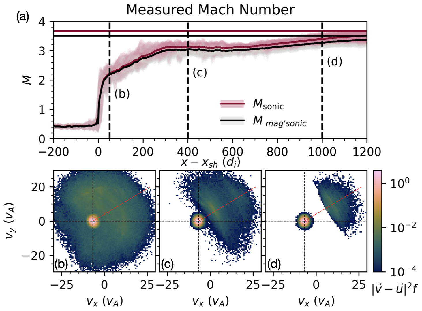
Figure 1: (a) The locally defined sonic and magnetosonic Mach numbers measured in the shock simulation as a function of distance to the shock front, with the horizontal lines showing the far-upstream value. The values are averaged over the $y$ direction with the darker lines corresponding to values averaged in time over $100\Omega_{ci}^{-1}$, and the lighter lines show the individual slices that make up the time average. (b) - (d) Ion distribution functions at the locations shown by the dashed lines in (a), scaled by $|\vec{v}-\vec{u}|^{2}$. The distribution functions are plotted in the $v_{x}$, $v_{y}$ plane and integrated over the $v_{z}$ direction.

Of the two effects, the increased upstream temperature is more significant because of the non-thermal particles high energy and has a $v^{2}$ dependence in the second moment of the distribution. Simulations and observations have consistently shown that on the order of 10% of the shock’s available energy density is channeled into non-thermal particle energy density (Caprioli & Spitkovsky, 2014a, b; Haggerty & Caprioli, 2020; Morlino & Caprioli, 2012; Ackermann et al., 2013), $\xi\equiv P_{cr}/\rho_{1}u_{1}^{2}\approx 0.1$ where $P_{cr}$ is the pressure in the non-thermal particles and $\rho_{1}$ is the upstream mass density. This implies that if we were to naively define the effeictive sonic Mach number $M_{\rm eff}$ including the non-thermal particles, the effective Mach number for quasi-parallel shocks would always be reduced, according to $M_{\rm eff}=u_{1}/\sqrt{\Gamma(P_{1}+P_{cr}/\rho_{1}}\sim 2.5$, where $\Gamma=5/3$ is the adiabatic index, assuming that the most of the non-thermal energy is carried by non-relativistic particles. However, we will show that while this non-thermal population is present near the shock, the effective mach number defined in this way, i.e., based on the second moment of the distribution function, is inconsistent with the shock hydrodynamics.

This reduction in the effective Mach number is evident in simulations as shown in Fig. 1, which shows results from a quasi-parallel shock simulation performed with the self-consistent, hybrid particle-in-cell dHybridR code (see Appendix A for details on the code and the simulation used in this work). The red and black lines in panel (a) show the effective sonic ($M_{sonic}$) and fast magneto-sonic )($M_{mag^{\prime}sonic}$ Mach numbers (defined in Appendix A, (Wilson III et al., 2019)), respectively, as a function of normal distance to the shock ($x-x_{sh}$) along a cut through the simulation. The darker lines correspond to the value averaged over 200 consecutive cuts in time spaced out over 100 $\Omega_{ci}^{-1}$, with the lighter lines showing each of the individual cuts that make up the average. The upstream plasma far away from the shock has sonic, magnetosonic, and Alfvénic Mach numbers of $3.51,\ 3.67,$ and $6.7$, respectively, illustrated as the straight horizontal lines and corresponding to an upstream $\beta_{i}=\beta_{e}=2$. Note that since the shock simulations are performed in the downstream frame, the actual Mach number, as defined in the shock frame, can only be determined after the shock has formed and its speed can be determined empirically. Far upstream, the effective Mach number $M_{\rm eff}\approx M_{s}$, however closer to the shock $M_{\rm eff}$ drops significantly, reaching a value of nearly $M_{\rm eff}\approx 2.3$. This change is attributed to the extensive non-thermal population, which can be seen in the reduced distribution functions plotted in Fig. 1(b)-(d), where $f(v_{x},v_{y})$ has been integrated over $v_{z}$ and is weighted by the difference in velocity to the upstream bulk flow squared $|\vec{v}-\vec{u}|^{2}$. Each of the sub-panels corresponds to the different locations as indicated by the vertical dashed lines in panel (a). The distribution functions are cumulative over time and the averaging window is a $2\times 2d_{i}^{2}$ box at $y=10d_{i}$ and different locations in $x$. The red dashed line indicates the direction of the upstream magnetic field. Close to the shock front, there is a significant fraction of non-thermal particles, i.e., the ion precursor region, which are attenuated with distances farther from the shock, where only a limited, field-aligned fraction can reach.

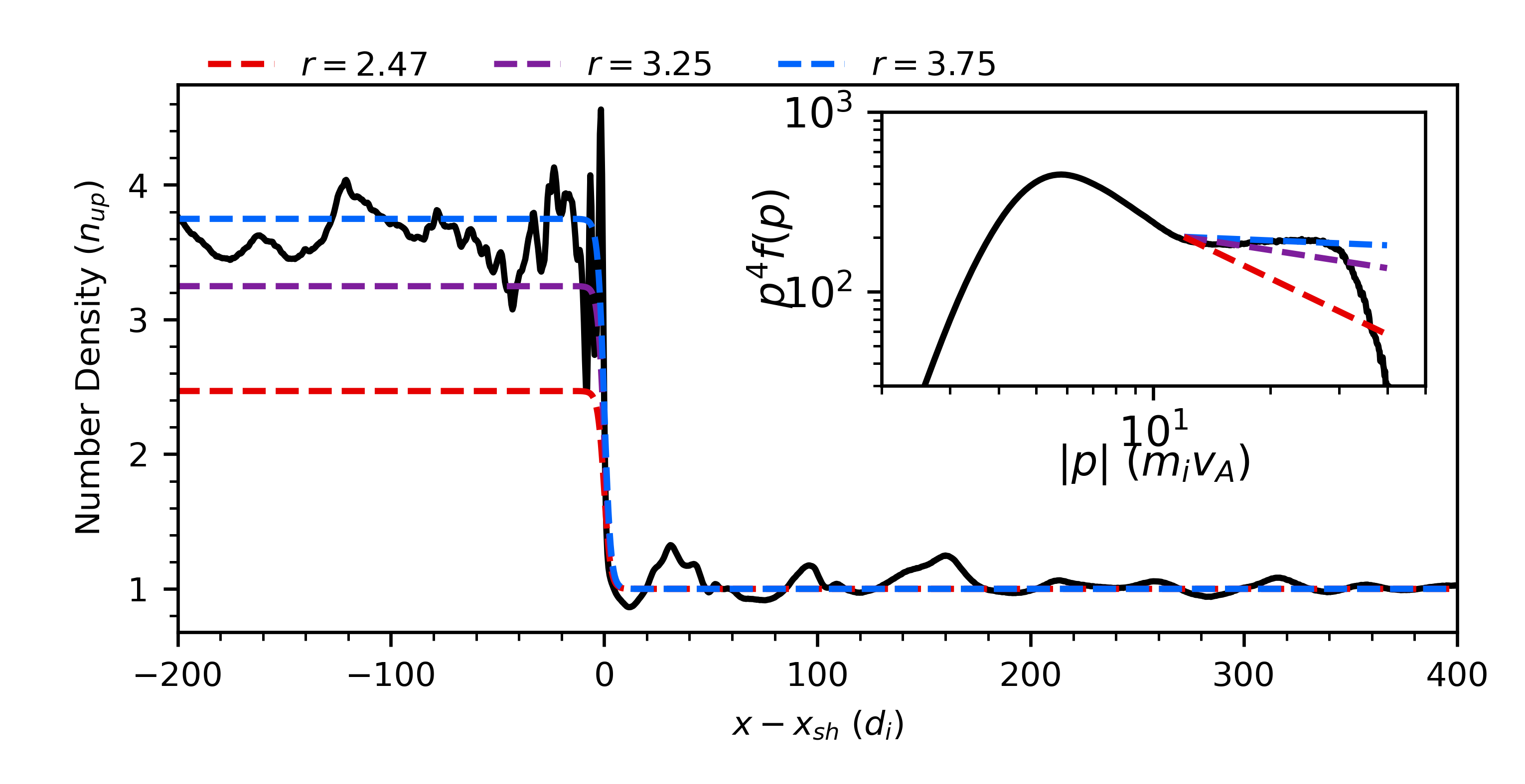
Figure 2: The ion number density averaged over the $y$ direction and plotted as a function of normal distance from the shock front at time $t=160\Omega_{ci}^{-1}$. The dashed lines correspond to predictions for the compression ratio based on different Mach numbers: the red line is from a Mach number based on the temperature just upstream of the shock (location (b) in Fig. 1(a), $M=2.55$, using the standard formula $r=(\Gamma+1)/(\Gamma-1+2/M^{2})$), the purple line shows predictions for the shock compression ratio based on the Mach number far upstream of the shock ($M=3.67$), and the blue dashed line shows the prediction derived in this work including the heat flux and enthalpy flux of the self-generated, non-thermal particles (Eq. C13). The inset shows the average downstream distribution function (multiplied by $p^{4}$) as a function of momentum. The predicted non-thermal power law indices are shown by the dashed lines based on standard DSA theory from the corresponding compression ratios.

Applying the overly simplified definition for the effective Mach number $50d_{i}$ upstream of the shock front to the standard Rankine-Hugoniot jump conditions predicts a weak shock with a compression ratio of $\sim 2.5$ for not only this shock but for any shock with efficient non-thermal acceleration (i.e., $\xi\sim 0.1$). However, this prediction is at odds with observations and simulations of collisionless shocks, and even for the simulation presented in this manuscript. Fig. 2 shows a cut of the ion number density as a function of distance from the shock front, from this the compression ratio of the shock can be inferred as the asymptotic upstream density is 1. The red dashed line shows the prediction based on $M_{\rm eff}$, while the purple dashed line shows the prediction based on $M_{s}$, i.e., the sonic Mach number without the non-thermal contribution. The measured compression ratio is larger than either of these predictions. Moreover, the spectral index of the non-thermal, power law distribution is consistent with this enhanced compression, i.e., the power-law distribution following $f\sim p^{-q}$ where $q$ is determined solely by the compression ratio $q=3r/(r-1)$ (Krymskii, 1977; Bell, 1978). This is shown in the inset figure, where the dashed lines correspond to standard DSA predictions The resolution to this apparent discrepancy comes from the closure of the fluid equations and the incompleteness of standard Rankine-Hugoniot jump conditions for describing a collisionless plasma.

3 Heat Flux in the Jump Conditions

The shock jump conditions are derived within the fluid approximation, which implicitly assumes the shape of the particle distribution functions $f$ must be drifting Maxwellian distributions. Because of this assumption, the jump condition describing the energy flux density on either side of the shock omits the heat flux density, a third-order moment of the distribution function, defined for an arbitrary distribution as $Q_{j}=(m/2)\int(v_{j}-u_{j})|\vec{v}-\vec{u}|^{2}fd^{3}v$ for a species with mass $m$. However, this assumption is not applicable for the upstream region of a collisionless shock when non-thermal particles are present, as is demonstrated by the distribution functions shown in Fig. 1(b)-(d). Close to the shock front, the significant presence of energetic, non-thermal particles suggests that heat flux density is comparable to the flux of both the bulk flow energy density and thermal energy density, or more precisely the enthalpy flux density (see Appendix B for details).

The importance of the heat flux on the jump conditions is quantified directly in Eqs. 1-3 and in Fig. 3, which shows the various quantities determined from the simulations including those that make up the jump conditions and the heat flux. Each quantity is determined in the shock rest frame (as measured in the simulation) and the figure employs the same time averaging used in Fig. 1. Fig. 3 shows the individual components and total of the following jump conditions :

$$\left[\rho u_{x}\right]=0,$$ (1)

$$\left[\rho u_{x}^{2}+P_{x,x}\right]=0,$$ (2)

$$\left[\frac{1}{2}u_{x}\left(\rho u^{2}+P_{j,j}\right)+u_{j}P_{x,j}+Q_{x}\right]=0,$$ (3)

with Eqs. 1, 2 & 3 corresponding to the first, second and third panels of Fig. 3, respectively, and where the Einstein summation convention is used for repeated dummy indices. The square brackets correspond to the difference between any point in the upstream and downstream regions where the assumption of stationary remains valid. In Eqs. 1 – 3, $P_{j,k}$ is the $j,k$th component of the total pressure tensor (ions, electrons and non-thermals) and $Q_{x}$ is the heat flux density normal to the shock. The contribution of the magnetic field is ignored in the jump conditions because the amplified fields are relatively small for quasi-parallel, lower Mach number shocks (as shown in Fig. 3), however their inclusion into the jump conditions is straightforward. Note that we have yet to make any assumptions about the nature of the distribution function; all of these terms represent generic moments of the distribution function, however in the isotropic limit the pressure tensor terms can be rewritten in the familiar form of $\Gamma P/(\Gamma-1)$.

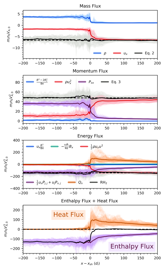
Figure 3: Time-averaged Rankine-Hugoniot jump conditions. 1D cuts normal to the shock and centered around the shock front time-averaged as discussed in Fig. 1. The black lines in each of the panels correspond the sum of the fluxes in Eq. 1, 2, and 3. The colored lines correspond to the different terms in each of the equations. The bottom panel shows the sum (black line) of the heat flux density (orange) and the non-thermal enthalpy flux density (purple). The two almost perfectly counterbalance each other in the upstream region, showing that the upstream, non-thermal particles do not contribute to the jump conditions.

The momentum and energy flux in Fig. 3 confirm what was evident from the upstream distribution functions of Fig. 1; the non-thermal particles have a zeroth order contribution to the upstream terms in the jump conditions, in the pressure flux (purple line, second panel), enthalpy density flux (purple line, third panel) and heat flux density (orange line, third panel). While each of these terms are comparable to either the momentum or bulk energy density flux in the upstream flow, the energy flux panel reveals a critical relationship between these terms. In the upstream region, the heat flux density is nearly equal in magnitude and opposite in sign to the enthalpy flux that has been enhanced by the non-thermal particles. Physically this corresponds to the non-thermal particles traveling away from the shock, carrying energy with them. In the upstream region, the sum of all of the components (black line) is almost exactly equal to the ram energy density flux (red line), which confirms that the heat and enthalpy flux densities negate one another. This cancellation can be interpreted as the balancing of the non-thermal diffusive flux away from the shock with the advection of the non-thermal population towards the shock with the thermal population’s bulk flow. This result suggests that the non-thermal population does not contribute to the upstream energy budget and therefore should not be included in definition of the Mach number. We will show this accounts for the compression ratio exceeding the standard prediction shown in Fig. 2.

4 Including Heat Flux into the shock hydrodynamic predictions

We incorporate the cancellation of the heat and enthalpy fluxes in the upstream region into the jump conditions by splitting the pressure term into the sum of two terms, the thermal (gas) and the non-thermal pressure, $P_{g}$ and $P_{cr}$, respectively. Note that the total mass density and bulk flow are not appreciably altered by the non-thermal particles, as can be seen in Fig. 1 and the first panel of Fig. 3. This substitution will modify the jump conditions in two key ways. First, the pressure in Eq. 2 (the momentum flux equation) is only the thermal pressure $P_{g}$. This is the case because the pressure of the non-thermal population is the same upstream and downstream of the shock, as they are free to pass the shock with impunity. Second, the heat flux density is removed from Eq. 3 along with the non-thermal enthalpy flux density in the upstream region. This leaves a non-thermal contribution to the enthalpy flux density in the downstream side of the equation (see Eq. C8 in Appendix C), which acts as an energy sink. The non-thermal particles contribute to the pressure in the downstream region, but not in the upstream region. Physically, this increases the compressibility of the shock, causing the shock to slow down.

We can explicitly solve for the compression ratio using the modified jump conditions with the inclusion of the normalized non-thermal pressure $\xi$, and the exact solution is derived in Appendix C (Eq. C13). However the prediction can be simplified in the limit of realistic non-thermal efficiencies ($\xi\sim 0.1$):

$$r\approx\frac{(\Gamma+1)M^{2}}{2+(\Gamma-1)M^{2}}+\frac{\Gamma(\Gamma+1)}{\Gamma-1}\xi$$ (4)

The first term in Eq. 4 is the standard RH prediction for an unmodified shock and the second term is positive and linear in $\xi$ which means that the non-thermal population will increase the comparability the of shock (consistent with Fig. 2). As $\xi\rightarrow 0$, Eq. C13 (and Eq. 4) converges to the compression ratio prediction from the standard Rankine-Hugoniot jump conditions. Finally, Eq. 4 can be further simplified in the limit of large $M_{mag^{\prime}sonic}$:

$$r\approx 4(1+\Gamma\xi),.$$ (5)

It should be noted that this accounts for only the hydrodynamic effects from the heat flux, but omits the contribution of the non-thermal postcursor discussed in Haggerty & Caprioli (2020), which will be important for higher Mach number shocks.

In observations and simulations of quasi-parallel collisionless shocks, $\xi$ is consistently found to be on the order of $0.1$ (Völk et al., 2005; Parizot et al., 2006; Caprioli et al., 2008; Caprioli & Spitkovsky, 2014a; Haggerty & Caprioli, 2019; Johlander et al., 2021). Applying this to Eq. 5, we find that the compression ratio of strong quasi-parallel shocks should increase over the standard Rankine-Hugoniot prediction by a factor of $\Gamma/10=1/6\approx 17\%$. Using Eq. 4 and the simulation measured value of $\xi\approx.075$, we find agreement between the measured and predicted compression ratio in the simulation (blue dashed line, Fig. 2).

5 Implications for Space and Astrophysical Shocks

The hydrodynamic modifications outlined in this paper are expected to be a generic feature of any collisionless shock with a non-thermal population (e.g., quasi-parallel configurations), which implies that these results have a considerable impact on disparate systems including solar, heliospheric, and astrophysical. The non-thermal enhancement of the shock compressibility has three immediate implications: First, the compression ratio of quasi-parallel shocks is larger than the standard hydrodynamic prediction, reaching or surpassing the hydrodynamic maximum of 4, even for low Mach number shocks. Second, quasi-parallel shocks travel slower than fluid theory predicts, where the fractional decrease in speed is comparable to the fraction of energy channeled into non-thermal particles (i.e., on the order of 10%, as the speed of the shock in the unshocked frame is given by $u_{s}h\propto 1/(1-1/r)$). Third, the slopes of non-thermal, power law distributions are flatter for a given Mach number, as the slope increases with the compression ratio as predicted by DSA.

The compressional enhancement and associated shock speed reduction have significant implications for numerous astrophysical systems, including the lifetime and evolution of supernova remnants, stellar termination shocks, planetary bow shocks and astrophysical jets. However, perhaps the most important application for this result is for the propagation of interplanetary coronal mass ejections (ICMEs), the accurate modeling of which is crucial for space weather forecasting. Various hydrodynamic and magneto-hydrodynamic (MHD) models for ICMEs consistently underestimate Earth arrival times by approximately 10 hours (e.g., (Dumbović et al., 2018)). Given that ICMEs are efficient sources of solar energetic particles (Reames, 2013; Webb & Howard, 2012; Kamijima et al., 2020), the physics described in this manuscript is expected to be applicable, and to likely account for the order 10% decrease in ICME speeds and an average 10 hour increase in transit time (typically on the order of 100 hours) (Gopalswamy et al., 2001; Dumbović et al., 2018).

Additionally, the flattening of the power law spectrum has far-reaching implications for the acceleration of cosmic rays and high energy emission from shocks. This effect could explain an observational discrepancy in the shocks from galaxy cluster mergers, in which the shock Mach numbers are inferred from x-ray observations, while the spectral index is inferred from radio emission (e.g., van Weeren et al. (2019); Ha et al. (2023)). The observed spectral indices consistently correspond to a larger Mach number than is inferred from the X-ray observations. The effect described in this manuscript explains such measurments and Eq. C13 can be used to bridge these observations. For example, for the Sausage relic (CIZA J$2242.8+5301$), the Mach number is estimated using the radio spectral index of $4.2$, which would correspond to a compression ratio of $3.6$ and a Mach number of $4.6$ (van Weeren et al., 2010), while the value estimated through temperature measurements through X-ray observations is smaller with $M\approx 2.5-3.1$ (Ogrean et al., 2014; Akamatsu et al., 2015). Using Eq. C13 with a Mach number of $2.7$, a compression ratio of $3.6$ would be predicted with a non-thermal/CR efficiency of only $\xi\approx 0.15$, which would completely account for the observational discrepancies.

These are only a few of the potential applications for the results presented in this paper, but there are numerous other potential systems where these results may be significant, including planetary bow shocks, solar/stellar wind termination shocks and supernova remnants. One potential system in which these results could be constrained and potentially applied is Earth’s day-side magnetosphere, which exhibits strong dawn-dusk asymmetries of the shape of Earth’s bow shock(Walsh et al., 2014; Dimmock et al., 2017). One proposed source of this dawn-dusk asymmetry is the corresponding quasi-parallel-to-quasi-perpendicular transition of the shock. The asymmetry has been correlated with the presence of energetic ions (Anagnostopoulos et al., 2005; Johlander et al., 2021), which suggests that this paper’s results may, in-part, account for the observed symmetry breaking. While there has been an estimate of the energy budget of the quasi-perpendicular bow shock (Schwartz et al., 2022), a detailed local accounting of the quasi-parallel bow shock is limited by the available in-situ satellites in operation. Constraining these results, and higher moment, kinetic results from shocks more generally, will likely require a multi-spacecraft mission designed for the plasma environment upstream of Earth’s bow shock such as the Multi-point Assessment of the Kinematics of Shocks (MAKOS) mission (Goodrich et al., 2022).

6 Conclusion

In this manuscript, we demonstrate the importance of self-generated non-thermal particles in shock hydrodynamics and show that it is a ubiquitous feature of collisionless quasi-parallel shocks. We develop updated Rankine-Hugoniot jump conditions to include these inherently kinetic effects including the heat flux density associated with non-thermal particles and show they agree well with simulations. We show that the generation of non-thermal particles increases a shock’s compressibility, decreases the propagation speed, and flattens the associated power-law spectrum. We argue that this should be a generic feature of collisionless shocks with non-thermal particles and find that this effect can likely answer several outstanding issues with heliospheric and astrophysical shocks.

7 Acknowledgements

Simulations were performed on computational resources provided by the University of Chicago Research Computing Center, on TACC’s Stampede2 and Purdue’s ANVIL through ACCESS (formally XSEDE) allocation TG-AST180008. C.C.H. was partially supported by NSF FDSS grant AGS-1936393 as well as NASA grants 80NSSC20K1273 and 80NSSC23K0099; D.C. by NASA grant 80NSSC20K1273 and NSF grants AST-1909778, AST-2009326 and PHY-2010240; P.A.C. by NSF PHY-1804428, DOE DE-SC0020294, NASA 80NSSC19M0146 and 80NSSC22K0323.

Appendix A Simulations and dHybridR

To study the effects of heat flux and non-thermal enthalpy flux on the hydrodynamics of shocks, we perform self-consistent simulations using dHybridR, a relativistic hybrid code with kinetic ions and massless, charge-neutralizing fluid electrons (Haggerty & Caprioli, 2019). dHybridR is the generalization of the non-relativistic code dHybrid (Gargaté et al., 2007), which was widely used for simulating collisionless shocks (Gargaté & Spitkovsky, 2012; Caprioli & Spitkovsky, 2014a, b, c; Caprioli et al., 2015, 2017, 2018; Haggerty et al., 2019; Caprioli & Haggerty, 2019).

All physical quantities are normalized to their far upstream initial values, namely: mass density to $\rho_{0}\equiv m_{i}n_{0}$ (with $m_{i}$ the ion, namely proton, mass), magnetic fields to $B_{0}$, lengths to the ion inertial length $d_{i}=c/\omega_{pi}$ (with $c$ the speed of light and $\omega_{pi}$ the ion plasma frequency), time to the inverse ion cyclotron frequency $\Omega_{ci}^{-1}$, and velocity to the Alfvén speed $V_{A0}=B_{0}/\sqrt{4\pi\rho_{0}}$. The ion plasma beta is chosen to be $\beta_{i}=2$, which corresponds to a thermal gyroradius of $1\,d_{i}$. The system is 2.5D; 2D in real space (in the $x-y$ plane), but with all three components of momentum and electromagnetic fields retained. The electrons are chosen to have an adiabatic equation of state, i.e., the electron pressure is $P_{e}\propto\rho^{5/3}$.

The simulation is initialized with a uniform magnetic field ${\vec{B}_{0}}=B_{0}(\cos(30^{\circ})\hat{x}+\sin(30^{\circ})\hat{y})$ (i.e., $\theta_{B_{n}}=30^{\circ}$) and an inflowing thermal ion population with a bulk flow $\vec{u}_{x}=-5V_{A0}\vec{x}$ in the simulation frame. The simulation is periodic in the $y$ direction, the right boundary is open and continuously injecting thermal particles, and the left boundary is a reflecting wall; after tens of cyclotron times, the ions initially closest to the wall reflect and form a shock that travels in the $+\vec{x}$ direction, with the downstream plasma at rest in the simulation reference frame. Note that the speed of the shock in the downstream (simulation) frame is not the same speed that goes into the determination of the Mach number. The Mach number that enters the stationary jump conditions is measured in the shock frame which is determined empirically from the simulation ($\approx 1.7V_{A}$ in the simulation frame), with the sonic and fast magneto-sonic Mach numbers defined as $M_{\rm sonic}=u_{1}/v_{s,1}$ and $M_{\rm mag^{\prime}sonic}=u_{1}/v_{m,1}$, where

$$v_{s,1} =\sqrt{\frac{\Gamma P_{1}}{\rho_{1}}}$$ (A1)

$$v_{A,1} =\frac{B_{1}}{\sqrt{4\pi\rho_{1}}}$$ (A2)

$$v_{m,1} =\left[\frac{1}{2}\left(v_{A,1}^{2}+v_{s,1}^{2}+\sqrt{(v_{A,1}^{2}+v_{s,1}^{2})^{2}-4v_{A,1}^{2}v_{s,1}^{2}\cos^{2}\theta_{Bn}}\right)\right]^{1/2}$$ (A3)

The simulation domain size is $[L_{x},\,L_{y}]=[2000,25]d_{i}$, wide enough to account for 2D effects and long enough so that the simulation could be run $100$s of $\Omega_{ci}^{-1}$ without energetic particles escaping the domain. The simulation has two grid cells per $d_{i}$, and each grid cell is initialized with 10000 particles per grid. The speed of light is set to be larger than the Alfvén and thermal speeds ($c/V_{A0}=c/v_{thi}=50$), as discussed in Haggerty & Caprioli (2019); the time step is set as $c\Delta t=d_{i}/2$.

Appendix B Energy Jump Conditions Including Heat Flux and Enthalpy Flux

The third jump condition including kinetic contributions (Eq. 3) is derived from the sum of the ion and electron Vlasov equation assuming a constant solution in time:

$$\sum_{s}^{i,e}\left[\frac{\partial}{\partial x}(v_{x}f_{s})+\vec{\nabla}_{v}\cdot\frac{q_{s}}{m_{s}}(\vec{E}+\frac{\vec{v}}{c}\times\vec{B})f_{s}\right]=0.$$ (B1)

As motivated in the main text, we neglect the contribution of the electromagnetic field. Then multiplying by $\frac{1}{2}m_{s}v^{2}$ and integrating over all velocity yields the jump condition:

$$\sum_{s}^{i,e}\frac{\partial}{\partial x}\int\frac{m_{s}}{2}v^{2}v_{x}f_{s}d^{3}v=0.$$ (B2)

We derive Eq. 3 using the typical approach by letting $\vec{u}$ be the ion bulk flow velocity based on the thermal ions and $\delta\vec{v}=\vec{v}-\vec{u}$. Then

$$\sum_{s}^{i,e}\frac{\partial}{\partial x}\left[\frac{m_{s}}{2}\int(\delta v^{2}+u^{2}+2\vec{u}\cdot\delta\vec{v})(\delta v_{x}+u_{x})f_{s}d^{3}v\right]=0,$$ (B3)

The bulk velocity is approximately equal to the bulk flow velocity of only the thermal ions (an assumption that is supported by the simulations and by the fact that the number density of non-thermal particles is much less than the number density of the thermal particles). Expanding the polynomials gives

$$\frac{\partial}{\partial x}\left[\sum_{s}^{i,e}\frac{m_{s}}{2}\int(\delta v_{x}\delta v^{2}+u^{2}\delta v_{x}+2(\vec{u}\cdot\delta\vec{v})(\delta\vec{v}\cdot\hat{x})+u_{x}\delta v^{2}+u_{x}u^{2}+2u_{x}\vec{u}\cdot\delta\vec{v})f_{s}d^{3}v\right]=0,$$ (B4)

$$\frac{\partial}{\partial x}\left[Q_{x}+u_{j}P_{j,x}+\frac{1}{2}u_{x}\left(P_{j,j}+\rho u^{2}\right)\right]=0,$$ (B5)

where $P_{j,k}=\sum_{s}m_{s}\int(v_{j}-u_{j})(v_{k}-u_{k})f_{s}d^{3}v$ is the total pressure tensor (ion + non-thermals + electrons) and $Q_{j}=(m_{i}/2)\int(v_{j}-u_{j})|\vec{v}-\vec{u}|^{2}f_{i}d^{3}v$ is the ion heat flux density. We use the Einstein convention to imply summation over repeated indices. Note that we have taken the limit where the electrons have negligible mass and are isotropic in the flow frame, which means that they only contribute to the total pressure. Integrating this equation over a small region around the shock front yields Eq. 3.

We now study the effect of the energetic particles by decomposing the pressure into a thermal pressure $P_{g}$ and an energetic particle pressure $P_{cr,j,k}$ defined as

$$P_{g}=\frac{m_{i}}{3}\int\delta v^{2}f_{g}d^{3}v+P_{e},$$ (B6)

$$P_{cr,j,k}=m_{i}\int(v_{j}-u_{cr,j})(v_{k}-u_{cr,k})f_{cr}d^{3}v,$$ (B7)

where $f_{i}=f_{g}+f_{cr}$ and $f_{g}$ and $f_{cr}$ correspond to the inflowing thermal and energetic non-thermal ion populations, respectively (we use the gas and cosmic ray notation for consistency with the astrophysical literature), $u_{cr,j}$ is the bulk velocity of the non-thermal particles, and $P_{e}$ is the electron pressure. Note we assume that the thermal distribution is isotropic in the bulk flow frame. Using these additional definitions and assumptions Eq. B4 becomes

$$\frac{\partial}{\partial x}\left[Q_{x}+u_{x}\left(\frac{\Gamma}{\Gamma-1}P_{g}+\frac{1}{2}\rho u^{2}\right)+\frac{m_{i}}{2}\int(u^{2}\delta v_{x}+2(\vec{u}\cdot\delta\vec{v})(\delta\vec{v}\cdot\hat{x})+u_{x}\delta v^{2}+u_{x}u^{2}+2u_{x}\vec{u}\cdot\delta\vec{v})f_{cr}d^{3}v\right]=0.$$ (B8)

Now we make the substitution $\vec{\epsilon}=\vec{u}_{cr}-\vec{u}$ and $\delta\vec{v}_{cr}=\vec{v}-\vec{u}_{cr}$ and we have $\delta\vec{v}=\delta\vec{v}_{cr}+\vec{\epsilon}$. Using this we rewrite the integral as

$$=\int\{u^{2}(\delta v_{cr,x}+\epsilon_{x})+2[\vec{u}\cdot(\delta\vec{v}_{cr}+\vec{\epsilon})](\delta v_{cr,x}+\epsilon_{x})$$ (B9)

$$+u_{x}(\delta v_{cr}^{2}+\epsilon^{2}+2\delta\vec{v}_{cr}\cdot\vec{\epsilon})+u_{x}u^{2}+2u_{x}\vec{u}\cdot(\delta\vec{v}_{cr}+\vec{\epsilon})\}f_{cr}d^{3}v.$$

Terms linear in $\delta v_{cr}$ vanish under integration which leaves

$$\int[u^{2}\epsilon_{x}+2(\vec{u}\cdot\delta\vec{v}_{cr}\delta v_{cr,x}+\vec{u}\cdot\vec{\epsilon}\epsilon_{x})+u_{x}(\delta v_{cr}^{2}+\epsilon^{2})+u_{x}u^{2}+2u_{x}\vec{u}\cdot\vec{\epsilon}]f_{cr}d^{3}v,$$ (B10)

which, upon including the factor of $m_{i}/2$ from Eq. B8, finally becomes

$$=\frac{1}{2}\rho_{cr}u^{2}\epsilon_{x}+u_{j}P_{cr,jx}+\rho_{cr}\vec{u}\cdot\vec{\epsilon}\epsilon_{x}+\frac{1}{2}u_{x}P_{cr,j,j}+\frac{1}{2}\rho_{cr}u_{x}\epsilon^{2}+\frac{1}{2}\rho_{cr}u_{x}u^{2}+\rho_{cr}u_{x}\vec{u}\cdot\vec{\epsilon}$$ (B11)

$$=u_{j}P_{cr,jx}+\frac{1}{2}u_{x}P_{cr,j,j}+\rho_{cr}(u^{2}\epsilon_{x}+\epsilon_{x}\vec{u}\cdot\vec{\epsilon}+\frac{1}{2}u_{x}\epsilon^{2}+\frac{1}{2}u_{x}u^{2}+u_{x}\vec{u}\cdot\vec{\epsilon}).$$ (B12)

Normalizing this equation by $\rho_{1}u_{1}^{3}$ lets us use the fact that each term multiplied by $\rho_{cr}/\rho_{1}$ is small compared to the non-thermal pressure contribution, so it can be neglected which simplifies the analysis considerably. Reintroducing this integral back into Eq. B8 gives

$$\frac{\partial}{\partial x}\left[Q_{x}+u_{x}\left(\frac{\Gamma}{\Gamma-1}P_{g}+\frac{1}{2}\rho u^{2}\right)+\frac{1}{2}u_{x}P_{cr,j,j}+u_{j}P_{cr,j,x}\right]=0.$$ (B13)

The terms related to $P_{cr}$ represent the extra enthalpy flux of the non-thermal particles, being brought in towards the shock with the upstream flow.

Finally, we consider the heat flux density in terms of non-thermal pressure. Returning to the definition of heat flux density and making the same substitutions with $\delta\vec{v}=\delta\vec{v}_{cr}+\vec{\epsilon}$, we find

$$Q_{x}=\frac{m_{i}}{2}\int\delta v_{x}\delta v^{2}(f_{g}+f_{cr})d^{3}v=\frac{m_{i}}{2}\int(\delta v_{cr,x}+\epsilon_{x})(\delta v_{cr}^{2}+\epsilon^{2}+2\delta\vec{v}_{cr}\cdot\vec{\epsilon})f_{cr}d^{3}v$$ (B14)

$$=\frac{m_{i}}{2}\int(\delta v_{cr,x}\delta v_{cr}^{2}+\delta v_{cr,x}\epsilon^{2}+2\delta v_{cr,x}\delta\vec{v}_{cr}\cdot\vec{\epsilon}+\epsilon_{x}\delta v_{cr}^{2}+\epsilon_{x}\epsilon^{2}+2\epsilon_{x}\delta\vec{v}_{cr}\cdot\vec{\epsilon})f_{cr}d^{3}v$$ (B15)

$$\approx\epsilon_{j}P_{cr,x,j}+\frac{1}{2}\epsilon_{x}P_{cr,j,j}=(u_{cr,j}-u_{j})P_{cr,x,j}+\frac{1}{2}(u_{cr,x}-u_{x})P_{cr,j,j},$$ (B16)

where we have assumed that the non-thermal distribution is roughly isotropic in its rest frame so that $Q_{cr,x}=0$ and thrown out the terms proportional to $\rho_{cr}$. From this, we see that the heat flux density of the non-thermal distributions is approximately the $3/2$ times non-thermal pressure multiplied by the relative velocity between the two distributions. Combining the heat flux with the non-thermal enthalpy flux density (i.e, combining the non-thermal terms from Eq. B13 and Eq. B16) we find the net contribution of the non-thermal particles upstream of the shock is

$$Q_{x}+\frac{1}{2}u_{x}P_{cr,j,j}+u_{j}P_{cr,j,x}=u_{cr,j}P_{cr,x,j}+\frac{1}{2}u_{cr,x}P_{cr,j,j}.$$ (B17)

Empirically, the left hand side is found to be roughly zero in the upstream region of the simulation, as seen in the bottom panel of Fig. 3. For the right hand side to also be zero, this implies that the non-thermal particles must be at rest in the shock frame. This result is consistent with what is found in Fig. 1(b), which shows the non-thermal distribution roughly centered around the origin in the shock frame near the shock front. Furthermore, the condition that $u_{cr,x}=0$ can also be connected to the steady-state solution to the Parker transport equation in the absence of non-thermal sources or sinks (e.g., O’C. Drury & Völk, 1981; Caprioli et al., 2009b). From the non-thermal transport picture, this condition is associated with the advection flux of the non-thermal particles balancing the diffusive flux. The results presented in this manuscript are likely consistent with the established CR-modified shock phenomenology, without the need to invoke a “sub-shock”. In a forthcoming study we plan to re-derive the results in this manuscript in the fully relativistic limit and connect it to the standard CR-modified shock framework.

Appendix C Jump Conditions with Balanced Heat Flux

We now use the balancing of the upstream heat flux and non-thermal enthalpy flux to derive an updated set of jump conditions and predict the associated hydrodynamic modifications. We start by considering the jump conditions for a generic distribution function which are given by

$$\left[\rho u_{x}\right]=0,$$ (C1)

$$\left[\rho u_{x}^{2}+P_{x,x}\right]=0,$$ (C2)

$$\left[Q_{x}+\frac{1}{2}u_{x}P_{j,j}+u_{j}P_{j,x}+\frac{1}{2}\rho u^{2}u_{x}\right]=0.$$ (C3)

Note we have omitted the magnetic field terms, as they are negligible for quasi-parallel shocks with small Mach numbers (as is evident in Fig. 3). The pressure term can be approximated as the sum of the thermal and non-thermal pressures, as discussed in the previous section, so Eqs. C2 and C3 become

$$\left[\rho u^{2}+P_{g}+P_{cr,x,x}\right]=0,$$ (C4)

$$\left[Q_{x}+u_{x}\frac{\Gamma}{\Gamma-1}P_{g}+\frac{1}{2}u_{x}P_{cr,j,j}+u_{j}P_{cr,j,x}+\frac{1}{2}\rho u^{2}u_{x}\right]=0.$$ (C5)

These jump conditions can be written out explicitly for the regions just upstream (1) and downstream (2) of the shock. Note that subscript $1$ is for the upstream region corresponding to the ion precursor that extends $\sim 100d_{i}$ upstream of the shock in this simulation. Furthermore, we are assuming that the density and bulk flow in this region are approximately the same as that of the far upstream plasmas (where non-thermal particles have not yet reached). This assumption necessarily breaks our assumption of shock stationary, however both conditions are found to be approximately satisfied in the simulation. The downstream and the precursor (i.e., region “1”) are found to satisfy stationarity, while the far upstream violates it. This is because a small fraction of non-thermal particles are escaping the shock and are continuously expanding into the far upstream region.

As discussed in Sec. B the heat flux density and non-thermal enthalpy flux density in the upstream region cancels, and we take the downstream non-thermal distribution to be isotropic in the downstream frame, which yields

$$\rho_{1}u_{1} =\rho_{2}u_{2}$$ (C6)

$$\rho_{1}u_{1}^{2}+P_{g,1} =\rho_{2}u_{2}^{2}+P_{g,2},$$ (C7)

$$u_{1}\left(\frac{1}{2}\rho_{1}u_{1}^{2}+\frac{\Gamma}{\Gamma-1}P_{g,1}\right) =u_{2}\left(\frac{1}{2}\rho_{2}u_{2}^{2}+\frac{\Gamma}{\Gamma-1}(P_{g,2}+P_{cr,2})\right).$$ (C8)

The non-thermal pressure is expected to be roughly constant across the shock and so $P_{cr}$ does not appear in the momentum equation; this is because sufficiently energetic non-thermal particles are able to move across the shock freely and the non-thermal pressure is roughly constant. Additionally, the downstream heat flux density is neglected because the distribution is roughly isotropic.

Now, Eqs. C6, C7 and C8 can be used to determine the downstream conditions for a given set of upstream parameters and a predetermined non-thermal pressure. We do this following the standard approach and make the following substitutions: $r=\equiv\rho_{2}/\rho_{x}=u_{x}/u_{2}$, $M\equiv u_{x}\sqrt{\rho_{x}/\Gamma P_{g,x}}$, $\xi\equiv P_{cr,2}/\rho_{x}u_{x}^{2}$ and $R=P_{g,2}/\rho_{x}u_{x}^{2}$. Moving into a reference frame where the bulk flow is normal to the shock front, we find

$$1+\frac{1}{\Gamma M^{2}}=\frac{1}{r}+R\implies R=1+\frac{1}{\Gamma M^{2}}-\frac{1}{r},$$ (C9)

$$1+\frac{2}{(\Gamma-1)M^{2}}=\frac{1}{r}\left(\frac{1}{r}+\frac{2\Gamma}{\Gamma-1}\left(R+\xi\right)\right)\implies 1+\frac{2}{(\Gamma-1)M^{2}}-\frac{1}{r}\left(\frac{1}{r}+\frac{2\Gamma}{\Gamma-1}(R+\xi)\right)=0.$$ (C10)

We now use these equations to solve for $r$ by eliminating $R$, giving

$$r^{2}\left(\Gamma-1+\frac{2}{M^{2}}\right)-r2\Gamma\left(1+\frac{1}{\Gamma M^{2}}+\xi\right)+\left(\Gamma+1\right)=0.$$ (C11)

This is a simple quadratic equation which only has the following physical (positive) solution:

$$r=\frac{2\Gamma\left(1+\frac{1}{\Gamma M^{2}}+\xi\right)+\sqrt{4\Gamma^{2}\left(1+\frac{1}{\Gamma M^{2}}+\xi\right)^{2}-4\left(\Gamma-1+\frac{2}{M^{2}}\right)\left(\Gamma+1\right)}}{2\left(\Gamma-1+\frac{2}{M^{2}}\right)},$$ (C12)

$$r=\frac{\left(\Gamma+\Gamma\xi+\sqrt{1+\psi\xi}\right)M^{2}-(\sqrt{1+\psi\xi}-1)}{\left(\Gamma-1\right)M^{2}+2},$$ (C13)

where

$$\psi=\frac{\Gamma^{2}\left(2+\xi+\frac{2}{\Gamma M^{2}}\right)}{(1-\frac{1}{M^{2}})^{2}}$$ (C14)

In the limit of realistic efficiencies ($\xi\sim 0.1$), the square root term can be expanded and $\psi\approx 2\Gamma^{2}$ yielding

$$r\approx\frac{(\Gamma+1)M^{2}}{2+(\Gamma-1)M^{2}}+\xi M^{2}\frac{(\Gamma+\Gamma^{2}(1+\frac{1}{M^{2}}))}{2+(\Gamma-1)M^{2}},$$ (C15)

where the left term is the normal RH prediction with a maximum value of 4 and the right is the non-thermal pressure contribution. The non-thermal contribution can be simplified further by noting that all of the terms without a leading factor of $M^{2}$ can be neglected as they are multiplied by the smaller term $\xi$, which gives

$$r\approx\frac{(\Gamma+1)M^{2}}{2+(\Gamma-1)M^{2}}+\frac{\Gamma(\Gamma+1)}{\Gamma-1}\xi$$ (C16)

In the absence of energetic particles ($\xi\rightarrow 0$) the expression simplifies to the standard hydrodynamic prediction. Additionally, in the limit where $M$ is sufficiently large so that $1/M^{2}$ terms can be neglected, and using $\Gamma=5/3$, we find

$$r\approx 4\left(1+\frac{5}{3}\xi\right).$$ (C17)

References

- Ackermann et al. (2013) Ackermann et al., M. 2013, Science, 339, 807
- Akamatsu et al. (2015) Akamatsu, H., van Weeren, R. J., Ogrean, G. A., et al. 2015, A&A, 582, A87
- Alves & Fiuza (2022) Alves, E. P., & Fiuza, F. 2022, Physical Review Research, 4, 033192
- Anagnostopoulos et al. (2005) Anagnostopoulos, G., Vassiliadis, E., & Karanikola, I. 2005, Planetary and Space Science, 53, 53, dynamics of the Solar Wind - Magnetosphere Interaction. https://www.sciencedirect.com/science/article/pii/S0032063304001680
- Bell (1978) Bell, A. R. 1978, MNRAS, 182, 147. https://ui.adsabs.harvard.edu/abs/1978MNRAS.182..147B/abstract
- Bell (2004) —. 2004, MNRAS, 353, 550. https://ui.adsabs.harvard.edu/abs/2004MNRAS.353..550B
- Blandford & Eichler (1987) Blandford, R., & Eichler, D. 1987, Phys. Rep., 154, 1
- Blandford & Ostriker (1978) Blandford, R. D., & Ostriker, J. P. 1978, ApJL, 221, L29. https://ui.adsabs.harvard.edu/abs/1978ApJ...221L..29B
- Bret (2020) Bret, A. 2020, arXiv e-prints, arXiv:2007.06906
- Burgess & Scholer (2015) Burgess, D., & Scholer, M. 2015, Collisionless Shocks in Space Plasmas: Structure and Accelerated Particles, Cambridge Atmospheric and Space Science Series (Cambridge University Press), doi:10.1017/CBO9781139044097
- Caprioli et al. (2010) Caprioli, D., Amato, E., & Blasi, P. 2010, APh, 33, 160
- Caprioli et al. (2009a) Caprioli, D., Blasi, P., & Amato, E. 2009a, MNRAS, 396, 2065
- Caprioli et al. (2008) Caprioli, D., Blasi, P., Amato, E., & Vietri, M. 2008, ApJ Lett, 679, L139. http://adsabs.harvard.edu/abs/2008ApJ...679L.139C
- Caprioli et al. (2009b) —. 2009b, MNRAS, 395, 895
- Caprioli & Haggerty (2019) Caprioli, D., & Haggerty, C. 2019, in International Cosmic Ray Conference, Vol. 36, 36th International Cosmic Ray Conference (ICRC2019), 209
- Caprioli et al. (2020) Caprioli, D., Haggerty, C. C., & Blasi, P. 2020, ApJ, 905, 2
- Caprioli et al. (2015) Caprioli, D., Pop, A., & Spitkovsky, A. 2015, ApJ, 798, 28
- Caprioli & Spitkovsky (2014a) Caprioli, D., & Spitkovsky, A. 2014a, ApJ, 783, 91
- Caprioli & Spitkovsky (2014b) —. 2014b, ApJ, 794, 46
- Caprioli & Spitkovsky (2014c) —. 2014c, ApJ, 794, 47
- Caprioli et al. (2017) Caprioli, D., Yi, D. T., & Spitkovsky, A. 2017, Phys. Rev. Lett., 119, 171101
- Caprioli et al. (2018) Caprioli, D., Zhang, H., & Spitkovsky, A. 2018, JPP, arXiv:1801.01510. http://adsabs.harvard.edu/abs/2018arXiv180101510C
- Dimmock et al. (2017) Dimmock, A. P., Nykyri, K., Osmane, A., Karimabadi, H., & Pulkkinen, T. I. 2017, Dawn-Dusk Asymmetries of the Earth’s Dayside Magnetosheath in the Magnetosheath Interplanetary Medium Reference Frame (American Geophysical Union (AGU)), 49–72. https://agupubs.onlinelibrary.wiley.com/doi/abs/10.1002/9781119216346.ch5
- Dumbović et al. (2018) Dumbović, M., Čalogović, J., Vršnak, B., et al. 2018, ApJ, 854, 180
- Ellison et al. (2007) Ellison, D. C., Patnaude, D. J., Slane, P., Blasi, P., & Gabici, S. 2007, The Astrophysical Journal, 661, 879. https://dx.doi.org/10.1086/517518
- Gargaté et al. (2007) Gargaté, L., Bingham, R., Fonseca, R. A., & Silva, L. O. 2007, Computer Physics Communications, 176, 419
- Gargaté & Spitkovsky (2012) Gargaté, L., & Spitkovsky, A. 2012, ApJ, 744, 67
- Goodrich et al. (2022) Goodrich, K., Schwartz, S. J., Wilson, L. B., et al. 2022, in Fall Meeting 2022, AGU
- Gopalswamy et al. (2001) Gopalswamy, N., Lara, A., Yashiro, S., Kaiser, M. L., & Howard, R. A. 2001, J. Geophys. Res., 106, 29207
- Ha et al. (2023) Ha, J.-H., Ryu, D., & Kang, H. 2023, ApJ, 943, 119
- Haggerty et al. (2019) Haggerty, C., Caprioli, D., & Zweibel, E. 2019, in International Cosmic Ray Conference, Vol. 36, 36th International Cosmic Ray Conference (ICRC2019), 279
- Haggerty et al. (2022) Haggerty, C. C., Bret, A., & Caprioli, D. 2022, MNRAS, 509, 2084
- Haggerty & Caprioli (2019) Haggerty, C. C., & Caprioli, D. 2019, ApJ, 887, 165
- Haggerty & Caprioli (2020) —. 2020, ApJ, 905, 1
- Johlander et al. (2021) Johlander, A., Battarbee, M., Vaivads, A., et al. 2021, ApJ, 914, 82
- Jones & Ellison (1991) Jones, F. C., & Ellison, D. C. 1991, Space Science Reviews, 58, 259. http://adsabs.harvard.edu/abs/1991SSRv...58..259J
- Kamijima et al. (2020) Kamijima, S. F., Ohira, Y., & Yamazaki, R. 2020, The Astrophysical Journal, 897, 116. https://doi.org/10.3847%2F1538-4357%2Fab959a
- Kang et al. (2012) Kang, H., Ryu, D., & Jones, T. W. 2012, Astrophys. J., 756, 97
- Krymskii (1977) Krymskii, G. F. 1977, Akademiia Nauk SSSR Doklady, 234, 1306. https://ui.adsabs.harvard.edu/abs/1977DoSSR.234R1306K
- Lee et al. (2012) Lee, M. A., Mewaldt, R. A., & Giacalone, J. 2012, Space Sci. Rev., 173, 247
- Malkov & O’C. Drury (2001) Malkov, M. A., & O’C. Drury, L. 2001, Rep. Prog. Phys., 64, 429. http://adsabs.harvard.edu/abs/2001RPPh...64..429M
- Morlino & Caprioli (2012) Morlino, G., & Caprioli, D. 2012, A&A, 538, A81
- O’C. Drury (1983) O’C. Drury, L. 1983, Reports of Progress in Physics, 46, 973. http://adsabs.harvard.edu/abs/1983RPPh...46..973D
- O’C. Drury & Völk (1981) O’C. Drury, L., & Völk, H. J. 1981, Ap. J., 248, 344. http://adsabs.harvard.edu/abs/1981ApJ...248..344D
- Ogrean et al. (2014) Ogrean, G. A., Brüggen, M., van Weeren, R., et al. 2014, MNRAS, 440, 3416
- Parizot et al. (2006) Parizot et al., E. 2006, A&A, 453, 387
- Pfrommer et al. (2017) Pfrommer, C., Pakmor, R., Schaal, K., Simpson, C. M., & Springel, V. 2017, MNRAS, 465, 4500
- Reames (2013) Reames, D. V. 2013, Space Sci. Rev., 175, 53
- Ryu et al. (2003) Ryu, D., Kang, H., Hallman, E., & Jones, T. W. 2003, Astrophys. J., 593, 599
- Schwartz et al. (2022) Schwartz, S. J., Goodrich, K. A., Wilson III, L. B., et al. 2022, Journal of Geophysical Research: Space Physics, 127, e2022JA030637, e2022JA030637 2022JA030637. https://agupubs.onlinelibrary.wiley.com/doi/abs/10.1029/2022JA030637
- Slane et al. (2014) Slane, P., Lee, S.-H., Ellison, D. C., et al. 2014, ApJ, 783, 33. http://adsabs.harvard.edu/abs/2014ApJ...783...33S
- van Weeren et al. (2019) van Weeren, R. J., de Gasperin, F., Akamatsu, H., et al. 2019, Space Sci. Rev., 215, 16
- van Weeren et al. (2010) van Weeren, R. J., Röttgering, H. J. A., Brüggen, M., & Hoeft, M. 2010, Science, 330, 347
- Völk et al. (2005) Völk, H. J., Berezhko, E. G., & Ksenofontov, L. T. 2005, A&A, 433, 229. https://ui.adsabs.harvard.edu/abs/2005A26A...433..229V
- Walsh et al. (2014) Walsh, A. P., Haaland, S., Forsyth, C., et al. 2014, Annales Geophysicae, 32, 705. https://angeo.copernicus.org/articles/32/705/2014/
- Webb & Howard (2012) Webb, D. F., & Howard, T. A. 2012, Living Reviews in Solar Physics, 9, 3
- Wilson III et al. (2019) Wilson III, L. B., Chen, L.-J., Wang, S., et al. 2019, Astrophys. J. Suppl., 245, arXiv:1909.09050. https://iopscience.iop.org/article/10.3847/1538-4365/ab5445