Statistics of matrix elements of local operators in integrable models

Abstract

We study the statistics of matrix elements of local operators in the basis of energy eigenstates in a paradigmatic integrable many-particle quantum theory, the Lieb-Liniger model of bosons with repulsive delta-function interaction. Using methods of quantum integrability we determine the scaling of matrix elements with system size. As a consequence of the extensive number of conservation laws the structure of matrix elements is fundamentally different from, and much more intricate than, the predictions of the eigenstate thermalization hypothesis for generic models. We uncover an interesting connection between this structure for local operators in interacting integrable models, and the one for local operators that are not local with respect to the elementary excitations in free theories. We find that typical off-diagonal matrix elements $\langle\boldsymbol{\mu}|{\cal O}|\boldsymbol{\lambda}\rangle$ in the same macro-state scale as $\exp(-c^{\cal O}L\ln(L)-LM^{\cal O}_{\boldsymbol{\mu},\boldsymbol{\lambda}})$ where the probability distribution function for $M^{\cal O}_{\boldsymbol{\mu},\boldsymbol{\lambda}}$ are well described by Fréchet distributions and $c^{\cal O}$ depends only on macro-state information. In contrast, typical off-diagonal matrix elements between two different macro-states scale as $\exp(-d^{\cal O}L^{2})$, where $d^{\cal O}$ depends only on macro-state information. Diagonal matrix elements depend only on macro-state information up to finite-size corrections.

I Introduction

To fully characterize the mechanism that underlies the emergence of equilibrium statistical mechanics from the non-equilibrium evolution of many-particle quantum systems has been a long standing challenge in theoretical physics. A key element of our current understanding is the Eigenstate Thermalization Hypothesis (ETH)[1, 2, 3, 4], which relates thermalization in “generic” quantum systems to the statistical properties of matrix elements of (local) operators in energy eigenstates. Here the term “generic” refers in particular to the absence of conservation laws with local densities other than the energy itself. The ETH is a conjecture for the matrix elements ${\cal O}_{nm}=\langle n|{\cal O}|m\rangle$ in the energy eigenbasis $H|n\rangle=E_{n}|n\rangle$ and reads

$${\cal O}_{nm}=O(\bar{E})\delta_{n,m}+e^{-\frac{1}{2}S(\bar{E})}f_{\cal O}(\bar{E},\omega)R_{nm}\ .$$ (1)

Here $\bar{E}=(E_{n}+E_{m})/2$, $\omega=E_{n}-E_{m}$, $S(\bar{E})$ is the thermodynamic entropy at energy $\bar{E}$, $R_{nm}$ are random variables with zero mean and unit variance, and $O(\bar{E})$ and $f_{\cal O}(\bar{E},\omega)$ are smooth functions of their arguments. The ETH implies that time averages of observables after a quantum quench from an initial state with sub-extensive energy fluctuations converge to a steady state, which is equivalent to the micro-canonical ensemble. The ETH conjecture is consistent with numerous numerical studies [5, 6, 7, 8, 9, 10, 11, 12, 13, 14, 15]. A recent focus has been to clarify the statistical properties of the random variables $R_{nm}$ [16]. By construction ETH only applies to generic models and needs to be modified in the presence of conservation laws. In particular, it clearly does not hold in non-interacting theories. This in turn generated significant interest [17, 18, 19, 20, 21, 22, 23, 24, 25] in the question of what takes the place of the ETH in integrable models [26, 27, 28, 29], which are characterized by having an extensive number of mutually compatible conserved quantities with good spatial locality properties. Curiously, most studies of the statistics of matrix elements in integrable models have not utilized the available analytic results of the structure of these matrix elements [30, 26, 31, 32, 33, 34], and as a result have been restricted to very small system sizes/low particle numbers. This has in particular precluded a study of how matrix elements scale with system size, which is a serious shortcoming as one is of course ultimately interested in understanding how the thermodynamic limit is approached. The purpose of this work is to fully utilize the available information from integrability in order to understand the statistic of matrix elements of local operators in interacting integrable models. We will focus on a particular model – the Lieb-Liniger model of bosons with delta-function interactions [35, 26] – but we believe our results to carry over to other integrable models. Our choice is based on the following two requirements:

1. We must be able to compute matrix elements for large systems sizes/particle numbers for energy eigenstates at finite energy densities above the ground state;

2. We seek an integrable model with free parameters that is equivalent to a non-interacting theory at particular points in parameter space.

Among these the first point is a much more serious restriction. Almost all integrable models feature hierarchies of multi-particle bound states called “strings” [36, 26, 27, 28, 29], and it is well-understood that the most prevalent (thermal) states at a given energy density involve finite densities of strings. On the one hand this makes sampling such states in a large finite volume very challenging, but more importantly, the corresponding matrix elements become highly singular already for very moderate system sizes and their numerical evaluation remains an unsolved problem. This in turn means that for integrable models like the spin-1/2 XXZ chain matrix elements involving thermal states, i.e. the most likely states at a given energy density, cannot be computed for large system sizes/particle numbers. We avoid this issue by focusing on the repulsive Lieb-Liniger model, where bound states are absent and matrix elements involving thermal states can be readily investigated for large system sizes.

I.1 The Lieb-Liniger Model

The Lieb-Liniger model of bosons with $\delta$-function interaction [35, 26] is described by the second-quantized Hamiltonian

$$H=\int{\rm d}x\Big{(}-\Phi^{\dagger}(x)\partial_{x}^{2}\Phi(x)+c\big{(}\Phi^{\dagger}(x)\big{)}^{2}\big{(}\Phi(x)\big{)}^{2}\Big{)}\ ,$$ (2)

where $\Phi(x)$ is a complex bosonic field obeying canonical commutation relations

$$[\Phi(x),\Phi^{\dagger}(y)]=\delta(x-y).$$ (3)

The Hamiltonian has a U(1) symmetry related to particle number conservation and its first quantized form in the $N$-particle sector reads

$$\hat{H}=\sum_{j=1}^{N}-\frac{\partial}{\partial x_{j}^{2}}+2c\sum_{i<j}\delta(x_{i}-x_{j}).$$ (4)

The Lieb-Liniger model is not only a key paradigm for integrable many-particle quantum models [26], but has been (approximately) realized in cold atom experiments, see e.g. the reviews [37, 38]. This motivated an intense effort in recent years aimed at understanding dynamical properties of the model both in [33, 39, 40, 41, 42, 43, 44, 45, 46] and out of equilibrium [47, 48, 49, 50, 51, 52, 53, 54, 55].

The outline of this work is as follows. In Sec. II we briefly review some important properties of energy eigenstates in integrable models. In particular we introduce the notion of macro-states as families of energy eigenstates characterized by the same densities of the conservation laws, which lies at the heart of our analysis of matrix elements. In section III we discuss how to efficiently sample energy eigenstates belonging to a given macro-state. This is crucial as the total number of energy eigenstates grows exponentially with particle number if we impose a momentum cutoff. In section IV we introduce the operators whose matrix elements we consider in this work, and introduce the notion of locality of an operator relative to the elementary excitations of the model considered. In sections V and VI we analyze matrix elements in free theories by considering the example of the impenetrable Bose gas $c=\infty$. While these are simple for operators that are local with respect to the elementary excitations, we reveal an intricate structure of matrix elements of the Bose field, which is the simplest example of a local operator that is not local with respect to the fermionic elementary excitation. In section VII we then turn to the statistics of matrix elements in the interacting case $0<c<\infty$ and show that their qualitative behaviour is the same as the one we found for the Bose field in the impenetrable limit, i.e. local operator in free theories that are not local with respect to the elementary excitation. We summarize our results in VIII. Various technical aspects of analytic calculations and methods for sampling eigenstates are presented in two appendices.

II Energy eigenstates in integrable models

As we are concerned with properties of energy eigenstates in integrable models we begin by recalling their construction in both free and interacting theories. We draw particular attention to the thermodynamic limit description in terms of macro-states, and how these are related to energy eigenstates in very large systems. By virtue of the presence of an extensive number of conservation laws these have a much more complicated structure than in the generic models to which the ETH applies. Our discussion follows Refs [56, 57].

II.1 Free theories

Free (non-interacting) theories are the simplest integrable models. In order to be as close as possible to the interacting theory discussed later on, we focus on the example of the impenetrable Bose gas [26], i.e. the limit $c\to\infty$ in (2). This is well known to be equivalent to a theory of free fermions [58] by the mapping

$$\Phi^{\dagger}(x)=\Psi^{\dagger}(x)\ e^{i\pi\int_{-\infty}^{x}dz\ \Psi^{\dagger}(z)\Psi(z)}\ ,$$ (5)

where $\Psi(x)$ is a complex fermion field obeying canonical anti-commutation relations $\{\Psi(x),\Psi^{\dagger}(y)\}=\delta(x-y)$. The second-quantized Hamiltonian then becomes block-diagonal in the sectors with even/odd fermion number and each block takes the simple form

$$H(\infty)=-\int dx\ \Psi^{\dagger}(x)\partial_{x}^{2}\Psi(x)\ .$$ (6)

The wave functions of energy eigenstates of the bosonic and fermionic realisations are related by the celebrated Girardeau formula [59]

$$\chi_{F}(z_{1},\dots,z_{N})=\prod_{i<j}{\rm sgn}(z_{j}-z_{i})\chi_{B}(z_{1},\dots,z_{N}).$$ (7)

Having in mind this simple relationship we will therefore focus on the construction of energy eigenstates in the free fermion representation. The Hamiltonian on a ring of circumference $L$ is diagonalized by going to Fourier space

$$H(\infty)=\sum_{p}p^{2}\Psi^{\dagger}_{p}\Psi_{p}\ ,$$ (8)

where $p=2\pi I_{n}/L$ with $I_{n}$ half-odd integers (integers) in the sector with even (odd) fermion number and

$$\Psi_{p}=\frac{1}{\sqrt{L}}\int_{0}^{L}dx\ e^{-ipx}\Psi(x)\ .$$ (9)

There is an extensive number of mutually compatible conservation laws with local densities

$$Q^{(n)}=\sum_{p}p^{n}\ \Psi^{\dagger}_{p}\Psi_{p}\ ,\ [Q^{(n)},Q^{(m)}]=0.$$ (10)

A complete set of simultaneous N-particle eigenstates of all the $Q^{(n)}$ is given by the momentum-space Fock states

$$|\boldsymbol{p}\rangle=\prod_{j=1}^{N}\Psi^{\dagger}_{p_{j}}|0\rangle\ ,\quad p_{1}<p_{2}\dots<p_{N}\ ,$$ (11)

which have eigenvalues

$$Q^{(n)}|\boldsymbol{p}\rangle=\sum_{j=1}^{N}p_{j}^{n}|\boldsymbol{p}\rangle.$$ (12)

II.1.1 Macro-states

Local properties in the thermodynamic limit

$$N,L\to\infty\ ,\ D=\frac{N}{L}\ \text{fixed},$$ (13)

are conveniently described in terms of macro-states. These are families of energy eigenstates, which have the same local properties. The latter are in turn fully encoded in the extensive parts of the eigenvalues (12) of the conservation laws. These observations lead us to consider families of Fock states $\{|k_{1},\dots,k_{N}\rangle\}$ for asymptotically large $L$ and $N=DL$ that are characterised by a positive function $0\leq\rho(k)\leq 1$ termed the root density through

$$L\rho(k)\Delta k=\text{ number of }k_{j}\text{ in }[k,k+\Delta k]\ .$$ (14)

It is then straightforward to see that any micro-state $\{|k_{1},\dots,k_{N}\rangle\}$ associated with the same root density $\rho(\lambda)$ has the same extensive parts of the eigenvalues (12) of the conservation laws $Q^{(n)}$

$$\frac{1}{L}\sum_{j=1}^{N}k_{j}^{n}=\int_{-\infty}^{\infty}dk\ \rho(k)\ k^{n}+o(L^{0}).$$ (15)

Counting microstates.

For a given $\rho(k)$ there are generally exponentially many (in the system size $L$) eigenstates satisfying (14). In the interval $[k,k+\Delta k]$, a momentum $k_{j}$ can take $\Delta n_{\rm vac}=\lfloor L\Delta k/2\pi\rfloor$ possible values (here $\lfloor x\rfloor$ denotes the integer part of $x$). The root density sets how many of these “vacancies” (possible values) are occupied, with the occupation number given by $\Delta n_{\rm p}=[\rho(k)L\Delta k]$. The $\Delta n_{\rm p}$ occupied momenta can be distributed over the $\Delta n_{\rm vac}$ vacancies in $C(\Delta n_{\rm vac},\Delta n_{\rm p})$ possible ways, where $C(n,m)$ denotes a binomial coefficient. The entropy of our macro-states is given by $S=\ln(\#\text{ of micro-states})$, where reordering of momenta in a given interval $[k,k+\Delta k]$ contributes $\Delta S=\ln[C(\Delta n_{\rm vac},\Delta n_{\rm p})]$. Using Stirling’s approximation under the assumption that $\Delta n_{\text{vac}}$ and $\Delta n_{p}$ scale with $L$ we then have in the large volume limit

$$S[\rho] = s[\rho]L=-L\int_{-\infty}^{\infty}{\rm d}k\left[\big{(}\rho(k)+\rho_{h}(k)\big{)}\ln\big{(}\rho(k)+\rho_{h}(k)\big{)}-\rho(k)\ln\big{(}\rho(k)\big{)}-\rho_{h}(k)\ln\big{(}\rho_{h}(k)\big{)}\right]+o(L).$$ (16)

Here we have defined a hole density by

$$\rho_{h}(k)=\frac{1}{2\pi}-\rho_{p}(k)\ ,$$ (17)

Typical vs atypical states.

Let us consider energy eigenstates at energy density $e$ and particle density $D$. Clearly there will be infinitely many macro-states satisfying these conditions: all we require is a positive function $\rho(k)$ such that

$$e=\int_{-\infty}^{\infty}dk\ \rho(k)\ k^{2}\ ,\quad D=\int_{-\infty}^{\infty}dk\ \rho(k)\ .$$ (18)

Generically these macro-states will have finite entropy densities in the thermodynamic limit, see Eq. (16), and importantly these macro-states will generally not be thermal. Indeed, thermal macro-states are obtained by maximising the free energy per site:

$$f[\rho]=\int_{-\infty}^{\infty}{\rm d}k\ (k^{2}-\mu)\rho(k)-Ts[\rho]\ ,$$ (19)

where $\mu$ is a chemical potential that determines $D$. This leads to the root density taking the form of a Fermi distribution at temperature $T$

$$\frac{\delta f[\rho]}{\delta\rho(k)}=0\Longrightarrow\rho_{\rm th}(k)=\frac{1}{2\pi}\frac{1}{e^{(k^{2}-\mu)/T}+1}\ .$$ (20)

Fixing the chemical potential and temperature by inserting (20) into (18) provides us with a root density of thermal states. By construction thermal states are maximal entropy states for given $e$ and $D$, i.e. they are the most likely states. As we have seen above, other macro-states will exist at the same energy density with entropies that are smaller than those of the thermal state. If at a given energy density we select a micro-state at random, this will be thermal with a probability that is exponentially close (in system size) to one. We call such states “typical”, while noting that there are exponentially many micro-states that are “atypical”, which differ from thermal micro-states in the values of the higher conservation laws $Q^{(n)}$ and hence have different local properties (as the densities of $Q^{(n)}$ are local operators and macro-states are homogeneous).

The situation with “typical” and “atypical” micro-states generalizes to the case of integrable models with interactions [56], and atypical states within these models can have very interesting properties (see, for example, Refs. [52, 60, 61].

II.2 Interacting theories: Lieb-Liniger at $0<c<\infty$

The Lieb-Liniger model is famously solvable by coordinate Bethe ansatz [35], and we now briefly summarize the key steps following Ref. [26]. The eigenvalue equation for the first quantized Hamiltonian (4) reads

$$\hat{H}\chi(x_{1},\ldots,x_{N})=E\chi(x_{1},\ldots,x_{N})\ ,$$ (21)

where the wave functions fulfil periodic boundary conditions

$$\chi_{\boldsymbol{\lambda}}(x_{1},\dots,x_{j}+L,x_{N})=\chi_{\boldsymbol{\lambda}}(x_{1},\dots x_{N})\ .$$ (22)

The (unnormalized) solutions take Bethe ansatz form

$$\chi_{\boldsymbol{\lambda}}(x_{1},\dots x_{N})=\sum_{P\in S_{N}} {\rm sgn}(P)e^{i\sum_{j=1}^{N}\lambda_{P_{j}}x_{j}}$$

$$\times \prod_{j>k}\big{[}\lambda_{P_{j}}-\lambda_{P_{k}}-ic\big{]}\ ,$$ (23)

where the rapidities $\boldsymbol{\lambda}=\{\lambda_{1},\ldots,\lambda_{N}\}$ satisfy non-trivial quantisation conditions known as Bethe equations

$$e^{i\lambda_{j}L}=-\prod_{k=1}^{N}\frac{\lambda_{j}-\lambda_{k}+ic}{\lambda_{j}-\lambda_{k}-ic}\ ,\quad j=1,\dots,N.$$ (24)

The energy and momentum eigenvalues of these states are

$$E_{\boldsymbol{\lambda}}=\sum_{j=1}^{N}\lambda_{j}^{2}\ ,\quad P_{\boldsymbol{\mu}}=\sum_{j=1}^{N}\lambda_{j}.$$ (25)

The states are in fact simultaneous eigenstates of an infinite number of mutually compatible higher conservation laws $Q^{(n)}$ [62, 26]

$$Q^{(n)}\chi_{\boldsymbol{\lambda}}(x_{1},\dots,x_{N}) =\nu^{(n)}_{\boldsymbol{\lambda}}\chi_{\boldsymbol{\lambda}}(x_{1},\dots,x_{N})\ ,$$

$$\nu^{(n)}_{\boldsymbol{\lambda}} =\sum_{j=1}^{N}\lambda_{j}^{n}\ .$$ (26)

In practice, we will use deal with a set of equations known as the logarithmic Bethe equations, which are obtained by taking the logarithm of (24):

$$\lambda_{j}L+\sum_{k=1}^{N}\theta(\lambda_{j}-\lambda_{k})=2\pi I_{j}\ ,$$ (27)

$$\theta(x)=2\ {\rm arctan}\bigg{(}\frac{x}{c}\bigg{)}\ .$$

In taking the logarithm we introduce $I_{j}$, which are integers (half-odd integers) for $N$ odd (even). Each solution of the Bethe equations (24) is in one-to-one correspondence with a set of distinct (half-odd) integers $\{I_{j}\}$, and hence the set of distinct integers defines a wave function $\chi_{\boldsymbol{\lambda}}(x_{1},\dots,n_{N})$ that is a simultaneous eigenstate of the Hamiltonian and the conservation laws.

II.2.1 Solutions of the Bethe equations

An important simplification that occurs for the Lieb-Liniger model is that all solutions to the Bethe equations are in fact real [26]. This greatly simplifies the task of solving the Bethe equations numerically. In other interacting integrable models the solutions are typically complex, and form regular patterns known as ”strings” [27, 28]. As noted above, solutions of the Bethe equations involving strings are numerically very difficult to obtain, because some of the differences between the corresponding rapidities lie exponentially (in system size) close to poles of the Bethe equations.

II.2.2 Macro-states

Given the above description of energy eigenstates in terms of the solutions of the Bethe equations we now turn to the construction of macro-states. The main complication here, as compared to the process for the free theory (described in Sec. II.1.1), is that the quantization conditions described in Eqs. (24) and (27) are non-trivial and so the set of rapidities $\boldsymbol{\lambda}$ are state dependent. We can, however, get around this complication by instead working with the (half-odd) integers $\{I_{j}\}$ - in analogy with Eq. (14) we can define a density for $\nu_{j}=I_{j}/L$ through

$$L\varrho(\nu)\Delta\nu=\text{ number of }\frac{I_{j}}{L}\text{ in }[\nu,\nu+\Delta\nu].$$ (28)

As in the free theory, a positive function $\varrho(\nu)$ specifies a macro-state and corresponding microstates can be constructed by choosing $\{I_{j}\}$ distributed according to $\varrho(\nu)$. In practice, it is useful to have a formulation in terms of the distribution function $\rho(\lambda)$ – called root density – of the rapidities $\lambda_{j}$ that satisfy Eq. (24), defined via

$$L\rho(\lambda)\Delta\lambda=\text{ number of }\lambda_{j}\text{ in }[\lambda,\lambda+\Delta\lambda].$$ (29)

The relationship between $\rho(\lambda)$ and $\varrho(\nu)$ can be obtained from Eq. (27) by converting the sum over rapidities to an integral over $\rho(\lambda)$ in the thermodynamic limit

$$z_{j}=\frac{I_{j}}{L} = \frac{\lambda_{j}}{2\pi}+\frac{1}{2\pi L}\sum_{k=1}^{N}\theta(\lambda_{j}-\lambda_{k})$$ (30)

$$\simeq \frac{\lambda_{j}}{2\pi}+\frac{1}{2\pi}\int_{-\infty}^{\infty}{\rm d}\mu\ \theta(\lambda_{j}-\mu)\,\rho(\mu)\ .$$

Thus in the thermodynamic limit, we have

$$z(\lambda)=\frac{\lambda}{2\pi}+\frac{1}{2\pi}\int_{-\infty}^{\infty}{\rm d}\mu\ \theta(\lambda-\mu)\,\rho(\mu)\ .$$ (31)

The strictly monotonically increasing function $z(\lambda)$ is known as the counting function. It is useful to define a so-called hole density $\rho_{h}(\lambda)$ associated to a macro-state by taking the derivative of (31)

$$\rho(\lambda)+\rho_{h}(\lambda) =\frac{1}{2\pi}+\int\frac{d\mu}{2\pi}K(\lambda-\mu)\,\rho(\mu)\ ,$$ (32)

$$K(\lambda) =\frac{2c}{c^{2}+\lambda^{2}}.$$ (33)

The relationship between $\varrho(z)$ and $\rho(\lambda)$ is obtained by equating the number of rapidities and integers within each interval ${\rm d}\lambda$

$$\varrho(\nu)=\rho(\lambda(\nu))\frac{d\lambda}{d\nu}.$$ (34)

Given that $\nu=z(\lambda(\nu))$ we have

$$\frac{dz}{d\nu}=1=\frac{dz}{d\lambda}\frac{d\lambda}{d\nu}=\big{(}\rho(\lambda)+\rho_{h}(\lambda)\big{)}\frac{d\lambda}{d\nu},$$ (35)

and hence

$$\varrho(\nu)=\frac{\rho(\lambda)}{\rho(\lambda)+\rho_{h}(\lambda)}=\frac{1}{1+\frac{\rho_{h}(z^{-1}(\nu))}{\rho(z^{-1}(\nu))}}.$$ (36)

II.2.3 Thermal macro-states

Thermal macro-states are obtained by maximizing the entropy for fixed energy and particle densities [27]. The entropy density is given by the same expression (16) as in the non-interacting case, with the important proviso that $\rho_{h}(\lambda)$ is now obtained from (32). Extremizing the entropy for fixed energy and particle densities fixes the corresponding root density in terms of the (nonlinear) integral equations

$$\rho(\lambda) =\frac{1}{2\pi(1+e^{\frac{\epsilon(\lambda)}{T}})}+\int_{-\infty}^{\infty}d\mu\ \frac{K(\lambda-\mu)}{2\pi(1+e^{\frac{\epsilon(\lambda)}{T}})}\ \rho(\mu)\ ,$$

$$\epsilon(\lambda) =\lambda^{2}-h-\frac{T}{2\pi}\int d\mu\ K(\lambda-\mu)\ \ln\left[1-e^{-\frac{\epsilon(\mu)}{T}}\right].$$ (37)

Here $T$ is the temperature and $h$ is a chemical potential that fixes the particle density. The corresponding function $\varrho(\nu)$ is obtained by determining $z(\lambda)$ from (31), and then using (36)

$$\varrho(\nu)=\frac{1}{1+e^{\epsilon(z^{-1}(\nu))/T}}\ .$$ (38)

III Generating micro-states for a given macro-state

We now turn to the problem of generating micro-states (in a large but finite system) associated with a macro-state characterized by a root density $\rho(x)$ in the thermodynamic limit. We start our discussion by considering what we call ”smooth” micro-states of $N$ particles in a system of size $L$. Let us assume for definiteness that our state is characterized by half-odd integers $I_{j}$. We define a ”particle counting function” by

$$z_{p}(x)=\int_{-\infty}^{x}dy\ \rho(y)\ ,$$ (39)

and then numerically solve the equations

$$z_{p}(\lambda_{j}^{(0)})=\frac{j}{L}\ ,\ j=1,2,\dots,N.$$ (40)

This provides us with a set $\{\lambda_{j}^{(0}\}$ of rapidities. From these we generate a set of half-odd integers $I_{j}$ as

$$I_{j}=L\ \text{Round}\Big{(}z(\lambda_{j}^{(0)})\Big{)}+\frac{1}{2}\text{sgn}\Big{(}z(\lambda_{j}^{(0)})\Big{)},$$ (41)

where $z(\lambda)$ is the counting function in the thermodynamic limit defined in (31). Having determined our set of half-odd integers $\{I_{1},\dots,I_{N}\}$ we then obtain the corresponding rapidities for a system of size $L$ by numerically solving the logarithmic form of the Bethe equations (27). The histogram of the corresponding integers or rapidities is by construction fairly smooth and closely tracks the thermodynamic root density. An example in the particularly simple case $c=\infty$ is shown in Fig. 1.

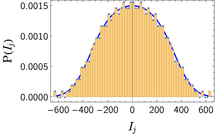
Figure 1: Normalized histogram for the distribution of integers for $L=N=512$ and the ”smooth” micro-state corresponding to a thermal macro-state with $c=\infty$, $\beta=0.1$ and $D=1$.

The rationale behind considering this state is that it can be scaled up in system size, which will allow us to consider the PDF of matrix elements between the smooth state and energy eigenstates belonging to the same or another macro-state.

III.1 Sampling micro-states for a given macro-state

As we are interested in statistical properties of matrix elements of local operators between energy eigenstates we require a method for randomly sampling given classes of eigenstates. This is a necessity because the number of micro-states corresponding to a given macro-state grows extremely rapidly with system size, cf. the discussion in section II. The basic principle is to sample the (half-odd) integers $I_{j}$ that specify micro-states in such a way that they are distributed according to the distribution function $\varrho(\nu)$ that defines the macro-state of interest. The difficulty is knowing how close the resulting histogram for a finite system of a few hundred particles should be to the thermodynamic limit distribution $\varrho(\nu)$ in order for a micro-state characterized by a set $\{I_{j}\}$ to “belong” to the macro-state defined by $\varrho(\nu)$. A detailed discussion of this issue and its resolution is given in Appendix B. The upshot is that we employ the following “simplified random sampling” algorithm:

1. Introduce a cutoff $I_{\rm max}$, define a set of (half-odd) integers $\mathfrak{S}=\{-I_{\rm max},-I_{\rm max}+1,\dots,I_{\rm max}\}$ and an empty set $S$.

2. Impose that the $I_{j}$ are distributed according to a PDF $P(\nu)$;

3. Determine the inverse $Z^{-1}(\nu)$ of the cumulative distribution function

   $$Z(\nu)=\int_{0}^{\nu}d\nu^{\prime}\ P(\nu^{\prime})\ ,\quad-\frac{1}{2}\leq Z(\nu)\leq\frac{1}{2}.$$ (42)

4. Generate a random number $|r|\leq\frac{1}{2}$ and use it to generate a random integer

   $$I={\rm Round}\big{(}LZ^{-1}(r)\big{)}.$$ (43)

5. We then update the sets $\mathfrak{S}$ and $S$ according to the rule

   $$\text{If }I\in\mathfrak{S}\land I\notin{S}$$

   $$\text{then }S\rightarrow S\cup\{I\}\ ,\ \mathfrak{S}\rightarrow\mathfrak{S}-\{I\}.$$ (44)

6. Repeat steps 4 and 5 until we arrive at a set $\{I_{1},\dots,I_{N}\}$ of distinct integers.

The PDF $P(\nu)$ is chosen such that this random sampling process on average reproduces the thermodynamic distribution $\varrho(\nu)$. We achieve this through an iterative numerical procedure. We show the resulting PDF for $T=10$, $D=1$ and $c=\infty$ in Fig. 2.

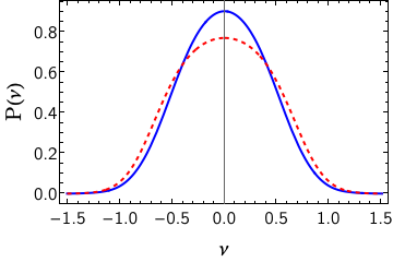
Figure 2: PDF $P(\nu)$ (solid blue line) and $\varrho(\nu)$ (dashed red line) for $T=10$, $D=1$ and $c=\infty$.

IV Local operators

Some representative spatially local operators in the Lieb-Liniger model are

• Density operator

  $$\rho(x)=\Phi^{\dagger}(x)\Phi(x)\ ,$$ (45)

• Interaction

  $$g_{2}(x)=\big{(}\Phi^{\dagger}(x)\big{)}^{2}\big{(}\Phi(x)\big{)}^{2}\ ,$$ (46)

• Bose field

  $$\Phi(x)\ .$$ (47)

As discussed earlier, in the limit $c\to\infty$ the model becomes equivalent to free fermions and in this limit additional local operators become of interest:

• Fermi field at $c=\infty$

  $$\Psi^{\dagger}(x)=\Phi^{\dagger}(x)\ e^{i\pi\int_{-\infty}^{x}dz\ \Phi^{\dagger}(z)\Phi(z)}\ ,$$ (48)

• Operator products involving the Fermi field at $c=\infty$, e.g.

  $$J_{n}(x) =(-i)^{n}\Psi^{\dagger}(x)\partial_{x}^{n}\Psi(x)\ ,$$

  $$F^{\dagger}_{n}(x) =\Psi^{\dagger}(x)\big{(}\partial^{n}_{x}\Psi^{\dagger}(x)\big{)}\Psi(x)\ .$$ (49)

All of the above operators are by construction spatially local (for finite values of $n$). However, in integrable models the existence of stable particle and hole excitations (at all energy densities) leads to an additional notion of locality. The stable excitations themselves have good spatial locality properties in the sense that they represent a local disturbance of the macro-state under consideration. It is then natural to ask whether a given local operator, say $\hat{\rho}(x)$, is local with respect to the operator that creates a local stable excitation. In relativistic integrable QFTs (at zero density) related notions of locality are known to have far-reaching consequences for matrix elements of local operators between energy eigenstates [30, 63].

In the impenetrable limit the situation becomes particularly simple. Here the elementary excitations are fermions and are created by $\Psi^{\dagger}(x)$. Operators like $\rho(x)$, $g_{2}(x)$, $J_{n}(x)$ and of course also $\Psi^{\dagger}(x)$ itself are local relative to $\Psi^{\dagger}(x)$ and in particular (anti)commute at a distance. On the other hand, the Bose field itself is not local relative to $\Psi^{\dagger}(x)$ as it involves a Jordan-Wigner like string operator. As is discussed below, this leads to a dramatic difference in the structure of matrix elements in energy eigenstates.

V Diagonal matrix elements of local operators in free theories

We first consider matrix elements of local operators in non-interacting theories. The naive expectation might be that these are trivial, but as we will see this is not the case for operators that are not local with respect to the elementary excitations. At $c=\infty$ energy eigenstates can be expressed as fermionic Fock states. Given a macro-state described by a root density $\rho(k)$ we can construct a corresponding micro-state $|\boldsymbol{k}\rangle=|k_{1},\dots,k_{N}\rangle$ following the procedure outlined in section III. Expectation values of local operators can then be straightforwardly calculated. Let us start with the single-fermion Green’s function at a fixed separation $x-y={\cal O}(L^{0})$

$$\langle\boldsymbol{k}|\Psi^{\dagger}(x)\Psi(y)|\boldsymbol{k}\rangle =\frac{1}{L}\sum_{p,q}\langle\boldsymbol{k}|\Psi^{\dagger}_{p}\Psi_{q}|\boldsymbol{k}\rangle\ e^{iyq-ipx}$$

$$=\int_{-\infty}^{\infty}dk\ e^{ik(y-x)}\rho(k)+o(L^{0}).$$ (50)

Importantly, up to finite-size corrections this only depends on the root density $\rho(k)$ characterizing the macro-state of interest. It is straightforward to extend this calculation to more complicated expectation values of the form

$$\langle\boldsymbol{k}|\Psi^{\dagger}(x_{1})\dots\Psi^{\dagger}(x_{n})\Psi(y_{n})\dots\Psi(y_{1})|\boldsymbol{k}\rangle\ ,$$ (51)

where we take $n$ to be fixed and all $x_{j}$ and all $y_{\ell}$ to lie in an interval of fixed size ${\cal O}(L^{0})$. Applying Wick’s theorem and using Eq. (50) we conclude that expectation values of any multi-point correlation function involving a fixed, finite number of fermion operators on a finite interval can be expressed solely in terms of the macro-state, up to finite size corrections. It then follows in turn that expectations values of any finite number of fermion operators calculated between different microstates corresponding to the same macro-state differ only by finite-size corrections that go to zero in the thermodynamic limit. Expectation values of local operators involving the Bose field at $c=\infty$ such as

$$\langle\boldsymbol{k}|\Phi^{\dagger}(x)\partial_{x}\Phi(x)|\boldsymbol{k}\rangle$$ (52)

can be obtained from these results by using the Bose-Fermi mapping as the latter involves only a finite number of Fermi fields. This is in contrast to expectation values like

$$\langle\boldsymbol{k}|\Phi^{\dagger}(x)\Phi(y)|\boldsymbol{k}\rangle=\langle\boldsymbol{k}|\Psi^{\dagger}(x)e^{i\pi\int_{y}^{x}dz\Psi^{\dagger}(z)\Psi(z)}\Psi(y)|\boldsymbol{k}\rangle\ ,$$ (53)

which can no longer be evaluated by using Wick’s theorem for a finite number of Fermi fields. This is intimately related to the fact that the Bose and Fermi fields are not mutually local. In order to assess how quickly the diagonal matrix elements approach their thermodynamic value with increasing $L$ we have considered the expectation values of the operators $J_{n}(0)$ (49) for $n=1,3$ in thermal micro-states $|\boldsymbol{k}\rangle$ at temperature $T=10$ and density $D=1$

$$\mathfrak{J}_{n}(\boldsymbol{k})=\langle\boldsymbol{k}|J_{n}(0)|\boldsymbol{k}\rangle$$ (54)

We determine the PDF of $\mathfrak{J}_{n}(\boldsymbol{k})$ when the thermal micro-states $|\boldsymbol{k}\rangle$ are sampled in a micro-canonical window $|E-e_{\infty}L|<10$, where $e_{\infty}$ is the thermal energy density in the thermodynamic limit and $E$ the energy eigenvalue of the micro-state. The PDFs are well described by normal distributions and their standard deviations as functions of system size are shown in Fig. 3.

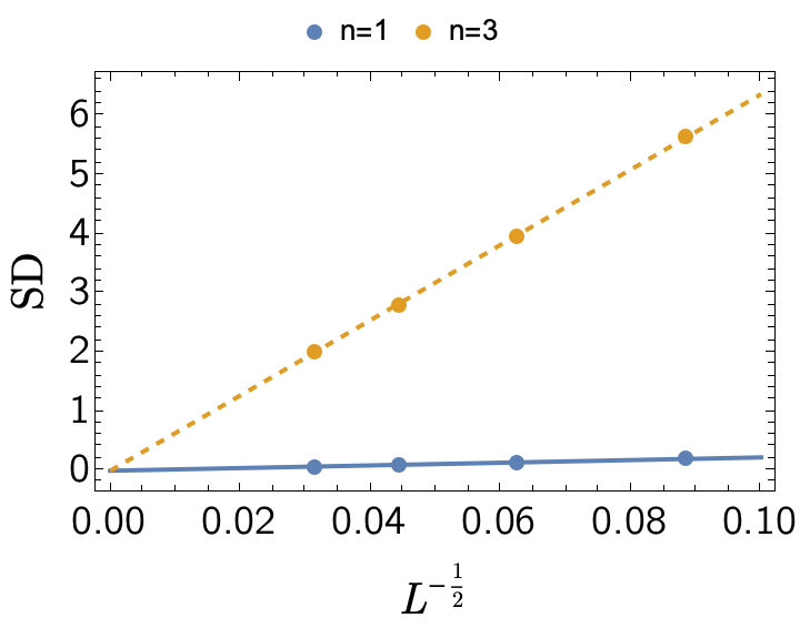
Figure 3: Standard deviations of the PDFs $P(\mathfrak{J}_{n}(\boldsymbol{k}))$ for $n=1,3$ and thermal micro-states $|\boldsymbol{k}\rangle$ at $T=10$, $D=1$ sampled in a micro-canonical window $|E-e_{\infty}L|<10$.

As the data is well described by simple linear fits we conclude that the standard deviations scale to zero as $L^{-1/2}$. This is in agreement with results on free theories in the literature [21].

VI Off-diagonal matrix elements in free theories

Our example for a free theory is again the $c=\infty$ limit of the Lieb-Liniger model. As we will see, the structure of off-diagonal matrix elements depends strongly on the locality properties of local operators ${\cal O}$ relative to the Fermi field $\Psi$. As before we consider $N$ particles on a ring of length $L$ and are interested in the thermodynamic limit $N,L\to\infty$ at fixed $D=N/L$.

VI.1 Local operators that are local relative to the Fermi field

The density operator $\rho(x)$ is spatially local as well as local with respect to the elementary fermion excitations of the Lieb-Liniger model at $c=\infty$. Let $|\boldsymbol{\lambda}\rangle$, $|\boldsymbol{\mu}\rangle$ be energy eigenstates with corresponding sets of (half-odd) integers $\{I_{j}\}$ and $\{J_{k}\}$. The matrix elements of the density operator vanish unless $\{I_{j}\}$ and $\{J_{k}\}$ differ by precisely one particle-hole excitation

$$\forall j\neq a\quad I_{j}=J_{j}\ ,\quad J_{a}=I_{a}+n\notin\{I_{j}\}.$$ (55)

For such one-particle-hole excitations we have the simple result

$$\frac{|\langle\boldsymbol{\mu}|\rho(0)|\boldsymbol{\lambda}\rangle|^{2}}{\langle\boldsymbol{\lambda}|\boldsymbol{\lambda}\rangle\langle\boldsymbol{\mu}|\boldsymbol{\mu}\rangle}\Bigg{|}_{\rm 1ph}=\frac{1}{L^{2}}\ .$$ (56)

If we introduce a cut-off $\Lambda$ in momentum the total number $N_{\rm ph}$ of states $|\boldsymbol{\mu}\rangle$ that lead to non-vanishing off-diagonal matrix elements scales polynomially with system size

$$N_{\rm ph}=N\Big{(}\frac{L\Lambda}{2\pi}-N\Big{)}.$$ (57)

The structure of matrix elements of other local operators that are mutually local with the Fermi field is analogous: only a very small fraction of all off-diagonal matrix elements are non-zero.

VI.2 Local operators that are not local relative to the Fermi field

As an example of a local operator that is not local relative to the Fermi field we consider the Bose field operator, which fulfils

$$\Phi(x)\Psi(y)=\text{sgn}(x-y)\Psi(y)\Phi(x)\ .$$ (58)

A convenient representation for the matrix elements of the Bose field operator at positive values of $c$ was derived in [33]. In the impenetrable limit the matrix element between a state $|\boldsymbol{\lambda}\rangle$ with $N$ particles and a state $|\boldsymbol{\mu}\rangle$ is non-vanishing only if the latter has $N-1$ particles and then reads

$$\frac{|\langle\boldsymbol{\mu}|\Phi(0)|\boldsymbol{\lambda}\rangle|^{2}}{\langle\boldsymbol{\lambda}|\boldsymbol{\lambda}\rangle\langle\boldsymbol{\mu}|\boldsymbol{\mu}\rangle}= \frac{2^{2N-2}}{L^{2N-1}}\prod_{j=1}^{N}\prod_{k=1}^{N-1}\frac{1}{(\lambda_{j}-\mu_{k})^{2}}$$

$$\times\prod_{j>k}^{N}(\lambda_{j}-\lambda_{k})^{2}\prod_{j>k}^{N-1}(\mu_{j}-\mu_{k})^{2}.$$ (59)

This result already shows that all matrix elements compatible with the simple particle number selection rule that $\Phi(0)$ changes particle number by one, are non-vanishing. This is in marked contrast to what we have for local operators that are local relative to the Fermi field.

VI.2.1 Matrix elements involving different macro-states

If $|\boldsymbol{\lambda}\rangle$ and $|\boldsymbol{\mu}\rangle$ belong to different macro-states, say with root densities $\rho_{0}(\lambda)$ and $\rho_{1}(\mu)$ respectively, it is straightforward to determine the leading contribution (in $L$) for large system sizes by noting that

$$\frac{1}{L^{2}}\ln\Big{[}\frac{|\langle\boldsymbol{\mu}|\Phi(0)|\boldsymbol{\lambda}\rangle|^{2}}{\langle\boldsymbol{\lambda}|\boldsymbol{\lambda}\rangle\langle\boldsymbol{\mu}|\boldsymbol{\mu}\rangle}\Big{]}=-\frac{1}{L^{2}}\sum_{j,k}\ln\big{(}\lambda_{j}-\mu_{k})^{2}$$

$$+\frac{1}{L^{2}}\sum_{j>k}^{N}\ln(\lambda_{j}-\lambda_{k})^{2}+\frac{1}{L^{2}}\sum_{j>k}^{N-1}\ln(\mu_{j}-\mu_{k})^{2}+o(L^{0}).$$ (60)

Turning sums into integrals this becomes

$$\frac{1}{L^{2}}\ln\Big{[}\frac{|\langle\boldsymbol{\mu}|\Phi(0)|\boldsymbol{\lambda}\rangle|^{2}}{\langle\boldsymbol{\lambda}|\boldsymbol{\lambda}\rangle\langle\boldsymbol{\mu}|\boldsymbol{\mu}\rangle}\Big{]}=\frac{1}{2}\int_{-\infty}^{\infty}d\lambda d\mu\ \big{[}\rho_{0}(\lambda)-\rho_{1}(\lambda)\big{]}\big{[}\rho_{0}(\mu)-\rho_{1}(\mu)\big{]}\ln\big{(}\lambda-\mu)^{2}+o(L^{0}).$$ (61)

This tells us that matrix elements involving two different macro-states are extremely small

$$\frac{|\langle\boldsymbol{\mu}|\Phi(0)|\boldsymbol{\lambda}\rangle|^{2}}{\langle\boldsymbol{\lambda}|\boldsymbol{\lambda}\rangle\langle\boldsymbol{\mu}|\boldsymbol{\mu}\rangle}\propto e^{-c_{\rho_{0},\rho_{1}}L^{2}}\ .$$ (62)

This behaviour is in stark contrast to the behaviour of off-diagonal matrix elements in different macro-states non-integrable models as predicted by the ETH. We note that the subleading terms (in system size) in (60) depend on the details of the micro-states $|\boldsymbol{\mu}\rangle$ and $|\boldsymbol{\lambda}\rangle$ and not only on the macro-state information encoded in $\rho_{0,1}(\lambda)$.

VI.2.2 Typical matrix elements in the same thermal macro-state

When $|\boldsymbol{\lambda}\rangle$ and $|\boldsymbol{\mu}\rangle$ belong to the same macro-state the leading (in $L$) term (62) vanishes as can be seen by taking $\rho_{1}(\lambda)=\rho_{0}(\lambda)$.

In order to understand the structure of the subleading terms we first fix $|\boldsymbol{\lambda}\rangle$ to correspond to a thermal state at temperature $T=10$ and density $D=1$ and then numerically determine the probability distribution of

$$\mathfrak{M}_{\boldsymbol{\lambda},\boldsymbol{\mu}}=-\frac{1}{L}\ln\Big{[}\frac{|\langle\boldsymbol{\mu}|\Phi(0)|\boldsymbol{\lambda}\rangle|^{2}}{\langle\boldsymbol{\lambda}|\boldsymbol{\lambda}\rangle\langle\boldsymbol{\mu}|\boldsymbol{\mu}\rangle}\Big{]}\ ,$$ (63)

where $|\boldsymbol{\mu}\rangle$ are micro-states corresponding to the same thermal macro-state and are taken to have energy eigenvalues such that $|E(\boldsymbol{\mu})-E(\boldsymbol{\lambda})|<25$. When $|\boldsymbol{\lambda}\rangle$ has $L$ rapidities, the states $|\mu\rangle$ must have $L-1$ particles in order for $\mathfrak{M}_{\boldsymbol{\lambda},\boldsymbol{\mu}}$ to be non-vanishing.

In Fig. 4, where we plot the probability distributions, obtained by sampling $\langle\boldsymbol{\mu}|$, for three different choices of the micro-state $|\boldsymbol{\lambda}\rangle$. Here all states belong to the same thermal macro-state with temperature $T=10$ and $L=N=512$.

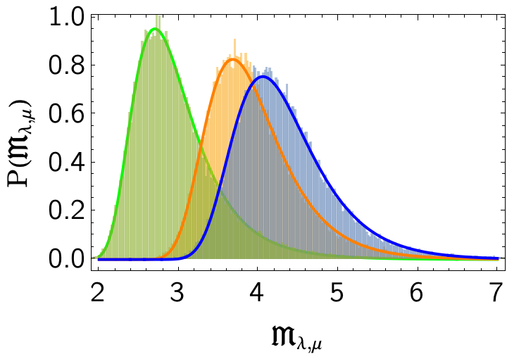
Figure 4: Normalized histograms of $|M_{\boldsymbol{\lambda},\boldsymbol{\mu}}|$ for three different micro-states $|\boldsymbol{\lambda}\rangle$ (see text) and 50000 states $|\boldsymbol{\mu}\rangle$ with $L=N=512$ (respectively in yellow, blue, green, red), where $|\boldsymbol{\lambda}\rangle$ and $|\boldsymbol{\mu}\rangle$ are micro-states corresponding to the thermal macro-state at temperature $T=10$.The solid lines are fits to Fréchet distribution functions.

We see that the probability distributions are very sensitive to the details of the micro-state $|\boldsymbol{\lambda}\rangle$, and not only on macro-state information encoded in $\rho_{0}(\lambda)$. The smallest mean value of ${\mathfrak{M}}_{\boldsymbol{\lambda},\boldsymbol{\mu}}$ (corresponding to the largest average absolute value of the matrix elements) is obtained when $|\boldsymbol{\lambda}\rangle$ corresponds to the smooth micro-state, cf. the green histogram in Fig. 1. The yellow histogram in Fig. 4, corresponding to the second-smallest mean of the distribution, is obtained by choosing a micro-state with the distribution of half-odd integers shown in Fig. 5.

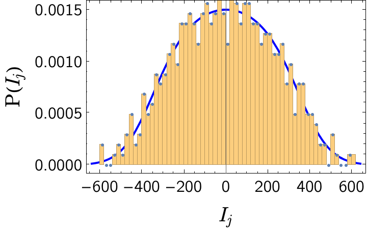
Figure 5: Normalized histogram for the distribution of integers for $L=N=512$ and a micro-state corresponding to a thermal macro-state with $c=\infty$, $\beta=0.1$ and $D=1$

We see that the distribution of integers in Fig. 5 does not reproduce the thermodynamic root density as well as the smooth state does. This notion can be quantified by computing the mean-squared distance between the histogram with bins $[\nu_{1},\dots,\nu_{n_{\rm bin}+1}]$

$$\Delta=\sum_{j=1}^{n_{\rm bin}}\Big{[}n_{j}-\int_{\nu_{j}}^{\nu_{j+1}}d\nu\frac{2\pi}{L}\rho\Big{(}\frac{2\pi}{L}\nu\Big{)}\Big{]}^{2}.$$ (64)

Here $n_{j}$ is the occupation of bin $j$ and $\rho(x)$ the thermodynamic root density describing the macro-state under consideration. The third micro-state considered in Fig. 4 (blue histogram) has the largest distance in this sense to the thermodynamic root density. This suggests that the larger the deviations of the root distribution of $|\boldsymbol{\lambda}\rangle$ from the thermodynamic root density are, the smaller the typical matrix elements $\mathfrak{M}_{\boldsymbol{\lambda},\boldsymbol{\mu}}$ (sampled over $\langle\boldsymbol{\mu}|$) become.

The solid lines in Fig. 4 are fits to Fréchet distribution functions

$$P_{\alpha,\beta,\nu}(x)=\begin{cases}(x-\nu)^{-\alpha-1}\exp\Big{[}-\big{(}\frac{x-\nu}{\beta}\big{)}^{-\alpha}\Big{]}&\text{if }x>\nu\\ 0&\text{else}.\end{cases}$$ (65)

We find that fits to $P_{\alpha,\beta,\nu}(x)$ provide excellent descriptions of our numerical PDFs in all cases we have considered. The parameters $\alpha,\beta,\nu$ depend not only on macro-state information, but on details of the micro-state $|\boldsymbol{\lambda}\rangle$, i.e.

$$\alpha=\alpha_{\boldsymbol{\lambda}}\ ,\quad\beta=\beta_{\boldsymbol{\lambda}}\ ,\quad\nu=\nu_{\boldsymbol{\lambda}}.$$ (66)

The next question we want to address is how the PDFs of $M_{\boldsymbol{\lambda},\boldsymbol{\mu}}$ scale with system size. To address this issue we work with the smooth state, because it can be readily scaled up with system size. We observe that we can achieve excellent data collapse if we shift the matrix elements by a $L$-dependent constant

$${M}_{\boldsymbol{\lambda},\boldsymbol{\mu}}=\mathfrak{M}_{\boldsymbol{\lambda},\boldsymbol{\mu}}-c_{0}\ln(L)\ .$$ (67)

In Fig. 6 we show the histograms of ${M}_{\boldsymbol{\lambda},\boldsymbol{\mu}}$ when sampled over the states $\langle\boldsymbol{\mu}|$ for a thermal macro-state with temperature $T=10$ and density $D=N/L=1$ for four different values of $L$ and $c_{0}=0.375801$. We observe that the data for different system sizes collapses very nicely.

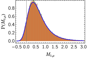
Figure 6: Normalized histograms of $M_{\boldsymbol{\lambda},\boldsymbol{\mu}}$ for the ”smooth” micro-state $|\boldsymbol{\lambda}\rangle$ (see text) and 50000 states $|\boldsymbol{\mu}\rangle$ with $L=N=128,256,512,1024$ (respectively in yellow, blue, green, red), where $|\boldsymbol{\lambda}\rangle$ and $|\boldsymbol{\mu}\rangle$ are micro-states corresponding to the thermal macro-state at temperature $T=10$. The solid line is a Fréchet distribution function with fitted parameters $\alpha=12.8894$, $\beta=5.04354$ and $\nu=-4.66742$.

Other micro-states are more difficult to scale up in system size, but supposedly an analogous data collapse of shifted distributions occurs.

In order to remove the explicit dependence of $P(M_{\boldsymbol{\lambda},\boldsymbol{\mu}})$ on the ket micro-state $|\boldsymbol{\lambda}\rangle$, we may sample the latter in the same energy window as the bra states $\langle\boldsymbol{\mu}|$. Denoting the energy density in the thermodynamic limit by $e_{\infty}$ we take this window to be $|E-Le_{\infty}|<7.5$. The resulting probability distributions of appropriately shifted matrix elements (67) is shown in Fig. 7 for a range of system sizes.

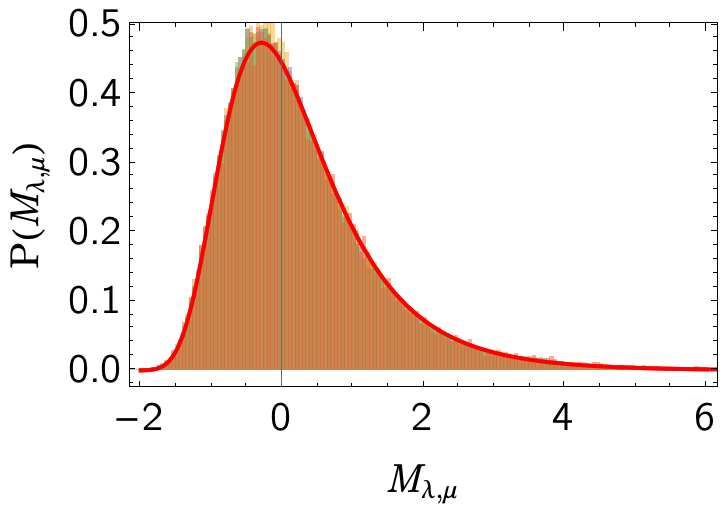
Figure 7: Normalized histograms of $M_{\boldsymbol{\lambda},\boldsymbol{\mu}}$ where both $|\boldsymbol{\lambda}\rangle$ and $|\boldsymbol{\mu}\rangle$ are sampled from a thermal macro-state at $T=10$, $D=1$ in a fixed energy window $|E-Le_{\infty}|<7.5$ with $L=N=64,128,256,512$ (respectively in yellow, blue, green and orange).The solid line is a Fréchet distribution function with fitted parameters $\alpha=13.0393$, $\beta=10.1444$ and $\nu=-10.3779$.

Fixing the constant in (67) to be $c_{0}=0.755474$ leads to an excellent data collapse, and the resulting probability distribution is again well described by a Fréchet distribution.

VI.2.3 Typical matrix elements in the same non-thermal macro-state

We have also considered typical matrix elements in atypical macro-states. As a particular example we present results for the distribution function of integers shown in Fig. 8.

Figure 8: Distribution function of $I_{j}/L$ for a non-thermal macro-state.

This corresponds to a generalized Gibbs ensemble with momentum distribution function

$$\rho(\lambda)=\frac{1}{2\pi\big{[}1+e^{(\lambda^{2}-\mu)/T+\mu_{3}\lambda^{4}+\mu_{4}\lambda^{6}}\big{]}}\ ,$$ (68)

where $T=20$, $\mu=32.0846$, $\mu_{3}=-0.01$, $\mu_{4}=0.00015$. The densities of energy and the fourth and sixth conservation law of the Lieb-Liniger model for this macro-state in the thermodynamic limit are respectively

$$e_{\infty}=32.0846\ ,\ \ q^{(4)}=1270.96\ ,\ \ q^{(6)}=55027.1\ .$$ (69)

In order to sample the macro-state we have chosen windows for the eigenvalues $|E-Le_{\infty}|<20$, $|\nu^{(4)}-Lq^{(4)}|<800$ and $|\nu^{(6)}-Lq^{(6)}|<34300$. We note that if we do not restrict the eigenvalues the probability distribution shifts by a small amount. The PDF of $M_{\boldsymbol{\lambda},\boldsymbol{\mu}}$, where both $|\boldsymbol{\lambda}\rangle$ and $|\boldsymbol{\mu}\rangle$ are sampled from the atypical macro-state constructed in this way and the constant shift is taken to be $c_{0}=0.680685$, is shown for a range of system sizes $64\leq N\leq 256$ in Fig. 9. We observe an excellent data collapse to a PDF that is well described by a Fréchet distribution function with fitted parameters $\alpha=8.99436$, $\beta=6.22114$ and $\nu=-6.50698$.

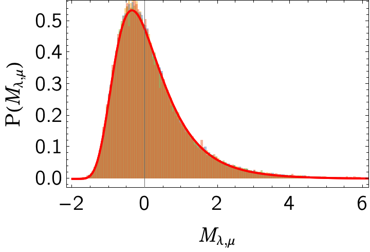
Figure 9: Normalized histograms of $M_{\boldsymbol{\lambda},\boldsymbol{\mu}}$ where both $|\boldsymbol{\lambda}\rangle$ and $|\boldsymbol{\mu}\rangle$ are sampled from the atypical macro-state described by the root density (68) in fixed windows of the energy and relevant higher conservation laws (see text) with $L=N=64,128,192,256$ (respectively in yellow, blue, green, orange).The solid line is a Fréchet distribution function with fitted parameters $\alpha=8.99436$, $\beta=6.22114$ and $\nu=-6.50698$.

Our results in this subsection can be summarized as follows.

• If we fix the ket state $|\boldsymbol{\lambda}\rangle$, then typical off-diagonal matrix elements in the same macro-state scale with system size as

  $$\frac{|\langle\boldsymbol{\mu}|\Phi(0)|\boldsymbol{\lambda}\rangle|^{2}}{\langle\boldsymbol{\lambda}|\boldsymbol{\lambda}\rangle\langle\boldsymbol{\mu}|\boldsymbol{\mu}\rangle}\propto e^{-c_{0}L\ln(L)-c_{1}L}\ .$$ (70)

  The corresponding probability distribution depends on details of $|\boldsymbol{\lambda}\rangle$, i.e. the multi-variate distribution function on (half-odd) integers and not only on macro-state information. In particular the two constants $c_{0,1}$ depend on the choice of $|\boldsymbol{\lambda}\rangle$.

• The probability distribution is well fitted by a Fréchet distribution, where the parameters depend on the choice of $|\boldsymbol{\lambda}\rangle$.

• If we sample both the bra and ket states over the same energy window typical matrix elements again scale with system-size as (70), and the resulting probability distribution is again well-fitted by a Fréchet distribution. In this case we expect $c_{0,1}$ to depend only on macro-state information.

An immediate consequence of the $e^{-c_{0}L\ln(L)}$ factor in (70) is that typical matrix elements will not contribute to correlation functions of local operators in the thermodynamic limit. To see this let us consider a two-point function in an energy eigenstate (generalized micro-canonical ensemble, cf. Ref. 64) corresponding to a macro-state characterized by the density $\varrho_{0}(z)$

$$F(x,t)=\langle\boldsymbol{\lambda}|\Phi^{\dagger}(x,t)\Phi(0,0)|\boldsymbol{\lambda}\rangle\ .$$ (71)

Employing a Lehmann representation and using the fact that matrix elements involving eigenstates corresponding to different macro-states $\varrho_{1}$ scale as $e^{-c_{\varrho_{0},\varrho_{1}}L^{2}}$, we have

$$F(x,t)= \sum_{\boldsymbol{\mu}}|\langle\boldsymbol{\lambda}|\Phi^{\dagger}(0,0)|\boldsymbol{\mu}\rangle|^{2}e^{-it(E_{\boldsymbol{\mu}}-E_{\boldsymbol{\lambda}})+ix(P_{\boldsymbol{\mu}}-P_{\boldsymbol{\lambda}})}$$

$$+o(L^{0})\ ,$$ (72)

where the sum is over all solutions to the Bethe ansatz equations that correspond to the macro-state characterized by $\varrho_{0}(z)$. Typical matrix elements cannot contribute to this sum because they scale with system size like (70), while their number scales as $e^{Ls_{\varrho_{0}}}$, where $s_{\varrho_{0}}$ is the thermodynamic entropy density of the macro-state under consideration. The spectral sum (72) must therefore be determined by ”anomalously large” matrix elements in the ”nose” of the probability distribution function. We turn to the question of how to characterize them next.

VI.2.4 Rare large matrix elements in the same macro-state

Which states $\langle\boldsymbol{\mu}|$ give anomalously large matrix elements $|\langle\boldsymbol{\mu}|\Phi(0,0)|\boldsymbol{\lambda}\rangle|$ for a a given ket state $|\boldsymbol{\lambda}\rangle|$? A natural guess is that each of the rapidities $\mu_{j}$ should be very close to one the rapidities $\lambda_{k}$ of the state $|\boldsymbol{\lambda}\rangle$, so that the factor $(\lambda_{k}-\mu_{j})^{-2}$ in the expression of the matrix-element (59) becomes very large. This intuition is indeed correct, as was shown for the case of the transverse-field Ising model in Ref. [65] (see also Refs [66, 67, 68]). In Fig. 10 we present histograms of matrix elements (63) for a smooth thermal state $|\boldsymbol{\lambda}\rangle$ at density $D=1$ and inverse temperature $\beta=0.1$ and a class of states $\langle\boldsymbol{\mu}|$ selected as follows:

• We randomly remove one of the rapidities in $\{\lambda_{1},\dots,\lambda_{N}\}$;

• In the remaining set we randomly shift each $\lambda_{j}$ by $\pm\pi/L$ under the constraint that all rapidities in the resulting set $\{\mu_{1},\dots,\mu_{N-1}\}$ must be different. In this way each $\mu_{n}$ is ”paired” with one of the $\lambda_{j}$ in the sense that their difference is as small as possible.

The set $\mathfrak{S}_{0}(\boldsymbol{\lambda})$ of states $\langle\boldsymbol{\mu}|$ constructed in this way is clearly exponentially large in system size. We may characterize $\mathfrak{S}_{0}(\boldsymbol{\lambda})$ in terms of a distance ($\lambda_{j}=2\pi I_{j}/L$, $\mu_{k}=2\pi J_{k}/L$)

$$d(\boldsymbol{\lambda},\boldsymbol{\mu})\equiv\displaystyle{{\text{min}}_{P\in S_{N}}}\sum_{j=1}^{N-1}(J_{j}-I_{P_{j}})^{2}\ ,$$ (73)

as the set of all eigenstates such that

$$d(\boldsymbol{\lambda},\boldsymbol{\mu})=\frac{N-1}{4}.$$ (74)

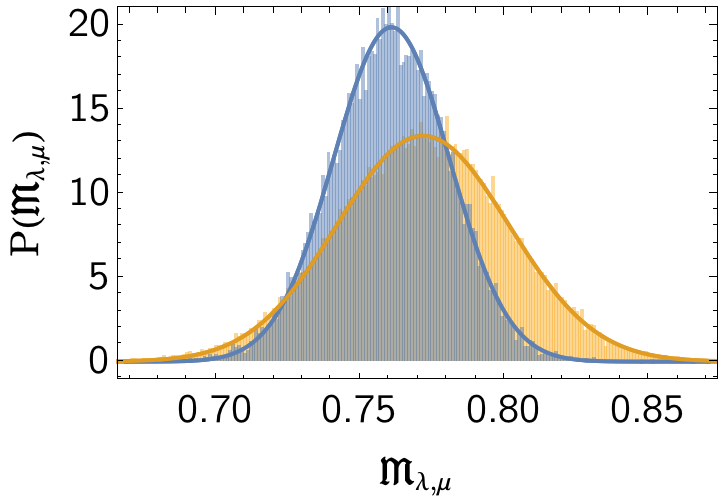
Figure 10: Normalized histograms of the matrix-elements of the field operator between a smooth thermal state with $D=1$ and $\beta=0.1$ and the atypical states in the set $\mathfrak{S}_{0}$ described in the text for $L=128$ (yellow) and $L=256$ (blue). The solid lines are fits to normal distributions.

We observe that the matrix elements for this class of states are indeed much larger than for typical thermal states, cf. Fig. 4. As the system size is increased the probability distribution narrows and shifts towards smaller values (i.e. large matrix elements). We find that $P(\mathfrak{M}_{\boldsymbol{\lambda},\boldsymbol{\mu}})$ is well described by a normal distribution.

While the matrix elements constructed in this way are large, their contribution to local correlation functions vanishes in the thermodynamic limit. This is most easily seen by considering the low density regime. Here the distance between neighbouring integers in a thermal state is typically much larger than $1$, which makes it easy to count states.

1. The number of states in $\mathfrak{S}_{0}(\boldsymbol{\lambda})$ is $N2^{N-1}$ in the low-density limit. The magnitude of the corresponding matrix elements with the smooth thermal state can be estimated as

   $$\mathfrak{M}_{\boldsymbol{\lambda},\boldsymbol{\mu}}\approx-D\ln\big{[}\frac{4}{\pi^{2}}\big{]}+\frac{\ln(L)}{L}-\frac{2\ln(\pi/2)}{L}.$$ (75)

   Hence

   $$\frac{|\langle\boldsymbol{\mu}|\Phi(0)|\boldsymbol{\lambda}\rangle|^{2}}{\langle\boldsymbol{\lambda}|\boldsymbol{\lambda}\rangle\langle\boldsymbol{\mu}|\boldsymbol{\mu}\rangle}\propto e^{LD\ln\big{[}\frac{4}{\pi^{2}}\big{]}}\ ,$$ (76)

   while the number of states in $\mathfrak{S}_{0}(\boldsymbol{\lambda})$ scales exponentially with system size

   $$|\mathfrak{S}_{0}(\boldsymbol{\lambda})|\propto e^{DL\ln(2)}.$$ (77)

   Concomitantly the contribution of such states to two-point functions vanishes in the thermodynamic limit as $e^{LD\ln(8/\pi^{2})}$.

2. We next consider the set of states $\mathfrak{S}_{1}$ that differs from $\mathfrak{S}_{0}$ by adding a single “soft mode”, by which we refer to one of the $J_{j}$ differing from its corresponding $I_{k}$ by $\pm(m+\frac{1}{2})$ rather than $\pm\frac{1}{2}$ (where we keep $m={\cal O}(L^{0})$). States in $\mathfrak{S}_{1}$ have

   $$d(\boldsymbol{\lambda},\boldsymbol{\mu})=\frac{N-1}{4}+\frac{(2m+1)^{2}-1}{4}.$$ (78)

   The same kind of argument as before now gives

   $$\mathfrak{M}_{\boldsymbol{\lambda},\boldsymbol{\mu}}\sim-D\ln\big{[}\frac{4}{\pi^{2}}\big{]}+\frac{\ln(L)}{L}+\frac{2\ln\big{(}\frac{2(2m+1)}{\pi}\big{)}}{L}.$$ (79)

   while the number of states increases to

   $$N(N-1)2^{N-1}.$$ (80)

   This shows that the contribution of such states to two-point functions again vanishes in the thermodynamic limit.

3. The above considerations generalize to a finite number of soft modes. The rare states of interest therefore involve an extensive number of soft modes, cf. Refs 65, 66, 67, 68. It was shown in Ref. [46] how to sum over soft modes in an arbitrary macro-state at low particle density and obtain an explicit expression for the single-boson Green’s function.

VII Matrix elements in interacting theories

The matrix elements of local operators between two normalized Bethe states have been derived in Refs  [31, 32, 33, 34]. In the case of the density operator the square of the matrix element between two normalized eigenstates $|\boldsymbol{\lambda}\rangle,|\boldsymbol{\mu}\rangle$ with respective numbers of Bethe roots $N,N^{\prime}$ reads

$$\frac{|\langle\boldsymbol{\lambda}|\hat{\rho}(0)|\boldsymbol{\mu}\rangle|^{2}}{\langle\boldsymbol{\lambda}|\boldsymbol{\lambda}\rangle\langle\boldsymbol{\mu}|\boldsymbol{\mu}\rangle}=\delta_{N,N^{\prime}}\frac{\left(\sum_{i=1}^{N}\mu_{i}-\lambda_{i}\right)^{2}}{L^{2N}\mathcal{N}_{\boldsymbol{\lambda}}\mathcal{N}_{\boldsymbol{\mu}}}\frac{\prod_{i\neq j}(\lambda_{i}-\lambda_{j})(\mu_{i}-\mu_{j})}{\prod_{i,j}(\lambda_{i}-\mu_{j})^{2}}\prod_{i\neq j}\frac{\lambda_{i}-\lambda_{j}+ic}{\mu_{i}-\mu_{j}+ic}$$ (81)

$$\times\left|\underset{i,j\neq p}{\det}\left[(V_{i}^{+}-V_{i}^{-})\delta_{ij}+i(\mu_{i}-\lambda_{i})\prod_{k\neq i}\frac{\mu_{k}-\lambda_{i}}{\lambda_{k}-\lambda_{i}}\left(\frac{2c}{(\lambda_{i}-\lambda_{j})^{2}+c^{2}}-\frac{2c}{(\lambda_{p}-\lambda_{j})^{2}+c^{2}}\right)\right]\right|^{2}\,.$$

Here $p\in\{1,...,N\}$ can be freely chosen,

$$V_{i}^{\pm}=\prod_{k=1}^{N}\frac{\mu_{k}-\lambda_{i}\pm ic}{\lambda_{k}-\lambda_{i}\pm ic}\,,$$ (82)

and $\mathcal{N}_{\boldsymbol{\lambda}}$ is given by

$$\mathcal{N}_{\boldsymbol{\lambda}}={\det}\left[\delta_{ij}\Big{(}1+\frac{1}{L}\sum_{k=1}^{N}\frac{2c}{c^{2}+\lambda_{i,k}^{2}}\Big{)}-\frac{1}{L}\frac{2c}{c^{2}+\lambda_{i,j}^{2}}\right]\,.$$ (83)

When presenting results for the statistic of such matrix elements we will consider logarithmic expressions like

$$\mathfrak{M}^{\rho}_{\boldsymbol{\lambda},\boldsymbol{\mu}}=-\frac{1}{L}\ln\Big{[}\frac{|\langle\boldsymbol{\mu}|\rho(0)|\boldsymbol{\lambda}\rangle|^{2}}{\langle\boldsymbol{\lambda}|\boldsymbol{\lambda}\rangle\langle\boldsymbol{\mu}|\boldsymbol{\mu}\rangle}\Big{]}\ .$$ (84)

In the following we also use the explicit expressions for the matrix elements of $g_{2}$ given in [34]. In the case $P_{\boldsymbol{\lambda}}\neq P_{\boldsymbol{\mu}}$ the following relation holds

$$\frac{|\langle\boldsymbol{\lambda}|g_{2}(0)|\boldsymbol{\mu}\rangle|^{2}}{\langle\boldsymbol{\lambda}|\boldsymbol{\lambda}\rangle\langle\boldsymbol{\mu}|\boldsymbol{\mu}\rangle}=\frac{|\langle\boldsymbol{\lambda}|\hat{\rho}(0)|\boldsymbol{\mu}\rangle|^{2}}{\langle\boldsymbol{\lambda}|\boldsymbol{\lambda}\rangle\langle\boldsymbol{\mu}|\boldsymbol{\mu}\rangle}\left(\frac{{\cal J}_{\boldsymbol{\lambda},\boldsymbol{\mu}}}{6c(P_{\boldsymbol{\lambda}}-P_{\boldsymbol{\mu}})^{2}}\right)^{2},$$ (85)

where

$${\cal J}_{\boldsymbol{\lambda},\boldsymbol{\mu}}= (P_{\boldsymbol{\lambda}}-P_{\boldsymbol{\mu}})^{4}-4(P_{\boldsymbol{\lambda}}-P_{\boldsymbol{\mu}})(\nu^{(3)}_{\boldsymbol{\lambda}}-\nu^{(3)}_{\boldsymbol{\mu}})$$

$$+3(E_{\boldsymbol{\lambda}}-E_{\boldsymbol{\mu}})^{2}.$$ (86)

The relation (85) has important consequences, because by construction we have

$$P_{\boldsymbol{\lambda}},E_{\boldsymbol{\lambda}},\nu^{(3)}_{\boldsymbol{\lambda}}\sim L\ .$$ (87)

This allows us to conclude that

$$\mathfrak{M}^{g_{2}}_{\boldsymbol{\lambda},\boldsymbol{\mu}}=\mathfrak{M}^{\rho}_{\boldsymbol{\lambda},\boldsymbol{\mu}}+{\cal O}\big{(}\frac{\ln(L)}{L}\big{)}\ ,$$ (88)

which means that up to finite-size corrections the statistical properties of $\mathfrak{M}^{g_{2}}_{\boldsymbol{\lambda},\boldsymbol{\mu}}$ and $\mathfrak{M}^{\rho}_{\boldsymbol{\lambda},\boldsymbol{\mu}}$ should be identical. We verify this by explicit numerical computations below.

VII.1 Diagonal matrix elements in interacting theories

In order to determine the statistical properties of diagonal matrix elements for $c<\infty$ we focus on the interaction potential $g_{2}(x)$ (46) because diagonal matrix elements of the density operator $\rho(x)$ are trivial due to particle number conservation. We further restrict our analysis to thermal macro-states. We determine the probability distribution of

$$\mathfrak{g}_{2}(\boldsymbol{\mu})=\frac{\langle\boldsymbol{\mu}|g_{2}(0)|\boldsymbol{\mu}\rangle}{\langle\boldsymbol{\mu}|\boldsymbol{\mu}\rangle}\ ,$$ (89)

where $|\boldsymbol{\mu}\rangle$ are thermal micro-states with energy $E_{\boldsymbol{\mu}}$, which we sample in an energy window $\omega=E_{\boldsymbol{\mu}}-E_{\rm smooth}\in[-50,50]$. Here $E_{\rm smooth}$ in the energy of the smooth thermal micro-state at a given temperature and system size. In Fig. 11 we show the resulting probability distribution for $T=10$, $L=512$ and $c=4$.

Figure 11: Probability distribution of $\mathfrak{g}_{2}(\boldsymbol{\mu})$ for thermal micro-states at $T=10$, $L=512$ and $c=4$, where we sample in an energy window as described in the main text.

As we increase the system size the average of the PDF converges as expected to the thermodynamic limit result. What is of interest is the scaling of the standard deviation of the PDF with system size. This is shown for three different values of $c$ and thermal micro-states at temperature $T=10$ and density $D=1$ in Fig. 12 for system sizes $L=64,128,256,512$. We see that the standard deviation collapses to zero. Motivated by the results in the $c=\infty$ limit we have fitted the date to second order polynomials in $x=L^{-\frac{1}{2}}$

$$f(x)=a_{1}x+a_{2}x^{2}\ .$$ (90)

The good quality of the fits suggests that for large system sizes the standard deviation scales as $L^{-1/2}$, as was previously observed for non-thermal states in the spin-1/2 XXZ chain [19] .

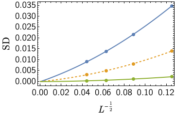
Figure 12: Standard deviations of $P(\mathfrak{g}_{2}(\boldsymbol{\mu}))$ for thermal micro-states at $T=10$, $D=1$ and at $c=1$ (blue), $c=4$ (yellow) and $c=16$ (green). The lines are fits as described in the main text.

The situation is very different in non-integrable models, where the scaling of the standard deviation is exponential in system size [7, 9, 8].

VII.2 Off-diagonal matrix elements in interacting theories

We now turn to our main topic of interest, off-diagonal matrix elements in interacting theories. We start by considering matrix elements of local operators between two different macro-states. On physical grounds these are expected to be very small and our aim is to ascertain their scaling with system size at a fixed density.

VII.2.1 Off-diagonal matrix elements between two different thermal macro states

Motivated by our results for matrix elements between two different macro states in the non-interacting case we examine the probability distributions of

$$\frac{1}{L}\mathfrak{M}^{\cal O}_{\boldsymbol{\lambda},\boldsymbol{\mu}} =\frac{1}{L^{2}}\ln\left(\frac{|\langle\boldsymbol{\mu}|{\cal O}(0)|\boldsymbol{\lambda}\rangle|^{2}}{\langle\boldsymbol{\lambda}|\boldsymbol{\lambda}\rangle\langle\boldsymbol{\mu}|\boldsymbol{\mu}\rangle}\right)\ ,\quad{\cal O}=\hat{\rho},\ g_{2}.$$ (91)

In particular we focus on the medians $m_{\cal O}$ and standard deviations $s_{\cal O}$ of the respective PDFs as functions of particle number $N$, which for simplicity is taken to be equal to $L$ throughout. We generate random samples of $1000$ micro-states $\langle\boldsymbol{\mu}|$ and $|\boldsymbol{\lambda}\rangle$ that belong to thermal macro-states at two different temperatures $T_{1}$ and $T_{2}$, and use them to numerically compute $20000$ matrix elements. Some results from this analysis are shown in Figs 13 (for $g_{2}$) and 14 (for $\hat{\rho}$).

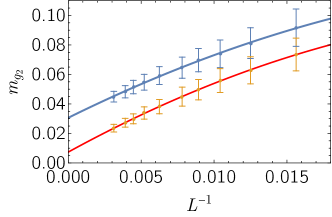
Figure 13: Medians (dots) $m_{g_{2}}$ and standard deviations $s_{g_{2}}$ (error bars) of the PDFs of $M^{g_{2}}_{\boldsymbol{\lambda},\boldsymbol{\mu}}/L$ where $|\boldsymbol{\lambda}\rangle$ and $|\boldsymbol{\mu}\rangle$ are sampled respectively from thermal macro-states at $T_{1}=10$, $T_{2}=5$ (blue symbols) and $T_{1}=10$, $T_{2}=7.5$ (red symbols) for $D=1$ in a fixed energy window $|E-Le_{\infty}|<25$. The solid lines are polynomial fits.

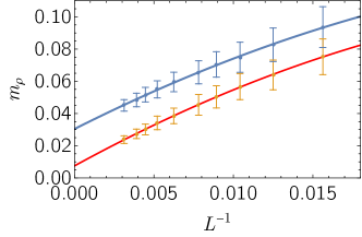
Figure 14: Same as Fig. 13 for matrix elements of the density operator $\hat{\rho}$.

We observe the following:

• The standard deviations of the PDFs narrow with increasing $L$;

• The medians $m_{g_{2}}$ and $m_{\rho}$ approach finite limiting values for large system sizes that depend on the macro-states but appear to be independent of which of the local operators $g_{2}(0)$ and $\hat{\rho}(0)$ we consider. Numerical extrapolations in $L^{-1}$ give limiting values that are close to value we obtained for the Bose field in the impenetrable case

  $$\frac{1}{L}\mathfrak{M}^{\cal O}_{\boldsymbol{\lambda},\boldsymbol{\mu}} \approx\frac{1}{2}\int_{-\infty}^{\infty}d\lambda d\mu\big{[}\rho_{0}(\lambda)-\rho_{1}(\lambda)\big{]}\big{[}\rho_{0}(\mu)-\rho_{1}(\mu)\big{]}$$

  $$\qquad\qquad\times\ \ln\big{(}\lambda-\mu)^{2}+o(L^{0}).$$ (92)

  Here $\rho_{0}(\lambda)$ and $\rho_{1}(\lambda)$ are the root densities of the two macro-states under considerations. The fact that the extrapolated values for $m_{g_{2}}$ and $m_{\rho}$ are the same is easy to understand from the explicit relation (85) between their matrix elements, which implies that for $P_{\boldsymbol{\lambda}}\neq P_{\boldsymbol{\mu}}$

  $$\frac{1}{L}\Big{[}\mathfrak{M}^{g_{2}}_{\boldsymbol{\lambda},\boldsymbol{\mu}}-\mathfrak{M}^{\hat{\rho}}_{\boldsymbol{\lambda},\boldsymbol{\mu}}\Big{]}=\frac{1}{L^{2}}\ln\left[\frac{{\cal J}_{\boldsymbol{\lambda},\boldsymbol{\mu}}^{2}}{6c(P_{\boldsymbol{\lambda}}-P_{\boldsymbol{\mu}})^{2}}\right]^{2}.$$ (93)

  The second term of the right-hand-side scales with system size as $\ln(L)/L^{2}$ and hence vanishes in the thermodynamic limit.

The results of this section are summarized as the following conjecture: matrix elements involving micro-states belonging to two different macro-states scale with system size as

$$\frac{|\langle\boldsymbol{\mu}|{\cal O}(0)|\boldsymbol{\lambda}\rangle|^{2}}{\langle\boldsymbol{\lambda}|\boldsymbol{\lambda}\rangle\langle\boldsymbol{\mu}|\boldsymbol{\mu}\rangle}\propto e^{-c^{\cal O}_{\rho_{0},\rho_{1}}L^{2}}\ .$$ (94)

Here $c^{\cal O}_{\rho_{0},\rho_{1}}$ is a constant that depends on the macro-states under consideration and a priori as well on the operator ${\cal O}$. The numerical results presented above are consistent with $c^{\cal O}_{\rho_{0},\rho_{1}}$ being independent of ${\cal O}$ and given by minus the right-hand-side of (92). This behaviour is in stark contrast to the behaviour of off-diagonal matrix elements in different macro-states non-integrable models as predicted by the ETH.

VII.3 Off-diagonal matrix elements between micro states belonging to the same thermal macro states

We now turn to matrix elements involving micro-states that belong to the same macro-state. The question we want to address is how the corresponding PDFs scale with system size. In order to remove the sensitive dependence on the ket micro-state we sample the ket states $|\boldsymbol{\lambda}\rangle$ over the same energy window as the bra state $\langle\boldsymbol{\mu}|$. Denoting the energy density in the thermodynamic limit by $e_{\infty}$ we take this window to be $|E-Le_{\infty}|<25$ in the figures shown below. For simplicity we focus on thermal macro-states. We observe that we can achieve excellent data collapse for the PDFs for different system sizes if we shift the matrix elements by a $L$-dependent constant

$${M}^{\cal O}_{\boldsymbol{\lambda},\boldsymbol{\mu}}=\mathfrak{M}^{\cal O}_{\boldsymbol{\lambda},\boldsymbol{\mu}}-c^{\cal O}_{0}\ln(L)\ ,\quad{\cal O}=\hat{\rho},g_{2}\ .$$ (95)

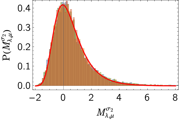
Figure 15: Normalized histograms of $M^{g_{2}}_{\boldsymbol{\lambda},\boldsymbol{\mu}}$ where both $|\boldsymbol{\lambda}\rangle$ and $|\boldsymbol{\mu}\rangle$ are sampled from a thermal macro-state at $T=5$, $D=1$ in a fixed energy window $|E-Le_{\infty}|<25$ with $L=N=64,96,160,224$ (respectively in yellow, blue, green and orange). The solid line is a Fréchet distribution function with fitted parameters $\alpha=16.1378$, $\beta=14.2188$ and $\nu=-14.2223$.

The resulting probability distributions of appropriately shifted matrix elements (67) of the interaction operator $g_{2}(0)$ in a thermal macro-state at $T=5$, $D=1$ is shown in Fig. 7 for $L=N=64,96,160,224$. Here we have fixed the constant in (67) to be $c^{\sigma_{2}}_{0}=0.754585$, which leads to a very good data collapse. The resulting probability distribution is well described by a Fréchet distribution with fitted parameters $\alpha=16.1378$, $\beta=14.2188$ and $\nu=-14.2223$.

The choice $c_{0}^{\rho}=c_{0}^{g_{2}}$ leads to a good data collapse, as shown in Fig. 6, and the resulting PDF is well described by a Fréchet distribution with fitted parameters $\alpha=17.3467$, $\beta=15.536$ and $\nu=-15.5163$.

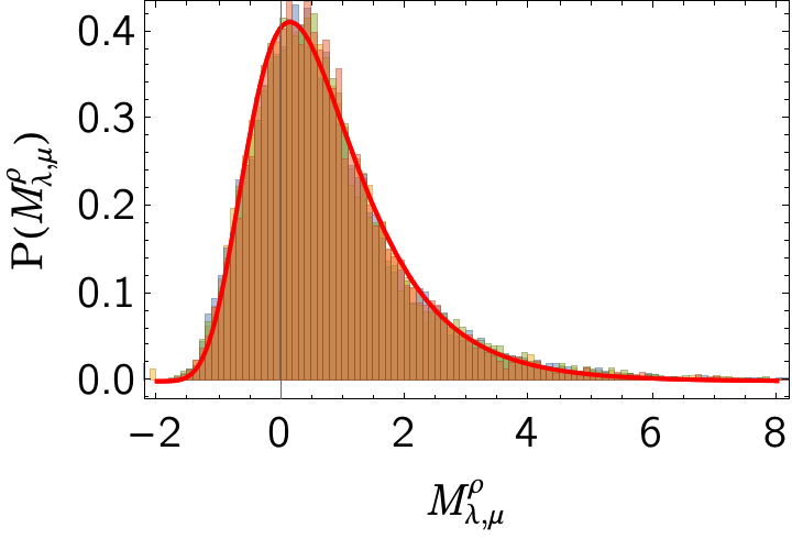
Figure 16: Normalized histograms of $M^{\rho}_{\boldsymbol{\lambda},\boldsymbol{\mu}}$ where both $|\boldsymbol{\lambda}\rangle$ and $|\boldsymbol{\mu}\rangle$ are sampled from a thermal macro-state at $T=5$, $D=1$ in a fixed energy window $|E-Le_{\infty}|<25$ with $L=N=64,96,160,224$ (respectively in yellow, blue, green and orange).The solid line is a Fréchet distribution function with fitted parameters $\alpha=17.3467$, $\beta=15.536$ and $\nu=-15.5163$.

The fact that the fitted Fréchet distributions differ slightly for $\hat{\rho}$ and $g_{2}$ is a result of the finite-size effects that scale as $\ln(L)/L$, cf. the discussion surrounding (88).

In Fig. 17 we show the probability distributions of appropriately shifted matrix elements (67) of the interaction operator $g_{2}(0)$ in a thermal macro-state at $T=10$, $D=1$ for $L=N=64,96,128,192,224$. Our choice of shift parameter $c^{g_{2}}=-0.995755$ is again seen to give a good data collapse for the histograms corresponding to different system sizes, and to be well described by a fitted Fréchet distribution.

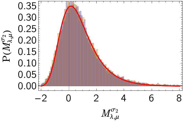
Figure 17: Normalized histograms of $M^{g_{2}}_{\boldsymbol{\lambda},\boldsymbol{\mu}}$ where both $|\boldsymbol{\lambda}\rangle$ and $|\boldsymbol{\mu}\rangle$ are sampled from a thermal macro-state at $T=10$, $D=1$ in a fixed energy window $|E-Le_{\infty}|<25$ with $L=N=64,96,128,192,224$ (respectively in yellow, blue, green, orange and purple). The solid line is a Fréchet distribution function with fitted parameters $\alpha=25.9405$, $\beta=27.2261$ and $\nu=-27.0405$.

The results of this subsection are summarized as the following conjecture: matrix elements involving micro-states belonging to the same macro-state scale with system size as

$$\frac{|\langle\boldsymbol{\mu}|{\cal O}(0)|\boldsymbol{\lambda}\rangle|^{2}}{\langle\boldsymbol{\lambda}|\boldsymbol{\lambda}\rangle\langle\boldsymbol{\mu}|\boldsymbol{\mu}\rangle}\propto e^{-c^{\cal O}_{0}L\ln(L)-LM^{\cal O}_{\boldsymbol{\lambda},\boldsymbol{\mu}}}\ ,$$ (96)

where $c^{\cal O}_{0}$ depends on the macro-states under consideration as well as (a priori) on the operator ${\cal O}$. The PDF for $M^{\cal O}_{\boldsymbol{\lambda},\boldsymbol{\mu}}$, where we sample both $\boldsymbol{\lambda}$ and $\boldsymbol{\mu}$, is well described by a Fréchet distribution.

VII.4 Atypically large matrix elements

As we have seen in the previous section, typical matrix elements of local operators scale with system size as (94) or (96). Even though there are exponentially many typical states, they cannot contribute to the Lehmann representation of two-point functions for the same reasons as discussed below eqn 72. Hence the matrix elements that matter in spectral representations must be in the “nose” of the PDF and concomitantly be atypically large and scale exponentially in system size. These involve Bethe states that differ by a finite number of “particle-hole” excitations of their associated (half-odd) integers. The example of a single particle-hole excitation is shown in Fig. 18. Given an eigenstate characterized by the set $\{I_{j}\}$ (shown as solid circles at the bottom) we construct an eigenstate characterized by $\{J_{j}\}$, obtained by changing a single half-odd integer $I_{a}$ (red empty circle) to $J_{a}$ (red solid circle).

Figure 18: Top: Bethe state that corresponds to a single particle-hole excitation over the micro-state with half-odd integers shown at the bottom.

Carrying out a finite number of particle-hole excitations leads to matrix elements that are atypically large. The PDF of matrix elements involving a single particle-hole excitations can be determined analytically in the large-$c$ limit, as we show next.

VII.4.1 Matrix elements of one-particle-hole states from a $1/c$-expansion

In Refs 45 and 55 it was shown how to carry out a $1/c$-expansion of 1-particle-hole and 2-particle-hole matrix elements. In order to address statistical properties of matrix elements we require higher orders in this expansion. In the following we carry out such an analysis for the 1-particle-hole matrix element of the density operator. Interestingly this reveals a novel ”infrared singularity”. We show that these contributions can be exponentiated, which in turn allows us to get an explicit expressions for the probability distribution of (the logarithm of) matrix elements in the thermodynamic limit.

Let $\boldsymbol{\lambda}$ and $\boldsymbol{\mu}$ be solutions to the Bethe Ansatz equations with corresponding sets of (distinct) integers $\{I_{j}\}$ and $\{J_{j}\}$ respectively, where

$$J_{j}=I_{j}\ ,\quad j\neq a\ ,\quad J_{a}=I_{a}+n.$$ (97)

This corresponds to a hole with integer $I_{a}$ (rapidity $\lambda_{a}$) and a particle with integer $I_{a}+n$ (rapidity $\mu_{a}$).

Figure 19: The set of (half-odd) integers $J_{j}$ (solid circles) corresponding to a single particle-hole excitation over a given microstate characterized by $\{I_{j}\}$: one (half-odd) integer is changed from $I_{a}$ (red empty circle) to $I_{a}+n$ (red solid circle).

The momentum difference between the two states is

$$P=\frac{2\pi n}{L}\ .$$ (98)

In the large-c limit the following expression for the 1-particle-hole matrix element of the density operator was derived in Ref. [55]

$$\frac{|\langle\boldsymbol{\lambda}|\hat{\rho}(0)|\boldsymbol{\mu}\rangle|^{2}}{\langle\boldsymbol{\lambda}|\boldsymbol{\lambda}\rangle\langle\boldsymbol{\mu}|\boldsymbol{\mu}\rangle}\Bigg{|}_{\text{1ph}}=\frac{\alpha^{2}}{(1+\frac{2}{cL})^{2}}\frac{1}{L^{2}}\Bigg{[}1+\frac{4P^{\prime}}{cL}\sum_{i\neq a}\Big{(}\frac{1}{\lambda_{i,a}-P^{\prime}}-\frac{1}{\lambda_{i,a}}\Big{)}+\frac{4P^{2}}{c^{2}L^{2}}\Bigg{(}-\frac{L^{2}}{12}\sum_{i\neq a}1+\sum_{\begin{subarray}{c}i\neq j\\ j\neq a\end{subarray}}\frac{1}{\lambda_{i,j}^{2}}$$

$$\hskip 142.26378pt+2\Big{(}\sum_{i\neq a}\frac{1}{\lambda_{i,a}-P^{\prime}}-\frac{1}{\lambda_{i,a}}\Big{)}^{2}+\sum_{i\neq a}\frac{1}{(\lambda_{i,a}-P^{\prime})^{2}}\Bigg{)}\Bigg{]}+{\cal O}(c^{-3})\ .$$ (99)

Here we have defined

$$\lambda_{i,j}=\lambda_{i}-\lambda_{j}\ ,\quad\alpha=1+\frac{2D}{c}\ ,\quad P^{\prime}=\frac{P}{\alpha}\ .$$ (100)

The leading term is $1/L^{2}$, but at ${\cal O}(c^{-2})$ there is in fact an infrared divergence

$$-\frac{DP^{2}}{3c^{2}L}+\frac{4P^{2}}{c^{2}L}\left[\frac{1}{L^{3}}\sum_{\begin{subarray}{c}i\neq j\\ i,j\neq a\end{subarray}}\frac{1}{\lambda_{i,j}^{2}}\right].$$ (101)

This contribution scales as $L^{-1}$ whereas the leading term in the $1/c$-expansion scales as $L^{-2}$. This suggests the following form for the matrix elements

$$\frac{|\langle\boldsymbol{\lambda}|\hat{\rho}(0)|\boldsymbol{\mu}\rangle|^{2}}{\langle\boldsymbol{\lambda}|\boldsymbol{\lambda}\rangle\langle\boldsymbol{\mu}|\boldsymbol{\mu}\rangle}\bigg{|}_{\text{1ph}}=\frac{h_{1}(\lambda_{a},P;\boldsymbol{\lambda})}{L^{2}}e^{-Lf_{1}(\lambda_{a},P;\boldsymbol{\lambda})}\ ,$$ (102)

where both $h_{1}$ and $f_{1}$ have regular expansions in $1/c$

$$f_{1}=\frac{a_{1}}{cL}+\frac{a_{2}}{c^{2}}+\ldots\ ,\quad h_{1}=1+\frac{b_{1}}{c}+\dots\ .$$ (103)

The leading terms in these expansions are then fixed by (VII.4.1) and in particular we have

$$a_{2}=\frac{DP^{2}}{3}-4P^{2}\int_{-\infty}^{\infty}d\mu\ \gamma_{-2}(\mu).$$ (104)

Here the pair distribution function $\gamma_{-2}(\mu)$ is defined as follows, cf. Ref. 45:

$$\lim_{L\to\infty}\frac{1}{L^{3}}\sum_{i\neq j}\frac{g(\lambda_{i},\lambda_{j})}{(\lambda_{i}-\lambda_{j})^{2}}=\int_{-\infty}^{\infty}d\lambda\ g(\lambda,\lambda)\gamma_{-2}(\lambda)\ ,$$ (105)

where $g(\lambda,\mu)$ is any smooth function. Importantly this quantity depends on details of the state $|\boldsymbol{\lambda}\rangle$ beyond its root density, namely the joint PDF of pairs of Bethe roots. The simplest way of determining it is by reverting to the sum in (101). The fact that expression for $a_{2}$ (104) involves the pair distribution function shows explicitly that the matrix elements (102) depend on details of the micro-state $|\boldsymbol{\lambda}\rangle$ beyond the macro-state information encoded in the particle root density.

In order to exhibit the structure (102) more fully we have determined the square of the 1-particle-hole matrix elements up to ${\cal O}(c^{-4})$ in Appendix A. Exponentiating the resulting infrared divergences using the conjecture (102) results in

$$\frac{|\langle\boldsymbol{\lambda}|\hat{\rho}(0)|\boldsymbol{\mu}\rangle|^{2}}{\langle\boldsymbol{\lambda}|\boldsymbol{\lambda}\rangle\langle\boldsymbol{\mu}|\boldsymbol{\mu}\rangle}\Bigg{|}_{\text{1ph,res}}\approx\frac{\alpha^{2}}{L^{2}\big{(}1+\frac{2}{cL}\big{)}^{2}}\Bigg{[}1-\frac{4P^{\prime}}{cL}\big{(}\Gamma_{-1}-\tilde{\Gamma}_{-1}\big{)}+\frac{8(P^{\prime})^{2}}{c^{2}L^{2}}\big{(}\Gamma_{-1}-\tilde{\Gamma}_{-1}\big{)}^{2}+\frac{4(P^{\prime})^{2}}{c^{2}L^{2}}\big{(}\Gamma_{-2}+\tilde{\Gamma}_{-2}\big{)}$$

$$\qquad-\frac{4\Gamma_{2}}{c^{3}L}-\frac{12P^{2}}{c^{3}L}+\frac{4P^{3}}{3c^{3}L}(\Gamma_{-1}-\tilde{\Gamma}_{-1})-\frac{16P^{3}}{3c^{3}L^{3}}\Big{[}2\big{(}\Gamma_{-1}-\tilde{\Gamma}_{-1}\big{)}^{3}+3\big{(}\Gamma_{-1}-\tilde{\Gamma}_{-1}\big{)}\big{(}\Gamma_{-2}+\tilde{\Gamma}_{-2}\big{)}+\big{(}\Gamma_{-3}-\tilde{\Gamma}_{-3}\big{)}\Bigg{]}$$

$$\qquad\times\exp\Big{[}-\frac{P^{2}(N-1)}{3c^{2}}+\frac{4(P^{\prime})^{2}}{c^{2}L^{2}}\sum_{\begin{subarray}{c}i\neq j\\ i,j\neq a\end{subarray}}\frac{1}{\lambda_{ij}^{2}}+\frac{4P^{2}D(N-1)}{c^{3}}-\frac{4PD\Gamma_{1}}{c^{3}}-\frac{8}{c^{3}L}\Big{(}\Gamma_{1}^{2}-N\Gamma_{2}\Big{)}\Big{]}.$$ (106)

Here we have introduced shorthand notations

$$\Gamma_{n}=\sum_{i\neq a}(\lambda_{i,a})^{n}\ ,\ \tilde{\Gamma}_{n}=\sum_{i\neq a}(\lambda_{i,a}-P^{\prime})^{n}\ .$$ (107)

We have verified numerically that the expression (VII.4.1) provides a good approximation to the exact matrix element at large values of $c$ in the regime $L>c$. This supports the conjecture (102). Some of this evidence is presented in Appendix A.

Comparing (VII.4.1) with (102) and dropping terms that vanish in the thermodynamic limit we have

$$f_{1}(\lambda_{a},P;\boldsymbol{\lambda}) =\frac{P^{2}D}{3c^{2}}-\frac{4{P^{\prime}}^{2}}{c^{2}L^{3}}\sum_{i\neq j}\frac{1}{\lambda_{ij}^{2}}-\frac{4P^{2}D^{2}}{c^{3}}$$

$$+\frac{4PD\Gamma_{1}}{Lc^{3}}+\frac{8}{c^{3}L^{2}}\Big{(}\Gamma_{1}^{2}-N\Gamma_{2}\Big{)}+\dots$$ (108)

In order to consider asymptotically large systems it is useful to express $f_{1}$ in terms of the particle and hole rapidities using

$$\lambda_{p}=\lambda_{h}+P^{\prime}\big{(}1+\frac{2}{cL}\big{)}+{\cal O}(c^{-3}).$$ (109)

Assuming for simplicity that the root distribution function $\rho(\lambda)$ of the rapidities $\boldsymbol{\lambda}$ is an even function from here on we have

$$f_{1}(\lambda_{h},\lambda_{p};\boldsymbol{\lambda}) =\frac{P^{2}}{c^{2}}\Big{[}\frac{D}{3}-\frac{4D^{2}}{c}-\frac{4}{\alpha^{2}}\int d\mu\ \gamma_{-2}(\mu)\Big{]}$$

$$-\frac{4D^{2}}{c^{3}}\lambda_{h}(\lambda_{p}-\lambda_{h})-\frac{8D}{c^{3}}\int d\mu\ \mu^{2}\ \rho(\mu)$$

$$+o(L^{0})\ .$$ (110)

Here we retain the label $\boldsymbol{\lambda}$ in order to indicate that $f_{1}$ depends on properties of the ket $|\boldsymbol{\lambda}\rangle$ beyond those encoded in its root density $\rho(\lambda)$. In the large-$L$ limit the logarithm of the matrix elements (84) for our one particle-hole excitation then becomes

$$\mathfrak{M}^{\rho}_{\boldsymbol{\lambda},\boldsymbol{\mu}}=f_{1}(\lambda_{h},\lambda_{p};\boldsymbol{\lambda})+o(L^{0})\ .$$ (111)

We now can determine the probability distribution $P(z,Q)$ of $\mathfrak{M}^{\rho}_{\boldsymbol{\lambda},\boldsymbol{\mu}}\Big{|}_{\rm 1ph}$ at a fixed momentum transfer $Q$ between the two states. To that end we introduce a rapidity cutoff $\Lambda$ that translates into a cutoff $I^{(L)}_{\rm max}$ for our Bethe integers, i.e. we consider only solutions of the Bethe equations such that all (half-odd) integers fulfil $|I_{j}|<I^{(L)}_{\rm max}$. We then define

$$P_{L}^{\eta}(z,Q)=\frac{1}{N_{1}}\!\sum_{I_{p},I_{h}}\delta_{\eta}(z-\mathfrak{M}^{\rho}_{\boldsymbol{\lambda},\boldsymbol{\mu}})\ \delta_{\eta}\big{(}Q-\frac{2\pi(I_{p}-I_{h})}{L}\big{)},$$ (112)

where $N_{1}$ is the total number of one particle-hole excitations given the state $|\boldsymbol{\lambda}\rangle$ and $I^{(L)}_{\rm max}$. We are interested in the joint PDF

$${\rm P}(z,Q)=\lim_{\eta\to 0}\lim_{L\to\infty}P_{L}^{\eta}(z,Q).$$ (113)

Turning sums into integrals in the thermodynamic limit gives

$${\rm P}(z,Q)=\frac{1}{{\cal N}_{\Lambda}}\int_{-\Lambda}^{\Lambda}d\lambda\ \rho(\lambda)\int_{-\Lambda}^{\Lambda}d{\mu}\ \rho_{h}(\mu)$$

$$\times\delta\big{(}z-f_{1}(\lambda,\mu;\boldsymbol{\lambda})\big{)}\ \delta\big{(}Q-2\pi[z(\mu)+z(\lambda)]\big{)}\ ,$$ (114)

where $z(\lambda)$ is the counting function defined in (31) and

$${\cal N}_{\Lambda}=\int_{-\Lambda}^{\Lambda}d\lambda\ \rho(\lambda)\int_{-\Lambda}^{\Lambda}d{\mu}\ \rho_{h}(\mu)\ .$$ (115)

In order to proceed we now use the approximation

$$2\pi[z(\mu)-z(\lambda)]=(\mu-\lambda)\alpha+{\cal O}(c^{-3}).$$ (116)

This allows us to carry out the integral over $\mu$ in an elementary fashion

$${\rm P}(z,Q)\approx\frac{1}{\alpha{\cal N}_{\Lambda}}\sum_{n}\frac{\rho_{p}(x_{n})\ \rho_{h}(x_{n}+Q/\alpha)}{|f^{\prime}_{1}(x_{n},x_{n}+Q/\alpha)|}\ ,$$ (117)

where the sum is over solutions $|x_{n}|<\Lambda$ to the equation

$$z-f_{1}(x_{n},x_{n}+Q/\alpha;\boldsymbol{\lambda})=0.$$ (118)

In our case there is only a single solution

$$x_{1}(z,Q) =-\frac{zc^{3}\alpha}{4D^{2}Q}-\frac{2\alpha}{DQ}\int d\mu\ \mu^{2}\rho(\mu)$$

$$+\frac{Qc}{4D^{2}\alpha}\Big{[}\frac{D}{3}-\frac{4D^{2}}{c}-\frac{4}{\alpha^{2}}\int d\mu\gamma_{-2}(\mu)\Big{]},$$ (119)

so that we arrive at a very simple answer

$${\rm P}(z,Q)\approx\frac{c^{3}}{4D^{2}{\cal N}_{\Lambda}}\frac{\rho(x_{1})\ \rho_{h}(x_{1}+Q/\alpha)}{|Q|}\ .$$ (120)

The probability distribution functions $P(z,Q=\pi)$ for smooth micro-states corresponding to a thermal macro-state with $D=0.25$, $\beta=0.25$ and two values of $c$ are shown in Fig. 20.

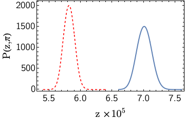
Figure 20: Probability distribution functions $P(z,Q=\pi)$ for smooth micro-states corresponding to thermal macro-states with $D=0.25$, $\beta=0.25$, $c=100$ (blue) and $c=110$ (red dashed).

We see that as expected the probability distribution function narrows and is peaked at smaller values of $z$ as $c$ is increased. In the limit $c\to\infty$ we know that $f_{1}\to 0$.

Here we have computed $\int d\mu\ \gamma_{-2}(\mu)$ by considering the scaling of its finite-size expression with $L$ for large systems of up to $L=4096$. It is important to stress that the thermodynamic limit result shown in Fig. 20 is approached only for very large $L$ such that $Lf_{1}\gg 1$. The results of this subsection are summarized as follows:

• Matrix elements involving a single-particle hole excitation over a given micro-state at a finite energy density relative to the ground state are exponentially small in system size

  $$\frac{|\langle\boldsymbol{\lambda}|\hat{\rho}(0)|\boldsymbol{\mu}\rangle|^{2}}{\langle\boldsymbol{\lambda}|\boldsymbol{\lambda}\rangle\langle\boldsymbol{\mu}|\boldsymbol{\mu}\rangle}\bigg{|}_{\text{1ph}}=\frac{h_{1}(\lambda_{a},P;\boldsymbol{\lambda})}{L^{2}}e^{-Lf_{1}(\lambda_{a},P;\boldsymbol{\lambda})}\ ,$$ (121)

  where the function $f_{1}$ has depends on details of the micro-state beyond the root density $\rho(\lambda)$ that specifies the macro-state to which it belongs. Above we have derived explicit expressions for the $1/c$-expansions of the functions $h_{1}$ and $f_{1}$.

• These matrix elements are very large compared to typical matrix elements in the same macro-state, which scale as (96).

• If we introduce a momentum cutoff there are only polynomially many (in system size) single particle-hole excitations, which means that they do not contribute to the thermodynamic limit of Lehmann representations of two-point functions for the same reasons as discussed below eqn 72.

VII.4.2 Multiple particle-hole excitations

We have verified numerically that making a fixed number of particle-hole excitations over a micro-state belonging to a thermal macro-state again leads to matrix elements that are exponentially small in system size. Hence such matrix elements are also anomalously large compared to typical ones. However, given a momentum cutoff there are only polynomially many (in system size) $m$-particle-hole excitations (where $m$ is fixed), which means that they do not contribute to the thermodynamic limit of Lehmann representations of two-point functions for the same reasons as discussed below eqn 72. The states that do contribute to such Lehmann representations involve an extensive number of particle-hole excitations.

VIII Summary and conclusions

In this work we have used integrability methods to determine the structure of matrix elements of local operators in energy eigenstates of the Lieb-Liniger model. The latter is a key paradigm of integrable many-particle quantum systems and has the distinctive property that energy eigenstates at an arbitrary energy density can be understood in terms of a single species of elementary excitations, which greatly simplifies the task of numerically determining matrix elements for large system sizes. The existence of an extensive number of mutually compatible conserved charges affects the structure of energy eigenstates at finite energy densities: in addition to thermal states we can have other macro-states that differ in their values of the densities of some of the conserved charges. Our results for the structure of matrix elements of local operators in the Lieb-Liniger model can be summarized as follows.

• Typical diagonal matrix elements in a macro-state characterized by a root density $\rho(\lambda)$ depend only on macro-state information up to finite-size corrections

  $$\frac{\langle\boldsymbol{\mu}|{\cal O}(0)|\boldsymbol{\mu}\rangle}{\langle\boldsymbol{\mu}|\boldsymbol{\mu}\rangle}=f_{\cal O}(\rho)+{\cal O}(L^{-\frac{1}{2}})\ .$$ (122)

  Here $f_{\cal O}(\rho)$ is a function that depends smoothly on the densities of the conserved charges. This can be thought of as a natural generalization of the eigenstate thermalization hypothesis for diagonal matrix elements. Our findings are in agreement with previous work on diagonal matrix elements in non-thermal states in the the spin-1/2 XXZ chain[19].

• Typical off-diagonal matrix elements involving micro-states belonging to two different macro-states scale with system size as

  $$\frac{|\langle\boldsymbol{\mu}|{\cal O}(0)|\boldsymbol{\lambda}\rangle|^{2}}{\langle\boldsymbol{\lambda}|\boldsymbol{\lambda}\rangle\langle\boldsymbol{\mu}|\boldsymbol{\mu}\rangle}\propto e^{-c^{\cal O}_{\rho_{0},\rho_{1}}L^{2}}\ .$$ (123)

  Here $c^{\cal O}_{\rho_{0},\rho_{1}}$ is a constant that depends on the macro-states under consideration and a priori as well on the operator ${\cal O}$.

• Typical off-diagonal matrix elements involving micro-states belonging to the same macro-state scale with system size as

  $$\frac{|\langle\boldsymbol{\mu}|{\cal O}(0)|\boldsymbol{\lambda}\rangle|^{2}}{\langle\boldsymbol{\lambda}|\boldsymbol{\lambda}\rangle\langle\boldsymbol{\mu}|\boldsymbol{\mu}\rangle}\propto e^{-c^{\cal O}_{0}L\ln(L)-LM^{\cal O}_{\boldsymbol{\lambda},\boldsymbol{\mu}}}\ ,$$ (124)

  where $c^{\cal O}_{0}$ depends on the macro-states under consideration as well as (a priori) on the operator ${\cal O}$. The PDF for $M^{\cal O}_{\boldsymbol{\lambda},\boldsymbol{\mu}}$, where we sample both $\boldsymbol{\lambda}$ and $\boldsymbol{\mu}$, is well described by a Fréchet distribution. If we fix the ket state $|\boldsymbol{\lambda}\rangle$ and consider the PDF of matrix elements obtained by sampling $|\boldsymbol{\mu}\rangle$ we observe a strong dependence on the details of $|\boldsymbol{\lambda}\rangle$, i.e. the multivariate probability distribution of half-odd integers. Nevertheless, if we fix $|\boldsymbol{\lambda}\rangle$ to be the smooth thermal state the PDF for $M^{\cal O}_{\boldsymbol{\lambda},\boldsymbol{\mu}}$ is well characterized by a Fréchet distribution (with different parameters compared to the case where we sample both $\boldsymbol{\lambda}$ and $\boldsymbol{\mu}$).

• There are rare, but still exponentially many (in particle number, given a momentum cut-off), matrix elements between eigenstates that belong to the same macro-state that are much larger than (124), but instead are merely exponentially small in system size

  $$\frac{|\langle\boldsymbol{\mu}|{\cal O}(0)|\boldsymbol{\lambda}\rangle|^{2}}{\langle\boldsymbol{\lambda}|\boldsymbol{\lambda}\rangle\langle\boldsymbol{\mu}|\boldsymbol{\mu}\rangle}\bigg{|}_{\rm rare}\propto e^{-LM^{\cal O}_{\boldsymbol{\lambda},\boldsymbol{\mu}}}\ .$$ (125)

  These can be characterized by the property that the sets of (half-odd) integers corresponding to the Bethe roots $\boldsymbol{\lambda}$ and $\boldsymbol{\mu}$ are atypically close to one another. For the case of the density operator we obtained explicit results for the simplest such matrix elements by generalizing the $1/c$-expansion method pioneered in Refs [45, 55].

• The observed structure of off-diagonal matrix elements in interacting theories is very similar to the one we find for the Bose field in the $c\to\infty$ limit, in which the Lieb-Liniger model can be mapped to free fermions. The origin of this similarity is the structure of the singularities of the matrix elements when viewed as functions of the spectral parameters (in a large finite volume the fact that the spectral parameters must fulfil the Bethe equations regularizes these singularities).

Our work poses a number of important questions that should be addressed in future work. First and foremost, it should be clarified whether the results obtained here indeed carry over to all local operators in the Lieb-Liniger model, and to other integrable models, as we conjecture. To that end it would be useful to consider non-thermal macro-states in the spin-1/2 XXZ chain as was done in [19] and check whether the same kind of scaling behaviour of matrix elements with system size reported here occurs. An analysis of the matrix elements of the Bose field in the Lieb-Liniger model for $0<c<\infty$ will be reported elsewhere [70]. Second, one should attempt to conduct an analogous study in models that feature bound states (string solutions to the Bethe equations). This appears difficult at present and will require a better control of matrix elements involving strings than is available in the literature. Third, the statistical properties of the rare, large matrix elements should be investigated in more detail in the case where one has a finite but low density of particle-hole excitations. Here the hope would be to find a way to randomly sample the large matrix elements that dominate the Lehmann representations of two-point functions and related quantities of interest [71].

Author contributions: FHLE conceptualized the work, carried out all calculations and computations and wrote the manuscript. AJJMdK worked on carrying out numerical calculations for the interacting case and analyzing the associated results.

Appendix A $1/c$-expansion of the 1-particle-hole matrix element

In this Appendix we present some details regarding the $1/c$-expansion of the density matrix element (84) between two Bethe states differing by a single particle-hole excitation, cf. section VII.4.1 of the main text. For convenience we first recall some of the notations introduced in the main text. We consider two solutions $\boldsymbol{\lambda}$ and $\boldsymbol{\mu}$ to the Bethe Ansatz equations with corresponding sets of (distinct) integers $\{I_{j}\}$ and $\{J_{j}\}$, where

$$J_{j}=I_{j}\ ,\quad j\neq a\ ,\quad J_{a}=I_{a}+n.$$ (126)

This corresponds to a hole with integer $I_{a}$ (rapidity $\lambda_{a}$) and a particle with integer $I_{a}+n$ (rapidity $\mu_{a}$). The momentum difference between the two states is $P=2\pi n/L$. In order to simply the expression for the matrix element in the $1/c$-expansion it is useful to introduce short-hand notations

$$\lambda_{i,j} =\lambda_{i}-\lambda_{j}\ ,\quad\alpha=1+\frac{2D}{c}\ ,\quad P^{\prime}=\frac{P}{\alpha}\ ,$$

$$\Gamma_{n} =\sum_{i\neq a}(\lambda_{i,a})^{n}\ ,\ \tilde{\Gamma}_{n}=\sum_{i\neq a}(\lambda_{i,a}-P^{\prime})^{n}\ .$$ (127)

Solving the Bethe equations in the framework of the $1/c$-expansion gives

$$\lambda_{i}= \frac{2\pi I_{i}}{\alpha L}+\frac{4\pi}{cL^{2}\alpha}\sum_{j=1}^{N}I_{j}+\frac{(2\pi)^{4}}{3\pi c^{3}(\alpha L)^{4}}\sum_{j=1}^{N}\left({I_{i}-I_{j}}\right)^{3}$$

$$+{\cal O}(c^{-4})\,.$$ (128)

We then can express the rapidities $\mu_{k}$ in terms of the $\lambda_{j}$ as

$$\mu_{i}= \lambda_{i}+\frac{2P^{\prime}}{cL}\left[1-\frac{(\lambda_{i,a})^{2}}{c^{2}}+\frac{P\lambda_{i,a}}{c^{2}}-\frac{P^{2}}{3c^{2}}\right]+{\cal O}(c^{-4})\ ,$$

$$\mu_{a}= \lambda_{a}+P^{\prime}\left[1+\frac{2}{cL}\right]+\frac{2}{3c^{3}L}\sum_{k\neq a}\left[(\lambda_{a,k}+P)^{3}-\lambda_{a,k}^{3}\right]$$

$$+{\cal O}(c^{-4})\ .$$ (129)

We now extend the analysis of Ref. [45] by carrying out a $1/c$-expansion of the various factors in the expression (81) of the matrix elements of th density operator up to order ${\cal O}(c^{-4})$. As in [45] we retain certain contributions to all orders. We find

$$A_{1}\equiv\prod_{i\neq j}\frac{\lambda_{i,j}+ic}{\mu_{i,j}+ic}\simeq 1-\frac{{P^{\prime}}^{2}(N-1)}{c^{2}}+\frac{2P^{\prime}}{c^{2}}\Gamma_{1}(\lambda_{a}),$$

$$A_{2}\equiv\Big{|}\prod_{i\neq a}(V_{i}^{+}-V_{i}^{-})\Big{|}^{2}\simeq\Big{(}\frac{2P}{c}\Big{)}^{2N-2}\Big{(}1-\frac{2}{c^{2}}\Gamma_{2}(\lambda_{a})\Big{)},$$

$$A_{3}\equiv\prod_{\begin{subarray}{c}i\neq j\\ i\neq a\\ j\neq a\end{subarray}}\frac{\lambda_{i,j}\mu_{i,j}}{(\lambda_{i}-\mu_{j})^{2}}\simeq 1+\frac{4{P^{\prime}}^{2}}{c^{2}L^{2}}\sum_{\begin{subarray}{c}i\neq j\\ i\neq a\\ j\neq a\end{subarray}}\frac{1}{\lambda_{i,j}^{2}},$$

$$\mathcal{N}_{\boldsymbol{\lambda}}\simeq\alpha^{N-1}\Big{[}1+\frac{4}{c^{3}L}\Big{(}\big{(}\sum_{i}\lambda_{i}\big{)}^{2}-N\sum_{i}\lambda_{i}^{2}\Big{)}\Big{]},$$

$$\mathcal{N}_{\boldsymbol{\mu}}\simeq\mathcal{N}_{\boldsymbol{\lambda}}\Big{[}1+\frac{4P}{c^{3}L}\big{(}2\Gamma_{1}(\lambda_{a})-(N-1)P\big{)}\Big{]},$$ (130)

$$A_{4}\equiv\prod_{i\neq a}\frac{\lambda_{i,a}^{2}}{(\mu_{i}-\lambda_{a})^{2}}\simeq 1-\frac{4P^{\prime}}{cL}\Gamma_{-1}+\frac{8{P^{\prime}}^{2}}{c^{2}L^{2}}\Big{[}\Gamma_{-1}^{2}+\frac{\Gamma_{-2}}{2}\Big{]}$$

$$\hskip 62.59596pt-\frac{16P^{3}}{3c^{3}L^{3}}\Big{[}2\Gamma_{-1}^{3}+3\Gamma_{-1}\Gamma_{-2}+\Gamma_{-3}\Big{]}$$

$$\hskip 62.59596pt+\frac{4P}{c^{3}L}\Big{[}\Gamma_{1}-3P+\frac{P^{2}\Gamma_{-1}}{3}\Big{]}.$$ (131)

$$A_{5}\equiv\prod_{i\neq a}\frac{(\mu_{i}-\mu_{a})^{2}}{(\lambda_{i}-\mu_{a})^{2}}\simeq 1+\frac{4P^{\prime}}{cL}\big{(}1-\frac{P^{2}}{3c^{2}}\big{)}\tilde{\Gamma}_{-1}$$

$$\hskip 48.36958pt+\frac{4{P^{\prime}}^{2}}{c^{2}L^{2}}\Big{[}2\tilde{\Gamma}_{-1}^{2}+\tilde{\Gamma}_{-2}\Big{]}-\frac{4P}{Lc^{3}}\Gamma_{1}$$

$$\hskip 48.36958pt+\frac{16P^{3}}{3c^{3}L^{3}}\Big{[}2\tilde{\Gamma}_{-1}^{3}+3\tilde{\Gamma}_{-2}\tilde{\Gamma}_{-1}+\tilde{\Gamma}_{-3})\Big{]},$$ (132)

$$A_{6}\equiv\prod_{i=1}^{N}\frac{1}{(\lambda_{i}-\mu_{i})^{2}}\simeq\frac{\alpha^{2N}}{P^{2}}\left(\frac{Lc}{2P}\right)^{2N-2}$$

$$\times\Big{[}1+\frac{2}{c^{2}}\big{(}\Gamma_{2}-P\Gamma_{1}+\frac{P^{2}}{3}(N-1)\big{)}\big{(}1-\frac{2}{cL}\big{)}\Big{]},$$ (133)

Finally we have

$$i(\mu_{l}-\lambda_{l})\prod_{k\neq l}\frac{\mu_{k}-\lambda_{l}}{\lambda_{k}-\lambda_{l}}\Big{[}\frac{2c}{\lambda_{l,j}^{2}+c^{2}}-\frac{2c}{(\lambda_{p,j}^{2}+c^{2}}\Big{]}\simeq 0,$$

$$\Big{(}\sum_{i}\mu_{i}-\lambda_{i}\Big{)}^{2}\simeq P^{2}\ .$$ (134)

The leading corrections in (130)-(134) are of order ${\cal O}(c^{-4})$. Substituting the results back into the expression (84) for the matrix elements leads to the following expression for one states that differ by a single particle-hole excitation

$$\frac{|\langle\boldsymbol{\lambda}|\hat{\rho}(0)|\boldsymbol{\mu}\rangle|^{2}}{\langle\boldsymbol{\lambda}|\boldsymbol{\lambda}\rangle\langle\boldsymbol{\mu}|\boldsymbol{\mu}\rangle}\bigg{|}_{\text{1ph}}=\frac{\alpha^{2}}{L^{2}\big{(}1+\frac{2}{cL}\big{)}^{2}}\Bigg{[}1-\frac{4P^{\prime}}{cL}\big{(}\Gamma_{-1}-\tilde{\Gamma}_{-1}\big{)}-\frac{P^{2}(N-1)}{3c^{2}}+\frac{4{P^{\prime}}^{2}}{c^{2}L^{2}}\sum_{i\neq j}\frac{1}{\lambda_{ij}^{2}}+\frac{8{P^{\prime}}^{2}}{c^{2}L^{2}}\big{(}\Gamma_{-1}-\tilde{\Gamma}_{-1}\big{)}^{2}$$

$$+\frac{4{P^{\prime}}^{2}}{c^{2}L^{2}}\big{(}\Gamma_{-2}+\tilde{\Gamma}_{-2}\big{)}+\frac{4P^{3}N}{3c^{3}L}\big{(}\Gamma_{-1}-\tilde{\Gamma}_{-1}\big{)}+\frac{4P^{2}D(N-1)}{c^{3}}-\frac{4PD\Gamma_{1}}{c^{3}}-\frac{4\Gamma_{2}}{c^{3}L}-\frac{8}{c^{3}L}\Big{(}\big{(}\sum_{i}\lambda_{i}\big{)}^{2}-N\sum_{i}\lambda_{i}^{2}\Big{)}-\frac{12P^{2}}{c^{3}L}$$

$$-\frac{16P^{3}}{3c^{3}L^{3}}\Big{[}2\big{(}\Gamma_{-1}-\tilde{\Gamma}_{-1}\big{)}^{3}+3\big{(}\Gamma_{-1}-\tilde{\Gamma}_{-1}\big{)}\big{(}\Gamma_{-2}+\tilde{\Gamma}_{-2}\big{)}+\big{(}\Gamma_{-3}-\tilde{\Gamma}_{-3}\big{)}\Big{]}-\frac{16P^{3}}{c^{3}L^{3}}\big{(}\Gamma_{-1}-\tilde{\Gamma}_{-1}\big{)}\sum_{i\neq j}\frac{1}{\lambda_{ij}^{2}}\Bigg{]}+{\cal O}(c^{-4})\ .$$ (135)

This expression indeed exhibits “infrared divergences”, i.e. contributions that acquire additional factors of $L$ compared to the leading term, that are compatible with the conjecture (102). We conjecture that these terms can be exponentiated and in order to do so it is useful to return to the individual factors they arise from

$$A_{1} \approx A_{1}^{\text{(r)}}=\exp\Big{(}-\frac{{P^{\prime}}^{2}(N-1)}{c^{2}}+\frac{2P^{\prime}}{c^{2}}\Gamma_{1}\Big{)}\ ,$$

$$A_{2} \approx A_{2}^{\text{(r)}}=\Big{(}\frac{2P}{c}\Big{)}^{2N-2}\exp\Big{(}-\frac{2}{c^{2}}\Gamma_{2}\Big{)},$$

$$A_{3} \approx A_{3}^{\text{(r)}}=\exp\bigg{(}\frac{4{P^{\prime}}^{2}}{c^{2}L^{2}}\sum_{\begin{subarray}{c}i\neq j\\ i,j\neq a\end{subarray}}\frac{1}{\lambda_{i,j}^{2}}\bigg{)}\ ,$$

$$\mathcal{N}_{\boldsymbol{\lambda}} \approx\mathcal{N}^{\text{(r)}}_{\boldsymbol{\lambda}}=\alpha^{N-1}\exp\Big{(}\frac{4}{c^{3}L}\big{(}\Gamma_{1}^{2}-N\Gamma_{2}\big{)}\Big{)}\ ,$$ (136)

$$A_{6} \approx A_{6}^{\text{(r)}}=\frac{\alpha^{2N}}{P^{2}\big{(}1+\frac{2}{cL}\big{)}^{2}}\left(\frac{Lc}{2P}\right)^{2N-2}$$

$$\times\exp\Big{(}\frac{2}{c^{2}}\big{(}\Gamma_{2}-P\Gamma_{1}+\frac{P^{2}}{3}(N-1)\big{)}\big{(}1-\frac{2}{cL}\big{)}\Big{)}.$$ (137)

Using (136), (137) to exponentiate the infrared singularities in (A) results in the expression (VII.4.1) in the main text. In order to assess the accuracy of (VII.4.1) we have computed its ratio $R$ to numerically exact matrix elements for a number of particle-hole excitations over a ”smooth” thermal state with $\beta=1$, where

$$R=\frac{|\langle\boldsymbol{\lambda}|\hat{\rho}(0)|\boldsymbol{\mu}\rangle|^{2}}{\langle\boldsymbol{\lambda}|\boldsymbol{\lambda}\rangle\langle\boldsymbol{\mu}|\boldsymbol{\mu}\rangle}\bigg{|}_{\text{1ph,res}}\bigg{(}\frac{|\langle\boldsymbol{\lambda}|\hat{\rho}(0)|\boldsymbol{\mu}\rangle|^{2}}{\langle\boldsymbol{\lambda}|\boldsymbol{\lambda}\rangle\langle\boldsymbol{\mu}|\boldsymbol{\mu}\rangle}\bigg{|}_{\text{1ph}}\bigg{)}^{-1}.$$ (138)

For the same states we have also checked the accuracy of the exponentiations (136), (137). Results for $L=N=128$ and $c=100$ are shown in Table 1

P	$2J_{a}$	$2I_{a}$	${A^{(r)}_{1}}/{A_{1}}$	$A^{\rm(r)}_{2}/A_{2}$	$A^{\rm(r)}_{3}/A_{3}$	$A^{\rm(r)}_{6}/A_{6}$	$R$
-5.15	-287	-77	0.998	1.00	1.03	0.995	1.022
-3.14	-261	-133	0.999	1.00	1.02	0.991	1.014
5.35	223	5	0.999	1.00	1.02	1.	1.018
-4.47	-173	9	1.00	1.00	1.01	1.	1.013
4.57	207	21	0.999	1.00	1.01	1.00	1.015
-2.85	-155	-39	1.00	1.00	1.01	1.	1.009
-6.92	-243	39	0.999	1.00	1.02	1.	1.025
6.97	273	-11	0.998	1.00	1.02	1.00	1.027
-6.38	-225	35	0.999	1.00	1.02	1.	1.021
-4.61	219	-31	0.999	1.00	1.02	1.	1.016

Table 1: Results for the ratios of the resummed $1/c$-expansions for matrix elements to the numerically exact results for $c=100$, $L=N=128$, $\beta=1$. We see that the resummed expression works rather well. As expected it does become worse when the excited state involves larger differences $|\lambda_{p}-\lambda_{h}|$ as the $1/c$-expansion requires these to be small compared to $c$.

We see that the results are quite satisfactory. The values of $\beta$ and $c$ have been chosen to ensure that the differences $|\lambda_{j,k}|$ are all small compared to $c$, which is a key assumption of the $1/c$-expansion, cf. the discussion in Ref. [45]. We note that the factors $A^{\text{(r)}}_{n}$ are generally quite different from their ”bare” values, which indicates the breakdown of the bare $1/c$-expansion. However, in the final expression (VII.4.1) a number of cancellations occur, which render the resummed result (VII.4.1) very close to the bare expression (A) for the parameters considered here.

Appendix B Sampling macro-states in a finite volume

In this appendix we discuss in some detail how to sample a given macro-state for a large, finite number of particles. The key element is to generate appropriate sets of “Bethe integers” $I_{j}$, which characterize the solutions of the Bethe equations (27). For simplicity we focus on the impenetrable case $c=\infty$, where

$$\lambda_{j}=\frac{2\pi I_{j}}{L}\ .$$ (139)

Thermal states are of particular interest as they are the most abundant states at a given energy density and we therefore focus on them in our discussion. The generalization to atypical finite entropy states is straightforward. To be specific we take $c=\infty$ and consider a temperature $T=10$ and chemical potential $\mu=12.1058$. This gives particle density $D=1$, energy density

$$e_{\infty}=8.036608362699118\ ,$$ (140)

and a root density

$$\rho(x)=\frac{1}{2\pi}\frac{1}{1+e^{(x^{2}-\mu)/T}}\ .$$ (141)

The corresponding density of $I_{j}/L$ is simply

$$\varrho(\nu)=\frac{1}{1+e^{((2\pi\nu)^{2}-\mu)/T}}\ .$$ (142)

For later convenience we define a cumulative probability distribution function

$$C(\nu)=\frac{1}{D}\int_{0}^{\nu}d\nu^{\prime}\ \varrho(\nu^{\prime})\ .$$ (143)

B.1 Micro-canonical ensemble

Let’s start by randomly sampling distinct integers and just fixing an energy window for “acceptable states”. We now fix our particle number and system size to be $N=L=32$ and consider energies in the window

$$|E-e_{\infty}L|<2\ .$$ (144)

In order to be able to sample energy eigenstates we also need to impose the constraint

$$|I_{j}|<I_{\rm max}\ ,$$ (145)

where the values of $I_{\rm max}$ we have considered are $I_{\rm max}\leq 36$. The cutoff (145) is required as the numerical cost for finding configurations that fulfil (144) increases exponentially with $N$. The histogram of integers occurring in eigenstates fulfilling this constraint is shown in Fig. 21.

Figure 21: Histogram of integers occurring in the micro-canonical ensemble (144). The blue curve is the thermodynamic root distribution function $\frac{1}{L}\varrho(\frac{I}{L})$.

We see that our micro-canonical ensemble nicely reproduces the thermodynamic root density (142). In Figs 22 and 23 we show results for the probability distributions of total momentum and the third conservation law

$$\nu^{(1)}_{\boldsymbol{\lambda}}=\sum_{n=1}^{32}\lambda_{n}\ ,\qquad\nu^{(3)}_{\boldsymbol{\lambda}}=\sum_{n=1}^{32}\lambda_{n}^{3}\$$ (146)

in the micro-canonical ensemble.

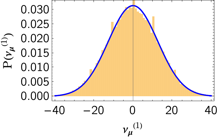
Figure 22: Histogram of the total momentum in the micro-canonical ensemble (144). The curve is a fit to a normal distribution.

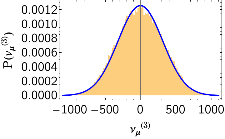
Figure 23: Histogram of the eigenvalues of the third conservation law in the micro-canonical ensemble (144). The curve is a fit to a normal distribution.

The averages for these conserved quantities are as expected zero, but the spread of eigenvalues is very large. Finally we show the probability distribution of the matrix elements of the Bose field $\mathfrak{M}_{\boldsymbol{\lambda},\boldsymbol{\mu}}$ (63) in Fig. 24

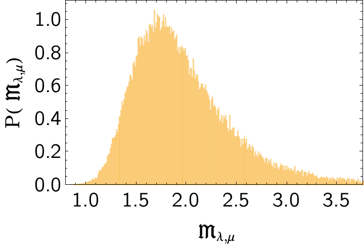
Figure 24: Histogram of the logarithm of matrix elements $\mathfrak{M}_{\boldsymbol{\lambda},\boldsymbol{\mu}}$ (63) between the smooth ket state and bra states obtained by micro-canonical sampling (144).

The micro-canonical sampling described here cannot be used for large particle numbers because it is extremely inefficient. The set of half-odd integer numbers we need to sample has dimension

$$\binom{2I_{\rm max}}{N}\ ,$$ (147)

which grows exponentially with the number of particles. We therefore require more efficient ways of sampling the relevant micro-states.

B.2 Plain vanilla box sampling (PVBS)

The simplest idea for targeting energy eigenstates in the appropriate energy window is to use “box-sampling” of the probability distribution $\varrho(\nu)/D$. The rationale behind this is that for very large numbers of particles almost all these states will correspond to a discretization of $\varrho(\nu)$, cf. the steps leading to our expression for the entropy (16). So what one would do is to approximate $\varrho(\nu)$ as shown in Fig. 25.

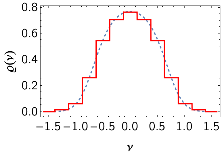
Figure 25: Discretization of the distribution function $\varrho(\nu)$.

To that end we introduce a cut-off $a_{0}$ (which corresponds to $-I_{\rm max}$ in the discussion of the micro-canonical ensemble in the previous subsection). and then sub-divide the $\nu$ axis into intervals $B_{n}=[a_{n-1},a_{n}]$ for $1\leq n\leq M$. The density of $\nu_{j}=I_{j}/L$ in $B_{n}$ is then taken to be

$$\varrho_{n}\equiv D[C(a_{n})-C(a_{n-1})],$$ (148)

where the cumulative PDF $C(\nu)$ is defined in (143). We can straightforwardly translate this into a distribution function of (half-odd) integers that is piecewise constant on the $M$ intervals

$$\bar{B}_{n}=[J_{n-1},J_{n}).$$ (149)

The number of integers in box $\bar{B}_{n}$ is $J_{n}-J_{n-1}$, where in practice we adjust $a_{0}$ in such a way that

$$\sum_{n=1}^{M}N_{n}=N=DL.$$ (150)

We now sample the discretized probability distribution box-by-box: from the (half-odd) integers in $\bar{B}_{n}$ we randomly select $N_{n}$ elements, where

$$N_{n}=\text{Round}\Big{(}L\varrho_{n}\Big{)}.$$ (151)

The total number of different configurations in the resulting sample space is

$$\mathfrak{N}_{M}(\{N_{j}\})=\prod_{n=1}^{M}{{I_{n}-I_{n-1}}\choose{N_{n}}}\equiv e^{L\mathfrak{s}_{M}}\ .$$ (152)

This is much smaller than the number of configurations that needs to be sampled in the micro-canonical ensemble discussed earlier, which corresponds to the choice $M=1$. Importantly, in the double limit

$$\lim_{M\to\infty}\lim_{L\to\infty}\mathfrak{s}_{M}$$ (153)

the number of micro-states produced by this procedure recovers the correct entropy density of the thermal macro-state under consideration. One may therefore expect that this procedure provides a good way of sampling thermal states in finite systems. For a finite number of particles the number of sampled states decreases with $M$ and in our example we find

$$\mathfrak{s}_{3}=1.04\ ,\quad\mathfrak{s}_{5}=1.01\ ,\quad\mathfrak{s}_{7}=0.952773.$$ (154)

These values should be compared with the thermodynamic result $1.20041$. In practice we still need to impose the energy-window restriction (144) so that the actual numbers of states are smaller. For the finite particle numbers of relevance here PVBS does not agree well with the micro-canonical sampling. To show the degree of difference we present results for $M=7$ and our $L=N=32$ example. In Fig. 26 we show the distribution of integers, which reproduces the thermodynamic root distribution function in a satisfactory manner.

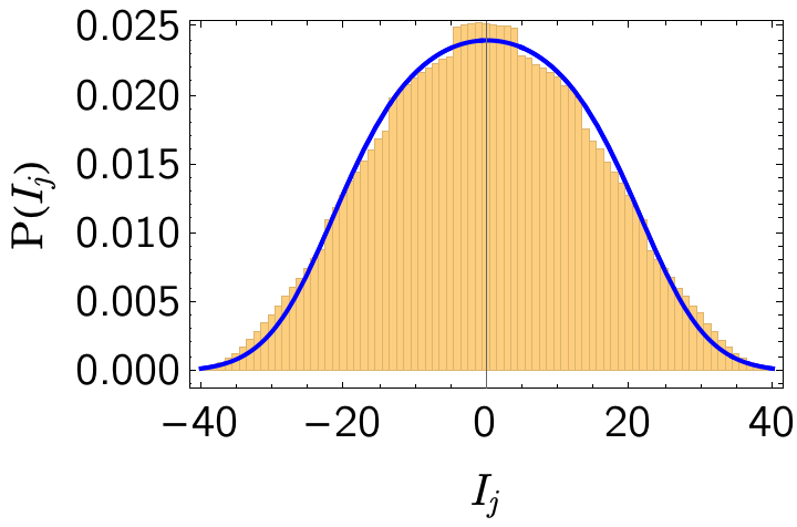
Figure 26: Histogram of integers obtained by PVBS with $M=7$. The blue curve is the thermodynamic root distribution function $\frac{1}{L}\varrho(\frac{I}{L})$.

In Figs 27 and 28 we show the distribution of the total momentum and third conservation laws respectively.

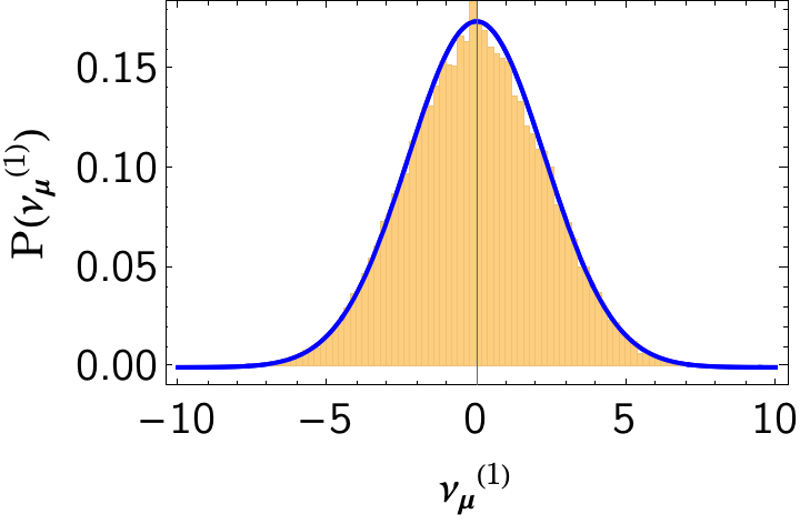
Figure 27: Histogram of the total momentum obtained by PVBS with $M=7$ The curve is a fit to a normal distribution.

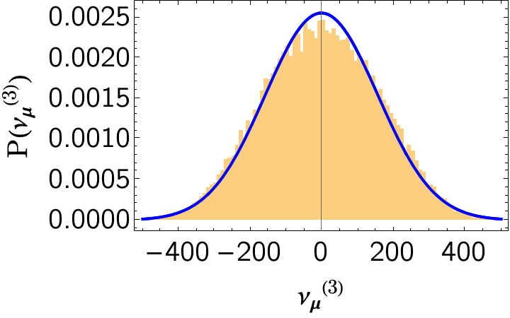
Figure 28: Histogram of the eigenvalues of the third conservation law obtained by PVBS with $M=7$ The curve is a fit to a normal distribution.

We observe that both distributions are very considerably narrower than the corresponding ones for micro-canonical sampling, see Figs 22 and 23. Finally we show the probability distribution of the matrix elements of the Bose field $\mathfrak{M}_{\boldsymbol{\lambda},\boldsymbol{\mu}}$ (63) in Fig. 29.

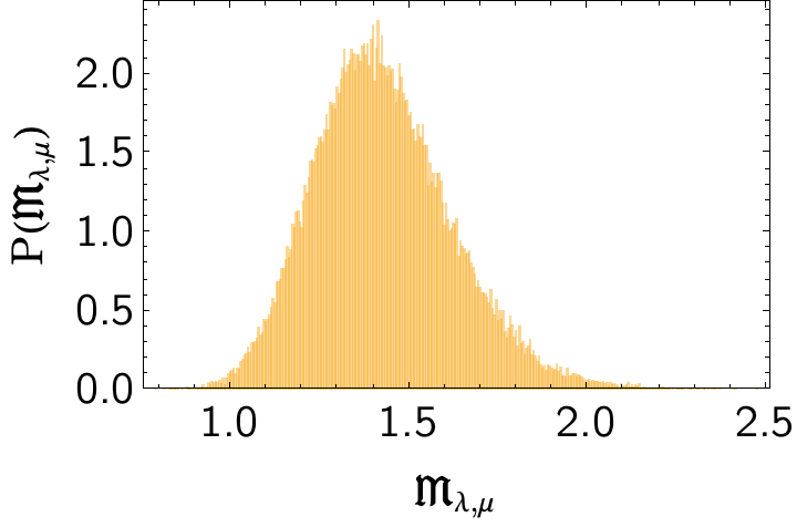
Figure 29: Histogram of the logarithm of matrix elements $\mathfrak{M}_{\boldsymbol{\lambda},\boldsymbol{\mu}}$ (63) between the smooth ket state and bra states obtained by PVBS with $M=7$.

We observe that the typical matrix elements obtained by PVBS are significantly larger than in micro-canonical sampling, cf. Fig. 24. The differences in the probability distributions of matrix elements and the eigenvalues of conserved quantities between PVBS and MC sampling is easy to understand intuitively: by construction PVBS produces significantly smaller fluctuations that the MCE in finite volumes. While the expectation is that these finite-size effects will disappear as the thermodynamic limit is approached, they severely limit the utility of PVBS for the (numerically) accessible system sizes.

B.3 Fluctuating box sampling

As we have seen, in mesoscopic volumes the PVBS accesses a much more restrictive set of energy eigenstates than the MCE. We can make up for this by allowing the box occupation numbers $N_{n}$ to fluctuate. Given a set $B$ of boxes with vacancies ($V_{1},\dots,V_{M}$) we generate a set of occupation numbers $\{N_{j}\}$ such that

$$\sum_{j}N_{j}=N\ ,$$ (155)

where we allow the $N_{j}$ to fluctuate as follows. Let $N^{(\text{PV})}_{j}$ be the PVBS particle numbers. We then take

$$N_{j}=N^{(\text{PV})}_{j}+\delta N_{j}\ ,$$ (156)

where the random integers $\delta N_{j}$ are taken to add up to zero and fulfil

$$\delta N_{j}={\cal O}\big{(}\text{min}\Big{\{}\sqrt{N^{(\text{PV})}_{j}},\sqrt{|V_{j}-N^{(\text{PV})}_{j}|}\Big{\}}\big{)}.$$ (157)

Given a set of particle numbers ($N_{1},\dots,N_{M}$) we calculate the number of micro-states obtained by box-sampling

$$\mathfrak{N}_{M}(\{N_{j}\},\{V_{j}\})=\prod_{n=1}^{M}{{V_{n}}\choose{N_{n}}}\ .$$ (158)

We then generate

$$\bigg{[}\frac{\mathfrak{N}_{M}(\{N_{j}\},\{V_{j}\})}{N_{0}}\bigg{]}$$ (159)

samples from the configuration specified by $\{N_{1},\dots,N_{M}\}$, where $N_{0}$ is some fixed reference number. By construction this procedure increases fluctuations. In practice we may choose the outermost boxes to be larger in order to decrease “tail effects”. Results obtained by this method for $N=L=32$ are shown in Figs 30, 31, 32 and 33.

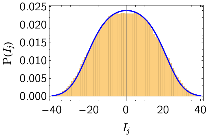
Figure 30: Histograms of integers produced by FBS with $M=7$ and energies in the window $|E-e_{\infty}L|<2$.

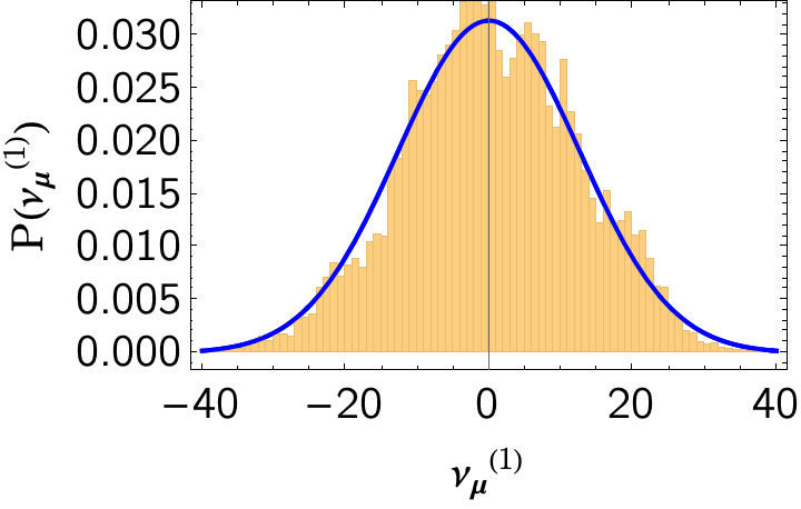
Figure 31: Histograms of momentum produced by FBS with $M=7$ compared to the MCE (solid blue line).

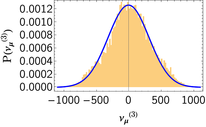
Figure 32: Histograms of $\nu^{(3)}_{\boldsymbol{\lambda}}$ produced by FBS with $M=7$ compared to the MCE (solid blue line).

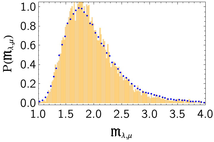
Figure 33: Histogram of the matrix elements between the smooth “ket” state and energy eigenstates in the window $|E-e_{\infty}L|<2$ obtained by FBS (yellow) and in the micro-canonical ensemble (blue dots).

We see that the fluctuating box sampling reproduces the results of the MCE fairly well. However, this requires the fluctuations are taken to be sufficiently strong. In particular, if we make them weaker by changing the coefficient that multiplies the r.h.s. in the expression for $\delta N_{j}$ the agreement becomes worse. This is as expected. FBS is significantly slower than PVBS and becomes computationally very expensive for large particle numbers.

B.4 Random sampling (RS)

The distribution of integers in the micro-canonical ensemble is well-described by the thermodynamic distribution function $\varrho(\nu)/D$. This suggests that a random sampling of this probability distribution should reproduce the MCE. The difficulty is that we must generate non-repeating integers. Our starting point is the set of integers

$$S_{M}=\{j|-I_{\rm max}\leq j\leq I_{\rm max}\}\ ,\quad M=2I_{\rm max}+1.$$ (160)

and an associated discrete probability distribution

$$P_{M}=\{p_{1},\dots,p_{M}\}\ .$$ (161)

In practice we take $P_{M}$ to be a discretization of self-consistently determined continuous PDF $P(\nu)$. The corresponding set of cumulative probabilities is

$${\cal C}_{M}=\{C_{n}=\sum_{j=1}^{n-1}p_{j}\ ,\quad n=1,\dots,2I_{\rm max}+2\}.$$ (162)

We now generate a (real) random number $r$ in the interval $[0,1]$ and determine the integer $j$ such that

$$C_{j-1}<r<C_{j}\ .$$ (163)

We then remove the integer $j$ from the set $S_{M}$ and define a new discrete probability distribution

$$P_{M-1}=\Big{\{}\frac{p_{1}}{1-p_{j}},\dots,\frac{p_{j-1}}{1-p_{j}},\frac{p_{j+1}}{1-p_{j}},\dots,\frac{p_{M}}{1-p_{j}}\Big{\}}\$$ (164)

and the associated cumulative probability distribution ${\cal C}_{M-1}$. Repeating this procedure $N$ times results in a set of distinct integers $\{I_{1},\dots,I_{N}\}$. Finally, we impose that the probability distribution of these sets of integers is a discretization of the (normalized) root density $\varrho(\nu)/D$. Importantly, this requires an initial probability distribution $P(\nu)$ that is different from $\varrho(\nu/D)$. The PDF required to produce the normalized root distribution upon random sampling is shown in the main text in Fig. 2.

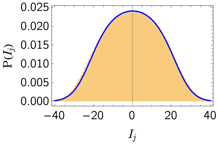
Figure 34: Histogram of integers by RS using the probability distribution $P(\nu)$ shown in Fig. 2. The solid curve is the root distribution function $\varrho(\nu)/D$.

In Figs 35, 36 and 37 we show the histograms obtained by our random sampling procedure for the eigenvalues of momentum, the third conservation law and the matrix elements of the Bose field operator between the smooth “ket” state and energy eigenstates in the window $|E-e_{\infty}L|<2$.

Figure 35: Histograms of the total momentum obtained by random sampling under the constraint that $|E-e_{\infty}L|<2$ for $N=L=32$. The results in the micro-canonical ensemble are shown as the solid blue line.

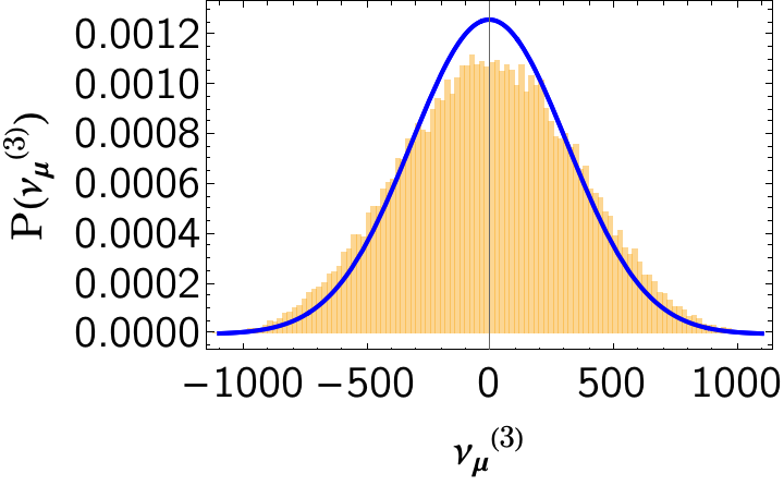
Figure 36: Histograms of the third conservation law obtained by random sampling under the constraint that $|E-e_{\infty}L|<2$ for $N=L=32$. The results in the micro-canonical ensemble are shown as the solid blue line.

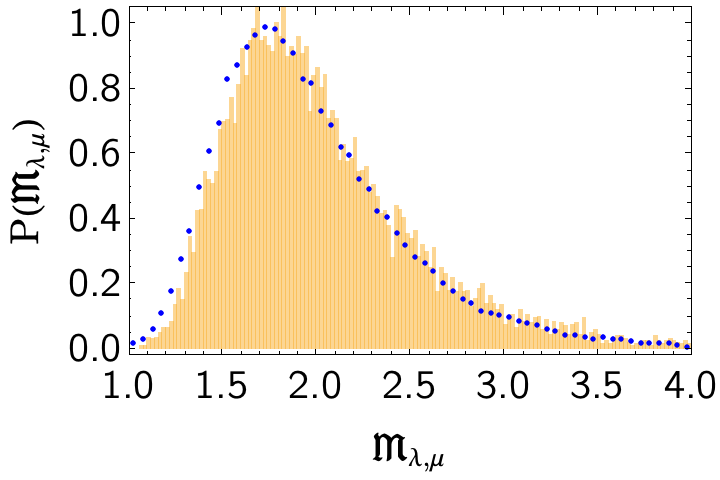
Figure 37: Histograms of the matrix elements of the Bose field operator between the smooth “ket” state and energy eigenstates in the window $|E-e_{\infty}L|<2$ for $N=L=32$ obtained by random sampling (yellow) and in the micro-canonical ensemble (blue dots).

We observe that the results are in good agreement with those obtained by micro-canonical sampling. We conjecture that the remaining differences, in particular in $P(\nu^{(3)}_{\boldsymbol{\mu}}$, are at least partially caused by the cutoff in the MC sampling procedure.

B.5 Simplified random sampling (SRS)

The random sampling algorithm described above is somewhat slow. We therefore use the simplified algorithm described in section III.1 of the main text. The latter is faster as it treats the constraint that all (half-odd) integers must be distinct in a much simpler fashion. It nevertheless gives results that agree with RS within the statistical error in all cases we have tested. Examples are shown in Figs 38, 39 and 40. Here we have chosen a larger energy window $|E-e_{\infty}L|<10$.

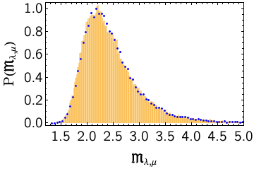
Figure 38: Histogram the matrix elements of the Bose field operator between the smooth “ket” state and energy eigenstates in the window $|E-e_{\infty}L|<10$ obtained by SRS (yellow) and analogous result for RS (blue dots).

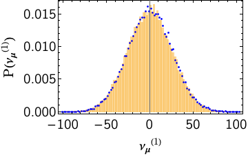
Figure 39: Histogram of the eigenvalues of momentum for energy eigenstates in the window $|E-e_{\infty}L|<10$ obtained by SRS (yellow) and analogous result for RS (blue dots).

Figure 40: Histogram of the eigenvalues of the third conservation law for energy eigenstates in the window $|E-e_{\infty}L|<10$ obtained by SRS (yellow) and analogous result for RS (blue dots).

B.6 Interacting case

As all sampling methods discussed above are based on drawing sets of non-repeating (half-odd) integers $\{I_{j}\}$ from a probability distribution they generalize in a straightforward way to the interacting case. The main differences are:

• The target PDF $P(I_{j})$ is obtained from (38) by solving the nonlinear integral equations (37) (for thermal macro-states).

• For $0<c<\infty$ we need to (numerically) solve the Bethe equations once we have generated a set $\{I_{j}\}$.

References

- Deutsch [1991] J. M. Deutsch, Quantum statistical mechanics in a closed system, Physical review a 43, 2046 (1991).
- Srednicki [1994] M. Srednicki, Chaos and quantum thermalization, Physical review e 50, 888 (1994).
- Srednicki [1999] M. Srednicki, The approach to thermal equilibrium in quantized chaotic systems, Journal of Physics A: Mathematical and General 32, 1163 (1999).
- D’Alessio et al. [2016] L. D’Alessio, Y. Kafri, A. Polkovnikov, and M. Rigol, From quantum chaos and eigenstate thermalization to statistical mechanics and thermodynamics, Advances in Physics 65, 239 (2016).
- Rigol et al. [2008] M. Rigol, V. Dunjko, and M. Olshanii, Thermalization and its mechanism for generic isolated quantum systems, Nature 452, 854 (2008).
- Rigol and Santos [2010] M. Rigol and L. F. Santos, Quantum chaos and thermalization in gapped systems, Phys. Rev. A 82, 011604 (2010).
- Steinigeweg et al. [2013] R. Steinigeweg, J. Herbrych, and P. Prelovšek, Eigenstate thermalization within isolated spin-chain systems, Physical Review E 87, 012118 (2013).
- Kim et al. [2014] H. Kim, T. N. Ikeda, and D. A. Huse, Testing whether all eigenstates obey the eigenstate thermalization hypothesis, Physical Review E 90, 052105 (2014).
- Beugeling et al. [2014] W. Beugeling, R. Moessner, and M. Haque, Finite-size scaling of eigenstate thermalization, Physical Review E 89, 10.1103/physreve.89.042112 (2014).
- Beugeling et al. [2015] W. Beugeling, R. Moessner, and M. Haque, Off-diagonal matrix elements of local operators in many-body quantum systems, Physical Review E 91, 10.1103/physreve.91.012144 (2015).
- Chandran et al. [2016] A. Chandran, M. D. Schulz, and F. J. Burnell, The eigenstate thermalization hypothesis in constrained hilbert spaces: A case study in non-abelian anyon chains, Phys. Rev. B 94, 235122 (2016).
- Mondaini and Rigol [2017] R. Mondaini and M. Rigol, Eigenstate thermalization in the two-dimensional transverse field ising model. ii. off-diagonal matrix elements of observables, Phys. Rev. E 96, 012157 (2017).
- Nation and Porras [2018] C. Nation and D. Porras, Off-diagonal observable elements from random matrix theory: distributions, fluctuations, and eigenstate thermalization, New Journal of Physics 20, 103003 (2018).
- Yoshizawa et al. [2018] T. Yoshizawa, E. Iyoda, and T. Sagawa, Numerical large deviation analysis of the eigenstate thermalization hypothesis, Physical Review Letters 120, 10.1103/physrevlett.120.200604 (2018).
- Khaymovich et al. [2019] I. M. Khaymovich, M. Haque, and P. A. McClarty, Eigenstate thermalization, random matrix theory, and behemoths, Physical Review Letters 122, 10.1103/physrevlett.122.070601 (2019).
- Pappalardi et al. [2022] S. Pappalardi, L. Foini, and J. Kurchan, Eigenstate thermalization hypothesis and free probability, Phys. Rev. Lett. 129, 170603 (2022).
- Biroli et al. [2010] G. Biroli, C. Kollath, and A. M. Läuchli, Effect of rare fluctuations on the thermalization of isolated quantum systems, Physical Review Letters 105, 10.1103/physrevlett.105.250401 (2010).
- Ikeda et al. [2013] T. N. Ikeda, Y. Watanabe, and M. Ueda, Finite-size scaling analysis of the eigenstate thermalization hypothesis in a one-dimensional interacting bose gas, Physical Review E 87, 10.1103/physreve.87.012125 (2013).
- Alba [2015] V. Alba, Eigenstate thermalization hypothesis and integrability in quantum spin chains, Physical Review B 91, 10.1103/physrevb.91.155123 (2015).
- Khatami et al. [2013] E. Khatami, G. Pupillo, M. Srednicki, and M. Rigol, Fluctuation-dissipation theorem in an isolated system of quantum dipolar bosons after a quench, Physical Review Letters 111, 10.1103/physrevlett.111.050403 (2013).
- LeBlond et al. [2019] T. LeBlond, K. Mallayya, L. Vidmar, and M. Rigol, Entanglement and matrix elements of observables in interacting integrable systems, Physical Review E 100, 10.1103/physreve.100.062134 (2019).
- Brenes et al. [2020] M. Brenes, J. Goold, and M. Rigol, Low-frequency behavior of off-diagonal matrix elements in the integrable XXZ chain and in a locally perturbed quantum-chaotic XXZ chain, Physical Review B 102, 10.1103/physrevb.102.075127 (2020).
- LeBlond and Rigol [2020] T. LeBlond and M. Rigol, Eigenstate thermalization for observables that break hamiltonian symmetries and its counterpart in interacting integrable systems, Physical Review E 102, 10.1103/physreve.102.062113 (2020).
- Mierzejewski and Vidmar [2020] M. Mierzejewski and L. Vidmar, Quantitative impact of integrals of motion on the eigenstate thermalization hypothesis, Physical Review Letters 124, 10.1103/physrevlett.124.040603 (2020).
- Zhang et al. [2022] Y. Zhang, L. Vidmar, and M. Rigol, Statistical properties of the off-diagonal matrix elements of observables in eigenstates of integrable systems, Physical Review E 106, 10.1103/physreve.106.014132 (2022).
- Korepin et al. [1993] V. Korepin, N. Bogoliubov, and A. Izergin, Quantum Inverse Scattering Method and Correlation Functions, Cambridge Monographs on Mathematical Physics (Cambridge University Press, 1993).
- Takahashi [1999] M. Takahashi, Thermodynamics of One-Dimensional Solvable Models (Cambridge University Press, 1999).
- Essler et al. [2005] F. H. L. Essler, H. Frahm, F. Göhmann, A. Klümper, and V. E. Korepin, The one-dimensional Hubbard model (Cambridge University Press, 2005).
- Gaudin [2014] M. Gaudin, The Bethe Wavefunction (Cambridge University Press, 2014).
- Smirnov [1992] F. A. Smirnov, Form factors in completely integrable models of quantum field theory, Vol. 14 (World Scientific, 1992).
- Korepin [1982] V. E. Korepin, Calculation of norms of bethe wave functions, Communications in Mathematical Physics 86, 391 (1982).
- Slavnov [1989] N. A. Slavnov, Calculation of scalar products of wave functions and form factors in the framework of the algebraic bethe ansatz, Teoreticheskaya i Matematicheskaya Fizika 79, 232 (1989).
- Caux et al. [2007] J.-S. Caux, P. Calabrese, and N. A. Slavnov, One-particle dynamical correlations in the one-dimensional bose gas, Journal of Statistical Mechanics: Theory and Experiment 2007, P01008 (2007).
- Piroli and Calabrese [2015] L. Piroli and P. Calabrese, Exact formulas for the form factors of local operators in the lieb–liniger model, Journal of Physics A: Mathematical and Theoretical 48, 454002 (2015).
- Lieb and Liniger [1963] E. H. Lieb and W. Liniger, Exact analysis of an interacting Bose gas. I. The general solution and the ground state, Phys. Rev. 130, 1605 (1963).
- Bethe [1931] H. Bethe, Zur theorie der metalle: I. eigenwerte und eigenfunktionen der linearen atomkette, Zeitschrift für Physik 71, 205 (1931).
- Bloch et al. [2008] I. Bloch, J. Dalibard, and W. Zwerger, Many-body physics with ultracold gases, Rev. Mod. Phys. 80, 885 (2008).
- Cazalilla et al. [2011] M. A. Cazalilla, R. Citro, T. Giamarchi, E. Orignac, and M. Rigol, One dimensional bosons: From condensed matter systems to ultracold gases, Rev. Mod. Phys. 83, 1405 (2011).
- Kitanine et al. [2012] N. Kitanine, K. Kozlowski, J. M. Maillet, N. Slavnov, and V. Terras, Form factor approach to dynamical correlation functions in critical models, Journal of Statistical Mechanics: Theory and Experiment 2012, P09001 (2012).
- Fabbri et al. [2015] N. Fabbri, M. Panfil, D. Clément, L. Fallani, M. Inguscio, C. Fort, and J.-S. Caux, Dynamical structure factor of one-dimensional bose gases: Experimental signatures of beyond-luttinger-liquid physics, Physical Review A 91, 043617 (2015).
- Meinert et al. [2015] F. Meinert, M. Panfil, M. J. Mark, K. Lauber, J.-S. Caux, and H.-C. Nägerl, Probing the excitations of a lieb-liniger gas from weak to strong coupling, Physical review letters 115, 085301 (2015).
- Kozlowski [2015] K. K. Kozlowski, Large-distance and long-time asymptotic behavior of the reduced density matrix in the non-linear schrödinger model, in Annales Henri Poincaré, Vol. 16 (Springer, 2015) pp. 437–534.
- Doyon and Spohn [2017] B. Doyon and H. Spohn, Drude weight for the lieb-liniger bose gas, SciPost Physics 3, 039 (2017).
- Doyon [2018] B. Doyon, Exact large-scale correlations in integrable systems out of equilibrium, SciPost Phys. 5, 54 (2018).
- Granet and Essler [2020] E. Granet and F. H. L. Essler, A systematic -expansion of form factor sums for dynamical correlations in the Lieb-Liniger model, SciPost Phys. 9, 82 (2020).
- Granet [2021] E. Granet, Low-density limit of dynamical correlations in the lieb–liniger model, Journal of Physics A: Mathematical and Theoretical 54, 154001 (2021).
- Caux and Essler [2013] J.-S. Caux and F. H. L. Essler, Time evolution of local observables after quenching to an integrable model, Phys. Rev. Lett. 110, 257203 (2013).
- Kormos et al. [2013] M. Kormos, A. Shashi, Y.-Z. Chou, J.-S. Caux, and A. Imambekov, Interaction quenches in the one-dimensional bose gas, Phys. Rev. B 88, 205131 (2013).
- De Nardis et al. [2014] J. De Nardis, B. Wouters, M. Brockmann, and J.-S. Caux, Solution for an interaction quench in the lieb-liniger bose gas, Phys. Rev. A 89, 033601 (2014).
- Kormos et al. [2014] M. Kormos, M. Collura, and P. Calabrese, Analytic results for a quantum quench from free to hard-core one-dimensional bosons, Phys. Rev. A 89, 013609 (2014).
- De Nardis and Panfil [2015] J. De Nardis and M. Panfil, Density form factors of the 1d bose gas for finite entropy states, Journal of Statistical Mechanics: Theory and Experiment 2015, P02019 (2015).
- Piroli et al. [2016] L. Piroli, P. Calabrese, and F. H. L. Essler, Multiparticle bound-state formation following a quantum quench to the one-dimensional bose gas with attractive interactions, Phys. Rev. Lett. 116, 070408 (2016).
- Bouchoule and Dubail [2022] I. Bouchoule and J. Dubail, Generalized hydrodynamics in the one-dimensional bose gas: theory and experiments, J. Stat. Mech. 2022, 014003 (2022).
- Robinson et al. [2021] N. Robinson, A. de Klerk, and J.-S. Caux, On computing non-equilibrium dynamics following a quench, SciPost Physics 11, 10.21468/scipostphys.11.6.104 (2021).
- Granet and Essler [2021] E. Granet and F. H. L. Essler, Systematic strong coupling expansion for out-of-equilibrium dynamics in the Lieb-Liniger model, SciPost Phys. 11, 68 (2021).
- Essler [2019] F. H. L. Essler, Chapter contents, Integrability: From Statistical Systems to Gauge Theory: Lecture Notes of the Les Houches Summer School: Volume 106, June 2016 106, 319 (2019).
- Essler [2022] F. H. L. Essler, A short introduction to generalized hydrodynamics, Physica A: Statistical Mechanics and its Applications , 127572 (2022).
- Creamer et al. [1980] D. B. Creamer, H. Thacker, and D. Wilkinson, Quantum Gel’fand-Levitan method as a generalized Jordan-Wigner transformation, Phys. Lett. B 92, 144 (1980).
- Girardeau [1960] M. Girardeau, Relationship between systems of impenetrable bosons and fermions in one dimension, Journal of Mathematical Physics 1, 516 (1960).
- Veness et al. [2017] T. Veness, F. H. L. Essler, and M. P. A. Fisher, Quantum disentangled liquid in the half-filled Hubbard model, Phys. Rev. B 96, 195153 (2017).
- De Nardis and Panfil [2018] J. De Nardis and M. Panfil, Edge singularities and quasilong-range order in nonequilibrium steady states, Phys. Rev. Lett. 120, 217206 (2018).
- Davies and Korepin [2011] B. Davies and V. E. Korepin, Higher conservation laws for the quantum non-linear Schrödinger equation, arXiv preprint arXiv:1109.6604 (2011).
- Lukyanov [1995] S. Lukyanov, Free field representation for massive integrable models, Communications in Mathematical Physics 167, 183 (1995).
- Essler and Fagotti [2016] F. H. L. Essler and M. Fagotti, Quench dynamics and relaxation in isolated integrable quantum spin chains, Journal of Statistical Mechanics: Theory and Experiment 2016, 064002 (2016).
- Granet et al. [2020] E. Granet, M. Fagotti, and F. H. L. Essler, Finite temperature and quench dynamics in the transverse field ising model from form factor expansions, SciPost Physics 9, 033 (2020).
- Calabrese et al. [2012] P. Calabrese, F. H. L. Essler, and M. Fagotti, Quantum quench in the transverse field ising chain: I. time evolution of order parameter correlators, Journal of Statistical Mechanics: Theory and Experiment 2012, P07016 (2012).
- Bertini et al. [2014] B. Bertini, D. Schuricht, and F. H. L. Essler, Quantum quench in the sine-Gordon model, J. Stat. Mech. 2014, P10035 (2014).
- Schuricht and Essler [2012] D. Schuricht and F. H. L. Essler, Dynamics in the ising field theory after a quantum quench, Journal of Statistical Mechanics: Theory and Experiment 2012, P04017 (2012).
- Note [1] We note however that essentially equally good descriptions of the data are obtained by two-parameter fits to .
- [70] F. H. L. Essler, Work in progress. .
- Bulchandani et al. [2022] V. B. Bulchandani, D. A. Huse, and S. Gopalakrishnan, Onset of many-body quantum chaos due to breaking integrability, Phys. Rev. B 105, 214308 (2022).